A Tutorial on Adaptive Design Optimization

Jay I. Myunga#, Daniel R. Cavagnarob, and Mark A. Pitta

aDepartment of Psychology, Ohio State University, Columbus, OH 43210bMihaylo College of Business and Economics, California State University, Fullerton, CA 92831

{myung.1@osu.edu, dcavagnaro@exchange.fullerton.edu, pitt.2@osu.edu}#Corresponding author

May 16, 2013

Abstract

Experimentation is ubiquitous in the field of psychology and fundamental to the advancementof its science, and one of the biggest challenges for researchers is designing experiments thatcan conclusively discriminate the theoretical hypotheses or models under investigation. Therecognition of this challenge has led to the development of sophisticated statistical methods thataid in the design of experiments and that are within the reach of everyday experimental scientists.This tutorial paper introduces the reader to an implementable experimentation methodology,dubbed Adaptive Design Optimization, that can help scientists to conduct “smart” experimentsthat are maximally informative and highly efficient, which in turn should accelerate scientificdiscovery in psychology and beyond.

1 Introduction

Imagine an experiment in which each and every stimulus was custom tailored to be maximallyinformative about the question of interest, so that there were no wasted trials, participants, orredundant data points. Further, what if the choice of design variables in the experiment (e.g.,stimulus properties and combinations, testing schedule, etc.) could evolve in real-time as data werecollected, to take advantage of information about the response the moment it is acquired (andpossibly alter the course of the experiment) rather than waiting until the experiment is over andthen deciding to conduct a follow-up?

The ability to fine-tune an experiment on the fly makes it possible to identify and capitalizeon individual differences as the experiment progresses, presenting each participant with stimuli thatmatch a particular response pattern or ability level. More concretely, in a decision making experi-ment, each participant can be given choice options tailored to her or his response preferences, ratherthan giving every participant the same, pre-selected list of choice options. As another example, inan fMRI experiment investigating the neural basis of decision making, one could instantly analyzeand evaluate each image that was collected and adjust the next stimulus accordingly, potentiallyreducing the number of scans while maximizing the usefulness of each scan.

1

The implementation of such idealized experiments sits in stark contrast to the current prac-tice in much of psychology of using a single design, chosen at the outset, throughout the course ofthe experiment. Typically, stimulus creation and selection are guided by heuristic norms. Strate-gies to improve the informativeness of an experiment, such as creating all possible combinationsof levels of the independent variables (e.g., three levels of task difficulty combined with five levelsof stimulus duration), actually work against efficiency because it is rare for all combinations to beequally informative. Making matters worse, equal numbers of participants are usually allotted toeach combination of treatments for statistical convenience, even the treatments that may not beinformative. Noisy data are often combatted in a brute-force way by simply collecting more ofthem (this is the essence of a power analysis). The continued use of these practices is not the mostefficient use of time, money, and participants to collect quality data.

A better, more efficient way to run an experiment would be to dynamically alter the designin response to observed data. The optimization of experimental designs has a long history instatistics dating back to the 1950s (e.g., Lindley, 1956; Box and Hill, 1967; Atkinson and Federov,1975; Atkinson and Donev, 1992; Berry, 2006). Psychometricians have been doing this for decadesin computerized adaptive testing (e.g., Weiss and Kingsbury, 1984), and psychophysicists havedeveloped their own adaptive tools (e.g., Cobo-Lewis, 1997; Kontsevich and Tyler, 1999). The majorhurdle in applying adaptive methodologies more broadly has been computational: Quantitativetools for identifying the optimal experimental design when testing formal models of cognition havenot been available. However, recent advances in statistical computing (Doucet et al., 2001; Robertand Casella, 2004) have laid the groundwork for a paradigmatic shift in the science of data collection.The resulting new methodology, dubbed adaptive design optimization (ADO, Cavagnaro et al.,2010), has the potential to more broadly benefit experimentation in cognitive science and beyond.

In this tutorial, we introduce the reader to adaptive design optimization. The tutorial isintended to serve as a practical guide to apply the technique to simple cognitive models. As such,it assumes a rudimentary level of familiarity with cognitive modeling, such as how to implementquantitative models in a programming or graphical language, how to use maximum likelihood esti-mation to determine parameter values, and how to apply model selection methods to discriminatemodels. Readers with little familiarity with these techniques might find Section 3 difficult to fol-low, but should otherwise be able to understand most of the other sections. We begin by reviewingapproaches to improve inference in cognitive modeling. Next we describe the technical details ofadaptive design optimization, covering the computational and implementation details. Finally, wepresent an example application of the methodology for designing experiments to discriminate sim-ple models of memory retention. Readers interested in more technical treatments of the materialshould consult (Myung and Pitt, 2009; Cavagnaro et al., 2010).

2 Why Optimize Designs?

2.1 Not All Experimental Designs Are Created Equal

To illustrate the importance of optimizing experimental designs, suppose that a researcher is in-terested in empirically discriminating between formal models of memory retention. The topic ofretention has been studied for over a century. Years of research have shown that a person’s abilityto remember information just learned drops quickly for a short time after learning and then levelsoff as more and more time elapses. The simplicity of this data pattern has led to the introduction

2

of numerous models to describe the change over time in the rate at which information is retained inmemory. Through years of experimentation with humans (and animals), a handful of the modelshave proven to be superior to the rest of the field (Wixted and Ebbesen, 1991), although morerecent research suggests that they are not complete (Oberauer and Lewandowsky, 2008). Thesemodels describe the probability p of correctly recalling a stimulus item as a function of the time tsince study. Two particular models that have received considerable attention are the power model,p = a(t + 1)−b, and the exponential model, p = ae−bt. Both models predict that memory recalldecays gradually as the lag time between study and test phases increases.

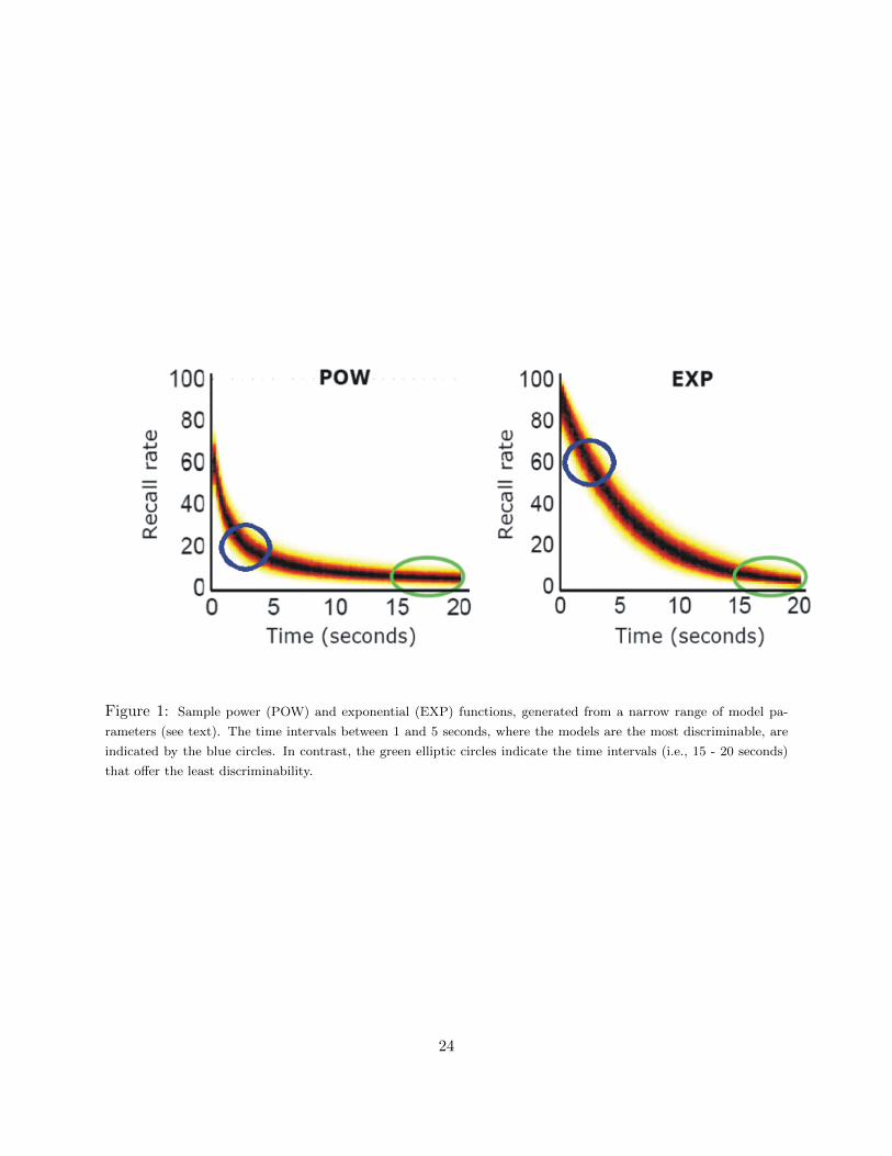
Figure 1 shows predictions of power and exponential models obtained under restrictedranges of parameter values (i.e., 0.65 < a < 0.85 and 0.75 < b < 0.95 for the power model, and0.80 < a < 1.00 and 0.10 < b < 0.20 for exponential model). Suppose that the researcher conductsan experiment to compare these model predictions by probing memory at different lag times, whichrepresent values of a design variable in this experiment. Visual inspection of the figure suggests thatlag times between 15 and 20 seconds would be bad designs to use because in this region predictionsfrom both models are virtually indistinguishable from each other. In contrast, times between 1and 5 seconds, where the models are separated the most, would make good designs for the modeldiscrimination experiment.

In practice, however, the problem of identifying good designs is a lot more complicated thanthe idealized example in Figure 1. It is more often the case that the researchers have little infor-mation about the specific ranges or values of model parameters under which experimental data arelikely to be observed. Further, the models under investigation may have many parameters so visualinspection of their predictions across designs would be simply impossible. This is where quanti-tative tools for optimizing designs can help identify designs that make experiments more efficientand more effective than what is possible with current practices in experimental psychology. In theremainder of this tutorial, we will describe how the optimization of designs can be accomplished.For an illustrative application of the methodology for discriminating the aforementioned models ofretention, the reader may skip ahead to Section 4.

2.2 Optimal Design

In psychological inquiry, the goal of the researcher is often to distinguish between competing expla-nations of data (i.e., theory testing) or to estimate characteristics of the population along certainpsychological dimensions, such as the prevalence and severity of depression. In cognitive modeling,these goals become ones of model discrimination and parameter estimation, respectively. In bothendeavors, the aim is to make the strongest inference possible given the data in hand. The scien-tific process is depicted inside in the rectangle in Figure 2a: first, the values of design variablesare chosen in an experiment, then the experiment is carried out and data are collected, and finally,data modeling methods (e.g., maximum likelihood estimation, Bayesian estimation) are applied toevaluate model performance at the end of this process.

Over the last several decades, significant theoretical and computational advances have beenmade that have greatly improved the accuracy of inference in model discrimination (e.g., Burnhamand Anderson, 2010). Model selection methods in current use include the Akaike InformationCriterion (Akaike, 1973), the Bayes factor (Jeffreys, 1961; Kass and Raftery, 1995), and MinimumDescription Length (Rissanen, 1978; Grunwald, 2005), to name a few. In each of these methods, amodel’s fit to the data is evaluated in relation to its overall flexibility in fitting any data pattern, toarrive at a decision regarding which model of two competing models to choose (Pitt et al., 2002).

3

As depicted in in Figure 2a, data modeling is applied to the back end of the experiment after datacollection is completed. Consequently, the methods themselves are limited by the quality of theempirical data collected. Inconclusive data will always be inconclusive, making the task of modelselection difficult no matter what data modeling method is used. A similar problem presents itselfin estimating model parameters from observed data, regardless of whether maximum likelihoodestimation or Bayesian estimation is used.

Because data modeling methods are not foolproof, attention has begun to focus on thefront end of the data collection enterprise, before an experiment is conducted, developing methodsthat optimize the experimental design itself. Design optimization (DO, Myung and Pitt, 2009)is a statistical technique, analogous to model selection methods, that selectively chooses designvariables (e.g., treatment levels and values, presentation schedule) with the aim of identifyingan experimental design that will produce the most informative and useful experimental outcome(Atkinson and Donev, 1992). Because experiments can be difficult to design, the consequences ofdesign choices and the quality of the proposed experiment are not always predictable, even if one isan experienced researcher. DO can remove some of the uncertainty of the design process by takingadvantage of the fact that both the models and some of the design variables can be quantifiedmathematically.

How does DO work? To identify an optimal design, one must first define the design space,which consists of the set of all possible values of design variables that are directly controlled by theexperimenter. The researcher must define this set by considering the properties of the variablesbeing manipulated. For example, a variable on an interval scale may be discretized. The coarserthe discretization, the fewer the number of designs. Given five design variables, each with ten levels,there are 100,000 possible designs.

In addition, the model being evaluated must be expressed in formal, mathematical terms,whether it is a model of visual processing, recognition memory, or decision making. A mathematicalframework provided by Bayesian decision theory (Chaloner and Verdinelli, 1995) offers a principledapproach to design optimization. Specifically, each potential design is viewed as a gamble whosepayoff is determined by the outcome of an experiment conducted with that design. The payoffrepresents some measure of the goodness or the utility of the design. Given that there are manypossible outcomes that an experiment could produce, one estimates the expected utility (i.e., pre-dicted utility) of a given design by computing the average payoffs across all possible outcomes thatcould be observed in an experiment carried out with the chosen design. The design with the high-est expected utility is then identified as the optimal design. To conceptualize the problem slightlydifferently, if one imagines a distribution representing the utility of all designs, ordered from worstto best, the goal of DO is to identify the design at the extreme (best) endpoint of the distribution.

2.3 An Adaptive Approach to Experimentation: Adaptive Design Optimization

DO is a one-shot process. An optimal design is identified, applied in an experiment, and thendata modeling methods are used to aid in interpreting the results, as depicted in Figure 2a,. Thisinference process can be improved by using what is learned about model performance in the datamodeling stage to optimize the design still further. Essentially, these two stages are connected asshown in Figure 2b, yielding adaptive design optimization (ADO).

ADO is an integrative approach to experimentation that leverages, on-line, the complemen-tary strengths of design optimization and data modeling. The result is an efficient and informativemethod of scientific inference. In ADO, the optimal experimental design is updated at intervals

4

during the experiment, which we refer to as stages. It can be as frequent as after every trial orafter a number of trials (e.g., a mini experiment). Factors such as the experimental methodologybeing used will influence the frequency of updating. As depicted in Figure 2b, updating involvesrepeating data modeling and design optimization. More specifically, within a Bayesian framework,adaptive design optimization is cast as a decision problem where, at the end of each stage, the mostinformative design for the next stage (i.e., the design with the highest expected utility) is soughtbased on the design and outcomes of the previous stage. This new stage is then carried out withthat design, and the resulting data are analyzed and modeled. This is followed by identifying a newdesign to be used in the next stage.1 This iterative process continues until an appropriate stoppingcriterion is reached.

Various additional (pragmatic) decisions arise with ADO. In particular, one must decidehow many mini experiments will be carried out, either in succession within a single testing session(e.g., one hour). A critical factor, which is likely only determined with piloting, is how many stagesare necessary to obtain decisive model discrimination or stable parameter estimation. It may bethat testing would be required across days, but to date we have not found this to be necessary.

By using all available information about the models and how the participant has responded,ADO collects data intelligently. It has three attractive properties that make it particularly wellsuited for evaluating computational models. These pertain to the informativeness of the datacollected in the experiment, the sensitivity of the method to individual differences, and the efficiencyof data collection. We briefly elaborate on each.

As noted above, design optimization and data modeling are synergistic techniques thatare united in ADO to provide a clear answer to the question of interest. Each mini-experimentis designed, or each trial chosen, such that the evidence pertaining to the question of interest,whether it be estimating a participant’s ability level or discriminating between models, accumulatesas rapidly as possible. This is accomplished by using what is learned from each stage to narrow inon those regions of the design space that will be maximally informative in some well-defined sense.

The adaptive nature of the methodology, by construction, controls for individual differencesand thus makes it well suited for studying the most common and often largest source of variancein experiments. When participants are tested individually using ADO, the algorithm adjusts (i.e.,optimizes) the design of the experiment to the performance of that participant, thereby maximizingthe informativeness of the data at an individual participant level. Response strategies and groupdifferences can be readily identified. This capability also makes ADO ideal for studies in which fewparticipants can be tested (e.g., rare memory or language disorders).

Another benefit of using an intelligent data collection scheme is that it speeds up the exper-iment, possibly resulting in a substantial savings of time, fewer trials and participants, and lowercost. This savings can be significant when using expensive technology (e.g., fMRI) or numerous sup-port staff (e.g., developmental or clinical research). Similarly, in experiments using hard-to-recruitpopulations (children, elderly, mental patients), application of ADO means fewer participants, allwithout sacrificing the quality of the data or the quality of the statistical inference.

The versatility and efficiency of ADO has begun to attract attention in various disciplines.It has been used recently for designing neurophysiology experiments (Lewi et al., 2009), adaptiveestimation of contrast sensitivity functions of human vision (Kujala and Lukka, 2006; Lesmes et al.,

1Adaptive design optimization is conceptually and theoretically related to active learning in machine learning(Cohn et al., 1994, 1996) and also to policy iteration in dynamic programming (Sutton and Barto, 1998; Powell,2007).

5

2006, 2010; Vul and Bergsma, 2010), designing systems biology experiments (Kreutz and Timmer,2009), detecting exoplanets in astronomy (Loredo, 2004), conducting sequential clinical trials (e.g.,Wathen and Thall, 2008), and adaptive selection of stimulus features in human information acqui-sition experiments (Nelson, 2005; Nelson et al., 2011). Perhaps the most well-known example ofADO, albeit a very different implementation of it, is computerized adaptive testing in psychology(e.g., Hambleton et al., 1991; van der Linden and Glas, 2000). Here, an adaptive sequence of testitems, which can be viewed in essence as experimental designs, is chosen from an item bank takinginto account an examinee’s performance on earlier items so as to accurately infer the examinee’sability level with the fewest possible items.

In our lab, we have used ADO to adaptively infer a learner’s representational state incognitive development experiments (Tang et al., 2010), to discriminate models of memory retention(Cavagnaro et al., 2010, 2011), and to optimize risky decision making experiments (Cavagnaroet al., 2013a,b). These studies have clearly demonstrated the superior efficiency of ADO to thealternative non-ADO methods, such as random and fixed designs (e.g., Cavagnaro et al., 2010,2013a, Fig. 3 & Fig. 7, respectively).

3 The Nuts and Bolts of Adaptive Design Optimization

In this section we describe the theoretical and computational aspects of ADO in greater detail. Thesection is intended for readers who are interested in applying the technique to their own cognitivemodeling. Our goal is to provide readers with the basic essentials of implementing ADO in theirown experiments. Figure 3 show a schematic diagram of the ADO framework that involves a seriesof steps. In what follows we discuss each step in turn.

3.1 Preliminaries

Application of ADO requires that each model under consideration be formulated as a statisticalmodel defined as a parametric family of probability distributions, p(y|θ, d)’s, each of which specifiesthe probability of observing an experimental outcome (y) given a parameter value (θ) and a designvalue (d). That is, the data vector y is a sample drawn from the probability distribution (oftencalled the sampling distribution) for given values of the parameter vector θ and of the design vectord.

To be concrete, consider the exponential model of memory retention, defined by p = ae−bt,that describes the probability of correct recall of a stimulus item (e.g., word or picture) as a functionof retention interval t and parameter vector θ = (a, b) where 0 < a < 1 and b > 0. In a typicalexperiment, there is a study phase in which participants learn a list of words. After a retentioninterval, which can range from fractions of a second to minutes, participants are tested on theirmemory for the list of words. Data are scored as the number of correctly recalled items (y) out ofa fixed number of independent Bernoulli trials (n), all given at a single retention interval t. Notethat the retention interval is the design variable whose value is being experimentally manipulated,i.e., d = t.

Under the assumption that the exponential model describes retention performance, theexperimental outcome would follow the binomial probability distribution of the form

p(y|θ = (a, b), t) =n!

(n− y)! y!

(ae−bt

)y (1− ae−bt

)n−y, (1)

6

where y = 0, 1, ..., n. When retention performance is probed over multiple time points of the designvariable, d = (t1, ..., tq), the data are summarized into a discrete vector y = (y1, ..., yq) with eachyi ∈ {0, ..., n}, and the overall probability distribution of the outcome vector y is then given by

p(y|θ = (a, b), d) =

q∏i=1

n!

(n− yi)! yi!

(ae−bti

)yi (1− ae−bti

)n−yi. (2)

ADO is formulated in a Bayesian statistical framework. It is beyond the scope of this tutorialto review this vast literature, and instead, the reader is directed to consult Bayesian textbooks(e.g., Robert, 2001; Gelman et al., 2004; Gill, 2007; Kruschke, 2010). The Bayesian formulation ofADO requires specification of priors for model parameters, denoted by p(θ). There are a plethoraof methods proposed in the Bayesian literature for choosing appropriate priors, whether they aresubjective, objective, or empirical priors (Carlin and Louis, 2000, for a review). Practically speaking,however, what is important to note is that ADO results might strongly depend upon the particularform of the prior employed so it must be chosen with careful thought and proper justification.

As a concrete example, for the above two parameters, a and b, of the exponential modelof retention, one might choose to employ the following prior defined by the product of a Betaprobability density for parameter a and an exponential probability density for parameter b

p(θ = (a, b)) =Γ(α+ β)

Γ(α)Γ(β)aα−1(1− a)β−1 λe−λb, (3)

for α = 4, β = 2, and λ = 10, for instance. Combining the prior distribution in the above equationwith the probability distribution of the outcome vector in Eq. (2) by Bayes rule yields the posteriordistribution as

p(θ = (a, b)|y, d) =p(y|θ = (a, b), d) p(θ = (a, b))∫ ∫p(y|θ = (a, b), d) p(θ = (a, b)) dadb

. (4)

Having specified a model’s probability distribution and the prior and posterior distributionsof model parameters, we now discuss the details of the ADO framework

3.2 Design Optimization

As mentioned earlier, ADO is a sequential process consisting of a series of optimization-experimentationstages. An optimal design is sought on the basis of the present state of knowledge, which is coded inthe prior. Next, data are collected with the optimal design. The observed outcomes are then usedto update the prior to the posterior, which in turn becomes the prior on the next iteration of theADO process. As such, the design is optimized in each ADO stage, and this design optimization(DO) step involves solving an optimization problem defined as

d∗ = argmaxd

U(d), (5)

for some real-valued function U(d) that is a metric of goodness or utility of design d.Formally and without loss of generality, we define the utility function U(d) to be optimized

7

as

U(d) =∑m

p(m)

∫ ∫u(d, θm, ym) p(ym|θm, d) p(θm) dym dθm, (6)

where m = {1, 2, ...,K} is one of a set of K models being considered, and ym is the outcomevector resulting from a hypothetical imaginary experiment, in lieu of a real one, conducted withdesign d under model m, and θm is a parameter vector of model m (e.g., Chaloner and Verdinelli,1995; Myung and Pitt, 2009; Nelson et al., 2011). In the above equation, p(m) denotes the priormodel probability of model m. The “local” utility function, u(d, θm, ym), measures the utility ofan imaginary experiment carried out with design d when the data generating model is m, theparameters of the model take the value θm, and the outcome ym is produced.

On the left side of the above equation is what is sometimes referred to as the global utilityfunction U(d) (so as to distinguish it from the local utility function defined above), and is defined asthe expectation of u(·) averaged over the models, parameters, and observations, taken with respectto the model prior p(m), the parameter prior p(θm), and the probability distribution p(ym|θm, d),respectively.

To evaluate the global utility U(d) in Eq. (6), one must provide explicit specifications forthree functions: (1) the model and parameter priors, p(m) and p(θm); (2) the probability distribu-tion given parameter θm and design d, p(ym|θm, d); and (3) the local utility function u(d, θm, ym).These are shown on the left side of Figure 3, which is a schematic illustration of ADO. The firsttwo functions were discussed in the preceding section. We discuss the specification of the third, thelocal utility function, next.

3.3 Local Utility Function

From Eq. (5), it can be seen that the global utility being optimized is nothing but an average valueof the local utility over all possible data samples and model parameters, weighted by the likelihoodfunction and the model and parameter priors. As such, selection of a local utility function in ADOdetermines the characteristics of what constitutes an optimal design. One should therefore choosea local utility function that is appropriate for the specific goal of the experiment.

Generally speaking, the cognitive modeler conducts an experiment with one of two goals inmind: parameter estimation or model discrimination. In parameter estimation, given a model ofinterest, the goal is to estimate the values of the model’s parameters as accurately as possible withthe fewest experimental observations. On the other hand, in model discrimination, given a set ofmultiple candidate models, the goal is to identify the one that is closest in some defined sense tothe underlying data generating model, again using the fewest number of observations. Below wediscuss possible forms of the local utility function one can use for either goal.

A simple and easy-to-understand local utility function for parameter estimation is of thefollowing form:

u(d, θ = (θ1, ..., θk), y) =

k∑i=1

E(θi)

SD(θi), (7)

where k is the number of parameters, and E(θi) and SD(θi) stand for the mean and standarddeviation, respectively, of the posterior distribution of parameter θi, denoted as p(θi|y, d). Notethat by construction, K in Eq. (6) is equal to 1 in parameter estimation so the subscript m isskipped in Eq. (7). The above local utility function is defined as a sum of “inverse” standard

8

deviations of parameters weighted by their means so that the function value does not depend uponthe unit in which each parameter is measured. Note that a larger value of u(d, θ, y) is translated intoless parameter variability overall, which in turn implies a more accurate estimate of the parameters.One may also consider other variations of the above form, each suitably chosen taking into accountthe particular purpose of the experiment at hand.

Sometimes, the choice of a local utility function can be driven by the principled choiceof a global utility function. Perhaps the most commonly employed global utility function in theliterature is the following, motivated from information theory:

U(d) = I(Θ;Y |d) (8)

which is the mutual information between the parameter random variable Θ and the outcome randomvariable Y conditional upon design d, i.e., Y |d. The mutual information is defined in terms of twoentropic measures as I(Θ;Y |d) = H(Θ) −H(Θ|Y, d) (Cover and Thomas, 1991). In this equationH(Θ) = −

∫p(θ) log p(θ) dθ is the Shannon entropy (i.e., uncertainty) of the parameter random

variable Θ and H(Θ|Y, d) = −∫p(θ|y, d) log p(θ|y, d) dθ is the conditional entropy of Θ given the

outcome random variable Y and design d (Note that the expression log throughout this tutorialdenotes the natural logarithm of base e.). As such, U(d) in Eq. (8) measures the reduction inuncertainty about the values of the parameters that would be provided by the observation of anexperimental outcome under design d. In other words, the optimal design is the one that extractsthe maximum information about the model’s parameters.

The information theoretic global utility function in Eq. (8) follows from setting the localutility function as

u(d, θ, y) = logp(θ|y, d)

p(θ), (9)

which is the log ratio of posterior to prior probabilities of parameters. Thus, the local utilityfunction is set up to favor the design that results in the largest possible increase in certainty aboutthe model’s parameters upon an observed outcome of the experimental event.

Turning the discussion from parameter estimation to model discrimination, we can alsodevise a corresponding pair of information theoretic utility functions for the purpose of modeldiscrimination. That is, the following global and local utility functions have an information theoreticinterpretation (Cavagnaro et al., 2010, p. 895)

U(d) = I(M ;Y |d), (10)

u(d, θm, ym) = logp(m|y, d)

p(m),

where I(M ;Y |d) is the mutual information between the model random variable M and the outcomerandom variable conditional upon design d, Y |d. In the above equation, p(m|y, d) is the posteriormodel probability of model m obtained by Bayes rule as p(m|y, d) = p(y|m, d)p(m)/p(y|d), wherep(y|m, d) =

∫p(y|θm, d)p(θm) dθm and p(y|d) =

∑m p(y|m, d)p(m). Note the similarity between

these two mutual information measures and those in Eq. (8) and Eq. (8); the parameter randomvariable Θ is replaced by the model random variable M . This switch makes sense when the goal ofexperimentation is to discriminate among a set of models, not among possible parameter values ofa single model.

The mutual information I(M ;Y |d) is defined as H(M)−H(M |Y, d), where H(M) is the en-

9

tropy of the model random variable M , quantifying the uncertainty about the true, data-generatingmodel, and H(M |Y, d) is the conditional entropy of M given Y and d. As such, the global utilityfunction U(d) in Eq. (10) is interpreted as the amount of information about the true, data-generating model that would be gained upon the observation of an experimental outcome underdesign d; thus, the optimal design is the one that extracts the maximum information about thedata-generating model. The corresponding local utility function u(d, θm, ym) in the same equationis given by the log ratio of posterior to prior model probabilities. Accordingly, the design withthe largest possible increase in certainty about model m upon the observation of an experimentaloutcome with design d is valued the most. Finally, it is worth noting that by applying Bayes rule,one can express the log ratio in an equivalent form as log p(m|y,d)

p(m) = log p(y|m,d)p(y|d) .

3.4 Bayesian Updating of the Optimal Design

The preceding discussion presents a framework for identifying a single optimal design. It is straight-forward to extend it to the sequential process of ADO. This is done by updating the model andparameter priors, as depicted in Figure 3. To extend it formally, let us introduce the subscriptsymbol s = {1, 2, ...} to denote an ADO stage, which could be a single trial or a sequence of tri-als comprising a mini-experiment, depending on how finely the experimenter wishes to tune thedesign. Suppose that at stage s the optimal design d∗s was obtained by maximizing U(d) in Eq.(6) on the basis of a set of model and parameter priors, ps(m) and ps(θm) with m = {1, 2, ...,K},respectively. Suppose further that a mini-experiment with human participants was subsequentlycarried out with design d∗s, and an outcome vector zs was observed. The observed data are used toupdate the model and parameter priors to the posteriors by Bayes rule (e.g., Gelman et al., 2004;Cavagnaro et al., 2010) as

ps+1(m) =p1(m)∑K

k=1 p1(k)BF(k,m)(zs|d∗s), (11)

ps+1(θm) =p(zs|θm, d∗s) ps(θm)∫p(zs|θm, d∗s) ps(θm) dθm

,

where m = {1, 2, ...,K}. In this equation, BF(k,m)(zs|d∗s) denotes the Bayes factor defined as theratio of the marginal likelihood of model k to that of model m, specifically,

BF(k,m)(zs|d∗s) =

∫p(zs|θk, d∗s) ps(θk) dθk∫p(zs|θm, d∗s) ps(θm) dθm

(12)

The resulting posteriors in Eq. (11) are then used as the “priors” to find an optimal design d∗s+1

at the next stage of ADO, again using the same equation in (6) but with s = s+ 1.To summarize, each ADO stage involves the execution of the design optimization, exper-

iment, and Bayesian updating steps in that order, as illustrated in Figure 3. This adaptive andsequential ADO procedure continues until an appropriate stopping criterion is met. For example,the process may stop whenever one of the parameter posteriors is deemed to be “sufficiently peaked”around the mean in parameter estimation, or in model discrimination, whenever posteriors exceeda pre-set threshold value (e.g., p(m) > 0.95).

10

3.5 Computational Methods

To find the optimal design d∗ in Eq. (5) on each stage of ADO entails searching for a solution inhigh dimensional design space. Since the equation cannot be solved analytically, the search processinvolves alternating between proposing a candidate solution and evaluating the objective functionfor the given solution. The optimization problem is further exacerbated by the fact that the globalutility function, which is defined in terms of a multiple integral over the data and parameter spaces,has in general no easy-to-evaluate, closed-form expression, requiring the integral to be evaluatednumerically. This is a highly nontrivial undertaking, computationally speaking. We discuss twonumerical methods for solving the design optimization problem.

3.5.1 Grid Search

Grid search is an intuitive, heuristic optimization method in which the design space is disretizedinto a finite number of mutually disjoint partitions of equal volumes. The global utility function isevaluated for each partition one at a time, exhaustively, and the partition with the largest globalutility value is chosen as the optimal design.

The global utility is estimated numerically using a Monte Carlo procedure. To show how,suppose that we wish to evaluate the utility function at design dg. Given a particular design dg,this is done by first drawing a large number of Monte Carlo triplet samples, (k, θk, yk)’s, fromthe model prior, parameter prior, and sampling distribution, respectively, and then estimating theglobal utility in Eq. (6) as a sample average of the local utility as

U(dg) ≈1

N

N∑i=1

u(dg, θk(i)(i), yk(i)(i)

), (13)

for large N (e.g., N = 104). In the above equation, k(i) (= {1, 2, ...,K}) is the ith model indexsampled from the model prior p(m), θk(i)(i) is the ith sample drawn randomly from the param-eter prior p(θk(i)) of model k(i), yk(i)(i) is the i-th data sample from the probability distributionp(yk(i)|θk(i)(i), dg) of model k(i) given parameter θk(i)(i) and design dg.

This way, the approximate numerical estimate in Eq. (13) is evaluated for each de-sign in the discretized design space. To be concrete, consider a five-dimensional design vectord = (d1, d2, ..., d5), where each di is a point in the [0, 1] interval. The design space can bediscretized into a finite grid consisting of ten equally spaced values for each dimension (e.g.,d1 = {0.05, 0.15, ..., 0.95}. This yields 105 design points on which the computation in Eq. (13)must be performed. An algorithmic sketch of the grid search algorithm is shown in Figure 4.

It is important to note that integral forms of the local utility function, such as the formin Eq. (10), cannot be evaluated directly in general. In such cases, each value of the local utilityfunction u

(dg, θk(i)(i), yk(i)(i)

)in Eq. (13) must itself be estimated by another Monte Carlo method,

thereby introducing an additional computational cost.To summarize, grid search, though simple and intuitive, is an expensive optimization algo-

rithm to apply, especially for higher dimensional problems. This is because as the dimensionalityof the design increases, the number of discretized points necessary to evaluate grows exponentially,which is a problem in statistics known the curse of dimensionality (Bellman, 2003).

11

3.5.2 Sequential Monte Carlo Search

The grid search based optimization algorithm discussed in the preceding section requires an exhaus-tive and systematic search of the design space for an optimal design, and thus becomes increasinglycomputationally intractable as the dimension of the space grows large. For large design spaces, it ispreferable to use an “intelligent” optimization algorithm that mitigates the curse of dimensionalityby exploring the space selectively and efficiently, focusing the search on the most promising regionsthat are likely to contain the optimal solution. In this section we introduce one such method knownas sequential Monte Carlo (SMC) search.

SMC, or particle filtering (Doucet et al., 2001), is a Monte Carlo method for simulating ahigh-dimensional probability distribution of arbitrary shape. SMC is a sequential analogue of theMakov chain Monte Carlo (MCMC) algorithm in statistics (Robert and Casella, 2004) and consistsof multiple MCMC chains, called particles, that are run in parallel with information exchangetaking place among the particles periodically. Further, the interactions between the individualparticles evolve over time in a nature-inspired, genetic algorithmic process.

SMC can be adapted to solve the design optimization problem in Eqs. (5 - 6), as shownin Muller et al. (2004) and Amzal et al. (2006). The basic idea of SMC-based design optimizationis to regard the design variable d as a random variable, treat U(d) as a probability distribution,and then recast the problem of finding the optimal design as a simulation-based sampling problemwith U(d) as the target probability distribution. The optimal design is then obtained as the designvalue (d∗) that corresponds to the highest peak of the target probability distribution.

Figure 5 illustrates the SMC-based search method for design optimization. To show howthe method works, let us pretend that the solid curve in the top graph of the figure representsthe probability distribution U(d) plotted against the span of designs d. The plot shows that theoptimal design d∗ corresponding to the highest peak of U(d) is located at about 150. Now, supposethat we draw random samples from the distribution. This is where SMC is necessary. It allowsus to generate random samples from virtually any distribution without having to determine itsnormalizing constant. Shown also in the top panel is a histogram of 2000 such random samples.Note that the histogram closely approximates the target distribution, as it should.

We have not yet solved the design optimization problem. Note that with SMC, we onlycollect random samples of the design variable, but without their corresponding utility values. Con-sequently, the challenge is to identify, from the collected SMC samples, the one with the highestutility as the optimal design. One simple way to solve this challenge is to have all or most ofthe random samples clustered around the optimal design point. This is done by “sharpening” thedistribution U(d) using simulated annealing (Kirkpatrick et al., 1983). That is, instead of samplingfrom the distribution U(d), we would sample from an augmented distribution U(d)J for some pos-itive integer J > 1. The solid curve in the middle panel of Figure 5 is one such distribution, withJ = 5. Notice how much more peaked it is than the original distribution U(d). Shown under thecurve is a histogram of 2000 random samples drawn from U(d)5, again using SMC. As the logicgoes, if we keep raising the value of J , which is often called the inverse annealing temperature (i.e.,J = 1/T ) in the literature, then for some large J , the corresponding augmented distribution U(d)J

would have just one, most-prominent peak. This is indeed what is shown in the bottom panel of thefigure for J = 35. Note that the only peak of the distribution is above the optimal point d∗ = 150,and further, that virtually all of the 2,000 samples drawn from the augmented distribution are nowclustered around the optimal design. Once we get to this point, we can then estimate the optimaldesign point as a simple average of the sampled design values, for example.

12

In practice, it could be prohibitively difficult to sample directly from U(d) or its augmenteddistributions U(d)J in the algorithm described above. This is because the application of SMCnecessarily requires the ability to routinely and quickly calculate the value of U(d) for any value ofthe design variable d. The global utility function, however, takes the form of a multiple integral,which is generally not amenable to direct calculation.

To address this challenge, Muller has proposed an ingenious computational idea that makesit possible to draw random samples from U(d) in Eq. (6) using SMC, but without having to evaluatethe multiple integral directly (Muller, 1999). The key idea is to define an auxiliary probabilitydistribution h(·) of the form

h(d, {m}, {ym}, {θm}) = α

[K∑m=1

p(m)u(d, θm, ym)

][K∏m=1

p(ym|θm, d) p(θm)

](14)

where α (> 0) is the normalizing constant of the auxiliary distribution. Note that for the trick towork, the local utility function u(d, θm, ym) must be non-negative for all values of d, θm, and ym sothat h(·) becomes a legitimate probability distribution. It is then straightforward to show that byconstruction, the global utility function U(d) is nothing but (up to a proportionality constant) themarginal distribution h(d) that is obtained by marginalizing h(d, {m}, {ym}, {θm}) with respect toall of its variables, except for the design variable d (see Cavagnaro et al., 2010, p. 892), in otherwords, U(d) = 1

αh(d).Having defined the auxiliary distribution h(·) in Eq. (14), let us return to the SMC

based optimization method. This revised method works much the same way except for one sig-nificant modification: instead of simulating U(d), we simulate the whole auxiliary distributionh(d, {m}, {ym}, {θm}). This means that using SMC along with simulated annealing, we first collecta large number (e.g., 105) of random draws {d, {m}, {ym}, {θm}}’s from the auxiliary distribution,and then, from the sample, we empirically estimate the desired distribution U(d) by keeping onlyd’s but discarding all the rest (i.e., {m}’s, {ym}’s, {θm}’s). This way, instead of directly simulatingthe target distribution U(d), which is generally not possible, we achieve the same goal indirectlyby way of the auxiliary distribution h(d, ·), which is much easier to simulate. The SMC searchalgorithm is shown in Figure 6.2

Before closing this section, we briefly discuss a few technical aspects of implementing theSMC based design optimization algorithm.

First, regarding the inverse annealing temperature J , generally speaking, the inverse tem-perature (J) should be raised rather slowly over a series of SMC iteration steps (e.g., Bolte andThonemann, 1996). For example, one may employ an annealing schedule function of the formρ(t) = a log(b ∗ t + c) (a, b, c > 0), where t denotes the SMC iteration number, and a, b and c arethe scaling parameters to be tuned for the given design optimization problem.

Second, in SMC search, the decision as to when to stop the search process must be made.This can often be achieved through visual inspection of the current SMC sample of designs. If almostall of the sampled designs are highly clustered around one another, this may be an indication thatthe SMC search process has converged to a solution. Formally, one can base the decision on somequantitative criterion. For example, one may define a “peakedness” measure, δ(S), that assessesthe extent to which a sample of random draws d’s, denoted by S, is judged to be drawn from a

2The C++ source code that implements the SMC search algorithm is available for download from the webhttp://faculty.psy.ohio-state.edu/myung/personal/do.html.

13

highly peaked and unimodal probability distribution, appropriately defined. By construction, onemay define δ(S) to be non-negative and real-valued such that the higher its value, the more peakedthe underlying distribution.

For further implementation details of SMC, the interested reader is directed to Andrieuet al. (2003), an excellent tutorial on SMC in particular and MCMC in general. The reader mayalso find it useful to consult Myung and Pitt (2009, Appendix A), which provides greater detailabout the iterative steps of SMC-based design optimization.

3.6 Implementation of ADO-based Experiments

While ADO takes much of the guesswork out of designing an experiment, implementation of anADO-based experiment still requires several decisions to be made. One such decision is the lengthof each mini-experiment. At one extreme, each mini-experiment could consist of just one trial. Inthis case, model and parameter estimates would be updated after each trial, and the DO step aftereach trial would consist in finding the design for the next trial. At the other extreme, the entireexperiment could be one mini-experiment. In this case, a set of jointly optimal stimuli would befound prior to collecting any data, and Bayesian updating would only be done after all data werecollected.

There are several, practical tradeoffs involved in deciding on the length of each mini-experiment. One on hand, more frequent Bayesian updating means that information gained fromeach observation is utilized more quickly and more efficiently. From that standpoint, it would bebest to make each mini-experiment as short as possible. On the other hand, since each DO steponly looks forward as far as the next mini experiment, the shorter each mini-experiment is, themore myopic the DO step is. For example, if the next mini-experiment consists of just trial thenthe DO step considers designs for the next trial independently of any other future trials that mayoccur. In contrast, when the next mini-experiment includes several trials, the DO step considersthe designs for those trials simultaneously, and finds designs that are jointly optimal for the nextmini-experiment. One should also consider that this joint optimization problem is more computa-tionally demanding, and hence slower, than the single-design optimization problem. This tradeoffis illustrated more concretely in the next section, with two examples of ADO-based experiments.

Another important decision to make before implementing ADO is which prior distributionsto use. The ideal approach would be to use informative priors that accurately reflect individualperformance. Such priors could potentially be derived from pilot testing, general consensus inthe field, or the results of other experiments in the literature. The prior drives the selection ofstimuli in the initial stages of the experiment, but since the parameter distributions are updatedsequentially, the data will quickly trump all but the most pathological prior distributions. There-fore, using informative priors is helpful but not essential to implementing ADO. In the absence ofreliable information from which to construct an informative prior, a vague, noninformative priorthat does not give appreciably different densities to those regions of the parameter space wherethere is a reasonable fit may be used instead. In this regard, the reader is directed to Kass andWasserman (1996) which provides an excellent review of the state of the art on the construction ofnoninformative priors.

One way to assess the adequacy of the prior assumptions is through simulation experiments.In a simulation experiment with ADO, optimal designs are derived from the global utility functionbased parameter estimates as usual, but rather than collecting data from human subjects at thosedesigns, the data are simulated from one of the models under consideration. More precisely, the

14

simulation starts with equal model probabilities and some form of prior parameter estimates (eitherinformative or uninformative), and an optimal design is sought for the first mini-experiment. Afterdata are generated, model probabilities and parameter estimates are updated, and the process isrepeated. The idea of the simulation is to verify that ADO can correctly identify the data-generatingmodel in a reasonable amount of time (in terms of both the number of trials, and computation time).Separate simulations should be run with each model under consideration as the data-generatingmodel to verify that the true, data-generating model can always be uncovered. Biases in the priorsmay then be assessed by examining the posterior model probabilities. For example, if the posteriorprobability of that model rises rather sharply in the initial stages of the experiment even whenit is not the true data-generating model, this might be an indication that the priors are biasedtoward a particular model. If the bias is strong enough then it may be impossible to overcome in areasonable number of trials. Besides helping to diagnose biases in the priors, such simulations arealso helpful for planning how many trials are likely to be necessary to achieve the desired level ofdiscrimination among the models under consideration.

One other practical consideration in implementing an ADO-based experiment is how toprogram it. Since the ADO algorithm is computationally intensive, speed is paramount. Therefore,it is recommended to use an efficient, low-level programming language such as C++. Our labgroup found a 10-fold speed increase upon translating the code from Matlab to C++.3 However,the entire experiment does not need to be programmed in the same language. We have found iteffective to program the graphical user interface (GUI) in a higher level language such as PERLor Matlab, and have the GUI call on a C++ executable to do the computational heavy lifting ofthe DO step and the Bayesian updating. One advantage of this split is that it is easily adaptedto different hardware architectures. For example, the GUI can be run simultaneously on severalclient machines, each of which send their data to a dedicated server, which then sends the optimaldesigns back to the clients.

4 Illustrative Example

To further illustrate how ADO works, we will demonstrate its implementation in a simulationexperiment intended to discriminate between power and exponential models of retention. Theeffectiveness of ADO for discriminating between these models has been demonstrated in simulation(Cavagnaro et al., 2010) and in experiments with human participants (Cavagnaro et al., 2009, 2011).The intention of this demonstration is provide an easy to understand companion to the technicaland theoretical details of the previous section.

The power and exponential functions of retention, as given earlier, are p = a(t + 1)−b andp = ae−bt respectively, where p is the probability of correct recall given the time t between study andtest and a and b are non-negative parameters. The power and exponential models of retention aredefined by equipping these decay functions with the binomial likelihood function that was definedin Eq. (2).4 Many experiments have been performed to discriminate between these models, butthe results have been ambiguous at best (see Rubin and Wenzel, 1996, for a thorough review).

3Since the conversion, many of Matlab’s base functions have been vectorized, so the speed-up may be less dramaticnow.

4Although more sophisticated models have been shown to give fuller accounts of retention (e.g., Oberauer andLewandowsky, 2008), the simplicity of the power and exponential functions along with the difficulty of discriminatingbetween them provides an ideal setting in which to illustrate ADO.

15

Models of retention aim to describe retention rates across a continuous time interval (e.g.,between zero and forty seconds), but due to practical limitations, experimenters can only testretention at a select handful of specific times. In a typical experiment, data are collected througha sequence of trials, each of which assesses the retention rate at a single time point, called the lagtime. The lag time, as a design variable in the experiment, is the length of time between the studyphase, in which a participant is given a list of words to memorize, and the test phase, in whichretention is assessed by testing how many words the participant can correctly recall from the studylist. In the retention literature, the number of lag times and their spacing have varied betweenexperiments. Some have used as few as 3, others as many as 15. Some have used uniform spacing(e.g., d = {1,2,3,4,5}), but most use something close to geometry spacing (e.g., d = {1,2,4,8,16}).The use of a geometric spread of retention intervals is an informed choice that has evolved throughmany years of first-hand experience and trial-and-error.

Since the lag times are numerical and they fit directly into the likelihood functions of themodels under investigation, they are an ideal candidate to be optimized by ADO. Unlike what hasbeen done in the majority of studies in the literature, an experiment using ADO does not rely ona predetermined spacing of the lag times. Rather, the lag times are derived on-the-fly, for eachparticipant individually, based on each participant’s performance at the preceding lag times.

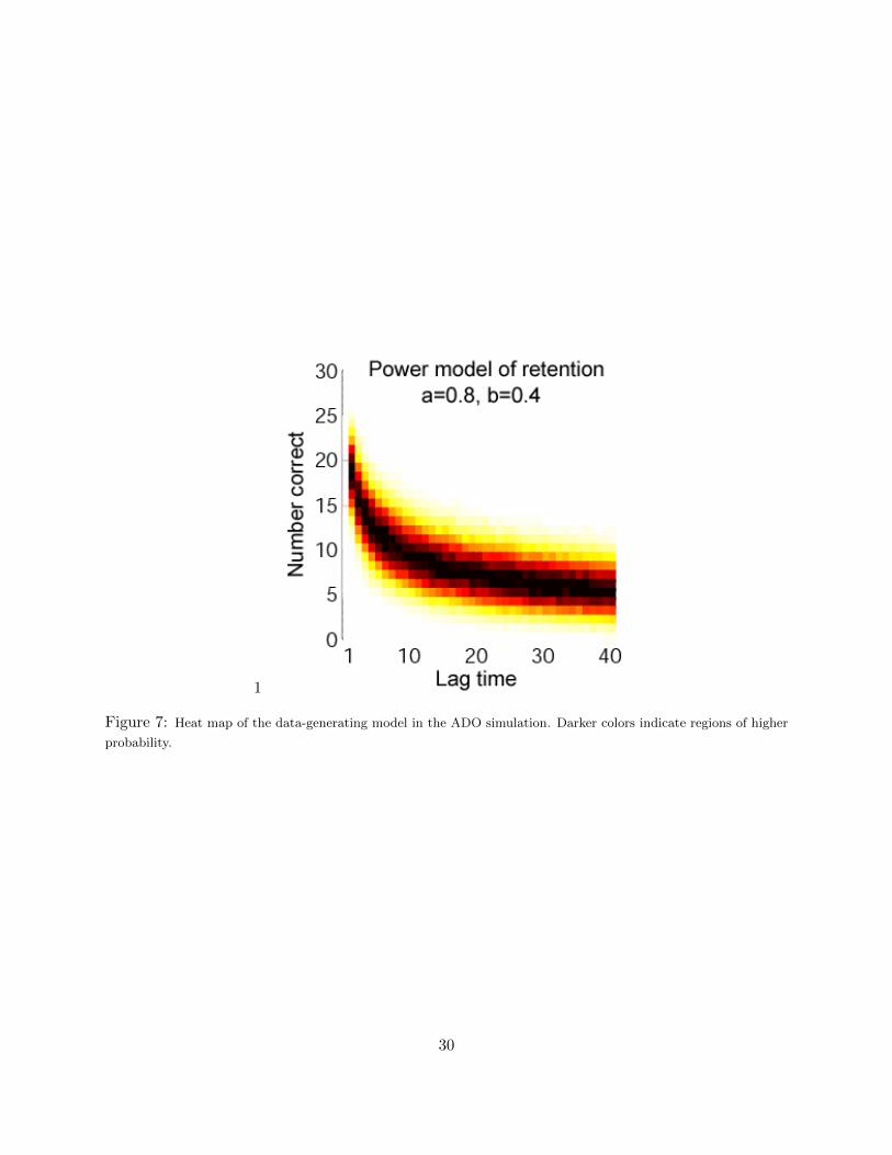
To illustrate, we will walk through a simulation experiment in which ADO is used to selectlag times for discriminating between power and exponential models of retention. The simulation willconsist of ten adaptive stages, each consisting of 30 trials, where each trial represents an attempt torecall one study item after a specified lag time. The lag will be selected by ADO, and will be fixedacross trials within the same stage. To match the practical constraints of an actual experiment,only integer-valued lag times between 1 and 40 seconds will be considered. Recall of study itemsat the lag times selected by ADO will be simulated by the computer. Specifically, the computerwill generate the number of correctly recalled study items by simulating 30 Bernoulli trials withprobability of success p = 0.80(t + 1)−0.40. In other words, the data-generating model will be thepower model with a = 0.80 and b = 0.40.

The data-generating model is depicted in Figure 7. Since the model is probabilistic, evenwith fixed parameters, it is depicted with a heat map in which darker colors indicate regions ofhigher probability. For example, the heat map shows that at a lag time of 40 seconds, the model ismost likely to generate 6 or 7 correct responses out of 30 trials, and the model is extremely unlikelyto generate less than 3 or more than 10 correct responses.

Foreknowledge of the data-generating model will not be programmed into the ADO part ofthe simulation. Rather, ADO must learn the data-generating model by testing at various lag times.Thus, ADO will be initialized with uninformative priors that will be updated after each stage basedon the data collected in that stage. If the data clearly discriminate between the two models thenthe posterior probability of the power model should rise toward 1.0 as data are collected, indicatingincreasing confidence that the data-generating process is a power model. On the other hand, if thedata do not clearly discriminate between the two models then the model probabilities should bothremain near 0.5, indicating continued uncertainty about which model is generating the data.

The initial predictions of ADO about the data-generating process can be seen in Figure8. The figure shows heat maps for both the power model (left) and exponential model (right), ascoded in the following priors: a ∼ Beta(2,1), b ∼ Beta(1,4) for the former, and a ∼ Beta(2,1),b ∼ Beta(1,80) for the latter. Since ADO does not know which model is generating the data, itassigns an initial probability of 0.5 to each one. In addition, since ADO begins with uninformative

16

priors on parameters, the heat maps show that almost any retention rate is possible at any lagtime. As data are collected in the experiment, the parameter estimates should become tighter andthe corresponding heat maps should start to look as much like that of the data-generating modelas the functional form will allow.

With the framework of the experiment fully laid out, we are ready to begin the simulation.To start, ADO searches for an optimal lag time for first stage. Since there are only 40 possible lagtimes to consider (the integers 1 to 40), the optimal one can be found by directly evaluating Eq.(10) at each possible lag time.5 Doing so reveals that the lag time with the highest expected utilityis t = 7, so it is adopted as the design for the first stage. At t = 7, the power model with a = 0.8and b = 0.4 yields p = 0.348 (i.e., a 34.8% chance of recalling each study item) so 30 Bernoulli trialsare simulated with p = 0.348. This yields the first data point: n = 12 successes out of 30 trials.Next, this data point is plugged into Eqs (11) and (12) to yield posterior parameter probabilitiesand posterior model probabilities, respectively, which will then be used to find the optimal designfor the 30 trials in the second stage.

Another perspective on this first stage of the ADO experiment can be seen in Figures 8and 9. In Figure 8, the optimal lag time lag time (t = 7) is highlighted with a blue rectangle oneach of the heat maps. One indication as to why ADO identified this lag time as optimal for thisstage is that t = 7 seems to be where the heat maps of the two models differ the most: the mostlikely number of correct responses according to the power model is between 10 and 15 while themost likely number of correct responses under the exponential model is between 20 and 25. Whendata were generated at t = 7, the result was 12 correct responses, which is more likely under thepower model than under the exponential model. Accordingly, the posterior probability of the powermodel rises to 0.642, while the posterior probability of the exponential model drops to 0.358. Theseprobabilities are shown in Figure 9, which gives a snapshot of the state of the experiment at thestart of the second stage. The white dot in each of the heat maps in Figure 9 depicts the data pointfrom the first stage, and the heat maps themselves show what ADO believes about the parametersof each model after updating on that data point. What’s notable is that both heat maps haveconverged around the observed data point. Importantly, however, this convergence changes bothmodels’ predictions across the entire range of lag times. The updated heat maps no longer differmuch at t = 7, but they now differ significantly at t = 1. Not coincidentally, ADO finds that t = 1is the optimal lag time for the next stage of the experiment.

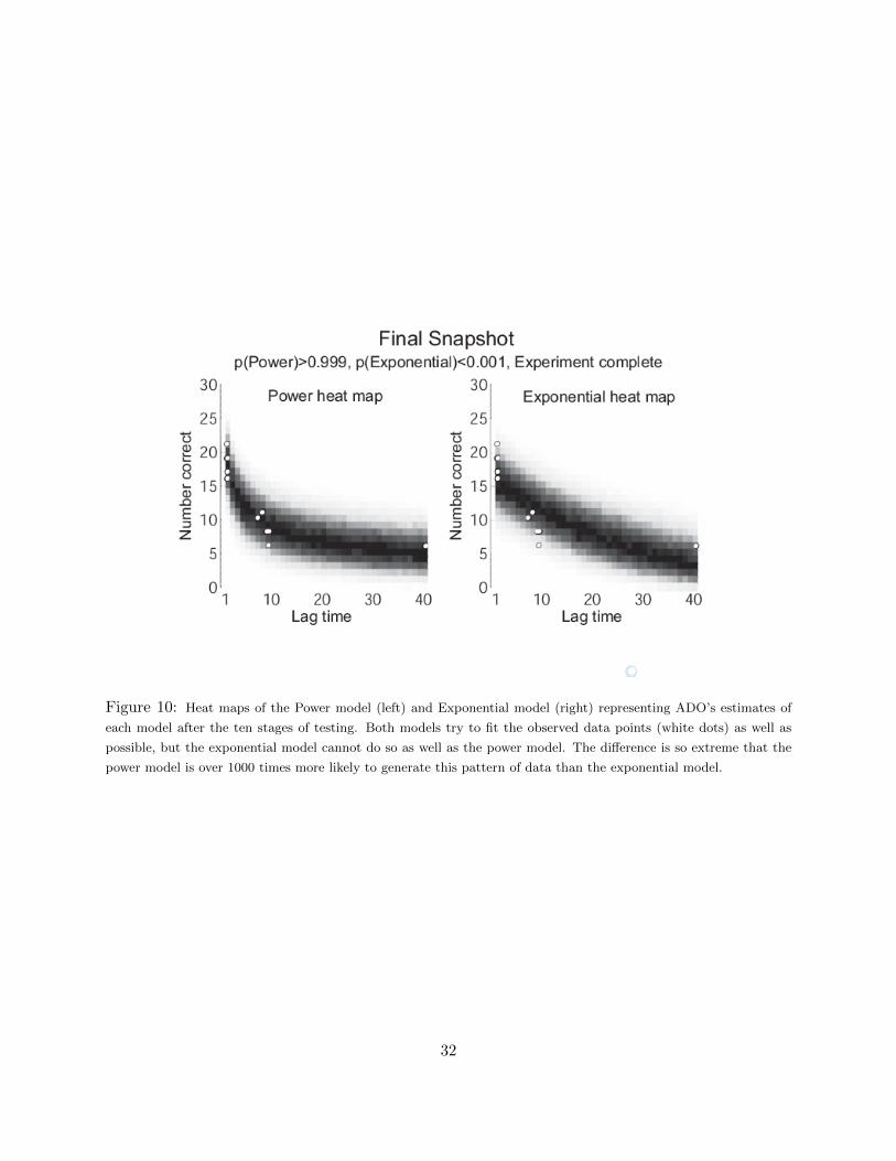
The simulation continued for ten ADO stages. In a real experiment, the experimentercould review a snapshot like Figure 9 after each stage in order to monitor the progress of theexperiment. The experimenter could also add a human element to the design process by choosinga different design than that recommended by ADO for the next stage. For now, we will skip to asnapshot of the experiment after all ten stages have been completed. In Figure 10, the blue dotsrepresent the ten data points that were observed, and the heat maps represent the best estimatesof each model based on those ten data points. It is clear from the heat maps that the exponentialmodel can not match the observed data pattern well, even at its best fitting parameters. On theother hand, the power model can fit the data perfectly (as it should, since it generated the data).Accordingly, the posterior probability of the power model is greater than 0.999, indicating that the

5For a more complex design space (e.g., sets of 3 jointly optimal lag times) one would need to use a more advancedsearch algorithm such as the SMC search described in Section 3.5.2. For example, Cavagnaro et al. (2009) used SMCto find jointly optimal sets of three lag times in each stage of testing in their implementation of ADO in a retentionexperiment.

17

data clearly identify it as the data generating model. Moreover, the heat map estimate of the powermodel closely resembles the heat map of the data-generating model in Figure 7, indicating thatthe parameters have converged to the correct values. Figure 11 shows a typical posterior modelprobability curve obtained from the ADO simulation experiment.

5 Limitations

While ADO has the potential to significantly improve the efficiency of data collection in psycho-logical sciences, it is important that the reader is aware of the assumptions and limitation of themethodology. First of all, not all design variables in an experiment can be optimized in ADO. Theymust be quantifiable in such a way that the likelihood function depends explicitly on the values ofthe design variables being optimized (Myung and Pitt, 2009, p. 511). Consequently, ADO is notapplicable to variables such as type of experimental task (word reading vs. lexical decision) andnominal variables (e.g., words vs. pictures). No statistical methodology currently exists that canhandle such non-quantitative design variables.

Another limitation of the ADO methodology is the assumption that one of the modelsunder consideration is the true, data-generating model. This assumption, obviously, is likely to beviolated in practice, given that our models are merely imperfect representations of the real processunder study.6 Ideally, one would like to optimize an experiment for an infinite array of modelsrepresenting a whole spectrum of realities; no implementable methodology currently exists thatcan handle the problem of this scope.

The ADO algorithm is myopic in the sense that the optimization at each stage of exper-imentation is performed as if the current experiment is the last one to be conducted. In reality,however, the global optimality of the current designs depend upon the outcomes of future experi-ments, as well as those of the previous experiments. This sequential dependency of optimal designsis not considered in the present ADO algorithm, due to the huge computational resources neededto take into account the effect. Recent advances in approximate dynamic programming offers apotentially promising solution to overcome this challenge (e.g., Powell, 2007).

Perhaps the most challenging problem is extending the ADO framework to a class ofsimulation-based models (e.g., Reder et al., 2000; Polyn et al., 2009) that are defined in termsof a series of steps to be simulated on computer without explicit forms of likelihood functions –a prerequisite to implement the current ADO algorithm. Given the popularity of these types ofmodels in cognitive science, ADO will need to be expanded to accommodate them, perhaps usinga likelihood-free inference scheme known as Approximate Bayesian Computation (e.g., Beaumontet al., 2009; Turner and Van Zandt, 2012).

6 Conclusions

In this article, we provided a tutorial exposition of adaptive design optimization (ADO). ADOallows users to intelligently choose experimental stimuli on each trial of an experiment in orderto maximize the expected information gain provided by each outcome. We began the tutorial by

6A violation of this assumption, however, may not be critical in light of the predictive interpretation of Bayesianinference. That is, it has been shown that the model with the highest posterior probability is also the one withthe smallest accumulative prediction error even when none of the models under consideration is the data-generatingmodel (Kass and Raftery, 1995; Wagenmakers et al., 2006; van Erven et al., 2012).

18

contrasting ADO against the traditional, non-adaptive heuristic approach to experimental design,then presented the nuts and bolts of the practical implementation of ADO, and finally, illustratedan application of the experimental technique in simulated experiments to discriminate between tworetention models.

Use of ADO requires becoming comfortable with a different style of experimentation. Al-though the end goal, whether it be parameter estimation or model discrimination, is the same astraditional methods, how you get there differs. The traditional method is a group approach thatemphasizes seeing through individual differences to capture the underlying regularities in behavior.This is achieved by ensuring stable performance (parameters) through random and repeated pre-sentation of stimuli and testing sufficient participants (statistical power). Data analysis comparesthe strength of the regularity against the amount of noise contributed by participants. There isno escaping individual variability, so ADO exploits it by presenting a stimulus whose informationvalue is likely to be greatest for that given participant and trial, as determined by optimizationof an objective function. This means that each participant will likely receive a different subset ofthe stimuli. In this regard, the price of using ADO is some loss of control over the experiment;the researcher turns over stimulus selection to the algorithm, and places faith in it to achieve thedesired ends. The benefit is a level of efficiency that cannot be achieved without the algorithm. Inthe end, it is the research question that should drive choice of methodology. ADO has many uses,but at this point in its evolution, it would be premature to claim it is always superior.

In conclusion, the advancement of science depends upon accurate inference. ADO, thoughstill in its infancy, is an exciting new tool that holds considerable promise in improving inference.By combining the predictive precision of the computational models themselves and the power ofstate of the art statistical computing techniques, ADO can make experimentation informative andefficient, thereby making the tool attractive on multiple fronts. ADO takes full advantage of thedesign space of an experiment by probing repeatedly, in each stage, those locations (i.e., designs)that should be maximally informative about the model(s) under consideration. In time-sensitiveand resource-intensive situations, ADO’s efficiency can reduce the cost of equipment and personnel.This potent combination of informativeness and efficiency in experimentation should acceleratescientific discovery in cognitive science and beyond.

Acknowledgments

This research is supported by National Institute of Health Grant R01-MH093838 to J.I.M andM.A.P. The C++ code for the illustrative example is available upon request from authors. Corre-spondence concerning this article should be addressed to Jay Myung, Department of Psychology,Ohio State University, 1835 Neil Avenue, Columbus, OH 43210. Email: myung.1@osu.edu.

References

Akaike, H. (1973). Information theory and an extension of the maximum likelihood principle. InPetrov, B. N. and Caski, F., editors, Proceedings of the Second International Symposium onInformation Theory, pages 267–281, Budapest. Akademiai Kiado.

Amzal, B., Bois, F., Parent, E., and Robert, C. (2006). Bayesian-optimal design via interactingparticle systems. Journal of the American Statistical Association, 101(474):773–785.

19

Andrieu, C., DeFreitas, N., Doucet, A., and Jornan, M. J. (2003). An introduction to MCMC formachine learning. Machine Learning, 50:5–43.

Atkinson, A. and Donev, A. (1992). Optimum Experimental Designs. Oxford University Press.

Atkinson, A. and Federov, V. (1975). Optimal design: Experiments for discriminating betweenseveral models. Biometrika, 62(2):289.

Beaumont, M. A., Cornuet, J.-M., Marin, J.-M., and Robert, C. P. (2009). Adaptive approximateBayesian computation. Biometrika, 52:1–8.

Bellman, R. E. (2003). Dynamic Programming (reprint edition). Dover Publications, Mineola, NY.

Berry, D. A. (2006). Bayesian clinical trials. Nature Reviews, 5:27–36.

Bolte, A. and Thonemann, U. W. (1996). Optimizing simulated annealing schedule with generticprogramming. European Journal of Operational Research, 92:402–416.

Box, G. and Hill, W. (1967). Discrimination among mechanistic models. Technometrics, 9:57–71.

Burnham, K. P. and Anderson, D. R. (2010). Model Selection and Multi-Model Inference: APractical Information-Theoretic Approach (2nd edition). Springer, New York, NY.

Carlin, H. P. and Louis, T. A. (2000). Bayes and empirical Bayes methods for data analysis, 2nded. Chapman & Hall.

Cavagnaro, D., Gonzalez, R., Myung, J., and Pitt, M. (2013a). Optimal decision stimuli for riskychoice experiments: An adaptive approach. Management Science, 59(2):358–375.

Cavagnaro, D., Pitt, M., Gonzalez, R., and Myung, J. (2013b). Discriminating among probabilityweighting functions using adaptive design optimization. Journal of Risk and Uncertainty, inpress.

Cavagnaro, D., Pitt, M., and Myung, J. (2011). Model discrimination through adaptive experi-mentation. Psychonomic Bulletin & Review, 18(1):204–210.

Cavagnaro, D. R., Myung, J. I., Pitt, M. A., and Kujala, J. V. (2010). Adaptive design optimization:A mutual information based approach to model discrimination in cognitive science. NeuralComputation, 22(4):887–905.

Cavagnaro, D. R., Pitt, M. A., and Myung, J. I. (2009). Adaptive design optimization in experi-ments with people. Advances in Neural Information Processing Systems, 22:234–242.

Chaloner, K. and Verdinelli, I. (1995). Bayesian experimental design: A review. Statistical Science,10(3):273–304.

Cobo-Lewis, A. B. (1997). An adaptive psychophysical method for subject classification. Perception& Psychophysics, 59:989–1003.

Cohn, D., Atlas, L., and Ladner, R. (1994). Improving generalization with active learning. MachineLearning, 15(2):201–221.

20

Cohn, D., Ghahramani, Z., and Jordan, M. (1996). Active learning with statistical models. Journalof Artificial Intelligence Research, 4:129–145.

Cover, T. and Thomas, J. (1991). Elements of Information Theory. John Wiley & Sons, Inc.

Doucet, A., de Freitas, N., and Gordon, N. (2001). Sequential Monte Carlo Methods in Practice.Springer.

Gelman, A., Carlin, J., Stern, H., and Rubin, D. (2004). Bayesian Data Analysis. Chapman &Hall.

Gill, J. (2007). Bayesian Methods: A Social and Behavioral Sciences (2nd edition). Chapman andHall/CRC, New York, NY.

Grunwald, P. D. (2005). A tutorial introduction to the minimum description length principle. InGrunwald, P., Myung, I. J., and Pitt, M. A., editors, Advances in Minimum Description Length:Theory and Applications. The M.I.T. Press.

Hambleton, R. K., Swaminathan, H., and Rogers, H. J. (1991). Fundamentals of Item ResponseTheory. Sage Publications, Newbury Park, CA.

Jeffreys, H. (1961). Theory of Probability. Oxford University Press, Oxford, UK.

Kass, R. E. and Raftery, A. E. (1995). Bayes factors. Journal of the American Statistical Associa-tion, 90:773–795.

Kass, R. E. and Wasserman, L. (1996). The selection of prior distributions by formal rules. Journalof the American Statistical Association, 91(435):1343–1370.

Kirkpatrick, S., Gelatt, C., and Vecchi, M. (1983). Optimization by simulated annealing. Science,220:671–680.

Kontsevich, L. L. and Tyler, C. W. (1999). Bayesian daptive estimation of psychometric slope andthreshold. Vision Research, 39:2729–2737.

Kreutz, C. and Timmer, J. (2009). Systems biology: Experimental design. FEBS Journal, 276:923–942.

Kruschke, J. K. (2010). Doing Bayesian Data Analysis: A Tutorial with R and BUGS. AcademiCPress, New York, NY.

Kujala, J. and Lukka, T. (2006). Bayesian adaptive estimation: The next dimension. Journal ofMathematical Psychology, 50(4):369–389.

Lesmes, L., Jeon, S.-T., Lu, Z.-L., and Dosher, B. (2006). Bayesian adaptive estimation of thresholdversus contrast external noise functions: The quick TvC method. Vision Research, 46:3160–3176.

Lesmes, L., Lu, Z.-L., Baek, J., and Dosher, B. (2010). Bayesian adaptive estimation of the contrastsensitivity function: The quick SCF method. Journal of Vision, 10:1–21.

Lewi, J., Butera, R., and Paninski, L. (2009). Sequential optimal design of neurophysiology exper-iments. Neural Computation, 21:619–687.

21

Lindley, D. (1956). On a measure of the information provided by an experiment. Annals ofMathematical Statistics, 27(4):986–1005.

Loredo, T. J. (2004). Bayesian adaptive exploration. In Erickson, G. J. and Zhai, Y., editors,Bayesian Inference and Maximum Entropy Methods in Science and Engineering: 23rd Interna-tional Workshop on Bayesian Inference and Maximum Entropy Methods in Science and Engi-neering, volume 707, pages 330–346. American Institute of Physics.

Muller, P. (1999). Simulation-based optimal design. In Berger, J. O., Dawid, A. P., and Smith,A. F. M., editors, Bayesian Statistics, volume 6, pages 459–474, Oxford, UK. Oxford UniversityPress.

Muller, P., Sanso, B., and De Iorio, M. (2004). Optimal Bayesian design by inhomogeneous Markovchain simulation. Journal of the American Statistical Association, 99(467):788–798.

Myung, J. I. and Pitt, M. A. (2009). Optimal experimental design for model discrimination.Psychological Review, 58:499–518.

Nelson, J. (2005). Finding useful questions: On Bayesian diagnosticity, probability, impact, andinformation gain. Psychological Review, 112(4):979–999.

Nelson, J., McKenzie, C. R. M., Cottrell, G. W., and Sejnowski, T. J. (2011). Experience matters:Information acquisition optimizes probability gain. Psychological Science, 21(7):960–969.

Oberauer, K. and Lewandowsky, S. (2008). Forgetting in immediate serial recall: Decay, temporaldistinctiveness, or interference? Psychological Review, 115(3):544–576.

Pitt, M. A., Myung, I. J., and Zhang, S. (2002). Toward a method of selecting among computationalmodels of cognition. Psychological Review, 190(3):472–491.

Polyn, S. M., Norman, K. A., and Kahana, M. J. (2009). A context maintenance and retrievalmodel of organizational processes in free recall. Psychological Review, 116:129–156.

Powell, W. B. (2007). Approximate Dynamic Programming: Solving the Curses of Dimensionality.John Wiley & Sons, Hoboken, New Jergey.

Reder, L. M., Nhouyvanisvong, A., Schunn, C. D., Avyers, M. S., Angstadt, P., and Hiraki, K.(2000). A mechanistic account of the mirror effect for word frequency: A computational modelof remember-know judgments in a continuous recognition paradigm. Journal of ExperimentalPsychology: Learning, Memory and Cognition, 26:294–320.

Rissanen, J. (1978). Modeling by shortest data description. Automatica, 14:461–471.

Robert, C. P. (2001). The Bayesian Choice: From Decision-Theoretic Foundations to Computa-tional Implementation (2nd edition). Springer, New York, NY.

Robert, C. P. and Casella, G. (2004). Monte Carlo Statistical Methods (2nd edition). Springer,New York, NY.

Rubin, D. and Wenzel, A. (1996). One hundred years of forgetting: A quantitative description ofretention. Psychological Review, 103(4):734–760.

22

Sutton, R. S. and Barto, A. G. (1998). Reinforcement Learning: An Introduction. MIT Press,Cambridge, Massachusetts.

Tang, Y., Young, C., Myung, J. I., Pitt, M. A., and Opfer, J. (2010). Optimal inference andfeedback for representational change. In Ohlsson, S. and Catrambone, R., editors, Proceedingsof the 32nd Annual Meeting of the Cognitive Science Society, pages 2572–2577, Austin, TX.Cognitive Science Society.

Turner, B. and Van Zandt, T. (2012). A tutorial on approximate bayesian computation. Journalof Mathematical Psychology, 56(2):69–85.

van der Linden, W. J. and Glas, C. A. W. (2000). Computerized Adaptive Testing. Kluwer AcademicPublishers, Boston, MA.

van Erven, T., Grunwald, P. D., and de Rooji, S. (2012). Catching up faster by switching sooner:A predictive approach to adaptive estimation with an application to the AIC-BIC Dilemma.Journal of the Royal Statistical Society, Series B, 74:361–397.

Vul, E. and Bergsma, J. MacLeod, I. A. (2010). Functional adaptive sequential testing. Seeing andPerceiving, 23:483–513.

Wagenmakers, E.-J., Grunwald, P. D., and Steyvers, M. (2006). Accumulative prediction error andthe selection of time series models. Journal of Mathematical Psychology, 50:149–166.

Wathen, J. K. and Thall, P. F. (2008). Bayesian adaptive model selection for optimizing groupsequential clinical trials. Statistics in Medicine, 27:5586–5604.

Weiss, D. J. and Kingsbury, G. G. (1984). Application of computerized adaptive testing to educa-tional problems. Journal of Educational Measurement, 21:361–375.

Wixted, J. and Ebbesen, E. (1991). On the form of forgetting. Psychological Science, 2(6):409–415.

23

Figure 1: Sample power (POW) and exponential (EXP) functions, generated from a narrow range of model pa-

rameters (see text). The time intervals between 1 and 5 seconds, where the models are the most discriminable, are

indicated by the blue circles. In contrast, the green elliptic circles indicate the time intervals (i.e., 15 - 20 seconds)

that offer the least discriminability.

24

Figure 2: Schematic illustration of the traditional experimentation versus adaptive experimentation paradigm.

(a) The vertical arrow on the left represents optimization of the values of design variables before data collection.

The vertical arrow on the right represents the analysis and modeling of the data collected, using model selection

or parameter estimation methods, for example. (b) In the adaptive experimentation paradigm, the three parts of

experimentation (design optimization, experiment, and data modeling) are closely integrated to form a cycle of

inference steps in which the output from one part is fed as an input to the next part.

25

Figure 3: Schematic illustration of the steps involved in adaptive design optimization (ADO).

26

Grid Search

• Initialize positive integers M and N, and a Mx1 vector U = 0

• for 1 ≤ g ≤M do

• Select the g-th design point, dg, from the discretized design space

• for 1 ≤ i ≤ N do

• Sample model index k(i) from the model prior p(m)

• Sample parameter θk(i)(i) from the parameter prior p(θk(i))

• Sample data yk(i)(i) from the probability distribution p(yk(i)|θk(i)(i), dg)

• Calculate u(dg, θk(i)(i), yk(i)(i)

)• Set U(g)← U(g) + u

(dg, θk(i)(i), yk(i)(i)

)/N

• end for

• end for

• Identify optimal design d∗ as the design associated with maxg

U(g)

Figure 4: The grid search algorithm.

27

Figure 5: Illustration of sequential Monte Carlo search design optimization with simulated annealing.

28

Sequential Monte Carlo (SMC) Search

• Given a simulated annealing schedule function ρ(t), a peakedness measure

δ(S), and a threshold ε (> 0):

• Initialize N, I = 1, and δ(S) = 0

• While δ(S) < ε do

• Set J ← ρ(I)

• Use an SMC sampling procedure to generate a sample S of N random

• draws, {d, {m}, {ym}, {θm}}’s, from the auxiliary distribution h(·)J

• Evaluate δ(S)

• Set I ← I + 1

• end while

• Identify optimal design d∗ as the mean (or alternatively, median or mode)

of all d’s in the current sample S

Figure 6: The SMC search algorithm.

29

1

Figure 7: Heat map of the data-generating model in the ADO simulation. Darker colors indicate regions of higher

probability.

30

Figure 8: Heat maps of the Power model (left) and Exponential model (right) representing ADO’s prior estimates

of each model. Darker colors indicate regions of higher probability. The lag time of t = 7 (blue rectangle) is chosen

for testing in the first stage because it is the place where the two models differ the most, based on the priors.

Figure 9: Heat maps of the Power model (left) and Exponential model (right) representing ADO’s estimates of

each model after the first stage of testing (prior to the second stage). Estimates have converged around the observed

data point (white dot in each heat map). ADO selects t = 1 (blue rectangle) for testing in Stage 2 because it is the

place where the two models differ the most, based on these updated estimates.

31

Figure 10: Heat maps of the Power model (left) and Exponential model (right) representing ADO’s estimates of

each model after the ten stages of testing. Both models try to fit the observed data points (white dots) as well as

possible, but the exponential model cannot do so as well as the power model. The difference is so extreme that the

power model is over 1000 times more likely to generate this pattern of data than the exponential model.

32

Figure 11: Posterior model probability curve from a sample run of the ADO simulation experiment. The data were

generated from the power model with parameters a = 0.80 and b = 0.40. See the text for additional details of the

simulation.

33