1 Absolute Calibration of ATMS Upper Level Temperature Sounding Channels Using GPS RO Observations Xiaolei Zou 1,2∗ , Lin Lin 3,4 , and Fuzhong Weng 5 1 Center of Data Assimilation for Research and Application, Nanjing University of Information and Science & Technology, Nanjing, China 2 Deptment of Earth, Ocean and Atmospheric Sciences, Florida State University, USA 3 Joint Center for Satellite Data Assimilation, College Park, Maryland, USA 4 Earth Resources Technology, Inc. Laurel, Maryland, USA 5 National Environmental Satellite, Data, & Information Service, National Oceanic and Atmospheric Administration, Washington, D. C., USA IEEE Trans. Geosci. Remote Sens. September 2012 ∗ Corresponding author: Dr. X. Zou, Department of Earth, Ocean and Atmospheric Science, Florida State University, Tallahassee, FL 32306-4520, USA. Email: [email protected]. Phone: 850-644-6025.
Transcript
1
Absolute Calibration of ATMS Upper Level Temperature
Sounding Channels Using GPS RO Observations
Xiaolei Zou1,2∗, Lin Lin3,4, and Fuzhong Weng5
1Center of Data Assimilation for Research and Application, Nanjing University of
Information and Science & Technology, Nanjing, China
2Deptment of Earth, Ocean and Atmospheric Sciences, Florida State University, USA
3Joint Center for Satellite Data Assimilation, College Park, Maryland, USA
4Earth Resources Technology, Inc. Laurel, Maryland, USA
5National Environmental Satellite, Data, & Information Service, National Oceanic and
Atmospheric Administration, Washington, D. C., USA
IEEE Trans. Geosci. Remote Sens.
September 2012
∗Corresponding author: Dr. X. Zou, Department of Earth, Ocean and Atmospheric Science, Florida State University, Tallahassee, FL 32306-4520, USA. Email: [email protected]. Phone: 850-644-6025.
2
Abstract
The absolute accuracy of antenna brightness temperatures (TDR) from the Advanced Technology
Microwave Sounder (ATMS) onboard the Suomi National Polar-orbiting Partnership (NPP)
satellite is estimated using Constellation Observing System for Meteorology, Ionosphere, and
Climate (COSMIC) Radio Occultation (RO) data as input to the U.S. Joint Center of Satellite
Data Assimilation (JCSDA) Community Radiative Transfer Model (CRTM). It is found that the
mean differences (e.g., biases) of observed TDR observations to GPS RO simulations are
positive for channels 6, 10-13 with values smaller than 0.5K and negative for channels 5, 7-9
with values greater than -0.7K. The bias distribution is slightly asymmetric across the scan line.
A line-by-line radiative transfer model is used to further understand the sources of errors in
forward calculations. It is found that for some channels, the bias can be further reduced in a
magnitude of 0.3K if the accurate line-by-line simulations are used. With the high quality of GPS
RO observations and the accurate radiative transfer model, ATMS upper level temperature
sounding channels are calibrated with known absolute accuracy. After the bias removal in ATMS
TDR data, it is shown that the distribution of residual errors for ATMS channels 5-13 is close to
a normal Gaussian one. Thus, for these channels, the ATMS antenna brightness temperature can
be absolutely calibrated to the sensor brightness temperature without a systematic bias.
3
1. Introduction
The Suomi National Polar-orbiting Partnership (SNPP) satellite is the pathfinder in
building up the next-generation satellite system that will take over NASA’s Earth Observing
System (EOS) satellites launched in the last decade. It was successfully launched on October 28,
2011 from Vandenberg Air Force Base, California. The Advanced Technology Microwave
Sounder (ATMS) is one of the five key instruments onboard SNPP and is the heritage of
Advanced Microwave Sounding Unit-A (AMSU-A) and Microwave Humidity Sounder (MHS)
combined. AMSU-A and MHS are two crossing-scanning microwave radiometers onboard the
past National Oceanic and Atmospheric Administration (NOAA) and European polar-orbiting
satellites (e.g., NOAA-15, -16, -17, -18, -19, MetOp-A, -B). Compared with AMSU-A and
MHS, ATMS has more channels, wider scan swath, overlapping field-of-view (FOV) sampling
and higher spatial resolution temperature sounding channels than AMSU-A (Weng et al., 2012a).
Soon after the launch of SNPP, ATMS on-orbit performance had been well characterized,
channel noise and accuracy had exceeded the mission requirements, the ATMS data have been
archived on NOAA’s Comprehensive Large Array data Stewardship System (CLASS) and can
be accessed by the broad user community.
Radiation at microwave frequencies emitted from atmospheric constituents such as oxygen
allows for remote sensing of the atmospheric temperature. Through a two-point calibration
equation (Mo, 1996; Zou et al., 2011), the signal from the microwave radiometer can be linked to
the brightness temperature. In ATMS calibration, the biases are expected in radiance
measurements due to many calibration error sources. For example, biases could also come from
spacecraft emission, earth-view side lobe effects, and atmospheric inhomogeneity. The later
often causes a scan-dependent bias feature for a cross-track scanning radiometer (Weng et al.,
4
2012b). It is important to quantify, document and correct these data biases before their
applications in weather and climate predictions. This study investigates bias characteristics in
ATMS data and proposes an absolute post-launch calibration algorithm using GPS RO data,
which is SI-traceable.
Similar to satellite passive microwave instruments such as AMSU-A, calibrations of
ATMS antenna brightness temperatures (TDR) data also lack the traceability to International
Standard (SI) units. It is important to assess the instrument in-orbit accuracy for both NWP and
climate applications. The Global Positioning System (GPS) Radio Occultation (RO) raw data are
in principle SI traceable and have high accuracy and precision, high vertical resolution, no
contamination from clouds, no system calibration required, and no instrument drift (Rocken et al.
1997; Anthes et al. 2000; Lin et al. 2010; Yang and Zou, 2012). In addition, the atmospheric
radiative transfer models (RTMs) are very accurate for ATMS upper-troposphere and low
stratosphere temperature sounding channels. These unique features of GPS ROs and RTMs make
it possible to derive the in-orbit absolute calibration of ATMS upper-level temperature sounding
channels 5-13. The CRTM simulations with GPS RO data as its input can be used for
characterizing the statistical features of ATMS data from the post-launch in-orbit performance of
the ATMS instrument.
An improved characterization of ATMS performance would also benefit the climate
research using long-term climate data records (CDRs) consisting of observations from
operational polar-orbiting satellite systems. ATMS inherited most of the sounding channels from
its heritage predecessors: Advanced Microwave Sounding Unit-A (AMSU-A) and Microwave
Humidity Sounder (MHS) onboard NOAA-15, NOAA-16, NOAA-17, NOAA-18 and NOAA-19
and MetOp-A satellites since 1998, and all four channels of the Microwave Sounding Unit
5
(MSU) onboard the early NOAA satellites from Tiros-N through NOAA-14 from 1979 to 2007.
Therefore, there are nearly 35 years of four MSU channels global satellite data. MSU/AMSU-A
brightness temperature observations were widely used by the community for climate studies
(Christy et al., 1998, 2000, 2003; Mears et al., 2003, Mears and Wentz, 2009; Vinnikov and
Grody, 2007; and Zou et al., 2009). With ATMS onboard Suomi NPP, the MSU/AMSU time
series can be further extended. Since a much more refined post-launch calibration is required to
deduce long-term climate trend with adequate accuracy, precision, stability and consistency
(Ohring et al., 2005), this study could also contributes to future integration of ATMS data into
long-term satellite CDRs.
As the first step of an in-orbit absolute calibration of ATMS data, this study aims at
assessing the bias for ATMS upper level sounding channels using collocated GPS RO data.
Sections 2-4 will briefly discuss the ATMS instrument characteristics, the Constellation
Observing System for Meteorology, Ionosphere, and Climate/Formosa Satellite Mission 3
(COSMIC/FORMOSAT3, hereafter referred to as COSMIC for brevity) RO data, and the
radiative transfer models used in this study. Section 5 discusses the collocation method. ATMS
upper level sounding channel biases are estimated in Section 6 using fast radiative transfer
model. Section 7 compares accuracy of the line-by-line ATMS brightness temperature
simulations using laboratory-measured and BoxCar-approximated spectral response functions.
Summary and conclusions are provided in Section 8.
2. A Brief Description of ATMS Instrument
The carrier of ATMS, Suomi NPP, is rotating around the Earth on a circular, 98.7o
inclination orbit at 824-km altitude. ATMS is a total-power, 22 channel passive microwave
sounder with the scan angular span of ±52.77o relative to nadir. A total of 96 field-of-view
6
(FOV) samples are taken along each scan line, and each FOV sample represents the mid-point of
a sampling interval of about 18ms. Two receiving antennas are installed on the ATMS sensor,
one is for channels 1-15 with frequencies below 60 GHz and the other is for channels 16-22 with
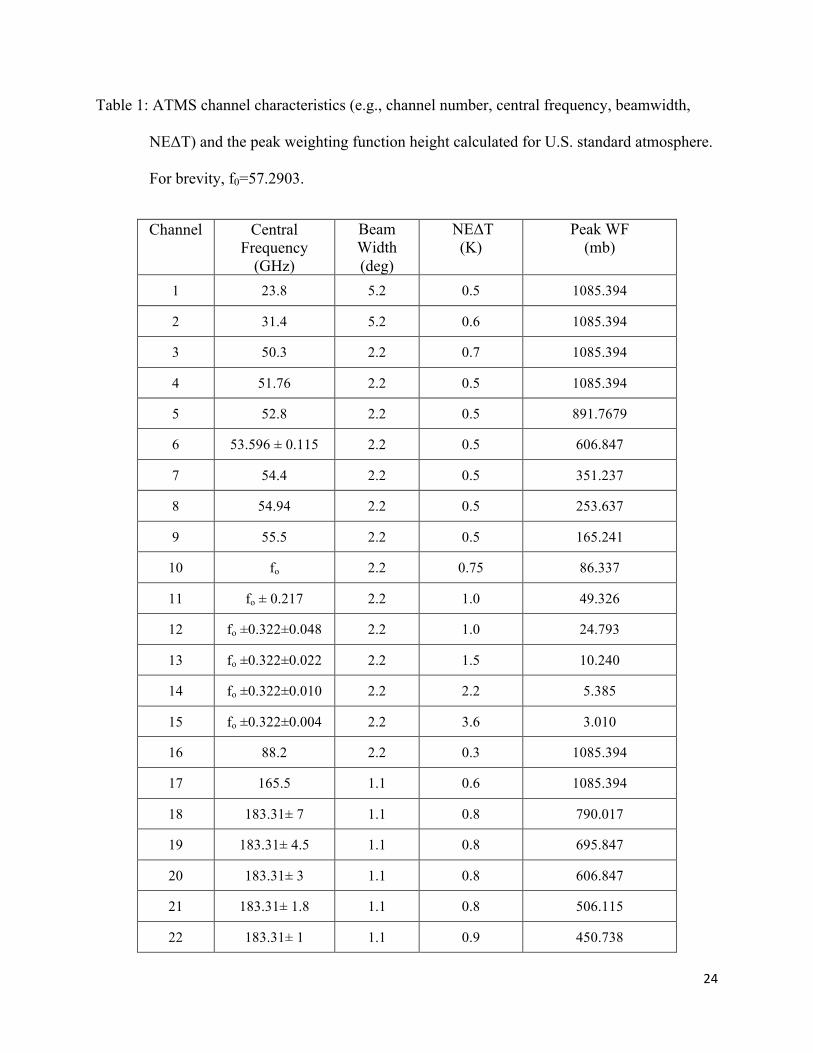
frequencies above 60 GHz. The beam width is 5.2o for channels 1-2, 2.2o for channels 3-16 and
1.1o for channels 17-22 (Table 1). ATMS provides both temperature soundings within the
surface to the upper stratosphere (about 1hPa, ~45km), and humidity soundings within the
surface to upper troposphere (about 200hPa, ~15km).
The antenna reflectors continuously rotate counter-clockwise relative to the spacecraft
direction of motion, completing three revolutions in eight seconds. Each scan cycle is divided
into three segments. In the first segment, the Earth is viewed at 96 different angles, symmetric
around the nadir direction. The angular range between the first and the last sample centroids is
105.45o. The antenna then accelerates and moves to a position that points toward an unobstructed
space view (i.e., between the Earth’s limb and the spacecraft horizon). It then resumes the same
scan speed as maintained across the Earth scenes while four consecutive cold calibration
measurements are taken. Next, the antenna is accelerated to move toward the zenith direction,
points toward an internal calibration target that is at the relatively high ambient instrument
temperature, and resumes the normal scan speed while four consecutive warm calibration
measurements are taken. Finally, it is accelerated to the starting position viewing the Earth scene,
where it is slowed down to normal scan speed to begin another scan cycle.
3. A Brief Description of COSMIC RO Data
The GPS RO is a limb-sounding technique that makes use of radio signals emitted from the
GPS satellites for sounding Earth’s atmosphere. Under the assumption of the spherical symmetry
of the atmospheric refractive index, vertical profiles of bending angle and refractivity can be
7
derived from the raw RO measurements of the excess Doppler shift of the radio signals
transmitted by GPS satellites (see Appendix A1 in Zou et al. 1999). The profiles of refractivity
are then used to generate profiles of the temperature and water vapor retrieval using a one-
dimensional variational data assimilation (1D-Var) algorithm (Healy and Eyre, 2000; Palmer et
al. 2000). The CDAAC wet retrieval is used in this study. A brief description of a 1D-Var
algorithm for GPS RO retrieval is provided at http://cosmic-
io.cosmic.ucar.edu/cdaac/doc/documents/1dvar.pdf.
The COSMIC satellite system consists of a constellation of six low-Earth-orbit (LEO)
microsatellites, and was launched on April 15, 2006. Each LEO follows a circular orbit 512 km
above the Earth surface, with an inclination angle of 72o. Currently, there are about 1000
soundings daily. The vertical resolution is 0.1km from surface to 39.9 km, and each GPS RO
measurement quantifies an integrated atmospheric refraction effect over a few hundred
kilometers along a ray path centered at the tangent point. The global mean differences between
COSMIC and high-quality reanalysis within the height range between 8 and 30 km are estimated
to be ~0.65K (Kishore et al. 2008). The precision of COSMIC GPS RO soundings, estimated by
comparison of closely collocated COSMIC soundings, is approximately 0.05K in the upper
troposphere and lower stratosphere (Anthes et al. 2008). In the water vapor abundant region in
the lower troposphere (e.g., when temperature is greater than 270K), the precision reduces to
about 0.1K. In the ionosphere regions, GPS profiles become less accurate due to residual
ionospheric effect. The estimated precision of COSMIC GPS RO soundings is approximately
0.2K in the ionosphere.
4. Radiative Transfer Models
4.1 CRTM
8
CRTM stands for Community Radiative Transfer Model and is developed and distributed
by the US Joint Center for Satellite Data Assimilation (JCSDA). The model is publicly available
and may be downloaded from ftp://ftp.emc.ncep.noaa.gov/jcsda/CRTM/REL-2.0.5/. The CRTM
is a sensor-channel-based radiative transfer model (Han et al. 2006; Weng et al. 2007; Han et al.
2010) and is widely used for microwave and infrared satellite data assimilation and remote
sensing applications. It includes modules that compute the satellite-measured thermal radiation
from gaseous absorption, absorption and scattering of radiation by aerosols and clouds, and
emission and reflection of radiation by the Earth surface. The input to the CRTM includes
atmospheric state variables (temperature, water vapor, pressure, and ozone concentration at user
defined layers, and optionally, liquid water content and mean particle size profiles for up to six
cloud types), and surface state variables and parameters including the surface emissivity, surface
skin temperature, and surface wind. In addition to CRTM (i.e., the forward model), the
corresponding tangent-linear, adjoint, and K-matrix models have also been included in the
CRTM package.
In this study, the vertical profiles of temperature, water vapor and pressure are obtained
directly from COSMIC GPS RO retrieval. The mixing ratio profile of ozone is set to be equal to
the U.S. standard atmospheric state. For simplicity, no cloud or aerosols are considered in the
radiative transfer simulation. The emissivity is derived from the CRTM oceanic surface model
at microwave frequencies.
4.2 MonoRTM
The Atmospheric and Environmental Research (AER) Inc. Monochromatic Radiative
Transfer Model (MonoRTM) is an accurate line-by-line RTM for use in the microwave region. It
employs an accurate atmospheric spectroscopy database and only considers gaseous absorption.
9
A detailed description of MonoRTM physics can be found in Clough et al. (2005) and Payne et
al. (2011). Figure 1 shows the amount of contributions of different atmospheric constituents in
the microwave region, which is calculated using MonoRTM for a U.S. standard atmosphere.
Between 50-70 GHz, O2 is the only absorption gas. By including the fine absorption line (Fig.
1b), MonoRTM accurately simulates the ATMS microwave sounding channels within 50-70
GHz O2 absorption band through a line-by-line calculation procedure. In this study, MonoRTM
version 4.2 is used. Input to MonoRTM is the same as that for CRTM, i.e., the vertical profiles of
temperature, water vapor and pressure from COSMIC GPS RO retrieval.
5. Collocation between GPS RO and ATMS
In the present study, COSMIC RO soundings collocated with ATMS measurements are
selected for assessing the accuracy of ATMS measurements. The collocation criteria are set by a
time difference of no more than three hours and a horizontal spatial separation of less than 50 km
at the altitude of peak weight function. If there are more than one ATMS pixel measurements
satisfying these collocation criteria, the one that is closest to the related COSMIC sounding is
chosen and others are discarded. Because surface state variables and parameters are not provided
by COSMIC ROs, only upper-level temperature sounding channels are simulated using COSMIC
GPS RO data. The NCEP GFS surface wind field is used in the forward model calculations. The
surface emission variation due to changes in wind speed could contribute to the simulation of
ATMS channel 5. The global biases as well as the angular dependence of biases are estimated.
As the GPS radio signal passes through the atmosphere, its ray path is bent over due to
variations of atmospheric refraction. Therefore, the geolocation of the perigee point (also called
tangent point) of a single RO profile varies with altitude. On the other hand, a satellite
measurement at a specific frequency represents a weighted average of radiation emitted from
10
different layers of the atmosphere. The magnitude of such a weighting is determined by a
channel-dependent weighting function (WF). The measured radiation is most sensitive to the
atmospheric temperature at the altitude where the WF reaches a maximum. The WF also varies
with scan angle (Fig. 2). For each channel, the altitude of the peak WF is the lowest at the nadir
and increases with the scan angle. Considering the geolocation change of the perigee point of a
GPS RO profile with altitude, the geolocation of a GPS RO at the altitude where the WF for each
collocated ATMS FOV of a particular sounding channel reaches the maximum is used for
implementing the spatial collocation criteria of less than 50 km, where the altitude of the
maximum WF is determined by inputting the U.S. standard atmosphere into CRTM (see Table
1).
Based on the fact that the surface emissivity influences vary greatly over land, and the
physical properties of brightness temperature for the sounding channels are affected by clouds, a
cloud detection algorithm similar to Weng et al. (2003) is applied to separate the data in clear-
sky conditions over ocean from total ATMS measurements (Weng et al., 2012a). Figure 3a
presents the spatial distribution of the ATMS observations that are collocated with COSMIC
GPS RO data in clear-sky conditions over ocean and between 60S-60N from December 10, 2011
to June 30, 2012. Most collocated data are located in subtropical in Northern Hemisphere and
middle latitudes in Southern Hemisphere, which is largely determined by the latitudinal
dependence of the ocean area (Fig. 3b). A similar pattern is found for channels 5, 7-13.
6. Bias Estimate and GPS RO Calibration Results
For brevity, model simulations of the ATMS brightness temperatures using GPS RO profiles
as input to CRTM will be denoted BGPS hereafter. The altitudes of the maximum WF of ATMS
channels 14-15 are above 40 km, which is the top of COSMIC RO data. Therefore, biases of
11
ATMS channels 14-15 are not included in this study. Figure 4 presents scatter plots of brightness
temperature from ATMS observations (O) and GPS RO simulations (BGPS) for all collocated data
points under clear-sky conditions over ocean between 60S-60N from December 10, 2011 to June
30, 2012. In general, CRTM simulations with GPS RO input profiles correlate quite well with
ATMS observations. A noticeable temperature dependence of the differences (O-BGPS) between
observations and simulations is seen in channel 6. Global biases estimated by the mean
differences (O-BGPS) are positive for channels 6, 10-13 with values smaller than 0.5K and
negative for channels 5, 7-9 with values greater than -0.7K (Fig. 5). The standard deviation is
smallest for channel 8 (~0.25K), increases with channel number to about 2.0K at channel 13
(Fig. 5). The standard deviations for channels 5 and 6 are 0.4K and 0.6K, respectively.
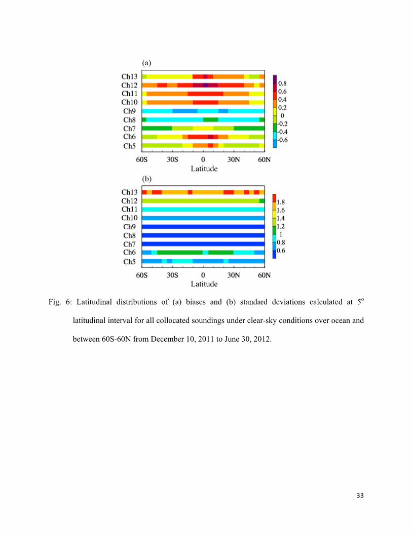
A strong latitudinal dependence of global biases is found for ATMS data (Fig. 6a). Positive
biased for channels 5-6, 10-13 are largest in low latitudes. A weaker latitudinal dependence of
biases is found for ATMS channels 7-9 (Fig. 6a). The standard deviations (Fig. 6b) have a
smaller latitudinal dependence than biases.
For a cross-track scanning radiometer like ATMS, the variation of the optical path length
with scan angle is modeled through CRTM. However, the variation of atmospheric
inhomogeneity with scan angle has not been explicitly simulated in CRTM. In addition, effects
of the spacecraft radiation on brightness temperatures can also vary with scan angle. Therefore, a
scan-angle dependent bias is expected for the cross-track scanning radiometer. In many
applications such as weather predictions through radiance data assimilation, angular-dependent
biases must be properly quantified so that they could be removed before data applications.
Figure 7 presents scan-dependent biases and standard deviations of ATMS channels 5-13
estimated by using GPS RO data. Variations of GPS RO profiles numbers collocated with
12
ATMS data are also shown in Fig. 7. As expected, the total number of collocated GPS ROs
increases with scan angle since the size of FOV increases with scan angle. An asymmetric scan
bias pattern is noticed for ATMS channels 5-10. ATMS temperature sounding channels are more
negatively biased near the ends of ATMS scan lines. The standard deviations of ATMS channels
6, 12 and 13 are much larger than the remaining channels. The root causes of the asymmetric
bias pattern came from the contributions from the near field (e.g., spacecraft) side-lobes, which
were confirmed by using the ATMS pitch maneuver data (Weng et al., 2012b). The closer the
spacecraft temperature is to a channel’s temperature, the less impact of the spacecraft side-lobes
on the scan bias of that channel.
Spatial distributions of the differences of brightness temperature between ATMS
observations and GPS RO simulations (O-BGPS) after the GPS RO absolute post-launch
calibration are much more homogeneously distributed over the globe than those without the GPS
RO absolute post-launch calibration. Figure 8a-b presents frequency distributions of O-BGPS
differences before and after the GPS RO absolute post-launch calibration are plotted for ATMS
channels 5-13 using all collocated data from December 10, 2011 to June 30, 2012 under clear-
sky conditions over ocean within 60S-60N. Monthly variations of biases and standard deviations
of the differences between ATMS observations and GPS RO simulations (O-BGPS) after the GPS
RO absolute post-launch calibration are provided in Fig. 8c. A noticeable difference of the
frequency distribution between Figs. 8a and 8b is in the variation of bias with channel number.
Before GPS RO calibration, the biases with different channels are different. After GPS RO
calibration, all channels assume a nearly normal Gaussian distribution. The only differences
among different channels are the standard deviations. By comparing Fig. 8c with Fig. 5, it is seen
that global biases after the GPS RO calibration are about an order of magnitude smaller than
13
those of the original TDR data. Impacts of GPS RO calibration on the standard deviations are
only slightly reduced. The standard deviations increase fast for upper-level channels 10-13 in a
similar way as their noise equivalent temperature difference (NEΔT) values (see Table 1). The
standard deviations for these channels after GPS calibration (Fig. 8) are only slightly larger than
their NEDT values.
Another noticeable feature from Fig. 8 is that the width of the Gaussian frequency
distribution for an individual channel is reduced after the GPS RO calibration. This is due to the
fact that data from all FOVs are plotted in Fig. 8 while biases for a cross-track microwave
instrument are FOV-dependent. If the Gaussian frequency distribution for a specified FOV is
plotted (Fig. 9), the width of the Gaussian frequency distribution for an individual channel does
not change.
7. MonoRTM Simulations Using Measured and Boxcar Spectral Response Function
In CRTM, the relative spectral response function (SRF) is set as Boxcar, i.e., the relative
SRF uniformly set to equal to one between the band frequency boundaries. For each band, there
are 256 absorption lines. More specifically, if there are two bands or four bands for a certain
channel, the number of lines is 128 and 64 within the second and third sub-band. In March 2012,
the ATMS Pre-Flight Model (PFM) SRF report is provided by Kim and Lyu (2012), in which the
PFM filter digitized SRF data at three base-plate temperatures (-10oC, +20oC and +50oC) and at
low, nominal and high oscillator bias levels are presented. For V, W and G bands, the laboratory
experiments were performed for both primary and secondary local oscillator settings.
With the above-mentioned laboratory-measured SRF, the accuracy of CRTM can be
assessed using the MonoRTM. The top level of the COSMIC GPS RO data is extended from
about 2hPa to 0.005hPa using 1976 US standard atmospheric profile. To save computational
14
time, the SRF is truncated at -20dB to keep the 99% of the maximum SRF for each band of each
channel. Details of the relative SRF before and after the truncations are listed in Table 2.
Compared to 256 lines for Boxcar SRF, the number of lines for truncated measured SRF is at
least tripled for each channel. The ATMS Boxcar and -20dB truncated relative SRF for each
channel are shown in Fig. 10. It is found that the ATMS Boxcar frequency boundary generally
matches with the -20dB truncated SRF quite well for ATMS channels 5-13. The global biases
and standard deviations of the MonoRTM-simulated brightness temperature differences between
the Boxcar and the -20dB-truncated SRF in January 2012 are shown in Fig. 11. We can see the
mean difference is within 0.2K for all channels, which is larger than the data biases after GPS
RO post-launch calibration (Fig. 8c). The standard deviations are also less than 0.2K, which is an
order of magnitude smaller than the standard deviations of O-BGPS. It is thus concluded that for
NWP radiance data assimilation, the forward radiative transfer models should either use the
measured SRFs or remove model biases introduced by using the Boxcar SRF estimated in Fig.
11.
8. Summary and Conclusions
GPS RO observations are very accurate from 2-3 km to about 40 km and are most accurate
between 8 and 30 km, making them ideally suitable for estimating biases of upper level ATMS
temperature sounding channels. In the past seven months from December 10, 2011 to June 30,
2012, COSMIC GPS RO data and ATMS upper-level sounding observations are collocated.
Since the geographical location of a single GPS RO profile could vary for more than a few
hundred kilometers from the top of the atmosphere to the observed lowest altitude, the
collocation between a COSMIC GPS RO profile and a FOV of an ATMS channel is carried out
between the geographical location of both types of data at the ATMS channel peak weighting
15
function altitude. Statistical features of the differences between ATMS observations and GPS
RO simulations for upper-level sounding channels are analyzed using all collocated data under
clear-sky conditions over ocean. The GPS RO simulations are produced by CRTM. Since the
proposed absolute post-launch calibration of ATMS satellite measurements using GPS RO data
relies on CRTM, the model bias of CRTM is estimated. Specifically, biases of different ATMS
channels using the so-called Boxcar SRF that is implemented in CRTM is assessed using an
accurate line-by-line radiative transfer model (e.g., MonoRTM). Comparison of simulations
obtained from using the measured SRF versus the Boxcar SRF shows a CRTM model bias less
than 0.2K. The largest model bias of about 0.18K occurred in ATMS channel 7.
The ATMS global brightness temperature biases are within 0.7K for all channels
examined (e.g., ATMS channels 5-13). The magnitudes of biases vary with channel number. A
small monthly variation of biases is observed. The error distributions are not of normal Gaussian
types. Also, the biases have an asymmetric distribution with respect to scan angle. When such an
asymmetric scan-dependent bias estimated by GPS RO simulation for each individual channel is
removed from the data, the errors of the ATMS sensor data record (SDR) at channels 5-13
becomes a normal Gaussian distribution.
The present study will contribute to the establishment of satellite microwave temperature
sounding climate data record which requires the ATMS data be linked to earlier NOAA polar-
orbiting satellite microwave temperature sounding data (e.g., MSU and AMSU-A). It is noted
that the temperature and water vapor profiles retrieved by a 1D-Var approach could have some
dependence on the first guess and the vertical error covariance matrix. We plan to quantify such
a dependence, and if necessary, to rerun all GPS RO 1D-Var experiments in the future study for
the proposed calibration of ATMS upper level temperature sounding channels.
16
Disclaimer and Acknowledgements: The views expressed in this publication are those of the
authors and do not necessarily represent those of NOAA. The first author is supported by
Chinese Ministry of Science and Technology project 2010CB951600.
17
REFERENCES
Anthes, R.A., C. Rocken, and Y. H. Kuo, 2000: Applications of COSMIC to meteorology and
climate. TAO, 11, 115-156.
-----, and Coauthors, 2008: The COSMIC/FORMOSAT-3 mission: Early results. Bull. Amer.
Meteor. Soc., 89, 313-333.
Christy, J.R., R.W. Spencer, and E.S. Lobl, 1998: Analysis of the merging procedure for the
MSU daily temperature time series. J. Climate, 11, 2016-2041.
-----, and W.D. Braswell, 2000: MSU tropospheric temperatures: Dataset construction and
radiosonde comparisons. J. Atmos. Oceanic Technol., 17, 1153-1170.
-----, W.B. Norris, W.D. Braswell, and D.E. Parker, 2003: Error estimates of version 5.0 of
MSU-AMSU bulk atmospheric temperatures. J. Atmos. Oceanic Technol., 20, 613-629.
Clough, S.A., M.W. Shephard, E.J. Mlawer, J.S. Delamere, M. Iacono, K.E. Cady-Pereira, S.
Boukabara and P.D. Brown, 2005: Atmospheric radiative transfer modeling: A summary of
the AER codes, JQSRT, 91, no.2, 233-244.
Hajj, G.A., and Coauthors, 2004: CHAMP and SAC-C atmospheric occultation results and
intercomparisons. J. Geophys. Res., 109, D06109, doi: 10.1029/2003JD003909.
Han, Y., P. van Delst, Q. Liu, F. Weng, B. Yan, R. Treadon, and J. Derber, 2006: JCSDA
community radiative transfer model (CRTM)—version 1. NOAA Tech. Rep., NESDIS 122,
40pp.
-----, -----, F. Weng, Q. Liu, D. Groff, B. Yan, Y. Chen, and R. Vogel, 2010: Current status of the
JCSDA community radiative transfer model (CRTM). 17th Int. ATOVS Study Conf.,
Monterey, CA, U.S.A., World Meteorological Organization.
18
Healy, S., and J. Eyre, 2000: Retrieving temperature, water vapor and surface pressure
information from refractivity-index profiles derived by radio occultation: A simulation study.
Quart. J. Roy. Meteor. Soc., 126, 1661-1683.
Kim, E, and Lyu, C.-H.J., 2012: Readme information for the NPP ATMS spectral response
function (SRF) dataset for public release.
Kishore, P. S. P. Namboothiri, J. H. Jiang, V. Sivakumar, and K. Igarashi, 2008: Global
temperature estimates in the troposphere and stratosphere: A validation study of