Page 1
ABSTRACT
Title of thesis: A TRIP TIME COMPARISON OF AUTOMATED GUIDEWAY
TRANSIT SYSTEMS
Reuben Morris Juster, Master of Science, 2013
Thesis directed by: Professor Paul M. Schonfeld
Department of Civil and Environmental Engineering
Automated People Movers (APM) and Personal Rapid Transit (PRT) are two of the main
transportation modes in the realm of grade-separated automated transit technology. APMs can be
seen in various US locations and resemble traditional heavy rail or light rail, as they all operate
on fixed routes, but APMs are completely automated. PRT systems, which are not well
established in the US, use low capacity vehicles to transport passengers directly from their origin
to their destination, bypassing intermediate stations. Each type of automated guideway transit
technology may have a niche where one type is preferable to the other. This study uses
simulation to quantify the passenger levels and geographical contexts that are preferable for
APM or PRT. The simulation results show that PRT tends to have lower trip times than APM if
the PRT has shorter distances between stations, fewer passengers, and a more complex geometry.
Page 2
A TRIP TIME COMPARISON OF AUTOMATED GUIDEWAY TRANSIT SYSTEMS
by
Reuben Morris Juster
Thesis submitted to Faculty of the Graduate School of the
University of Maryland, College Park in partial fulfillment
of the requirements of the degree of
Master of Science
2013
Advisory Committee:
Professor Paul M. Schonfeld, Chair
Associate Professor Mark A. Austin
Associate Professor Lei Zhang
Page 3
©Copyright by
Reuben Morris Juster
2013
Page 4
ii
Acknowledgements
I am eternally grateful to the many people who made this thesis possible. Dr. Schonfeld, you
have been the best advisor I could ask for. Not only are you patient with me, but you always
have my best interests in mind and ensure that I have the greatest opportunities available. I
appreciate the hours you spent proofreading my studies, and I know my writing skills have
improved drastically under your guidance. I hope that I can inspire others like you inspired me.
Bengt Gustafsson, thank you for helping me use your PRT software, and thank you for taking the
time to add additional capabilities to it to assist me in my research pursuits. BWI Airport
engineering staff, thank you for providing me with a fun and fulfilling project while I was
studying at Maryland. During the project, I never once had trouble motivating myself, since the
subject matter is my life's passion. I hope that my findings are useful to the airport and that I can
continue to support the airport community with my future endeavors.
Page 5
iii
Table of Contents
Acknowledgements ......................................................................................................................... ii
List of Tables .................................................................................................................................. v
List of Figures ................................................................................................................................ vi
Chapter 1: Introduction ................................................................................................................... 1
1.1 APM Background ........................................................................................................... 1
1.2 PRT Background ............................................................................................................. 4
1.3 Problem Statement .......................................................................................................... 7
1.4 Objective ......................................................................................................................... 8
1.4 Organization .................................................................................................................... 8
Chapter 2: Literature Review .......................................................................................................... 9
2.1 Automated People Movers .............................................................................................. 9
2.2 Personal Rapid Transit .................................................................................................. 12
2.3 PRT and APM Comparison .......................................................................................... 17
Chapter 3: Methodology ............................................................................................................... 20
3.1 APM Simulation Methodology ..................................................................................... 20
3.1.1 APMSM Input Requirements ................................................................................ 21
3.1.2 APMSM Mechanics ............................................................................................... 24
3.1.3 APMSM Output ..................................................................................................... 26
3.1.4 APMSM Assumptions ........................................................................................... 27
3.2 PRT Simulation Methodology ...................................................................................... 28
3.2.1 BeamED Input Requirements ................................................................................ 28
3.2.2 BeamEd Procedures ............................................................................................... 30
3.2.3 BeamEd Output ...................................................................................................... 31
3.2.4 BeamEd Assumptions ............................................................................................ 33
3.3 Measures of Effectiveness ............................................................................................ 33
Chapter 4: Simulation Trials Description ..................................................................................... 35
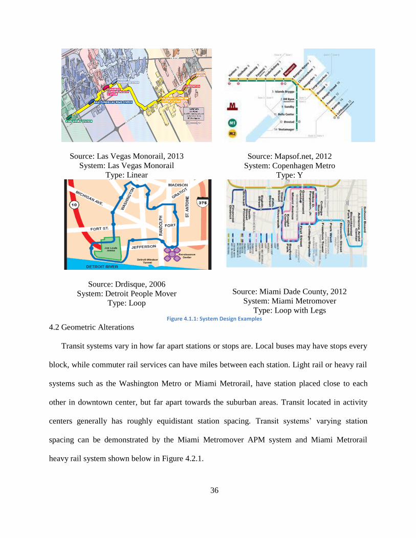
4.1 System Design Types .................................................................................................... 35
4.2 Geometric Alterations ................................................................................................... 36
4.3 Demand Levels ............................................................................................................. 38
4.4 Demand Distribution ..................................................................................................... 40
4.5 Combining Variables .................................................................................................... 41
Chapter 5: Simulation Results ...................................................................................................... 42
5.1 Dual lane ....................................................................................................................... 43
5.2 Y .................................................................................................................................... 45
5.3 Loop .............................................................................................................................. 48
Page 6
iv
5.4 Loop with Legs ............................................................................................................. 50
5.5 Overall........................................................................................................................... 54
Chapter 6: Application .................................................................................................................. 55
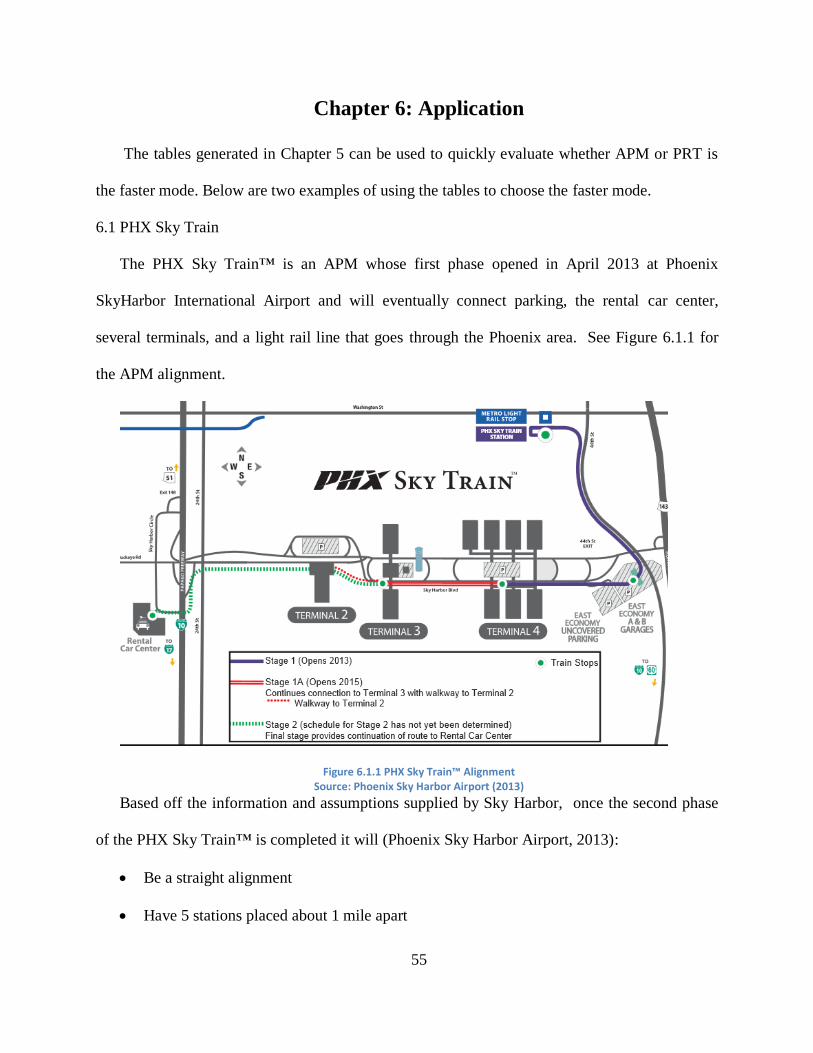
6.1 PHX Sky Train .............................................................................................................. 55
6.2 Detroit People Mover .................................................................................................... 56
Chapter 7: Post Simulation Analyses ............................................................................................ 57
7.1 Velocity ......................................................................................................................... 57
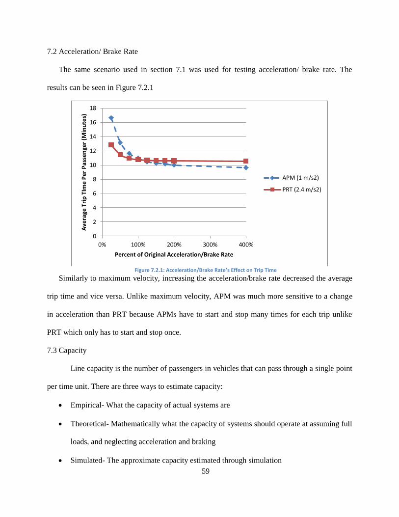
7.2 Acceleration/ Brake Rate .............................................................................................. 59
7.3 Capacity ........................................................................................................................ 59
7.4 Sensitivity of Travel Time to Demand.......................................................................... 60
Chapter 8: Conclusions ................................................................................................................. 63
Appendix 1: Sample APMSM Code ............................................................................................. 65
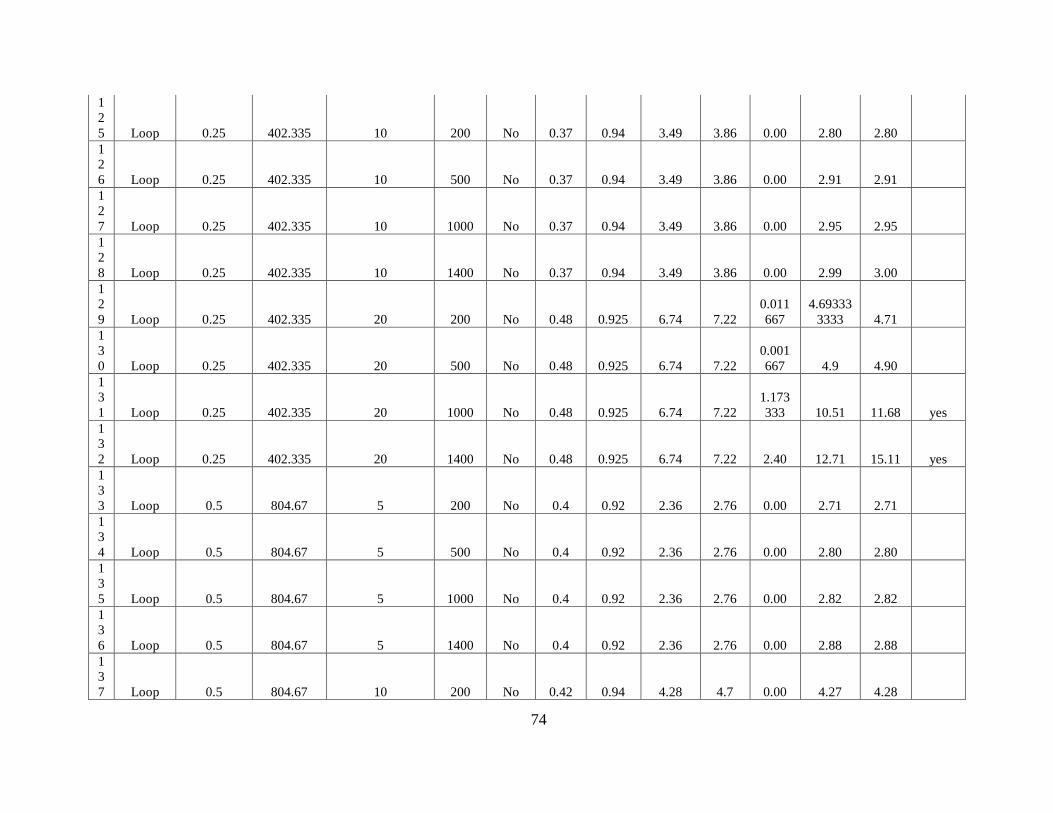
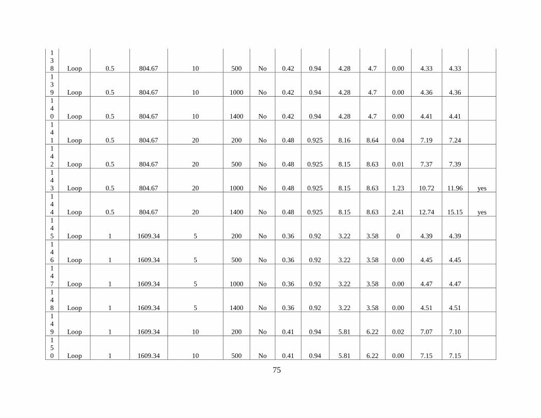
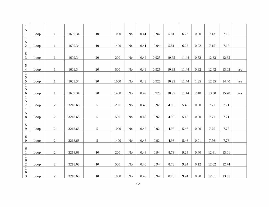
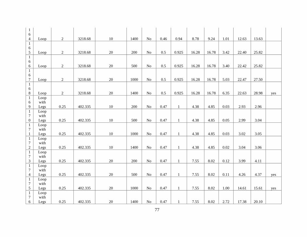
Appendix 2: Scenarios .................................................................................................................. 67
References ..................................................................................................................................... 81
Page 7
v
List of Tables
Table 2.3.1: Purple Line Trip Time Comparison .......................................................................... 19
Table 2.3.2: Purple Line Cost Comparison ................................................................................... 19
Table 4.3.1 Transit System’s Daily Boardings per Station ........................................................... 39
Table 4.3.2: Scenario Demand Levels .......................................................................................... 40
Table 4.4.1: Washington Metro Median Outer Suburban Core Origin Destination Combination 40
Table 5.1.1 Dual Lane Graph Matrix ............................................................................................ 43
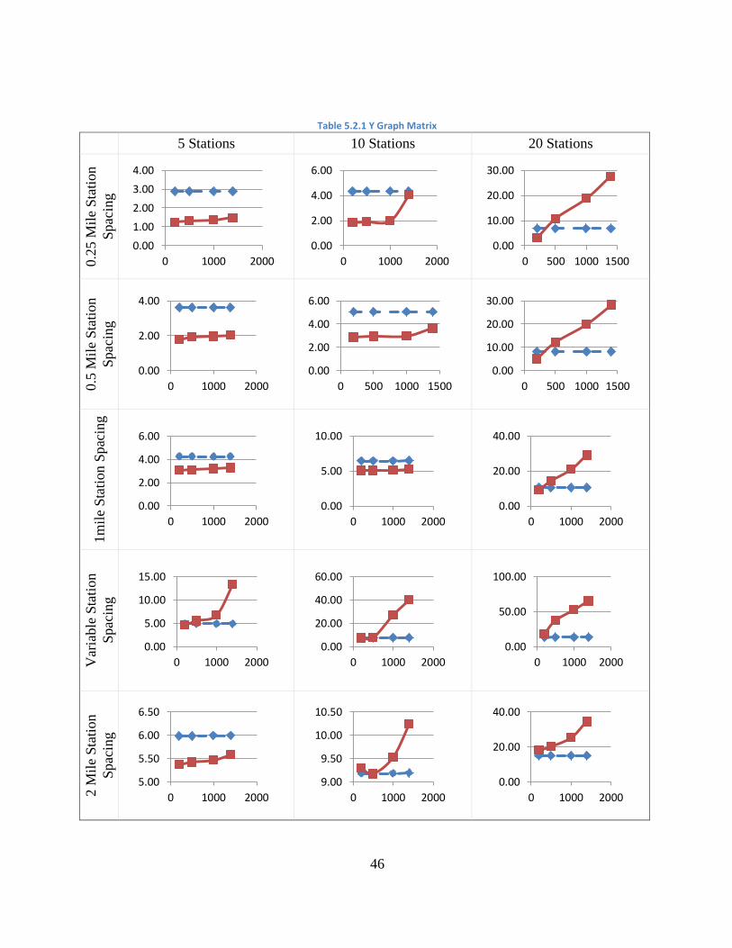
Table 5.2.1 Y Graph Matrix .......................................................................................................... 46
Table 5.3.1: Loop Graph Matrix ................................................................................................... 49
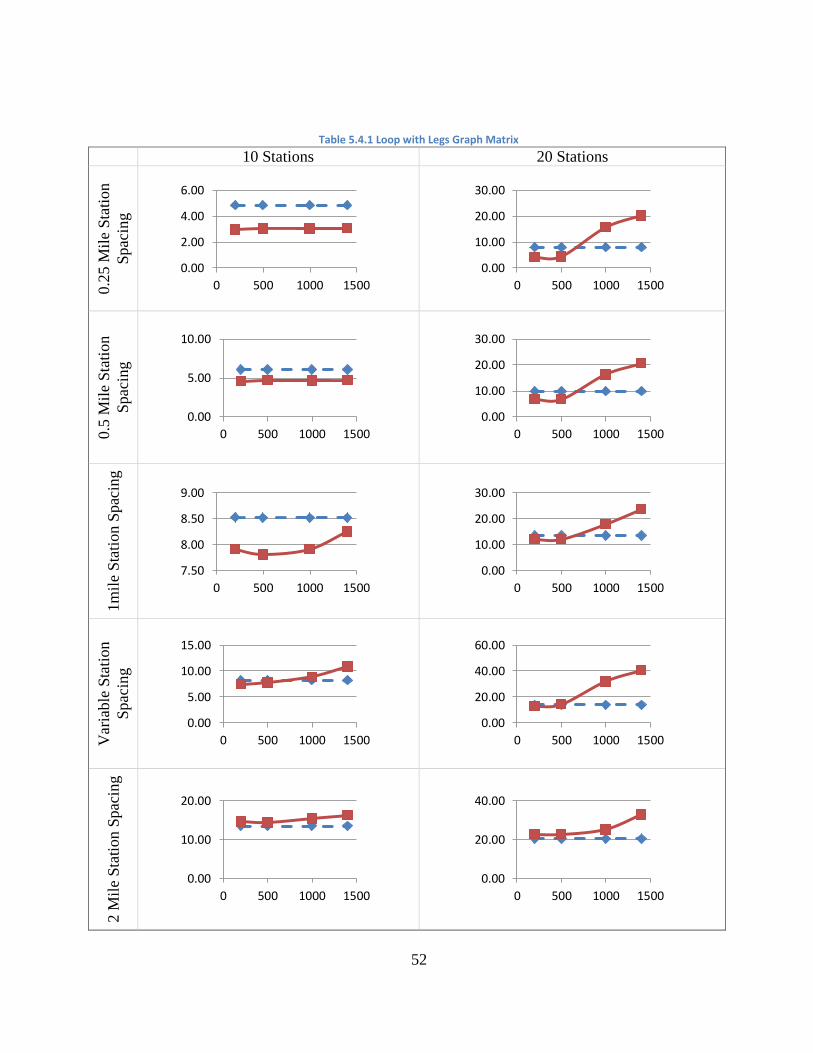
Table 5.4.1 Loop with Legs Graph Matrix ................................................................................... 52
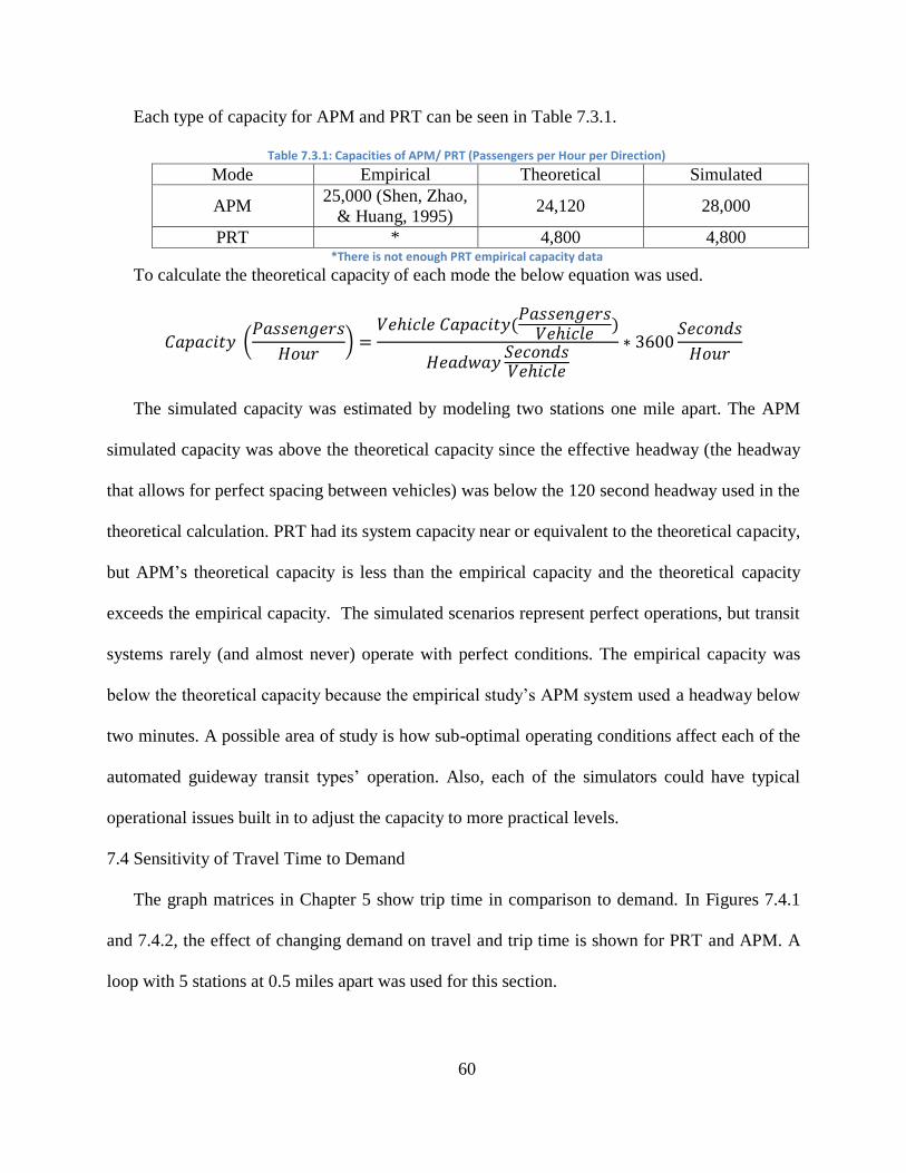
Table 7.3.1: Capacities of APM/ PRT (Passengers per Hour per Direction) ............................... 60
Page 8
vi
List of Figures
Figure 1.1.1: Automated People Mover Types ............................................................................... 2
Figure 1.2.1: Ithaca PRT Network .................................................................................................. 5
Figure 2.1.1: Intra-Airport Mode Comparisons ............................................................................ 12
Figure 2.2.1: Directional Imbalance Example .............................................................................. 13
Figure 2.2.2: Five Berth Serial Type Station ................................................................................ 15
Figure 2.2.3: Four Berth Sawtooth Station w/ Vehicle Entering (Left) and Exiting (Right) Berths
....................................................................................................................................................... 15
Figure 2.2.4: Average Travel Time Sensitivity to Model Variables............................................. 16
Figure 2.2.5: Model Variables’ Effect on Wait Time ................................................................... 17
Figure 2.3.1: LRT/APM Compared to PRT.................................................................................. 18
Figure 3.1.1 APMSM Hierarchy ................................................................................................... 21
Figure 3.1.2: APMSM Networkvisual of Airtrain JFK ................................................................ 22
Figure 3.1.3: Official Airtrain JFK Map ....................................................................................... 23
Figure 3.1.4: Train Movement Rules ............................................................................................ 25
Figure 3.1.5: Additional Dwell Rules for Run Sequence ............................................................. 26
Figure 3.2.1: BeamEd Screenshot ................................................................................................. 29
Figure 3.2.2: Sample Result Display ............................................................................................ 32
Figure 4.1.1: System Design Examples ........................................................................................ 36
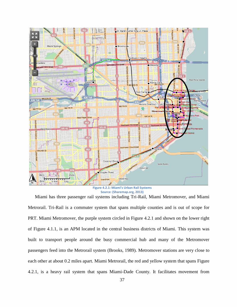
Figure 4.2.1: Miami’s Urban Rail Systems .................................................................................. 37
Figure 5.0.1: Results Graph Example ........................................................................................... 42
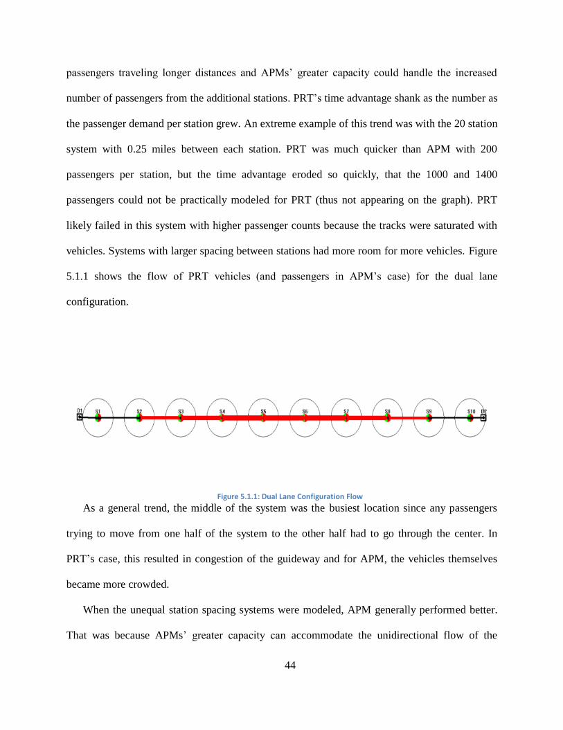
Figure 5.1.1: Dual Lane Configuration Flow................................................................................ 44
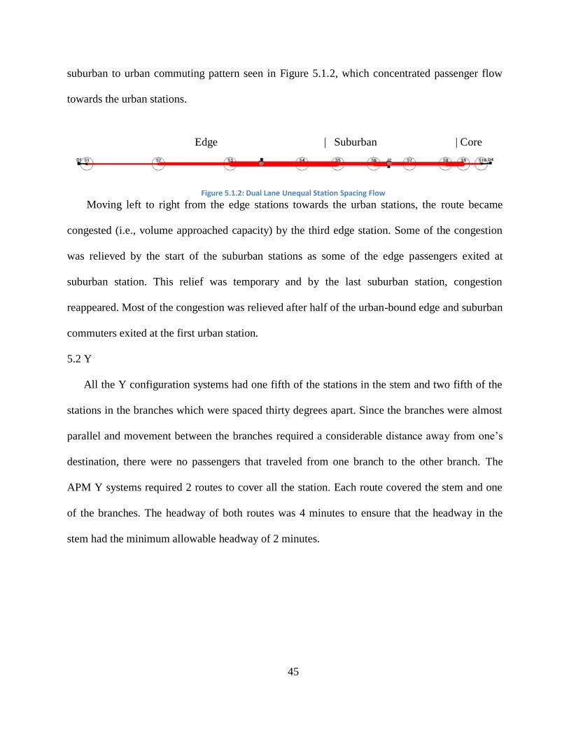
Figure 5.1.2: Dual Lane Unequal Station Spacing Flow .............................................................. 45
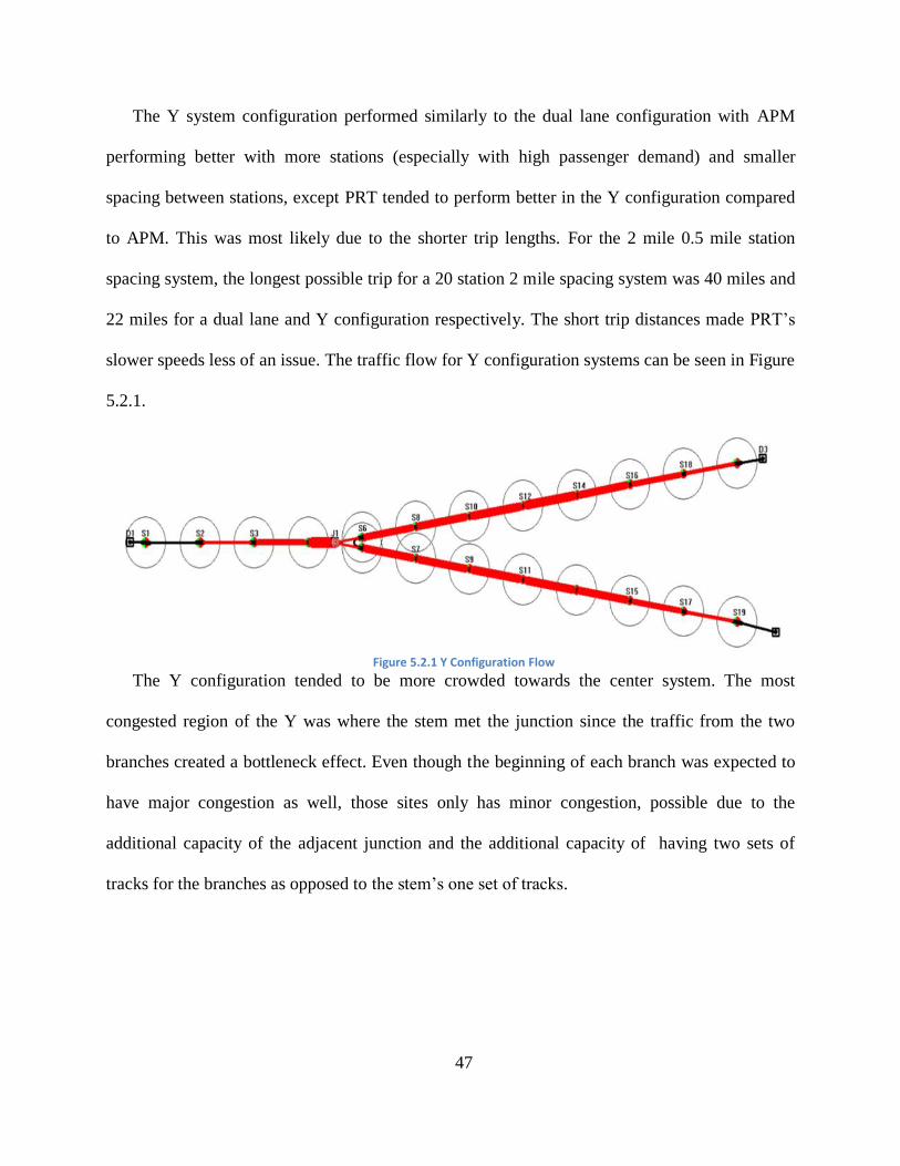
Figure 5.2.1 Y Configuration Flow............................................................................................... 47
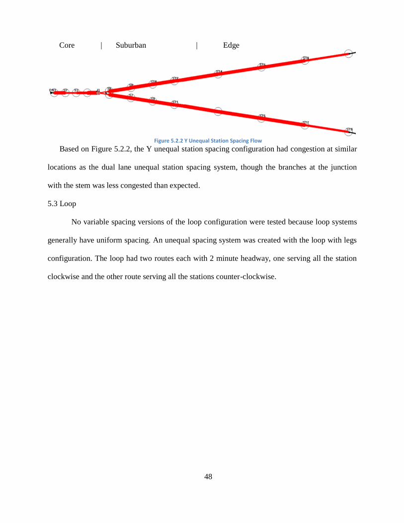
Figure 5.2.2 Y Unequal Station Spacing Flow ............................................................................. 48
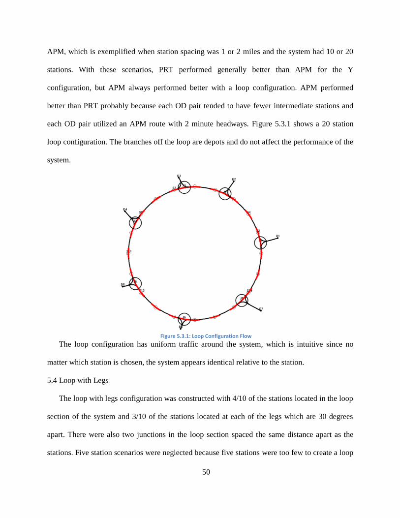
Figure 5.3.1: Loop Configuration Flow ........................................................................................ 50
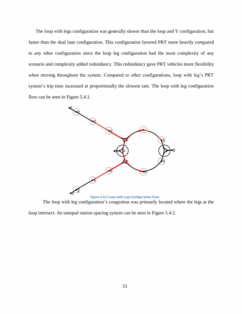
Figure 5.4.1 Loop with Legs Configuration Flow ........................................................................ 53
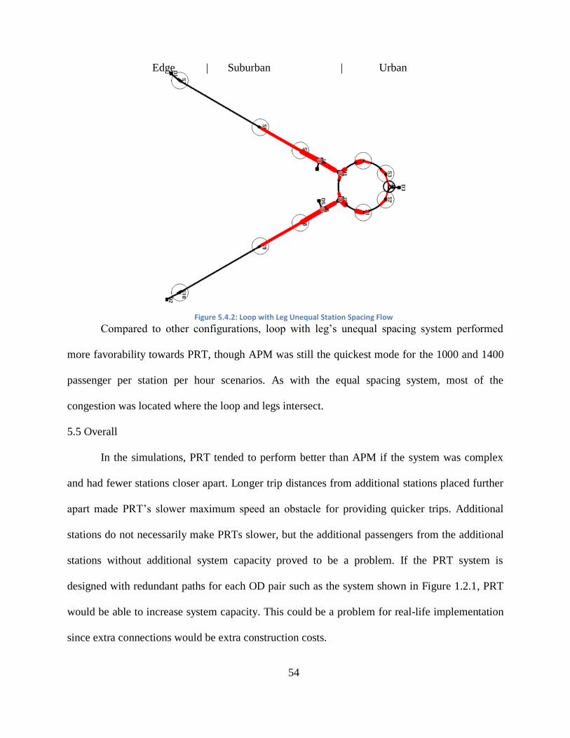
Figure 5.4.2: Loop with Leg Unequal Station Spacing Flow ....................................................... 54
Figure 6.1.1 PHX Sky Train™ Alignment ................................................................................... 55
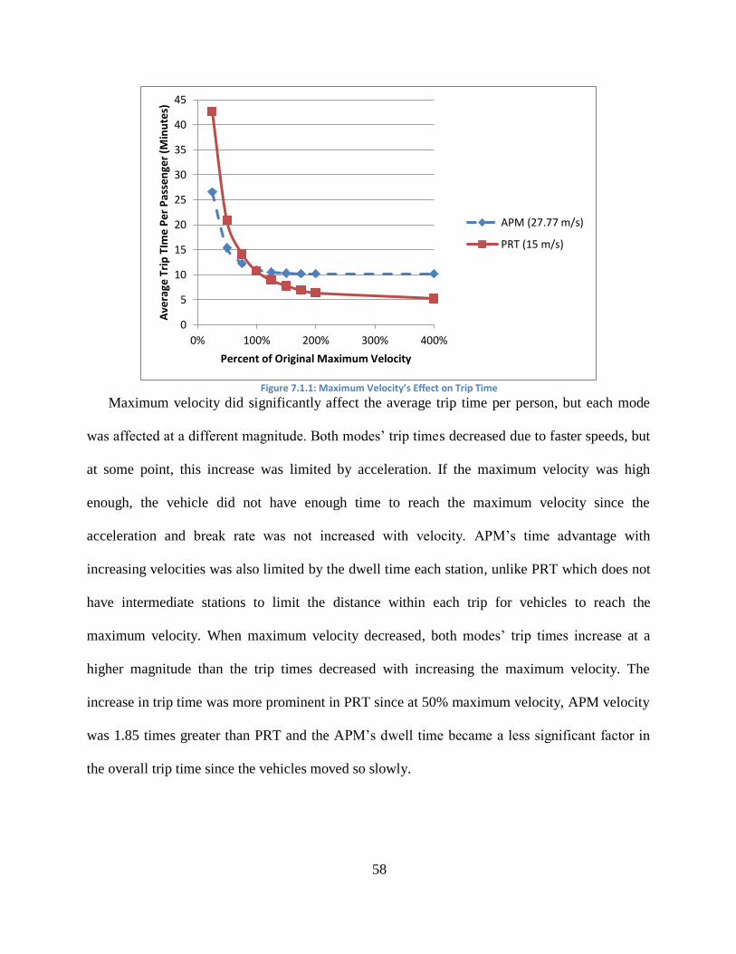
Figure 7.1.1: Maximum Velocity’s Effect on Trip Time.............................................................. 58
Figure 7.2.1: Acceleration/Brake Rate’s Effect on Trip Time...................................................... 59
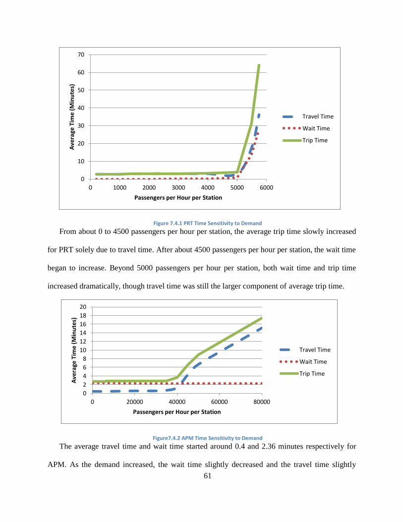
Figure 7.4.1 PRT Time Sensitivity to Demand............................................................................. 61
Figure7.4.2 APM Time Sensitivity to Demand ............................................................................ 61
Page 9
1
Chapter 1: Introduction
Automated fixed-guideway transit includes any type of transit that is completely driverless
and whose motion is constrained by a guideway/ rail. There are two types of automated fixed-
guideway transit that are currently being designed and constructed, namely automated people
movers (APM), and personal rapid transit (PRT).
1.1 APM Background
The Airport Cooperative Research Program’s (ACRP) Report 37, “Guidebook for Planning
and Implementing Automated People Mover Systems at Airports”, defines APMs as “systems
[that] are fully automated and driverless transit systems that operate on fixed guideways in
exclusive rights of way” (ACRP, 2010). Most people associate automated people movers with
the traditional type of APM, which consist of train-like vehicles that move on rubber tires and
powered via an electrified rail or propelled with a cable, but APMs include a family of different
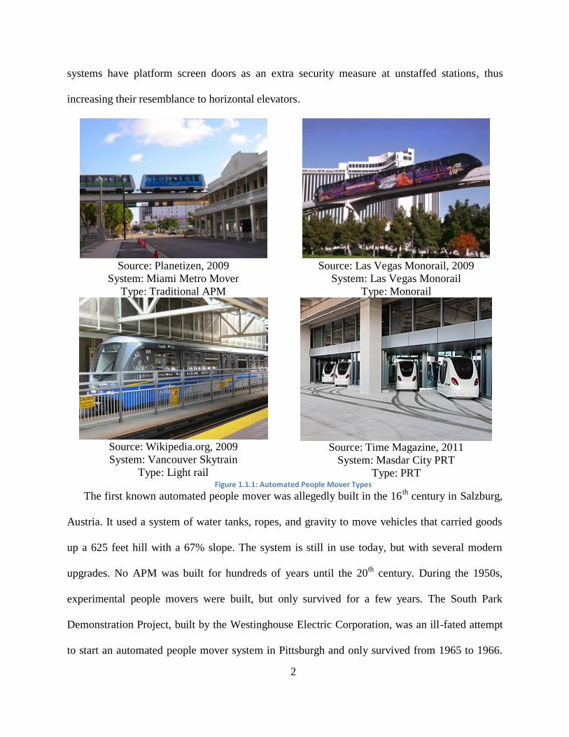
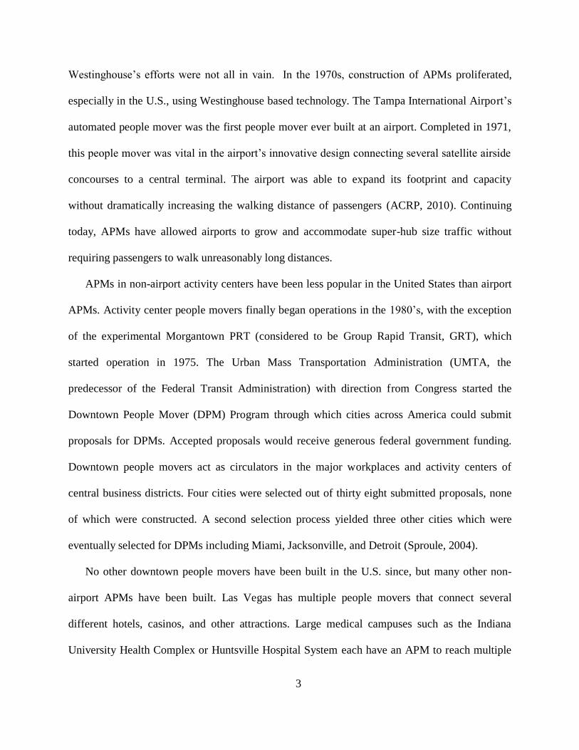
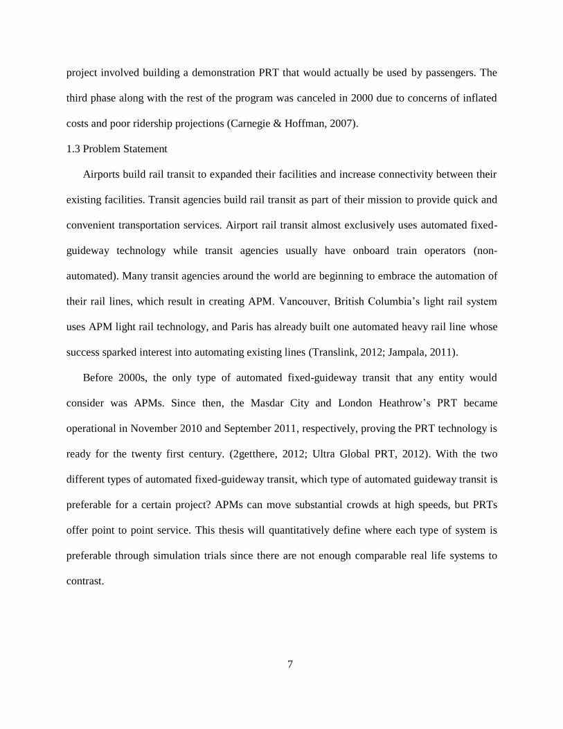
vehicles that are almost as diverse as automobiles (Lewalski, 1997). Figure 1.1.1 shows some
APM examples. Monorail systems vary in shape and size, but all vehicles run above or are
suspended below a single rail or beam (Moore & Little, 1997). Automated light rail and heavy
rail resemble their non-automated counterparts, except that they are fully driverless. Those types
of systems have a large capacity that can handle the travel demands of a busy activity center.
Heavy rail transit systems feature fast trains with many high capacity cars that operate on a fully
grade separate route. Light rail systems are similar, but vehicles tend to be shorter, can be
articulated, and slower than heavy rail (Metro Cincinnati, 2010). The main difference between
heavy and light rail systems are that the latter are designed to run on various types of right-of-
ways, ranging from tracks in mixed traffic to completely exclusive ones. Many of the APM
Page 10
2
systems have platform screen doors as an extra security measure at unstaffed stations, thus
increasing their resemblance to horizontal elevators.
Source: Planetizen, 2009
System: Miami Metro Mover
Type: Traditional APM
Source: Las Vegas Monorail, 2009
System: Las Vegas Monorail
Type: Monorail
Source: Wikipedia.org, 2009
System: Vancouver Skytrain
Type: Light rail
Source: Time Magazine, 2011
System: Masdar City PRT
Type: PRT Figure 1.1.1: Automated People Mover Types
The first known automated people mover was allegedly built in the 16th
century in Salzburg,
Austria. It used a system of water tanks, ropes, and gravity to move vehicles that carried goods
up a 625 feet hill with a 67% slope. The system is still in use today, but with several modern
upgrades. No APM was built for hundreds of years until the 20th
century. During the 1950s,
experimental people movers were built, but only survived for a few years. The South Park
Demonstration Project, built by the Westinghouse Electric Corporation, was an ill-fated attempt
to start an automated people mover system in Pittsburgh and only survived from 1965 to 1966.
Page 11
3
Westinghouse’s efforts were not all in vain. In the 1970s, construction of APMs proliferated,
especially in the U.S., using Westinghouse based technology. The Tampa International Airport’s
automated people mover was the first people mover ever built at an airport. Completed in 1971,
this people mover was vital in the airport’s innovative design connecting several satellite airside
concourses to a central terminal. The airport was able to expand its footprint and capacity
without dramatically increasing the walking distance of passengers (ACRP, 2010). Continuing
today, APMs have allowed airports to grow and accommodate super-hub size traffic without
requiring passengers to walk unreasonably long distances.
APMs in non-airport activity centers have been less popular in the United States than airport
APMs. Activity center people movers finally began operations in the 1980’s, with the exception
of the experimental Morgantown PRT (considered to be Group Rapid Transit, GRT), which
started operation in 1975. The Urban Mass Transportation Administration (UMTA, the
predecessor of the Federal Transit Administration) with direction from Congress started the
Downtown People Mover (DPM) Program through which cities across America could submit
proposals for DPMs. Accepted proposals would receive generous federal government funding.
Downtown people movers act as circulators in the major workplaces and activity centers of
central business districts. Four cities were selected out of thirty eight submitted proposals, none
of which were constructed. A second selection process yielded three other cities which were
eventually selected for DPMs including Miami, Jacksonville, and Detroit (Sproule, 2004).
No other downtown people movers have been built in the U.S. since, but many other non-
airport APMs have been built. Las Vegas has multiple people movers that connect several
different hotels, casinos, and other attractions. Large medical campuses such as the Indiana
University Health Complex or Huntsville Hospital System each have an APM to reach multiple
Page 12
4
hospitals. The Las Colinas Personal Transit System (APM) circulates people around a planned
suburban community. In other countries, APMs have taken on the role of rapid transit,
resembling light rail or high capacity heavy rail. Skytrain provides Vancouver, Canada with
metro capacity and speed without any train operators since the 1980s.
1.2 PRT Background
PRT is another type of automated fixed-guideway transit that utilizes smaller vehicles than
traditional APMs, but provides passengers with direct transportation from origin to destination.
PRT is a type of APM, but in this thesis, APM refers to the traditional type of automated people
movers. PRT enables direct transportation with off-line stations that contain a set of tracks for
vehicles to decelerate and dwell at stations, and another set of tracks to bypass stations at full
speed. PRT networks can be built with complex geometries that cover an entire town without
needing multiple routes as an APM would need. The few PRT systems that exist use multiple
four person unpaired vehicles that are battery powered, but vehicles can fit six people or be
powered by an electrified rail (The Times of India, 2011; Taxi 2000).
PRT is a relatively new mode of transportation that combines features of APMs and taxis.
PRT combine the grade separation and automation of APMs with the capacity and direct origin
to destination transportation capability of taxis. PRT vehicles are not impeded by other PRT
vehicles stopped ahead at stations since PRT stations have their own off-line tracks. Since PRT
vehicles travel directly from origin to destination and stations are separated from the main travel
guideway, PRT is not restricted to simple linear networks (Vectus, 2009). The greatest potential
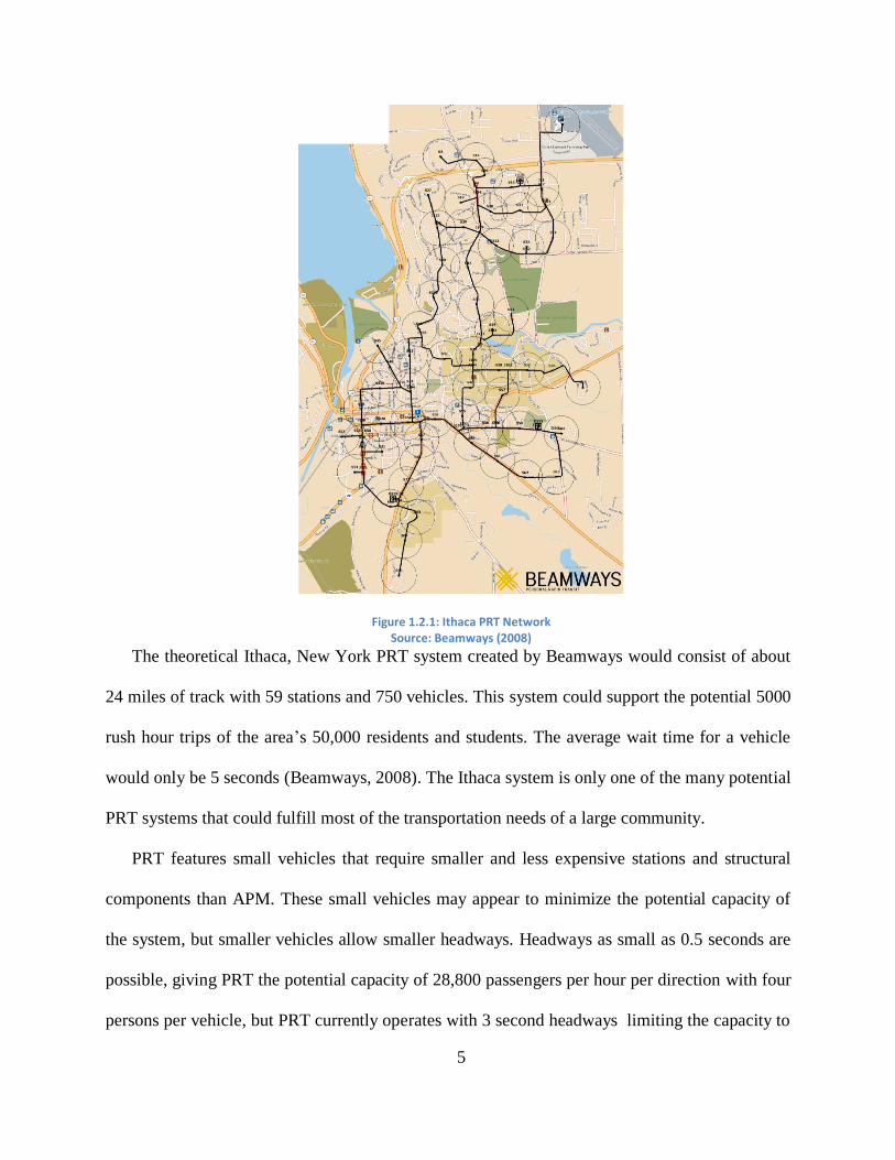
for PRT is with dense networks that cover an entire town as shown in Figure 1.2.1.
Page 13
5
Figure 1.2.1: Ithaca PRT Network Source: Beamways (2008)
The theoretical Ithaca, New York PRT system created by Beamways would consist of about
24 miles of track with 59 stations and 750 vehicles. This system could support the potential 5000
rush hour trips of the area’s 50,000 residents and students. The average wait time for a vehicle
would only be 5 seconds (Beamways, 2008). The Ithaca system is only one of the many potential
PRT systems that could fulfill most of the transportation needs of a large community.
PRT features small vehicles that require smaller and less expensive stations and structural
components than APM. These small vehicles may appear to minimize the potential capacity of
the system, but smaller vehicles allow smaller headways. Headways as small as 0.5 seconds are
possible, giving PRT the potential capacity of 28,800 passengers per hour per direction with four
persons per vehicle, but PRT currently operates with 3 second headways limiting the capacity to
Page 14
6
4,800 passengers per hour per direction. PRT’s main disadvantage is its vehicle performance,
which is slower than APM, reaching speeds only up to 30 mph and acceleration of around 8.2
ft/sec2 (Vectus, 2009).
The notion of PRT was first conceived around 1953 by Donn Fichter, who wrote specifically
of a PRT like system in his 1964 work titled, “Individualized Automated Transit and the City”.
He thought there should be a transportation mode that could be integrated with urban landscapes
with inexpensive and small guideways as well as have service that could meet the transportation
needs of individual riders. Much of the PRT research was performed independently until the
Urban Mass Transportation Act was enacted in 1964. After Congress approved the act, multiple
federal actions supported the progress of advanced transportation systems including PRT. This
led to the development of the first PRT-like system, the Morgantown PRT in the 1970’s. The
USA was not the only country to research PRT technology, the central governments of many
Western European countries and Japan funded PRT test systems in the late 1960’s and 1970’s.
None of the past PRT research projects led to a marketable product except for the German
Cabintaxi system.
The PRT research in the 1980’s was concentrated on the Advanced Group Rapid Transit
program that led to recommendations, but did not produce any functioning PRT or PRT-like
system. PRT research restarted in 1990 when the Chicago Regional Transportation Authority
(RTA) teamed up with the Raytheon Corporation to build a PRT system in the Chicago area.
Phase one of the project involved selecting which company’s technology would be used for the
study. RTA selected Taxi 2000 based technology. For phase two, a 2,200 foot pilot system was
built with an off-line station and three vehicles. This system ran successfully, and proved that the
technology could handle 2.5 second headways. The third and unfortunately last phase of the
Page 15
7
project involved building a demonstration PRT that would actually be used by passengers. The
third phase along with the rest of the program was canceled in 2000 due to concerns of inflated
costs and poor ridership projections (Carnegie & Hoffman, 2007).
1.3 Problem Statement
Airports build rail transit to expanded their facilities and increase connectivity between their
existing facilities. Transit agencies build rail transit as part of their mission to provide quick and
convenient transportation services. Airport rail transit almost exclusively uses automated fixed-
guideway technology while transit agencies usually have onboard train operators (non-
automated). Many transit agencies around the world are beginning to embrace the automation of
their rail lines, which result in creating APM. Vancouver, British Columbia’s light rail system
uses APM light rail technology, and Paris has already built one automated heavy rail line whose
success sparked interest into automating existing lines (Translink, 2012; Jampala, 2011).
Before 2000s, the only type of automated fixed-guideway transit that any entity would
consider was APMs. Since then, the Masdar City and London Heathrow’s PRT became
operational in November 2010 and September 2011, respectively, proving the PRT technology is
ready for the twenty first century. (2getthere, 2012; Ultra Global PRT, 2012). With the two
different types of automated fixed-guideway transit, which type of automated guideway transit is
preferable for a certain project? APMs can move substantial crowds at high speeds, but PRTs
offer point to point service. This thesis will quantitatively define where each type of system is
preferable through simulation trials since there are not enough comparable real life systems to
contrast.
Page 16
8
1.4 Objective
The objective of the thesis is to enable agencies to choose the right type of automated
guideway transit based on passenger travel and waiting time. Other factors such as construction
costs, operating costs, and environmental impacts are very important factors when deciding
which mode to implement for a transit system, but are difficult to quantify for PRT since there
are only two systems currently operating. The lack of other measures of effectiveness is covered
in Chapter 3. Agencies would be able to input the specifications (geometry and passenger
demand) of their proposed automated guideway transit system to discover which type of system
has lower trip times. Results from this study may also be used to improve the design of future
transit projects.
1.4 Organization
The contents of the rest of this thesis are divided into seven chapters. Chapter 2 provides the
literature review that covers APM/PRT’s modeling, capacity analysis, and a comparison of the
modes. Chapter 3 summarizes the simulation tools used to evaluate APM and PRT. Chapter 4
describes how the simulation scenarios were chosen and constructed. Chapter 5 summarizes the
simulation results. Chapter 6 provides an example on how the scenario summaries may be used
to choose between APM and PRT. Chapter 7 provides a sensitivity analysis that gages how
assumptions made in each mode’s acceleration and velocity values affect the simulation results.
Chapter 7 also covers the different capacities of each mode. Lastly, Chapter 8 concludes this
thesis and elaborates on some additional areas of research.
Page 17
9
Chapter 2: Literature Review
The topic of comparing traditional APMs and PRT is not well researched with only a few
papers available, but there is bountiful literature on APMs and PRT individually. The literature
review for this thesis is divided into three sections: Automated People Movers, Personal Rapid
Transit, and PRT and APM Comparisons.
2.1 Automated People Movers
Most traditional APMs are built as short haul transit in airports or specialized activity centers
such as central business districts or campuses. One of the scenarios modeled in this thesis
includes a long line-haul type system which resembles a typical heavy rail corridor. This type of
system is often implemented as a substitute for a light rail or heavy rail line, transporting
commuters across cities. Shen, Zhao, and Huang (1995) proved that line-haul type APMs are
effective at transporting passengers by reviewing existing line-haul APMs including the
Vancouver Skytrain in Canada, Lille Metro in France, and the Wenshan Line of the Taipei Metro
in Taiwan. The systems ranged in length from 7.2 to 17.9 miles with 12 to 36 stations at the time
the paper’s publication. All systems have since been extended. Shen et al. showed how each line-
haul APM system had the capacity and the operating specifications to compete with other forms
of line-haul transit. The systems operated at relatively high capacities with headways as low as 1
minute and their fleets consisted of trains with a capacity of up to 600 passengers per train. The
maximum capacity along a point was 25,000 passengers per hour per direction. The trains could
reach speeds of up to 56 mph (Shen, Zhao, & Huang, 1995). The capacity was on par with light
rail, but on the low end for heavy rail. The speed was comparable to light rail and a bit slower
than heavy rail (Carnegie & Hoffman, 2007). The capital cost figures for each of the APM
systems were highly variable and depended on how much of the alignment was at-grade,
Page 18
10
elevated, or underground. For example, the primarily elevated Skytrain cost about $98.6 million
per mile, while the mostly underground Lille Metro cost about $164.6 million per mile. In
comparison, the average cost per mile for light rail and heavy rail at the time of the study and
adjusted to 2012 dollars was $105.8 and $240.7 million per mile, respectively. In the US and
other developed countries, employee costs make up the largest portion of costs, which APMs
minimize through the lack of on-board operators. Each Vancouver Skytrain employee supported
about 630,000 passenger miles compared to 221,000 passenger miles for heavy rail and 76,300
passenger miles for light rail. As line-haul transit systems, APMs have the performance,
capacity, and cost to be considered along with non-automated heavy rail and light rail (Shen,
Zhao, & Huang, 1995).
Lin and Trani (2000) developed a sophisticated APM simulation model using the specialized
simulation software EXTENDS. Their simulator, APMSIM, was capable of modeling
passenger/vehicle movement, system performance, and energy consumption based on a number
of input blocks. Besides the simulation specifics and station component blocks, there were a
number of guideway blocks that included two-way switches, merge diverge, single-lane loop,
pinched loop, turnaround, and single lane blocks. The simulation user would assemble the blocks
together to create an APM model. The user specified through blocks the passengers’ origin
destination pattern, network geometry, and demand over time. The simulation assumed:
Passengers first exit vehicles before new passengers enter
Boarding time per passenger was deterministic (though it was possible to use a
distribution)
Acceleration was based on equations of motion
The braking rate was constant
Page 19
11
Lin and Trani used APMSIM to model Atlanta Hartsfield International Airport’s Plane Train.
For that particular example they assumed that:
Each vehicle had two doors that took 1.5 seconds to open/close and took 1 sec for a
passenger to enter/exit each door
Braking rate was 1 m/sec2
Station dwell time was 35 seconds
Headway between trains must be a minimum of 120 seconds apart
The simulation successfully allowed them to model energy consumption, waiting time,
queues at stations, and many other variables of interest (Lin & Trani, 2000).
ACRP 37, “Guidebook for Planning and Implementing Automated People Mover Systems at
Airports”, provided a variety of information on APMs. One of the most important issues was
what instances should an APM be considered at all. If a trip is short enough, the station access
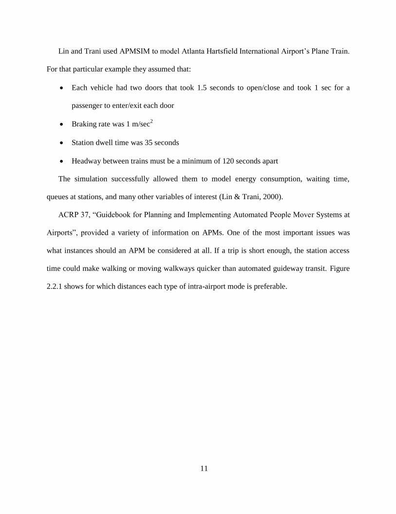
time could make walking or moving walkways quicker than automated guideway transit. Figure
2.2.1 shows for which distances each type of intra-airport mode is preferable.
Page 20
12
Figure 2.1.1: Intra-Airport Mode Comparisons
Source: ACRP (2010)
For trips under 300 feet, walking or moving walkways was the fastest. The travel time
savings for APMs really started to pay off after about 800 feet when the dwell time and stopping
sequences had less of an effect on the overall trip time.
ACRP 37 also had recommendations on the design and operation of the system. When
designing an APM’s alignment, ACRP 37 recommended curve radii greater than 300 feet (91.5
meter) and a bare minimum radius of 150 feet (45.72 meter) which drastically impacted
allowable speed. Minimum allowable headway between trains was recommended as 1.5 minutes.
Maximum speeds varied for each vehicle type, but were typically 32 to 40 mph (ACRP, 2010).
2.2 Personal Rapid Transit
Gluck and Anspach (1997) used PRT2000 NETSIM, a PRT simulator, to run various
sensitivity analyzes on PRTs. In the first analysis, average trip length and trip speed was shifted
in a system with 100 vehicles to yield how many vehicle trips per hour the PRT can produce.
Page 21
13
The simulations showed that the higher the average trip speed and lower the average trip length,
the more trips per hour the system was able to supply. Increasing trip speed from 20 to 30 mph
increased the capacity of the system by about 50%. Doubling the average trip length halved the
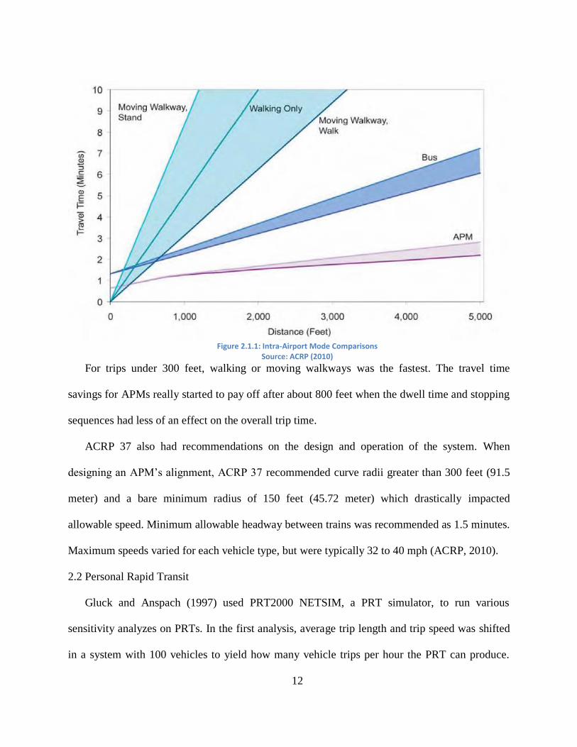
capacity. During certain periods of time, especially rush hours, trips tend to go mainly in one
direction and with PRTs, empty vehicles must run against the direction of travel to make up for
the “unbalanced” demand. Gluckand Anspach showed that the capacity of a system decreased as
its demand became more directionally unbalanced. For example, the transit route in Figure 2.2.1
was 100% directionally balanced between 0 and 0.5, and 0% balanced between 0.5 and 1. Even
though the sum of passengers in both directions stayed constant throughout the route, the region
between 0.5 and 1 was on the verge of being overloaded since all the passengers rode the route in
one direction. Lastly, with lower travel speeds, the system could accommodate more vehicles,
though not necessarily more trips (Gluck & Anspach, 1997).
Figure 2.2.1: Directional Imbalance Example
Gluck and Anspach (1997) looked at how different travel characteristics could affect the
capacity of the PRT system, but what about the capacity of the PRT stations themselves?
Schweizer, Mantecchini, and Greenwood (2011) specially studied the capacity of the PRT
Pas
senger
s per
Hour
Page 22
14
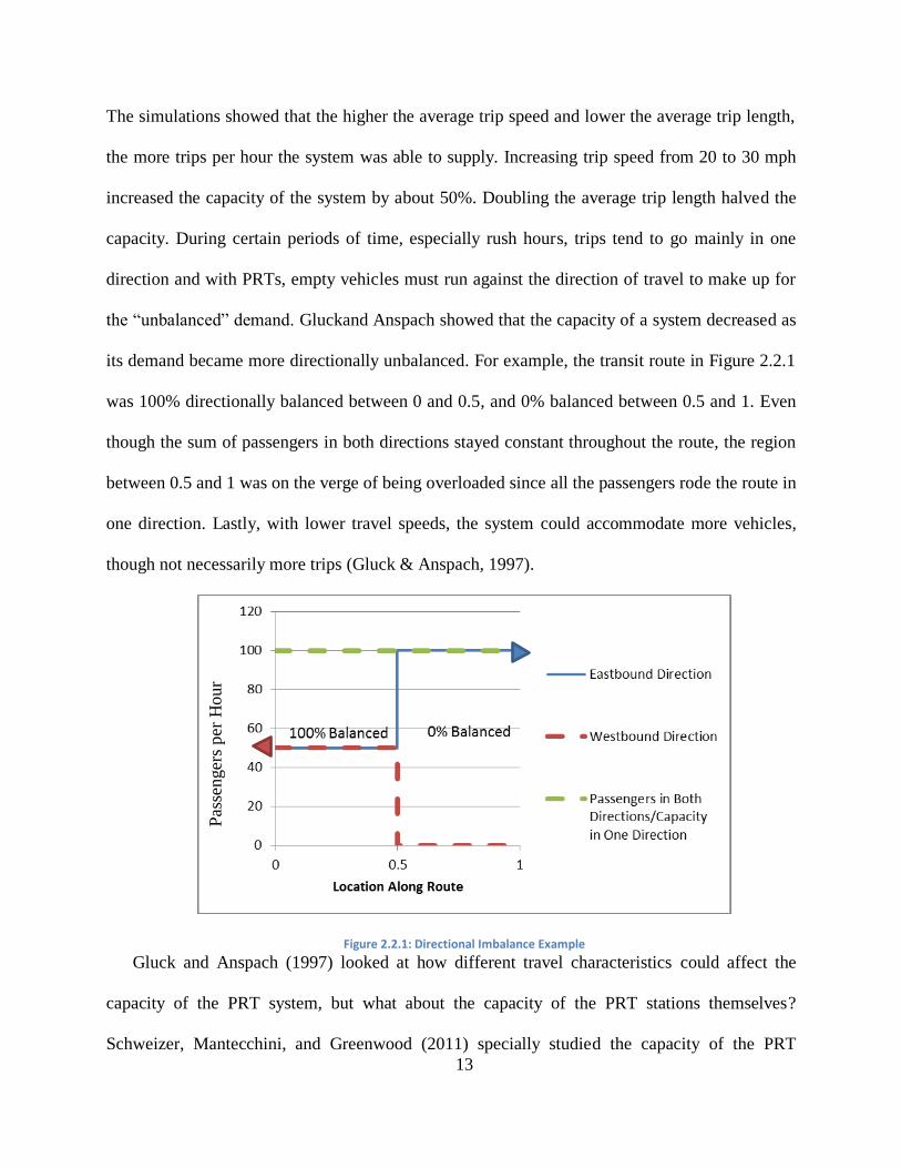
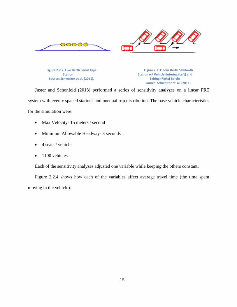
stations. The capacity of the two main types of PRT stations, serial off-line (figure 2.2.2) and
sawtooth (figure 2.2.3) stations was examined. Serial type stations typically have a single
platform where vehicles queue up to accept passengers. The first vehicle to enter is the first
vehicle exit the station. The serial type station had the best capacity, theoretically able to handle
almost 800 vehicles per hour assuming the stations had 12 berths and each vehicle was loaded
with four passengers with heavy luggage. 12 berth stations had the capacity for over 1000
vehicles per hour if there was only one passenger without baggage per vehicle. The major flaw
for this station type was that loading a slow passenger will slow down the entire station
(Schweizer, Mantecchini, & Greenwood, 2011).
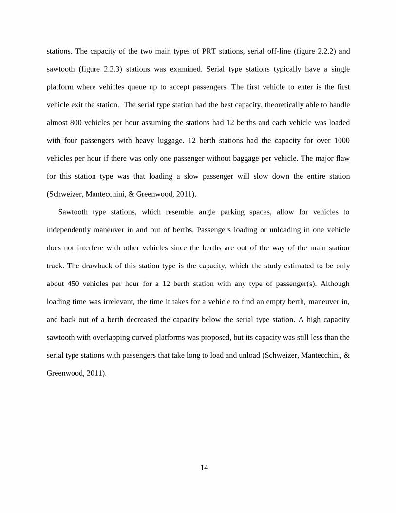
Sawtooth type stations, which resemble angle parking spaces, allow for vehicles to
independently maneuver in and out of berths. Passengers loading or unloading in one vehicle
does not interfere with other vehicles since the berths are out of the way of the main station
track. The drawback of this station type is the capacity, which the study estimated to be only
about 450 vehicles per hour for a 12 berth station with any type of passenger(s). Although
loading time was irrelevant, the time it takes for a vehicle to find an empty berth, maneuver in,
and back out of a berth decreased the capacity below the serial type station. A high capacity
sawtooth with overlapping curved platforms was proposed, but its capacity was still less than the
serial type stations with passengers that take long to load and unload (Schweizer, Mantecchini, &
Greenwood, 2011).
Page 23
15
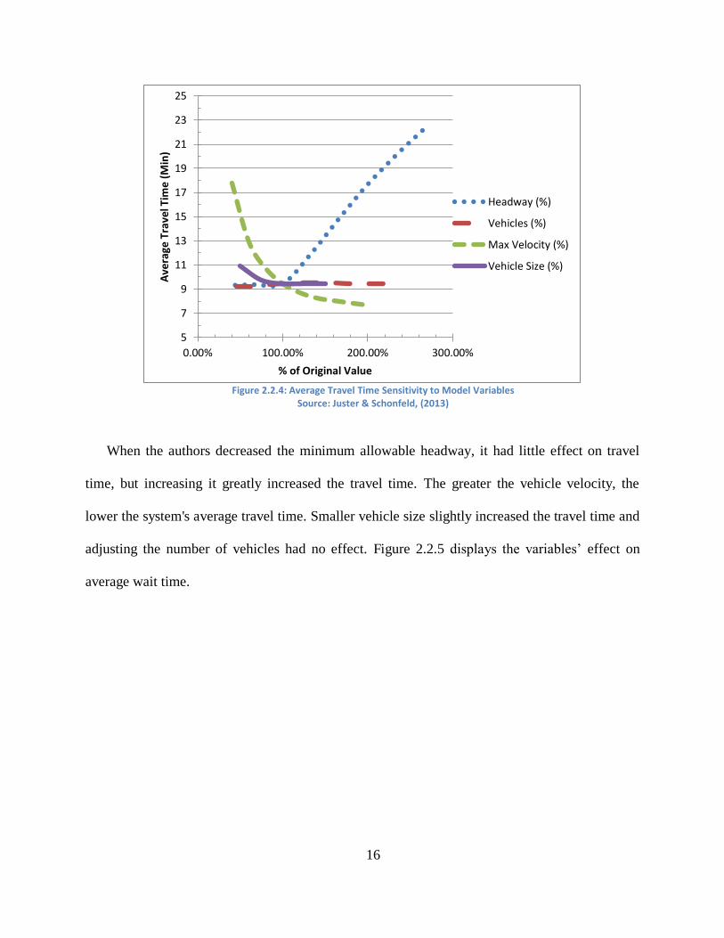
Juster and Schonfeld (2013) performed a series of sensitivity analyzes on a linear PRT
system with evenly spaced stations and unequal trip distribution. The base vehicle characteristics
for the simulation were:
Max Velocity- 15 meters / second
Minimum Allowable Headway- 3 seconds
4 seats / vehicle
1100 vehicles
Each of the sensitivity analyzes adjusted one variable while keeping the others constant.
Figure 2.2.4 shows how each of the variables affect average travel time (the time spent
moving in the vehicle).
Figure 2.2.2: Five Berth Serial Type Station
Source: Schweizer et al. (2011).
Figure 2.2.3: Four Berth Sawtooth Station w/ Vehicle Entering (Left) and
Exiting (Right) Berths Source: Schweizer et al. (2011).
Page 24
16
Figure 2.2.4: Average Travel Time Sensitivity to Model Variables
Source: Juster & Schonfeld, (2013)
When the authors decreased the minimum allowable headway, it had little effect on travel
time, but increasing it greatly increased the travel time. The greater the vehicle velocity, the
lower the system's average travel time. Smaller vehicle size slightly increased the travel time and
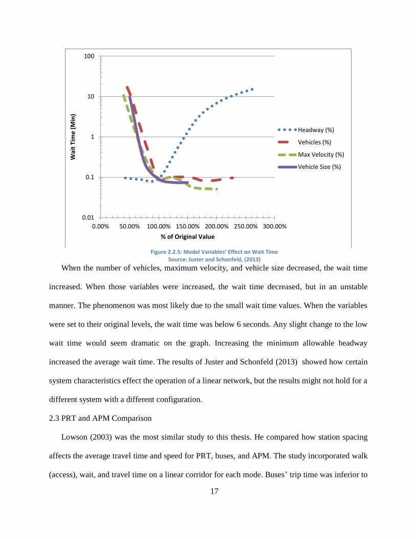
adjusting the number of vehicles had no effect. Figure 2.2.5 displays the variables’ effect on
average wait time.
5
7
9
11
13
15
17
19
21
23
25
0.00% 100.00% 200.00% 300.00%
Ave
rage
Tra
vel T
ime
(Min
)
% of Original Value
Headway (%)
Vehicles (%)
Max Velocity (%)
Vehicle Size (%)
Page 25
17
Figure 2.2.5: Model Variables’ Effect on Wait Time
Source: Juster and Schonfeld, (2013)
When the number of vehicles, maximum velocity, and vehicle size decreased, the wait time
increased. When those variables were increased, the wait time decreased, but in an unstable
manner. The phenomenon was most likely due to the small wait time values. When the variables
were set to their original levels, the wait time was below 6 seconds. Any slight change to the low
wait time would seem dramatic on the graph. Increasing the minimum allowable headway
increased the average wait time. The results of Juster and Schonfeld (2013) showed how certain
system characteristics effect the operation of a linear network, but the results might not hold for a
different system with a different configuration.
2.3 PRT and APM Comparison
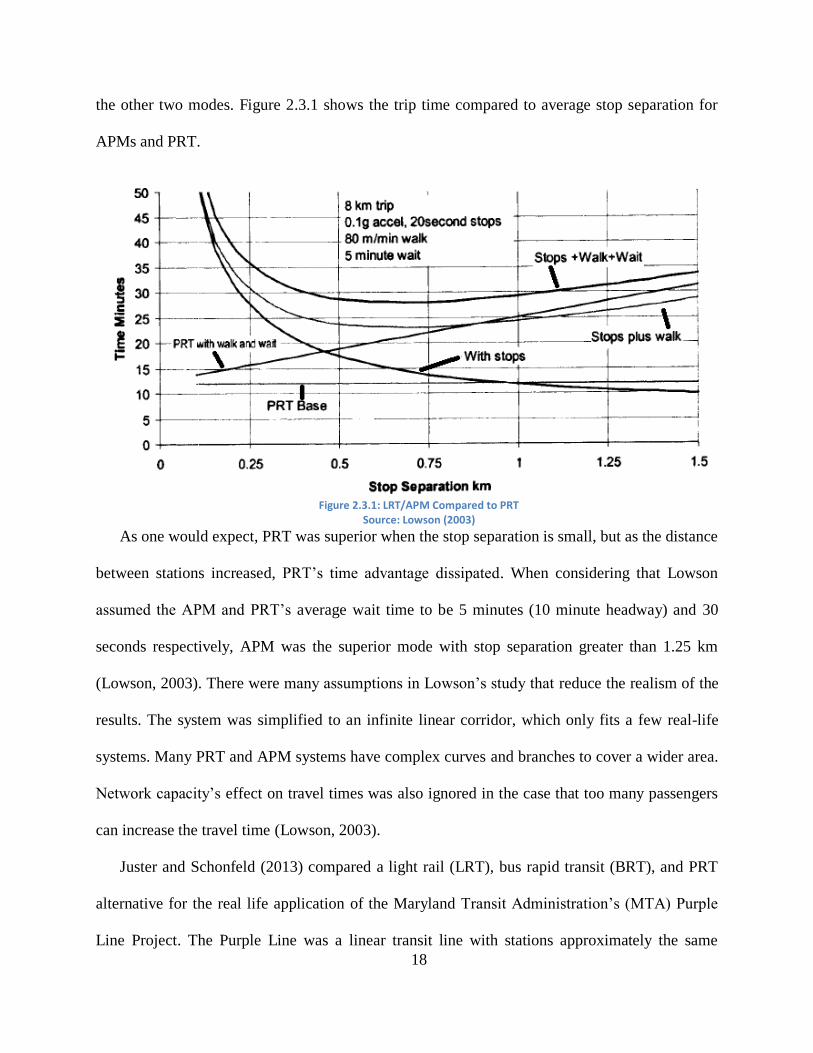
Lowson (2003) was the most similar study to this thesis. He compared how station spacing
affects the average travel time and speed for PRT, buses, and APM. The study incorporated walk
(access), wait, and travel time on a linear corridor for each mode. Buses’ trip time was inferior to
0.01
0.1
1
10
100
0.00% 50.00% 100.00% 150.00% 200.00% 250.00% 300.00%
Wai
t Ti
me
(Min
)
% of Original Value
Headway (%)
Vehicles (%)
Max Velocity (%)
Vehicle Size (%)
Page 26
18
the other two modes. Figure 2.3.1 shows the trip time compared to average stop separation for
APMs and PRT.
Figure 2.3.1: LRT/APM Compared to PRT
Source: Lowson (2003)
As one would expect, PRT was superior when the stop separation is small, but as the distance
between stations increased, PRT’s time advantage dissipated. When considering that Lowson
assumed the APM and PRT’s average wait time to be 5 minutes (10 minute headway) and 30
seconds respectively, APM was the superior mode with stop separation greater than 1.25 km
(Lowson, 2003). There were many assumptions in Lowson’s study that reduce the realism of the
results. The system was simplified to an infinite linear corridor, which only fits a few real-life
systems. Many PRT and APM systems have complex curves and branches to cover a wider area.
Network capacity’s effect on travel times was also ignored in the case that too many passengers
can increase the travel time (Lowson, 2003).
Juster and Schonfeld (2013) compared a light rail (LRT), bus rapid transit (BRT), and PRT
alternative for the real life application of the Maryland Transit Administration’s (MTA) Purple
Line Project. The Purple Line was a linear transit line with stations approximately the same
Page 27
19
distance from each other, but with an uneven trip distribution. Some multimodal stations (i.e.
Purple Line stations with Metrorail, commuter rail, Amtrak, and bus connections) had over 12
times the trip origins and destinations as adjacent unimodal stations. Although the LRT and BRT
alternatives were not APMs, they were transit modes that stop at each station, like traditional
APMs. The paper superimposed a PRT network system on top of the Purple Line’s planned
alignment using the BeamEd PRT simulator, the same program utilized for PRT modeling in this
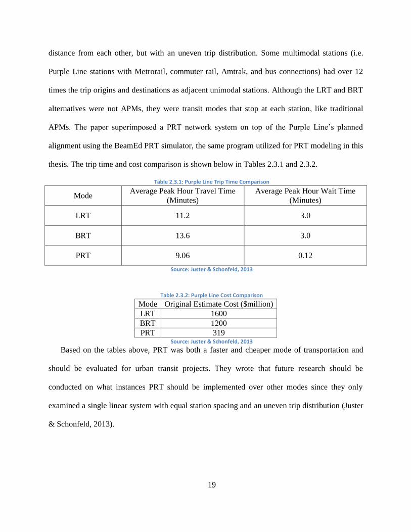
thesis. The trip time and cost comparison is shown below in Tables 2.3.1 and 2.3.2.
Table 2.3.1: Purple Line Trip Time Comparison
Mode Average Peak Hour Travel Time
(Minutes)
Average Peak Hour Wait Time
(Minutes)
LRT 11.2 3.0
BRT 13.6 3.0
PRT 9.06 0.12
Source: Juster & Schonfeld, 2013
Table 2.3.2: Purple Line Cost Comparison
Mode Original Estimate Cost ($million)
LRT 1600
BRT 1200
PRT 319 Source: Juster & Schonfeld, 2013
Based on the tables above, PRT was both a faster and cheaper mode of transportation and
should be evaluated for urban transit projects. They wrote that future research should be
conducted on what instances PRT should be implemented over other modes since they only
examined a single linear system with equal station spacing and an uneven trip distribution (Juster
& Schonfeld, 2013).
Page 28
20
Chapter 3: Methodology
Multiple simulation trials were created for this thesis since there are not enough real life
examples to aggregate and compare. PRT and APM were modeled with their own software
which each has its separate input format, output format, assumptions, and limitations. Even
though each mode used different software, the input for each scenario was identical. The settings
for both PRT and APM are programed to resemble systems with the highest possible capacity,
since the goal of this thesis is to find which type of automated guideway transit can handle which
type of loads for specific geometry, rather than optimizing the number of vehicles. Trip time is
the measure of effectiveness (MOE) in this thesis, though other MOEs such as cost were also
considered.
3.1 APM Simulation Methodology
The APM model, Automated People Mover Simulation Model (APMSM), is a Java based
simulation that runs directly from code without a graphical user interface (GUI). APMSM was
created by the author to estimate APM system performance and energy consumption. APMSM
requires the user to input the system geometry, service routes, train characteristics, and passenger
demand. Once the simulation is running, a set of rules govern vehicle motion and passenger
distribution. The actual operation of an APM is complex, and APMSM makes many assumptions
to best approximate the actual operation without being computationally intensive. Some of the
assumptions include deterministic passenger arrival, two-dimensional operation, and perfect
performance. After the simulation finished, the user has multiple output files available to show
the system performance down to each train and second.
Page 29
21
3.1.1 APMSM Input Requirements
APMSM required a large amount of input to run each simulation. See Figure 3.1.1 for the
APMSM hierarchy.
Figure 3.1.1 APMSM Hierarchy
Each scenario for the thesis needed its own Supernetwork, which contained all the
components needed to create a unique APM. By default, each Supernetwork contained a:
Networkgraph- Contained all the APM track and station components
Routes- Contained different groups of stations and directions
Networktrain- Contained all the trains and the rules that dictate the trains’ movement
Networkpassenger- Contained the passengers and demand levels
Networkvisual- Helped the user visualize the Networkgraph
Each scenario’s Networkgraph started with the creation of stations. Stations consisted of a
name, x coordinate, and y coordinate. The x and y coordinates could be in any unit, but needed to
be consistent with the other units used in the simulation. For this thesis, they were in meters. The
stations were then connected with track sections including one-way and bidirectional tracks. The
Supernetwork
Networkgraph
Stations
Depot
Waypoints
Curves
Networktrain
Trains
Networkpassenger Route
Directions
Networkvisual
Page 30
22
simulation assumed the track sections were straight unless waypoints or curves were created in
the Networkgraph. Waypoints acted as intermediate points between stations. Curves are a series
of waypoints and connections based on the user’s specified radius and number of intermediate
points. Curves and waypoints were essential for creating the complex geometries in this thesis.
Every scenario’s Supernetwork required a depot to store the trains and acted as the trains’
starting location during the simulation. A depot was usually placed at one of the ends of a
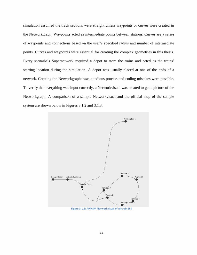
network. Creating the Networkgraphs was a tedious process and coding mistakes were possible.
To verify that everything was input correctly, a Networkvisual was created to get a picture of the
Networkgraph. A comparison of a sample Networkvisual and the official map of the sample
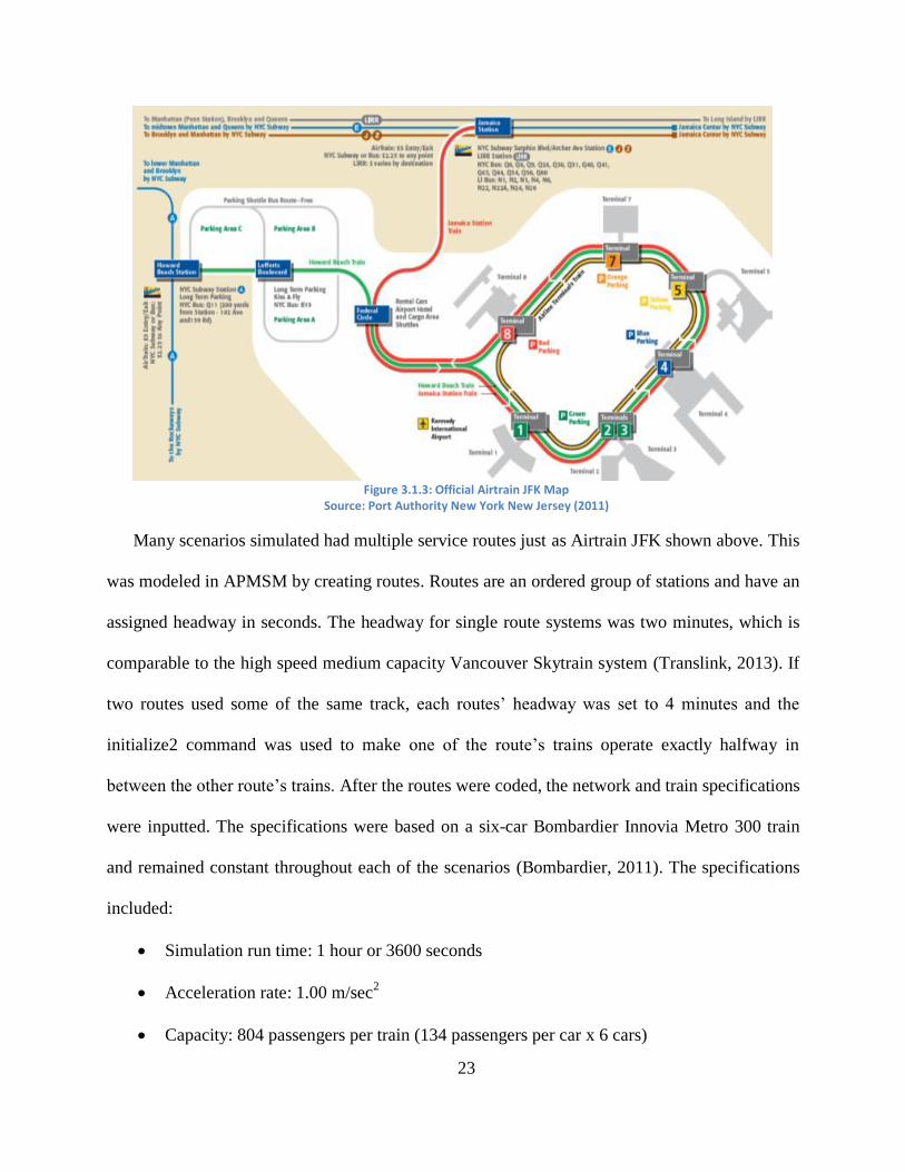
system are shown below in Figures 3.1.2 and 3.1.3.
Figure 3.1.2: APMSM Networkvisual of Airtrain JFK
Page 31
23
Figure 3.1.3: Official Airtrain JFK Map
Source: Port Authority New York New Jersey (2011)
Many scenarios simulated had multiple service routes just as Airtrain JFK shown above. This
was modeled in APMSM by creating routes. Routes are an ordered group of stations and have an
assigned headway in seconds. The headway for single route systems was two minutes, which is
comparable to the high speed medium capacity Vancouver Skytrain system (Translink, 2013). If
two routes used some of the same track, each routes’ headway was set to 4 minutes and the
initialize2 command was used to make one of the route’s trains operate exactly halfway in
between the other route’s trains. After the routes were coded, the network and train specifications
were inputted. The specifications were based on a six-car Bombardier Innovia Metro 300 train
and remained constant throughout each of the scenarios (Bombardier, 2011). The specifications
included:
Simulation run time: 1 hour or 3600 seconds
Acceleration rate: 1.00 m/sec2
Capacity: 804 passengers per train (134 passengers per car x 6 cars)
Page 32
24
Brake rate: 1.00 m/sec2
Dwell time: 35 seconds
Diffusion rate:36 passengers/seconds
Maximum speed: 27.77 m/sec (100 km/hr)
Next, the scenarios were initialized by having the simulation release a single train for each
route one at a time, all while collecting the travel time between each station. The simulation
used this information to calculate how many trains were needed for each of the scenarios’ routes
and which route was the best route for each origin destination (OD) pair. Each route was
assigned a fleet of trains based on the route’s designated headway. The headway was decreased
to an effective headway so when the simulation divided total travel time by the headway to
calculate the fleet size, the resulting number is an integer. OD pairs refer to the set of passengers
going from one origin to a specific destination. If multiple routes covered the same OD pair,
passengers would use the fastest route and any other route which travel time exceeded the
quickest route by below the user specified threshold (1 minute). Finally, the hourly passenger
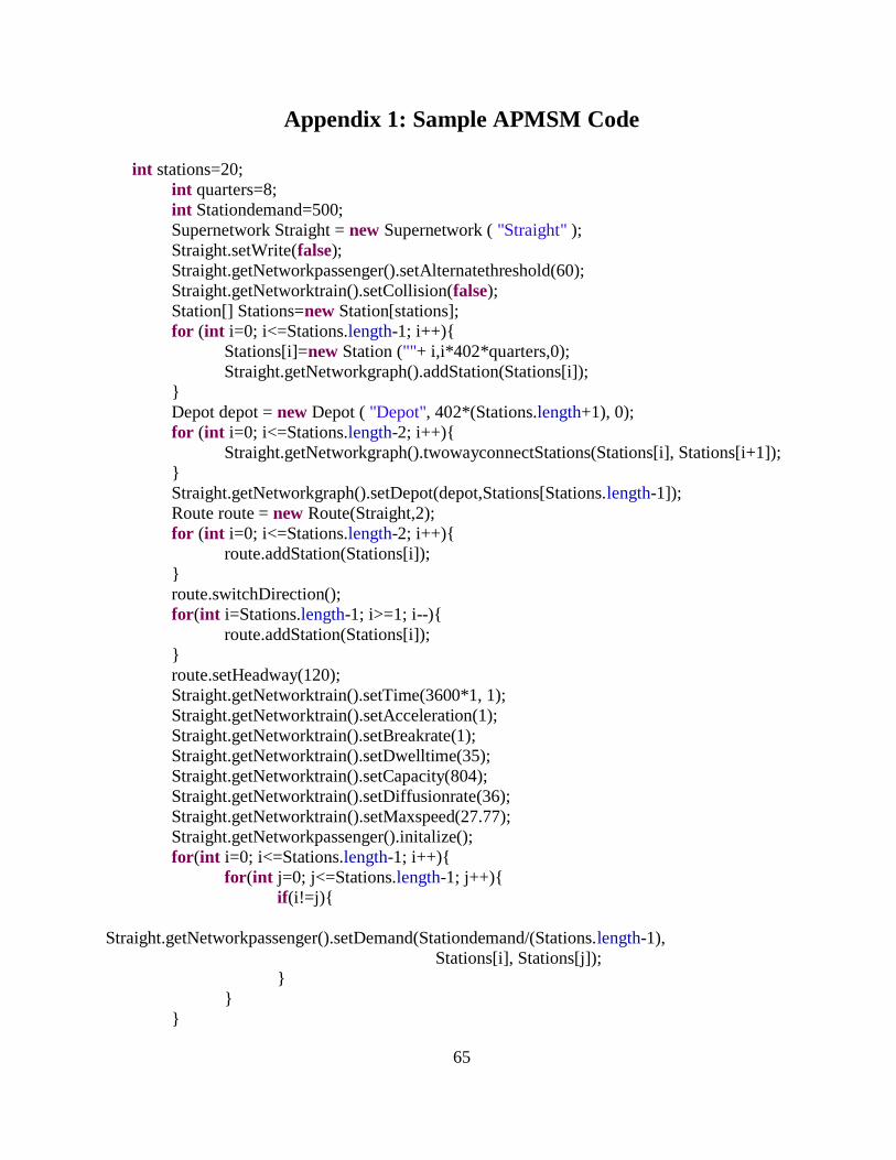
demand for each OD pair was set for each scenario. A sample of the code can be seen in
Appendix 1.
3.1.2 APMSM Mechanics
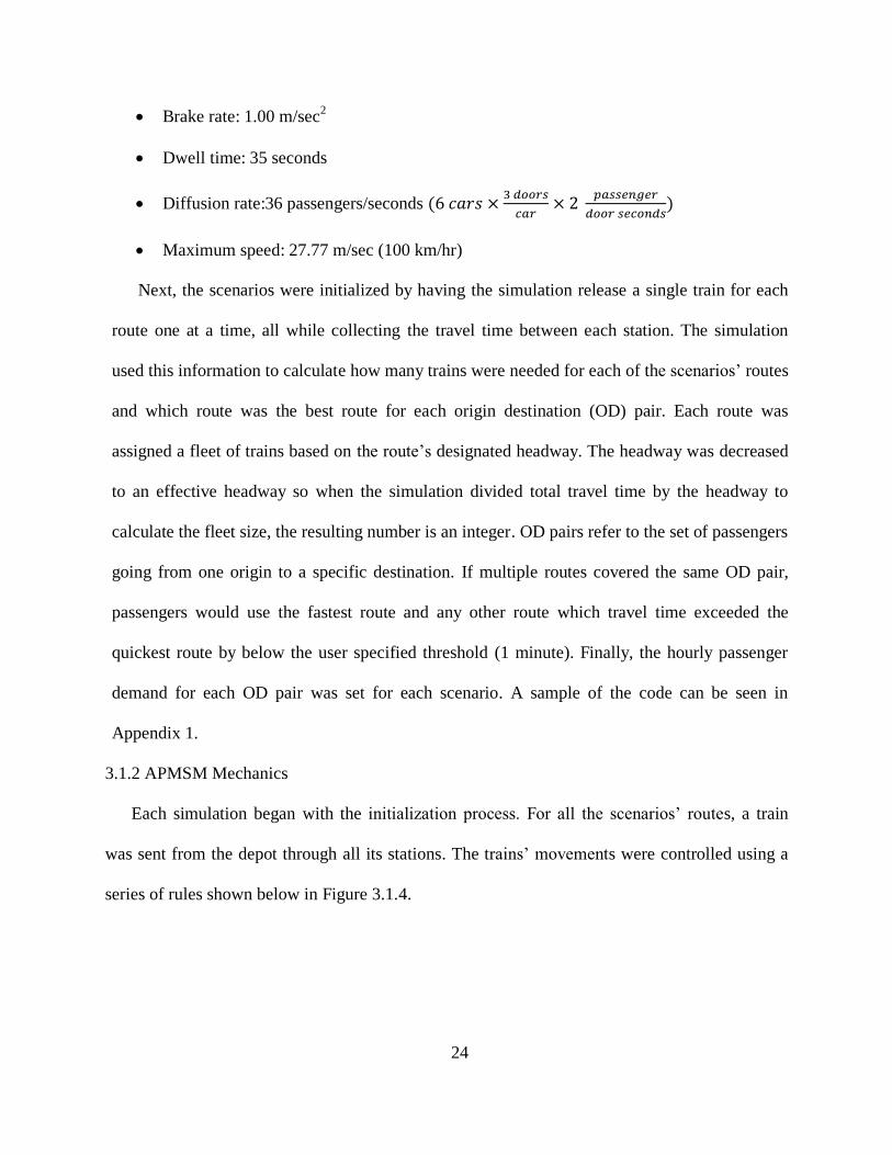
Each simulation began with the initialization process. For all the scenarios’ routes, a train
was sent from the depot through all its stations. The trains’ movements were controlled using a
series of rules shown below in Figure 3.1.4.
Page 33
25
Figure 3.1.4: Train Movement Rules
*If train is on curve, maximum velocity is calculated using equation 26.16 from Hay (1982)
While each train moved through the network, the simulation collected what time trains
arrived at each station (arrival to arrival). Once the train arrived at the first station of the route for
the second time, the train was removed from the system. The model calculated an effective
headway below the original headway based on the time it took the train to move through the
route. The initialization sequence created enough trains to support the effective headway. Using
this headway, the model assigned a start time to each train. This start time was adjusted in case
the initialize2 command was used. The run sequence began with each train leaving the depot
based on their assigned start time, ensuring that the trains were correctly spaced. Before the
official run sequence began, the simulation waited until all the trains were released from the
depot. The trains moved similarly to initializer trains with additional rules for stopped trains. See
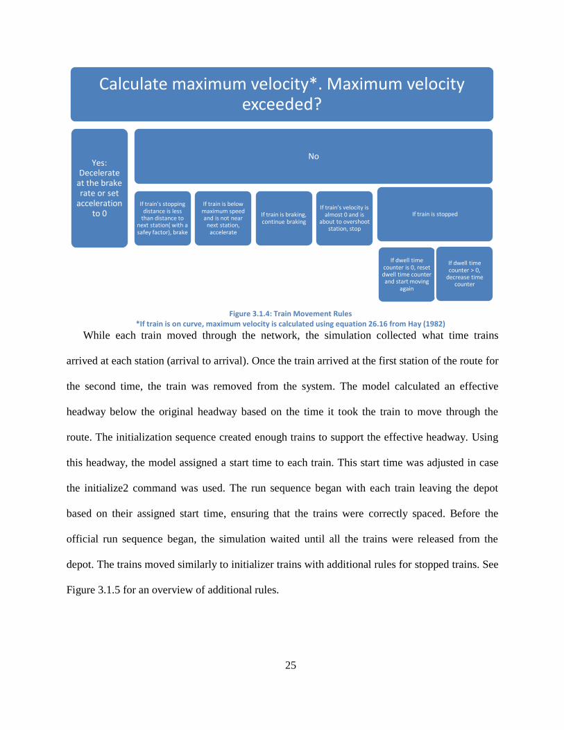
Figure 3.1.5 for an overview of additional rules.
Calculate maximum velocity*. Maximum velocity exceeded?
Yes: Decelerate
at the brake rate or set
acceleration to 0
No
If train's stopping distance is less
than distance to next station( with a safey factor), brake
If train is below maximum speed and is not near
next station, accelerate
If train is braking, continue braking
If train's velocity is almost 0 and is
about to overshoot station, stop
If train is stopped
If dwell time counter is 0, reset dwell time counter and start moving
again
If dwell time counter > 0,
decrease time counter
Page 34
26
Figure 3.1.5: Additional Dwell Rules for Run Sequence
The simulation could allow each train to go through a vehicle detection sequence that senses
if there is a vehicle in front, but this feature was disable in this thesis since the simulation
perfectly spaces vehicles and the operation was assumed to have no problems. After the
simulation ran for the set period of time (run time), the trains continued to operate until all
passengers reached their destination. After the run time was reached, the trains continued to
operate and record travel time, but all other simulation functions (wait time, passenger arrival,
etc.) were disabled, which prevented any skewing of the results. The entire simulation took
about 14 seconds to complete all the steps if all features were enabled. Disabling the vehicle
detection sequence and output file generation sped up the process considerably.
3.1.3 APMSM Output
APMSM outputted data in three locations: the Java console, the initializer text file, and the
train text file. The java console output contained information also included in the text files, but
the console output could be seen immediately after the simulation and did not require any
processing. The console information included a plethora of information, but most importantly,
Train is stopped
Is dwell time counter is between 1.5 seconds or the full dwell time -1.5 seconds. Is there people who need
to get out of the train?
Yes: A portion of train passengers exit
No: A portion of passengers waiting at the station enter the
train
Is dwell time counter less than 1.5 seconds or greater than full dwell
time - 1.5 seconds? Stay at station (Doors
opening and closing)
If dwell time counter is 0, reset dwell time counter and start
moving again
Page 35
27
the average wait time and average travel time. The initializer text file showed the initialization
trains’ activities, the travel time between each OD pair for each route, the direction between each
OD pair for each route, the minimum travel time between each OD pair, and the acceptable
directions between each OD pair. The train text file showed the same information from the
console in addition to the trains’ activity through the simulation and residual passengers waiting
at stations. When a completely new network was created for the thesis, all data sources were
reviewed to ensure their integrity, but when there were only minor adjustments, the console was
the only data source reviewed.
3.1.4 APMSM Assumptions
There are many assumptions built into APMSM that simplify the modeling process
including:
Stations and vehicles are represented as points
The system is two dimensional, the vertical component is neglected
Vehicles have constant acceleration
Trains operate perfectly (no breakdowns)
Passenger arrival is deterministic
Passengers are aggregated and when they move between stations and trains, an equal
proportion of passengers with the same origin/destination are moved between stations
and trains
For this thesis, intersections between other track sections were grade separated
All of the above assumptions differ to how automated people movers really operate, but
provided a good enough approximation for this thesis.
Page 36
28
3.2 PRT Simulation Methodology
BeamED, developed by Beamways AB, was the simulation tool utilized to model PRT.
BeamED allows users to draw a PRT network out of different elements by simply clicking on a
graphical user interface (GUI). These elements can be expanded or shrunk with simple key
strokes and any expansion or contraction to each element is reflected in the GUI. System
characteristics such as number of vehicles and maximum speed can be input in the setup menu.
Demand is specified with multiple techniques including an automatic population based demand
synthesizer, an OD table, or a land use based demand synthesizer. Once the simulation is
activated, it only takes a few seconds to model an hour’s worth of PRT operation. The model
assumes two-dimensional operation, deterministic passenger arrival, and perfect performance
just as APMSM. BeamED outputs data in a window after the simulation, through the elements
on the GUI, and on a spreadsheet stored in a separate file.
3.2.1 BeamED Input Requirements
To start each scenario, the network was drawn on the GUI. See Figure 3.2.1 for a screenshot
of the GUI.
Page 37
29
Figure 3.2.1: BeamEd Screenshot
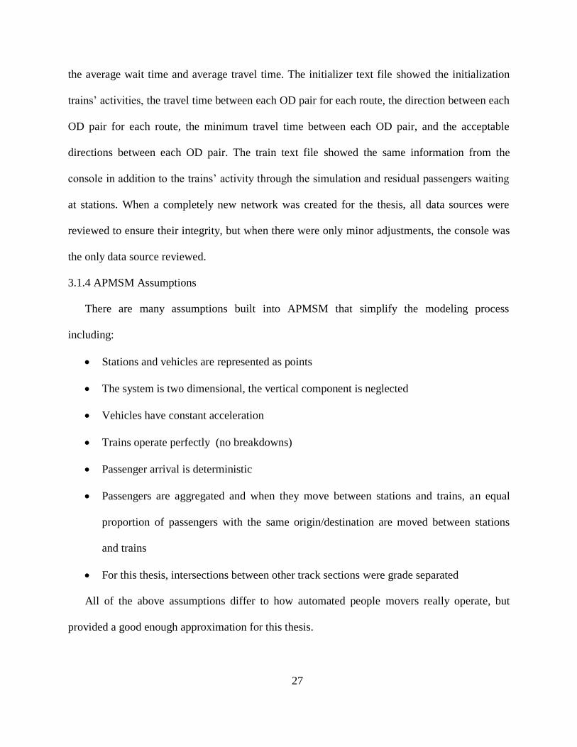
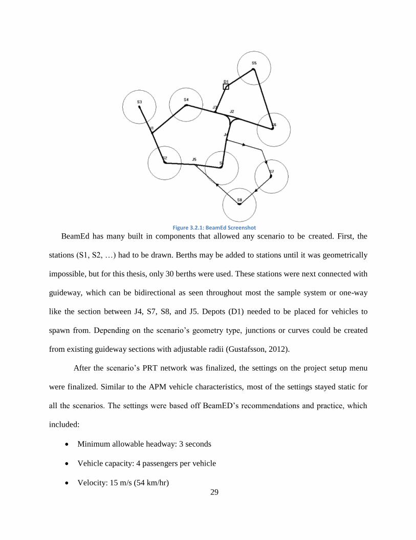
BeamEd has many built in components that allowed any scenario to be created. First, the
stations (S1, S2, …) had to be drawn. Berths may be added to stations until it was geometrically
impossible, but for this thesis, only 30 berths were used. These stations were next connected with
guideway, which can be bidirectional as seen throughout most the sample system or one-way
like the section between J4, S7, S8, and J5. Depots (D1) needed to be placed for vehicles to
spawn from. Depending on the scenario’s geometry type, junctions or curves could be created
from existing guideway sections with adjustable radii (Gustafsson, 2012).
After the scenario’s PRT network was finalized, the settings on the project setup menu
were finalized. Similar to the APM vehicle characteristics, most of the settings stayed static for
all the scenarios. The settings were based off BeamED’s recommendations and practice, which
included:
Minimum allowable headway: 3 seconds
Vehicle capacity: 4 passengers per vehicle
Velocity: 15 m/s (54 km/hr)
Page 38
30
Acceleration: 2.4 m/s2
Vehicle count: As needed
Simulation run time: 1 hour or 3600 seconds
Mean group size: 1.5 people per group
Although the upcoming Amritsar PRT will feature six-person vehicles, four-person vehicles
were used since they represent the industry standard (PRT Consulting, 2011). Demand was one
of the thesis’s settings that shift scenario to scenario. The simulation software has three
techniques to input demand. To implement the simplest method, only the population near the
PRT and the percentage of population that use PRT is needed. BeamEd automatically divides the
population proportionally based on the number of berths located at the station. This technique
provides a quick assessment of PRT, but does not take into account the type and magnitude of
activities around each station. Another method that can be utilized is inputting a demand matrix
with the number of riders between each station (OD Matrix). A demand matrix multiplier can be
applied to change the magnitude of the matrix if each cell in the matrix remains proportional to
one another. Lastly, GIS data can be utilized to estimate ridership based on the amount of
different population types (residential, work, shopping) in each GIS polygon. For this thesis, the
matrix technique was used because it allows the greatest control over demand levels (Gustafsson,
2012).
3.2.2 BeamEd Procedures
Less was known about the BeamEd procedures compared to APMSM since the
simulation code was unavailable to the public, but some of the important aspects of the
simulation were available. For most of the scenarios, BeamEd only took a few seconds to run,
but if the scenario was overcapacity, the system took longer to simulate. Through the course each
Page 39
31
simulation, the scenarios’ stations were assigned an ideal number of empty vehicles dwelled
based on the anticipated demand and the simulation would redistribute the vehicles around the
scenarios’ stations to match the ideal dwelled vehicle count. BeamEd used a pseudo dynamic
traffic assignment technique for vehicle route assignment where vehicles follow the shortest path
to their destination, which BeamEd recalculated every virtual five minutes for each origin
destination (OD) pair. BeamEd kept track of statistics throughout the simulations except during
the initial period of the simulation, when the system was stabilizing. The simulation behaved
similar to Group Rapid Transit (GRT). If there were not extra vehicles at a station, passengers
with the same destination were modeled to share the same vehicle, though this happened more
during scenarios with heavy loads (Gustafsson, 2012).
3.2.3 BeamEd Output
BeamEd has three sources of information, a window that displays after the simulation
finishes, the simulation network itself (result display) and a spreadsheet. The window provides a
quick overview of network geometry, network performance, vehicle performance, and passenger
delay. The result display shows the performance of the simulation network and how each
component performs during the simulation. A sample result display output is shown below in
Figure 3.2.2.
Page 40
32
Figure 3.2.2: Sample Result Display
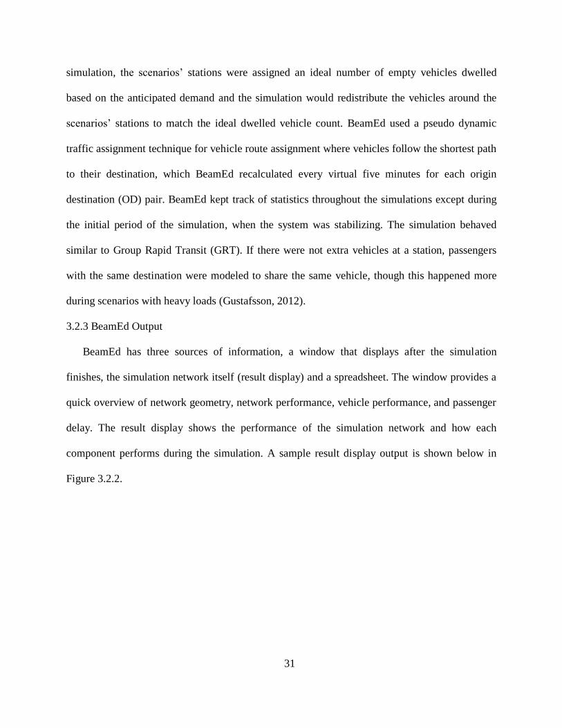
The thickness of the guideway sections represents the usage of the tracks. If they are colored
red, the usage is above half the capacity. Each station has a corresponding pie chart. The larger
the chart, the greater the station usage was. For each of the pie charts, red and yellow represent
the ratio of arrivals and departures respectively. The cursor may be moved over the station area
to obtain station specific information such as number of berths, maximum number of passengers
waiting, or the number of arrivals per hour. Junctions are not full designed before the simulation
starts, but after the simulation trial, the model will show what type of junction should be
constructed for each intersection. If the junction is not too busy, it can be built as a roundabout as
shown by a circle (J2). If the junction has higher volumes, it should be built as a cloverleaf,
which is represented as a 3 or a 4 depending on how many legs the junction has. The spreadsheet
displays the same information as the window with the addition of many origin and destination
matrices including travel time and average speed. For this thesis, the average wait time from the
window and travel time matrix from the spreadsheet were the most pertinent information.
Page 41
33
3.2.4 BeamEd Assumptions
Multiple assumptions were made in the mechanics of BeamEd. They include:
The system is two dimensional, the vertical component is neglected
Trains operate perfectly (no breakdowns)
Passengers share vehicles if they have the same destination and if there is a queue
Group size is based on discretized Poisson Distribution with selected mean
Arrivals are deterministic, but pulse arrivals can be programed
3.3 Measures of Effectiveness
The main measure of effectiveness (MOE) for the thesis was average trip time. Average trip
time is the sum average wait time and average travel time, which are both outputs from each of
the simulation programs. Decision makers choosing which mode to implement for a new transit
project consider the lifecycle costs, reliability, and environmental impacts in addition to trip
time. These other MOEs were not considered because they were either too system-specific or
about the same between APM and PRT.
Lifecycle costs, which include capital and annual costs, are generally the most important
MOE to decision makers, especially when budgets are limited. Cost greatly varies based on the
location of a transit system. Capital and annual costs depend on:
Material expenses- Material expenses can vary by location
Terrain/environment of the project- The terrain/environment can require certain
additions( tunnels, viaducts, bridges, site remediation, traffic impact mitigations, etc.) that
greatly increase the cost
Project’s jurisdiction’s code/laws: Labor laws, building codes, document requirements,
and the permitting process varies by the nature and location of the project
Page 42
34
Labor costs: Labor costs vary considerably region to region
All the above factors contribute in making an APM or PRT system with the exact same
alignment cost much different in one location verses another. Per mile and station costs estimates
are available such as the figures used in Juster and Schonfeld (2013), but PRT is overwhelmingly
less expensive. See Chapter 6, Application, for a cost comparison of two actual systems.
Service reliability, defined here as the percent of time the system operates without an
operational problem, is another important MOE. If a system does not work when it is needed,
there is little reason to build it. Reliability is high dependent on the quality of the system’s
construction and how well a system is maintained. Both APM and PRT have proven to operate
with reliabilities above 99% (Long, 2011; TransLink, 2011). Since both modes are
extraordinarily reliable, there was not a reliability difference to compare for each scenario.
In terms of environmental impacts, both PRT and APM use about the same amount of
energy, but what environmental impacts are considered is contingent on a transit project’s
location. An automated guideway transit system located in a busy downtown area would need to
be designed to minimize the visual impact, while a system in a suburban center filled with homes
would have to attempt to minimize noise. For an exterior airport automated guideway transit
systems, noise or visual impacts are generally not considered.
Page 43
35
Chapter 4: Simulation Trials Description
Multiple simulations were performed to model what type of systems would appear in
airports, specialized activity centers or urban areas. Multiple system designs types were analyzed
and cover a spectrum of alignment designs and magnitudes. The demand levels and distributions
were adjusted to cover a wide range of situations. The various geometric and demand situations
were combined to form final testing scenarios for both APM and PRT.
4.1 System Design Types
The first and simplest design type was dual lane, which is fundamentally a linear route.
Notable linear routes include Atlanta Airport’s Plane Train, Dubai Metro’s Red Line, and the Las
Vegas Monorail. These types of routes may be component within with a larger network, but
linear routes operate independently on their own right of way. The Y-type of route resembles a
linear route, but has another segment that branches out usually towards the end of the route. The
London Heathrow PRT, Copenhagen Metro, and the Canada Line of the Vancouver Skytrain
system all resemble a Y-type system. The Y-type system features two routes that share tracks on
part of their journey, but diverge on one end of track to go their separate ways. The loop type of
system appears to be a linear route whose ends are connected to form a circle. The Detroit People
Mover, Seattle Tacoma Airport’s Satellite Transit System, and Dallas Fort Worth Airport’s
Skylink are all loop systems. Some loop type routes are bi-directional and others are one-way.
The last type of system was loop with legs and looks like the loop system with branches out the
loop. Notable loop with legs type system include the Airtrain JFK, Miami Metromover, and the
Airtrain SFO. Figure 4.1.1 shows maps for each type of system.
Page 44
36
Source: Las Vegas Monorail, 2013
System: Las Vegas Monorail
Type: Linear
Source: Mapsof.net, 2012
System: Copenhagen Metro
Type: Y
Source: Drdisque, 2006
System: Detroit People Mover
Type: Loop
Source: Miami Dade County, 2012
System: Miami Metromover
Type: Loop with Legs Figure 4.1.1: System Design Examples
4.2 Geometric Alterations
Transit systems vary in how far apart stations or stops are. Local buses may have stops every
block, while commuter rail services can have miles between each station. Light rail or heavy rail
systems such as the Washington Metro or Miami Metrorail, have station placed close to each
other in downtown center, but far apart towards the suburban areas. Transit located in activity
centers generally has roughly equidistant station spacing. Transit systems’ varying station
spacing can be demonstrated by the Miami Metromover APM system and Miami Metrorail
heavy rail system shown below in Figure 4.2.1.
Page 45
37
Figure 4.2.1: Miami’s Urban Rail Systems
Source: (Sharemap.org, 2013)
Miami has three passenger rail systems including Tri-Rail, Miami Metromover, and Miami
Metrorail. Tri-Rail is a commuter system that spans multiple counties and is out of scope for
PRT. Miami Metromover, the purple system circled in Figure 4.2.1 and shown on the lower right
of Figure 4.1.1, is an APM located in the central business districts of Miami. This system was
built to transport people around the busy commercial hub and many of the Metromover
passengers feed into the Metrorail system (Brooks, 1989). Metromover stations are very close to
each other at about 0.2 miles apart. Miami Metrorail, the red and yellow system that spans Figure
4.2.1, is a heavy rail system that spans Miami-Dade County. It facilitates movement from
Page 46
38
Miami-Dade County’s residential areas to the urban core. Metrorail’s station spacing varies from
less than half a mile in the downtown area to more than a mile in the more residential areas. For
this thesis, each system design was additionally adjusted by increasing or decreasing distance
between stations (station spacing). For most of the scenarios the stations were equally spaced
apart, but in some scenarios, the station spacing varied. This action reflects how different transit
systems (Miami Metromover vs. Metrorail) have different station spacing. Stations were spaced
0.25, 0.5, 1, and 2 miles apart. Half the 1 mile station spacing scenarios also varied station
spacing to reflect an urban to suburban system such as Miami Metrorail (except loop scenarios)
and include 0.5, 1, and 2 mile apart stations all in the same network. In addition, the number of
stations per route included 5, 10, and 20 stations per route.
4.3 Demand Levels
Transit systems with the same technology generally have the same capacity, but have quite
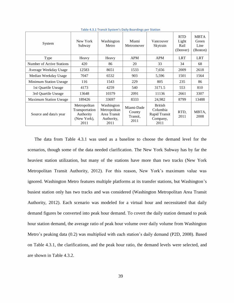
different utilization. Table 4.3.1 shows a few different transit system and statistics about their
utilization.
Page 47
39
Table 4.3.1 Transit System’s Daily Boardings per Station
System New York
Subway
Washington
Metro
Miami
Metromover
Vancouver
Skytrain
RTD
Light
Rail
(Denver)
MBTA
Green
Line
(Boston)
Type Heavy Heavy APM APM LRT LRT
Number of Active Stations 420 86 20 33 34 68
Average Weekday Usage 12583 8651 1533 7,656 2009 2618
Median Weekday Usage 7047 6532 903 5,596 1501 1564
Minimum Station Useage 116 1543 229 805 235 86
1st Quartile Useage 4173 4259 540 3171.5 553 810
3rd Quartile Useage 13648 10379 2091 11136 2661 3307
Maximum Station Useage 189426 33697 8333 24,982 8799 13488
Source and data's year
Metropolitan
Transportation
Authority
(New York),
2011
Washington
Metropolitan
Area Transit
Authority,
2011
Miami-Dade
County
Transit,
2011
British
Columbia
Rapid Transit
Company,
2011
RTD,
2011
MBTA,
2008
The data from Table 4.3.1 was used as a baseline to choose the demand level for the
scenarios, though some of the data needed clarification. The New York Subway has by far the
heaviest station utilization, but many of the stations have more than two tracks (New York
Metropolitan Transit Authority, 2012). For this reason, New York’s maximum value was
ignored. Washington Metro features multiple platforms at its transfer stations, but Washington’s
busiest station only has two tracks and was considered (Washington Metropolitan Area Transit
Authority, 2012). Each scenario was modeled for a virtual hour and necessitated that daily
demand figures be converted into peak hour demand. To covert the daily station demand to peak
hour station demand, the average ratio of peak hour volume over daily volume from Washington
Metro’s peaking data (0.2) was multiplied with each station’s daily demand (P2D, 2008). Based
on Table 4.3.1, the clarifications, and the peak hour ratio, the demand levels were selected, and
are shown in Table 4.3.2.
Page 48
40
Table 4.3.2: Scenario Demand Levels
Loading Daily
Passengers
Peak Hour
Passengers
Very Low (Miami
Metromover) 1000 200
Low (Light rail) 2500 500
Medium (Skytrain) 5000 1000
High (Heavy Rail) 7000 1400
4.4 Demand Distribution
For the scenarios with equal station spacing, the same peak hour passenger levels were used
for each station. When there was unequal station spacing, additional demand was allocated based
on a typical suburban to urban morning commute pattern. The stations that were 2 miles apart
would be considered stations on toward the edge of the system and have mostly passengers
commuting elsewhere in the morning. The stations 1 mile apart were considered suburban
stations with passengers commuting to and from the station in the morning. Stations 0.5 miles
apart were considered urban core stations that mostly draw in morning passengers. Using
Washington Metro OD information for morning commutes, another OD table was created , as
seen on Table 4.1.1., with the median number of passengers for a given combination of edge (E),
suburban (S), and urban (U) origin destination combination (P2D, 2008).
Table 4.4.1: Washington Metro Median Outer Suburban Core Origin Destination Combination
Destination
Ori
gin
C S E
C 25.91 6.36 2.55
S 35.64 2.41 7.20
E 53.09 10.00 3.50
To compute the final OD numbers for the unequally spaced stations, the following equation
was used.
Page 49
41
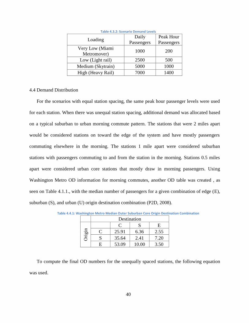
∑ ∑
X=Number of Passengers for a certain origin (O) and destination (D)
T=Total number of passengers in the system (=Number of stations * 200)
D=Demand from Table 4.1.1
N= Number of the OD type in the system
M= Multiplier (1, 2.5, 5, 7 depending on if the base number of passengers per stations is 200,
500, 1000, or 1400)
4.5 Combining Variables
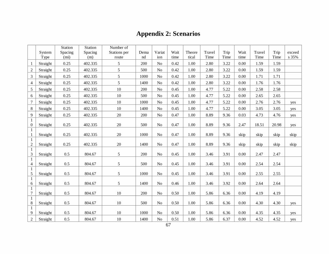
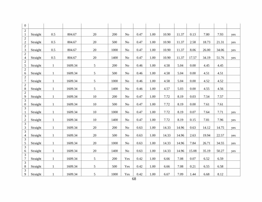
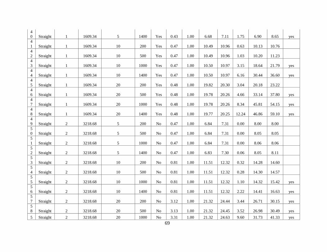
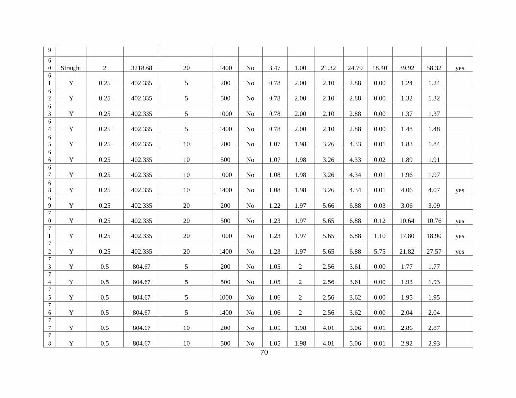
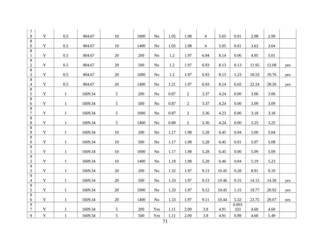
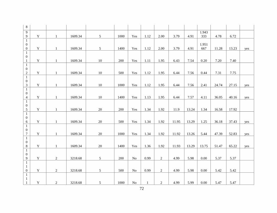
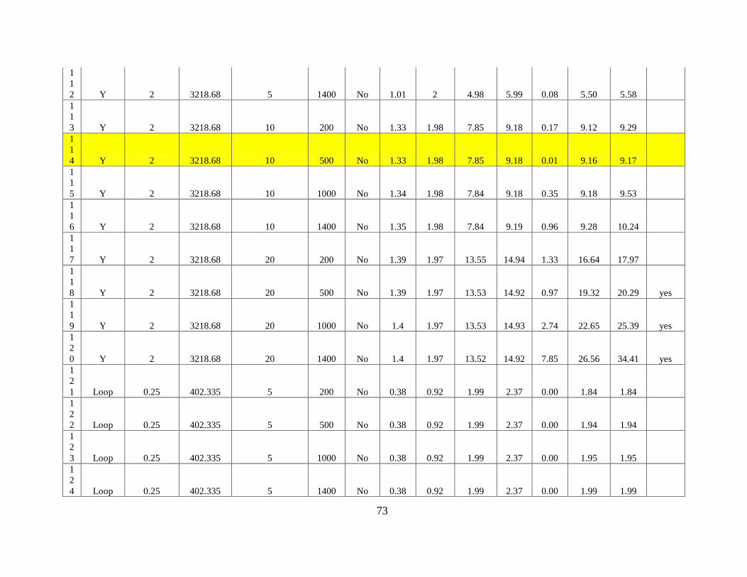
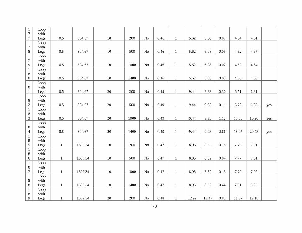
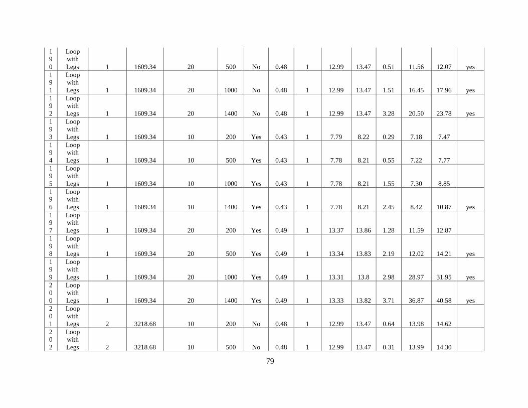
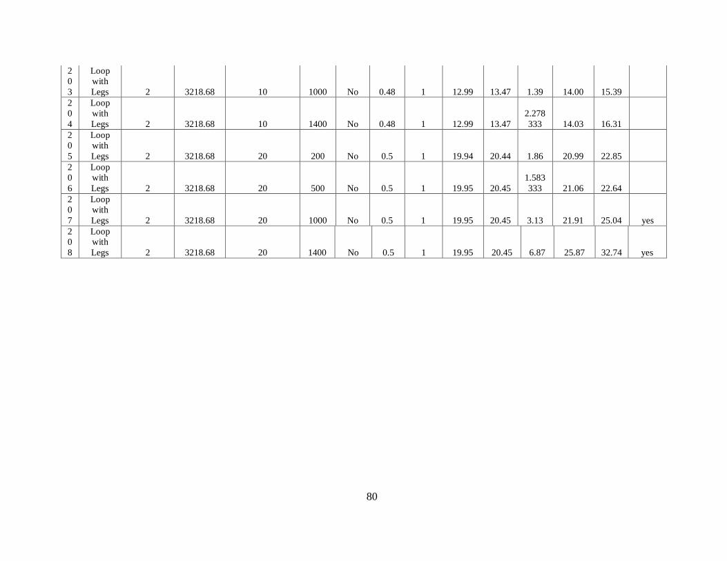
Combining all the possible independent variables led to the creation of 208 scenarios. Each
scenario was tested on both the APM and PRT simulation. See Appendix 2 for all the scenarios
and their results.
Page 50
42
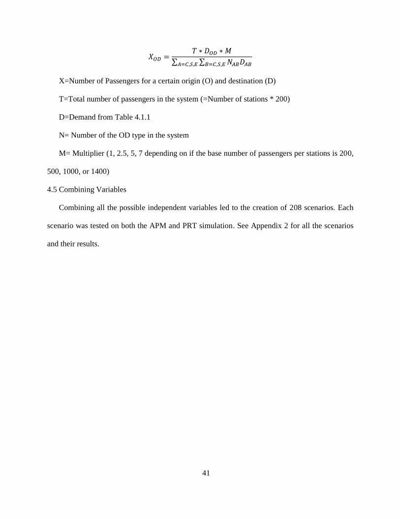
Chapter 5: Simulation Results
The results are displayed below using a graph matrix for each system design. Due to space
constraints of the graph matrices, the legend, axes labels, and graph title are taken out of each
graph. A sample of a graph with the missing information is shown below in Figure 5.0.1.
Figure 5.0.1: Results Graph Example
The x-axis represents passengers per station per hour and the y-axis shows average trip time
per passenger. The dashed line with diamonds symbolizes APMs while the solid line with
squares represents PRT. Since the distances between stations and number of stations were also
varied, the graphs within each of the system design’s matrix are arranged accordingly. Each row
of graphs has the same spacing between stations and each column had the same number of
stations.
0.00
20.00
40.00
60.00
80.00
0 500 1000 1500
Ave
rage
Tri
p T
ime
(Min
ute
s)
Passengers Per Station Per Hour
Dual Lane with 20 Station at 2 miles Apart
APM
PRT
Page 51
43
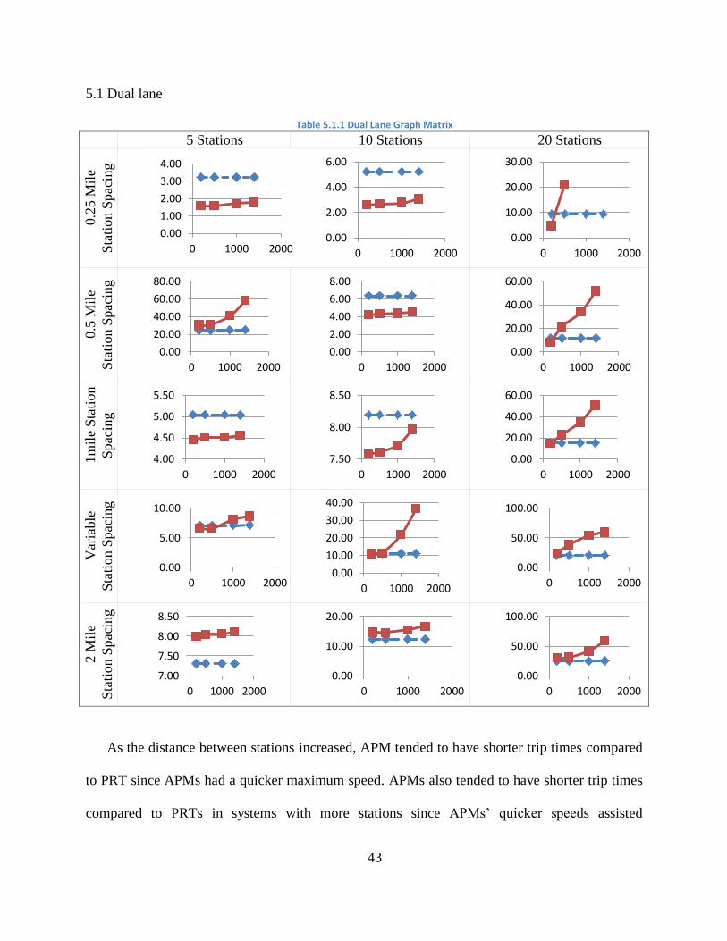
5.1 Dual lane
Table 5.1.1 Dual Lane Graph Matrix
5 Stations 10 Stations 20 Stations
0.2
5 M
ile
Sta
tion S
pac
ing
0.5
Mil
e
Sta
tion
Spac
ing
1m
ile
Sta
tion
Spac
ing
Var
iable
Sta
tion S
pac
ing
2 M
ile
Sta
tion S
pac
ing
As the distance between stations increased, APM tended to have shorter trip times compared
to PRT since APMs had a quicker maximum speed. APMs also tended to have shorter trip times
compared to PRTs in systems with more stations since APMs’ quicker speeds assisted
0.00
1.00
2.00
3.00
4.00
0 1000 20000.00
2.00
4.00
6.00
0 1000 2000
0.00
10.00
20.00
30.00
0 1000 2000
0.00
20.00
40.00
60.00
80.00
0 1000 2000
0.00
2.00
4.00
6.00
8.00
0 1000 2000
0.00
20.00
40.00
60.00
0 1000 2000
4.00
4.50
5.00
5.50
0 1000 2000
7.50
8.00
8.50
0 1000 2000
0.00
20.00
40.00
60.00
0 1000 2000
0.00
5.00
10.00
0 1000 20000.00
10.00
20.00
30.00
40.00
0 1000 2000
0.00
50.00
100.00
0 1000 2000
7.00
7.50
8.00
8.50
0 1000 2000
0.00
10.00
20.00
0 1000 2000
0.00
50.00
100.00
0 1000 2000
Page 52
44
passengers traveling longer distances and APMs’ greater capacity could handle the increased
number of passengers from the additional stations. PRT’s time advantage shank as the number as
the passenger demand per station grew. An extreme example of this trend was with the 20 station
system with 0.25 miles between each station. PRT was much quicker than APM with 200
passengers per station, but the time advantage eroded so quickly, that the 1000 and 1400
passengers could not be practically modeled for PRT (thus not appearing on the graph). PRT
likely failed in this system with higher passenger counts because the tracks were saturated with
vehicles. Systems with larger spacing between stations had more room for more vehicles. Figure
5.1.1 shows the flow of PRT vehicles (and passengers in APM’s case) for the dual lane
configuration.
Figure 5.1.1: Dual Lane Configuration Flow
As a general trend, the middle of the system was the busiest location since any passengers
trying to move from one half of the system to the other half had to go through the center. In
PRT’s case, this resulted in congestion of the guideway and for APM, the vehicles themselves
became more crowded.
When the unequal station spacing systems were modeled, APM generally performed better.
That was because APMs’ greater capacity can accommodate the unidirectional flow of the
Page 53
45
suburban to urban commuting pattern seen in Figure 5.1.2, which concentrated passenger flow
towards the urban stations.
Figure 5.1.2: Dual Lane Unequal Station Spacing Flow
Moving left to right from the edge stations towards the urban stations, the route became
congested (i.e., volume approached capacity) by the third edge station. Some of the congestion
was relieved by the start of the suburban stations as some of the edge passengers exited at
suburban station. This relief was temporary and by the last suburban station, congestion
reappeared. Most of the congestion was relieved after half of the urban-bound edge and suburban
commuters exited at the first urban station.
5.2 Y
All the Y configuration systems had one fifth of the stations in the stem and two fifth of the
stations in the branches which were spaced thirty degrees apart. Since the branches were almost
parallel and movement between the branches required a considerable distance away from one’s
destination, there were no passengers that traveled from one branch to the other branch. The
APM Y systems required 2 routes to cover all the station. Each route covered the stem and one
of the branches. The headway of both routes was 4 minutes to ensure that the headway in the
stem had the minimum allowable headway of 2 minutes.
Edge | Suburban | Core
Page 54
46
Table 5.2.1 Y Graph Matrix
5 Stations 10 Stations 20 Stations
0.2
5 M
ile
Sta
tion
Spac
ing
0.5
Mil
e S
tati
on
Spac
ing
1m
ile
Sta
tion S
pac
ing
Var
iable
Sta
tion
Spac
ing
2 M
ile
Sta
tion
Spac
ing
0.00
1.00
2.00
3.00
4.00
0 1000 2000
0.00
2.00
4.00
6.00
0 1000 2000
0.00
10.00
20.00
30.00
0 500 1000 1500
0.00
2.00
4.00
0 1000 2000
0.00
2.00
4.00
6.00
0 500 1000 1500
0.00
10.00
20.00
30.00
0 500 1000 1500
0.00
2.00
4.00
6.00
0 1000 2000
0.00
5.00
10.00
0 1000 2000
0.00
20.00
40.00
0 1000 2000
0.00
5.00
10.00
15.00
0 1000 2000
0.00
20.00
40.00
60.00
0 1000 2000
0.00
50.00
100.00
0 1000 2000
5.00
5.50
6.00
6.50
0 1000 2000
9.00
9.50
10.00
10.50
0 1000 2000
0.00
20.00
40.00
0 1000 2000
Page 55
47
The Y system configuration performed similarly to the dual lane configuration with APM
performing better with more stations (especially with high passenger demand) and smaller
spacing between stations, except PRT tended to perform better in the Y configuration compared
to APM. This was most likely due to the shorter trip lengths. For the 2 mile 0.5 mile station
spacing system, the longest possible trip for a 20 station 2 mile spacing system was 40 miles and
22 miles for a dual lane and Y configuration respectively. The short trip distances made PRT’s
slower speeds less of an issue. The traffic flow for Y configuration systems can be seen in Figure
5.2.1.
Figure 5.2.1 Y Configuration Flow
The Y configuration tended to be more crowded towards the center system. The most
congested region of the Y was where the stem met the junction since the traffic from the two
branches created a bottleneck effect. Even though the beginning of each branch was expected to
have major congestion as well, those sites only has minor congestion, possible due to the
additional capacity of the adjacent junction and the additional capacity of having two sets of
tracks for the branches as opposed to the stem’s one set of tracks.
Page 56
48
Figure 5.2.2 Y Unequal Station Spacing Flow
Based on Figure 5.2.2, the Y unequal station spacing configuration had congestion at similar
locations as the dual lane unequal station spacing system, though the branches at the junction
with the stem was less congested than expected.
5.3 Loop
No variable spacing versions of the loop configuration were tested because loop systems
generally have uniform spacing. An unequal spacing system was created with the loop with legs
configuration. The loop had two routes each with 2 minute headway, one serving all the station
clockwise and the other route serving all the stations counter-clockwise.
Core | Suburban | Edge
Page 57
49
Table 5.3.1: Loop Graph Matrix
5 Stations 10 Stations 20 Stations
0.2
5 M
ile
Sta
tion
Spac
ing
0.5
Mil
e S
tati
on
Spac
ing
1m
ile
Sta
tion S
pac
ing
2 M
ile
Sta
tion
Spac
ing
The loop configuration had lower trip times for both APM and PRT compared to the Y
configuration with small station spacing (0.25 & 0.5 miles). This was caused by the greater
connectivity and redundancy of having two ways to reach a destination. The loop
configuration’s time advantage diminished once the station spacing was 1 or 2 miles between
stations, especially for PRT which by comparison, tended to perform less favorably compared
0.00
1.00
2.00
3.00
0 1000 2000
0.00
2.00
4.00
6.00
0 1000 2000
0.00
10.00
20.00
0 1000 2000
2.70
2.80
2.90
0 1000 2000
4.20
4.40
4.60
4.80
0 1000 2000
0.00
10.00
20.00
0 1000 2000
0.00
2.00
4.00
6.00
0 1000 2000
6.00
6.50
7.00
7.50
0 1000 2000
0.00
10.00
20.00
0 1000 2000
0.00
5.00
10.00
0 1000 2000
0.00
5.00
10.00
15.00
0 1000 2000
0.00
20.00
40.00
0 1000 2000
Page 58
50
APM, which is exemplified when station spacing was 1 or 2 miles and the system had 10 or 20
stations. With these scenarios, PRT performed generally better than APM for the Y
configuration, but APM always performed better with a loop configuration. APM performed
better than PRT probably because each OD pair tended to have fewer intermediate stations and
each OD pair utilized an APM route with 2 minute headways. Figure 5.3.1 shows a 20 station
loop configuration. The branches off the loop are depots and do not affect the performance of the
system.
Figure 5.3.1: Loop Configuration Flow
The loop configuration has uniform traffic around the system, which is intuitive since no
matter which station is chosen, the system appears identical relative to the station.
5.4 Loop with Legs
The loop with legs configuration was constructed with 4/10 of the stations located in the loop
section of the system and 3/10 of the stations located at each of the legs which are 30 degrees
apart. There were also two junctions in the loop section spaced the same distance apart as the
stations. Five station scenarios were neglected because five stations were too few to create a loop
Page 59
51
with loop system. Just as the loop configuration, travel between the legs was neglected. There
were two two minute headway routes. One that served the stations of one of the branches and the
all the loop stations clockwise, and the other route served the other branch and all the loop
stations counterclockwise.
Page 60
52
Table 5.4.1 Loop with Legs Graph Matrix
10 Stations 20 Stations
0.2
5 M
ile
Sta
tion
Spac
ing
0.5
Mil
e S
tati
on
Spac
ing
1m
ile
Sta
tion S
pac
ing
Var
iable
Sta
tion
Spac
ing
2 M
ile
Sta
tion S
pac
ing
0.00
2.00
4.00
6.00
0 500 1000 1500
0.00
10.00
20.00
30.00
0 500 1000 1500
0.00
5.00
10.00
0 500 1000 1500
0.00
10.00
20.00
30.00
0 500 1000 1500
7.50
8.00
8.50
9.00
0 500 1000 1500
0.00
10.00
20.00
30.00
0 500 1000 1500
0.00
5.00
10.00
15.00
0 500 1000 1500
0.00
20.00
40.00
60.00
0 500 1000 1500
0.00
10.00
20.00
0 500 1000 1500
0.00
20.00
40.00
0 500 1000 1500
Page 61
53
The loop with legs configuration was generally slower than the loop and Y configuration, but
faster than the dual lane configuration. This configuration favored PRT more heavily compared
to any other configuration since the loop leg configuration had the most complexity of any
scenario and complexity added redundancy. This redundancy gave PRT vehicles more flexibility
when moving throughout the system. Compared to other configurations, loop with leg’s PRT
system’s trip time increased at proportionally the slowest rate. The loop with leg configuration
flow can be seen in Figure 5.4.1.
Figure 5.4.1 Loop with Legs Configuration Flow
The loop with leg configuration’s congestion was primarily located where the legs at the
loop intersect. An unequal station spacing system can be seen in Figure 5.4.2.
Page 62
54
Figure 5.4.2: Loop with Leg Unequal Station Spacing Flow
Compared to other configurations, loop with leg’s unequal spacing system performed
more favorability towards PRT, though APM was still the quickest mode for the 1000 and 1400
passenger per station per hour scenarios. As with the equal spacing system, most of the
congestion was located where the loop and legs intersect.
5.5 Overall
In the simulations, PRT tended to perform better than APM if the system was complex
and had fewer stations closer apart. Longer trip distances from additional stations placed further
apart made PRT’s slower maximum speed an obstacle for providing quicker trips. Additional
stations do not necessarily make PRTs slower, but the additional passengers from the additional
stations without additional system capacity proved to be a problem. If the PRT system is
designed with redundant paths for each OD pair such as the system shown in Figure 1.2.1, PRT
would be able to increase system capacity. This could be a problem for real-life implementation
since extra connections would be extra construction costs.
Edge | Suburban | Urban
Page 63
55
Chapter 6: Application
The tables generated in Chapter 5 can be used to quickly evaluate whether APM or PRT is
the faster mode. Below are two examples of using the tables to choose the faster mode.
6.1 PHX Sky Train
The PHX Sky Train™ is an APM whose first phase opened in April 2013 at Phoenix
SkyHarbor International Airport and will eventually connect parking, the rental car center,
several terminals, and a light rail line that goes through the Phoenix area. See Figure 6.1.1 for
the APM alignment.
Figure 6.1.1 PHX Sky Train™ Alignment Source: Phoenix Sky Harbor Airport (2013)
Based off the information and assumptions supplied by Sky Harbor, once the second phase
of the PHX Sky Train™ is completed it will (Phoenix Sky Harbor Airport, 2013):
Be a straight alignment
Have 5 stations placed about 1 mile apart
Page 64
56
Accommodate 670 passengers per hour during the peak (assuming 8% of daily
passengers use system during peak and uniform station demand)
Based off Table 5.1.1, a PRT version of this system will have an average trip time of about
4.51minutes per passenger while the APM version would have an average trip time of 5.04
minutes per passenger. The average trip times are not very different, but when considering that
London Heathrow PRT built in a similar environment only cost about $16.2 million per mile and
the PHX Sky Train™ is estimated to cost $322 million per mile, PRT’s slightly better trip time is
an additional advantage beyond the possible cost savings (Juster & Schonfeld, 2013; Phoenix
Sky Harbor Airport, 2013).
6.2 Detroit People Mover
The Detroit People Mover is an underutilized APM that opened in 1987, and circulates
visitors and workers around Detroit’s central business district. A map of the APM can be seen in
Figure 4.1.1. Since opening, it has been considered a white elephant (Aitken & Barker, 1989).
The Detroit People Mover has:
A loop alignment (in reality, it is a one-way loop, but for this application it will be
represented as if it was a two-way loop)
13 stations placed roughly 0.25 miles apart (Detroit Transportation Corporation, 2008)
461 passengers per station per day (Milwaukee Daily Reporter, 2011)
Based off Table 5.3.1, the average trip time would be 3.86 and 2.80 minutes per passenger
for APM and PRT respectively. Though these two low traffic examples favored PRT, any
heavily utilized urban system such as Washington D.C. or New York City’s subway would favor
APM.
Page 65
57
Chapter 7: Post Simulation Analyses
Many assumptions were made when using both the simulations including the maximum
velocity and acceleration/ brake rate of the vehicles. Though the capacity of PRT was often
exceeded during simulation, all APM scenarios had adequate capacity. These simulated
capacities might not have been reasonable to the theoretical or empirical capacities. Travel time
and wait time were added together for the results, but demand can affect each type of time
differently. In this chapter, the assumptions’ effects on the results were tested, different types of
capacity for both systems were quantified, and each time’s sensitivity to demand was tested for
each mode.
7.1 Velocity
A change in the maximum velocity has the potential to affect the results. Greater maximum
velocity can decrease travel time, but the magnitude of the change might differ for the two
modes. Using the dual lane 10 station variable spacing/demand scenario with 200 passengers per
station, the effect of the maximum velocity was evaluated. This particular scenario was chosen
because there was only a 13 second difference in average trip time between the modes and the
variable spacing will mitigate the influence of station spacing on the results. The results can be
seen below in Figure 7.1.1.
Page 66
58
Figure 7.1.1: Maximum Velocity’s Effect on Trip Time
Maximum velocity did significantly affect the average trip time per person, but each mode
was affected at a different magnitude. Both modes’ trip times decreased due to faster speeds, but
at some point, this increase was limited by acceleration. If the maximum velocity was high
enough, the vehicle did not have enough time to reach the maximum velocity since the
acceleration and break rate was not increased with velocity. APM’s time advantage with
increasing velocities was also limited by the dwell time each station, unlike PRT which does not
have intermediate stations to limit the distance within each trip for vehicles to reach the
maximum velocity. When maximum velocity decreased, both modes’ trip times increase at a
higher magnitude than the trip times decreased with increasing the maximum velocity. The
increase in trip time was more prominent in PRT since at 50% maximum velocity, APM velocity
was 1.85 times greater than PRT and the APM’s dwell time became a less significant factor in
the overall trip time since the vehicles moved so slowly.
0
5
10
15
20
25
30
35
40
45
0% 100% 200% 300% 400%
Ave
rage
Tri
p T
Ime
Per
Pas
sen
ger
(Min
ute
s)
Percent of Original Maximum Velocity
APM (27.77 m/s)
PRT (15 m/s)
Page 67
59
7.2 Acceleration/ Brake Rate
The same scenario used in section 7.1 was used for testing acceleration/ brake rate. The
results can be seen in Figure 7.2.1
Figure 7.2.1: Acceleration/Brake Rate’s Effect on Trip Time
Similarly to maximum velocity, increasing the acceleration/brake rate decreased the average
trip time and vice versa. Unlike maximum velocity, APM was much more sensitive to a change
in acceleration than PRT because APMs have to start and stop many times for each trip unlike
PRT which only has to start and stop once.
7.3 Capacity
Line capacity is the number of passengers in vehicles that can pass through a single point
per time unit. There are three ways to estimate capacity:
Empirical- What the capacity of actual systems are
Theoretical- Mathematically what the capacity of systems should operate at assuming full
loads, and neglecting acceleration and braking
Simulated- The approximate capacity estimated through simulation
0
2
4
6
8
10
12
14
16
18
0% 100% 200% 300% 400%
Ave
rage
Tri
p T
Ime
Per
Pas
sen
ger
(Min
ute
s)
Percent of Original Acceleration/Brake Rate
APM (1 m/s2)
PRT (2.4 m/s2)
Page 68
60
Each type of capacity for APM and PRT can be seen in Table 7.3.1.
Table 7.3.1: Capacities of APM/ PRT (Passengers per Hour per Direction)
Mode Empirical Theoretical Simulated
APM 25,000 (Shen, Zhao,
& Huang, 1995) 24,120 28,000
PRT * 4,800 4,800 *There is not enough PRT empirical capacity data
To calculate the theoretical capacity of each mode the below equation was used.
(
)
The simulated capacity was estimated by modeling two stations one mile apart. The APM
simulated capacity was above the theoretical capacity since the effective headway (the headway
that allows for perfect spacing between vehicles) was below the 120 second headway used in the
theoretical calculation. PRT had its system capacity near or equivalent to the theoretical capacity,
but APM’s theoretical capacity is less than the empirical capacity and the theoretical capacity
exceeds the empirical capacity. The simulated scenarios represent perfect operations, but transit
systems rarely (and almost never) operate with perfect conditions. The empirical capacity was
below the theoretical capacity because the empirical study’s APM system used a headway below
two minutes. A possible area of study is how sub-optimal operating conditions affect each of the
automated guideway transit types’ operation. Also, each of the simulators could have typical
operational issues built in to adjust the capacity to more practical levels.
7.4 Sensitivity of Travel Time to Demand
The graph matrices in Chapter 5 show trip time in comparison to demand. In Figures 7.4.1
and 7.4.2, the effect of changing demand on travel and trip time is shown for PRT and APM. A
loop with 5 stations at 0.5 miles apart was used for this section.
Page 69
61
Figure 7.4.1 PRT Time Sensitivity to Demand
From about 0 to 4500 passengers per hour per station, the average trip time slowly increased
for PRT solely due to travel time. After about 4500 passengers per hour per station, the wait time
began to increase. Beyond 5000 passengers per hour per station, both wait time and trip time
increased dramatically, though travel time was still the larger component of average trip time.
Figure7.4.2 APM Time Sensitivity to Demand
The average travel time and wait time started around 0.4 and 2.36 minutes respectively for
APM. As the demand increased, the wait time slightly decreased and the travel time slightly
0
10
20
30
40
50
60
70
0 1000 2000 3000 4000 5000 6000
Ave
rage
Tim
e (M
inu
tes)
Passengers per Hour per Station
Travel Time
Wait Time
Trip Time
0
2
4
6
8
10
12
14
16
18
20
0 20000 40000 60000 80000
Ave
rage
Tim
e (M
inu
tes)
Passengers per Hour per Station
Travel Time
Wait Time
Trip Time
Page 70
62
increased due to more passengers arriving when a vehicle was dwelled at a station. The trip time
was not affected. The capacity of the system was exceeded when the demand was about 35,000
per hour per station. After the capacity was exceeded, passengers had to wait through multiple
train arrivals to get in a train, but the passengers’ travel time did not change. The wait time
eventually increased steeply with additional passengers as the system approached capacity.
Page 71
63
Chapter 8: Conclusions
This thesis compared the operation of two public transportation modes, namely automated
people movers (APM) and personal rapid transit (PRT). APM had large capacities and could
move faster across long distances, but they stopped and dwelled for long periods of time at
intermediate stations. PRT took passengers directly from their origin to their destination while
bypassing all intermediate stations, but could not reach high speeds and its capacity could be
exceeded in situations where APM had ample capacity. Based on the simulation results, APMs
and its superior speed and capacity are better suited in applications where many passengers have
similar origins and destinations spaced far apart. PRTs should be built in places where
passengers’ origins and destinations are highly dispersed since PRT’s direct and nonstop
transportation to destinations eliminates the need for a passenger to wait for other passengers
with different trip itineraries.
PRT performed favorably on many occasions despite the bias against PRT built in the
methodology. Many of the scenarios in this thesis were conducive to APM since the scenarios
featured simple geometries with demand concentrated at relatively few stations. These scenarios
were not favorable to PRT since the geometry limited the network redundancy and capacity, but
they could still be modeled as PRT. If there were scenarios with dispersed demand across a
dense network of stations and guideway, PRT would be the faster mode, but this type of network
was infeasible to model for APM since it would require an unrealistic number of routes.
Globally, APM has been the dominant mode chosen for automated guideway transit, with
many projects under construction or in planning stages, but there are currently only a few PRT
systems under construction or in the planning stages, and none of them are in the United States.
PRT could operate with enough capacity in a variety of settings from lightly used downtown
Page 72
64
circulators to complex networks in busy urban areas; it all depends on its configuration. The
dense Ithaca network could handle passenger flows at even the busiest time of the day, but a
simple linear network would fail in a very crowded central business district such as Midtown
Manhattan. The application should allow for a highly redundant and dense PRT network that
spreads passenger demand. PRTs could work in situations with simple geometries where APMs
are traditionally used, but with high demand, PRTs will not have enough capacity. If the stations
are too far apart, the slow speed of PRT becomes too disadvantageous. If the stations are too
close together and the demand is high, there is insufficient space for all the PRT vehicles. Many
of these performance problems have been demonstrated in the tables of Chapter 5. Practitioners
who are considering the full spectrum of automated guideway transit or any kind of medium/high
capacity transit can use the results of this thesis as a quick reference on which mode they should
consider in deeper analyses. This thesis shows that the full spectrum of automated guideway
transit should be examined, rather than limiting the analysis to APM.
The subject area of this thesis could benefit from considerable further research. Group rapid
transit (GRT) is an intermediate type of automated guideway transit with characteristics of both
PRT and APM. It is worth determining in which types of settings GRT should operate, as
opposed to PRT or APM. The only GRT in existence, the Morgantown GRT, has several
operational rules that dictate how long passengers must wait for a vehicle (Kangas & Bates,
1998). In addition, GRT vehicles can be programed to serve a limited groups of stations. Another
topic of research would be to evaluate what type of settings (geometry & demand) should be
combined with which type of operation rules. These questions deserve considerable further
research.
Page 73
65
Appendix 1: Sample APMSM Code
int stations=20;
int quarters=8;
int Stationdemand=500;
Supernetwork Straight = new Supernetwork ( "Straight" );
Straight.setWrite(false);
Straight.getNetworkpassenger().setAlternatethreshold(60);
Straight.getNetworktrain().setCollision(false);
Station[] Stations=new Station[stations];
for (int i=0; i<=Stations.length-1; i++){
Stations[i]=new Station (""+ i,i*402*quarters,0);
Straight.getNetworkgraph().addStation(Stations[i]);
}
Depot depot = new Depot ( "Depot", 402*(Stations.length+1), 0);
for (int i=0; i<=Stations.length-2; i++){
Straight.getNetworkgraph().twowayconnectStations(Stations[i], Stations[i+1]);
}
Straight.getNetworkgraph().setDepot(depot,Stations[Stations.length-1]);
Route route = new Route(Straight,2);
for (int i=0; i<=Stations.length-2; i++){
route.addStation(Stations[i]);
}
route.switchDirection();
for(int i=Stations.length-1; i>=1; i--){
route.addStation(Stations[i]);
}
route.setHeadway(120);
Straight.getNetworktrain().setTime(3600*1, 1);
Straight.getNetworktrain().setAcceleration(1);
Straight.getNetworktrain().setBreakrate(1);
Straight.getNetworktrain().setDwelltime(35);
Straight.getNetworktrain().setCapacity(804);
Straight.getNetworktrain().setDiffusionrate(36);
Straight.getNetworktrain().setMaxspeed(27.77);
Straight.getNetworkpassenger().initalize();
for(int i=0; i<=Stations.length-1; i++){
for(int j=0; j<=Stations.length-1; j++){
if(i!=j){
Straight.getNetworkpassenger().setDemand(Stationdemand/(Stations.length-1),
Stations[i], Stations[j]);
}
}
}
Page 74
66
// Straight.getNetworkvisual().setScale(0.2);
// Straight.getNetworkvisual().importLocations();
// Straight.getNetworkvisual().finishView();
Straight.getNetworktrain().initalize();
Straight.getNetworkpassenger().initalize2();
Straight.getNetworktrain().run();
Page 75
67
Appendix 2: Scenarios
System
Type
Station
Spacing
(mi)
Station
Spacing
(m)
Number of
Stations per
route
Dema
nd
Variat
ion
Wait
time
Theore
tical
Travel
Time
Trip
Time
Wait
time
Travel
Time
Trip
Time
exceed
s 35%
1 Straight 0.25 402.335 5 200 No 0.42 1.00 2.80 3.22 0.00 1.59 1.59
2 Straight 0.25 402.335 5 500 No 0.42 1.00 2.80 3.22 0.00 1.59 1.59
3 Straight 0.25 402.335 5 1000 No 0.42 1.00 2.80 3.22 0.00 1.71 1.71
4 Straight 0.25 402.335 5 1400 No 0.42 1.00 2.80 3.22 0.00 1.76 1.76
5 Straight 0.25 402.335 10 200 No 0.45 1.00 4.77 5.22 0.00 2.58 2.58
6 Straight 0.25 402.335 10 500 No 0.45 1.00 4.77 5.22 0.00 2.65 2.65
7 Straight 0.25 402.335 10 1000 No 0.45 1.00 4.77 5.22 0.00 2.76 2.76 yes
8 Straight 0.25 402.335 10 1400 No 0.45 1.00 4.77 5.22 0.00 3.05 3.05 yes
9 Straight 0.25 402.335 20 200 No 0.47 1.00 8.89 9.36 0.03 4.73 4.76 yes
1
0 Straight 0.25 402.335 20 500 No 0.47 1.00 8.89 9.36 2.47 18.51 20.98 yes
1
1 Straight 0.25 402.335 20 1000 No 0.47 1.00 8.89 9.36 skip skip skip skip
1
2 Straight 0.25 402.335 20 1400 No 0.47 1.00 8.89 9.36 skip skip skip skip
1
3 Straight 0.5 804.67 5 200 No 0.45 1.00 3.46 3.91 0.00 2.47 2.47
1
4 Straight 0.5 804.67 5 500 No 0.45 1.00 3.46 3.91 0.00 2.54 2.54
1
5 Straight 0.5 804.67 5 1000 No 0.45 1.00 3.46 3.91 0.00 2.55 2.55
1
6 Straight 0.5 804.67 5 1400 No 0.46 1.00 3.46 3.92 0.00 2.64 2.64
1
7 Straight 0.5 804.67 10 200 No 0.50 1.00 5.86 6.36 0.00 4.19 4.19
1
8 Straight 0.5 804.67 10 500 No 0.50 1.00 5.86 6.36 0.00 4.30 4.30 yes
1
9 Straight 0.5 804.67 10 1000 No 0.50 1.00 5.86 6.36 0.00 4.35 4.35 yes
2 Straight 0.5 804.67 10 1400 No 0.51 1.00 5.86 6.37 0.00 4.52 4.52 yes
Page 76
68
0
2
1 Straight 0.5 804.67 20 200 No 0.47 1.00 10.90 11.37 0.13 7.80 7.93 yes
2
2 Straight 0.5 804.67 20 500 No 0.47 1.00 10.90 11.37 2.58 18.73 21.31 yes
2
3 Straight 0.5 804.67 20 1000 No 0.47 1.00 10.90 11.37 8.06 26.00 34.06 yes
2
4 Straight 0.5 804.67 20 1400 No 0.47 1.00 10.90 11.37 17.57 34.19 51.76 yes
2
5 Straight 1 1609.34 5 200 No 0.46 1.00 4.58 5.04 0.00 4.45 4.45
2
6 Straight 1 1609.34 5 500 No 0.46 1.00 4.58 5.04 0.00 4.51 4.51
2
7 Straight 1 1609.34 5 1000 No 0.46 1.00 4.58 5.04 0.00 4.52 4.52
2
8 Straight 1 1609.34 5 1400 No 0.46 1.00 4.57 5.03 0.00 4.55 4.56
2
9 Straight 1 1609.34 10 200 No 0.47 1.00 7.72 8.19 0.03 7.54 7.57
3
0 Straight 1 1609.34 10 500 No 0.47 1.00 7.72 8.19 0.00 7.61 7.61
3
1 Straight 1 1609.34 10 1000 No 0.47 1.00 7.72 8.19 0.07 7.64 7.71 yes
3
2 Straight 1 1609.34 10 1400 No 0.47 1.00 7.72 8.19 0.15 7.81 7.96 yes
3
3 Straight 1 1609.34 20 200 No 0.63 1.00 14.33 14.96 0.63 14.12 14.75 yes
3
4 Straight 1 1609.34 20 500 No 0.63 1.00 14.33 14.96 2.63 19.94 22.57 yes
3
5 Straight 1 1609.34 20 1000 No 0.63 1.00 14.33 14.96 7.84 26.71 34.55 yes
3
6 Straight 1 1609.34 20 1400 No 0.63 1.00 14.33 14.96 15.08 35.19 50.27 yes
3
7 Straight 1 1609.34 5 200 Yes 0.42 1.00 6.66 7.08 0.07 6.52 6.59
3
8 Straight 1 1609.34 5 500 Yes 0.42 1.00 6.66 7.08 0.21 6.55 6.58
3
9 Straight 1 1609.34 5 1000 Yes 0.42 1.00 6.67 7.09 1.44 6.68 8.12
Page 77
69
4
0 Straight 1 1609.34 5 1400 Yes 0.43 1.00 6.68 7.11 1.75 6.90 8.65 yes
4
1 Straight 1 1609.34 10 200 Yes 0.47 1.00 10.49 10.96 0.63 10.13 10.76
4
2 Straight 1 1609.34 10 500 Yes 0.47 1.00 10.49 10.96 1.03 10.20 11.23
4
3 Straight 1 1609.34 10 1000 Yes 0.47 1.00 10.50 10.97 3.15 18.64 21.79 yes
4
4 Straight 1 1609.34 10 1400 Yes 0.47 1.00 10.50 10.97 6.16 30.44 36.60 yes
4
5 Straight 1 1609.34 20 200 Yes 0.48 1.00 19.82 20.30 3.04 20.18 23.22
4
6 Straight 1 1609.34 20 500 Yes 0.48 1.00 19.78 20.26 4.66 33.14 37.80 yes
4
7 Straight 1 1609.34 20 1000 Yes 0.48 1.00 19.78 20.26 8.34 45.81 54.15 yes
4
8 Straight 1 1609.34 20 1400 Yes 0.48 1.00 19.77 20.25 12.24 46.86 59.10 yes
4
9 Straight 2 3218.68 5 200 No 0.47 1.00 6.84 7.31 0.00 8.00 8.00
5
0 Straight 2 3218.68 5 500 No 0.47 1.00 6.84 7.31 0.00 8.05 8.05
5
1 Straight 2 3218.68 5 1000 No 0.47 1.00 6.84 7.31 0.00 8.06 8.06
5
2 Straight 2 3218.68 5 1400 No 0.47 1.00 6.83 7.30 0.06 8.05 8.11
5
3 Straight 2 3218.68 10 200 No 0.81 1.00 11.51 12.32 0.32 14.28 14.60
5
4 Straight 2 3218.68 10 500 No 0.81 1.00 11.51 12.32 0.28 14.30 14.57
5
5 Straight 2 3218.68 10 1000 No 0.81 1.00 11.51 12.32 1.10 14.32 15.42 yes
5
6 Straight 2 3218.68 10 1400 No 0.81 1.00 11.51 12.32 2.22 14.41 16.63 yes
5
7 Straight 2 3218.68 20 200 No 3.12 1.00 21.32 24.44 3.44 26.71 30.15 yes
5
8 Straight 2 3218.68 20 500 No 3.13 1.00 21.32 24.45 3.52 26.98 30.49 yes
5 Straight 2 3218.68 20 1000 No 3.31 1.00 21.32 24.63 9.60 31.73 41.33 yes
Page 78
70
9
6
0 Straight 2 3218.68 20 1400 No 3.47 1.00 21.32 24.79 18.40 39.92 58.32 yes
6
1 Y 0.25 402.335 5 200 No 0.78 2.00 2.10 2.88 0.00 1.24 1.24
6
2 Y 0.25 402.335 5 500 No 0.78 2.00 2.10 2.88 0.00 1.32 1.32
6
3 Y 0.25 402.335 5 1000 No 0.78 2.00 2.10 2.88 0.00 1.37 1.37
6
4 Y 0.25 402.335 5 1400 No 0.78 2.00 2.10 2.88 0.00 1.48 1.48
6
5 Y 0.25 402.335 10 200 No 1.07 1.98 3.26 4.33 0.01 1.83 1.84
6
6 Y 0.25 402.335 10 500 No 1.07 1.98 3.26 4.33 0.02 1.89 1.91
6
7 Y 0.25 402.335 10 1000 No 1.08 1.98 3.26 4.34 0.01 1.96 1.97
6
8 Y 0.25 402.335 10 1400 No 1.08 1.98 3.26 4.34 0.01 4.06 4.07 yes
6
9 Y 0.25 402.335 20 200 No 1.22 1.97 5.66 6.88 0.03 3.06 3.09
7
0 Y 0.25 402.335 20 500 No 1.23 1.97 5.65 6.88 0.12 10.64 10.76 yes
7
1 Y 0.25 402.335 20 1000 No 1.23 1.97 5.65 6.88 1.10 17.80 18.90 yes
7
2 Y 0.25 402.335 20 1400 No 1.23 1.97 5.65 6.88 5.75 21.82 27.57 yes
7
3 Y 0.5 804.67 5 200 No 1.05 2 2.56 3.61 0.00 1.77 1.77
7
4 Y 0.5 804.67 5 500 No 1.05 2 2.56 3.61 0.00 1.93 1.93
7
5 Y 0.5 804.67 5 1000 No 1.06 2 2.56 3.62 0.00 1.95 1.95
7
6 Y 0.5 804.67 5 1400 No 1.06 2 2.56 3.62 0.00 2.04 2.04
7
7 Y 0.5 804.67 10 200 No 1.05 1.98 4.01 5.06 0.01 2.86 2.87
7
8 Y 0.5 804.67 10 500 No 1.05 1.98 4.01 5.06 0.01 2.92 2.93
Page 79
71
7
9 Y 0.5 804.67 10 1000 No 1.05 1.98 4 5.05 0.01 2.98 2.99
8
0 Y 0.5 804.67 10 1400 No 1.05 1.98 4 5.05 0.01 3.63 3.64
8
1 Y 0.5 804.67 20 200 No 1.2 1.97 6.94 8.14 0.06 4.95 5.01
8
2 Y 0.5 804.67 20 500 No 1.2 1.97 6.93 8.13 0.13 11.95 12.08 yes
8
3 Y 0.5 804.67 20 1000 No 1.2 1.97 6.93 8.13 1.23 18.53 19.76 yes
8
4 Y 0.5 804.67 20 1400 No 1.21 1.97 6.93 8.14 6.02 22.24 28.26 yes
8
5 Y 1 1609.34 5 200 No 0.87 2 3.37 4.24 0.00 3.06 3.06
8
6 Y 1 1609.34 5 500 No 0.87 2 3.37 4.24 0.00 3.09 3.09
8
7 Y 1 1609.34 5 1000 No 0.87 2 3.36 4.23 0.00 3.18 3.18
8
8 Y 1 1609.34 5 1400 No 0.88 2 3.36 4.24 0.00 3.25 3.25
8
9 Y 1 1609.34 10 200 No 1.17 1.98 5.28 6.45 0.04 5.00 5.04
9
0 Y 1 1609.34 10 500 No 1.17 1.98 5.28 6.45 0.01 5.07 5.08
9
1 Y 1 1609.34 10 1000 No 1.17 1.98 5.28 6.45 0.00 5.09 5.09
9
2 Y 1 1609.34 10 1400 No 1.18 1.98 5.28 6.46 0.04 5.19 5.23
9
3 Y 1 1609.34 20 200 No 1.32 1.97 9.13 10.45 0.28 8.91 9.19
9
4 Y 1 1609.34 20 500 No 1.33 1.97 9.13 10.46 0.15 14.15 14.30 yes
9
5 Y 1 1609.34 20 1000 No 1.33 1.97 9.12 10.45 1.15 19.77 20.92 yes
9
6 Y 1 1609.34 20 1400 No 1.33 1.97 9.11 10.44 5.32 23.75 29.07 yes
9
7 Y 1 1609.34 5 200 Yes 1.11 2.00 3.8 4.91
0.003
333 4.60 4.60
9 Y 1 1609.34 5 500 Yes 1.11 2.00 3.8 4.91 0.89 4.60 5.49
Page 80
72
8
9
9 Y 1 1609.34 5 1000 Yes 1.12 2.00 3.79 4.91
1.943
333 4.78 6.72
1
0
0 Y 1 1609.34 5 1400 Yes 1.12 2.00 3.79 4.91
1.951
667 11.28 13.23 yes
1
0
1 Y 1 1609.34 10 200 Yes 1.11 1.95 6.43 7.54 0.20 7.20 7.40
1
0
2 Y 1 1609.34 10 500 Yes 1.12 1.95 6.44 7.56 0.44 7.31 7.75
1
0
3 Y 1 1609.34 10 1000 Yes 1.12 1.95 6.44 7.56 2.41 24.74 27.15 yes
1
0
4 Y 1 1609.34 10 1400 Yes 1.13 1.95 6.44 7.57 4.11 36.05 40.16 yes
1
0
5 Y 1 1609.34 20 200 Yes 1.34 1.92 11.9 13.24 1.34 16.58 17.92
1
0
6 Y 1 1609.34 20 500 Yes 1.34 1.92 11.95 13.29 1.25 36.18 37.43 yes
1
0
7 Y 1 1609.34 20 1000 Yes 1.34 1.92 11.92 13.26 5.44 47.39 52.83 yes
1
0
8 Y 1 1609.34 20 1400 Yes 1.36 1.92 11.93 13.29 13.75 51.47 65.22 yes
1
0
9 Y 2 3218.68 5 200 No 0.99 2 4.99 5.98 0.00 5.37 5.37
1
1
0 Y 2 3218.68 5 500 No 0.99 2 4.99 5.98 0.00 5.42 5.42
1
1
1 Y 2 3218.68 5 1000 No 1 2 4.99 5.99 0.00 5.47 5.47
Page 81
73
1
1
2 Y 2 3218.68 5 1400 No 1.01 2 4.98 5.99 0.08 5.50 5.58
1
1
3 Y 2 3218.68 10 200 No 1.33 1.98 7.85 9.18 0.17 9.12 9.29
1
1
4 Y 2 3218.68 10 500 No 1.33 1.98 7.85 9.18 0.01 9.16 9.17
1
1
5 Y 2 3218.68 10 1000 No 1.34 1.98 7.84 9.18 0.35 9.18 9.53
1
1
6 Y 2 3218.68 10 1400 No 1.35 1.98 7.84 9.19 0.96 9.28 10.24
1
1
7 Y 2 3218.68 20 200 No 1.39 1.97 13.55 14.94 1.33 16.64 17.97
1
1
8 Y 2 3218.68 20 500 No 1.39 1.97 13.53 14.92 0.97 19.32 20.29 yes
1
1
9 Y 2 3218.68 20 1000 No 1.4 1.97 13.53 14.93 2.74 22.65 25.39 yes
1
2
0 Y 2 3218.68 20 1400 No 1.4 1.97 13.52 14.92 7.85 26.56 34.41 yes
1
2
1 Loop 0.25 402.335 5 200 No 0.38 0.92 1.99 2.37 0.00 1.84 1.84
1
2
2 Loop 0.25 402.335 5 500 No 0.38 0.92 1.99 2.37 0.00 1.94 1.94
1
2
3 Loop 0.25 402.335 5 1000 No 0.38 0.92 1.99 2.37 0.00 1.95 1.95
1
2
4 Loop 0.25 402.335 5 1400 No 0.38 0.92 1.99 2.37 0.00 1.99 1.99
Page 82
74
1
2
5 Loop 0.25 402.335 10 200 No 0.37 0.94 3.49 3.86 0.00 2.80 2.80
1
2
6 Loop 0.25 402.335 10 500 No 0.37 0.94 3.49 3.86 0.00 2.91 2.91
1
2
7 Loop 0.25 402.335 10 1000 No 0.37 0.94 3.49 3.86 0.00 2.95 2.95
1
2
8 Loop 0.25 402.335 10 1400 No 0.37 0.94 3.49 3.86 0.00 2.99 3.00
1
2
9 Loop 0.25 402.335 20 200 No 0.48 0.925 6.74 7.22
0.011
667
4.69333
3333 4.71
1
3
0 Loop 0.25 402.335 20 500 No 0.48 0.925 6.74 7.22
0.001
667 4.9 4.90
1
3
1 Loop 0.25 402.335 20 1000 No 0.48 0.925 6.74 7.22
1.173
333 10.51 11.68 yes
1
3
2 Loop 0.25 402.335 20 1400 No 0.48 0.925 6.74 7.22 2.40 12.71 15.11 yes
1
3
3 Loop 0.5 804.67 5 200 No 0.4 0.92 2.36 2.76 0.00 2.71 2.71
1
3
4 Loop 0.5 804.67 5 500 No 0.4 0.92 2.36 2.76 0.00 2.80 2.80
1
3
5 Loop 0.5 804.67 5 1000 No 0.4 0.92 2.36 2.76 0.00 2.82 2.82
1
3
6 Loop 0.5 804.67 5 1400 No 0.4 0.92 2.36 2.76 0.00 2.88 2.88
1
3
7 Loop 0.5 804.67 10 200 No 0.42 0.94 4.28 4.7 0.00 4.27 4.28
Page 83
75
1
3
8 Loop 0.5 804.67 10 500 No 0.42 0.94 4.28 4.7 0.00 4.33 4.33
1
3
9 Loop 0.5 804.67 10 1000 No 0.42 0.94 4.28 4.7 0.00 4.36 4.36
1
4
0 Loop 0.5 804.67 10 1400 No 0.42 0.94 4.28 4.7 0.00 4.41 4.41
1
4
1 Loop 0.5 804.67 20 200 No 0.48 0.925 8.16 8.64 0.04 7.19 7.24
1
4
2 Loop 0.5 804.67 20 500 No 0.48 0.925 8.15 8.63 0.01 7.37 7.39
1
4
3 Loop 0.5 804.67 20 1000 No 0.48 0.925 8.15 8.63 1.23 10.72 11.96 yes
1
4
4 Loop 0.5 804.67 20 1400 No 0.48 0.925 8.15 8.63 2.41 12.74 15.15 yes
1
4
5 Loop 1 1609.34 5 200 No 0.36 0.92 3.22 3.58 0 4.39 4.39
1
4
6 Loop 1 1609.34 5 500 No 0.36 0.92 3.22 3.58 0.00 4.45 4.45
1
4
7 Loop 1 1609.34 5 1000 No 0.36 0.92 3.22 3.58 0.00 4.47 4.47
1
4
8 Loop 1 1609.34 5 1400 No 0.36 0.92 3.22 3.58 0.00 4.51 4.51
1
4
9 Loop 1 1609.34 10 200 No 0.41 0.94 5.81 6.22 0.02 7.07 7.10
1
5
0 Loop 1 1609.34 10 500 No 0.41 0.94 5.81 6.22 0.00 7.15 7.15
Page 84
76
1
5
1 Loop 1 1609.34 10 1000 No 0.41 0.94 5.81 6.22 0.00 7.13 7.13
1
5
2 Loop 1 1609.34 10 1400 No 0.41 0.94 5.81 6.22 0.02 7.15 7.17
1
5
3 Loop 1 1609.34 20 200 No 0.49 0.925 10.95 11.44 0.52 12.33 12.85
1
5
4 Loop 1 1609.34 20 500 No 0.49 0.925 10.95 11.44 0.62 12.42 13.03 yes
1
5
5 Loop 1 1609.34 20 1000 No 0.49 0.925 10.95 11.44 1.85 12.55 14.40 yes
1
5
6 Loop 1 1609.34 20 1400 No 0.49 0.925 10.95 11.44 2.48 13.30 15.78 yes
1
5
7 Loop 2 3218.68 5 200 No 0.48 0.92 4.98 5.46 0.00 7.71 7.71
1
5
8 Loop 2 3218.68 5 500 No 0.48 0.92 4.98 5.46 0.00 7.71 7.71
1
5
9 Loop 2 3218.68 5 1000 No 0.48 0.92 4.98 5.46 0.00 7.75 7.75
1
6
0 Loop 2 3218.68 5 1400 No 0.48 0.92 4.98 5.46 0.01 7.76 7.78
1
6
1 Loop 2 3218.68 10 200 No 0.46 0.94 8.78 9.24 0.40 12.61 13.01
1
6
2 Loop 2 3218.68 10 500 No 0.46 0.94 8.78 9.24 0.12 12.62 12.74
1
6
3 Loop 2 3218.68 10 1000 No 0.46 0.94 8.78 9.24 0.90 12.61 13.51
Page 85
77
1
6
4 Loop 2 3218.68 10 1400 No 0.46 0.94 8.78 9.24 1.01 12.63 13.63
1
6
5 Loop 2 3218.68 20 200 No 0.5 0.925 16.28 16.78 3.42 22.40 25.82
1
6
6 Loop 2 3218.68 20 500 No 0.5 0.925 16.28 16.78 3.40 22.42 25.82
1
6
7 Loop 2 3218.68 20 1000 No 0.5 0.925 16.28 16.78 5.03 22.47 27.50
1
6
8 Loop 2 3218.68 20 1400 No 0.5 0.925 16.28 16.78 6.35 22.63 28.98 yes
1
6
9
Loop
with
Legs 0.25 402.335 10 200 No 0.47 1 4.38 4.85 0.03 2.93 2.96
1
7
0
Loop
with
Legs 0.25 402.335 10 500 No 0.47 1 4.38 4.85 0.05 2.99 3.04
1
7
1
Loop
with
Legs 0.25 402.335 10 1000 No 0.47 1 4.38 4.85 0.03 3.02 3.05
1
7
2
Loop
with
Legs 0.25 402.335 10 1400 No 0.47 1 4.38 4.85 0.02 3.04 3.06
1
7
3
Loop
with
Legs 0.25 402.335 20 200 No 0.47 1 7.55 8.02 0.12 3.99 4.11
1
7
4
Loop
with
Legs 0.25 402.335 20 500 No 0.47 1 7.55 8.02 0.11 4.26 4.37 yes
1
7
5
Loop
with
Legs 0.25 402.335 20 1000 No 0.47 1 7.55 8.02 1.00 14.61 15.61 yes
1
7
6
Loop
with
Legs 0.25 402.335 20 1400 No 0.47 1 7.55 8.02 2.72 17.38 20.10
Page 86
78
1
7
7
Loop
with
Legs 0.5 804.67 10 200 No 0.46 1 5.62 6.08 0.07 4.54 4.61
1
7
8
Loop
with
Legs 0.5 804.67 10 500 No 0.46 1 5.62 6.08 0.05 4.62 4.67
1
7
9
Loop
with
Legs 0.5 804.67 10 1000 No 0.46 1 5.62 6.08 0.02 4.62 4.64
1
8
0
Loop
with
Legs 0.5 804.67 10 1400 No 0.46 1 5.62 6.08 0.02 4.66 4.68
1
8
1
Loop
with
Legs 0.5 804.67 20 200 No 0.49 1 9.44 9.93 0.30 6.51 6.81
1
8
2
Loop
with
Legs 0.5 804.67 20 500 No 0.49 1 9.44 9.93 0.11 6.72 6.83 yes
1
8
3
Loop
with
Legs 0.5 804.67 20 1000 No 0.49 1 9.44 9.93 1.12 15.08 16.20 yes
1
8
4
Loop
with
Legs 0.5 804.67 20 1400 No 0.49 1 9.44 9.93 2.66 18.07 20.73 yes
1
8
5
Loop
with
Legs 1 1609.34 10 200 No 0.47 1 8.06 8.53 0.18 7.73 7.91
1
8
6
Loop
with
Legs 1 1609.34 10 500 No 0.47 1 8.05 8.52 0.04 7.77 7.81
1
8
7
Loop
with
Legs 1 1609.34 10 1000 No 0.47 1 8.05 8.52 0.13 7.79 7.92
1
8
8
Loop
with
Legs 1 1609.34 10 1400 No 0.47 1 8.05 8.52 0.44 7.81 8.25
1
8
9
Loop
with
Legs 1 1609.34 20 200 No 0.48 1 12.99 13.47 0.81 11.37 12.18
Page 87
79
1
9
0
Loop
with
Legs 1 1609.34 20 500 No 0.48 1 12.99 13.47 0.51 11.56 12.07 yes
1
9
1
Loop
with
Legs 1 1609.34 20 1000 No 0.48 1 12.99 13.47 1.51 16.45 17.96 yes
1
9
2
Loop
with
Legs 1 1609.34 20 1400 No 0.48 1 12.99 13.47 3.28 20.50 23.78 yes
1
9
3
Loop
with
Legs 1 1609.34 10 200 Yes 0.43 1 7.79 8.22 0.29 7.18 7.47
1
9
4
Loop
with
Legs 1 1609.34 10 500 Yes 0.43 1 7.78 8.21 0.55 7.22 7.77
1
9
5
Loop
with
Legs 1 1609.34 10 1000 Yes 0.43 1 7.78 8.21 1.55 7.30 8.85
1
9
6
Loop
with
Legs 1 1609.34 10 1400 Yes 0.43 1 7.78 8.21 2.45 8.42 10.87 yes
1
9
7
Loop
with
Legs 1 1609.34 20 200 Yes 0.49 1 13.37 13.86 1.28 11.59 12.87
1
9
8
Loop
with
Legs 1 1609.34 20 500 Yes 0.49 1 13.34 13.83 2.19 12.02 14.21 yes
1
9
9
Loop
with
Legs 1 1609.34 20 1000 Yes 0.49 1 13.31 13.8 2.98 28.97 31.95 yes
2
0
0
Loop
with
Legs 1 1609.34 20 1400 Yes 0.49 1 13.33 13.82 3.71 36.87 40.58 yes
2
0
1
Loop
with
Legs 2 3218.68 10 200 No 0.48 1 12.99 13.47 0.64 13.98 14.62
2
0
2
Loop
with
Legs 2 3218.68 10 500 No 0.48 1 12.99 13.47 0.31 13.99 14.30
Page 88
80
2
0
3
Loop
with
Legs 2 3218.68 10 1000 No 0.48 1 12.99 13.47 1.39 14.00 15.39
2
0
4
Loop
with
Legs 2 3218.68 10 1400 No 0.48 1 12.99 13.47
2.278
333 14.03 16.31
2
0
5
Loop
with
Legs 2 3218.68 20 200 No 0.5 1 19.94 20.44 1.86 20.99 22.85
2
0
6
Loop
with
Legs 2 3218.68 20 500 No 0.5 1 19.95 20.45
1.583
333 21.06 22.64
2
0
7
Loop
with
Legs 2 3218.68 20 1000 No 0.5 1 19.95 20.45 3.13 21.91 25.04 yes
2
0
8
Loop
with
Legs 2 3218.68 20 1400 No 0.5 1 19.95 20.45 6.87 25.87 32.74 yes
Page 89
81
References
2getthere. (2012). Retrieved April 17, 2012, from 2getthere website: http://www.2getthere.eu/
ACRP. (2010). Guidebook for Planning and Implementing Automated People Movers Systems at
Airports. Transportation Research Board, Airport Cooperative Research Program.
Washington D.C.: National Academy of Sciences.
Aitken, R. J., & Barker, T. C. (1989). Detroit People Mover implementation To Year One.
Automated People Movers II (pp. 389-398). New York City, New York: ASCE.
Beamways. (2008). Examples. Retrieved April 18, 2013, from Beamways Website:
http://www.beamways.com/en/examples
Bombardier. (2011). Innovia ART 300. Berlin, Germany: Bombardier.
Brooks, G. K. (1989). Planning for Completion of Miami Metromover. Automated People
Movers II (pp. 97-105). New York City, New York: ASCE.
Carnegie, J. A., & Hoffman, P. S. (2007). Viability of Personal Rapid Transit in New Jersey.
State of New Jersey, Department of Transportation Bureau of Research/ NJ Transit.
Detroit Transportation Corporation. (2008, August 15). Detroit People Mover Reopens Early and
Makes Changes. Detroit, Michigan.
Gluck, S. J., & Anspach, G. (1997). PRT System Capacity. Automated People Movers VI (pp.
508-518). Reston, VA: ASCE.
Gustafsson, B. (2012, March 29). Beam Ed 1.3 User Manual. Linköping, Sweden.
Jampala, S. (2011, September 28). RATP Paris Metro: Pioneering the Future in Metro
Automation and Signalling. Retrieved July 24, 2012, from Frost and Sullivan:
http://www.frost.com/sublib/display-market-insight-top.do?id=243119311
Juster, R., & Schonfeld, P. (2013). A Comparative Analysis of Personal Rapid Transit as an
Urban Transportation Mode. TRB Annual Meeting Compendium of Papers. Washington DC:
Transportation Research Board.
Kangas, R., & Bates, R. (1998). The Morgantown Personal Rapid Transit System - An Update.
Automated People Movers VI: Creative Access for Major Activity Centers (pp. 156-167).
Reston, VA: ASCE.
Lewalski, J. Z. (1997). Defining Automated People Movers - An Alternative Look. Automated
People Movers VI: Creative Acess for major Activity Centers (pp. 37-45). Reston, VA:
ASCE.
Lin, Y.-D., & Trani, A. A. (2000). Airport Automated Poeple Mover Systems Analysis with a
Hybrid Computer Simulation Model. Transportation Research Record(1703), pp. 45-57.
Page 90
82
Long, K. (2011, November 9). The Jetson jetset: Heathrow's Personal Rapid Transit Pods.
London Evening Standard.
Lowson, M. (2003). Service Effectiveness of PRT vs Collective - Corridor Transport. Journal of
Advanced Transportation, 37(3), pp. 231-241.
Metro Cincinnati. (2010, 08 26). Transit 101: Heavy Rail and Light Rail. Retrieved April 20,
2013, from Metro Cincinnati: http://metro-cincinnati.org/?p=1566
Milwaukee Daily Reporter. (2011, September 1). Detroit People Mover Offers Cautionary Tale
for Planned Milwaukee Streetcar. Milwaukee Daily Reporter.
Moore, H. L., & Little, D. D. (1997). Automated People Movers: A Technology Resource in
Major Investment Studies. Automated People Movers VI: Creative Access for Major Activity
Centers (pp. 63-78). Reston, VA: ASCE.
New York Metropolitan Transit Authority. (2012). Average Weekday Subway Ridership.
Retrieved Feburary 9, 2013, from New York Metropolitan Transit Authority Website:
http://mta.info/nyct/facts/ridership/ridership_sub.htm
P2D. (2008). Metrorail Station Access & Capacity Study. Washington D.C.: WMATA.
Phoenix Sky Harbor Airport. (2013). PHX Sky Train. Retrieved March 23, 2013, from Phoenix
Sky Harbor Airport's Offical Web Site: http://skyharbor.com/PHXSkyTrain/Default.html
PRT Consulting. (2011, December 13). World's First and Largest Urban PRT System
Announced. Retrieved Febuary 14, 2013, from PRT Consulting:
http://www.prtconsulting.com/blog/index.php/tag/amritsar/
Schweizer, J., Mantecchini, L., & Greenwood, J. (2011). Analytical Capacity Limits of Personal
Rapid Transit Stations. Automated People Movers and Transit Systems 2011: From People
Movers to Fully Automated Urban Mass Transit (pp. 326-338). Reston, VA: ASCE.
Shen, D. L., Zhao, F., & Huang, J. (1995). Evaluation of Automated People Movers as Line-
Haul Systems. Transportation Congress (pp. 2002-2011). New York City: ASCE.
Sproule, W. J. (2004). A Look Back at the Development of Automated People Movers. Moving
Through the Millennium: Automated Poeple Movers VIII. Reston, VA: ASCE.
Taxi 2000. (n.d.). Skyweb. Retrieved July 24, 2012, from Taxi 2000 Website:
http://www.taxi2000.com/images/Generic1.pdf
The Times of India. (2011, December 2011). Zero Polluting Pods to run in Amritsar. The Times
of India.
TransLink. (2011). 2011 Year-End Financial and Performance Report. Vancouver, Canada:
TransLink.
Page 91
83
Translink. (2012). Transit Schedules. Retrieved July 24, 2012, from Translink Website:
http://tripplanning.translink.ca/hiwire?.a=iScheduleLookupSearch&LineName=999&LineA
bbr=999
Translink. (2013). Skytrain Schedule. Retrieved Feburary 13, 2013, from Translink Website:
http://tripplanning.translink.ca/hiwire?.a=iScheduleLookupSearch&LineName=999&LineA
bbr=999
Ultra Global PRT. (2012). London Heathrow T5 PRT. Retrieved April 16th, 2012, from Ultra
Global PRT website: http://www.ultraglobalprt.com/wheres-it-used/heathrow-t5/
Vectus. (2009). Retrieved April 18th, 2012, from Vectus Website: http://www.vectusprt.com/
Washington Metropolitan Area Transit Authority. (2012). Metrorail Average Weekday
Passenger Boardings. Washington DC: Washington Metropolitan Area Transit Authority.