Page 1
AC SYSTEM STABILITY ANALYSIS AND ASSESSMENT FOR
SHIPBOARD POWER SYSTEMS
A Dissertation
by
LI QI
Submitted to the Office of Graduate Studies of Texas A&M University
in partial fulfillment of the requirements for the degree of
DOCTOR OF PHILOSOPHY
December 2004
Major Subject: Electrical Engineering
Page 2
AC SYSTEM STABILITY ANALYSIS AND ASSESSMENT FOR
SHIPBOARD POWER SYSTEMS
A Dissertation
by
LI QI
Submitted to Texas A&M University in partial fulfillment of the requirements
for the degree of
DOCTOR OF PHILOSOPHY Approved as to style and content by: _______________________________ ______________________________
Karen L. Butler-Purry Mehrdad Ehsani (Chair of Committee) (Member)
_______________________________ ______________________________
Alexander G. Parlos Karan L. Watson (Member) (Member)
_____________________________ Chanan Singh (Head of Department)
December 2004
Major Subject: Electrical Engineering
Page 3
iii
ABSTRACT
AC System Stability Analysis and Assessment for Shipboard Power Systems.
(December 2004)
Li Qi, B.E., Xi’an Jiaotong University;
M.Sc., Zhejiang University
Chair of Advisory Committee: Dr. Karen L. Butler-Purry
The electric power systems in U.S. Navy ships supply energy to sophisticated systems
for weapons, communications, navigation and operation. The reliability and survivability
of a Shipboard Power System (SPS) are critical to the mission of a Navy ship, especially
under battle conditions. When a weapon hits the ship in the event of battle, it can cause
severe damage to the electrical systems on the ship. Researchers in the Power System
Automation Laboratory (PSAL) at Texas A&M University have developed methods for
performing reconfiguration of SPS before or after a weapon hit to reduce the damage to
SPS. Reconfiguration operations change the topology of an SPS. When a system is
stressed, these topology changes and induced dynamics of equipment due to
reconfiguration might cause voltage instability, such as progressive voltage decreases or
voltage oscillations. SPS stability thus should be assessed to ensure the stable operation
of a system during reconfiguration.
In this dissertation, time frames of SPS dynamics are presented. Stability problems
during SPS reconfiguration are classified as long-term stability problems. Since angle
stability is strongly maintained in SPS, voltage stability is studied in this dissertation for
SPS stability during reconfiguration. A test SPS computer model, whose simulation
results were used for stability studies, is presented in this dissertation. The model used a
new generalized methodology for modeling and simulating ungrounded stiffly grounded
power systems.
Page 4
iv
This dissertation presents two new indices, a static voltage stability index (SVSILji)
and a dynamic voltage stability index (DVSI), for assessing the voltage stability in static
and dynamic analysis. SVSILji assesses system stability by all lines in SPS. DVSI detects
local bifurcations in SPS. SVSILji was found to be a better index in comparison with
some indices in the literature for a study on a two-bus power system. Also, results of
DVSI were similar to the results of conventional bifurcation analysis software when
applied to a small power system. Using SVSILji and DVSI on the test SPS computer
model, three of four factors affection voltage stability during SPS reconfiguration were
verified. During reconfiguration, SVSILji and DVSI are used together to assess SPS
stability.
Page 5
v
DEDICATION
my father, mother and brother.
Thank you for everything you have given me.
Page 6
vi
ACKNOWLEDGMENTS
I thank my parents and my brother for their constant support and love. I especially
thank them for their sacrifice in supporting my Ph.D. study. “Ba”, “Ma” and “GeGe”:
thank you for giving me the confidence to succeed, supporting me in my entire
education. You always trust me in all my endeavors and motivate me to do my best.
Your love without end is always the source of my strength.
I thank my advisor, Dr. Karen Butler-Purry, for her patience, guidance and support. I
thank you for encouraging me at difficult times and believing in me all the time. Thank
you for all the work you put into to provide my assistantship throughout my Ph.D. study.
I have learned a lot from you not only about academics but also about life. I can not
thank you enough for all you have done for me.
I thank Dr. Alexander Parlos, Dr. Mehrdad Ehsani, Dr. Karan Watson, and Dr. Mi Lu
for investing their time on my committee. I especially thank Dr. Parlos in mechanical
engineering for his help to solve problems in my research.
I thank my fellow students within the Power System Automation Laboratory for their
friendship and support in my research. I have seen many lab members come and go. I
thank you all for the help you gave to me, especially the discussions about power system
stability problems. I also thank you for all the laughs you gave to me. I wish all of you
have a successful life.
Page 7
vii
TABLE OF CONTENTS
Page
ABSTRACT……………………………………………………………………………...iii
DEDICATION…………………………………………………………………………….v
ACKNOWLEDGMENTS………………………………………………………………..vi
TABLE OF CONTENTS………………………………………………………………..vii
LIST OF TABLES………………………………………………………………………..ix
LIST OF FIGURES…………………………………………………………………….....x
CHAPTER
I INTRODUCTION………………………………………………………………...1
1.1 Introduction……...........…………………………………………………...1 1.2 Organization……………………………………………..………………...4
II LITERATURE REVIEW AND BACKGROUND……………………………….6
2.1 Introduction……………………………………………………..………...6 2.2 Power System Stability…..……………………………………………….6 2.3 Shipboard Power System Stability………………………........................15 2.4 Chapter Summary…..…………………………………………................19
III PROBLEM FORMULATION…………………………………………………..21
3.1 Introduction ……………………………………………………………...21 3.2 Time Frame Analysis of SPS Dynamics…………………………………25 3.3 SPS Salient Features..……………………………………………………29 3.4 Stability Issues in SPS.…….…………………………………………….32 3.5 Chapter Summary……...………………………………………………...68
IV MODELING AND SIMULATION OF SHIPBOARD POWER SYSTEMS…...70
4.1 Introduction…………………………………………………………..….70 4.2 Ungrounded Stiffly Connected SPS.........……………………………….71 4.3 Component Models……………………………………………………...72 4.4 Component Interconnections…………………………………………….85
Page 8
viii
CHAPTER Page
4.5 Case Study…..…………….……………………………………………..88 4.6 A Test Shipboard Power System………………………….......................93 4.7 Chapter Summary……..………………………………………..............102
V STATIC VOLTAGE STABILITY ANALYSIS……………………………….104
5.1 Introduction…………………………………………………….............104 5.2 Static Voltage Stability Index.………………………………………….104 5.3 Comparision of Static Voltage Stability Indices….................................110 5.4 Case Study..........………………………………………….……………115 5.5 Chapter Summary…..……………………………….………………….124
VI DYNAMIC VOLTAGE STABILITY ANALYSIS…………………………....126
6.1 Introduction……………………………………………………..............126 6.2 Eigenvalue Decomposition and Singular Value Decomposition….……126 6.3 Dynamic Votlage Stability Index……………………….........................128 6.4 Comparison of Bifurcation Detection……..….………………………...132 6.5 Comparison of QSS and Simulation………….………………………...141 6.6 Case Studies ……………………………….…………………………..144 6.7 Chapter Summary…..……………………….………………………….154
VII CONCLUSIONS AND FUTURE WORK……………………………………..156
7.1 Summary………………………………………………………………..156 7.2 Conclusions……………………………………………………………..159 7.3 Future Work…………..……………………….………………………..161
REFERENCES…………………………………………………………………………163
APPENDIX A PARAMETERS OF A REDUCED SPS……………………….171
APPENDIX B PARAMETERS AND MODELS OF A TWO-GENERATOR-ONE-MOTOR POWER SYSTEM……..173
B.1 Parameters……………………………………………………………....173 B.2 Mathematical Models………………………………………...................174
VITA……………………………………………………………………………………176
Page 9
ix
LIST OF TABLES
TABLE Page
4.1 Components for Test SPS for Stability Study…………………………………...95
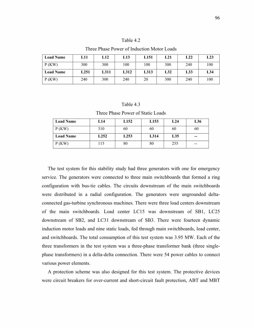
4.2 Three Phase Power of Induction Motor Loads…………………………………..96
4.3 Three Phase Power of Static Loads……………………………………………...96
5.1 Line Impedance…………………………………………………………………111
5.2 Load Power Factors…………………………………………………………….112
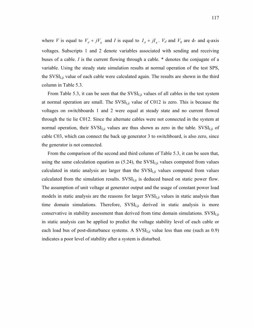
5.3 SVSILji Values of Cables at Normal Operation………………………………...118
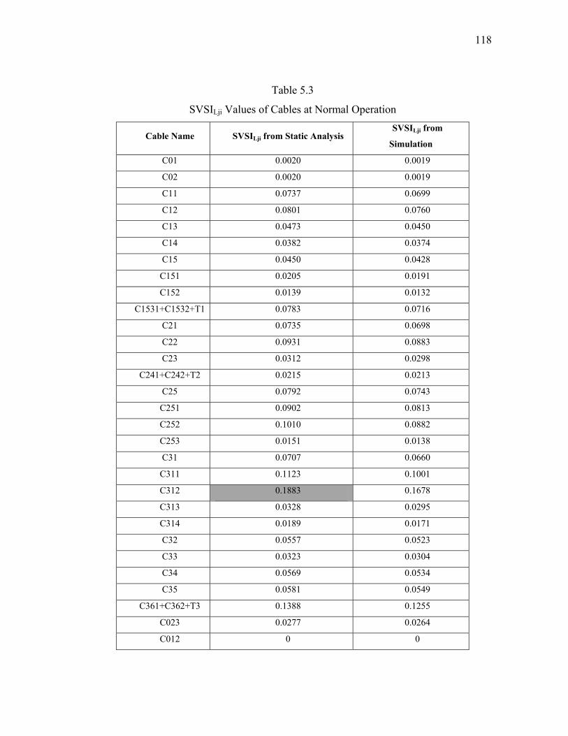
5.4 SVSILji Values of Cables When Loads Are on Alternate Paths………………...120
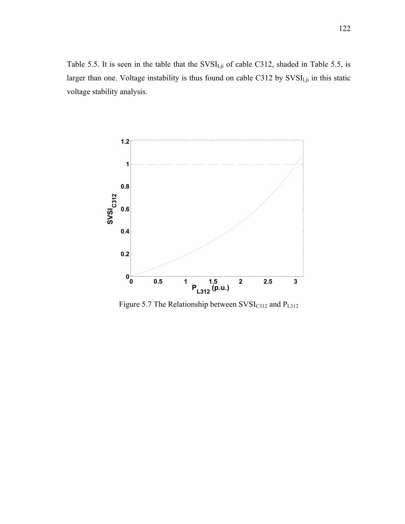
5.5 SVSILji Values When PL312=3.02 p.u…………………………………………...123
6.1 AUTO Results…………………………………………………………………..138
Page 10
x
LIST OF FIGURES
FIGURE Page
3.1 A Typical AC Radial SPS [49] ………..………………………………………..23
3.2 Time Frames for Dynamics of AC Shipboard Power Systems..………………..27
3.3 Illustration of Parallel Operation of Generators in Figure 3.1……..……………34
3.4 Illustration of Saddle Node Bifurcation..………………………………………..42
3.5 PV Curve Analysis for Saddle Node Bifurcation..……………………………...43
3.6 PV Curve Analysis for Losing Equilibrium of Fast Dynamics…..……………..45
3.7 Illustration of Subcritical Hopf Bifurcation..……………………………………47
3.8 Illustration of Supercritical Hopf Bifurcation..………………………………….47
3.9 PV Curve Analysis for Hopf Bifurcation..……………………………………...48
3.10 PV Curve Analysis for Losing Attraction of Fast Dynamics…………………...49
3.11 A Reduced AC Radial SPS……………………………………………………...51
3.12 The Cable between Switchboard 3 and Load Center 2 in Figure 3.11………….52
3.13 PV Curves with Different Load Factors………………………………………...52
3.14 IEEE Type II AVR……………………………………………………………...54
3.15 IEEE Type II AVR with Excitation Limit Reached…………………………….55
3.16 PV Curves With and Without Excitation Limit Reached……………………….57
3.17 Some Typical Torque Speed Curves of Induction Motors……………………...58
3.18 One Line Diagram of a Single-Generator-Single-Load System………………...62
4.1 Transformation Between the Reference Frame dq0 and abc……..……………..73
Page 11
xi
FIGURE Page
4.2 Transformation between Reference Frames…..………………………………...75
4.3 A Three-Phase Connecting Line Model..……………………………………….81
4.4 A Single Phase Linear Transformer Model..……………………………………82
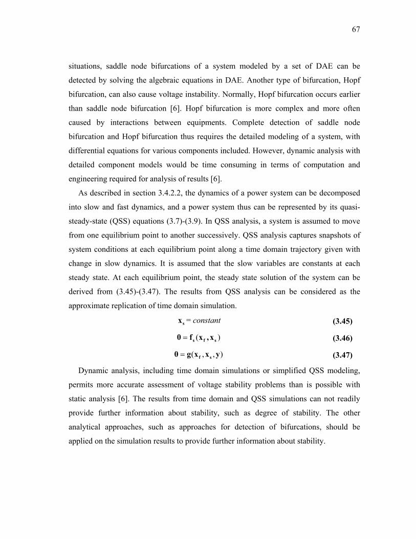
4.5 Interconnection on a Reference Generator Bus…..……………………………..86
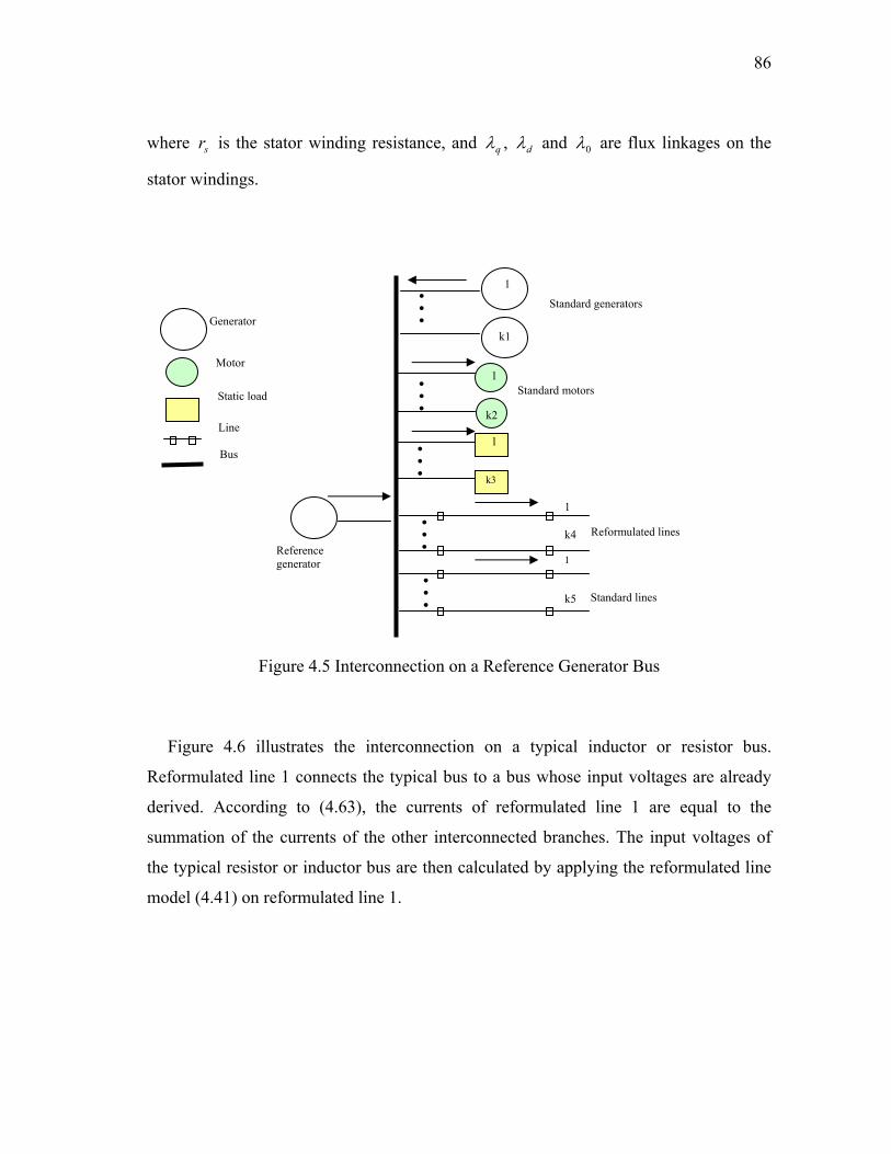
4.6 Interconnection on a Typical Inductor or Resistor Bus…..……………………..87
4.7 A Reduced SPS………..………………………………………………………...88
4.8 Block Diagram of a Governor with Gas Turbine..……………………………...89
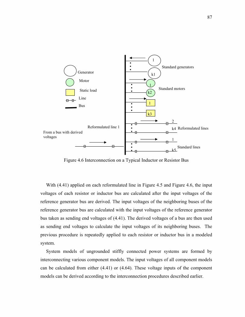
4.9 Phase AB Voltage of Generator 2……..………………………………………..90
4.10 Phase BC Voltage of Generator 2……………………………………………….91
4.11 Phase AB Current of Static Load 5……………………………………………...91
4.12 Phase BC Current of Load 5…………………………………………………….92
4.13 Phase AB Current of Induction Motor 1………………………………………..92
4.14 A Test SPS for Stability Study……………………………………………….....98
4.15 Phase AB Voltage of Generator 1……………………………………………..100
4.16 Phase BC Voltage on Switchboard 3…………………………………………..100
4.17 Phase A Current of Motor Load L11…………………………………………..101
4.18 Rotor Angular Speed of Motor Load L11……………………………………..101
4.19 Phase A Current of Static Load L14…………………………………………...102
5.1 A Two-Bus Power System..……………………………………………………105
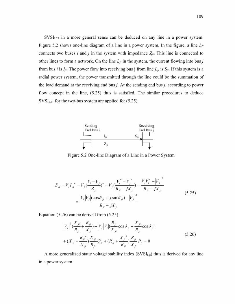
5.2 One-line Diagram of a Line in a Power System..……………………………...109
Page 12
xii
FIGURE Page
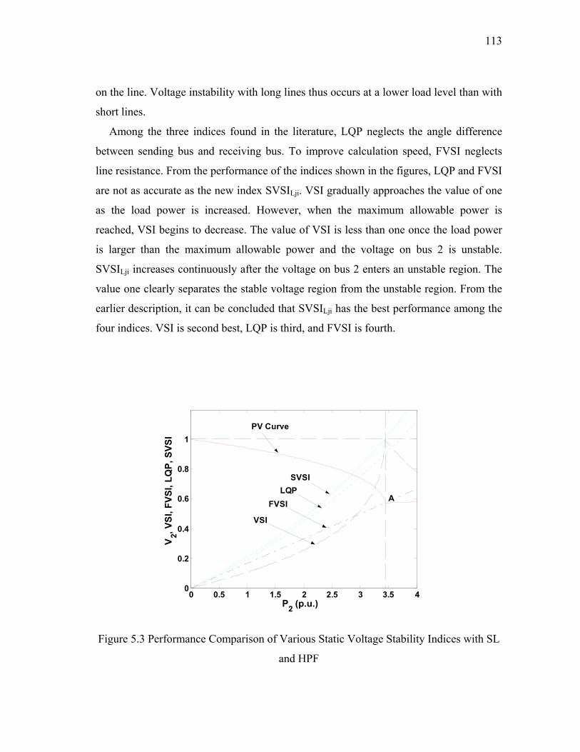
5.3 Performance Comparison of Various Static Voltage Stability Indices with SL and HPF…………………………………………………………………….113
5.4 Performance Comparison of Various Static Voltage Stability Indices with
SL and LPF…………………………………………………………………….114 5.5 Performance Comparison of Various Static Voltage Stability Indices with
LL and HPF……..……………………………………………………………..114 5.6 Performance Comparison of Various Static Voltage Stability Indices with
LL and LPF…………………………………………………………………….115 5.7 The Relationship between SVSIC312 and PL312…..………….…………………122
6.1 A Two-Generator-One-Motor Power System..………………………………..133
6.2 Motor Speed with Change of K……..…………………………………………134
6.3 Voltage on Bus 3 with Change of K……..…………………………………….135
6.4 DVSI with Change of K………..……………………………………………...136
6.5 DVSI1 with Change of K……..……………………………………………….136
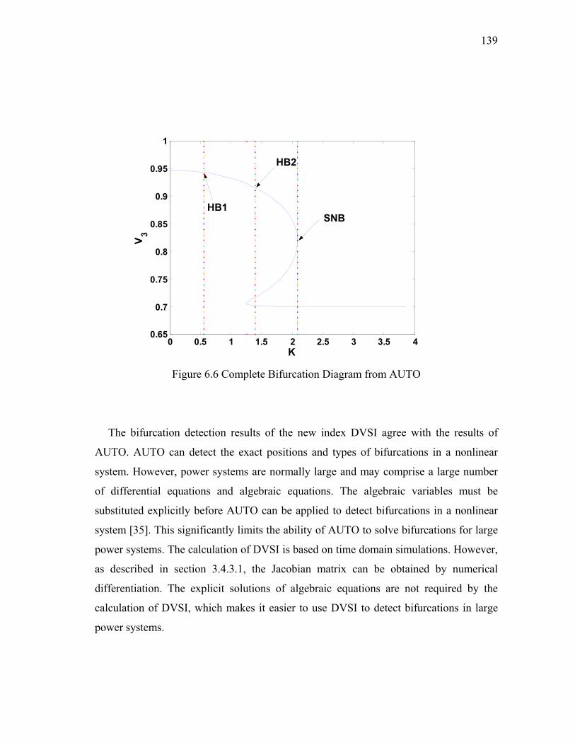
6.6 Complete Bifurcation Diagram from AUTO..………………………………...139
6.7 Root Locus of the Power System in Figure 6.1 for Stability Study…..……….140
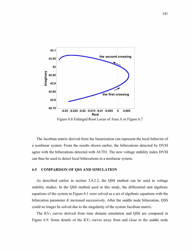
6.8 Enlarged Root Locus of Area A in Figure 6.7……..…………………………..141
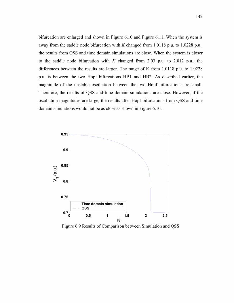
6.9 Results of Comparison between Simulation and QSS…..……………………..142
6.10 Results of Comparison between Simulation and QSS (K=1.0118~1.0228)…...143
6.11 Results of Comparison between Simulation and QSS (K=2.03~2.102)……….143
6.12 Voltage VL312 with Change of K for Various Load Torques………………...147
6.13 Motor Speed WL312 with Change of K for Various Load Torques…………..147
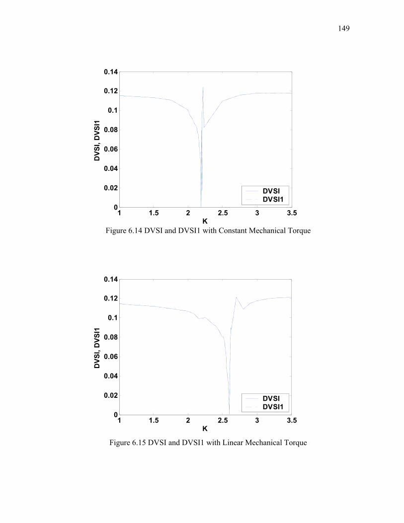
6.14 DVSI and DVSI1 with Constant Mechanical Torque…………………………149
Page 13
xiii
FIGURE Page
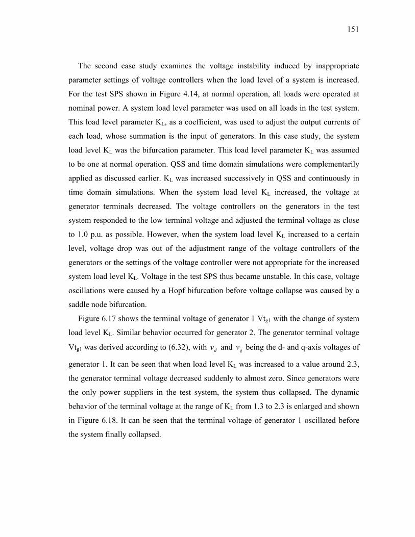
6.15 DVSI and DVSI1 with Linear Mechanical Torque……………………………149
6.16 DVSI and DVSI1 with Quadratic Mechanical Torque………………………...150
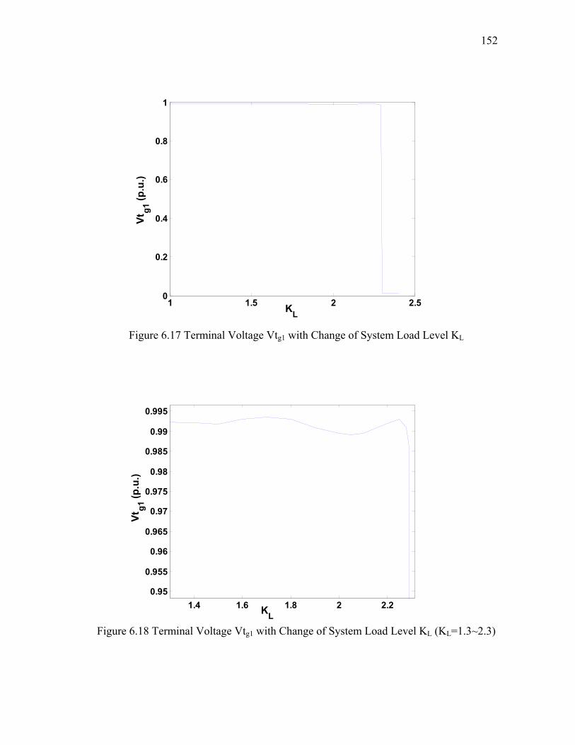
6.17 Terminal Voltage Vtg1 with Change of System Load Level KL……………….152
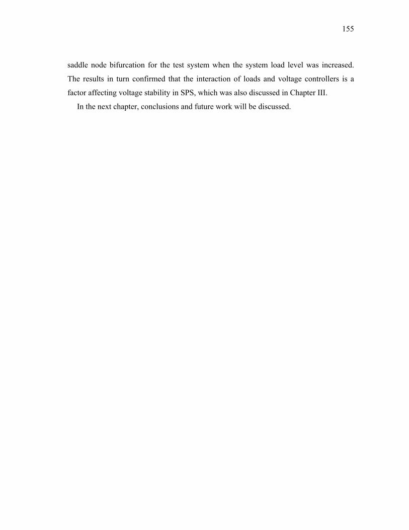
6.18 Terminal Voltage Vtg1 with Change of System Load Level KL (KL=1.3~2.3)..152
6.19 DVSI and DVSI1 with Change of System Load Level KL……………………154
Page 14
1
CHAPTER I
INTRODUCTION
1.1 INTRODUCTION
The electric power systems in U.S. Navy ships supply energy to sophisticated systems
for weapons, communications, navigation, and operation. The reliability and
survivability of a Shipboard Power System (SPS) are critical to the mission of a Navy
ship, especially under battle conditions. In the event of battle, various weapons might
attack a ship. When a weapon hits the ship, it can cause severe damage to the electrical
systems on the ship. This damage can lead to de-energization of critical loads on a ship
that can eventually decrease a ship’s ability to survive the attack. Researchers in the
Power System Automation Laboratory (PSAL) at Texas A&M University have
developed methods for performing reconfiguration of SPS. Reconfiguration operations
change the status of open/close of switches in an SPS. These operations are performed
before or after a weapon hit to reduce the damage to SPS.
Stability is one critical aspect of system reliability, and stable operations must be
maintained during reconfiguration. Power system stability is maintained by real and
reactive power supplied from sources, normally generators. Power systems are stressed
if the margin of real and reactive power between the supply and the consumption is
small. Reconfiguration operations change the topology of an SPS and induce the
dynamics of equipments. When the stability margin is small, the topology changes and
the dynamics of equipments due to reconfiguration might cause voltage instability, such
as progressive voltage fall or voltage oscillations. SPS stability should thus be assessed
to ensure the stable operation of a system during reconfiguration. In the literature, one
methodology is found for angle stability studies for SPS [1], and no methodology was
This dissertation follows the style and format of IEEE Transactions on Power Systems.
Page 15
2
found for voltage stability analysis and assessment for Alternate Current (AC) radial
SPS. Therefore, there is a need to develop new methods that can perform such a task.
To analyze and assess SPS stability, understanding SPS is important and the first
thing to be done. This dissertation presents the time frames of dynamics of SPS. With
appropriate categorization of stability problems due to time frames, we can emphasize
key elements affecting the stability under study. SPS are special power systems, which
have the features of being isolated, ungrounded, and stiffly connected. The salient
features of SPS are discussed. These salient features affect SPS stability and contribute
to the determination of factors involved in SPS stability analysis.
An effective stability assessment methodology can only be developed based on the
study of dynamics during SPS reconfiguration. A “computer model” test system
representing an AC SPS was designed and developed for stability studies. A special
modeling methodology is required to efficiently model and simulate the dynamics of
SPS. Due to the feature of stiff connection, inductor and resistor buses emerge. All
component models on inductor and resistor buses are voltage-in-current-out models and
the voltage inputs can not be derived from any component model, which creates
interconnection incompatibility on inductor or resistor buses. The voltage inputs on
inductor or resistor buses can be generated in artificial ways. In this dissertation, a new
generalized methodology is presented to model and simulate ungrounded stiffly
connected power systems such as SPS. Dynamic simulations are performed on the test
SPS to investigate the dynamic behavior of an SPS during reconfiguration and
simulation results are used in voltage stability and assessment.
Power system stability studies whether a system can regain equilibrium after being
subjected to disturbances. The nature of a stability problem is reflected by synchronism
between synchronous generators or voltages at buses, which belongs to the study areas
of angle stability and voltage stability, respectively. Due to the parallel operations of
generators and the stiff connection of SPS, the synchronism between generators is
strongly maintained in SPS. Hence, voltage stability is the concern of the stability study
in this dissertation. Voltage instability occurs in a stressed system, where reactive power
Page 16
3
margin is small. When a disturbance occurs, voltages in a system can decrease below a
certain level or oscillate. Bifurcations are detected when voltage instability occurs.
In this dissertation, two new voltage stability indices are presented to assess voltage
stability during SPS reconfiguration. The two indices are a static voltage stability index
(SVSILji) for static voltage stability analysis and a dynamic voltage stability index
(DVSI) for dynamic stability analysis. SVSILji and DVSI are used together to assess SPS
stability during reconfiguration. SVSILji is deduced based on the power flow equations at
steady state. In static analysis, instability is detected if SVSILji is equal to one. As the
value of SVSILji gets closer to one, the system is more prone to be unstable. DVSI is
deduced from eigenvalue decomposition and singular value decomposition. DVSI
detects bifurcations in a dynamic system and thus identifies voltage instability. The
dynamic index is evaluated with dynamic simulations, which are performed with the
generalized modeling and simulation method. A zero value of DVSI indicates the
occurrence of bifurcations and voltage instability. The system is prone to be unstable if
DVSI is closer to zero. Case studies were performed for SVSILji and DVSI indices on the
test SPS. Case studies show that SVSILji and DVSI are effective voltage stability indices
in static and dynamic voltage stability analysis.
The major contributions of this dissertation are in six areas. First, the time frames of
dynamic phenomenon were studied for shipboard power systems. The time frames
classify dynamics in SPS into different types of stability. With proper classifications,
stability studies concentrate on important factors affecting SPS stability. Secondly, a
new methodology for modeling and simulating ungrounded stiffly connected power
systems was developed. The obstacles to utilizing conventional power system simulation
methods for ungrounded stiffly connected power systems are discussed. This new
modeling methodology was successfully applied on ungrounded shipboard power
systems. Thirdly, a study of factors affecting shipboard voltage stability during
reconfiguration was conducted and four factors were identified as affecting voltage
stability. The effects of the four factors, loading condition, motor stalling, windup limit
Page 17
4
in voltage controllers, and interaction between loads and voltage controllers on SPS
voltage stability, are discussed and analyzed.
Fourthly, approach to assess SPS stability during reconfiguration was developed. The
approach includes two new indices, SVSILji and DVSI, for static and dynamic voltage
analysis. A new static voltage stability index (SVSILji) was developed. The deduction of
this new index was made from the mathematical formulations of power flows. The
performance of this new index in static voltage stability analysis and assessment was
compared with that of three existing static voltage stability indices found in the
literature. The new index performed better than the three indices. SVSILji was applied on
the test shipboard power system computer model for stability studies. The test system for
stability studies was developed from a reduced shipboard power system model
previously designed in the Power System Automation Lab. The stability studies
performed on the test SPS consider factors affecting SPS stability. A new dynamic
voltage stability index (DVSI) was developed to detect bifurcations in dynamic voltage
stability analysis. Local bifurcations, including both saddle node bifurcation and Hopf
bifurcation, can be detected by the DVSI. The new index was derived with the
techniques of eigenvalue decomposition and singular value decomposition. In a study on
a two-generator-one-motor power system, the bifurcations detected by this new index
agree with those detected on a conventional bifurcation analysis software package called
AUTO. This new index was implemented on the test SPS for stability analysis. The
results show that the bifurcations occurring during dynamic processes of the test system
can be detected by this new DVSI.
1.2 ORGANIZATION
This dissertation consists of seven chapters. In Chapter I, an introduction to this work
and the organization of the dissertation are given. In Chapter II, the literature on stability
studies for conventional utility power systems and shipboard power systems (SPS) will
be reviewed. In Chapter III, stability problems during reconfiguration will be
formulated. This dissertation will discuss stability problems in SPS and study voltage
Page 18
5
stability during SPS reconfiguration. Bifurcations will be introduced as causes of voltage
instability. Steady state and dynamic analysis for voltage stability will be presented as
different ways to analyze voltage instability. Factors affecting voltage stability in SPS
during reconfiguration will be described and analyzed. In Chapter IV, a new generalized
methodology for modeling and simulating ungrounded stiffly power systems will be
presented. A test shipboard power system for stability studies will be constructed in this
chapter. The new modeling and simulating methodology will be implemented on the test
SPS. In Chapter V, a new static voltage stability index (SVSILji) for static stability
analysis will be deduced. Comparisons of the new index and some indices in the
literature will be made. The new SVSILji will be illustrated with the test SPS. In Chapter
VI, a new dynamic voltage stability index (DVSI) for dynamic stability analysis will be
deduced. The bifurcation analysis results of a small power system by DVSI will be
compared with those by AUTO, a conventional bifurcation analysis software. The
effectiveness of the new DVSI will be illustrated on the test SPS. In Chapter VII,
conclusions will be drawn and some remarks about future work will be given.
Page 19
6
CHAPTER II
LITERATURE REVIEW AND BACKGROUND
2.1 INTRODUCTION
In this chapter, the literature on stability and analysis methods will be reviewed and
summarized. Power system stability is an important factor in power system studies.
Shipboard power systems (SPS) are special power systems. Stability analysis and
assessment for AC SPS are the topic of this dissertation.
Appropriate mathematical models of power systems are necessary as the first step for
power system stability analysis and assessment. In this chapter, work on the stability of
utility power systems will be presented first. Work on the stability of SPS will then be
discussed.
2.2 POWER SYSTEM STABILITY
Power System Stability is the ability of an electric power system, for a given initial
operating condition, to regain a state of operating equilibrium after being subjected to a
physical disturbance, with system variables bounded so that system integrity is preserved
[2]. According to the time frames of dynamics, power system stability can be divided
into steady-state, dynamic, or small signal and transient and long-term stability. The
main physical nature of instability in power systems could be angle or voltage.
In this section, modeling work on power systems will be described first. A literature
review of different categories of stability and various analysis methods for utility power
systems will then be presented.
2.2.1 Power System Modeling
Any power system can be represented by a set of differential algebraic equations
(DAE) shown as (2.1) and (2.2) [2].
Page 20
7
),( yxfx =•
(2.1)
),( yxg0 = (2.2)
where ), yx
x is a vector of state variables and describes the dynamics of power systems,
such as the dynamics of exciter control systems. x could also include specific system
configurations and operating conditions, such as loads, generation, voltage setting
points, etc. y is a vector of algebraic variables and satisfies algebraic constraints, such
as power flow equations, which is implicitly assumed to have an instantaneously
converging transient.
The conventional methods for modeling and simulating power systems can be
classified into two main categories: 1) nodal admittance matrix based circuit simulation
methods, such as implemented by EMTP/ATP [3] (The Electromagnetic Transients
Program/Alternative Transient Program), and 2) differential algebraic equation solver
based methods, such as implemented in SimPowerSystems Toolbox by Matlab/Simulink
[4][5]. The essence of nodal admittance matrix based methods is that a power system can
be represented by an electric circuit of mixed constant impedance and voltage source at
each time step. For differential algebraic equation solvers based methods, the differential
equations and algebraic equations are partitioned and solved by explicit numerical
methods or simultaneously solved by implicit numerical methods. Due to the salient
features of SPS, the modeling and simulation of SPS could then be different from the
modeling and simulation of utility power systems, and this will be discussed later.
2.2.2 Steady State Stability
The stability of an electric power system is a property of the system motion around an
equilibrium set, i.e., the initial operating condition [2]. Steady-state analysis consists of
assessing the existence of the steady-state operating points of a power system. At steady
state, time derivatives of state variables are assumed to be zero. Consequently, the
overall DAE equations describing the system are reduced to pure algebraic equations.
No solution for the algebraic equations means that the system cannot operate under
Page 21
8
specific conditions. One solution means that a unique operating point exists. Multiple
solutions means that further investigation is required to study the characteristics of each
solution and find the stable solution. Conventionally, power flow equations are applied
to conduct the steady state analysis. In the past, voltage stability was studied by steady
state analysis methods.
2.2.3 Dynamic Stability
Dynamic stability or small signal stability exists when a system is subjected to small
aperiodic disturbances [2]. The time frame of dynamics in small signal stability is up to
one second. Initially the operating point of a system is ix . After a disturbance, the
operating point moves to ii xx ∆+ , where ix∆ is the deviation of the operating point. In
dynamic stability, the deviation ix∆ is so small that its effects to the system can be
linearized, which is the theory basis for small signal stability analysis. The linear system
depends not only on the physical characteristics of the system but also on the
equilibrium point about which the linearization is performed. The locations of the
eigenvalues of a system are checked for dynamic stability. The imaginary parts of the
eigenvalues represent the potential frequencies of the oscillation modes. The real parts of
the eigenvalues represent the damping factors of the corresponding frequencies. If all the
real parts of the eigenvalues are negative, then the system is stable.
The nonlinear behavior of the system can be approximated by the behavior of its
linear system within a small proximity to the system equilibrium points. The linear
system is almost equivalent to the nonlinear system in a small neighborhood of the
equilibrium point. Within the small neighborhood of the equilibrium point, the
qualitative stability characteristics of the linear system are thus the same as the
qualitative stability characteristics of the nonlinear system. This approximation is the
theoretical basis for the application of local bifurcation analysis for dynamic voltage
stability analysis [6].
Page 22
9
2.2.4 Transient Stability
Transient stability exists when a system is subjected to large aperiodic disturbances
[2]. The time frame of transient stability is up to ten seconds. For transient stability
analysis, the deviation ix∆ of state variables is large and the nonlinear system model can
not be linearized. In the study of power systems, without specification, transient stability
is normally referred to as angle stability. Angle stability is concerned with the ability of
interconnected synchronous machines in a power system to remain in synchronism after
being subjected to a disturbance from a given initial operating condition [2]. The
electromechanical energy conversion in rotating machines is studied for angle stability.
Indirect and direct methods are used in the study of angle stability. Indirect methods
are time domain simulation methods. Time domain simulations compute the solution
trajectories of the state variables from dynamic equations and algebraic equations. The
stability is observed from the solution trajectories. Indirect methods are reliable and
accurate, but the computation results can not indicate the stability margin and the
computation speed is slow for stability assessment [2][7][8].
Direct methods are suggested in many papers for their speed of computation and
efficiency in stability assessment. Good summarization on various direct methods is
made in [7][8]. Basically, Lyapunov functions, usually the energy functions of a system,
are constructed in direct methods to evaluate stability. However, Lyapunov theorem
gives only a sufficient but not a necessary and sufficient condition for the determination
of stability regions. As a result, the stability regions calculated from direct methods are
conservative or smaller than real stability regions. In addition, it is difficult to construct a
Lyapunov function for a system with detailed component models included. Most of the
direct methods are restricted to use with classical second order generator models and
constant impedance load models. In [8], a third order flux decay generator model (a
more detailed generator model) was considered for formulating Lyapunov functions.
Various direct methods use different characteristics of the stability boundary to
determine the stability region. These methods include Unstable equilibrium point (UEP),
controlling UEP, Potential energy boundary surface (PEBS), and Equal area criterion
Page 23
10
(EAC). In the UEP method, the stability boundary is on an unstable equilibrium point
resulting in the lowest value of the Lyapunov function among all the unstable
equilibrium points. In the controlling UEP method, the stability boundary is on a
relevant or controlling unstable equilibrium point or the unstable equilibrium point
closest to the point where the disturbed trajectory exits the stability region. In the PEBS
method, the stability boundary is on the points where the maximum value of the
potential energy occurs along disturbance-on trajectory. The EAC method uses the same
boundary condition as the PEBS method. However, the characteristics of the maximum
potential energy are described in a different way. In EAC, the boundary of the region of
attraction is when the accelerated energy during disturbance-on trajectory is equal to the
decelerated energy after disturbances are removed.
2.2.5 Long-Term Stability
Long-term stability is defined as the ability of a power system to reach an acceptable
state of operating equilibrium following a severe disturbance that may or may not have
resulted in the system being divided into subsystems [2]. Long-term stability problems
are usually concerned with system response to major disturbances that involve
contingencies beyond normal system design criteria. The disturbances are either so
severe or long lasting that they evoke the actions of slow response equipment. Therefore,
long-term stability studies require that the system model include slow response
component models, which are normally considered unnecessary in transient and dynamic
stability studies.
For long-term stability studies, time domain simulations are the only way to evaluate
stability [9]-[11]. In long-term stability studies, different time scales (fast and slow) are
modeled and simulated simultaneously. Long-term stability studies thus could be time
consuming. At present, several specially designed simulation packages, such as
LOTDYS (Long-Term DYnamic Simulation), ETMSP (ExTended Mid-term Simulation
Program) and EUROSTAG (STAlilite Generalisée, in French), can be used to simulate
long-term dynamics. LOTDYS assumes uniform system frequency and neglects fast
Page 24
11
transients [12]. ETMSP is a better simulation program for including fast transients, but it
assumes constant frequency in long-term time frames, which is unacceptable when it is
used for investigating long-term dynamics involving large excursions in system
frequency [13]. EUROSTAG uses the Gear type implicit integration algorithm, in which
time step size varies automatically due to the truncation error of the former step [14]-
[17]. EUROSTAG allows the simulation of all dynamics with one invariant complete
model except for fast electromagnetic transients [14]. In many situations in voltage
stability studies, slow acting equipment will be involved. Long-term voltage stability
could be studied by software packages designed for the study of long-term stability.
The three commercial long-term simulation tools mentioned earlier were developed to
simulate long-term dynamics in bulk power systems, where transmission systems are
significant. If a power system is stiffly connected, due to the small shunt capacitances of
the short lines, the line time constants are small. Therefore, small time steps will be
introduced into the simulation to guarantee a stable integration algorithm even though
the small capacitances have little effect on the overall system performance [18][19]. The
small steps decrease the speed of computation significantly. Consequently, the earlier
mentioned software packages for long-term stability studies are not applicable in stiffly
connected power systems.
2.2.6 Voltage Stability
Voltage stability is the ability of a power system to maintain steady acceptable
voltages at all buses in the system under normal operating conditions and after being
subjected to a disturbance [2]. Voltage stability is not new to the study of power systems
but is now receiving more and more attention as a result of heavier loading in developed
power networks. In recent years, voltage instability has been responsible for several
major network collapses [2]. Voltage instability occurs when a power system is stressed
[2][6][20].
Recently, nonlinear bifurcation theory was applied in a power system voltage stability
study [6]. The bifurcation points are the thresholds where instability occurs. Some
Page 25
12
typical types of bifurcation occurring in power systems are saddle node bifurcation
(SNB), Hopf bifurcation (HB), and singular induced bifurcation (SIB). These
bifurcations are local bifurcations. SNB has been linked to voltage collapse [6]. HB is
associated with oscillatory voltage instability [6]. SNB and HB are generic local
bifurcations [6]. Researchers are unclear as to whether SIB does exist in power systems
or whether it is just a mathematical concept [6].
In voltage stability analysis, load characteristics could be critical. In section 2.2.6.1,
work on loading modeling for voltage stability will be described and discussed. Voltage
stability can be analyzed by static and dynamic analysis methods. In section 2.2.6.2, the
literature on these two analysis methods will be reviewed.
2.2.6.1 Load Modeling
Voltage is maintained by reactive power in power systems. After a system is
subjected to a disturbance, power of loads tries to be restored to the levels before being
disturbed. The restored loads increase reactive power consumption after being disturbed
and can cause voltage instability in stressed power systems. Voltage stability is thus
closely related to load characteristics [2][6][21][22]. The importance of load modeling in
voltage stability studies, especially in the location of the bifurcation points and the
corresponding system dynamic response has been addressed in the literature. Various
load models have been proposed to capture the basic dynamic voltage response of the
loads in a power system.
In [23], the authors examine the characteristics of power systems where induction
motors constitute a main portion of the load. In their study, a first order induction motor
model was used and three different induction motor load models were considered. The
load torques were modeled as constant, linear, and quadratic functions of the induction
motor rotor speed. Static loads were also included in the system model allowing for the
examination of the effect of changing the proportion of the total load, which was
composed of static elements. Fixed voltage and constant generator models were used
with no generator dynamics considered. Different types of load torque on induction
Page 26
13
motors can have different effects on voltage stability. The study found that for constant
load models, saddle node bifurcations occurred at higher voltage levels and at higher
speeds as compared to the speed dependent mechanical load models. The percentage of
the total load composed of induction motor load did not affect the nature of bifurcations,
but it did influence the value of induction motor loading at which the bifurcations
occurred. The effect on voltage collapse of combined induction motor and impedance
loads by means of lab measurements and computer simulations using reduced order load
models is studied in [24]. The study focused on the ability of switching capacitors to
prevent voltage collapse in heavily loaded systems and the operation of induction motors
on the lower portion Power Voltage (PV) curves.
In most voltage stability analysis, studies concentrate on simplified induction motor
models, and little attention has been placed on the interaction of the different power
system components. A Hopf bifurcation was detected along with typical saddle node
bifurcations with a simple two-bus-single-generator system in [25]. The loads in the
system were modeled as a third order induction motor model and lumped impedance
elements. The generator was modeled using a dynamic two axis model with an IEEE
type I exciter. The interaction between the induction motor loads and voltage controllers
on generators was studied in [26]. It was found that the dynamics of induction motors
can delay the response of voltage controllers. Voltage oscillatory instability thus could
be caused by the interaction between voltage controllers and induction motors.
2.2.6.2 Voltage Stability Analysis
At its earlier development stage, voltage stability used to be analyzed by static
analysis methods, such as power flows. However, as understanding of voltage stability
developed, more and more researchers came to believe that voltage stability is dynamic
stability and dynamic analysis should be applied.
Static analysis methods could be used to analyze voltage stability problems
approximately. The equivalence of the occurrence of saddle node bifurcation of the
algebraic equations to the reduced differential equation modeled by a set of DAE is
Page 27
14
shown in [27]. Many static studies have been done on voltage stability in transmission
systems, but hardly any work has been done on voltage stability in distribution systems.
Several voltage stability indices derived from static power flow analysis were proposed
for utility power systems. The values of the indices were calculated for each distribution
line based on load flow results. The line with the largest value was taken as the weakest
line in a system and received special attention to maintain voltage stability. A voltage
stability index LQP that neglected line resistance was proposed by Mohamed [28]. A
fast voltage stability index FVSI was derived in [29] by Musirin. The fast index
neglected the angle difference between the voltages at both ends of a line. A voltage
index was represented by the power injected by the load on a local bus and the power
injected from the other buses in a system in [30]. In [31][32], a voltage stability index
for distribution systems was derived with the whole distribution network represented by
a single line equivalent. However, the equivalent index is only valid at the operating
point at which it is derived and is not adequate for assessing stability when a large
change of load is involved [32].
As described earlier, various long-term simulation packages mentioned in section
2.2.5 could be used for dynamic voltage stability analysis. Voltage magnitudes at critical
buses are observed during simulations to determine if voltages are stable. With
differential equations of fast dynamics approximated by algebraic equations, voltage
stability can be analyzed and assessed by successive static analysis methods, such as
Quasi Steady State (QSS) analysis [2]. In time domain simulations, differential and
algebraic equations are partitioned and solved explicitly, or integrated and solved
implicitly. In QSS, approximated algebraic equations are solved to calculate equilibrium
points successively. Numerical algorithms, such as the Newton-Raphson algorithm, are
applied in QSS for incrementally changing the value of parameters. It has been
suggested that the most effective approach for studying voltage stability is to make
complementary use of QSS and time domain simulations [2][6]. QSS derives the
trajectory approximately. Time domain simulations derive the detailed trajectory
between the equilibrium points derived from QSS analysis when a system is close to
Page 28
15
bifurcations. The bifurcation points can thus be identified along the trajectory by
bifurcation detection techniques, such as eigenvalue decomposition (ED) and singular
value decomposition (SVD) [6]. The minimum singular value can be used to detect
bifurcations for voltage collapse [6]. However, in a real power system, several small
singular values could mask the critical singular value, and a method is suggested in [33]
to unmask the critical singular value. In many long-term stability studies, successive
static analysis is thus applied for determining long-term stability margins and identifying
factors influencing long-term stability [2][6][34]. However, numerical difficulties can
arise as the solution of steady state equations approaches a singular point caused by
saddle node bifurcation.
Continuation methods overcome the singular problem by reformulating the
differential algebraic equations so that they will remain well-conditioned at all possible
loading conditions. Continuation techniques are generally composed of two or three
steps. The first step is a predictor step, the second is a corrector step, and the last step is
a parameterization routine. At the predictor step, a predictor step of state variables and
the change of parameters are determined. From the new point, a corrector routine is used
to calculate the new equilibrium point. A parameterization is used to ensure that the
Jacobian matrix used in the continuation method does not become singular at saddle
node bifurcations. UWPFLOW, a publicly available QSS, uses a continuation method to
detect the voltage stability limit of a power system [34]. Another public program AUTO
[35] is also mentioned in the literature. AUTO applies a continuation method to solve the
differential algebraic equations of the system. AUTO has been used for theoretical
studies of bifurcations in small power systems [6][36].
2.3 SHIPBOARD POWER SYSTEM STABILITY
The stability analysis for SPS is different from stability analysis for conventional
utility power systems. Little research work has been found in the literature in the area of
shipboard power system stability.
Page 29
16
In this section, shipboard power system modeling will first be reviewed. Secondly, a
method found in the literature for SPS stability analysis and assessment will be
discussed.
2.3.1 Shipboard Power System Modeling
Shipboard power systems are isolated finite inertia power systems. References [37]-
[43] presented modeling and simulation studies of versatile isolated finite inertia power
systems from different perspectives. Ross, Concordia and O’Sullivan [37]-[39] modeled
isolated power systems for designing frequency controllers. Kariniotakis and Stavrakakis
[40] neglected machine stator transients and network transients. Their methods thus
derived incorrect simulation results when the transients were large. The objective of
Sharma [41] was to consider transients in the first five seconds, so detailed models were
not applied. Fahmi and Johnson [42] divided an isolated power system into several
subsystems, with phase co-ordinate models then adopted for analysis of each subsystem.
Limited controller models were included, which would not be appropriate in long-term
stability studies. Murray, Graham and Halsall [43] concentrated on the modeling of
synchronous motor drives and the simulation of waveform distortion due to motor drives
in an isolated power system.
A test ungrounded delta connected SPS was developed in the Power System
Automation Lab based on a U.S. Navy combatant ship [44]. The modeling and
simulations of the test SPS were conducted with Alternative Transient Program (ATP).
The test SPS comprised various components, including generators, load centers,
numerous cables, induction motor loads, constant impedance loads, transformers, and
different types of protective devices. The test SPS provided a platform for studying the
behavior of SPS. The test system was simulated to aid the development of automated
failure assessment and restoration for SPS.
With small shunt capacitance neglected in SPS, there emerges incompatibility when
the components models are interconnected. The incompatibility problem caused by
neglecting the capacitances in modeling SPS could be solved by the traditional method
Page 30
17
of adding auxiliary resistance in systems [8]. Two methods for modeling and simulating
SPS were proposed in [18][19] to solve the modeling incompatibility. In [18], at each
inductor bus one component model is reformulated. The reformulated component is a
nonroot generator or motor. The original physical models of the reformulated
components are kept, while reformulation changes the mathematical formulation of the
reformulated component models to facilitate the derivation of bus voltages. The method
in [19] keeps the original mathematical format of equations and derived bus voltages by
solving algebraic constraints with an algebraic solver; as a result, the speed of
computation improved greatly.
The methods in [18] and [19] used ACSL (Advanced Continuous Simulation
Language) as the simulation tool. In Mayer’s method [18], the inductor buses in a stiffly
connected system are first categorized; the standard model of one machine connected to
each inductor bus is then reformulated to facilitate the deduction of the inductor bus
voltages. Mayer’s method requires that at least one machine be connected to each
inductor bus and certain procedures are required to solve the voltages of each inductor
bus on the basis of the reformulated state space equations of root and nonroot machines.
Ciezki’s method [19] relies greatly on the simulation language, more specifically, the
accuracy of the algebraic solver in ACSL.
2.3.2 Shipboard Power System Stability Analysis
A stability analysis and assessment method for composite systems was discussed and
proposed for SPS by Amy [1]. A composite system was modeled as (2.3) and (2.4) [1].
iiiii uDtxfx +=•
),( (2.3)
iii xHy = (2.4)
where ix is the states of the ith subsystem, iu is the inputs of the ith subsystem, and iy
represents the outputs of the ith subsystem. iG and iH are system parameters. The
representation of interconnection of subsystems was given by (2.5) [1].
Page 31
18
∑=
+=m
jiiiji uGyBu
1 (2.5)
where ijB describes the interconnections between the inputs of ith subsystem and the
outputs of the other subsystems. u is the global inputs to the composite system. G
represents the parameters associated with the global inputs. A Lyapunov function was
constructed from the composite model (2.3)- (2.5) to assess system stability [1].
Amy considered SPS as a composite system, and each component was taken as a
subsystem in the composite system [1]. However, the close proximity and tight coupling
of SPS components increase the order of models to capture dynamics. Further, it was
difficult to construct a Lyapunov function for a detailed system model. Co-energy was
used by Amy to construct Lyapunov functions for detailed generator models in SPS [1].
He assumed each generator was a lossless “coupling field” where the mechanical and
electrical interaction takes place. The energy contained within the “coupling field” was
co-energy. Amy then used the instantaneous co-energy stored in a generator and its rate
of change for stability analysis and assessment during the transient process [1]. At steady
state, the co-energy was stationary and the mechanical energy injected into the field was
extracted as electric power. Co-energy within the field did not directly participate in
electromechanical energy conversion at steady state. When the system was disturbed, co-
energy in generators increased. After the disturbance, if the excess co-energy stored in
the coupling field was extracted and converted into the electrical system, the system was
stable. Otherwise, the system was unstable.
Co-energy in a three-phase synchronous machine in dq0 variables was written as
(2.6) by Amy in [1].
[ ]
=
R
dqDQ
TT
II
LIIWRdqmdq 2
1' (2.6)
where dqI is the stator currents and RI is the rotor currents. DQL is the stator and rotor
inductance of the generator. A co-energy based Lyapunov function including kinetic
energy K.E. as (2.7) was then developed by Amy for detailed SPS generator models [1].
Page 32
19
[ ] 2''
21
21..
mRdqmdqmJ
II
LIIEKWVR
dqDQ
TT ω+
=+=
(2.7)
where J and ω are the inertia and rotor speed of the generator. Four other Lyapunov
functions with different scaling factors on co-energy and kinetic energy were also
presented [1]. Since a SPS is a composite system, Amy used the summation of the
Lyapunov function of each individual generator as the system Lyapunov function of a
SPS [1]. If the derivative of the system Lyapunov was positive, then the system was
determined unstable. Otherwise, the system was determined as stable. The co-energy
based Lyapunov function was applied by Amy to analyze stability of a simple two-
generator SPS [1]. In the system, one generator was a super-conducting generator and
the other was a conventional generator. A short circuit fault was applied at the terminal
of the super-conducting generator. The critical clearing time for the faults was
determined as the time instant when the derivative of the system Lyapunov was equal to
zero.
The concept of a co-energy based Lyapunov function needs some improvement to be
feasible in real SPS. In order to assess system stability, Amy believed each relevant
component in a system should have its own “co-energy based” Lyapunov function [1].
However, the implementation of the co-energy concept on components other than
synchronous generators needs further research work. In addition, because the co-energy
in generators is normally small, weighting factors were used by him to enlarge the co-
energy in the total energy [1]. These weighting factors are important for assessing
stability accurately. An efficient way to select the weighting factors is necessary for the
co-energy based Lyapunov function to be used in stability analysis.
2.4 CHAPTER SUMMARY
This chapter addressed the literature on stability. Stability and its analysis methods
for conventional utility power systems were presented. Different methods of modeling
and simulations of SPS were reviewed. A stability study method developed for
shipboard power systems was described and discussed.
Page 33
20
Chapter III will formulate the stability problems studied in this dissertation.
Page 34
21
CHAPTER III
PROBLEM FORMULATION
3.1 INTRODUCTION
The electric power systems in U.S. Navy ships supply energy to sophisticated systems
for weapons, communications, navigation and operation. At present, there are many
forms of system configuration for electric power systems in U.S. Navy ships or SPS,
such as AC radial, AC zonal, and integrated power systems (IPS) [45]-[47]. Some AC
shipboard power systems (SPS) are ungrounded, having no permanent, low-resistant
connections between the power system and the structure of the ship [45]. An ungrounded
power system is used for AC radial SPS to survive the most frequently occurring single-
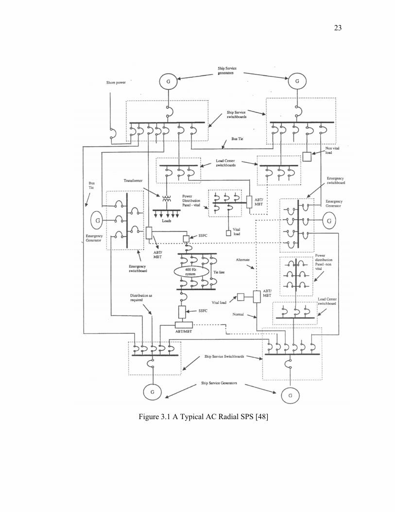
line-to-hull fault. Figure 3.1 shows the one-line diagram of a typical AC radial SPS [48].
In SPS, some generators are in normal operation, and some are back-up or standby
generators that provide generation in emergencies. In Figure 3.1, four generators are in
service and two are emergency generators that provide back up power. Typical voltage
output from the generators is 450 volts AC at 60 Hz. To further enhance survivability of
an SPS under attack, main switchboards are connected with bus-tie cables in a ring
configuration. In emergencies, the ring connection provides power supply from the
generators to the main switchboards through alternate paths. To avoid total generation
loss under attack, the generators are located in different places on shipboard.
Circuits downstream of the main switchboards are in radial configuration. The load
centers are downstream of the main switchboards; while the power panels are
downstream of the main switchboards or load centers. Loads directly connect to the
main switchboards, load centers, or power panels. Single-phase loads connect to power
panels through power transformers. Transformer banks are three, single-phase delta
connected transformers that reduce the voltage to supply single-phase loads.
Transformers convert the supply voltage of the distribution system from 450 volts to 120
volts. Therefore, an SPS could operate under unbalanced conditions. Loads operate at
Page 35
22
440 or 115 volts at 60 Hz or 400 Hz. 400 Hz loads are usually part of the weapons
systems and aircraft and aviation equipment.
Generally, generators, main switchboards, and load center feeders are equipped with
circuit breakers (CBs), while power panel feeders are equipped with switches or fuses
[45]. Switchboard protection devices, including an under-frequency module relay, an
over-power relay, a reverse power relay, and an under-voltage relay protect its
associated generator/switchboard set [49]. Low voltage protective devices (LVs), such as
low voltage protection (LVP) and low voltage release (LVR), are installed to protect
induction motors. LVPs and LVRs isolate the protected motor if the terminal voltage is
below the drop out voltage. If the terminal voltage is restored to a value above the pick
up voltage, the LVR switches the load back into the system. LVPs require manual
operator action to switch the load back into the system.
There are two categories of loads in the system: non-vital loads and vital loads. Non-
vital loads have one path (normal path) to achieve power supply; while vital loads have
an extra path (alternate path) to enhance survivability in emergencies. Two kinds of bus
transfer units (BTs), automatic bus transfer (ABT) units and manual bus transfer (MBT)
units, are employed to perform this protection function. The switches of a bus transfer
unit on the normal path of the load are normally closed, while the switches on the
alternate path are normally open. An ABT automatically switches the load to its alternate
path if the voltage on the normal path is below the drop out voltage, and returns to its
normal path when the voltage returns to a value above the pick up voltage. An MBT
needs manual interaction to change the path of the protected load.
Page 36
23
Figure 3.1 A Typical AC Radial SPS [48]
Page 37
24
The reconfiguration phenomenon in SPS is divided into three types. They are static
reconfiguration, mission reconfiguration, and dynamic reconfiguration. Static
reconfiguration implies the choosing of the actual shipboard power architecture but also
includes platform performance upgrades by means of software and open architecture
based upgrades [50]. Mission reconfiguration means a change in platform state in
response to varying readiness conditions such as cruise, on-station, anchor, battle, etc
[50]. Dynamic reconfiguration is a platform response to assure electric power to vital
loads during damage or failure [50]. Dynamic reconfiguration commonly occurs during
rapidly changing conditions such as battle. Dynamic reconfiguration is the type of
reconfiguration that was studied in this dissertation.
In the event of battle, various weapons might attack the ship. When a weapon hits a
ship, it can cause damage to the electrical system on the ship. The effects of damage to
the SPS comprise open and short circuits from damage to equipment [48]. Two types of
dynamic reconfiguration are being studied by researchers in the Power System
Automation Lab (PSAL). They are restorative reconfiguration and predicative
reconfiguration. Reconfiguration operations change the open/closing status of circuit
breakers, bus transfers, and low voltage protective devices. The multiple closing/opening
of switches and protective devices changes system configuration and reduces the system
loss caused by damage.
For power systems, the process of a system being disturbed can be subdivided into
three stages: pre-disturbance, disturbed, and post-disturbance [2]. A power system is
initially operating at an operating point. After being subjected to disturbances, the
system could regain or lose a state of operating equilibrium. For dynamic
reconfiguration of SPS, disturbances include the effects of damage, such as open circuits
and short circuits, and reconfiguration operations. The pre-disturbance stage during SPS
reconfiguration is up to the instant when the first disturbance occurs. The post-
disturbance stage during SPS reconfiguration is from the instant when the last
disturbance occurs. The disturbed stage during SPS reconfiguration is the transient
process after the pre-disturbance stage and before the post-disturbance stage.
Page 38
25
Stability is an important condition for the success of reconfiguration. During SPS
reconfiguration, an SPS starts from steady state at the pre-disturbance stage, experiences
the transient process at the disturbed stage and finally settles down to steady state at
post-disturbance stage. Stability during reconfiguration studies if a SPS will settle down
to a state of operating equilibrium at the post-disturbance stage. If instability occurs
during reconfiguration, a SPS would move to some unknown state. Instability is
undesirable during the operation of a SPS. Therefore, SPS stability should be analyzed
and assessed before any reconfiguration operation is undertaken.
In this section, shipboard power systems and reconfiguration are introduced. This
dissertation concentrates on stability during dynamic reconfiguration. The complexity of
a system model and analysis methods for stability studies depends on the type of a
stability problem and the characteristics of the system studied. In section 3.2, SPS
dynamics will be categorized according to the results of time frame analysis. In section
3.3, some salient features of SPS will be presented. The effects of the features on
stability will be discussed. Based on the classification of SPS dynamics and the features
of SPS, the stability problems during SPS reconfiguration will be formulated in section
3.4. Two types of stability issues in SPS, angle stability and voltage stability, will be
analyzed. Voltage stability problems will be shown to be the main stability problems.
Four factors affecting voltage stability during reconfiguration in SPS will be analyzed.
Static and dynamic analysis can be applied for voltage stability analysis. Considering
static or dynamic effect on voltage stability, the four factors affecting voltage stability
can be analyzed in static or dynamic analysis.
3.2 TIME FRAME ANALYSIS OF SPS DYNAMICS
With appropriate categorization of stability problems, we can emphasize key elements
that affect stability studies. Time spans or time frames of dynamics can be used to
classify stability problems. Time frames of power system stability problems for
conventional utility power systems are given in and [51]. Detailed time frames of
voltage stability problems for conventional utility power systems can be found in [20].
Page 39
26
Classifications of stability problems for conventional systems can be found in [2]. The
larger a disturbance, the longer the duration of the dynamics due to the disturbance. Due
to different time frames, stability problems can be classified into small signal or dynamic
stability, transient stability, or long-term stability. Small signal and transient stability can
be grouped under short-term stability [2]. The time frame of small signal stability or
dynamic stability is up to one second, the time frame of transient stability is from one to
ten seconds, and the time frame of long-term stability is from ten seconds to tens of
minutes.
Figure 3.2 shows the time frames of relevant dynamics in AC SPS. Electronic
transients are defined as the sudden turn-ons of an electronic type load such as radar high
voltage direct current power supplies or the sudden turn-offs of a radar system by its
protective device [52]. Military specification requires that the voltage at the terminals of
the electronic loads recover and stay within the steady state regulation band within 0.02
second after application of the loads. In the design of a future generation of shipboard
power system PEBB (Power Electronic Building Blocks), it is suggested that switching
frequencies of Pulse Width Modulator (PWM) used for a wide range of inverter and
rectifier applications reduces as power rating of the associated load increases [53]. The
switching frequencies should be 200HZ, 2KHZ, and 20KHZ with different power
ratings. The time frame of switching surges of PWM is from 0.005s to 50us. The
stability of transients of electronic loads and switching surges thus belongs to dynamic
stability. The time frames of the dynamics caused by machines, fast controllers,
protective devices, faults and generator removal last no more than ten seconds. The
corresponding stability problems thus fall into the categories of dynamic and transient
stability. The time frames of the dynamics caused by slow controllers, nonlinear limits,
load shedding and incremental loading for restoration could be several minutes. The time
frames of load increasing on ships are in a ship’s lifetime. The stability of dynamics
caused by load shedding, incremental loading for restoration, slow controllers, nonlinear
excitation limits, and load increasing thus belongs to long-term stability.
Page 40
27
Figure 3.2 Time Frames for Dynamics of AC Shipboard Power Systems
Time constants of stators and rotors of machines in SPS, including generators and
induction motors, determine the time frames of machine dynamics. Similarly, time
constants of controllers in SPS determine the time frames due to controller dynamics.
The response of some controllers in SPS, such as governors and automatic voltage
regulators (AVR) take several seconds. These controllers are fast controllers. The
response of some other controllers in SPS, such as prime movers, including boilers and
switching surges
10-5 10-3 0.1 10 103 10510-7 Time (seconds)
subsynchronous resonance, stator transients
electronic transient
governor, voltage regulator, induction motor dynamics
boiler, gas turbine, steam turbine start-up, over load protection
10-5 10-3 0.1 1 10 103 10510-7
1.0s 10.0s
Dynamic stability Transient stability Long-term stability
load shedding, incremental loading
generator removal, system faults, CB, LVP/LVR, BT, under frequency, under voltage, and reverse power relays
Load increase
Excitation limiting
Page 41
28
gas turbines, could normally take several minutes. These controllers are slow controllers.
If a voltage controller has nonlinear excitation limits, the response of the limits may take
several minutes or even longer.
The response time of protective devices in SPS, including CBs, LVs and BTs,
determine the time frames of dynamics caused by protective devices. To derive the time
frame of these dynamics, a two-generator system was modeled. The two generators were
connected by one line. Simplified component models for generators and lines were then
used for the analysis for faults and generator removal. Response time curves for faults
given in [54] were applied to derive the time frames of line-to-line faults, double line-to-
ground faults, and three-phase ground faults, respectively. Response time curves for
generator removal given in [54] were used to obtain the time frame of generator
removal.
The process of some operations determines the time frame of the dynamics caused by
these operations. Load shedding in SPS due to overloaded generators can be divided into
several stages. It may take several minutes to complete the whole process.
Reconfiguration operations for restoration bring de-energized loads back on line. The
incremental loading due to restoration could last for minutes or hours. On a Navy ship,
the load profile increases continuously over a ship’s lifetime. Historically, loading could
increase twenty percent during the lifetime of a ship [1].
Comparing the time frames given in [2] and [20], most SPS dynamics have the same
time frames as utility power systems. However, the time frame of subsynchronous
resonance of SPS is different from that of utility power systems. To determine the time
frame for subsynchronous resonance, a one-generator system was modeled. The
simplified mechanical and electrical systems of the generator in the system were used.
The frequency range of subsynchronous resonance of SPS was derived following the
approaches in [55]-[58]. Due to the low inertia of generators in SPS, the derived
frequency range of SPS was smaller than the frequency range of utility power systems.
Therefore, the time frame of subsynchronous resonance in SPS is longer than that in
utility power systems.
Page 42
29
Reconfiguration comprises a set of control actions to change the system configuration
and transfer loads. Reconfiguration operations could cause dynamics in SPS, such as the
dynamics of generators, loads, controllers, and protective devices. As seen in Figure 3.2,
these dynamics occurring during reconfiguration could fall within the areas of dynamic
stability, or transient stability. During dynamic reconfiguration, SPS may need to
respond to major disturbances, such as a hit by weapons. Under this condition, the slow
dynamics of equipment in SPS, such as start up of generators, may be taken into
consideration. Some reconfiguration, such as reconfiguration for restoration, could be
undertaken in several stages. The corresponding reconfiguration operations are thus
taken sequentially in the long-term. Consequently, the time frames of individual
dynamics involved in reconfiguration could be short-term (including dynamic or
transient periods). However, considering the longest possible dynamic response during
the process of reconfiguration, the stability study during reconfiguration thus falls into
the category of long-term stability. The stability study occurring during reconfiguration
extends beyond the time frame of transient stability to include, in addition to fast
dynamics in short-term periods, the effects of slow dynamics in the long-term.
3.3 SPS SALIENT FEATURES
SPS are special power systems. Generally, an SPS is a small isolated or island electric
power system, relatively small and isolated from neighboring power systems electrically.
Features of isolated and island power systems can be found in studies [1][37][43]-
[48][59]-[62]. Some salient features of SPS and their effects on SPS stability studies are
discussed as follows:
--- The generation of SPS has limited capacity and inertia, and lacks support from
neighboring power systems. Being small and isolated from other power systems makes
SPS susceptible to disturbances. Deviations of bus voltages and system frequency from
nominal values due to disturbances could be large.
Due to this feature, some common sense experience used in utility power system
stability analysis would not apply in SPS. In utility power systems, the inertia of a
Page 43
30
critical generator is much smaller than the total inertia of the rest of the machines of the
system. An infinite bus thus is able to represent the rest of the system in angle stability
analysis. The number of machines in SPS is limited. The finite inertia amount of one
generator is comparable to the total inertia of the other machines in SPS. Thereby, the
concept of infinite bus is not applicable for SPS stability analysis.
--- Connecting cables are short in length and transmission is thus not as significant as
for utility power systems. Shunt capacitance on cables is small. Cables thus have small
electrical time constants, and electrical transients on cables are short. Due to the short
cable, the electric transients on networks of SPS are very short and can be neglected
[18]. Due to the short connecting cables between components, SPS is tightly coupled. The
generators on ships are strongly synchronized. Due to the tight coupling, interactions
between types of equipments (for example, interactions between controllers and
induction motors) are strong. The strong interactions would affect controller dynamics
and may even cause instability. To observe complete interactions in such a tightly
connected power system, detailed component models should be employed in SPS
stability analysis.
--- Induction motors are predominant in SPS. In utility power systems, motors take
approximately fifty-seven percent of consumed power, and ninety percent of motors are
induction motors [20]. On ships, induction motors make up approximately seventy–
eighty percent of total loads [1]. In SPS, it is possible that generators may be connected
to several paralleled large induction motors. With a large amount of induction motors
loads, SPS stability analysis and assessment require careful consideration of the
characteristics of induction motors.
Induction motors increase nonlinearity in system models and could have adverse
effects on controller dynamics. The response speeds of induction motors, determined by
a motor’s inertia and rotor flux time constant, are comparable to the speed of response of
voltage controllers. The motor dynamics may thus affect the functions of voltage
controllers adversely. For example, the negative damping of induction motors may
Page 44
31
induce unstable oscillatory voltage stability in power systems [26]. In such a tightly
coupled system as SPS, the interactions between motors and controllers are thus greater.
Higher order models of induction motors may be required to determine the detailed
effects of dynamic loads on SPS stability.
If the load torque of a motor exceeds the electrical torque, the motor decelerates. If
the load torque exceeds the maximum electrical torque of a motor, the motor could stall
or become unstable. Motor instability belongs to the study of voltage instability
[2][6][20]. In SPS, due to the small inertia, the speed reduction of motors is large. The
greatly reduced motor speed would impose large, low power factor “starting currents” on
the network after the causes of deceleration are removed and motors reaccelerate. The
more motor speeds are reduced, the larger the reaccelerating currents. The reaccelerating
currents are the largest when Black Start starts to occur. If the network is not strong
enough to reaccelerate the motors, system voltage would be depressed and motor speeds
would continue to decay. The large amount of current drawn by stalled motors would
reduce system voltage even further and cause motor stalling elsewhere in the system,
thereby giving rise to cascaded motor stalling [63][64]. The stalling of large induction
motors and cascaded motor stalling may induce system wide voltage collapse.
--- An SPS has fast controllers to maintain system frequency and voltage. The fast
controllers could pull voltages and frequency in a disturbed system back within the
allowable ranges quickly. For fast controllers, the overshoot of a controller would be
sacrificed to achieve the prompt control. In SPS, negative damping generated by fast
response controllers could cause oscillatory instability.
Basically, an SPS is a system susceptible to disturbances and includes a predominant
number of induction motor loads. The salient features of SPS should be considered for
modeling SPS appropriately. These salient features are important for the stability
analysis and assessment of AC SPS.
Page 45
32
3.4 STABILITY ISSUES IN SPS
According to the physical nature of stability problems, they belong to two types:
angle stability and voltage stability. In this section, both of these types of stability
problems will be discussed as they apply to AC SPS.
3.4.1 Angle Stability
Angle stability is the ability of a power system to maintain synchronism when
subjected to disturbances [2]. If the angular separation between the synchronous
generators in a system remains within certain bounds, the system maintains
synchronism. Any instability that may result occurs in the form of increasing angular
swings of some generators, leading to their loss of synchronism with other generators.
The angle stability problem is one of holding disturbed generators in synchronism with
the remaining generators.
Angle stability studies the electromechanical oscillations inherent in power systems.
The electromechanical equation of a synchronous generator can be described by (3.1).
)(21
2
2
EM PPHdt
d−=
δ (3.1)
where δ is the rotor angle, ω is rotor speed. MP is the mechanical power, and EP is the
electrical power. H is the inertia constant. The electrical power EP is a function of bus
voltages and admittance between buses. Based on (3.1), for a power system having two
finite generators, the angle difference between the two finite generators could be solved
by (3.2) [65]. Subscripts 1 and 2 indicate variables associated with generators 1 and 2.
21
2112
21
2112212
2
21
21
HHPHPH
HHPHPH
dtd
HHHH EEMM
+−
−+−
=+
δ (3.2)
2112 δδδ −= (3.3)
The mechanical power of each generator is determined by the load assigned to the
generator and normally assumed to be constant during a transient angle stability study.
When a generator is disturbed, the electrical power would increase or decrease, and the
Page 46
33
generator would decelerate or accelerate correspondingly. The angle difference between
accelerating generators and decelerating generators could increase. If the angle
difference is over a certain limit, the system becomes unstable. From (3.1), it can be seen
that angle stability is the ability to maintain or restore equilibrium between
electromagnetic torque and mechanical torque of each synchronous generator in a
system.
All ship designs are provided with multiple ship service generators, designed to be
operated either in split or parallel modes. Parallel operation is emphasized during normal
operation to provide for continuity of power while minimizing the magnitude of system
voltage and frequency variations [45]. Split operation is used when maximum reliability
of ship service power is required and is normally used during battle conditions to avoid
cascading failures of the entire electric plant [45]. Split plant operation has generators
operating independently, with each generator serving different groups of electrical loads
[45]. Since generators operate independently in split operation, angle stability is only of
concern for generators in parallel operation. Angle stability studies the synchronism
between multiple generators. Parallel operation of the AC generators in Figure 3.1 is
illustrated in Figure 3.3. The generators are considered to be paralleled by the associated
switchboards.
Page 47
34
Figure 3.3 Illustration of Parallel Operation of Generators in Figure 3.1
As described earlier, the generators of SPS have finite inertia. An SPS with two
generators can thus be analyzed by (3.2). From (3.2), it can be seen that the mechanical
and electrical power determines the angle difference between generators. For generators
in SPS, governors are installed to adjust steam or fuel to prime movers. Using governors,
paralleled generators divide the total load between the various units installed according
to the capacities of the generators [65]. Generators in SPS are designed to have the same
capacity. Loads are thus divided equally between the generators. Due to the equal load
sharing in SPS, the mechanical power of the paralleled generators is equal. (3.2) thus can
be rewritten as (3.4). Constant H represents the same inertia of the two finite
generators.
)(21
21212
2
EE PPHdt
d−−=
δ (3.4)
As described earlier, the electrical power of a generator is the function of the voltage
at buses and admittance between buses. The generators are considered to be paralleled at
their switchboards and thus have the same terminal voltages. Due to limited space, the
Switchboard
G
G
G
G
G G
Page 48
35
lengths of cables between buses to the paralleled generators are of the same order of
magnitude. Any disturbance downstream in the generator switchboards affects each
generator almost equally. Therefore, the electrical power difference 21 EE PP − in (3.4) is
very small.
Power tending to bring the generators into synchronism is termed synchronizing
power. If generators operating in parallel get out of synchronism, there is a circulating
current between the paralleled generators. The circulating current flows between the
armatures of the paralleled generators. Because the armature reactance of generators is
larger than the armature resistance, the circulating current is in phase with the leading or
accelerating generators. The leading generators then pump electrical power into the
lagging generators. The accelerating generators tend to slow down while the decelerating
generators tend to speed up. The circulating current thus tends to pull the out of
synchronism generators in parallel operation back into synchronism. It is concluded that
the synchronizing power between paralleled generators is strong [66]. The disturbances
in SPS thus have little tendency to make the paralleled generators lose synchronism.
From the analysis earlier, it was found that the most severe disturbances from the
standpoint of angle stability analysis are the disturbances that make load distribution
unevenly or occur closely to one generator. In SPS, load distributions are even between
generators, and any disturbance downstream of the generator switchboards has similar
closeness to the generators. Angle stability of SPS then could be affected by relatively
more severe disturbances, such as short circuits upstream of the generators. However,
when the disturbance occurs at the terminal of a generator, the voltage and frequency
excursions of generators in SPS are large. In SPS, large excursion of voltage and
frequency could trip the breakers on switchboards and split generators. For example, the
Synch Monitor would prevent the paralleling of generators unless the frequency
deviation is less than two percent, the voltage deviation is less than five percent, and the
angle difference is less than 30 degrees [49]. The system would go into split operation
before it becomes unstable.
Page 49
36
In summary, synchronism between generators in tightly coupled SPS is strong. The
synchronism is further strengthened by the parallel operation of the generators. Angle
stability is thus not the main concern for SPS stability.
3.4.2 Voltage Stability
In this section, we will focus on the other type of stability problem: voltage stability
in SPS. First, the concept and classification of voltage stability will be described.
Bifurcation in voltage stability analysis then will be discussed. Finally, the factors
affecting voltage stability in SPS will be analyzed.
3.4.2.1 Definition and Classification of Voltage Stability
Voltage stability is the ability of a power system to maintain steady acceptable
voltages at all buses in the system under normal operating conditions and after being
subjected to a disturbance [2][20]. A power system in a given operating state and subject
to a given disturbance is voltage stable if voltages near loads approach post disturbance
equilibrium values. The main factor causing voltage instability is the inability of the
power system to meet the demand for reactive power in the stressed systems in order to
keep desired voltages [2][20]. Voltage instability occurs if a power system is stressed or
the consumed reactive power is too large to be compensated by supplied reactive power.
A power system becomes unstable when voltages decrease below a certain level.
Voltage instability stems from the attempt of load dynamics to restore power
consumption beyond the capability of the combined transmission and generation system
[20]. Two types of voltage stability problems can be observed in power systems. These
are voltage collapse and unstable voltage oscillation. A power system in a given
operating state and subject to a given disturbance undergoes voltage collapse if post-
disturbance equilibrium voltages are below acceptable limits [20]. Voltage collapse is
usually the result of a sequence of events leading to a low-voltage profile in a significant
Page 50
37
part of the power system [2]. Unstable voltage oscillation is often associated with the
interactions of controllers and equipment in a power system [2].
For the purpose of analysis, voltage stability can also be classified into small and
large disturbance types [2]. Small disturbance voltage stability considers the ability of a
power system to control voltage after small disturbances [2]. The power system can be
linearized around an operating point and system stability is analyzed based on the linear
system. Large disturbance voltage stability analyzes the response of the power system to
large disturbances such as system faults, loss of generation, or circuit contingencies [2].
Determination of large-disturbance voltage stability requires the examination of the
nonlinear response of the power system over a period of time sufficient to capture the
performance and interactions of loads and devices such as induction motors, generator
excitation limiters, and voltage controllers. Large disturbance voltage stability can be
studied by using nonlinear time domain simulations in short-term periods and static
analysis in the long-term [6]. The study period of large disturbance voltage stability may
extend from a few seconds to tens of minutes.
According to the time frames of the dynamics of interest, the time frames of voltage
stability problems may vary from a few seconds to tens of minutes. Voltage stability
problems can thus be separated into short-term and long-term problems [2]. As described
in section 3.2, stability problems can be classified into small signal, transient, and long-
term problems. Short-term voltage stability comprises small signal and transient
stability, such as the stability of the dynamics of induction motors and interactions
between components. The study period of short-term voltage stability is in the order of
several seconds. Long-term stability involves long-term dynamics, such as dynamics due
to generator excitation limit and load increase. The study period of long-term voltage
stability may extend to several minutes.
3.4.2.2 Time Scale Decomposition
As described earlier, the process of a system going from being reconfigured to
settling down to a steady state or becoming unstable could be a long one. In SPS,
Page 51
38
reconfiguration operations change system configurations and cause dynamics. The
changes of configuration of SPS are abrupt and are represented by algebraic equations.
All dynamics caused by reconfiguration operations can be modeled by differential
equations. In contrast to the fast variables of the algebraic equations, the state variables
of the differential equations can not change abruptly and constitute relatively slower
variables.
The dynamics caused by reconfiguration operations can thus be decomposed into fast
and slow dynamics based on time scales of short-term and long-term modes. Short-term
voltage stability includes small signal and transient voltage stability. In Figure 3.2, short-
term voltage stability is featured by components, such as induction motors and the
voltage controllers of synchronous generators. The study period of interest is in the order
of several seconds. When short-term dynamics have died out some time after
disturbances, the system enters a slower time frame. As seen in Figure 3.2, long-term
voltage stability involves slower dynamics such as load increase and excitation limiting.
The study period of interest may extend to several minutes.
As described in Chapter II, any power system can be modeled by a set of nonlinear
Differential-Algebraic-Equations (DAE). In DAE, dynamics are modeled by differential
equations. For a system with two time scales, dynamics in the system can be
decomposed into fast and slow dynamics and the corresponding state variables can be
decomposed into fast and slow variables [6][67]. The differential equation shown as
(2.1) is thus decomposed into (3.5) and (3.6), which describe the fast state variables fx
and the slow state variables sx , respectively.
),,( yxxfx sfss =•
(3.5)
),( yxxfx sfff ,=•
ε (3.6)
where sx is the slow state vector and fx is the fast state vector. ε is a very small
number. (3.6) is the singular perturbation for fast state variables fx .
Page 52
39
When ε is close to zero, differential equation (3.6) can be approximated by the
algebraic equation shown as (3.7). The system modeled by (2.1) and (2.2) can then be
approximated by (3.7)-(3.9).
),,( yxxfx sfss =•
(3.7)
),( yx,xf0 sff= (3.8)
),,( yxxg0 sf= (3.9)
Equations (3.7)-(3.9) are thus the Quasi-Steady-State (QSS) representations of a system
having two differential time scales. QSS captures the snapshots of system conditions at
slow time frames along the time-domain trajectory [2].
3.4.3 Bifurcation for Voltage Stability Study
Power systems are basically nonlinear systems. It is thus natural that nonlinear
analysis techniques such as bifurcation theory are used to study power system voltage
stability. With system variables decomposed into fast and slow variables, bifurcation
analysis assumes slowly varying variables as parameters, and it describes qualitative
changes of stability with changes of parameters [6]. It is noted that an assumption for
bifurcation theory is that parameters should change slowly. Along a trajectory of a
system moving with parameters, voltage instability occurs at bifurcation points. In this
section, the application of bifurcation theory on voltage stability will be discussed.
Power Voltage (PV) curves are useful for conceptually analyzing and understanding
voltage stability, and will aid the illustration of the application of bifurcation theory to
voltage stability.
3.4.3.1 Power System Models for Bifurcation
According to time scale decomposition shown in section 3.4.2.2, (2.1) and (2.2) can
be rewritten as (3.7)-(3.9). If the slowly changing variables sx are considered as
Page 53
40
parameters p , a set of parameter dependent DAE shown as (3.10) and (3.11) can be used
to model the system dynamics for voltage stability analysis [6].
),,( pyxfx =•
(3.10)
0),,( =pyxg (3.11)
where x is a vector of state variables, y is a vector of algebraic variables, and p is a
vector of parameters. The equilibrium points for a system modeled by (3.10) and (3.11)
should satisfy (3.12) and (3.13).
)p,y,f(x0 eee= (3.12)
0)p,y,g(x eee = (3.13)
In power systems, solving DAE shown as (3.10) and (3.11) is complicated. First, the
algebraic variable y should be solved from (3.11) in the form of state variable x and
parameter p and substituted into (3.10). After the algebraic variable y has been
eliminated from (3.10), the set of DAE is reduced to the differential equation shown as
(3.14).
p)F(x,x =& (3.14)
Bifurcation analysis for the nonlinear system should be done on (3.14). However, it is
normally quite difficult in power system analysis to derive the reduced differential
equations from a set of DAE. This is because the order of differential equations in power
systems is normally quite high. In the analysis of nonlinear system dynamics for power
systems, linearization is therefore used to get a local picture of dynamic behaviors
around an equilibrium point in a nonlinear system [6]. Local bifurcations are detected
from the linear system.
At each equilibrium, the nonlinear system modeled by (3.10) and (3.11) can be
approximated by a system linearized around an equilibrium point. The linearized model
is shown as (3.15).
⋅=
•
∆y∆x
J0∆x (3.15)
Page 54
41
∂∂
∂∂
∂∂
∂∂
=
=
yg
xg
yf
xf
ggff
Jyx
yxu (3.16)
The matrix uJ is the unreduced Jacobian matrix of the DAE. If yg is nonsingular, we
can eliminate ∆y to get the reduced model as (3.17).
∆xJx∆ r=& (3.17)
][ x1
yyxr ggffJ −−= (3.18)
In power system analysis, the matrix rJ is called the reduced Jacobian matrix of the
DAE. As the parameter variable p changes slowly, the system equilibrium points can be
solved successively. A reduced Jacobian matrix can be built for each equilibrium point.
The dynamic behaviors of a system around equilibrium points can then be analyzed
through the reduced Jacobian rJ evaluated at each equilibrium point. A reduced
Jacobian matrix can be derived analytically or numerically. The analytical form of a
reduced Jacobian matrix is difficult for large systems. In this dissertation work,
numerical differentiation is used for the derivation of reduced Jacobian matrices. In the
numerical differentiation method, small perturbations are applied to state variables
around equilibrium points to derive reduced Jacobian matrices.
Local bifurcations may occur at any point along the path where the parameters
change. At bifurcations, different trajectories of equilibrium points intersect each other,
and thus either bifurcate or disappear [68]. The qualitative structure of the system (3.10)-
(3.11) changes drastically through small perturbations of parameters at a bifurcation
point [6]. Local bifurcation points are thus critical for dynamic stability analysis of
nonlinear systems, which deal with local properties such as the dynamic stability of
equilibrium points under small variations of parameters [68].
Different types of local bifurcations exist in power systems. Normally, Saddle-Node
Bifurcation (SNB) and Hopf Bifurcation (HB) are studied for voltage stability. In the
following sections, the theory of the SNB and HB and their applications on voltage
stability analysis will be discussed.
Page 55
42
3.4.3.2 Saddle Node Bifurcation
An SNB is a point where a pair of equilibrium points meets and disappears with a
zero eigenvalue [69] as the parameters of a system are changing. One of the two
equilibrium points is stable (node) while the other is unstable (saddle). The particular
point is referred to as a saddle-node bifurcation. At an SNB, two equilibrium points (one
with a real positive and the other a real negative eigenvalue) coalesce and disappear.
There is at least one zero eigenvalue at an SNB [69].
Figure 3.4 shows how an SNB occurs with the change of a parameter in a nonlinear
system. The arrow of the horizontal line shows the direction in which the parameter
moves. Each plane in the figure represents a snapshot of the system along a time domain
trajectory, and the parameter is constant at each snapshot. At point A, saddle node
bifurcation occurs. Before point A, the system is stable. If the system is disturbed, the
disturbed system goes back to the stable equilibrium point )( ss y,x eventually. The
stable equilibrium disappears from point A. After point A, if the system is disturbed, it
would become unstable.
Figure 3.4 Illustration of Saddle Node Bifurcation
PV curves in Figure 3.5 conceptually explain the application of SNB for voltage
stability analysis. V is the voltage at a critical or representative bus and P is the real
slow variable
A
)( ss y,x
Page 56
43
power at the bus. There are two PV curves for the selected bus. They are the PV curve
obtained from the source and the PV curve obtained from the load. The intersections of
the two PV curves are the system equilibrium points. The load power is constant in the
long-term and assumed to be the slowly changing parameter for the system. P2 is the
maximum power of the source PV curve. If the load is less than P2, there are always two
equilibrium points in the system. When the load is equal to P1, the two equilibrium
points are S1 and U1. The stable equilibrium point is S1 and the unstable equilibrium
point is U1. If the load increases to P2, the stable equilibrium and unstable equilibrium
points coalesce at point X. The system at P2 in Figure 3.5 corresponds to the system at
point A in Figure 3.4 where an SNB is detected. If the load increases continuously after
reaching P2, the system is unstable. The voltage corresponding to point X is the voltage
stability limit. Detection of SNB thus could detect the voltage stability limit. It is noted
that in this situation, voltage stability limit agrees with the maximum transfer limit of the
system.
Figure 3.5 PV Curve Analysis for Saddle Node Bifurcation
P
V
P1
S1
U1
P2
X
Load increase
Long term load characteristics
Page 57
44
In the previous example, a power system is assumed to move from one equilibrium
point to another along the direction of change in the slow variables. At bifurcation
points, the system becomes unstable. Between the equilibrium points, the system is
assumed to be stable. Slow dynamics is thus the cause of voltage instability, and fast
dynamics are assumed to die out before the system moves to the next state of the slow
variable. However, between equilibrium points, fast dynamics could become unstable
and cause system voltage instability before the system moves to the next equilibrium
point. Fast dynamics, instead of slow dynamics, thus become the cause of voltage
instability.
Figure 3.6 conceptually explains how instability could be caused by losing transient
equilibrium in fast dynamics. The load power is constant in long-term and assumed to
change slowly. The transient load characteristic curves are shown by dotted lines and
represent fast dynamics. The straight line of long-term load characteristic has two
intersections with the source PV curve. S is the stable equilibrium and UL is the unstable
equilibrium. At S, the transient load curve is P(t). There are two transient equilibrium
points. S is the stable transient equilibrium point, and US is the unstable transient
equilibrium point. During the transient process, the transient load characteristic curve
changes with time and the system moves along the source PV curve P(t1). If the transient
process is long and the transient load characteristic curve moves to P(t1), the two
transient equilibrium points coalesce at point X where the transient load characteristic
curve P(t1) and the source PV curve touch. The system becomes unstable during the
transient process. The voltage corresponding to the touching point X defines the voltage
stability limit.
Page 58
45
Figure 3.6 PV Curve Analysis for Losing Equilibrium of Fast Dynamics
3.4.3.3 Hopf Bifurcation
From the definition of saddle node bifurcation, an SNB is characterized by a zero
eigenvalue at the origin of the complex plane. A system can become unstable following
parameter variation that forces a pair of complex eigenvalues to cross the imaginary axis
in the complex plane [69]. The point where a pair of complex eigenvalues crosses the
imaginary axis in the complex plane is called Hopf bifurcation. At a Hopf bifurcation,
the system Jacobian has a pair of eigenvalues on the imaginary axis with nonzero
frequency.
At a Hopf bifurcation, the stable equilibrium becomes unstable by interacting with a
periodic orbit or a limit cycle. A periodic orbit means that each state trajectory with
respect to time is a periodic waveform with the same period and the state vector
traverses a closed loop in the state space once every period. A periodic orbit is thus a
steady state oscillation in a nonlinear system. When Hopf bifurcation occurs, a power
system initially operating at a stable equilibrium typically starts oscillating. It is expected
that in the vicinity of Hopf bifurcation, either stable or unstable limit cycles exist. Due to
P
V
P1
S
UL
P(t)
P (t1)
Long term load characteristic
Transient load characteristic
XUs
Page 59
46
the nature of the interaction between the stable equilibrium and the limit cycles, there are
two types of Hopf bifurcation: subcritical and supercritical.
At a subcritical Hopf bifurcation, an unstable limit cycle existing prior to the
bifurcation shrinks and eventually disappears as it coalesces with a stable equilibrium
point at the bifurcation [69]. Figure 3.7 illustrates subcritical Hopf bifurcation in a
system. In Figure 3.7, at each snapshot before point A, there is an unstable limit cycle
around a stable equilibrium point )( ss y,x . If the disturbed system moves only within the
unstable limit cycle, the system could eventually be attracted back to the stable
equilibrium point and be stable. The unstable limit cycle shrinks as the system moves
towards point A. At point A, the unstable limit cycle shrinks to zero and the stable
equilibrium point )( ss y,x becomes unstable. Any disturbance to the system would lead
to oscillatory divergence of the variables in the system.
At a supercritical Hopf bifurcation, a stable limit cycle is generated at the bifurcation,
and a stable equilibrium point becomes unstable with increasing amplitude oscillations,
which are eventually attracted by the stable limit cycle [69]. In Figure 3.8, at point A, a
stable limit cycle is generated and remains in the system after point A. After the
supercritical Hopf bifurcation, the equilibrium point becomes unstable, resulting in
growing oscillations toward the stable limit cycle. The voltages of the system appear
stable and oscillatory. In power systems, the subcritical bifurcation is considered to be
unstable as voltage oscillations are not allowed.
Page 60
47
Figure 3.7 Illustration of Subcritical Hopf Bifurcation
Figure 3.8 Illustration of Supercritical Hopf Bifurcation
PV curves in Figure 3.9 conceptually explain the application of Hopf bifurcation for
voltage stability analysis. At each point on the PV curve, the eigenvalues of the reduced
Jacobian matrix are calculated. The long-term load characteristic is constant power.
When the constant load increases to P2, the imaginary parts of a pair of complex
eigenvalues become positive. The system at S2 in Figure 3.9 corresponds to point A in
Figure 3.7 or Figure 3.8 where Hopf bifurcation occurs. The voltage corresponding to S2
is the voltage stability limit. Hopf bifurcation can thus detect the voltage stability limit
during a dynamic process. It should be noted that Hopf bifurcation normally occurs
earlier than saddle node bifurcation [6]. In other words, the stability limit defined by
A
stable limit cycle
slow variable )( ss y,x
slow variable
A
unstable limit cycles
)( ss y,x
Page 61
48
Hopf bifurcation is often reached earlier than the limit defined by saddle node
bifurcation.
s
Figure 3.9 PV Curve Analysis for Hopf Bifurcation
As described earlier, instability could be caused by fast dynamics. A stability
boundary exists around a stable equilibrium. Unstable limit cycles in Figure 3.7 can be
explained as the stability boundaries of a system. The region within the boundary is the
region of attraction where the disturbed system can be attracted back to the stable
equilibrium point. In Figure 3.7, at any point before point A, there is a region of
attraction around the stable equilibrium point )( ss y,x . If a disturbed system moves out
of the stability boundary, it can not be attracted back to the stable equilibrium and
becomes unstable. The system thus loses its stability before the slow variable moves to
the next state.
Figure 3.6 explains how instability can be caused by losing transient equilibrium in
fast dynamics. Figure 3.10 conceptually explains how instability can be caused by losing
the attraction of fast dynamics. There are two intersections between source PV and long-
P
V
P1
S1
U1
P2
Load increase
S2
Page 62
49
term load characteristic P1. S is the stable equilibrium. The PV curve above unstable
equilibrium U is the region of attraction. If a disturbance occurs, any point above point U
can draw the system back to S. During the transient process, the transient load
characteristic curve can move to P(t1). If the transient process is longer, the transient
load curve moves to P(t2). In Figure 3.6, the intersections of PV curve with the transient
load curve P(t1) is above point U, while the intersections of PV curve with P(t2) is below
U. With the transient load characteristics shown as P(t1), the disturbed system could go
back to the stable operating point S. However, with the transient load characteristics
shown as P(t2), the system moves out of the region of attraction and can not move back
to S. The system thus loses stability due to losing the attraction of fast dynamics. A
typical example of this transient instability is motor stalling after losing power exceeding
its allowable time. The voltage corresponding to point U defines the voltage stability
limit.
Figure 3.10 PV Curve Analysis for Losing Attraction of Fast Dynamics
P
V
P1
S
U P (t2)
P (t1)
P(t)
Long term load characteristic
Transient load characteristic
Page 63
50
As shown in Figure 3.7, when a system moves closer to HB, the stability boundary is
reduced [6]. The degree of ability of a disturbance to move the system out of the stability
boundary can be large at first. Gradually, the degree of disturbance becomes smaller and
smaller. The instability caused by fast dynamics occurs more and more easily.
3.4.4 Factors to Affect Voltage Stability in SPS
Loads increase slowly on a ship during its lifetime. This long-term load increase can
deteriorate voltage stability in SPS. System voltages may fall with load increase. The
reactive power consumed by constant impedance load is less when the supplied voltage
is lower. However, the reactive power consumption by induction motors increases after
voltage decreases below a certain level. SPS thus become stressed as loads increase and
reactive power margin reduces. During reconfiguration, the status of switches is changed
to transfer loads between different paths. As described earlier, the dynamics of different
magnitude and time frames could be caused by reconfiguration operations. After
reconfiguration operations, a system tries to operate on a new stable equilibrium point. If
the system can not operate on a stable equilibrium point, it becomes unstable.
In this section, some factors affecting SPS voltage stability for reconfiguration will be
listed. The factors are loading condition, windup limit, motor stalling, and interactions
between controllers and loads. The effects of these factors on voltage stability when SPS
is stressed will be discussed. PV curves will be used for the conceptual analysis of
voltage stability. Torque speed curves will be used for analysis where induction motors
are involved.
3.4.4.1 Loading Condition
The loading conditions at buses, including load level and load factor, can change
during reconfiguration. The loading condition in the post-disturbance system can be
different from the loading condition in the pre-disturbance system. The static limit of
Page 64
51
voltage stability of the post-disturbance system can be reached if the loading level
increases or the load factor decreases.
The change of loading condition by reconfiguration can be illustrated in a reduced
SPS shown as Figure 3.11. In Figure 3.11, a bus transfer is upstream of load1. The
normal path of load1 is connected to main switchboard1 and the alternate path is
connected to load center2. If a reconfiguration action transfers load1 from its normal
path to the alternate path, the load level and load factor on load center2 change. The load
level and load factor at the switchboard1 and load center2 change too.
Figure 3.11 A Reduced AC Radial SPS
Figure 3.12 shows the cable between switchboard 3 and load center 2. Bus 1
corresponds to switchboard 3 and bus 2 corresponds to load center 2. The load on bus 2
is P2+jQ2, where the real power and reactive power are P2 and Q2, respectively. The
resistance and reactance of the cable is R and X.
G SP
Main switchboard3
G G
Load
Main switchboard1
Main switchboard2
Load center2
Power panelLoad center1
Bus transfer
Load
Load1
Load
Load
Load
Page 65
52
Figure 3.12 The Cable between Switchboard 3 and Load Center 2 in Figure 3.11
Figure 3.13 illustrates the voltage stability analysis when the load condition at load
bus 2 in Figure 3.12 is changed. The source and load PV curves at the load bus 2 are
shown in the figure. The load is assumed to be a constant power load. The source PV
curve is kept the same in pre-disturbance and post-disturbance systems or can shrink
from curve 1 to 2 due to a decrease in the load factor. As described earlier, detection of
SNB can detect the maximum power occurring on the source PV curve.
Figure 3.13 PV Curves with Different Load Factors
P2
V2
0
1
2
P21
S1
U1
P22
S2
U2
P23
P2+jQ2
1 2 R+jX
Page 66
53
In the pre-disturbance system, the source PV curve is curve 1 and the load power is
equal to P21. The constant power load characteristic thus has two intersections to PV
curve 1. Intersection S1 represents a stable equilibrium point, while the other intersection
U1 is the unstable equilibrium point. If the load is increased to P23 after reconfiguration
operations and the source PV curve is kept the same, there are no equilibrium points in
the system. When the load power is increased to its maximum value, the two equilibrium
points coalesce and saddle node bifurcation occurs. Voltage stability thus is lost at SNB.
If the load factor on bus 2 decreases, the source PV curve of the post-reconfiguration
system shrinks and static limit is reduced. Some reconfiguration operations involve load
shedding. If the PV curve of the post-disturbance system shrinks to curve 2 due to
change in the loading factor and the constant power at bus 2 is reduced from P21 to P22 at
the same time, there are equilibrium points S2 and U2 in the post-disturbance system. If
the load level does not change, then there is no intersection between PV curve 2 and the
constant power load characteristic. Saddle node bifurcation thus occurs and the system
thus loses its voltage stability.
3.4.4.2 Windup Limit in AVR
Synchronous generators are the main reactive power suppliers on ships. The terminal
voltage magnitudes of the generators are determined by the field excitation voltage
provided by the excitation systems of the generators. In SPS, automatic voltage
regulators (AVRs) are installed on generators. AVRs on generators sense the terminal
voltage of generators and adjust the excitation fields of generators. However, there are
some nonlinear limiters in AVRs, and the excitation fields of the generators are limited
by these limiters.
The diagram of an IEEE type II AVR is illustrated in Figure 3.14 [18] and [19]. A
nonlinear windup limiter exists in the regulator to limit the output variable RV . If the
value of RV is larger than the upper limit maxRV , the output of the windup limit is equal
Page 67
54
to maxRV . If the value of RV is lower than the lower limit minRV , the output of the windup
limit is equal to minRV .
Figure 3.14 IEEE Type II AVR
The mathematical representation of the AVR in Figure 3.14 is shown as (3.19)-(3.22).
ES is the saturation function and can be approximated by a constant [70]. For
sufficiently small fdE , the excitation field is linear, and ES is assumed to be zero.
RA
refA
AR VVVVKV
ττ1)( 31 −−−=
•
(3.19)
fdE
EER
Efd E
SKVE
ττ+
−=• 1
(3.20)
321
321
21
2131
213
1)( VVVK
VVVKK
Vffff
ffR
Aff
Fref
Aff
AF
ττττττ
ττττττ−
+−−−−=
•••
(3.21)
••
= 33 VV (3.22)
When the upper limit of the windup limit in Figure 3.14 is reached, RV becomes a
constant. The diagram of the regulator when maxRV is hit is shown in Figure 3.15. In
A
AKτ+1
( )( )21 11 FF
F sKττ ++
EEK τ+1 Reference
voltage Field Excitationvoltage
+- - +
-RV
fdErefV
3V
tVTerminal voltage
ESmaxRV
minRV
Page 68
55
Figure 3.14, the magnitude of terminal voltage tV is measured and adjusted to be a
constant as close to refV as possible. However, in Figure 3.14, with RV as a constant, the
function blocks adjusting tV in the AVR disappear, and the constant terminal voltage of
generators can no longer be maintained.
Figure 3.15 IEEE Type II AVR with Excitation Limit Reached
The mathematical representation of the AVR in Figure 3.15 can be written as (3.23).
At steady state, the excitation field voltage fdE is solved as (3.24), which is also the
maximum excitation field voltage. Similarly, when the lower limit minRV is reached, the
excitation field voltage is the minimum shown as (3.25). It is shown from (3.24) and
(3.25) that a constraint exists between the maximum values of maxfdE and maxRV or the
minimum values of minfdE and minRV .
fdE
EER
Efd E
SKVE
ττ+
−=•
max1 (3.23)
EE
Rfd SK
VE
+= max
max (3.24)
EE
Rfd SK
VE
+= min
min (3.25)
In the earlier analysis, it was shown that reactive power limits of generators are
related to windup limits in voltage controllers. When system voltages decrease as loads
EEK τ+1
Field Excitation
+-maxRV
fdE
ES
Page 69
56
increase or faults occur in the system, generators produce more reactive power to
maintain terminal voltages on the generators. When the limits of these controllers are
encountered as the generator reactive output increases, the terminal voltages of the
generators are no longer constant and the inner voltage of the generators becomes
constant. The inner reactance of the generators becomes a part of network reactance and
thus consumes reactive power from the generators. A part of reactive power from
generators is consumed by generator reactance. The reactive power supply to systems is
reduced and the shortage of reactive power may thus cause voltage instability.
Figure 3.16 conceptually illustrates the analysis of voltage stability when excitation
limits are encountered. PV curves before and after excitation limits are shown in this
figure. Before the excitation limits are encountered, there is one stable equilibrium point
S and one unstable equilibrium point U in the system. The limits in the excitation
systems of generators can cause a non-smooth change in a system. When excitation
limits are encountered, the PV curve changes from the curve before windup limit to the
curve after windup limit. The static limit of PV curves thus decreases. The equilibrium
points of the system disappear discretely after the excitation limit is reached. SNB can be
detected for the disappearance of equilibrium points, and the system becomes unstable
after the excitation limit is hit.
Page 70
57
Figure 3.16 PV Curves With and Without Excitation Limit Reached
3.4.4.3 Motor Stalling
The mathematical representation of the first order model of an induction motor is
described as (3.26).
)(21
MEm TT
Hdtd
−=ω
(3.26)
where ET is the electrical torque, mω is the rotor angular speed for the mechanical
system, MT is the mechanical torque, and H is the motor inertia. Motors decelerate
when electromagnetic torques are less than load torques. Figure 3.17 shows some typical
torque speed curves in induction motors at different voltage levels. When there is a
disturbance in a system, if the load torque exceeds the maximum electromagnetic torque,
either due to the increase of load torque or low system voltage, motor instability occurs.
As described earlier, due to low inertia, induction motors are prone to stall.
Figure 3.17 illustrates how motor instability can occur after a motor is disturbed. The
load torque TM is assumed to be constant. If system voltages are reduced, the electrical
torque decreases from TE1 to TE2 or TE3. The intersections of the load torque and
electrical torque curves indicate the motor equilibrium points. A stable equilibrium point
V2
0 P2P21
After windup limit
S
U
Before windup limit
Page 71
58
corresponds to a high speed, and an unstable equilibrium point corresponds to a low
speed. A motor originally operates at the stable equilibrium point S1 with a high rotor
speed. If the electrical torque is reduced to TE2, the region of attraction of motor speed is
from the highest speed to the speed corresponding to the unstable equilibrium point U2.
For motors following a large disturbance, the motor speed must be higher than U2 to be
attracted back to the stable equilibrium point S2. If the disturbed motor is operated under
low voltage for long, the motor can decelerate to a speed lower than the speed at U2.
Motor speeds will continue to decay and eventually the motors will stall. The lack of
attraction to the stable region would cause motor instability. If the transient process is
long and the voltages are reduced such that the electrical torque curve shrinks to TE3,
there is no equilibrium in the motor. SNB can be detected and the motor will stall
eventually.
Figure 3.17 Some Typical Torque Speed Curves of Induction Motors
As analyzed earlier, motors can decelerate when disturbances occur in a system. After
the causes of deceleration are removed, motors reaccelerate. Motor reaccelerating
currents are large. If motor reaccelerating fails, motors would eventually stall or motor
Torque
0
S1U1 TM
TE1
TE2
TE3
U2 S2
Speed
Page 72
59
instability occurs. As described in section 3.3, motor instability is related to voltage
instability, and could induce system wide voltage instability. The motor reaccelerating
currents become larger if motor speeds are reduced further. The reduction of motor
speeds is determined by the time duration of motors decelerating or the time duration of
motors being disturbed. The time duration of motors being exposed to unfavorable
operating conditions thus basically determines whether motor instability will occur.
The time duration of motors being disturbed is determined by the response time of
protective devices in SPS. Low voltage at motor terminals is the main reason why motor
instability occurs. In many situations, low voltage is caused by faults close to induction
motors. Protective devices upstream of induction motors, including circuit breakers
(CBs), motor protections (LVRs and LVPs) and bus transfers (ABTs and MBTs), will
trip due to low voltage and over current. The tripping time of these protective devices
basically determines the time duration of motors being under low voltages. The longer
the tripping time is, the more likely motor instability will occur.
The tripping time of circuit breakers is decided by the level of over currents. For fault
currents, the settings of time delays in circuit breakers are instantaneous, short time, or
long time. The larger the fault currents, the faster the circuit breakers will trip. SPS is a
tightly connected power system. Low voltages caused by short circuit faults will be felt
by multiple motors at many locations in SPS. It is more difficult for motors to be
reaccelerated at multiple locations. Faults in SPS could thus cause multiple motor
stalling or even system-wide cascaded voltage collapse.
In SPS, motor low voltage protections and bus transfers are installed closer to motors
than are circuit breakers. Low voltage protections and bus transfers are set with short
time delays, and will thus trip rapidly if voltages are under low voltage thresholds. The
low voltage thresholds of low voltage protections are higher than the thresholds of bus
transfers. If low voltages occur in a system, then the low voltage protective devices will
trip earlier than bus transfers. It should be noticed that a time delay is experienced in the
transfer operation of ABTs and MBTs, which increases the time duration of motors
being under low voltage. An ABT can take from 60 to 500 milliseconds to complete the
Page 73
60
transfer, whereas an MBT may take at least 20 seconds since it is depends on operator
actions [45]. Motor instability can thus occur more easily during the transfer operations
of MBT.
In SPS, there are some combinations of low voltage protection and bus transfers for
motors, including LVR and ABT, LVP and ABT, and LVP and MBT. The motors with
LVR and ABT installed have the shortest time durations operating under low voltage for
the automatic reclosing ability of LVR and ABT. The motors with LVP or MBT
installed are exposed to low voltages for a longer time because manual intervention for
reclosing or switching is needed. Some motors in SPS, such as high pressure air
compressors, have no low voltage protection devices or bus transfers associated with
them. If system voltages are low, these motors are exposed to low voltages for the
longest time. However, motors without any protective devices are normally small in
capacity and thus have relatively smaller effects on SPS stability. From the analysis of
operation time for the combinations of low voltage protections and bus transfers, the
motors with LVRs and ABTs thus have the smallest effects on voltage stability. The
motors with LVPs and MBTs have larger effects on voltage stability because their
response time is longer.
Further the possibility of motor stalling could increase greatly in SPS in special
situations. When a casualty occurs, a ship’s personnel are pressured to get the combat
system back on line as soon as possible [45]. Some steps in the restoration procedures
may be missed due to the emergency. Additionally, no perfect procedures exist because
attempting to cover all circumstances in advance is impossible. Two types of power
applications, soft start and unstable start, can occur in special situations [45]. Soft start
occurs when power is applied to several parallel connected loads at one time [45]. Soft
start occurs most often when energizing equipment with several cabinets (for power
supplies and cooling fans) all connected in parallel. Unstable start occurs when very
large motors, such as hydraulic pumps and air conditioning units, are inadvertently left
on line after a casualty. Soft start and unstable start in electric motors can induce large
reaccelerating currents for long durations and hold system voltages down for several
Page 74
61
seconds. The combination of line loss, generator regulation, and even failure tripping of
circuit breakers during soft or unstable start can cause system-wide voltage instability.
A motor loses its ability to be attracted back to stable equilibrium points as a result of
being exposed to low voltages or other undesirable conditions for a long time. Motor
instability is voltage instability, and it may induce system-wide voltage instability. The
analysis of this voltage instability involves the transient behavior of induction motors,
and the evolution of motor instability should be analyzed carefully. Dynamic analysis is
thus required for voltage instability caused by motors.
3.4.4.4 Interaction of Loads and Voltage Controllers
Voltage controllers on ships, such as automatic voltage regulators (AVR) on
synchronous generators, are designed by system engineers to adjust voltages within
certain limits. The parameters of the controllers are set according to expected loading
condition. However, after ships have been designed and built, other engineers add more
equipment and thus may ruin the calculations of system engineers [45]. In this situation,
the same parameter settings of voltage controllers can be inappropriate for loading
conditions in the future. When an SPS is under reconfiguration, the loading condition in
the system is potentially continuously changing. The interaction thus changes under
different loading conditions. In some situations, the interaction may be harmful to the
system. The interaction of loads and voltage controllers may contribute to unstable
oscillatory voltage in power systems. This interaction between loads and voltage
controllers is especially important in SPS because there are many induction motors. The
dynamics of induction motors have a similar time frame to that of voltage controllers
and could have adverse effects on SPS stability.
A simple single-generator-single-load system shown in Figure 3.18 is used to analyze
the interaction between a load and voltage regulator. Similar analysis can be applied to
large power systems with multiple loads and multiple voltage controllers. There are two
buses in the system in Figure 3.18. The generator is connected to bus1 and the load is
connected to bus2. The load can be dynamic or static. The generator is modeled by a
Page 75
62
voltage source behind reactance. xd and xd’ are the reactance and transient reactance of
the generator. E’ is the magnitude of the voltage source. The load on bus2 is P2 +Q2,
where the real power and reactive power are P2 and Q2, respectively.
Figure 3.18 One Line Diagram of a Single-Generator-Single-Load System
A simplified first order excitation system is shown as (3.27) [71], and the generator
and network equation are shown as (3.28)-(3.29) [71]. Reactance 'x is equal to 'dxx + .
The state variable vector is ][ 'EE fd , and the algebraic variable vector is [ ]2V . As
described in 3.4.3.1, the Jacobian matrix is studied for bifurcations. If we assume a
constant power load on bus 2, then the unreduced Jacobian matrix J of the system in
Figure 3.18 is (3.30).
))1)(
())0(((1
2
222
22
2
−++
−−−=•
VVxQPx
KEET
E EfdfdE
fd (3.27)
))(
(1'
2'2
2'
''
''0
'fd
dddd
d
EE
QxxVx
xxE
xxx
TE +
++−+
+−=
•
(3.28)
2222
'22
'22
2' )()(0 VQxPxVE +−−= (3.29)
P2+jQ2
1 2
G
jx E’
Page 76
63
+−
−−=
22
222
'2
2'22
'
'2
'
'
'0
22'0
13
)(4220
)2
(11
01
VVQxVEVEEV
xxx
TJ
T
JT
dd
dd
E
J (3.30)
))(
)((
222
22
22
222
2
222
22
2
13VxQPxV
VxQV
VxQPxTK
JE
E
++
+−
++= (3.31)
))(
(12'
2'2
2'
'
''0
22E
QxxVx
xxx
xxT
J dddd
d
++−−
+−= (3.32)
With the reactance of the generator and line fixed, the Jacobian matrix shown as
(3.30) is determined by the real and reactive power of the load on bus 2. The eigenvalues
of the Jacobian matrix is thus determined by P2 and Q2 on bus 2. If the real parts of all
eigenvalues of the Jacobian matrix are negative, voltage stability in the system is
maintained. If the loading condition at bus 2 is changed but the parameters of the voltage
controller are unchanged, the real parts of the eigenvalues of the Jacobian matrix can
change from negative to positive, and the system becomes unstable. During the change
of eigenvalues from negative to positive, Hopf bifurcation can be detected.
This interaction between loads and voltage controllers is more complex if dynamic
loads, such as induction motors, are involved. If the load on bus 2 is an induction motor,
the system Jacobian matrix is more complex. A simplified first order differential
equation shown as (3.33) is applied to model induction motors. The order of the
differential equations of the motor could be as high as the fifth because of the
requirement of detail modeling of induction motors in SPS modeling. The state variable
of the dynamic load, motor slip ms , is added into the state variable vector. Real power
mP and reactive power mQ drawn by the motor are shown as (3.34) and (3.35).
)(21
EMm TT
Hdtds
−= (3.33)
Page 77
64
( )222
212
21
2
)()/(/
VXXsRR
sRP
mmmmm
mmm +++
= (3.34)
( )222
212
21
21
)()/(V
XXsRRXX
Qmmmmm
mmm +++
+= (3.35)
Where R and X are the resistance and reactance of motors. The subscripts 1 and 2
represent the variables associated with the stator and rotor windings of the motor,
respectively. MT and ET are the mechanical and electrical torque of the motor. In the per
unit system, electrical torque ET is equal to the real power drawn by motor load mP .
The differential and algebraic equations of the dynamic motor loads should be
included to derive the Jacobian matrix of the system. From (3.34) and (3.35), the real
and reactive power of the dynamic load are the function of state variables ms and
algebraic variable 2V . The unreduced Jacobian matrix of the system with a dynamic load
is shown as (3.36).
∂∂
∂∂
−∂∂
−=
4443'2
2
2
22
242322'0
1413
2021)(
2100
1
01
JJEVVP
HsT
sP
H
JJJT
JJT
J
m
M
m
d
E
(3.36)
222
22
2
222
22
2
13)(
)(
VxQPx
sQVxQ
sPPx
TKJ mm
E
E
++
∂∂
++∂∂
−= (3.37)
))(
)1)(()(
(2
222
22
2
2
222
2
22
2
22
222
22
2
14VxQPxV
VQxVxQ
VPPx
VVxQPx
TKJ
E
E
++
+∂∂
++∂∂
−++
= (3.38)
))(
(12'
2'2
2'
'
''0
22 EQxxV
xxx
xxx
TJ dddd
d
++−−
+−= (3.39)
Page 78
65
m
ddd
d sQ
Exx
xxx
TJ
∂∂+−
= 22'
'
'
'
'0
231 (3.40)
'2
2'2
'
'
'0
24
)(21
EVQxxV
xxx
TJ
ddd
d
∂∂
++−
= (3.41)
mm sQxVQx
sPPxJ
∂∂
+−∂∂
−= 2'222
'22
2'43 )(22 (3.42)
)2)((222 22
2'222
'
2
22
'2
2'44 V
VQxVQx
VPPxVEJ +
∂∂
+−∂∂
−= (3.43)
During the dynamic process, the dynamics of induction motors interact with the
dynamics of voltage controllers. Unstable oscillatory voltages may thus occur because
the controllers can not provide effective voltage adjustment. From (3.36), the
characteristics of induction motors are included in the Jacobian matrix. With the
equilibrium points of the system changing during a dynamic process, the eigenvalues of
the Jacobian matrix (3.36) change. If the eigenvalues can change from positive to
negative during the dynamic process, HB can be detected for the unstable oscillations in
the system. Dynamic analysis is thus required for voltage instability caused by
interactions in component models.
3.4.5 Voltage Stability Analysis
Traditionally, there are two types of analysis methods for voltage stability study:
static analysis and dynamic analysis. Static analysis involves only the solution of
algebraic equations and is computationally more efficient than dynamic analysis.
Dynamic analysis requires the solution of both differential and algebraic equations.
Dynamic analysis provides more accurate results in voltage stability studies. According
to the effect of each factor on voltage stability during SPS reconfiguration, the four
factors to affect voltage stability discussed in the last section will be analyzed in static or
dynamic voltage analysis.
Page 79
66
3.4.5.1 Static Analysis
Static analysis studies the existence of steady state solutions for a system. With a
system modeled by a set of DAE as (2.1) and (2.2), the differential equations are
neglected and only the steady state solution of the algebraic equation is studied in static
voltage analysis for power systems. In power system analysis, the algebraic equations
normally adopt load flow equations. The steady state solution of the algebraic equations
can be found by solving (3.44). The existence of steady state solutions of (3.44) indicates
that there are equilibrium points for the modeled system and that static voltage stability
is satisfied.
),( yxg0 = (3.44)
As described earlier, a saddle node bifurcation is the disappearance of a system
equilibrium point. In power systems, saddle node bifurcation is important especially
when a stable equilibrium point where the power system operates disappears. In some
situations, the appearance of a saddle node bifurcation of load flow equations can meet
the same condition where a saddle node bifurcation of DAE occurs [27]. The
disappearance of steady state solutions of (3.44) thus could meet the same condition at
which a saddle node bifurcation occurs.
Static analysis can analyze and assess voltage stability approximately. Static analysis
has been largely applied in voltage stability analysis and is ideal for studies where
voltage stability limits for many cases must be determined [6].
3.4.5.2 Dynamic Analysis
As understanding of voltage stability developed, more and more dynamics are found
related with voltage stability. Dynamic analysis is used for voltage stability studies on
these dynamics. Voltage stability assessment results are more accurate with dynamic
analysis than static analysis. In dynamic analysis, differential-algebraic equations (2.1)
and (2.2) are solved explicitly or implicitly at each time step. Local bifurcation could be
detected for voltage instability during the dynamic process. As described earlier, in some
Page 80
67
situations, saddle node bifurcations of a system modeled by a set of DAE can be
detected by solving the algebraic equations in DAE. Another type of bifurcation, Hopf
bifurcation, can also cause voltage instability. Normally, Hopf bifurcation occurs earlier
than saddle node bifurcation [6]. Hopf bifurcation is more complex and more often
caused by interactions between equipments. Complete detection of saddle node
bifurcation and Hopf bifurcation thus requires the detailed modeling of a system, with
differential equations for various components included. However, dynamic analysis with
detailed component models would be time consuming in terms of computation and
engineering required for analysis of results [6].
As described in section 3.4.2.2, the dynamics of a power system can be decomposed
into slow and fast dynamics, and a power system thus can be represented by its quasi-
steady-state (QSS) equations (3.7)-(3.9). In QSS analysis, a system is assumed to move
from one equilibrium point to another successively. QSS analysis captures snapshots of
system conditions at each equilibrium point along a time domain trajectory given with
change in slow dynamics. It is assumed that the slow variables are constants at each
steady state. At each equilibrium point, the steady state solution of the system can be
derived from (3.45)-(3.47). The results from QSS analysis can be considered as the
approximate replication of time domain simulation.
sx = constant (3.45)
)( sfs x,xf0 = (3.46)
),,( yxxg0 sf= (3.47)
Dynamic analysis, including time domain simulations or simplified QSS modeling,
permits more accurate assessment of voltage stability problems than is possible with
static analysis [6]. The results from time domain and QSS simulations can not readily
provide further information about stability, such as degree of stability. The other
analytical approaches, such as approaches for detection of bifurcations, should be
applied on the simulation results to provide further information about stability.
Page 81
68
3.4.5.3 Analysis Methods of Factors to Affect Voltage Stability
Four factors to affect voltage stability were discussed in section 3.4.4. The fist factor,
loading condition including load level and load factor, involves only static change of
loads caused by SPS reconfiguration. The effect of these static changes during SPS
reconfiguration on voltage stability should be considered in voltage stability analysis.
The first factor, loading condition, thus will be studied in static voltage stability analysis.
The other three factors, motor stalling, interactions between loads and voltage
controllers, and windup limits, involve dynamics during SPS reconfiguration. The effect
of the dynamics on voltage stability should be considered in voltage stability analysis.
Since dynamics can not be modeled in static analysis, static analysis is not applicable for
analyzing voltage instability caused by dynamics. The three factors, motor stalling,
interactions between loads and voltage controllers, and windup limits, thus should be
studied in dynamic voltage stability analysis.
3.5 CHAPTER SUMMARY
In this chapter, the stability problems of AC SPS were discussed. The time frames of
dynamics in SPS were discussed and were used to categorize stability problems in AC
SPS. Due to the parallel operation of generators in tightly coupled SPS, voltage stability
was considered as the main concern of AC SPS stability analysis and assessment.
Bifurcation theory and its application on voltage stability were discussed in this chapter.
Possible voltage stability problems during reconfiguration in SPS were investigated.
Four factors to affect voltage stability were described and analyzed by bifurcation
theory. Two voltage stability analysis methods, static analysis and dynamic analysis,
were discussed and presented. The four factors to affect voltage stability can be studied
in the static and dynamic voltage stability analysis. Among the four factors, three factors
can be analyzed and assessed by two new voltage stability indices presented later.
In the next chapter, a test SPS that was modeled and simulated to study stability
during reconfiguration will be discussed. The modeling and simulation strategies for
Page 82
69
stiffly connected ungrounded SPS will be introduced. The time domain simulation
results will be applied to static and dynamic voltage stability analysis.
Page 83
70
CHAPTER IV
MODELING AND SIMULATION OF SHIPBOARD POWER
SYSTEMS
4.1 INTRODUCTION
Time domain simulations provide valuable information for stability studies. In
conventional stability studies, stator and network transients are neglected. In these
studies, reduced order models only provide an approximation for actual dynamics.
However, in ungrounded stiffly connected systems, various components are strongly
coupled through short transmission lines. Due to the strong interactions, simulation
results neglecting stator and network transients can cause large errors in transient
stability analysis. Therefore, detailed models should be adopted to simulate the accurate
dynamics of ungrounded stiffly connected systems such as SPS.
In this chapter, a new generalized modeling methodology for ungrounded SPS will be
presented. The methodology will be applied to a reduced SPS. The test SPS will be
developed and will be used in stability studies in Chapters V and VI. In section 4.2, the
problems of modeling and simulating ungrounded stiffly connected shipboard power
systems will be described. In sections 4.3 and 4.4, the new generalized modeling
methodology, including the detailed component models and the interconnection strategy,
will be presented. In section 4.5, a reduced SPS modeled and simulated with the new
modeling methodology will be presented. The results will show that the new
methodology is an efficient way to model and simulate SPS. In section 4.6, a test system
will be described. In section 4.6.2, some representative simulation results of the test
system at normal operation will be presented.
Page 84
71
4.2 UNGROUNDED STIFFLY CONNECTED SPS
Shipboard power systems studied in this dissertation are ungrounded power systems.
Due to size of ships, the cables between equipment on ships are short and components
are tightly coupled. The short cables thus make SPS stiffly connected systems. Due to
small shunt and mutual capacitances of short cables, the natural frequencies of short
electric lines are very large. The time constants of the short cables are small. Small
integration time steps are required to derive stable and accurate simulation results of SPS
and normally stiff integration algorithms are needed. The speed of the simulations of
stiffly connected power systems is reduced significantly due to the stable small
integration time steps.
One way to improve the simulation speed is to neglect the small line capacitances.
The capacitances of short electric lines are so small that they have little effect on system
dynamics [18]. However, without capacitances, the tie lines are modeled with pure
resistances and inductances. Ungrounded stiffly connected systems are completely
isolated from the ground. Inductor and resistor buses emerge in the systems.
An inductor or resistor bus is a kind of bus where only inductive or resistive
components are connected [18]. Inductor and resistor buses induce difficulties in
modeling ungrounded power systems. With naturally interconnected grounded
components, such as grounded capacitances, the input voltages of inductor and resistor
buses can be established by grounded components. However, incompatibility occurs
when only voltage-in current-out inductive or resistive models are interconnected. The
input voltages of inductor and resistor buses need to be established in artificial ways.
Traditionally, reformulated current-in voltage-out resistor models have been used to
derive the input voltages of resistor buses. The derivation of the input voltages of
inductor buses is more complex. An auxiliary resistor can be paralleled with the
inductance [57]. An inductor bus is thus changed into a resistor bus and the inductor bus
voltage can be solved in the same way as a resistor bus.
As described earlier, conventional nodal admittance matrix based circuit simulation
methods such as EMTP/ATP [3] and differential algebraic equation solver based
Page 85
72
methods such as SimPowerSystems [4] are able to model and simulate power systems.
Without shunt capacitances in an ungrounded system, EMTP/ATP is no longer
applicable because of the singularity of the system nodal admittance matrix. In
SimPowerSystems, connecting a current source or nonlinear element in series with an
inductance is not allowed [4]. Therefore, the inductive lines can not be connected in
series with synchronous and asynchronous machines. As described earlier, the voltages
on resistor and inductor buses can be obtained by reformulating the auxiliary resistor
model. The size of the resistor is the key to achieving a good trade off between
simulation speed and accuracy. However, it is usually difficult to select one robust
resistor value for various dynamic simulations.
This dissertation proposes a new generalized strategy for modeling detailed
ungrounded stiffly connected power systems. In the new method, the resistor and
inductor buses are solved in the usual ways. Voltage-in flux-out reformulated reference
generator models and voltage-current-in voltage-out reformulated line models are used.
The input voltages of ungrounded stiffly connected systems are derived on the basis of
the reformulated reference generator and line models. The interconnection procedures
involve applying Kirchoff Current Law (KCL) on each bus and a set of interconnection
equations on the reference generator bus. The new generalized method was realized in
the environment of Matlab/Simulink [5]. Matlab/Simulink is an equation solver program
that can simulate dynamic systems by solving user-defined mathematical equations with
given integration rules.
4.3 COMPONENT MODELS
Any power system can be modeled by a set of nonlinear differential-algebraic-
equations (DAE) as (2.1)-(2.2). The nonlinear differential equations can be rewritten as
(4.1).
BuxxAx +=•
),( t (4.1)
Page 86
73
where A and B are the parameter matrices of the nonlinear equations. The standard
models can be found in [72] and rewritten into the format of (4.1). With x , u , A , and
B given, each set of differential equations can be realized in Matlab Simulink [5].
4.3.1 Park Transformation
Figure 4.1 shows the relationship between the reference frame d (direct axis) q
(quadrature axis) 0 and abc. Park Transformation, shown as (4.2) is used to transform all
electrical quantities from phases a, b, and c into new variables, 0, d and q [72] as (4.3).
ω is the relative angular speed of the reference frame dq0 to abc and θ is the angle
between reference frame abc and dq0. Inverse park transformation transforms variables
from reference frame 0dq to abc. The transformation shown as (4.2-4.3) is applied to
transform the voltage, current, and flux variables of different components into the
common system reference frame.
Figure 4.1 Transformation Between the Reference Frame dq0 and abc
ω
dsf
qsf
csf
θ
bsf
asf
Page 87
74
+−
+−=
)3
2cos()3
2cos(cos
)3
2sin()3
2sin(sin21
21
21
32
πθπθθ
πθπθθP
(4.2)
abcqd0 Pff = (4.3)
where ∫ +=t
d0
)0()( θξξωθ . f can represent either voltage, current, flux linkage, or
electric charge.
In the new modeling strategy, the 0dq reference frame rotating with the rotor of the
reference generator is selected as the system reference frame. This selection will reduce
complexity of computation in low-level computers. Because the reference frame of
generators are in their own rotors, it is necessary to relate variables in one reference
frame to variables in another reference frame. The transformation can be done directly
without involving the abc variables in the transformation. The relationship between
reference frame 1 from which the variables are being transformed and reference frame 2
to which the variables are being transformed is shown in Figure 4.2. The transformation
from reference frame 1 to reference frame 2 is shown as (4.4)-(4.5) [72].
Page 88
75
Figure 4.2 Transformation between Reference Frames
−−−−−
=1000)cos()sin(0)sin()cos(
1212
1212
12 θθθθθθθθ
P (4.4)
1qd0
2qd0 fPf 12= (4.5)
4.3.2 Standard Component Models
In the new modeling method, three types of standard component models, standard
synchronous generator models, standard induction motor models, and standard static
load were used.
2dsf
2qsf
1dsf
1qsf
2ω
1ω
2θ
1θ
Page 89
76
4.3.2.1 Standard Synchronous Generator Model
Standard generators use voltages as inputs and currents as outputs. x , u , A and B of
the full order standard synchronous generators in the form of (4.1) are shown as (4.6)-
(4.9) [72].
[ ]TQqDFdo iiiiii=x (4.6)
[ ]TQqDFdo vvvvvv=u (4.7)
)( 1GG
1G LωNRLA −− +−= G (4.8)
1GLB −= (4.9)
−−
−−−
−
=
QmQ
mQq
DmRmD
mRFmD
mDmDd
LLLL
LLLLLLLLL
L
00000000
000000000000000
GL
(4.10)
),,,,,( QsDFss rrrrrrdiag −−−=GR (4.11)
−
−
=
000000000000000000000
0000000000
mDrmRrdr
mQrqr
LLL
LL
ωωω
ωω
GωN
(4.12)
where sr is the resistance on stator windings, Fr , Dr and Qr are the resistance on rotor
windings, 0L , dL and qL are the self inductance on stator windings, FL , DL and QL are
the self inductance on rotor windings, mDL is the mutual inductance between rotor
windings d and D, mRL is the mutual inductance between rotor windings F and D, and
mQL is the mutual inductance between rotor windings q and Q.
The mechanical system of the generator can be represented by (4.13)-(4.14) [72].
Page 90
77
)(21
EMb
r TTH
−=
•
ωω
(4.13)
1−=•
b
r
ωω
δ
(4.14)
dqqdE iiT λλ −= (4.15)
DmDFmRddd iLiLiL ++−=λ (4.16)
QmQqqq iLiL +−=λ (4.17)
where bω is the system base rotation angular speed, H is the rotor inertia in seconds,
MT is the mechanical torque, ET is the electromagnetic torque, 0i , di and qi are the
currents on stator windings, and Fi , Di , Qi are the currents on rotor windings. Each
generator is modeled in its own 0dq reference frame.
4.3.2.2 Standard Induction Motor Model
Standard induction motor models have voltages as inputs and currents as outputs. x ,
u , A and B of the full-order induction machine model in the form of (4.1) can be
expressed as (4.18)-(4.21) [72].
[ ]TQqDFdo iiiiii=x (4.18)
[ ]TQqDFdo vvvvvv=u (4.19)
)( MMM1
M LωNRLA +−= −
(4.20)
1MLB −= (4.21)
=
QmQ
mQq
DmD
mDd
LLLL
LLLL
L
000000
00000000000
ML
(4.22)
),,,,( QsDss rrrrrdiag=MR (4.23)
Page 91
78
−−
−−−−−−
=
00)()(0000
)()(000000
00000
rDrmD
mDd
rQrmQ
mQq
LLLL
LLLL
ωωωωωω
ωωωωωω
MωN
(4.24)
Where ω is the rotation angular speed of stator, sr is the resistance on stator windings,
Fr , Dr and Qr are the resistance on rotor windings, 0L , dL and qL are the self inductance
on stator windings, DL and QL are the self inductance on rotor windings, mDL is the
mutual inductance between stator windings d and D, and mQL is the mutual inductance
between rotor windings q and Q.
The mechanical system equations for induction motors are modeled as (4.25)-(4.26)
[72].
)(21
LEb
r TTH
−=
•
ωω
(4.25)
1−=•
b
r
ωω
δ
(4.26)
dqqdE iiT λλ −= (4.27)
DmDddd iLiL +=λ (4.28)
QmQqqq iLiL +=λ (4.29)
where H is the rotor inertia in seconds, LT is the load torque, ET is the electromagnetic
torque, 0i , di and qi are the currents on stator windings, and Di and Qi are the currents
on rotor windings.
4.3.2.3 Standard Static Load or Line Model
The static load or connecting line is modeled by constant impedance with resistance
and inductance connected in series. The static load or line models have voltages on the
Page 92
79
load or line as inputs and currents as outputs. x , u , A and B of the standard static load
or line model are shown as (4.30)-(4.33) [72].
[ ]Tqd iii0=x (4.30)
[ ]Tqd vvv0=u (4.31)
))((dt
dPPLPPRPPLA1
L1
L11
L
−−−− +−=
(4.32)
11L PPLB −−= (4.33)
=
cccbca
bcbbba
acabaa
rrrrrrrrr
LR
(4.34)
=
cccbca
bcbbba
acabaa
LLLLLLLLL
LL
(4.35)
+−−
−−−
−−
=−
0)3
2cos()3
2sin(
0)3
2cos()3
2sin(0cossin
πθπθ
πθπθθθ
ωdt
dP 1
(4.36)
where aar , bbr and ccr is the self resistance on each phase, abL , bcL and caL is the
mutual inductance between phases, aaL , bbL and ccL is the self inductance on each
phase, abL , bcL and caL is the mutual inductance between phases, and ω is the angular
speed of the reference frame.
4.3.3 Reformulated Component Models
As described earlier, the modeling difficulty with stiffly connected power systems are
the incompatibility of interconnection on inductor and resistor buses. In this new
generalized method, reformulated component models are adopted to solve the
incompatibility and derive bus voltage on inductor and resistor buses. Reformulated
Page 93
80
component models keep the physical model of components and reformulate the
mathematical format of the component models. In the new modeling method, three types
of reformulated component models, reformulated generator models, reformulated line
models and linear transformer models were developed.
4.3.3.1 Reformulated Generator Model
In the proposed modeling strategy, the largest synchronous generator in a system is
chosen as the reference generator, whose model is reformulated from the standard
generator model described in section 4.3.2. The power of the reference generator is the
system power base in the per unit system. Instead of using currents as state variables as
in standard generator models, flux linkages are used as the state variables for the
reformulated generator model. This reformulation will facilitate the derivation of the
generator bus voltages in component interconnections.
[ ]TQqDFdo λλλλλλ=x (4.37)
[ ]TQqDFdo vvvvvv=u (4.38)
dtdPPLRA
11
GG
−− +=
(4.39)
)1,1,1,1,1,1(diag=B (4.40)
where x , u , A and B of the reformulated reference generator model are shown as
(4.37)-(4.40). GR and GL are the same as defined for the standard generator model as
(4.10)-(4.11).
4.3.3.2 Reformulated Line Models
In the new modeling method, without shunt capacitance, connecting lines are
modeled by pure resistors and inductors in series. Figure 4.3 shows a three-phase
connecting cable model. s and r denote the sending and receiving end of the cable.
Currents flow through the line from the sending end to the receiving end. The self and
Page 94
81
mutual impedance (including resistance and inductance) of the three-phase line model
are shown in the figure, respectively.
Figure 4.3 A Three-Phase Connecting Line Model
As discussed earlier, the standard line model has voltage differences between sending
end and receiving end as inputs and currents flowing from sending end to receiving end
as state variables and outputs. The line model is reformulated from the standard line
model in section 4.3.2. The reformulated line model, shown as (4.41), has sending end
voltages and currents as inputs and receiving end voltages as outputs. In this way, the
reformulated line model can help calculate the input voltages of the inductor or resistor
bus where the reformulated cable is connected. •
−−
− −+−= iPPLidt
dPPLPPRvv 1L
1
LLsr )( 1
(4.41)
[ ]Trrdrq vvv 0=rv (4.42)
[ ]Tssdsq vvv 0=sv (4.43)
][ 0iii dq=i (4.44)
Subscripts s and r denote the variables associated with the sending and receiving ends of
lines. Matrix LR includes self and mutual resistances, and LL includes the self and
mutual inductances of three-phase lines. The matrices are the same as in the standard
line model shown in (4.34)-(4.35).
s rra, La
rb, Lb
rc, Lc
rab, Lab
rbc, Lbc
rac, Lac Phase A
ia ib ic
Phase B
Phase C
Page 95
82
4.3.3.3 Linear Transformer Model
Transformers are connected in a system at primary and secondary sides. The
connecting nodes on both primary and secondary sides are inductor buses. Linear
transformer models thus should be reformulated to facilitate the voltage derivation on
the two nodes.
A three-phase linear transformer is modeled by three single-phase linear transformers,
which distribute power to three-phase loads. Each single-phase linear transformer is
modeled by a T equivalent circuit, which includes a linear magnetizing branch plus
winding resistance and leakage inductance in series on primary and secondary sides. The
T equivalent circuit of a single phase linear transformer is shown in Figure 4.4.
Subscripts P and S represent the variables associated with the primary and secondary
sides of the transformer. Subscript M represents the variables associated with the
magnetizing branch of the transformer.
Figure 4.4 A Single Phase Linear Transformer Model
From Figure 4.4, a single-phase linear transformer is modeled with a combination of
primary side branch, secondary side branch, and magnetizing branch. The magnetizing
branch can be modeled in the same way as a standard constant impedance load shown as
(4.30)-(4.36). The primary and secondary sides of the transformer can be modeled as
two non-coupled lines as (4.41). The linear transformer model can thus be considered as
rp, lP rS, lS
rM, lM
iS iP
iM
VP VS VM
Page 96
83
a combination of one static load model and two connecting line models. The final
mathematical representation of a single-phase linear transformer shown as Figure 4.4 is
modeled as (4.45)-(4.62). The magnetizing branch is modeled by (4.45)-(4.48). The
primary and secondary side branches are modeled by (4.52) and (4.58), respectively.
[ ]TMqMdM iii 0=x (4.45)
[ ]TMqMdM vvv 0=u (4.46)
))((dt
dPPLRLA1
MM1
M
−− +−=
(4.47)
11M PPLB −−= (4.48)
),,( MMM rrrdiag=MR (4.49)
),,( MMM llldiag=ML (4.50)
+−−
−−−
−−
=−
0)3
2cos()3
2sin(
0)3
2cos()3
2sin(0cossin
πθπθ
πθπθθθ
ωdt
dP 1
(4.51)
•−
−+−= PPP
1
PPPM iLidt
dPPLRvv )(
(4.52)
),,( PPP rrrdiag=PR (4.53)
),,( PPP llldiag=PL (4.54)
[ ]TMMdMq vvv 0=Mv (4.55)
[ ]TPPdPq vvv 0=Pv (4.56)
][ 0ppdpq iii=Pi (4.57)
•−
−−−= SS
1
SSMS iLidt
dPPLRvv S)(
(4.58)
),,( SSS rrrdiag=SR (4.59)
),,( SSS llldiag=SL (4.60)
[ ]TSSdSq vvv 0=Sv (4.61)
Page 97
84
][ 0SSdSq iii=Si (4.62)
4.3.4 Protective Devices
The protective devices, including circuit breakers (CBs), low voltage protections
(LVPs), low voltage release (LVRs), automatic bus transfers (ABTs), and manual bus
transfers (MBTs), are used in SPS to protect the equipment from overcurrents or low
voltages. CBs sense the currents flowing through cables and protect the cables against
over currents. The circuit breakers were modeled according to their time current
characteristics. LVPs and LVRs sense the terminal voltages of the induction motors and
protect the motors against low voltages. The function of automatic pick-up was modeled
for LVRs to pick up the protected motors once voltages are recovered. ABTs and MBTs
sense bus voltages and protect the loads downstream of the bus transfers against low
voltages. The function of automatic transfer was modeled for ABTs to transfer the
protected circuit between its normal and alternate paths. Generator switchboard
protection logic provides protection for the associated generator/switchboard set. The
generator switchboard protection logic consists of under frequency, under voltage, over
power and reverse power relays [49]. Under voltage and under frequency relays protects
generator/switchboard set from low voltage and low frequency. Over power and reverse
power relays sense power out of generators and protect generators from overloading and
being motorized [49]. Over power relays can shed some non vital loads and semi vital
loads when generators are at 110 percent of rated load [49].
As described in section 2.3.1, an SPS was modeled and simulated in PSAL to provide
a platform for studying the transient behavior of SPS [44]. The protective devices
mentioned earlier were modeled by their principle functions. The CBs, LVPs, LVRs,
ABTs, MBTs and generator switchboard protection logic were modeled based on the
functional descriptions of the components in [44][49]. In this dissertation work, each
type of protective device mentioned earlier was modeled by a combination of existing
modules in Matlab/Simulink. The selective tripping of some non vita and semi vital
loads should be studied carefully before over power relays are modeled in SPS,
Page 98
85
4.4 COMPONENT INTERCONNECTIONS
The voltages on resistor or inductor buses are necessary to solve system equations.
With the line capacitances removed, many buses of an ungrounded stiffly connected
power system become resistor or inductor buses. The voltages of these resistor and
inductor buses need to be derived artificially. In the new modeling methodology, either a
reference generator model or a line model should be reformulated to facilitate
component interconnection on each resistor or inductor bus. During component
interconnection, the currents of interconnected branches on each bus should satisfy
Kirchoff’s Current Law (KCL), which states (4.63)
01
=∑=
K
kki
(4.63)
where Tkqkdk iii ][ 0=ki . k denotes the current associated with the kth branch connected
to the bus. Each current should be in the same system reference frame.
Figure 4.5 illustrates the interconnection on the reference generator bus. Beside the
reference generator, there are k1 standard generators, k2 induction motors, k3 static
loads, k4 reformulated lines, and k5 standard lines connected to the bus. The
reformulated and standard lines connect the reference bus to its neighboring buses. The
currents of the motors, static loads, and standard lines are derived from their
corresponding component models, and the currents of the reformulated lines are
obtained by applying KCL on the neighboring buses. According to (4.41), the reference
generator current i is derived from the summation of the currents of the other
interconnected branches. The flux linkage λ is derived from the reformulated reference
generator model. A set of interconnection equations, shown as (4.64), is then applied to
obtain the input voltage v of the reference generator.
λdt
dPPλirv1
s
−•
+−−=
(4.64)
),,( sss rrrdiag=sr (4.65)
),,( 0λλλ dqdiag=λ (4.66)
Page 99
86
where sr is the stator winding resistance, and qλ , dλ and 0λ are flux linkages on the
stator windings.
Figure 4.5 Interconnection on a Reference Generator Bus
Figure 4.6 illustrates the interconnection on a typical inductor or resistor bus.
Reformulated line 1 connects the typical bus to a bus whose input voltages are already
derived. According to (4.63), the currents of reformulated line 1 are equal to the
summation of the currents of the other interconnected branches. The input voltages of
the typical resistor or inductor bus are then calculated by applying the reformulated line
model (4.41) on reformulated line 1.
Reformulated lines
Generator
Motor
Static load
Line
M1
k2 1
k3
Standard lines
k4
k5
1
Bus M
M
M
M Standard generators
1
k1
Reference generator
1
Standard motors
Page 100
87
Figure 4.6 Interconnection on a Typical Inductor or Resistor Bus
With (4.41) applied on each reformulated line in Figure 4.5 and Figure 4.6, the input
voltages of each resistor or inductor bus are calculated after the input voltages of the
reference generator bus are derived. The input voltages of the neighboring buses of the
reference generator bus are calculated with the input voltages of the reference generator
bus taken as sending end voltages of (4.41). The derived voltages of a bus are then used
as sending end voltages to calculate the input voltages of its neighboring buses. The
previous procedure is repeatedly applied to each resistor or inductor bus in a modeled
system.
System models of ungrounded stiffly connected power systems are formed by
interconnecting various component models. The input voltages of all component models
can be calculated from either (4.41) or (4.64). These voltage inputs of the component
models can be derived according to the interconnection procedures described earlier.
Generator Motor
Static load
Line
1
k2
1
k3
Reformulated lines
Standard lines
k4
k5
2
1
Reformulated line 1
Bus
M
M
M
M
M1
k1
Standard generators
From a bus with derived voltages
Standard motors
Page 101
88
4.5 CASE STUDY
To demonstrate the individual component models and interconnection procedures
presented here, a delta-connected reduced SPS, shown in Figure 4.7, was modeled and
simulated. Generators 1 and 2 are running in the system, and generator 3 is a back up
generator for emergencies. Three generator switchboards are connected in a ring with
cables to provide more flexibility of system configuration. This reduced SPS has four
buses: generator switchboards 1, 2, 3, and load center 5. Load center 5 is connected
downstream of switchboard 2 and upstream of three-phase transformer 1. The
transformer is in turn connected upstream of unbalanced static load 5. An induction
motor and a static load are connected under each switchboard and load center. The
parameters of the reduced SPS can be found in Appendix A.
Figure 4.7. A Reduced SPS
Generator Motor
Static load
Cable
Load center
Switchboard
1
2 3
5
G1
1 1
G2
2 2
5
5
G3
3 3
23
13 12
25
Transformer
1
Page 102
89
The reduced SPS is ungrounded and stiffly connected. Each bus in the system is
either an inductor or a resistor bus. According to the method described earlier, generator
1 is taken as the reformulated reference generator, generator 2 uses the standard
generator model, cable 12 is modeled with the standard line model, and the other cables
are modeled with the reformulated line model.
The simulation for the reduced SPS was conducted in Matlab/Simulink with selected
integration algorithm Dormand-Prince ODE5, fixed time step of 0.001 seconds, and
automatic error tolerance [73]. The parameters of the components are listed in Appendix
A. Without specification, the parameters in per unit are given with Vbase equal to 450 V
(rms, line-to-line) and Pbase equal to 3125 KVA. Each generator is modeled with a
governor with gas turbine and an IEEE Type II Automatic Voltage Regulator (AVR)
[18][19]. The block diagrams of the models of AVR controllers and governor with gas
turbine are shown as Figure 3.14 and Figure 4.8. The load torque for every induction
motor is quadratic modeled as 2ω=LT , which represents a speed-squared load, as in
fans.
Figure 4.8 Block Diagram of a Governor with Gas Turbine
Figure 4.9-Figure 4.13 show graphs of the representative variables for one simulation
case of the system shown in Figure 4.7. In this case, at first, generators 1 and 2 were
C
CKτ
GNGTC
FVτ+11
Reference speed
+- +
+s1
Cref
C Kp
ωω
+-
sFW 10
FTτ+11
GTC1 + +GTC2+
+Torque
0
1
Rotor speed
Page 103
90
running at no-load condition. All static and dynamic loads were then connected into the
system at one second. Figure 4.9 and Figure 4.10 are the phase AB and BC voltages of
the generator 2. At one second, the voltages decreased due to the large cold load start-up
currents from the static and dynamic loads. Due to the function of the governor and
voltage regulators on the generators, the voltages are pulled back to the nominal values.
Phase AB and BC currents drawn by the unbalanced load 5 are shown as Figure 4.11 and
Figure 4.12. As expected, the currents are almost in reverse ratio of the sizes of the
single-phase loads on phase AB and BC. Phase AB current of motor 1 is shown in
Figure 4.13. This finally settles down to a value below 0.075. This agrees with the ratio
of motor demand to system capacity.
0 1 2 3 4 5 6 7 8-1.1
-1
-0.8
-0.6
-0.4
-0.2
0
0.2
0.4
0.6
0.8
11.1
time (seconds)
Vab g2
(p.u
.)
Figure 4.9 Phase AB Voltage of Generator 2
Page 104
91
0 1 2 3 4 5 6 7 8-1.1
-1
-0.5
0
0.5
11.1
time (seconds)
Vbc g2
(p.u
.)
Figure 4.10 Phase BC Voltage of Generator 2
0 1 2 3 4 5 6 7 8-0.1
-0.09
-0.05
0
0.05
0.090.1
time (seconds)
iab SL
5 (p.u
.)
Figure 4.11 Phase AB Current of Static Load 5
Page 105
92
0 1 2 3 4 5 6 7 8-0.05
-0.045
0
0.0450.05
time (seconds)
ibc SL
5 (p.u
.)
Figure 4.12 Phase BC Current of Load 5
0 1 2 3 4 5 6 7 8-0.5
-0.0750
0.075
0.5
time (seconds)
iab m
1 (p.u
.)
Figure 4.13 Phase AB Current of Induction Motor 1
Page 106
93
As described earlier in section 2.3.1, Mayer developed a method based on
reformulated component models [18]. Mayer’s method reformulates root machines,
which could be synchronous or asynchronous machines, to derive the inductor bus
voltages. Thus, it is required that there must be at least one root machine connected on
each inductor bus. However, in a real power system, it is possible that there are no
machines, only inductive components connected on one inductor bus. Mayer’s method
then could not solve bus voltages for this kind of inductor bus.
In the new modeling methodology for ungrounded stiffly connected power systems,
the voltages of both inductor and resistor buses are derived according to the same
interconnection procedures. The new method reformulates basic elements of a real
power system, generator and lines, to derive input voltages. The new method is thus
more generalized than Mayer’s method in that it has no limitation on the types of
interconnected components on inductor buses. Mayer’s method was used to model a
one-generator-three-motor SPS [18]. In a paper by the author [74], the same system was
modeled and simulated by the new generalized method. The simulation results derived
from the new generalized method and from Mayer’s method agree with each other. The
simulation results of the reduced SPS demonstrate that the new method is a promising
modeling methodology for ungrounded stiffly connected power systems.
4.6 A TEST SHIPBOARD POWER SYSTEM
As described earlier, a test SPS having the configuration of an AC radial SPS based
on a surface combatant ship was developed in [44]. A new test SPS was designed from
the old test SPS for the purpose of stability study. In this section, the new test SPS will
be described and the simulation results of the new test SPS at normal operation will be
presented.
Page 107
94
4.6.1 System Description
A new test SPS developed for the purpose of stability study is shown as Figure 4.14.
Each kind of equipment found in the old test system [44] was modeled in the new test
system. Generators in both test systems have the same capacity. Table 4.1 lists the
components in the test SPS for stability study. The three phase power of motor loads and
static loads are shown in Table 4.2 and Table 4.3.
The factors that affect stability were considered in the test system. In the old test
system in [44], the percent of the amount of dynamic loads in the total loads was 51.9.
The percent was raised to 72.5 in the test system. This percent increase reflects the
feature of the predominant amount of induction motors in SPS and facilitates the study
of effects of dynamic loads on SPS stability. In order to raise the percent of dynamic
loads among the total load in the new test system, several induction motors having large
capacity were developed for the new test SPS; their parameters were derived from an
auxiliary program named INDMOT from ATP [3]. Several loads having the same
characteristics in the old test system in [44] were combined and placed in the new test
system. The total capacity of some combined loads was adjusted to maintain the load
balance on switchboards. The load torque for every induction motor in the test system
was modeled as quadratic torque. The cables in the new test SPS were determined
according to capacity of the cables in the old test SPS. Several cables were paralleled for
some large loads in the new test SPS.
Page 108
95
Table 4.1
Components for Test SPS for Stability Study
Component Name Components Ratings
Generators Generator 1, Generator 2, Generator 3
2.5MW, 0.8
lagging, 60HZ,
450V
Induction Motor loads L11, L12, L13, L151, L21, L22, L23, L251,
L311, L312, L32, L33, L34
Varying from 20
to 300KW, 440V
Three Phase Static Loads L14, L152, L252, L253, L314, L35 Varying from 60
to 255KW, 440V
Single Phase Static Loads L153, L24, L36 115V
Transformers XFM1, XFM2, XFM3 3×25MVA,
450V/120V
Three Phase Cables
C01, C02, C03, C11, C12, C13, C14, C15, C151,
C152, C1531, C21, C22, C23, C241, C25, C251,
C252, C253, C31, C311, C312, C313, C314,
C32, C33, C34, C35, C361, C023, C012, C013,
C11a, C12a, C13a, C14a, C151a, C152a,
C1531a, C21a, C22a, C23a, C251a, C252a,
C311a, C312a, C313a,C314a, C32a, C33a, C35a
450V
Single Phase Cables C1532, C242, C362, 120V
Page 109
96
Table 4.2
Three Phase Power of Induction Motor Loads Load Name L11 L12 L13 L151 L21 L22 L23
P (KW) 300 300 100 100 300 240 100
Load Name L251 L311 L312 L313 L32 L33 L34
P (KW) 240 300 240 20 300 240 100
Table 4.3
Three Phase Power of Static Loads Load Name L14 L152 L153 L24 L36
P (KW) 310 60 60 60 60
Load Name L252 L253 L314 L35 --
P (KW) 115 80 80 255 --
The test system for this stability study had three generators with one for emergency
service. The generators were connected to three main switchboards that formed a ring
configuration with bus-tie cables. The circuits downstream of the main switchboards
were distributed in a radial configuration. The generators were ungrounded delta-
connected gas-turbine synchronous machines. There were three load centers downstream
of the main switchboards. Load center LC15 was downstream of SB1, LC25
downstream of SB2, and LC31 downstream of SB3. There were fourteen dynamic
induction motor loads and nine static loads, fed through main switchboards, load center,
and switchboards. The total consumption of this test system was 3.95 MW. Each of the
three transformers in the test system was a three-phase transformer bank (three single-
phase transformers) in a delta-delta connection. There were 54 power cables to connect
various power elements.
A protection scheme was also designed for this test system. The protective devices
were circuit breakers for over-current and short-circuit fault protection, ABT and MBT
Page 110
97
to provide continuous power supply for vital loads, LVR and LVP to provide low
voltage protection for induction motors, and generator switchboard protection logic to
provide protection for generator and switchboard group. CBs, ABT, MBT, LVR, and
LVP are shown in Figure 4.14. In the figure, the symbols and denote a closed
and an open circuit breaker, respectively. The symbol denotes a bus transfer
unit, in which indicates a closed position and indicates an open position. An
LVP and an LVR in the closed position is denoted by the symbol , and the open
position is denoted by . The ratings and settings of circuit breakers were determined
by the rules provided by military document [75]. All circuit breakers in the test SPS
were selected from the circuit breakers listed in [76]. The generator switchboard
protection logic includes under frequency, under voltage, reverse power and over power
relays. These relays were installed on switchboards 1 and 2. The settings of generator
switchboard protection logic were determined from the description in [49].
Page 111
98
Figure 4.14 A Test SPS for Stability Study
C11
L11
LVR
C12
L12
LVR
C13
L13
LVP
C14
L14LC 15 ABT
CB151 CB152
C15
L151
C15
1
C15
3
L152
C15
2 LVP
C02
Generator 2Switchboard 2CB_g2
CB_g1 Switchboard 1Generator 1
C21
C22
C23
C242XFM2
C24
C25
3
C25
C25
1
C25
2
Switc
hboa
rd 3
Generator 3
CB_g3
C31 CB31 CB312
CB314
CB311
CB313
L311
C311 ABT
L312
C312 ABT
L313C313
MBT
L314
C314 MBT
L32 C32
ABT
L33
C33 ABT
L34 C34
LVR
L35
C35 MBT
C15
3
C023
C013
LVR
LVR
LVP
LVR
LVR
L21 L22 L23 L24
L251 L252 L253
XFM3
C361 CB36
CB013
L36
C36
2
CB251a
ABT ABT
MBT
LVR LVR LVP
LVR
L153
LC 25
LC
31
C251a C252a
C253a
C311a
C312a
C313a
C314a
C32a
C33a
C35a
C01
2
C21
a
C22
a
C23
a
C11
a
C12
a
C13
a
C14
a
C15
2a
C15
31a
CB252
CB253
CB32
CB33
CB34
CB35
CB023 CB023
CB01
CB311aCB312a
CB313aCB314a CB21
CB11a
CB22 CB12
CB23 CB12a
C03
CB13aCB24 CB25 CB012
CB251CB152aCB252 CB25
CB35aCB33a
CB32a CB21aCB11
CB22a
CB12CB23a
CB13 CB14 CB15 CB01
CB153
ABT
ABT
MBT
MBTMBT
Page 112
99
4.6.2 Simulation Results
With the new generalized modeling methodology presented earlier in this chapter, the
test system in Figure 4.14 was modeled and simulated in the environment of
Matlab/Simulink. The selected integration algorithm was Dormand-Prince ODE5. The
simulation was run with a fixed time step of 0.001 seconds and automatic error
tolerance.
Figure 4.15-Figure 4.19 shows some representative simulation results of the test SPS
at normal operation shown in Figure 4.14. All loads are on their normal paths. The initial
condition of generators and loads are set with their steady state values. After a short
transient process, the test system settled down to its steady state. Figure 4.15 shows the
phase AB voltage of generator 1. Figure 4.16 shows the phase AB voltage of
switchboard 3. Figure 4.17 shows the phase A current of induction motor load L11.
Figure 4.18 shows the rotor speed of motor load L11. Figure 4.19 shows the phase A
current of static load L14. Phase AB voltages of generator 1 and switchboard 3 settle
down to a value close to 1.0 p.u.. Current of motor load L11 agrees with the ratio of
motor demand to system capacity. Angular speed of motor L11 settles down to a value
below 1.0 p.u.. Current of static load L14 agrees with the ratio of static load L14 demand
to system capacity. The simulation results at steady state agree with what was expected.
Page 113
100
0 2 4 6 8-1.1
-1-0.8-0.6-0.4-0.2
0
0.20.40.60.8
11.1
time (seconds)
Vab g1
(p.u
.)
Figure 4.15 Phase AB Voltage of Generator 1
0 2 4 6 8-1
-0.8
-0.6
-0.4
-0.2
0
0.2
0.4
0.6
0.8
1
time (seconds)
Vbc sw
bd3 (p
.u.)
Figure 4.16 Phase BC Voltage on Switchboard 3
Page 114
101
0 2 4 6 8-0.13
-0.1
-0.05
0
0.05
0.1
0.13
time (seconds)
IaL1
1 (p.u
.)
Figure 4.17 Phase A Current of Motor Load L11
0 2 4 6 80.95
0.96
0.97
0.98
0.99
1
1.01
time (seconds)
wL1
1 (p.u
.)
Figure 4.18 Rotor Angular Speed of Motor Load L11
Page 115
102
0 2 4 6 8-0.12-0.1
-0.05
0
0.05
0.10.12
time (seconds)
iaL1
4 (p.u
.)
Figure 4.19 Phase A Current of Static Load L14
4.7 CHAPTER SUMMARY
In this chapter, a new generalized modeling methodology for ungrounded stiffly
connected power systems was presented. The new method is more generalized than a
reformulated model based modeling method reported in the literature by having no
limitation on the type of interconnected components on inductor buses. The new method
efficiently solves the modeling incompatibility problems on resistor and inductor buses
in ungrounded stiffly connected power systems. One reference generator model or line
model on each resistor and inductor bus is reformulated from its standard model. A case
study shows that the new modeling method is a promising method for ungrounded stiffly
connected power systems. A test SPS for the stability study in this dissertation was
developed. The test SPS was modeled by the new generalized modeling method. Some
representative simulation results of the test SPS at normal operation were shown.
Page 116
103
In the next chapter, a new static voltage stability index will be proposed. The new
index will be applied for static voltage stability analysis and assessment for the test SPS
developed in this chapter.
Page 117
104
CHAPTER V
STATIC VOLTAGE STABILITY ANALYSIS
5.1 INTRODUCTION
In order for a power system to maintain system voltage stability after being subjected
to a disturbance, equilibrium points of the post disturbance system should exist. The
static stability analysis for voltage stability in this dissertation studies whether
equilibrium points of post-disturbance systems exist.
In this Chapter, a new static voltage index will be presented. The new index is applied
to each cable in a SPS system. The cable with the maximum value of the new index is
the weakest cable in the system. The part of SPS below generator switchboards can be
taken as a radial distribution system. For the radial part of SPS, the index could indicate
the level of stability at each bus. The bus with the maximum value of the new index is
thus the most sensitive to voltage instability. In section 5.2, the deduction of the new
static voltage stability index will be presented. In section 5.3, the performance of the
new index will be compared with the performance of some other voltage stability indices
found in the literature. In section 5.4, the index will be applied on the test SPS developed
in Chapter IV.
5.2 STATIC VOLTAGE STABILITY INDEX
Figure 5.1 shows a two-bus power system. Sending bus 1 is connected with a source
and receiving end bus 2 is connected with a load. The two buses, sending bus 1 and
receiving bus 2, are connected by a connecting line L21 with impedance 21Z . the power
flow on the connecting line at the receiving end bus 2 is 21S . The current flowing from
bus 1 to bus 2 is 21I .
Page 118
105
Figure 5.1 A Two-Bus Power System
The power flow on the connecting line 21S , the voltages on sending bus 1V and
receiving bus 2V , and the line impedance 21Z are defined as (5.1)-(5.4).
212121 jQPS += (5.1)
22222 sincos δδ VjVV += (5.2)
11111 sincos δδ VjVV += (5.3)
212121 jXRZ += (5.4)
The real power and reactive power are 21P and 21Q . The line resistance and reactance
are 21R and 21X . The voltage magnitude and angle are V and δ . The subscript 1 and 2
denote variables associated with bus 1 and bus 2.
According to power flow concept in the line, the power flow into the receiving end
bus 2 from the sending end bus 1 21S is derived as (5.5).
∗∗ −== )(
12
21221221 Z
VVVIVS )(
2121
212 jXR
VVV−−
=∗∗
2121
2212
jXRVVV
−
−=
∗
2121
22212121 )sin(cos
jXRVjVV
−
−+=
δδ
(5.5)
where 1212 δδδ −= , and 2121 δδδ −= . The sign “*” indicates the conjugate of the
associated variable.
Separating (5.5) into real and imaginary parts, we have a real power balance equation
(5.6) and a reactive power balance equation (5.7).
Sending End Bus 1
Receiving End Bus 2
Z21
S21
Load
GI21
Source
Page 119
106
221
221
212
221211221211221
sincosXR
RVXVVRVVP
+
−−=
δδ
(5.6)
221
221
212
221211221211221
sincosXR
XVRVVXVVQ
+
−+=
δδ
(5.7)
Taking the magnitude of the sending end bus voltage as the unknown variable, we can
rearrange (5.6) and (5.7) into two quadratic equations (5.8) and (5.9).
0)()sin(cos 2121
221
212121
212112
22 =++−− P
RXR
RXVVV δδ
(5.8)
0)()sin(cos 2121
221
212121
212112
22 =+++− Q
XRX
XRVVV δδ
(5.9)
Subtracting (5.8) from (5.9), we obtain (5.10).
0)()()sinsin( 2121
221
212121
221
212121
2121
21
2112 =+−++−− P
RX
RQXR
XRX
XR
VV δδ
(5.10)
Multiplying (5.10) by 2121 XR and making simplifications, we obtain (5.11) in the form
of the sine of the angle difference 21δ .
21
2121212121sin
VVQRPX +−
=δ
(5.11)
Adding the results of the multiplication of (5.8) by 21
21
RX and the multiplication of
(5.9) by 21
21
XR , we obtain (5.12).
)coscos()( 2121
2121
21
2112
21
21
21
2122 δδ
RX
XR
VVXR
RX
V +−+
0)()( 2121
21
21
221
212121
21
21
221
21 =++++ PXR
RX
RQRX
XR
X
(5.12)
Multiplying (5.12) by 2121 XR , and making simplifications, we obtain (5.13) in the form
of the cosine of the angle difference 21δ .
Page 120
107
21
212121212
221cos
VVPRQXV ++
=δ
(5.13)
Applying the trigonometric identity on (5.11) and (5.13), we derive (5.14).
1)()( 2
21
21212212
22
21
2121221 =++
++−
VVPRQXV
VVQRPX
(5.14)
With 2V as the unknown variable, (5.14) can be written as a quadratic equation (5.15).
0)22( 22
212
22
212
22
212
22
212
21212212
22
42 =+++++−++ PRQXQRPXVPRQXVV
(5.15)
There are four solutions for the quadratic equation (5.15). The four solutions are shown
as (5.16).
2))((4)22(22 2
212
212
212
2122
121212121212121212
12
QPRXVPRQXPRQXVV
++−−+±−−±=
(5.16)
Two variables a and b are defined as (5.17) and (5.18). (5.15) thus can be written in the
form of a and b as (5.19). a and b are two real numbers and b must be positive.
212121212
1 22 PRQXVa −−= (5.17)
))(( 221
221
221
221 QPRXb ++= (5.18)
242
2baaV −±
±=
(5.19)
Among the four solutions of 2V , two are positive, the other two are negative.
Because voltage magnitude must be a non-negative number, the two negative solutions
are not true solutions. Among the two positive solutions, one has a high value and the
other a low value. In power systems, voltages must be maintained close to system
voltage, which is the base voltage in a per unit system. Voltage magnitude in per unit
thus should be high and close to the value of one. The low positive solution is thus not a
feasible solution for a real power system.
As described earlier, the voltage magnitude 2V must be a positive number in a real
system. To derive a positive feasible solution for a real system, the expression under
Page 121
108
square root signs of (5.19) should be positive. Therefore, two inequality equations (5.20)
and (5.21) must be satisfied to obtain a real and positive solution for (5.15).
042 ≥−± baa (5.20)
042 ≥− ba (5.21)
As defined earlier, b is larger than zero. If a is negative or zero, (5.20) can not be
satisfied. Thus, a must be positive. One inequality equation (5.22) is derived as the
solution for the inequalities equations (5.20) and (5.21).
120 ≤<a
b
(5.22)
From the deduction earlier there exists a feasible solution for a real power system if
(5.22) is satisfied. If (5.22) is not satisfied or the inequality equation (5.23) is satisfied,
there is no feasible solution for a real system.
12>
ab
(5.23)
Substituting (5.17) and (5.18) into a
b2 , a new voltage static stability index SVSIL21 can
be defined as (5.24) for the two-bus system in Figure 5.1.
212121212
1
221
221
221
221
2122
))((2
PRQXV
QPRXSVSI L
−−
++=
(5.24)
SVSIL21 is the stability index derived from the power flow on the line between
sending bus 1 and receiving bus 2 in the two-bus system. SVSIL21 is a real number and
indicates whether there are solutions for the two-bus system. SVSIL21 indicates the
steady state voltage stability of the line and thus can indicate the stability level of the
two-bus power system. If the SVSIL21 is less than one, there are solutions for (5.15) and
the system is stable. If the SVSIL21 is equal to one, there are two equal solutions for
(5.15) and the system is at stability boundary. If the SVSIL21 is larger than one, there is
no solution for (5.15). The system becomes unstable or steady-state voltage collapse
occurs. The closer to one the value of SVSIL21 is, the closer the system is operating to
voltage instability.
Page 122
109
SVSIL21 in a more general sense can be deduced on any line in a power system.
Figure 5.2 shows one-line diagram of a line in a power system. In the figure, a line Lji
connects two buses i and j in the system with impedance Zji. This line is connected to
other lines to form a network. On the line Lji in the system, the current flowing into bus j
from bus i is Iji. The power flow into receiving bus j from line Lji is Sji. If this system is a
radial power system, the power transmitted through the line could be the summation of
the load demand at the receiving end bus j. At the sending end bus j, according to power
flow concept in the line, (5.25) thus is satisfied. The similar procedures to deduce
SVSIL21 for the two-bus system are applied for (5.25).
Figure 5.2 One-line Diagram of a Line in a Power System
∗∗ −== )(
ji
jijjijji Z
VVVIVS )(
jiji
jij jXR
VVV
−
−=
∗∗
jiji
jij
jXR
VVV
−
−=
∗ 2
jiji
jjijiji
jXR
VjVV
−
−+=
2)sin(cos δδ
(5.25)
Equation (5.26) can be derived from (5.25).
)coscos()(2
jiji
jiji
ji
jiij
ji
ji
ji
jij R
XXR
VVXR
RX
V δδ +−+
0)()(22
=++++ jiji
ji
ji
jijiji
ji
ji
ji
jiji P
XR
RX
RQRX
XR
X
(5.26)
A more generalized static voltage stability index (SVSILji) thus is derived for any line
in a power system.
Sending End Bus i
Receiving End Bus j
Iji Sji
Zji
Page 123
110
jijijijii
jijijijiji
PRQXV
QPRXSVSI
22
))((22
2222
−−
++=
(5.27)
SVSILji is the stability index of any line between two buses in an interconnected power
system. SVSILji is a real number. If the SVSILji is less than one, there are solutions for
(5.26). If the SVSILji is equal to one, there are two equal solutions for (5.26). The closer
to one the value of SVSILji is, the lower sustainable load the line is operating with. If the
SVSILji is larger than one, there is no solution for (5.26). Nonexistence of steady-state of
a system agrees with the occurrence of voltage collapse in a system. SVSILji thus can be
used to study voltage collapse in a system.
In an interconnected power system, SVSILji is calculated on all lines in a shipboard
power system. If the values of SVSILji for all lines in a system are less than one, a system
is statically stable. If SVSILji of at least one line is equal to one, the whole system is at its
stability boundary. If SVSILji of at least one line is larger than one, the whole system
loses its stability and voltage collapses. In the radial part of a shipboard power system,
there is only one line connecting between two buses. SVSILji calculated on the line then
can indicate the stability level of the receiving end bus of the line. The maximum value
of SVSILji thus identifies not only the line operating closest to its stability boundary but
also the bus closest to voltage collapse.
5.3 COMPARISON OF STATIC VOLTAGE STABILITY INDICES
The performance of the new index is compared with some other indices found in the
literature. Three other static voltage stability indices FVSI, LQP, and VSI were proposed
by [28], [29], and [30], respectively. They are written as (5.28), (5.29), and (5.30). The
static voltage stability index proposed in this dissertation is shown as (5.24).
XV
QZFVSI
i
j2
24=
(5.28)
Page 124
111
+
= ji
ii
QPVX
VXLQP 2
224
(5.29)
jjj
j
YV
SVSI 2=
(5.30)
Subscripts i and j denote variables related with sending end and receiving end of a line
respectively. For all the indices, including the new index SVSILji, the value of one
indicates the stability boundary. Voltage is statically stable when the index value is
larger than zero and less than or equal to one. The closer to one the index value is, the
closer the system is to voltage instability.
The simple two-bus system shown as Figure 5.1 is used as an example system to
compare the three indices and the new index. All variables are expressed as per unit
values. The bus voltage at the sending end bus is assumed to be the one in the power
flow. The real power of the load at receiving bus 2 increases from zero to 2.4 p.u.. The
values of the voltage stability indices were calculated at each load level. The impedance
of the line was varied to represent long and short connecting lines (LL and SL). The
power factor of the load at the receiving end bus 2 was varied to represent high and low
power factors (HPF and LPF). There are four combinations with different line lengths
and load factors. They are LL and HPF, LL and LPF, SL and HPF, and SL and LPF.
Each of the four combinations represents one situation at which the four voltage indices
were compared. The different values of the line impedance and power factors are shown
in Table 5.1 and Table 5.2.
Table 5.1
Line Impedance
Line Impedance
LL 0.17+j0.0205
SL 0.085+j0.01
Page 125
112
Table 5.2
Load Power Factors Power Factor Value
HPF 0.9
LPF 0.6
Figure 5.3-Figure 5.6 show the performance comparison of the four voltage indices at
different situations with different combinations of line length and load factors. The PV
curve indicates the change of voltage on bus 2 at the receiving end of the line with the
change of real power at bus 2. In each figure, the PV curve at each different situation is
drawn. The voltage at bus 2 decreases as real power at bus 2 is increased. At point A of
the PV curves, voltage instability occurs. The power at point A is thus the maximum
allowable power of the load at bus 2.
Figure 5.3 and Figure 5.4 compare the four indices when the line is short and the
power factor of the load is high and low, respectively. All indices increase as the real
power of the load increases. When voltage instability occurs, indices SVSILji and VSI
reach one. The other two indices are below one. LQP is the closer of the two to one. It is
found that voltage instability occurs at a lower load level with the low power factor. This
is because the load with the low power factor demands more reactive power and draws
more current through the line. The voltage drop on the line is larger. Voltage instability
with the low power factor thus occurs at a lower load level than that with the high power
factor.
Figure 5.5 and Figure 5.6 compare the four indices when the line is long and the
power factor of the load is high and low, respectively. The same observations from
Figure 5.3 and Figure 5.4 can be made from Figure 5.5 and Figure 5.6. It can also be
seen that voltage instability with the long line occurs at a lower load level than that with
the short line. The long line has larger line impedance, which causes larger voltage drop
Page 126
113
on the line. Voltage instability with long lines thus occurs at a lower load level than with
short lines.
Among the three indices found in the literature, LQP neglects the angle difference
between sending bus and receiving bus. To improve calculation speed, FVSI neglects
line resistance. From the performance of the indices shown in the figures, LQP and FVSI
are not as accurate as the new index SVSILji. VSI gradually approaches the value of one
as the load power is increased. However, when the maximum allowable power is
reached, VSI begins to decrease. The value of VSI is less than one once the load power
is larger than the maximum allowable power and the voltage on bus 2 is unstable.
SVSILji increases continuously after the voltage on bus 2 enters an unstable region. The
value one clearly separates the stable voltage region from the unstable region. From the
earlier description, it can be concluded that SVSILji has the best performance among the
four indices. VSI is second best, LQP is third, and FVSI is fourth.
0 0.5 1 1.5 2 2.5 3 3.5 40
0.2
0.4
0.6
0.8
1
P2 (p.u.)
V2, V
SI, F
VSI,
LQP,
SVS
I
PV Curve
SVSI LQP
FVSI
VSI
A
Figure 5.3 Performance Comparison of Various Static Voltage Stability Indices with SL
and HPF
Page 127
114
0 0.5 1 1.5 20
0.2
0.4
0.6
0.8
1
P2 (p.u.)
V2, V
SI, F
VSI,
LQP,
SVS
ISVSI
LQP FVSI
VSI
PV Curve
A
Figure 5.4 Performance Comparison of Various Static Voltage Stability Indices with SL
and LPF
0 0.5 1 1.5 20
0.2
0.4
0.6
0.8
1
P2 (p.u.)
V2, V
SI, F
VSI,
LQP,
SVS
I
PV Curve
SVSI
LQP
FVSI
VSI
A
Figure 5.5 Performance Comparison of Various Static Voltage Stability Indices with LL
and HPF
Page 128
115
0 0.2 0.4 0.6 0.8 1 1.20
0.2
0.4
0.6
0.8
1
P2 (p.u.)
V2, V
SI, F
VSI,
LQP,
SVS
I
PV Curve
SVSI LQP
FVSI
VSI A
Figure 5.6 Performance Comparison of Various Static Voltage Stability Indices with LL
and LPF
5.4 CASE STUDY
The effectiveness of the static voltage stability index (SVSILji) is demonstrated on the
test shipboard power system developed in Chapter IV. The diagram of the test system is
shown in Figure 4.14. There are in total 54 cables in the test system. Each transformer in
the test SPS is connected between cables. Impedance of transformers and the connected
cables were added up and considered as impedance of one cable. Totally 51 cables were
studied in the test system for static analysis.
SVSILji was calculated for each of the 51 cables in the test system according to (5.24).
To calculate SVSILji with (5.24), voltage magnitude | 2V |, real power P2 and reactive
power Q2 flowing through the line need to be known. The values of SVSILji of the 51
cables were calculated in two ways. One way is through static analysis. The other way is
Page 129
116
through the results from time domain simulation. The values of | 2V |, P2, and Q2 were
calculated in each of the two ways.
Throughout the calculations in static analysis, the output voltages of generators were
assumed to be 1.0 p.u. and each load was represented by a constant power load model at
nominal rating. With the output voltages of generators assumed to be 1.0 p.u., voltage
magnitudes at other buses in the test system were obtained using (5.19). For the radial
part of the test system, the power flowing through a cable was calculated as the power
summation of loads at the receiving end of the cable. The power flowing through a load
cable was calculated as the load power. The power flowing through a load center cable
was calculated as the power summation of loads under the load center. It was assumed
that each of the two generators supplied half of total load demand in the test system. The
loads on switchboards 1 and 2 and were supplied by generators 1 and 2, respectively.
The loads on switchboard 3 were supplied by generators 1 and 2 through cables C013
and C023. The power flowing through tie line cables C013 or C023 thus were equal to
the half of total load demand minus the load demand on switchboard 1 or 2. At normal
operation, the power of all loads was set equal to their nominal values, and all loads
having two supplying paths were supplied through their normal path. The SVSILji value
of each cable at normal operation was calculated and is shown in the second column in
Table 5.3.
The test system at normal operation was modeled and simulated in time domain by
the methodology described in Chapter IV. From simulation results at steady state,
voltage magnitude | 2V |, real power P2 and reactive power Q2 flowing through cables
could be derived. Since time domain simulation results were in the reference frame of
0dq, the voltages and power were calculated by (5.31)-(5.33).
22
222 qd VVV +=
(5.31)
))Re(( *212 IVVP ⋅−= (5.32)
))Im(( *212 IVVQ ⋅−= (5.33)
Page 130
117
where V is equal to qd jVV + and I is equal to qd jII + . Vd and Vq are d- and q-axis
voltages. Subscripts 1 and 2 denote variables associated with sending and receiving
buses of a cable. I is the current flowing through a cable. * denotes the conjugate of a
variable. Using the steady state simulation results at normal operation of the test SPS,
the SVSILji value of each cable were calculated again. The results are shown in the third
column in Table 5.3.
From Table 5.3, it can be seen that the SVSILji values of all cables in the test system
at normal operation are small. The SVSILji value of C012 is zero. This is because the
voltages on switchboards 1 and 2 were equal at steady state and no current flowed
through the tie lie C012. Since the alternate cables were not connected in the system at
normal operation, their SVSILji values are thus shown as zero in the table. SVSILji of
cable C03, which can connect the back up generator 3 to switchboard, is also zero, since
the generator is not connected.
From the comparison of the second and third column of Table 5.3, it can be seen that,
using the same calculation equation as (5.24), the SVSILji values computed from values
calculated in static analysis are larger than the SVSILji values computed from values
calculated from the simulation results. SVSILji is deduced based on static power flow.
The assumption of unit voltage at generator output and the usage of constant power load
models in static analysis are the reasons for larger SVSILji values in static analysis than
time domain simulations. Therefore, SVSILji derived in static analysis is more
conservative in stability assessment than derived from time domain simulations. SVSILji
in static analysis can be applied to predict the voltage stability level of each cable or
each load bus of post-disturbance systems. A SVSILji value less than one (such as 0.9)
indicates a poor level of stability after a system is disturbed.
Page 131
118
Table 5.3
SVSILji Values of Cables at Normal Operation
Cable Name SVSILji from Static Analysis SVSILji from
Simulation
C01 0.0020 0.0019
C02 0.0020 0.0019
C11 0.0737 0.0699
C12 0.0801 0.0760
C13 0.0473 0.0450
C14 0.0382 0.0374
C15 0.0450 0.0428
C151 0.0205 0.0191
C152 0.0139 0.0132
C1531+C1532+T1 0.0783 0.0716
C21 0.0735 0.0698
C22 0.0931 0.0883
C23 0.0312 0.0298
C241+C242+T2 0.0215 0.0213
C25 0.0792 0.0743
C251 0.0902 0.0813
C252 0.1010 0.0882
C253 0.0151 0.0138
C31 0.0707 0.0660
C311 0.1123 0.1001
C312 0.1883 0.1678
C313 0.0328 0.0295
C314 0.0189 0.0171
C32 0.0557 0.0523
C33 0.0323 0.0304
C34 0.0569 0.0534
C35 0.0581 0.0549
C361+C362+T3 0.1388 0.1255
C023 0.0277 0.0264
C012 0 0
Page 132
119
Table 5.3 Continued C013 0.043 0.0408
C03, C11a, C12a,
C13a, C14a, C151a,
C152a, C1531a,
C21a, C22a, C23a,
C251a, C252a,
C311a, C312a,
C313a, C314a, C32a,
C33a, C35a
0, 0,0,
0, 0,0,
0, 0,0,
0, 0,0,
0, 0,0,
0, 0,0,
0,0
0, 0,0,
0, 0,0,
0, 0,0,
0, 0,0,
0, 0,0,
0, 0,0,
0,0
In SPS, important loads normally have two paths. These are the normal path and
alternate path. To study the SVSILji values of alternate cables, all loads having two paths
were switched from their normal path to their alternate path. The consumed power of
each load was kept at the nominal level. The SVSILji values of all cables at this situation
are shown in Table 5.4. Due to the different cable lengths, the SVSILji values of cables of
normal paths and alternate paths were different. As described earlier, the SVSILji value
of each cable in a radial system indicates the voltage stability level at the receiving end
bus of the cable. Therefore, when a load is switched from the normal path to its alternate
path, the SVSILji values of some buses will increase or decrease. From both the SVSILji
values in Table 5.3 and the SVSILji values in Table 5.4, it can be seen that the voltage
stability level at some buses decreased after their loads were switched from their normal
path to their alternate path. For example, the SVSILji value of cable C23 in Table 5.3 is
0.0312 and the SVSILji value of cable C23a in Table 5.4 is 0.1261. The bus
corresponding to the terminal of load L23 was thus more sensitive to voltage instability
after the load was switched from its normal path to its alternate path.
Page 133
120
Table 5.4
SVSILji Values of Cables When Loads are on Alternate Paths Cable Name SVSILji
C01 0.0024
C02 0.0020
C15 0.0221
C151 0.0201
C25 0.021
C253 0.0142
C34 0.0571
C361+C362+T3 0.1394
C023 0.00520
C013 0.0545
C11a 0.019
C12a 0.0423
C13a 0.1444
C14a 0.0418
C151a 0.0201
C152a 0.0659
C1531a+C1532+T1 0.0204
C21a 0.0479
C22a 0.0239
C23a 0.1261
C251a 0.0379
C252a 0.0418
C311a 0.0519
C312a 0.1072
C313a 0.0161
C314a 0.0350
C32a 00310
C33a 0.0765
C35a 0.0250
Page 134
121
Table 5.4 Continued C03, C11, C12,
C13, C14, C152,
C1531+C1532+T1,
C21, C22, C23,
C241+C242+T2,
C251, C252, C31,
C311, C312, C313,
C314, C32, C33, C35,
C012
0, 0, 0,
0, 0,
0,
0, 0, 0,
0,
0, 0, 0,
0, 0, 0,
0, 0, 0,0,
0
As described earlier, if a SVSILji value is closer to one, a cable is closer to static
voltage stability boundary. From Table 5.3 and Table 5.4, it can be seen that, when loads
are kept at nominal levels, most SVSILji values of the cables in the test system are less
than 0.1. The cables in the test SPS are thus far away from the stability boundary. In
other words, the cables in the test system are not stressed at all. This is because of the
short length of the cables in the test SPS. Among all cables in the test system, four cables
in the test system had SVSILji values larger than 0.1. From Table 5.3, it is found that the
SVSILji value of cable C312 is the maximum, which is shaded in Table 5.3. Therefore,
among all cables in the test system, cable C312 is the cable most sensitive to voltage
instability when the system is at normal operation. The receiving end bus of cable C312,
which is connected to load L312, is the critical bus and the most sensitive to voltage
instability when the test SPS is at normal operation.
With the other conditions at normal operation unchanged, the real power of load L312
was increased gradually. The relationship between the real power level PL312 and the
SVSILji of cable C312 is shown in Figure 5.7. The SVSILji value of C312 increased as
the load level of L312 increased, which indicates that cable C312 became more and
more stressed as the load level of L312 increased. From the figure, the SVSILji value of
C312 reached one as PL312 is increased to a level around 3.02. For PL312 equal to 3.02
p.u., the SVSILji values of all cables in the test system at normal operation are shown in
Page 135
122
Table 5.5. It is seen in the table that the SVSILji of cable C312, shaded in Table 5.5, is
larger than one. Voltage instability is thus found on cable C312 by SVSILji in this static
voltage stability analysis.
0 0.5 1 1.5 2 2.5 30
0.2
0.4
0.6
0.8
1
1.2
PL312 (p.u.)
SVSI
C31
2
Figure 5.7 The Relationship between SVSIC312 and PL312
Page 136
123
Table 5.5
SVSILji Values When PL312=3.02 p.u. Cable Name SVSILji Cable Name SVSILji
C01 0.0023 C251 0.0902
C02 0.0023 C252 0.1010
C11 0.0737 C253 0.0151
C12 0.0802 C31 0.1337
C13 0.0473 C311 0.1209
C14 0.0382 C312 1.0036
C15 0.0450 C313 0.0351
C151 0.0205 C314 0.0202
C152 0.0139 C32 0.0562
C1531+C1532+T1 0.0784 C33 0.0326
C21 0.0735 C34 0.0574
C22 0.0931 C35 0.0586
C23 0.0313 C361+C362+T3 0.1401
C241+C242+T2 0.0215 C023 0.0584
C25 0.0792 C013 0.0365
C03, C012,C11a,
C12a, C13a, C14a,
C151a, C152a,
C1531a, C21a, C22a,
C23a, C251a, C252a,
C311a, C312a, C313a,
C314a, C32a, C33a,
C35a
0,0,0,
0,0,0,
0,0,
0,0,0,
0,0,0,
0,0,
0,0,0,
0,0
-- --
SVSILji can be implemented in SPS reconfiguration. For each reconfiguration
operation, SVSILji values of all cables of post-disturbance systems should be calculated.
The maximum SVSILji at each operation can be used as an indicator of system stability.
If there are several reconfiguration operations to choose from, the system stability
indicators of different operations should be compared. It is suggested that the operation
Page 137
124
with the minimum system stability indicator should be recommended for
reconfiguration. In addition, if a reconfiguration operation leads to a poor level of system
stability, the reconfiguration operation should be avoided. The value of the level to
indicate a poor level of system stability should be chosen according to the situation of a
real system.
In static analysis, the largest SVSILji value shows the weakest line or bus in a system.
However, in static analysis, the dynamics of a system are not considered. A system can
be already unstable during its dynamic process before the system is evolved to the point
where instability is indicated in static analysis. In this sense, SVSILji is more useful for
contingency ranking, which chooses the cases most likely to be unstable among many
cases. The maximum SVSILji of each contingency is used to determine system stability
level. These SVSILji values are ranked in contingency ranking. Voltage instability is
more likely to occur in these contingencies with the largest SVSILji values. In this
chapter, it was shown that cable C312 is the weakest cable for voltage instability in the
test system at normal operating point (loads at 1.0 p.u. and on normal paths). In the
dynamic stability analysis in the next chapter, the dynamic instability caused by the load
increase of L312 will be studied.
5.5 CHAPTER SUMMARY
In this chapter, based on the solvability of load flow equations, a new static voltage
stability index (SVSILji) was deduced. The performance of the new index was compared
with other static voltage stability indices in the literature. The new index was determined
to indicate voltage instability more accurately. SVSILji was applied on the test system
developed in Chapter III. The SVSILji values were calculated and indicated the voltage
stability level of each cable or bus in the test system. It was shown that cable C312 in the
test system was the most sensitive to voltage instability when loads were at nominal
levels and all loads having two paths were supplied power from normal and alternate
paths. The load L312 is thus the critical load in the test system at this operating point.
Page 138
125
In the next chapter, a new dynamic voltage stability index will be presented. The new
dynamic index will be applied to analyze and assess voltage stability of the test SPS
developed in Chapter IV.
Page 139
126
CHAPTER VI
DYNAMIC VOLTAGE STABILITY ANALYSIS
6.1 INTRODUCTION
In Chapter V, a static voltage stability index was presented for static analysis. Static
analysis can only detect voltage stability for a statically modeled system. With dynamics
modeled by differential equations, dynamic analysis can provide more accurate results in
voltage stability studies. In dynamic analysis, bifurcations of a dynamic system
including both saddle node bifurcation and Hopf bifurcation are detected where
instability occurs.
In this Chapter, using the techniques of eigenvalue decomposition (ED) and singular
value decomposition (SVD), a new dynamic voltage stability index (DVSI) will be
deduced to detect bifurcations in a dynamic power system. In section 6.2, the eigenvalue
decomposition (ED), singular value decomposition (SVD) and their application to
bifurcation detection will be introduced. Based on ED and SVD, a new dynamic voltage
stability index (DVSI) will be deduced in section 6.3. In section 6.4, the results of
bifurcation detection from the new index will be compared with the results derived from
AUTO, an existing software package for bifurcation analysis. In section 6.4, the index
will be applied to the test SPS developed in Chapter IV.
6.2 EIGENVALUE DECOMPOSITION AND SINGULAR VALUE
DECOMPOSITION
As described in Chapter III, a reduced Jacobian matrix, rJ , describes a linear system
and approximates a dynamic nonlinear system around its equilibrium points. In voltage
stability studies, a reduced Jacobian matrix is thus studied for the local bifurcations of a
power system. Eigenvalues and singular values of a reduced Jacobian matrix will be
used for developing a new voltage stability index to detect local bifurcations in this
Page 140
127
chapter. In this section, some basic knowledge of eigenvalue decomposition (ED) and
singular value decomposition (SVD) will be introduced. The related applications of ED
and SVD on bifurcation detection will also be described.
6.2.1 Eigenvalue Decomposition
The eigenvalue decomposition for a reduced Jacobian matrix rJ , assuming that is
diagonalizable, can be written as (6.1) [2].
∑=n
nT
nnr vuJ µ (6.1)
where nµ is the nth eigenvalue. nu and nv are the nth left and right eigenvectors. nu and
nv are defined as non zero vectors. A zero eigenvalue or a pair of pure imaginary
eigenvalues emerges when a saddle node bifurcation or a Hopf bifurcation occurs.
According to the eigenvalue decomposition shown as (6.1), the linearized system
modeled by rJ can be decomposed into several modes [2]. Each mode has an
eigenvalue and right and left eigenvectors associated with it. A mode represents a
transient behavior with a single time constant or a single damping and frequency [2].
The system behavior is the result of many modes acting at once. For a monotonically
growing or decaying mode, the associated eigenvalue nµ is a real positive or negative
number, which describes modal damping. For an oscillatory mode, the associated
eigenvalue nµ is a complex number, which describes modal damping and frequency.
Right eigenvector nv gives mode shapes or relative activities of state variables when the
nth mode is excited. The magnitude of the right eigenvectors of different eigenvalues
show the extent of the activities and the angles show the phase displacements of the
activities. Left eigenvector nu weighs the contribution of these activities to the nth mode.
The maximum entry in the right eigenvector corresponds to the critical state variable in a
system, and the maximum entry in the left eigenvector pinpoints the most sensitive
direction for change of the system [2].
Page 141
128
6.2.2 Singular Value Decomposition
Any matrix can be decomposed by an orthonormal singular value decomposition
(SVD). The singular decomposition of a reduced Jacobian matrix rJ is shown as (6.2)
[69].
∑=
=∑=N
nnnn
T
1
Tr vuVUJ σ (6.2)
where U and V are N by N orthonormal matrices. nu and nv are the nth left and right
singular vectors and nth columns of matrices U and V. nu and nv are non zero vectors.
Σ is a diagonal matrix and can be written as (6.3) [69].
{ })()( rr JJΣ ndiag σ= (6.3)
where )( rJnσ is the nth singular value of matrix Jr. nσ is a non negative real number.
If the matrix rJ is singular, then there must be at least one zero singular value among
all singular values [69]. Therefore, there must be at least one zero singular value at
saddle node bifurcations. Since singular values are non negative numbers, the minimum
singular value of the system Jacobian matrix )(min rJσ is equal to zero at a saddle node
bifurcation. When a system is near a singular point, the minimum singular value of the
system Jacobian matrix is close to zero. In power systems, the minimum singular value
indicates the distance between an operating point and a saddle node bifurcation point [6].
The application of singular value decomposition on voltage stability analysis thus
focuses on monitoring the smallest singular value up to the point when it becomes zero.
The minimum singular value is a relative measure of how close the system is to a
singular point.
6.3 DYNAMIC VOLTAGE STABILITY INDEX
A new dynamic voltage stability index is deduced based on the eigenvalue
decomposition and singular value decomposition described in the previous section. From
the eigenvalue decomposition, the nth complex eigenvalue of a reduced system Jacobian
Page 142
129
matrix rJ can be defined as (6.4). Subscripts R and I indicate the real and imaginary
parts of the eigenvalue.
InRnn j µµµ ⋅+= (6.4) The corresponding right eigenvector v for the complex eigenvalue is (6.5).
][ InRnn vvv ⋅+= j (6.5) For the nth right eigenvector and eigenvalue of a matrix, (6.6) is satisfied [2].
nnr vvJ ⋅=⋅ nµ (6.6) Substituting the nth complex eigenvalue and right eigenvector defined by (6.4) and
(6.5) into (6.6), we obtain (6.7).
][)(][ InRnInRnr vvvvJ ⋅+⋅⋅+=⋅+⋅ jjj InRn µµ (6.7) Arranging (6.7) into real and imaginary parts, we can derive (6.8) and (6.9).
0vvIJ InRnr =⋅+⋅⋅− InRn µµ )( (6.8)
0vvIJ RnInr =⋅−⋅⋅− InRn µµ )( (6.9)
Equations (6.8) and (6.9) can be rewritten in the format of (6.10) with Rnv and Inv as
unknown variables.
0vv
IJIIIJ
In
Rn
r
r =
⋅
⋅−⋅−
⋅⋅−
RnIn
InRn
µµµµ
(6.10)
Since eigenvectors of any matrix are defined as nonzero vectors, (6.11) should be
satisfied. Equation (6.12) can be derived from (6.11).
0IJI
IIJ
r
r =
⋅−⋅−
⋅⋅−
RnIn
InRn
µµµµ
(6.11)
⋅
⋅=
⋅−
⋅I0
0IJI
IJ
r
r
Rn
Rn
In
In
µµ
µµ
(6.12)
Among all eigenvalues of the system Jacobian matrix, an eigenvalue whose absolute
value of its real part is the smallest is selected. This eigenvalue is defined as minµ by
(6.13).
minminmin IR j µµµ ⋅+= (6.13)
Page 143
130
Substituting (6.13) into (6.12), we define a matrix A as (6.14). A new dynamic voltage
stability index DVSI thus is defined as (6.15). )(min Aσ is the minimum singular value of
the matrix A.
⋅−
⋅=
r
r
JIIJ
Amin
min
I
I
µµ
(6.14)
( )Aminσ=DVSI (6.15)
Hopf bifurcations are characterized by a pair of purely imaginary eigenvalues 2,1HBµ ,
which are defined as (6.16) and (6.17).
IHBRHBHB j µµµ ⋅±=2,1 (6.16)
0=RHBµ (6.17) Since the real parts of this pair of purely imaginary eigenvalues are equal to zero, their
absolute real parts are the smallest. minµ thus is equal to 1HBµ or 2HBµ . At Hopf
bifurcation, the matrix A is written as (6.18). According to (6.12), substituting the zero
real parts of 2,1HBµ into the right hand side of (6.12), we derive (6.19). Therefore, A is
equal to zero or singular at Hopf bifurcations.
⋅
⋅±=
r
r
JIIJ
AIHB
IHB
µµ
m (6.18)
⋅
⋅=
⋅
⋅=
I00I
II
A0
00
0
RHB
RHB
µµ
(6.19)
Saddle node bifurcations are characterized by at least one zero eigenvalue SNBµ ,
which is defined as (6.20)-(6.22).
ISNBRSNBSNB j µµµ ⋅+= (6.20)
0=RSNBµ (6.21)
0=ISNBµ (6.22)
Since the real part of SNBµ is equal to zero, minµ is equal to SNBµ at saddle node
bifurcations. At saddle node bifurcation, the matrix A is written as (6.23). The matrix A
Page 144
131
is equal to the right hand side of (6.12). Substituting the zero real parts of SNBµ into the
right hand side of (6.12), we derive (6.24). Therefore, A is equal to zero or singular at
saddle node bifurcations.
=
⋅
⋅=
r
r
r
r
JJ
JIIJ
A0
0
ISNB
ISNB
µµ
(6.23)
⋅
⋅=
⋅
⋅=
I00I
II
A0
00
0
RSNB
RSNB
µµ
(6.24)
In summary, according to (6.19) and (6.24), the matrix A is equal to zero or singular
at either saddle node bifurcations or Hopf bifurcations. In practical applications, DVSI is
calculated at each point on the system trajectory along with the change of a bifurcation
parameter. At saddle node bifurcations or Hopf bifurcations, DVSI will be equal to zero.
At the other points, DVSI will be larger than zero.
The minimum singular value of the Jacobian matrix ( )rJminσ has been used in a
stability method to analyze voltage stability [6]. This minimum singular value shown in
(6.25) is called DVSI1 in this dissertation.
( )rJmin1 σ=DVSI (6.25) The development of DVSI and DVSI1 uses the technique of singular value
decomposition. The minimum singular values are critical singular values and can detect
bifurcations. In applications of the minimum singular values on bifurcation detection in
real power systems, the masking effect on critical singular values of small and slowly
changing singular values was observed [33]. Several small singular values can be
obtained in real power systems with the change of bifurcation parameters. These small
singular values are almost constant with the change of bifurcation parameters. The small
singular values indicate the relationship between the local area in voltage stability
studies and the other areas of a system [33]. However, these small singular values do not
indicate the stability level of a system. The critical singular value decreases as
bifurcation parameters change, but not enough to be included in the group of small
singular values being computed. The critical singular value is thus masked by those
small and slowly changing singular values. These small singular values are not the
Page 145
132
critical singular values to reflect voltage stability and should be filtered out. In this
dissertation work, the singular values are calculated with the change of bifurcation
parameters. Small, almost constant singular values are deleted to derive the critical
singular value.
The bifurcations of a system can be detected by calculating DVSI during dynamic
analysis. When DVSI is close to zero, the system is closer to voltage instability. Using
both DVSI and DVSI1, the types of bifurcations can be determined. A zero value of
DVSI of (6.23) means that either saddle node bifurcation or Hopf bifurcation occurs in a
system. If the value of DVSI of (6.23) is equal to zero and DVSI1 of (6.25) is not equal
to zero, the detected bifurcation is a Hopf bifurcation. If both the values of DVSI of
(6.23) and the DVSI1 of (6.25) are equal to zero, the detected bifurcation is a saddle
node bifurcation. It should be noted that in theoretical studies the zero values of DVSI
indicate where bifurcations occur. However, a perfect zero value is not practical in real
situations. We believe that a small value, such as 10e-4, is small enough as the threshold
for finding bifurcations.
6.4 COMPARISON OF BIFURCATION DETECTION
The new dynamic voltage stability index (DVSI) presented earlier is based on ED and
SVD on Jacobian matrices. As described earlier, a Jacobian matrix is derived from the
linearization of a nonlinear system. A Jacobian matrix thus can represent the local
behavior of the nonlinear system around its equilibrium points, but not exactly the same
behavior as the original nonlinear system. As described earlier in section 2.2.6.2, a
software package called AUTO can be used directly to analyze bifurcations in dynamic
nonlinear systems [35]. AUTO uses predicator-corrector algorithms as well as
specialized continuation methods for following equilibriums and periodic orbits to detect
locations and types of bifurcations of a nonlinear system. In this section, with a small
power system, the results of bifurcation detection by the new DVSI will be compared
with the results of bifurcation detection by AUTO.
Page 146
133
A small two-generator-one-motor power system shown in Figure 6.1 is used for
comparison of bifurcation detection between the new DVSI and AUTO. There are three
buses in the system and the three buses are connected in a ring configuration. One
generator is connected on each of buses 1 and 2. An induction motor load is connected
on bus 3. The parameters of the system can be found in Appendix B.1 [77].
Figure 6.1 A Two-Generator-One-Motor Power System
As described earlier, differential-algebraic equations are used to model power systems
in dynamic analysis. The induction motor in the system was modeled by a differential
equation shown as (6.26), where the mechanical torque was a quadratic function of the
motor speed.
MEm TT
dtd
−=ω
(6.26)
2mM KT ω= (6.27)
where eT and MT are the electrical and mechanical torque of the motor, respectively.
mω is the motor speed. K is the load torque at synchronous speed. The value of K is
slowly changed to simulate changes of the mechanical load of the induction motor. K
M
G1 G2
1 2
3
Page 147
134
thus indicates the changes in the load power demand of the motor. K is used as the
bifurcation parameter. The component models of the system can be found in Appendix
B.2 [77].
A time domain simulation was conducted on the system shown in Figure 6.1 in the
environment of Matlab. The simulation results of the motor speed ω and the voltage on
bus 3 V3 with the change of the mechanical load level of K are shown in Figure 6.2 and
Figure 6.3, respectively. From the figures, the responses of the motor speed ω and the
voltage V3 monotonically decrease after a certain mechanical load level is reached. Since
it has quadratic torque, the motor does not stop completely. The motor eventually moves
to a stable equilibrium corresponding to a low rotor speed and the voltage V3 decreases
to a low level.
0 0.5 1 1.5 2 2.50.3
0.4
0.5
0.6
0.7
0.8
0.9
1
K
w (p
.u.)
Figure 6.2 Motor Speed with Change of K
Page 148
135
0 0.5 1 1.5 2 2.50.7
0.75
0.8
0.85
0.9
0.95
K
V3 (p
.u.)
Figure 6.3 Voltage on Bus 3 with Change of K
The Jacobian matrix of the test system was derived from the simulation results at each
mechanical load level K. DVSI was calculated from the Jacobian matrix. Figure 6.4
shows the values of DVSI with the continuous change of K. The values of DVSI1 with
the continuous change of K are shown in Figure 6.5. From Figure 6.4, three bifurcations
are detected before the system becomes unstable. As described earlier, the types of
bifurcations can be determined from the values of DVSI and DVSI1. From Figure 6.5,
the values of DVSI1 at the first two bifurcations are not equal to zero, and the value of
DVSI1 is equal to zero at the third bifurcation. Therefore, the first two bifurcations are
Hopf bifurcations and the third bifurcation is a saddle node bifurcation. The system
begins to oscillate after the first Hopf bifurcation and begins to collapse at the saddle
node bifurcation. The value of the mechanical load level K at each bifurcation point is
shown in Figure 6.4 and Figure 6.5. They are 0.555 p.u. at the first Hopf bifurcation
HB1, 1.396 p.u. at the second Hopf bifurcation HB2, and 2.089 p.u. at the saddle node
bifurcation SNB.
Page 149
136
0 0.5 1 1.5 2 2.50
1
2
3
4
5
6
7
8x 10
-3
K
DVS
I
K=0.555 K=1.396
HB1 HB2 SNB
K=2.089
Figure 6.4 DVSI with Change of K
0 0.5 1 1.5 2 2.50
0.02
0.04
0.06
0.08
0.1
0.12
0.14
0.16
0.18
K
DVS
I1
K=2.089
SNB
Figure 6.5 DVSI1 with Change of K
Page 150
137
Some AUTO calculation results of bifurcation analysis for the system in Figure 6.1
are shown in Table 6.1. Each row in the table is a point on the system trajectory. The
point number is listed in the PT column. The system trajectory can be separated into
different branches. The branch number is listed in BR column. TY indicates the type of
solution, which can be a normal start, end point, or a bifurcation point. EP represents the
normal start or end point of a branch. The start point is input manually and the point
where AUTO begins calculation. The end point is solved by AUTO. HB and LP indicate
Hopf bifurcation and saddle node bifurcation, respectively. Each row is also a solution of
the studied system. The solutions are labeled in the LAB column. PAR(0) is the first
bifurcation parameter in an array of bifurcation parameters and is the mechanical load
level K in this study. The first four state variables are U(1), U(2), U(3), and U(4). U(1),
U(2) and U(3) are voltage magnitude on bus 1, voltage magnitude and angle on bus 2,
respectively. U(4) is bus voltage V3.
Four bifurcations were detected for the system by AUTO. The four rows that list the
four bifurcations are shaded in Table 6.1. The first three bifurcations agree with HB1,
HB2, and SNB detected by DVSI. As described in section 2.2.6.2, with the continuation
method, AUTO can detect bifurcations even after a saddle node bifurcation is met where
a system collapses in time domain simulation. The fourth bifurcation occurs after the
two-generator-one-motor system collapses and thus can not be detected from the
simulation results.
Page 151
138
Table 6.1
AUTO Results for the System in Figure 6.1 BR PT TY LAB PAR(0) U(1) U(2) U(3) U(4)
1 1 EP 1 1.000000E-03
9.597185E-01
9.597179E-01
7.270550E-02
9.473133E-01
1 23 HB 2 5.545999E-01
9.591953E-01
9.589629E-01
5.300364E-02
9.433852E-01
1 30 -- 3 8.890904E-01
9.575954E-01
9.573059E-01
4.154264E-02
9.360759E-01
1 41 HB 4 1.396167E+00
9.528676E-01
9.526007E-01
2.471077E-02
9.157948E-01
1 60 -- 5 2.037438E+00
9.371377E-01
9.370515E-01
5.650223E-02
8.482893E-01
1 66 LP 6 2.089189E+00
9.305440E-01
9.304543E-01
5.843056E-02
8.189627E-01
1 90 -- 7 1.432063E+00
9.091803E-01
9.088130E-01
4.582237E-02
7.194150E-01
1 96 LP 8 1.254447E+00
9.062433E-01
9.059371E-01
6.248649E-02
7.061909E-01
1 120 -- 9 2.363920E+00
9.048103E-01
9.046232E-01
7.531930E-02
7.004532E-01
1 150 EP 10 3.860729E+00
9.046726E-01
9.045054E-01
7.696452E-02
6.999715E-01
The complete bifurcation diagram of the system, or the trajectory of the bus voltage
V3 changing with the mechanical load level K of the induction motor, was generated by
AUTO. The diagram is shown in Figure 6.6. The first three bifurcation points detected
by AUTO are indicated in the bifurcation diagram. The straight dot dashed lines in the
figure indicate the mechanical load levels at which bifurcations occur. With the complete
bifurcation diagram, the situation of the solution for the system can be shown. The
number of intersections between the KV3 curve and mechanical load level K changes
first from one to three, then from three to one as K increases eventually. Each
intersection represents one equilibrium point in the system. The upper part of the KV3
curve always represents the feasible solutions of the system. With the change in
mechanical load level K, the system moves along the upper part of the KV3 curve until
SNB is met. When K increases further, V3 decreases to a low level and is almost
unchanged after SNB.
Page 152
139
0 0.5 1 1.5 2 2.5 3 3.5 40.65
0.7
0.75
0.8
0.85
0.9
0.95
1
K
V3
HB1
HB2
SNB
Figure 6.6 Complete Bifurcation Diagram from AUTO
The bifurcation detection results of the new index DVSI agree with the results of
AUTO. AUTO can detect the exact positions and types of bifurcations in a nonlinear
system. However, power systems are normally large and may comprise a large number
of differential equations and algebraic equations. The algebraic variables must be
substituted explicitly before AUTO can be applied to detect bifurcations in a nonlinear
system [35]. This significantly limits the ability of AUTO to solve bifurcations for large
power systems. The calculation of DVSI is based on time domain simulations. However,
as described in section 3.4.3.1, the Jacobian matrix can be obtained by numerical
differentiation. The explicit solutions of algebraic equations are not required by the
calculation of DVSI, which makes it easier to use DVSI to detect bifurcations in large
power systems.
Page 153
140
It is noted that two Hopf bifurcations were detected in the system in Figure 6.1. To
better explain the behavior of the system after Hopf bifurcations, the eigenvalues with
the change of mechanical load level K in the nonlinear system are shown in Figure 6.7.
In areas A and B in Figure 6.7, the first and second Hopf bifurcations occur. Eigenvalues
in area A and area B are conjugates to each other. Either of them can thus be used to
show the system behavior between the two Hopf bifurcations. Area A is enlarged and
shown in Figure 6.8. It is seen from Figure 6.8 that a pair of eigenvalues first crosses the
imaginary axis from negative plane to positive plane and then from positive plane to
negative plane. At the first crossing, the first Hopf bifurcation HB1 is detected. At the
second crossing, the second Hopf bifurcation HB2 is detected. The system is in stable
operation before the first Hopf bifurcation point. The system then becomes oscillatory
unstable between the first and the second Hopf bifurcation. However, the oscillation
magnitude is too small to be observed from the simulation results shown in Figure 6.2
and Figure 6.3. The system becomes stable again after the second Hopf bifurcation until
the saddle node bifurcation is reached where the system begins to collapse.
-25 -20 -15 -10 -5 0 5-60
-40
-20
0
20
40
60
Real
Imag
inar
y
A
B
Figure 6.7 Root Locus of the Power System in Figure 6.1 for Stability Study
Page 154
141
-0.03 -0.025 -0.02 -0.015 -0.01 -0.005 0 0.00542.75
42.8
42.85
42.9
42.95
43
43.05
43.1
Real
Imag
inar
y
the first crossing
the second crossing
Figure 6.8 Enlarged Root Locus of Area A in Figure 6.7
The Jacobian matrix derived from the linearization can represent the local behavior of
a nonlinear system. From the results shown earlier, the bifurcations detected by DVSI
agree with the bifurcations detected with AUTO. The new voltage stability index DVSI
can thus be used to detect local bifurcations in a nonlinear system.
6.5 COMPARISON OF QSS AND SIMULATION
As described earlier in section 3.4.2.2, the QSS method can be used in voltage
stability studies. In the QSS method used in this study, the differential and algebraic
equations of the system in Figure 6.1 were solved as a set of algebraic equations with the
bifurcation parameter K increased successively. After the saddle node bifurcation, QSS
could no longer be solved due to the singularity of the system Jacobian matrix.
The KV3 curves derived from time domain simulation and QSS are compared in
Figure 6.9. Some details of the KV3 curves away from and close to the saddle node
Page 155
142
bifurcation are enlarged and shown in Figure 6.10 and Figure 6.11. When the system is
away from the saddle node bifurcation with K changed from 1.0118 p.u. to 1.0228 p.u.,
the results from QSS and time domain simulations are close. When the system is closer
to the saddle node bifurcation with K changed from 2.03 p.u. to 2.012 p.u., the
differences between the results are larger. The range of K from 1.0118 p.u. to 1.0228
p.u. is between the two Hopf bifurcations HB1 and HB2. As described earlier, the
magnitude of the unstable oscillation between the two Hopf bifurcations are small.
Therefore, the results of QSS and time domain simulations are close. However, if the
oscillation magnitudes are large, the results after Hopf bifurcations from QSS and time
domain simulations would not be as close as shown in Figure 6.10.
0 0.5 1 1.5 2 2.50.7
0.75
0.8
0.85
0.9
0.95
K
V3 (p
.u.)
Time domain simulationQSS
Figure 6.9 Results of Comparison between Simulation and QSS
Page 156
143
1.012 1.014 1.016 1.018 1.02 1.022
0.9319
0.932
0.9321
0.9322
0.9323
K
V3 (p
.u.)
time domain simulationQSS
Figure 6.10 Results of Comparison between Simulation and QSS (K=1.0118~1.0228)
2.04 2.05 2.06 2.07 2.08 2.09 2.1 2.11
0.82
0.825
0.83
0.835
0.84
0.845
0.85
K
V3 (p
.u.)
Time domain simuationQSS
Figure 6.11 Results of Comparison between Simulation and QSS (K=2.03~2.102)
Page 157
144
The biggest advantage of the QSS method is that QSS requires much less time to
solve a system than do time domain simulations. QSS can thus replace time domain
simulations when a system is not close to bifurcations. In the case study shown later,
QSS and time domain simulations will be used complementarily to analyze bifurcations.
The QSS method is first applied and the approximate positions of bifurcations are
detected. Time domain simulations are then conducted around these approximate
locations to find the exact location of bifurcations. In this way, a large amount of time
that would be spent on time domain simulations can be saved and the system trajectory
is accurate enough for bifurcation detection.
6.6 CASE STUDIES
In this section, two cases are studied on the test shipboard power system developed in
Chapter IV. The diagram of the test system was shown in Figure 4.14. The first case
studies voltage stability with load L312 increased in the test system. In Chapter V, static
analysis detected voltage instability when the mechanical load level of load L312 was
increased to 3.02 p.u.. However, in dynamic analysis, voltage instability can possibly
occur before L312 is increased to 3.02 p.u.. As described earlier in section 3.3, when
load torque increases on an induction motor, motor stalling or local voltage instability
can occur. This voltage instability occurs during dynamic processes and will be assessed
by dynamic indices DVSI and DVSI1. The second case studies voltage stability with the
system load level increased in the test system. As discussed in section 3.4.4.4, the
parameters of voltage controllers may no longer be appropriate after loads are increased.
The interaction of loads and voltage controllers can cause voltage instability. The
voltage instability caused by this interaction will also be assessed by dynamic indices
DVSI and DVSI1.
To achieve the objectives of saving time and deriving accurate results simultaneously,
QSS and time domain simulations were complementarily employed to conduct dynamic
analysis. At first, a bifurcation parameter, such as the mechanical load level of L312 was
Page 158
145
increased successively. At each level of a bifurcation parameter, time domain
simulations were run until the system reaches steady state. The simulation results at
different steady states were used as the results of QSS. From QSS analysis, bifurcations
were detected approximately. Time domain simulations were then run around the
approximate bifurcations with a bifurcation parameter increased continuously. From
time domain simulations, bifurcations were detected accurately.
The first case study studies voltage stability induced by motor stalling with the
mechanical load level of L312 increased. In this dynamic analysis, differential equations
were used to model the dynamic load L312. The rotor dynamics of induction motors
were modeled by (6.28). ET and MT represent electrical and mechanical torque of motor
L312, respectively. mω is the speed of motor L312.
MEm TT
dtd
−=ω
(6.28)
In practical applications, the mechanical torque of an induction motor operates in one of
three categories. These categories are constant torque, linear torque, and quadratic
torque. The constant torque is independent of the motor speed. It has many applications
in many kinds of loads, such as air condition (AC) compressors, gear shift, anchor
windlass, cranes, crabs, and belt conveyors for load transportation. The linear torque and
quadratic torque are dependent on the motor speed. The demanded torque on the rotor
increases as the speed increases. Examples of loads with linear torques are electric wood
saw, planers, and piston pumps. Examples of loads with the quadratic torques include
fans and pumps. The three types of mechanical torque are modeled as (6.29)-(6.31).
KTM = (6.29)
mM KT ω= (6.30) 2
mM KT ω= (6.31)
where K is the load torque at synchronous speed. The value of K is slowly changed to
simulate changes of the mechanical load of the induction motor and indicates the
changes in the load power demand of the motor. K is the bifurcation parameter in this
case study. In section 4.6.2, the mechanical torque of all motor loads was modeled as
Page 159
146
quadratic torque to demonstrate the simulation results of the test system at normal
operation. However, the three types of mechanical loads have different effects on
voltage stability [23]. In this case study, the mechanical torque of motor load L312 is
modeled by the three different types of mechanical torques respectively, and voltage
stability for various mechanical torque models with the change of mechanical load level
K of motor L312 is studied.
The simulation results of the motor terminal voltage VL312 and the motor speed with
the change of bifurcation parameter K for various load torques are shown in Figure 6.12
and Figure 6.13. The motor terminal voltage was computed by (6.32).
22qd vvv += (6.32)
where dv and qv are voltages on the d- and q-axis of motor L312. From these figures, it
can be seen that, with the same system and motor data, different situations arise if the
mechanical load torque is modeled differently. With constant load torque, the voltage
collapses and motor stalling occurs after the mechanical load level K was increased to
2.19 p.u.. With linear torque, the voltage and motor speed drops to low values after the
mechanical load level K was increased to 2.6 p.u.. With quadratic torque, the voltage
continuously changes and the motor continuously works at all mechanical load levels.
Page 160
147
1 2 3 4 5 60.65
0.7
0.75
0.8
0.85
0.9
0.95
1
K
VL3
12 (p
.u.)
constant torquelinear torquequadratic torque
Figure 6.12 Voltage VL312 with Change of K for Various Load Torques
1 2 3 4 5 60
0.2
0.4
0.6
0.8
1
K
wL3
12 (p
.u.)
constant torquelinear torquequadratic torque
Figure 6.13 Motor Speed WL312 with Change of K for Various Load Torques
Page 161
148
The values of DVSI and DVSI1 with mechanical load level of L312 increased were
calculated from the results from QSS and time domain simulations. In this case study,
the masking effect described in section 6.3 was observed during the calculation of the
minimum singular values for DVSI and DVSI1. Four small and slowly changing
singular values were found from calculating DVSI and two small and slowly changing
singular values were found from calculating DVSI1. These small singular values were
not critical singular values reflecting voltage stability and were thus filtered out for
deriving the final values of DVSI and DVSI1.
After the masking singular values were filtered out, the critical singular values
indicating voltage stability with various load torques is shown. Figure 6.14 shows the
values of DVSI and DVSI1 with the change in mechanical load level K when the
mechanical load torque was constant. Figure 6.15 shows the values of DVSI and DVSI1
when the mechanical load torque was linear. Figure 6.16 shows the values of DVSI and
DVSI1 when the mechanical load torque was quadratic. DVSI and DVSI1 have the same
values in Figure 6.14-Figure 6.16. Thus, only saddle node bifurcations occurred in the
system. When the mechanical load was constant, the mechanical load level where the
saddle bifurcation occurred was around 2.19 p.u.. When the mechanical load was linear,
the mechanical load level was around 2.6 p.u.. No bifurcation was detected when the
mechanical torque was quadratic.
Page 162
149
Figure 6.14 DVSI and DVSI1 with Constant Mechanical Torque
1 1.5 2 2.5 3 3.50
0.02
0.04
0.06
0.08
0.1
0.12
0.14
K
DVS
I, D
VSI1
DVSIDVSI1
Figure 6.15 DVSI and DVSI1 with Linear Mechanical Torque
1 1.5 2 2.5 3 3.50
0.02
0.04
0.06
0.08
0.1
0.12
0.14
K
DVS
I, D
VSI1
DVSIDVSI1
Page 163
150
1 2 3 4 5 60
0.02
0.04
0.06
0.08
0.1
0.12
K
DVS
I, D
VSI1
DVSIDVSI1
Figure 6.16 DVSI and DVSI1 with Quadratic Mechanical Torque
From Figure 6.14-Figure 6.16, the three different types of mechanical load torques
have different effects on voltage stability. The most vulnerable situation occurred when
the motor operated under constant load torque. The saddle node bifurcation point
occurred at a higher voltage level and at higher speed than when the load torque was
speed dependent. In the case of constant torque, values of the load torque above the
bifurcation value imply motor stalling and eventually voltage collapse at terminal
voltage of motor L312. However, the instability may be alleviated if the load torque is
dependent on speed. The voltage and motor speed decreased at the saddle node
bifurcation when the load torque was linear. If a system is strong, the stable operation
may be maintained even after the voltage is low and the motor speed significantly
decreases. The situation is even less critical when the load torque is a quadratic. Figure
6.12 and Figure 6.13 indicate that the bus voltage remains stable even though the motor
operates at an unacceptable low speed if the load torque is quadratic.
Page 164
151
The second case study examines the voltage instability induced by inappropriate
parameter settings of voltage controllers when the load level of a system is increased.
For the test SPS shown in Figure 4.14, at normal operation, all loads were operated at
nominal power. A system load level parameter was used on all loads in the test system.
This load level parameter KL, as a coefficient, was used to adjust the output currents of
each load, whose summation is the input of generators. In this case study, the system
load level KL was the bifurcation parameter. This load level parameter KL was assumed
to be one at normal operation. QSS and time domain simulations were complementarily
applied as discussed earlier. KL was increased successively in QSS and continuously in
time domain simulations. When the system load level KL increased, the voltage at
generator terminals decreased. The voltage controllers on the generators in the test
system responded to the low terminal voltage and adjusted the terminal voltage as close
to 1.0 p.u. as possible. However, when the system load level KL increased to a certain
level, voltage drop was out of the adjustment range of the voltage controllers of the
generators or the settings of the voltage controller were not appropriate for the increased
system load level KL. Voltage in the test SPS thus became unstable. In this case, voltage
oscillations were caused by a Hopf bifurcation before voltage collapse was caused by a
saddle node bifurcation.
Figure 6.17 shows the terminal voltage of generator 1 Vtg1 with the change of system
load level KL. Similar behavior occurred for generator 2. The generator terminal voltage
Vtg1 was derived according to (6.32), with dv and qv being the d- and q-axis voltages of
generator 1. It can be seen that when load level KL was increased to a value around 2.3,
the generator terminal voltage decreased suddenly to almost zero. Since generators were
the only power suppliers in the test system, the system thus collapsed. The dynamic
behavior of the terminal voltage at the range of KL from 1.3 to 2.3 is enlarged and shown
in Figure 6.18. It can be seen that the terminal voltage of generator 1 oscillated before
the system finally collapsed.
Page 165
152
1 1.5 2 2.50
0.2
0.4
0.6
0.8
1
KL
Vtg1
(p.u
.)
Figure 6.17 Terminal Voltage Vtg1 with Change of System Load Level KL
1.4 1.6 1.8 2 2.20.95
0.955
0.96
0.965
0.97
0.975
0.98
0.985
0.99
0.995
KL
Vtg1
(p.u
.)
Figure 6.18 Terminal Voltage Vtg1 with Change of System Load Level KL (KL=1.3~2.3)
Page 166
153
DVSI and DVSI1 were computed to detect bifurcations for the dynamic process when
system load level KL was increased. In this case study, the masking effect on critical
singular values was also observed. When system load level KL was increased, four small
and slowly changing singular values were found from calculating DVSI and two small
and slowly changing singular values were found from calculating DVSI1. These small
singular values were not critical singular values and were thus filtered out for deriving
the final values of DVSI and DVSI1.
After this masking effect was removed, Figure 6.19 shows the change of DVSI and
DVSI1 when the system load level increased from 1.0 to 2.4.. From the DVSI values, it
can be seen that two bifurcations occurred in the system. The first bifurcation occurred
when the load level was around 1.4. The second bifurcation occurred when the load level
was around 2.3. Between the two bifurcations, the DVSI values were smaller than the
DVSI1 values. Using both the DVSI and the DVSI1 values, the first bifurcation is
identified as a Hopf bifurcation and the second one is identified as a saddle node
bifurcation. In the range of KL from 1.3 to 2.3 shown, some oscillations were observed
from the complementary results of QSS and time domain simulations in Figure 6.18.
These oscillations are also reflected in the values of DVSI and DVSI1 in Figure 6.19.
The system trajectory between the Hopf bifurcation and the saddle node bifurcation
consisted of a large amount of points. To save bifurcation analysis time, not all points
between the Hopf bifurcation and saddle node bifurcation were analyzed by DVSI and
DVSI1. The oscillations in Figure 6.19 are thus not as smooth as those shown in Figure
6.18. However, the trends in the changes of DVSI and DVSI1 can still be observed.
Page 167
154
1 1.2 1.4 1.6 1.8 2 2.2 2.40
0.02
0.04
0.06
0.08
0.1
0.12
KL
DVS
I, D
VSI1
DVSIDVSI1
KL=1.4 KL=2.3
HB SNB
Figure 6.19 DVSI and DVSI1 with Change of System Load Level KL
6.7 CHAPTER SUMMARY
In this chapter, a new dynamic voltage stability index (DVSI) was deduced with the
techniques of eigenvalue decomposition and singular value decomposition. The new
index DVSI can detect local bifurcations in a dynamic power system, including both
Hopf bifurcations and saddle node bifurcations. Another index DVSI1 was used to detect
only saddle node bifurcations. The results of bifurcation detection for a two-generator-
one-motor system by DVSI and DVSI1 were compared with those by AUTO, an
existing bifurcation detection software package. The results of the indices and AUTO
agreed with each other. DVSI and DVSI1 were also applied on the test system developed
in Chapter IV. DVSI and DVSI1 detected the bifurcations in the test system while the
dynamic process of the mechanical load level of the motor load L312 increased
gradually. The results confirmed that the factor of the motor stalling affects voltage
stability, which was discussed in Chapter III. DVSI and DVSI1 indicated a Hopf and a
Page 168
155
saddle node bifurcation for the test system when the system load level was increased.
The results in turn confirmed that the interaction of loads and voltage controllers is a
factor affecting voltage stability in SPS, which was also discussed in Chapter III.
In the next chapter, conclusions and future work will be discussed.
Page 169
156
CHAPTER VII
CONCLUSIONS AND FUTURE WORK
7.1 SUMMARY
Researchers in the Power System Automation Lab at TAMU have developed methods
for performing SPS reconfiguration. Reconfiguration operations change the status of
open/closing of switches in an SPS before or after a weapon hit to reduce the damage to
the system. As one critical aspect of system reliability, stable operations must be
maintained during SPS reconfiguration. When the stability margin is small, the topology
changes and dynamics of equipments due to reconfiguration might cause voltage
instability, such as progressive voltage fall or voltage oscillation. SPS stability thus
should be assessed to ensure the stable operation during reconfiguration. In this
dissertation, methods for analyzing and assessing stability during reconfiguration were
developed and implemented on AC shipboard power systems.
Time domain simulations provide valuable information for stability studies.
Shipboard power systems studied in this dissertation were ungrounded and stiffly
connected. Detailed models were used to simulate the accurate dynamics of shipboard
power systems. Due to the negligible effects on dynamics, line capacitances were
ignored to improve simulation speeds. Inductor buses and resistor buses emerge in
ungrounded stiffly connected power systems. Interconnection incompatibility is thus
induced when only voltages-in-currents-out component models are interconnected at
resistor or inductor buses. A new generalized modeling and simulation methodology was
discussed in this dissertation for effectively modeling ungrounded stiffly connected
power systems. This new methodology reformulated the mathematical equations of
certain component models to solve interconnection incompatibility problems. Generally,
to model a system, one reference generator model or cable model on each resistor or
inductor bus is reformulated from its standard model. This method was implemented in
the environment of Matlab/Simulink for modeling and simulating ungrounded shipboard
Page 170
157
power systems. Simulation results showed that the new methodology is promising for
modeling and simulating ungrounded stiffly connected power systems.
A test shipboard power system model was designed and developed for stability
studies. This test system was comprised of three synchronous generators, three
transformers, nine constant impedance loads, 14 induction motor loads, 54 cables, and
various protective devices. A protection scheme was designed and implemented for this
test system. The factors affecting shipboard power system stability studies, such as
system stress and dynamic loads, were studied for the test SPS. The new generalized
modeling and simulation methodology was implemented on the test SPS. The simulation
results from the test system were used for stability analysis and assessment.
The stability problems of shipboard power systems, especially during reconfiguration
operations, were formulated. Shipboard power systems are special power systems.
Salient features of SPS include finite inertia and capacity, short connecting lines,
predominant dynamic loads, and fast response controllers. Effects of these salient
features on SPS stability were discussed. The time frames of dynamics classified
stability problems in SPS into the categories of dynamic stability, transient stability and
long-term stability. Due to large disturbances and the involvement of slow response
equipment, stability problems occurring during SPS reconfiguration were extended
beyond the areas of dynamic and transient stability to long-term stability. Stability
problems are generally classified into angle stability and voltage stability according to
the nature of the stability problems. Due to the tight interconnection and the parallel
operation of generators, strong synchronism or angle stability is maintained in SPS. In
this dissertation, voltage stability during SPS reconfiguration was studied.
Four factors affecting voltage stability in SPS during reconfiguration/restoration were
identified. These factors were loading condition, motor stalling, windup limit in voltage
controllers, and interactions between loads and voltage controllers. Loads are transferred
from one bus to another bus during SPS reconfiguration. Voltage stability limits could
be violated if the load at a bus increases or the power factor of the load decreases.
Induction motors are the predominant type of loads in SPS. An induction motor could
Page 171
158
lose its stability when the mechanical torque is increased or the motor is exposed to low
voltage for a long time. Motor instability may even induce system-wide voltage
instability. Voltage stability is maintained by reactive power in power systems, which is
mainly supplied by synchronous generators in SPS. When the windup limits of the
voltage controllers are encountered, the inner voltage of the generators becomes
constant. A part of reactive power is consumed by the inner reactance of generators. The
reactive power supplied to SPS is reduced and the shortage of reactive power may thus
cause voltage instability. In SPS, synchronous generators are installed with voltage
controllers to control voltages within certain limits. When additional equipment is
installed on a ship, the settings of voltage controllers may no longer be appropriate. This
interaction between voltage controllers and loads may be harmful to the system and
induce unstable oscillatory voltage in SPS. Considering static or dynamic effects on
voltage stability, the four factors affecting voltage stability were analyzed in static or
dynamic voltage stability.
A new static voltage stability index (SVSILji) was deduced for static voltage stability
analysis based on power flow concept in lines. If SVSILji is larger than zero and less than
one, voltage stability is satisfied. If SVSILji is equal to one, voltage instability occurs.
SVSILji indicates the voltage stability level of a line in a power system. If a SVSILji is
closer to one, the corresponding line is operating closer to its stability boundary. The
minimum SVSILji indicates the line operating closest to voltage instability. Compared
with three existing indices [28]-[30] for a two-bus power system, SVSILji assessed
voltage stability more accurately. SVSILji studies the existence of steady state of a power
system. SVSILji is the stability index for each line connecting two buses in a power
system. If at least one SVSILji exceeds one, voltage instability, more specifically voltage
collapse, occurs. SVSILji was performed on the test SPS developed for stability studies.
SVSILji was calculated for all cables in the test system. When all loads operated at their
nominal values on either normal or alternate paths, the cable that was operating closest
to stability boundary was identified. When the load connected to the cable was increased
above 3.02 p.u., voltage instability occurred.
Page 172
159
With the techniques of eigenvalue decomposition (ED) and singular value
decomposition (SVD), a new dynamic voltage stability index (DVSI) was deduced for
detecting local bifurcations, including saddle node and Hopf bifurcations, in dynamic
systems. DVSI can analyze and assess voltage stability for dynamic voltage stability
analysis. When DVSI is equal to zero, local bifurcations are detected and voltage
instability occurs. A comparison of results of bifurcation detections for a small power
system by DVSI and AUTO [35], a conventionally used bifurcation analysis software
package, agreed with each other. Also DVSI was performed on the test system SPS. QSS
(Quasi-Steady-State) and time domain simulations were used complementarily to
determine the parameters required by DVSI. This combination improved the accuracy
and speed of bifurcation detection. The voltage stability of a dynamic process, during
which the mechanical load of one motor was increased gradually, was assessed by
DVSI. Three different types of mechanical torque were modeled for the motor load and
their effects on voltage stability were studied. Bifurcations were detected for constant
and linear mechanical torques at mechanical load levels around 2.19 p.u. and 2.6 p.u.,
respectively. No bifurcation was detected for quadratic mechanical torque. The voltage
stability of another dynamic process, during which system load level was increased, was
also assessed by DVSI. Two types of bifurcations were detected. The first bifurcation
was a Hopf bifurcation occurring at the system load level of 1.4. The second bifurcation
was a saddle node bifurcation occurring at the system load level of 2.3.
7.2 CONCLUSIONS
Two new voltage stability indices SVSILji and DVSI were discussed in this
dissertation. SVSILji is suitable for static voltage stability analysis and DVSI for dynamic
voltage stability analysis. Compared with some existing indices on the line of a detailed
two-bus system, SVSILji is a better index for static voltage stability analysis. DVSI
detects bifurcations in dynamic voltage stability analysis. Considering the singularity of
a matrix at local bifurcations, DVSI can detect both saddle node bifurcation and Hopf
bifurcation in dynamic systems.
Page 173
160
Results of voltage stability assessment by SVSILji are conservative. This is because
SVSILji is deduced from power flow formulations. In static voltage stability analysis,
static component models are used. While in dynamic voltage stability analysis, dynamic
component models are used. Since the dynamics of a system are not modeled in static
analysis, voltage instability during a dynamic process can only be detected in dynamic
analysis. A system can become unstable during a dynamic process before the system is
developed to the point where instability is indicated in static analysis. Dynamic voltage
stability analysis can thus be more accurate than static voltage stability analysis. In the
static voltage stability analysis discussed in Chapter V, with the real power of a static
load model increased to a certain level, voltage instability in the statically modeled test
system was detected by SVSILji. In the dynamic stability analysis discussed in Chapter
VI, the instability occurring during the increase of that load in the dynamically modeled
test system was analyzed by DVSI. Each type of mechanical torques for the load was
studied. Voltage instability caused by the stalling of the motor load occurred during the
dynamic process of increasing load L312 with constant or linear mechanical torque. The
load levels where voltage instability, caused by motor stalling during the dynamic
process of increasing the load, occurred in dynamic analysis were lower than the load
level where voltage instability occurred in static analysis.
SVSILji and DVSI can be used together for stability assessment. Several
reconfiguration operations are possible for a shipboard power system. The SVSILji value
of each cable in the system is calculated for each possible reconfiguration operation first.
The maximum SVSILji value of one reconfiguration operation is used to indicate the
system stability level for the corresponding reconfiguration operation. All possible
reconfiguration operations are ranked by sorting the maximum SVSILji values in
ascending order. The smallest maximum SVSILji value indicates the operation with the
highest stability level. DVSI then is calculated for the first reconfiguration operation to
find whether there is any instability during the dynamic process of the reconfiguration. If
there is not any instability, this operation is thus selected as the appropriate
reconfiguration operation. If there is any instability during the dynamic process, the first
Page 174
161
reconfiguration operation should not be selected. Alternatively, the second
reconfiguration operation is assessed by DVSI. The same procedure of assessing
stability by DVSI is applied on the ranked reconfiguration operations until a stable
operation is found or until all ranked possible reconfiguration operations are assessed
and the search is exhaustive.
Among the four factors discussed in Chapter III as affecting voltage stability for SPS
reconfiguration, three factors were confirmed by the two new indices, SVSILji and DVSI.
The factor of windup limits in voltage controllers could not be confirmed. Windup limits
could limit the reactive power supplied by generators. If the windup limit is reached, the
stability limit is reduced and voltage instability can be induced. However, the
mechanisms causing voltage instability after windup limits are reached are not well
understood. Voltage instability caused by windup limits were thus not able to be created
in time domain simulations for the test system. The effect of windup limits in voltage
controllers on SPS voltage stability could not be justified.
7.3 FUTURE WORK
A new methodology was developed for modeling and simulating ungrounded stiffly
connected power systems, such as shipboard power systems. For small-scale shipboard
power systems, the simulation speed is fast and predictable. However, with large-scale
shipboard power systems, such as the test system developed for stability studies, the
simulation is slow. The modeling and simulation method were realized in
Matlab/Simulink. In the future work, some advanced measures in Matlab/Simulink to
enhance the speed of simulating dynamic systems, such as real time workshop, should be
investigated. Proper measures could thus improve the speed of SPS simulation with the
new modeling methodology.
A test shipboard power system was designed for stability studies. In Chapter IV, the
mechanical torque of all induction motor loads was modeled as a quadratic function of
motor speed. However, the type of induction motor loads in a real SPS varies. Mainly,
there are three types of mechanical torques for induction motors in SPS. The three types
Page 175
162
are constant, linear, and quadratic, which can have different effects on voltage stability.
In future studies, the mechanical torque for each induction motor in the test SPS should
be modeled according to its actual load type. For example, a steering gear in SPS should
be modeled with constant mechanical torque.
In static voltage stability analysis, component models are static. Dynamic loads, or
induction motors, were thus modeled by static models having constant power and a fixed
power factor. For induction motors, the real power and power factor of an induction
motor are not constant and change at different equilibrium points. The conservative
assessment of voltage stability by SVSILji is partly due to the constant power models of
induction motors. An induction motor at steady state can be represented by an equivalent
circuit of constant impedance. The constant impedance in the equivalent circuit is based
on the motor speed at steady state, which is different at different equilibrium points. A
more accurate model for induction motors at steady state should thus be investigated for
more accurate results of SVSILji in static voltage stability analysis.
Page 176
163
REFERENCES
[1] J. V. Amy Jr., “Composite System Stability Methods Applied to Advanced
Shipboard Electric Power Systems”, Ph.D. dissertation, Massachusetts Institute
of Technology, Cambridge, MA, 1992.
[2] P. Kundur, Power System Stability and Control. New York, NY: McGraw-Hill,
1994.
[3] H. Dommel, Electromagnetic Transients Program Reference Manual (EMTP
Theory Book). Portland, OR: Bonneville Power Administration, 1986.
[4] Hydro-Quebec, TransEnergie, SymPowerSystems for Use with Simulink. Natick,
MA: The Mathworks Inc, July 2002.
[5] Mathworks Inc., Simulink – Dynamic System Simulation for Matlab. Natick,
MA: The Mathworks Inc, Nov. 2000.
[6] IEEE Power Engineering Society Power System Stability Subcommittee, Voltage
Stability Assessment: Concepts, Practices and Tools. Piscataway, NJ: Aug.
2002.
[7] M. A. Pai, Power System Stability. New York, NY: North-Holland Publishing
Company, 1981.
[8] M. A. Pai, Energy Function Analysis for Power System Stability. Boston, MA,
Kluwer Academic Publishers, 1989.
[9] D. R. Davidson, D. N. Ewart, and L. K. Kirchmayer, “Long-term Dynamic
Response of Power Systems: An Analysis of Major Disturbances”, IEEE Trans.
on Power Systems, vol. PAS-94, pp. 819-825, May/June 1975.
[10] K. Hemmaplardh, J. N. Manke, W. R. Pauly and J. W. Lamont, “Consideration
for a Long-term Dynamics Simulation Program”, IEEE Trans. on Power
Systems, vol. 1, no. 1, pp.129-135, Feb. 1986.
[11] R. D. Dunlop and D. N. Ewart, “Use of Digital Computer Simulations to Assess
Long-term Power System Dynamic Response”, IEEE Trans. on Power Systems,
vol. PAS-94, no. 3, pp. 850-857, May/Jun. 1975.
Page 177
164
[12] N. J. Balu and H. W. Mosteller, “Lotdys Analysis of August 1973 Gulf Coast
Area Power System Disturbance”, in Proc. of 1979 Power Industry Computer
Applications Conference, Cleveland, OH, May 1979, pp. 365-373.
[13] R. K. Varma, R. M. Mathur, G. J. Rogers, and P. Kundur, “Modeling Effects of
System Frequency Variation in Long-Tem Stability Studies”, IEEE Trans. on
Power Systems, vol. 11, no. 2, pp. 827-832, May 1986.
[14] M. Stubbe, A. Bihain, J. Deuse, and J. C. Baader, “Stag – A New Unified
Software Program for the Study of the Dynamic Behavior of Electrical Power
Systems”, IEEE Trans. on Power Systems, vol. 4, no. 1, pp. 129-138, Feb. 1989.
[15] O. Fillatre, C. Evrard, D. Paschini, A.Bihain, K. Karoui, and J. P. Antoine, “A
Powerful Tool For Dynamic Simulation of Unbalanced Phenomena”, in Proc.
1997 4th International Conference on Advances in Power System Control,
Operation and Management, Hong Kong, China, Nov. 1997, pp. 526-531.
[16] J. L. Sancha, M. L. Llorens, B. Meyer, J. F. Vernotte, and W. W. Price,
“Application of Long-term Simulation Programs for Analysis of System
Islanding”, IEEE Trans. on Power Systems, vol. 12, no. 1, pp. 189-197, Feb.
1997.
[17] J. F. Vernotte, P. Panciatici, B. Meyer, J. P. Antoine, J. Deuse, and M. Stubbe,
“High Fidelity Simulation of Power System Dynamics”, IEEE Computer
Application in Power, vol. 8, no. 1, pp. 37-41, Jan. 1995.
[18] J. S. Mayer and O.Wasynczuk, “An Efficient Method of Simulating Stiffly
Connected Power Systems With Stator and Network Transient Included”, IEEE
Trans. on Power Systems, vol. 6, no. 3, pp. 922-929, Aug. 1991.
[19] J. G. Ciezki and R. W. Ashton, "The Resolution of Algebraic Loops in the
Simulation of Finite-Inertia Power Systems", in Proc. 1998 IEEE International
Symposium on Circuits and Systems, Monterey, CA, May 1998, pp.342-345.
[20] C. W. Taylor, Power System Voltage Stability. New York, NY: McGraw-Hill,
1994.
Page 178
165
[21] M. K. Pal, “Voltage Stability Conditions Considering Load Characteristics”.
IEEE Trans. on Power Systems, vol. 7, no. 1, pp. 243-249, Feb. 1992.
[22] IEEE Task Force on Load Representation for Dynamic Performance, “Load
Representation for Dynamic Performance Analysis”, IEEE Trans. on Power
Systems, vol. 8, no. 2, pp. 472-482, May 1993.
[23] D. H. Popovic, I. A. Hiskens, and D. J. Hill, “Stability Analysis of Induction
Motor Network”, International Journal of Electric Power and Energy Systems,
vol. 20, no. 7, pp. 475-487, 1998.
[24] M. N. Gustafsson, N. U. Krantz, and J. E. Daalder, “Voltage Stability:
Significance of Load Characteristics and Current Limiter”, IEE Proc. Generation
Transmission and Distribution, vol. 144, no. 3, pp. 257-262, May 1997.
[25] M. A. Pai, P. W. Sauer, and B. C. Lesieutre, “Static and Dynamic Nonlinear
Loads and Structural Stability in Power Systems”, Proceedings of the IEEE, vol.
83, no. 11, pp.1562-1572, Nov.1995.
[26] F. P. de Mello and J. W. Feltes, “Voltage Oscillatory Instability Caused By
Induction Motor Loads”, IEEE Trans. on Power Systems, vol. 11, no. 3, pp.
1279-1284, Aug. 1996,.
[27] C. A. Canizares, “Conditions for Saddle Node Bifurcations in AC/DC Power
Systems”, International Journal of Electrical Power and Energy Systems, vol.
17, no. 1, pp 61-68, 1995.
[28] A. Mohamed and G.B. Jasmon, “Voltage Contingency Selection Technique for
Security Assessment”, IEE Proc. Generation, Transmission, and Distribution,
vol. 136, no. 1, pp. 24-28, Jan. 1989.
[29] I. Musirin and T. K. A. Rahman, “Estimating Maximum Loadability for Weak
Bus Identification Using FVSI”, IEEE Power Engineering Review, vol. 22, no.
11, pp. 50-52, Nov. 2002.
[30] G. Huang and L. Zhao, “Measurement based Voltage Stability Monitoring of
Power Systems”, Power Systems Engineering Research Center, University of
Page 179
166
Wisconsin, Madison, WI, 2001. [Online] Available:
http://www.pserc.wisc.edu/ecow/get/publicatio/2001public/indicator.pdf
[31] G. B. Jasmon and L. Lee, “Distribution Network Reduction for Voltage Stability
Analysis and Load Flow Calculation”, International Journal of Electrical Power
and Energy Systems, vol. 13, no. 1, pp 9-13, 1991.
[32] F. Gubina and B. Strmcnik, “A Simple Approach to Voltage Stability
Assessment in Radial Network”, IEEE Trans. on Power Systems, vol. 12, no. 3,
pp. 1121-1128, 1997.
[33] J. Barquin, T. Gomez and E. L. Pagola, “Estimating The Loading Limit Margin
Taking Into Account Voltage Collapse Areas”, IEEE Trans on Power Systems,
vol. 10, no. 4, pp. 1952-1962, Nov. 1995.
[34] C. A., Canizares and F. L Alvarado, UWPFLOW Continuation and Direct
Methods to Locate Fold Bifurcation in AC/DC/FACTS Power Systems.
Waterloo, ON: University of Waterloo, 1999.
[35] E. J. Doedel, R. C. Paffenroth, A. R. Champneys, T. F. Fairgrieve, Y. A.
Kuznetsov, B. Sandstede, and X. J. Wang, AUTO 2000: Continuation and
Bifurcation Software For Nonlinear Differential Equations (with HomCont). ,
Pasadena, CA: California Institute of Technology, 2001.
[36] H. O. Wang, E. H. Abed, and A. M. A. Hamdan, “Bifurcations, Chaos, and
Crises in Voltage Collapse of a Model Power System”, IEEE Trans. on Circuits
and Systems, vol. 41, no. 3, pp. 294-302, Mar. 1994.
[37] H. B. Ross, N. Zhu, J. Giri, and B. Kindel, “An AGC Implementation for System
Islanding and Restoration Conditions”, IEEE Trans. on Power Systems, vol. 9,
no. 3, pp.1399-1410, Aug. 1994.
[38] C. Concordia, L.H. Fink, and G Poullikkas, “Load Shedding on an Isolated
System”, IEEE Trans. on Power Systems, vol. 10, no. 3, pp. 1467-1472, Aug.
1995.
Page 180
167
[39] J. O'Sullivan, M. Power, M. Flynn, and M. O'Malley, “Modeling of Frequency
Control in an Island System”, in Proc. 1999 IEEE Power Engineering Society
Winter Meeting, New York, NY, Jan 1999, pp. 574-579.
[40] G. N. Kariniotakis, and G. S. Stavrakakis, “A General Simulation Algorithm for
the Accurate Assessment of Isolated Diesel-wind Turbines Systems Interaction.
Part I. A General Multimachine Power System Model”, IEEE Trans. on Energy
Conversion, vol. 10, no. 3, pp. 584-590, Sep. 1995.
[41] C. Sharma, “Modeling of an Island Grid”, IEEE Trans. on Power Systems, vol.
13, no. 3, pp. 971-978, Aug. 1998.
[42] N. R. Fahmi and R. C. Johnson, “Phase Co-ordinate Model for Analysis of
Isolated Power Systems”, IEE Proc. Generation Transmission Distribution, vol.
140, no. 2, pp.123-130, Mar. 1993.
[43] P. Murray, J. J. Graham, and C. L. Halsall, “Modeling Strategy for Isolated
Power Systems Employing Synchronous Motor Drives”, in Proc. 1997 4th
conference on Advances in Power System Control, Operation and Management,
Hong Kong, China, Nov. 1997, pp. 354-359.
[44] A. Adediran, H. Xiao, and K. L. Butler-Purry, “The Modeling and Simulation of
a Shipboard Power System in APT”, in Proc. 2003 International Conference on
Power System Transients, New Orleans, LA, Sep. 2003, pp. 15/1-15/6.
[45] Naval Sea Systems Command, Engineering Directorate, Electrical Engineering
Group, “NAVSEA design practice and criteria manual for electrical systems for
surface ships, Chapter 300”, NAVSEA T9300-AF-PRO-020, Naval Sea Systems
Command, Arlington, VA, Dec. 1992.
[46] C. R. Petry and J.W. Rumberg, “Zonal Electrical Distribution Systems: an
Affordable Architecture for the Future”, Naval Engineers Journal, pp. 45-51,
May 1993.
[47] J. G. Ciezki and R. W. Ashton, “A Technology Overview for A Proposed Navy
Surface Combatant DC Zonal Electric Distribution System”, Naval Engineers
Journal, pp. 59-69, May 1999.
Page 181
168
[48] K. L. Butler, N.D. R. Sarma, C. Whitcomb, H. D. Carmo, and H. Zhang,
“Shipboard Systems Deploy Automated Protection”, IEEE Computer Application
on Power System, pp. 31-36, April 1998.
[49] “Engineering Systems 3 Study Guide: USS Thorn (DD 988)”, Jan. 1994.
(Personal Collection, K. L. Butler-Purry)
[50] T. Ericsen and A. Tucker, “Power Electronics Building Blocks and Potential
Power Modulator Application”, in Proc. 1998 Power Modulator Symposium,
Rancho Mirage, CA, Jun. 1998, pp. 12-15.
[51] P. W. Sauer, and M. A. Pai, Power System Dynamics and Stability. Upper
Saddel River, NJ: Prentice Hall, 1998.
[52] “Military Specification: Frequency Changer, Solid State (Naval Shipboard)”,
MIL-F-24122C (SH), Aug. 1990. (Personal Collection, K. L. Butler-Purry)
[53] T. A. Lipo, D. M. Divan, W. E. Brumsickle, A. L. Julian, and B. H. Kenny,
“Considerations for PEBB-based Systems and Medium-Power PEBB
Applications”, Navy PEBB Project Report. [Online]. Available:
http://www.ece.umr.edu/links/power/Energy_Course/energy/Pow_electronics/pe
bb/wis01.html [Accessed Oct. 2004]
[54] Central Station Engineers of the Westinghouse Electric Corporation, Electrical
Transmission and Distribution Reference Book. East Pittsburgh, PA:
Westinghouse Electric Corporation, 1964.
[55] IEEE Subsynchronous Resonance Working Group of the System Dynamic
Performance Subcommittee, “Reader's Guide to Subsynchronous Resonance”,
IEEE Trans. on Power Systems, vol. 7, no. 1, pp.150-157, Feb. 1992.
[56] K. R. Padiyar, Analysis of Subsynchronous Resonance in Power System.
Boston, MA: Kluwer Academic Publishers, 1999.
[57] P. W. Sauer and M. A. Pai, Power System Dynamics and Stability, Upper Saddle
River, NJ, Prentice Hall, 1998.
Page 182
169
[58] P. M. Anderson and B. L. Agrawal, Subsynchronous Resonance in Power
Systems. New York, NY: IEEE Press, 1990.
[59] G. Gates, D. Shipp, and W. Vilcheck, “Electrical Distribution System Analysis
for Off-shore Oil Production Facilities”, in Proc. 1998 Petroleum and Chemical
Industry Conference, Indianapolis, IN, Sep. 1998, pp.129-137.
[60] R. Billinton and R. Karki, “Capacity Planning in Small Isolated Power Systems
Using Probabilistic Methods”, IEE Proc. Generation Transmission Distribution,
vol. 146, no. 1, pp. 61-64, Jan 1999.
[61] S. B. Griscom, W. A. Lewis, and W. R. Ellis, “Generalized Stability Solution for
Metropolitan Type Systems”, Trans. American Institute of Electrical
Engineering, pp. 363-374, June 1932.
[62] T. McCoy, “Dynamic Simulation of Shipboard Electric Power Systems”, M.S.
thesis, Massachusetts Institute of Technology, Cambridge, MA, 1993.
[63] C. D. Vournas and G. A. Manos, “Modeling of Stalling Motors During Voltage
Stability Studies”, IEEE Trans. on Power Systems, vol. 13, no. 3, pp. 775-781,
Aug. 1998.
[64] Y. Sekine and H. Ohtsuki, “Cascaded Voltage Collapse”, IEEE. Trans. on Power
Systems, vol. 5, no. 1, pp. 250-256, Feb. 1990.
[65] E. W. Kimbark, Power System Stability, Vol. 1, Elements of Stability
Calculations. New York, NY: John Wiley & Sons Inc., 1948.
[66] L. Dreller, “The Fundamental of Parallel Operation of Direct and Alternating
Current Generators”, Journal of the American Society of Naval Engineers, vol.
49, no. 3, pp. 273-306, Aug. 1937.
[67] V. Venkatasubramanian, H. Schattler, J. Zaborszky, “Analysis of Local
Bifurcation Mechanisms in Large Differential-Algebraic Systems such as the
Power System”, in Proc. 1993 32nd Conference on Decision and Control, San
Antonio, TX, Dec. 1993, pp. 3727-3733.
[68] F. Colonius and L. Grüne, Dynamics, Bifurcations, and Control. New York,
NY: Springer-Verlag Inc., 2002.
Page 183
170
[69] P. A. Lof, T. Smed, G. Anderson, D. J. Hill, “Fast Calculation of a Voltage
Stability Index”, IEEE Trans. on Power Systems, vol. 7, no. 1, pp. 54-64, Feb.
1992.
[70] P. M. Anderson and A. A. Fouad, Power System Control and Stability.
Piscataway NJ: IEEE Press, 1993.
[71] V. Venkatasubramanian, H. Schattler, and J. Zaborszky, “Voltage Dynamics:
Study of a Generator with Voltage Control, Transmission, and Matched MW
Load,” IEEE Trans. Automatic Control, vol. 37, no. 11, pp. 1717-1733, Nov.
1992.
[72] P. C. Krause, Analysis of Electric Machine. New York, NY: McGraw-Hill,
1986.
[73] L. Qi and K. L. Butler-Purry, “Reformulated Model Based Modeling and
Simulation of Ungrounded Stiffly Connected Power Systems”, in Proc. 2003
IEEE Power Engineering Society General Meeting, Toronto, ON, Canada, July
2003, pp 725-730.
[74] L. Qi and K. L. Butler-Purry, "A New Modeling Strategy for Finite Inertia Power
Systems based on Reformulated Reference Generator Model," in Proc. 2002 34th
Annual North American Power Symposium, Tempe, AZ, Oct. 2002, pp. 280-287.
[75] “Design Data Sheet, Fault Current Calculations and Protective Device
Coordinations for 60 and 400 Hz Power Systems Supplied by Rotating
Machinery DDS 300-2”, Naval Sea Systems Command, Washington Navy
Yards, Washington, DC, May 1995.
[76] “Military Specification: Circuit Breakers, Low Voltage, Electric Power, Air,
Open Frame, Removable Construction”, MIL-C-17587B (SH), April 1983.
(Personal Collection, K. L. Butler-Purry)
[77] G. A. Manos and C. D. Vournas, “Bifurcation Analysis of a Generator-Motor
System”, in Proc. 1996 4th IEEE Mediterranean Symposium on New Directions
in Control and Automation, Maleme, Krete, Greece, Jun. 1996, pp. 250-255.
Page 184
171
APPENDIX A
PARAMETERS OF A REDUCED SPS
A reduced shipboard power system shown as Figure 4.7 consists of generators,
voltage controllers, governor with gas turbine, induction motors, static loads, cables, and
linear transformers. The parameters of each type of component are shown as follows.
Table A.1 Synchronous Generator Parameters
Parameters rs (p.u.) rkq’ (p.u.) rfd’ (p.u.) rkd’ (p.u.) lls (p.u.) llkq’ (p.u.) Value 0.00515 0.0613 0.0011 0.02397 0.08 0.3298
Parameters llfd’ (p.u.) llkd’ (p.u.) lmq (p.u.) lmd (p.u.) H (s) -- Value 0.13683 0.33383 1.0 1.768 2.137 --
Table A.2 Parameters for IEEE Type II Voltage Controller
Parameters KA TA WRMAX VRMIN KF TF1
Value 400 0.01 8.4 0 0.01 0.15
Parameters TF2 KE TE A B TR Value 0.06 1 0.1 0.1 0.3 0
Table A.3 Parameters for Governor with Gas Turbine
Parameters KC TC TFV TFT WF10S
Value 22.5 0.55 0.01 0.05 0.23
Parameters C2GT C1GT CGNGT WMAX -- Value 0.251 1.3523 0.5 1.0 --
Table A.4 Parameters for Induction Motors
Page 185
172
Parameters Pbase (KW) Vbase (KV) rs (p.u.) lls (p.u.)
Value 192.6 0.44 0.0198 0.06
Parameters lm (p.u.) rr’ (p.u.) llr’ (p.u.) H (s)
Value 2.7963 0.0531 0.0529 0.98
Table A.5 Parameters for Static Loads
Load Name Parameters Value Unit
Raa,Rbb,Rcc 10,10,10 Per unit SL1
Raa,Rbb,Rcc 8,8,8 Per unit SL3
Laa,Lbb,Lcc 6,6,6 Per unit
Raa,Rbb,Rcc 10,20,10 Per unit SL5
Table A.6 Parameters for Cables
Parameters Value (p.u.)
Raa,Rbb,Rcc 0.0205
Raa,Rbb,Rcc 0.005478
Laa,Lbb,Lcc 0.169
Laa,Lbb,Lcc 0.1607
Table A.7 Parameters for Linear Transformers
Parameters N (KV/KV) R1 (p.u.) L1 (p.u.) R2 (p.u.) Value 0.45/0.115 0.3477 0.002478 0.024691
Parameters L2 (p.u.) Rm (p.u.) Lm (p.u.) -- Value 1.25. 6380.81 24.91 --
Page 186
173
APPENDIX B
PARAMETERS AND MODELS OF A TWO-GENERATOR-ONE-
MOTOR POWER SYSTEM
A two-generator-one-motor power system shown as Figure 6.1 consists of generators,
voltage controllers, motors and lines. The parameters of each type of component are
shown in the tables of section B.1. The mathematical representations of the component
models are shown in section B.2.
B.1 PARAMETERS
Table B.1 Generator Parameters
Parameters xd(p.u.) xq (p.u.) xd’ (p.u.) Td0’ (s) Value 0.8958 0.8645 0.1198 6
Table B.2 Line Parameters
Parameters Xe (p.u.) Value 0.1
Table B.3 AVR Parameters
Parameters KE (p.u.) TE (p.u.) Value 30 0.5
Table B.4 Induction Motor Parameters
Parameters X1m (p.u.) R1m, R2m (p.u.) X2m (p.u.) Xm (s) H (s) Value 0.8958 0.8645 0.1198 6 1.5
Page 187
174
B.2 MATHEMATICAL MODELS
Generators G1 and G2 in the two-generator-one-motor system were modeled as a set
of differential equations as (B.1)-(B.8).
'1'
1
11111'
1
'11
'1'
01 )cos( qd
dfd
d
ddqd E
xx
EVx
xxdt
dET −+−
−= θδ (B.1)
)( 11111
1 refAfdfd
A VVKEdt
dET −−−= (B.2)
)sin(2 11'
1'1
11
11 θδ
ω−−= q
dGM E
xVP
dtdH (B.3)
011 )1( ωω
δ−=
dtd
(B.4)
'2'
2
22222'
2
'22
'2'
02 )cos( qd
dfd
d
ddqd E
xx
EVx
xxdt
dET −+−
−= θδ (B.5)
)( 22222
2 refAfdfd
A VVKEdt
dET −−−= (B.6)
)sin(2 22'
2'2
22
22 θδ
ω−−= q
dGM E
xVP
dtdH (B.7)
022 )1( ωω
δ−=
dtd
(B.8)
where 'qE is the generator voltage on q axis. '
0dT is transient time constant on d axis. dx
is reactance on d axis. 'dx is transient reactance on d axis. V is the voltage magnitude
on a bus. fdE is the excitation field voltage. AT is the time constant of exciter. AK is the
gain of exciter. 1GMP is the mechanical power from prime mover. H is the generator
inertia. ω is the rotor angular speed. 0ω is the system base angular speed. δ is the rotor
angle. θ is the angle of voltage on a bus. The subscripts 1 and 2 of the generator
variables represent variables associated with generator G1 and generator G2. The
subscripts 1, 2, or 3 of variable V denote variables associated with bus 1, 2 or 3.
Induction motor M in the system were modeled as a differential equation as (B.9).
Page 188
175
mmm TsK
dtds
−−= 2)1( (B.9)
Where ms is the motor slip. mT is the mechanical torque. K is the mechanical load level
of the motor.
The algebraic equations at bus 1 are shown as (B.10) and (B.11)
0sinsin)sin( 13133112122111'1'
1 =−−− θθθδ bVVbVVExV
qd
(B.10)
0coscos)1)cos(( 131331121221112
111'1'
1 =+++−− θθθδ bVVbVVbVVExV
qd
(B.11)
The algebraic equations at bus 2 are shown as (B.12) and (B.13).
0sinsin)sin( 23233221211222'2'
2 =−−− θθθδ bVVbVVExV
qd
(B.12)
0coscos))cos(( 232332212112222
2222'2'
2 =+++−− θθθδ bVVbVVbVVExV
qd
(B.13)
where b is the suseptance of a line between two buses. The subscripts of b denote the
number of the two buses. The algebraic equations at bus 3 are shown as (B.14) and
(B.15).
0sinsin)()/(
/131331121221
232
212
21
2 =−−+++
− θθ bVVbVVVXXsRR
sR
mmmmm
mm (B.14)
0coscos)()/(
131331121221112
12
3221
221
21 =++++++
+− θθ bVVbVVbVV
XXsRRXX
mmmmm
mm
(B.15)
where mR and mX are resistance and reactance of a motor. The subscripts 1 and 2
represent the variables associated with the stator and rotor of the motor.
Page 189
176
VITA
Li Qi was born in Xi’an, People’s Republic of China. She received a Bachelor of
Engineering degree in electrical engineering in 1994 from Xi’an Jiaotong University in
China. She received a Master of Science degree in electrical engineering in 1997 from
Zhejiang University, China. She received her Ph.D. degree in electrical engineering at
Texas A&M University in December 2004. She was a research assistant in the Power
System Automation Laboratory at Texas A&M University.
She is a student member of IEEE. She was the President of IEEE-PES-IAS-PELS,
joint student chapter at Texas A&M University from the fall of 1999 through the spring
of 2000 and the Vice-President from the fall of 2000 through the spring of 2001. She can
be contacted at [email protected] . Her permanent address is 2-34-515, Xian Jiaotong
University, Xi’an, 710049, People’s Republic of China.