Accelerating Benders Decomposition by Local Branching

Walter Rei, Michel GendreauDepartement d’informatique et de recherche operationnelle and Centre de recherche sur les transports,

Universite de Montreal, C.P. 6128, succursale Centre-ville, Montreal, Canada, H3C 3J7,{walter@crt.umontreal.ca, michelg@crt.umontreal.ca}

Jean-Francois Cordeau, Patrick SorianoHEC and Centre de recherche sur les transports, Montreal, 3000 chemin de la Cote-Sainte-Catherine,

Montreal, Canada, H3T 2A7, {cordeau@crt.umontreal.ca, patrick@crt.umontreal.ca}

This paper explains how local branching can be used to accelerate the classical Benders

decomposition algorithm. By applying local branching throughout the solution process,

one can simultaneously improve both the lower and upper bounds. We also show how

Benders feasibility cuts can be strenghtened or replaced with local branching constraints.

To assess the performance of the different algorithmic ideas, computational experiments were

performed on a series of network design problems and results illustrate the benefits of this

approach.

Key words: Benders decomposition; local branching; network design

1 Introduction

Benders decomposition (Benders, 1962) was introduced in the early sixties as a solution

strategy for mixed-integer problems. As shown by Geoffrion (1970a; 1970b), this method

can be classified as a pattern of projection, outer linearization and relaxation. Let us consider

the following general class of mixed 0-1 linear programming problems:

Min c>1 x + c>2 y (1)

s.t. A1x = b1 (2)

A2x + Ey = b2 (3)

x ∈ {0, 1}n1 (4)

y ∈ Rn2+ , (5)

where c1 ∈ Rn1 , c2 ∈ R

n2, b1 ∈ Rm1 , b2 ∈ R

m2 , Ai ∈ Rn1×mi (i = 1, 2) and E ∈ R

n2×m2 .

It should be noted that all ideas proposed in this paper can be easily generalized to the

1

case where a subset of the x variables are general integers. However, in order to keep the

presentation simple, only problem (1)-(5) will be used.

By projecting problem (1)-(5) onto the space defined by the binary variables x, we obtain

the following problem:

Min c>1 x + infy{c>2 y | Ey = b2 − A2x, y ∈ R

n2+ }

s.t. A1x = b1

x ∈ {0, 1}n1.

Define Π = {π ∈ Rm2 | E>π ≤ c2} and let Λ be the set of extreme points associated with

Π, and Φ be the set of extreme rays of cone C = {π ∈ Rm2 | E>π ≤ 0}. Applying an outer

linearization to function infy{c>2 y | Ey = b2 − A2x, y ∈ R

n2+ }, we can restate the original

problem as the following equivalent master problem:

Min c>1 x + Θ (6)

s.t. A1x = b1 (7)

(b2 − A2x)>λi ≤ Θ, ∀λi ∈ Λ (8)

(b2 − A2x)>φj ≤ 0, ∀φj ∈ Φ (9)

x ∈ {0, 1}n1. (10)

Constraints (8) are called optimality cuts since they define the objective value associated

with feasible values of x. Constraints (9) are called feasibility cuts since they eliminate values

of x for which function infy{c>2 y | Ey = b2 − A2x, y ∈ R

n2+ } = +∞.

Since the number of constraints in sets (8) and (9) may be very large, Benders proposed

a relaxation algorithm in order to solve problem (6)-(10). This algorithm can be stated as

follows:

Relaxation Algorithm

Step 0 (Initialization)ν = 0, t = 0, s = 0,z= −∞,z = +∞.

Step 1 (Solve the relaxed master problem)ν = ν + 1

2

Solve

Min c>1 x + Θ (11)

s.t. A1x = b1 (12)

(b2 − A2x)>λi ≤ Θ, i = 1, . . . , t (13)

(b2 − A2x)>φj ≤ 0, j = 1, . . . , s (14)

x ∈ {0, 1}n1. (15)

Let (xν, Θν) be an optimal solution to problem (11)-(15).Set z = c>1 xν + Θν.

Step 2 (Solve the subproblem)Solve

v? = Max (b2 − A2xν)>π (16)

s.t. E>π ≤ c2, (17)

π ∈ Rm2 . (18)

If (16)-(18) is feasible:- Set z = min{z, c>1 xν + v?},

- If z−z

z< ε, Stop.

- One obtains an extreme point λt+1 violating one of the inequalities(8) which can be added to (11)-(15),- set t = t + 1 and go to Step 1.

Else:- One obtains an extreme ray φs+1 violating one of the inequalities(9) which can be added to (11)-(15),- set s = s + 1 and go to Step 1.

There are certain observations to be made when analyzing the Benders decomposition

approach. One must first consider the fact that each time Step 1 of the relaxation algorithm

is performed, an integer problem must be solved. Furthermore, this process becomes more

difficult each time a new cut is added. Another important observation concerns the bounds

generated by the algorithm. Since each iteration of the algorithm adds a new cut to the

relaxed master problem, the lower bound z is therefore non-decreasing. However, there is

no guarantee that the upper bound z is decreasing. On many instances, the evolution of the

objective function value associated with the feasible solutions obtained is quite erratic.

3

In order to circumvent these difficulties, we propose to use phases of local branching

(Fischetti and Lodi, 2003) throughout the solution process. The aim of the local branching

phase is to find better upper bounds as well as multiple optimality cuts at each iteration of

the relaxation algorithm. By working simultaneously on improving the lower bound z and

the upper bound z, one can hope to reduce the number of relaxed master problems that

need to be solved.

The remainder of this article is organized as follows. Section 2 contains a brief review of

the different techniques that have been proposed in order to improve the classical Benders

decomposition approach. In Section 3 we describe the local branching strategy and how

this strategy can be used to improve Benders decomposition. This is followed by computa-

tional experiments in Section 4. Finally we conclude in Section 5 with a discussion of the

performance of our approach as well as ideas for future research.

2 Related Work

Over the years a series of techniques have been proposed to speed-up the classical Benders

decomposition approach. Research has mainly focused on either reducing the number of

integer relaxed master problems being solved or on accelerating the solution of the relaxed

master problem. McDaniel and Devine (1977) proposed to generate cuts from solutions

obtained by solving the linear relaxation of (11)-(15). Since any extreme point (or extreme

ray) of the dual subproblem generates a valid optimality (or feasibility) cut for the integer

master problem, one can hope to generate useful information for the integer case by adding

the cuts derived from the continuous relaxation, therefore reducing the number of integer

master problems that need to be solved. Cote and Laughton (1984) also observed that one

does not have to solve the relaxed master problem to optimality in Step 1 of the relaxation

algorithm. One only needs to find an integer solution in order to generate an optimality

(or feasability) cut. Therefore, any heuristic that is adapted for the specific problem to be

solved can be used to generate different cuts. The main drawback of such a strategy is that

by generating only the cuts associated with the solutions obtained using the heuristic, one

can fail to generate cuts that are necessary to ensure convergence.

Magnanti and Wong (1981) proposed to accelerate the convergence of the Benders algo-

rithm by adding Pareto-optimal cuts. A Pareto-optimal cut is defined as follows: consider

problem (1)-(5) and let X = {x | A1x = b1, x ∈ {0, 1}n1}. A cut (b2 − A2x)>λ1 ≤ Θ is

4

said to dominate another cut (b2 − A2x)>λ2 ≤ Θ if (b2 − A2x)>λ1 ≥ (b2 − A2x)>λ2 for all

x ∈ X with a strict inequality for at least one point in X; a cut is said to be Pareto-optimal

if no other cut dominates it. Let us now consider the case where there are multiple optimal

solutions to the subproblem in Step 2. In such a case, Magnanti and Wong demonstrated

that one can obtain a Pareto-optimal cut by evaluating for each of the dual solutions the

associated cut at a core point of set X and then choosing the one that gives the maximum

value.

The addition of non-dominated optimality cuts to the relaxed master problems can

greatly improve the quality of the lower bound obtained in the Benders relaxation algorithm.

In turn, this will accelerate the convergence by reducing the total number of iterations needed

to obtain an optimal solution.

Van Roy (1983) proposed a new type of decomposition (cross decomposition) in order

to solve hard integer problems. Cross decomposition can also be seen as a way to improve

the classical Benders decomposition approach. The main idea proposed by Van Roy was to

use simultaneously primal decomposition (Benders decomposition) and dual decomposition

(Lagrangean relaxation). The author showed that a solution to the Lagrangean subproblem

can act as a possible solution to the Benders master problem and vice versa: a solution to the

Benders subproblem can act as a possible solution to the Lagrangean problem. Therefore,

one can alternately solve the two subproblems in order to generate useful information for

the master problems. Unfortunately, in order to maintain convergence, one still has to solve

at times the Benders master problem. However, by reducing the number of such resolutions

and replacing them by calls to the Lagrangean subproblem, cross decomposition can serve

as a feature to speed-up the Benders decomposition algorithm.

Recently, Codato and Fischetti (2004) proposed to use combinatorial inequalities in the

case of Benders Decomposition. When considering problem (1)-(5), for the cases where

c1 6= [0]> and c2 = [0]> or c1 = [0]> and c2 6= [0]>, the purpose of subproblem (16)-(18)

can be reduced to testing the feasibility of the integer solutions and only feasibility cuts are

added to the master problems. For these cases, using the principles evoked by Hooker (2000),

the authors make the observation that whenever the solution to the master problem xν is

infeasible, one may find at least one C ⊆ {1, . . . , n1} such that xνj , j ∈ C, is a minimal (or

irreducible) infeasible subsystem of (16)-(18). Therefore, one needs to change at least one

binary value of xνj , j ∈ C, in order to eliminate the infeasibility associated with C. In order

to impose this condition, Codato and Fichetti define the following combinatorial Benders

5

cut:∑

i∈C:xνj(i)

=1

(1−xj)+∑

i∈C:xνj(i)

=0

xj ≥ 1. The authors present a separation algorithm in order

to find minimal infeasible subsystems. Combinatorial Benders cuts are then added to the

master problems in a general branch and cut framework. Computational experiments were

performed on two classes of mixed-integer problems. Results seem to demonstrate that by

adding combinatorial Benders cuts, one can considerably improve the quality of the bounds

obtained for the LP relaxation of the master problems.

As for techniques to reduce the solution time of the relaxed master problem, research has

been mostly oriented toward the use of Lagrangean relaxation. Cote and Laughton (1984)

made an observation concerning the case where set X = {x | A1x = b1, x ∈ {0, 1}n1} has a

special structure wich can be exploited by solution algorithms. In this case, constraints (13)

and (14) would prevent the use of specifically adapted methods for solving model (11)-(15).

By using Lagrangean relaxation on these constraints, one can regain the special structure

of the problem. For specific values of the Lagrange multipliers, the problem can be solved

efficiently with a method that exploits the structure of X. However, the integer solution

obtained may not be feasible in model (11)-(15). The authors propose to use subgradient

optimization in order to modify the Lagrange multipliers and resolve the problem. Unfor-

tunately, at the end of this process one may still not find an optimal solution to the master

problem due to the duality gap that may exist. For such a case, a branching strategy must

be used in the master problem to bridge the gap.

Lagrangean relaxation may seem as a good way to circumvent the difficulty of solving the

master problems. However, Holmberg (1994) made an in-depth analysis on the use of such

a technique. This author showed that the lower bound defined by the use of Lagrangean

relaxation on the master problem cannot be better than the bound obtained from the La-

grangean dual of the original problem (the dual subproblem used in cross decomposition).

This is always the case, even when all cuts are added to the Benders master problem. There-

fore, one can never hope to obtain better bounds by applying Lagrangean relaxation on the

master problem (even when a large number of cuts have been added) compared to using

Lagrangean relaxation on the original problem. Also, when using Lagrangean relaxation on

the master problem, a lack of controllability on the integer solution obtained may prevent

the approach from converging (i.e., generating necessary cuts).

6

3 Local Branching in Benders Decomposition

We begin this section by giving a brief description of the local branching strategy (Fischetti

and Lodi, 2003). The main idea behind local branching is to divide the feasible region of a

problem into smaller subregions and then use a generic solver (e.g., CPLEX) to find the best

solution (or at least a good feasible solution) in each of the subregions. By doing so, one

can take advantage of the fact that generic optimizers can efficiently solve small instances

of a problem and then use this characteristic in a general branching strategy for solving

large-scale problems.

Let us consider problem (1)-(5) and (x0, y0) a feasible solution to (1)-(5). By using the

Hamming distance function ∆(x, x0) =∑

j∈S0

(1−xj)+∑

j∈N1\S0

xj (where N1 = {1, . . . , n1} and

S0 = {j ∈ N1 | xtj = 1}), one can divide the feasible region of problem (1)-(5) by considering

on one hand the values of x for which ∆(x, x0) ≤ κ and on the other hand the values of x

for which ∆(x, x0) ≥ κ + 1 (where κ is a positive integer). By imposing an adequate value

κ, one can solve efficiently problem (1)-(5) in the subregion defined by ∆(x, x0) ≤ κ using

the generic optimizer. Subregion ∆(x, x0) ≥ κ + 1 is left for further exploration.

Let us now consider the local branching algorithm at iteration t, where (xt, yt) is the

current feasible solution to (1)-(5). Let xj, j ∈ J t, be a series of values such that infy{c>2 y |

Ey = b2 − A2xj, y ∈ R

n2+ } 6= +∞ (i.e., previous feasible solutions). Let us also define a set

I t, such that I t ⊆ J t. By using function ∆(x, xt) as well as sets J t and I t, one can divide

the unexplored feasible region of problem (1)-(5) into the following two subproblems (thus

creating a left and right branch):

(Pt) Min c>1 x + c>2 y (P t) Min c>1 x + c>2 y

s.t A1x = b1 s.t A1x = b1

A2x + Ey = b2 A2x + Ey = b2

∆(x, xj) ≥ 1, j ∈ J t ∆(x, xj) ≥ 1, j ∈ J t

∆(x, xi) ≥ κi, i ∈ I t ∆(x, xi) ≥ κi, i ∈ I t

∆(x, xt) ≤ κ ∆(x, xt) ≥ κ + 1x ∈ {0, 1}n1 x ∈ {0, 1}n1

y ∈ Rn2+ . y ∈ R

n2+ .

The feasible region of Pt is limited to all feasible values of (x, y) such that x ∈ {x ∈ {0, 1}n1 |

∆(x, xj) ≥ 1, j ∈ J t, ∆(x, xi) ≥ κi, i ∈ I t} and for which the Hamming distance between

x and xt is less than or equal to κ.

Subproblem Pt is solved using the generic optimizer. Let (xt+1, yt+1) be the optimal

solution to Pt. If c>1 xt+1+c>2 yt+1 < c>1 xt+c>2 yt then one can set κt = κ+1, replace constraint

7

∆(x, xt) ≤ κ with ∆(x, xt) ≥ κt, set I t+1 = I t∪{t} (which gives us subproblem P t), and then

divide the feasible region of P t as before, using function ∆(x, xt+1) (creating subproblems

Pt+1 and P t+1). One can then proceed by solving the new left branch created (subproblem

Pt+1). However, if c>1 xt+1+c>2 yt+1 ≥ c>1 xt+c>2 yt or Pt is infeasible, a diversification procedure

is applied. The diversification procedure consists of replacing ∆(x, xt) ≤ κ with ∆(x, xt) ≤

κ + 1 in subproblem Pt and then adding constraint ∆(x, xt) ≥ 1 (with J t+1 = J t ∪ {t}).

Therefore, one increases the size of the feasible region of Pt and, by adding ∆(x, xt) ≥ 1,

eleminates solution (xt, yt). Subproblem Pt is solved anew, and the procedure continues by

testing the new solution obtained. For the diversification procedure, it should be noted that

Fischetti and Lodi proposed to replace ∆(x, xt) ≤ κ with ∆(x, xν) ≤ κ + dκ2e. However, for

the purpose of this paper, in an effort to limit the increase in size of the active subproblem,

an augmentation of one is used.

An important observation to be made concerns the solution of the active subproblem.

Since the size of the neighborhood defined by the Hamming distance may become large, it

may be impossible to solve the subproblem to optimality. Fischetti and Lodi proposed a series

of techniques to circumvent this difficulty. These techniques include imposing a time limit on

the solution of the active subproblem as well as a series of diversification mechanisms derived

from local search metaheuristics. A complete description of these techniques is provided in

(Fischetti and Lodi, 2003). For the purpose of this paper, it should be specified that every

active subproblem will be solved until an ε − opt solution is found or a predetermined time

limit is reached.

Let us now examine the usefulness of local branching in the context of Benders decom-

position. By fixing a time limit and a starting feasible solution (x0, y0), the local branch-

ing algorithm searches for a better upper bound in a neighbourhood around (x0, y0). Let

P0, P1, . . . , PL be the series of subproblems solved by the algorithm. Without any loss of

generality, let us suppose that the first L′ (L′ ≤ L) of these subproblems are feasible and

let (x1, y1), (x2, y2), . . . , (xL′

, yL′

) be the solutions obtained for each of these subprob-

lems. Since the algorithm adds a constraint ∆(x, xν) ≥ 1 each time the value of the so-

lution obtained is not better than the previous one, then at least⌈

L′+12

⌉

of the solutions

(x0, y0), (x1, y1), . . . , (xL′

, yL′

) will be different.

In the context of Benders decomposition, let us now suppose that at iteration ν of the

relaxation algorithm, one uses the solution to the relaxed master problem xν as a starting

point for a phase of local branching. It is important to observe that xν does not have to

8

be a feasible solution (i.e., induce a feasible subproblem (16)-(18)) in order to be used as a

starting point for the local branching algorithm. One can start from an infeasible point and

search its neighbourhood for feasible solutions. At the end of the local branching phase, one

obtains an upper bound z = minl=1,...,L′{c>1 xl + c>2 yl} on (1)-(5) and each feasible solution

identified can be used in order to generate an optimality cut. Therefore, with at least⌈

L′

2

⌉

(or⌈

L′+12

⌉

if xν is feasible) different solutions one can create a pool of possible cuts to be

added to the relaxed master problem (11)-(15). At iteration ν, solution xν provides a point

in the set X that must be considered in the Benders solution process. By searching in the

neighbourhood of this point, one may hope to find useful information that will help the

Benders algorithm in eliminating a larger subregion of X.

Another point to be made concerns the branching strategy used in the local branching

algorithm as well as the size of the subregions explored (parameter κ). In the classical

local branching algorithm the branching decision is applied whenever the algorithm finds a

better feasible solution. However, one should keep in mind the two purposes of the local

branching search in the context of Benders decomposition: finding better upper bounds and

generating different cuts in order to obtain better lower bounds. Local branching offers a

general framework that makes it easy to pursue both objectives. By keeping a relatively low

parameter κ and by applying the branching decision often, one is sure to explore rapidely

different parts of the feasible region. In this case, the emphasis is placed on finding different

feasible solutions (i.e., optimality cuts). Since the main difficulty related to problems of

type (1)-(5) concerns the quality of the lower bounds obtained, by generating a wide pool

of optimality cuts at each iteration of the relaxation algorithm, one can expect to accelerate

the search process.

Not every cut identified after a local branching phase may be worth adding to prob-

lem (11)-(15). One must choose cuts that permit what Holmberg (1990) defined as cut-

improvement. At iteration ν of the relaxation algorithm, an optimality cut that gives cut-

improvement is a new cut (i.e., a cut not yet present in (11)-(15)) that may be active in an

optimal solution of problem (1)-(5). In cross decomposition Van Roy (1983) uses the solution

to the dual suproblem in order to generate a cut in the Benders relaxed master problem.

Since there is no guarantee that this cut will be useful, the author uses this next result in

9

order to verify cut-improvement. Let the relaxed master problem at iteration ν be:

Min c>1 x + Θ

s.t A1x = b1

(b2 − A2x)>λi ≤ Θ, i = 1, . . . , t

(b2 − A2x)>φj ≤ 0, j = 1, . . . , s

x ∈ {0, 1}n1.

Let x be a feasible solution and z the value of the best feasible solution used in order to

generate an optimality cut in the previous problem. If c>1 x+(b2 −A2x)>λi < z, i = 1, . . . , t,

then x gives cut-improvement in the relaxed master problem.

This result may also be used to identify which of the different feasible solutions obtained

after the local branching phase allow cut-improvement. However, since each added cut will

make the relaxed master problem harder to solve, one may want to add only the deepest

cut available (i.e., the cut that will eliminate the biggest part of the feasible region of the

relaxed master problem). Defining a measure for the deepness of a cut is not easily done.

Similarly to Magnanti and Wong (1981), what we propose is to use a core point in order to

simulate the direction to the optimal solution of problem (1)-(5). By identifying a point x0

in the interior of the feasible region of (1)-(5) and then evaluating the cuts at x0, one can

choose the cut that will eliminate the most solutions in that direction. Using this criterion,

the deepest cut is

λ ∈ argmax{(b2 − A2x0)>λl | l = 0, . . . , L′}, (19)

where λl, l = 0, . . . , L′, are the optimal solutions to the dual of subproblem (16)-(18) when

x = xl. The effectiveness of this measure will depend on the core point that is chosen.

Therefore, one can either fix this point at the beginning or adjust it iteratively throughout

the solution process.

There is another important point to be made when using local branching in a Benders

decomposition process. This point concerns the subproblems that are found to be infeasible.

In the classical Benders decomposition approach, at iteration ν, when the solution to the

relaxed master problem (xν) is infeasible, a feasibility cut is added to (11)-(15) using φs+1.

This cut will eliminate from further consideration xν as well as all values of x ∈ X for which

(b2−A2x)>φs+1 > 0. When using local branching, one will sometimes find subproblems that

10

are infeasible. Suppose that one executes a local branching phase around xν . Let us consider

subproblem Pl wich is defined by the local branching constraints ∆(x, xj) ≥ 1, j ∈ J l,

∆(x, xi) ≥ κi, i ∈ I l and ∆(x, xl) ≤ κ. If Pl is found to be infeasible, then one has

found in the neighbourhood of xν a subregion which contains no feasible solution. Since the

feasible solutions xj, j ∈ J l, have already been considered by the algorithm, one can use the

information given by Pl by adding constraints ∆(x, xi) ≥ κi, i ∈ I l and ∆(x, xl) ≥ κ + 1 to

(11)-(15), thus eliminating from further consideration the subregion defined by ∆(x, xi) ≥

κi, i ∈ I l and ∆(x, xl) ≤ κ. In this case, the local branching constraints are used in a similar

way as the combinatorial Benders cuts presented by Codato and Fischetti (2004). They

can either be used as a complement to the feasibility cuts or, if a local branching phase is

used each time the relaxed master problem is solved and all integer variables in the original

problem are binary, as a way to replace constraints (14).

Finally, it should be noted that during a local branching phase, the series of subproblems

P0, P1, . . . , PL that are solved retain the same structure as the original problem (1)-(5).

Therefore, if Benders decomposition can be specialized to solve problem (1)-(5), then it can

also be used to solve P0, P1, . . . , PL. Benders decomposition has the added advantage that

the cuts that are obtained when solving a subproblem can be reused for the solution of future

subproblems. This is an important observation to be made: by using Benders decomposition

as the optimizer in local branching, the ideas proposed in this paper can be extended to all

settings where Benders decomposition is applied or could be applied.

4 Computational Experiments

We chose the multicommodity capacitated fixed-charge network design problem (MCFND)

to evaluate the performance of the algorithmic ideas proposed in this paper. As is apparent

in the recent survey of Costa (2005), network design problems have often been solved suc-

cessfully using Benders decomposition. What motivated the choice of the MCFND is the fact

that it offers a simple formulation that represents well this general class of design problems.

It is worth specifying that because the idea of using local branching in Benders decompostion

is proposed in a general setting as a means of accelerating the general method, no effort was

made to adapt the algorithms to the specific problem considered here. Therefore, all results

reported in this section were only used to measure the tradeoffs in using local branching

within the Benders relaxation algorithm. In no way, should this strategy be viewed as the

11

optimal way of solving the MCFND.

One should specify that the MCFND will be defined using the classical notation used

in the case of flow problems. Therefore, vector y will be used for the integer variables and

vector x will refer to the continuous variables. Let G(N, A, K) be a directed graph where

N , A and K are respectively the sets of nodes, arcs and commodities that have to be routed

over the network. For each arc (i, j) ∈ A, let us associate a boolean variable yij taking value

1 if (i, j) is used, and 0 otherwise. For each (i, j) ∈ A and k ∈ K let variable xkij denote the

flow of commodity k on arc (i, j). Let us also define parameters fij, ckij, uij and dk as being,

respectively the fixed cost of using arc (i, j), the routing cost of one unit of commodity k

through arc (i, j), the total capacity of arc (i, j) and the demand for commodity k, ∀(i, j) ∈ A

and ∀k ∈ K. The MCFND problem can then be formulated as:

Min∑

(i,j)∈A

fijyij +∑

(i,j)∈A

∑

k∈K

ckijx

kij (20)

s.t∑

j∈N+i

xkij −

∑

j∈N−

i

xkji =

dk, i = O(k),

0, i 6∈ {O(k), D(k)}, ∀i ∈ N, ∀k ∈ K,

−dk, i = D(k),

(21)

∑

k∈K

xkij ≤ uijyij, ∀(i, j) ∈ A, (22)

xkij ≥ 0, ∀(i, j) ∈ A, ∀k ∈ K (23)

yij ∈ {0, 1}, ∀(i, j) ∈ A, (24)

where N+i = {j | (i, j) ∈ A}, N−

i = {j | (j, i) ∈ A} and the pair {O(k), D(k)} corresponds to

the origin and destination for the transportation of commodity k ∈ K. The MCFND consists

of minimizing the fixed and routing costs (20) subject to the flow conservation constraints

(21) and capacity constraints (22).

Applying the Benders decomposition scheme on problem (20)-(24), one obtains the fol-

lowing master problem:

Min∑

(i,j)∈A

fijyij + Θ (25)

s.t∑

(i,j)∈A

uijπijyij +∑

k∈K

dkαkO(k) − dkα

kD(k) ≤ Θ, ∀(π, α) ∈ Λ, (26)

∑

(i,j)∈A

uijπijyij +∑

k∈K

dkαkO(k) − dkα

kD(k) ≤ 0, ∀(π, α) ∈ Φ, (27)

yij ∈ {0, 1}, ∀(i, j) ∈ A, (28)

12

where sets Λ and Φ are defined as before.

All experiments were performed with a standard implementation of the Benders decom-

position algorithm, including the features proposed by McDaniel and Devine (1977) as well as

Magnanti and Wong (1981). This implementation will be refered to as BD. It should be noted

that during the LP phase, the linear relaxation of problem (20)-(24) is solved completely.

Furthermore, all optimality cuts added during the LP and integer phases are Pareto-optimal

cuts. As was already noted, no effort was made in order to specialize the BD implementation

to the MCFND problem. The only exception is the addition of the following well-known cut-

set inequalities:∑

j∈N+i

uijyij ≥∑

k∈K|i=O(k)

dk, ∀i ∈ N and∑

j∈N−

i

uijyij ≥∑

k∈K|i=D(k)

dk, ∀i ∈ N .

These inequalities state that for each node i the total capacity associated with the arcs leav-

ing (resp. entering) node i must be at least equal to the sum of demands for which node i

is an origin (resp. a destination).

Since the purpose of this paper is to assess how local branching can accelerate Benders

decomposition, BD will be compared to the same implementation of Benders decomposition

but in wich a phase of local branching is performed after solving each master problem in the

integer phase of the solution process. The local branching procedure uses as starting points

the solutions to the master problems in the integer phase. This enhanced algorithm will be

referenced in the following as BD-LB.

Since the local branching search can be performed many times, a limit (Time-LB) is

imposed on the time spent each time this procedure is called. The optimizer used in the

local branching phase is the Benders algorithm itself. It is important to specify that during

the LP phase, all cuts added to the relaxed master problem are also added to the relaxed

master problem used for the optimizer. These cuts will form a basic pool to be used for

all calls to the local branching procedure. Furthermore, all cuts obtained during a local

branching search are kept in order to solve the series of subproblems. However, at the end

of the local branching phase, these cuts are deleted. An optimality gap of 1% (ε = 1%) was

used for the solution of the subproblems. Since the objective is to quickly identify several

feasible solutions, the branching scheme is applied each time a new solution is identified,

wheter the objective function value associated with this new solution is better than that

of the previous one or not. The diversification procedure is applied in the case where the

subproblem obtained is infeasible. As for parameter κ, it starts with value 1 for all runs of

the local branching procedure.

13

Another remark to be made concerns the core point y0 that is used in the evaluation of

the deepest cut: point y0 is fixed to y0ij = 0.5, ∀(i, j) ∈ A, at the beginning of the solution

process and does not change. In order to test the validity of the deepest cut measure, two

implementations of BD-LB will be tested. In BD-LB-All, all solutions found in the local

branching phases will be used to generate cuts that will be added to the master problem,

while in BD-LB-One only the solution that is identified as generating the deepest cut will be

added at each iteration. One should note that in both cases, cuts are added in addition to

the one obtained for the solution to the master problem. Also, in both implementations, all

neighbourhoods found to be infeasible are eliminated from the feasible region of the master

problem using the local branching constraints.

All instances of the MCFND problem were obtained using the mulgen generator described

in Crainic et al. (2002). A first set of instances are based on networks of 10 nodes, with 50,

60, 70 and 80 arcs, and 10 and 15 commodities. For each network size, 5 instances were

generated randomly. For example, p1-10-50-10 will refer to the first instance whose network

contains 10 nodes, 50 arcs and 10 commodities. This first set will be used to test the main

algorithmic ideas proposed in this paper. A second set of instances, based on networks of 20

nodes, with 70 arcs and 10 or 15 commodities will then be used to validate the results. In

this case, only 1 instance was generated for each network size. The data was generated so

as to obtain instances for which the relative difference between the fixed and variable costs

is either high compared to that of the arc capacities and demands (this will be refered to as

set parameter 1), or low (wich will be set parameter 2). Therefore, the first set of problems

contains 80 instances and the second set, four instances.

All experiments were performed on a 2.4 GHz AMD Opteron 64 bit processor. A max-

imum time of 10000 seconds was imposed on all runs for the first set of instances and the

optimality gap considered was ε = 1%. As for the parameter Time-LB for both implementa-

tions using local branching, a first set of values was fixed to 1, 3, 5 and 7 seconds respectively,

for the instances based on networks of 50, 60, 70 and 80 arcs. These times were then divided

and multiplied by two in order to obtain two more sets of values that will provide a better

understanding of how the results are affected when the effort devoted to the local branching

phases varies. It should be noted that BD-LB-All-j and BD-LB-One-j for j= 1, 2 and 3, refer

to the runs for each implementation with Time-LB fixed to the smallest, base and largest

values.

In order to analyze the tradeoffs in using local branching, one should first compare BD

14

to BD-LB-All, since BD-LB-All uses all information obtained by the local branching search.

In Tables 1 and 2, solution times (in seconds) for the first set of problems are reported for

the BD implementation and compared to BD-LB-ALL when Time-LB is fixed to the base

values (BD-LB-All-2). Whenever an algorithm was unable to solve an instance in less than

10000 seconds, the solution time reported is > 10000 and the gap obtained is also given.

Whenever the gap is not specified explicitly, one can consider that the algorithm has found

an ε − opt solution.

Upon analyzing Tables 1 and 2, one may classify the instances as being easily solved

(taking less than 1000 seconds), moderately hard to solve (taking between 1000 and 10000

seconds) and very hard to solve (more than 10000 seconds) for the BD implementation. By

using such a classification, one distinguishes 35 easy instances, 19 moderate instances and

26 hard instances. Out of the 26 hard instances for BD, BD-LB-All-2 was able to solve

10 instances in less than 10000 seconds. One can also observe that BD-LB-ALL-2 is faster

than BD for 70 out of the 80 instances. All instances for wich BD-LB-ALL-2 is slower than

BD are considered easy instances. Furthermore, for these 10 cases, the average difference in

solution time is 134.94 seconds. Therefore, on all instances solved by both implementations

before the time limit is reached (a total of 54 instances), one observes that BD-LB-All-2 is

either faster (for 44 instances) or a little slower (for 10 instances) than BD.

To further analyze these results, let us consider Table 3. The first part of the table

reports the average (Ave.), variance (Var.) and standard deviation (S.D.) for the solution

times obtained by BD and BD-LB-All-2 on the easy and moderate instances. As for the

hard instances, we report the average gap obtained on the 16 (out of the 26) instances that

both BD and BD-LB-All-2 failed to solve in the maximum time allowed. One observes that

on the easy instances, on average, BD-LD-All-2 is almost twice as fast as BD (84.21 sec.

versus 163.68 sec.). On the moderate instances, the difference is even more significant, since

BD-LB-All-2 is more than 4 times faster, on average, than BD (696.82 sec. versus 3021.13

sec.). For the hard instances, as was already noted, 10 out of the 26 instances were solved by

BD-LB-ALL-2 before the time limit was reached. On some of these instances, the difference

was quite large. For example, in the the case of p3-10-60-10.1, BD-LB-All-2 took 1239.2

seconds to complete the search, while BD was stopped with a gap of 9.14% after 10000

seconds. When both BD and BD-LB-All-2 were unable to complete the search within the

time limit, on average, BD obtained a gap of 10.66% compared to the 5.71% gap obtained

by BD-LB-All-2. This represents a relative decrease of 46.44%. What all these results seem

15

to demonstrate is that, on average, one obtains significantly better results when using local

branching in the context of the Benders decomposition algorithm.

Another important observation to be made concerns the standard deviations obtained

by both implementations. For all three categories of instances, BD-LB-All-2 obtains smaller

standard deviations than BD for the results considered in Table 3. In the case of the easy

instances, one obtains a relative decrease of 38.36% in the standard deviation of the solution

time when using BD-LB-All-2 compared to BD (142.01 sec. versus 230.37 sec.). For the

moderate instances, the relative decrease is 69.49% (576.2 sec. versus 1888.33 sec.). As for

the hard instances, one observes a relative decrease of 30.21% in the standard deviation of

the gap obtained (4.55% versus 6.52%). By adding local branching searches throughout the

integer phase of the Benders solution process, one makes the overall algorithm much more

robust.

All these differences may be explained by analyzing the number of cuts added as well

as the number of iterations executed by both implementations which are reported in the

second part of table 3. Fea., Opt. and Nb. It. refer respectively, to the average number of

feasibility and optimality cuts added as well as the average number of iterations performed

during the integer phase of the solution process. These results are not reported for the

hard instances because the BD implementation failed to solve them. One should notice

that for each iteration in the integer phase an integer master problem must be solved. When

considering the instances that BD is able to solve in the maximum time allowed, one observes

that the total number of cuts added by BD-LB-All-2 is, on average, much lower than BD.

Since BD-LB-All-2 possibly adds multiple cuts at each iteration compared to only one in

the case of BD, each additionnal cut in BD corresponds to at least one additionnal master

problem to be solved. Indeed, when comparing the total number of iterations needed in the

integer phase (Nb. It.) by both implementations, one can see that, on average, BD solves

about 5 times more integer master problems in the case of the easy and moderate instances.

In turn, this explains the increased total solution times for BD with respect to BD-LB-All-2.

The comparison between BD and BD-LB-All seems to demonstrate that with a relatively

small effort given to the local branching phases, one can obtain significantly better results

when using Benders decomposition. This is particularly true for the cases where BD is less

efficient. For moderate or hard instances, local branching can either considerably reduce the

solution times or help to obtain better quality results.

One should now analyse how the results are affected when Time-LB varies as well as the

16

tradeoff between using all feasible solutions to generate cuts (BD-LB-All) compared to using

only the solution that is identified as generating the deepest cut (BD-LB-One). In Table 4 are

reported the average results obtained by the BD-LB-All and BD-LB-One implementations.

Concerning the hard instances, one should mention that Hard - sol. represents those instances

that were solved to optimality in the maximum time allowed by all runs of BD-LB-All and

BD-LB-One. As for Hard - not sol., it represents those that were not solved by all runs

of BD-LB-All and BD-LB-One. When considering all instances that were solved, both

implementations obtain the best average results when Time-LB is fixed to the smallest

values. As for those hard instances that were not solved completely, the difference in the

average gaps is quite small. Therefore, it seems that one only needs to invest a very limited

effort in the local branching phases to obtain the best results when using either BD-LB-All

or BD-LB-One. Also, results in Table 4 tend to show that whatever the values used for

Time-LB or the strategy concerning the addition of the cuts, it seems always preferable to

use local branching in the context of the Benders algorithm.

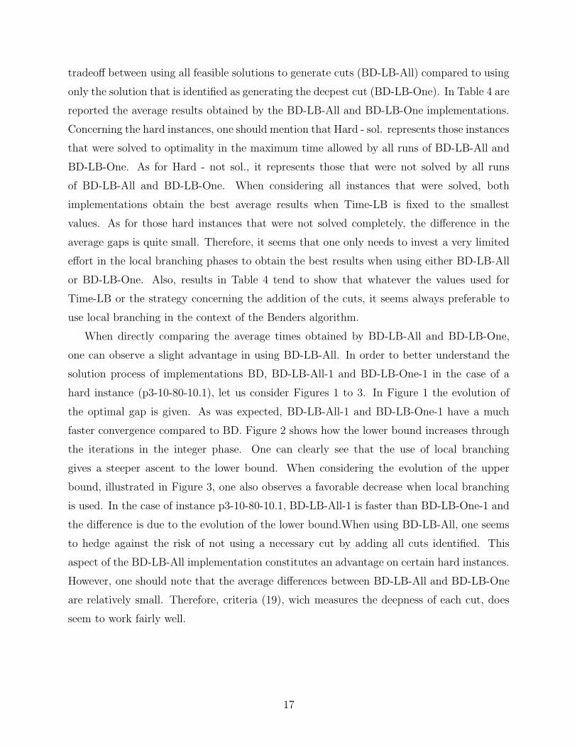
When directly comparing the average times obtained by BD-LB-All and BD-LB-One,

one can observe a slight advantage in using BD-LB-All. In order to better understand the

solution process of implementations BD, BD-LB-All-1 and BD-LB-One-1 in the case of a

hard instance (p3-10-80-10.1), let us consider Figures 1 to 3. In Figure 1 the evolution of

the optimal gap is given. As was expected, BD-LB-All-1 and BD-LB-One-1 have a much

faster convergence compared to BD. Figure 2 shows how the lower bound increases through

the iterations in the integer phase. One can clearly see that the use of local branching

gives a steeper ascent to the lower bound. When considering the evolution of the upper

bound, illustrated in Figure 3, one also observes a favorable decrease when local branching

is used. In the case of instance p3-10-80-10.1, BD-LB-All-1 is faster than BD-LB-One-1 and

the difference is due to the evolution of the lower bound.When using BD-LB-All, one seems

to hedge against the risk of not using a necessary cut by adding all cuts identified. This

aspect of the BD-LB-All implementation constitutes an advantage on certain hard instances.

However, one should note that the average differences between BD-LB-All and BD-LB-One

are relatively small. Therefore, criteria (19), wich measures the deepness of each cut, does

seem to work fairly well.

17

Instances BD BD-LB-All-2p1-10-50-10.1 24.8 17.9p1-10-50-10.2 85.94 40.03p1-10-50-15.1 3417.31 467.7p1-10-50-15.2 1706.55 344.98p2-10-50-10.1 6321.1 1008.84p2-10-50-10.2 70.66 36.67p2-10-50-15.1 927.44 127.64p2-10-50-15.2 19.58 6.45p3-10-50-10.1 13.34 53.92p3-10-50-10.2 5.01 20.72p3-10-50-15.1 73.51 21.74p3-10-50-15.2 57.91 35.88p4-10-50-10.1 480.94 16.84p4-10-50-10.2 1249.43 19.1p4-10-50-15.1 > 10000, 11.11% > 10000, 3.56%p4-10-50-15.2 1455.82 332.21p5-10-50-10.1 8.05 10.17p5-10-50-10.2 12.94 54.64p5-10-50-15.1 60.76 5.48p5-10-50-15.2 25.75 5.6p1-10-60-10.1 106.84 103.82p1-10-60-10.2 96.33 158.02p1-10-60-15.1 20.94 8.35p1-10-60-15.2 3321.01 450.14p2-10-60-10.1 6095.9 1002.86p2-10-60-10.2 659.71 50.51p2-10-60-15.1 > 10000, 10.10 % 9548.79p2-10-60-15.2 407.48 118.94p3-10-60-10.1 > 10000, 9.14 % 1239.2p3-10-60-10.2 1.9 1.3p3-10-60-15.1 > 10000, 7.94 % > 10000, 4.92%p3-10-60-15.2 2974.62 966.4p4-10-60-10.1 40.09 151.25p4-10-60-10.2 1.28 1.24p4-10-60-15.1 > 10000, 9.83 % > 10000, 2.33%p4-10-60-15.2 > 10000, 3.74% > 10000, 1.88%p5-10-60-10.1 104.29 5.25p5-10-60-10.2 4.55 6.77p5-10-60-15.1 > 10000, 1.20% 2473.26p5-10-60-15.2 233.49 3.82

Table 1: BD vs. BD-LB-All-2

18

Instances BD BD-LB-All-2p1-10-70-10.1 > 10000, 12.70% 7187.6p1-10-70-10.2 > 10000, 8.80% 6560.24p1-10-70-15.1 13.83 40.61p1-10-70-15.2 5281.74 424.94p2-10-70-10.1 1773.31 404.77p2-10-70-10.2 3.16 1.41p2-10-70-15.1 > 10000, 23.40% > 10000, 8.15%p2-10-70-15.2 > 10000, 1.57% 1051.98p3-10-70-10.1 1080.95 316.23p3-10-70-10.2 1167.13 338.17p3-10-70-15.1 > 10000, 11.37% > 10000, 4.83%p3-10-70-15.2 > 10000, 18.13% > 10000, 13.64%p4-10-70-10.1 1126.25 192.65p4-10-70-10.2 310.38 171.33p4-10-70-15.1 2453.59 1017.95p4-10-70-15.2 165.55 114.5p5-10-70-10.1 31.26 18.03p5-10-70-10.2 5.67 2.34p5-10-70-15.1 > 10000, 6.19% > 10000, 5.44%p5-10-70-15.2 1187.8 685.88p1-10-80-10.1 502.08 39.77p1-10-80-10.2 160.04 343.57p1-10-80-15.1 > 10000, 11.39% > 10000, 8.92%p1-10-80-15.2 > 10000, 7.20% > 10000, 2.55%p2-10-80-10.1 > 10000, 2.80% 2089.08p2-10-80-10.2 635.03 605.22p2-10-80-15.1 > 10000, 22.41% > 10000, 17.37%p2-10-80-15.2 3725.01 798.71p3-10-80-10.1 > 10000, 1.19% 6520.39p3-10-80-10.2 358.41 547.62p3-10-80-15.1 > 10000, 5.70% > 10000, 3.3%p3-10-80-15.2 > 10000, 1.006% 2350.7p4-10-80-10.1 2773.39 329.15p4-10-80-10.2 3479.37 2368.79p4-10-80-15.1 > 10000, 18.21% > 10000, 8.28%p4-10-80-15.2 > 10000, 3.39% > 10000, 2.10%p5-10-80-10.1 > 10000, 5.47% 7011.97p5-10-80-10.2 > 10000, 4.52% > 10000, 1.37%p5-10-80-15.1 > 10000, 6.09% > 10000, 2.65%p5-10-80-15.2 6811.16 1770.05

Table 2: BD vs. BD-LB-All-2

19

BD BD-LB-All-2Measures easy moderate hard easy moderate hard

Ave. 163.68 sec. 3021.13 sec. 10.66% 84.21 sec. 696.82 sec. 5.71%Var. 53071.32 3565790.57 42.56 20166.66 332003.6 20.73S.D. 230.37 sec. 1888.33 sec. 6.52% 142.01 sec. 576.2 sec. 4.55%Fea. 21.54 82.53 - 8.66 32.26 -Opt. 65.91 272.47 - 37.14 131.53 -

Nb. It. 102.03 356 - 19.69 78.47 -

Table 3: BD vs. BD-LB-All-2

BD-LB-All BD-LB-OneInstances 1 2 3 1 2 3

Easy (sec.) 51.11 84.21 142.65 54.31 79.48 168.25Moderate (sec.) 643.36 696.82 1162.75 691.11 831.96 1304.1Hard - sol. (sec.) 2788.45 3662.1 4784.63 3011.77 3139.48 3822.59

Hard - not sol. (%) 6.61 6.2 6.64 6.27 6.83 6.68

Table 4: BD-LB-All vs. BD-LB-One

BD BD-LB-One-1 BD-LB-All-1Instances Time (sec.) Gap Time (sec.) Gap Time (sec.) Gap

p20-70-10.1 > 30, 000 12.37% > 30, 000 8.23% > 30, 000 11.22%p20-70-10.2 1411.71 < 1% 685.20 < 1% 364.60 < 1%p20-70-15.1 > 30, 000 6.97% 25177.90 < 1% 19844.35 < 1%p20-70-15.2 > 30, 000 7.31% > 30, 000 3.20% > 30, 000 2.43%

Table 5: 2nd Phase Tests

20

0

0.05

0.1

0.15

0.2

0.25

0.3

0.35

0 2000 4000 6000 8000 10000 12000

Eps

ilon

valu

e

Time (sec.)

BDBD-LB-All

BD-LB-One

Figure 1: Time vs. Gap for p3-10-80-10.1

In order to validate the observations made so far, a second set of tests was obtained on

instances based on larger networks (Table 5). For this second set of tests, the maximum time

allowed was increased to 30,000 seconds. Also, since the previous tests seemed to demonstrate

that, when using local branching in the Benders algorithm, one usually obtained the best

results when Time-LB was fixed to the smallest values, Time-LB was set to 2.5 seconds for

all runs in Table 5.

These new results confirm previous observations. Once again, the use of local branching

gives an added advantage when compared to BD. On these new instances, BD-LB-All also

seems to be better compared to BD-LB-One. In the case of p20-70-10.2, BD-LB-All is about

2 times faster than BD-LB-One. As for p20-70-15.1, BD-LB-All obtains a relative reduction

in solution time of 21.18% when compared to BD-LB-One.

5 Conclusion

This paper proposes a novel way to accelerate the Benders decomposition algorithm by using

local branching. By doing a local branching search after each master problem solved in the

integer phase of the Benders algorithm, one can explore the neighborhood of the solution

obtained for the master problem, which may or may not be feasible, in order to find different

feasible solutions. By doing so, one can obtain better upper bounds at each iteration and

since each different feasible solution can be used to generate an optimality cut, one can also

21

41500

42000

42500

43000

43500

44000

44500

45000

45500

46000

46500

0 100 200 300 400 500 600 700

Low

er b

ound

Int. iterations

BDBD-LB-All

BD-LB-One

Figure 2: Int. iterations vs. Lower bound for p3-10-80-10.1

simultaneously obtain better lower bounds. Furthermore, the subproblems that are found to

be infeasible during the local branching phases can be used as a way to complement or replace

the feasibility cuts added during the solution process. Therefore, all information obtained

through the local branching strategy can be used in the context of Benders decomposition.

Finally, since local branching only requires the use of a solver, if one can apply the

Benders algorithm to the problem at hand then the same Benders algorithm can be used as

this optimizer. This makes the use of local branching possible for all 0-1 integer problems

that can be solved by Benders decomposition. Numerical tests in this paper have shown

how local branching can greatly improve the performance of the standard Benders algorithm

in the case of an integer linear problem (the MCFND problem). Recently, applications of

Benders decomposition have focussed on non-linear or non-convex optimization problems.

Clearly one interesting avenue of research would therefore be to verify that the acceleration

technique proposed here remains as efficient in those settings.

References

Benders, J.F. 1962. Partitioning procedures for solving mixed-variables programming prob-

lems. Numerische Mathematik 4 238–252.

Codato, G., M. Fischetti. 2004. Combinatorial benders cuts for mixed-integer linear pro-

22

46000

48000

50000

52000

54000

56000

58000

60000

62000

64000

0 100 200 300 400 500 600 700

Upp

er b

ound

Int. iterations

BDBD-LB-All

BD_LB-One

Figure 3: Int. iterations vs. Upper bound for p3-10-80-10.1

gramming. D. Bienstock, G. Nemhauser, eds., Integer Programming and Combinatorial

Optimization. Lectures Notes in Computer Science: Springer-Verlag, 178–195.

Costa, A.M. 2005. A survey on benders decomposition applied to fixed-charge network design

problems. Computers and operations research 32 1429–1450.

Cote, G., M.A. Laughton. 1984. Large-scale mixed integer programming: Benders-type

heuristics. European Journal of Operational Research 16 327–333.

Crainic, T.G., A. Frangioni, B. Gendron. 2002. Bundle-based relaxation methods for mul-

ticommodity capacitated fixed charge network design problems. Discrete Applied Mathe-

matics 112 73–99.

Fischetti, M., A. Lodi. 2003. Local branching. Mathematical Programming 98 23–47.

Geoffrion, A.M. 1970a. Elements of large-scale mathematical programming part 1: Concepts.

Management Science 11 652–675.

Geoffrion, A.M. 1970b. Elements of large-scale mathematical programming part 2: Synthesis

of algorithms and bibliography. Management Science 11 676–691.

Holmberg, K. 1990. On the convergence of cross decomposition. Mathematical Programming

47 269–296.

23

Holmberg, K. 1994. On using approximations of the benders master problem. European

Journal of Operational Research 77 111–125.

Hooker, J.N. 2000. Logic-Based Methods for Optimization: Combining Optimization and

Constraint Satisfaction. John Wiley and Sons.

Magnanti, T.L., R.T. Wong. 1981. Accelerating benders decomposition algorithmic enhance-

ment and model selection criteria. Operations Research 29 464–484.

McDaniel, D., M. Devine. 1977. A modified benders’partitioning algorithm for mixed integer

programming. Management Science 24 312–319.

Roy, T.J. Van. 1983. Cross decomposition for mixed integer programming. Mathematical

Programming 25 46–63.

24