Decomposition Algorithm 02 - Iran University of Science...

In the name of GodIn the name of God

Part 4. Decomposition Algorithms

4.2. Benders’ Decomposition

Algorithm

Decomposition Algorithms

Algorithm

Spring 2010Instructor: Dr. Masoud Yaghini

Benders Decomposition Algorithm



� The Dantzig-Wolfe decomposition procedure is

equivalent for linear programming problems to two

other well known partitioning / decomposition /

relaxation techniques:

– Benders decomposition / partitioning method

– Lagrangian relaxation method


– Lagrangian relaxation method


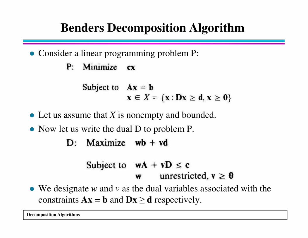
� Consider a linear programming problem P:

� Let us assume that X is nonempty and bounded.


� Let us assume that X is nonempty and bounded.

� Now let us write the dual D to problem P.

� We designate w and v as the dual variables associated with the

constraints Ax = b and Dx ≥ d respectively.


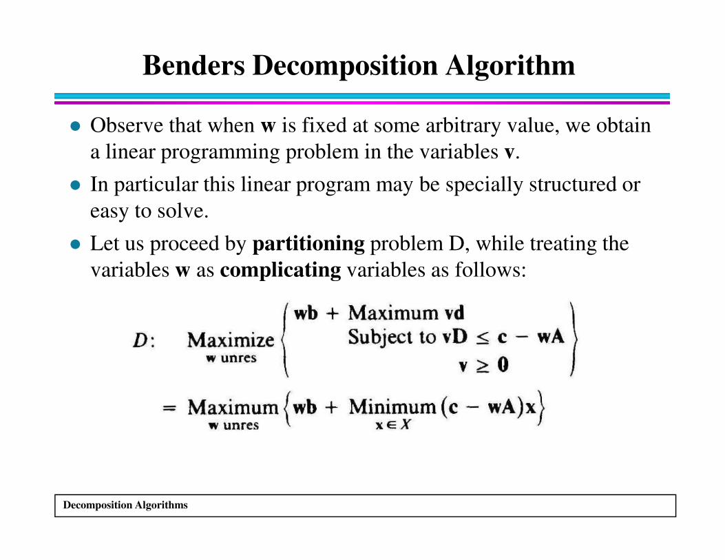
� Observe that when w is fixed at some arbitrary value, we obtain

a linear programming problem in the variables v.

� In particular this linear program may be specially structured or

easy to solve.

� Let us proceed by partitioning problem D, while treating the

variables w as complicating variables as follows:


variables w as complicating variables as follows:


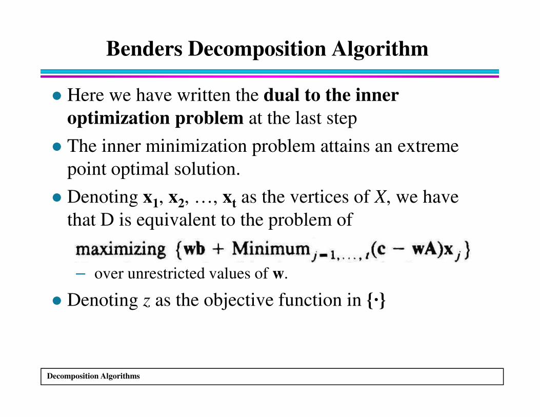
� Here we have written the dual to the inner

optimization problem at the last step

� The inner minimization problem attains an extreme

point optimal solution.

� Denoting x1, x2, …, xt as the vertices of X, we have

that D is equivalent to the problem of


1 2 t

that D is equivalent to the problem of

– over unrestricted values of w.

� Denoting z as the objective function in {·}


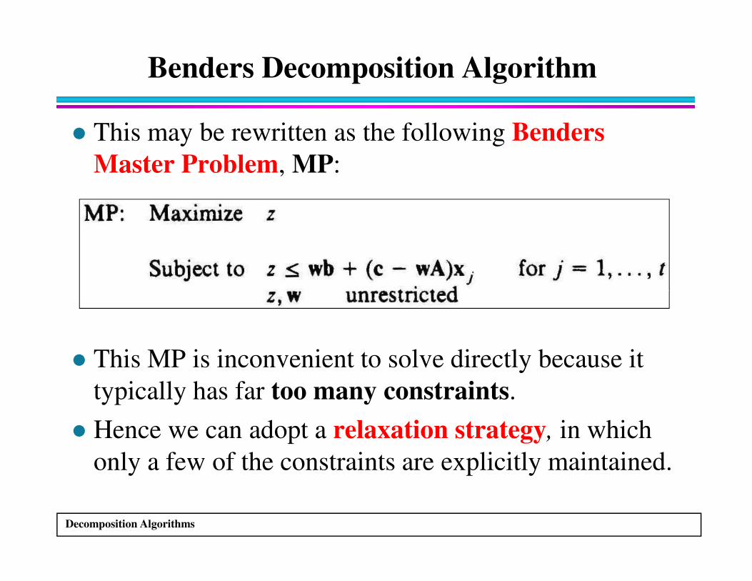
� This may be rewritten as the following Benders

Master Problem, MP:


� This MP is inconvenient to solve directly because it

typically has far too many constraints.

� Hence we can adopt a relaxation strategy, in which

only a few of the constraints are explicitly maintained.


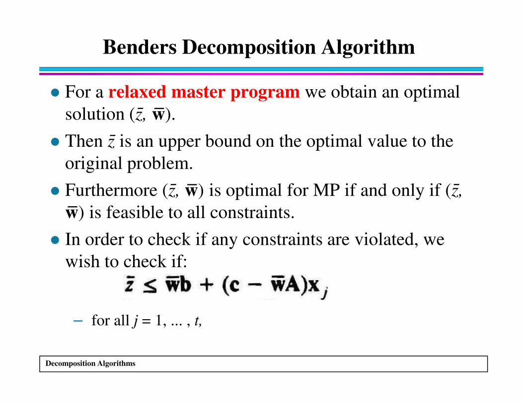
� For a relaxed master program we obtain an optimal

solution (z̄, w̅).

� Then z̄ is an upper bound on the optimal value to the

original problem.

� Furthermore (z̄, w̅) is optimal for MP if and only if (z̄,

w̅) is feasible to all constraints.


w̅

w̅) is feasible to all constraints.

� In order to check if any constraints are violated, we

wish to check if:

– for all j = 1, ... , t,


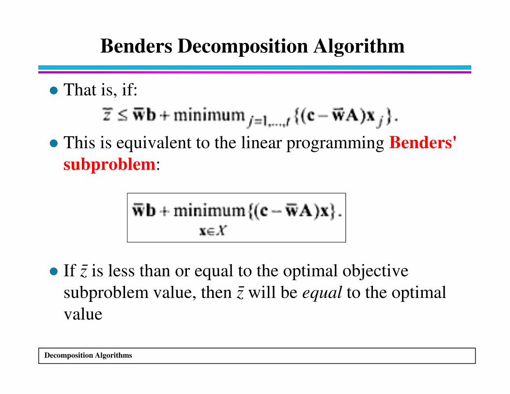
� That is, if:

� This is equivalent to the linear programming Benders'

subproblem:


� If z̄ is less than or equal to the optimal objective

subproblem value, then z̄ will be equal to the optimal

value


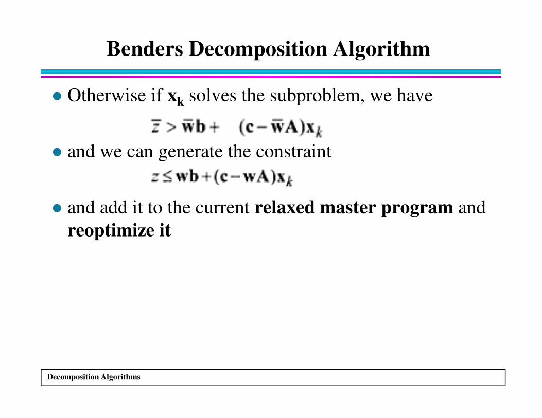
� Otherwise if xk solves the subproblem, we have

� and we can generate the constraint

� and add it to the current relaxed master program and


� and add it to the current relaxed master program and

reoptimize it


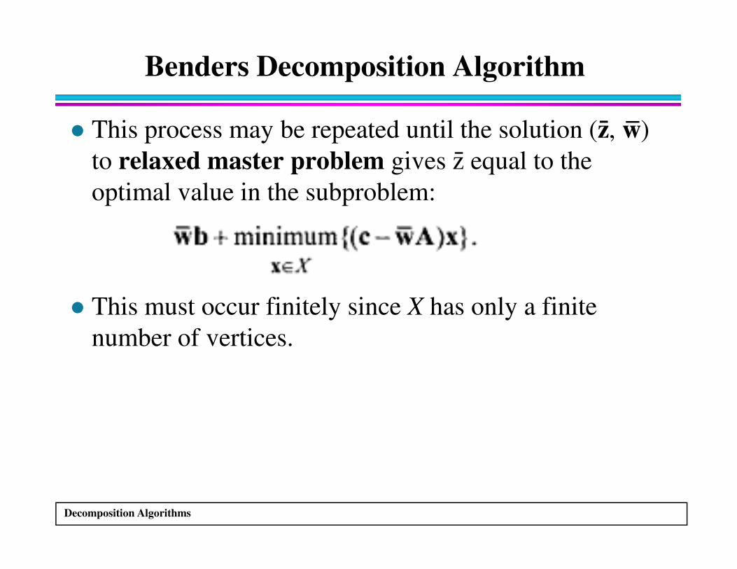
� This process may be repeated until the solution (z̄, w̅)

to relaxed master problem gives z̄ equal to the

optimal value in the subproblem:


� This must occur finitely since X has only a finite

number of vertices.


� Note that the Benders subproblem is also the

subproblem solved by the Dantzig-Wolfe

decomposition method

� And the Benders master program is simply the dual

to the Dantzig-Wolfe master problem with

constraints.


constraints.

� Here the nonnegative dual multipliers associated with

the constraints are λj, j = 1, 2, …., t , these variabls

sum to unity by virtue of the column of the variables


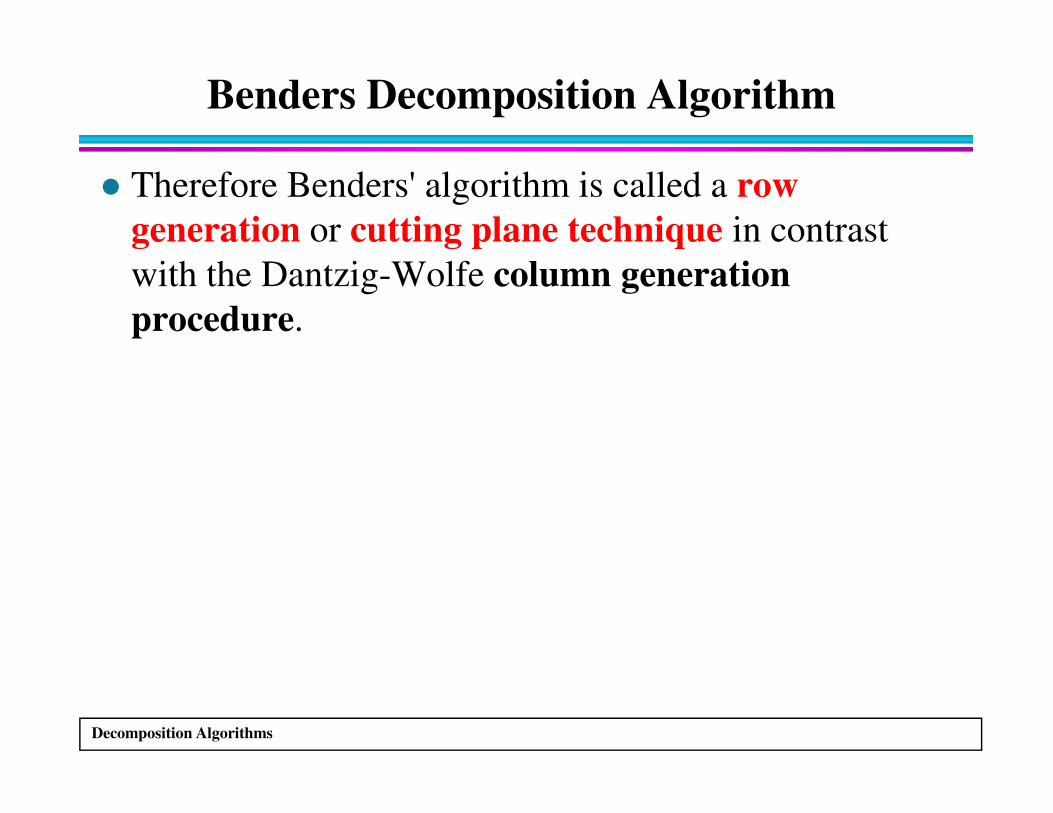
� Therefore Benders' algorithm is called a row

generation or cutting plane technique in contrast

with the Dantzig-Wolfe column generation

procedure.


Lagrangian Relaxation Algorithm

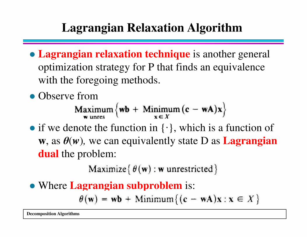
� Lagrangian relaxation technique is another general

optimization strategy for P that finds an equivalence

with the foregoing methods.

� Observe from


� if we denote the function in {·}, which is a function of

w, as θ(w), we can equivalently state D as Lagrangian

dual the problem:

� Where Lagrangian subproblem is:

Numeric Example


Numeric Example

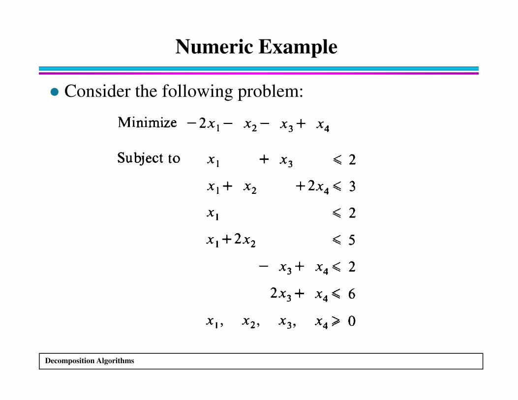
� Consider the following problem:


Numeric Example

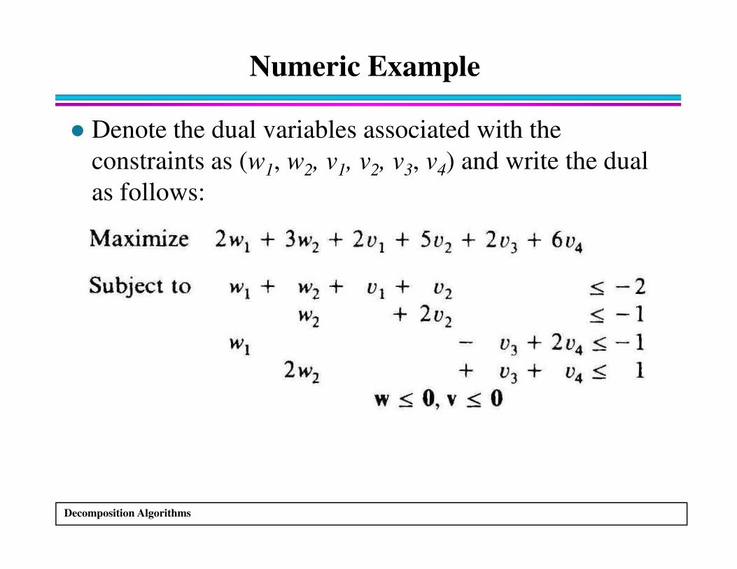
� Denote the dual variables associated with the

constraints as (w1, w2, v1, v2, v3, v4) and write the dual

as follows:


Numeric Example

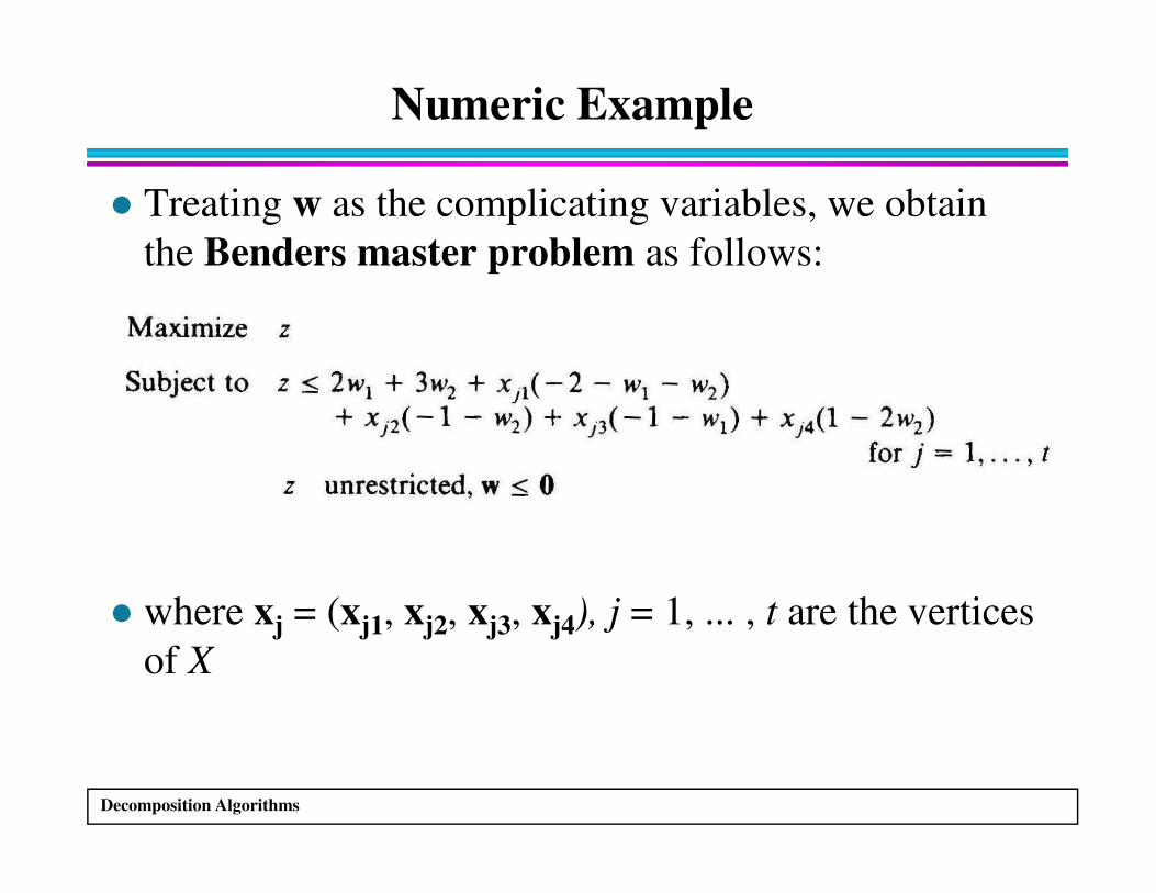
� Treating w as the complicating variables, we obtain

the Benders master problem as follows:


� where xj = (xj1, xj2, xj3, xj4), j = 1, ... , t are the vertices

of X

Numeric Example

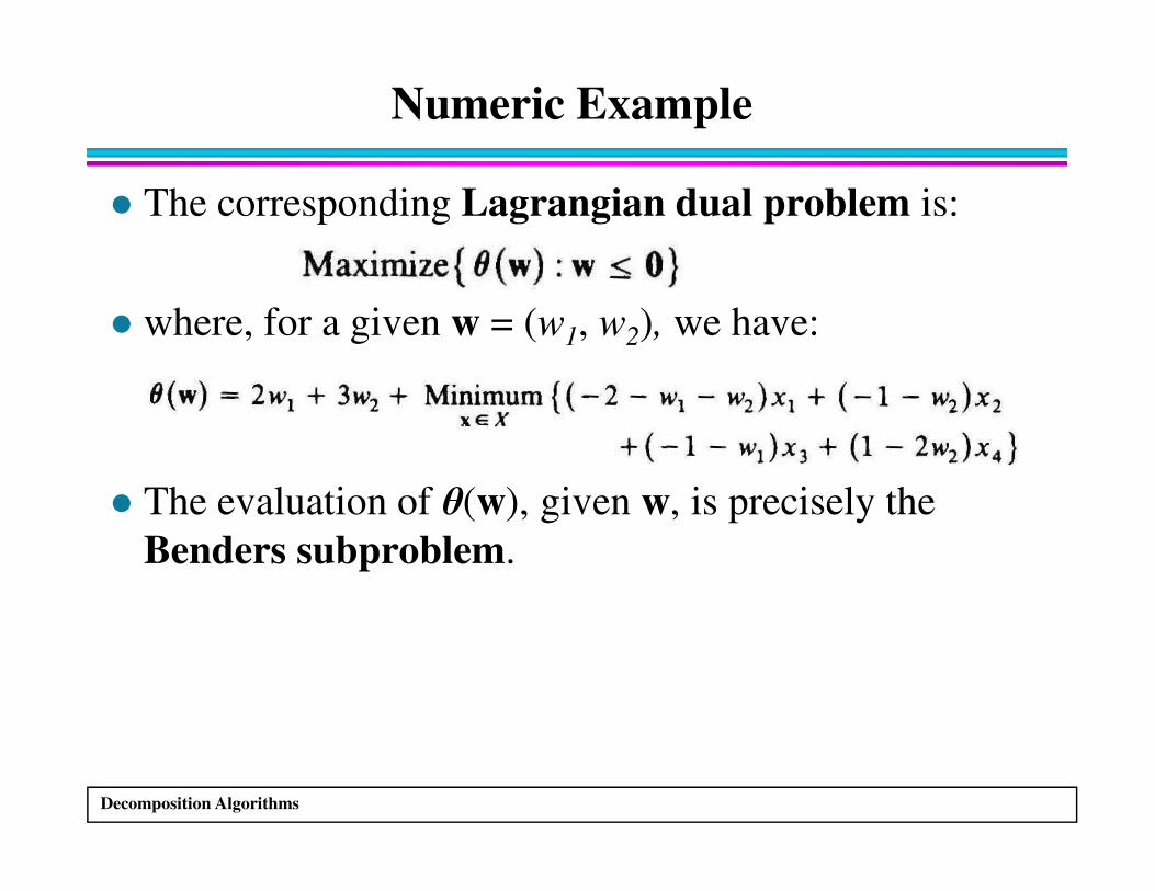
� The corresponding Lagrangian dual problem is:

� where, for a given w = (w1, w2), we have:


� The evaluation of θ(w), given w, is precisely the

Benders subproblem.

Numeric Example

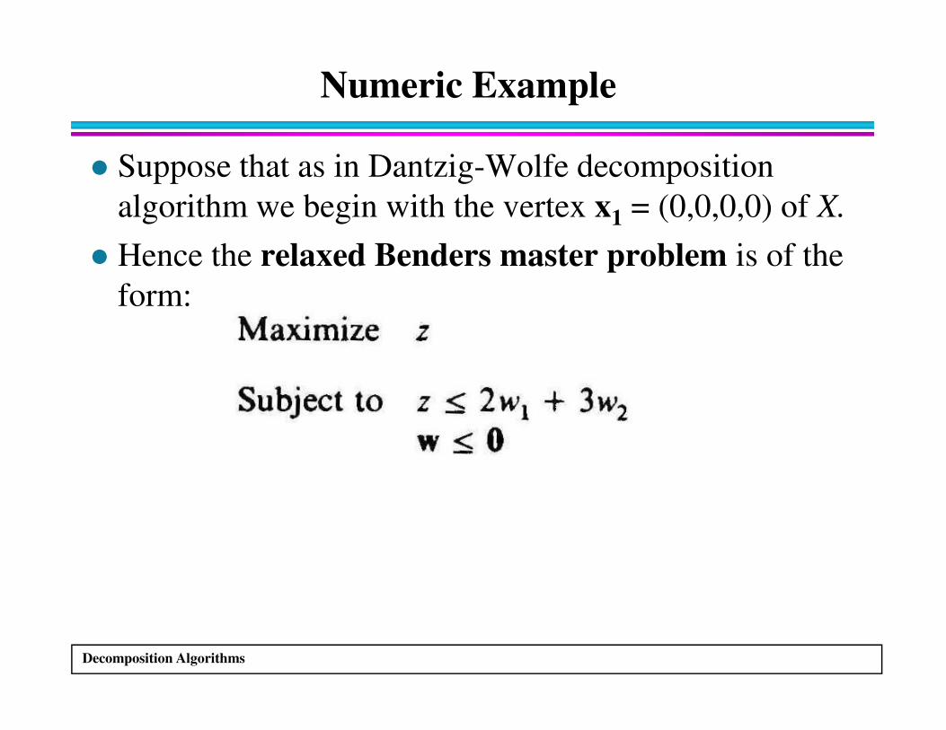
� Suppose that as in Dantzig-Wolfe decomposition

algorithm we begin with the vertex x1 = (0,0,0,0) of X.

� Hence the relaxed Benders master problem is of the

form:


Numeric Example

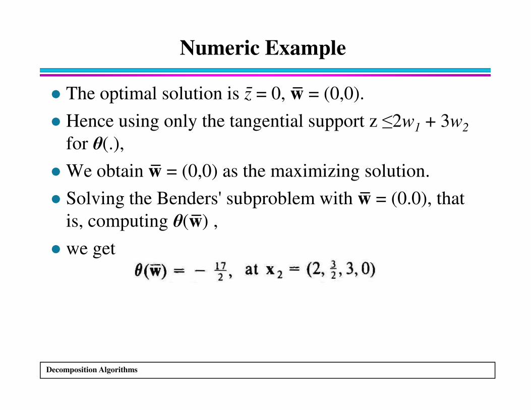
� The optimal solution is z̄ = 0, w̅ = (0,0).

� Hence using only the tangential support z ≤2w1 + 3w2

for θ(.),

� We obtain w̅ = (0,0) as the maximizing solution.

� Solving the Benders' subproblem with w̅ = (0.0), that


� Solving the Benders' subproblem with w̅ = (0.0), that

is, computing θ(w̅) ,

� we get

Numeric Example

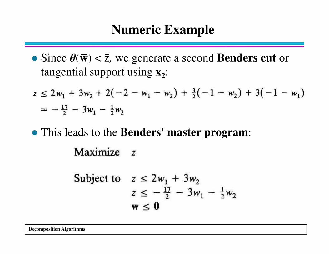
� Since θ(w̅) < z̄, we generate a second Benders cut or

tangential support using x2:

This leads to the Benders' master program:


� This leads to the Benders' master program:

Numeric Example

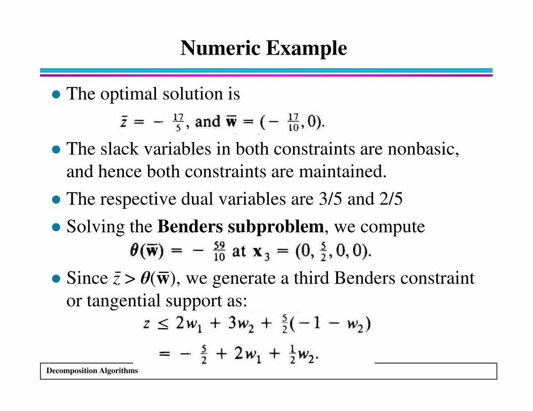
� The optimal solution is

� The slack variables in both constraints are nonbasic,

and hence both constraints are maintained.

� The respective dual variables are 3/5 and 2/5


� The respective dual variables are 3/5 and 2/5

� Solving the Benders subproblem, we compute

� Since z̄ > θ(w̅), we generate a third Benders constraint

or tangential support as:

Numeric Example

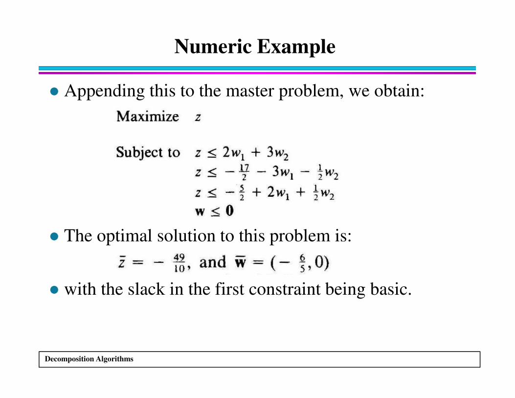
� Appending this to the master problem, we obtain:


� The optimal solution to this problem is:

� with the slack in the first constraint being basic.

Numeric Example

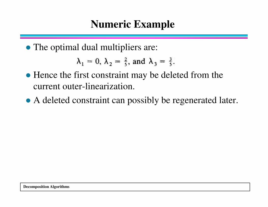
� The optimal dual multipliers are:

� Hence the first constraint may be deleted from the

current outer-linearization.

� A deleted constraint can possibly be regenerated later.


� A deleted constraint can possibly be regenerated later.

References


References

� M.S. Bazaraa, J.J. Jarvis, H.D. Sherali, Linear

Programming and Network Flows, Wiley, 1990.

(Chapter 7)


The End


Date post:	25-Jun-2018
Category:	Documents
Upload:	vuongnga
View:	236 times
Download:	0 times

Decomposition Algorithm 02 - Iran University of Science...

Documents