Acceleration and Deceleration Detection and Baseline...

Acceleration and Deceleration Detection and Baseline Estimation Master of Science Thesis in the Master Degree Programme Biomedical Engineering

SUSANNE ANDERSSON Department of Signals and Systems Division of Biomedical Engineering CHALMERS UNIVERSITY OF TECHNOLOGY Göteborg, Sweden, 2011 Report No. EX037/2011

REPORT NO. EX037/2011

Acceleration and Deceleration Detection and Baseline Estimation

Master’s Thesis in the Master’s programme Biomedical Engineering

SUSANNE ANDERSSON

Department of Signals and Systems Division of Biomedical Engineering

CHALMERS UNIVERSITY OF TECHNOLOGY Göteborg, Sweden 2011

Acceleration and Deceleration Detection and Baseline Estimation Master’s Thesis in the Master’s programme Biomedical Engineering SUSANNE ANDERSSON © SUSANNE ANDERSSON, 2011

Report No. EX037/2011 Department of Signals and Systems Division of Biomedical Engineering Chalmers University of Technology SE-412 96 Göteborg Sweden Telephone: + 46 (0)31-772 1000 Cover: Registration of fetal heart rate and uterine contractions (Neoventa Medical AB 2008). Department of Signals and Systems Göteborg, Sweden, 2011

Acceleration and Deceleration Detection and Baseline Estimation Master’s Thesis in the Master’s programme Biomedical Engineering SUSANNE ANDERSSON Department of Signals and Systems Division of Biomedical Engineering Chalmers University of Technology

ABSTRACT CTG monitoring of the fetal heart rate and uterine contractions during pregnancy and delivery provide information on the physiological condition of the fetus needed to identify hypoxia. Interpretation, however, requires experience and important patterns might be missed or misinterpreted due to stress, exhaustion or distraction. Interpretation has also been reported subjective with poor reproducibility. Computerized analysis of the fetal heart rate could help overcome these issues and provide fully reproducible analysis.

The aim of this thesis is to evaluate algorithms for automated detection of fetal heart rate accelerations and decelerations and estimating the basal heart rate, for fetal monitoring during labor.

Algorithms have been developed and the performance has been compared to the opinions of clinical experts and to other competing algorithms.

Disagreement between clinical experts is considerably high for both acceleration and deceleration detection, but the observers are fairly consistent in estimating the basal heart rate.

The developed algorithms all perform better than the competing algorithms and the performance is within or close to the uncertainty between the clinical experts.

Key words: CTG, fetal monitoring, automated analysis, baseline, basal heart rate,

accelerations, decelerations, inter-observer variability, intra-observer variability

Preface This thesis is the result from a master’s thesis project carried out at Neoventa Medical in Mölndal, Sweden, from January 2011 to June 2011, for a degree in the master’s programme Biomedical Engineering at Chalmers Technical University, Göteborg, Sweden.

Supervisor at Neoventa Medical was PhD Nils Löfgren, who provided guidance and valuable input throughout the project. Examiner, at the department of Signals and Systems at Chalmers Technical University, was Senior Lecturer Ants Silberberg.

A prerequisite for the existence of this thesis was the contributions from midwifes Annika Mårtendal and Ulla-Stina Wilson, both employed by Neoventa Medical. They invested time and effort in helping me with CTG assessments, for which I am grateful.

Göteborg June 2011 Susanne Andersson

List of terms

Antepartum Time before labor

Bradycardia Basal heart rate below 110 bpm

Electrocardiogram, ECG Recording of the electrical activity of the heart

Hypoxia Inadequate supply of oxygen

Inter-observer agreement Measure of agreement when different individuals perform the same task

Intra-observer agreement Measure of agreement when the same task is performed at different occasions by the same individual

Intrapartum Time during labor

Pathological Condition relating to disease

Tachycardia Basal heart rate above 160 bpm

Table of Contents 1. Introduction ...................................................................................................................1

1.1 Aim and objectives ...................................................................................................2

1.2 Delimitations ............................................................................................................2

2. Methods .........................................................................................................................4

2.1 Preprocessing ...........................................................................................................5

2.2 Running baseline estimation .....................................................................................8

2.2.1 Algorithm by Dawes et al. .................................................................................8

2.2.2 Modification of the algorithm by Dawes et al. ...................................................9

2.2.3 Algorithm 1 .......................................................................................................9

2.2.4 Algorithm 2 ..................................................................................................... 14

2.3 Acceleration detection ............................................................................................ 16

2.4 Deceleration detection ............................................................................................ 16

2.5 Basal heart rate ....................................................................................................... 16

2.5.1 Algorithms by Dawes et al. and Ayres-de-Campos et al. .................................. 17

2.5.2 Algorithm A .................................................................................................... 17

2.5.3 Algorithm B .................................................................................................... 18

2.5.4 Undefined by expert observer .......................................................................... 19

3. Results .......................................................................................................................... 20

3.1 Acceleration detection ............................................................................................ 20

3.1.1 Observer uncertainty ....................................................................................... 20

3.1.2 Testing ............................................................................................................ 20

3.1.3 Validation ....................................................................................................... 22

3.2 Deceleration detection ............................................................................................ 23


3.2.2 Testing ............................................................................................................ 23

3.2.3 Validation ....................................................................................................... 25

3.3 Basal heart rate ....................................................................................................... 26


3.3.2 Testing ............................................................................................................ 26

3.3.3 Validation ....................................................................................................... 27

4. Discussion .................................................................................................................... 28

4.1 Acceleration and deceleration detection .................................................................. 29

4.1.1 Alternative methods ........................................................................................ 30

4.1.2 Impact of observer uncertainty ........................................................................ 31

4.2 Basal heart rate ....................................................................................................... 32

4.3 Gathering of expert observer opinions .................................................................... 36

4.4 Clinical impact of the results .................................................................................. 37

5. Conclusions .................................................................................................................. 38

6. References .................................................................................................................... 39

Appendix A – Algorithm 1 with acceleration detection

Appendix B – Algorithm 1 with deceleration detection

Appendix C – Algorithm 2 with acceleration detection

Appendix D – Algorithm 2 with deceleration detection

Appendix E – Algorithm A and algorithm B

Appendix F – Basal heart rate estimation by SisPorto

1

1. Introduction Cardiotocography (CTG) refers to monitoring the fetal heart rate and the uterine contractions during late pregnancy and delivery (Neoventa Medical AB, 2008). Interpretation of the fetal heart rate levels, changes and correlation to the uterine contractions will provide the experienced clinician with the information on the physiological condition of the fetus needed to identify hypoxia and take actions before permanent brain damage or death occurs (Ingemarsson 2006).

Correct interpretation requires experience and important patterns in the trace might be missed or misinterpreted due to stress, exhaustion or distraction. Interpretation of the fetal heart rate trace has also been reported subjective with poor reproducibility (Beaulieu 1982, Bernardes 1997, Ayres-de-Campos 1999, Devane 2005, Chauhan 2008, Westerhuis 2009).

The indistinctness of how to assess the fetal heart rate trace led the National Institute of Child Health and Human Development to define guidelines for the interpretation (Macones 2008). Parameters essential for this thesis are fetal heart rate baseline, accelerations and decelerations. Baseline, expressed in beats per minute (bpm), is defined as the approximate mean fetal heart rate during at least ten minutes of stable segments, excluding accelerations and decelerations. Acceleration is defined as an increase in heart rate from the baseline, lasting for at least 15 seconds, with a peak of at least 15 bpm above the baseline. Equivalently, a deceleration is defined as a decrease in heart rate from the baseline for at least 15 seconds, during which at least one sample is 15 bpm below baseline. See figure 1.

Figure 1. Fetal heart rate trace containing one acceleration and one deceleration.

STAN S31, manufactured by Neoventa Medical, is a system for intrapartum fetal monitoring combining the traditional CTG with ST-analysis of the fetal electrocardiogram (ECG). The apparatus generates alarms at hypoxia related abnormalities in the ST segment of the ECG pattern, corresponding to the heart muscles adjusting to lack of oxygen.

STAN S31 measures the heart rate using ultrasound transducers before the membranes are ruptured, and then using an electrode on the fetal scalp. The ECG is obtained from the scalp

2

electrode using a reference on the mother’s thigh. Automated estimation of the baseline or detection of accelerations and decelerations is not available in STAN S31 today. It would however be a valuable complement to the ST analysis since ST changes should always be assessed in relation to the CTG. Automated heart rate analysis would assist the staff in interpreting the trace in stressful situations.

The Dawes/Redman criteria (Dawes 1982) are a set of algorithms developed for antepartum CTG analysis, aiming to help predict fetal outcome. The trace is assessed as normal or pathological based on these criteria. It is widely clinically implemented and there has been a demand for implementation of these criteria or similar analysis in STAN. SisPorto (Ayres-de-Campos 2000) is another system for automated fetal heart rate analysis, antepartum and intrapartum, also clinically implemented. For this thesis, its estimation of basal heart rate has been of specific interest.

1.1 Aim and objectives The aim of this thesis is to evaluate the possibility of implementing algorithms for automated detection of accelerations and decelerations, and estimating the basal heart rate, into a system for fetal monitoring during labor. These algorithms should perform within the uncertainty between clinical experts, or with higher accuracy.

The objectives are to:

§ gather expert opinions on cardiotocographic events to be used as reference data § evaluate inter-observer agreement between clinical experts for uncertainty of the

reference data § develop algorithms for automated detection of accelerations and decelerations and

estimation of basal heart rate, for heart rate signals obtained from either ultrasound or fetal scalp electrode

§ compare the performance of these with competing algorithms in clinical use

The Dawes/Redman criteria utilize, among others, the parameters of interest for this thesis: estimated basal heart rate, accelerations and decelerations. Hence, performance of the algorithms is compared to that of those described by Dawes et al. For basal heart rate estimation, the algorithm described by Ayres-de-Campos et al. is also implemented and tested.

1.2 Delimitations Since the purpose of this thesis is only to detect the patterns from a given heart rate signal, no profound research have been carried out regarding the actual physiological background of basal heart rate or accelerations and decelerations occurring.

Numerous algorithms for automated cardiotocographic analysis have been proposed over the years (Dawes 1982, Skinner 1999, Ayres-de-Campos 2000, Taylor 2000, Jimenez 2002, Warrick 2005), and all could not possibly be evaluated. Discussion with employees at Neoventa Medical familiar with the subject led to limitation to only the competing algorithms of highest interest for the company.

3

Clinical evaluation of the cardiotocograms is time consuming. For the scope of this thesis, involving two clinical experts for evaluation of the registrations was considered the realistic alternative. For the same reason the amount of registrations observed had to be limited accordingly.

4

2. Methods Algorithms for baseline estimation, as well as acceleration and deceleration detection, have been implemented both by recreating previously published work, and by developing improved algorithms. All algorithms were implemented and evaluated using Matlab. The algorithms described by Dawes et al. have been implemented reusing Matlab code from a previous work (Lätt Nyboe 2011). The algorithms have proven to imitate the original Dawes/Redman algorithms well.

Evaluation of the algorithm performance requires estimates of which outcomes that are valid and which are not. Because of the interdependence of the baseline definition and the acceleration and deceleration definitions there is no absolute standard for this verification. It is subjective, and which cardiotocographic events are present have to be determined based on opinions of experienced clinicians. Two midwifes assisted in interpreting fetal heart rate traces. The traces were randomly selected intrapartum recordings with duration between 16 minutes to ten hours and 18 minutes. Observer 1, Annika Mårtendal interpreted all of the traces and acted as gold standard when testing and verifying the validity of the algorithm outcomes. Hence, the algorithms have been built to match the opinions of this observer. Observer 2, Ulla-Stina Wilson, independently interpreted only the traces that would later be used during validation, aiming to provide the possible uncertainty between the two experts. The performance by any algorithm against the opinions of observer 1 cannot be required more accurate than the performance by observer 2 against the opinions of observer 1.

The number of traces for which observer 1 and observer 2 marked the occurrences of accelerations and decelerations, as well as estimating the basal heart rates, is seen in figure 2.

Figure 2. Number of CTG traces evaluated by observer 1 and observer 2.

Acceleration detection50 traces

Test

40 traces

Observer 1

Validation

10 traces

Observer 1 Observer 2

Deceleration detection31 traces

Test

21 traces

Observer 1

Validation

10 traces


Basal heart rate estimation100 traces

Test

50 traces

Observer 1

Validation

50 traces


5

The performance of the algorithms for acceleration detection and deceleration detection were tested against the opinions of observer 1. For this evaluation, the statistical measures sensitivity and positive predictive value were used. These are, in the case of acceleration detection defined as

sensitivity = numberoftruedetectedaccelerations

numberofactualaccelerations

positivepredictivevalue = numberoftruedetectedaccelerations

totalnumberofdetections

The sensitivity and positive predictive value are analogously defined also for evaluation of the deceleration detection performance.

Testing of the algorithms was performed repeatedly. One or two parameters were varied with the purpose of finding the setting where performances, in terms of sensitivity and positive predictive value, best matched the inter-observer accuracy. Validation was then performed using the parameters which best matched the accuracy in terms of positive predictive value. The sensitivity of the proposed algorithms against the opinions of observer 1 could then be compared to the sensitivity of observer 2 against the opinions of observer 1.

The following sections describe preprocessing of the fetal heart rate signal and development of algorithms for running baseline estimation, acceleration detection, deceleration detection and basal heart rate estimation.

2.1 Preprocessing The fetal heart rate signal on which all processing is performed is obtained by measuring the time interval between each cardiac event, referred to as RR-intervals. See figure 3. It is recalculated to beats per minute, bpm, before further processing.

Figure 3. Fetal heart rate is obtained by measuring the time interval between each

QRS complex of the electrocardiogram (Sundström 2006).

6

The fetal heart rate is a noisy signal, containing artifacts. A method for preprocessing of the signal, proposed by Ayres-de-Campos et al. (2000) was utilized for artifact removal. Differences between two adjacent samples of 25 bpm or more were detected, and linear interpolation was applied between the first of the two samples and the first sample of the next stable fetal heart rate segment. A stable segment was defined as five adjacent samples which do not differ more than ten bpm, see figure 4. If, in rare cases, short segments of actual heart rate variations are removed by this algorithm, it does not significantly affect estimation of the events of interest for this thesis.

Figure 4. The effect of artifact removal.

For simplified processing and faster analysis, the signal was reduced by resampling it at finite time intervals. This was realized by, for each interval, replacing the heart rate samples in the original signal by one sample containing the average of the fetal heart rates.

Different sampling periods have been proposed. Dawes et al. (1981) average the signal every 3.75 seconds, which they consider the largest interval possible without seriously distorting the signal. Accelerations and decelerations are however often described using multiples of five seconds, causing problems when averaging the signal over 3.75 second intervals. For this reason, Mantel et al. (1990) averages every 2.5 seconds, solving the problem of not finding these patterns in exact time. Ayres de Campos et al. (2000) chooses not to resample the signal, but instead replacing each sample with a computed average over five adjacent samples, resulting in varying averaging periods depending on the current heart rate. For a heart rate of 150 bpm this corresponds to two seconds.

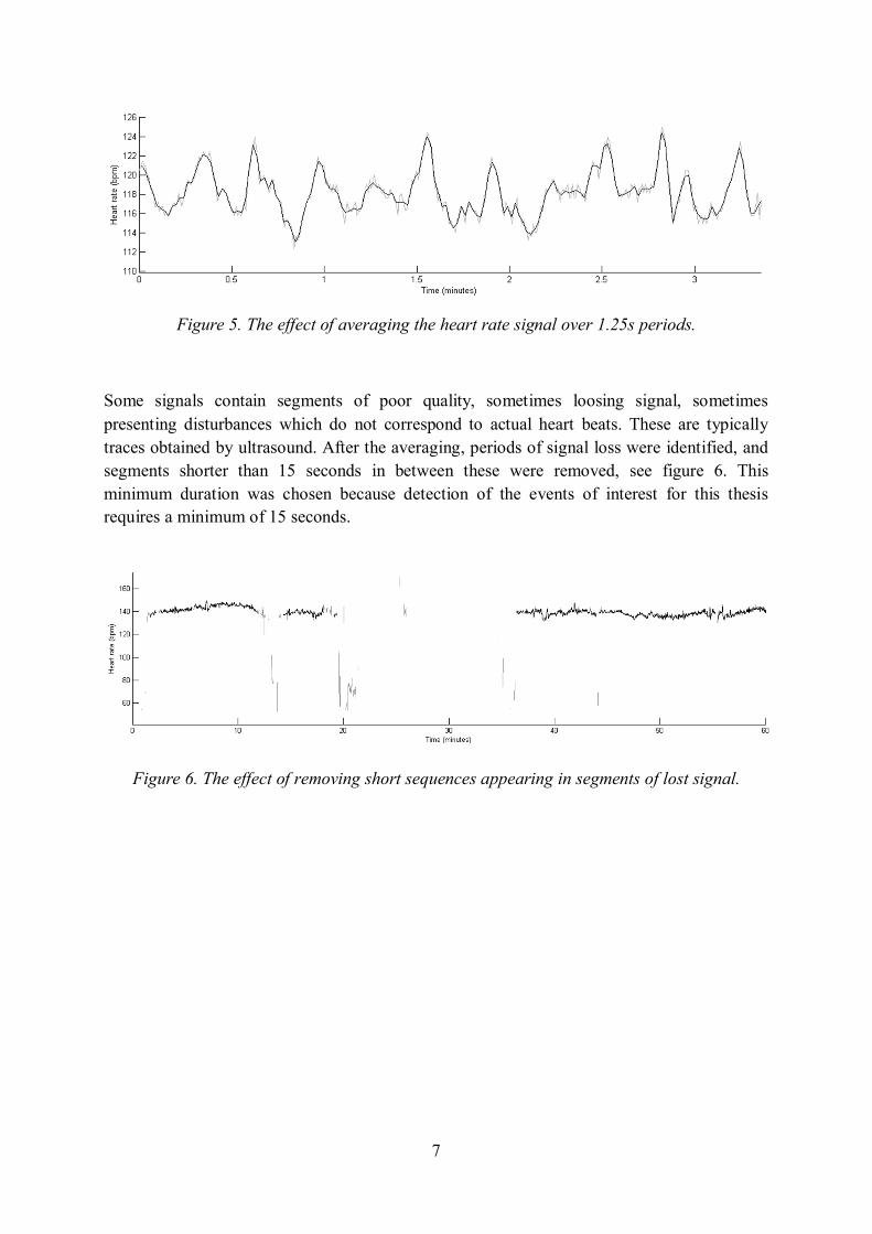
For this thesis a sampling duration of 1.25 seconds, 0.8 Hz, was chosen, see figure 5. This compromise yields acceptable processing time but also adequate signal quality not seriously distorting the acceleration and deceleration flanks. With this sampling period, consecutive samples can also constitute multiples of five seconds.

7

Figure 5. The effect of averaging the heart rate signal over 1.25s periods.

Some signals contain segments of poor quality, sometimes loosing signal, sometimes presenting disturbances which do not correspond to actual heart beats. These are typically traces obtained by ultrasound. After the averaging, periods of signal loss were identified, and segments shorter than 15 seconds in between these were removed, see figure 6. This minimum duration was chosen because detection of the events of interest for this thesis requires a minimum of 15 seconds.

Figure 6. The effect of removing short sequences appearing in segments of lost signal.

8

2.2 Running baseline estimation Accelerations and decelerations are defined as deviations from a running baseline. The running baseline however, is defined as the average fetal heart rate, accelerations and decelerations being excluded. Different methods of estimating the baseline has been suggested (Dawes 1982, Mantel 1990, Ayres-de-Campos 2000). This section describes the development of two algorithms for baseline estimation. Accelerations and decelerations would later be detected as deviations from these running baselines. The clinically implemented algorithm for baseline estimation developed by Dawes et al. is also described.

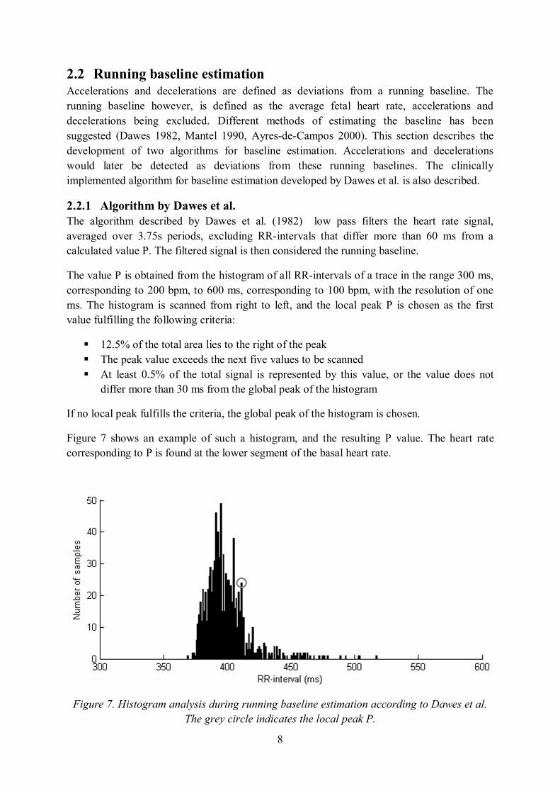
2.2.1 Algorithm by Dawes et al. The algorithm described by Dawes et al. (1982) low pass filters the heart rate signal, averaged over 3.75s periods, excluding RR-intervals that differ more than 60 ms from a calculated value P. The filtered signal is then considered the running baseline.

The value P is obtained from the histogram of all RR-intervals of a trace in the range 300 ms, corresponding to 200 bpm, to 600 ms, corresponding to 100 bpm, with the resolution of one ms. The histogram is scanned from right to left, and the local peak P is chosen as the first value fulfilling the following criteria:

§ 12.5% of the total area lies to the right of the peak § The peak value exceeds the next five values to be scanned § At least 0.5% of the total signal is represented by this value, or the value does not

differ more than 30 ms from the global peak of the histogram

If no local peak fulfills the criteria, the global peak of the histogram is chosen.

Figure 7 shows an example of such a histogram, and the resulting P value. The heart rate corresponding to P is found at the lower segment of the basal heart rate.

Figure 7. Histogram analysis during running baseline estimation according to Dawes et al. The grey circle indicates the local peak P.

9

Dawes et al. initiate the analysis after ten minutes, and if the Dawes/Redman criteria are not met, it continues to recalculate the baseline every two minutes until 60 minutes have passed, always considering the whole heart rate trace.

2.2.2 ModificationofthealgorithmbyDawesetal.Mantel et al. (1990) implemented the procedure for estimating the running baseline described by Dawes et al. for the study of relations between fetal heart rate and fetal movements. The calculated baseline did not correspond to their visual assessment. Hence an improved algorithm was proposed. This improved algorithm was shown to cause less elevations of the baseline in segments of repeated accelerations or large swings of the fetal heart rate. It also showed an improved performance at the beginning of traces. Here, the algorithm described by Dawes et al. fails if the heart rate is declining or inclining, due to that the starting point is an average of the first 64 samples, or four minutes.

Mantel et al. samples an average of the signal each 2.5 seconds, and then use the peak P the same way as Dawes et al. However, after the low pass filtration is completed, the sampled fetal heart rate signal is matched against the filtered version, which could be considered a temporary baseline, and the segments of the signal which deviate too much from this baseline is replaced with the filtered version. This results in a heart rate signal from which the extremes have been trimmed off. The filtration and trimming is repeated four times, removing smaller deviations after each iteration. One last filtration generates the final running baseline. This iterative approach addresses the issue of the baseline being the fetal heart rate when accelerations and decelerations are excluded, while it needs to be defined prior to detecting these events.

The algorithm described by Mantel et al. operates on two-hour long offline registrations, which is also different from the original algorithm.

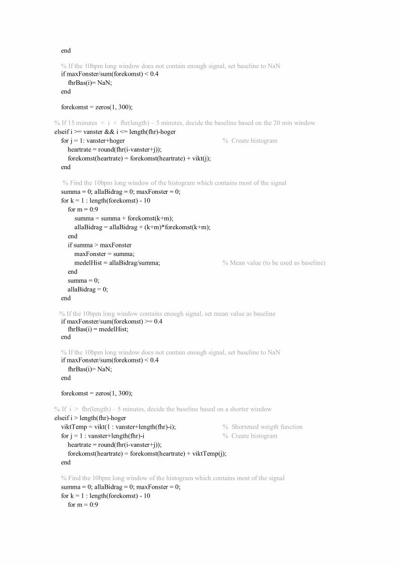
2.2.3 Algorithm1For this thesis, the purpose was to find an algorithm that continues observations for several hours, theoretically for infinite time. Hence, it would not have been suitable to consider the entire signal as in the algorithms proposed by Dawes et al. and Mantel et al. The solution was to apply the baseline estimation on a sliding window, which causes a delay but still is useful, and the resulting algorithm, inspired by Mantel et al., is labeled algorithm 1. The size of the window was set to 20 minutes, since 20 minutes is considered minimum for CTG assessment (Neoventa Medical AB 2008).

Low pass filtering suppresses high frequency components, such as the short time fluctuations, giving a smooth signal. Accelerations and decelerations do however contain very low frequency components on which the filter has little effect, causing the calculated baseline to follow the large deviations from baseline. Therefore, Mantel et al, as well as Dawes et al, exclude all RR-interval deviations of 60 ms or more from P during baseline estimation. This value is calculated based on the histogram of the entire heart rate signal being analyzed. Directly implemented into the 20 minute window, and tested on the traces collected for this thesis, P was not always perfectly chosen. Partly because using a small window, P becomes

10

more locally estimated and therefore follow elevations in the heart rate trace to a greater extent, but also because the algorithms described by Dawes et al. and Mantel et al. was both developed for use on antepartum traces, and hence not prepared for the frequent, heavy decelerations seen in the intrapartum traces.

The filter used in algorithm 1 is a smoothing filter with forward and backward propagation. A pliable enough baseline, which still do not follow accelerations and decelerations entirely, were established through trial and error. The signal B is processed at each sample i according to

Bi = 0.975Bi-1 + 0.025Bi in forward propagation Bi = 0.975Bi+1 + 0.025Bi in backward propagation

where each sample corresponds to a 1.25 second long interval.

P is used to determine an initial value for the filtration in the algorithm described by Mantel et al. A pretended heart rate for the time prior to the actual start of the signal is calculated by starting with the value P, scanning the signal in backward direction, and gradually adjusting the starting value as a function of the signal contributions.

The same approach was adopted for algorithm 1, starting with the value B0 = P, the signal was scanned in backward direction and the starting value B0 was updated at each sample i according to

B0 = 0.975B0 + 0.025Bi

The choice of B0 = P prior to the initial value estimation will have minimal influence on the final B0.

For this thesis, P was not considered as useful as it was for Mantel et al. because of the large influence of local events of the signal. However, since it was already calculated to aid in estimating a starting value, the criteria of deviations from P was not removed entirely but instead modified to only exclude the extremely large decelerations, causing most damage on the filtered signal. Experiments led to a limitation where heart rates exceeding P ± 50 bpm were excluded.

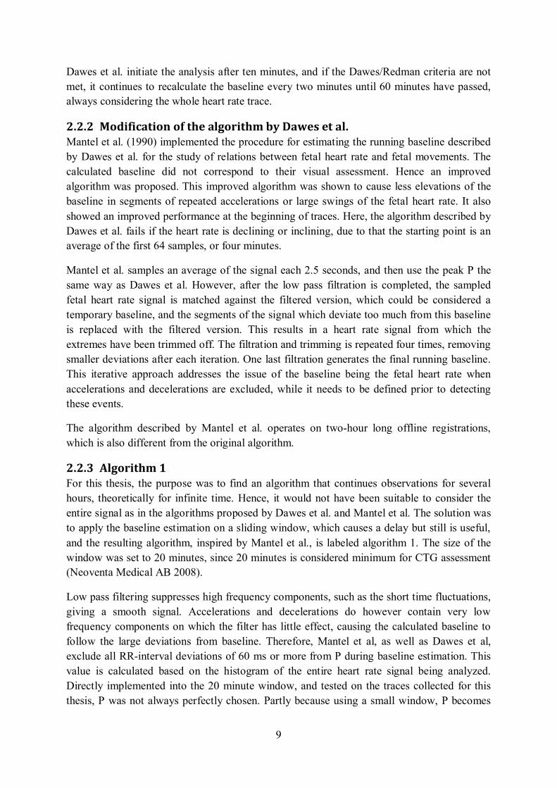
Replacement of segments in the heart rate signal, performed after each iteration of filtering, was done on sequences which deviated too much from the filtered signal, which can be considered a temporary baseline. These segments were replaced by the filtered version from the point where the deviation from the baseline started, to the return to baseline. Thresholds for which deviations to remove are seen in tables 1 and 2. Mantel et al. chose to preserve more deviating heart rate signal below the temporary baseline than what is proposed in this thesis. They justify this as a compensation for selecting P, which was used for limiting the operation range of the filter, in the lower segment of the baseline. Directly implemented into algorithm 1, where P is used differently and on intrapartum traces, the thresholds proposed by Mantel et al. caused the baseline to follow deep or frequent decelerations. Hence different

11

variations of these thresholds were tested. The ones proposed in table 2 performed best on the given intrapartum traces, and was chosen for algorithm 1.

Upper and lower limits by Mantel et al. Iteration Upper limit [bpm] Lower limit [bpm]

1 20 20 2 15 20 3 10 20 4 5 20

Table 1. Detection levels for accelerative and decelerative parts, proposed by Mantel et al.

Upper and lower limits by author Iteration Upper limit [bpm] Lower limit [bpm]

1 20 20 2 15 15 3 10 10 4 5 10

Table 2. Detection levels for accelerative and decelerative parts, proposed for algorithm 1.

Figure 8 presents an example of the temporary baseline updated after each iteration of filtration and replacement of the accelerative and decelerative segments in the heart rate trace.

12

Figure 8. Four iterations of filtration and trimming followed by one last filtration.

13

The window used to mimic real time was set to 20 minutes. Initial experiments were performed calculating the baseline corresponding to a specific sample based on the previous 20 minutes. This resulted in a delayed baseline, which also followed accelerations and decelerations rather than replacing these segments with preliminary baseline. It was necessary to study some future values. The window was changed to 15 minutes of previous and five minutes of future values. Hence, the proposed algorithm causes a delay in analysis of five minutes.

The resulting running baseline is a smooth signal which does not change much between adjacent samples. For speed of analysis the baseline is not updated for each new sample. Instead, a new calculation is performed each minute. It estimates the baseline based on the heart rates within the whole 20 minute window, however only stores 1 minute of the resulting baseline.

Figure 9 shows an example of the issues arising during periods of frequent decelerations, where contributions from lower deceleration heart rates are just as dominant as the baseline heart rates sought. This is typical for the late intrapartum traces.

Figure 9. Both graphs correspond to the same trace. Notice the difference in time scale. The running baseline is affected by contributions from deep and frequent decelerations.

14

2.2.4 Algorithm 2 The previously proposed algorithm encounters obstacles when segments of frequent decelerations occur. Therefore, an alternative approach to estimate a running baseline has been developed with the main purpose of overcoming these issues. Rather than using smoothing filters for estimating the baseline, the histogram of the heart rate signal is studied.

For each new sample of the heart rate signal a histogram is calculated. The histogram represents the fetal heart rates present within the 20 minute window, of 15 previous and five future minutes. The heart rates are weighted into the histogram according to the weight function w(t) seen below and in figure 10. This causes current heart rate to have higher effect on the histogram than previous or future heart rates.

( ) =( ) , ∈ {0, 15}, ( ) ∈ {0, 5}

( ) , ∈ {15, 20}, ( ) ∈ {2, 0.1}0, ℎ

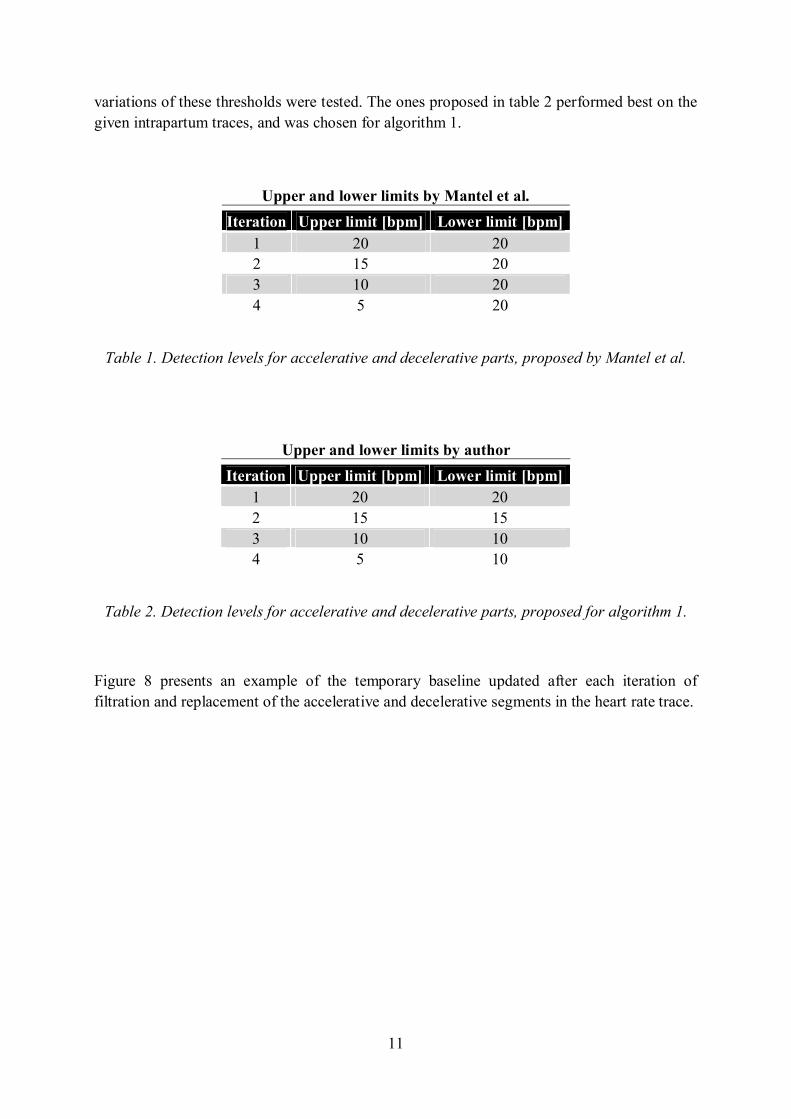
After the histogram has been calculated it is scanned to find the ten bpm wide window which carries the most of the heart rate signal, see figure 11, to find a plausible estimate for the baseline. The mean value of the contributions within this window is chosen as baseline for this particular sample.

The choice of weight function is based on empirical studies, and the parameters were adjusted to obtain the best algorithm performance. Using no weight function, or a flatter one, results in a flatter, less pliable baseline. A sharper weight function, or a shorter window, results in a baseline more prone to shifting during accelerations and decelerations, which was what was aimed to avoid using this method. As concluded when developing algorithm 1, estimating the running baseline based only on previous heart rate values causes a delayed baseline, hence the 15 + five minute window was again chosen.

Figure 10. Function used to weight fetal heart rate contributions into the histogram.

15

Figure 11. Weighted histogram analysis for algorithm 2. The ten bpm wide window carrying most of the signal was 149 – 158 bpm, and the

mean value of the contributions within that span was calculated to 153.50 bpm.

The resulting running baseline from applying this method is seen in figure 12. Finding the most contributing heart rates, rather than using a smoothing filter, gives a sharper baseline which is not centered between deceleration minimums and true baseline level, as the baseline estimated using algorithm 1. This gives a running baseline which handles sections of frequent decelerations better, but which in general looks sharp and quite flat. The figure displays the same trace as the one shown in figure 9, for algorithm 1.

Figure 12. Both graphs correspond to the same trace. Notice the difference in time scale.

The baseline is not as affected by contributions from deep and frequent decelerations, as the baseline calculated by algorithm 1.

16

2.3 Acceleration detection Assuming that the running baseline has been perfectly estimated, all accelerations should easily be detected using the definition described in the introduction.

The running baseline was however not perfectly estimated. Algorithm 2 gives a running baseline which might not be considered pliable enough, and algorithm 1 gives a baseline which does not handle turbulent areas well. Since algorithm 2 detects these critical sections, studying the histogram used in this algorithm was considered a way to measure the reliability of any calculated baseline. In the case of accelerations, one would rather want to fail to detect some than over detect false accelerations. For this reason the calculated baseline could be assessed as unreliable for certain segments using the histogram analysis from algorithm 2, and accelerations should not be sought in these segments. If most of the signal values are found within the ten bpm wide window the baseline would be considered reliable, however if the histogram is a flat shape and not much of the total signal is found within the ten bpm wide window, the baseline would be considered unreliable, hence no accelerations are detected in that segment.

This approach can be applied to any baseline algorithm for acceleration detection. It was implemented on both algorithm 1 and algorithm 2. The amount of signal found in the ten bpm wide window was expressed as a percentage of the total histogram, and the traces for testing were run through the two algorithms, varying this parameter with the purpose of finding the acceleration detection performance which best matched the one between the expert observers.

2.4 Deceleration detection The approach of rejecting segments of unreliable baseline, tested for acceleration detection, was not relevant for deceleration detection since most of the disregarded baseline segment were neglected because of decelerations. Instead, to find the performances which best matched the one between the expert observers, the test traces for deceleration detection were run through the algorithms varying the different minimum required time duration of decelerations, and the minimum required excursion from the baseline.

2.5 Basal heart rate While the running baseline used for detecting accelerations and decelerations follow the trace influenced by minor elevations, the basal heart rate is expressed as only one value rounded to multiples of five. Basal heart rate is expressed in bpm and values between 110 bpm and 160 bpm are considered normal (Macones 2008).

This section describes two proposed algorithms for basal heart rate estimation. The clinically implemented algorithms for baseline estimation developed by Dawes et al. and Ayres-de-Campos et al. respectively are also described.

During development the algorithms for basal heart rate estimation were applied to the 20 minutes long traces for which observer 1 determined a basal heart rate.

17

2.5.1 Algorithms by Dawes et al. and Ayres-de-Campos et al. Dawes et al. (1982) define the basal heart rate as the average fetal heart rate during episodes of low variation. Low variation is defined by a maximum excursion from the baseline of less than 30 ms for five out of six consecutive one-minute segments. If the trace does not contain any episodes of low variation, the local peak value P, calculated during baseline estimation in section 2.2.1, is selected as basal heart rate.

The algorithm developed by Ayres-de-Campos et al. (2000) is based on histogram analysis. It selects a few highly represented heart rates from the signal. Based on these and short term variability analysis a basal heart rate is determined from the lowest heart rate within physiological limits where a stable segment is found. The algorithm is complex and its flow chart can be found in appendix F.

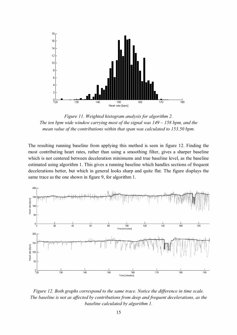
2.5.2 Algorithm A The algorithm is based on histogram analysis of the fetal heart rate trace. All heart rates are rounded to multiples of five into a histogram. The mode of the histogram is then chosen as the basal heart rate. In the example shown in figure 13, with corresponding histogram in figure 14, the mode 145 bpm was chosen as the basal heart rate. Observer 1 however, estimated the basal heart rate as 150 bpm.

Figure 13. Fetal heart rate trace on which algorithm A has been applied. The algorithm estimated the basal heart rate as 145 bpm. Observer 1 however estimated it as 150 bpm.

Figure 14. Corresponding histogram analysis of fetal heart rate trace, used for algorithm A.

18

2.5.3 Algorithm B This algorithm is a modification of algorithm A. Basal heart rate should by definition only be sought in stable segments. The algorithm therefore, prior to histogram analysis, removes segments from the fetal heart rate signal which are not considered stable segments. The same criterion for identifying stable segments is used as during preprocessing of the heart rate signal, five subsequent samples not differing more than ten bpm. With this approach, much of the accelerations and decelerations are removed from the signal.

All heart rates are rounded to multiples of five into a histogram. The mode of the histogram is then chosen as the basal heart rate.

Figure 15 shows a heart rate trace on which algorithm B has been applied. It is the same heart rate trace as shown for algorithm A. The dark lines represent the stable segments on which histogram analysis has been performed. Figure 16 shows the histogram. In this example, the mode 150 bpm was chosen as the basal heart rate. This matches the estimation made by observer 1.

Figure 15. Fetal heart rate trace on which algorithm B has been applied. Dark lines represent the stable segments on which histogram analysis was performed. The estimated basal heart rate, 150 bpm, matches the estimation made by observer 1.

Figure 16. Corresponding histogram analysis of fetal heart rate trace, used for algorithm B.

19

2.5.4 Undefined by expert observer Observer 1 marked the basal heart rate as ‘undefined’ in ten of the 50 test traces. Ideally, an algorithm for basal heart rate estimation would do the same. Experiments were carried out aiming to find correlations between these traces. Possible correlations were sought in the signal loss, defined as the fraction of resampled intervals which did not contain a heart rate value after the preprocessing, i.e. they either did not contain a value prior to preprocessing, or the RR-intervals were considered as artifacts and removed. Figure 17 shows the signal loss expressed in percentage of the total signal.

Figure 17. Signal loss in the test traces for which observer 1 estimated a basal heart rate, compared to those which were marked ‘undefined’.

The signal loss parameter can clearly be used to identify some of the traces where the basal heart rates were assessed as undefined. Based on this set of data a threshold for allowed signal loss was set to 65%, which captured three of the traces. The criterion was applied to both algorithm A and algorithm B.

20

3. Results This section presents the results from the inter-observer agreement study, testing of the developed algorithms, as well as validation of the developed algorithms.

3.1 Acceleration detection

3.1.1 Observer uncertainty Both observer 1 and observer 2 marked the time intervals for which accelerations occur for the validation traces. The performance of observer 2 against observer 1 on the validation data is seen in table 3.

The program written to evaluate sensitivity and positive predictive value for acceleration and deceleration detection in this thesis regards an event as correctly detected when overlap is found in time intervals marked by both observer 1 and the algorithm or observer 2.

Observer uncertainty: acceleration detection Sensitivity 0.852

Positive predictive value 0.377

Table 3. Acceleration detection by observer 2, against observer 1.

3.1.2 Testing The test traces were run through the two proposed algorithms for acceleration detection, as well as the algorithm described by Dawes et al. for performance comparison, against the opinions of observer 1. The parameter defining the baseline as not valid was varied with the purpose of finding the best performance to match the accuracy of the observers, see figure 18. The right part of the graph shows results from when all baseline is accepted. Results towards the left correspond to rejecting large segments of the baseline, including all larger accelerations as they provide wide distribution in the histogram. Notice that the performance by observer 2 correspond to the results from running the set of traces for validation, not the ones for training. One cannot know for certain that the test data and validation data yields the same results, although it is desired.

The Dawes/Redman criteria define acceleration as lasting for a minimum of ten seconds instead of 15 seconds used for the other algorithms. This results in an increased detection rate, at the expense of low positive predictive value.

21

Figure 18. Acceleration detection based on baseline estimation according to algorithm 1, algorithm 2 and the algorithm by Dawes et al. The baseline rejecting parameter is varied.

Performances are evaluated against opinions of observer 1. The square indicates the performance of observer 2.

The positive predictive value or the sensitivity never reached 1 when altering this parameter. The sensitivity never did so because all portions of the baseline were considered valid and the algorithms cannot perform better than this. The positive predictive value never did so because some detected accelerations did not coincide with an acceleration marked by the observer. This might be explained as either poor baseline estimation or poor adaption of the definition of acceleration by the observer.

Defining which baseline segments to reject is a matter of deciding whether one seeks to detect all accelerations, and thereby greatly over detect, or failing to detect a large group of accelerations, however with high certainty of the ones detected. By performing validation on the parameters resulting in performance in the same positive predictive value area as observer 2, the performance could be compared fairly by studying the corresponding sensitivity. Hence, the parameters resulting in positive predictive value 0.39 (algorithm 1) and 0.38 (algorithm 2) was chosen to match 0.38 (observer 2). This was realized by allowing a minimum of 40% of the total histogram within the ten bpm wide window.

22

3.1.3 Validation The traces for validation were run through the two proposed algorithms, with the baseline rejecting parameters adjusted as described. See figure 19. Here, the performance by observer 2 indicated in the graph correspond to the same data set as for the algorithms. Ideally performance on the validation data would be exactly the same as on the test data. These results show that the algorithms follow the expected curves obtained from testing, however with lower sensitivity than expected, and that observer 2 better matches the opinions of observer 1 than the algorithms do in terms of sensitivity.

Figure 19. Validation of acceleration detection based on baseline estimation according to algorithm 1 and algorithm 2.


23

3.2 Deceleration detection

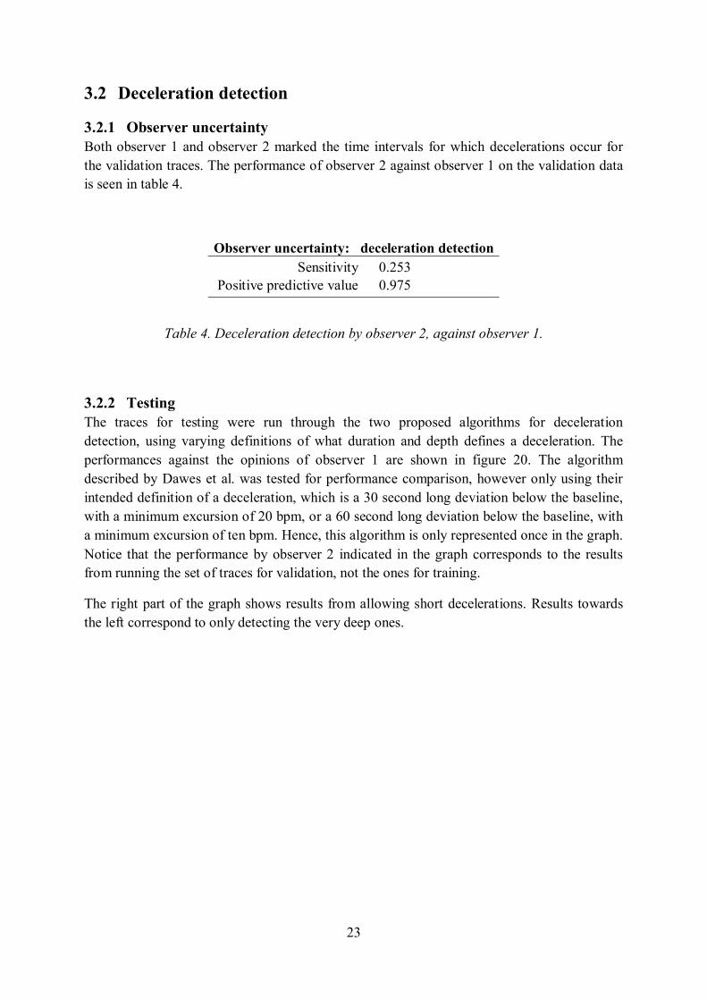
3.2.1 Observer uncertainty Both observer 1 and observer 2 marked the time intervals for which decelerations occur for the validation traces. The performance of observer 2 against observer 1 on the validation data is seen in table 4.

Observer uncertainty: deceleration detection Sensitivity 0.253

Positive predictive value 0.975

Table 4. Deceleration detection by observer 2, against observer 1.

3.2.2 Testing The traces for testing were run through the two proposed algorithms for deceleration detection, using varying definitions of what duration and depth defines a deceleration. The performances against the opinions of observer 1 are shown in figure 20. The algorithm described by Dawes et al. was tested for performance comparison, however only using their intended definition of a deceleration, which is a 30 second long deviation below the baseline, with a minimum excursion of 20 bpm, or a 60 second long deviation below the baseline, with a minimum excursion of ten bpm. Hence, this algorithm is only represented once in the graph. Notice that the performance by observer 2 indicated in the graph corresponds to the results from running the set of traces for validation, not the ones for training.

The right part of the graph shows results from allowing short decelerations. Results towards the left correspond to only detecting the very deep ones.

24

Figure 20. Deceleration detection based on baseline estimation according to algorithm 1 and algorithm 2, for five, ten and 15 seconds duration required for deceleration detection.

The minimum excursion from baseline required for deceleration detection is varied. Performances are evaluated against opinions of observer 1.

The square indicates the performance of observer 2 The circle indicates the performance of the algorithm by Dawes et al.

Testing of the developed algorithms shows that defining the depth of a deceleration as five, ten or 15 bpm below the baseline does not affect the sensitivity significantly. These minimum excursions from the baseline are represented in the graph as the three indicators at the extreme right of each curve. This justifies that the clinical experts did define decelerations only with an excursion from baseline of 15 bpm or more. The parameter does however have a great impact on the positive predictive value since false decelerations are more frequently detected when the detection limits are lowered. Hence, defining the minimum excursion from the baseline of a deceleration as five bpm or ten bpm is not recommended. Setting this parameter to 20 bpm yields nearly the same positive predictive value as obtained from the algorithm described by Dawes et al. When decelerations are defined as deeper than this the duration no longer matters for the detection. At this depth, there were no decelerations marked by observer 1 shorter than 15 seconds.

Sensitivity or positive predictive value never reached 1 when altering these parameters. Deceleration detection on five seconds long deviations of only five bpm from the baseline still did not yield full sensitivity against observer 1. This indicates disagreement in the running baseline estimation.

25

The inter-observer performance is found in a region of high positive predictive value and quite low sensitivity. It is a probable assumption that mainly deep decelerations have been detected. It makes no difference if validation is performed on five, ten or 15 seconds duration, since these yield the same results. Deceleration detection of 15 seconds long deviations were however chosen for validation, because of accordance with guideline definition.

Validation was performed using the parameters which resulted in positive predictive value 0.953 (algorithm 1) and 0.967 (algorithm 2), in order to match 0.975 (observer 2). This was realized by detecting 15 seconds long segments, with minimum excursion of 40 bpm (algorithm 1) and 50 bpm (algorithm 2) below the baseline.

3.2.3 Validation The traces for validation were run through the two proposed algorithms, with the depth and duration parameters adjusted as described, see figure 21. Here, the performance by observer 2 indicated in the graph correspond to the same data set as for the algorithms. The results show that both algorithms follow the expected curves obtained from testing, and that they imitate observer 1 with higher accuracy than observer 2 does.

Figure 21. Validation of deceleration detection based on baseline estimation according to algorithm 1 and algorithm 2.


26

3.3 Basal heart rate

3.3.1 Observer uncertainty Both observer 1 and observer 2 estimated the basal heart rate for the validation traces. The performance of observer 2 against observer 1 on the validation data is seen in table 5.

Observer uncertainty: basal heart rate estimation

Difference [bpm] Occurences [%] 0 72 5 10 10 2 > 10 2

Undefined only by observer 1 0

Undefined only by observer 2 16

Table 5. Basal heart rate estimation by observer 2, against observer 1.

3.3.2 Testing The traces for testing were run through the proposed algorithms for basal heart rate estimation. The performances against the opinions of observer 1 are shown in figure 22. The algorithms described by Dawes et al. and Ayres-De-Campos et al. were tested for performance comparison.

The two observers, as well as the proposed algorithms, round the basal heart rates to multiples of five. The algorithms described by Dawes et al. and Ayres-De-Campos et al. however do not. For a fair comparison, the results from these two algorithms have been rounded to the nearest multiple of five.

Figure 22. Performance against observer 1 for basal heart rate estimation.

27

The results indicate that excluding unstable segments from the heart rate signal prior to estimating the basal heart rate using histogram analysis result in higher accuracy. Hence, algorithm B was chosen for validation.

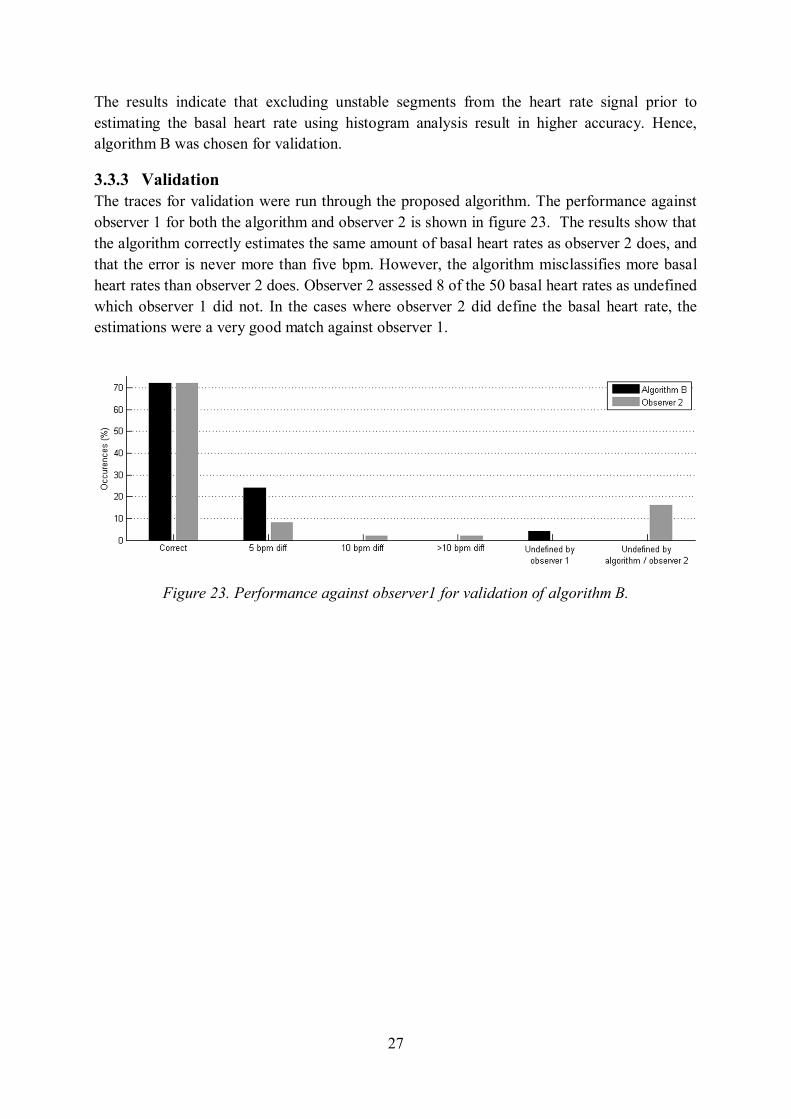
3.3.3 Validation The traces for validation were run through the proposed algorithm. The performance against observer 1 for both the algorithm and observer 2 is shown in figure 23. The results show that the algorithm correctly estimates the same amount of basal heart rates as observer 2 does, and that the error is never more than five bpm. However, the algorithm misclassifies more basal heart rates than observer 2 does. Observer 2 assessed 8 of the 50 basal heart rates as undefined which observer 1 did not. In the cases where observer 2 did define the basal heart rate, the estimations were a very good match against observer 1.

Figure 23. Performance against observer1 for validation of algorithm B.

28

4. Discussion Identifying fetal hypoxia is a question of correctly interpreting the levels and changes in the fetal heart rate. Indistinct definition of the cardiotocographic events makes this subjective and it has repeatedly been proven poorly reproducible. A great number of previous studies have reported both on poor inter-observer agreement, where interpretation of tracings have shown to differ between clinicians, as well as poor intra-observer agreement, where interpretation by the same clinician at two different occasions differ (Beaulieu 1982, Bernardes 1997, Ayres-de-Campos 1999, Devane 2005, Chauhan 2008, Westerhuis 2009).

Most of the conducted studies deal with the agreement when classifying the CTG as a whole, as more or less reassuring. Hence, they provide no exact information on agreement on baseline estimation, accelerations or decelerations. Results from these studies cannot be compared directly because of inconsistent conditions such as classification categories, number of expert observers, number of cardiotocograms observed and statistical methods used for representing the results. However, inter-observer agreement when classifying overall CTG tracings have been proven poor by Beaulieu (1982), Ayres-de-Campos (1999), Chauhan (2008) and Westerhuis (2009) and intra-observer agreement have been reported poor by Westerhuis (2009). Agreement is generally higher for the tracings classified as normal (Ayres-de-Campos 1999, Chauhan 2008, Westerhuis 2009), and also for antepartum rather than intrapartum tracings (Ayres-de-Campos 99). These two are probably related, since intrapartum tracings contain more periodic changes in the fetal heart rate resulting from uterine contractions.

Results reported from studies where the agreement of baseline heart rate, baseline variability, accelerations and decelerations are compared separately suggest low inter-observer agreement for all variables assessed (Trimbos 1978, Lotgering 1982, Bernardes 1997). All three find baseline heart rate to be the most reproducible, and baseline variability to be the least. Trimbos (1978) found the agreement to be lower for accelerations than decelerations, while on the contrary, Bernardes (1997) found the agreement to be acceptable for accelerations only when the variability was good, but poor otherwise, and always poor for detection of decelerations.

The inter-observer analysis presented in this thesis is in accordance with previous studies, showing considerable disagreement. The lack of observer agreement when analyzing the CTG impairs the credibility of individual visual interpretation, hence questioning decision-making solely based on visual analysis of the fetal heart rate trace. Systematic computer analysis of the CTG is mostlikely the only way to overcome these issues and achieve fully reproducible analysis.

Teaching a computer system how to assess a CTG is however difficult since there is no absolute indicator of fetal hypoxia. The cardiotocographic events indicating this have to be defined based on a nearly consistent agreement by experienced clinicians. Such a consensus is obviously difficult to reach. Definitions have been suggested (Macones 2008), however the interdependence of the baseline definition and the acceleration and deceleration definitions makes direct implementation impossible.

29

Different methods for estimating a running baseline for acceleration and deceleration detection have been suggested. In this thesis, the one most commonly clinically implemented, developed by Dawes et al. (1982) has been compared to two algorithms suggested by the author. Algorithm 1 gives a running baseline which is smooth and pliable. Algorithm 2 gives a shaper baseline which handles frequent and large decelerations better.

4.1 Acceleration and deceleration detection Detection of accelerations and decelerations was implemented into both algorithms by identifying deviations from the running baselines. The two developed algorithms showed very similar results for acceleration detection during the testing phase. Algorithm 2 however, performed with higher sensitivity against the opinions of observer 1 during validation, for nearly the same positive predictive value. None of the algorithms detected the accelerations marked by observer 1 with the same accuracy in terms of sensitivity as observer 2 did. One could apply the same approach to the acceleration detection as was done for deceleration detection, i.e. testing which duration and minimum excursion from the baseline result in best performance. This might increase accuracy against the inter-observer performance slightly. However, increasing sensitivity probably affect the positive predictive value negatively, detecting more false accelerations.

The algorithm described by Dawes et al. succeeded to match the sensitivity of the opinions of observer 1 as observer 2 did, however with very poor positive predictive value. The reason why the detection rate is higher for this algorithm is because it defines an acceleration as lasting for a minimum of ten seconds instead of 15 seconds used by the other algorithms.

Algorithm 2 showed slightly better performance against the opinions of observer 1 than algorithm 1 did for deceleration detection during the testing phase. However algorithm 1 performed better during validation. Both algorithms performed well over all, detecting the decelerations marked by observer 1 with higher accuracy than observer 2 did, both in terms of sensitivity and positive predictive value. The algorithm described by Dawes et al. failed on both aspects. The poor performance of this algorithm might be explained by different causes, one being that the running baseline was developed for antepartum traces, not handling frequent decelerations well. The long averaging period of 3.75 seconds might also imply missed decelerations. A true deceleration might, by this algorithm, be interpreted as a few seconds shorter in duration than it really is. The long averaging period might also imply a risk of not distinguishing between two closely adjacent decelerations.

The definition for deceleration depth applied during validation, 40 bpm for algorithm 1 and 50 bpm for algorithm 2, is extreme. It was chosen to match the inter-observer positive predictive value of observer 2 against the opinions of observer 1, however the results from validation showed better performance by the two algorithms than what was expected from testing. It implies that we might get an accuracy close to that of observer 2 in terms of positive predictive value by allowing smaller decelerations, probably giving much better sensitivity.

30

One explanation for the large difference in performance between acceleration detection and deceleration detection might be that most decelerations were very deep, in contrast to the accelerations which were often close to the definition of a 15 bpm excursion from the baseline, making the accuracy of baseline estimation more crucial.

4.1.1 Alternative methods Unsuccessful efforts were made to find methods to detect accelerations not solely based on duration and excursion from the running baseline.

An algorithm was devolved to detect possible candidate sequences, which on the test data would cause a sensitivity of 1, but a positive predictive value of only 0.16. This was realized by detecting the sequences using very kind definitions in terms of time duration and excursion from the running baseline. Each candidate sequence would then undergo further experiments to be assessed as acceleration or not acceleration. This was realized using a machine learning technique called binary support vector machines, which assigns unseen data to one of two possible classes based on its characteristics, comparing them to previous observations of training sequences which the machine has learned on (Warrick 2010).

Each possible candidate sequence is described as a vector of numerical parameters, the so called ‘features’ of the sequence. These features would describe morphological, statistical, time or frequency domain characteristics, and they should be chosen such that they maximize the difference between the sequences which are true accelerations and those which are false accelerations. The program is trained with such sequences and also informed of the outcome, i.e. if they have been identified as acceleration or not by observer 1. It distributes these into a space where a boundary is found between the two classes, see an example in figure 24. This training is only performed once, after that the binary support vector machine can assign any given data expressed as a feature vector to one of the two classes.

Figure 24. Classification of three dimensional data (i.e. described by three different features characteristics) into two classes (Axelberg 2007).

31

Unfortunately, defining a good set of features was difficult for this application. No tested combination of individual characteristics separated the true accelerations from the false accelerations. Around 30 different features, and different combinations of these, were tested. Examples of these were:

§ Time duration for which the heart rate exceed various levels § Size of the excursion from baseline § Standard deviation § Entropy § Rise time and recovery time § Gradient at onset and recovery § Matching of the sequence against desired functions § Characteristics based on wavelet analysis § Coefficients from discrete cosine transform, as proposed by Warrick et al (2005)

The best results were found to be obtained using features related to time duration of the sequence and the size of its excursion from the running baseline, which makes this detour quite uncalled for. Testing showed sensitivity of 0.52 and a positive predictive value of 0.30 which is worse performance than both algorithm 1 and algorithm 2, and about the same as the performance of the algorithm described by Dawes et al.

During discussion with the expert observers around this time it was revealed that their assessment of accelerations and decelerations were indeed based solely on fitting a running baseline, and then identifying the events based on the definitions. Their believes are that there are no other parameters involved, hence this method was not further evaluated.

4.1.2 Impact of observer uncertainty The interagreement study in this thesis, for acceleration detection, reported that observer 2 matched the opinions of observer 1 with a positive predictive value of only 0.377, and a sensitivity of 0.852. However, if the opposite comparison is made, observer 1 matches the opinions of observer 2 with a positive predictive value of 0.852 and a sensitivity of 0.377.

Because observer 2 only assessed the CTG traces to be used for validation, and not the ones used for development and testing, the algorithms for acceleration and deceleration detection were developed to match the opinions of observer 1. However, it might be of interest to see how well the developed algorithms actually perform against observer 2.

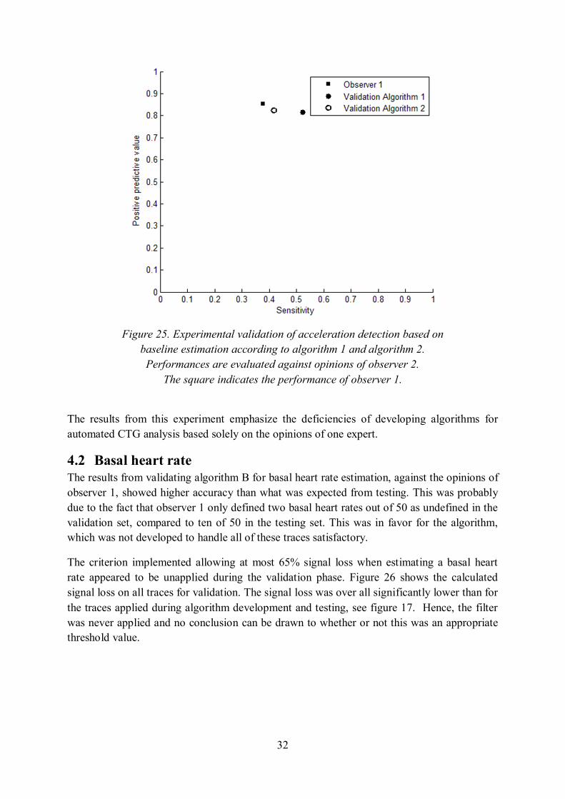
Figure 25 shows that results from experimental validation against the opinions of observer 2 instead of observer 1 gives much better performance by the algorithms, even though they have been developed aiming to match the opinions of observer 1. The results show higher sensitivity than the inter-observer performance, for nearly the same positive predictive value. Presumably, the performance could have been even better if test data from observer 2, which was not available, was used during development, and of course if the parameters chosen for validation was based on a comparison against observer 2 instead of observer 1.

32

Figure 25. Experimental validation of acceleration detection based on baseline estimation according to algorithm 1 and algorithm 2.


The results from this experiment emphasize the deficiencies of developing algorithms for automated CTG analysis based solely on the opinions of one expert.

4.2 Basal heart rate The results from validating algorithm B for basal heart rate estimation, against the opinions of observer 1, showed higher accuracy than what was expected from testing. This was probably due to the fact that observer 1 only defined two basal heart rates out of 50 as undefined in the validation set, compared to ten of 50 in the testing set. This was in favor for the algorithm, which was not developed to handle all of these traces satisfactory.

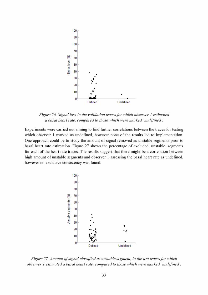
The criterion implemented allowing at most 65% signal loss when estimating a basal heart rate appeared to be unapplied during the validation phase. Figure 26 shows the calculated signal loss on all traces for validation. The signal loss was over all significantly lower than for the traces applied during algorithm development and testing, see figure 17. Hence, the filter was never applied and no conclusion can be drawn to whether or not this was an appropriate threshold value.

33

Figure 26. Signal loss in the validation traces for which observer 1 estimated a basal heart rate, compared to those which were marked ‘undefined’.

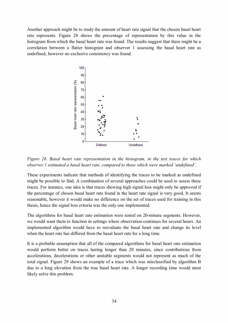
Experiments were carried out aiming to find further correlations between the traces for testing which observer 1 marked as undefined, however none of the results led to implementation. One approach could be to study the amount of signal removed as unstable segments prior to basal heart rate estimation. Figure 27 shows the percentage of excluded, unstable, segments for each of the heart rate traces. The results suggest that there might be a correlation between high amount of unstable segments and observer 1 assessing the basal heart rate as undefined, however no exclusive consistency was found.

Figure 27. Amount of signal classified as unstable segment, in the test traces for which observer 1 estimated a basal heart rate, compared to those which were marked ‘undefined’.

34

Another approach might be to study the amount of heart rate signal that the chosen basal heart rate represents. Figure 28 shows the percentage of representation by this value in the histogram from which the basal heart rate was found. The results suggest that there might be a correlation between a flatter histogram and observer 1 assessing the basal heart rate as undefined, however no exclusive consistency was found.

Figure 28. Basal heart rate representation in the histogram, in the test traces for which observer 1 estimated a basal heart rate, compared to those which were marked ‘undefined’.

These experiments indicate that methods of identifying the traces to be marked as undefined might be possible to find. A combination of several approaches could be used to assess these traces. For instance, one idea is that traces showing high signal loss might only be approved if the percentage of chosen basal heart rate found in the heart rate signal is very good. It seems reasonable, however it would make no difference on the set of traces used for training in this thesis, hence the signal loss criteria was the only one implemented.

The algorithms for basal heart rate estimation were tested on 20-minute segments. However, we would want them to function in settings where observation continues for several hours. An implemented algorithm would have to reevaluate the basal heart rate and change its level when the heart rate has differed from the basal heart rate for a long time.

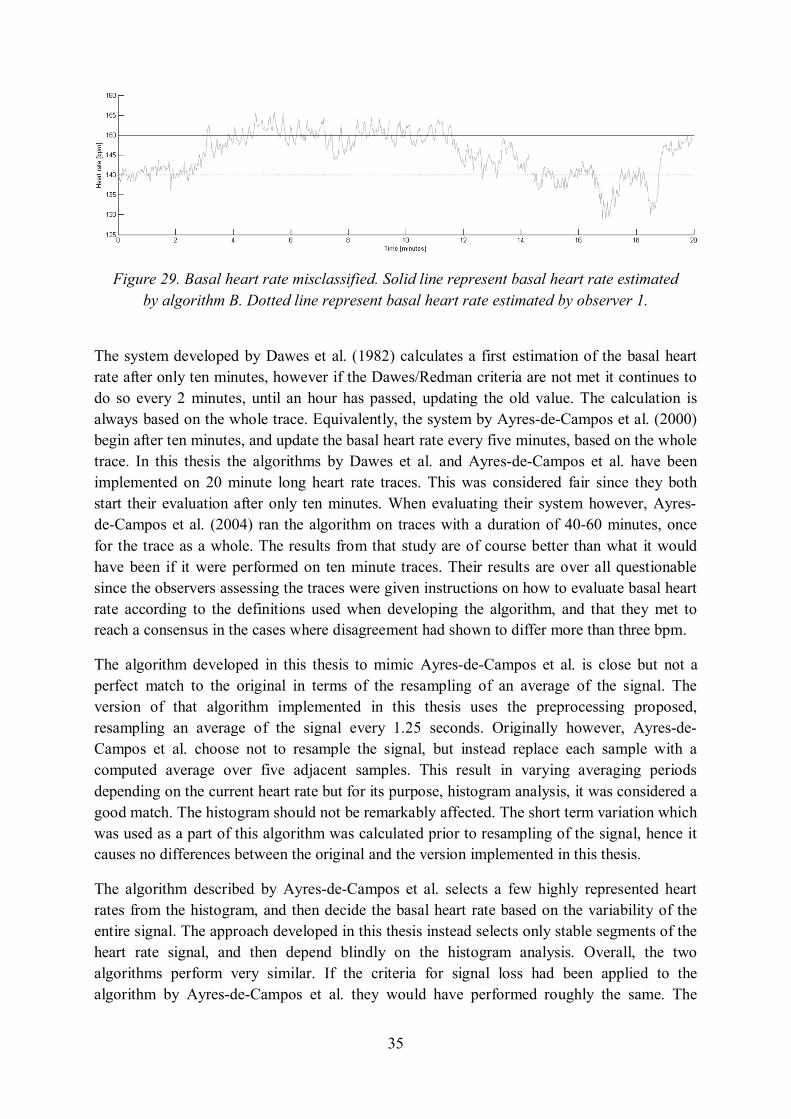
It is a probable assumption that all of the compared algorithms for basal heart rate estimation would perform better on traces lasting longer than 20 minutes, since contributions from accelerations, decelerations or other unstable segments would not represent as much of the total signal. Figure 29 shows an example of a trace which was misclassified by algorithm B due to a long elevation from the true basal heart rate. A longer recording time would most likely solve this problem.

35

Figure 29. Basal heart rate misclassified. Solid line represent basal heart rate estimated by algorithm B. Dotted line represent basal heart rate estimated by observer 1.

The system developed by Dawes et al. (1982) calculates a first estimation of the basal heart rate after only ten minutes, however if the Dawes/Redman criteria are not met it continues to do so every 2 minutes, until an hour has passed, updating the old value. The calculation is always based on the whole trace. Equivalently, the system by Ayres-de-Campos et al. (2000) begin after ten minutes, and update the basal heart rate every five minutes, based on the whole trace. In this thesis the algorithms by Dawes et al. and Ayres-de-Campos et al. have been implemented on 20 minute long heart rate traces. This was considered fair since they both start their evaluation after only ten minutes. When evaluating their system however, Ayres-de-Campos et al. (2004) ran the algorithm on traces with a duration of 40-60 minutes, once for the trace as a whole. The results from that study are of course better than what it would have been if it were performed on ten minute traces. Their results are over all questionable since the observers assessing the traces were given instructions on how to evaluate basal heart rate according to the definitions used when developing the algorithm, and that they met to reach a consensus in the cases where disagreement had shown to differ more than three bpm.

The algorithm developed in this thesis to mimic Ayres-de-Campos et al. is close but not a perfect match to the original in terms of the resampling of an average of the signal. The version of that algorithm implemented in this thesis uses the preprocessing proposed, resampling an average of the signal every 1.25 seconds. Originally however, Ayres-de-Campos et al. choose not to resample the signal, but instead replace each sample with a computed average over five adjacent samples. This result in varying averaging periods depending on the current heart rate but for its purpose, histogram analysis, it was considered a good match. The histogram should not be remarkably affected. The short term variation which was used as a part of this algorithm was calculated prior to resampling of the signal, hence it causes no differences between the original and the version implemented in this thesis.

The algorithm described by Ayres-de-Campos et al. selects a few highly represented heart rates from the histogram, and then decide the basal heart rate based on the variability of the entire signal. The approach developed in this thesis instead selects only stable segments of the heart rate signal, and then depend blindly on the histogram analysis. Overall, the two algorithms perform very similar. If the criteria for signal loss had been applied to the algorithm by Ayres-de-Campos et al. they would have performed roughly the same. The

36

algorithm described by Dawes et al. however, performs much worse. The reason for this is understandable since it calculates the mean value of the stable segments, instead of the mode. This theoretically means that the calculated value may not even be present in the signal at all. The same approach was tested at an early stage of this project, however on the entire signal, with similar results.

4.3 Gathering of expert observer opinions Clinical expert evaluation of the cardiotocograms was time consuming. For the scope of this thesis, employing two clinical experts to evaluate the registrations was initially considered the realistic alternative. Inter-observer variability was however reported higher than expected, which implied difficulties defining the absolute performance of the developed algorithms. The algorithms described by Dawes et al., which are widely used clinically, perform poor against observer 1 on these heart rate traces. It cannot be fully concluded whether the observer data is extraordinary, or if the algorithms are inadequate. However, the developed algorithms did perform better than the competing algorithms, and within or close to the uncertainty between the clinical experts.

Ideally this study would have been carried out on a larger group of clinical experts, leaving more room for classifying rare opinions as less significant, and more commonly shared opinions as more convincing. With only the sparse information from two observers, there is no statistical significance and more reliable results than those obtained are not possible.

Both observers have assured that they did evaluate the fetal heart rate traces according to the same definitions of acceleration, deceleration and basal heart rate. They believe that the low inter-observer agreement observed for acceleration detection is caused solely by an uncertainty of where to fit the baseline.

The conditions under which the cardiotocograms were assessed by the observers inevitably differed from the typical clinical setting. Evaluation was performed studying the registrations with the same computer software used clinically. They were however studied offline, implying two major factors to their advantage. Firstly, there was almost unlimited time for analysis. The observers could take their time and pause the evaluation whenever they needed to due to distractions. Secondly, unlike a real time setting, the observers were given the whole registration at once, facilitating evaluation of each event by the possibility to study not only previous but also future heart rates. It is not likely that the unusual conditions under which the cardiotocograms were assessed caused poorer judgment. It is more likely that it had a positive effect on the validity of the evaluation.

Ideally validation of an algorithm would give the same results as obtained in the testing stage, proving that the algorithms have been developed to operate on any general data. Validation of acceleration detection, deceleration detection as well as basal heart rate estimation show that there is a difference between results obtained from test data and validation data in this thesis. It is plausible to believe that the observed differences are a result of the small number of cardiotocograms used, and that a larger study would strengthen the certainty of any results.

37

4.4 Clinical impact of the results Accelerations are considered the most important indication of fetal wellbeing (Ingemarsson 2006). It indicates a well functioning cardiovascular system, a functioning autonomic nervous system and a functioning central nervous system.

The STAN S31 system from Neoventa Medical currently alarms for abnormalities in the ST segment of the ECG pattern, and it will shortly also alarm for low heart rate variability. Inevitably, these hypoxia related alarms are sometimes false positives. Simultaneous detection of accelerations, indicating fetal wellbeing, could assist in suppressing some of these false alarms. It does not require each acceleration to be identified, however it does require a high positive predictive value, which have not been reported in this thesis.

Deceleration is a term of wide signification. In order to find clinical significance for these, they need to be classified. The type of deceleration is distinguished based on its waveform and duration (Neoventa Medical AB 2008). Uniform decelerations have a soft start and ending, giving a rounder look. Variable decelerations have a more abrupt decrease of heart rate and are often deeper. Uniform decelerations are further classified as early or late, depending on the relation in time to uterine contraction. Variable decelerations are further classified as complicated or not complicated as a function of depth and duration. Some decelerations, like the early uniform and the smallest variable, are normal and hence of no interest to detect, while others might indicate hypoxia and are of greater interest.

Therefore, the work performed in this thesis is not of interest for direct implementation. The correlation between the decelerations and the uterine activity needs to be analyzed and the exact start time and duration needs to be more accurate, in order to detect the late uniform and the variable decelerations.

The program written to evaluate sensitivity and positive predictive value for acceleration and deceleration detection in this thesis was rather kind, forgiving an event as correctly detected even if the algorithm only marked parts of the event marked by the observer. It should ideally be more sensitive to exact start time and duration, especially in the case of decelerations if one wishes to classify these.

The algorithm proposed for estimating basal heart rate was tested and validated on quite few cardiotocograms, showing spread results. Validation showed that it estimates correct or at most five bpm wrong, suggesting that it would perform fairly good at indicating bradycardia and tachycardia. It does however not know when to assess the basal heart rate as undefined, which is an important drawback which needs to be solved prior to implementation.

38

5. Conclusions Evaluating the inter-observer agreement between clinical experts showed that disagreement is considerably high for both acceleration detection and deceleration detection. This also implies great uncertainty of the performance of the proposed algorithms for identifying these patterns.

The clinical experts were fairly consistent in estimating the basal heart rate. Disagreement was mainly due to one of the observers stating the basal heart rate as undefined.

The algorithms described by Dawes et al. for acceleration detection, deceleration detection and basal heart rate estimation all perform poor against the opinions of observer 1. The algorithms developed for this thesis all perform better. The algorithm for basal heart rate estimation described by Ayres-de-Campos et al. perform better than the one described by Dawes et al., however worse than the observer and the algorithm proposed in this thesis.

The performances of the developed algorithms are within or close to the level of uncertainty between the clinical experts. Acceleration detection proved to be the most difficult, possibly because accelerations in general are smaller than decelerations, and hence more dependent on proper estimation of the running baseline.

Results from validation differed from testing, most likely as a result of the small number of cardiotocograms used. For future work, it is recommended that a larger study is carried out, both in terms of number of cardiotocograms observed and the number of expert observers.

Because of the large uncertainties related to this study, none of the developed algorithms are subject for implementation in STAN S31 today. Further studies presenting stronger statistical significance are needed.

39

6. References Axelberg, P. (2007) On Tracking Flicker Sources and Classification of Voltage Disturbances. Göteborg: Chalmers University of Technology.

Ayres-de-Campos, D. et al. (1999) Inconsistencies in classification by experts of cardiotocograms and subsequent clinical decision. British Journal of Obstetrics and Gynecology, vol. 106, pp. 1307-1310.

Ayres-de-Campos, D. et al. (2000) SisPorto 2.0: A Program for Automated Analysis of Cardiotocograms. The Journal of Maternal-Fetal Medicine, vol. 9, pp. 311-318.

Ayres-de-Campos, D. and Bernardes, J. (2004) Comparison of fetal heart rate baseline estimation by SisPorto 2.01 and a consensus of clinicians. European Journal of Obstetrics & Gynecology and Reproductive Biology, vol. 117, pp. 174-178.

Beaulieu, MD. et al. (1982) The reproducibility of intrapartum cardiotocogram assessments. Canadian Medical Association Journal, vol. 127, pp. 214-216.

Bernardes, J. et al. (1997) Evaluation of interobserver agreement of cardiotocograms. International Journal of Gynecology and Obstetrics, vol. 57, pp. 33-37.

Chauhan, S. et al. (2008) Intrapartum nonreassuring fetal heart rate tracing and prediction of adverse outcomes: interobserver variability. American Journal of Obstetrics and Gynecology, vol. 199, pp. 623.e1-623.e5.

Dawes, GS. et al. (1981) Numerical analysis of the human fetal heart rate: the quality of ultrasound records. American Journal of Obstetrics and Gynecology, vol. 141, pp. 43-52.

Dawes, GS,. Houghton, CRS and Redman CWG (1982) Baseline in human fetal heart-rate records. British Journal of Obstetrics and Gynaecology, vol. 89, pp. 270-275.

Devane, D. and Lalor, J. (2005) Midwifes’ visual interpretation of intrapartum cardiotocographs: intra- and inter-observer agreement. Journal of Advanced Nursing, vol. 2, pp. 133-141.

Ingemarsson, I. and Ingemarsson, E. (2006) Fosterövervakning med CTG. Lund: Studentlitteratur.

Jimenez, L. et al (2002) Computerized Algorithm for Baseline Estimation of Fetal Heart Rate. Computers in Cardiology, vol. 29, pp. 477−480.

Lotgering, FK. et al. (1982) Interobserver and intra-observer variation in the assessment of antepartum cardiotocograms. American Journal of Obstetrics and Gynecology, vol. 144, pp. 701-705.

Lätt Nyboe, E. (2011) An algorithm based on the Dawes/Redman criteria for fetal heart rate analysis. Göteborg: Chalmers University of Technology.

Neoventa Medical AB (2008) Fosterövervakning och ST-analys. Mölndal.

40

Macones, G. et al. (2008) The 2008 National Institute of Child Health and Human Development Workshop Report on Electronic Fetal Monitoring. Obstetrics & Gynecology, vol. 112, pp. 661-666.

Mantel, R. et al. (1990) Computer analysis of antepartum fetal heart rate: 1. Baseline determination. International Journal of Bio-Medical Computing, vol. 25, pp. 261-272.

Mantel, R. et al. (1990) Computer analysis of antepartum fetal heart rate: 2. Detection of accelerations and decelerations. International Journal of Bio-Medical Computing, vol. 25, pp. 273-286.

Skinner, JF., Garibaldi, JM. and Ifeachor, EC. (1999) A Fuzzy System for Fetal Heart Rate Assessment. Lecture Notes in Computer Science, vol. 1625, pp. 20-29.

Sundström, AK., Rosén, D. and Rosén, KG. (2006) Fosterövervakning. Göteborg.

Taylor, GM et al. (2000) The development and validation of an algorithm for real time computerized fetal heart rate monitoring in labour. British Journal of Obstetrics and Gynaecology, vol. 107, pp. 1130-1137.

Trimbos, JB. and Keirse, MJNC. (1978) Observer variability in assessment of antepartum cardiotocograms. British Journal of Obstetrics and Gynecology, vol. 85, pp. 900-906.

Warrick, P. et al. (2005) Neural Network Based Detection of Fetal Heart Rate Patterns. Proceedings of International Joint Conference on Neural Networks. July 31 - August 4, 2005, Montreal, Canada.

Warrick, P. et al. (2005) Fetal Heart Rate Deceleration Detection from the Discrete Cosine Transform Spectrum. Proceedings of the 2005 IEEE Engineering in Medicine and Biology 27th Annual Conference. September 1-4, 2005, Shanghai.

Warrick, P. (2010) Automated decision support for intrapartum fetal surveillance. Monteal: McGill University.

Westerhuis, M. et al. (2009) Inter- and intra-observer agreement of intrapartum ST analysis of the fetal electrocardiogram in women monitored by STAN. British Journal of Obstetrics and Gynecology, vol. 116, pp. 545-551.

AppendixA–Algorithm1withaccelerationdetectionThe algorithm uses the resampled (1250 ms) fetal heart rate signal, “fhr”, as input starttider = NaN; % Will store start times for accelerations sluttider = NaN; % Will store end times for accelerations fhrBas=zeros(1,length(fhr)); % Will become the running baseline gjort =0; accTid = 0; found = 0; ampCriteria = 0; accStart=0; % Decide window size and interval time for which the baseline is decided hoger = 5*(60000/samplingstid); vanster = min(15*(60000/samplingstid), length(fhr)-hoger-1); intervall = 1*(60000/samplingstid); % Create weight function a = linspace(0, 5, vanster); b = linspace(2, 1/10, hoger+1); c = exp(a)/exp(5); d = exp(b)/exp(2); vikt = [c, d(2:end)]; forekomst = zeros(1, 300); % Create empty histogram for i = vanster : length(fhr)-2 % Scan the signal, start at 15 minutes if rem(i, intervall) == 0 || i==vanster % Each minute: calculate new baseline % If i = 15 minutes, decide the baseline for 0 - 16 minutes if i == vanster fhrBasTemp = bas(fhr(1:vanster + 1 + hoger)); fhrBas(1:vanster+intervall) = fhrBasTemp(1:vanster+intervall); % Control, for each sample, if the calculated baseline is considered reliable for h = 1:vanster-1 viktTemp = vikt(end-hoger-h : end); % Shortened weigth function for j = 1: h+hoger % Create histogram heartrate = round(fhr(j)); forekomst(heartrate) = forekomst(heartrate) + viktTemp(j); end % Find the 10bpm long window of the histogram which contains most of the signal summa = 0; maxFonster = 0; for k = 1 : length(forekomst) - 10 for m = 0:9 summa = summa + forekomst(k+m); end if summa > maxFonster maxFonster = summa; end summa = 0; end % If the 10bpm long window does not contain enough signal, set baseline to NaN if maxFonster/sum(forekomst) < 0.4 fhrBas(h)= NaN;

end forekomst = zeros(1, 300); end % If 15 minutes < i < fhr(length) – 5 minutes, decide the baseline 1 minute at a time elseif i > vanster && i <= length(fhr)-hoger fhrBasTemp = bas(fhr(i-vanster:i+hoger)); fhrBas(i:i+intervall) = fhrBasTemp(end-hoger:end-hoger+intervall); % Control, for each sample, if the calculated baseline is considered reliable for h = i:i+intervall-1 if h >= length(fhr)-hoger-1 viktTemp = vikt(1 : vanster+length(fhr)-h-1); % Shortened weigth function, if h > hoger-1 for j = 1: vanster+length(fhr)-h-1 % Create histogram heartrate = round(fhr(h-vanster+j)); forekomst(heartrate) = forekomst(heartrate) + viktTemp(j); end else for j = 1: vanster+hoger % Create histogram heartrate = round(fhr(h-vanster+j)); forekomst(heartrate) = forekomst(heartrate) + vikt(j); end end % Find the 10bpm long window of the histogram which contains most of the signal summa = 0; maxFonster = 0; for k = 1 : length(forekomst) - 10 for m = 0:9 summa = summa + forekomst(k+m); end if summa > maxFonster maxFonster = summa; end summa = 0; end % If the 10bpm long window does not contain enough signal, set baseline to NaN if maxFonster/sum(forekomst) < 0.4 fhrBas(h)= NaN; end forekomst = zeros(1, 300); end % If i > fhr(length) – 5 minutes, decide the baseline for the last 5 minutes (this will never happen in real time) elseif i > length(fhr)-hoger if gjort == 0 fhrBasTemp = bas(fhr(i-vanster:end)); fhrBas(end-hoger:end) = fhrBasTemp(end-hoger:end); gjort = 1 end % Control, for each sample, if the calculated baseline is considered reliable for h = i: length(fhr) viktTemp = vikt(1 : vanster+length(fhr)-h); % Shortened weigth function for j = 1 : vanster+length(fhr)-h % Create histogram heartrate = round(fhr(h-vanster+j)); forekomst(heartrate) = forekomst(heartrate) + viktTemp(j); end

% Find the 10bpm long window of the histogram which contains most of the signal summa = 0;maxFonster = 0; for k = 1 : length(forekomst) - 10 for m = 0:9 summa = summa + forekomst(k+m); end if summa > maxFonster maxFonster = summa; end summa = 0; end % If the 10bpm long window does not contain enough signal, set baseline to NaN if maxFonster/sum(forekomst) < 0.4 fhrBas(h)= NaN; end forekomst = zeros(1, 300); end end end % Identify accelerations If i = 15 minutes, loop through time from start to 15 minutes if i == vanster for j = 4 : vanster % (see below first...) Continue counting time since potential start if accTid > 0 accTid = accTid + 1; end % Potential acceleration starts when baseline is passed (above)

if accTid == 0 && fhr(j+1) > fhr(j) && fhr(j+2)> fhr(j+1) && fhr(j)> fhrBas(j)-1 && interpolerade(j)==1

accTid = 1; end % Has at least one sample exceeded baseline + 15 bpm? if fhr(j) > fhrBas(j) + 15 ampCriteria = 1; end % During potential acceleration: Baseline is passed (below) if fhr(j) < fhrBas(j) && fhr(j)<fhr(j-1) && accTid~=1 if found ==1 % If within a confirmed acceleration... accSlut = j; % ... this is the end time signalbortfall = signalLoss(interpolerade(accStart: accSlut)); if signalbortfall < 0.3 % because fhr was interpolated to have values at all times starttider(end+1) = accStart; sluttider(end+1) = accSlut; end end % Since we are no longer within a potential or confirmed acceleration: accTid = 0; ampCriteria = 0; found = 0; end % If all criteria passed: An acceleration is confirmed if accTid > (15000/samplingstid) && ampCriteria == 1 && found == 0 found = 1;

accStart = j-(accTid-1); % This is the start time end % Abort acceleration detection if no baseline exists during 5 seconds

if isfinite(fhrBas(j)) == 0 && isfinite(fhrBas(j-1)) == 0 && isfinite(fhrBas(j-2)) == 0 && isfinite(fhrBas(j-3)) == 0

accTid = 0; ampCriteria = 0; found = 0; end end % If i > 15 minutes: continue acceleration detection in real time else % (see below first...) Continue counting time since potential start if accTid > 0 accTid = accTid + 1 end % Potential acceleration starts when baseline is passed (above) if accTid == 0 && fhr(i+1) > fhr(i) && fhr(i+2)> fhr(i+1) && fhr(i)> fhrBas(i)-1 && interpolerade(i)==1 accTid = 1; end % Has at least one sample exceeded baseline + 15 bpm? if fhr(i) > fhrBas(i) + 15 ampCriteria = 1; end % During potential acceleration: Baseline is passed (below) if fhr(i) < fhrBas(i) && fhr(i)<fhr(i-1) && accTid~=1 if found ==1 % If within a confirmed acceleration... accSlut = i; % ... this is the end time signalbortfall = signalLoss(interpolerade(accStart: accSlut)); if signalbortfall < 0.3 % because fhr was interpolated to have values at all times starttider(end+1) = accStart; sluttider(end+1) = accSlut; end end % Since we are no longer within a potential or confirmed acceleration: accTid = 0; ampCriteria = 0; found = 0; end % If all criteria passed: An acceleration is confirmed if accTid > (15000/samplingstid) && ampCriteria == 1 && found == 0 found = 1; accStart = i-(accTid-1); % This is the start time end % Abort acceleration detection if no baseline exists during 5 seconds

if isfinite(fhrBas(i)) == 0 && isfinite(fhrBas(i-1)) == 0 && isfinite(fhrBas(i-2)) == 0 && isfinite(fhrBas(i-3)) == 0

accTid = 0; ampCriteria = 0; found = 0; end end end

FunctionBas.mfunction [fhrBas] = bas(fhr)

fhrBas = fhr; % Will become baseline fhr_hist = 60000./fhr; % Copy (in ms) for histogram anlysis

% Remove values below 300 and above 600ms, (200-100bpm) prior to histogram analysis for i = 1:length(fhr) if ((fhr_hist(i)) > 600 || (fhr_hist(i)) < 300) fhr_hist(i) = NaN; end end

[forekomst,heartrate] = hist(fhr_hist, 300:600); % Create a histogram for each ms between 300 and 600

% Find position where 1/8 of the histogram area lies to the right borja_leta = find(cumsum(forekomst) > 0.875*sum(forekomst),1) -1;

% Find heart rate corresponding to the histogram mode mest = heartrate(find(max(forekomst) == forekomst, 1)); peak = mest; % Will be P if no local peak passes the criteria

% Find P for i=0:borja_leta-5 % Inleder i ovan nämna punkt

% If occurrence in this value is higher than the next five to be scanned, and the occurrence is at least 0.5% of the total histogram or the occurrence is within 30ms from the histogram mode if forekomst(borja_leta-i) > forekomst(borja_leta-i-1) && forekomst(borja_leta-i) > forekomst(borja_leta-i-2) && forekomst(borja_leta-i) > forekomst(borja_leta-i-3) && forekomst(borja_leta-i) > forekomst(borja_leta-i-4) && forekomst(borja_leta-i) > forekomst(borja_leta-i-5) && (forekomst(borja_leta-i) > 0.005*sum(forekomst) || abs((299+borja_leta-1)-mest) <= 30) peak = 299 + borja_leta-i; break end end

peak = 60000./peak; % Convert from ms to bpm

% Iteration 1: Baseline filter fhrBas = basFilter2(fhrBas, peak;

% Iteration 2: Trim sequences deviating 20 bpm above, or 20 bpm below temporary running baseline over = 20; under = 20;

fhrBas = basTrimma(fhr, fhrBas, over, under); fhrBas = basFilter(fhrBas, peak);







end

FunctionbasFilter.mfunction [fhrBas] = basFilter(fhrBas, peak)

% Sets an invented value prior to start B0 = peak; for i = length(fhrBas) : -1 : 1 if abs(fhrBas(i) - peak) <= 50 % For values within limits of P B0 = 0.975*B0 + 0.025*fhrBas(i); end end

% Forward filtering for i = 1 : length(fhrBas) if abs(fhrBas(i) - peak) <= 50 % For values within limits of P if i==1 fhrBas(i) = 0.975*B0 + 0.025*fhrBas(i); else fhrBas(i) = 0.975*fhrBas(i-1) + 0.025*fhrBas(i); end else % If not within limits of P: copy previous value if i==1 fhrBas(1) = B0; else fhrBas(i) = fhrBas(i-1); end end end

% Backward filtering for i = length(fhrBas)-1 : -1 : 1 fhrBas(i) = 0.975*fhrBas(i+1) + 0.025*fhrBas(i); end

end

FunctionbasTrimma.m

function [fhrBas] = basTrimma(fhr, fhrBas, over, under)

fhrNy = fhr; % A copy of the signal, on which sequences will be replaced with temporary baseline

% Replace large deviations above the temporary running baseline inutiPotSekvens = 0; inutiSekvens = 0;

for i = 1:length(fhr) % If baseline is passed (above) if fhr(i) > fhrBas(i) && inutiPotSekvens == 0 potStart = i; % Position is a possible start for replacement inutiPotSekvens = 1; end

% If upper limit is passed if fhr(i) > fhrBas(i) + over start = potStart; % Position was a definite start for replacement inutiSekvens = 1; end

% During sequence: If baseline is passed (below), or if registration ends if fhr(i) < fhrBas(i) && inutiSekvens == 1 || i ==length(fhr) && inutiSekvens == 1 for j = start:i-1 fhrNy(j) = fhrBas(j); % Replace sequence with running baseline end inutiSekvens = 0; end

% During no sequence: If baseline is passed (below) if fhr(i) < fhrBas(i) && inutiSekvens == 0 inutiPotSekvens = 0; end end

% Replace large deviations below the temporary running baseline inutiPotSekvens = 0; inutiSekvens = 0;

for i = 1:length(fhr) % If baseline is passed (above) if fhr(i) < fhrBas(i) && inutiPotSekvens == 0 potStart = i; % Position is a possible start for replacement inutiPotSekvens = 1; end

% If lower limit is passed if fhr(i) < fhrBas(i) - under start = potStart; % Position was a definite start for replacement

inutiSekvens = 1; end

% During sequence: If baseline is passed (above), or if registration ends if fhr(i) > fhrBas(i) && inutiSekvens == 1 || i ==length(fhr) && inutiSekvens == 1 for j = start:i-1 fhrNy(j) = fhrBas(j); % Replace sequence with running baseline end inutiSekvens = 0; end

% During no sequence: If baseline is passed (above) if fhr(i) > fhrBas(i) && inutiSekvens == 0 inutiPotSekvens = 0; end end

fhrBas = fhrNy;

end

AppendixB–Algorithm1withdecelerationdetectionThe algorithm uses the resampled (1250 ms) fetal heart rate signal, “fhr”, as input starttider = NaN; % Will store start times for decelerations sluttider = NaN; % Will store end times for decelerations fhrBas=zeros(1,length(fhr)); % Will become the running baseline gjort =0; decTid = 0; found = 0; ampCriteria = 0; decStart=0; % Decide window size and interval time for which the baseline is decided hoger = 5*(60000/samplingstid); vanster = min(15*(60000/samplingstid), length(fhr)-hoger-1); intervall = 1*(60000/samplingstid); % Create weight function a = linspace(0, 5, vanster); b = linspace(2, 1/10, hoger+1); c = exp(a)/exp(5); d = exp(b)/exp(2); vikt = [c, d(2:end)]; forekomst = zeros(1, 300); % Create empty histogram for i = vanster : length(fhr)-2 % Scan the signal, start at 15 minutes if rem(i, intervall) == 0 || i==vanster % Each minute: calculate new baseline % If i = 15 minutes, decide the baseline for 0 - 16 minutes if i == vanster fhrBasTemp = bas(fhr(1:vanster + 1 + hoger)); fhrBas(1:vanster+intervall) = fhrBasTemp(1:vanster+intervall); % If 15 minutes < i < fhr(length) – 5 minutes, decide the baseline 1 minute at a time elseif i > vanster && i <= length(fhr)-hoger fhrBasTemp = bas(fhr(i-vanster:i+hoger)); fhrBas(i:i+intervall) = fhrBasTemp(end-hoger:end-hoger+intervall); % If i > fhr(length) – 5 minutes, decide the baseline for the last 5 minutes (this will never happen in real time) elseif i > length(fhr)-hoger if gjort == 0 fhrBasTemp = bas(fhr(i-vanster:end)); fhrBas(end-hoger:end) = fhrBasTemp(end-hoger:end); gjort = 1 end end end % Identify decelerations If i = 15 minutes, loop through time from start to 15 minutes if i == vanster for j = 4 : vanster % (see below first...) Continue counting time since potential start if decTime > 0

decTime = decTime + 1; end

% Potential deceleration starts when baseline is passed (below) if decTime == 0 && fhr(j+1) < fhr(j) && fhr(j+2)< fhr(j+1) && fhr(j)< fhrBas(j)+1 && interpolerade(j)==1 decTime = 1; end

% Has at least one sample exceeded baseline - 15 bpm? if fhr(j) < fhrBas(j) - 15 ampCriteria = 1; end % During potential deceleration: Baseline is passed (above) if fhr(j) > fhrBas(j) && fhr(j)>fhr(j-1) && decTime~=1 if found ==1 % If within a confirmed deceleration decSlut = j; % ... this is the end time signalbortfall = signalLoss(interpolerade(decStart: decSlut)); if signalbortfall < 0.3 % because fhr was interpolated to have values at all times starttider(end+1) = decStart; sluttider(end+1) = decSlut; end end

% Since we are no longer within a potential or confirmed deceleration: decTime = 0; ampCriteria = 0; found = 0; end % If all criteria passed: A deceleration is confirmed if decTime > (15000/samplingstid) && ampCriteria == 1 && found == 0 found = 1; decStart = j-(decTime-1); % This is the start time end end

% If i > 15 minutes: continue acceleration detection in real time else % (see below first...) Continue counting time since potential start if decTime > 0 decTime = decTime + 1; end

% Potential deceleration starts when baseline is passed (below) if decTime == 0 && fhr(i+1) < fhr(i) && fhr(i+2)< fhr(i+1) && fhr(i)< fhrBas(i)+1 && interpolerade(i)==1 decTime = 1; end

% Has at least one sample exceeded baseline - 15 bpm? if fhr(i) < fhrBas(i) - 15 ampCriteria = 1; end

% During potential deceleration: Baseline is passed (above) if (fhr(i) > fhrBas(i) && fhr(i)>fhr(i-1) && decTime~=1) || i == length(fhr)-2 if found ==1 % If within a confirmed deceleration decSlut = i; % ... this is the end time signalbortfall = signalLoss(interpolerade(decStart: decSlut)); if signalbortfall < 0.3 % because fhr was interpolated to have values at all times starttider(end+1) = decStart; sluttider(end+1) = decSlut; end end

% Since we are no longer within a potential or confirmed deceleration: decTime = 0; ampCriteria = 0; found = 0; end

% If all criteria passed: A deceleration is confirmed if decTime > (15000/samplingstid) && ampCriteria == 1 && found == 0 found = 1; decStart = i-(decTime-1); % This is the start time end end end

AppendixC–Algorithm2withaccelerationdetectionThe algorithm uses the resampled (1250 ms) fetal heart rate signal, “fhr”, as input starttider = NaN; % Will store start times for accelerations sluttider = NaN; % Will store end times for accelerations fhrBas=zeros(1,length(fhr)); % Will become the running baseline gjort =0; accTid = 0; found = 0; ampCriteria = 0; accStart=0; % Decide window size and interval time for which the baseline is decided hoger = 5*(60000/samplingstid); vanster = min(15*(60000/samplingstid), length(fhr)-hoger-1); intervall = 1*(60000/samplingstid); % Create weight function a = linspace(0, 5, vanster); b = linspace(2, 1/10, hoger+1); c = exp(a)/exp(5); d = exp(b)/exp(2); vikt = [c, d(2:end)]; forekomst = zeros(1, 300); % Create empty histogram

for i = 2 : length(fhr)-2 % If i < 15 minutes, decide the baseline based on a shorter window if i<vanster viktTemp = vikt(end-hoger-i : end); % Shortened weigth function for j = 1 : i+hoger % Create histogram heartrate = round(fhr(j)); forekomst(heartrate) = forekomst(heartrate) + viktTemp(j); end

% Find the 10bpm long window of the histogram which contains most of the signal summa = 0; allaBidrag = 0; maxFonster = 0; for k = 1 : length(forekomst) - 10 for m = 0:9 summa = summa + forekomst(k+m); allaBidrag = allaBidrag + (k+m)*forekomst(k+m); end if summa > maxFonster maxFonster = summa; medelHist = allaBidrag/summa; % Mean value (to be used as baseline) end summa = 0; allaBidrag = 0; end

% If the 10bpm long window contains enough signal, set mean value as baseline if maxFonster/sum(forekomst) >= 0.4 fhrBas(i) = medelHist;

end % If the 10bpm long window does not contain enough signal, set baseline to NaN if maxFonster/sum(forekomst) < 0.4 fhrBas(i)= NaN; end

forekomst = zeros(1, 300);

% If 15 minutes < i < fhr(length) – 5 minutes, decide the baseline based on the 20 min window elseif i >= vanster && i <= length(fhr)-hoger for j = 1: vanster+hoger % Create histogram heartrate = round(fhr(i-vanster+j)); forekomst(heartrate) = forekomst(heartrate) + vikt(j); end

% Find the 10bpm long window of the histogram which contains most of the signal summa = 0; allaBidrag = 0; maxFonster = 0; for k = 1 : length(forekomst) - 10 for m = 0:9 summa = summa + forekomst(k+m); allaBidrag = allaBidrag + (k+m)*forekomst(k+m); end if summa > maxFonster maxFonster = summa; medelHist = allaBidrag/summa; % Mean value (to be used as baseline) end summa = 0; allaBidrag = 0; end

% If the 10bpm long window contains enough signal, set mean value as baseline if maxFonster/sum(forekomst) >= 0.4 fhrBas(i) = medelHist; end % If the 10bpm long window does not contain enough signal, set baseline to NaN if maxFonster/sum(forekomst) < 0.4 fhrBas(i)= NaN; end


% If i > fhr(length) – 5 minutes, decide the baseline based on a shorter window elseif i > length(fhr)-hoger viktTemp = vikt(1 : vanster+length(fhr)-i); % Shortened weigth function for j = 1 : vanster+length(fhr)-i % Create histogram heartrate = round(fhr(i-vanster+j)); forekomst(heartrate) = forekomst(heartrate) + viktTemp(j); end

% Find the 10bpm long window of the histogram which contains most of the signal summa = 0; allaBidrag = 0; maxFonster = 0; for k = 1 : length(forekomst) - 10 for m = 0:9

summa = summa + forekomst(k+m); allaBidrag = allaBidrag + (k+m)*forekomst(k+m); end if summa > maxFonster maxFonster = summa; medelHist = allaBidrag/summa; % Mean value (to be used as baseline) end summa = 0; allaBidrag = 0; end

% If the 10bpm long window contains enough signal, set mean value as baseline if maxFonster/sum(forekomst) >= 0.4 fhrBas(i) = medelHist; end % If the 10bpm long window does not contain enough signal, set baseline to NaN if maxFonster/sum(forekomst) < 0.4 fhrBas(i)= NaN; end

forekomst = zeros(1, 300); end

% Identify accelerations % (see below first...) Continue counting time since potential start if accTid > 0 accTid = accTid + 1 end % Potential acceleration starts when baseline is passed (above) if accTid == 0 && fhr(i+1) > fhr(i) && fhr(i+2)> fhr(i+1) && fhr(i)> fhrBas(i)-1 && interpolerade(i)==1 accTid = 1; end % Has at least one sample exceeded baseline + 15 bpm? if fhr(i) > fhrBas(i) + 15 ampCriteria = 1; end % During potential acceleration: Baseline is passed (below) if fhr(i) < fhrBas(i) && fhr(i)<fhr(i-1) && accTid~=1 if found ==1 % If within a confirmed acceleration... accSlut = i; % ... this is the end time signalbortfall = signalLoss(interpolerade(accStart: accSlut)); if signalbortfall < 0.3 % because fhr was interpolated to have values at all times starttider(end+1) = accStart; sluttider(end+1) = accSlut; end end % Since we are no longer within a potential or confirmed acceleration: accTid = 0; ampCriteria = 0; found = 0; end % If all criteria passed: An acceleration is confirmed

if accTid > (15000/samplingstid) && ampCriteria == 1 && found == 0 found = 1; accStart = i-(accTid-1); % This is the start time end % Abort acceleration detection if no baseline exists during 5 seconds

if isfinite(fhrBas(i)) == 0 && isfinite(fhrBas(i-1)) == 0 && isfinite(fhrBas(i-2)) == 0 && isfinite(fhrBas(i-3)) == 0

accTid = 0; ampCriteria = 0; found = 0; end end

AppendixD–Algorithm2withdecelerationdetectionThe algorithm uses the resampled (1250 ms) fetal heart rate signal, “fhr”, as input starttider = NaN; % Will store start times for decelerations sluttider = NaN; % Will store end times for decelerations fhrBas=zeros(1,length(fhr)); % Will become the running baseline gjort =0; decTid = 0; found = 0; ampCriteria = 0; decStart=0; % Decide window size and interval time for which the baseline is decided hoger = 5*(60000/samplingstid); vanster = min(15*(60000/samplingstid), length(fhr)-hoger-1); intervall = 1*(60000/samplingstid); % Create weight function a = linspace(0, 5, vanster); b = linspace(2, 1/10, hoger+1); c = exp(a)/exp(5); d = exp(b)/exp(2); vikt = [c, d(2:end)]; forekomst = zeros(1, 300); % Create empty histogram

for i = 2 : length(fhr)-2 % If i < 15 minutes, decide the baseline based on a shorter window if i<vanster viktTemp = vikt(end-hoger-i : end); % Shortened weigth function for j = 1 : i+hoger % Create histogram heartrate = round(fhr(j)); forekomst(heartrate) = forekomst(heartrate) + viktTemp(j); end

% Find the 10bpm long window of the histogram which contains most of the signal summa = 0; allaBidrag = 0; maxFonster = 0; for k = 1 : length(forekomst) - 10 for m = 0:9 summa = summa + forekomst(k+m); allaBidrag = allaBidrag + (k+m)*forekomst(k+m); end if summa > maxFonster maxFonster = summa; fhrBas(i) = allaBidrag/summa; % Mean value (to be used as baseline) end summa = 0; allaBidrag = 0; end


% If 15 minutes < i < fhr(length) – 5 minutes, decide the baseline based on the 20 min window elseif i >= vanster && i <= length(fhr)-hoger for j = 1: vanster+hoger % Create histogram heartrate = round(fhr(i-vanster+j)); forekomst(heartrate) = forekomst(heartrate) + vikt(j); end

% Find the 10bpm long window of the histogram which contains most of the signal summa = 0; allaBidrag = 0; maxFonster = 0; for k = 1 : length(forekomst) - 10 for m = 0:9 summa = summa + forekomst(k+m); allaBidrag = allaBidrag + (k+m)*forekomst(k+m); end if summa > maxFonster maxFonster = summa; fhrBas(i) = allaBidrag/summa; % Mean value (to be used as baseline) end summa = 0; allaBidrag = 0; end forekomst = zeros(1, 300);

% If i > fhr(length) – 5 minutes, decide the baseline based on a shorter window elseif i > length(fhr)-hoger viktTemp = vikt(1 : vanster+length(fhr)-i); % Shortened weigth function for j = 1 : vanster+length(fhr)-i % Create histogram heartrate = round(fhr(i-vanster+j)); forekomst(heartrate) = forekomst(heartrate) + viktTemp(j); end

% Find the 10bpm long window of the histogram which contains most of the signal summa = 0; allaBidrag = 0; maxFonster = 0; for k = 1 : length(forekomst) - 10 for m = 0:9 summa = summa + forekomst(k+m); allaBidrag = allaBidrag + (k+m)*forekomst(k+m); end if summa > maxFonster maxFonster = summa; fhrBas(i) = allaBidrag/summa; % Mean value (to be used as baseline) end summa = 0; allaBidrag = 0; end forekomst = zeros(1, 300); end

% Identify decelerations % (see below first...) Continue counting time since potential start if decTime > 0

decTime = decTime + 1; end

% Potential deceleration starts when baseline is passed (below) if decTime == 0 && fhr(i+1) < fhr(i) && fhr(i+2)< fhr(i+1) && fhr(i)< fhrBas(i)+1 && interpolerade(i)==1 decTime = 1; end

% Has at least one sample exceeded baseline - 15 bpm? if fhr(i) < fhrBas(i) - 15 ampCriteria = 1; end

% During potential deceleration: Baseline is passed (above) if (fhr(i) > fhrBas(i) && fhr(i)>fhr(i-1) && decTime~=1) || i == length(fhr)-2 if found ==1 % If within a confirmed deceleration decSlut = i; % ... this is the end time signalbortfall = signalLoss(interpolerade(decStart: decSlut)); if signalbortfall < 0.3 % because fhr was interpolated to have values at all times starttider(end+1) = decStart; sluttider(end+1) = decSlut; end end

% Since we are no longer within a potential or confirmed deceleration: decTime = 0; ampCriteria = 0; found = 0; end

% If all criteria passed: A deceleration is confirmed if decTime > (15000/samplingstid) && ampCriteria == 1 && found == 0 found = 1; decStart = i-(decTime-1); % This is the start time end end

AppendixE–AlgorithmAandalgorithmBThe same code is applied for both algorithm A and B, however algorithm A uses the resampled (1250 ms) fetal heart rate signal as input, algorithm B uses an altered version of the same, obtained according to

fhrStabilt = NaN(1, length(fhr));

for j=3:length(fhrStabilt)-2; difference= max(fhr(j-2:j+2))-min(fhr(j-2:j+2)); % difference in heart rate over 5 samples if difference <= 10 fhrStabilt(j) = fhr(j); end end

fhr = fhrStabilt;

The following code is then used by both algorithm A and algorithm B.

b = find(interpolerade); % The fetal heart rate signal was interpolated to have values at all times at a previous stage. This line find the samples which contained no value.

if 1-(length(b)/length(fhr)) < 0.65 % Allows signal loss below 65% % Removes false values which were obtained by interpolation for i = 1:length(fhr) if interpolerade(i) == 0 fhr(i) = NaN; end end

% Creates histogram of multiples of 5 [forekomst,heartrate] = hist(fhr, 20:5:250);

[~,pos] = max(forekomst); % Finds the histogram mode… basal = heartrate(pos); % … and sets this as basal heart rate

else basal = NaN; % Not defined for signal loss above 65% end

Appendix F – Basal heart rate estimation by SisPorto Flow chart describing the SisPorto 2.0 baseline algorithm (Ayres-de-Campos 2000). aSTV refers to abnormal short term variability. This is defined as the amount of signal, expressed in %, where fetal heart rate differs less than 1bpm between adjacent samples.

Flow chart describing the SisPorto 2.0 baseline algorithm.

Date post:	09-Apr-2020
Category:	Documents
Upload:	others
View:	6 times
Download:	0 times

Acceleration and Deceleration Detection and Baseline...

Documents