arX

iv:1

601.

0634

4v2

[sta

t.AP

] 3

Nov

201

6ACCEPTED BY IEEE TRANSACTIONS ON SMART GRID 1

Interval Estimation for Conditional Failure Rates ofTransmission Lines with Limited Samples

Ming Yang, Member, IEEE, Jianhui Wang,Senior Member, IEEE, Haoran Diao,Student Member, IEEE,Junjian Qi,Member, IEEE, and Xueshan Han

Abstract—The estimation of the conditional failure rate (CFR)of an overhead transmission line (OTL) is essential for powersystem operational reliability assessment. It is hard to predictthe CFR precisely, although great efforts have been made toimprove the estimation accuracy. One significant difficultyis thelack of available outage samples, due to which the law of largenumbers is no longer applicable and no convincing statisticalresult can be obtained. To address this problem, in this papera novel imprecise probabilistic approach is proposed to estimatethe CFR of an OTL. The imprecise Dirichlet model (IDM) isapplied to establish the imprecise probabilistic relationbetweenan operational condition and the OTL failure. Then a credalnetwork is constructed to integrate the IDM estimation resultscorresponding to various operational conditions and infer theCFR of the OTL. Instead of providing a single-valued estimationresult, the proposed approach predicts the possible interval of theCFR in order to explicitly indicate the uncertainty of the esti-mation and more objectively represent the available knowledge.The proposed approach is illustrated by estimating the CFRsof two LGJ-300 transmission lines located in the same region,and it is also compared with the existing approaches by usingdata generated from a virtual OTL. Test results indicate that theproposed approach can obtain much tighter and more reasonableCFR intervals compared with the contrast approaches.

Index Terms—Credal network, failure rate estimation, impre-cise Dirichlet model, imprecise probability, overhead transmissionline, reliability.

I. I NTRODUCTION

ESTIMATION of the failure rates of overhead transmissionlines (OTLs) is crucial for power system reliability as-

sessment, maintenance scheduling and operational risk control[1]–[6]. The failure rates of OTLs are usually assumed tobe constant and are estimated using the long-term meanvalues. However, in reality the failure rates can be significantlyinfluenced by both external and internal operational conditions[7]. The constant failure rate may work well for the relativelylong-term applications, but can lead to erroneous results whenapplied to the operational risk analysis [8], [9].The predom-

This work is supported in part by the National Science Foundation of Chinaunder Grant 51007047 and Grant 51477091, the National BasicResearchProgram of China (973 Program) under Grant 2013CB228205, and theFundamental Research Funds of Shandong University. J. Wang’s work issupported by the U.S. Department of Energy (DOE)’s Office of ElectricityDelivery and Energy Reliability.

M. Yang, H. Diao and X. Han are with Key Laboratory of Power SystemIntelligent Dispatch and Control and Collaborative Innovation Center ofGlobal Energy Internet, Shandong University, Jinan, Shandong 250061 China(e-mail: myang@sdu.edu.cn; shanda10dhr@gmail.com; xshan@sdu.edu.cn).

J. Wang and J. Qi are with the Energy Systems Division, ArgonneNational Laboratory, Argonne, IL 60439 USA (e-mail: jianhui.wang@anl.gov;jqi@anl.gov).

inant influential factors of the CFR include the aging of theOTL, loading level and external environmental conditions.

Over the last few decades, substantial work has been doneon the conditional failure rate (CFR) estimation with respectto various operational conditions.In [8], the time-varyingtransformer failure probability is investigated, and a delayedsemi-Markov process based estimation approach is proposed.In [10], the weather conditions are divided into three classes,

i.e., normal, adverse and major adverse, to count the failuresof different weather conditions. The influences of multipleweather regions on the failure rate and repair rate of a singletransmission line are modeled in [11]. In [12], the Poissonregression and Bayesian network are applied to estimate theconditional failure rates of distribution lines. Weather-relatedfuzzy models of failure rate, repair time and unavailabilityof OTLs are established in [13]. The failure rate under bothnormal and adverse weather conditions is expressed by afuzzy number in the paper. It is pointed out in [14] thatsystems with aged components might experience higher thanaverage incidence of failures. By using the data collected fromElectricity of France (EDF), the effects of aging and weatherconditions on transmission line failure rates are analyzedin [15], where the influences of wind speed, temperature,humidity, and lightning intensity are examined. In [16], thetime-varying failure rates are discussed considering the effectsof adverse weather and component aging, and data collectionefforts for non-constant failure rate estimation are suggested.

Although great efforts have been made to improve theCFR estimation accuracy, it is still difficult if not impossibleto get convincing CFR estimation results. The major barrieris the lack of historical outage observations under relevantoperational conditions. In this situation, the law of largenumbers is no longer applicable and a precise estimation ofthe failure rate cannot be obtained. This data-deficient problemmight be trivial for the constant failure rate estimation, but iscrucial for the condition-related failure rate prediction.

In fact, the uncertainty of failure rate estimation with limitedsamples has already been recognized.In [9], an operationalrisk assessment approach based on the credibility theory isproposed. In the approach, the uncertainty of the conditionalfailure probability is modeled by a fuzzy membership function.Meanwhile, reference [17] and [18] build a general fuzzymodel to deal with the uncertainty of probabilities and per-formance levels in the reliability assessment of multi-statesystems. However, the approaches mainly focus on the reli-ability assessment of the whole system instead of estimatingthe imprecise failure rate.

ACCEPTED BY IEEE TRANSACTIONS ON SMART GRID 2

In [12], the Bayesian network is selected as a more prefer-able approach to model the CFR of overhead distributionlines, and the central limit theorem is adopted to estimate theconfidence interval of the predicted CFR. However, as is wellknown, the sample size should be large when the theoremis applicable [19], which may restrict the utilization of theapproach in practice. The central confidence interval of themean of a Poisson distribution can be equivalently expressedby a Chi-square distribution [20]. Therefore, in [13], the OTLfailure is assumed to follow a Poisson distribution, and thenthe confidence interval of CFR is estimated according to therelationship between the Chi-square distribution and the Pois-son distribution. The approach avoids using the central limittheorem in the data-insufficiency situation, which increasesthe practicability of the approach. However, in the paper onlythe normal and adverse weather conditions are considered.Meanwhile, as will be illustrated in Section V, the Chi-squaredistribution based approach may obtain unreasonable CFRinterval when the sample size is small.

Imprecise Dirichlet model (IDM) is an efficient approachfor the interval-valued probability estimation [21], [22]. Byusing a set of prior probabilities, it can objectively estimatethe possible probability interval of a random event. In [23],based on IDM, an interval-valued reliability analysis approachis proposed for multi-state systems. Although this approachillustrates the usefulness of the interval-valued failurerate, itignores the effects of the operational conditions.It has to beadmitted that the data-insufficiency problem of CFR estimationhas not been well addressed.

In this paper, a novel approach based on the impreciseprobability theory is proposed to estimate the CFR of anOTL. Instead of providing a single-valued CFR estimationresult, the proposed approach predicts the possible intervalof the CFR with limited historical observations, and thus canreflect the available estimation information more objectively.The IDM is adopted to estimate the imprecise probabilisticrelation between the OTL failure and each kind of operationalcondition. Then a credal network that can perform impreciseprobabilistic reasoning is established to integrate the IDMestimation results corresponding to different operational con-ditions and obtain the interval-valued CFR. The advantagesofthe proposed approach include the following:

1) IDM is an efficient statistical approach for drawing outimprecise probabilities from available data. By usingIDM, the uncertainty of the probabilistic dependencyrelation between an operational condition and the OTLfailure can be properly reflected by the width of theprobability interval.

2) The credal network is a flexible probabilistic inferenceapproach. Various operational conditions that have eitherprecise or imprecise probabilistic relations with theOTL failure can be simultaneously considered in thenetwork. Moreover, the occurrence probabilities of theoperational conditions can also be represented in thenetwork conveniently.

3) By combining IDM and the credal network, the proposedapproach can explicitly model the uncertainty of theestimated CFR. Meanwhile, as illustrated by the case

studies, the CFR interval estimated by the proposedapproach is much narrower and more reasonable thanthat obtained by the contrast approaches.

The rest of this paper is organized as follows: In SectionII a binomial failure rate estimation model is introduced.Section III discusses the mathematical foundations of theproposed approach. Details of the CFR estimation are providedin Section IV. Case studies are presented in Section V andconclusions are drawn in Section VI.

II. M ODEL OF FAILURE RATE ESTIMATION

A. Failure Rate Basics

Failure rate is a widely applied reliability index that rep-resents the frequency of component failures [24]. Mathemati-cally, the failure rate at timet can be expressed as

λ(t) = lim∆t→0

Prt < Tf ≤ t+∆t|Tf > t

∆t, (1)

where λ(t) is the failure rate at timet, PrA|B is theconditional probability of event A given event B,Tf is thefailure time,∆t is a small time interval, andPrt < Tf ≤t + ∆t|Tf > t is the probability that the OTL fails in thetime interval(t, t+∆t].

As expressed in Eq. (1), the failure rate indicates an in-stantaneous probability that a normally operating componentbreaks down at timet. In practice, the failure rate is usuallyapproximated by the average failure probability within a smalltime interval(t, t+∆t]. This approximation will have sufficientaccuracy when∆t is so small that the failure rate can beconsidered as constant within the time interval. In this paper,hourly OTL failure rates are investigated and thus∆t iscorrespondingly set to 1 hour. Since the time scale is verysmall compared with the whole life of OTLs, the hourly failurerate of an OTL can be approximately represented by

λh(t) ≈ Prt < Tf ≤ t+ 1|Tf > t

, (2)

whereλh(t) is the failure rate in thetth hour.

B. Binomial Model for the Failure Rate Estimation

The hourly failure rate of an OTL can be predicted byestimating the parameter of a binomial distribution. Therearetwo possible outcomes of the binomial distribution. One is thatthe OTL maintains normal operation and the other is that itfails in the relevant hour, as shown in Fig. 1, whereP1 andP2 are two parameters that indicate the possibilities of theoutcomes. According to the definition of the failure rate andaforementioned assumptions,P1 andP2 are equal to1−λh(t)andλh(t), respectively. So, the hourly failure rate of the OTLcan be directly obtained from the estimation result ofP2.

Fig. 1. Diagram of the binomial distribution model.

ACCEPTED BY IEEE TRANSACTIONS ON SMART GRID 3

This paper will show how to predict the possible interval ofP2 under given operational conditions with respect to limitedhistorical observations. This aim is achieved by using IDM andthe credal network, which will be introduced in the followingsection. It should be emphasized that the proposed approachisalso suitable for the multi-state OTL reliability model. Inthatcase the multinomial distribution should be applied instead ofthe binomial distribution used in this paper.

III. M ATHEMATICAL FOUNDATIONS

A. Imprecise Probability

Imprecise probability theory is a generalization of classicalprobability theory allowing partial probability specificationswhen the available information is insufficient. The theorybloomed in the 1990s owning to the comprehensive founda-tions put forward by Walley [21].

In an imprecise probability model, the uncertainty of eachoutcome is represented by an interval-valued probability.Forexample, the imprecise probabilities of the two outcomes inFig. 1 can be expressed byP1 = [P 1, P 1] and P2 = [P 2, P 2]satisfying 0 ≤ P 1 ≤ P 1 ≤ 1, 0 ≤ P 2 ≤ P 2 ≤ 1, P 2 =1− P 1, andP 2 = 1− P 1.

When there is no estimation information at all, the oc-currence possibilities of the outcomes will have maximalprobability intervals, i.e.,P 1 = P 2 = 0 andP 1 = P 2 = 1. Ifsufficient estimation information is available, the probabilityinterval may shrink to a single point and a precise probabilitywill be obtained [25].

B. Imprecise Dirichlet Model

IDM is an extension of the deterministic Dirichlet model[26]. Consider a multinomial distribution which hasM typesof outcomes. To estimate the occurrence probabilities of theoutcomes, the deterministic Dirichlet model uses a Dirichletdistribution as the prior distribution, which is

f(P1, · · · , PM ) =Γ(∑M

m=1 am

)

∏M

m=1 Γ(am)

M∏

m=1

P am−1m , (3)

whereP1, P2, · · · , PM are the probabilities of the outcomes,a1, a2, · · · , aM are the positive parameters of the Dirichletdistribution andΓ is the gamma function.

Since the Dirichlet distribution is a conjugate prior ofthe multinomial distribution, the posterior ofP1, P2, · · · , PM

with respect to the observations also belongs to a Dirichletdistribution, which can be represented as

f(P1, · · · , PM )

=Γ(∑M

m=1 am +∑M

m=1 nm

)

∏Mm=1 Γ(am + nm)

M∏

m=1

P am+nm−1m , (4)

wherenm, m = 1, 2, . . . ,M , is the number of times that themth outcome is observed.

Therefore, the parameters of the multinomial distributioncan be estimated by the expected values of the posteriordistribution, as

Pm =nm + am∑M

m=1 nm +∑M

m=1 am, m = 1, 2, . . . ,M. (5)

By analyzing the estimation results of the determinis-tic Dirichlet model, it can be found thatPm will beam/

∑M

m=1 am if no available observations exist. This valueis the prior estimation of the occurrence possibility of themthoutcome. Here the parameteram is called the prior weight ofthe outcome, and

∑Mm=1 am is usually denoted bys, which is

called the equivalent sample size. In the parameter estimationprocess,s implies the influence of the prior on the posterior.The largers is, the more observations are needed to tune theparameters assigned by the prior distribution.

Equation (5) provides a feasible approach for the multino-mial parameter estimation. However, in practice the availableobservations may be scarce (like the OTL outage obser-vations). In this case, the prior weights will significantlyinfluence the parameter estimation results, which causes theresults too subjective to be useful.

To avoid the shortcomings of the deterministic Dirichletmodel, IDM uses a set of prior density functions instead of asingle density function [22], which can be described as

f(P1, · · · , PM ) =Γ(s)

∏M

m=1 Γ(s · rm)

M∏

m=1

P s·rm−1m ,

∀rm ∈ [0, 1],M∑

m=1

rm = 1, (6)

whererm, m = 1, 2, . . . ,M , is themth prior weight factorands is the equivalent sample size.

In Eq. (6),s·rm plays the same role asam in Eq. (3). Whenrm varies in the interval[0, 1], the set will contain all of thepossible priors given a predetermineds, and the prejudice ofthe prior can thus be avoided.

Then the corresponding posterior density function set canbe calculated according to Bayesian rules, as

f(P1, · · · , PM ) =Γ(s+ n)

∏M

m=1 Γ(s · rm + nm)

M∏

m=1

P s·rm+nm−1m ,

∀rm ∈ [0, 1],

M∑

m=1

rm = 1, (7)

wheren =∑M

m=1 nm is the number of total observations.So, the imprecise parameters of the multinomial distribution

can be estimated from the posterior density function set as

Pm = [Pm, Pm] =

[nm

n+ s,nm + s

n+ s

], m = 1, 2, . . . ,M.

(8)

The bounds of the probability intervals shown in Eq. (8) arecalculated with respect to the bounds ofrm, m = 1, 2, . . . ,M ,and more theoretical details can be found in [21].

The interval estimated by IDM intends to include all thepossible probabilities corresponding to different priors. How-ever, in some applications, the probability interval with aquantitative confidence index may be preferred. In that case,the probability interval can be estimated by using the credibleinterval corresponding to the IDM [27], which is presented inAppendix A.

ACCEPTED BY IEEE TRANSACTIONS ON SMART GRID 4

In fact, several other approaches can also be applied toobtain the probability interval, such as the central limit theo-rem based approach [12] and the Chi-square distribution basedapproach [13]. The performance of IDM compared with theseexisting approaches is illustrated in Appendix B.

Moreover, in Eq. (8), the equivalent sample sizes is theonly exogenous parameter to be specified. It is set to 1 inour model as suggested by [25]. The effects ofs on the IDMestimation result are discussed in Appendix C.

C. Credal Network

The credal network is developed from the Bayesian networkwhich is a popular graphical model representing the probabilis-tic relations among the variables of interest [28], [29].

In a Bayesian network, each node stands for a categoricalvariable, while the arcs indicate the dependency relationsamong the variables. A Bayesian network is composed of aset of conditional mass functionsP (Xi|πi), Xi ∈ X andπi ∈ ΩΠi

, whereX stands for the categorical variables ofthe network,Xi is the ith categorical variable,Πi stands forthe parent variables ofXi, ΩΠi

is the value space ofΠi, andπi is an observation ofΠi.

A simple Bayesian network is shown in Fig. 2, in whichthe uppercase characters stand for the two-state categoricalvariables while the lowercase characters stand for the statesof the variables. All necessary conditional mass functionsforthe inference have been provided in the figure.

A Bayesian network is identical with a joint mass functionover X which can be factorized asP (x) =

∏I

i=1 P (xi|πi)for eachx ∈ ΩX , where I is the number of categoricalvariables in the network,xi is an observation ofXi, x is anobservation ofX, andΩX is the value space ofX . Therefore,with given evidenceXE = xE , the conditional probabilityof an outcome of the queried variableXq can be estimatedaccording to Bayesian rules as

P (xq|xE) =P (xq,xE)

P (xE)=

∑XM

∏Ii=1 P (xi|πi)

∑XM ,Xq

∏Ii=1 P (xi|πi)

, (9)

whereXM ≡ X \ (XE ∪Xq) and∑

XMmeans calculating

the total probability with respect toXM [29].For instance, consider the network shown in Fig. 2. With

evidenceG = g and Q = q, the conditional probability of

Fig. 2. Diagram of a simple Bayesian network.

H = h can be calculated as

P (h|g, q) =P (h, g, q)

P (g, q)

=P (h)P (g|h)P (q|g, h)

P (h)P (g|h)P (q|g, h) + P (hc)P (g|hc)P (q|g, hc)

=0.4× 0.3× 0.5

0.4× 0.3× 0.5 + 0.6× 0.2× 0.6≈ 0.45.

The credal network relaxes the Bayesian network by ac-cepting imprecise probabilistic representations [30], [31]. Thedifferences between the credal network and the Bayesiannetwork lie in the following three levels:

1) The probability corresponding to each outcome: In aBayesian network, each outcome of a categorical variable has asingle-valued probability. On the contrary, in a credal network,the occurrence chance for each outcome can be represented byan interval-valued probability.

2) The mass function of each categorical variable: Acategorical variable described by imprecise probabilities hasa set of mass functions instead of just one. The convex hullof the mass function set is defined as a credal set [31], [32],which can be expressed as

K(Xi) = CHP (Xi) : for eachxi ∈ ΩXi

,

P (xi) ∈[P (xi), P (xi)

]and

∑ΩXi

P (xi) = 1, (10)

whereK(Xi) is the credal set ofXi, CH means a convex hull,P (Xi): Descriptions is a set of probability mass functionsspecified by the descriptions,ΩXi

is the value space ofXi, and∑ΩXi

P (xi) = 1 means the sum of the probabilities shouldbe equal to 1.

Although the credal set contains an infinite number of massfunctions, it only has a finite number of extreme mass func-tions, which are denoted by EXT[K(Xi)]. These extreme massfunctions correspond to the vertexes of the convex hull andcan be obtained by combining the endpoints of the probabilityintervals. For instance, assumeP (h) andP (hc) in Fig. 2 areimprecise, i.e.,P (h) ∈ [0.3, 0.5] andP (hc) ∈ [0.5, 0.7]. In thiscase, the mass functionP (H) can be any combination ofP (h)andP (hc) satisfying the constraintP (h) +P (hc) = 1. How-ever,P (H) only has two extreme mass functions, which areP (h) = 0.3, P (hc) = 0.7 andP (h) = 0.5, P (hc) = 0.5.

The inference over a credal network is based on the con-ditional credal setsK(Xi|πi), i = 1, 2, . . . , I. And it isequivalent to the inference based only on the extreme massfunctions of the conditional credal sets.

3) The joint mass function of the network: While aBayesian network defines a joint mass function, a credalnetwork defines a joint credal set that contains a collectionof joint mass functions. The convex hull of these joint massfunctions is called a strong extension of the credal network[33], and can be formulated as

K(X) = CHP (X) : for eachx ∈ ΩX ,

P (x) =

I∏

i=1

P (xi|πi), P (Xi|πi) ∈ K(Xi|πi), (11)

ACCEPTED BY IEEE TRANSACTIONS ON SMART GRID 5

whereK(X) is the strong extension of the credal network,P (X): Descriptions is a set of joint mass functions specifiedby the descriptions, andP (Xi|πi) ∈ K(Xi|πi) indicates thatthe conditional mass functionP (Xi|πi) should be selectedfrom the conditional credal setK(Xi|πi).

Observe from Eq. (11) that the joint probabilityP (x) is im-precise since eachP (xi|πi), whose mass functionP (Xi|πi)can be arbitrarily selected from the credal setK(Xi|πi),is imprecise. For this reason,K(X) contains a set of jointmass functions. On the other hand, when the mass functionsP (Xi|πi), i = 1, 2, . . . , I, are selected, the joint probabilityP (x) for eachx ∈ ΩX will be determined, and hence onedeterministic joint mass functionP (X) will be obtained. Itis easy to imagine that each joint mass function of a strongextension corresponds to a Bayesian network.

If P (Xi|πi) can only be selected from the extreme massfunctions ofK(Xi|πi), the resulted joint mass functions arecalled the extreme joint mass functions, and they correspondto the vertexes of the strong extension. The extreme joint massfunctions can be obtained by

EXT[K(X)] =P (X) : for eachx ∈ ΩX ,

P (x) =

I∏

i=1

P (xi|πi), P (Xi|πi) ∈ EXT[K(Xi|πi)]. (12)

Inference over a credal network is to compute the probabil-ity bounds ofXq = xq respectingXE = xE . According tothe association between the credal network and the Bayesiannetwork, this aim can be achieved by inferring over theBayesian networks corresponding to the extreme joint massfunctions, as

P (Xq = xq |XE = xE)

= maxP (X)∈EXT[K(X)]

P (Xq = xq,XE = xE)

P (XE = xE),

P (Xq = xq |XE = xE)

= minP (X)∈EXT[K(X)]

P (Xq = xq,XE = xE)

P (XE = xE), (13)

whereP (X) ∈ EXT[K(X)] indicates thatP (X) should beselected from the extreme joint mass functions ofK(X).

It can be seen from Eq. (13) that when an extreme jointmass function is selected, Eq. (13) will become a Bayesiannetwork inference problem which can be conveniently solvedby Eq. (9). Therefore, inference over a credal network can beexecuted by performing the following four steps:

1) For each categorical variableXi within the net-work, calculate its extreme conditional mass functionEXT[K(Xi|πi)] by combining the probability intervalendpointP (xi|πi) andP (xi|πi) of all xi ∈ ΩXi

.2) Form the extreme joint mass functions EXT[K(X)]

with respect to the extreme conditional mass functionsEXT[K(Xi|πi)], i = 1, 2, . . . , I, πi ∈ ΩΠi

, accordingto Eq. (12).

3) Infer on each extreme joint mass function ofEXT[K(X)] with given evidenceXE = xE , and obtainthe conditional probabilityP (Xq = xq|XE = xE)according to Eq. (9).

4) Find the maximum and minimum probabilities ofP (Xq = xq |XE = xE) with respect to the inferenceresults of all the extreme joint mass functions.

IV. D ETAILS OF IMPRECISECFR ESTIMATION

A. Imprecise CFR Estimation Model

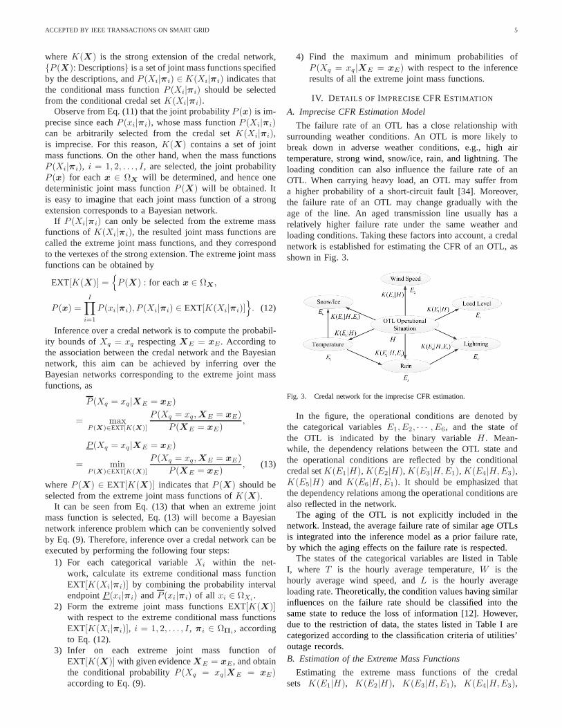
The failure rate of an OTL has a close relationship withsurrounding weather conditions. An OTL is more likely tobreak down in adverse weather conditions, e.g.,high airtemperature, strong wind, snow/ice, rain, and lightning. Theloading condition can also influence the failure rate of anOTL. When carrying heavy load, an OTL may suffer froma higher probability of a short-circuit fault [34]. Moreover,the failure rate of an OTL may change gradually with theage of the line. An aged transmission line usually has arelatively higher failure rate under the same weather andloading conditions. Taking these factors into account, a credalnetwork is established for estimating the CFR of an OTL, asshown in Fig. 3.

Fig. 3. Credal network for the imprecise CFR estimation.

In the figure, the operational conditions are denoted bythe categorical variablesE1, E2, · · · , E6, and the state ofthe OTL is indicated by the binary variableH . Mean-while, the dependency relations between the OTL state andthe operational conditions are reflected by the conditionalcredal setK(E1|H), K(E2|H), K(E3|H,E1), K(E4|H,E3),K(E5|H) and K(E6|H,E1). It should be emphasized thatthe dependency relations among the operational conditionsarealso reflected in the network.

The aging of the OTL is not explicitly included in thenetwork. Instead, the average failure rate of similar age OTLsis integrated into the inference model as a prior failure rate,by which the aging effects on the failure rate is respected.

The states of the categorical variables are listed in TableI, where T is the hourly average temperature,W is thehourly average wind speed, andL is the hourly averageloading rate.Theoretically, the condition values having similarinfluences on the failure rate should be classified into thesame state to reduce the loss of information [12]. However,due to the restriction of data, the states listed in Table I arecategorized according to the classification criteria of utilities’outage records.B. Estimation of the Extreme Mass Functions

Estimating the extreme mass functions of the credalsets K(E1|H), K(E2|H), K(E3|H,E1), K(E4|H,E3),

ACCEPTED BY IEEE TRANSACTIONS ON SMART GRID 6

TABLE ISTATES OF THECATEGORICAL VARIABLES

Variables State 1 State 2 State 3

E1

T ≤4°C(e1,1)

4°C< T ≤26°C(e1,2)

T >26°C(e1,3)

E2

W ≤12km/h(e2,1)

12km/h< W ≤40km/h(e2,2)

T >40km/h(e2,3)

E3

Rain(e3,1)

No Rain(e3,2)

N/A

E4

Lightning(e4,1)

No Lightning(e4,2)

N/A

E5

L ≤ 80%

(e5,1)L > 80%

(e5,2)N/A

E6

Snow/Ice(e6,1)

No Snow/Ice(e6,2)

N/A

HNormal Operation

(h1)Failure(h2)

N/A

K(E5|H) and K(E6|H,E1) is the first step for the CFRinference. To achieve this purpose, the endpoints of the con-ditional probabilities corresponding toP (E1|H), P (E2|H),P (E3|H,E1), P (E4|H,E3), P (E5|H) and P (E6|H,E1)have to be calculated using IDM, as expressed in Eq. (8).

For instance, to estimate the extreme mass functions ofthe conditional credal setK(E5|h2), which describes theuncertainty of the loading condition when the transmissionlinefails, the endpoints of the probability intervals correspondingto P (e5,1|h2) andP (e5,2|h2) have to be calculated, as

P (e5,1|h2) =nNL

nF + s, P (e5,1|h2) =

nNL + s

nF + s,

P (e5,2|h2) =nHL

nF + s, P (e5,2|h2) =

nHL + s

nF + s,

wherenNL andnHL are the numbers of samples for whichthe OTL breaks down with a normal and high loading rate,respectively, andnF = nNL +nHL is the number of samplesfor which the OTL breaks down in the relevant time interval.

Then the conditional credal setK(E5|h2) can be obtainedfrom Eq. (10) as

K(E5|h2) = CHP (E5|h2) :

P (e5,1|h2) ∈ [P (e5,1|h2), P (e5,1|h2)],

P (e5,2|h2) ∈ [P (e5,2|h2), P (e5,2|h2)],

P (e5,1|h2) + P (e5,2|h2) = 1.

Also, the extreme mass functions of the credal set canbe obtained by combining the endpoints of the probabilityintervals as

EXT[K(E5|h2)] =P (e5,1|h2) = P (e5,1|h2), P (e5,2|h2) = P (e5,2|h2)

andP (e5,1|h2) = P (e5,1|h2), P (e5,2|h2) = P (e5,2|h2)

.

Other conditional credal sets and corresponding extrememass functions can be calculated in the same way.

C. Imprecise CFR Inference with the Credal Network

With respect to the credal network mentioned above, thebounds of the CFR under specified operational conditions canbe calculated by the equations deduced from Eqs. (9), (12)and (13), as

λ = P (h2|e) = max

∏6j=1 P2,j · P (h2)

∑2i=1

∏6j=1 Pi,j · P (hi)

,

λ = P (h2|e) = min

∏6j=1 P2,j · P (h2)

∑2i=1

∏6j=1 Pi,j · P (hi)

,

when j = 1, 2, 5,

P2,j = P (ej,kj|h2), Pi,j = P (ej,kj

|hi),

when j = 3,

P2,j = P (e3,k3|h2, e1,k1

), Pi,j = P (e3,k3|hi, e1,k1

),

when j = 4,

P2,j = P (e4,k4|h2, e3,k3

), Pi,j = P (e4,k4|hi, e3,k3

),

when j = 6,

P2,j = P (e6,k6|h2, e1,k1

), Pi,j = P (e6,k6|hi, e1,k1

), (14)

where i is the index of OTL’s states,j is the index of theevidence variables,kj is used to specify the state of thejthevidence variable,P (h2) is the prior probability ofh2 whichis assigned by using the average failure rate of the OTLswithin the same age group,P (h1) = 1 − P (h2), P (ej,kj

|hi)is the conditional probability of the observationej,kj

givenhi with respect to the conditional mass functionP (Ej |hi),P (e3,k3

|hi, e1,k1) is the conditional probability ofe3,k3

givenhi ande1,k1

with respect toP (E3|hi, e1,k1), P (e4,k4

|hi, e3,k3)

is the conditional probability ofe4,k4given hi and e3,k3

with respect toP (E4|hi, e3,k3), and P (e6,k6

|hi, e1,k1) is

the conditional probability ofe6,k6given hi and e1,k1

with respect toP (E6|hi, e1,k1). Meanwhile, the conditional

mass functionP (Ej |hi), P (E3|hi, e1,k1), P (E4|hi, e3,k3

) andP (E6|hi, e1,k1

) are selected from the extreme mass functionsof the credal setK(Ej |hi), K(E3|hi, e1,k1

), K(E4|hi, e3,k3)

andK(E6|hi, e1,k1) to optimize the objective functions.

In (14), P (ej,kj|h2) is the occurrence probability of the

conditionej,kjgiven an OTL failure is observed. Considering

the deficiency of the failure samples, the probability shouldbe estimated using IDM. On the other hand,P (ej,kj

|h1) isthe occurrence probability of the condition given no OTLfailure happens. In this case, abundant samples are avail-able since no failure is a large probability event. And thisprobability can be approximated using the average occurrenceprobability of the condition to simplify the calculation, e.g.,P (e1,3|h1) ≈ P (e1,3) can be approximated by the statisticalprobability of high temperature in the relevant region. Theconditional probabilityP (e3,k3|hi, e1,k1), P (e4,k4|hi, e3,k3)andP (e6,k6|hi, e1,k1) can be obtained in the same way. Sincethe precise probability is a special case of the impreciseprobability, the CFR can still be estimated by using Eq. (14)under this circumstance.

V. CASE STUDIES

The proposed approach is tested by estimating the CFRs oftwo LGJ-300 transmission lines located in the same region.

ACCEPTED BY IEEE TRANSACTIONS ON SMART GRID 7

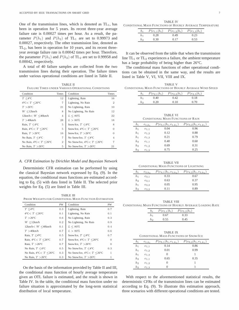
One of the transmission lines, which is denoted as TL1, hasbeen in operation for 5 years. Its recent three-year averagefailure rate is 0.00027 times per hour. As a result, the pa-rameterP (h1) and P (h2) of TL1 are set to 0.99973 and0.00027, respectively. The other transmission line, denoted asTL2, has been in operation for 10 years, and its recent three-year average failure rate is 0.00042 times per hour. Therefore,the parameterP (h1) andP (h2) of TL2 are set to 0.99958 and0.00042, respectively.

A total of 40 failure samples are collected from the twotransmission lines during their operation. The failure timesunder various operational conditions are listed in Table II.

TABLE IIFAILURE T IMES UNDER VARIOUS OPERATIONAL CONDITIONS

Condition Times Condition Times

T ≤4°C 12 Lightning, Rain 16

4°C< T ≤26°C 7 Lightning, No Rain 2

T >26°C 21 No Lightning, Rain 10

W ≤12km/h 8 No Lightning, No Rain 12

12km/h< W ≤40km/h 4 L ≤ 80% 22

T >40km/h 28 L > 80% 18

Rain,T ≤4°C 5 Snow/Ice,T ≤4°C 8

Rain, 4°C< T ≤26°C 5 Snow/Ice, 4°C< T ≤26°C 0

Rain,T >26°C 16 Snow/Ice,T >26°C 0

No Rain,T ≤4°C 7 No Snow/Ice,T ≤4°C 4

No Rain, 4°C< T ≤26°C 2 No Snow/Ice, 4°C< T ≤26°C 7

No Rain,T >26°C 5 No Snow/Ice,T >26°C 21

A. CFR Estimation by Dirichlet Model and Bayesian Network

Deterministic CFR estimation can be performed by usingthe classical Bayesian network expressed by Eq. (9). In theequation, the conditional mass functions are estimated accord-ing to Eq. (5) with data listed in Table II. The selected priorweights for Eq. (5) are listed in Table III.

TABLE IIIPRIOR WEIGHTS FORCONDITIONAL MASS FUNCTION ESTIMATION

Condition PW Condition PW

T ≤4°C 0.3 Lightning, Rain 0.7

4°C< T ≤26°C 0.1 Lightning, No Rain 0.1

T >26°C 0.6 No Lightning, Rain 0.3

W ≤12km/h 0.2 No Lightning, No Rain 0.9

12km/h< W ≤40km/h 0.1 L ≤ 80% 0.4

T >40km/h 0.7 L > 80% 0.6

Rain,T ≤4°C 0.5 Snow/Ice,T ≤4°C 0.7

Rain, 4°C< T ≤26°C 0.7 Snow/Ice, 4°C< T ≤26°C 0

Rain,T >26°C 0.7 Snow/Ice,T >26°C 0

No Rain,T ≤4°C 0.5 No Snow/Ice,T ≤4°C 0.3

No Rain, 4°C< T ≤26°C 0.3 No Snow/Ice, 4°C< T ≤26°C 1

No Rain,T >26°C 0.3 No Snow/Ice,T >26°C 1

On the basis of the information provided by Table II and III,the conditional mass function of hourly average temperaturegiven an OTL failure is estimated, and the result is shown inTable IV. In the table, the conditional mass function under nofailure situation is approximated by the long-term statisticaldistribution of local temperature.

TABLE IVCONDITIONAL MASS FUNCTIONS OFHOURLY AVERAGE TEMPERATURE

hi P (e1,1|hi) P (e1,2|hi) P (e1,3|hi)

h1 0.28 0.49 0.23h2 0.30 0.17 0.53

It can be observed from the table that when the transmissionline TL1 or TL2 experiences a failure, the ambient temperaturehas a large probability of being higher than 26°C.

The conditional mass functions of other operational condi-tions can be obtained in the same way, and the results arelisted in Table V, VI, VII, VIII and IX.

TABLE VCONDITIONAL MASS FUNCTIONS OFHOURLY AVERAGE WIND SPEED

hi P (e2,1|hi) P (e2,2|hi) P (e2,3|hi)

h1 0.40 0.42 0.18h2 0.20 0.10 0.70

TABLE VICONDITIONAL MASS FUNCTIONS OFRAIN

hi e1,k1P (e3,1|hi, e1,k1

) P (e3,2|hi, e1,k1)

h1 e1,1 0.04 0.96h1 e1,2 0.12 0.88h1 e1,3 0.21 0.79h2 e1,1 0.40 0.60h2 e1,2 0.69 0.31h2 e1,3 0.75 0.25

TABLE VIICONDITIONAL MASS FUNCTIONS OFL IGHTNING

hi e3,k3P (e4,1|hi, e3,k3

) P (e4,2|hi, e3,k3)

h1 e3,1 0.33 0.67h2 e3,1 0.63 0.37h1 e3,2 0.05 0.95h2 e3,2 0.11 0.89

TABLE VIIICONDITIONAL MASS FUNCTIONS OFHOURLY AVERAGE LOADING RATE

hi P (e5,1|hi) P (e5,2|hi)

h1 0.67 0.33h2 0.55 0.45

TABLE IXCONDITIONAL MASS FUNCTIONS OFSNOW/ICE

hi e1,k1P (e6,1|hi, e1,k1

) P (e6,2|hi, e1,k1)

h1 e1,1 0.14 0.86h1 e1,2 0.01 0.99h1 e1,3 0 1h2 e1,1 0.65 0.35h2 e1,2 0 1h2 e1,3 0 1

With respect to the aforementioned statistical results, thedeterministic CFRs of the transmission lines can be estimatedaccording to Eq. (9). To illustrate this estimation approach,three scenarios with different operational conditions aretested.

ACCEPTED BY IEEE TRANSACTIONS ON SMART GRID 8

Scenario I: The transmission line TL1 is operating normallynow. Its average loading rate will be 95% in the next hour. Atthe same time, according to the short-term weather forecast,a thunderstorm will come in the next hour. During the storm,the average air temperature will be 30°C and the wind speedwill be 48 km/h. Find the CFR of TL1 for the coming hour.

Scenario II: The transmission line TL1 is operating nor-mally now. In the next hour the temperature will be 15°C,the wind speed will be 10 km/h and the loading rate of thetransmission line will be less than 45%. Find the CFR of TL1

for the coming hour.Scenario III: The transmission line TL2 is operating nor-

mally now. All the operational conditions are the same asScenario I. Estimate the CFR of TL2 under this scenario.

The CFRs estimated by the Bayesian network are shown inTable X. It can be observed from the estimation results that theCFR of TL1 under Scenario I is much higher than that underScenario II. This is because all the operational conditionsofScenario I are adverse to power transmission compared withthat of Scenario II. On the other hand, it can be found fromthe results of Scenario I and Scenario III that the CFR of TL2

is obviously higher than that of TL1 under the same weatherand loading conditions. TL2 has a higher CFR because it ismuch older than TL1.

TABLE XESTIMATION RESULTS OF THEBAYESIAN NETWORK

Scenario I Scenario II Scenario III

2.19E−2 1.16E−5 3.37E−2

The estimation results of the deterministic approach maybe influenced by the prior weights dramatically. To illustratethis, a group of new prior weights are applied for the esti-mation, which are listed in Table XI. The corresponding CFRestimation results are shown in Table XII.

TABLE XIALTERNATIVE PRIOR WEIGHTS FOR THEMASS FUNCTION ESTIMATION

Condition PW Condition PW

T ≤4°C 0.4 Lightning, Rain 0.5

4°C< T ≤26°C 0.3 Lightning, No Rain 0.3

T >26°C 0.3 No Lightning, Rain 0.5

W ≤12km/h 0.2 No Lightning, No Rain 0.7

12km/h< W ≤40km/h 0.4 L ≤ 80% 0.8

T >40km/h 0.4 L > 80% 0.2

Rain,T ≤4°C 0.2 Snow/Ice,T ≤4°C 0.5

Rain, 4°C< T ≤26°C 0.5 Snow/Ice, 4°C< T ≤26°C 0

Rain,T >26°C 0.5 Snow/Ice,T >26°C 0

No Rain,T ≤4°C 0.8 No Snow/Ice,T ≤4°C 0.5

No Rain, 4°C< T ≤26°C 0.5 No Snow/Ice, 4°C< T ≤26°C 1

No Rain,T >26°C 0.5 No Snow/Ice,T >26°C 1

TABLE XIIESTIMATION RESULTS OF THEBAYESIAN NETWORK

Scenario I Scenario II Scenario III

2.05E−2 1.30E−5 3.15E−2

By comparing the estimation results shown in Table X andXII, it can be found that the estimated CFRs are differentwith different prior weights, which illustrates the significantinfluence of the prior weights on the CFR estimation results.

B. CFR Estimation by IDM and Credal Network

Using the historical observations shown in Table II, theimprecise conditional mass functions given OTL failures canbe obtained by using IDM according to Eq. (8), and the resultsare listed in Table XIII, XIV, XV, XVI, XVII and XVIII.

TABLE XIIIIMPRECISECONDITIONAL MASS FUNCTION OF TEMPERATURE

hi P (e1,1|hi) P (e1,2|hi) P (e1,3|hi)

h2 [0.29, 0.32] [0.17, 0.20] [0.51, 0.54]

TABLE XIVIMPRECISECONDITIONAL MASS FUNCTION OF WIND SPEED

hi P (e2,1|hi) P (e2,2|hi) P (e2,3|hi)

h2 [0.19, 0.22] [0.10, 0.13] [0.68, 0.71]

TABLE XVIMPRECISECONDITIONAL MASS FUNCTION OF RAIN

hi e1,k1P (e3,1|hi, e1,k1

) P (e3,2|hi, e1,k1)

h2 e1,1 [0.38, 0.46] [0.54, 0.62]h2 e1,2 [0.63, 0.75] [0.25, 0.37]h2 e1,3 [0.73, 0.77] [0.23, 0.27]

TABLE XVIIMPRECISECONDITIONAL MASS FUNCTION OF L IGHTNING

hi e3,k3P (e4,1|hi, e3,k3

) P (e4,2|hi, e3,k3)

h2 e3,1 [0.59, 0.63] [0.37, 0.41]h2 e3,2 [0.08, 0.15] [0.85, 0.92]

TABLE XVIIIMPRECISECONDITIONAL MASS FUNCTION OF HOURLY AVERAGE

LOADING RATE

hi P (e5,1|hi) P (e5,2|hi)

h1 [0.54, 0.56] [0.44, 0.46]

TABLE XVIIIIMPRECISECONDITIONAL MASS FUNCTION OF SNOW/ICE

hi e6,k1P (e6,1|hi, e1,k1

) P (e6,2|hi, e1,k1)

h2 e1,1 [0.62, 0.69] [0.31, 0.38]h2 e1,2 [0, 0.12] [0.88, 1]h2 e1,3 [0, 0.04] [0.96, 1]

It is observed from the tables that the conditional proba-bilities estimated by the deterministic Dirichlet model are allincluded in the probability intervals estimated by the IDM,which illustrates the rationality of the IDM estimation results.The widths of the probability intervals estimated by the IDMquantitatively reflect the uncertainty existed in the probabilityestimation results.

Respecting the estimation results of IDM, the impreciseCFRs corresponding to the three scenarios can be calculatedaccording to Eq. (14), and the results are listed in Table XIX.

It can be found that the estimation results of the Bayesiannetwork with different prior weights are all included in theprobability intervals estimated by the credal network. In fact,this phenomenon is universal, which verifies that the proposed

ACCEPTED BY IEEE TRANSACTIONS ON SMART GRID 9

TABLE XIXESTIMATION RESULTS OF THECREDAL NETWORK

Scenario I Scenario II Scenario III

[1.85E−2, 2.38E−2] [8.88E−6, 1.94E−5] [2.85E−2, 3.66E−2]

approach can eliminate the subjectivity caused by the priorweight assignment. Furthermore, it can be found by comparingthe estimation results corresponding to different scenarios thatthe effects of the weather, loading and aging conditions onthe CFRs can also be reflected in the estimation results of thecredal network.

Sometimes, the occurrence of the operational conditions isuncertain. For instance, it is difficult to exactly predict the airtemperature in the coming hour. The proposed approach canhandle such uncertainty conveniently by using the law of totalprobability, as illustrated by the following example.

Scenario IV: The transmission line TL2 is operating nor-mally now. All the operational conditions are the same as inScenario I except that the wind speed has a 70% probabilityof being faster than 40 km/h and a 30% probability of rangingfrom 12 km/h to 40 km/h.

Under this scenario, the CFR is estimated to be within[2.05 × 10−2, 2.65 × 10−2]. Comparing this result with theimprecise CFR estimation result of Scenario III, it can befound that the CFR is lower under Scenario IV. This is becausethe wind speed has a considerable probability of being slowin Scenario IV, which is beneficial for the power transmission.

C. Comparison with Other Probability Interval EstimationApproaches

A simulation system is set up to compare the performanceof the proposed approach and two existing approaches, i.e.,thecentral limit theorem based approach [12] and the Chi-squaredistribution based approach [13]. To simplify the analysis, theoperational conditions are categorized into two groups, i.e.,the normal operational condition and the adverse operationalcondition, and the occurrence probabilities of these two op-erational conditions are 0.7 and 0.3, respectively. Assumethefailure rates of the interested OTL under normal and adverseoperational conditions are 0.0001 and 0.005, respectively. Thesimulation system is virtually operated for 10000 hours, andthe collected failure and operational condition data are usedto estimate the CFR of the OTL.

The CFR interval under the adverse operational conditionis estimated by using the aforementioned approaches, and theresults are shown in Fig. 4.

From the figure, the following facts can be observed.

1) The CFR intervals estimated by all the approaches canconverge to the real CFR as data accumulate. Mean-while, the interval of the proposed approach convergesmuch faster than those of the existing approaches.

2) When the sample size is small, the CFR interval esti-mated by the Chi-square distribution based approach isvery large. The upper bound of the estimated intervalis even greater than 1, mainly because the equivalentChi-square distribution is unbounded on the right side.

Fig. 4. CFR intervals under the adverse operational condition.

3) The central limit theorem based approach cannot per-form the interval estimation until the occurrence of thefirst failure. Meanwhile, the lower bound of the esti-mated interval may be less than 0 because the convertednormal distribution is unbounded.

The observations illustrate that the proposed approach canobtain more reasonable and more accurate CFR intervals thanthe existing approaches.

VI. CONCLUSION

Because of the deficiency of the OTL failure samples, theCFR estimation result may be unreliable in practice. Underthis circumstance, a novel imprecise probabilistic approach forthe CFR estimation, based on IDM and the credal network,is proposed. In the approach, IDM is adopted to estimatethe imprecise probabilistic dependency relations betweentheOTL failure and the operational conditions, and the credalnetwork is established to integrate the IDM estimation resultsand infer the imprecise CFR. The proposed approach is testedby estimating the CFRs of two transmission lines located inthe same region. The test results illustrate that: a) the proposedapproach can quantitatively evaluate the uncertainty of the es-timated CFR by using the interval probability, b) the influencesof the operational conditions on the CFR can be properlyreflected in the estimation result, and c) the uncertainty ofthe operational conditions can also be handled by using theproposed approach.Moreover, a simulation system is set upto demonstrate the advantages of the proposed approach overthe existing approaches, i.e., the central limit theorem basedapproach and the Chi-square distribution based approach. Thetest results indicate that the CFR interval estimated by theproposed approach is much tighter and more reasonable thanthose obtained by the existing approaches.

ACCEPTED BY IEEE TRANSACTIONS ON SMART GRID 10

APPENDIX ATHE CREDIBLE INTERVAL

The credible intervalD = [a, b] is the interval that ensuresthe posterior lower probability PrPm ∈ D reaches a speci-fied credibilityγ, e.g.,γ = 0.95, wherePm is the probabilitycorresponding to themth outcome of the multinomial variable.

The bounds ofD can be obtained by

a = 0, b = G−1(1+γ2

), nm = 0,

a = H−1(1−γ2

), b = G−1

(1+γ2

), 0 < nm < n,

a = H−1(1−γ2

), b = 1, nm = n,

(15)

where H is the cumulative distribution function (CDF) ofbeta distributionB(nm, s + n − nm), G is the CDF of betadistributionB(s + nm, n− nm), n is the sample size,nm isthe number of times that themth outcome is observed, andsis the equivalent sample size that is set to 1 [27].

APPENDIX BCOMPARISON OF THEPROBABILITY INTERVAL COUNTING

APPROACHES

Probability intervals counted from available samples are thebasis of the proposed approach. The performance of severalcounting approaches, i.e., IDM, the credible interval estimationapproach, the central limit theorem based approach [12], andthe Chi-square distribution based approach [13], is tested.The samples are randomly selected from Poisson distributionPois(0.01), which means for each sample the correspondingtwo-state random variable has a 1% chance to be 1 and a 99%chance to be 0. The test results are shown in Fig. 5.

Fig. 5. Probability intervals estimated by different methods.

From the results, the following facts can be observed.

1) IDM can obtain the tightest probability interval that alsoconverges much faster than the other approaches. Mean-while, when the sample size is smaller than 25, the 95%credible interval obtained by the approach in AppendixA is obviously tighter than the 95% confidence intervalestimated by the Chi-square distribution based approach.

2) The upper bound of the probability interval estimatedby the Chi-square distribution based approach may begreater than 1 (see the confidence intervals correspond-ing to the first three samples), which is obviouslyunreasonable.

3) The central limit theorem based approach cannot obtaina meaningful probability interval until all the states ofthe two-state variable occur at least once. Moreover, theestimated lower bound may be less than 0 because theconverted normal distribution is unbounded.

The observations illustrate that IDM and the correspondingcredible interval estimation approach can provide more reason-able estimation results compared with the existing approaches.

In this paper, IDM is used to estimate the uncertain proba-bilistic dependency relations between the OTL failure and theoperational conditions. Meanwhile, the credible intervalesti-mation approach mentioned in Appendix A is recommendedas an alternative if a quantitative confidence index is required.

APPENDIX CEFFECTS OF THEEQUIVALENT SAMPLE SIZE

The equivalent sample sizes can influence the estimation re-sult of IDM. In fact,s determines how quickly the probabilityinterval will converge as data accumulate. Smaller values of sproduce faster convergence and stronger conclusions, whereaslarger values ofs produce more cautious inferences. Morespecifically, s indicates the number of observations neededto reduce the length of the imprecision interval to half of itsinitial value (according to Eq. (8), the length of the imprecisioninterval is∆Pm = Pm−Pm = s/(n+s), which will decreasefrom 1 to 1/2 whenn increases from0 to s).

Therefore, the assignment ofs reflects the cautiousnessof the estimation. To obtain objective estimation results,assuggested by Walley in [27], the value ofs should be suffi-cient large to encompass all reasonable probability intervalsestimated by various objective Bayesian alternatives. Up tonow, several researches have led to convincing arguments thats should be chosen from[1, 2], and the value ofs shouldbe larger when the multinomial variable has a large numberof states [25]. In our model, since the multinomial variablesonly have 2 or 3 states (see Table I), the parameters is setto 1 as suggested. Moreover, it should be emphasized thatthe influence ofs weakens quickly as the number of samplesincreases, which can be clearly seen from Fig. 6. It can also beobserved from the figure that all of the probability intervalsestimated by IDM (1 ≤ s ≤ 2) converge faster than thatestimated by the Chi-square distribution based approach.

REFERENCES

[1] R. Allan et al., Reliability evaluation of power systems. SpringerScience & Business Media, 2013.

[2] R. Billinton and P. Wang, “Teaching distribution systemreliabilityevaluation using Monte Carlo simulation,”IEEE Trans. Power Syst.,vol. 14, no. 2, pp. 397–403, Aug. 1999.

[3] J. Qi, S. Mei, and F. Liu, “Blackout model considering slow process,”IEEE Trans. Power Syst., vol. 28, no. 3, pp. 3274–3282, Aug. 2013.

[4] D. Koval and A. Chowdhury, “Assessment of transmission-line common-mode, station-originated, and fault-type forced-outage rates,” IEEETrans. Ind. Appl., vol. 46, no. 1, pp. 313–318, Jan. 2010.

ACCEPTED BY IEEE TRANSACTIONS ON SMART GRID 11

Fig. 6. Probability intervals estimated with different equivalent sample sizes.

[5] J. Qi, K. Sun, and S. Mei, “An interaction model for simulation andmitigation of cascading failures,”IEEE Trans. Power Syst., vol. 30, no. 2,pp. 804–819, Jul. 2015.

[6] J. Qi, W. Ju, and K. Sun, “Estimating the propagation of interdependentcascading outages with multi-type branching processes,”IEEE Trans.Power Syst., to be published.

[7] C. Williams, “Weather normalization of power system reliability in-dices,” in IEEE Power Eng. Soc. General Meeting. Tampa, FL, USA,Sep. 7-12, 2007, pp. 1–5.

[8] L. Ning, W. Wu, B. Zhang, and P. Zhang, “A time-varying transformeroutage model for on-line operational risk assessment,”Int. J. Elec.Power, vol. 33, no. 3, pp. 600–607, Mar. 2011.

[9] Y. Feng, W. Wu, B. Zhang, and W. Li, “Power system operation riskassessment using credibility theory,”IEEE Trans. Power Syst., vol. 23,no. 3, pp. 1309–1318, Aug. 2008.

[10] R. Billinton and G. Singh, “Application of adverse and extreme adverseweather: modelling in transmission and distribution system reliabilityevaluation,” Proc. Inst. Elect. Eng., Gen., Transm. Distrib., vol. 153,no. 1, pp. 115–120, Jan. 2006.

[11] R. Billinton and W. Li, “A novel method for incorporating weathereffects in composite system adequacy evaluation,”IEEE Trans. PowerSyst., vol. 6, no. 3, pp. 1154–1160, Aug. 1991.

[12] Y. Zhou, A. Pahwa, and S. S. Yang, “Modeling weather-related failuresof overhead distribution lines,”IEEE Trans. Power Syst., vol. 21, no. 4,pp. 1683–1690, Nov. 2006.

[13] W. Li, J. Zhou, and X. Xiong, “Fuzzy models of overhead power lineweather-related outages,”IEEE Trans. Power Syst., vol. 3, no. 23, pp.1529–1531, Aug. 2008.

[14] H. L. Willis, “Panel session on: aging t&d infrastructures and customerservice reliability,” in IEEE Power Eng. Soc. Summer Meeting, vol. 3.Seattle, WA, USA, Jul. 16-20, 2000, pp. 1494–1496.

[15] P. Carer and C. Briend, “Weather impact on components reliability: Amodel for mv electrical networks,” inProc. the 10th Int. Conf. PMAPS,.Rincon, Puerto Rico, USA, May 25-29, 2008, pp. 1–7.

[16] M. Bollen, “Effects of adverse weather and aging on power systemreliability,” IEEE Trans. Ind. Appl., vol. 37, no. 2, pp. 452–457, Mar.2001.

[17] Y. Ding, M. J. Zuo, A. Lisnianski, and Z. Tian, “Fuzzy multi-statesystems: general definitions, and performance assessment,” IEEE Trans.Reliab., vol. 57, no. 4, pp. 589–594, Dec. 2008.

[18] Y. Ding and A. Lisnianski, “Fuzzy universal generatingfunctions formulti-state system reliability assessment,”Fuzzy Set. Syst., vol. 159,no. 3, pp. 307–324, Feb. 2008.

[19] R. E. Walpole, R. H. Myers, S. L. Myers, and K. Ye,Probability andstatistics for engineers and scientists. Macmillan New York, 1993,vol. 5.

[20] N. L. Johnson, A. W. Kemp, and S. Kotz,Univariate discrete distribu-tions. John Wiley & Sons, 2005, vol. 444.

[21] P. Walley,Statistical Reasoning with Imprecise Probabilities. Chapman& Hall, 1991.

[22] F. Coolen, “An imprecise Dirichlet model for Bayesian analysis of failuredata including right-censored observations,”Reliab. Eng. Syst. Safe.,vol. 56, no. 1, pp. 61–68, Apr. 1997.

[23] C. Li, X. Chen, X. Yi, and J. Tao, “Interval-valued reliability analysis ofmulti-state systems,”IEEE Trans. Reliab., vol. 60, no. 1, pp. 323–330,Mar. 2011.

[24] M. Finkelstein, Failure Rate Modelling for Reliability and Risk.Springer, 2008.

[25] J. M. Bernard, “An introduction to the imprecise Dirichlet model formultinomial data,”Int. J. Approx. Reason., vol. 39, no. 2, pp. 123–150,Jun. 2005.

[26] A. R. Masegosa and S. Moral, “Imprecise probability models forlearning multinomial distributions from data. Applications to learningcredal networks,”Int. J. Approx. Reason., vol. 55, no. 7, pp. 1548–1569,Oct. 2014.

[27] P. Walley, “Inferences from multinomial data: learning about a bag ofmarbles,”J. R. Stat. Soc. B, vol. 58, no. 1, pp. 3–57, Jan. 1996.

[28] A. Antonucci, A. Piatti, and M. Zaffalon, “Credal networks for op-erational risk measurement and management,” inKnowledge-BasedIntelligent Information and Engineering Systems. Springer, 2007, pp.604–611.

[29] D. Heckerman, A Tutorial on Learning with Bayesian Networks.Springer, 1998.

[30] F. G. Cozman, “Credal networks,”Artif. Intell., vol. 120, no. 2, pp.199–233, Jul. 2000.

[31] F. G. Cozman, “Graphical models for imprecise probabilities,” Int. J.Approx. Reason., vol. 39, no. 2, pp. 167–184, Jun. 2005.

[32] J. Abellan and M. Gomez, “Measures of divergence on credal sets,”Fuzzy Set. Syst., vol. 157, no. 11, pp. 1514–1531, Jun. 2006.

[33] G. Corani, A. Antonucci, and M. Zaffalon, “Bayesian networks withimprecise probabilities: Theory and application to classification,” in DataMining: Foundations and Intelligent Paradigms. Springer, 2012, pp.49–93.

[34] W. Christiaanse, “Reliability calculations including the effects of over-loads and maintenance,”IEEE Trans. Power Appa. & Syst., no. 4, pp.1664–1677, Jul. 1971.