IOP PUBLISHING JOURNAL OF PHYSICS D: APPLIED PHYSICS
J. Phys. D: Appl. Phys. 46 (2013) 025301 (9pp) doi:10.1088/0022-3727/46/2/025301
Achieving concentrated graphenedispersions in water/acetone mixturesby the strategy of tailoring Hansensolubility parametersMin Yi, Zhigang Shen, Xiaojing Zhang and Shulin Ma
Beijing Key Laboratory for Powder Technology Research & Development, Beijing University ofAeronautics and Astronautics, Beijing 100191, People’s Republic of China
Received 10 July 2012, in final form 13 July 2012Published 5 December 2012Online at stacks.iop.org/JPhysD/46/025301
AbstractAlthough exfoliating graphite to give graphene paves a new way for graphene preparation, ageneral strategy of low-boiling-point solvents and high graphene concentration is still highlyrequired. In this study, using the strategy of tailoring Hansen solubility parameters (HSP), amethod based on exfoliation of graphite in water/acetone mixtures is demonstrated to achieveconcentrated graphene dispersions. It is found that in the scope of blending two mediocresolvents, tailoring the HSP of water/acetone mixtures to approach the HSP of graphene couldyield graphene dispersions at a high concentration of up to 0.21 mg ml−1. The experimentallydetermined optimum composition of the mixtures occurs at an acetone mass fraction of ∼75%.The trend of concentration varying with mixture compositions could be well predicated by themodel, which relates the concentration to the mixing enthalpy within the scope of HSP theory.The resultant dispersion is highly stabilized. Atomic force microscopic statistical analysisshows that up to ∼50% of the prepared nanosheets are less than 1 nm thick after 4 h sonicationand 114g centrifugation. Analyses based on diverse characterizations indicate the graphenesheets to be largely free of basal plane defects and oxidation. The filtered films are alsoinvestigated in terms of their electrical and optical properties to show reasonable conductivityand transparency. The strategy of tailoring HSP, which can be easily extended to varioussolvent systems, and water/acetone mixtures here, extends the scope for large-scale productionof graphene in low-boiling-point solutions.
(Some figures may appear in colour only in the online journal)
1. Introduction
Graphene, a two-dimensional material, has attractedconsiderable attention for a broad range of potentialapplications due to its excellent properties [1–5]. As thefirst step to investigate its properties and eventually to takeit to real-world applications, graphene should be prepared inlarge quantities for large-scale applications. Various methodshave been proposed to prepare graphene [6–40]. And recentdevelopments in liquid-phase exfoliation of graphite to givegraphene [6, 7, 12, 15, 17–22, 24, 25, 28–38] signify that it ispossible to easily prepare low-cost graphene on a large scale
for applications in electrodes, transparent films, compositeformulation, surface patterning, etc.
However, there are still some problems. The liquid-phase medium used in the exfoliation process mainly includesorganic solvents [19, 24, 25, 30, 35, 38], ionic liquid [17,34], and water with surfactants or polymers as stabilizers[6, 7, 12, 18, 20–22, 29, 33, 36, 37]. On the one hand, it isdifficult to remove residual surfactants [7, 12, 20, 22, 29, 33,36, 37] or polymers [6, 18, 21] when processing graphenefrom water with stabilizers. On the other hand, althoughorganic solvents such as N -methylpyrrolidone (NMP) canachieve high-quality graphene dispersions, they are not without
J. Phys. D: Appl. Phys. 46 (2013) 025301 M Yi et al
drawbacks. It has been pointed out that the best organicsolvents tend to be toxic and have high boiling points [25, 28,31, 41], making them difficult to handle during the preparationprocess and to remove when graphene films or composites areformed. Also, this makes it impossible to deposit individualflakes because of aggregation during the slow solventevaporation. In addition, in order to make many applicationspractical, a graphene dispersion with a concentration ofseveral hundred µg ml−1 is required. Although someup-to-date work has reported high-concentration graphenedispersions prepared in high boiling point solvents [19, 38]and surfactant-stabilized water [20], these processes stronglyrely on sonication for an extremely long time (several hundredhours), which may introduce additional defects and lower thethroughput. So it would be preferable to achieve concentratedgraphene dispersions in green and low-boiling-point solventsby sonication for a not very long time.
In this study, with the above-mentioned points in mind,based on the strategy of tailoring Hansen solubility parameters(HSP), we demonstrate a method to prepare concentratedgraphene dispersions in water/acetone mixtures by sonicationfor several hours. We also noted that, some researchersrecently found that graphite powders could form stabledispersion in the water/acetone mixtures [42], but they did notgo further to optimize processing to achieve graphene and didnot give a criterion to guide the process of producing grapheneby mixing solvents. Herein, we go further to achieve high-quality concentrated graphene dispersion in water/acetonemixtures and demonstrate a HSP strategy to guide this method.Compared to the previously published work about dispersinggraphite [42], the novelty of our work mainly lies in producinggraphene in green low-boiling-point solvents and proposing acriterion for designing solvent mixtures to produce graphene.In our work, water and acetone are previously thought aspoor solvents or nonsolvents for graphene due to their HSPmismatching those of graphene, but mixing water and acetonecan tailor the solubility parameters to obtain ideal solventsystems. The optimum mixing ratio could be roughly predictedby the HSP theory. And the trend of concentration varyingwith mixture compositions could be predicted well by themodel, which relates the concentration to the mixing enthalpywithin the scope of HSP theory. Diverse characterizationtechniques have been used to analyse the resultant grapheneand its dispersion. This method has vital advantages becausewater is a totally green solvent and acetone is a frequentlyused cheap solvent with a low boiling point of 58 ◦C. Becausethe number of solvent mixtures is limitless, the strategy oftailoring HSP allows researchers great freedom in designingideal solvent systems for specific applications.
2. Experimental
A graphite dispersion was prepared by adding graphite(particle sizes � 300 meshes) at an initial concentration of3 mg ml−1 to 30 ml water/acetone mixtures in a steel vesselwith inner diameter 30 mm. A graphene dispersion wasprepared by sonicating this graphite dispersion for differenttimes (2, 4, 6, 8, 12 h), followed by centrifugation at different
speeds, from 500 to 4000 rpm (36–2276g) for 30 min (XiangyiL600). Various mixing ratios of water and acetone in mixtureswere explored to find the optimum mixing ratio. For eachmixing ratio, at least five samples were repeated. The steelvessel was fixed at the same position in the sonic bath (KexiKX1620) during the whole experiment. Continuous refilling ofbath water was carried out to maintain the sonication efficiencyand prevent overheating. The true power output into the steelvessel was estimated to be 0.8 W by measuring the temperaturerise while sonicating a known mass of water. Grapheneconcentration after centrifugation and standing for one week,CG, was determined from A/l = αCG, where A/l wasmeasured at 660 nm by a 721E spectrophotometer (ShanghaiSpectrum) and the absorption coefficient α was determinedexperimentally based on Lambert–Beer behaviour. Filteredthin films with a diameter of 40 mm were prepared by vacuumfiltration onto porous mixed cellulose membranes (pore size:220 nm). These films were punched into several small circularpieces and then transferred onto glass slides with the filtermembrane dissolved by acetone. After drying at 80 ◦C forabout 120 min, the small thin films deposited on slide glasseswere used for optical and electrical measurements.
UV–vis spectra of the graphene dispersion were recordedon a Purkinje General TU1901 UV–vis spectrometer. Scanningelectron microscopy (SEM) images were collected by aLEO 1530VP. Atomic force microscope (AFM) images werecaptured with a CSPM5500 AFM (Being Nano-Instruments)in tapping mode. Bright-field transmission microscope (TEM)and high-resolution TEM (HRTEM) images were taken witha JEOL 2100 operating at 200 kV. Raman measurementswere made on these films with a Renishaw Rm2000 usinga 514 nm laser, where ten spectra were collected and theID/IG ratio was averaged. X-ray diffraction (XRD) patternsof the filtered film were collected using Cu Kα radiation (λ =1.5418 Å) with an x-ray diffractometer (Bruke D8-advance)operating at 40 kV and 40 mA. Fourier transformer infrared(FTIR) spectrum of the filtered film (collected as powder) wasmeasured by a Nicolet Nexus870 spectrometer using the KBrpellet technique. X-ray photoelectron spectroscopy (XPS)investigation was performed on the filtered film dried in airby an ESCALAB-250 photoelectron spectrometer (ThermoFisher Scientific). Optical transmission spectra of the filmsdeposited on glass slides were recorded on a Purkinje GeneralTU1901 UV–vis spectrometer with a glass slide as reference.Sheet resistance, Rs, was measured by a KDY-1 four-proberesistivity test system (GuangZhou KunDe).
3. Results and discussion
The absorption coefficient, α, which is related to theabsorbance per unit path length, A/l, through the Lambert–Beer law A/l = αC, is an important parameter incharacterizing any dispersion. In order to accurately ascertainthe graphene concentration, the absorption coefficient, α, mustbe determined experimentally. So we prepared a large volumeof graphene dispersion in water/acetone mixtures (75 wt%acetone, which was determined as follows, 4 h sonication,1000 rpm). Based on five graphene dispersion samples whose
2
zhk
铅笔
www.spm
.com
.cn
J. Phys. D: Appl. Phys. 46 (2013) 025301 M Yi et al
Figure 1. Absorbance per unit path length (λ = 660 nm), A/l, as afunction of concentration of graphene, CG, in water/acetonemixtures (75 wt% acetone). Lambert–Beer behaviour is shown, withan absorption coefficient α = 3600 ml mg−1 m−1. Inset: absorptionspectra for graphene dispersed in water/acetone mixtures (75 wt%acetone) at concentrations from 8.75 to 25.6 µg ml−1.
concentrations were determined by measuring the dispersionvolume and weighing the graphene film after filtration anddrying, we could obtain the accurate relationship betweengraphene concentration, CG, and absorbance per unit pathlength, A/l, as shown in figure 1. A straight line fit throughthese points gives an absorption coefficient at 660 nm of α =3600 ml mg−1 m−1, which agrees with the reported value inhigh-concentration graphene dispersions [19, 38]. It should benoted that the value of α remains nearly constant regardlessof the solvent composition [25]. Absorption spectra of thegraphene dispersion with different concentrations were alsomeasured (inset of figure 1). As expected for a quasi-two-dimensional material, the spectra are featureless in the visibleregion [43].
We optimized the mixing ratio of water and acetone bymeasuring the concentration (proportional to A/l) of grapheneremaining dispersed after sonication and centrifugation as afunction of acetone mass fraction (4 h sonication, 1000 rpm). Ithas been proved that the rotation rates of 25g was the minimumrequired to remove large aggregates, while the rotation ratesof more than 400g could result in graphene with considerablebody defects [20]. Thus, we chose an interval value, 1000 rpm(144g), to obtain a graphene dispersion. The results are shownin figure 2, where the graphene concentration highly dependson the acetone mass fraction. Appreciable discrepancies ofgraphene concentration under different mixing ratios are clearto the naked eye, as presented in figure 2(a). Pure water andpure acetone produce only an almost transparent dispersion,while at an appropriate acetone mass fraction a dark blackgraphene dispersion can be obtained. From figure 2(b), it canbe seen that the maximum graphene concentration occurs atan acetone mass fraction of ∼75%, which can be taken as theoptimum mixing ratio. The maximum graphene concentrationduring centrifugation of 1000 rpm reaches ∼0.11 mg ml−1,which is several hundred times higher than that in purewater or acetone. This maximum graphene concentration
Figure 2. (a) Photos of graphene dispersions in variouswater/acetone mixtures after 4 h sonication and 1000 rpmcentrifugation, which have been stored under ambient conditions fora week. (b) Graphene concentration, CG, and the calculated Ra and�G, as a function of the acetone mass fraction. CG, Ra and �G areshown as dots, a dotted line and a solid line, respectively.
of ∼0.11 mg ml−1, achieved in the water/acetone mixtures,is comparable to the previously reported maximum values inNMP [19] and sodium cholate stabilized water [20]. However,those reported high-concentration graphene dispersions wereachieved by sonication for several hundred hours [19, 20].
As for the theoretical considerations of optimizing themixing ratio, we turn to the HSP theory [44, 45]. It hasbeen evidenced that good solvents should have HSP matchingthose of graphene [28, 31, 41]. And blending two mediocresolvents, water and acetone, can tailor the solubility parametersof the mixtures to approach the HSP of graphene [44, 45].According to Hansen, each solvent or material has threeHansen parameters: δD, δP and δH, which can be located in the3D Hansen space just as co-ordinates [44, 45]. In the Hansenspace, between solvent 1 and solute 2, HSP distance Ra isdefined as Ra = (4(δD1−δD2)
2 +(δP1−δP2)2 +(δH1−δH2)
2)1/2.Hence the idea is the smaller the Ra, the higher the solubility[44, 45]. Additionally, the HSP of a mixture is proportional tothe volume fractions of its component solvents [44, 45]. So forthe water/acetone mixtures here, δi,mix = ((1 − φa)/ρwδi,w +φa/ρaδi,a)/((1 − φa)/ρw + φa/ρa), where i denotes D, P orH, φa denotes the acetone mass fraction, ρw and ρa denote thedensity of water and acetone, respectively. Based on the HSP ofgraphene [41], which has been estimated as δD,G ∼ 18 MPa1/2,δP,G ∼ 9.3 MPa1/2 and δH,G ∼ 7.7 MPa1/2, and the HSPof water [45] (δD ∼ 18.1 MPa1/2, δP ∼ 17.1 MPa1/2 andδH ∼ 16.9 MPa1/2, correlation with total miscibility) andacetone [45] (δD ∼ 15.5 MPa1/2, δP ∼ 10.4 MPa1/2 andδH ∼ 7 MPa1/2), Ra between graphene and the water/acetone
3
www.spm
.com
.cn
J. Phys. D: Appl. Phys. 46 (2013) 025301 M Yi et al
mixture can be calculated, as shown by the dotted line infigure 2(b). It can be seen that the smallest Ra occurs aroundthe highest concentration. However, it should be noted thatRa here has a very broad minimum in the 60–90% range. Inthis broad range, it is strange that such small changes in Rasurprisingly lead to such a sharp change in the solubility ofgraphene. This phenomenon cannot be explained perfectly inthe scope of Ra. Hence, we further try a more sophisticatedmodel within the HSP theory, relating mixing enthalpy tographene concentration. It has been proposed that, similar tothe case of nanotube, the dispersion concentration of graphene,�G, can be given by [28]
�G ∝ exp
[− v
RT
∂(H/V )
∂ϕ
],
where v is the molar volume of graphene which is a constant,H/V is the enthalpy of mixing per volume of the mixture(graphene and solvents), ϕ is the dispersed graphene volumefraction. According to Hansen [44, 45], the enthalpy of mixingcan be written as
H
V≈ ϕ(1 − ϕ)
[(δD,mix − δD,G)2 +
1
4(δP,mix − δP,G)2
+1
4(δH,mix − δH,G)2
].
Considering that the volume fraction of dispersed graphene isvery low (1 − ϕ ≈ 1) and v/RT remains constant, we canobtain that
Thus, we can plot the relationship between �G and acetonemass fraction, as shown by the solid line in figure 2(b).Obviously, in the scope of �G, the predicted trend ofconcentration varying with acetone mass fraction agreesbetter with the experimental data. So it can be concludedthat by tailoring the HSP of the water/acetone mixtures toapproach the HSP of graphene, mixing water and acetonecan yield concentrated graphene dispersions. And the trendof concentration varying with mixture compositions could bewell predicated by the model which relates the concentration tothe mixing enthalpy within the scope of HSP theory. Based onthe above discussion, we can deduce that the physical origin ofour results lies in that: mixing blending two mediocre solvents(for example, water and acetone used here) can tailor the HSPof mixed solvents to approach the HSP of graphene, thusminimizing the enthalpy of mixing and obtaining concentratedand stable graphene dispersion.
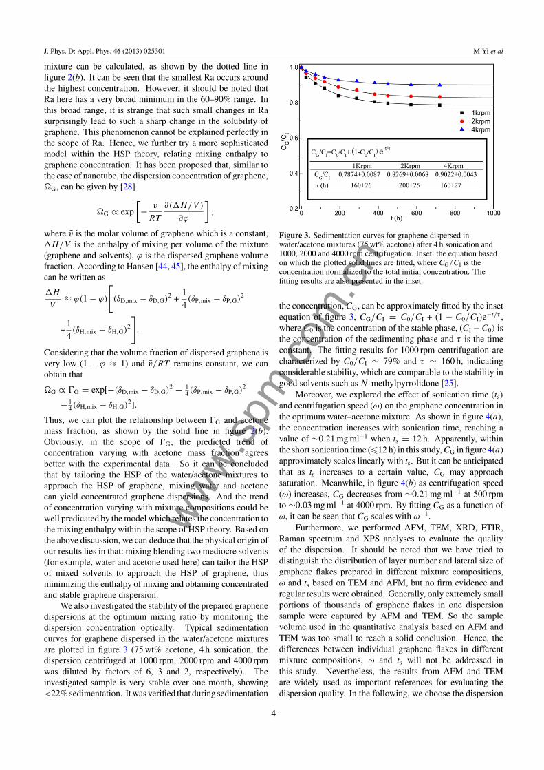
We also investigated the stability of the prepared graphenedispersions at the optimum mixing ratio by monitoring thedispersion concentration optically. Typical sedimentationcurves for graphene dispersed in the water/acetone mixturesare plotted in figure 3 (75 wt% acetone, 4 h sonication, thedispersion centrifuged at 1000 rpm, 2000 rpm and 4000 rpmwas diluted by factors of 6, 3 and 2, respectively). Theinvestigated sample is very stable over one month, showing<22% sedimentation. It was verified that during sedimentation
Figure 3. Sedimentation curves for graphene dispersed inwater/acetone mixtures (75 wt% acetone) after 4 h sonication and1000, 2000 and 4000 rpm centrifugation. Inset: the equation basedon which the plotted solid lines are fitted, where CG/CI is theconcentration normalized to the total initial concentration. Thefitting results are also presented in the inset.
the concentration, CG, can be approximately fitted by the insetequation of figure 3, CG/CI = C0/CI + (1 − C0/CI)e−t/τ ,where C0 is the concentration of the stable phase, (CI − C0) isthe concentration of the sedimenting phase and τ is the timeconstant. The fitting results for 1000 rpm centrifugation arecharacterized by C0/CI ∼ 79% and τ ∼ 160 h, indicatingconsiderable stability, which are comparable to the stability ingood solvents such as N -methylpyrrolidone [25].
Moreover, we explored the effect of sonication time (ts)and centrifugation speed (ω) on the graphene concentration inthe optimum water–acetone mixture. As shown in figure 4(a),the concentration increases with sonication time, reaching avalue of ∼0.21 mg ml−1 when ts = 12 h. Apparently, withinthe short sonication time (�12 h) in this study, CG in figure 4(a)approximately scales linearly with ts. But it can be anticipatedthat as ts increases to a certain value, CG may approachsaturation. Meanwhile, in figure 4(b) as centrifugation speed(ω) increases, CG decreases from ∼0.21 mg ml−1 at 500 rpmto ∼0.03 mg ml−1 at 4000 rpm. By fitting CG as a function ofω, it can be seen that CG scales with ω−1.
Furthermore, we performed AFM, TEM, XRD, FTIR,Raman spectrum and XPS analyses to evaluate the qualityof the dispersion. It should be noted that we have tried todistinguish the distribution of layer number and lateral size ofgraphene flakes prepared in different mixture compositions,ω and ts based on TEM and AFM, but no firm evidence andregular results were obtained. Generally, only extremely smallportions of thousands of graphene flakes in one dispersionsample were captured by AFM and TEM. So the samplevolume used in the quantitative analysis based on AFM andTEM was too small to reach a solid conclusion. Hence, thedifferences between individual graphene flakes in differentmixture compositions, ω and ts will not be addressed inthis study. Nevertheless, the results from AFM and TEMare widely used as important references for evaluating thedispersion quality. In the following, we choose the dispersion
4
www.spm
.com
.cn
J. Phys. D: Appl. Phys. 46 (2013) 025301 M Yi et al
Figure 4. CG in the optimum mixture as functions of (a) sonication time and (b) centrifugation speed.
Figure 5. (a) A typical AFM image showing a large number of individual graphene flakes due to the low boiling point of acetone and water.(b), (c) Section analysis of the left line and right line in (a), respectively. (d) A histogram of the frequency of nanosheets captured by AFMas a function of the thickness per nanosheet in the water/acetone dispersion.
prepared in the optimum mixture with ts = 4 h and ω =1000 rpm to perform all these characterizations. Figures 5and 6 present typical AFM and TEM images of grapheneflakes in the optimum mixture (75 wt% acetone, ts = 4 h,ω = 1000 rpm). The low boiling point of water andacetone allowed individual flakes to easily spray-cast ontothe mica substrates. In AFM images, numerous individualgraphene flakes of several hundred nanometres length and<1 nm thickness were captured, as shown in figure 5(a). Twocross sections in figure 5(a) show height steps of ∼0.6 nm(figure 5(b)) and ∼0.8 nm (figure 5(c)), indicating monolayersor at most bilayer flakes. Based on more than 200 flakescaptured by AFM, a statistical analysis of height distributioncan be obtained from figure 5(d). It has been demonstratedthat due to some external factors from the AFM instrumentand substrates [11, 46], monolayer graphene is often measuredas 0.4–1 nm thick by AFM. Thus, from figure 5(d), it can beestimated that almost 50% of graphene flakes are monolayers.
An optimum value of ω can hardly be obtained in this study.But in view of the reported result that a suitable rotation rateis between 25g and 400g [20], the AFM results of 50% flakesas monolayers indicate that 1000 rpm (114g) in this study isenough to remove large and thick flakes and obtain a graphenedispersion with relatively high quality.
Representative TEM and HRTEM images are shown infigure 6. The graphene flakes captured by TEM are of lateralsize of several micrometres, often larger than those capturedby AFM. This could be attributed to the fact that the smallerflakes may be lost through the holes in the grid used for TEMsamples. Figure 6(d) shows graphene flakes which are foldedand piled. When paying attention to the protruding flake, asindicated by a circle in figure 6(d), a HRTEM image can beobtained in figure 6(e). The fast Fourier transform (FFT) image(inset of figure 6(e)) of figure 6(e), which is equivalent toa diffraction pattern, shows a bright inner ring of {1 1 0 0}spots and an extremely faint outer ring of {2 1 1 0} spots, as
5
www.spm
.com
.cn
J. Phys. D: Appl. Phys. 46 (2013) 025301 M Yi et al
Figure 6. (a)–(c) Some representative bright-field TEM images of graphene flakes. (d) A typical TEM image of several folded and piledgraphene flakes prepared in the water/acetone mixtures. (e) A HRTEM image of a section of a graphene monolayer which protrudes at anedge of the flakes in (d), as indicated by a circle in (d). Inset: FFT image of (e), which is equivalent to an electron diffraction pattern. (f )Intensity distribution of spots in the rectangle in the inset FFT of (e). (g) A filtered image (Fourier mask filtering, twin-oval patter, edgesmoothed by five pixels) of part of the square in (e). (h) Intensity analysis along the left line in (g) shows a hexagon width of ∼0.25 nm. (i)Intensity analysis along the right line in (g) shows a C–C bond length of ∼0.14 nm.
exhibited in figure 6(f ). So the FFT here reveals the typicaldiffractions of the monolayer [25, 33, 36], signifying that theregion indicated by a circle in figure 6(d) is a monolayer.A filtered image of the square in figure 6(e) is presentedin figure 6(g), which clearly displays the hexagonal atomicskeleton of graphene. Moreover, intensity analysis along theline in figure 6(g) illustrates a hexagon width of ∼0.25 nm(figure 6(h)), close to the theoretical value of 2.5 Å, and givesa C–C bond length of ∼0.14 nm (figure 6(i)), coincidingwith the expected value of 1.42 Å. In addition, all imagedregions exhibit a structure similar to this, indicating defect-free graphene and a nondestructive method.
In order to consider the structure and defect informationof the exfoliated graphene, we measured XRD, FTIR, Ramanspectrum and XPS of the thin films formed by vacuum filtrationof the graphene dispersion. Figure 7 shows the representativeXRD and FTIR spectra for the samples. In figure 7(a), thepeak position in the filtered film corresponding to the (0 0 2)plane is almost identical to those in pristine graphite. Thisindicates that the graphite lattice parameters remain and thecrystal structure is not destroyed. However, no (0 0 4) peakis observed for the filtered film. Hence, the sublattices in thefiltered film are almost completely devoid of long-range ordergreater than four layers [47]. Additionally, it has been knownthat the shear force and shock waves created by sonication-induced cavitation bubbles can exfoliate pristine graphite intosmaller and thinner flakes [36, 48, 49], as shown in figures 7(b)and (c). As a consequence, the relative intensity of the (0 0 2)peak is remarkably decreased from the pristine graphite caseand the FWHM of the (0 0 2) peak is increased from 0.199◦ to0.374◦ due to Scherrer broadening [50, 51].
The FTIR spectrum in figure 7(d) shows peaks around1560 cm−1, which are assigned to the stretching of C=Cbonds of graphitic domains, and around 3430 cm−1, whichis due to the stretching vibration of water molecules in KBr.
Figure 7. (a) XRD spectra of pristine graphite and the film filteredfrom the graphene dispersion after 1000 rpm centrifugation. (b) ASEM image of graphite flakes before sonication. (c) A SEM imageof graphite flakes after sonication recovered as a precipitate after1000 rpm centrifugation. (d) FTIR spectrum of graphene powders(collected from films filtered from the graphene dispersion after1000 rpm centrifugation) in a KBr pellet.
6
www.spm
.com
.cn
J. Phys. D: Appl. Phys. 46 (2013) 025301 M Yi et al
Figure 8. Typical Raman spectra of graphite and films filtered fromgraphene dispersion after 1000 and 4000 rpm centrifugation. Theintensity was normalized by the G peak and the values of ID/IG
were calculated by averaging ten spectra collected in one film. The2D bands (∼ 2700 cm−1) are fitted by Lorentz functions.
Most importantly, the spectrum in figure 7(d) shows no peaksassociated with C–OH (∼1340 cm−1) and –COOH (∼1710–1720 cm−1) groups. This result is entirely different from thefilms made from reduced graphene oxide (GO) or chemicallyderived graphene [52–55], further proving that the method heredoes not chemically functionalize the prepared graphene andthat we produce graphene rather than some form of graphenederivatives.
The defect content of the exfoliated graphene was alsoconsidered by Raman spectrum. Examples of typical filmspectra are given in figure 8, alongside a spectrum for pristinegraphite (these spectra were normalized to the intensity ofthe G band at ∼1582 cm−1). Spectra of graphitic materialsare characterized by a D-band (∼1350 cm−1), a G-band(∼1582 cm−1) and a 2D-band (∼2700 cm−1) [56, 57]. Theshape of 2D band is indicative of the number of monolayersper graphene flake. So we firstly look at this band. We havefitted the 2D bands of pristine graphite and films filtered fromgraphene dispersion by using Lorentz functions, as shownin figure 8. According to the literature about relationshipsbetween layer number and Lorentz function-based fittingcomponents of 2D bands [25, 56, 57], we can see from figure 8that the 2D bands of the filtered films present the evidence ofgraphene flakes no more than 5 layers [25, 56, 57]. It should benoted that our Raman spectrum analyses were within the scopeof films filtered from graphene dispersion. So the 2D bandsalso give information about the films which could be takenas a whole. Apparently, the 2D bands in the filtered films aredistinct from 2D band in pristine graphite, indicating the natureof few-layer graphene [25, 56, 57]. This indicates that thoughaggregation of graphene flakes happens during the filtration,the aggregation is not a process to drive graphene flakes stackedin Bernal AB style which exists in graphite. Therefore, thefiltered film from graphene dispersion is neither graphene nor
graphite, but a randomly stacked graphene block of numerousgraphene flakes. The defect content can be characterized bythe intensity of the D band relative to the G band, ID/IG. Wenote that spectra in the filtered films have D bands significantlylarger than those of the starting powder, indicating that thepreparation process induces defects. Such defects can bedivided into two main types: basal plane defects and edgedefects. Basal plane defects can generally result in an obviousbroadening of G bands, which is often found in chemicallyreduced graphene [25, 58, 59]. The introduction of edgedefects is unavoidable, because cavitation-induced shear forceand shock waves cut the initial large crystallite into smallerflakes and the dynamic flow during the vacuum filtrationmay tear or fold micrometre sheets into submicrometre ones[36, 48, 49]. These smaller flakes in the filtered films havemore edges per unit mass, so that increases the content of edgedefects. Consequently, seeing that the broadening of G bandis unremarkable and the size of the laser point (1–2 µm) usedin the Raman system will inevitably cover the edges of thegraphene sheets in the filtered film, the D band in the filteredfilm may be largely attributed to the edge defects instead of thebasal plane defects. Also, the intensity ratio of ID/IG for thefiltered film is less than 0.253, which is much lower than thatof the GO and chemically reduced graphene [58, 59].
The best evidence for the presence of defects in the form ofoxides can be obtained by XPS, a surface-sensitive techniquethat probes the top 3–4 nm of a material sample [60]. Basedon the XPS survey spectra in figure 9(a), it can be seen that thecomposition of the filtered film (C ∼ 94.9% and O ∼ 5.1%) issimilar to the composition of pristine graphite (C ∼ 96.0% andO ∼ 4.0%). Figure 9(b) summarizes the results of the C1s XPSspectrum of pristine graphite and the filtered film. Both XPSspectra show the most dominant peaks around 284.8 eV (C–C), accompanied by two small additional fitting-determinedpeaks around 285.7 and 286.8 eV, which correspond to thefollowing carbon components: C–OH and C=O [61, 62]. Itshould be noted that in contrast to GO or chemically reducedGO [61], the peak around 288.7 eV corresponding to O=C–OH is not presented, further indicating unobservable oxidation.Additionally, the oxides of pristine graphite are often observeddue to chemi- and physisorbed water, CO2 or oxygen [63]. Inview of the same bonds and similar composition in the pristinegraphite and filtered film, it can be deduced that the low levelof oxides in graphene is caused not by residual solvent butby water, CO2 or oxygen from the atmosphere. Combiningthe Raman, FTIR and XPS results, we can conclude that thegraphene prepared here is largely free of basal plane defectsand oxidation, residual solvent is nearly absent even under airdrying at room temperature, and our method is mild.
To test the optical and electrical properties of the filteredfilms, we measured the transmittance spectrum and sheetresistance of the film transferred from the cellulose membraneto the slide glass. The estimated thickness of the depositedfilm was calculated by t = m/ρA, where m is the film massgiven by dispersion volume multiplied by concentration, ρ isthe film density taken as 2.2 g cm−3 and A is the area of the∅40 mm film [12]. Hence, the thickness of the measured filmcan be estimated to be ∼100 nm. The transmittance spectrum
7
www.spm
.com
.cn
J. Phys. D: Appl. Phys. 46 (2013) 025301 M Yi et al
Figure 9. (a) XPS survey spectra and (b) C1s XPS spectra of pristine graphite and the film filtered from the graphene dispersion after 4 hsonication and 1000 rpm centrifugation.
Figure 10. Transmittance spectra of thin films of estimatedthickness ∼100 nm. Upper left inset photo shows the film on theglass slide substrate.
and the photograph of the thin film are presented in figure 10.The sheet resistance, Rs, was measured to be ∼10 k�/� andthe transmittance at 550 nm to be ∼23%. This corresponds toa dc conductivity of ∼1000 S m−1. This value is higher thanthe reported value of unannealed films made from surfactant-stabilized dispersions [29]. The moderate conductivity value isprobably attributed to the film transfer process from the filtermembrane to the glass slide; because we measured the filmdirectly deposited on the filter membrane and found a sheetresistance of ∼240 �/� (∼4.2 × 10⁴ S m−1). However, webelieve that the combination of low boiling point of water andacetone, and lack of defects gives our water/acetone mixturebased exfoliation method great potential. In future studies, wewill focus on improving the thin film deposition and transferprocess to maximize the electrical conductivity of the filmsdeposited on various transparent substrates.
4. Conclusions
In conclusion, based on the strategy of tailoring HSP,we demonstrated a method to achieve high-concentrationgraphene dispersions by tailoring the HSP of a mixture of water
and acetone. By altering the composition of water/acetonemixtures, the HSP of the mixture can be tailored to approachthat of graphene based on the HSP theory. The mixturewith an optimum acetone mass fraction of 75%, which isconsistent with the HSP theory prediction, could achieve a0.21 mg ml−1 graphene dispersion by mild sonication for 12 h.The trend of concentration varying with mixture compositionscould be predicted well by the model, which relates theconcentration to the mixing enthalpy within the scope of HSPtheory. The dispersion is highly stabilized in the mixtures,which are comparable to the stability in good solvents suchas N -methylpyrrolidone. AFM statistical analysis indicatesthat graphene flakes of less than 1 nm thickness occupy∼50%. HRTEM, FTIR, XRD, Raman spectrum and XPSanalyses manifest that the graphene flakes prepared here arelargely free of basal defect and oxidation. Thin films, whichcan be deposited on transparent glass substrates by vacuumfiltration and transfer process, are reasonably conductive andcan be made semitransparent. It is anticipated that theoptical electrical properties can be considerably improved byoptimizing the formation process of thin films. Our methodshows vital advantages for low-boiling-point solvents andwill extend the scope for efficient large-scale production ofgraphene in low-boiling-point solutions. In addition, seeingthat the number of solvent mixtures is limitless, the availablesolvents are not limited to water and acetone. The strategyof tailoring HSP can be easily extended to various solventsystems, and allows researchers great freedom in designingideal solvent systems for preparation and specific applicationsof graphene.
Acknowledgments
This works was funded by the financial support from theSpecial Funds for Co-construction Project of the BeijingMunicipal Commission of Education, the ‘985’ Project of theMinistry of Education of China and the Fundamental ResearchFunds for the Central Universities.
References
[1] Zhu Y, Murali S, Cai W, Li X, Suk J W, Potts J R andRuoff R S 2010 Adv. Mater. 22 3906
J. Phys. D: Appl. Phys. 46 (2013) 025301 M Yi et al
[2] Geim A K 2009 Science 324 1530[3] Wu J, Pisula W and Mullen K 2007 Chem. Rev. 107 718[4] Allen M J, Tung V C and Kaner R B 2010 Chem. Rev.
110 132[5] Geim A K and Novoselov K S 2007 Nature Mater. 6 183[6] Bourlinos A B, Georgakilas V, Zboril R, Steriotis T A,
Stubos A K and Trapalis C 2009 Solid State Commun.149 2172
[7] Vadukumpully S, Paul J and Valiyaveettil S 2009 Carbon47 3288
[8] Park S and Ruoff R S 2009 Nature Nanotechnol. 4 217[9] Loh K P, Bao Q, Ang P K and Yang J 2010 J. Mater. Chem.
20 2277[10] Dreyer D R, Park S, Bielawski C W and Ruoff R S 2010
Chem. Soc. Rev. 39 228[11] Novoselov K S, Geim A K, Morozov S V, Jiang D, Zhang Y,
Dubonos S V, Grigorieva I V and Firsov A A 2004 Science306 666
[12] De S, King P J, Lotya M, O’Neill A, Doherty E M,Hernandez Y, Duesberg G S and Coleman J N 2010 Small6 458
[13] Norimatsu W, Takada J and Kusunoki M 2011 Phys. Rev. B84 035424
[14] Choucair M, Thordarson P and Stride J A 2009 NatureNanotechnol. 4 30
[15] Inagaki M, Kim Y A and Endo M 2011 J. Mater. Chem.21 3280
[16] Sun Z, Yan Z, Yao J, Beitler E, Zhu Y and Tour J M 2010Nature 468 549
[17] Nuvoli D, Valentini L, Alzari V, Scognamillo S, Bon S B,Piccinini M, Illescas J and Mariani A 2011 J. Mater. Chem.21 3428
[18] Liu Y-T, Xie X-M and Ye X-Y 2011 Carbon 49 3529[19] Khan U, O’Neill A, Lotya M, De S and Coleman J N 2010
Small 6 864[20] Lotya M, King P J, Khan U, De S and Coleman J N 2010 ACS
Nano 4 3155[21] Liang Y T and Hersam M C 2010 J. Am. Chem. Soc. 132 17661[22] Guardia L, Fernandez-Merino M J, Paredes J I,
Solıs-Fernandez P, Villar-Rodil S, Martınez-Alonso A andTascon J M D 2011 Carbon 49 1653
[23] Tung V C, Allen M J, Yang Y and Kaner R B 2009 NatureNanotechnol. 4 25
[24] Hamilton C E, Lomeda J R, Sun Z, Tour J M and Barron A R2009 Nano Lett. 9 3460
[25] Hernandez Y et al 2008 Nature Nanotechnol. 3 563[26] Li X et al 2009 Science 324 1312[27] Kim K S, Zhao Y, Jang H, Lee S Y, Kim J M, Ahn J H, Kim P,
Choi J Y and Hong B H 2009 Nature 457 706[28] Coleman J N 2012 Acc. Chem. Res. doi: 10.1021/ar300009f[29] Lotya M et al 2009 J. Am. Chem. Soc. 131 3611[30] Bourlinos A B, Georgakilas V, Zboril R, Steriotis T A and
Stubos A K 2009 Small 5 1841[31] Coleman J N 2009 Adv. Funct. Mater. 19 3680[32] Cui X, Zhang C, Hao R and Hou Y 2011 Nanoscale 3 2118
[33] Yi M, Li J, Shen Z, Zhang X and Ma S 2011 Appl. Phys. Lett.99 123112
[34] Lu J, Yang J X, Wang J, Lim A, Wang S and Loh K P 2009ACS Nano 3 2367
[35] Zhao W, Fang M, Wu F, Wu H, Wang L and Chen G 2010 J.Mater. Chem. 20 5817
[36] Shen Z, Li J, Yi M, Zhang X and Ma S 2011 Nanotechnology22 365306
[37] Knieke C, Berger A, Voigt M, Taylor R N K, Rohrl J andPeukert W 2010 Carbon 48 3196
[38] Khan U, Porwal H, O’Neill A, Nawaz K, May P and ColemanJ N 2011 Langmuir 27 9077
[39] Behabtu N et al 2010 Nature Nanotechnol. 5 406[40] Lee S, Lee K and Zhong Z 2010 Nano Lett. 10 4702[41] Hernandez Y, Lotya M, Rickard D, Bergin S D and
Coleman J N 2010 Langmuir 26 3208[42] Nonomura Y, Morita Y, Deguchi S and Mukai S 2010
J. Colloid Interface Sci. 346 96[43] Abergel D S L and Fal’ko V I 2007 Phys. Rev. B 75 155430[44] Abbott S, Hansen C M and Yamamoto H 2010 Hansen
Solubility Parameters in Practice (Hørsholm, Denmark:Hansen-Solubility)
[45] Hansen C M 2007 Hansen Solubility Parameters: A User’sHandbook (Boca Raton, FL: CRC Press)
[46] Nemes-Incze P, Osvath Z, Kamaras K and Biro L P 2008Carbon 46 1435
[47] Shih C J et al 2011 Nature Nanotechnol. 6 439[48] Suslick K S and Price G J 1999 Annu. Rev. Mater. Sci. 29 295[49] Cravotto G and Cintas P 2010 Chem.-Eur. J. 16 5246[50] Morant R A 1970 J. Phys. D: Appl. Phys. 3 1367[51] Wilson N R et al 2009 ACS Nano 3 2547[52] Li X, Zhang G, Bai X, Sun X, Wang X, Wang E and Dai H
2008 Nature Nanotechnol. 3 538[53] Whitby R L D, Korobeinyk A, Mikhalovsky S V, Fukuda T
and Maekawa T 2011 J. Nanopart. Res. 13 4829[54] Li D, Muller M B, Gilje S, Kaner R B and Wallace G G 2008
Nature Nanotechnol. 3 101[55] Si Y and Samulski E T 2008 Nano Lett. 8 1679[56] Malard L M, Pimenta M A, Dresselhaus G and Dresselhaus M
S 2009 Phys. Rep. 473 51[57] Ferrari A C et al 2006 Phys. Rev. Lett. 97 187401[58] Stankovich S, Piner R D, Chen X, Wu N, Nguyen S T and
Ruoff R S 2006 J. Mater. Chem. 16 155[59] Stankovich S, Dikin D A, Piner R D, Kohlhaas K A,
Kleinhammes A, Jia Y, Wu Y, Nguyen S T and Ruoff R S2007 Carbon 45 1558
[60] Briggs D and Seah M P 1996 Practical Surface Analysis,Auger and X-ray Photoelectron Spectroscopy (New York:Wiley)
[61] Yang D et al 2009 Carbon 47 145[62] Polyakova E Y, Rim K T, Eom D, Douglass K, Opila R L,
Heinz T F, Teplyakov A V and Flynn G W 2011 ACS Nano5 6102
[63] Wu Y, Jiang C, Wan C and Holze R 2002 J. Power Sources111 329