Date post: | 15-Aug-2018 |
Category: |
Documents |
Upload: | truongtuong |
View: | 215 times |
Download: | 0 times |
AD-A270 150@Q IEAEllI|IEEHIE (a
(~) WL-TR-93-3068
, PROCEDURES AND DESIGN DATA FOR THEFORMULATION OF AIRCRAFT CONFIGURATIONS
THOMAS R. SIERONDUDLEY FIELDSA. WAYNE BALDWINDAVID W. ADAMCZAK
AEROTHERMODYNAMICS AND FLIGHTMECHANICS RESFARCH BRANCH 'JC[,5 03, ,AEROMECHANICS DIVISION
August 1993
FINAL REPORT FOR THE PERIOD JANUARY 1992 - JUNE 1993
APPROVED FOR PUBLIC RELEASE; DISTRIBUTION UNLMITID
FLIGHT DYNAMICS DIRECTORATEWRIGHT LABORATORYAIR FORCE MATERIEL COMMANDWRIGHT PATTERSON AFB, OHIO 453-7913
93-23106 14. _iU IOlNll 0 0 0 0
5
NOTICEWHEN GOVERNMENT DRAWINGS, SPECIFICATIONS, OR OTHER DATA ARE
USED FOR ANY PURPOSE OTHER THAN IN CONNECTION WITH A DEFINITELYGOVERNMENT-RELATED PROCUREMENT, THE UNITED STATES GOVERNMENTINCURS NO RESPONSIBILITY OR ANY OBLIGATION WHATSOEVER, THE FACTTHAT THE GOVERNMENT MAY HAVE FORMULATED OR IN ANY WAY SUPPLIEDTHE SAID DRAWINGS, SPECIFICATIONS, OR OTHER DATA, IS NOT TO BEREGARDED BY IMPLICATION, OR OTHERWISE IN ANY MANNER CONSTRUED, ASLICENSING THE HOLDER, OR ANY OTHER PERSON OR CORPORATION; OR ASCONVEYING ANY RIGHTS OR PERMISSION TO MANUFA'3,TURE, USE, SELL ANYPATENTED INVENTION THAT MAY IN ANY WAY BE RELATED THERETO.
THIS TECHNICAL REPORT HAS BEEN REVIEWED AND IS APPROVED FORPUBLICATION.
THOMAS R. SIER DUDLEY'FIELDSTechnical Manager Senior Aerospace 3pecialistFlight Mechanics Research Group Aerodynamics Group
A. WAYNE BALDWIN DV0ID W. ADAMCZAKSenior Aerospace Engineer Aerospace EngineerAerodynamics Group Flight Mechanics Research Group
VALENTINE DAHLEMChief, Aerothermo & Flight Mechanics BranchAercmechanics Division
IF YOUR ADDRESS HAS CHANGED, IF YOU WISH TO BE REMOVED FROMOUR MAILING LIST, OR IF THE ADDRESSEE IS NO LONGER EMPLOYED BY YOURORGANIZATION PLEASE NOTIFY WUFIMH, WRIGHT-PATTERSON AFB, OH 45433-1913 TO HELP MAINTAIN A CURRENT MAILING LIST.
COPIES OF THIS REPORT SHOULD NOT BE RETURNED UNLESS RETURNIS REQUIRED BY SECURITY CONSIDERATIONS, CONTRACTUAL OBLIGATIONS, ORNOTICE ON A SPECIFIC DOCUMENT.
0 0 S S • 0 0 • 0
FomApprovedREPORT DOCUMENTATION PAGE OMB No. 0?04-0188
fPiic t( frrn. hurdrn for this collectionl of information is estimated Io erq otptrwOMe. fldtudiii the time' for rpviewinq instructions, weAriholc -- si~tng data sources.a
1 therin. rmid tdnwimnqi the data neede.ndOmtrq ndd e.'oq h (o0cto "t infrma io ndi-om entliria dinga thi butdc-n e.', tim ur iny othinr .spert of this* ollectionotr fnromation.ndkiding sugg3i Zornr reduo.n," br den i)Wa ihinqton irtesdiquarteri,`arvi.m I, i~feclor..te frt infomtio n ar Oper0ons and Herm ift¶s IMh leferon
Oavis ltivjwa. Wt~e 1?04. A.-ington. A~ 11101430), and to thP Office of Maimjin~ement ad Midget. P sperwork Fit-duilion Pruý ,t (0?10-1019). Wahinqtin P( 10O'O
4. TITLE AND SUBTITLE S. FUNDING NUMBERS4PROCEDURES AND DESIGN DATA FOR THE F~ORMlULATION OF AI&CRAFT PE: 62201F4
CONFIGURATIONS PR: 2404TA: 240416
6. AUTHOR(S) WU: 67THOMAS R. SIERON, DUDLEY-FIELDS, A. WAYNE BALDWIN, DAVID W.ADAIICZAK
7. PERFORMING ORGANIZATION NAME(S) AND ADDAESS(ES) 8. PERFORMING ORGANIZATION
WRIGHT LABORATORY, AFMC REPORT NUMBERFLIGHT DYNAMICS DIRECTORATEAEROMIECHANICS DIVISION, WL/FIIIHWRIGHT-PATTERSON AFB OH 45433-7936 WL-TR-93-3068
9. SPONSORING/IMONITORING AGENCY is AI(S) AND ADDRIaS$IS) 10, SPONSORING/I MONITORING
WRIGHT LABORATORY, AFMC AGENCY REPORT NUMBER
FLIGHT DYNAMICS DIRECTORATE WL-TR-93-3068AEROMECHANICS DIVISION, WL/FIMHWRIGHT-PATTERSON AFB OH 45433-7936.-j
11. SUPPLEMENTARY NOTES
O ~Ila- DISTRIBUTION /AVAILARU.ITY STATEMINT 1lb OISTRA8UTiON CODEl bApproved for public release; distribution unlimited.
13 AISTRACT rum0wtf)
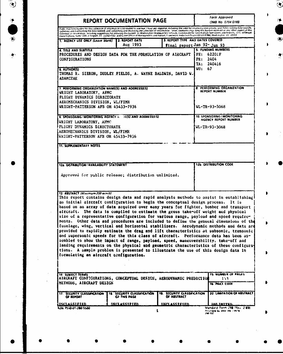
This report contains design data and rapid analysis methods to assist in establishing1an initial aircraft configuration to begin the conceptual design process. It Isbased on an array of data acquired over many years for fighter, bomber and transportaircraft. The data is compiled to estimate the gross take-off weight aud physicalsize of a representative configuration for various range, payload and speed require-ments. Other data and procedures are Included to defiat the genrwal dimensions of thifuselage, ving, vertical and horizontal stabilizers. Aerodynamic methods and data ariprovided to rapidly estimate the drag and lift characteristics at subsonic, transonicand supersonic speeds for the this class of aircraft. Performanc~e data has been as-sembled to show the impact of range, payload, speed, maneuverability. take-off dadlanding requirements on the physical and geometric characteristics of t .hese coinfigurations. A sample problem is presented to Illustrate the use of this design data informulating an aircraft c,.kfiguration.
AIRCRAPT CONFIGURATIONS, CONCEPTUAL DES$!CNif AEROI)TIWIC pREUlC'lIUNETHOUS, AIRCRAFT U)ESlGN tP%*
SU SCCuRITV CtASWeCATBON 19. SECURITY CLASWICATION 10. SECURItY CtASW6CAtIONt 10 UMITTION O ABS~tACTOF 0IPOiAt W TI4S PAGE OF ABSTRACr
1 IiiLa" IFI IIb mu[ k!t;In llft!TWlILVI1IM?1ti 1-i
IV 0 SQ0-W`% S1f0v 0i 09 0 0' 1 0
4
0 TABLE OF CONTENTS19)
PAGE4D
ID
1. INTRODUCTION 1-12. AIRCRAFT CONCEPTUAL DESIGN 2-1
3. IMPACT OF PERFORMANCE REQUIRMENTS 3-1ON CONFIGURATION SHAPE
4. DESIGN DATA FOR INITIAL SIZING AND 4-1SHAPING OF CONFIGURATIONS
5. METHODS AND DATA TO ESTIMATE PRELIMINARY 5-1AERODYNAMIC CHARACTERISTICS
* 6. INFLUENCE OF AERODYNAMIC AND 6-1CONFIGURATION PARAMETERS ON PERFORMANCE
7. PROCEDURES FOR THE FORMULATION 7-1AND ANALYSIS OF AN AIRCRAFtCONFIGURATION
& CONCLUSIONS 8-1
9. REFERENCES 9-1I
APPENDIX A REPRESENTATIVE OPERATIONAL AND A-IADVANCEMD CONFIGURATIONS
APPENDIX B VOLUME AND AREA RELATIONSHIPS B-I S.0...
APPENDIX C WINGS IN SUPERSONIC RLoW C-I
I m -. -. r. ,a ifI
O •4~j O I
LIST OF FIGURES
I
Figure Title Page
2-1 Concept Formulation 2-2
3-1 Impact of Speed on Configuration Features 3-2
3-2 Subsonic Aircraft Pressure Drag 3-3
3-3 Supersonic Aircraft Wave Drag 3-4
3-4 Aircraft Thrust and Wing Loadings 3-6
3-5 Parametric Performance Trade-Off Study 3-7
4-1 Payload-tRange Capability for Transports 4-2
4-2 Payltad-Range Capability for Supersonic Fighters 4-3
4-3 Length of Transports 4-4
4-4a Length of Supersonic Fighters 4-0
4-4b Length of Supersonic Fighters 4-5
4-5 Empty Weight Fraction for Bombers and Transports 4-8
4-6 Empty Weiht Fraction for Fighters 4-9
4-7 Fuel and Payload Fraction for Transports 4-19
4-8 Fuel and Payload Fraction for Fighters 4-11
4-9 Wetted Area for Transports and Bnibers 4-13
4-10 Wetted Area for Fighters 4-14
4-11 Airalln Volume 4-15
4-12 Airctdt Dy Weight Density Patanieer 4-16
iv
t.,•o
* • S 0 0
4-13 Wing Area and Wetted Area 4-18
4-14 Span Loading and Wing Loading 4-19
4' 4-15 Fighter Aspect Ratio and Wing Sweepback 4-20
4-16 Wing Sweepback Angle 4-21
4-17 Aspect Ratio and Wing Thickriess Ratio 4-23 •
4-18 Wing Characteristics 4-24
4-19 Horizontal Tail Sizing Guideline 4-25S
4-20 Vertical Tail Sizing Guitcline 4-27
5-1 Dynamic Pressure 5-2
5-2 Reynolds Number 5-3 0
5-3 Drag Prediction/Definition 5-5
5-4 Turbulent Skin Friction 5-7
5-5 Drag Build-up and Mach Number Effects 5-8
5-6 Fighter Drag Polar-Lift Efficiency 5-10
5-7 Drag-Due-to-Lift 5-11
5-8 Wing Efficiescy Factor 5-12
5-9 Trim Lift and Drag Procedure 5-14
5-10 Aerodynamic Cleannems of Aircraft 5-15
5-11 Minimum Wave Drag Bodies of Revolution 5-18
5-12 Supersonic Area Rule Concept 5-20
. t3 Transoaic Drag Rise at Mach 1.2 5-22
5-14 Transmw c Drag Cowation 5-23
V
• • •• • • •• •
5-15 Parasite Drag Area Correlation at Mach 2 5-24
5-16 Variation of CD0 with Mach Number 5-25
5-17 Subsonic Lift Curve Slope 5-27
5-18 Supersonic Lift Curve Slope 5-28
5-19 Maximum Lift-to-Drag Ratio 5-30
5-20 Subsonic Maximum L/D Correlation 5-32
5-21 Subsonic Maximum L/D Variation with Aspect Ratio 5-33
5.-22 Variation of Maximum L/D with Mach Number 5-34
5-23 Maximum L/D at Subsonic Cruise and MaximumSpeed 5-35
6-1 FLAPS Down CL MAX 6-2
6-2 Stall Velocity Versus Wing Loading 6-3
6-3 Take-Off Velocity 6-4
6-4 Take-Off Distance 6-5
6-5 Cruise Altitude 6-7
6-6 Impact of Cruise Fuel on Transport Range 6-9
6-7 Impact of Cruise Fuel on Fighter Range 6-10
6-8 Impact of Supersonic Speed on Fight-es 6-11
6-9 Specific Excess Power, G = 1.0 6-16
6-10 Specific Excess Power. G = 5.0 6-17
6-11 Maximun Sustaineo "G" CntuurM N1 = 0.6 6-19
6-12 Ntaxuimu Sustained "G" Contours, M = 0.9 6-20
6-13 Maxuinum Sustained *G-" CAontos M = 15 6-2)
vi
• • • •• • •
6-14 Thrust Variation for a Modem Fighter 6-22
A) 6-15 Aircraft Turn Rate, V = 200 - 800 Knots 6-25 Ag)
6-16 Aircraft Turn Rate, V = 700 - 1400 Knots 6-26
6-17 Luding Ground Distance 6-28
6-18 Descent Distance Over 50 feet 6-29
A-1 A-7D Fighter Configuration A-2
A-2 F-106 Fighter Configuration A-3A-3 F.-15 Fighter Configuration A-4
A-4 F-16 Fighter Configuration A-5
A-5 Advanced Supersonic Fighter Configuration A-6
A-6 C-141 Transport Configuration A-7
A-7 C-5 Transport Configuration A-8
A-8 Advanced Transport Configuration A-9
A-9 B-52 Bomber Configuration A-10
C-I Arrowhead Wings with Double Wedge at ZeroIncidence C-5
vii
• 0 0 0 0 0 0 0 0 0
Alf
Nomenclature
a Acceleration, ft/sec2
Angle of attack, deg
Ax Frontal projected area, ft2
AR Aspect ratio b2 ISf
AWET Wetted area, ft2
b Wing span, ft
I for M>l
= --M 2 for M<
c Chord length, ft
F" Wing mean aerodynamic chord, ft
* CD Drag coefficient
CDO Drag coefficient at zero lift
CDP Pressure drag coefficient
CDTr Trim drag coefficient
CDW Supersonic wave drag coefficient
C IFriction coefficient
Cfe Equivalent friction cfficient
CL Lift Coefficient
CL Lift curve slope, I/deg or l/cad
CMAN Manwuver lift coefficient
CIJ.A Maximm useable liWt coaffcmient
viii
* 0 0 60 0 0
II
CL1o Lift coefficient at take-off
CR Wing root chord length, ft
-CT Wing tip chord length, ft
d Diameter, ft
de Fuselage equivalent diameter, ft2
& Deflection angle, deg
Horizontal tail deflection angle, deg
DLF Design load factor, g's
e Wing efficiency factor
f Equivalent parasite area. ft
FF Form factor
g Acceleration due to gravity, ft/sec 2
y Glide slope angle, deg
GTOW Gross take-off weight. lb
h Altitude, ft
IF InterferencC factor
I
K Drag due to lift factor, K- xARe
L Fuselage Length. ftor Lift. lbs
LE Leading edge
I Wing taper ratW. CrCR
A, AtE Wing leading edge sweep angle. deg
I
ixS
* 0 0 00 0
A Ac Wing quarter chord sweep angle, deg
) IJD Lift to drag ratio
lir Horizontal tail arm, ft
lV-r Vertical tail ann, ft
M, M. Mach number
n Load factor, g's
q Dynamic pressure, lhft2
R Radius, ft or Range, nm
Re/ft Reynolds number per foot
p Air Density, slugs/ft3
SFC Specific fuel consumption l(udlbOO,•hr)
SORO1jM LandingfTake-off ground roll distance, ft
*MT Horizental tail area. ft2 0
y Density Ratio. PAL"
PSL
SL Sea level
Sx Reftmattc area based on frontal projewted ar, fO2
$m Wing rekerenwe ara. fte
SVr Vertical tail amrea, fi
Sw.. swtý. Wing area. ft0
Sa We-WettCd a. a,
Wing thickaUss. ft
* S 0 00 0 0
T Thrust, lb
t/C Wing thickiess to chord ratio
40 Turn rate, deg/sec
T/W Thrust ic weight ratio
ULF Ultinate IoM-, fiactor, g's
V Velocity, k. 's
V. Vo Volume, ft
VAM L= .i ?proach velocity, knots
VSTAII S•" velocity, knots
VTQ. Take-off velocity, knots
W Weight, lb
W/b- Span loading, lb/ft2
WEMpri Empty weight. lb
WFC, \VWKiu Cnuse fuel weight, Ib
WF.IJEL Fur! weight, lb
WiL Payload weight. lb
W/S Wing loafing, mrft
•O lTak-Otff weight. lb
( ).,l• a l odiuons
• • • •• • •
FOREWORD
This report was prepared in-house by Thomas R. Sieron, Dudley Fields, A. Wayne
Baldwin, and David W. Adamczak of the Aeromechanics Division, Flight Dynamics Directorate,
Wright Laboratory at Wright-Patterson Air Force Base, Ohio 45433-7913. It presents a
compilation of design data acquired over many years in the development and analysis of
advanced aircraft configuration concepts. The work was accomplished under Project 2404, Task
16, and Work Unit 67. It was prepared during the period January 1992 to June 1993.
The report is composed of eight sections with a sample problem contained in section
seven. The sample problem presents a procedure for using the design data and aerodynamic
prediction methods in the formulation and analysis of an aircraft configuration. Appendix A
provides a handy reference to obtain geometry information on current and advanced aircraft.
Appendix B contains mathematical equations to compute the volume of simple shapes, such as,
cones, bodies of revolution, and cylinders. Appendix C contains fundamentals of wing wave dra
in supersonic flow.
p
xii
p
f. 1. INTRODUCTION
t'he development of aircraft configurations is both an art and a science. Most beginning
designers s=ar out with a background in aeronautics and learn to understand the basic functions
of airplane components. These include the fuselage, canopy, wing, engine, inlets, nozzles, 0
horizontai and vertical stabilizers and control stufaces. Instructions in a text book are then used
to configure an airplane and evaluate its basic performance capabilities. As the designer acquires
experience the formal process tends to diminish and is replaced with knowledge and skills
learned in the practical design of airplanes.
This report provies design data and procedures in an attempt to fill a gap between the
seasoned designer and inexperienced designer. It is based on an array of data acquired ov'er
many years in the design and analysis of various types of aircraft configurations. This empirical
* data base can be used in the initial sizing and shaping of a configuration to meet some specified
performance requirements. These performance requirements generally consist of cruise rangt,
maximum speed, payload, maneuverability, loiter and take-off/landing field distances. Other
requirements may be imposed but these axe the primary ones for most military aircraft
configurations.
The report is intesided to augment aircraft design textbooks such as Nicholai and Raymer
(Refewces I & 2). These textbooks contain a systematic approach to the preliminary design
of aircraft configurations. They am very valuable to engineers in understanding the airplane
design proces&
Th1 rapid advaucenumt in computer technology has created a revolution in the design and
antalysis of airraft configuration. It is not unusual to have a worksW-tion for each enginwer with
-1~~
* 6 0 • • 0 • 0 •
access to numerous computer aided design (CAD) programs. Computer analysis programs are
1 available in the government and industry for each technical discipline, such as, aerodynaiv -s,
structures and propulsion. In addition, design synthesis programs are available which combine
these single discipline programs into a completely integ.-atec program (Reference ' and 4). These
design programs contain geometry development subroutines as well as subroutines for each of
the technical disciplines. These subroutincs art. coatrulleki by a cer tral executor. The executor
controls the problem and routes the information t3 the various subroutines, as required to solve
the problem. These design synthesis programs car. be used to perform rapid configuration trade-
off studies and converge the design te mee+ specified prfcmri&ac requirements.
The continued advancement in computer size, speed and storage capacity should
drasically reduce the time required in the design cycle and permit the development of more
optimum configurations with higher performance. The emergence of computational fluid
* dynamics (CFD) as a design tool will expedite the design cycle by reducing the amount of ti ie ie
required to validate and verify the airplane design. Today the configuratik, is defiiwd using a
combination of linear theories. semi-empirical methods, CFD and wind twnltels testing. In me
long term (10 to 15 years) it is envisioned CRD will be used throughout the design, and wino
tunnels will be used only to spot-check the final airplane design. These developments will all
enhance the design prcess and produce a higher quality airplane .,,in less time... znd at re-duced
costs.
1-2
2. AIRCRAFT CONCEPTUAL DESIGN
The evolution of a new aircraft concept is generally based on a set of performance
4 atrequirements. The design engineer must depend on background and experience to formulate the
initial configuration in search of satisfying these performance requirements. The cycle between
the initial concept formulation and the final configuration, which satisfies the requirements, is
known as the design process.
This report is intended to assist in establishing the initial configuration concept in the design
process. Past data are provided to estimate a gross weight based on range, payload and speed
requirements. The gross weight can be used to determine the physical size of a representative
configuration. Other data and procedures are included to define the general dimensions of the
fuselage, wing, vertical and horizontal stabilizers. These inputs are required to begin the analysis
and design process.
The process was previously performed by individual analysis programs, but with the advent
of personal computers and workstations it has become fully automated. Today, vehicle synthesis
programs are availabli; which perform the entire conceptual design process. This process is
depicted in Figure 2-1. Major features consist of sizing algorithms, aerodynamic, weights,
propulsion and performance subroutines which iterate until the concept meets the specified
performance requirements.
A program used extensively by the Aeromechanics Division is called the Combat Aircraft
Syndh'sis Program (CASP). a robust program applicable to a wide variety of aircraft. CASP is
a computer code for the conceptual design of military fightem, bombers and transports, plus their
variants. It use a basic g*xýmetric description of a vehicle to generate a detailed aerodynamic
2-1
* S 0 0S S S
0 and weight analysis using Datcom type methods. (References 5 and 6).
The aerodynamic analysis is a first level calculation for lift and drag based on the Air Force
Datcom handbooks. The calculations include lift curve slope, lift at zero angle of attack,
maximum lift and maximum angle of attack. Drag calculations include skin friction drag, wave
drag, camber drag, drag due to lift and trim drag.
The weights analysis is a first level mass properties methodology which outputs estimates
for structure, propulsion system, and useful loads, plus systems and equipment weights. Methods
in the analysis are based on the specific type of aircraft being studied, a user input, and additional
inputs of payload weight, basic engine weight, maximum dynamic pressure, ultimate load factor,
and gross weight estimate. These inputs axe used with the geometric description to calculate
mass properties, fuel weight and a check of volume available versus volume required. A mission
analysis subroutine uses the calculated aerodynamics and weights from the input geometry. The
user has to supply a mission using different segment options (Acceleration, Climb, Cruise,
Combat, Landing, Loiter) and the engine propulsion deck (thrust and fuel flows). CASP will
then run the given mission and output the mission segments in a detailed printout. In addition
to basic mission profile results , CASP can also be tasked to optimize the overall mission for
specific payoff functions. The user may choose to maximize loiter time, radius, or number of
combat turns, or to minimize the aircraft gross weight. CASP runs on an IRIS workstation and
takes less than 30 seconds to run a basic aerodynamic and weight analysis, while a complete
mission and optimization of a mission takes only several minutes of computer time.
The arrangement and blending of the configuration components is still a challenging task,
even with the assistance of rapid computers and friendly software. The designer needs to have
2-3
0 0 S 0 0 0 0 0 0
a thorough understanding of the impact of performance requirements on the configuration size
and shape. This knowledge -nd experience permits the injection of innovative ideas into the
vehicle design.
2-4
• • • •• • •
3. IMPACT OF PERFORMANCE REQUIREMENTS ON CONFIGURATION DESIGN
An experienced designer can view a new aircraft and make a reasonably accurate
evaluation of its performance capability. This ability is based on an extensive background in
aeronautics and indicates that individual configuration features are related to the performance
requirements of an aircraft. A thorough understanding of fluid mechanics, performance and
propulsion coupled with general knowledge of structures and subsystems is therefore a
prerequisite to being a seasoned designer. The most important performance parameters are speed,
maneuverability, range, take-off and landing distances and useful payload. (References 7, 8 and
9)
The speed of an aircraft determines the primary appearance of a configuration. A
subsonic fighter and a conceptual supersonic interceptor are illustrated in figure 3-1. A number
of other aircraft are also displayed in Appendix A as a convenient reference. Subsonic airplanes
are characterized by low fuselage fineness ratios, blunt nose and wing leading edges, short
fuselage nose sections and large protruding cockpits. Subsonic aircraft typically, have fineness
ratios in the range of 5 to 7 to minimize subsonic pressure drag and maximize internal volume p
as shown in Figure 3-2. There is only a minimal decrease in pressure drag beyond these fineness
ratio values. Supersonic cruise airplanes have high fuselage fineness ratis, sleek nose sections
with the canopy blended into the fuselage, high wing sweepback with low thickness ratios and
low wing aspect ratios. These features are dictated by the need to keep profile drag at the lowest
possible level. Figure 3-3 displays transonic wave drag as a function of fineness ratio. Fineness
ratios of 8 or higher are required to avoid large wave drag inceases.
The maneuverability requirements of an aircraft are very dependent on its application.
3-1
p 40
*
117V
*.......... *I -i--IeN
• .... • . 4 . * . . L . * . . . I . . L . J . . * . . L..... ...... L. ..... L. . . .. . ..... .... ....... .... .. .. . . . . . . . . . .
. . . . . . L.. . . . ................
S.. . . . - , --- ,--- ...........,.-.. ., .. q .. -.. .... .. ., .... .,..........,.-. ... . . - . .,. . ..... ,
- 4 - 4 .4-- . V- 4
Sa
.. .. . . .. .... . . . . . . 1 1 : . . . .
, , ,.....: . . . . . . . ,i,..
; • - - . • . . .. . .÷ . . . • . . • . . .; • . .;;... . . .. . . . . . . . . . . . . . . . . . .
-------- L .....-...----- r-4-----1
, ,. , ,. .-- , . +...- .... ,--- ----- ---- ..... - , .... ..... .... ...... . . .............. .... k 0
4 ............. ... ... .. ... .. .... ....... .. ....... 4-- .... - { -- !- 4- .e --- I -- ---
00
- 0
: . .. . . : . . . . . . : . . . . . . . . : ........ ..... . ..... .... .. ..... L . ..... .... .... .... . .... .... . .. .
- ..-- h -.--.. . .-... . ......... ----- -
I. 4........ ... " . ..... - ...... .. .
.;-.,; ~~ .- ,.-., .4 . . ... . .... ... ... ... -A....... •I � " "
.. . . . . .L. .. .. ..... ,.,L, ... . .... .... .. .. . . ,. , ; . .. ,, = , . . , , .... .. ..... . .... ...... ..... ..... .. .... ... .. . ...... ....... . .L. .. .. , , .... ...
-. .. . . . . . . .. . . . . . ...
N S .*........ .. 4... 4. .. 4'~ ... -..-. ....
* . . . . . ..... . ... . . . . .. ... .. . . . . .. . ... ...... . . . . . . . . .4.. . .N- 4.5 - . .. ..... .... ... % 4 4 . 4
9 =ra osas@~(urvio9 OINOSfiS 00
3-3
• • • •• v •
S~p.~ .... ..... ... ------.... ............
........ ................ L......... .... 1
................................................... .... 0............... ........4 . ~ . .... k....... I .--
* . ... J. U .. t..J... S... h... .... L...4....... J. .. U
............,........ ... 1 ',-7 ............................----- -- - -- --- --.. . ..... ....
................................................................
11 -- 7 - ..I ..1. . 1- - . . ....
.. .... ... . . . . . .
3.4
. .......
.. .... . .. .. ........ 0 0
Transports and bombers generally have very low maneuver requirements. Representative
maximum load factor values are between 2.0 and 3.0. This permits these aircraft to have
relatively high wing loadings dictated by fuel load and take-off and landing. Typical ranges of
thrust and wing loadings are presented in figure 3-4. A typical transport has a T/W = 0.25 and
W/S = 110, in contrast to modem day fighters of T/W = 1.10 and W/S = 75 Fighters are
designed to engage in air-to-air combat and require a very high maneuver capability. The
maximum load factor is 7.33 for the F-15 and 9.0 for the F-16. Parametric trade studies of
performance characteristics are conducted early in the design cycle to arrive at nominal values
of T/W and W/S for each airplane. Figure 3-5 shows the impact of maneuver, acceleration and
take-off distance on the gross take-off weight as a function of T/W and W/S for an advanced
supersonic fighter. Each individual requirement imposes a different set of T/W and W/S values
and these type of trade studies assist in establishing a final set of configuration requirements at
minimum gross take-off weight.
The range or radius capability of aircraft is directly dependent on the lift-to-drag ratio
(L/D). This is the true aerodynanmic efficiency measure for aircraft. The LAD is directly
proportional to the wing aspect ratio and the cleanliness of a configuration. The drag must be
kept to a minimum in all speed regimes, and the configuration shalped #,- ovoid flow separation
at cruise conditions. Wing sweepback angle is generally a compromise between rnge. speed,
and maneuverability. The advent of superwritical wing technology penuits higher lift for the
sante aspect ratio wing and thus higher L/D's. The range mcquirement also influences the
fuselage size since fuel is genorally carried in fuselagge tnks as well as tle wing,
Another pefoznuzince ptrameter which influw-ens the configuration shape is take-off and
3-5
• S 0 0 0 • • 0 • 0
.....4. .............. ..... .... ..... 4
~ . .. .. tJ ... ...... .. ..
"-4.... --4 t-
I*- N,. . .... ..4 11----
.. ... . .. . .. . .... ... .. .. . .. . .. . . ...
.. .. . . .. . . . . . **. .. . .. .
bCu
LII ..
Goo
30 3M Swi a,.alI.- ,su 0alvSwwvp
P .- -3-6
..... .......... ................ .......... .. ........ ............... .
4f S. .. .. .. . ., .. .............. ...... ... .. .. ......... ...... ,.................. •"............... -- -..... .... ....
-i a~~~~~ ... .. . . . : . . . . . . . . . . . . . ....... ....... .• ........ .. ...... .... .. ...
S.......... ... .............. . -•.. . .. ;e....•• • • -• " ... ....... .... • .... • .\ " '........r ...... . . . . . ... ... ..:
.. . ........ . . ........... • ........... I-. ..... \..... - ./.... :..... i: • ....... -- -- ....... ........--
S..................................................
... .. .. .. .. ... ........ .. • .........S.. . . ' •8 , , . • / i . ... .... ,........ .. .... ......... V " ... .. .. ........ ... . .. .
.. .. .. . ........
N i•..
N1l001) MOO.L
3-7
landing. The speed at take-off is directly proportional to wing loading and inversely proportional
to the lift coefficient. Thus the designer must also Consider the length of runways in determining
the size and geometry of the wing. High lift devices can be used to augment the lift of the basic
wing during take-off and landing.
Payload is the useful load an airplane can carry and deliver. This is perhaps the most
meaningful performance requirement since it is the ultimate reason aircraft are built. Payload
consists of crew, passengers, cargo, guns, bombs, missiles, etc. Cargo weight and density drive
the payload bay size and are directly related to the fuselage length and diameter. If air drop of
equipment is a mission requirement, this strongly influences the aft fuselage design. In fighters,
the primary payload is missiles, bombs, and guns. These weapons may be carried either
internally or externally on the aircraft. External weapons need to be fully integrated with the
underside of the airplane, if low drag is a goal. Internal weapons require larger internal volumes.
Internal versus external weapons carriage assessments involve many factors such as mission,
speed, vehicle size and cost, and typically require design details beyond the level addressed in
this report.
The above discussion illustrates the impact of various mission requirements on the aircraft
geometry. It also is to be noted that some components are influenced by two or more
requirements. This mandates that the component be optimized considering all requirements. This
is the task of the airplane designer in developing the most efficient design.
3-8
0 0 0 0 0 0 0 0 0
4. DESIGN DATA FOR INITIAL SIZING AND SHAPING OF CONFIGURATIONS
The physical size and shape of an aircraft configuration is dependent on the performance
goals established by the customer or using organization. Appendix A displays pertinent features
and dimensions of several past, present and advanced aircraft configurations. A parameter which
can be used to correlate the size of an aircraft is known as ton-miles and combines range and
payload requirements. It can be used for both military and commercial aircraft. The gross take-
off weights of numerous subsonic aircraft are shown as a function of ton-miles in Figure 4-1
(References 10 - 13). The payload of the aircraft is divided by 2000 to obtain tons. This is next
multiplied by the range of the aircraft to obtain ton-miles. A large increase in ton-mile capability
can be seen as the gross take-off weight exceeds 500,090 pounds. This same parameter can be
used to correlate fighter aircraft, as depicted in Figure 4-2. A band is used for this type of
aircraft since fighters tend to have more diverse performance requirements. These design curves
provide a rapid method to estimate aircraft initial gross take-off weights based on payload and
range requirements. The gross take-off weight is defined as:
rVTO = WEMT,, + +,• , WPA YLOA D
The length of an airmcft is very critical and depends on gross take-off weight as shown
in Figurus 4-3 and 4-4a. "llTe driving performance requirement is cargo size and weight for
trmspors and mnaximum spied and maneuverability for fighters A factor which must also be
consdcred in aircraft length is the size of availab;e mainterance hangers and protective shelters
to maintain and prot, the aircraft. There is excellent corrlation with gross take-off weight for
translxrts and moderate agntnit with fighters. Tlhe fighter condation can be improved if the
cmpe y weight is known as shown in figure 4-4b. In cither caw. the data provides an initial
4-1
* 0 0 • • 0 0 0 •
.......... .............. ...........L L -- -----
.... .... .... .. - ---- -- --
7-4 -..... ..... -T ------------------- 4----;
-.. .. . .. .. ..4 ...j . . . . . . ... . .. .. . . . .. . . .I-- - -4
S.4-.------------
jr~ .. .. .. 01--I. . - .1-- - . . .0
4 . 2 .... J - I-.. J .A ....... 2
........... . .. ... . .. .. . --- -- .- -
104
--------- --- --
.. I .. . .. 0.
..... ..... ... ..
---------- x... suoj --- p--og......4-2 ........
---- -- ---- - --- --- ---- --- ---- --- ------- ---
0.... .... ... ...... 0.0..0.0
. . . ... . .
I - - - . . .. . . . . . .
-- - - - - -- - - -
--- C- ----------------------I .. ..... ....... .. ...... ... ...... .L--- -- --- ------
... .. .. .... .. .. ...... .. .. -- ---- -I -- 4
........ ..............
.. .. . .. .. -- ------ --- ...... .. ..... .....
------ ----- -----.....
. .... .. .. .... ... .
QSUDIJ x SUOJJ iqLOlu
R-3
.. . ... . . . .. .. . . . .. .. .. . . . . .. I ..
*-------------------- 1--- I,------ 4------------4 I%--
* -4 4 4 --1' . .........
............. r-- --- - --
-------- --------- - ----------- -7 T_
:- - -- -------_--_--1-f-----1 ----I---v--------f- - :--
------------.------
.......... -----
o.....0 . 0....0..0.0... .. .. .. .. ... . .. 0..-0.. .
.. ....... ...... .
4- ~ ~ (w 4qgur ....... ..... .......
. ... ... ... .. .... .. .. .. 4 -4--4-4
-7 . . .. . . .. .
* 0.....0.0.0.0.0
.. .(i ....
...-.. ------ --
- -- - - - - - - -------------.. . ,-----. . ,
- - - -- -- - - .. .. ... .. ------------
II-- - -- - --- -- ---- -
-- I--- - -
.... ..- . .. .- -- -- I -----
----- ---- ---- ----
46: 0
-- --- - -h- - - - - . ... . I I ..
. . ... . .I - --A - -- --
*- -
.. . . .. . . . ........ .. . . . .. . . . I -- - - . .. .I .
.. .. . . .. .. .. L0N
.. .. .. .. q..u.
... .. .. . ... I - 5
... . . . .. . .
* 0 0 ..0.0.0.0...
I
, . . . . . . . .. . . . J . . . . . . . . . . . . . • . . . . .. ... . . ... . . . . . . . a . . . . . . . . .. . .. . . . . .. . . .
4> It
--- --- - -_ -
------- ---- ------- --- I ------- - ---------- I ---- ----
j -- - - - - - I -- - - -- - -- - - -- -- -- -- -- - - -- - - -- --- -- - - ---- ------
+~ -- --------------.-----------. -....... + ....... .. ......... . . ..-.. .. - I , I ------ .... ... I . . ..I -- ---- - -I .- -
-- -- --- --- --I, .. ..1 . 1 ------. . . .
, I *
- a - a -a - - -- -- -- -- ----- -
4-6
-~1.
• • •• • • •• •
starting point and may be changed as the analysis progresses.
Empty aircraft weight is often considered more important than gross take-off weight in
estimating cost. The majority of cost estimating relationships use empty weight for Research,
Development, Test and Evaluation costs. In general, empty weight includes all aircraft weight
except fuel and payload.
Empty weight fractions are presented in Figure 4-5 for transports and bombers. Empty
weight fractions decrease from 0.55 for transport aircraft weighing 100,000 pounds to 0.44 for
aircraft weighing 800,000 pounds. Bombers show a similar trend with GTOW with a nominal
value of 0.35. In general, bombers are designed for very long ranges and require more fuel than
transports. Also the payload requirements are small in comparison to transports. Typical
payloads may range from 20,000 to 40,000 pounds.
* Empty weight fractions for fighters are higher than transports because of maneuverability
requirements. As noted earlier, fighters are designed to fly up to 9 g's. This requires a much
heavier structural weight to withstand the flight loads. Fighter empty weight fractions are
presented in Figure 4-6 and range from 0.72 at low GTOW's to 0.65 at GTOW approaching
60,000 pounds. The agreement of the design data for past and current aircraft is surprisingly
good and may be used with a high degree of confidence.
A corollary to the empty weight fraction is the fuel fraction and payload fraction. It can
be seen from Figure 4-7 that the fuel fraction and payload fraction increase with gross-take-off
weight for transports. In transport design, many times more fuel will be carried in exchange for
payload depending on specific mission needs. In fighter designs, the fuel fraction varies from
0.25 to 0.30 depending on gross weight as illustrated in Figure 4-8. The payload fraction steadily
4-7
•* 0 0 0 0 0 0 0 0 0
- - - ---- ~ --' -4 -----T----I----- -----I------
------- - ---....... .... ...... ....-
4 4 1 - - ---4- -- -- ----- 4 00
- ---- -i - -- - - - - --- ... -..
r- ---- -----4 -.00 . ......
-- T -- - - - - - -...-- -....r--A4--- ...-- --- - - - - - - - - - - - - - -----a - -- --- -
---------------------------------- -------------------------
-------------------------- ,
S--- - - - - - - - -- ------- - ---- r--
- - - --- ------
a - ~ -- %..,S - - - .. ~ -------- ---
--------- .. .. I I -- --- - --- .... .... ......----------_ -- - -- - .. . . . . - _ - -
0_ .. ... ... . .. ... . ... . .. .. ... ..... - _ --- -
r 0 ------------------- ---- .... .... 0 0.0
--I -- --.. .. ... ... .. .... .. . .. .. .. ... .... ... .... ... .... -8- -
... ... ... --- --- ... . .... .... - ...... ...
... .. .. .. .. .. ..............
------------ ---I -- ------ I.,--- -- .. .. ....... ....... -- --- ---
----------
. . . . .. . .. .. . . L . . . . - - - - --- -- - - - - -- --- 0-*----------- ----- r - -- -- - -r - -- - - - ---- - ---~ - --- I4 -
.........I. . ----------i- - -- -- - -- "--- - -
4; ~ ~~~ ... .. .. ..---- ---- -- - ..... -----L- --- --
--- - - - ---- --- -- - ----- - *--- I
..... .... ..... ....
- - - - - - - - -- - - -- -
--------- I ------ - ------ .......
. . . . . . . . .
.. .. .. ........
0. ... . .. ... . .. .... .. ......... - ~.... 0.. ..0.... 0..
.... .. . . .. . .. .... ...
. ... ..... ..
...... .. -- -----00
o------- .... ..
~~~~------ ----------- ---------- ------ I----... '--
- - - -- - -.. ..I
-- - -- - - ---- ---
. . . ... .- -- - - . . . .. . . .. -- - -- - -- --
- - - - - - - -- - - - . ... . .- - -
. .- . . . .-. -
.... . . ......---
---- .... .... .. .. .. .
o- ----- .........o. . --- ......-----
SUOIP~d PU20p(U9 put? I~nd
4-10
-4 ,- - - - ----- -- ------- -- 0-------
-------- ------- ------ ----
0
-- - - - -I -- ---- .... .
. . . ... . -- - - - - .. . . . .. . . .
*- -- ----- -- 0
-- ----0. .. .
-----s~ ----~u -U .... .. ..
... .. ... . .... ..4..11.
.... .... . 7 1 .. ...
*2 -- I .. .. . ........ 0
increases with gross take-off weights up to 60,000 pounds and permits a larger payload to be
S)delivered on targets.
A useful design curve is the wetted aiva of an aircraft as a function of empty weight. The4'4,
data for transports and bombers are shown in Figure 4-9. The average weight per square foot
of wetted area is 9.25 pounds for cargo planes and 10.4 pounds for bombers. Thus once the
wetted area is known, a check can be made on the empty weight or vice versa. Data for fighters
are presented in Figure 4-10. There is a little more scatter in the data for fighters because of the
more diverse maneuver and landing requirements. The average weight is 12.7 pounds per square
foot. This increase in weight is related to the higher load for fighters.
The wetted area and volume of various aircraft were correlated by Caddell in Reference
14. This data, supplemew'..d with additional aircraft by the authors, is presented in Figure 4-11.
There is a surp ising consistency of the data, and the curve fit equation A wv7 13.6 (V)0 .688 is
very useful in sizing the initial configuration. Appendix B contains several volume and wetted
area relationships for bodies that are easily defined mathematically. such as Sears-Haack bodies
and ellipsoids. The importance of these relationships cannot be over emphasized in the
fornulation of configurations,
Aircraft density is an interesting prtutneter to correlate the structural and empty %vight
of various airerall, liniply weight was found to corrlmAte the data better thai• gross taIe-toff
weigiht. since the fuel d&nsity (48.6 pixnds jx-r cubic toot) is very heavy in wointrar, s to the
average dry density of an airnctufl. and ditftkn¢lt amounts of fuel arm carriet by cacti aircraft. The
dry density parameter is displayed in Figure 4-12 as a variation with mptly weight. Tlis
infonnatiotl can bc used as a chexk on aircraft volume and provide additiwtal "nfide•nx in t11e
4-12
0 0 0 S • 0 0 0
--------- -------- r - ...... 1 .............
..... ..... ...... ... .............. ................6..
.... .... .... .... ..
* I I ' ------ ---- - ------ I-- -- ----- I- ~ I . '
.- . . .
, .* w :I
------------------- -r. , - r----------, '
.. .. .. . . ------~' 1 4 . . L ~ . -- 1*
. . . . . . . . . . . . .... I.. t..-- - - -
C9-0
---------- 'I'
.........
--- .. ................
.. .. .. . - --
(Yuoof eaz pafl);;
4.14
------------•L ] ]• 2• •]]I] ] I• ]•L ...................... ..... ........
:.- - - '• -& .. . .. 4 .. .. 4 .. ... . .................'' ' ' & - ' ' ........." ° ...........: : : : : : :: : 00 : m-
i--!--,:---!---•------------- ----------• . . . ..". . . . . . ..... .. I-: - - • - - -.. .... 4 ...... • . . . ..?. . . .. . . "
*-------------------------------------- --------------- ~-----.........
..... I-------
". .... ..... .. .. -- .. . . . .!. . . . .i ............
........ ........ ...............---------- ,. ...i .. .. .* ......... . . . ......
S4-j
- * -.......... I.. ... .. ,*~~~. .........99 9 9 9
4-15
• • • •• • •2
d S...........................................
*. ............-- --........ .....I.. .
".... ............~
.. . ... .I . .. I.. - -...
C 04
- ~L . L.... . ... .... ..... ...J..LI ......- -- 4 -----. J.5
-- i-1----l------------------ ------- 4
*----------------------------------------------------------
* ) % . -%-4 * j. A .4 A--S -' ~.%S ~ -- 4.. .... ................ .0. .
..... ........ ............. -7 .. e7
ItI
OWa.
16I
configuration concept.
The wing area of transport and fighter aircraft can be estimated from wetted area using
Figure 4-13. This data has been compiled from a host of aircraft and relates wing area to wetted
area. It is informative to observe that fighters range between ratios of 4 and 5 and transportsS
between 5 and 6. Obviously, the above procedure can be reversed. The wetted area may be
calculated once the wing area has been defined from other sources. This frequently occurs when
estimating the total skin friction drag on a configuration.
The wing geometry and area are extremely important in formulating an aircraft
configuration (References 15 - 18). The wing loading parameter, W/S is obtained by dividingI
the aircraft weight by the wing area. The span loading parameter, W/o2 is obtained by dividing
the aircraft weight by the square of the wing span. These parameters dictate the range and
* maneuvering efficiency of an airplane. The aspect ratio of a wing relates the wing loading andAR WIS b_
span loading: A WI - b. A parametric curve illustrating this relationship is presented inWlb 2 S
Figure 4-14. Various aircraft are displayed on the plot. A close study reveals that fighters have
an aspect ratio range of 2.5 to 3.5 and transport aircraft between 7.5 and 8.5. These are values
that need to be remembered since they can be used as initial estimates in most aircraft designs.
The wing sweepback angle is shown as a function of wing aspect ratio in Figure 4-15.
Most fighters range between 40 to 50 degrees. This is a compromise between low speed cruise,
transonic maneuvering and supersonic speed requirements. The design cruise Mach number for
several aircraft is illustrated in Figure 4-16. It is instructive to note that as the cruise speed
exceeds Mach 1.0, there is a sharp break in the sweepback angle and it gradually increases to a
value of 60 degrees at Mach 2.
4-17
• • • •• • •
* 0 0 0 n 0 0 p - 0
Op
! ', .. . .. . _ .. ... . ...... . .. .. ... .. . .. ... . . . . . . ... •_ •.... ...... .... . .. .. ........ -- --............. ........ -----I , , , , S5 5 I S , S
i--r-* --t---•-------- --------• . . .•. . . . .1. . . . . . . .--- - -- - *- *- .. . ..... r...... I ---------- I - ---------------:....'... ... L.. .-------- ....... -- -- - -- -- --- -- --- -
-- -5 , , ---- --- --- -------• -- - T " ...--. .. ..--.. . ...- ... . . ...... ---- --- ---- -- -- -- -- -- I... -- ...... I . . . . : .. . . . . . .o . _-----------..-----....--.... ....- ...... . . . . .F ~ .... ...... 4 --- --- --- --- --- --............... --
, -, , ..-; ---.. -- -- ... -- --- -.. .. --...... ..---... ....... .... .. i-• -- -, --- ----,-r ------ I . .... ...... I... .. .. .. ..
...... - -- .. .. ..... •.. . ... ........ .• . .. . .. ... -- --- -- --- - -'- --- . .... ..... ............. . ... L ---- --- ..........----
--- --- , --- I.. .. ..
...... ..... ---------... ...... ..... .......... i..... •• !i---------------
- -, .. . . .... ... .
-- - - -- - - -I S.. :- _4 .. .., ,.. . .. - -- --,-
4-18
• iJ• • ••
-- - - - - - - - - - - - - - -------- --- --------- -- ------- -- - --- .....
7 : : : , :1
------------------------
I ~- ~ ---- 4 - a--
I -- .4 --- '- -4 4. *~1 - * - -- 4 ~----4-
r -- -1- . --- T---9- -- I-a....-...
444
---- --- ---- -- --- ----T4,0
I* 0
S.. . . .•. . . . •. . . . . . . .i. ...... i ........ ........ f ...... i......... ! ........ ,.. . .. .!........" * a |a a
* I * I I I
S... .... 1- .... . • .... .. •.... ... " .. .... .F .... .. " .... ...--... ... ....... .. ...... .... " ... ... ..... ..... . . . .I ----• ----- -------- f ........ I ........ - f --------
', ', ', I ', a a , I I'
----. . . . ..... . . --------I ---- ---- I, -- -- - -- - --- -- -- -- --- - ,, --- -- -- - --- -- -
L ----------------- -.. ... .•. . . .......... ',......... L ........ L --- --- -- --- -- " - -----. " ........ ........ --------.
. ... - . . ........ .... , ----I- --~~~~~~~~~~-- --.. . . .. .. ..--.. . .--.. .. .--.. . ..--.. . . , . .. . ...... ., ...... • . .... -- --- -------- --------.
........ I- ---------I- ---8 -...... ....,,........ -- -- -,, .......... ,........ ,....... ,,,
-- - - --- - - - .. .. .... ... I .,... . . . .I
, ....... . .... .. . .... . ------ -----
Va'-
I ........ ... .. I -- -- ---• . ... ..
',........ ,........ ....... I ....... i.... ...-A .J I•,, • ;....... ,....... ----- -- -- --- -- ---- ---
..... ..............".i! i:S.. . . . ..... . . .... . ........ .. .. .... ....... i-- .- - - - - -------------.--.--- -----.- --------. .. . . . •. . . .. ,. .. . . . .. . . . . . .
.~ ~ ,...... ........ --- -- ........ ,,........ ........... . ... .. .. ,. ...... ..... r ........ ............ |
.. ....',. ..', ... ... ... .
.. ....... . . . ..a..... .
............ ........ .•"........ .. •... ... .. .. ........ .. .. ........... ...
* ri a i i i a !
(gap) al3uV •4ovqdO2AS U.!A&4
a g a a a a a a 4 - r0
a a a a a a aa a
* a a a a • a a
0
* 00
-4-44
- . - --------------------------------a--------- ----- -0- -a-------
---- ---aa ----- a---- - ------------
* - 4 - I----------------------------
- - - - -- - -- - --- -- - -- - - - - - - - - --.. . .. . .. . .. . - - -- - -- ---- - - - - - - - - - ---
00
(Sop) aOjSV ipuqdoo&k SUIA
4-21
Another critical wing parameter is the thickness ratio. The higher thickness allows more
fuel to be carried internally in the wing but will result in increased wave drag at transonic and
supersonic speeds. Thus, the thickness ratio must be tempered if the airplane has a supersonic
speed requirement. This is discussed more extensively in the next section of this report. Figure
4-17 shows a range of thickness ratio values for both fighter and cargo airplanes. Fighters tend
to be around 5 percent and transports in the range 10 to 12 percent.
A design curve is presented in Figure 4-18 to rapidly configure a wing, based on wing
area, wing span, wing root chord and wing taper ratio X. It may be used for rectangular wings
(X =1), delta wings (,=0) and for the more common trapezoidal wings.
The size of the horizontal tail in initial designs is estimated from tail volume coefficients.
This coefficient is defined as:
1HTSHT* Carr----CS Wing
Data from previous aircraft are presented in Figure 4-19. It can be seen the relationship is linear
and corresponds to a nominal value of CHT = 0.267. Through a 3-view layout of a conceptual
configuration a nominal value of the distance from the horizontal tail quarter chord to the wing
quarter chord (lHT) may be estimated. This permits the determination of the horizontal tail area.
If a drawing is not available, a representative horizontal tail area of 15 to 20 percent of the wing
area may be used at this stage of the design cycle. The exact size and location will be
determined from longitudinal stability requirements at a later stage in the design.
The size of the vertical tail is estimated in a similar fashion with a vertical tail volume
coefficient:
4-22
• • • •• • •
4kI
... ..... ..- -- --- -- --------- ----- C
a -...... l .................................... a . a .- .
--- --- --- ----- - - -- -- -- - ---- ----
a ----..----------- -----.-.. a -- a ... a ...a
~... a. . . ~ ..... a a---.. . . .
--------- -- --- --- - , a--- a-- - -- --- -----
a - 4 - 4 - - ----------- f a'
... ...-. .. .. .. . . - - -- - - - - - - - - - - - - -_-----_----.........--------..................... ...... ................... ...... ......
- - - - - ------- -- - - - - - - - -a--- - -- - - - - - -
- - - - - - - - - - - -- -.-- - - - - - - - - - - - -- - - -- - - - -
---------------------------............
.................-- - -............. -.. .... . .
.............- -.....- - ..... -...... --.....--.....- -.....
N 0Sa a a a - - - - - - - -
a a a a a a a a l a a a a a
a a a a 4-23
fs
--------&------- -------------- ..... ----------- I -------- -- -- 0 0 0-I ----I-
.. . .. . .. . -- - - --- .. . a. . I a.....
.. . .. .. .. . .. . . . .. . .. . . .. . . .. . . .. . . .. . . .. . .
------/ni-- - -- - --- - - - - - - - - - - - -- - - - - - - - . . . .
tv-.----- -- - .... ......
I -- -- - -- - ---- ---
* ~ ~ ~ ~ --------- -.----4 ----- a.- ~- - U a. - a- - - - a
.... .. ------- -- -- - ---- --- --- ---------.- aI---------- - - - - ..
I ..........
..... .. .8* a a a a a- 00
4-24aa a
*0 E..... .... ....
.. . . . .I .. . . .. . . .. . . .. . .
.-4.--- .. . . . .4 . . .. ... -. . . . . .
------------------------ -------
.. .. ... .... ... .. ... .... ...
.a . 0
.eu .Ism ................f.....(...O...JOH
... .. .-1.. ... .
.... .... ....... .. .... ... . .....
* .... S.. .... S.....0
4
SCVT= IVTSVT
bSwj,,g
The moment arm Iv is determined from the 3-view drawing. The volume coefficients for
various aircraft are shown in Figure 4-20. The nominal vertical tail volume coefficient is 0.077
for these aircraft. If a drawing is not available, a representative vertical tail area of 15 to 20
percent of the wing area may be used at this stage of the design cycle. The exact size and
location will be determined from directional stability requirements at a later stage in the design.
The design data contained in this section of the report may be used to formulate initial
conceptual aircraft configurations. The initial configuration then requires analyses to predict ai
aerodynamic characteristics and determine if the airplane can meet its performance characteristics.
The configuration could also be used as the input to an automated vehicle synthesis program for
more extensive tradeoff analysis and definition.
4-26
• • •• • • •• •
0 0 0
............................. .J i .
.. . . . . U f f
, . Co
_ 0
ell~,
y_) LA*. A
*UWO *.-V 11 I . . %-A
4-27
5. METHODS AND DATA TO ESTIMAITE PRELIMINARY AERODYNAMICCHARACrIYERISTICS
There is a growing tendency in the aerospace industry to use sophisticated computational
fluid dynamic codes early in the design cycle to predict aircraft flow fields and associated
aerodynamic characteristics. This approach is currently very time consuming and needs to be
tempered in the early conceptual design phase of a configuration concept. A more simplified
approach is to initially use semi-empirical methods (Reference 6) and linear theories to provide
rapid and first order estimates of the initial configuration. These results are generally adequate
at this stage of configuration development, plus they provide insight into the configuration design
drivers. They also can be used for comparison with CFD predictions later in the design cycle.
This engin:eering approach will gradually change to CFD as the codes mature and computers
become faster and more economical.
This section of the report provides a convenient compilation of design data and simplified
expressions to predict the drag, lift, and lift-to-drag ratio of fighter, bomber and transport aircraft.
An extci6ive discussion of drag is presented because of its critical impact on the range of aircraft
and the configuration shape. Of particular interest are design data to estimate drag at Mach 1.2
and the lift-to-drag ratio at various Mach numbers.
A convenient chart of dynamic pressure contours as a function of speed and altitude is
presented in Figure 5-1 which can be used in assessing aerodynamic and ewfomanice
characteristics. Another often needed parameter, shown in Figure 5-2, is Reynolds, number per
foot as a function of speed and altitude. It is used 4i estimating skin fhiction drag of aircraft.
5-1
• I) • • • •S
kipi
ItI
.... .... .. - -y -.. ........... .......
.. ..... .. .... .. .... _ N
00
-o-
'-V4
,*moom v o
4............................................. ................................. 4
.. .. .. .. .. . . .--- - - - - -
I I , , , ..... .... ... II I ~ u
..i ... 4 t. .. .... .. .. . - -- -- ----.. .... .. ... ... .. ... .... .. ..a.
*~~- ---- ----I~z ~
00
5-3
AERODYNAMIC DRAG
The aerodynamic drag forces on a body are fundamentally the result of the horizontal
components of the normal and tangential forces transmitted from the air to the body (Referenceit.4
19). The friction or tangential forces are the result of viscous effects within the boundary layer,
and the normal forces are the result of the local surface pressures. To the rear of the body an
additional pressure drag results because of separation in the formation of a turbulent wake. The
drag resulting from the pressure variation over and behind the body is generally defined as
pressure or form drag; that due to the shear forces in the boundary layer is usually called skin-
friction drag. For an airplane the summation of the two types is referred to as profile drag, (CDp)
as noted in Figure 5-3. In determining the minimum profile drag, CDp M, several secondary
drag forces are normally included: interference, excrescence and roughness. Interference drag
is that drag caused by the over-lapping of local pressure or flow fields and would not be found
0 on vehicle components in isolation. Excrescence drag is created by surface irregularities such
as gaps, mismatches, small protuberances, and leakage due to pressurization. Roughness drag
is drag resulting from surface texture, and is the result of increased disturbances within the
turbulent boundary layer.
The total drag of an aircraft can be represented as the sun of minimum profile drag
(CDP Min), plus the ciange in profile drag due to angle of attack or lift (AC,,), plus drag due to
lift or induced drag (CD). plus drag due to Mach number such as compressibility or wave drag
(Cw)wb plus drag due to trimi (CI)td. The parts of aiqrlane total drag are illustrated in figure 5-3.
CjD = Ctý) MiU + A\C'Dp + C"Di + CD)W + CDtx
5-4
•
+ az000
0 -
cc+ C0
0 + CD0oý W-
I' .0 C.9-Qr
-J0
0 C
z LL .Z..J0 0 000
0c
0LLW C.)
cu00000
-J SU9 r- 'm
WW A5
Uu 2
* S 0 S 0 5 6
The estimation of drag can be categorized into four approaches:
(1) Theoretical estimate requiring solution of the viscous flows around the body.
(2) Wind tunnel measurement at low RN and extrapolated to full scale using semi-(4 empirical skin friction methods.
(3) Empirical estimates including semi empirical flat plate skin friction.
(4) Empirical/statistical methods based on accumulated wind tunnel and flight testdata.
Preliminary design of an aircraft configuration will not normally require analysis above approach
#3 or #4. The evaluation of CDp Mn by approach #3 is briefly discussed here, however approach
#4 is the intended level of analysis for this report and data for its use are included.
EMPIRICAL FSTIMATE METHOD
The skin friction portion of minimum profile drag coefficient, CDp Mi., can be established
by determining the friction drag for each component of the airplane through the use of the flat
0 plate skin friction curves shown in Figure 5-4. The summation of these component skin friction
coefficient values, as illustrated in Figure 5-5 results in the total friction of the configuration.
The skin friction drag coefficient of each component is then multiplied by form factors and
interference factors determined from reference 5. Form factors (FF) and interference factors (IF)
have been empirically established for various components of the airplane to account for shapes
other than tlat plates and for general component interference. The resulting skin friction
coefficients are then multiplied by the component wetted areas to obtain equivalent parasite area
-'t. These are summed to obtain total contfiguration parasite area. The drag coefficient is then
determi.ned from the following relationship:SGV C s.f.r
C1) f
5-6
• 0 • 0 • • • 0 0
'4)-
.. . .. . 4 .....
................ ..........................-
ai n- -rt-I .. . ..... ..*Au........- -.....-...-
4 _4 4 . .. ..
* --- I--I--.--.-.-.4.-4-- . f--.--.-.-.--I.4' .-.----i----------
. a .a t a 0
~~~~~~~. .........-- - - - - - - - - - - -
a * l~~~~~~~~~~~~~~~~A~- 1I- I -------------- II----- --1, a ~ a- L a.. -4-l tat3~ ha - - - - 4-- - a ...
a a a a at a' at at aa a aa5-7a
(I)
0L A
en f
v 0 OT 1,0 N m N d m0t-Lm~ 0
on
' i,, x • C•.-o0.-o ,c-ooo,!i')•0 00 0 O0 0 0 0n N
N 000000 -0000Ltn 0 000000 00000 0
... ..... .t............. I ............. 00... •C
i i, i -oLL0 VO- ,- U ,O . o0 ) N.
Iu.. 0,Y'0.. . . . .00
-) Li o .&ON I
... ....:............., ............. ..., :, , ........ . ,,o oo o+ + + ° 0 _,•-'Ii " .: ,I .: ¢YN N Nl ,I cf) (Y,) "n N .
•11ý !R q~ In cn ,.. o. .o - om 80-, - - 0
1': -:- -l I,IL L4-000000
ci ... .i .... ..;,+ ...... ._ ..o oo-++ • + •
ODI fC") W
. .. ......... . .
c M -N•- - N
0 CL
cM 6n6Woc
0 ~ ~ ~~ 0 4- tC)tv m I w m~ N %
.N31,IAI30) 9VbO
5-8
5-8
* S S S 0 0 0 S 0 5
0 Reference 5 also describes the empirical estimation of roughness drag which can vary greatly
depending on the surface condition, where a "mirror" or polished glass surface is considered
"aerodynamically smooth and an aircraft painted surface is approximately 0.2 mils (0.0002in).
Incorrectly sprayed aircraft paint can have surface roughness of 8 mils (0.008in). The
protuberance and excrescence drag can be evaluated after knowing some detail of the
configuration by procedures and data shown in "Hoemer", Reference 19 or the percentages shown
in Figure 5-5 can be used directly or adjusted as deemed necessary.
The accumulated CDp Mn is normally increased by 10% to account for the excrescence
drag and any other unaccounted drag items. The base pressure at the aft end of the fuselage and
the engine exhaust area may produce additional drag depending on the design of the
configuration. If the drag estimated above does not include the form factors (FF) or the
interference factors (IF), the accumulated CDP mi. should be increased as much as 20%. Detailed
information on these drag factors can be obtained in reference 5.
The drag due to lift, or induced drag (CD), for an elliptical load distribution on the wing is
defined as where e is considered 1 (References 19, 20). This is the minimum drag duerARe
to lift that can aerodynamically be produced on a planar wing and provides an upper limit to the
drag polar shape. The "worst case" drag due to lift is defined by CLtana (Figures 5-6 and 5-7)
and represents a wing with no leading edge suction forces which results in a pure normal force
on the wing. The wing efficiency factor, e, is used to define wing efficiency if less than that for
an elliptical load distribution and is nomally defined to also include tie increase in profile drag
with increased lift. The variation of e with wing aspect ratio tfr past aircraft is displayed in
Figure 5-8 and normally ranges between 75% to 90% up to moderate lift coefficients. It can alsoCL2
be evaluated from the slope of the CU versus C2 plot (iA/e - ) as shown in Figure 5-7.
5-9 CD
• • • q • •• •
I D
* I
: .... ; .... ... •" "'r"''• ... ; ... ... ... "' ;..."... .... '...... .... '..... ".... .........
S. . ..; ...... ...........
Si.. . x , .... ..... .... .... ... ...... ............... ...... I ........... I .... I ......- .-
: : : ....... -..... -. . ... ------_ ---• :. .. .. .i . .. :. .. . . ... . .... !.....•. ..
L, , .. .L .... \ - \--- - - - . I,* , , ,, , .I .....
,....• ...• .. •. ... . -\ -. .. ... . ".\. ..... •.... •....... --.... .. u ..-.. .. •.. .. . .\ 1------ ----- _----- I----- ------ I----------I--0
.. .. .. ..r- - - -----
. .. .f . .*.. . . . ... ...
,"....:. . .:. . . . . .i. . .• : - - - •". . ,..... :.... ..- • - .. .:..... : .... . .. .... .... :..... •....
' i : iX \ i ! i i
', ... .; .. .. . .; ......• ... . ...... .. .. .. - - ; . . • . .; . . - . .; .. . .. . .." . .
I, : ' , • ' S I, I \ ;, ,I , ', '
S...... .. ...
S. . .. ...... ......
S. .. .. .. .. .. . . .. . . . . . . .... .. . .. ...... ... ...
* ,i
1:.lua!: ooW g) l5-10
4 - 4 'p -
....................... ......... .....-
i V
-- -- -- -- - - -4 -- I .
- '.... ..... ...........
..... ... .
0 ........................ ...
-pWOO auI'
.. .. . .... .............-------------------------------------- i . . . .. . .. . . . .
* . -. .... j 1...1 t.. .......................r.... *1
.........~ S .......... J . 4.. ...... ..... . ....... . .... .. ------ I S.----
... .... . .. .. . . ........ .......... ...... L 4. . ... L . . I4. ------. 4..
.............. .... ..................................................
SS . .... 4....... . . ..... - .. ....... *.. .............
. . . . . . . . . . . .....
.. .. . .
.4.~.. ......... 4 .-.
.. .. .. ... .. .. . ....
-~~5 o 26
IA
0 Mach number effects on drag, the compressibility or wave drag (CDw), varies greatly in
the transonic region, however most transport aircraft cruise at speeds just below the critical or
4•) drag rise Mach number and experience only a small drag (app. 4%) due to compressibility. For
more information on this drag, see the Wave Drag section of this report.
TRIM DRAG
Trim drag includes the lift and drag of the control surface deflections required to provide
zero pitching moment on the airplane and is a function of the aircraft pitching moment,
longitudinal stability and control surface effectiveness. An aircraft designer will normally arrange
the configuration such that the pitching moment is near zero at the cruise CL, therefore, the trim
drag will be near zero at the design cruise condition. The data analysis shown in Figure 5-9 will
define trim drag at other lift coefficients or load factors.
EMPIRICALISTATISTICAL METHOD
This method is compatible with the general analysis of this report and establishes
minimum profile drag by comparison to the statistical drag of other similar aircraft. Figure 5-10
is a plot of total wetted area versus equivalent parasite (profile) area (f) and is based on the
product: f - C'oe. Sv, = C',o• Sg.. Lines of constant equivalent skWi frictiol cocfficient (Ct.)
are shown along with the value of several existing types of aircraft. Knowing the wetted area I
of a pruliminary design and assuming a CW value based on similar existing aircraft, a
e'i readily be established. This iethod nomually accowits for all the drag itens in
CDP Nbtk: pressur•. ittenfem cc, excrescence. and roughtess drag. Iw e•,iinuaion of drag duc to
lift (C i) -dnsrbed in alproach #3 is straight-fwward and is apprupniate for this appwach also.
Maci number effect on drag (Cuw) is snad for subside aimraft and cani be o.sidewod 0 for this
5-13
• • • •• • •
------- --- --- ----- 4 -........
--------- -- -- --- -- -- -- ---- --- -- -- -- -- -- - -- -- -- -- -- -- --I -- -- -- -- --
-- ------------ ------0
-0
- --- -- --- --
- -- -- --- ---
--- -- - -V. ..- - - - - - - ---------
-- ------ .. .. .. ..
C4-1 2 '4 - . '
42.. ... ....... . .. .. .
Jl~cO(Z 11ID j l)v uaduavig
z
approach. The effect of trim on drag (CDtr) is also considered 0 for this approach at the cruise
condition.
WAVE DRAG
Wave Drag is the drag of an aircraft associated with the appearance of shock waves as
aircraft components of finite thickness approach supersonic velocities. As a typical aircraft
reaches transonic flight velocities (M;, 0.8) the flow velocities about components exceed the speed
of sound creating local supersonic velocities. The free stream Mach number at which wave drag
initially appears is called the drag divergence mach number, MDD, as shown in the sketch below.
CDO
0 MDD
Mach Numbe
SKETCH A
The wave drag variation depicted in sketch A can be associated with the Mach dependence of
wing wave drag and the changing characteristics of the flow field associated with increasing
Mach number ("supersonic area rule"). Simple methods fkr estimating wave drag make use of
supersonic linear theory (References 21 through 23). Estimates of aircraft wave drag can he
miadc by breaking the cotfiguratiti into compotents such as wings and boXiies. This approach
is generally used in the early conccptual &,sign phase.
5-16
Q • • •• • •
t The wave drag of bodies of revolution have been defined by Sears & Haack, who defined
three classes of optimum bodies as presented in Figure 5-11. These classes are:
.4"i' (1) given volume and length
(2) given length and diameter
(3) given diameter and volume.
The class (1) Sears-Haack body is the most frequently used because of its higher volume relative
to its wave drag. The wave drag for this class of body is given by the relationship:
CD WAVE 9 r2 1(5-1)
The drag coefficient equation is based on the maximum cross-sectional area of the bodies
and indicate that for Sears-Haack bodies wave drag is solely a function of fineness ratio, Lid.
S Fineness ratio represents the dominate parameter in determining the wave drag of supersonic
aircraft. Note the slenderness (high fineness ratio) of such aircraft as the SR-71, XB-70,
Concord. F-104, or any of the proposed U.S. supersonic transports (SST) as examples of the
fineness ratio principle.
The estimation of wave drag for wings is more "complicated" than bodies of revolution
due to the many more aerodynanmic parameters involved. Aspect ratio. Mach number, thickness,
airfoil protile. leading edge sweep, taper ratio, and maximum thickness locations arc each
importwit in deternining wing wave drag. Detailed charts (Referenices 24 -.26) present analytical
wave drag prodictions for a host of wing shapes. The wave drag of uncambetrW and untwisted
trapezoidal wings "a be estimated by
5-17
... ...... ... ...... ... ... ... ... -- --- --- --- --- --- ------ --- -- ------ --- .. ... ....
. . . . . .. . . . .
.. ...4. .. . .. .. ..... -- ----- -
... . .... ... ... ..
............. ~p og.. .. . . .. . .
. . . . .. . . . .. . . . . . . . . . -- - - - . . . .. . . . . . ..) .. ... .
05
~00a~ $t4S
U.
C _DIA_ For a supersonic wing leading edge (5-2)
CD WAVE = Ktane{ For a subsonic wing leading edge (5-3)
* withwt =9 0 ° -ALE
K = 16/3 for biconvex airfoils
K = 4 for double wedge airfoils
The above expressions are for rough estimates only and do not capture many of the finer details
that determine wing wave drag. Leading edge bluntness, aspect ratio, camber and location of
maximum thickness are all important parameters which can significantly effect wing wave drag. S
A complete description of wing wave drag, including subsonic and supersonic leading edges is
contained in Appendix C.* *The wave drag of complete configurations can be estimated more accurately using the
transonic and supersonic area-rule concept. The area-rnle concept assumes the wave drag of an
aircraft is essentially the same as the wave drag of an equivalent body of revolution having the
samne cross-.ectional area distribution as the aircraft. Numerous computer programs exist to
calculate and ol.ptimize the wave drag of aircraft (Refeences 4 and 27). The Harris far field wave
drag program, by far the most popular, is used throughout government and industry. Far field
wave drag programs are straight forward. Cutting planes inclined at the Mach angle am passed
through the vehicle as shown in figure 5-12. A plot of cius,s-sectional area versus length results
and the wave drug integral involving slopes of this plot is evaluatied At other than M= 1.0 this
a w- plot will be a function of aircraft roll angle so an integrated average is established.
5-19
• • • •• • •
4.
Reference 27 is the classical reference for this procedure which allows rapid assessment of wave
drag increments associated with configuration changes. This more detailed approach is generally
incorporated in computerized vehicle synthesis programs.
The transonic wave drag at Mach 1.2 for a Sears-Haack body and several fighter aircraft
is shown in Figure 5- 13. This semi-empirical approach may be used to estimate the drag rise
for supersonic aircraft during the formulation of a configuration. It is apparent the Sears-Haack
optimum bodies have considerably less wave drag than complete aircraft and in early conceptual
studies should only be used to predict the lower bound for wave drag. A more detailed
correlation of wave drag at Mach 1.2 for complete configurations is displayed in figure 5-14.
This correlation contains experimental data for numerous aircraft as a function of configuration
fineness ratio, wing sweep and wing thickness ratio. This parameter provides excellent
correlation and may be used with confidence in the initial stages of design to predict the
transonic wave drag. Most fighters are designed to have a maximum speed near Mach 2. Thus
the drag at this Mach number needs to be evaluated early in the design cycle.
Supersonic drag at MaN h 2 (Figure 5-15) has been correlated as a function of wetted area
mid equivalent parasite area. These are the same parameters used to correlate the subsonic drag.
Thus a rapid ,simate of the supersonic drag can be made by assuming a C, value based on
similar aimraft. "'he zero lift drag for several aircraft is shown in Figure 5-16 to illustrate
rc•pentative numerical values and the trenid with Mach nuimber. It is iiouptant to r•lumber
vlues front Ing aircraft since they are a good guide for any new conffiguration.
S
5-21
• • • •• • •
--------------------------
00
. . .. . ... . - - -- - --- - -- - - - - - .. . . . . . . . . 0 . . : - . . . -E
...........- ..........
.. . . . .. ...
w UO eOoo U
((4-
itt
S
:~ ~ ~ ~ ~ ~ ~ ~~~~~~.. : ..- ,,-,1 , i ,::::: : 1:
4i 4i[• ii~ -l i - i ii .iiI
-- -----............ -------
.; .. , .; .; . ., . .... .. ., . '.., . .L .. . , .. ..... . .. '.... . L. ', _
... .. ta -I,,.,
,.. • "/ ............ •...... •.. -.. • ..................... ....... .......
* ', ', , ,•. , V, •-, L, ,: :',, ', ,
....... .. .
:-.'.• • • - ;. .'..;- :- , -: ., : -,-- - :. ,• :- ,i ,• •-,-- ---- -- - •-.- --..-..-..-.-.-. :-
'~~~~ ~~ ~~ ~~ ~~~~. .: ' : ' . .,• . . . . . . . .. : : ; ,, : ; : : : : : ,
0F m
-.. . ... . . . . . ... • .. '/, ' .. ............. t ..f .t.....t... .. J.. ..... .
C,4 ..1 .'" '! ' .' " " , .1 " " " '. ". .
r- .. . ... ... i .i .• .. .. . .... i. .• .... r -L ... ... .... .r -. i. ....
C. ., . ... , , .r en
'* " : . ". . . . . . . *. .- . . . . . . . .
.i . -,
ILC-4
amos as(oz))
5-23)
( ! ! ! ! i! ! ! !
....... .., ... ... .......... t ........... .9 9.. .
...... ---------
-102
.. . .. . . .. . . . .. . .. . .... ......9 .. .. .
.. . ... . . . .~ .. . . . ..9. . . . . . .
... . ..... ... .... ........... ........ . .. . . ....99. . .e . . . . .. . . . . . . . . .
0D
............. ........... .
.. . . . . . .. . ................... .9'
.. . ... . .. .. ..
yd) ja~~ &U cW-
5-24
. . .~ . ...
i - -4 - - - - . .
4. . .. 4 ..
..-... .. . .-..
~~9 ... ................ . . . .. .
.... ..... .... .... ... ..
000
400
oazo
LIFT
The lift on an aircraft is primarily produced by the wing at subsonic speeds and only
minorly affected by the fuselage. It is highly dependent on wing aspect ratio and sweepback as
illustrated in Figure 5-17. The expression
n0AR(2 cosAv.4 )CLO AR÷2cosAv4,
is independent of Mach number, and can be used for rapid estimates of the lift curve slope at
subsonic speed. In general, transports have high aspect ratios and small sweepback angles
because of long range requirements. Fighters have relatively low aspect ratios and moderate
swe.-pback angles because of speed and maneuverability requirements. Theser are the
considerations the designer faces in the formulation of configurations. The effects of Mach
number on the subsonic lift curve slope can be detennined from the following relationship
0 (Reference 6):
21AR (5-4)
2- I4-AR21'2 tIn 2
\I
where: U3 -s-
The inipac! of Ma& h inumber on the supemsonic lill curv. ,slope is displayed in figure 5-, 1 11wre
is a rapid decreas in lift up to Mach 2.5 and thtt , morw giudual declivw. Tie prudictiou of lift
iS -. y furgiviag on an aircraft and retivtly stitghl fOZWard. The 01ore VOll1pleIX ( -i) CtoeS
can quite wurac ly pWudia the lit! c¢xlficuivt. liowavu, Sihiphritizx e•tultstO provide
asonaWo values and arw very usful earty in tho tksign cycle.
5-26
S
0 t 0I 0I 0i•! . • . .
.. . . . ..
.......... ........... ... ... .. . ........ ...... ....... ............ ........
4~.. . .. . . ............1 4j
.. .. . ......-.....
.. . .. ... ... ... . ... . .
.. .. . ... ... ....
.. . ... . .I
uN
3-27
4'................. .......... .......... ....... .. ....... .. ........ 9-
.K........... '. *
............................ ................ .................. ............. .... ............
...... ......
... .. . ...... . . .. .. . ......4' .
0~
5-2
_ _ _ __ _ _ __ _ _ __ _ _
Lift-To-Drag Ratio
The early determination of maximum lift-to-drag ratio, (L/r,)Mfr at subsonic speeds is
extremely important to the designer in trying to achieve range requirements. The maximum L/D 4
may be predicted from a relatively simple relationship.
Since: CD= CD+ 2 =C DO 2
L CL CLD CD CDO + KCL2
(I) h de L 0 -2KCL2 1L when =D 0 -- L
(-LMXdCL [CDO + KCL2}2 [CD(, + KCL2]
C m KL -KA
D MAX
7rAReThis expression is used in Figure 5-19 which displays (L/D)M, as a function of C• and aspect
.'atio.b 2
Since b2 = ARSRef
and CDOSReI = CieSwet - CDO = Cf'Swt
SRef
Substituting in equation (5-5) results in another useful expression for predicting (L/D)Max
b 2 re (5-6)
5-29
6 C5
... ... 4 -- f-................
000
- ---- ---------
..... ..... ... .
I ----------.-----
coON--- - - ----
-- 06
0 *,* * .I..*, 54 30
A useful design curve is presented in Figure 5-20 which can be used to estimate (LID)Max based
on span and wetted a-ea. A wide variety of aircraft are listed and fall into a narrow band. Thus
it can be used with a high degree of confidence. In Figure 5-21 (LJD)Mra is shown as a function
of wing aspect ratio. There i3 a sharp increase in maximum L/D with aspect ratio up te 3 where
it begins to bend and increase only gradually at higher values. It should be noted most fighter
aircraft are between aspect ratios of 2 to 3.5.
It is well known that maximum L/D decreases rapidly as an aircraft approaches sonic
speed (Mach 1) due to the rapid increase in wave drag. Representative aircraft are displayed in
Figure 5-22 to illustrate actual values and trends with Mach number. Typical subsonic (LJD)Max
values are 11 to 12 and only around 4 at Mach 2. Figure 5-23 illustrates another approach to 5
emphasize the trend of maximum L/D with Mach number. It may be noted from observing the
* B-70 value that an aircraft can be designed for relatively high aerodynamic efficiency at
supersonic speed. This requires the aircraft to have very high fineness ratios and slender, highly
swept back wings. The penalty for these design features are an increase in structural weight and
reduction in payload. These are the trade-offs and challenges that constantly face the designer
in the early stages of a configuration development.
5-31
* 00
T--- --- --------- -r........ --..-...-.-...--...
0
-- - -- -, U
- --- - - - -. . .. . . ... ... . ... ... .. ..I --
.. . .. . -- --Z- - . .. .
.... ...... ........ ...... V...
00
---------------'0
.. .. ... ... ..u... .. .. ... .
----------
---------
... ... ... --- - - -----
3 ~ ;~)--4--.~----------------------------
.. . .. . .. . . . . . .. . . . ... ... . -
.. .Y.. .
* .........
1.* - 1 --
-- - -- --. . .. ... . . .. . .. .
.. .. ...... ....... ...
*old
* 5-33
* II I........
00
..... .. ......
.............. .. ..
....... ..... ...... .. . .. . .................. . ~~~~~~.......... .........
..... ..... .. .. ..... .... ... .. .. I... .... ... .... .
I. .q . ...
- -- -- -- - - .. ... ... .. . ... . .
I £ >
"... ....
a ~~ ~ .4 . .1 .J . .. ... . . .....
*~ 00,106o
S/I I III
I I I II I I : k I ~I5-I I4
1 T...............
*.......................... ................. .. . ................
*. . . .. . . . . . . . . . . ... . . ~ .......
*.............. [ ... .....
... .. ..... --- -- .. ... ... ... .. ..- - _ - _
00
......................................
............... ............ ................ ........... ........................... .. .......
... .. .. .. . . . . - - .. . . . .
- ................... 0
0..... ....0..t
.. X ........ ............r........
5-35
S S S 0
I
6. INFLUENCE OF AERODYNAMIC AND CONFIGURATION PARAMETERS ONPERFORMANCE
I
The initial design of a configuration is strongly dependent on the performance requirements.
These requirements dictate the general appearance of a configuration, wing loading, thrust-to-
weight, wing sweepback, fuselage fineness ratio and almost every other major feature of an
aircraft. Thus it is important to have an awareness of how each mission performance segment
influences the selection of key vehicle parameters. A typical fighter mission consists of take-off,
acceleration to speed and altitude, cruise, combat, cruise, and land.
TAKE-OFF
Take-off performance is dependent primarily on the weight of the aircraft, the lift generated
by the aircraft wing and the takeoff power available from the engine. The maximum lift
coefficient (Reference 28) is a function of wing planform (AR, A, X), wing thickness and camber,
as well as the type of high lift devices employed (slot or drooped leading edge flaps, plain hinge
or fowler trailing edge flaps) and the percentage of the wing area that these devices encompass.
In the early preliminary design phase, most of these details are not known. However, CL , x can
be estimated based on data from existing aircraft of a similar configuration. Figure 6-1 shows
the CL NU, that is available for several fighter and transport aircraft. With the estimate of
CL NMx, the stall velocity (ignoring thrust effects) can be detenrined as a function of the wing
loading (WIS) as shown in Figure 6-2. If the stall velocity is a requirement, this curve can be
used to detennine the W/S and thus the wing area (S) required to meet the stall speed. The
takeoff velocity is normally based on using only 75% ofCL NW and is shown in Figure 6-3. The
take-off distance is shown in Figure 6-4 as a function of thrust loading, wing loading, and CL TO'
This curve is based on data from many aircraft and is presented in tenus of the most importaut
6-1
9li
u-. . . . . . ....
LIM . . . .
L ..... . ........ ... . ...... .......... ............. ............
~~~4. .. ..+" ... , ,
., . . .
................................... ......
................ .................. ......
*. . . .. * .... . . .. . .
lii-----------9.,' * . ,. .9.. wnwixv.
6-2
.. .. .. . ... .. .. ... . ... .. .
P *-. --- i..i---i ; I... . .. . .f- ..4 .....-4-.... .......
- .. t.t.t.f.t-t........................ ................. 1
* ............................. .- .
................ I.. .. ......... . .. . .. .. . . . . . . 4 . - 1
..... ... .................. ..................... -......
.. .. .. .. j- -c a... .
.. .. ... .... ....
.. . ....
.. .. ..
.. .... ... .. .
(ýyqr) S/- Swpwq &SU&6-3
.. .~ . . ....4 . .. .. . I. .. L -
44 4 -4 4 -4 .. j
.. .. .... . .. .I..
. ...........4 .. .. .. .. $ I.
*. . . ............
00.. .. . .. . .. . .. .,tZ
Ui I-
........... 9..... . .
.. ~~~~~~~ ......... 0.............
7 .. .... ....
(SIX) O-A
6-4
. . ..... . . . .. ... .. .. . . . .
.. .. . . . . . ..... ... ......
... . .. .. . .. .. ..... ... . ... ... ... .. .
........... . .. .T ~
& ........... . ... .. 4.....4 . 4 . . ..
S .. . S . S... ........ .... 4.
000
(k"oi 0 a A!UO4avl
6-5
airplane and engine parameters.
RANGE AND SPECIFIC RANGE
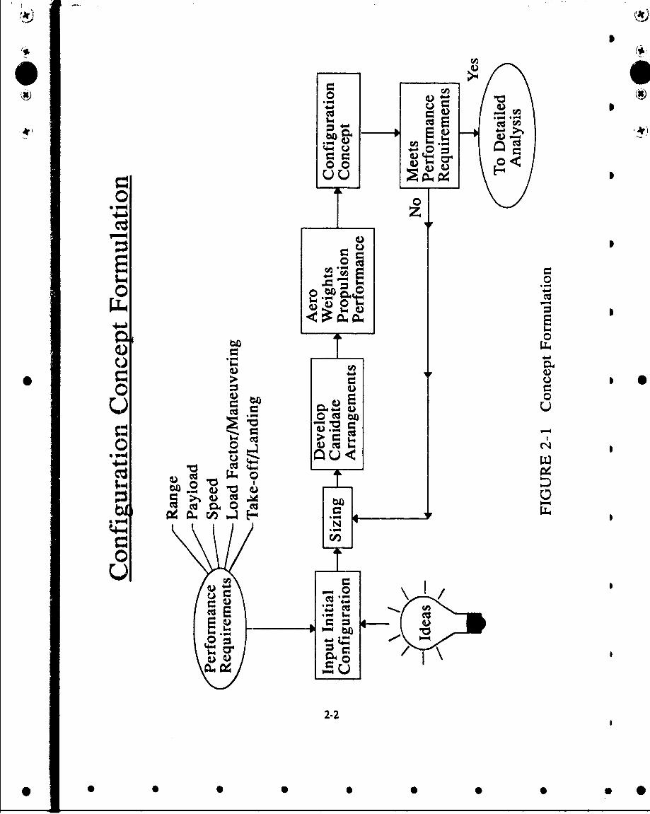
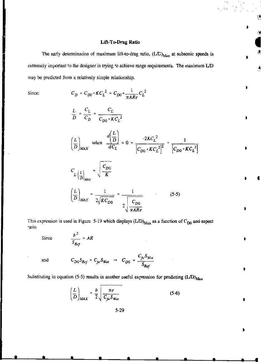
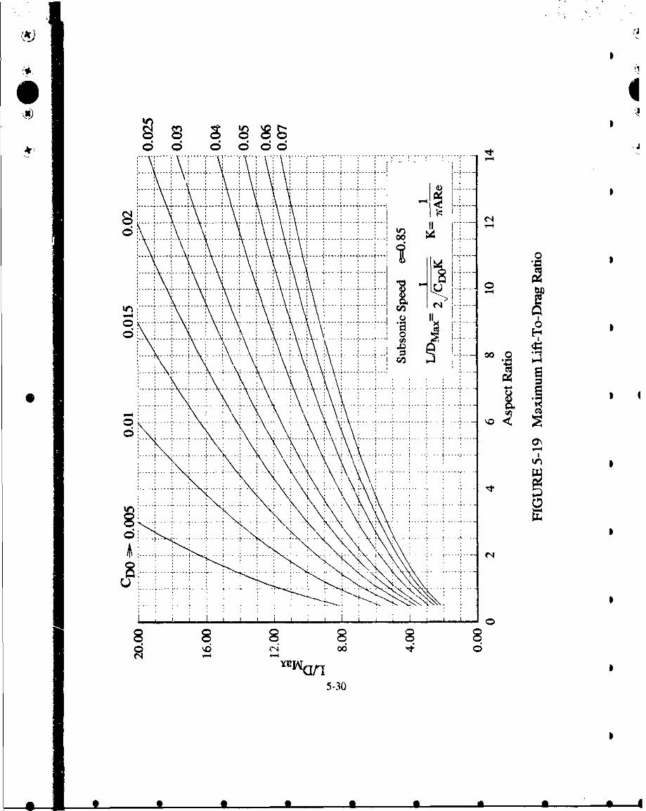
4,) The range of an aircraft is a critical performance parameter and it strongly influences the
wing design. The primary aerodynamic parameter which drives the configuration is maximum
lift-to-drag ratio, (L/D)Ma. The lift coefficient for (L/D)Max is called the optimum CL and is
given by: CL O (6-1)
and the required CL for one g level cruise flight is:
CL J•e = .W162q Sj~ (6-2
then for CLRe=CL Opt - Cq - (6-3)
0 Therefore, at maximum LiD, airplanes fly at an altitude and velocity to satisfy equation (6-2).
Hence for a fixed velocity and wing loading, the cruise altitude is defined for maximum L)D.
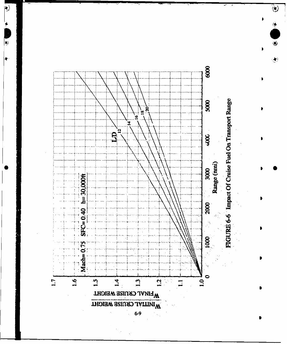
Historical data is pmsented in Figure 6-5 to evaluate cruise altitude based on take-"ff wing
loading. The data indicates cruise altitu.c dmcrAscs as wing loadi-g increases, but begins to
level off at wing loadings above M6Wpsf. The crtise raang of an aircraft can be estimated 4 uitc
accumately by the imguit range equation gin• beltw:
R V v~, 1.[Jg ,i64
with R in tautic-al milesV in k"sSRK' in lbs of fuel p-r bwor per pound of thrust11) lift to drag ratioWIAFVp initial cruiuc weightlfinal cmiu.i weight
6-6
116
:.•+ • ..: .• .• ..:• .•.. .- ... ...... ...•.• .• . • -. - •• • • - ... :........:
:.. •.. •.. ... ... ..•.. ... ... .. ...• ... .• ..• ..• .•. .•... ... ... .. . ..•. ...... •........... ... o...
!.. ..' - ..•...i.. ±...I. ... L.............-...:................-.L...-.... .. •.-. ...- . .. . .. ...-... -
II
S. . . . .: , , : : : : , ,•, : : •,• : ...... ,...... :
S.............~~ ~~............ ........... . . . : . . . . .: , , , . ... .: .. ...... . . . ... ........ ...:. _
............. ... .. * .. [... ..... ... ...•, . . , •...:, .L . .,.'. .. .. . ..... .. . ... -... ... . -
S.. ..: • :,: : : ! ! i i ! ! • , ! ! ! ! , i i i'L : '-*... ..,, ... .. ........ ......... .............. J
-. :, o .- . .. ... -" •,€ : "• •• : -....... ..!• "r -..' : - - "• "
6-7
-1 -
Assumptions used in developing this equation include cruising at constant (LID) (go constant
altitude), constant velocity and constant SFC. Thus an increase in I/D, a reduction in SFC, and
an increase in fuel fraction will lead to increased range.
The impact of lift-to-drag ratio on cruise range for transports is shown in Figure 6-6. Since
fuel fraction for transports (Figure 4-7) varies between 35 and 45 percent of the gross take-off-
weight, and typical cruise fuel loads account for 45 to 55 percent of the total fuel load, a
representative range of values for cruise fuel weight to gross take-off weight is 0.15 to 0.25.
Hence, a transport with an L/D = 16, an initial cruise weight to final cruise weight ratio of 1.25
would have a nominal range of 3800 nautical miles. A similar chart for fighters is presented in
Figure 6-7. Since the nominal fuel fraction for fighters is 27 percent of gross take-off weight
and typic.al internal cruise fuel loads are about 30 to 40 percent of the total fuel load, a nominal
range of values for initial cruise fuel weight to gross take-off weight is 0.075 to 0. C25.
Therefore, a fighter with an LID = 10, an initial cruise weight to final ciuiaz weight ratio of 1.10,
would have a nowinal range of 500 nautical miles.
The impact of supersonic speed to fighter range is mradiiy appawvnt in Figore 6-8. Assuming
an UD = 4, at an altitude of 40.000ft, SFC= 2.0 and an initial to final cruise weight ratio of 1.10.
the fighter range is only 225 naiutical miles. This is over a 55 percent reduction in range
capability. "Tis is optimistic since large quantities oil fuel will be coLsumed during •ickleratio
from Maclh 0.9 to 2.0. 11T acceleratioi fuel will d&x sc' the fuel avaiiablu for cruise tligjht.
Thus there is a significant penalty for superonic speeds. hiWs large Xmealty may be reduced
thmugh the use of very high fuse•a•e fiteviss ratios, ima" wing swcepback anzlgi aswd situal
wing thiclatess ratios.
6-8
m • = = • • m • w • • • • = •
- - - - - - - - -. . .. . . . . . . .. .. . .. . . .. . .
.... .... ... .. L... .. ..... ... .... ...
-- -- -- --- - 4 . . .... . .. ... .... . ..
.. ...... .. .. . .. .. ......
*.................... -. ------
-0- .............. ......-- -
tft
0 .&'Sl-d: ' 4 - -MOW&RS-lo VUIAAI
6-93
0
.... .- - A- .A- ....L...- L- - - - - - -..
. . . .....-- - - -- --- --- -
.. .. .. ... .. . . ..-- -- ---. . .
- - - - - - - - - -- - - - - - - - - - - - - - - - - --.. . . . .
*rZ
.......... .-------------------.
*ý It
.1 Hla A~i.......-LOM H- l - .MA0
~6-1
------------...... . ...... .......
---- ---...... -- - ....
................... ................
......... ........ .... .... ...S. . ...................................... r...
........................V...................................................... .......
..... .. .. ...... . . . ... ..I
.. . . .. . . .. . . . . . . . . . . . . . .. . . . .
. . . .. . .. ..
..........
t~q.4
jL~oamaintiv~AX_
Much attention in the 1970's and 80's was given to investigating the technologies which
3maximize the range parameter M(LID) (References 29-32). A class of vehicles calledSFC
"Osupercruisers" were envisioned where LID at higher Mach numbers was maximized while
keeping engine throttle setting below afterburner for low SFC. This was a severe challenge to
the aerodynamicist in trying to maximize supersonic LID and maintain acceptable transonic
maneuvering characteristics. The design options for increasing high speed LID impact the
available fuel fraction, while the thrust required at non-afterburner engine power settings defines
engine size, which in turn impacts vehicle size, shape, weight, fuel fraction and LID. These are
the conflicts which must be resolved early in the design cycle.
In order to permit rapid estimates involving aircraft range the following approach can be
used. If a cruise range segment is divided by the fuel consumed for the distance traveled a
parameter called specific range is formed, with units of nautical miles per pound of fuel. This
is an average value of how far a particular aircraft can travel on one pound of fuel. The
instantaneous specific range is found by dividing the flight velocity by the fuel flow
SR V V (6-5)FF
where: V - nautical titles pet hourFF - lbs of fuel per hourSR - nautical miles pcr lb of fuel
Equation (6-5) may be expessed as
SR V VsR ~3- s''FY~ SFC X 7'
Wand for T=D; L=W; and D -
6-12
O I ... O t • •• •
SFC x W
For a modem aircraft at Mach 0.9 and 30,000 feet: 4
LID= 10,SF.C = 1.0 lbsihrllbV = 516 knotsWI = 25,000 lbs
SR-- (516)(10)
t el 1.0(25,000) m= 0.206 nm.•
1b
Another often used parameter is the range parameter which is composed of parameters fromS
the Breguet range equation.
RF =PSFC * 0
It is often used to compare aircraft capabilit-y based on aerodynamics and propulsion efficiencies.
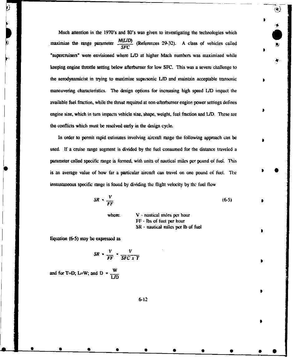
A rapid approximation for the fuel required for a cruise mission segment can be made by
dividing the range required by the specific range. S
SPECIFIC EXCESS POWERIMUNEUVERING
Sptifit cx cess power is defined asS
Ps -I" r- D(6-8)
and is expimseA in the units of fw- per setond. Simple aircraft forc equilibrium shows thlt Ps
is the rate of climb an aicratq can achieve under the approximations of shallow climb angles and
,m,acwxrcmted flight (Retcraces 33 io 35). However as cureutly us- Ps is betea
6-13
0S 0 0
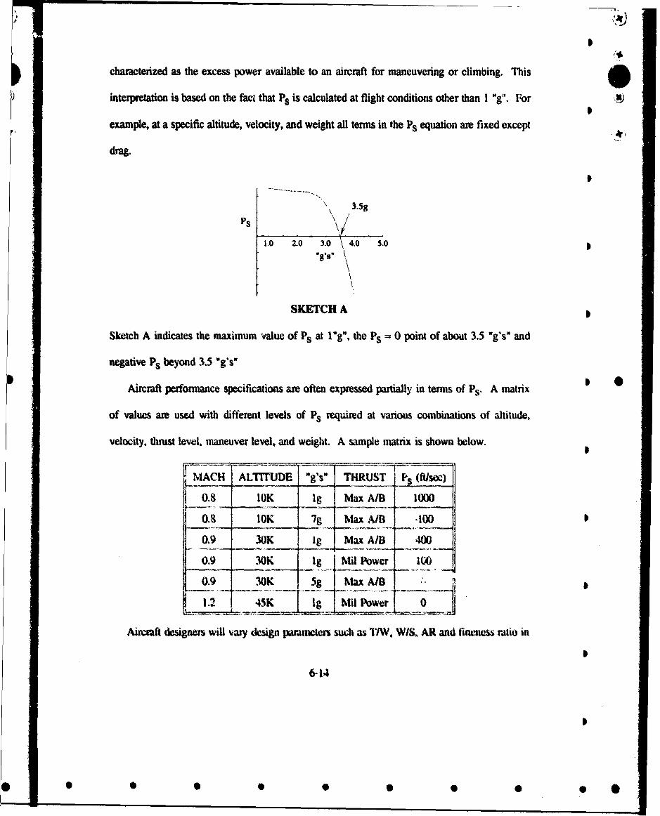
characterized as the excess power available to an aircraft for maneuvering or climbing. This
interpretation is based on the fact that PS is calculated at flight conditions other than I "g". For ,3Im
example, at a specific altitude, velocity, and weight all terms in the PS equation are fixed except
drag.
Ps
3.5g
1.0 2.0 3.0 4.0 5.0"g's" \
SKETCH A
Sketch A indicates the maximum value of PS at I *g", the PS 0 point of about 3.5 "g's" and
negative PS beyond 3.5 "g's"
Aircraft perfonrance specifications are often expressed partially in terms of Ps. A matrix 0
of values are used with different levels of PS required at various combinations of altitude,
velocity, thrust level, maneuver level, and weight. A sample matrix is shown below.
MACH ALTITUDE "g's" THRUST PS (ft/sec)
1 0.8 0K Ig Max A/B 1000
0.8 10K 7 Max AIB 100
0.9 30K I Max A/B 400
0.9 30K Ig LMil Power 106
0.9 INK 5g _Max A/8
Aer -aft designers will vary iksagn pamimetei such as T1W. WIS. AR and finemws ratio in
6[ 6-14
• • • •• • •
0 6 0 S~~ S 000
an attempt to meet these perfornance requirements (as well as others). Often meeting one
particular requirement such as the 5g, M=0.9, h=30,O00 ft. point in the example above will ensure
that the other requirements are also met.
Contour plots of Ps against altitude and Mach number are often generated to show the global
perfonnance capability of an aircraft. A typical example is shown in Figure 6-9. The Ps = 0
lines indicate on a "lg" chart the flight envelope capability of the vehicle. On charts for
conditions above I "g" (Figure 6-10) the PS = 0 line indicates for each Mach number the
maximum altitude at which the aircraft can sustain the "g" level of the figure.
Another valuable use of the PS performance parameter is in comparing one aircraft against
another. This is typically done in evaluating various aircraft design solutions and in evaluating
the performance advantages and disadvantages of threat aircraft. An advantage of 100 feet per
second is generally accepted as significant when comparing aircraft performance, * *SUSTAINED MANEUVERING
Another classic performance parameter utilized is maximum sustained "g" capability. As
indicated in the previous discussion PS and maximum *g" capability are closely related. When
P. is equal to zero an aircraft is at its maximum sustained "g" level with thrust equal to drag at
the t•ueuver level. This "g" level can be detenmined as follow:
When PS= 0;WheuP -- P -)
w ~iV
qS
6-15
• • • •• • •
solving for n results in the following relationship
,a;
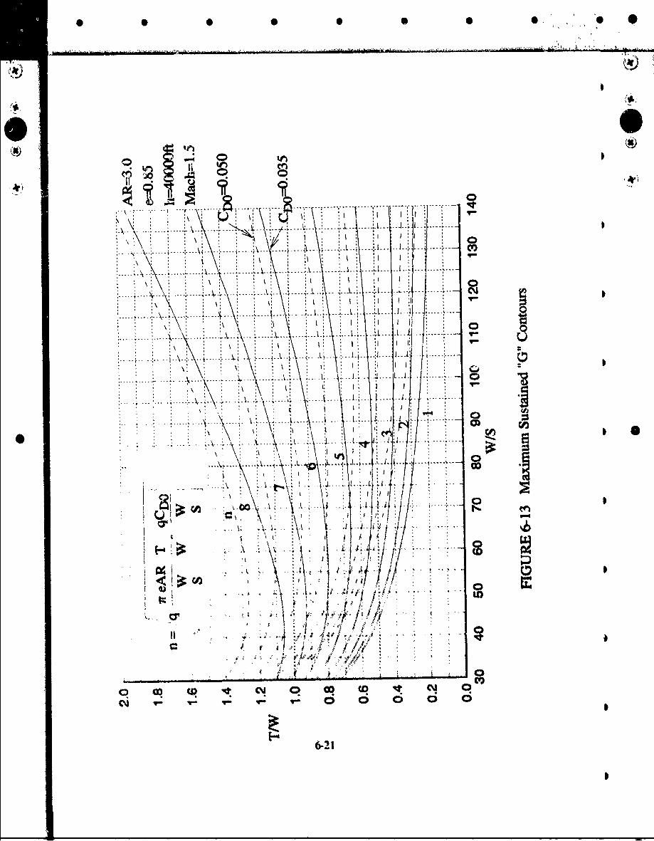
n = q7t'AR T_ qC-9)WI iV W4
Figures 6-11 to 6-13 have plotted this equation in paiametric form for values of AR. "W, and
CD0 typical of modem aircraft. one interesting interpretation of Figure 6-12 is to note the
variation of required T/W as WIS varies while keeping the maneuver capability constant. This
type of chart ,aa identify design choices for meeting maneuver specifications with either fixed
or "rubber" engines. Note in Figure 6-12 that the effect of CDO on the required T/W at a
constant WIS is relatively small for this condition. The effects of wing planfonn (AR) and
design technology ("e') can also be estimated with equation (6-9). Figure 6-13 indicates similar
data for supersonic flight conditions and typical tighter aircraft parameters.
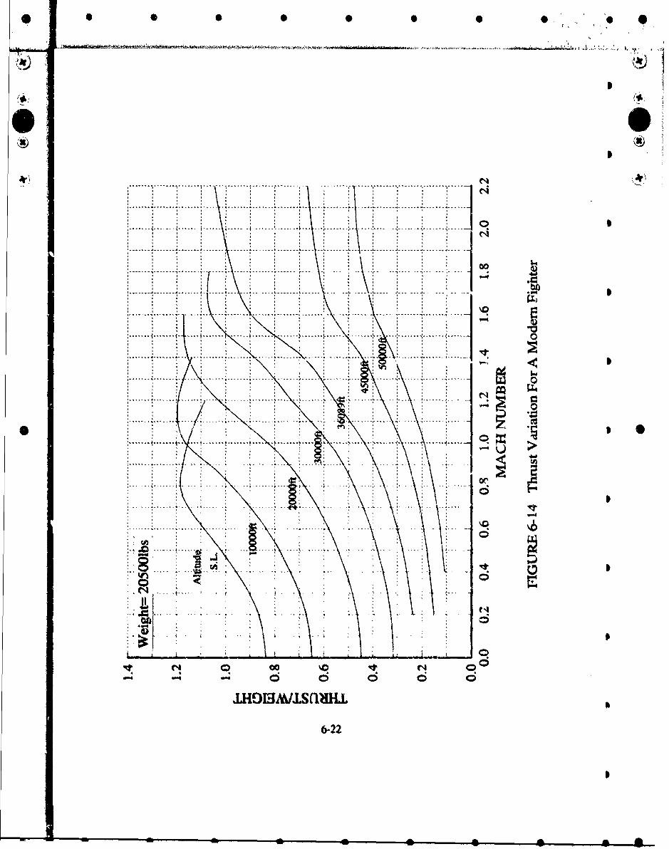
In using equation (6-9) it is important to note that the thrust-to-weight. T/W, parameter is v *specified at the particular flight conditions under consideration. Thrust-to-weight and wing
loading, WIS. are often used to characterize the performance levels and design emphasis ofI
aircraft, high TIW and low WiS representing high performance. Since thmst varies with altitude
and Mach number and wing loading varies with payload and fuel consumption; thrust to weight
values are usually quoted at some refrnce condition such as sea level statiic maximum thrust
and take-off gross weight. Figure 6-14 pa.sents the varia-Jon of T(%V for a typical modeni fighter
with both M1ch number and altitude, Cwunt high pefrtfon1ainue ilghtcs have TAV valus around
1.0 or greater at sea level rfkemwo conditions aid decrcaue to I1 these valutm at mid altitude
and transonic speo.
In awssing the tlatrionships bctween pctfrnwmau, veuitenwn•ts, iypitally 11S Aund .susaintdlp
.6-1g
S 5 0 • 0 0 0 0 •
* .7... . ........ \.. .. .. -- - --- -- - .. ..... . . . .. .. .
-..........
.... .. .* ... 0 ---
......... ........ c. .... ...*. ....... .
.........
V4 -
6-20
0 0*
*99
........... .. .......... .\......... ............ .. ....
A . .... .... -k c~... .... . I I
.t ... ... ....
.... ..... ..... .....
\\. ....\ . 0
iv~
0~~~~~ 43 V( OtC
6it21
.. ..... .... ... .. ...... .. ...... . .. .. .. 0. . ....... .... .. ..
* ............ ... ...
S.......... 4 .. . ...
S. . ....... .... 4........ . ..... -------- 0.....
.......... ......................... .............-----... ..............
.. .... ........ .
S.... ............ ............. ... . . . .
ell
"a. 00
- 0 6 o 6a~dH
0 0 0• 0 0 .0, 0' 0 0
g's, on aircraft design drivers such as T/W, the following observations provide some guidance.
Using the PS equation (6-8) results in
T [ D]
T - If D=O
T Psor For D > 0W V
Given a PS specification at some altitude and Mach number we can immediately establish a lower
bound on T/W at those conditions. To obtain a better estimate consider
D I If L= W
if we return to the Ps relationship we have
T Ps 1
L L
The minimum value of 1 resultswhen L D (irsl t -DDD j
T Ps Iso - +. •
At mnueuver lift coefficients where L- nW, (L/D)t.tNa, is less than (I/D)Mr so the final
estimate is
6-23
a • •• • • •• •
0 0 0 0 0 0 0 0 0 0
T r> OS
)Mau
A typical value for L/D at high speed, subsonic maneuver conditions for current fighters is 3 to
4.
The T/W's estimated by the above procedure can be scaled back to reference conditions
using propulsion data from a candidate engine (see Figure 6-14 for trends) or the following
approximation when data is not available.
TATFPJDE =TSpA LEVl - I
TURN RATE
Another performance parameter often used is turn rate expressed in degrees per second and
indicates how fast the pilot can "point the nose". Turn rate for sustained maneuvering is simply *
related to the g capability of the aircraft through the following well-known expression
V
Figures 6-15 and 6-16 present parametric data for quickly converting between sustained maneuver
and turn rate.
All of the expressions used or developed in this section relate to sustained maneuvering
which is an idealized steady state condition. Instantaneous maneuvering is also used as a
performance requirement and represents a more dynamic condition. Instantaneous turn rate or
maneuver level is typically characterized by maneuvers at CL &tAX or a structural limit for limited
durations and drag levels above available thrust. These maneuvers result in negative Ps and large
6-24
• • •I • • •• •
* u 0 S Si i 0 0 0 w 00
it)~
SI-.-.b . ...........--- ------
00 00
.. . ... .. .
~. , .......
------------------------------------------ --------------------------------------------
.. .. . ... .. . .. . . . . .
...................................................
.......--.....--.....,ksSe)a. jj
6-25S
I - -- -
- , , , --
*- ..... ~ .. ........ .. ....~ .I.....
---- ----- -I.t-- -- -- -
. . . . . ..5 .......................... . . . . . . . . . .---
.............. ) S....... ----- 4........I. S .
............. ~ ~ ~ ~ ~ ~ ~~~~~~~~~ .... .. . .. ... .......................................
.S .......... ...... . ...... ..... L ...... S .......... A S.
~~~~~~. .........4. .. I.....~.. .
......... ............... v ~ .
0 ... ...... ............ .................
...... ............ .......... L....... ...... ...../
.........................
6-26
changes in velocity and/or altitude, hence the name instantaneous as opposed to sustained.
LANDING
Landing performance is primarily dependent on tile approach speed and the deceleration
generated from braking (ignoring reverse thrust). The approach speed is normally defined as
20% above the stall velocity for CL MAX, which can be determined from Figure 6-1. A good
breaking system can provide a mean deceleration rate (-a) of -6 ft/sec2. Figure 6-17 provides the
landing ground distance as a function of approach speed and deceleration and is based on the
relationship:2
Distance = App-2a
Landing distance calculations normally include the horizontal distance traveled during the descent
from a standard 50 foot obstacle. Figure 6-18 presents this air distance as a function of descent
angle or glide slope y, which is defined as the angle whose tangent is the ratio of vertical
distance to horizontal distance and is also represented by the reciprocal of the lift to drag ratio,
including power, in the approach configuration (L(D Power Approach), flaps and landing gear
down, and also approximlates the resulting thrust to weight ratio [-D-
6-27
• • •• • • •• •
0 0 ... . . .. . 0,0 0
*
+ • :• -• T -.......... ...... r ....,,: ".... ,".... r.... ".... r..... r .• .-•-C i.• --',....+ ... , ....•.. -_ .... •.... •...... ..... •.... •. mi -... .. . . .. .... ....I. I
',• .... --}-\ - . ........ ... , ..... - i -.... :.... ,.... •..... , III • -: ........ " ... +-.• ... .......... • ............ ......Il I l il ..
-' " .... ..... - -- - - -.... . .", '• .. . . .". .. ; . .;-/I ------- 9---- ....... ......... .....
,•f, .... • • ?"• '-i ..... : ... !.... !....... ;• l• • - l
S ... .. ...... ......
. ---- .... h- --- - .. --- .----.... .......
i •. , _ . ,' . • ' . ..: .x _.• i .. . .. .• .• _ . .. .......... .........••• :..x ....• ....• ....."............iLm •.. . • ......... . .-.-.. i- i. L .. ,... <•
:iiii~~~~~~~~ilil-.~~~~~~ .........l~l .. IIIII:II:II:IIIIZ I21111.................. .... ..... .... .... ... ..... ., . . ,. . ,. . .:....... .. .,... .. ... ...... ..,,..... .. .. ........ ... .... ,. . . .+. . . .•. .-----------------.. ---- v- ... ! s... i- ..i.. --- --------- -- •.. ..•..
(sx) HOVOUddVA
6-28
• • •• • • •• •I
4---- f-4-I T - r-*
11 --- T - 1....i
........ 0 0
......... . ......
N~ 00
gap - A ajaiy OdOIS aP!ID
6&29
7. PROCEDURES FOR THE FORMULATION AND ANALYSIS OF ANAIRCRAFT CONFIGURATION
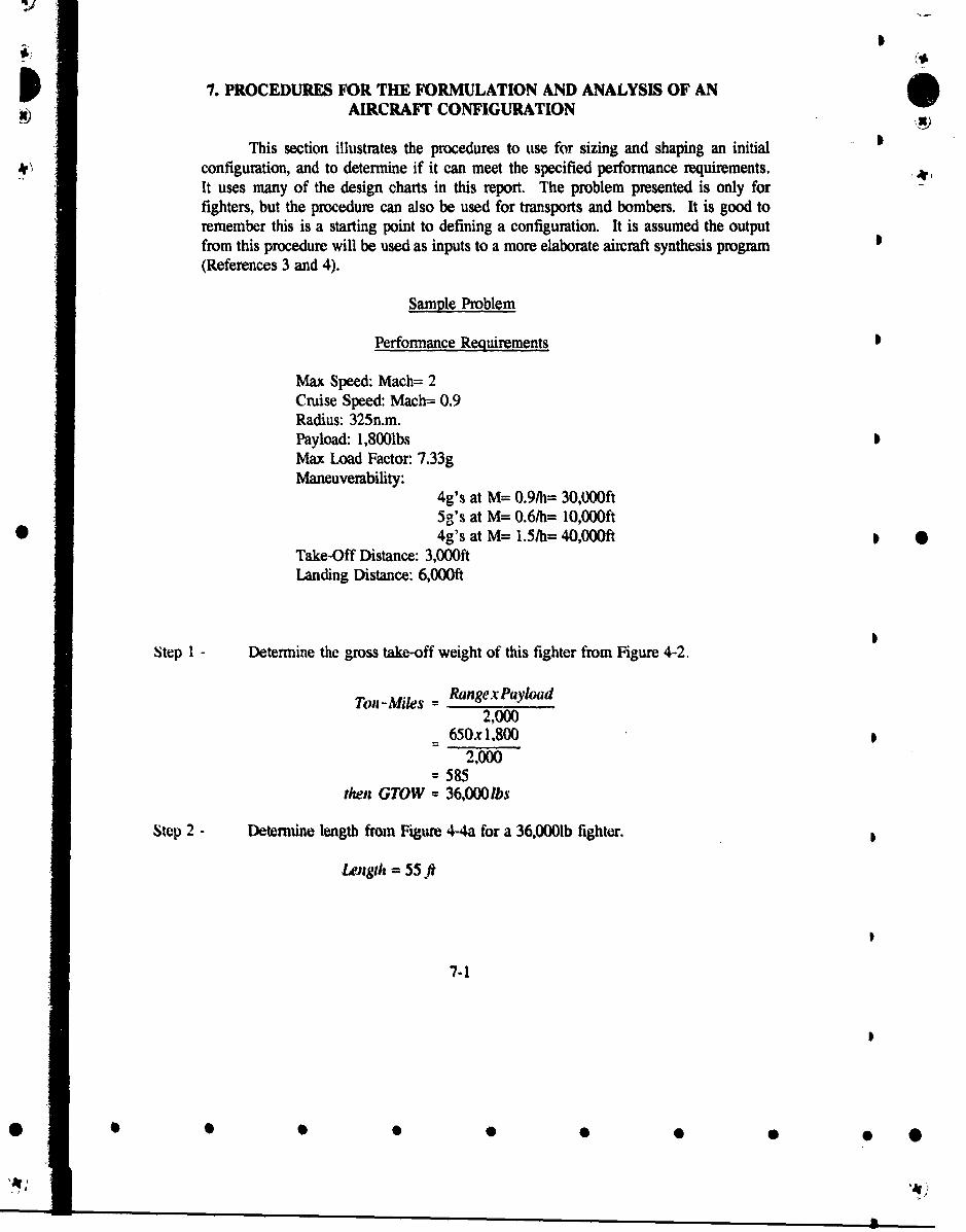
This section illustrates the procedures to use for sizing and shaping an initialconfiguration, and to determine if it can meet the specified performance requirements.It uses many of the design charts in this report. The problem presented is only forfighters, but the procedure can also be used for transports and bombers. It is good toremember this is a starting point to defining a configuration. It is assumed the outputfrom this procedure will be used as inputs to a more elaborate aircraft synthesis program(References 3 and 4).
Sample Problem
Performance Requirements
Max Speed: Mach= 2Cruise Speed: Mach= 0.9Radius: 325n.m.Payload: 1,8001bsMax Load Factor. 7.33gManeuverability:
4g's at M= 0.9/h= 30,00Oft5g's at M= 0.6/h= l0,O00ft
* , 4g's at M= 1.51h= 40,000ft * 0Take-Off Distance: 3,000ftLanding Distance: 6,000ft
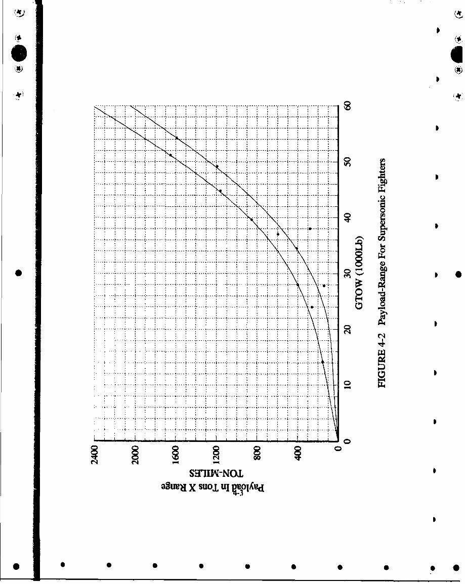
Step I - Determine the gross take-off weight of this fighter from Figure 4-2.
Ton -Miles = RangexPayload2,000
650x 1,800
2,000= 585
then GTOW 36,000lbs
Step 2 - Detemine length from Figure 4-4a for a 36,0001b fighter.
Lengh = 55 ft
7-1
* S••• •0 0
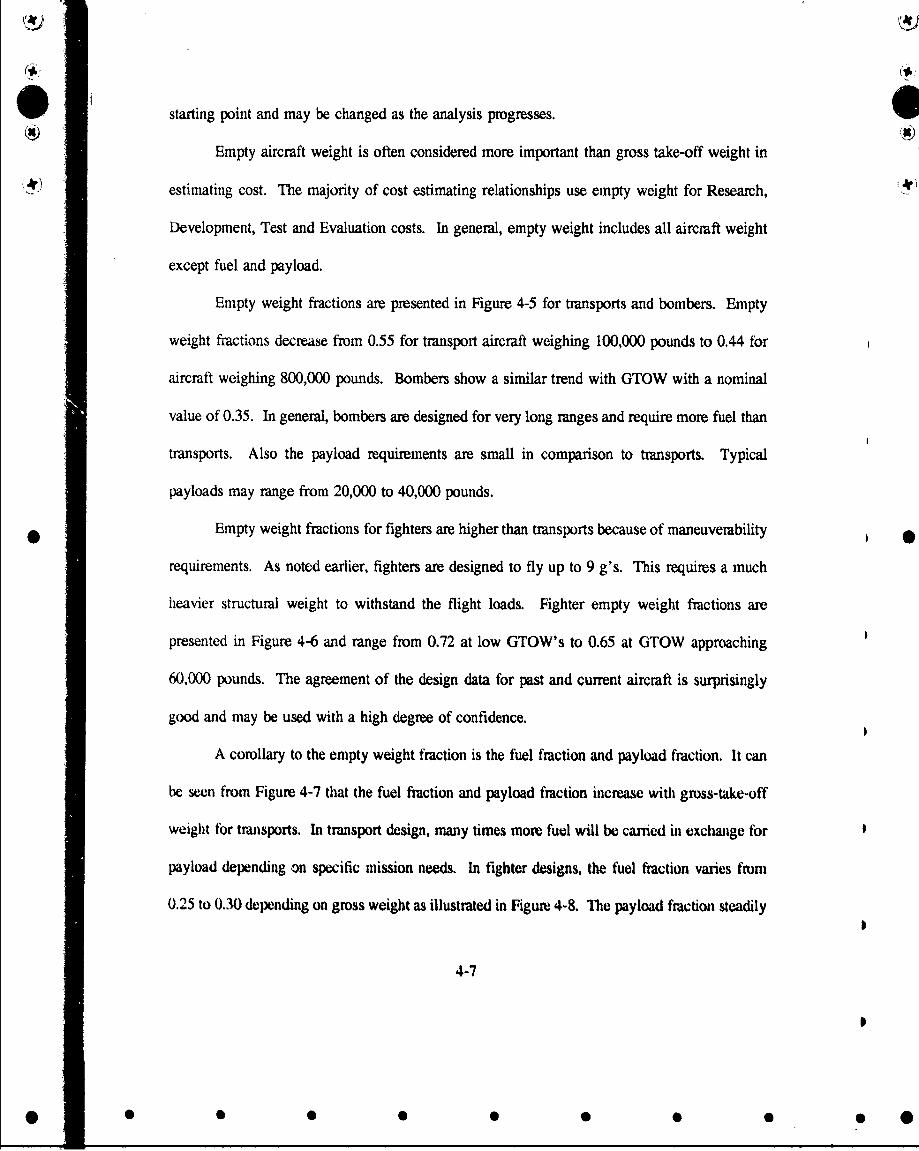
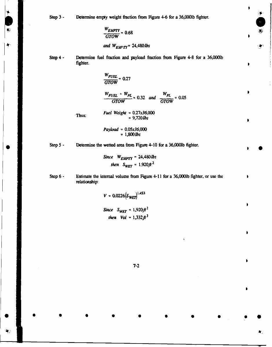
Step 3 - Determine empty weight frction from Figure 4-6 for a 36,O0Olb fighter.
WEMPTY 0.68
GTOW
4V and WEMrl,- 24,480/bs 4'
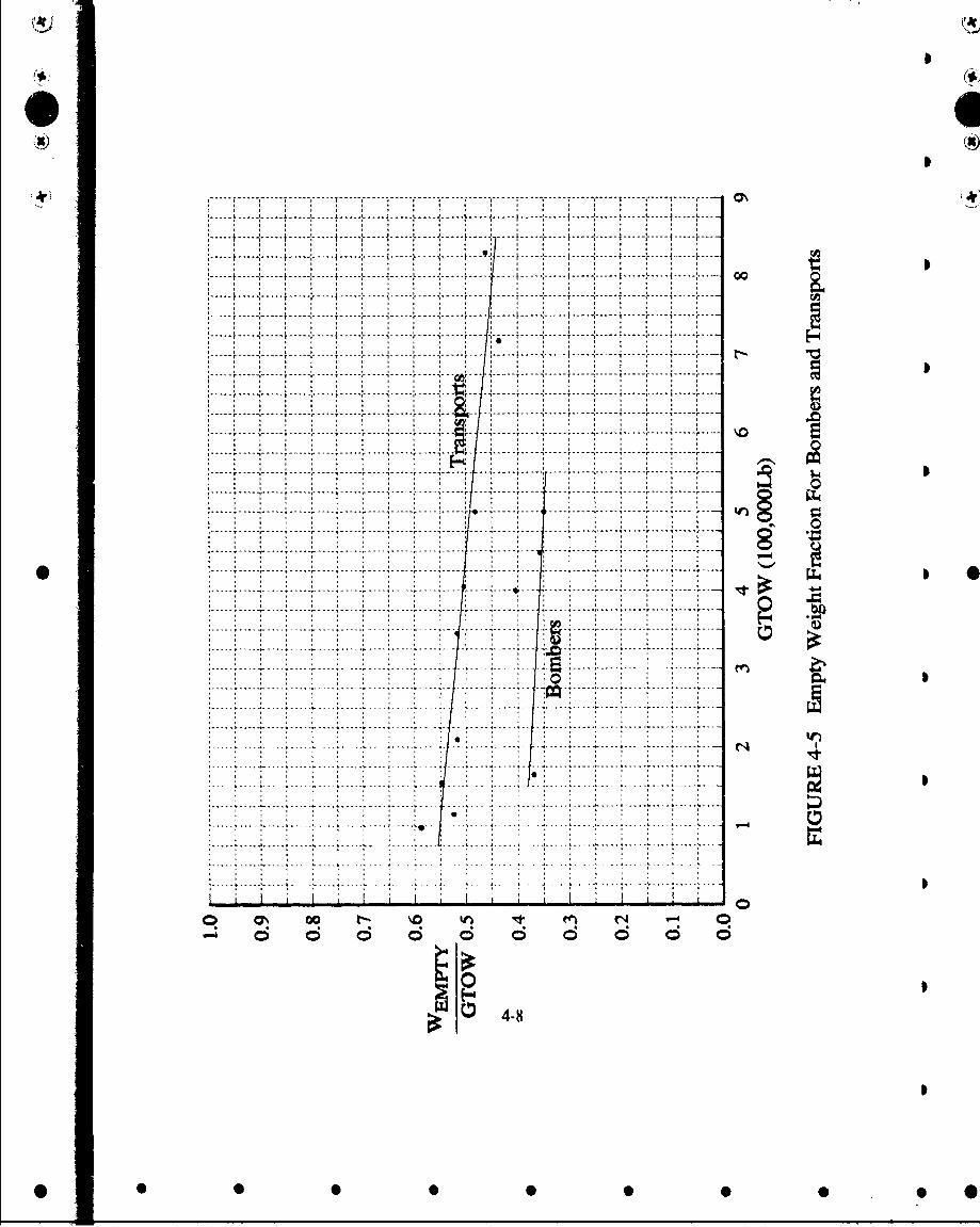
Step 4 - Determine fuel fraction and payload fiaction from Figure 4-8 for a 36,0001bfighter.
WFUEL .0.7
GTOW
WFUEL + WPL = 0.32 and WpL f 0.05GTOW GTOW
Thus: Fuel Weight = 0.27x36,000= 9,720lbs
Payload = 0.05x36,000
= 1,800 lbs
* Step 5 - Determine the wetted area from Figure 4-10 for a 36,0001b fighter. *
Since WEMp,- = 24,480lbs
then SW -= 1.920ft2
Step 6 - Estimate the internal volume from Figure 4-11 for a 36,0001b fighter, or use therelationship:
V 0.0226(SWE•"43
Since SWT. = 1,920fi2
then Vol - 1,332fl3
7-2
'Aý • •
"*r 0 SSSS
• • w #
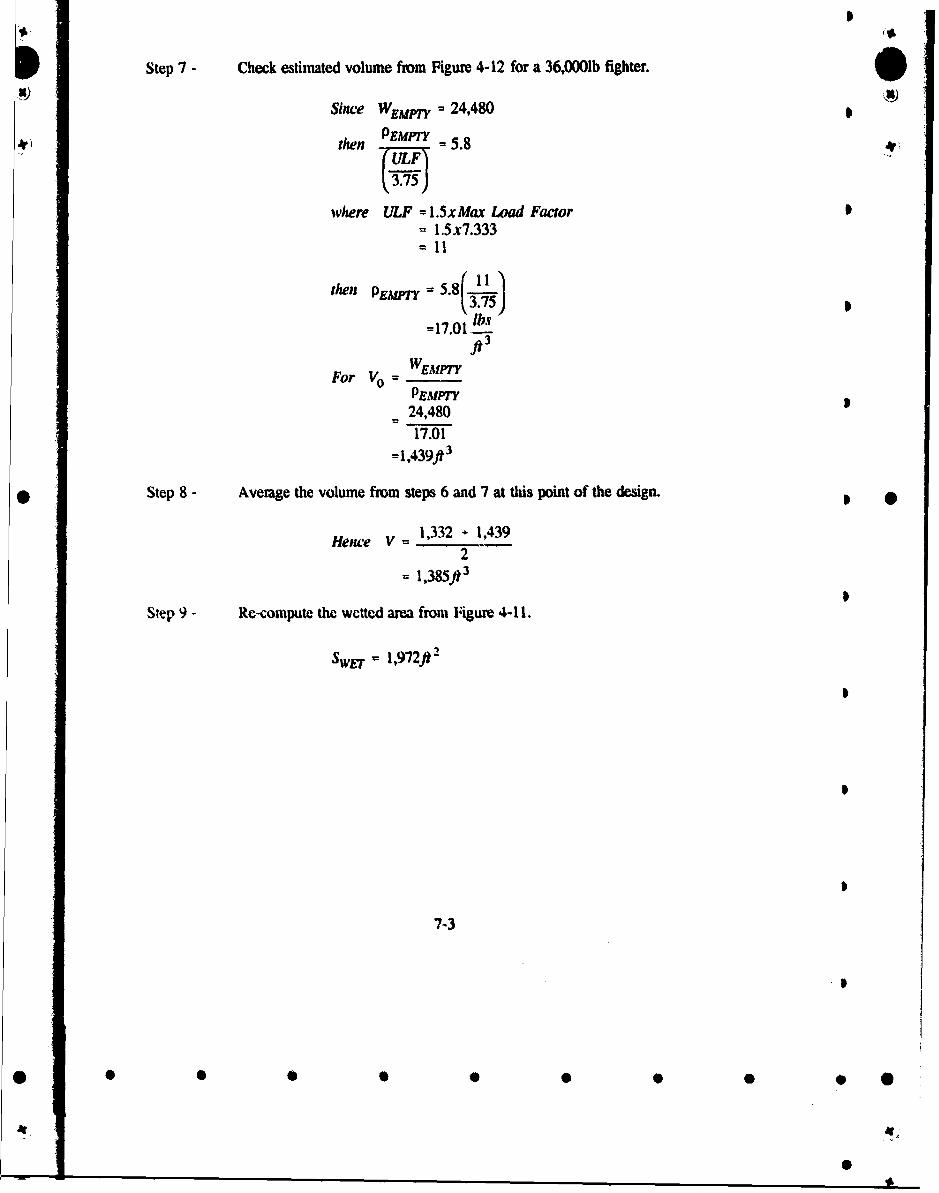
Step 7 - Check estimated volume from Figure 4-12 for a 36,0001b fighter.
Since WMp, = 24,480
t hen PEMPT" = 5.8
where ULF =-1.5xMax Load Factor= 1.5x7.333
11
then pE pn~q 5.8 (k11thn1%un ,3.75) 5
=17.01. lbsft3
For V 0 =WEMPTY
PEMPrY
24,48017.01
=1 ,439ft3
* Step 8- Average the volume frm steps 6 and 7 at this point of the design. *Hence V = 1,332 - 1,439
2= 1,385ft3
Step 9 - Re-compute the wetted area from Figure 4-11.
Swu = 1,972fJ
S!
7-3
A .•
* 0 00 0 S 00 0O
• tiiim • 0 i
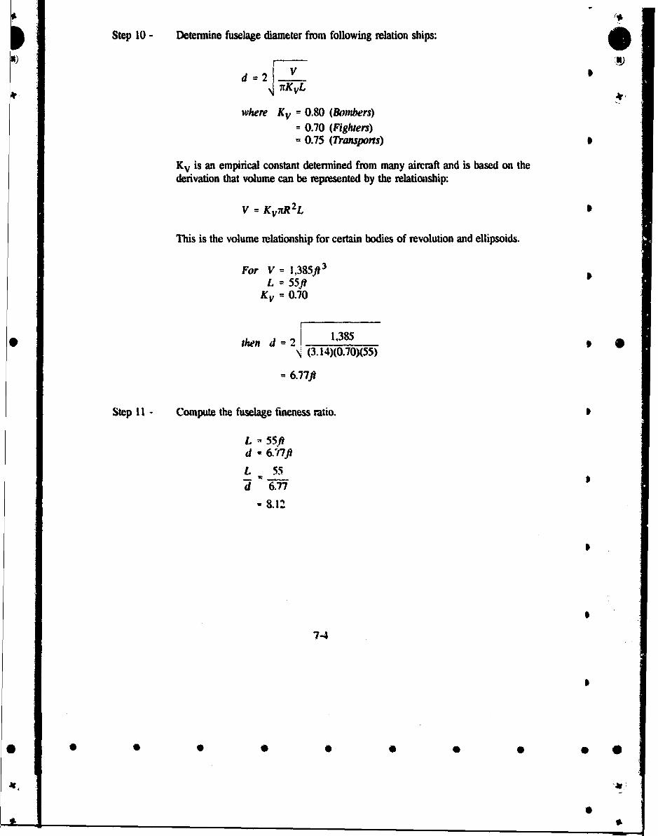
Step 10 - Determine fuselage diameter from following relation ships:
d-=2 V7IKvL
where Kv - 0.80 (Bombers)= 0.70 (Fighters)S0.75 (Transpons)
Kv is an empirical constant determined from many aircraft and is based on thederivation that volume can be represented by the relationship:
V = Kv7,R 2 L
This is the volume relationship for certain bodies of revolution and ellipsoids.
For V = l,385ft3
L = 55ftKv = 0.70
I
then d = 2 1 1,385S(3.14)(0.70)(55)
= 6.77ft
Step 11 - Compute the fuselage fineness ratio.
L - 55.f
d -67-7fl
L 55d 6.77
II
7-4
AI
* S SS *
• • • •• • •
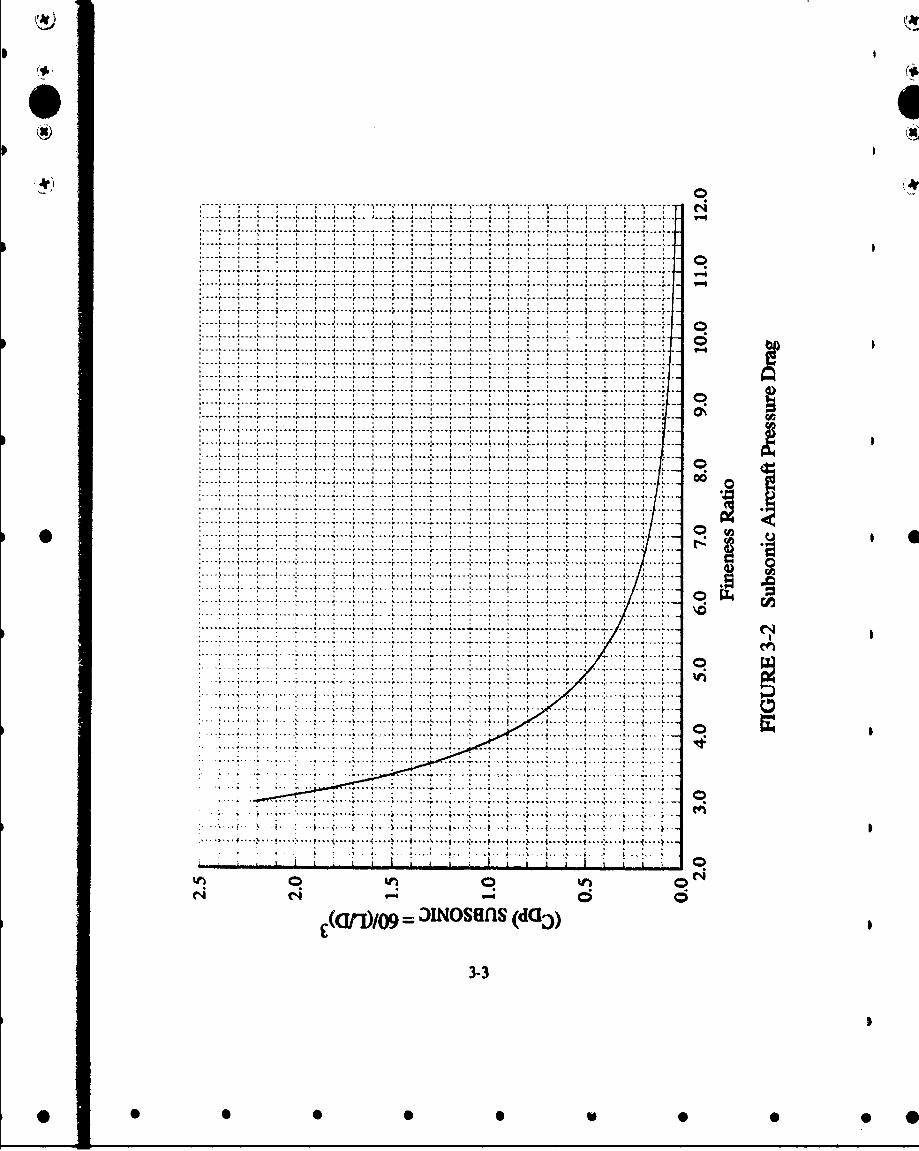
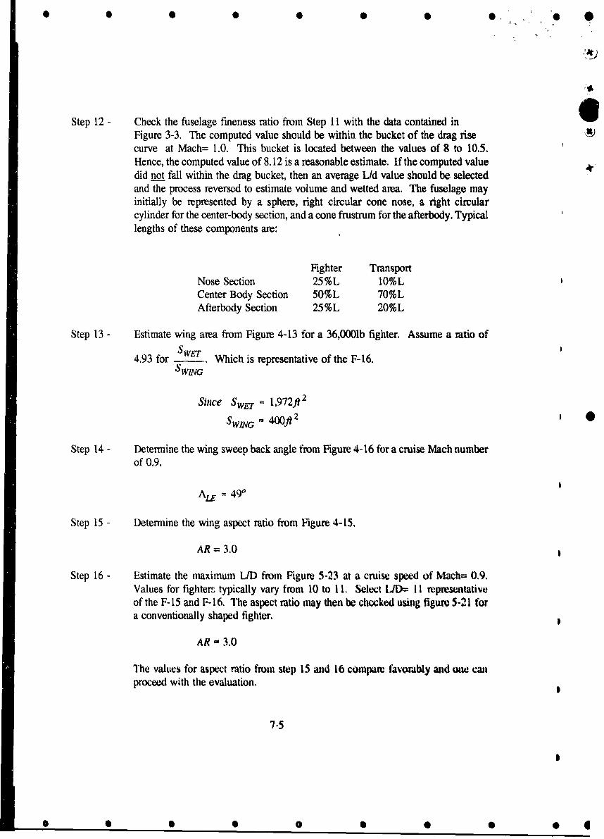
Step 12 - Check the fuselage fineness ratio from Step 11 with the data contained inFigure 3-3. The computed value should be within the bucket of the drag risecurve at Mach= 1.0. This bucket is located between the values of 8 to 10.5.Hence, the computed value of 8.12 is a reasonable estimate. If the computed valuedid not fall within the drag bucket, then an average Lid value should be selectedand the process reversed to estimate volume and wetted area. The fuselage mayinitially be represented by a sphere, right circular cone nose, a right circularcylinder for the center-body section, and a cone frustrum for the afterbody. Typicallengths of these components are:
Fighter TransportNose Section 25%L 10%LCenter Body Section 50%L 70%LAfterbody Section 25%L 20%L
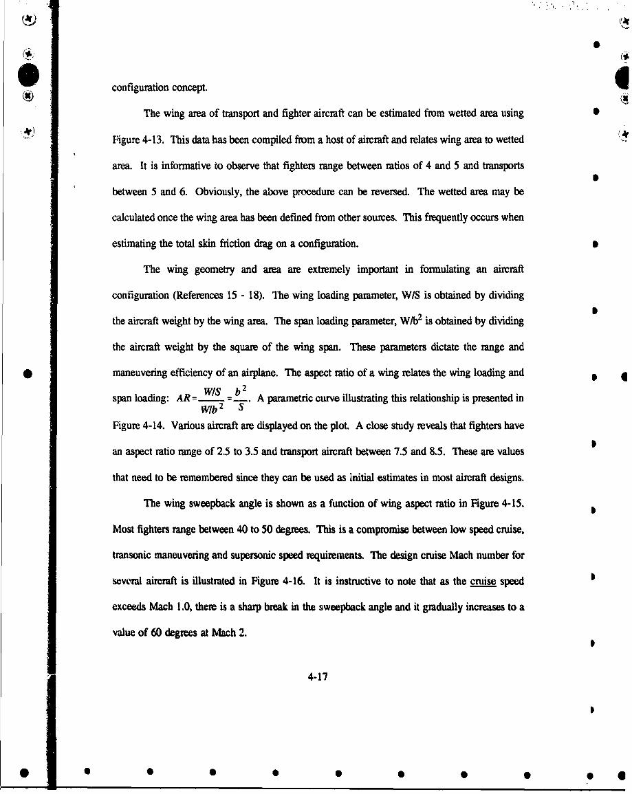
Step 13 - Estimate wing area from Figure 4-13 for a 36,0001b fighter. Assume a ratio ofSWET
4.93 for _ . Which is representative of the F-16.SwSWING
Since SwET = 1,972ft2
SWING - 400ft 2 *
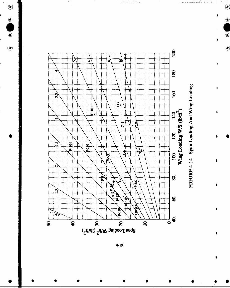
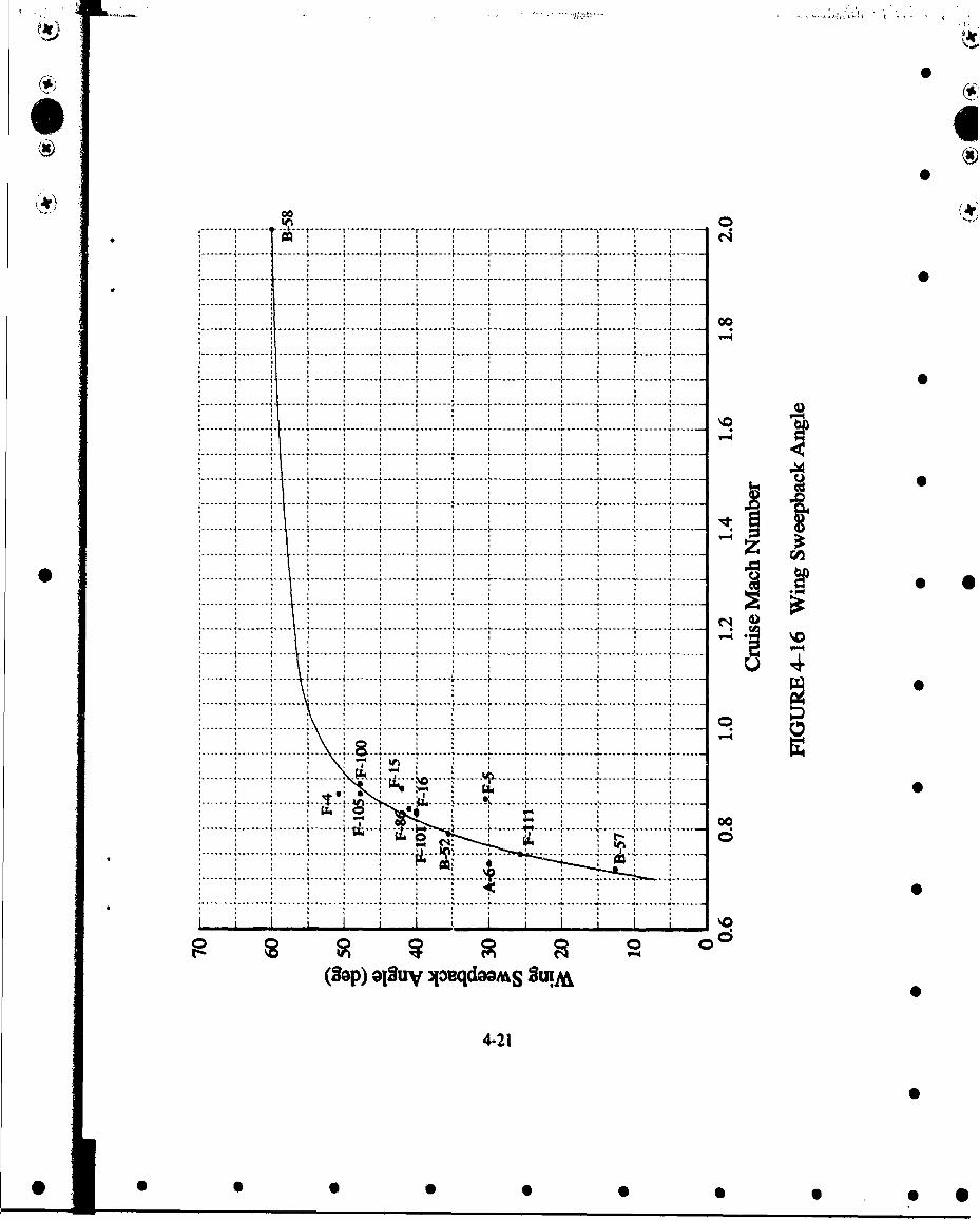
Step 14 - Determine the wing sweep back angle from Figure 4-16 for a cruise Mach numberof 0.9.
ALE - 490
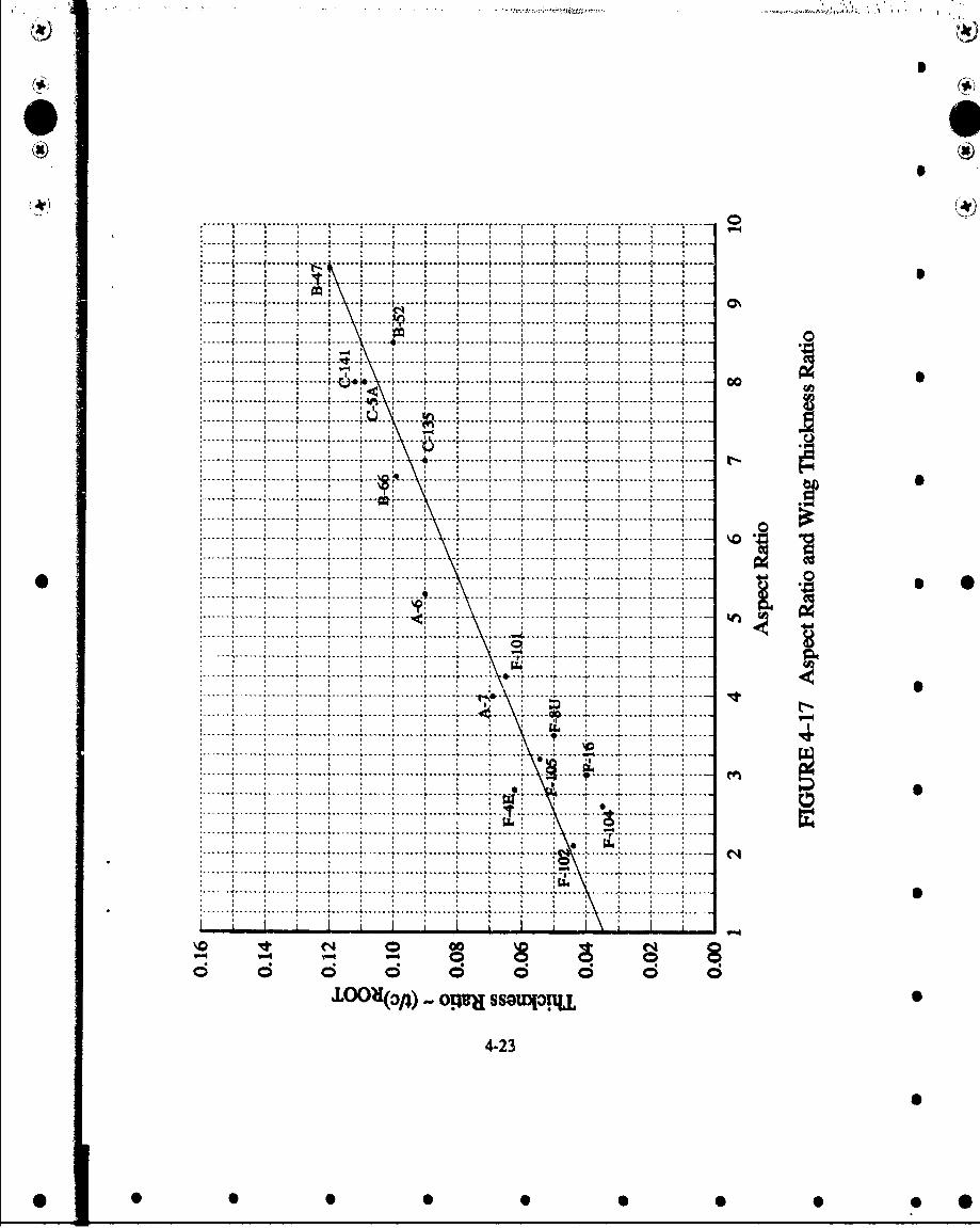
Step 15 - Determine the wing aspect ratio from Figure 4-15.
AR = 3.0
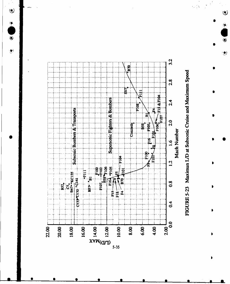
Step 16 - Estimate the maximum L/D from Figure 5-23 at a cruise speed of Mach= 0.9.Values for fighter. typically vary from 10 to 11. Select L/D= 11 mpresentativeof the F-15 and F- 16. The aspect ratio may then be chocked using figure 5-21 fora conventionally shaped fighter.
AR - 3.0
The values for aspect ratio from step 15 and 16 compare favorably and (oVe canproceed with the evaluation.
7-5
0 0 * o 0 * 4a
0 S S S S 0 O. . 3 _
Step 17 - Determine the wing thickness ratio from Figure 4-17 for an AR= 3 wing.
"t - 0.055 or 5.5% A)C
Step 18 - Compute the wing loading at take-off.
GTOW = 36,000lbs
Sjvjv -= 400ft2
W 90bs
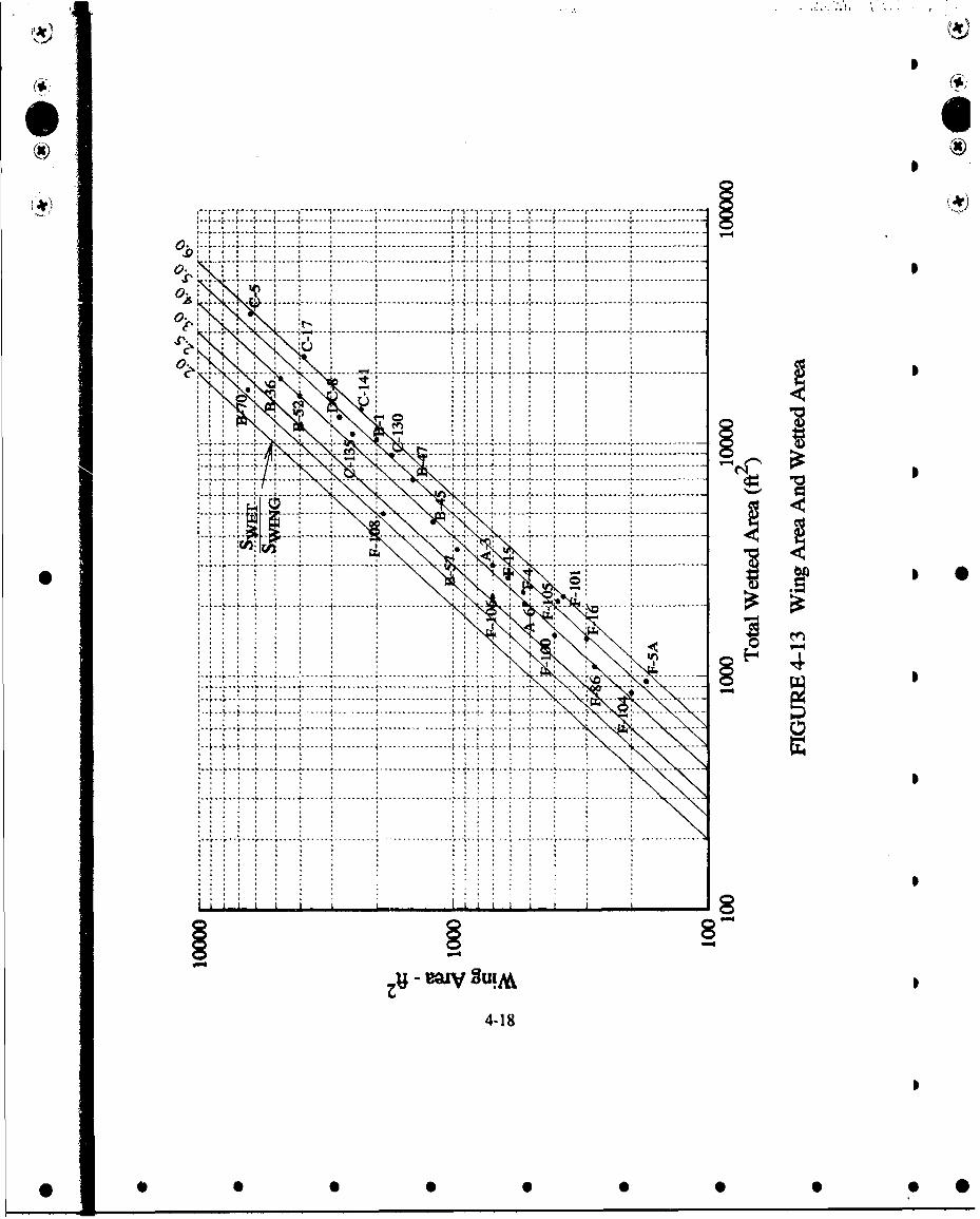
Step 19 - Determine the span loading ftomr Figure 4-14.
AR 3.0
w
W-=o30psf
S
b2
The span loading may also be computed from the relationship:
AR WI
7-6
0 00 00 0 0 0
Step 20 - Determine wing planform from Figure 4-18 for a 36,0001b fighter.
b GTOW = 36,000 (from span loading equation)4'. W 30b b2
-34.6
CTAssume a wing taper ratio, = 0.2, which is representative for a fighter.
CR = (2S By rearanging equation from Figure 4-18
Ce= 19.30ft
then C7= 3.86ft
A wing planform can now be generated to reflect a wing, A/'= 49, Ci= 19.30ff,C7= 3.86ft, and b= 34.6f.
Step 21 - Determine the size of the horizontal tail using Figure 4-19 and a preliminary 3view drawing to estimate IHT for a fighter.
Since C = ( + CT CRCT
=13.3ft
anl Sw = 13.3x400
-= 5,320fl3
then tosfJ = 1,450ft3
and s/if -1,450
If a value for Ittr can not be 6etermined, assume the horizontal tail area is 20%of the wing area. This is a non*al value and satisfactory for this stage of thedesign cycle.
7-7
• • •• • • •• •
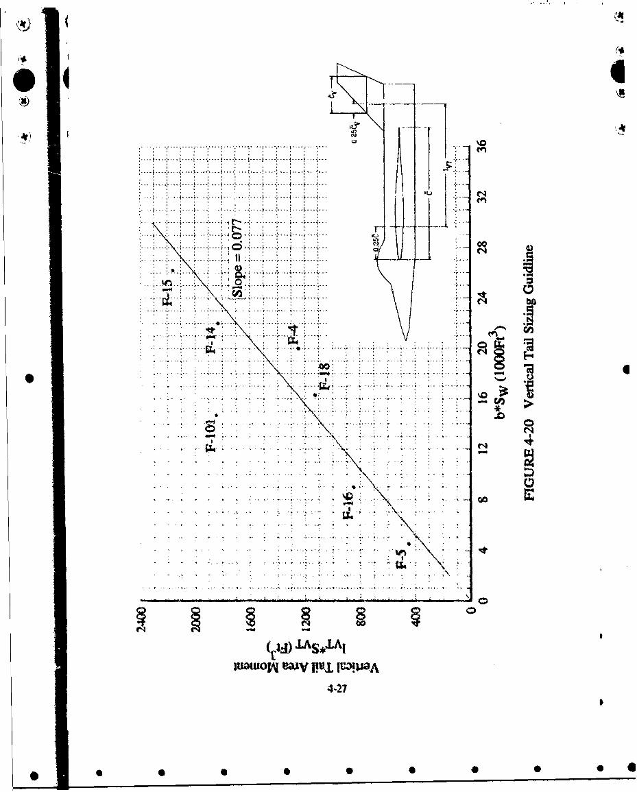
Step 22 - Determine the size of the vertical tail using Figure 4-20 and a preliminary 3-viewdrawing to estimate IVT for a fighter.
bSw = 34.6x400
,1 = 13,840ft 3
then IVTSVT = 1,070ft3
and 8VT=- 1,070
If a value for Iv can not be determined, assume the vertical is 20% of the wingarea. This is a nominal value and satisfactory for this stage of the design cyclk.
Step 23 - Determine the subsonic zero lift drag, CD0, from figure 5-10. Based on otherfighter aircraft assume an equivalent skin friction coefficient of 0.004.
For SwT = 1,972.ft2
f = CfeSwET = CDOSREFf = O.004x 1,972
= 7.89
then Cw f
7.89400
- 0.0197
Step 24 - Determine wing efficiency factor from Figure 5-8.
For AR= 3.0, e- 0.85
7-8
* 0 0 0 • S 0 0 • 0 0
Step 25 - Determine the maximum lift-to-drag ratio from Figure 5-19 or using the followingrelationship:
L 1
MAX 2 CDOK
where K =1irARe
= 0.125
and CDO = 0.0197
then L 10.1
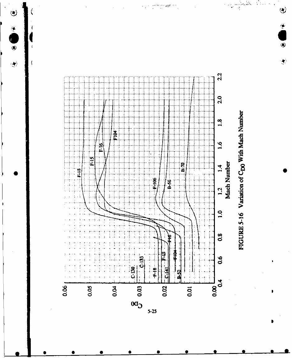
Step 26 - Determine the transonic drag rise at M= 1.2 from Figure 5-14.
For L = 55ft, de = 6.77ft, -= 0.055, A, = 490 , thenC
SL~ -L =11.24de tic 57.3
and from Fig 5-14 CDO m.12 - 2 .15 CDOsVMsO.c
- 2.15 (0.0197)- 0.042
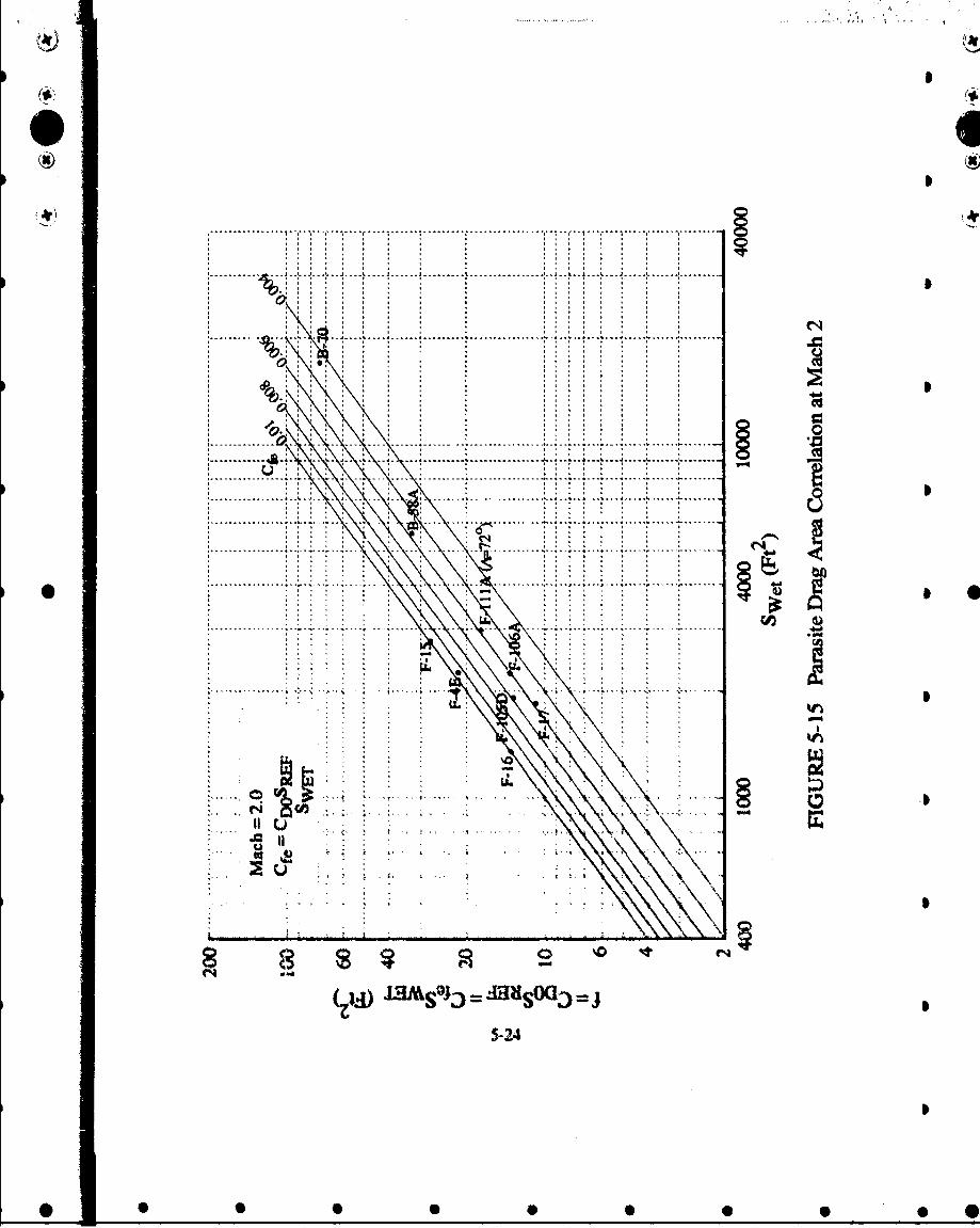
Step 27 - Determine the zero lift drag at Mach 2 from Figure 5-15. Based on other fighteraircraft assume a supersonic equivalent skin friction coefficient of 0.008.
For SwET = 1,972ft2
f = 0.008.1,972 15.7715.77
ad COo= 400
= 0.039
7-9
• • •• • • •• o
Il 0~ mm e••g 0 0 • 0 0 0 0 ,0 0J
* 0 0 S 0 O0 .' O O
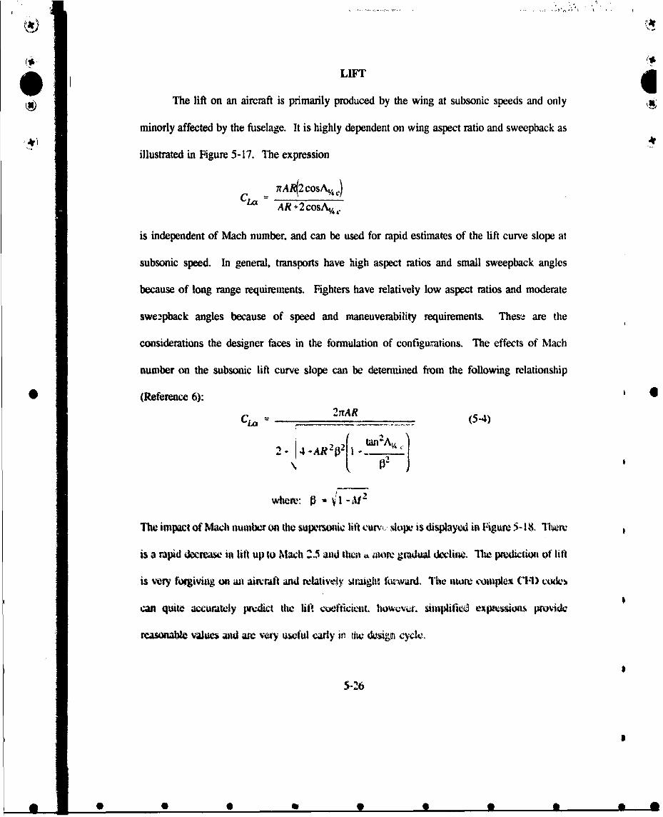
Step 28 - Determine the subsonic lift curve slope from Figure 5-17
0 For ALjE 490, Cie= 19.30ft, C7= 3.86fl, and b= 34.6ft
then Ay,-= 420 and AR= 3.0 and from Fig 5-17
C L a t = 3.2 r
= 0.056deg
Step 29 - Determine the optimum lift coefficient for cruise flight from the relationships onpage 5-29:
CDOCL OPT ~F where K= 0.125 from step 25
=i0.0197
\0.125
- 0.397
Step 30- Determine the 2T ratio for this postulated fighter from figure 3-4, TW W
required at take-off for a highly agile fighter for the maneuverability specified willWapproach current inventory aircraft. For a -S . 90, assume a minimumS
Trequirement of T = 1.0. This value may have to be iterated if our aircraft does
Wnot meet the specifiod maneuverability goals.
Step 31 - Determine the inaximum lift coefficient from figure 6-1.
For A,,.E 494 ; CLm\,c 1.5
7-10
O O0 0 V O 0' '0
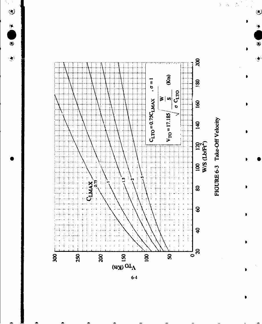
Step 32- Determine the take-off distance from Figures 6-4.
wFor A =490 , CLan1.5, d 90psf
L LMAX =S.5
"VTO = 155knots from figure 6-3
then -=80(T=
T)
w,ýere we assume T = 1.0w
and Ca.o = 1.1.5 (CLTO=75 % CLMAX)
Take -Off Distance = 1,2001f
Step 33 - Determine the approximate cruise range at Mach 0.9 and 30,000fi from Figure 6-7
or the relationship:
R 2.3_V L..-05SFC WFMAL•
132oM A)R =LogWINM
SFWF L
Where I L GTOW - 3 0%(WFUE1)
wh•r ZTOW - 7O%(WFUU)
36,000 - (0.3)(9,730)36,000 - (0.7)(9,730)
= 1.133
and SFC = 1.0 at M 0.9; L/D 10.1; IVF, =9,730lbs
then R 651ni.
7-11
m •
* 0 0 O O O 0 O, "*
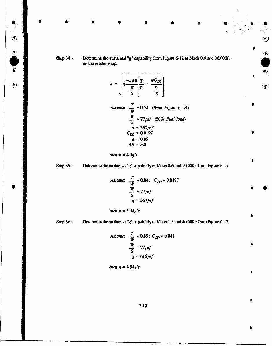
Step 34 - Determine the sustained "g" capability from Figure 6-12 at Mach 0.9 and 30,000ftor the relationship.
n reAR T qCD,
T
Assume: T = 0.52 (from Figure 6-14)W
S-- 77psf (50% Fuel load)Sq = 360psf
CDO = 0.0197e = 0.85
AR = 3.0
then n = 4.0g's
Step 35 - Determine the sustained "g" capability at Mach 0.6 and 10,000ft from Figure 6-I1.
Assume: T = 0.84; CDo,= 0.0197• w- = 77psfSq = 367psf
then n = 5.34g's
Step 36 - Determine the sustained *g" capability at Mach 1.5 and 40,00ft from Figure 6-13.
A,vume: w . 0.65, CtX=- 0.041W-- u77psfSq - 616psf
then n = 4.54g's
7-12
! • ml m w .. • m • • • • m . • • m u • • l m m , l u r ll • w m • • • m m m u =w i •
S0 0
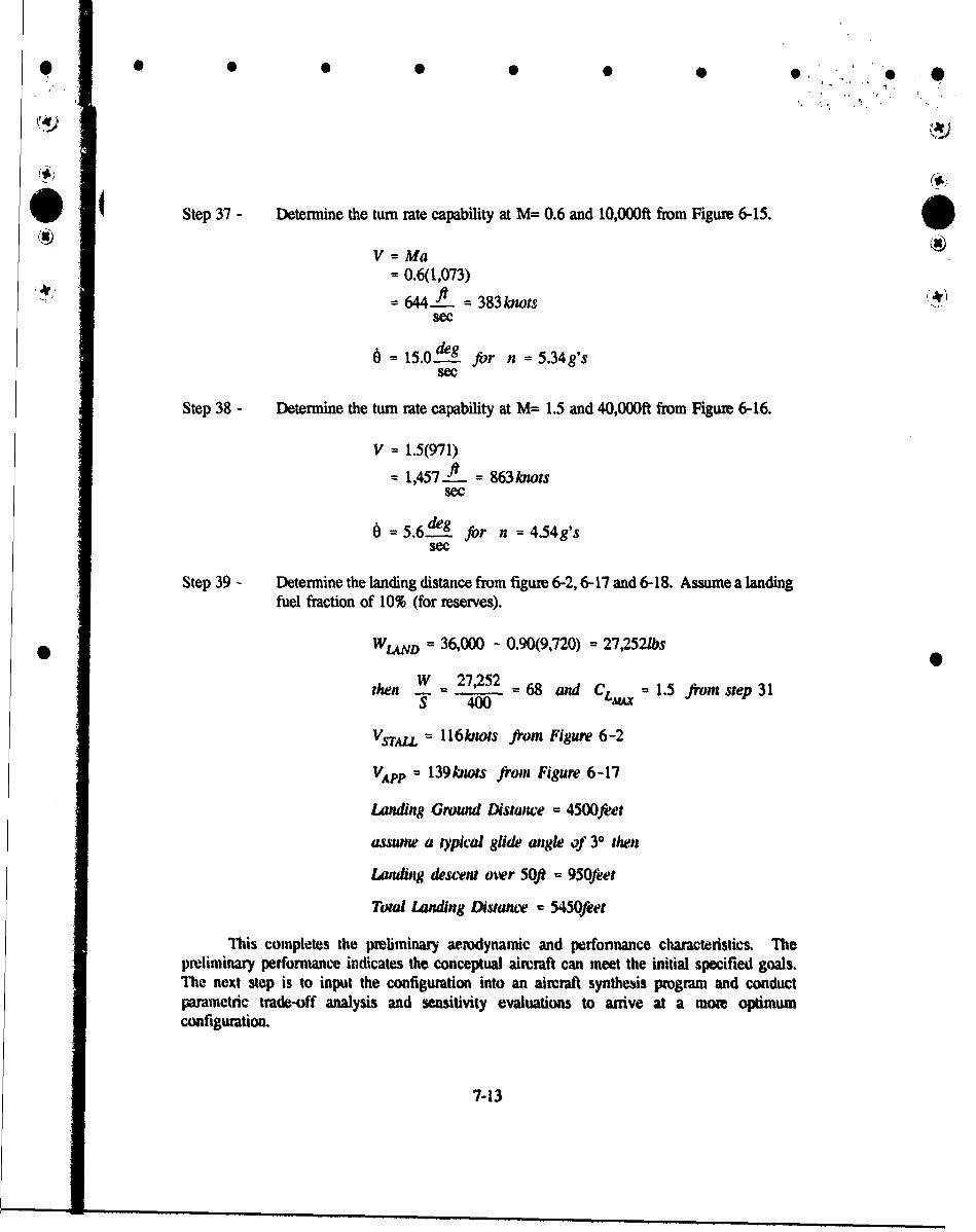
@ 4Step 37 - Determine the turn rate capability at M= 0.6 and 10,OO0ft from Figure 6-15.
V = Ma= 0.6(1,073)
= 644 fA = 383knotssec
0= 15.0deSgi for n = 5.34g's
sec
Step 38 - Determine the turn rate capability at M= 1.5 and 40,000ft from Figure 6-16.
V = 1.5(971)
= 1,4571 = 863knotssec
= 5.6.dg for n = 4.54g'ssee
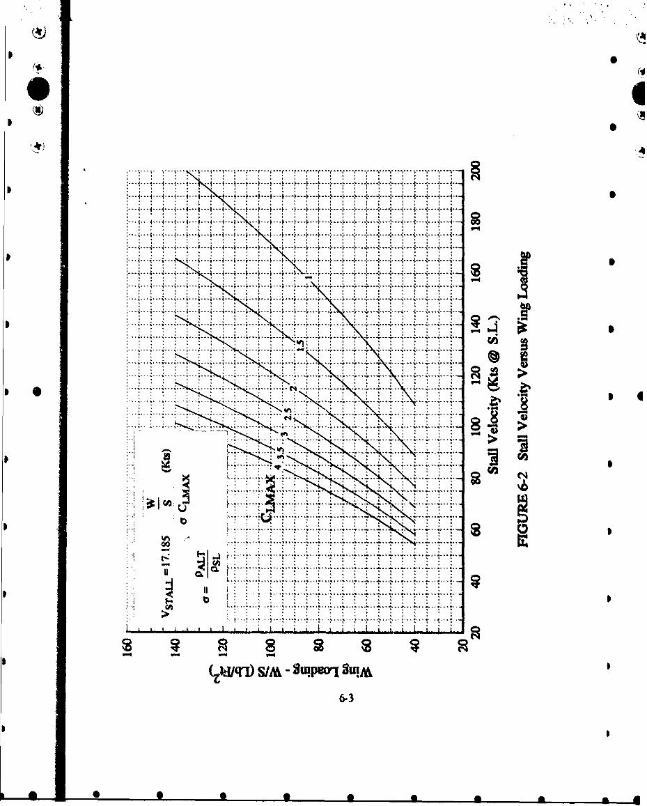
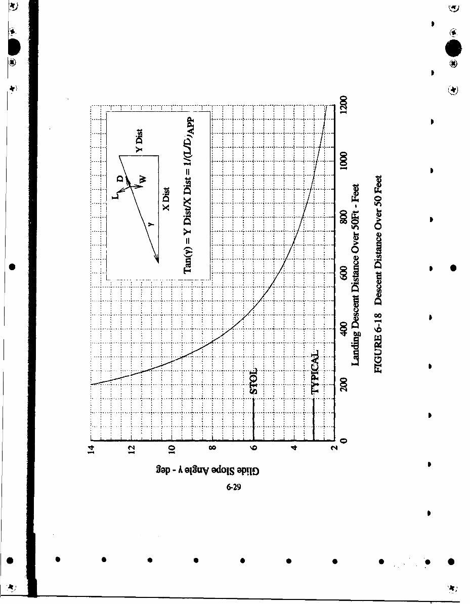
Step 39 - Determine the landing distance from figure 6-2,6-17 and 6-18. Assume a landingfuel fraction of 10% (for reserves).
* WLjVD = 36,000 - 0.90(9,720) = 27,252/bs
then W 27,252 = 68 wa CL 1.5 from step 31S= 400 L
VsrAU" = 116ksnos from Figure 6-2
VApe = 139 nowts ftom Figure 6-17
Landing Ground Distance = 4500feet
assume a typical glide angle of 30 then
Laiuling descent ovwr 50ft = 950feet
Total Landing Distance - 5450ftet
This completes the preliminary aerodynamic and perfontance characteristics. Thepreliminary perfomance indicates the conceptual aircraft can meet the initial specified goals.The next step is to input the configuration into an aircraft synthesis program and conductparametric trade-off analysis and sensitivity evaluations to arrive at a more optimumconfigumtion.
7-13
* 0 0 0 0 , " 0*9
I
O4,
*. CONCLUSIONS
This report provides design data and procedures to initially formulate and analyze an aircraft
configuration. It is based on an array of data from past military aircraft. Many convenient charts
are included to rapidly define pertinent features of a configuration, and to evaluate their impact
on the lift and drag characteristics.
The design data and procedures can be used to perform the following tasks:
• Size and shape initial fighter and transport configurations.
• Estimate gross-take-off weight, empty weight and fuel weight.
• Define fuselage fineness ratio and wing geometry.
* Size horizontal and vertical tails
• Estimate aircraft wetted area and volume
• Determine pertinent aircraft configuration parameters such as wing loading,
span loading and thrust loading.
* Predict the drag characteristics at subsonic, transonic and supersonic speeds
• Predict lift curve slope across Mach range
• Estimate naximum lift-to-drag ratio
* Assess performtnce capability of conceptual aircraft
8-1
S
9. REFERENCES
1. Nicolai, Leland M., "Fundamentals of Aircraft Design", METS, Inc, San Diego, CA, 1984.
2. Raymer, Daniel P., "Aircraft Design-A Conceptual Approach" AIAA, Washington D.C.,1989.
3. Rinn, S. "CASP Preliminary Sizing Program Wright Laboratory, Wright-Patterson AFB,Ohio, 1989.
4. Hollowell, S. et al, "Interactive Design and Analysis System", N.A. 82-467, RockwellInternational, Los Angeles CA, 1982.
S
5. Schemensky, R.T., "Development of an Empirically Based Computer Program to PredictThe Aerodynamic Characteristics of Aircraft," AFFDL-TR-73-144, Wright- PattersonAFB, Ohio 1973.
6. Ellison, D.E., "USAF Stability and Control Handbook, (DATCOM)", Air Force FlightDynamics Laboratory, Wright-Patterson AFB, Ohio, Revised 1976.
7. Perkins, Courtland D. and Hage, Robert E., Airplane "Performance, Stability and Control,"John Wiley & Sons Inc, September 1954.
8. Wood, K.D., "Aircraft Design", Johnson Publishing Co., Boulder, Colorado, 1966.
9. Roskam, j., "Airplane Design", Parts I to VIII, Roskam Aviation & Engineering Corp.,Ottawa, Kansas, 1989.
S10. Genston, W., "The Encyclopedia of World Air Power," Crescent Book, Crown Publishers,
Inc., 1986.
II, Taylor, U.W.R., "Janes All The World Aircraft," Janes Publishing Co, London, England,1984.
12. Aviation Week & Space Technology," 1992 Aerospace Forecast," Vol. 136. No. 11, NewYork, N.Y. March 16, 1992.
13. Coming, Gerald. "Airplane Design", Edwards Brothers, Inc, Ann Arbor, Michigan. 1953.
14. Caddell, WKE., "On the Use of Aircraft Density In Prelitninary Design", SAWE Paper No.813, 5 May 1969.
15. Abbot, 1.11., "Theory of Wing Sections," Dover Publications, hic., 1959.
9-1
LS
* 16. Abbot, I.W., "Characteristics of Wing Sections," NACA TR 824, 1945.
17. Jones, R.T., "Properties of Low Aspect Ratio Wings", NACA TR-835, 1946.
18. Johnson, M.E., "Design and Analysis of Maneuver Wing Flaps at Supersonic Speeds,"
NASA CR-3939, 1985.
19. Hoemer, S.F., Fluid Dynamic Drag," Midland Park, New Jersey, 1965.
20. Ely, W.E. et el, "Prediction of Aircraft Drag Due to Lift," Air Force Flight DynamicsLaboratory, AFFDL-TR-71-84, Wright-Patterson AFB, Ohio, June 1971.
21. Gollos, W.W., "Transonic and Supersonic Pressure Drag for a Family of Parabolic TypeFuselages at Zero Angle of Attack," Rand RM 982, 1952.
22. Morris, D.N., "A Summary of the Supersonic Pressure Drag of Bodies of Revolution",Journal of Aeronautical Sciences, Vol, 28, July 1961.
23. Nelson & Welsh, "Application of the Transonic & Supersonic Area Rule to the Predictionof Wave Drag," NASA TN D-446, September 1960.
24. Mirels, H., "Aerodynamics of Slender Wings and Wing Body Combinations Having SweptTrailing Edges", NACA TN-3105, 1954.
0 25. Hall, C.F., "Lift, Drag and Pitching Moment of Low Aspect Ratio Wings," NACA RMA53A30, 1958.
26. Carlson, H.W. and Mann, MJ.. "Survey and Analysis of Research on Supersonic Drag-Due-ToLift Minimization with Recommendations for Wing Design," NASA Tech Paper3202. 1992.
27. Harris, R., "An Analysis and Correlation of Aircraft Wave Drag," NASA TM X-947.1964.
28. May, F. and Widdison, C.A., "STOL High Lift Design Study" AFFDL TR-71-26, WrightPatterson AFB. Ohio, April, 1971.
29. Bonner, E. and Gingrich, P., "Supersonic Cruise.lransonic Maneuver Wing SectionDevelopment Study," AFWAL-TR-80-3047, Wright Pa-wum AM, Aiu, I r.9.
30. Carlson, 11. and Miller, D., "Numerical Methods for the Design and Analysis of Wingsat Supersonic Speeds," NASA "IN D)-7713, 1947.
9-2
* S S 0 0 S • "
31. Miller, D., "Supersonic Wing Design Concepts Employing Non-Linear Flows,' 14th ICASProceedings, 1984. - lt
32. Miller, D. and Schemensky, R., "Design Study Results of a Supersonic Cruise Fighter 4Wing", AIAA Paper 79-0062 1979.
33. Etkins, Bernard, "Dynamics of Atmospheric Flight," John Wiley & Sons, 1972.
34. Rutowski, E.S., "Energy Approach to the General Aircraft Performance Problem," Journalof Aeronautical Sciences, March 1954.
35. Bryson, A.E. and Desai, M.N. "Energy State Approximation in Performance Optimizationof Supersonic Aircraft", Journal of Aircraft, Vol. 6, November 1969. S
9-3
S
SS .... 00
APPENDIX A!P A)
Representative Operational and Advanced Configurations
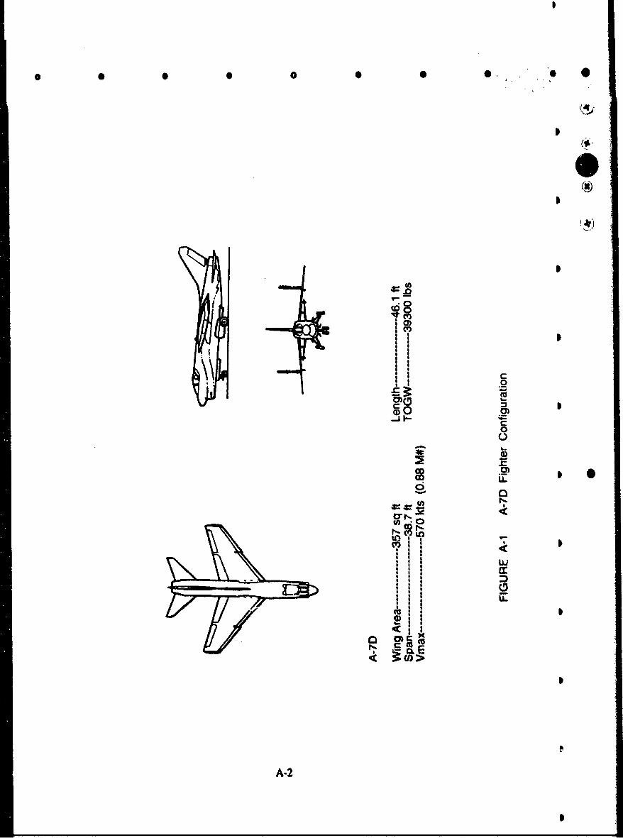
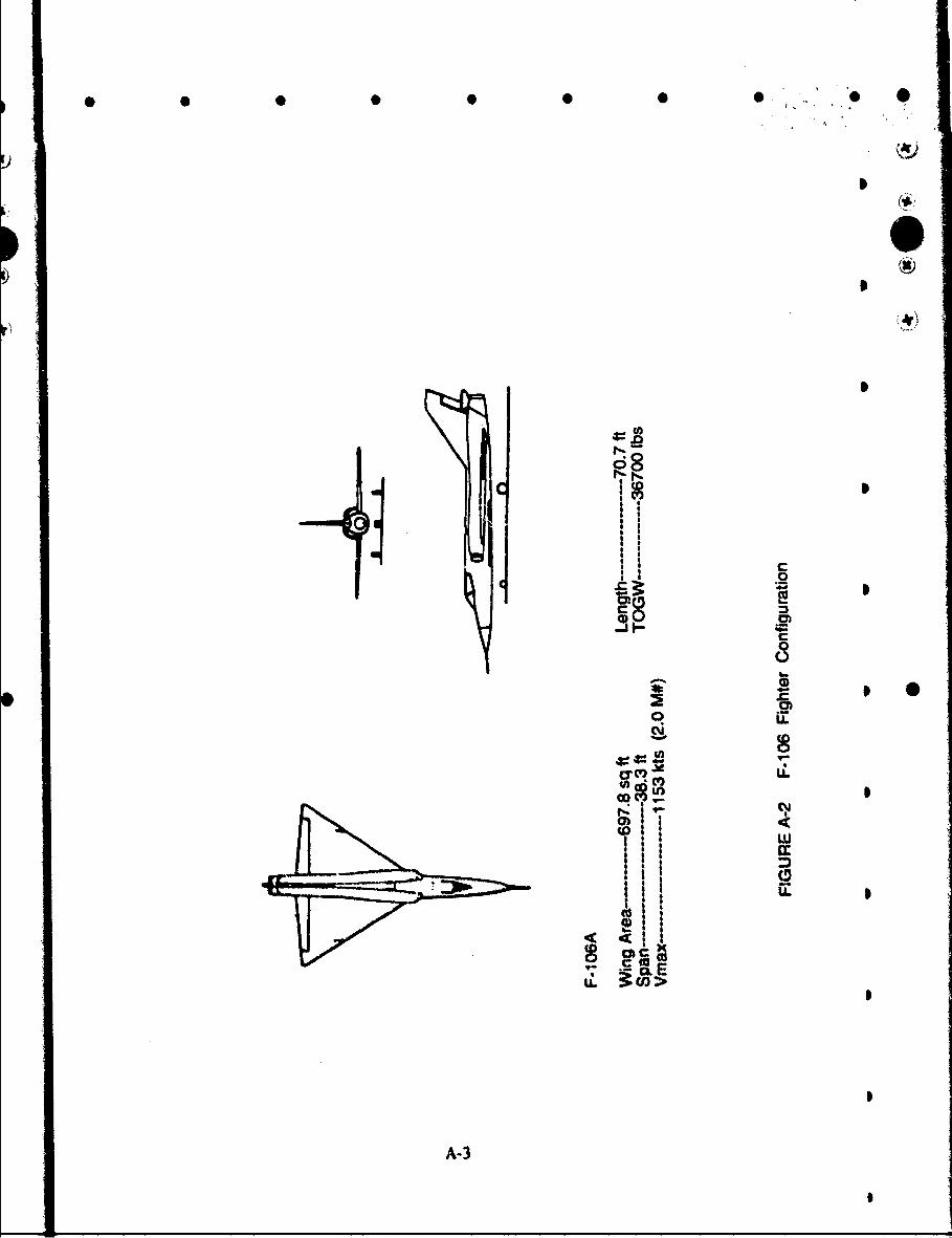
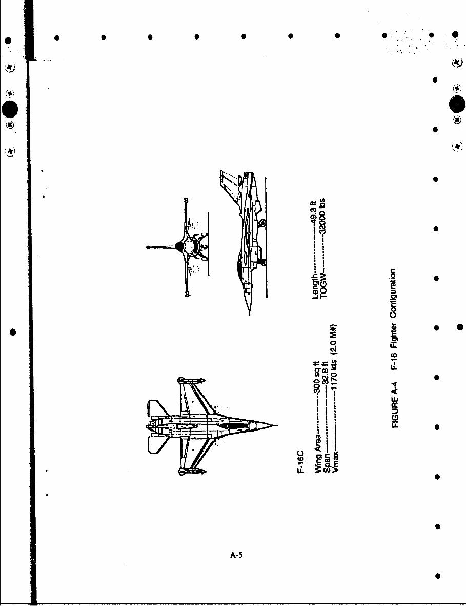
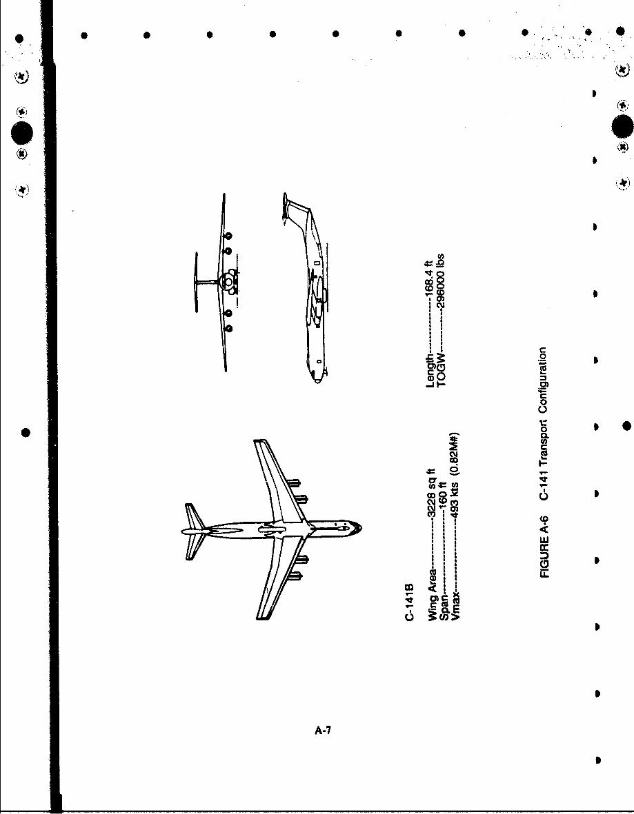
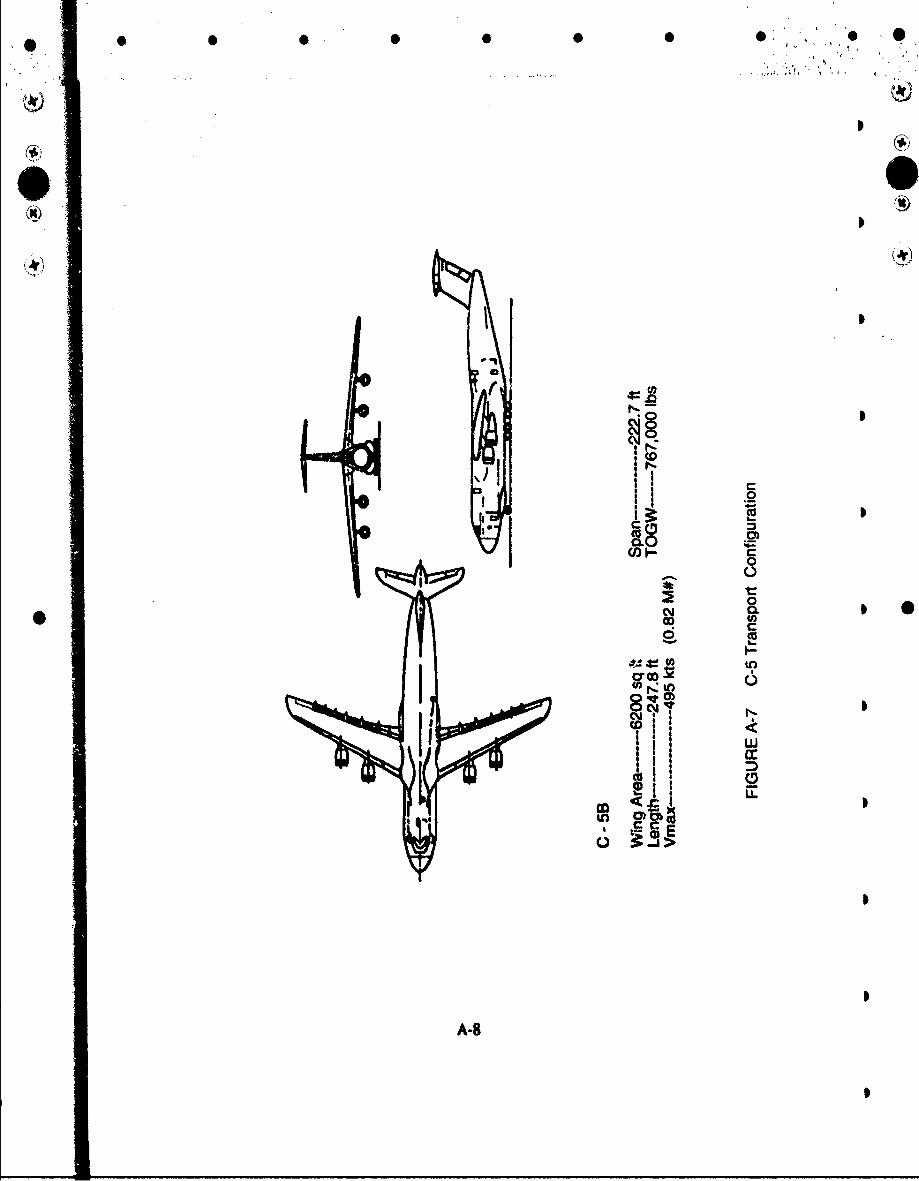
This appendix is composed of 3-view drawings of several current and advanced military
aircraft. Each drawing contains the wing aria, span, length gross take-off weight and maximum
speed. It is to illustrate the size and shape of aircraft configurations based on specific
performance requirements.
A
A-I
• • •• • • •• •
* 0 0 0n• •• w 0 0 0 0 J 0 0 0 ~
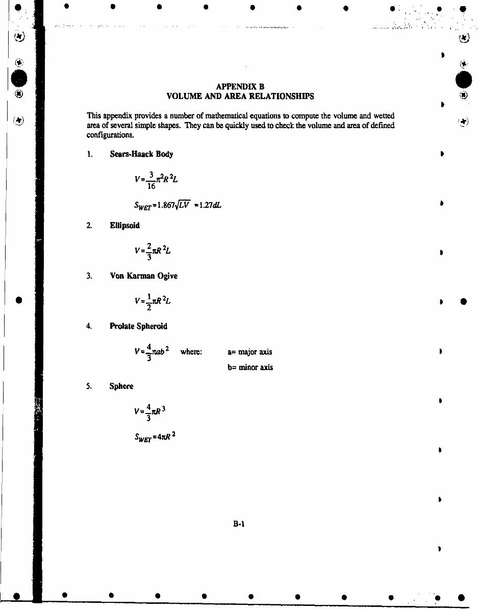
APPENDIX B_• VOLUME AND AREA RELATIONSHIPS
This appendix provides a number of mathematical equations to compute the volume and wettedarea of several simple shapes. They can be quickly used to check the volume and area of definedconfigurations.
1. Sears-Haack Body
V=I X2R 2L
16
SwE= 1.867L"V" =1.27dL
2. Ellipsoid
V=2..J 2L3
3. Von Karman Ogive
0 V--�t R2L * *2
4. Prolate Spheroid
V=1=ab0 where: a- major axis3
b= minor axis
5. Sphere
vi&3
Sw••4tR 2
S~B-I
,O, • •• •• • e
* ....0 0 0mmWm~~wwmme.mwm m S S S • S~em S•emmm•mm 0m• m~ u 0
6. Right Cone
V=I!R 2L
3
SwEgrT% R'O+L' (Curved Surface)
7. Right Cylinder
V=id?2L
SwET= 27xRL (Curved Surface)
8. Cone Frustrum
V= IE (R 2+R R +R 2)
SWET ='[2(RI R4 2) +2(1 -R2)2 (Curved Surface)
Where: RI= Radius of BaseR2= Radius of TopL= Length
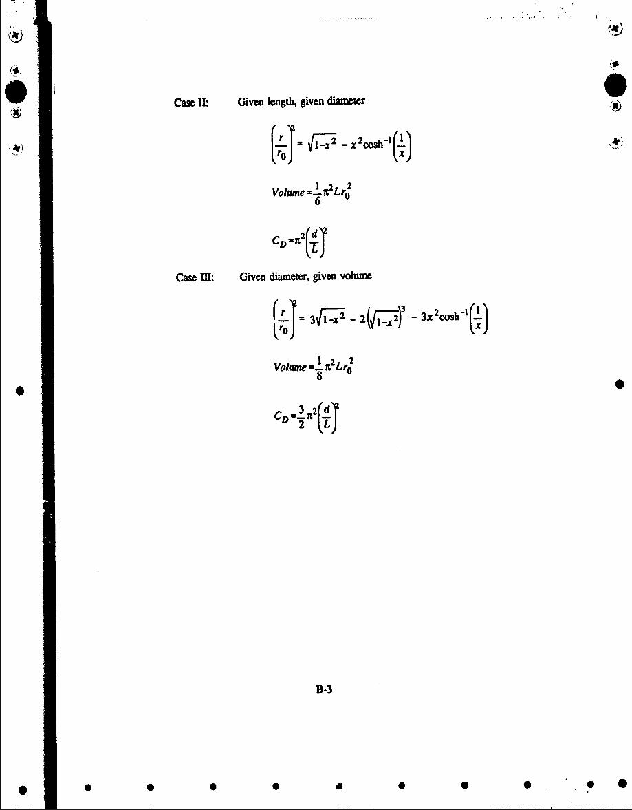
9. Formulas for Sears.Haack body of revolution shapes, volume and drag
The factor d/L is the fineness ratio, diameter/length.I
Case I: Given length, given volume
(i~~)
valumme n2LP
T6
C D O 1 , d
B-2
• • •• • • •• o
*ie l mlili lmi m m 4 ~ l I i • ll l l , . 0 M iii mi
Case II: Given length, given diameter W
(70- (71)
6Vro
Case I1l: Given diameter, given volume
3 2 .X2- 2 _2)- 3x cosh, -..
Volume • r8 r
2 0T
B-3
0 0 • • 0 0 • 0 0•
APPENDIX CWINGS IN SUPERSONIC FLOW
Based on linear, two dimensional (2-D) supersonic flow theory (References 5 and 6), the
pressure coefficient in wpersonic flow can be related to the flow turning angle, A6, such that
±2A(
FM i(C-i)
where AO is illustrated iz, sketch A.
V00
tI
->
SKETCH A
SA 2-D airfoil at angle of attack can be repesented by a flat plate at angle of attack, a mean 0
camber line, and a symmetric thickness distribution as indicated in sketch B below.
+ +
Alpha Camber ThicknessI
SKETCH B
Integration of the pressure from equation (C-I) in the drag direction yields
L ,4 + 3 (C-2)
forth three c ponp enu of alpha, camber, and thckes respectively. The second pat of this
C-I
• • •• • • •• •
* " S" ' 5: "' ,.. . "'" 0 i 0 0•.. " l' -i 0-r •
equation is the profile wave drag due to camber and thickness. The minimum profile drag occurs jfor a symmetrical wedge shape, and results in K2= 0 and Kr= (t/c)2 so that
CDWAV" 4l (C-3)
The first term is the wave drag due to lift and is somewhat similar to subsonic induced drag.
The second term is the wave drag due to thickness and indicates the extreme importance of
keeping wings thin on supersonic aircraft. The dependence on Mach number is also indicated
in the equations.
The wave drag due to lift term from equation C-3 can be expressed as
CDw =KC2 where K= 1 . for M>ILAV KCL
The above expression is often used as an asymptotic limit for wings at higher Mach numbers.M 5@
Integration of the pressure in equation C-1 in the lift direction yields4ct
CL = 4 (C4)
or
dCL 4 4
If we ignore friction drag %ve can combine the equation for CL and CD, form CL/CO.
differentiate and establish the maximunm (LAD) ratio for a 2.D wedge
LMAX 4 j
Which oaeagain indicates the importanc of thin shapes at supersonic speeds.
C-2
• • •• • • •• •
0 .. .. . "0 S °" i - - 0-I... l 'l ii • 0 . .i ' I0[i 1*"i .... 0i ...
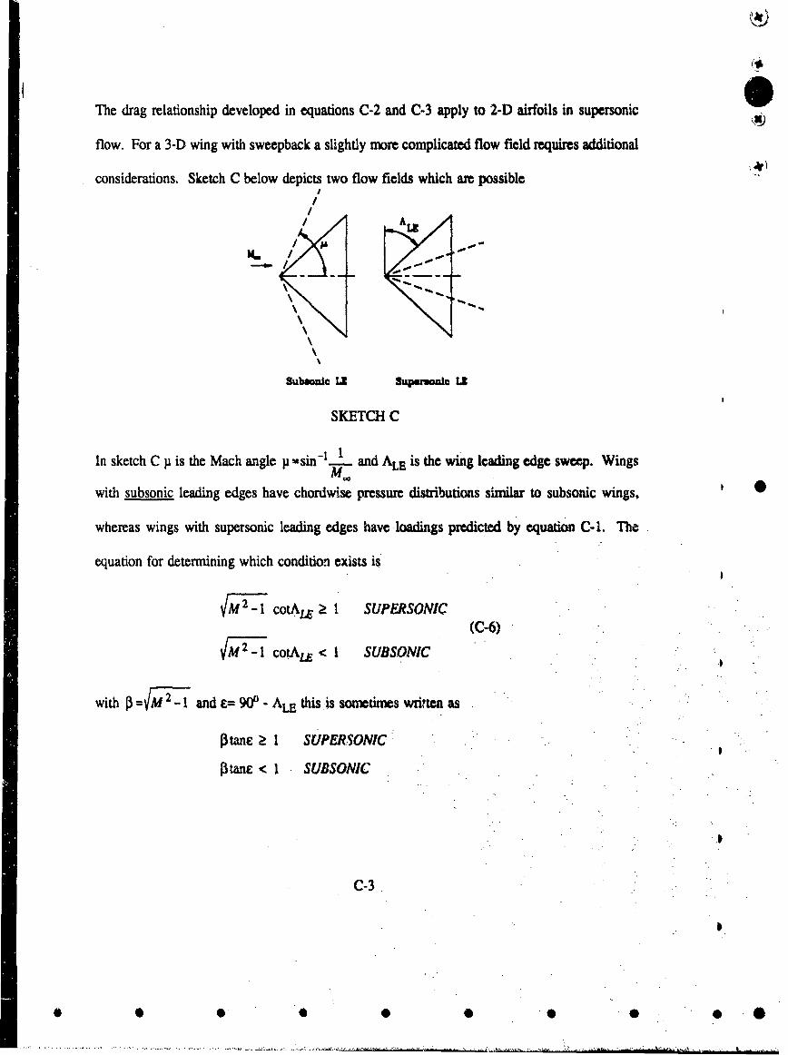
The drag relationship developed in equations C-2 and C-3 apply to 2-D airfoils in supersonic
flow. For a 3-D wing with sweepback a slightly more complicated flow field requires additional
considerations. Sketch C below depicts two flow fields which are possibleI
/- /
II
Subsonaic Ll SupewMonic LZ
SKETCH C
In sketch C p is the Mach angle p =sin-.'.1 and ALE is the wing leading edge sweep. Wings
with subsonic leading edges have chordwise pressure distributions similar to subsonic wings, 0
whereas wings with supersonic leading edges have loadings predicted by equation C-1. The
equation for determining which condition exists is
FM7_- cotAE 2! 1 SUPERSONIC(C-6)
FM -ý cotALE < 1 SUBSONIC
with FM - and E= 90P - ALE this is sometimes written as
Jtane a I SUPERSONIC
PtanE < I SUBSONIC
C-3
0 O 0 0 0 "O O0 0
The wave drag of uncambered and untwisted trapezoidal wings can be estimated by
CW) t FOR PcotAS > 1
=Ktane FOR IcontA, < 1
withK= 16/3 for biconvex airfoils
K= 4 for double wedge airfoils
Note that the upper expression is identical to the 2-D wedge shape in equation C-3.
The above expressions are for ballpark estimates only and do not capture many of the
finer details that determine wing wave drag. Leading edge bluntness, aspect ratio, camber and
location of maximum thickness are all important parameters which can significantly effect wing
S wave drag.
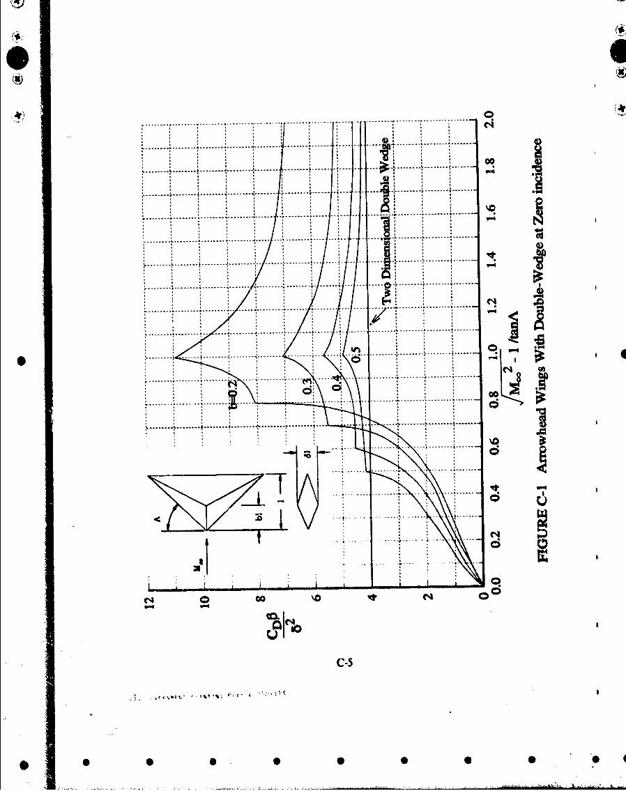
Referring to Figure C-1 the following observations are made. Above PcotALE > 1 where
the wing leading edge is supersonic the drag is shown to be a strong function of the chordwise
location of maximum thickness, "b" in Figure C-1, and approaches the (2-D) symmetric wedge
value given by equation C3 (CL= 0) at higher Mach numbers. The curve is altered between
PcotAtE > I and an abscissa value that represents the sweep of line of the maximum thickness.
For example, for b=0.3 this value PcotAL= 0.7 which represents where the sweep angle AO;
becocues subsonic in an analogous marner to the leading edge. At lower Mach numbers the
location of optimum chordwise thickness reverses and minimum drag is represented by nmre
formwid thickness distributions characteristic of subsonic flows.
C-4
0 0 O O 0 0- *•