ADDIS ABABA UNIVERSITY
ETHIOPIAN INSTITUTE OF WATER RESOURCES
MSc THESIS ON
Runoff Estimation and Water Management for Holetta River,
Awash subbasin, Ethiopia
By:
Mahtsente Tibebe
June, 2013
II
In
An MSc Thesis on:
Runoff Estimation and Water Management for Holetta River,
Awash subbasin, Ethiopia
Submitted By:
Mahtsente Tibebe Tadese [email protected]/ [email protected]
Supervised By:
Dr. Assefa Melesse - Florida International University
Dr. Dereje Hailu - Addis Ababa University
Dr. Birhanu Zemadim - International Water Management
Institute
June, 2013
Addis Ababa, Ethiopia.
Addis Ababa University P.O.Box 1176, Addis Ababa, Ethiopia T +251-11-1239 768 F +251-11-1239 752 I www.aau.edu.et
Ethiopian Institute of Water Resources
P.O.Box 150461, Addis Ababa, Ethiopia T +251-11-1223 344 F +251-11-1239 480 E [email protected]
Mahtsente Tibebe Tadese MSc Candidate
“BU
ILDI
NG
ETH
IOPI
A’S
WAT
ER F
UTU
RE
TOG
ETHE
R”
III
Runoff Estimation and Water Management for Holetta River,
Awash subbasin, Ethiopia
Thesis Submitted to Ethiopian Institute of Water Resources in Partial Fulfilment of the Requirements for the Degree of Master of Science
In
Water Resources Engineering and Management (Specialization: Surface Water Hydrology)
By Mahtsente Tibebe Tadese
APPROVED BY BOARD OF EXAMINERS
Dereje Hailu (Dr.) --------------------------------------- ------------------------------------ (Main Advisor) Signature Date Birhanu Zemadim (Dr.) --------------------------------------- ------------------------------------ (Co- Advisor) Signature Date Assefa Melesse (Dr.) --------------------------------------- ------------------------------------ (Co- Advisor) Signature Date Agizew Negusue (Dr.) -------------------------------------- ------------------------------------- (External Examiner) Signature Date Seifu Kebede (Dr.) -------------------------------------- ------------------------------------- (Internal Examiner) Signature Date Rahel Eshetu (MSc.) -------------------------------------- ------------------------------------- (Chairman) Signature Date
IV
Declaration I hereby certify that I have prepared this MSc thesis independently, and that only those
sources, aides, and advisors that noted herein have been used and/or consulted. I declare that
this thesis is my work and that all sources of materials used for this thesis have been duly
acknowledged.
................................................ ......................................................... Signature: Mahtsente Tibebe Tadese Date (MSc Candidate)
V
ACKNOWLEDGMENT
At first, I would like to thank my almighty God, being there for me on every second in life.
Next, I am highly gratitude to my advisors for their valuable guidance and support in my
entire research work. I also want to express my deepest thank for Holetta Research Center,
Ministry of Water and Energy, Ethiopian Institute of Water Resource and United States
Agency for International Development (USAID) /HED for all their support.
Finally yet importantly, my heartfelt thank goes to all my family and friends, specially my
husband for your encouragement and wonderful support.
VI
ACRONYMS AND ABBREVIATIONS AAU Addis Ababa University
AGRC Agricultural Land -Close-Grown
AGRR Agricultural Land- Row Crops
ARS Agricultural Research Service
CWR Crop Water Requirements
DEM Digital Elevation Model
FAO Food and Agriculture Organization of the United Nation
ETo Reference Evapotranspiration
FRSD Forest -Deciduous
FRST Forest-Mixed
GIS Geographical Information System
HARC Holetta Agricultural Research Center
HRUs Hydrological Response Units
IR Irrigation Requirement
IVF Index of Volumetric Fit
Kc Crop coefficient
LH-OAT Latin Hypercube One-factor-At-a-Time
NSE Nash-Sutcliffe Efficiency Coefficient
SCS Soil Conservation Service
SWAT Soil and Water Assessment Tool
USDA United State Department of Agriculture
WETL Wetlands-Mixed
WMO World Meteorological Organization
VII
TABLE OF CONTENTS ACKNOWLEDGMENT ....................................................................................................... V
ACRONYMS AND ABBREVIATIONS .............................................................................. VI
TABLE OF CONTENTS..................................................................................................... VII
LIST OF FIGURES .............................................................................................................. XI
LIST OF FIGURES IN THE APPENDIX ........................................................................... XII
ABSTRACT ...................................................................................................................... XIII
1. INTRODUCTION .............................................................................................................. 1
1.1. Background and Justification........................................................................................ 1
1.2. Problem Statement ....................................................................................................... 2
1.3. Research Questions ...................................................................................................... 3
1.4. Objectives .................................................................................................................... 3
1.5. Significance of the Study .............................................................................................. 4
1.6. Structure of the Thesis .................................................................................................. 4
2. LITERATURE REVIEW ................................................................................................... 5
2.1. Global Water Management and Allocation Issues ......................................................... 5
2.2. Hydrological Models .................................................................................................... 6
2.3. Description of SWAT Model ........................................................................................ 7
2.3.1. Land Phase of the Hydrologic Cycle ...................................................................... 8
2.3.2. Routing Phase of the Hydrologic Cycle ................................................................ 12
2.4. Description of CROPWAT Model .............................................................................. 12
2.4.1. Crop Water Requirement ..................................................................................... 13
2.4.2. Crop Coefficient Approach .................................................................................. 13
2.4.3. Effective Rainfall ................................................................................................. 14
2.5. Previous Study in the Area ......................................................................................... 14
VIII
TABLE OF CONTENTS (continued)
2.5.1. Design of a community based Dam in Holetta, Ethiopia ....................................... 14
2.5.2. Simulation and Optimization for Irrigation and Crop planning ............................. 15
3. MATERIALS AND METHODS ...................................................................................... 16
3.1. Description of Study Area .......................................................................................... 16
3.1.1 .Topography ......................................................................................................... 17
3.1.2. Climate ................................................................................................................ 18
3.1.3. Land use/ Land cover ........................................................................................... 19
3.1.4. Soil Classification ................................................................................................ 19
3.2. Data Collection .......................................................................................................... 20
3.3. SWAT Model Input .................................................................................................... 21
3.3.1. Digital Elevation Model Data .............................................................................. 21
3.3.2. Land Use Map ..................................................................................................... 22
3.3.3. Soil Map .............................................................................................................. 23
3.3.4. Meteorological Data ............................................................................................ 24
3.3.5. Flow Data ............................................................................................................ 26
3.4. SWAT Data Preparation and Model Setting ............................................................... 27
3.5. Sensitivity Analysis .................................................................................................... 28
3.6. Model Calibration and Validation............................................................................... 29
3.7. Model Evaluation ....................................................................................................... 30
3.8. Runoff Estimation ...................................................................................................... 32
3.9. CropWat Model Input ................................................................................................ 32
3.9.1. Climatic Data ....................................................................................................... 32
3.9.2. Rainfall Data........................................................................................................ 32
IX
TABLE OF CONTENTS (continued)
3.9.3. Cropping Pattern Data.......................................................................................... 33
3.9.4. Soil Type Data ..................................................................................................... 34
4. RESULTS AND DISCUSSIONS ..................................................................................... 35
4.1. Hydrological Analysis ................................................................................................ 35
4.1.1. Watershed Delineation and Determination of HRUs ............................................ 35
4.1.2. Sensitivity Analysis ............................................................................................. 35
4.1.3. Model Calibration ................................................................................................ 36
4.1.4. Model Validation ................................................................................................. 39
4.1.5. Runoff Estimation for Holetta Catchment ............................................................ 41
4.2. Questionnaire Analysis ............................................................................................... 46
4.3. CROPWAT Model Analysis ...................................................................................... 50
4.3.1. Reference Evapotranspiration .............................................................................. 50
4.3.2. Effective Rainfall ................................................................................................. 51
4.3.3. Crop and Soil Data............................................................................................... 52
4.3.4. Crop Water Requirement and Irrigation Requirement .......................................... 53
4.4. Water Demand Analysis ............................................................................................. 54
5. CONCLUSIONS AND RECOMMENDATIONS ............................................................. 62
5.1. Conclusions................................................................................................................ 62
5.2 Recommendations ....................................................................................................... 63
REFERENCES ..................................................................................................................... 65
APPENDICES...................................................................................................................... 68
X
LIST OF TABLES
Table 1. Ethiopian River Basin's runoff and ground water potential (Awulachew et al., 2007) 1
Table 2. Information of climate and hydrology stations......................................................... 25
Table 3. Result of sensitivity analysis of flow at Holetta subbasin......................................... 36
Table 4. Initial and final adjusted value of calibrated flow parameters at Holetta subbasin ... 37
Table 5. Summary of mean flow (m3/s) at the subbasins ....................................................... 46
Table 6. Summary of livestock which users Holetta River .................................................... 50
Table 7. Summary of crop and soil data for the major crops at Holetta watershed ................. 52
Table 8. Summary of soil data used in CropWat model ....................................................... 53
Table 9. Estimation of total crop water requirement and irrigation requirement..................... 54
Table 10. Estimation of irrigation water requirement (mm/month) for each crop ................... 54
Table 11. Monthly irrigation requirement (MCM) for each major crops of HARC ............... 55
Table 12. Monthly irrigation requirement (MCM) for each major crops of Tsedey Farm ..... 55
Table 13. Monthly irrigation requirement (MCM) for each major crop of farmers ................ 56
Table 14. Total monthly irrigation requirement (MCM) for the four kebele farmers.............. 56
Table 15. Total monthly irrigation requirement (MCM) for all major users of Holetta River . 57
Table 16. Human consumptive requirement for January, March and May ............................. 58
Table 17. Human consumptive requirement for February ...................................................... 58
Table 18. Human consumptive requirement for April ........................................................... 59
Table 19. Livestock consumptive requirement for January, March and May ......................... 59
Table 20. Livestock consumptive requirement for February .................................................. 60
Table 21. Livestock consumptive requirement for April ....................................................... 60
Table 22. Overall summary of total water demand and supply at Holetta watershed .............. 61
Table 23. The summary of available flow and water demand in the study area ...................... 61
XI
LIST OF FIGURES
Figure 1. Hydrological model classifications (Chow et al., 1988) ............................................6
Figure 2. Location of Holetta catchment ............................................................................... 17
Figure 3. Slop classification map of study area ..................................................................... 18
Figure 4. Digital elevation model (90m) of Awash Basin ...................................................... 21
Figure 5. Land use classification of SWAT model for Holetta watershed .............................. 22
Figure 6. Soil classification of SWAT model for Holetta watershed ...................................... 23
Figure 7. Location of rainfall stations for the study area ........................................................ 24
Figure 8. Average Rainfall, Temperature and Relative humidity of Holetta watershed (1994 -
2004) .................................................................................................................................... 25
Figure 9. Average monthly flows at Holetta River (1994 -2004) ........................................... 26
Figure 10. Monthly rainfall runoff relations for Holetta subbasin (1994-2004) ..................... 27
Figure 11. Observed and simulated hydrograph after daily calibration .................................. 38
Figure 12. Observed and simulated hydrograph after monthly calibration ............................. 38
Figure 13. Scattered plot & correlation between simulated & observed monthly flow during
calibration ............................................................................................................................ 39
Figure 14. Observed and simulated hydrograph during daily model validation ...................... 40
Figure 15. Observed and simulated hydrograph during monthly model validation................. 40
Figure 16. Scattered plot & correlation between simulated & observed monthly flow during
validation ............................................................................................................................. 41
Figure 17. Daily SWAT simulation result at subbasins 2 and 3 ............................................. 42
Figure 18. Daily SWAT simulation result at subbasins 4 and 5 ............................................. 43
Figure 19. Monthly SWAT simulation result at subbasins 2 and 3 ........................................ 44
Figure 20. Monthly SWAT simulation result at subbasins 4 and 5 ........................................ 45
Figure 21. Location of users of Holetta River ....................................................................... 47
Figure 22. Summary of major crops for the three users of Holetta River ............................... 48
Figure 23. Summary of irrigation users of Holetta River ....................................................... 49
Figure 24. Summary of human consumption users of Holetta River ...................................... 49
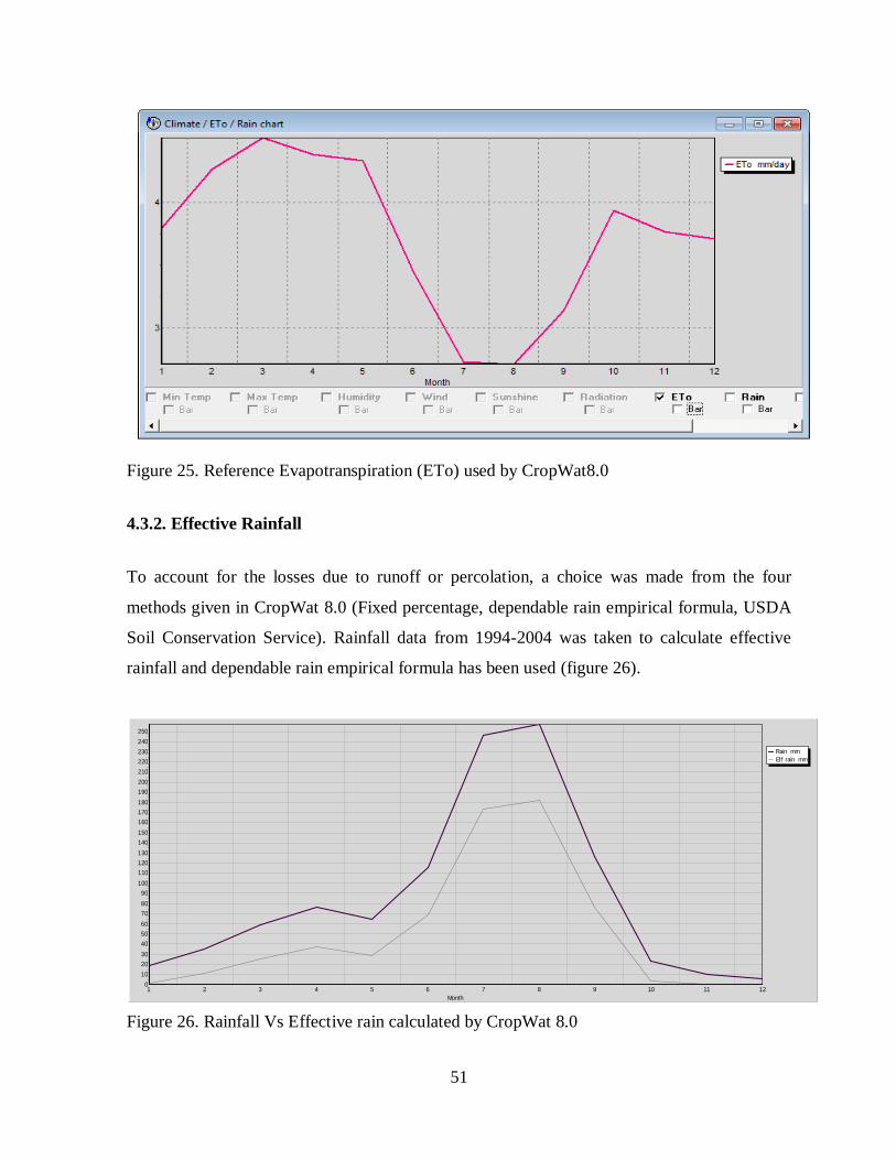
Figure 25. Reference Evapotranspiration (ETo) used by CropWat8.0 ................................... 51
Figure 26. Rainfall Vs Effective rain calculated by CropWat 8.0 .......................................... 51
XII
LIST OF TABELS IN THE APPENDIX Appendix I - 1. Effective rainfall for Holetta watershed ........................................................ 68
Appendix I - 2. Summary of crop water requirement for Potato ............................................ 71
Appendix I - 3. Summary of crop water requirement for Cabbage ......................................... 72
Appendix I - 4. Summary of crop water requirement for Tomato .......................................... 72
Appendix I - 5. Summary of crop water requirement for Barely ............................................ 73
Appendix I - 6. Monthly rainfalls in Holetta watershed (1994 - 2004) ................................... 74
Appendix I - 7. Yearly evapotranspiration calculation for Holetta catchment (1994 - 2004) .. 75
LIST OF FIGURES IN THE APPENDIX
Appendix II - 1. Summary of crop data for Potato ................................................................ 69
Appendix II - 2. Summary of crop data for Cabbage ............................................................ 69
Appendix II - 3. Summary of crop data for Tomato ............................................................. 70
Appendix II - 4. Summary of crop data for Apple ................................................................ 70
Appendix II - 5. Summary of crop data for Barely ............................................................... 71
Appendix II - 6. Holetta River diversion points .................................................................... 82
Appendix II - 7. Irrigated lands in the study area.................................................................. 83
XIII
ABSTRACT The hydrology of Holetta River and its seasonal variability is not fully studied. In addition to
this, due to scarcity of the available surface water and increase in water demand for
irrigation, the major users of the river are facing a challenge to allocate the available water.
Therefore, the aim of this research was to investigate the water availability of Holetta River
and to study the water management in the catchment using Geographical Information Systems
(GIS) tool, statistical methods, and hydrological model. The rainfall runoff process of the
catchment was modeled by Soil and Water Assessment Tool (SWAT). According to SWAT
classification, the watershed was divided in to 6 subbasins and 33 hydrological response units
(HRUs). The only gauged subbasin in the catchment was subbasin one that is found in the
upper part of the area. Therefore, sensitivity analysis, calibration, and validation of the model
was performed at subbasin one and then the calibrated model was used to estimate runoff at
the ungauged part of the catchment. The performance of SWAT model was evaluated by using
statistical (coefficient of determination [R2], Nash-Sutcliffe Efficiency Coefficient [NSE] and
Index of Volumetric Fit [IVF]) and graphical methods. The result showed that R2, NSE, and
IVF were 0.85, 0.84 and 102.8 respectively for monthly calibration and 0.73, 0.67 and 108.9
respectively for monthly validation. These indicated that SWAT model performed well for
simulation of the hydrology of the watershed. After modeling the rainfall runoff relation and
studying the availability of water at the Holetta River, the water demand of the area was
assessed. The survey form was used to identify information, which includes the number of
Holetta River consumers, major crops grown by irrigation and the total area coverage.
CropWat model was used to calculate the irrigation water requirement for major crops.
Based on the result of CropWat model and survey analysis, the irrigation water demand for
the three major users of Holetta River was calculated. The total water demand of all three
major users was 0.313, 0.583, 1.004, 0.873 and 0.341 MCM from January to May
respectively. The available river flow from January to May was taken from the result of SWAT
simulation at subbasins 2,3,4 and 5. The average flow was 0.749, 0.419, 0.829, 0.623 and
0.471 MCM from January to May respectively. From the five months, the demand and the
supply showed a gap during February, March and April. This indicated that there is shortage
of supply during these months with 0.59 MCM. Therefore, in order to solve this problem
XIV
alternative source of water supply should be studied and integrated water management
system should be implemented.
Keywords: runoff estimation, Holetta River, Awash basin, Ethiopia, hydrological modeling
1
1. INTRODUCTION
1.1. Background and Justification
Ethiopia is endowed with a huge surface and ground water resources. Many perennial and
annual rivers exist in the country. A number of lakes, dams, and reservoirs are also exists in
various parts of Ethiopia. Ethiopia has 12 river basins and the estimated total mean annual
flow from all the 12 river basins is 122 billion cubic meters (BMC )( see table 1).
Table 1. Ethiopian River basin's runoff and ground water potential (Awulachew et al., 2007)
River Basin Area (Km2) Runoff (BMC)
Estimated ground
water potential
(BMC)
Tekeze 82,350 8.2 0.2
Abbay 199,812 54.8 1.8
Baro-Akobo 75,912 23.6 0.28
Omo-Ghibe 79,000 16.6 0.42
Rift Valley 52,739 5.6 0.1
Mereb 5,900 0.65 0.05
Afar /Denakil 74,002 0.86 -
Awash 112,696 4.9 0.14
Aysha 2,223 - -
Ogaden 77,121 - -
Wabi-Shebelle 202,697 3.16 0.07
Genale-Dawa 171,042 5.88 0.14
Total 1,135,494 124.25 2.86
Holetta River is one of the rivers found in the upper part of Awash basin and facing
challenges of runoff variability and scarcity of water availability during the dry season. The
catchment has fertile soils (loam) and a high potential for water resource development.
However, development in the catchment is limited to a few hundred hectares of irrigation and
2
a small milling plant due to a very high seasonal variation of water availability. Farmers in
this area depend exclusively on rainfed agriculture and most crops grown in the main rainy
season (Kramer, 2000). The Holetta River is the main source of surface water in the study
area and it is a perennial river having three major users. These are Holetta Agricultural
Research Center (HARC), Tesdey Farm, and Village Farmers. Holetta Agricultural Research
Center is founded in 1963 and it is one of the potential consumers of Holetta River. In early
time, the HARC uses the Holetta River only for fruits and horticulture, but starting from 2011,
HARC is improving the facility of irrigation in the center to expand the irrigation coverage.
Tsedey Farm is a private company, which use Holetta River for irrigation purpose. They
mostly produce potato and vegetables like cabbage. The other major users of Holetta River
are the village farmers. These farmers use the river for traditional irrigation purposes. The
total area of irrigated farm by each farmer is about 0.25 hectares. The major products of the
farmers are vegetables and crops like potato, cabbage, and tomato. In addition to increasing
water demand in the area, there is no facility to store the water in the rainy season for future
use in the dry season. Therefore, the competition for water is increasing due to scarcity of
water and increasing pressure by expanding populations and increasing irrigation. In order to
alleviate this challenge, integrated water resources management, and effective water
allocation system is essential. Therefore, the aim of this research was to investigate the water
availability of Holetta River and to study the water management in the catchment using GIS
tool, statistical methods and hydrological model.
1.2. Problem Statement
With the risk of water shortages around the world becoming more and more of an issue, water
has become the fuel of certain conflicts in many regions around the world. Conflict due to
water sources are becoming usual in the world's future as the misuse of water resources
continues among countries that share the same water source. The rapid population increase
has greatly affected the amount of water readily available to many people. Many parts of
Ethiopia share one water resource for the use of their populations. A large percentage of these
populations are very dependent on the weather to provide proper irrigation to the agricultural
industry, since water resources are so scarce. Conflicts may rise from unequal distribution of
3
water supplies amongst neighboring users. With the growing demand for water resources,
conflicts seem almost inevitable, especially with poor management of resources and
inadequate conflict resolution mechanisms.
Holetta River is one of the rivers that face conflict between users. The competition for water
between the major users of Holetta River is increasing due to socio-economic development
and population growth in the catchment. Furthermore, the hydrology of Holetta River is not
fully assessed and studies investigating the variability and availability of water at Holetta
River are scarce. In addition to this, due to scarcity of the available surface water and increase
in water demand for irrigation, the major users of the river are facing a challenge to allocate
the available water. Furthermore, there is no rules and regulation to use the river properly and
to manage the watershed. Even if there is an irrigation committee of users, it is not well
established. Due to all the above reasons, the competing users start to face conflicts when
allocating the available water. With growing demands on limited water resources, effective
allocation and management of stream flow and reservoir storage have become increasingly
important. Therefore, this research mainly focuses on studying the hydrology of the Holetta
River and assessing the water management in the catchment.
1.3. Research Questions
What is the relationship between rainfall and runoff in the catchment? How much water is available in the Holetta River? How much is the water demand in the catchment? Is there a gap between the available river water supply and demand in the
catchment?
1.4. Objectives
General Objective
To study the hydrology of the Holetta River and to assess the water management
in the catchment
4
The specific objectives are to
model rainfall runoff relationship process of the catchment,
investigate the seasonal variability of runoff and water availability in the
catchment,
study the water demand in the catchment, and to quantify the gap between the
available river water supply and demand in the catchment.
1.5. Significance of the Study
As it is indicated earlier, studies investigating the variability and availability of water at
Holetta River are scarce. Furthermore, there is always a conflict between users during the dry
season. In order to have a proper river water management, identification of available water
and water demand is essential. Therefore, the result of this study can be an input for planning
and design of river management system in the area. In addition to this, it will give preliminary
information to develop water allocation system in the catchment.
1.6. Structure of the Thesis
This research paper is organized into five chapters. The first chapter deals with background,
statement of the problem, objectives and significance of the study. The second chapter
reviews related literature. The third chapter presents description of the study area and research
methodology. The fourth chapter explains the results and discussions of this research. The last
chapter presents the conclusions and recommendations of the study.
5
2. LITERATURE REVIEW
2.1. Global Water Management and Allocation Issues
Integrated Water Resource Management is a way of analyzing the change in demand and
operation of water institutions that evaluates a variety of supply side and demand side
management measures to determine the optimal way of providing water services. Demand
side management includes any measure or initiative that will result in the reduction in the
expected water usage or water demand. Supply side management includes any measure or
initiative that will increase the capacity of a water resource or water supply system to supply
water (Buyelwa, 2004).
The growing pressure on the world‘s fresh water resources is enforced by population growth
that leads to conflicts between demands for different purposes. The main concern on water
use is the conflict between the environment and other purposes like hydropower, irrigation for
agriculture and domestic, and industry water supply, where total flows diverted without
releasing water for ecological conservation. Consequently, some of the common problems
related to water faced by many countries are shortage, quality deterioration and flood impacts.
Hence, utilization of integrated water resources management in a single system, which built
up by river basin, is an optimum way to handle the question of water (Tessema, 2011).
There are several problems concerning water allocation and management, some of these are
Variability in rainfall, fluctuations in temperature and other meteorological
conditions greatly affect the variation in the magnitude and timing of hydrologic
events such as the distribution of stream flow.
Water demand driven by the rapid increase of population and increasing demand
for agricultural irrigation. This quick rate of growth brings severe consequences
that result from high stresses on water resources and their unprecedented impacts
on socio-economic development.
Water scarcity is also one of the problems in the river basins. The major reasons are
high water demand from population growth, degraded water quality and pollution
6
of surface and groundwater sources, and the loss of potential sources of fresh water
supply due to old and unsustainable water management practices.
Conflicts often arise when different water users of the river compete for limited
water supply (Lizhong, 2005).
2.2. Hydrological Models
A hydrological model is a simplified representation of a real-world system, and consists of a
set of simultaneous equations or a logical set of operations contained within a computer
program. Models have parameters, which are numerical measures of a property or
characteristics that are constant under specified conditions. Computer modeling offers a
methodology to investigate hydrological processes and make predictions on what the flow
might be in a river given a certain amount of rainfall. There are different types of models,
with different amounts of complexity, but all are a simplification of reality and aim to either
make a prediction or improve our understanding of biophysical processes (Davie, 2008).
Figure 1 showed different types of models.
Figure 1. Hydrological model classifications (Chow et al., 1988)
Hydological Models
Stochastic
Space Independent
Space Correlated
Deterministic
distributed model
lumped model
7
For this study, SWAT model was selected because of the following character and these
characters help to represent the catchment accurately,
It is physically based distributed model
Was capable of operating on a watershed scale with several subbasins
Allowed topographical, land use and soil differences
Was capable of simulating several management practices
Could simulate long periods of time
2.3. Description of SWAT Model
Soil and Water Assessment Tool (SWAT) is a river basin, or watershed, scale model
developed by Dr.Jeff Arnold for the US department of Agriculture (USDA) - Agricultural
Research Service (ARS) (Neitsch et al., 2005). Soil and Water Assessment Tool use to predict
the impact of land management practices on water, sediment, and agricultural chemical yields
in large, complex watersheds with varying soils, land use, and management conditions over
long periods. Soil and Water Assessment Tool is physically based distributed model requiring
specific information about soil, topography, weather, and land management practices within
the watershed. The physical processed associated with water movement, sediment movement,
crop growth and nutrient cycling directly modeled by SWAT using this input data (Arnold et
al., 1998). For modeling purposes, the watershed divided into a number of sub watersheds or
subbasins. Input information for each subbasin is organized into the following categories:
climate, hydrological response units (HRUs); ponds/wetlands; groundwater; and the main
channel or reach.
Simulation of the hydrology of a watershed can be separated into two major divisions. The
first division is the land phase of the hydrologic cycle. The land phase of the hydrologic cycle
controls the amount of water, sediment, nutrient, and pesticide loadings to the main channel in
each subbasin. The second division is the water or routing phase of the hydrologic cycle,
which can be defined as the movement of water, sediments, etc. through the channel network
of the watershed to the outlet (Neitsch et al., 2005).
8
2.3.1. Land Phase of the Hydrologic Cycle
The hydrologic cycle as simulated by SWAT is based on the water balance equation:
t
igwseepasurfdayt QWEQRSWSW
10
................ equation 1
Where, SWt is the final soil water content (mm H2O),
SW0 is the initial soil water content on day i (mm H2O),
t is the time (days),
Rday is the amount of precipitation on day i (mm H2O),
Qsurf is the amount of surface runoff on day i (mm H2O),
Ea is the amount of evapotranspiration on day i (mm H2O),
Wseep is the amount of water entering the vadose zone from the soil profile on day i
(mm H2O),
Qgw is the amount of return flow on day i (mm H2O).
The subdivision of watershed enables the model to reflect differences in evapotranspiration
for various crops and soils. Runoff is predicted separately for each HRU and it routed to
obtain the total runoff for the watershed. This increases accuracy and gives a much better
physical description of the water balance.
2.3.1.1. Climate
The climate of a watershed provides the moisture and energy inputs that control the water
balance and determine the relative importance of the different component of the hydrologic
cycle. The climatic variables required by SWAT consist of daily precipitation, maximum or
minimum air temperature, solar radiation, wind speed, and relative humidity. The model
allows values for daily precipitation, maximum/minimum air temperatures, solar radiation,
wind speed, and relative humidity to be an input from records of observed data or generated
during the simulation (Neitsch et al., 2005).
9
2.3.1.2. Hydrology
As precipitation descends, it may be intercepted and held in the vegetation canopy or fall to
the soil surface. Water on the soil surface will infiltrate into the soil profile or flow overland
as runoff. Runoff moves relatively quickly toward a stream channel and contributes to short-
term stream response. Infiltrated water may be held in the soil and later evapotranspired or it
may slowly make its way to the surface water system via underground paths.
Potential Evapotranspiration
Potential Evapotranspiration is the rate at which evapotranspiration would occur from a large
area uniformly covered with growing vegetation which has access to an unlimited supply of soil
water content. The model offers three methods for estimating potential evapotranspiration.
These are Hargreaves (Hargreaves et al., 1985), Priestley-Taylor (Priestley and Taylor, 1972),
and Penman-Monteith (Monteith, 1965). The three PET methods included in SWAT vary
based on the amount of required inputs. The Penman-Monteith method requires solar
radiation, air temperature, relative humidity, and wind speed. Priestley-Taylor method
requires solar radiation, air temperature, and relative humidity. The Hargreaves method
requires air temperature only. In this study, Penman-Monteith method was used. The Penman-
Monteith equation combines components that account energy needed to sustain evaporation,
the strength of the mechanism required to remove the water vapor, aerodynamic and surface
resistance terms. The Penman-Monteith equation is:
a
c
azozpairnet
rr
reeCGHE
1*
/***
................... equation 2
Where: λ is latent heat flux density (MJ/m2day)
E is depth rate evaporation (mm/day)
Δ is slope of saturation vapor pressure – temperature curve, de/dT (kPa/°C)
10
Hnet is net radiation (MJ/ m2day)
G is heat flux density to the ground (MJ/ m2day)
ρair is air density (kg / m3)
Cp is specific heat at constant pressure (MJ/kg.oC)
ez is water vapor pressure of air height z (kpa)
γ is psychometric constant (kpa /oC)
rc is pant canopy resistant (s/m)
ra is diffusion resistance of the air layer (aerodynamic resistance) (s/m)
Surface Runoff
Surface runoff, or overland flow, is flow that occurs along a sloping surface. Surface runoff
occurs whenever the rate of water application to the ground surface exceeds the rate of
infiltration. Using daily or sub daily rainfall amounts, SWAT simulates surface runoff
volumes and peak runoff rates for each HRU. Soil and Water Assessment Tool computes
surface runoff by using the modified soil conservation service (SCS) curve number method
(USDA - SCS, 1972) or the Green & Ampt infiltration method (Green and Ampt, 1911). In
the curve number method, the curve number varies non-linearly with the moisture content of
the soil. The curve number drops as the soil approaches the wilting point and increases to near
100 as the soil approaches saturation. The Green & Ampt method requires sub daily
precipitation data and calculates infiltration as a function of the wetting front metric potential
and effective hydraulic conductivity. Water that does not infiltrate becomes surface runoff.
The SWAT model includes a provision for estimating runoff from frozen soil where a soil is
defined as frozen if the temperature in the first soil layer is less than 0°C. In this study,
modified SCS curve number method was used.
11
The SCS curve number equation is (USDA - SCS, 1972):
SIR
IRQ
aday
adaysurf
2
............................... equation 3
Where, Qsurf is the accumulated runoff or rainfall excess (mm H2O),
Rday is the rainfall depth for the day (mm H2O),
Ia = is the initial abstractions prior to runoff (mm H2O),
S is the retention parameter (mm H2O).
The retention parameter varied especially due to changes in soils, land use, management, and
slope and temporally due to changes in soil water content. The retention parameter is defined
as:
1010004.25
CNS ..................... equation 4
Where, CN is the curve number for the day.
The Initial abstractions, Ia is commonly approximated as 0.2S and then the equation 3
becomes
SR
SRQ
day
daysurf 8.0
2.0 2
.................... equation 5
Runoff will only occur when Rday > Ia.
The peak runoff rate is the maximum runoff flow rate that occurs with a given rainfall event.
The peak runoff rate is an indicator of the erosive power of a storm and used to predict
sediment loss. Soil and Water Assessment Tool calculates the peak runoff rate with a
modified rational method. The rational method is based on the assumption that if a rainfall of
intensity i begins at time t = zero and continuous indefinitely, the rate of runoff will be
increase until the time of concentration, t = t conc, when the entire subbasin area is contributing
to flow at the outlet.
12
The rational formula is:
6.3** AreaiCq peak
...................... equation 6
Where, qpeak is the peak runoff rate (m3/s),
C is the runoff coefficient,
i is the rainfall intensity (mm/hr),
Area is the subbasin area (km2),
3.6 is a unit conversion factor (Neitsch et al., 2005).
2.3.2. Routing Phase of the Hydrologic Cycle
Once SWAT determines the loadings of water, sediment, nutrients, and pesticides to the main
channel, the loadings are routed through the stream network of the watershed using a
command structure. In addition to keeping track of mass flow in the channel, SWAT models
the transformation of chemicals in the stream and streambed (Neitsch et al., 2005).
2.4. Description of CROPWAT Model
CropWat is a decision support system developed by the Land and Water Development
Division of Food and Agriculture Organization (FAO) for planning and management of
irrigation. CropWat is a practical tool to carry out standard calculations for reference
evapotranspiration, crop water requirements, and crop irrigation requirements, and more
specifically the design and management of irrigation schemes. For this study, CropWat 8.0
was used. CropWat 8.0 is a computer programme for the calculation of crop water
requirements and irrigation requirements from existing or new climatic and crop data.
Furthermore, the program allows the development of irrigation schedules for different
management conditions and the calculation of scheme water supply for varying crop patterns.
In CropWat 8.0, the calculation of crop water requirements is carried out per decade.
13
2.4.1. Crop Water Requirement
The amount of water required to compensate the evapotranspiration loss from the cropped
field is defined as crop water requirement. Although the values for crop evapotranspiration
and crop water requirement are identical, crop water requirement refers to the amount of
water that needs to be supplied, while crop evapotranspiration refers to the amount of water
that is lost through evapotranspiration. The irrigation water requirement represents the
difference between the crop water requirement and effective precipitation. The irrigation
water requirement also includes additional water for leaching of salts and water to compensate
for non-uniformity of water application. For the calculations of the Crop Water Requirements
(CWR), the crop coefficient approach is used (Allen et al., 1998).
2.4.2. Crop Coefficient Approach
Crop evapotranspiration can be calculated from climatic data and by integrating directly the
crop resistance, albedo and air resistance factors in the FAO Penman-Monteith approach. As
there is still a considerable lack of information for different crops, the Penman-Monteith
method is used for the estimation of the standard reference crop to determine its
evapotranspiration rate, i.e., reference evapotranspiration (ETo). Experimentally determined
ratios of ETc/ETo, called Crop coefficient (Kc), are used to relate crop evapotranspiration
under standard conditions (ETc) to ETo. This is known as the crop coefficient approach.
ETc = Kc * ETo ...................... equation 7
Radiation, air Temperature, Humidity and Wind speed are all incorporated into the ETo
estimate. Therefore, ETo represents an index of climatic demand, while Kc varies
predominately with the specific crop characteristics and only to a limited extent with climate
and soil evaporation. This enables the transfer of standard values for Kc between locations
and between climates. This has been a primary reason for the global acceptance and
usefulness of the crop coefficient approach and the Kc factors developed in past studies. The
reference ETo is defined and calculated using the FAO Penman-Monteith equation. The crop
14
coefficient, Kc represents an integration of the effects of four primary characteristics that
distinguish the crop from reference grass. These characteristics are crop height, Albedo of the
crop soil surface, canopy resistance, and evaporation from soil, especially exposed soil (Allen
et al., 1998).
2.4.3. Effective Rainfall
For agricultural production, effective rainfall refers to the portion of rainfall that can
effectively be used by plants. This shows not all rain is available to the crops as some is lost
through runoff and deep percolation. How much water actually infiltrates the soil depends on
soil type, slope, crop canopy, storm intensity, and the initial soils water content. During the
rainy season in tropical and some semi-tropical regions, a great part of the crop's water needs
are covered by rainfall, while during the dry season, the major supply of water should come
from irrigation. How much water is coming from rainfall and how much water should be
covered by irrigation is, unfortunately, difficult to predict as rainfall varies greatly from
season to season. In order to estimate the rainfall deficit for irrigation water requirements, a
statistical analysis needs to be made from long-term rainfall records (Allen et al., 1998).
2.5. Previous Study in the Area 2.5.1. Design of a community based Dam in Holetta, Ethiopia
The purpose of this work was to design a small dam in the Holetta area, which can be
constructed economically using local labor skills. The study proposed two dam sites in which
both found in the Mintile River and have a catchment area of 38.06km² and 63.72km². The
overall annual water demand for the irrigation area was about 9 to 11 million cubic meters
(MCM) for the years 1985-1993. In this estimation, the water demand for drinking water was
included. The drinking water demand was found to be 1,700m³/day, which means a yearly
demand of 620,500m³/year. The annual water demand was 5.6 MCM/year. According to
Ethiopian consultants, a rough estimation value for water irrigation per hectare of land per
year was 10,000m³/ha/year, with an irrigation area of 680ha this was an annual water demand
of 6.8MCM/year (Kramer, 2000).
15
2.5.2. Simulation and Optimization for Irrigation and Crop planning
In this work, simulation and optimization models were assembled for the optimization of
irrigation systems and their operation. The simulation model CropWat was used for
estimation of the crop water requirement, time, and depth. The study area encompasses three
command areas that are Holetta Research Center, farmers and Tsedey State Farm, and five
different types of crops, i.e. potato, tomato, apple, peach, and winter wheat. The simulation
results of the CropWat model illustrated that crop water requirement for apple was highest
(993 mm), followed by peach (908 mm), tomato (470 mm), potato (443 mm) and wheat
(294 mm). The study reveals that fruit crops have more crop water requirements than cereals
(Darshana et al., 2011).
16
3. MATERIALS AND METHODS 3.1. Description of Study Area The study was conducted at Holetta catchment, which is located in the upper part of Awash
River basin, Ethiopia. The study area lies at an altitude of 2069 - 3378 meters above sea level
and located at a latitude range of 8056'N to 9013'N and longitude range of 38024'E to 38036'
E. It is a catchment with drainage area of 403.47 km2. According to the national census
conducted in 1994, the population of the town for that year was 16,785, consisting mainly of
Oromo people. However, according to census carried out by the municipality of the town in
1998, the estimated population is 29,421(Kramer, 2000). The loamy soil of the study area is
the main cause of erosion in the rainy season. The annual rainfall of the study area ranges
between 818-1226 mm. The climate of the study area is described with the air temperature
ranging from 60C to 230C with the mean of 14 0C.
The town of Holetta is the major settlement in the catchment of the Holetta River, which is
the capital of the Wolmera Genet area and 45 km in the west direction from Addis Ababa. The
total length of streams in the watershed is about 45.51 km. About 5km north of Holetta town
is the conjunction of the Holetta and the Mintile River, which originates in the mountains. At
the end, the Holetta River will join with Awash River at Ilu Woreda. In addition to HARC and
Tsedey Farm, four kebele's in the downstream use the river for irrigation which was
considered as the major users of the river. These are Medi Gudina, Dewana Lafto, Tulu Wato
Dalecha and Hamus Gebeya. Farmers in these kebeles produce cereals under rainfed
agriculture from June to November for subsistence. Potatoes and tomatoes are the dominant
irrigated horticultural crops, although several other crops are also cultivated.
17
Figure 2. Location of Holetta catchment
3.1.1 .Topography The altitude of the study area ranges from 2069 to 3378 meters (m) above sea level (a.s.l) with
a mean of 2496m a.s.l. According to Food and Agricultural Organization (FAO/UNESCO,
1974) slope classification, most slope in watershed (54.01%) are flat to gently undulating
with a dominant slopes ranging between 0-8%, 41.9% of the area is rolling to hilly with a
dominant slopes ranging between 8-30% and only 4.09% are steeply dissected to mountainous
with dominant slopes over 30%. Figure 3 showed the graphical distribution of these slopes.
18
Figure 3. Slop classification map of study area
3.1.2. Climate
The central and most of the eastern part of the country have two rainy periods and one dry
period. These seasons are known locally as the main Kiremt rains from June to September,
small Belg rains, from February to May, and dry Bega season from October to January. The
annual rainfall of the study area ranges between 818-1226 mm, with a bimodal pattern of
main rainy season during June to September and short rain
y season during January to May. There is relatively intensive rainfall during June to August
with the highest mean monthly rainfall recorded in July - 243 mm. The months with the
lowest rainfall are November and December.
19
3.1.3. Land use/ Land cover
The major land use and land cover types of the watershed are agriculture land, forest,
pastureland, settlement, and water bodies. Forests and woodlands occur on the better-drained
soils of mountains and sides of the valleys, and grasslands occupy areas of heavy clay soil of
the valley bottom.
The forest coverage of the Welmera Wereda is 8,917 ha (8.5%) of the total area of the
Wereda. This forest coverage is high due to the existence of Suba state forest, Managasha
Church and Monastery and Finfinnee area Forest Enterprise plantation Forest. There are some
remnants of indigenous tree species such as Podocarpus gracilior, Juniperus procera, Olea
Africana, Croton macrostachyus and Acacia spp in the watershed. The dominant cultivated
Eucalyptus species are Eucalyptus globules and Eucalyptus camaldulensis. The cultivated
Eucalyptus mostly used for construction and as an energy source in the wereda. Nowadays it
has become one of the cash crops in the wereda and a means of income source. This pushes
the farmers to unplanned harvesting of the plantation forest thereby reducing land cover and
having an effect on soil erosion on the area (Ayele, 2011).
3.1.4. Soil Classification
The soil type in the study area is classified as vertisols, cambisols and nitisols. However, the
dominant are vertisols and nitisols. Vertisols occur on smooth plains and on rolling
topography of the plateau. They are characterized by their high clay content and have in
general a good natural fertility. Due to clay mineralogy they are very hard and crack when
dry; sticky and plastic when wet. Nitisoil generally occur on steeper hill slopes of the plateau
and in the upper parts of the Holetta catchment. These soils contain more than 35% clay. The
high clay content of Nitisoils result in somewhat better chemical and physical properties than
other tropical soils related to the soil depth, stable structure and high water holding capacity
permeability (Kramer, 2000).
20
3.2. Data Collection
All meteorological data (rainfall, temperature, relative humidity, wind speed, and sunshine
hour) were collected from National Meteorology Agency and Holetta Research Center. Flow
data and GIS data (topographic, land use/cover data and map, soil map) were collected from
Ministry of Water and Energy. Primary data of crop type and area coverage were collected
from major water users of Holetta River (Holetta Agricultural Research Center, Tsedey Farm,
and Farmers). The method of data collection was documents, field survey, and questionnaire.
The survey form was used to collect crop type, area coverage and water use data from the
three users of Holetta River and Agricultural office. Then, the sample size of households was
determined by the following formula (Cochran, 1977).
1)/)((11
/)(22
22
dpqZN
dpqZn ...................... equation 8
Where, n= is the desired sample size
N = the number of sample size when the population is less than 1000
Z = 95% confidence limit i.e. 1.96
P = 0.1(proportion of the population to be included in the sample i.e. 10%)
q =1-P =1- 0.1, =0.9
N = total number of population
d = margin of error or degree of accuracy desired (0.05)
Based on the above formula 100 respondents were selected using random sampling
techniques.
21
3.3. SWAT Model Input
Soil and Water Assessment Tool required the following data to be defined for the physical
watershed representation, topography data (Digital Elevation Model), climate (daily
measured and monthly statistical weather data), flow data, soil and land use data (maps and
physical parameters).
3.3.1. Digital Elevation Model Data
The Digital Elevation Model (DEM) of Awash basin was taken from Ministry of Water and
Energy GIS department. Then, a 90m resolution DEM was used in SWAT model to delineate
the Holetta catchment and to analyze the drainage patterns of the land surface terrain.
Figure 4. Digital elevation model (90m) of Awash basin
22
3.3.2. Land Use Map The land use map of Awash basin clipped and dissolved into Holetta River catchment. Then,
the clipped land use map was used for SWAT land use reclassification. According to SWAT
land use classification, the catchment has five categories (figure 5). These are, Agricultural
Land- Row Crops (AGRR) with an area of 13.54%, Agricultural Land -Close-Grown (AGRC)
- 0.17%, Wetlands-Mixed (WETL) - 0.14%, Forest -Deciduous (FRSD) - 57.26% and Forest-
Mixed (FRST) - 28.9%.
Figure 5. Land use classification of SWAT model for Holetta watershed
23
3.3.3. Soil Map The soil map of Awash basin clipped and dissolved in to Holetta River catchment. Then, the
clipped soil map was used for SWAT soil reclassification. Based on SWAT reclassification,
the catchment has four soil categories (figure 6). These are Chromic Luvisols (Chluvisols)
with an area of 33.26%, Humic Nitisols (Huntisols) - 56.57%, Vertic Cambisols (Vtcambisol)
-1.71% and Eutric Vertisols (Euvertisols) - 8.27%. Based on their texture, Vtcambisol and
Euvertisol classified as clay whereas Chluvisols and Huntisols classified as loam (Belete et
al., 2012).
Figure 6. Soil classification of SWAT model for Holetta watershed
24
3.3.4. Meteorological Data
One of the meteorological stations (Holetta) found inside the catchment. The other
meteorological stations, which were found outside the catchment, are Addis Alem, Kimoye
and Welenkomi. The meteorological data measured from Holetta station are Rainfall,
Maximum and Minimum temperature, Relative humidity, Wind speed, and Sunshine hour. All
the other meteorological stations were used only for rainfall data. The consistency,
homogeneity, and outlier test for the data was performed by using Excel software and
XLSTAT software. The percentage of miss data for rainfall is 14% at Addis Alem station,
13% at Kimoye station, 1% at Holetta station, and 18% at Welenkomi station. Therefore,
missing data are filled from observations at the three nearby stations by using the normal ratio
method. The normal ratio method is a better method than the arithmetic mean method and is
usually applied when the normal annual precipitation at the site with the missing record
differs by more than 10% of the normal annual precipitation at the other sites where the
concurrent data are available. The location of the four meteorological stations was shown in
figure 7.
Figure 7. Location of rainfall stations for the study area
25
Table 2. Information of climate and hydrology stations
No Station Record Period
Coordinate Elevation Data
collected XPR YPR
1 Addis Alem 1994 -2004 475810.95 981592.52 2100 Rainfall
2 Holetta 1994 -2004 447252.34 1003731.64 2395 Climate
and Flow data
3 Kimoye 1994 -2004 423058.00 998462.26 2260 Rainfall
4 Welenkomi 1994 -2004 423058.00 996021.93 2160 Rainfall
The climate data obtained from Holetta station showed that the air temperature in the area
ranges from 60C to 230C. The mean maximum temperature was 250C. Based on
meteorological data from 1994-2004, the mean monthly relative humidity value varied from
45 to 85% (figure 8).
Figure 8. Average Rainfall, Temperature and Relative humidity of Holetta watershed (1994 -
2004)
0.00
5.00
10.00
15.00
20.00
25.00
30.00
0.00
50.00
100.00
150.00
200.00
250.00
300.00
Jan Feb Mar Apr May Jun Jul Aug Sep Oct Nov Dec
Max
. & M
in. T
empe
ratu
re (
oc)
Rai
nfal
l (m
m) ,
H
umid
ity (%
) Average Monthly Rainfall(mm)
Average Monthly Relative Humidity(%)Minimum Temperature(oc)
Maximum Temperature(oc)
26
3.3.5. Flow Data
The Holetta River is a tributary of the larger Awash River, which joins it after travelling about
25km downstream of the gauging station. The Holetta River is the main source of surface
water in the study area. The River is gauged since 1975 and for this study, the 1994 - 2004
time series of the river discharge data was used. The daily flow data from gauging station was
used for sensitivity analysis, model calibration (1994 – 1999) and validation (2000-2004).
The average annual river flow at Holetta River was 44 MCM (figure 9). The flow was low
from January to May and it started to increase at June. The peak flow was 17 MCM, which
occurred in August, and the minimum flow was 0.524 MCM in February.
Figure 9. Average monthly flows at Holetta River (1994 -2004)
The rainfall runoff relation showed that there was a positive relation between rainfall and
surface runoff in the catchment (figure 10).
0
5
10
15
20
25
30
35
Jan Feb Mar Apr May Jun Jul Aug Sep Oct Nov Dec
Monthly Flow (MCM)19941995
1996
19971998
1999
20002001
2002
2003
2004Average Flow
27
Figure 10. Monthly rainfall runoff relations for Holetta subbasin (1994-2004)
3.4. SWAT Data Preparation and Model Setting
First new SWAT project was set up and saved, and then watershed delineation was
performed. In order to delineate the watershed, automatic watershed delineation was selected.
Then, the DEM was added and stream network was defined. Finally, the watershed outlet was
selected to delineate the basin. The next step in setting up a watershed simulation was to
divide the watershed into subbasins. The subbasins possess a geographical position in
watershed and they are spatially related to one another. In this study, the DEM of Awash
basin was used to delineate the watershed. Once the subbasin delineation completed, the user
has the option of modeling a single soil, land use and management scheme for each subbasin
or partitioning the subbasins into multiple hydrologic response units (HRUs). Hydrological
response units are portion of a subbasin that possesses unique land use, management and soil
attributes. A subbasin will contain at least one HRU, a tributary channel and a main channel
or reach. Hydrological response units are used in most SWAT runs because they simplify a
run by lumping all similar soil and land use areas into a single response unit and it will
increase the accuracy (Neitsch et al., 2004).
y = 0.426x - 3.614R² = 0.630
0.00
40.00
80.00
120.00
160.00
0.0 40.0 80.0 120.0 160.0 200.0 240.0 280.0Aver
age
Mon
thly
Run
off (
mm
)
Average Monthly Rainfall (mm)
Rainfall Runoff Relation
Series1
Linear (Series1)
28
After that land use/soil / slop definition and HRU definition was performed by using the land
use and soil map in combination with look up tables. By using these data, SWAT classified
the watershed. Then, writing input tables was continued by defining weather data. The first
step to proceed was defining the weather generator data. To define the weather generator data,
the user weather station was created through edit SWAT database section. Then, the weather
station parameters were fitted in the new station.
In order to prepare the station parameters, different software was used. These are
WGNmaker4.Xlsm, dew.exe and pcpSTAR.exe. WGNmaker 4.Xlsm was used to calculate
the weather station statistics needed to create user weather station files. The program dew.exe
was used to calculate the average daily dewpoint temperature per month using daily
temperature and humidity data. The program pcpSTAT.exe was used to calculate statistical
parameters of daily precipitation data used by weather generator of SWAT model (Stefan,
2003). Then, the arranged data was used by SWAT weather generator to fill in missing
information and to simulate weather data. To finalize the weather writing part, write all
section was selected and then all the watershed data was written and the model was made to
be ready to run.
Once we run the model with default parameter setting, the sensitivity analysis and calibration
was performed. The sensitivity analysis was performed by selecting the SWAT simulation,
subbasin, sensitivity parameters and observed data. The calibration can be performed in two
methods, auto calibration and manual calibration methods. In this study, manual calibration
was used. That was by changing the sensitive parameters manually until the simulation was
better fit with the observed data.
3.5. Sensitivity Analysis
Sensitivity analysis explores how changes in parameter values affect the overall change in the
output of the model. This can be done by using simple sensitivity analysis, where only one
parameter is changed or more complex arrangements that explore the relationships between
multiple parameters. Sensitivity analysis is important for a model to reduce the number of
29
model parameters for calibration and to examine the more sensitive parameters. Thus, a
sensitivity analysis for SWAT model was performed for the entire data (1994 -2004). Then,
the most sensitive parameters was identified and used for calibration of the model.
The Latin Hypercube - One-factor-At-a-Time (LH-OAT) sensitivity analysis method
combines the robustness of the Latin Hypercube sampling with the precision of One-factor-
At-a-Time (OAT) designs. The LH ensures the full range of all parameters has been sampled
and OAT assured that the changes in the output in each model run could be unambiguously
attributed to the input changed in such a simulation leading to a robust and efficient sensitivity
analysis method. The method is also efficient, as for m intervals in the LH method, a total of
m*(p+1) runs are required. Latin-Hypercube is a sophisticated way to perform random
sampling such as Monte-Carlo sampling to allow a robust analysis requiring not too many
runs. One-factor-At-a-Time design is an example of an integration of a local to a global
sensitivity method. As in local methods, each run has only one parameter changed, so the
changes in the output in each model run can be unambiguously attributed to the input
parameter changed ( VanGriensven, 2005).
3.6. Model Calibration and Validation
Model calibration is often important in hydrologic modeling studies, since uncertainty in
model predictions can be increased if models are not properly calibrated. Calibration is
changing of model parameters based on sensitivity results against observations to ensure the
same response over time. This involves comparing the model results, entered with the
recorded stream flows. In this process, model sensitive parameters varied until recorded flow
patterns are accurately simulated. Model validation involves re-running the model using input
data independent of data used in calibration keeping the calibrated parameters constant. For
this study, the calibration was carried out for six years (1994 - 1999) with one-year warm up
period and it was done based on the result of sensitivity analysis. Then, validation of SWAT
model was performed for the next five years (2000 -2004).
30
3.7. Model Evaluation
The SWAT model performance was evaluated by using statistical measures and graphical
methods of comparing simulated with observed data. Three methods for goodness-of-fit
measures of model predictions were used during the calibration and validation periods, these
numerical model performance measures are coefficient of determination [R2], the Nash-
Sutcliffe Efficiency Coefficient [NSE] and Index of Volumetric Fit [IVF].
The coefficient of determination (R2) is defined as the squared value of the coefficient of
correlation according to Bravais- Pearson. It is calculated as:
2
1
2
1
2
12
n
ii
n
ii
n
iii
PPOO
PPOOR
............. equation 9
Where, O is observed and P is predicted values.
The coefficient of determination (R2) expressed as the squared ratio between the covariance
and the multiplied standard deviations of the observed and predicted values. Therefore, it
estimates the combined dispersion against the single dispersion of the observed and predicted
series. The range of R2 lies between zero and one, which describes how much of the observed
dispersion is explained by the prediction. A value of zero means no correlation at all whereas
a value of one means that the dispersion of the prediction is equal to that of the observation
(Krause et al., 2005).
The Nash-Sutcliffe Efficiency Coefficient (NSE) is a normalized statistic that determines the
relative magnitude of the residual variance compared to the measured data variance (Nash and
Sutcliffe, 1970). Nash-Sutcliffe Efficiency indicates the degree of fitness of the observed and
simulated plots.
31
The Nash–Sutcliffe Efficiency Coefficient is used to assess the predictive power of
hydrological models. It is defined as:
n
ii
n
iii
OO
PONSE
1
21
2
1
............. equation 10
Where, O is observed and P is predicted values (Krause et al., 2005).
The Nash Sutcliffe Efficiency Coefficient (NSE) ranges between −∞ and 1.0 (1 inclusive),
with NSE = one being the optimal value. Values between 0.0 and 1.0 are generally viewed as
acceptable levels of performance, whereas values < 0.0 indicates that the mean observed value
is a better predictor than the simulated value, which indicates unacceptable performance.
Essentially, when the model efficiency is closer to one, the model is more accurate. General
performance rating for NSE for monthly time step is very good for 0.75 < NSE < 1.00, good
for 0.65 < NSE < 0.75, satisfactory for 0.60 < NSE < 0.70 and unsatisfactory for NSE< 0.5
(Moriasi et al., 2007).
The Index of Volumetric Fit, IVF is the ratio of total volume of Qp to the total volume of Q0,
and is given by,
n
io
n
ip
Q
QIVF
1
1 *100 ................ equation 11
Where, Q0 is observed flow and Qp is predicted flow
For the Index of Volumetric Fit IVF, the value of unity indicates a perfect volumetric match
of the observed flows with the estimated flows over a certain period, indicating water balance
(Birhanu, 2009).
32
3.8. Runoff Estimation
Runoff for ungauged catchments can be estimated by three regionalization method. The first
method is by establishing a regional model between catchment characteristics and model
parameters. The second method is Spatial Proximity; it simply transfers model parameters
from nearby catchments to ungauged catchments to allow for runoff simulation. The third
method is Area Ratio method; in this case, parameter sets of gauged catchments are
transferred to ungauged catchments by a simple area comparison.
3.9. CropWat Model Input
Calculations of the crop water requirements and irrigation requirements were carried out with
inputs of climatic, crop and soil data. The model required the following data for estimating
crop water requirements (CWR).
3.9.1. Climatic Data
In order to calculate the reference evapotranspiration, CropWat model use 11 years (1994 -
2004) of monthly maximum and minimum temperature, relative humidity, sunshine hour, and
wind speed data that was collected from Holetta station.
3.9.2. Rainfall Data
Effective rainfall was calculated based on 11 years (1994 -2004) monthly rainfall data
collected from Holetta station. The annual rainfall in the catchment ranges 818 -1226 mm.
The average maximum monthly rainfall is 243 mm, which occurred in July, and the minimum
is zero occurred in December.
33
3.9.3. Cropping Pattern Data
A Cropping pattern data includes planting date, crop coefficient data files (including Kc
values, stage days, root depth, depletion fraction) and the area planted (0-100% of the total
area).
A survey was carried out in the study area to assess the crops grown under irrigation. The
present cropping pattern data was assessed through field observations, interviews with
farmers, HARC, and Tsedey farm workers. Additional information was taken from
Agricultural office, kebele Administration and FAO-33 (Doorenbos and Kassam, 1986).
Essential information collected from the above sources includes:
Crop and crop variety
Planting date
Crop coefficient (Kc)
Field irrigation methods
Rooting depth
Allowable depletion levels
Critical depletion fraction (p)
Length of individual growth stages
The Crop module requires crop data over the different development stages, defined as follow:
Initial stage: it starts from planting date to approximately 10% ground cover.
Development stage: it runs from 10% ground cover to effective full cover.
Effective full cover for many crops occurs at the initiation of flowering.
Mid-season stage: it runs from effective full cover to the start of maturity. The
start of maturity is often indicated by the beginning of the ageing, yellowing, or
senescence of leaves, leaf drop, or the browning of fruit to the degree that the
crop evapotranspiration is reduced relative to the ETo.
Late season stage: it runs from the start of maturity to harvest or full senescence.
34
3.9.4. Soil Type Data
Soil type data includes total available soil moisture, maximum rooting depth, initial soil
moisture depletion (percentage of total available moisture), and maximum infiltration rate.
The above data of soil collected from the soil survey carried out at HARC and FAO-33
document (Doorenbos and Kassam, 1986).
35
4. RESULTS AND DISCUSSIONS
4.1. Hydrological Analysis
Watershed delineation and determination of HRUs were the first step in SWAT model
analysis. Then, weather station and all the necessary data were fitted. After setting and
running SWAT model, sensitivity analysis, calibration and validation was performed. In this
study, the calibration and validation was performed at subbasin one (see figure 12 and figure
15). A long term data was required for the analysis and the results are highly dependent on the
accuracy of the data.
4.1.1. Watershed Delineation and Determination of HRUs
Holetta River catchment delineated by SWAT model has six subbasins. Then, the subbasins
were divided into HRUs. The HRUs can be determined either by assigning only one HRU for
each subbasin considering the dominant soil/land use combinations, or by assigning multiple
HRUs for each subbasin considering the sensitivity of the hydrologic processes based on a
certain threshold values of soil/land use combinations. In this study, a multiple HRU
definition with a threshold value of 15% for land use, 20% for soil class, 5% for slope were
given and as a result, 33 HRUs were identified.
4.1.2. Sensitivity Analysis
Sensitivity analysis was performed for the entire period (1994-2004). About 270 iteration
have been done by SWAT sensitivity analysis for flow calibration with the output of 26
parameters were reported as sensitive in different degree of sensitivity for flow. Among these
26 parameters, eight of them have more effect on the simulated result when changed. Based
on the result of sensitivity analysis, table 3 showed the most sensitive parameters for the
watershed. Then, these parameters were used for calibration.
36
Table 3. Result of sensitivity analysis of flow at Holetta subbasin
Rank parameter Description Mean
1 Canmx Maximum canopy storage [mm] 0.18
2 Alpha_Bf Base flow alpha factor [days] 0.15
3 Revapmn Threshold water depth in the shallow aquifer
for "revap" [mm] 0.15
4 Gwqmn Threshold water depth in the shallow aquifer
for flow [mm] 0.06
5 Gw_Revap Groundwater "revap" coefficient 0.06
6 Esco Soil evaporation compensation factor 0.04
7 Cn2 Initial SCS CN II value 0.01
8 Sol_K Saturated hydraulic conductivity [mm/hr] 0.00
4.1.3. Model Calibration
After sensitivity analysis has been carried out, the calibration of SWAT model was done
manually. The calibration was carried out using the output of the sensitivity analysis of the
model and by changing the more sensitive parameter at a time while keeping of the rest of the
parameters constant. The analysis of simulated result and observed flow data comparison was
considered daily and monthly. The calibration was performed until the best-fit curve of
simulated versus measured flow was obtained.
The sensitive parameters were adjusted based on the allowable range until the best fitting
value was found. Table 4 showed the initial/default and finally adjusted parameter values.
37
Table 4. Initial and final adjusted value of calibrated flow parameters at Holetta subbasin
No parameter Default Range ( Upper &
Lower Limit )
Final Calibrated
Value
1 Canmx 0 0-10 10
2 Alpha_Bf 0.048 0-1 0.4
3 Revapmn 1 0 -1 0.01
4 Gwqmn 0 0-5000 70
5 Gw_Revap 0.02 0.02 -0.2 0.2
6 Esco 0 0-1 0.01
7 Cn2 72 ±50% +12%
8 Soil_K 18 0-2000 120
The SWAT model performance was evaluated by using statistical and graphical methods of
comparing simulated with observed data. The goodness-of-fit statistics was used in describing
the model’s performance relative to the observed data. These statistical measures were the
coefficient of determination (R2), Nash-Sutcliffe Efficiency Coefficient (NSE), and Index of
Volumetric Fit (IVF) between the observations and the final best simulations. Figure 11 and
12 showed the daily and monthly graphical performance evaluation of SWAT model during
calibration period respectively. Both the daily and monthly graphs implied that the model
simulation is best fitted with the observed flow measurement. During some years on daily
bases, it showed that the model does not exactly capture the peak values; this may be due to
inadequate gauging stations in the area. The catchment has only one gauging station and
according to World Meteorological Organization (WMO, 2008) standard, it failed to represent
the rainfall for the whole area. The WMO guide manual recommends that one rain gauge
station cover an area of 250Km2 for areas with similar terrain characteristics to the study area.
38
Figure 11. Observed and simulated hydrograph after daily calibration
Figure 12. Observed and simulated hydrograph after monthly calibration
The daily calibration result showed that the regression coefficient (R2) was 0.57; Nash-
Sutcliffe Efficiency Coefficient (NSE) was 0.55 and Index of Volumetric Fit (IVF) was
0.00
5.00
10.00
15.00
20.00
25.00
1/1/1995 1/1/1996 1/1/1997 1/1/1998 1/1/1999
Stre
am Fl
ow (m
3 /s)
Time(date/month/year)
Observed Flow
Simulated Flow
0.001.002.003.004.005.006.007.008.009.00
10.00
Jan-
95
May
-95
Sep-
95
Jan-
96
May
-96
Sep-
96
Jan-
97
May
-97
Sep-
97
Jan-
98
May
-98
Sep-
98
Jan-
99
May
-99
Sep-
99
Stre
am Fl
ow (m
3 /s)
Time
Observed Fow
Simulated Flow
39
102.62 %. In addition, based on monthly calibration the result showed that the regression
coefficient (R2) was 0.85; Nash-Sutcliffe Efficiency Coefficient was 0.84 and Index of
Volumetric Fit was 102.8% (figure 13). These indicated that the model performance was very
good and highly acceptable.
Figure 13. Scattered plot & correlation between simulated & observed monthly flow during
calibration
4.1.4. Model Validation
The validation process was performed by simply executing the model for the different period
using the previously calibrated input parameters. Figure 14 and figure 15 showed the daily
and monthly graphical performance evaluation of SWAT model during validation period
respectively. Both the daily and monthly graphs implied that the model simulation is best
fitted with the observed flow measurement.
y = 0.968x + 0.081R² = 0.853
0
2
4
6
8
10
0 2 4 6 8 10
Sim
ulat
ed D
isch
arge
(m3 /
s)
Observed Discharge Data (m3/s)
Simulated Flow
Linear (Simulated Flow)
40
Figure 14. Observed and simulated hydrograph during daily model validation
Figure 15. Observed and simulated hydrograph during monthly model validation
The three goodness-of-fit measures were also calculated for the validation period. The daily
calibration result showed that the regression coefficient (R2) was 0.44; Nash-Sutcliffe
Efficiency Coefficient (NSE) was 0.4 and Index of Volumetric Fit (IVF) was 108.9 %.
0.00
5.00
10.00
15.00
20.00
25.00
1/1/2000 1/1/2001 1/1/2002 1/1/2003 1/1/2004
Stre
am fl
ow (m
3 /s)
Time(date/month/year)
Observed Flow
Simulated Flow
0.00
1.00
2.00
3.00
4.00
5.00
6.00
7.00
8.00
Jan-
2000
May
-200
0
Sep-
2000
Jan-
2001
May
-200
1
Sep-
2001
Jan-
2002
May
-200
2
Sep-
2002
Jan-
2003
May
-200
3
Sep-
2003
Jan-
2004
May
-200
4
Sep-
2004
Stre
am Fl
ow (m
3 /s)
Time
Observed Flow
Simulated Flow
41
In addition, based on the result of monthly validation, the regression coefficient was 0.73;
Nash-Sutcliffe Efficiency Coefficient was 0.67 and Index of Volumetric fit was 108.9%
(figure 16). These results indicated that the model performance was good in the acceptable
limit.
Figure 16. Scattered plot & correlation between simulated & observed monthly flow during
validation
4.1.5. Runoff Estimation for Holetta Catchment
The Holetta catchment was divided into six subbasins. Only one of the subbasin was gauged
which is found in the upper part of the catchment. The calibration and validation of SWAT
model was performed at subbasin one. Then, regionalization approach was used to estimate
runoff for the ungauged subbasin's of the catchment.
In this study, Spatial Proximity method was used to estimate runoff at subbasins 2, 3, 4 and 5
where majority of the users located. Figure 17 and figure 18 showed the daily simulation
result of SWAT model. Figure 19 and figure 20 showed the monthly simulation result of
SWAT model at the subbasins. The mean flow (m3/s) at the subbasin 2, 3, 4 and 5 was shown
in table 5.
y = 0.933x + 0.148R² = 0.730
0
2
4
6
8
0 2 4 6 8
Sim
ulat
ed D
isch
arge
Dat
a (m
3 /s)
Observed Discharge Data (m3/s)
Simulated Flow
Linear (Simulated Flow)
46
Table 5. Summary of mean flow (m3/s) at the subbasins
Subbasin Mean daily flow (m3/s)
Mean monthly
flow (m3/s)
Mean annual flow (m3/s)
2 1.358 1.351 1.358
3 0.564 0.561 0.564
4 2.109 2.099 2.109
5 0.525 0.522 0.525
4.2. Questionnaire Analysis
The survey form was used to identify information which includes the number of Holetta River
consumers, major crops grown by irrigation, the total area coverage, conflict between users
and water management system in the catchment. Over all 100 respondent were interviewed,
60 of them were from farmers, 10 from Holetta Agricultural Research Centre, 10 from Tsedey
farm , 10 from Kebele and 10 from Agricultural office .Then, the questionnaire was analyzed
with Excel software and simple statistical description method was used. The majority of
downstream users of Holetta River were from four Kebeles. These are Medi Gudina, Dewana
Lafto, Tulu Wato Dalecha and Hamus Gebeya. For detail questionnaire survey only one
kebele was selected which is Medi Gudina. Tsedey Farm is located at subbasin 2 and 3;
HARC and Medi Gudina kebele located at subbasin 2 whereas Dewana Lafto, Tulu Wato
Dalecha and Hamus Gebeya located at subbasin 3, 4 and 5(see figure 21).
47
Figure 21. Location of users of Holetta River
According to the collected data, majority of users have been using the river more than ten
years and 51.67% of the users use the river for 30- 50 years. All the farmers respondent reply
that they use the Holetta River for irrigation, livestock and human consumption but the main
use of the river is for irrigation. Holetta Agricultural Research Center and Tsedey Farm use
the river only for irrigation purpose.
In the survey, it was planned to determine the major crops grown in the study area. The major
crops grown are potato, tomato, cabbage, carrot, onion, and lettuce. The farmers respond
showed that the three major crops are potato with 96.67%, cabbage with 91.67% and tomato
with 56.67%. They use furrow irrigation to grow these crops during the off-season mainly
from January to June. The area of irrigated land for each crops were about 0.25 hectares. The
survey also indicated that the major crops for HARC are potato, cabbage, barely, and apple.
Potato, tomato, and cabbage are the major crops for Tsedey farm. Figure 22 explained the
major crops for the three users of Holetta River.
48
Figure 22. Summary of major crops for the three users of Holetta River
All the farmers respond that the only source of water for irrigation is the river and there is no
alternative means, but there are springs and wells for human consumption. About 63.33 % of
the farmers agreed that there is conflict between the users. On contrary, 36.67 % of the
farmers replied that there is no conflict. HARC and Tsedey Farm respondents believed that
there is a conflict between users of Holetta River. They also mentioned that this conflict
mostly occurs at the turning points and during allocation of the water. Even though it is not
well established, there is an irrigation committee, which settles these conflicts.
During the survey, attempts were made to collect information about the number of households
and livestock that use Holetta River at subbasin 2. According to the survey from Agricultural
office and kebele, about 371 households use the river for irrigation purpose and 300
households use for human consumption (figure 23 and figure 24).
0
20
40
60
80
100
120
HARC Tsedey Farmers HARC Tsedey Farmers
frequency percentage
Num
ber o
f Res
pond
ent
Major crops
potato
tomato
cabbage
apple
barely
49
Figure 23. Summary of irrigation users of Holetta River
Figure 24. Summary of human consumption users of Holetta River
The collected data indicated that some of the livestock exist in the subbasin 2 were ox, cow,
sheep, goat, horse and donkey. According to the survey, the approximate number of livestock
summarized in table 6.
0
20
40
60
80
100
120
303 360 371 total
Num
ber o
f Res
pond
ent
Number of HouseHolds (HH)
Number of HH for Irrigation
Frequency
Percentage
0
20
40
60
80
100
120
150 200 250 300 toal
Num
ber o
f Res
pond
ent
Number of HH
Number of HH for Human Consumption
Frequency
Percentage
50
Table 6. Summary of livestock which users Holetta River
Type of livestock Number
Ox 154
Cow 250
Sheep 500
Goat 200
Horse 33
Donkey 34
4.3. CROPWAT Model Analysis
Reference evapotranspiration, effective rainfall, crop pattern data, and soil data were used
CropWat model analysis. The major crops identified from the survey analysis were used in
the calculation of crop water requirement.
4.3.1. Reference Evapotranspiration
First monthly maximum and minimum temperature, relative humidity, sunshine hour, and
wind speed data (1994-2004) was fitted in CropWat model. Then, the model calculated crop
evapotranspiration values based on the FAO Penman-Montieth equation and figure 25 showed
the calculated reference evapotranspiration. The detail description of reference
evapotranspiration is attached in appendix I -8.
51
Figure 25. Reference Evapotranspiration (ETo) used by CropWat8.0
4.3.2. Effective Rainfall
To account for the losses due to runoff or percolation, a choice was made from the four
methods given in CropWat 8.0 (Fixed percentage, dependable rain empirical formula, USDA
Soil Conservation Service). Rainfall data from 1994-2004 was taken to calculate effective
rainfall and dependable rain empirical formula has been used (figure 26).
Figure 26. Rainfall Vs Effective rain calculated by CropWat 8.0
Rain mmEf f rain mm
Month121110987654321
250240230220210200190180170160150140130120110100908070605040302010
0
52
4.3.3. Crop and Soil Data
Crop water requirement and irrigation requirements were calculated only for the major crops
in the study area. The major crops are Potato, Cabbage, Apple and Barely for Holetta
Agricultural Research Canter; Potato, Cabbage and tomato for Tsedey farm and farmers. The
development stages, Kc factor and root depth of each crop was taken from FAO-24
(Doorenbos and Pruitt, 1992) and FAO-33 (Doorenbos and Kassam, 1986). The summary of
crop data used in the model was shown in table 7.
Table 7. Summary of crop and soil data for the major crops at Holetta watershed
No Crop Planting
Date
Total
growing
period/
days
Kc Soil water
depletion
root
depth
(cm) Initial Dev't Mid
stage
Late
stage
1 Potato 15/01 110 0.5
1.15 0.75
50% 60 25 30 35 20
2 Cabbage 15/01 105 0.7
1.05 0.95
35% 50 25 35 30 15
3 Tomato 15/01 145 0.6
1.15 0.8
40% 100 30 40 45 30
4 Apple 15/06 365 0.6
0.95 0.75
50% 150 30 120 170 45
5 Barely 15/01 120 0.3
1.15 0.25 100%
critical
depletion
110 15 25 50 30
The soil data required by the CropWat model includes, total available soil moisture,
maximum rain infiltration rate, maximum root depth, initial soil moisture depletion and initial
53
available soil moisture. The soil data used in the model was the same for all crops except the
maximum root depth. The summary of soil data was shown in table 8.
Table 8. Summary of soil data used in CropWat model
4.3.4. Crop Water Requirement and Irrigation Requirement
In order to estimate the water demand for agricultural use/ irrigation for each crop,
evapotranspiration, effective rainfall, data of crop type, area coverage and soil data were fitted
in CropWat model. The water demand of irrigation is assumed to occur during the growing
season. All calculation procedures as used in CropWat 8.0 are based on the FAO-56
guidelines (Allen et al., 1998). The crop water requirement (CWR) and irrigation requirement
(IR) of each crop for the entire growing period was summarized below. Table 9 described the
total crop water requirement and irrigation requirement for each crop and table 10 showed the
irrigation requirement for a month of January to May.
54
Table 9. Estimation of total crop water requirement and irrigation requirement
crop CWR
(mm)
Effective
rain(mm) Net IR (mm)
potato 440.1 78.3 360.9
cabbage 425.4 73.5 350.6
tomato 600.8 116.8 480.8
apple 668.7 103.6 565.0
barely 466.2 86.7 378.7
Table 10. Estimation of irrigation water requirement (mm/month) for each crop
Month Potato cabbage tomato barely apple
January 32 45.3 38.7 19.1 125
February 69.7 82.50 68 95 114.5
March 138.1 122.70 122.5 144.3 121.7
April 110.8 100.30 122.7 104.9 102.5
May 10.2
118.3 15.4 101.3
4.4. Water Demand Analysis
The result of CropWat model and survey analysis was used as an input for the calculation of
water demand. The CropWat calculated the irrigation water requirement of the major crops in
the area. The survey analysis indicated the area coverage and number of users of Holetta
River.
Based on the result of CropWat model and survey analysis, the irrigation water demand for
the three major users of Holetta River was calculated. The period was taken only for the dry
seasons, from January to May. Table 11 to table 13 showed the monthly irrigation
55
requirement of major crops in million cubic meters (MCM) for HARC, Tsedey Farm, and
farmers respectively.
For HARC
Table 11. Monthly irrigation requirement (MCM) for each major crops of HARC
Crop Type Area(ha) total IR(MCM)
January February March April May
potato 6 0.00192 0.004182 0.008286 0.006648 0.000612
cabbage 3 0.001359 0.002475 0.003681 0.003009
apple 6 0.0075 0.00687 0.007302 0.00615 0.006078
barely 5 0.000955 0.00475 0.007215 0.005245 0.00077
total 20 0.01173 0.01828 0.02648 0.02105 0.00746
For Tsedey Farm
Table 12. Monthly irrigation requirement (MCM) for each major crops of Tsedey Farm
Crop
type Area(ha)
Total IR(MCM)
January February March April May
potato 7 0.00224 0.004879 0.009667 0.007756 0.000714
cabbage 5 0.002265 0.004125 0.006135 0.005015
tomato 6 0.002322 0.00408 0.00735 0.007362 0.007098
total 18 0.006827 0.013084 0.023152 0.020133 0.007812
56
For farmers from Medi Gudina Kebele
Table 13. Monthly irrigation requirement (MCM) for each major crop of farmers
Crop type Area (ha) Total IR(MCM)
January February March April May
potato 92.75 0.02968 0.064647 0.128088 0.102767 0.009461
cabbage 92.75 0.042016 0.076519 0.113804 0.093028
tomato 92.75 0.035894 0.06307 0.113619 0.113804 0.109723
total 278.25 0.10759 0.20424 0.35551 0.3096 0.11918
The three other kebele farmers only differ based on the area of irrigated land. Dewana Lafto
Kebele has 94 ha of irrigated land, Tulu Wato Dalecha has 150 ha and Hamus Gebeya has 218
ha. Therefore, the irrigation requirement for these kebele's was summarized in table 14.
Table 14. Total monthly irrigation requirement (MCM) for the four kebele farmers
Kebele Total IR (MCM)
January February March April May
Medi Gudina 0.10759 0.204236 0.355511 0.3096 0.119184
Dewana Lafto 0.03633 0.068987 0.120127 0.10459 0.040182
Tulu wato
Dalecha 0.058 0.1101 0.19165 0.1669 0.06425
Hamus Gebeya 0.084293 0.160026 0.278545 0.242533 0.093188
Total 0.286213 0.543348 0.945832 0.823622 0.316804
57
Then, the total monthly irrigation requirement (IR) for all the three major users was added and
summarized (see table 15). Based on the analysis, the total irrigation water demand of all
three users was 0.305, 0.575, 0.995, 0.865, and 0.332 MCM for January, February, March,
April, and May respectively.
Table 15. Total monthly irrigation requirement (MCM) for all major users of Holetta River
Total IR for the three (MCM)
January February March April May
0.304774 0.5747088 0.99546775 0.8648068 0.33207550
Tsedey Farm and HARC use the river only for irrigation purpose but the farmers' further use
the river for human consumption and livestock. Therefore, the water demand for human
consumption and livestock was calculated for the farmers.
Water demand for livestock and human consumption was estimated by multiplying the
number of user/consumer by standard consumption
1000
** tqNCR ................. equation 12
Where, CR is human and livestock consumptive requirement (m3);
N is the consumer size (number); q is the consumptive rate (lt/day) and,
t is the number of days
Based on the above formula, the monthly human consumption at Medi Gudina Kebele was
calculated and showed in table 16 to table 18. The monthly livestock consumption at the same
Kebele was calculated and showed in table 19 to table 21. The total human consumptive
requirement was 0.00279, 0.0025, 0.00279, 0.0027, and 0.0279 MCM for January, February,
58
March, April, and May respectively. According to the result, total livestock consumptive
requirement was 0.0059, 0.0053, 0.0059, 0.0057, and 0.0059 MCM for January, February,
March, April and May respectively.
For human consumption at Medi Gudina Kebele
Table 16. Human consumptive requirement for January, March and May
Description Quantity t
(days)
N
( number)
q
(lt/day)
consumptive
requirement
CR(m3)
= N*q*t/1000
consumptive
requirement
CR (MCM)
no of HH 300 31 1500 15 697.5 0.0006975
no of
members 5
lts/day 15
Table 17. Human consumptive requirement for February
Description Quantity t
(days)
N
( number)
q
(lt/day)
consumptive
requirement
CR(m3)
= N*q*t/1000
consumptive
requirement
CR (MCM)
no of HH 300 28 1500 15 630.0 0.00063
no of
members 5
lts/day 15
59
Table 18. Human consumptive requirement for April
Description Quantity t
(days)
N
( number)
q
(lt/day)
consumptive
requirement
CR(m3)
=
N*q*t/1000
consumptive
requirement
CR (MCM)
no of HH 300 30 1500 15 675.0 0.000675
no of members 5
lts/day 15
For livestock consumption at Medi Gudina Kebele
Table 19. Livestock consumptive requirement for January, March and May
Type of
livestock
N
(number)
q
(lts/head/day)
t
(days)
consumptive
requirement
CR(m3)
= N*q*t/1000
consumptive
requirement
CR (MCM)
Ox 154 45 31 214.83
Cow 250 130 31 1007.5
Sheep 500 7.5 31 116.25
Goat 200 7.5 31 46.5
Horse 33 45 31 46.035
Donkey 34 45 31 47.43
total
1478.545 0.001478545
60
Table 20. Livestock consumptive requirement for February
Type of
livestock
N
(number)
q
(lts/head/day)
t
(days)
consumptive
requirement
CR(m3)
= N*q*t/1000
consumptive
requirement
CR (MCM)
Ox 154 45 28 194.04
Cow 250 130 28 910
Sheep 500 7.5 28 105
Goat 200 7.5 28 42
Horse 33 45 28 41.58
Donkey 34 45 28 42.84
total
1335.46 0.001335460
Table 21. Livestock consumptive requirement for April
Type of
livestock
N
(number)
q
(lts/head/day)
t
(days)
consumptive
requirement
CR(m3)
= N*q*t/1000
consumptive
requirement
CR (MCM)
Ox 154 45 30 207.9
Cow 250 130 30 975
Sheep 500 7.5 30 112.5
Goat 200 7.5 30 45
Horse 33 45 30 44.55
Donkey 34 45 30 45.9
total
1430.85 0.001430850
61
Monthly value of irrigation requirement, human consumptive requirement and livestock
consumptive requirement was added in order to get the overall water demand of the three
major users of Holetta River. Finally, the total water demand requirement of each month for
all the three users was summarized in table 22.
Table 22. Overall summary of total water demand and supply at Holetta watershed
January February March April May
Total IR for the
three(MCM) 0.30477425 0.5747088 0.99546775 0.86480675 0.3320755
Human consumptive
requirement CR(MCM) 0.0027900 0.002520 0.0027900 0.0027 0.0027900
Livestock consumptive
requirement CR(MCM) 0.00591418 0.00534184 0.00591418 0.0057234 0.00591418
Total (MCM) 0.313 0.583 1.004 0.873 0.341
The total water demand of all three major users was 0.313, 0.583, 1.004, 0.873 and 0.341
MCM for January, February, March, April, and May respectively. The available river flow
from January to May was taken from the result of SWAT simulation at subbasins 2, 3 , 4 and
5. The flow taken is the in flow (m3/s) at each subbasins. The average flow was 0.749, 0.419,
0.829, 0.623 and 0.471 MCM for January, February, March, April, and May respectively.
From the five months, the demand and the supply showed a gap during February, March and
April. This indicated that there is shortage of supply during these months with 0.59 MCM
(table 23).
Table 23. The summary of available flow and water demand in the study area
January February March April May
Flow (MCM) 0.749 0.419 0.829 0.623 0.471
Total Water demand (MCM)
0.313 0.583 1.004 0.873 0.341
Difference 0.436 -0.164 -0.175 -0.25 0.13
62
5. CONCLUSIONS AND RECOMMENDATIONS
5.1. Conclusions
The study was conducted to estimate runoff at Holetta catchment and to model rainfall runoff
relation in the area. The study also analyzed the water demand and the gap between the river
water supply and demand.
The rainfall runoff process of the catchment was modeled by SWAT. According to SWAT
classification, the watershed was divided in to 6 subbasins and 33 hydrological response units
(HRUs). Only subbasin one was gauged which is found in the upper part of the area.
Therefore, sensitivity analysis, calibration, and validation of the model were performed at this
subbasin and then the calibrated model was used to estimate runoff for the ungauged part of
the catchment. The result of sensitive analysis showed that 26 parameters were sensitive; out
of 26, eight of them are the most sensitive ones. These parameters were used for model
calibration.
The performance of the model was evaluated by statistical and graphical method. The
statistical methods used were coefficient of determination (R2), Nash-Sutcliffe Efficiency
Coefficient (NSE) and Index of Volumetric Fit (IVF). The result showed that R2, NSE, and
IVF were 0.85, 0.84 and 102.8 respectively for monthly calibration and 0.73, 0.67 and 108.9
respectively for monthly validation. Therefore, this indicated that SWAT model performed
well for simulation of the hydrology of the watershed.
After modeling the rainfall runoff relation and studying availability of water at the Holetta
River, the water demand in the area was assessed. CropWat model was used to calculate the
irrigation water requirement for major crops and the area coverage was determined from
questionnaire. The study identified the three major users of Holetta River that is Holetta
Research Center, Tsedey Farm and village farmers. Based on the analysis, the total irrigation
water demand of all three users was 0.305, 0.575, 0.995, 0.865, and 0.332 MCM for January,
February, March, April, and May respectively. In addition to irrigation, the farmers use the
63
river for livestock and human consumption. Therefore, the study also included the water
demand for livestock and human's use. According to the result, livestock consumptive
requirement was 0.0059, 0.0053, 0.0059, 0.0057 and 0.0059 MCM for January, February,
March, April and May respectively. The human consumptive requirement was 0.00279,
0.0025, 0.00279, 0.0027, and 0.00279 MCM for January, February, March, April, and May
respectively. Overall, the water demand in the area was 0.313, 0.583, 1.004, 0.873, and 0.341
for January, February, March, April, and May respectively. The available river flow from
January to May was taken from the result of SWAT simulation at subbasins 2.3.4 and 5. The
average flow was 0.749, 0.419, 0.829, 0.623 and 0.471 MCM for January, February, March,
April, and May respectively. From the five months, the demand and the supply showed a gap
during February, March and April. Therefore, it is possible to conclude that there is shortage
of river water supply during February, March, and April comparing the water demand with
the available river flow at the same months. The total shortage of supply during these months
was 0.59MCM.
In addition to shortage of water supply, the analysis of the questionnaire indicated that there is
a conflict between users at diversion points and during water allocation. There is an irrigation
committee to settle this conflict but the conflict become more and more concerning issue in
the area.
5.2 Recommendations
Soil and Water Assessment Tool (SWAT) model was used to estimate runoff at Holetta
catchment and the performance was evaluated based on statistical and graphic methods. Even
though the model performance was good, the accuracy was highly dependent on quality of
data. The Holetta catchment has only one gauging station and the total area is 403.47 km2.
Therefore, in order to improve data quality, it is better to have at least two gauging station in
the catchment. In addition to this, in poorly gauged areas, use of satellite data is very
advantageous.
64
The SWAT model perform well for simulation of the hydrology of the watershed, therefore it
can be used for further study to estimate sediment yield in the area and to evaluate the effect
of different catchment changes on the river.
The water demand analysis showed that there was shortage of river water supply for February,
March, and April. During these months, there was also conflict between users at diversion and
water allocation. Therefore, in order to solve water shortage, alternative source of water
supply like ground water and water harvesting technologies should be studied and integrated
water management system should be implemented. In addition to this, to improve the
efficiency of irrigation water, different irrigation methods like drip irrigation should be
improved in the area.
In order to minimize the conflict, well established irrigation committee including all the users
with a clear guide and management rules is required and water allocation system should be
developed. In addition to this, water management and irrigation training should be improved
in the area in order to establish river management system and to properly use the scarce water
resource.
65
REFERENCES
Allen, G.R., Pereira, S.L., Raes, D. and Smith, M., 1998. Crop Evapotranspiration –
guidelines for computing crop water requirements. FAO Irrigation and Drainage Paper
No 56, Rome.
Arnold, J.G., Sirinivansan, R., Muttiah, R.S. and Williams, J.R., 1998. Large area hydrologic
modeling and assessment, Part 1: Model development. Journal of the American water
resources association, 34(1), 73-89.
Awulachew, S. B., Yilma, A. D., Loulseged, M., Loiskandl, W., Ayana, M. and Alamirew, T.,
2007. Water Resources and Irrigation Development in Ethiopia. Colombo, Sri Lanka:
International Water Management Institute, 78p, (Working Paper 123).
Ayele Kenea Feyissa, 2011. Assessment of Soil Erosion Risk in the Holetta Watershed,
Central Oromiya, Ethiopia. M.Sc. Thesis. Addis Ababa University, Ethiopia.
Belete Berhanu, Assefa M. Melesse and Yilma Seleshi, 2013. GIS-based hydrological zones
and soil geo-database of Ethiopia. Catena, 104 : 21–31.
Birhanu Zemadim Birhanu, 2009. Hydrological modeling of the Kihansi river catchment in
South Central Tanzania using SWAT model. International Journal of Water Resources
and Environmental Engineering, Vol 1 (1): 001-010.
Buyelwa, S., 2004. Water conservation and water demand management strategies for the
water services sector. Ministry of Water Affairs and Forestry, South Africa.
Cochran, W.G., 1977. Sampling Techniques. John Wiley & Sons, New York.
Chow, V.T., Maidment, D.R. and Mays, L.W., 1988. Applied Hydrology. McGraw-Hill,
USA.
66
Darshana, A.P., Manfred, O. and Pandey, R.P., 2012. Simulation and Optimization for
Irrigation and Crop Planting. Irrigation and Drainage, 61: 178-188.
Davie, T., 2008. Fundamentals of Hydrology. Taylor and Francis e-Library, UK.
Doorenbos, J., Kassam, A.H., Bentvelsen, C.L., Branscheid, V., Plusje, J.M., Smith, M.,
Uittenbogaard, G.O. and VanDerWal, H.K., 1986. Yield Response to Water. FAO
Irrigation and Drainage paper 33, FAO, Rome.
Doorenbos, J., Pruitt, W.O., Aboukhaled, A., Damagnez, J., Dastane, N.G., Van Den Berg, C.,
Rijtema, P.E., Ashford, O.M., Frere, M. and FAO field staff, 1992. Crop water
requirement. FAO Irrigation and Drainage paper 24, FAO, Rome.
FAO/UNESCO, 1974. Soil Map of the World. Vol 1, Food and Agriculture Organization of
the United Nations and UNESCO, Paris.
Hargreaves, G.L., Hargreaves, G.H. and Riley, J.P., 1985. Agricultural benefits for senegal
River Basin. Journal of Irrigation and Drainage Engineering, 111(2): 113-124.
Kramer, K., 2000. Design of a Community Based DAM in Holeta, Ethiopia. Technical
University of Darmstadt, Darmstadt.
Krause, P., Boyle, D.P. and Base, F., 2005. Comparison of different efficiency criteria for
hydrological model assessment. European Geosciences Union.
Lizhong, W., 2005. Cooperative Water Resources Allocation among Competing Users. PhD.
Thesis, University of Waterloo, Canada.
Monteith, J.L., 1965. Evaporation and the environment. In the state and movement of water in
living organisms. 19th symposia of the society for experimental biology. Cambridge
university press, London , U.K.
67
Moriasi, D.N., Arnold, J.G., Van Liew, M.W., Bingner, R.L., Harmel, R.D. and Veith, T.L., 2007. Model Evaluation Guidelines for systematic quantification of Accuracy in watershed simulation. American Society of Agricultural and Biological Engineers, Vol. 50(3): 885−900
Nash, J. E., and Sutcliffe, J. V., 1970. River flow forecasting through conceptual models part I
— A discussion of principles. Journal of Hydrology, 10 (3): 282–290. Neitsch, S.L., Arnold, J.G., Kiniry, J.R., Srinivasan, R. and Williams, J.R., 2004. Soil and
Water Assessment Tool Input/ Output file Documentation. Texas Water Resources Institute, Collage Station, Texas.
Neitsch, S.L., Arnold, J.G., Kiniry, J.R., Srinivasan, R., and Williams, J.R., 2005. Soil and
Water Assessment Tool Theoretical Documentation. Texas Water Resources Institute, Collage Station, Texas.
Priestley, C.H.B. and R.J. Taylot, 1972. On the assessment of surface heat flux and
evaporation using large scale parameter. Monthly Weather Review, Vol 100: 81-92. Stefan, L., 2003. a) Program pcpSTAT, user's manual. b) The Programs dew.exe and
dew02.exe, user's manual. Berlin.
Tessema, S.M., 2011. Hydrological modeling as a tool for sustainable water resources
management: a case study of the Awash River basin. TRITA LWR.LIC 2056,
Sweden.
USDA - SCS, 1972. The soil conservation service National Engineering Handbook.
Hydrology, USA.
VanGriensven, A., 2005. Sensitivity, auto-calibration, uncertainty and model evaluation in
SWAT2005. Unpublished report.
World Meteorological Organization (WMO), 2008. Guide to Hydrological Practices
Hydrology – From Measurement to Hydrological Information. Volume I , WMO-No.
168
69
Appendix II - 1. Summary of crop data for Potato
Appendix II - 2. Summary of crop data for Cabbage
71
Appendix II - 5. Summary of crop data for Barely
Appendix I - 2. Summary of crop water requirement for Potato
72
Appendix I - 3. Summary of crop water requirement for Cabbage
Appendix I - 4. Summary of crop water requirement for Tomato
74
Appendix I - 6. Monthly rainfalls in Holetta watershed (1994 - 2004)
Year
Monthly total rainfall (mm)
Jan Feb Mar April May Jun Jul Aug Sep Oct Nov Dec
1994 0.0 2.3 86.7 45.9 29.8 107.3 216.4 209.3 149.7 0.0 36.6 0.0
1995 0.0 84.6 41.9 122.8 81.3 86.4 191.9 262.7 82.1 3.9 0.0 0.0
1996 62.6 8.5 96.1 58.4 45.4 192.6 249.8 236.4 120.7 5.3 1.4 0.0
1997 15.3 0.0 21.1 77.4 13.5 131.0 233.5 206.6 42.5 53.5 23.6 0.0
1998 54.6 42.3 25.7 65.7 80.4 141.5 341.6 238.1 168.3 67.4 0.8 0.0
1999 77.3 4.6 34.0 16.6 54.6 98.9 272.8 307.7 88.9 65.4 0.0 0.0
2000 0.0 0.0 12.5 123.8 50.8 89.8 187.1 260.6 120.5 9.5 38.9 0.0
2001 7.9 10.6 130.7 48.6 101.2 176.5 301.6 161.2 103.2 24.2 0.0 0.0
2002 72.6 25.7 56.9 38.1 49.4 123.2 273.1 194.0 77.4 0.0 0.0 0.0
2003 17.5 11.3 33.3 84.2 13.6 117.1 194.0 237.2 107.4 10.0 0.0 0.0
2004 12.7 0.8 42.5 155.1 27.0 121.4 204.0 226.6 119.7 3.6 0.7 0.0
Average 29.1 17.3 52.9 76.1 49.7 126.0 242.3 230.9 107.3 22.1 9.3 0.0
75
Appendix I - 7. Yearly evapotranspiration calculation for Holetta catchment (1994 - 2004)
1994 Parameters Jan Feb. March April May June July Aug. Sep. Oct. Nov. Dec.
T max.(o C) 24.1 25.1 24.4 24.1 25.1 21.4 19 19.3 20.6 22.4 22.4 23.1
T min.(oC) 1.6 3.9 8 7.9 7.4 8.1 9.9 9.1 6.6 2.5 2.7 0.5 RH (%) 39 41 54 57 49 74 82 83 73 50 51 44 U2 (km/hr) 4.24 4.73 4.95 5.15 5.38 3.29 2.97 2.18 2.97 4.21 4.17 4.47 n (hrs) 9.8 9.3 7.21 6.47 7.43 4.33 2.47 2.86 5.46 8.81 8.73 9.83 Ep( mm/day) 10.71 11.25 10.66 8.94 10.7 5.63 4.06 4.61 7.44 10.87 9.02 10.05 ETo (mm/day) 3.86 4.29 4.13 4.05 4.34 2.93 2.41 2.5 3.13 3.9 3.59 3.7
1995 Parameters Jan Feb. March April May June July Aug. Sep. Oct. Nov. Dec.
T max.(o C) 24 24.3 24.5 22.5 24 23.6 19.4 19.7 20.6 22.6 23.4 23.2
T min.(oC) 1.4 5.7 7 9.8 7.6 6.5 8.6 9.1 6.3 3.4 1.7 3.3 RH (%) 44 50 53 66 56 63 80 81 73 52 46 48 U2 (Km/hr) 4.42 4.45 5.26 4.43 4.75 3.83 2.79 2.3 2.46 4.13 3.87 3.82 n (hrs) 10.39 8.62 8 4.86 7.6 6.5 2.68 3.02 4.54 8.2 9.29 8.82 Ep( mm/day) 11.22 10.3 10.7 7.39 9.61 7.9 4.49 4.44 5.37 9.62 10.35 9.37 ETo (mm/day) 3.95 4.03 4.33 3.45 4.09 3.6 2.47 2.56 2.9 3.81 3.7 3.46
76
Appendix I -7 (continued)
1996 Parameters Jan Feb. March April May June July Aug. Sep. Oct. Nov. Dec.
T max.(o C) 21.8 24.9 24.2 23.2 23.1 20.6 19.9 19.5 20.4 22.3 22.5 22.6
T min.(oC) 5.4 3.6 7.7 7.4 7.3 8.2 8.7 8.3 7.1 3.2 2.5 1.7 RH (%) 58 39 55 56 56 74 79 80 74 48 46 41 U2 (Km/hr) 3.3 3.93 4.21 4.79 4.66 3.25 3.27 3.06 2.95 3.79 3.25 4.12 n (hrs) 7.09 8.77 6.76 6.42 5.98 3.97 3.19 2.84 4.4 8.61 8.45 9.15 Ep( mm/day) 8.19 11.03 9.62 8.83 8.57 5.51 5.55 5.06 5.7 9.77 9.4 10.26 ETo (mm/day) 3.13 4.03 3.91 3.91 3.74 2.83 2.62 2.55 2.92 3.8 3.4 3.53
1997 Parameters Jan Feb. March April May June July Aug. Sep. Oct. Nov. Dec.
T max.(o C) 22.9 24.7 25.6 23.8 25.3 23.4 20.1 20.2 22.1 22.5 22.5 23.6
T min.(oC) 5.6 1.1 7.2 8.1 6.6 8.4 8.3 8.4 7.2 6.3 5.6 2.5 RH (%) 54 34 43 56 41 60 77 76 64 59 59 51 U2 (Km/hr) 4.12 5.74 5.19 5.53 5.79 4.58 2.97 2.67 11.72 3.91 3.86 3.97 n (hrs) 6.72 10.27 8.27 6.02 7.88 5.44 3.03 3.06 6.59 6.68 7.42 9.31 Ep( mm/day) 8.25 13.25 12.06 9.41 11.62 8.35 5.36 5.42 8.91 7.86 8.3 9.21 ETo (mm/day) 3.32 4.63 4.56 4.01 4.6 3.55 2.59 2.69 4.39 3.51 3.35 2.7
77
Appendix I -7 (continued)
1998 Parameters Jan Feb. March April May June July Aug. Sep. Oct. Nov. Dec.
T max.(o C) 23.8 24.4 24.8 25.7 24.3 23.2 25.9 19.7 20.6 21.5 22.4 22.4
T min.(oC) 6.4 7.8 8.8 8.9 9.1 7.8 12.2 9.3 7.9 6.6 0.7 -1.5 RH (%) 58 55 54 51 55 66 80 82 75 65 46 38 U2 (Km/hr) 4.2 3.82 5.04 5.01 3.93 3.25 2.28 1.85 1.88 2.65 3.78 4.03 n (hrs) 8.04 7.28 6.83 7.1 6.05 5.45 2.41 2.42 4.02 5.56 9.33 10.02 Ep( mm/day) 8.73 9.37 10.2 10.08 8.6 7.52 4.31 4.28 5.41 6.55 9.21 9.91 ETo (mm/day) 3.55 3.72 4.12 4.35 3.76 3.29 2.72 2.42 2.77 3.06 3.6 3.58
1999 Parameters Jan Feb. March April May June July Aug. Sep. Oct. Nov. Dec.
T max.(o C) 23.2 25.1 23.9 25.6 24.6 23 19 19.5 20.5 20.6 21.9 22.3
T min.(oC) 1.8 1 6.1 5.7 6.6 6.7 8.4 8.1 6.4 5.8 0.1 0.4 RH (%) 45 33 53 39 49 62 77 78 72 68 43 48 U2(km/hr) 4.01 4.69 4.4 5.45 4.64 3.41 2.98 2.66 2.09 2.14 4 3.9 n (hrs) 8.76 9.91 7.26 8.03 6.64 6.27 2.23 4.18 5 4.75 9.81 9.53 Ep( mm/day) 9.47 13.12 9.29 12.33 11.2 8.11 4.74 5.55 5.93 6.1 9.82 9.53 ETo (mm/day) 3.61 4.37 4.01 4.66 4.03 3.47 2.4 2.8 2.95 2.79 3.67 3.47
78
Appendix I -7 (continued)
2000 Parameters Jan Feb. March April May June July Aug. Sep. Oct. Nov. Dec.
T max.(o C) 23.3 24.5 25.7 23.8 29.8 21.1 20.2 19 20.1 21.5 22.2 22.8
T min.(oC) 0.3 0.6 3.5 7.1 6.9 6.5 7.7 7.6 6.6 4.7 2.3 1 RH (%) 44 34 36 53 60 73 77 82 78 65 58 51 U2 (km/hr) 4.07 4.62 5.29 5.16 3.62 2.54 3.13 2.53 2.58 17.74 2.97 3.24 n (hrs) 10.17 10.14 9.62 6 6.51 4.93 2.81 2.29 3.94 6.39 7.96 8.94 Ep( mm/day) 11.26 13.39 14.44 10.28 8.51 6.32 5.12 4.67 5.01 6.84 8.04 8.97 ETo (mm/day) 3.79 4.32 4.8 3.99 4.14 2.94 2.57 2.46 2.75 4.65 3.24 3.3
2001 Parameters Jan Feb. March April May June July Aug. Sep. Oct. Nov. Dec.
T max.(o C) 23 24.8 22.4 24.3 30.5 21.2 19.9 19.5 20.6 22.8 23 23.4
T min.(oC) 2.8 2.4 7.4 6.4 7 6.8 8 8.3 5.2 3.5 1.2 3.2 RH (%) 55 48 62 52 65 75 81 83 74 60 50 49 U2 (Km/hr) 2.99 4.09 4.11 4.63 3.13 2.35 2.71 2.33 2.91 3.06 3.74 3.85 n (hrs) 8.22 9.3 5.2 8.17 6.63 4.87 3.34 2.46 5.49 7.14 9.48 9.45 Ep( mm/day) 8.74 11.37 8.29 11.05 8.15 5.96 4.38 4.01 5.76 7.9 10.44 9.97 ETo (mm/day) 3.29 4.09 3.42 4.31 4.07 2.92 2.58 2.44 3.11 3.44 3.65 3.54
79
Appendix I -7 (continued)
2002 Parameters Jan Feb. March April May June July Aug. Sep. Oct. Nov. Dec.
T max.(o C) 23.1 24.9 24 25.3 25.7 22.9 21 20.3 21.2 23.3 23.9 23.3
T min.(oC) 4.7 4.7 8.1 8.3 9 8 9.1 8.3 6.8 4.2 2.4 6.5 RH (%) 52 40 48 43 39 54 72 80 68 45 39 54 U2 (Km/hr) 3.41 3.99 3.62 5.39 3.64 3.09 2.84 2.21 2.65 3.23 3.62 3.19 n (hrs) 7.99 9.29 7.03 8.85 7.05 5.8 3.42 2.85 5.79 7.85 10.62 6.94 Ep( mm/day) 8.57 11.77 9.14 12.44 10.93 7.34 5.71 5.54 6.89 10.06 11.05 8.36 ETo (mm/day) 3.38 4.12 3.88 4.75 4.07 3.39 2.75 2.54 3.22 3.67 3.85 3.12
2003 Parameters Jan Feb. March April May June July Aug. Sep. Oct. Nov. Dec.
T max.(o C) 23.4 25.3 23.5 23.3 23.4 21.6 18.1 18.7 19.8 22 22.4 22.2
T min.(oC) 5 5.8 7 9.4 8.4 7.9 9.3 9 7.8 3.8 2.2 2.2 RH (%) 51 51 53 57 57 68 78 80 73 57 52 51 U2 (Km/hr) 3.24 4.49 4.83 4.17 4.74 2.84 2.24 2.07 2.37 3.62 3.7 3.6 n (hrs) 8.44 8.73 7.17 5.72 7.96 4.31 2.02 1.86 3.34 8.17 8.93 8.66 Ep( mm/day) 8.9 17.01 11.86 9.77 13.06 7.39 5.38 4.05 4.55 9.52 9.66 9.29 ETo (mm/day) 3.42 4.13 4.04 3.71 4.1 2.94 2.27 2.3 2.65 3.65 3.52 3.32
80
Appendix I -7 (continued)
2004 Parameters Jan Feb. March April May June July Aug. Sep. Oct. Nov. Dec.
T max.(o C) 23.5 23.9 24.5 22.2 24.2 21.2 19.4 19.1 19.8 20.9 22.5 23
T min.(oC) 5.3 4.5 6.7 9.6 7 8.1 8.7 8.7 7.7 4.3 2.5 3.7 RH (%) 52 45 51 62 48 63 83 85 82 57 52 54 U2 (Km/hr) 3.06 4.36 4.98 3.41 3.98 2.69 2.25 2.18 2.34 2.7 2.61 3.57 n (hrs) 7.27 8.19 6.73 5.29 7.43 3.59 2.47 2.69 3.84 6.3 8.66 8.31 Ep( mm/day) 8.58 11.56 11.37 7.43 9.31 5.31 3.66 3.63 4.08 7.47 8.72 8.5 ETo (mm/day) 3.25 3.95 4.09 3.38 4 2.82 2.38 2.44 2.68 3.15 3.3 3.32
81
Appendix I -8. Summary of monthly evapotranspiration for Holetta catchment (1994 - 2004)
Year Jan Feb. March April May June July Aug. Sep. Oct. Nov. Dec. 1994 3.86 4.29 4.13 4.05 4.34 2.93 2.41 2.5 3.13 3.9 3.59 3.7 1995 3.95 4.03 4.33 3.45 4.09 3.6 2.47 2.56 2.9 3.81 3.7 3.46 1996 3.13 4.03 3.91 3.91 3.74 2.83 2.62 2.55 2.92 3.8 3.4 3.53 1997 3.32 4.63 4.56 4.01 4.6 3.55 2.59 2.69 4.39 3.51 3.35 2.7 1998 3.55 3.72 4.12 4.35 3.76 3.29 2.72 2.42 2.77 3.06 3.6 3.58 1999 3.61 4.37 4.01 4.66 4.03 3.47 2.4 2.8 2.95 2.79 3.67 3.47 2000 3.79 4.32 4.8 3.99 4.14 2.94 2.57 2.46 2.75 4.65 3.24 3.3 2001 3.29 4.09 3.42 4.31 4.07 2.92 2.58 2.44 3.11 3.44 3.65 3.54 2002 3.38 4.12 3.88 4.75 4.07 3.39 2.75 2.54 3.22 3.67 3.85 3.12 2003 3.42 4.13 4.04 3.71 4.1 2.94 2.27 2.3 2.65 3.65 3.52 3.32 2004 3.25 3.95 4.09 3.38 4 2.82 2.38 2.44 2.68 3.15 3.3 3.32 Mean 3.54 4.09 4.11 3.98 4 3.16 2.54 2.51 2.96 3.45 3.5 3.34
Eto at 80% prob. 3.85 4.27 4.52 4.39 4.34 3.46 2.73 2.71 3.14 3.94 3.77 3.71
84
Appendix I - 9. Survey Form
Dear respondent,
This questionnaire is prepared to gather information about your water use practices and
management of Holeta River. The data is intended to develop a mechanism to help improve
the sustainability of the water sources and to reduce the conflict between major water users of
Holeta River. This information will be confidential and will only be used for research
purpose, therefore please give your honest opinion. Thank you for your time and cooperation!
Name of Respondent Name of Village
Sex Age
Occupation
PART I
1. Have you been using the Holeta River?
Yes No
If yes,
For what Purpose?
Irrigation Livestock consumption Human consumption
Others
For how long have you been using the river?
2. Agricultural Water Consumption / Irrigation use,
What kind of crop /vegetable do you grow using irrigation?
What is the major three one's?
85
Which months are you growing these crops with irrigation?
How much hectares of your land is irrigated/ total area of irrigated land?
Do you think the river water supply is adequate?
1= not adequate at all 2 = less than adequate
3 = partially adequate 4 = adequate 5 = highly adequate
Is there any other source of water in this area for irrigation that you use as an
alternative? ( like wells, protected or unprotected spring, water harvesting
structures)
Yes No
If yes, what kind?
Annual crop production
No Major Crop
Cultivated
Area of
Irrigated
land
Type of
Irrigation
Season of
growing
Annual Yield,
Quintal
1
2
3
total
86
3. Human Water Consumption,
How many Household use the river for human consumption?
How many individuals are there in the household?
What does the household use water for (e.g. cooking, bathing, washing clothes)?
How much water does the household use per day?
Does all the domestic water used by the household come from the river or from
other sources?
What other water sources are available and being used for human consumption
(e.g. well, protected or unprotected springs , water harvesting structures)?
87
4. Livestock Water Consumption,
Livestock holdings
No Type of Livestock
Average
Number of
livestock
Source of water use
Holeta River Other, specify
1 Ox
2 Cow
3 Sheep
4 Goat
5 Horse
6 Donkey
7 Mule
88
PART II
1. Is there a conflict between users of Holeta River?
Yes No
If yes, what kind?
What kind of solution have been implemented?
2. Does everyone have equal access to the River water supply ?
1 = Not equal access at all 2 = less equal access
3 = Partially equal access 4 = equal access 5 = Highly equal access
3. Is there any institution or water use committee, which works on river water management?
Yes No
If yes, who ?
4. Is there any existing River management strategy/ methods in the area ?
Yes No
If yes, what kind ?
5. Have you received any training on the water management?
1 = No training at all
2 = Simple awareness creation made by the water use committees, government
and non government organizations
3 = Relatively intensive teaching provided by government and non government
organizations