ADDITIONAL PARAMETERS FOR THE DESIGN OF STRAIGHT …

ADDITIONAL PARAMETERS FOR THE DESIGN OF STRAIGHT OGEE SPILLWAYS

Report to the Water Research Commission

by

Prof SJ van Vuuren & GL Coetzee Department of Civil Engineering, University of Pretoria

WRC Report No. 2253/1/15

ISBN 978-1-4312-0724-4 December 2015

Obtainable from Water Research Commission Private Bag X03 Gezina, 0031

[email protected] or download from www.wrc.org.za

The publication of this report emanates from a project entitled: Extending the Ogee spillway relationship to accommodate the asymmetrical upstream cross sectional and the relative orientation of the wall structure (WRC Project No. K5/2253)

DISCLAIMER This report has been reviewed by the Water Research Commission (WRC) and approved for

publication. Approval does not signify that the contents necessarily reflect the views and policies of the WRC nor does mention of trade names or commercial products constitute endorsement or

recommendation for use.

© WATER RESEARCH COMMISSION

i


Executive summary The design of Ogee spillways are based on relationships which were derived from two dimensional flow considerations. In 2011 it was postulated by van Vuuren (SANCOLD Annual Conference, 2011) that, based on the observations made from the physical modelling of the Neckertal Dam, 3-dimensional flow conditions should be incorporated to ensure an effective Ogee spillway design. It was hypothesized that the following parameters will influence the relationship used for the successful numerical quantification of the required form of the Ogee spillway:

1. The “symmetricity parameter” of the upstream approach channel quantified by the cross-sectional details reflecting the asymmetricity of the upstream channel;

2. The orientation of the spillway and dam wall relative to the direction of flow in the upstream approach channel;

3. The radius/curvature of the dam wall and spillway; and 4. Quantification of the discharge coefficient for 3-dimensional flow.

Neglecting the effect of 3-dimensional flow upstream of a spillway may contribute to the separation of the lower nappe of water flowing over the spillway. This will induce sub-atmospheric pressure on the surface of the spillway which may contribute to cavitation formation and spillway erosion. Catastrophic failure of the structure may occur during high flood events if these 3-dimensional flow parameters were not considered during design of the spillway. Due to budget constraints only the following parameters were reviewed in this research:

• The influence of asymmetricity of the upstream approach channel; and

• The relative orientation of the spillway compared to the flow in the approach channel. This document reflects the research undertaken to investigate the 3-dimensional flow parameters to facilitate the inclusion of the upstream asymmetricity as well as the orientation of the spillway relative to the direction of flow for the design of Ogee spillways. Experimental tests were conducted on a sharp crested weir (Switzerland Patent No. ISO 1438, 2008) for which the bottom profile was measured, known as the Ogee profile. The measured profiles were compared with the calculated profiles computed by using various relationships. With the objective to compare a number of different layouts, the Ogee profile was modelled numerically using Next Limit’s XFlow and CD-Adapco’s STAR-CCM+ Computational Fluid Dynamics (CFD) software.

ii

At first the results of the CFD modelling were compared with the results obtained from the physical model study. With the needed numerical refinements and mesh independence studies, the CFD modelled Ogee profile results were compatible with the measurements conducted on physical model. The findings of the research can be summarised as follows:

• For symmetrical approach channels, with contraction the original design head had to be increased by up to 17% to prevent separation of the lower nappe;

• For asymmetrical approach channels, with contraction the original design head had to be increased by up to 14% to prevent separation of the lower nappe; and

• For symmetrical approach channels, orientated at a skew angle, without contraction, the original design head had to be increased by up to 18% to prevent separation of the lower nappe.

In addition to the above findings the reference group requested the review of the asymmetric upstream conditions and the orientation of the spillway in relationship on the discharge coefficient. This assessment indicated that the discharge coefficient decreased, resulting in a reduction in discharge for the same energy head. Asymmetrical approach channels with flow oblique to the spillway structure tend to be the worst case scenario. The findings indicated the necessity to include 3-dimensional flow parameters for the numerical approximation of the Ogee profile and reflected the shortcomings of the current mathematical relationships used for the design of Ogee spillways. In addition, this underlines the need to review all 3-dimensional flow parameters which were excluded from the current research project. It is therefore recommended, that as a matter of urgency, the research should be continued to include:

• The effect of curvature/radius of the spillway;

• The orientation of the curved spillway relative to the approach channel;

• The upstream asymmetric of the approach channel for a curved spillway; and

• Quantification of the discharge coefficient for 3-dimensional flow. The findings also indicated that it is essential that when these parameters are present on existing dam structures, the discharge coefficient should be reassessed.

iii


Acknowledgements The research presented in this report emanated from a study funded by the Water Research Commission (WRC) and conducted by the University of Pretoria. The Reference group made important contributions and provided direction and support to the Project team for this project. The guidance of the Chairman and Manager of this study, Mr Wandile Nomquphu, as well as the supporting staff of the WRC is greatly appreciated. The Reference Group and Project Team responsible for this study consisted of the following persons:

Mr Wandile Nomquphu Water Research Commission Chairman

Prof S J van Vuuren University of Pretoria Main researcher

Mr G. Louis Coetzee University of Pretoria / SMEC Research Team

Mr Walther van der Westhuizen AECOM Reference Group Member

Mr Danie Badenhorst AECOM / SANCOLD Reference Group Member

Mr David Cameron-Ellis ARQ Reference Group Member

Mr Henry-John Wright Aurecon Group Reference Group Member

Mr Alan Chemaly Aurecon Group Reference Group Member

Mr Dawid van Wyk Aurecon Group Reference Group Member

Dr Pieter Wessels DWS Reference Group Member

Mr Kobus van Deventer DWS Reference Group Member

Dr André Bester Hatch / SANCOLD Reference Group Member

Mr Gawie Steyn Knight Piesold Reference Group Member

Dr Paul Roberts SANCOLD Reference Group Member

Mr Dolf Smook SMEC Reference Group Member The contribution by two students from the University of Pretoria, who assisted in the compiling of research findings, is appreciated. They were: Mr G L Coetzee and Mr C Hattingh.

iv

v


Table of Contents 1 Introduction ..................................................................................................................................... 1 1.1 Background ................................................................................................................................ 1 1.2 Layout of this report ................................................................................................................... 2 2 Literature review ............................................................................................................................. 3 2.1 Introduction to Ogee Spillways .................................................................................................. 3 2.2 Categorization of Ogee relationships ......................................................................................... 4 2.3 Approximation of the Ogee curve by means projectile movement ............................................ 4 2.4 Approximation of the Ogee curve by means of experimental methods ................................... 11 2.5 Summary and comparison of Ogee profile formulae ............................................................... 26 3 Physical and numerical modelling of the Ogee curve .................................................................. 29 3.1 The physical model .................................................................................................................. 29 3.2 The numerical model (Computational Fluid Dynamics) ........................................................... 50 4 Comparing Results from Numerical Analysis with the observed Physical Model’s Results ........ 62 5 Conceptual development for the adaptation of the Ogee Relationship ........................................ 65 5.1 Introduction .............................................................................................................................. 65 5.2 Case Study – Spioenkop Dam ................................................................................................. 65 5.3 Conceptual adaptation of the Ogee relationship for the presence of asymmetrical upstream

flow conditions .......................................................................................................................... 66 5.4 Conceptual adaptation of the Ogee relationship for the inclusion of a skew orientated dam

wall ........................................................................................................................................... 66 6 The variation of the discharge coefficient for different flow approach conditions ........................ 69 6.1 International design standards of Sharp-Crested Weirs .......................................................... 69 6.2 Discharge coefficients of Sharp-Crested Weirs ....................................................................... 72 6.3 Calculated Discharge Coefficient (Cd) for the Physical Model ................................................ 73 7 Conclusion and Recommendations .............................................................................................. 75 8 Bibliography .................................................................................................................................. 76

vi


List of Figures Figure 2.1: Shape of the Ogee Spillway (Anon., 2006). ......................................................................... 3 Figure 2.2: Trajectory of a particle following a projectile movement ....................................................... 5 Figure 2.3: Derivation of the nappe profile of a water particle flowing over a sharp-crested weir by the

principle of projectile movement (Chow, 1959) ....................................................................................... 6 Figure 2.4: Position of the turning point of curvature at the maximum elevation of the Ogee profile ..... 7 Figure 2.5: Comparison of the USBR compound curve for insignificant upstream velocity head is

compared with the modified Vent te Chow equation (Chow, 1959) ........................................................ 9 Figure 2.6: Comparison of computed jet trajectories and Ogee crest profile representing experimental

data (Wahl et al., 2008) ......................................................................................................................... 11 Figure 2.7: Ogee profile approximation by the USBR (1987) for negligible approach velocity ............ 13 Figure 2.8: Ogee profile approximation by the USBR (1987) for measurable approach velocities ...... 13 Figure 2.9: Standard shape of Ogee curve for a vertical upstream spillway face with measurable

velocity head (Chow, 1959) ................................................................................................................... 14 Figure 2.10: Design charts to determine values for K and n for power function curve (USBR, 1987) . 15 Figure 2.11: Factors for definition of Ogee profile compound curve’s radii for the case of measurable

approach velocities (USBR, 1987) ........................................................................................................ 16 Figure 2.12: The coordinates for the upstream quadrant of the Ogee curve as defined by the USACE

(1987) .................................................................................................................................................... 17 Figure 2.13: Elliptical curve method for determining the Ogee curve (USACE (b), 1987) ................... 19 Figure 2.14: Definition sketch of parameters for Ogee Profile (Chanson, 2004) .................................. 21 Figure 2.15: The Ogee curve as defined by Hager (1987) and USACE (1987) ................................... 21 Figure 2.16: Comparative normalized plot of Creager’s, Scimemi’s and Montes’ Ogee profiles

(Chanson, 2004) ................................................................................................................................... 23 Figure 2.17: Comparative normalized plot of Creager’s, Knapp’s, Hager’s and Montes’ Ogee profiles

for the crest region only (Chanson, 2004) ............................................................................................. 24 Figure 2.18: Definition sketch of parameters for Ogee Profile .............................................................. 25 Figure 2.19: K and n constants for the approximation of the downstream quadrant of the Ogee curve

(Ministry of Science and Technology, 2007) ......................................................................................... 25 Figure 2.20: The upstream quadrant as defined by the aforementioned methods for defining the Ogee

curve ...................................................................................................................................................... 27 Figure 2.21: The downstream quadrant as defined by the aforementioned methods for defining the

Ogee curve ............................................................................................................................................ 28 Figure 3.1: Plan view with dimensions of the aluminium frame and its position relative to the sharp-

crested weir ........................................................................................................................................... 34

vii

Figure 3.2: Insize Vernier height gauge (IVHG) with fine adjustment (accuracy ±0.05 mm, model no.

1250-450) .............................................................................................................................................. 34 Figure 3.3: KEMO® M158 Waterswitch with geometric dimensions (KEMO®, 2012 (a)) .................... 35 Figure 3.4: Water level sensor circuit (KEMO®, 2011) ......................................................................... 35 Figure 3.5: Upstream view of approach channel with steel frame made from 25 mm square tubing

used to alter the symmetricity of the approach channel ....................................................................... 38 Figure 3.6: Geometric layout of symmetrical approach channel with side contraction (cut on the

centreline).............................................................................................................................................. 51 Figure 3.7: Geometric layout of symmetrical approach channel domain structure elements visible .... 52 Figure 3.8: Volume of liquid phase depicted as a fraction between 1 and 0 ........................................ 52 Figure 3.9: Longitudinal section through the approach channel indicates that uniform flow is present in

the channel ............................................................................................................................................ 53 Figure 3.10: Geometric layout of symmetrical approach channel domain structure elements visible .. 53 Figure 3.11: Effect of contraction observed with flow lines during the addition of Potassium

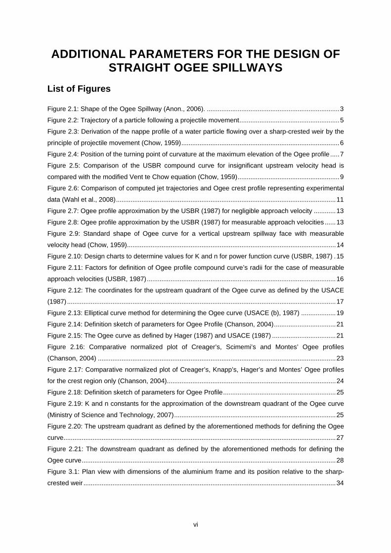
permanganate ....................................................................................................................................... 54 Figure 3.12: Rendered model reflecting the water surface for water flowing over the sharp-crested

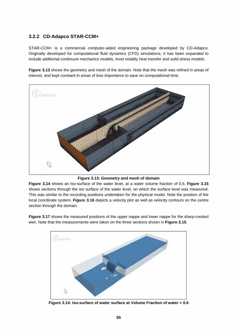
weir at an equivalent discharge of 110 l/s ............................................................................................. 54 Figure 3.13: Geometry and mesh of domain ........................................................................................ 55 Figure 3.14: Iso-surface of water surface at Volume Fraction of water = 0.6 ....................................... 55 Figure 3.15: Sections of Iso-surface of water surface at Volume Fraction of water = 0.6 .................... 56 Figure 3.16: Velocity plots on centre section through domain. ............................................................. 56 Figure 3.17: Nappe measurements ...................................................................................................... 57 Figure 5.1: Spioenkop dam inundation basin and normalized velocity distribution upstream of dam

wall ........................................................................................................................................................ 65 Figure 5.2: Definition sketch of asymmetrical flow ................................................................................ 66 Figure 5.3: Definition sketch of flow orientation relative to dam wall .................................................... 67 Figure 5.4: Flow diagram indicating the use of the VC relationship to describe the Ogee spillway for

asymmetric upstream flow conditions ................................................................................................... 68 Figure 6.1: Approach channel requirements for designing a fully contracted sharp-crested weir (ISO

1438, 2008) ........................................................................................................................................... 70 Figure 6.2: Plate requirements for a sharp-crested weir (ASTM International, 2001; ISO 1438, 2008)

.............................................................................................................................................................. 71 Figure 6.3: Estimation of effective weir widths for ratios of b/B (ISO 1438, 2008) ............................... 72 Figure 6.4: Estimation of discharge coefficient for ratios of h/p (ISO 1438, 2008) ............................... 72

viii


List of Tables Table 2.1: Methods for approximation of the Ogee curve ....................................................................... 4 Table 2.2: Ogee profile approximation by the USBR (1987) for negligible approach velocity .............. 12 Table 2.3: Standard shape of Ogee curve for a vertical upstream spillway face with measurable

velocity head (Chow, 1959) ................................................................................................................... 14 Table 2.4: 2-dimensional flow parameters required to approximate Ogee curve ................................. 26 Table 3.1: Components of the physical model ...................................................................................... 30 Table 3.2: Distances along the crest where the recordings where recorded ........................................ 32 Table 3.3: Measures which were taken to ensure smooth upstream flow conditions .......................... 32 Table 3.4: Definition of Cartesian co-ordinate system .......................................................................... 36 Table 3.5: Installation of water level meters in stilling columns ............................................................ 39 Table 3.6: Summary of the scenarios modelled as well as their associated “Identification Reference”

.............................................................................................................................................................. 41 Table 3.7: Results obtained from the physical modelling ..................................................................... 46 Table 3.8: Thermo-physical properties of the fluid ................................................................................ 50 Table 3.9: Simulation parameters applied for the various analyses performed .................................... 51 Table 3.10: Parameter set for the different numerical models .............................................................. 58 Table 3.11: Different geometric layouts and sections of the iso-surfaces captured from the CFD

modelling ............................................................................................................................................... 58 Table 3.12: Nappe profiles comparison between the CFD analyses and the theoretical approximation

by the USACE (a) .................................................................................................................................. 60 Table 3.13: Design parameters used for the approximation of the theoretical and recommended Ogee

profiles ................................................................................................................................................... 61 Table 4.1: Key aspects to consider when comparing physical modelling with CFD models (Kuzmin,

n.d.) ....................................................................................................................................................... 62 Table 4.2: Comparison of the theoretical and physical model’s recorded Ogee profile with XFlow™ &

STAR-CCM+ CFD modelled Ogee profiles .......................................................................................... 63 Table 6.1: Discharge coefficient for un-contracted (full width) weirs (Bagheri & Heidarpour, 2010; ISO

1438, 2008) ........................................................................................................................................... 73 Table 6.2: Discharge coefficient for contracted weirs ........................................................................... 73 Table 6.3: Observed parameters and calculated discharge coefficients .............................................. 74

1


1 INTRODUCTION

1.1 Background The Ogee spillway relationship (USBR, 1987; Vischer & Hager, 1999) is used to define the required profile of the spillway section of a dam or hydraulic structure. The Ogee relationship describes the bottom nappe associated with a sharp-crested weir. The current relationship accommodates the influence of the unit discharge, the angle of inclination of the upstream wall face, as well as the relationship of upstream pool depth to the total upstream energy at the apex of the structure. In cases where the discharge flow rate exceeds the design flow rate the nappe coheres to surface of the spillway and a sub-atmospheric pressure region is generated that could lead to cavitation (Savage & Johnson, 2001; Momber, 2000). Cavitation usually occurs during a unit discharge, in excess of the design head, when the surface pressure could reduce at positions along the spillway to sub-atmospheric pressure. This may cause the formation of vapour cavities. The vapour cavities (also referred to as miniscule air bubbles) will progress along the flow path due to the high flow velocity on the spillway to a region downstream where sufficient pressure is available leading to the collapse of the air vacuum. This generates localized high pressures. Should these vapour cavities collapse near the spillway structure, there will be some superficial damage to the spillway’s surface where the vapour bubble has collapsed. This cavitation damage can ultimately result in substantial erosion and, if ignored, will subsequently cause failures of the spillway chute. Minute cracks, offsets and increased surface roughness intensify this cavitation process. The extent of cavitation damage is a function of the cavitation indices at key locations on the spillway chute and the duration of flow over the spillway. This emphasizes the need for a geometric, accurate and precise spillway profile to reduce the possibility of sub-atmospheric pressure formation (U.S. Army Corps of Engineers, 2009). The current Ogee spillway relationship lacks to incorporate the asymmetrical cross sectional upstream geometry of the spillway, the relative orientation of the spillway with regard to the approaching flow and the curvature of the spillway in relation to the depth of the structure. The Water Research Commission has funded the research on Ogee spillways which was conducted at the University of Pretoria. The research was aimed to review additional parameters that needs to be considered when designing an Ogee spillway. These parameters will contribute to extend the numerical relationship for Ogee spillways of straight wall structures and to accommodate the effect of an asymmetrical upstream cross sectional as well as the relative orientation of the wall dam wall in relation to the flow direction. The curvature of the dam wall was not reviewed during this research. The focus of this report can be summarised as follows:

1 Provide a theoretical overview of the development from past to present numerical relationships used to define the geometry of an Ogee spillway by considering the most renown relationships;

2 Reflect from experimental quantification, the influence on the geometric form of the Ogee curve caused by the flow in an asymmetrical approach channel, upstream of a straight wall;

2

3 Reflect from experimental quantification, the influence on the geometric form of the Ogee curve caused by the flow in a skew orientated approach channel, upstream of a straight wall;

4 Validate the experimental quantification of the Ogee curve with similar numerical simulations with the aid of computational fluid dynamics (CFD);

5 Reflect the conceptual development of a procedure to incorporate the influence of upstream 3-dimensional flow conditions that can be used for the design of Ogee spillways; and

6 Additional: Determine the variation of the discharge coefficient for different flow approach conditions for a sharp-crested weir compared to ISO 1438 Hydrometry - Open Channel flow measurement using thin plate weirs (ISO 1438, 2008).

The progress of this research has been captured in a number of deliverables (DL1 to DL5) discussed and reviewed by the reference group. These deliverables can be provided on request if required. The above mentioned focus areas of the research were discussed in the following Sections. 1.2 Layout of this report Section 1: Background and focus of research study. Section 2: Provide the theoretical overview of relationships used for approximating the geometry

of Ogee spillways. Section 3: Reflect the construction of a physical model and the setup of the numerical model to

verify the influence on the geometric variation of the Ogee curve caused by the upstream flow condition with a straight wall.

Section 4: Comparing the results from numerical analyses with the observed physical model’s results.

Section 5: Reflect the conceptual development of a procedure to incorporate the influence of the upstream flow conditions on the geometric curve of the Ogee spillway.

Section 6: Develop relationship for the required adaptation of the Ogee spillway section to incorporate the upstream flow conditions for a straight wall.

Section 7: Provide software for the calculation of the geometry of the Ogee spillway. Section 8: The variation of the discharge coefficient for different flow approach conditions for a

sharp-crested weir compared to ISO 1438 Hydrometry.

3

2 LITERATURE REVIEW

2.1 Introduction to Ogee Spillways Chadwick et al. (2004) described a spillway as a structure that is a carefully designed passage used to provide for the controlled release of water from a dam into a downstream area, typically being the river that was being dammed. Spillways release floods safely so that the water does not overtop the structure which could lead to damage or even failure of the dam. The Ogee spillway is commonly used and the typical profile is shown in Figure 2.1. The nappe trajectory on which the Ogee spillway is based, varies with head (Hd), implying that the crest profile is derived on a specific head or discharge (i.e. the design head).

Figure 2.1: Shape of the Ogee Spillway (Anon., 2006).

The geometry of an Ogee spillway profile is based on a physical analysis of the shape produced by a ventilated jet of water flowing over a sharp-crested weir. The shape of the curve was determined by measuring the vertical distance from a datum to the underlying nappe of the jet flowing over the weir along the length of the jet in the direction of flow. Difficulties existed when a single equation was fitted to the upstream quadrant (i.e. the crest) of the spillway. The United States Bureau of Reclamation (USBR, 1987) and US Army Corps of Engineers (USACE, 1970) estimated the profile by means of a series of circular curves. The efficiency of the Ogee spillway is vastly dependent on the curvature of the crest immediately upstream of the highest point on the crest defined as the crest axis. With any sudden change in curvature or slight discontinuity it will cause a disruption of the boundary layer sheet of water and could lead to flow separation and cavitation. According to Murphy (1973), removing any small discontinuities (intersection points of circular curves) between the upstream face and upstream quadrant of the spillway could result in a three percent increase of the coefficient of discharge (USACE, 1992).

Hd

Surface/top nappe

Bottom nappe Upstream quadrant

Downstream quadrant

4

2.2 Categorization of Ogee relationships A wealth of literature is available on the approximation of the Ogee profile for spillway design and several endeavours have been made developing a relationship that would be able to mathematically describe the shape of the Ogee curve considering 2-dimensional flow parameters. Unfortunately in most cases the flow over an Ogee spillway cannot be considered merely as a 2-dimensional flow state. The asymmetricity of valleys and topographical approach channels where spillways are constructed will influence the flow pattern and velocity distribution upstream of the spillway. Neglecting these 3-dimensional flow behaviours may result in an insufficient design of the Ogee spillway structure. The most obvious 3-dimensional flow parameters that influence the geometry of the Ogee profile include (van Vuuren, et al., 2011):

• The relative orientation of the spillway with regard to the approaching flow;

• The asymmetrical cross sectional approach channel upstream from the spillway; and

• The curvature of the spillway (not considered for this study). Some of the well-regarded approximations are described in the following section and were grouped into two categories (Table 2.1):

a. Approximation of the Ogee curve by means of first principles of projectile movement; and b. Approximation of the Ogee curve by means of empirical methods.

Table 2.1: Methods for approximation of the Ogee curve

Approximation of the Ogee curve based on the principles of projectile movement

Approximation of the Ogee curve based on experimental methods

Description Description

Ven te Chow (1st Principles) (Chow, 1959) United States Bureau of Reclamation (USBR,

1987)

Ven te Chow (Modified) (Chow, 1959) United States Army Corps of Engineers (USACE,

1970)

Brink Velocity (Wahl, et al., 2008) United States Army Corps of Engineers (USACE

(b), 1987) Hager (1987) Creager (Chanson, 2004) Scimeni (Chanson, 2004) Montes (Chanson, 2004) Knapp (Chanson, 2004)

CE-05016 (Ministry of Science and Technology,

2007)

2.3 Approximation of the Ogee curve by means projectile movement

2.3.1 Preamble Projectile movement of any particle is defined as a form of motion where a particle is moving obliquely near the earth’s surface due to an initial force exerted onto it. The particle will move along a curved path under the action of gravity. From the equation of motion (Equation 2.1) it is possible to determine the two-dimensional displacement of a particle assuming constant acceleration acts onto it and neglecting all external forces (drag force etc.):

5

s=vot+1

2at2

Equation 2.1 Where s - displacement of the particle for a time duration of t seconds (m) vo - the initial velocity of the particle (m/s) a - constant acceleration acting onto the particle (m/s2) t - time duration of acceleration acting onto the particle (sec.) Assuming that gravitational acceleration is constant and act only in the vertical direction, it is possible to determine the trajectory of a projectile by breaking it up into two components: a. horizontal displacement (x) and b. vertical displacement (y) as illustrated in Figure 2.2. Making use of Equation 2.1 the horizontal and vertical components of the trajectory can be estimated in 2-dimensions by combining Equation 2.2 and Equation 2.3.

Figure 2.2: Trajectory of a particle following a projectile movement

x=vot cosθ Equation 2.2

y=vot sinθ+1

2at2

Equation 2.3 Where: θ - projectile launch angle (degrees) The trajectory of the projectile can be determined by eliminating the time component (t) from Equation 2.2 and Equation 2.3 to obtain Equation 2.4.

y= tan θ ·x+a

2vo cos2 θ·x

Equation 2.4

6

2.3.2 Ogee curve approximated by Ven te Chow from 1st Principles of projectile movement

Vent te Chow (1959) indicated that the geometric shape of a water particle flowing over a sharp-crested weir can be interpreted by the principle of projectile movement (Figure 2.3). Similar to the assumption of projectile movement in Section 2.3.1 it was assumed that the horizontal velocity component of the flow particle is not experiencing any gravitational forces implying a constant horizontal movement. The only force acting onto the water particle would be in the vertical direction that is caused by gravity.

Figure 2.3: Derivation of the nappe profile of a water particle flowing over a sharp-crested weir

by the principle of projectile movement (Chow, 1959) For a predefined time duration the water particle at the lower nappe will experience a movement in the horizontal (x) and vertical (y) plane as expressed by Equation 2.5 and Equation 2.6.

x=vot cosθ Equation 2.5

y=-vot sinθ+1

2gt2+C'

Equation 2.6 Where: x - horizontal displacement during a time duration t (m)

y - vertical displacement during a time duration t (m) vo - the initial velocity of the water particle (m/s) g - gravitational acceleration acting onto the water particle (m/s2) t - time duration for assessment of particle (sec.) θ - angle of inclination (degrees) C’ - the vertical displacement of the particle at x = 0 m (m) Research indicated that the vertical displacement of the particle at x = 0 m (C’) is equal to the vertical distance between the highest point of the nappe and the elevation of the crest (Chow, 1959). Rajaratnam et al. (1968) indicated that the vertical position C’ can be empirically estimated Equation

7

2.7 and the horizontal distance (f’) to this co-ordinate measured from the crest can be estimated by Equation 2.8. These experiments by Rajaratnam et al. were done for a confined weir (un-contracted). This position is known as the turning point of curvature (Tp) and is depicted in Figure 2.4.

Figure 2.4: Position of the turning point of curvature at the maximum elevation of the Ogee

profile

C'=0.112·Hd-0.4vo

2

2g

Equation 2.7

f'=0.250·Hd-0.4vo

2

2g

Equation 2.8 Where: Hd - measured water depth on the crest (m) The lower surface of the nappe can be determined by eliminating the time component (t) from Equation 2.5 and Equation 2.6. A normalized form of the equation can be obtained by dividing each term by the total energy head upstream of the crest (Equation 2.9).

Y

He=A

x

He

2

+Bx

He+C

Equation 2.9 Where:

A - gHe

2v02 cos2 θ

B - - tan θ

C - C'

He

He - total energy head upstream of crest (m)

8

2.3.3 Ogee curve approximated by Ven te Chow (Modified) From the normalized form of the projectile trajectory of the nappe over an aerated vertical sharp-crested (Equation 2.9) as derived by Vent te Chow (1959), a general parabolic equation for the Ogee curve was proposed by Chow, Equation 2.10. By adding the term D to the equation, the upper surface of the Ogee nappe can also be determined. Chow has derived the parabolic equation to determine the Ogee nappe curve for ratios of x/He > 0.5 and Ha/He > 0.2 based on the experimental data taken from the USBR, Hinds, Creager and Justin, Ippen and Blaisdell. The values for the constants for A, B, C and D can be determined from Equation 2.11 to Equation 2.14. Chow indicated that for ratios of x/He < 0.5 the hydrostatic pressure within the nappe in the vicinity of the weir crest is above atmospheric pressure because of the convergence of the stream lines. Consequently, forces other than gravity are acting onto the nappe, which makes the principle of projectile movement fallacious.

Y

He=A

x

He

2

+Bx

He+C+D

Equation 2.10 With:

A=-0.425+0.25Ha

He

Equation 2.11

B=0.411-1.603Ha

He- 1.568

Ha

He

2

-0.892Ha

He+0.127

Equation 2.12

C=0.150-0.45Ha

He

Equation 2.13

D=0.57-0.02 10m 0.2e10m Equation 2.14

Where:

m=Ha

He-0.208

Ha - velocity head V2

2g (m)

He - total energy head upstream of crest A comparison of the USBR (Figure 2.7) compound curve for insignificant upstream velocity head is compared with the modified Vent te Chow relationship (Equation 2.10) in Figure 2.5. The modified Vent te Chow relationship (Equation 2.10) seems to underestimate the gravitation acceleration exerted onto the particle resulting in the trajectory of the nappe of water particle to be more conservative.

9

Figure 2.5: Comparison of the USBR compound curve for insignificant upstream velocity head

is compared with the modified Vent te Chow equation (Chow, 1959) 2.3.4 Ogee curve approximated by Wahl et al. (2008) Wahl et al. (2008) indicated that the prediction of the trajectory of a free falling jet of water described by Vent te Chow (1959) may be flawed, producing a water jet trajectory that is much too flat. This may be a valid argument by Wahl et al., as one of the principal assumption made during the derivation of Equation 2.9 was that no external force is acting onto the water particle. Through algebraic manipulation, the trajectory equation can be restated in terms of the velocity head (Equation 2.15). Wahl et al. stipulate that using Equation 2.9 as it is may overestimate the jet trajectory by as much as 70% if the flow is exactly critical at the crest overtopping position. In an ideal environment, this would have not been a problem; however, external forces like the drag force (air’s resistance to movement) will be acting onto the lower nappe of water, and should thus be considered.

y=x tanθo-x2

4Ha cos2 θo

Equation 2.15 Where: x - horizontal displacement (m)

y - vertical displacement (m) Ha - the velocity head (m) θo - angle of inclination (degrees)

-0.1

0.0

0.1

0.2

0.3

-0.1 0.0 0.1 0.2 0.3V

ertic

al y

-sca

leHorizontal x-scale

Ven te Chow 1st Principles Mod

USBR Compound

Modified Ven te Chow equation only valid for

x/He > 0.5 and Ha/He > 0.2

10

The USBR (1987) has also noticed a discrepancy with Equation 2.9 and considered including the depth of flow and a coefficient, K in the denominator (Equation 2.16). The notion of including the coefficient was to account for the external forces acting onto the water nappe, such as jet breakup and wind resistance.

y=x tan θo-x2

4K d+Ha cos2 θo

Equation 2.16 Where: d - the depth of flow over the crest (m) K - constant less or equal to 1 When comparing Equation 2.16 and Equation 2.15, which was both derived from the projectile motion equation, it is clear that they are not equivalent, even when K = 1. According to Wahl et al. (2008) Equation 2.16 would only be accurate if the total overtopping head could be converted to velocity head. However, in most cases this is not possible since a nearly hydrostatic pressure profile exists in the flow until the flow passes over the crest and part of the energy is in the form of pressure head. Instead of including all the external forces acting onto the jet of water mathematically, Wahl et al. (2008) considered an empirical relationship known as the “brink velocity” that reflects the velocity when the water flows over the edge of the crest. The brink velocity was derived experimentally by (Rouse, 1936) and is approximated by Equation 2.17.

vb=0.808 2gHd

Equation 2.17 Where: vb - brink velocity (m/s)

Hd - water depth on the crest (m) Wahl et al. (2008) recommends that Equation 2.15 should be used in conjunction with the brink velocity head as reflected by Equation 2.17. It is also further suggested that a 7° downward deflection (θ) of the flow streamlines should be considered for the mid-section of the trajectory (Henderson, 1966). The trajectory estimated by Wahl et al. (2008) closely matches the profile of the Ogee geometry estimated by the compound curves as determined by USBR (1987). A comparison of these curves is depicted in Figure 2.6.

11

Figure 2.6: Comparison of computed jet trajectories and Ogee crest profile representing

experimental data (Wahl, et al., 2008)

2.4 Approximation of the Ogee curve by means of experimental methods

2.4.1 Preamble Profiles of Ogee’s have been experimentally developed for a range of dam heights and operating heads (He/P ratios). This information has mainly been published by the US Bureau of Reclamation and the US Army Waterways Experimental Station (Chadwick, et al., 2004). The relationship of the Ogee curve approximated by different experimental setups and researchers are described in the following paragraphs.

2.4.2 Ogee curve approximated by the USBR (1987) Research conducted by the United States Bureau of Reclamation (USBR, 1987) has resulted in the approximation of the Ogee profile by means of a series of compound circular curves. The conclusion of this research resulted in the formation of a relationship that numerically describes the shape of the Ogee curve with relation to the design head of the system. According to the USBR (1987), the shape of the Ogee profile is dependent on the following factors:

• Design head;

• Upstream wall face inclination; and

• Pool depth, which in turn influences the approach velocity. All these factors are 2-dimensional flow parameters consequently requiring the extension of the relationship to include 3-dimensional flow parameters. The relationship for the curve derived by the USBR consists of two quadrants: the first being that portion upstream of the apex of the Ogee profile, and the second being that downstream of the apex of the Ogee profile. The upstream quadrant can be defined in two manners, namely as a single curve in combination with a tangent (section 2.4.4), or as a compound circular curve; and is most often defined using the latter. The downstream portion can also be described in two manners, namely as a power function or a compound circular curve. The approximate Ogee profile for a crest with a vertical upstream face and negligible approach velocity can be estimated by the compound circular curve configuration that comprises for the upstream quadrant of the spillway of two arcs of differing radii and points of origin, as shown in Figure 2.7. The downstream quadrant of the profile is estimated by five circular curves of differing radii and points of origin. Vischer & Hager (1999) indicated that the ratio of velocity head to design head is

12

negligible, provided the head over the weir is greater than 100 mm and smaller than half of the pool depth. Table 2.2 depicts the Ogee profile’s numeric approximation by the USBR (1987) for negligible approach velocity numerically.

Table 2.2: Ogee profile approximation by the USBR (1987) for negligible approach velocity

Radius Radius

magnitude (x·Ho) (m)

x-coordinate origin (x·Ho)

(m)

y-coordinate origin (y·Ho)

(m)

x-coordinate start (x·Ho)

(m)

x-coordinate end (x·Ho)

(m)

y-coordinate start (y·Ho)

(m)

y-coordinate end (y·Ho)

(m)

R1 0.235 -0.082 0.247 -0.284 -0.147 0.127 0.021

R2 0.530 0.000 0.530 -0.147 0.000 0.021 0.000

R3 0.825 0.000 0.825 0.000 0.217 0.000 0.029

R4 1.410 -0.153 1.389 0.217 0.583 0.029 0.187

R5 2.800 -0.880 2.575 0.583 1.230 0.187 0.734

R6 6.500 -3.668 5.007 1.230 1.840 0.734 1.556

R7 12.000 -8.329 7.927 1.840 2.758 1.556 3.336

Note: Ho - water depth measured upstream of the crest (m) He - total energy head upstream of crest, depicted as Ho in Figure 2.7 (m) Hd = He - approach velocity negligible (m)

The USBR (1987) approximate the Ogee curve in cases where the approach velocity cannot be neglected by means of a compound circular curve configuration that comprises of two arcs of differing radii and points of origin, as shown in Figure 2.8 for the upstream quadrant of the spillway and a power function curve for the downstream quadrant of the spillway. For the most general form of Ogee profiles, like in the case of a vertical upstream spillway face, the USACE has developed on the basis of the USBR several standard shapes (Chow, 1959). An example of such a standard shape is depicted in Figure 2.9 and numerically reflected in

13

Table 2.3. Determining the radii of the compound curves for any other configuration, Figure 2.10 can be used that relate the ratio of approach velocity and the measured crest water depth to the specific radii of the compound circular curves to yield the Ogee profile USBR (1987).

Figure 2.7: Ogee profile approximation by the USBR (1987) for negligible approach velocity

Figure 2.8: Ogee profile approximation by the USBR (1987) for measurable approach velocities

14

Table 2.3: Standard shape of Ogee curve for a vertical upstream spillway face with measurable velocity head (Chow, 1959)

Radius Radius magnitude

(x·Hd) (m)

x-coordinate start (x·Hd) (m)

x-coordinate end (x·Hd) (m)

R1 0.200 -0.282 -0.175

R2 0.500 -0.175 0.000

The power function describing the downstream quadrant of the Ogee curve is given by Equation 2.18 and includes variables K and n that is a function of the upstream face geometry of the spillway (USBR, 1987). The values of K and n can be graphically derived from Figure 2.10. The power function describing the downstream quadrant of the Ogee curve the same as that of the USACE and IS: 6934-1998 downstream quadrant, as explained in greater detail in the section 0 and section 2.4.4 respectively.

y

He=-K·

x

He

n

Equation 2.18 Where:

y - Vertical distance from the apex to the curve (m) He - total energy head upstream of crest, depicted as Ho in Figure 2.10 (m) K - Constant, dependent on the upstream inclination and approach velocity x - Horizontal distance from the apex to the curve (m) n - Constant, dependent on the upstream inclination and approach velocity

Figure 2.9: Standard shape of Ogee curve for a vertical upstream spillway face with measurable velocity head (Chow, 1959)

15

Figure 2.10: Design charts to determine values for K and n for power function curve (USBR,

1987)

16

Figure 2.11: Factors for definition of Ogee profile compound curve’s radii for the case of

measurable approach velocities (USBR, 1987)

17

2.4.3 Ogee curve approximated by the UASCE (1970) The U.S. Army Corps of Engineers (USACE, 1970, revised 1987) suggested a revised compound circular curve to describe the upstream quadrant of the Ogee curve. The upstream quadrant originally defined in Figure 2.8 and Figure 2.9 by the USBR (1987), resulted in a surface discontinuity at the vertical spillway face. Model studies at the U.S. Army Waterways Experiment Station indicated that the incorporation of a small arc with radius = 0.04Hd improved pressure conditions, reduced possible cavitation of the spillway crest and increased the discharge coefficients for heads exceeding the design head (USACE (a), 1987). The coordinates for the origins of curvature and transition points of the improved design is schematically indicated in Figure 2.12 together with a table that reflect the numerical values of the origins. Recent model studies have verified the use of an elliptical upstream quadrant design that was also discussed by the USACE (1992) and reflected in section 2.4.4 of this report. The USACE suggest that the method, depicted by the elliptical curve should be used for future spillway design and that the Standard Shape Criteria as presented in this section, must only be retained for reference purposes.

Figure 2.12: The coordinates for the upstream quadrant of the Ogee curve as defined by the

USACE (1987)

18

The downstream quadrant of the Ogee curve is defined by a power function (Equation 2.19) similarly to the description used by the USBR (1987). The USACE (1987) define the K and n coefficients in the equation as 0.5 and 1.85, respectively. Therefore is the downstream quadrant of the USACE Ogee curve in Figure 2.12 the same as the downstream quadrant defined by the USBR in Figure 2.8.

y

Hd=-K·

x

Hd

n


Hd - water depth measured upstream of the crest (m)

2.4.4 Ogee curve approximated by USACE (b) (1987) The Bureau of Indian Standards (IS: 6934-1998) has adapted this design procedure for Ogee spillways in the national standards (Anon., 2006). The USACE (1987) found that their earlier attempts to fit circular arcs to the profile of the lower nappe of the flow over a sharp-crested weir produced surface discontinuities at the weir’s crest. Even with adding the short-radius arc tangent to the vertical face, the intermediate-radius arc discontinuities still existed at the weir’s crest although this ascertained to be an improvement of the original design. The U. S. Army Engineer Waterways Experiment Station (WES) conducted physical model studies to compare the hydraulic performance of the most commonly used upstream quadrant design procedures and concluded that the short-radius arc method (Section 2.4.4) and an elliptical curve method appeared to yield the most acceptable results, although both methods were only considering 2-dimensional flow parameters (USACE (b), 1987). For the upstream quadrant Murphy (1973) found that, by systematically varying the axes of an ellipse with depth of approach, it was possible to approximate the lower nappe surfaces similar to that estimated by the USBR (1987). Murphy also indicated that any sloping upstream of the spillway face could be used with little loss of accuracy if the slope became tangent to the ellipse calculated for a vertical upstream face. In 1973 WES published results of preliminary studies done to verify a design procedure incorporating an elliptical upstream quadrant developed from the USBR data (USACE (b), 1987). The procedure was verified for high spillways during these tests and a comprehensive test program with a wide range of approach velocities, upstream face slopes, and head ratios was conducted at WES from 1977 to 1982. Murphy (1973) indicated that the quadrant of an ellipse in which the axes systematically varied with depth of the approach channel would fit the measured data, except that the ellipse quadrants would extend upstream of the position of the sharp-crested weir used to generate the nappe form to become tangent to the vertical of the spillway wall. This extension is more pronounced when P/Hd is relatively small. Translating the origin of the elliptical curve of the upstream quadrant to the crest of the Ogee profile and referencing the positive y-direction downwards (Figure 2.13), the elliptical curve can be mathematically expressed by Equation 2.20 (USACE (b), 1987).

19

Y=B 1- 1-X2

A2


A - coefficient to be solved from normalizing by the design head Hd Figure 2.13 B - coefficient to be solved from normalizing by the design head Hd Figure 2.13

X - horizontal co-ordinate of Ogee profile Y - vertical co-ordinate of Ogee profile

In the case of the downstream quadrant of the Ogee curve the general power function as proposed by the USBR (1987) is still valid (Equation 2.18). For high spillways where the ratio of velocity head (Ha) to the design head (Hd) is less than 0.06, K and n coefficients of 0.5 and 1.85 are recommended. As the depth of the approach channel decreases, the approach velocities increase proportionally and the Ogee profile will in essence become flatter to match the partially suppressed vertical contraction of the nappe. Experimental data by WES for sharp-crested weirs found that the downstream quadrant of the spillway can be estimated by maintaining the form of Equation 2.18 with n = 1.85 and varying K with approach depth. The K value can be determined from Figure 2.13.

Figure 2.13: Elliptical curve method for determining the Ogee curve (USACE (b), 1987)

20

2.4.5 Ogee curve approximated by Hager (1987) Vischer & Hager (1999) noted that the Ogee curve approximated by the USBR (1987) and USACE (1987) was made up of multiple compound circular curves. This was disadvantageous as there were sudden discontinuities on the Ogee profile that occurred at each of the transition points where the arcs intersected. The concern with this was explained by pointing out the shortcomings of the geometry with regards to:

• Computational solutions of the approach geometry was not possible due to the discontinuity of curvature at the transition points between arcs; and

• Cavitation problems arising at the discontinuities of the arcs during high flow. Hager (1987) approximated the Ogee curve by an alternative smooth curve determined by reordering the co-ordinates given by the USACE (1987) onto a transposed co-ordinate system. Hager has transferred the origin of the co-ordinate system used by the USACE located at the highest point of the Ogee’s crest to the minimum horizontal distance value. The Ogee curve suggested by Hager can be mathematically calculated by means of Equation 2.21.

Z*=-X*lnX*, for X*>-0.2818 Equation 2.21

Where: X* and Z* are transformed coordinates based on the three arc compound circular curve of USACE (1987)

and

X*=1.3055· X+0.2818

Z*=2.7050· Z+0.1360 With

X=x

Hd

Z=z

Hd

Where: Hd - water depth measured upstream of the crest (m) x - horizontal co-ordinate of Ogee profile y - vertical co-ordinate of Ogee profile

In 1991, Hager has simplified the transformed coordinates of X* and Z* to obtain an equation for the same Ogee curve in Cartesian format equations by making use of Equation 2.22

Y

Hdes-∆z=0.136+0.482625

X

Hdes-∆z+0.2818 · ln 1.3055

X

Hdes·∆z+0.2818

Equation 2.22 Valid for:

-0.498<X

Hdes-∆z<0.484

Where: Hdes and ∆z are defined in Figure 2.14

21

Figure 2.14: Definition sketch of parameters for Ogee Profile (Chanson, 2004)

A comparison of the USACE (1987) and Hager (1987) Ogee curves are depicted below in Figure 2.15. For design purposes the difference between the two profiles are usually negligible and differences only exits on the downstream quadrant of the Ogee curve.

Figure 2.15: The Ogee curve as defined by Hager (1987) and USACE (1987)

In the following sections a summary (section 2.4.6 to section 2.4.9) of some of the longstanding Ogee curve relationships are given by Hubert Chanson (2004). These relationships can be in many ways

-0.1

0.0

0.1

0.2

0.3

0.0 0.1 0.2 0.3

Ver

tical

y-s

cale

Horizontal x-scale

USACE (1987) Hager (1987)

22

be regarded as the origin of the mathematical relationship of the Ogee curve and date as far back as 1888 from which Creager in 1917 has used the original data of Bazin in 1886-1888 to develop one of the first mathematical extension of the Ogee curve. The most common, early century Ogee profiles used, were the U. S. Army Engineer Waterways Experiment Station (WES) by Scimemi in 1930 and the Creager profile (Chanson, 2004). These relationships only considered the 2-dimensional flow parameters.

2.4.6 Ogee curve approximated by Creager, 1917 (Chanson, 2004)

Y=0.47·X1.8

Hdes-∆z 0.8 valid for X ≥ 0;


2.4.7 Ogee curve approximated by Scimeni, 1930 (Chanson, 2004) The WES standard Ogee curve is based upon detailed observations of the lower nappe of sharp-crested weir flows.

Y=0.50·X1.85

Hdes-∆z 0.85 valid for X ≥ 0;


2.4.8 Ogee curve approximated by Montes, 1992 (Chanson, 2004) In 1992, Montes developed a continuous spillway profile with continuous curvature radius on curvilinear co-ordinate system that acts along the crest shape. The lower asymptote of the relationship: i.e. for small values of s/(Hdes - ∆z) was approximated by Equation 2.23; with a smooth variation between the asymptotes by Equation 2.24 and the upper asymptote: i.e. for large values of s/(Hdes - ∆z) estimated by Equation 2.25.

R1

Hdes-∆z=0.05+1.47·

s

Hdes-∆z

Equation 2.23

R

Hdes-∆z=

R1

Hdes-∆z1+

Ru

R1

2.6251

2.625

Equation 2.24

Ru

Hdes-∆z=1.68·

s

Hdes-∆z

1.625


Hdes and ∆z are defined in Figure 2.14 s - curvilinear co-ordinate along the crest shape R - radius of curvature of the crest (m)

23

A comparative plot of Creager’s, Scimemi’s and Montes’ Ogee profiles are reflected in Figure 2.16. Similar results is obtained by Scimemi’s and Montes’ with Creager estimating a greater Ogee profile for similar conditions. The axis’s of the plot was normalized by dividing the X and Y co-ordinates by (Hdes - ∆z) respectively (Chanson, 2004).

Figure 2.16: Comparative normalized plot of Creager’s, Scimemi’s and Montes’ Ogee profiles

(Chanson, 2004)

2.4.9 Ogee curve approximated by Knapp, 1960 (Chanson, 2004) In 1960, Knapp approximated the crest of the Ogee profile by Equation 2.26. A comparative plot of Creager’s, Knapp’s, Hager’s and Montes’ Ogee profiles for the crest region only are reflected in Figure 2.17.

Y

Hdes-∆z=

X

Hdes-∆z- ln 1+

X

0.689 Hdes-∆z


Hdes and ∆z are defined in Figure 2.14

24

Figure 2.17: Comparative normalized plot of Creager’s, Knapp’s, Hager’s and Montes’ Ogee

profiles for the crest region only (Chanson, 2004)

2.4.10 Ogee curve approximated by CE-05016 (Ministry of Science and Technology, 2007)

In the document published by the Ministry of Science and Technology (2007): CE-05016, the upstream quadrant of the Ogee profile is approximated by Equation 2.27. CE-05016 stipulates that the vertical face of the spillway should be tangential to the approximated Ogee curve and should have a zero slope at the crest axis to ensure that there is no discontinuity along the upstream and downstream quadrants of the Ogee curve.

Y=0.724 X+0.270Hd

1.85

Hd0.85 +0.126Hd-0.4315Hd

0.375· X-0.270Hd0.625


Hd - water depth measured upstream of the crest (m) X - horizontal co-ordinate of Ogee profile Y - vertical co-ordinate of Ogee profile

The maximum absolute value of X is 0.270Hd, corresponding to a y-value equal to 0.126Hd when the upstream face of the spillway is vertical as depicted in Figure 2.18.

25

Figure 2.18: Definition sketch of parameters for Ogee Profile

(Ministry of Science and Technology, 2007) The downstream quadrant of the Ogee curve is represented by the same general power curve function as described by the USBR (1987) (Equation 2.19). However, the K- and n-values are constants, which depend upon the inclination of the upstream face of the spillway and can be obtained for a variety of upstream face spillway configurations, with the tangent β as the angle which the upstream face makes with the vertical.

y

Hd=-K·

x

Hd

n


Hd - water depth measured upstream of the crest (m)

Figure 2.19: K and n constants for the approximation of the downstream quadrant of the Ogee

curve (Ministry of Science and Technology, 2007)

26

2.5 Summary and comparison of Ogee profile formulae In this section the different Ogee relationships for the prediction of the bottom nappe across a sharp crested weir is firstly discussed for the upstream section followed by a comparison or the relationships for the prediction of the downstream profile (Figure 2.1). Different nuances for the definition of the upstream profile defining the Ogee curve exists as is shown in Figure 2.20. Figure 2.20 displays the approximations of the upstream quadrant of the Ogee curves on one axis based on the assessment of the value for the different parameters reflected in Table 2.4. From the plot of the Ogee curves the USBR (2 circular compound curve), USBR (insignificant approach velocity), USACE (3 circular compound curve), Hager, and CE-05016 plot on more or less the same position with negligible differences.

Table 2.4: 2-dimensional flow parameters required to approximate Ogee curve

2-Dimensional flow parameter

Value Unit

Total head (He) 2.0 m

Angle of inclination (θ) 7.0 degrees

Gravitational acceleration (g) 9.81 m/s2

Average approach velocity (vo) 3.617 m/s

Velocity Head (hv) 0.667 m

Flow depth over weir (Hd) 1.33 m

Upstream depth (Hdes) 7.0 m

Spillway height (P) 5.0 m

(∆z - P)/H 0.20 m

Height to crest (∆z ) 5.20 m

Unit flow rate (q) 4.82 m3/s/m

Note: Notation as described in Figure 2.14

27

Figure 2.20: The upstream quadrant as defined by the aforementioned methods for defining

the Ogee curve The comparison of the calculated downstream quadrants of the Ogee curve are reflected in Figure 2.21. All the approximations of the downstream quadrant of the Ogee curve are within reasonable range of each other only up to a distance of about 2 m downstream from the crest. The Hager relationship is apparently overestimating the downstream quadrant, while the Vent te Chow derivation from 1st Principles underestimates the Ogee downstream quadrant.

-0.1

0.0

0.1

0.2

0.3

0.4

0.5

-0.1 0.0 0.1 0.2 0.3 0.4 0.5V

ertic

al y

-sca

le (m

)Horizontal x-scale (m)

Vent te Chow 1st Principles (1959) USBR (1987)

Wahl (Brink Velocity) (2008) Creager (1917)

Scimeni / WES (1930) Knapp (Crest Profile only) (1960)

USACE Compound Curve (1987) Hager (1987)

USBR (Insignificant approach velocity, 1987) CE-05016

USACE Elliptical Curve (1987)

28

Figure 2.21: The downstream quadrant as defined by the aforementioned methods for defining

the Ogee curve None of the approximations for the calculation of the Ogee curve includes the upstream asymmetricity, orientation of flow relative to the spillway structure or the curvature of the dam wall. The following section of the report consists of an overview of the physical modelling and numerical modelling of the Ogee profile for asymmetrical and skew approach channels.

-2

0

2

4

6

8

10

12

14

16

18

20

22

24

26

28

30

32

-2 0 2 4 6 8 10 12 14 16 18 20 22 24 26 28 30 32V

ertic

al y

-sca

le (m

)Horizontal x-scale (m)

Vent te Chow 1st Principles (1959)

Ven te Chow 1st Principles Modified (1959)

USBR (1987)

Wahl (Brink Velocity) (2008)

Creager (1917)

Scimeni / WES (1930)

USACE Compound Curve (1987)

Hager (1987)

USBR (Insignificant approach velocity, 1987)

CE-05016

USACE Elliptical Curve (1987)

29

3 PHYSICAL AND NUMERICAL MODELLING OF THE OGEE CURVE

3.1 The physical model A physical model of a sharp crested weir was constructed with the objective to determine the influence of the approach channel geometry on the geometric curve of the bottom nappe (Ogee curve). The construction of the physical model was done at the Laboratories of the Department of Water and Sanitation in Pretoria West. In the following paragraphs an overview of the model construction and method applied for the measurement of the Ogee curve is provided. A more detailed description of the model construction, its dimensions and the different scenarios which were reviewed are described in Deliverable 2 (Section 1.1) The description of the physical model study is reflected under the following headings:

• Physical model construction;

• Preparations made to measure the nappe;

• Installation of the variable side walls used to alter the symmetricity of the approach channel;

• Installation of the stage depth meters with OTT-point gauges to determine the upstream flow depth;

• Notation used for describing different flow scenarios;

• Recording positions of Ogee profiles; and

• Physical model results.

3.1.1 Physical model construction The outer boundary of the physical model was constructed by means of plastered brickwork to a height of 1135 mm. The width of the layout was 3106 mm and total length was ± 15 m. In order to prevent failure of the sides due to the hydrostatic pressure exerted onto the structure during filling of the channel upstream of the weir, the boundary walls were reinforced with brickwork columns spaced ± 1500 mm C-C. Water was fed from the constant head tank to the model by means of a perforated tapered steel pipe. This configuration was used to enhance an even distribution of uniform flow upstream of the sharp-crested weir. Table 3.1 reflects some of the components of the model setup.

30

Table 3.1: Components of the physical model

a. Inlet from constant head tank to model b. Upstream view of approach channel

(without the weir)

c. Upstream view of the installation of the sharp-crested weir with side wall installed

d. Downstream view of the installation of the sharp-crested weir without the measuring rig

31

Table 3.1: Components of the physical model continue

e. Bosch Laser Level setup to determine the locations of measuring positions

f. Masking tape used for the preparation to paint the measurement locations of the profiles

g. Seven locations where the Ogee profiles were measured perpendicular to the sharp-crested weir

The Ogee profile was measured downstream from the crest of the sharp-crested weir at 5 or 7 sections respectively for the baseline (symmetric approach conditions) setup and the other scenarios. The sections were measurements of the Ogee profile were recorded are reflected in Table 3.2 and shown in Table 3.1(g). The relative positions of the recording positions are relative to the lefts edge of the spillway, looking upstream.

32

Table 3.2: Distances along the crest where the recordings where recorded

Line colour which identify the position of the cross section

Distance along the crest measured from the left side of the sharp-crested weir

Yellow 1 100 mm

Purple 1 200 mm

White 400 mm

Red 600 mm

Blue 800 mm

Purple 2 1000 mm

Yellow 2 1100 mm

Two specific aspects were of a concern during the recording of the lower nappe:

• Ensuring a uniform upstream flow distribution; and

• Accurate measurement of the bottom nappe. These items were discussed in the subsequent sections of the report.

3.1.2 Ensuring a uniform upstream flow distribution Some of the measures which were taken to ensure a uniform upstream flow distribution are reflected graphically in Table 3.3. These measures included the installation of a perforated steel inlet pipe and the placement of staggered flow straighteners in a honeycomb configuration.

Table 3.3: Measures which were taken to ensure smooth upstream flow conditions

a. 2 halves of a steel drum and rubber flaps were attached to the perforated steel discharge pipe.

b. Flow straighteners staggered in a honeycomb configuration.

33

Table 3.3: Measures which were taken to ensure smooth upstream flow conditions continue

c. View of 50 % HDPE shade net (final installation position was 1 m upstream of the flow straighteners)

3.1.3 Accurate measurement of the bottom nappe In order to measure the Ogee nappe accurately it was required to construct a rigid framework onto which a measuring apparatus could be mounted. The measurement of the Ogee curve had to be precise and measured for each scenario to a common fixed datum. The measuring apparatus had to be installed without interfering with the natural flow of the water over the sharp-crested weir. An aluminium frame made from extruded FlexiLine aluminium profiles, manufactured by PRO-VEY (Pty) Ltd was used for the framework constructed downstream of the sharp-crested weir. The aluminium frame consisted of four column sections fixed to the concrete ground with M12 Fischer bolts to ensure that the structure was firmly held in place, rigid and that no movement was possible during the experimental runs. The positions of the four columns were accurately set out by making use of a Bosch Laser spirit level, chalk lines and semi-circles to determine the mid-line of the structure. The columns were braced at the bottom and top with rectangles that were held in position with three 63 mm x 63 mm aluminium angle support brackets at each corner. This ensured that the structure was rigid and firmly intact. Dimensions of the structure and its position relative to the sharp-crested weir are given in Figure 3.1.

34

Figure 3.1: Plan view with dimensions of the aluminium frame and its position relative to the

sharp-crested weir The “Ogee Point Measurement Instrument” (OPMI) was built using an Insize Vernier height gauge (IVHG) (Figure 3.2). The height gauge comprised of an adjustable main scale, fitted onto a sturdy cast iron footing. The main scale was fitted with a movable mechanism for the measurement of elements with different heights and had a fine adjustment screw for precision measurement. The Vernier scale had a gradation of 0.02 mm. This small piece of aluminium block was fitted to the top of the height gauge. This allowed for the fitment of a HBM linear variable differential transducer (LVDT) to enable the recording of measurements automatically.

Figure 3.2: Insize Vernier height gauge (IVHG) with fine adjustment (accuracy ±0.05 mm, model

no. 1250-450)

35

At the top of the IVHG was a stainless steel tip, isolated with a rectangular piece of Plexiglas. A circuit allowing current to flow from the water to the tip of the height gauge will close the instance the tip of the height gauge touches the water, similar to a water level sensor. A 12 volt light emitting diode (LED) connected to a relay switch will illuminate, indicating that the tip of the height gauge has made contact with the water surface. This enables one to make very precise measurements repetitively without penetrating the bottom profile (Ogee). The circuit used for the OPMI water sensor, is discussed below. The OPMI was fitted with a KEMO® M158 Waterswitch that functioned in the same manner as a water level sensor. The KEMO® M158 Waterswitch and geometric dimensions are reflected in Figure 3.3. Providing a direct current of 500 mA via the 12V power supply, the instance the copper tip of the OPMI touch the lower nappe of the water flowing over the sharp-crested weir, the resistance in the circuit of the Waterswitch is more than the resistance for the current to flow via the water, at this instance the relay switch is triggered and the LED lit up. A schematic layout of the circuit for the Waterswitch was given below in Figure 3.4.

Figure 3.3: KEMO® M158 Waterswitch with geometric dimensions (KEMO®, 2012 (a))

Figure 3.4: Water level sensor circuit (KEMO®, 2011)

36

A right-handed Cartesian axis co-ordinate system was used with the physical model to enable one to define each measuring position on the lower nappe to a unique XYZ-coordinate. All the measurements where made relative to the crest of the weir, thus requiring for each setup to calibrate and record zero position measurements. Measurements were taken at 10 mm intervals in the X-axis direction and at the 7 pre-determined positions along the crest of the sharp-crested weir (Table 3.2). Table 3.4 provides a pictorial sequel of the definition of Cartesian co-ordinate system.

Table 3.4: Definition of Cartesian co-ordinate system

a. Mastercraft 1000 mm rulers fixed to extruded aluminium profiles. Intersection of X and Y axes.

b. OPMI slide mechanism fixed to the Y-axis.

c. XYZ-axis as defined for the physical model.

37

Table 3.4: Definition of Cartesian co-ordinate system continue…

d. Calibration of OPMI taking zero measurements with vertical copper point at each measuring position along the crest of the weir.

e. Calibration of OPMI taking zero measurements with rotated copper point at each measuring position along the crest of the weir.

f. Taking measurements of lower nappe

with vertical copper point. g. Taking measurements of lower nappe

with rotated copper point.

38

3.1.4 Installation of the variable side walls used to alter the symmetricity of the approach channel

The research focused on the influence of an asymmetrical and skew approach channel on the geometry of the Ogee profile. In order to facilitate the asymmetrical and skew approach in the approach channel it was required to incorporate some adjustable geometric changes in the approach channel. This was achieved by fitting plywood sheets at different inclination relative to the base and flow of the channel. Adjustable steel frames made from 25 mm square tubing was made with dimensions as given in Figure 3.5. These steel frames allowed for the relative movement of the plywood to be easily adjusted between 45° and 60°.

Figure 3.5: Upstream view of approach channel with steel frame made from 25 mm square

tubing used to alter the symmetricity of the approach channel 3.1.5 Installation of the stage depth meters Measuring the stage depth accurately is critical for calculating the discharge from the weir, and more so in relating the design head of the corresponding Ogee profile. The stage depth for a sharp-crested weir is defined as the level above the vertex notch of the crest. ISO 1438 (2008) recommends that the stage depth in the approach channel be measured at least a distance upstream of 4 times the anticipated maximum stage. However, a more accurate assessment can be made by making used of stilling columns. Two stilling columns were installed and connected to the approach channel of the model via a 12 mm tube. The tubes where cleaned after the installation with liquid dishwasher soap

39

to reduce the effect of surface tension in the tubes. By fitting OTT-point gauges to the stilling columns, and ensuring that the point gauges were precisely vertical in 2 directions, it was possible to measure the stage depth accurately. Table 3.5 reflected the pictorial sequel of the installation of the OTT-point gauges that were used as water level meters in the stilling columns.

Table 3.5: Installation of water level meters in stilling columns

a. Measuring the stage depth for a flow of 80 l/s

b. OTT-point gauge with Vernier scale and fine adjustment screw

c. View of point gauge tip at the surface of the water in the stilling column

3.1.6 Notation used for describing different modelling scenarios Numerous layout scenarios were reviewed during this study for both the physical model as well as for the numerical modelling. In order to describe the layout of the scenarios more accurately and prevent confusion from different scenarios modelled, a uniform notation has been developed that will be used to describe all the scenarios in this report. The notation was in the format of AABB°C-DEE.EE°-FF @QQQ l/s and will be referred to as the specific scenario’s identification reference, defined in the following paragraphs.

40

The following notation were used to distinguish between the model scenarios summarized in Table 3.6. AABB°C-DEE.EE°-FF @ QQQ l/s AA : Symmetrical layout (SY) or Asymmetrical layout (AS) BB° : Inclination angle of sidewall measured from the horizontal plane (45°, 60° & 90°) C : Left (L) or Right (R) sidewall of channel when looking downstream or not applicable

(N) D : Orientation of flow onto the sharp-crested weir, Perpendicular (P) or Skew (S) EE.EE° : Direction of flow onto the sharp-crested weir, measured normal to the weir (+ defined as anti-clockwise) FF : Contraction (CO) of flow or no contraction of flow (UC) QQQ : Flow rate (l/s)

Permanent Channel

Adjustable sidewall (left)

Inclination of sidewall

Angle of approach channel

Crest of sharp-crested weir

Adjustable sidewall (right)

41

Tab

le 3

.6:

Su

mm

ary

of

the

scen

ario

s m

od

elle

d a

s w

ell a

s th

eir

asso

ciat

ed “

Iden

tifi

cati

on

Ref

eren

ce”

Sce

nar

ios

mo

del

led

wit

h p

hys

ical

mo

del

at

DW

S L

abo

rato

ry

Iden

tifi

cati

on

re

fere

nce

D

escr

ipti

on

T

esti

ng

flo

w r

ate

(l/s

)*

La

you

t Im

age

SY

90°N

-P00

.00°

-CO

Sym

met

rical

layo

ut o

f the

cha

nnel

.

Flo

w is

per

pend

icul

ar o

nto

the

shar

p-cr

este

d w

eir.

Con

trac

tion

of fl

ow is

pre

sent

at

the

shar

p-cr

este

d w

eir.

60 a

nd 8

0

SY

90°N

-P00

.00°

-UC

Sym

met

rical

layo

ut o

f the

cha

nnel

.

Flo

w is

per

pend

icul

ar o

nto

the

shar

p-cr

este

d w

eir.

No

cont

ract

ion

of fl

ow is

pre

sent

at

the

shar

p-cr

este

d w

eir.

80 a

nd 1

10

42

Sce

nar

ios

mo

del

led

wit

h p

hys

ical

mo

del

at

DW

S L

abo

rato

ry

Iden

tifi

cati

on

re

fere

nce

D

escr

ipti

on

T

esti

ng

flo

w r

ate

(l/s

)*

La

you

t Im

age

AS

45°L

-P00

.00°

-CO

Asy

mm

etric

al la

yout

of t

he

chan

nel w

ith th

e le

ft si

dew

all o

f th

e ch

anne

l inc

lined

at 4

5°

(look

ing

dow

nstr

eam

).

F

low

is p

erpe

ndic

ular

ont

o th

e sh

arp-

cres

ted

wei

r.

C

ontr

actio

n of

flow

is p

rese

nt a

t th

e sh

arp-

cres

ted

wei

r.

80 a

nd 1

30

AS

60°L

-P00

.00°

-CO

Asy

mm

etric

al la

yout

of t

he

chan

nel w

ith th

e le

ft si

dew

all o

f th

e ch

anne

l inc

lined

at 6

0°

(look

ing

dow

nstr

eam

).

F

low

is p

erpe

ndic

ular

ont

o th

e sh

arp-

cres

ted

wei

r.

C

ontr

actio

n of

flow

is p

rese

nt a

t th

e sh

arp-

cres

ted

wei

r.

80 a

nd 1

15

43

Sce

nar

ios

mo

del

led

wit

h p

hys

ical

mo

del

at

DW

S L

abo

rato

ry

Iden

tifi

cati

on

re

fere

nce

D

escr

ipti

on

T

esti

ng

flo

w r

ate

(l/s

)*

La

you

t Im

age

SY

90°N

-S04

.84°

-UC

Sym

met

rical

layo

ut o

f the

cha

nnel

.

Flo

w o

nto

the

shar

p-cr

este

d w

eir

is s

kew

at a

n an

gle

of 4

.84°

m

easu

red

anti-

cloc

kwis

e fr

om

norm

al o

f the

sha

rp-c

rest

ed w

eir.

No

cont

ract

ion

of fl

ow is

pre

sent

at

the

shar

p-cr

este

d w

eir.

80 a

nd 1

10

SY

90°N

-S12

.47°

-UC

Sym

met

rical

layo

ut o

f the

cha

nnel

.

Flo

w o

nto

the

shar

p-cr

este

d w

eir

is s

kew

at a

n an

gle

of 1

2.47

° m

easu

red

anti-

cloc

kwis

e fr

om

norm

al o

f the

sha

rp-c

rest

ed w

eir.

No

cont

ract

ion

of fl

ow is

pre

sent

at

the

shar

p-cr

este

d w

eir.

80 a

nd 1

10

44

Sce

nar

ios

mo

del

led

wit

h p

hys

ical

mo

del

at

DW

S L

abo

rato

ry

Iden

tifi

cati

on

re

fere

nce

D

escr

ipti

on

T

esti

ng

flo

w r

ate

(l/s

)*

La

you

t Im

age

AS

45°L

-S04

.84°

-CO

Asy

mm

etric

al la

yout

of t

he

chan

nel w

ith th

e le

ft si

dew

all o

f th

e ch

anne

l inc

lined

at 4

5°

(look

ing

dow

nstr

eam

).

Flo

w o

nto

the

shar

p-cr

este

d w

eir

is s

kew

at a

n an

gle

of 4

.84°

m

easu

red

anti-

cloc

kwis

e fr

om

norm

al o

f the

sha

rp-c

rest

ed w

eir.

C

ontr

actio

n of

flow

is p

rese

nt a

t th

e sh

arp-

cres

ted

wei

r.

80 a

nd 1

10

AS

45°L

-S12

.47°

-CO

Asy

mm

etric

al la

yout

of t

he

chan

nel w

ith th

e le

ft si

dew

all o

f th

e ch

anne

l inc

lined

at 4

5°

(look

ing

dow

nstr

eam

).

Flo

w o

nto

the

shar

p-cr

este

d w

eir

is s

kew

at a

n an

gle

of 1

2.47

° m

easu

red

anti-

cloc

kwis

e fr

om

norm

al o

f the

sha

rp-c

rest

ed w

eir.

C

ontr

actio

n of

flow

is p

rese

nt a

t th

e sh

arp-

cres

ted

wei

r.

80 a

nd 1

10

No

te:

* F

low

rat

e as

dis

play

ed o

n M

agne

tic F

low

met

er

45

In the next paragraph the results of the physical modelling are shown.

3.1.7 Physical Model Results The results of each of the scenarios comprised of a 2-dimensional XZ-plot of the measured profile, as well as a 3-dimensional XYZ-plot and comparison with the theoretical Ogee profile as recommended by the USACE with upstream 3 compound circular curve layout and downstream power function (USACE, 1970). The results obtained from the physical modelling were described in detail in Deliverable 3 and 4 of this research study. Repeated below in Table 3.7 is a graphical summary of the recorded nappe reflected by the red profile, compared with the theoretical estimation of the Ogee profile, at a similar design head, as given by the USACE, Section 2.4.3 (USACE, 1970).

46

Tab

le 3

.7:

Res

ult

s o

bta

ined

fro

m t

he

ph

ysic

al m

od

ellin

g

Iden

tifi

cati

on

re

fere

nce

L

ayo

ut

Imag

e

Ph

ysic

al M

od

el R

esu

lts

Red

Og

ee P

rofi

le –

mea

sure

d f

rom

ph

ysic

al m

od

el

Gre

en O

gee

Pro

file

– t

heo

reti

cal e

stim

ated

Og

ee p

rofi

le

Lo

w f

low

rat

e H

igh

flo

w r

ate

SY

90°N

-P

00.0

0°-C

O

SY

90°N

-P

00.0

0°-U

C

47

Iden

tifi

cati

on

re

fere

nce

L

ayo

ut

Imag

e

Ph

ysic

al M

od

el R

esu

lts

Red

Og

ee P

rofi

le –

mea

sure

d f

rom

ph

ysic

al m

od

el

Gre

en O

gee

Pro

file

– t

heo

reti

cal e

stim

ated

Og

ee p

rofi

le

Lo

w f

low

rat

e H

igh

flo

w r

ate

AS

45°L

-P00

.00°

-C

O

AS

60°L

-P00

.00°

-C

O

48

Iden

tifi

cati

on

re

fere

nce

L

ayo

ut

Imag

e

Ph

ysic

al M

od

el R

esu

lts

Red

Og

ee P

rofi

le –

mea

sure

d f

rom

ph

ysic

al m

od

el

Gre

en O

gee

Pro

file

– t

heo

reti

cal e

stim

ated

Og

ee p

rofi

le

Lo

w f

low

rat

e H

igh

flo

w r

ate

SY

90°N

-S

12.4

7°-U

C

AS

45°L

-S04

.84°

-C

O

49

Iden

tifi

cati

on

re

fere

nce

L

ayo

ut

Imag

e

Ph

ysic

al M

od

el R

esu

lts

Red

Og

ee P

rofi

le –

mea

sure

d f

rom

ph

ysic

al m

od

el

Gre

en O

gee

Pro

file

– t

heo

reti

cal e

stim

ated

Og

ee p

rofi

le

Lo

w f

low

rat

e H

igh

flo

w r

ate

AS

45°L

-S12

.47°

-C

O

The

gra

phic

al c

ompa

rison

of

the

reco

rded

and

the

oret

ical

cal

cula

ted

prof

ile in

dica

tes

the

influ

ence

of

the

upst

ream

geo

met

ry o

n th

e fo

rm o

f th

e O

gee

prof

ile

and

sugg

ests

that

the

theo

retic

al d

escr

iptio

n of

the

Oge

e pr

ofile

und

eres

timat

e th

e pr

ofile

.

50

3.2 The numerical model (Computational Fluid Dynamics) Computational Fluid Dynamics (CFD) was employed to evaluate the influence of 3-dimensional flow on the theoretical Ogee profile by analysing different upstream layout configurations. Since all fluid (gas and liquid) flows are governed by partial differential equations (PDE) which represent the conservation laws for the mass, momentum, and energy, CFD analysis can be allied to evaluate these fluid problems numerically. CFD is the method of replacing the fluid PDE systems by a set of algebraic equations which can be solved using high spec’d computers. The software applied for this study was NextLimit XFLOW and CD-Adapco STAR-CCM+. This section contains the following sub-headings with reference to the composition of the physical model:

• NextLimit XFLOW;

• CD-Adapco STAR-CCM+; and

• Numerical model results.

3.2.1 NextLimit XFLOW XFlow is a CFD software package that features a novel particle-based kinetic algorithm that has been specifically designed to perform fast with accessible hardware. It makes use of the Lattice Boltzmann equations, which describes the behaviour of a gas modelled at mesoscopic scale. The Boltzmann equation is able to reproduce the hydrodynamic limit but can also model rarefied media with applications to aerospace, microfluidics or even near vacuum conditions (XFlow, 2014). 3.2.1.1 Engine and Environment The engine and environment refers to the specification of the solver features according to the physics of the problem to be solved. A sharp-crested weir with similar geometric properties as the physical model were analysed All these analyses were performed as 3-dimensional, internal free surface problems. The internal referring to input from the user to define the boundaries of the fluid domain. The models were analysed as an isothermal models (the fluid temperature remains constant in space and time) with the wall-adapting local eddy-viscosity (WALE) turbulence model. 3.2.1.2 Thermo-physical properties The thermo-physical properties of the fluid were specified in the project file according to the properties listed in Table 3.8.

Table 3.8: Thermo-physical properties of the fluid

Type Liquid

Density 998.3 kg/m³

Operating Temperature 288.15 K

Viscosity model Newtonian

Dynamic viscosity 0.001 Pa.s

Specific heat capacity 4182 J/(kg·K)

51

3.2.1.3 Geometry The geometry files were created as 3-dimensional models in the AutoDesk’s AutoCAD 2014 software package. The symmetrical 3-dimensional models were analysed with a symmetricity axis along the length of the model Figure 3.6.

Figure 3.6: Geometric layout of symmetrical approach channel with side contraction (cut on

the centreline) 3.2.1.4 Simulations The simulations were executed by an i7 Intel Processor that consists of 4 cores, 8 threads. Simulation parameters that include the temporal and spatial discretisation resolution for the various analyses are reflected below in Table 3.9. No refinement algorithm was used for the resolved scale of any analyses. The Courant number was set for each simulation to ensure that the stability parameter various between 0.1 and 0.3.

Table 3.9: Simulation parameters applied for the various analyses performed

Parameter Value

Simulation time 45 seconds

Resolution resolved scale 15 mm

Frames frequency 10 Hz

Computation time (approximate) 5 days

Number of elements 1.6 – 2.5 mil.

The domain structure with the computation elements visible are reflected in Figure 3.7.

52

Figure 3.7: Geometric layout of symmetrical approach channel domain structure elements

visible 3.2.1.5 Post-processing Post-processing represents the results obtained from the CFD analyses. The water surface profiles were generated as Iso-surfaces to review the modelled Ogee nappe. The volume of liquid phase is defined by a volume of fraction (VOF) between 1 and 0. The VOF can be used to evaluate if air entrainment is present in the nappe of the Ogee profile; when fractions are less than 0.5 but greater than 0, air entrainment is present. This is visualized in Figure 3.8 where the colour variation lies between the green and blue band.

Figure 3.8: Volume of liquid phase depicted as a fraction between 1 and 0

A longitudinal section through the approach channel indicates that uniform flow is present with flow lines almost parallel throughout the base of the channel (Figure 3.9). Some turbulence exists only at the inlet of the structure as can be expected. Upward flow is present just upstream of the sharp-crested weir. This contributes to the formation of the distinct Ogee shape resulting from a combination of this upward flow and horizontal flow (Figure 3.10).

53

Figure 3.9: Longitudinal section through the approach channel indicates that uniform flow is

present in the channel The effect of contraction caused by the sidewall can be noticed with a plan section of the approach channel. Water is forced laterally, over the structure. This contributes to the elevated profile at the centre of the crest. The same effect was also visualized during the physical model for scenario’s where flow was contracted due to the layout of the structure. An example of lateral flow is depicted in Figure 3.11, where potassium permanganate was added to the water to visualize the flow lines.

Figure 3.10: Geometric layout of symmetrical approach channel domain structure elements

visible

54

Figure 3.11: Effect of contraction observed with flow lines during the addition of Potassium

permanganate The numerical simulation employing the XFLOW software, of the flow over a sharp-crested weir, yielded representative results. Comparing the numerical simulation results with the experimental results of the lower nappe reflected some minor discrepancies. The reason for this could be attributed to the size of the grid of 15 mm which was used. The reason for the grid selection is dependent on the simulation time which exponentially increases with reduced resolution by a factor of 8 if the grid size is halved. Nevertheless, the effect of contraction for the symmetrical layout can be well visualized. A rendered model reflecting the water surface for water flowing over the sharp-crested weir at an equivalent discharge of 110 l/s is reflected in Figure 3.12.

Figure 3.12: Rendered model reflecting the water surface for water flowing over the sharp-

crested weir at an equivalent discharge of 110 l/s

55

3.2.2 CD-Adapco STAR-CCM+ STAR-CCM+ is a commercial computer-aided engineering package developed by CD-Adapco. Originally developed for computational fluid dynamics (CFD) simulations, it has been expanded to include additional continuum mechanics models, most notably heat transfer and solid stress models. Figure 3.13 shows the geometry and mesh of the domain. Note that the mesh was refined in areas of interest, and kept constant in areas of less importance to save on computational time.

Figure 3.13: Geometry and mesh of domain

Figure 3.14 shows an Iso-surface of the water level, at a water volume fraction of 0.6. Figure 3.15 shows sections through the iso surface of the water level, on which the surface level was measured. This was similar to the recording positions undertaken for the physical model. Note the position of the local coordinate system. Figure 3.16 depicts a velocity plot as well as velocity contours on the centre section through the domain. Figure 3.17 shows the measured positions of the upper nappe and lower nappe for the sharp-crested weir. Note that the measurements were taken on the three sections shown in Figure 3.15.

Figure 3.14: Iso-surface of water surface at Volume Fraction of water = 0.6

56

Figure 3.15: Sections of Iso-surface of water surface at Volume Fraction of water = 0.6

Figure 3.16: Velocity plots on centre section through domain.

57

Figure 3.17: Nappe measurements

3.2.3 Numerical modelling of different geometric layouts Different geometric layouts have been assessed with the aid of CFD Modelling. CD-Adapco’s Star-CCM+’s CFD software have been exploited during these analyses. The geometric layout of the various numerical models was categorized into three groups:

• Symmetrical layout with contraction;

• Asymmetrical layout with contraction; and

• Skew orientated layout without contraction. In all these cases, a straight sharp-crested weir was modelled. The numerical model was based on the physical model assessed by (van Vuuren & Coetzee, 2015 (to be published)) that was constructed at a scale of 1:10 using Froude uniformity. The parameters of each numerical model are shown in Table 3.10 and the results are highlighted below in paragraph 3.2.4.

58

Table 3.10: Parameter set for the different numerical models

Symmetrical layout

with contraction Asymmetrical layout

with contraction Skew orientated layout

without contraction

Scenario SY90°N-P00.00°-CO -

121 l/s AS90°L-P00.00°-CO -

121 l/s SY90°N-S12.47°-UC -

121 l/s No. of cells

(x106)* 11.66 11.456 10.03

No. of cell faces (x106)*

35.64 35.01 30.72

Length of weir (mm)

1201 1201 1201

Upstream stage (mm)

146.00 147.00 144.00

Qinitial (l/s)

121.88 121.88 121.88

Qiso (l/s) at pseudo steady state

118.60 120.64 120.97

Width of channel (mm)

3125 2163 1201

Upstream flow Area (mm²)

2.54 2.15 0.97

Mean channel Velocity (m/s)

0.05 0.06 0.13

Kinetic energy head (mm)

0.12 0.16 0.80

Equivalent Ogee head (mm)

128.53 129.43 127.04

Turning point, C’ (mm)

17.47 17.57 16.96

Note: * Mesh refinement in the form of Table Meshing (CD-Adapco STAR-CCM+, 2014) was

used to refine the mesh resolution around the crest and nappe of the water flowing over the ventilated sharp-crested weir. Refinement was applied to each cell having a Volume of Fraction (VOF) between 0.1 and 0.99. The mesh resolution at these locations was reduced to 1 mm to accurately model the nappe in these regions.

Table 3.11: Different geometric layouts and sections of the iso-surfaces captured from the CFD

modelling

Identification reference

Layout Image CFD Modelled Results

SY90°N-P00.00°-CO -

121 l/s

59

Identification reference

Layout Image CFD Modelled Results

AS90°L-P00.00°-CO -

121 l/s

SY90°N-S12.47°-UC -

121 l/s

The modelled Ogee profiles for the different geometric layout configurations were extracted from the CFD analyses and compared with the theoretical approximation by the USACE (a) (1987). The results obtained from this comparison are discussed in the ensuing section of this report.

3.2.4 Numerical model results and discussion The extracted lower nappe (yellow profile) compared to the theoretical approximation of the Ogee profile by the USACE (a) (1987) (green profile), for the different scenarios as analysed with the CFD analyses, are reflected in Table 3.12. The locations where deviation from the theoretical profile was observed are enclosed by a red polygon. Included in the table (column 5) are the velocity distributions at the nappe. This highlights the regions where accentuated flow velocities were present and therefore where possible breakaway from the theoretical Ogee profile could be expected By increasing the design head (HD) of the Ogee profile, a profile based on the theoretical approximation of the USACE (a) (1987) can be fitted to the modelled Ogee profile. The increased HD will minimize the breakaway effect. This recommended profile is reflected in column 6 of Table 3.12 and is denoted by the purple Ogee profile. Table 3.13 reflects the design parameter set as was used for the approximation of the theoretical Ogee profile, as well as the equivalent discharge for a prototype model (Qprototype), based on Froude Uniformity and a scale of 1:10. In the case of the straight sharp-crested weir, an increased design head of more than 20% had to be implemented before an effective profile could be achieved. The most critical layout was when the change in geometric layout transferred the flow skew onto the sharp-crested weir.

60

Tab

le 3

.12:

Nap

pe

pro

file

s co

mp

aris

on

bet

wee

n t

he

CF

D a

nal

yses

an

d t

he

theo

reti

cal a

pp

roxi

mat

ion

by

the

US

AC

E (

a)

(198

7)

Iden

tifi

cati

on

re

fere

nce

X

YZ

-plo

t Is

om

etri

c V

iew

X

Z-p

lot

sid

e vi

ew

Vel

oci

ty p

atte

rn a

t n

app

e R

eco

mm

end

ed O

gee

pro

file

SY

90°N

-P

00.0

0°-C

O -

12

1 l/s

AS

90°L

-P

00.0

0°-C

O -

12

1 l/s

SY

90°N

-S

12.4

7°-U

C -

12

1 l/s

61

Table 3.13: Design parameters used for the approximation of the theoretical and recommended Ogee profiles

Symmetrical layout

with contraction Asymmetrical layout

with contraction

Skew orientated layout without

contraction

Scenario SY90°N-P00.00°-CO

- 121 l/s AS90°L-P00.00°-CO -

121 l/s SY90°N-S12.47°-UC -

121 l/s

Length of weir (mm) 1201 1201 1201

Qiso (l/s) at pseudo steady state

118.6 120.6 121.0

Qprototype (m³/s) 37.5 38.1 38.3 Unit discharge rate of model Qmodel (l/s/m)

98.8 100.4 100.7

Unit discharge rate of prototype Qprototype

(m³/s/m) 3.1 3.2 3.2

Equivalent Ogee HD (mm) 128.5 129.4 127.0

Recommended Ogee HD (mm)*

150.5 147.0 150.8

% increase in Ogee HD 17.1% 13.6% 18.7%

Note: * Design head increase reduce the deviation from the theoretical approximated Ogee profile

The effect of 3-dimensional flow influenced the discharge over the sharp-crested weir. In all cases the discharge was underestimated by the theoretical approximation. This is an indication that the upstream head as observed in the model was higher than what had been estimated if the flow was uniform and perpendicular onto the sharp-crested weir. This needs to be considered for the design of Ogee spillways, as a higher upstream head may be present if asymmetrical and/or skew approach conditions are present. The change in discharge coefficient for flow over an Ogee spillway, considering 3-dimensional flow needs to be further investigated, and may have concerning implications that needs to be addressed with regarding to dam safety.

62

4 COMPARING RESULTS FROM NUMERICAL ANALYSIS WITH THE OBSERVED PHYSICAL MODEL’S RESULTS

The results obtained from the numerical model compared well with the recorded values obtained from the physical model. A comparison for various scenarios is listed in Table 4.2. Comparing the observed Ogee profile (red) and the numerical model’s profile (yellow) with the theoretical estimated Ogee profile calculated by the USACE, it can be concluded that the results are similar and therefore modelling by CFD results in a representative representation of the observed Ogee profile obtained by means of physical modelling. A well concluded CFD analysis can give the design engineer insight into the flow patterns that may be present in the system that conventional 2-dimensional calculations cannot predict. Expensive physical modelling may be reduced with the combination and optimization of layouts in a CFD model. Reflected below is a summary of the key aspects to consider when comparing physical modelling with CFD models Table 4.1.

Table 4.1: Key aspects to consider when comparing physical modelling with CFD models (Kuzmin, n.d.)

Physical Models CFD Model

Quantitative description of flow phenomena using physical measurements

• for one quantity at a time • at a limited number of points and time

instants • for a laboratory-scale model • for a limited range of problems and

operating conditions

Quantitative prediction of flow phenomena using CFD software

• for all desired quantities • with high resolution in space and time • for the actual flow domain • for virtually any problem and realistic

operating conditions

Error sources: measurement errors, flow disturbances by the probes

Error sources: modelling, discretization, iteration, implementation

63

Tab

le 4

.2:

Co

mp

aris

on

of

the

theo

reti

cal a

nd

ph

ysic

al m

od

el’s

rec

ord

ed O

gee

pro

file

wit

h X

Flo

w™

& S

TA

R-C

CM

+ C

FD

mo

del

led

Og

ee p

rofi

les

Iden

tifi

cati

on

re

fere

nce

Iso

met

ric

vie

w (

XY

Z-P

lot)

Ph

ysic

al m

od

el (

red

) vs

. U

SA

CE

(a)

(1

987)

(g

reen

) X

FL

OW

CF

D m

od

el (

yello

w)

vs. U

SA

CE

(a

) (1

987)

(g

reen

) S

TA

R-C

CM

+ C

FD

mo

del

(p

urp

le)

vs.

US

AC

E (

a) (

1987

) (g

reen

)

SY

90°N

-P

00.0

0°-U

C –

88

l/s

SY

90°N

-P

00.0

0°-C

O

– 83

l/s

64

The limitations to consider when conducting CFD modelling for engineering design include:

• Algorithms used for CFD modelling rely heavily upon physical models of real world processes (e.g. turbulence flow, compressibility of fluids, chemistry and reaction rate, multiphase flow, etc.) that were numerically approximated – therefore some simplification has to be recognised for most models. The solution of the CFD model can only be as accurate as the physical models on which they are based upon;

• Numerical errors that may include the solving of equations on a computer that could invariably introduce numerical errors; round-off errors that are present due to the finite realm available within the computer; and truncation errors which are due to approximations in the numerical models. Truncation errors may converge to zero as the mesh is refined and with the study of mesh independency; and

• The inclusion of accurate boundary conditions may be difficult as with physical models, the accuracy of a CFD solution will be only as good as the initial or boundary conditions provided to the numerical model.

By using a simple, but non-trivial, hydraulic flow example as described in this report it was possible to determine and show how to configure the CFD simulations to produce compatible results to that obtained from the measurements in the physical model. Furthermore, it was possible to determine from the results obtained from the VOF method that the approximation methods are less computationally demanding than the Lattice Boltzmann method, yet higher accuracy and time efficient suitable solutions can be obtained. Reflected in Table 4.2 there is a good correlation between the results obtained from the physical model and that predicted by the CFD simulations. Specifically in the upper region of the spillway which is prone to negative pressures the use and correct application of CFD modelling can therefore be used for the assessment of different other spillway layouts with the intention to quantify the optimum required spillway profile. Understanding the capacity and limitations of CFD modelling against the need for experienced and detailing of the problem complexities further modelling of the curved Ogee spillway structure can be approached by solving numerical 3-dimensional flow regime.

65

5 CONCEPTUAL DEVELOPMENT FOR THE ADAPTATION OF THE OGEE RELATIONSHIP

5.1 Introduction The conceptual development of a relationship to determine the influence on the Ogee profile caused by the upstream asymmetric flow conditions will be based on the experimental results obtained from the assessment of the scenarios indicated in Section 3 and 4, as well as other associated CFD simulations. The need to adapt the exiting Ogee relationship to include the 3-dimensional flow parameters in the approach channel was visually presented based on the conjectural assessment of the Spioenkop Dam in South Africa.

5.2 Case Study – Spioenkop Dam The Spioenkop dam inundation basin is asymmetrical with the presence of contraction upstream of the dam wall due to the natural topographical layout of the system. The effect of contraction and an asymmetrical approach channel result that higher flow velocities would be present on the right hand bank of the dam wall structure, when viewed upstream. The intention of this example was to provide a visualization of the effect of 3-dimensional flow with the aid of CFD-analysis. The graphical illustration of the upstream flow regime is schematic and does not necessarily imply that the spillway of Spioenkop Dam is at risk. Figure 5.1 depict the topographical layout of the Spioenkop dam inundation basin. The dam wall and direction of flow is denoted by the arrows.

Figure 5.1: Spioenkop dam inundation basin and normalized velocity distribution upstream of

dam wall

66

5.3 Conceptual adaptation of the Ogee relationship for the presence of asymmetrical upstream flow conditions

Van Vuuren and Coetzee (2014) suggested the use of an "Asymmetrical Factor" to make an alteration to the calculated Ogee profile. This option to obtain an indication of the influence of the upstream flow channel on the Ogee spillway was based on the relative position of the centroids of an upstream section to that of the spillway. Figure 5.2 provides the definition sketch for this procedure while equation 5.1 defines the asymmetric factor, Fas.

Figure 5.2: Definition sketch of asymmetrical flow

Fas =|Cx-CL|

Ls

Equation 5.1 With

• Ls – Spillway length (m)

• CL – Centroid of spillway (m)

• CX – Centroid of channel (m)

This relationship is specifically valid for cases where the flow is perpendicular to the structure. This parameter will be incorporated in to an adapted Ogee relationship that will be finalized during the second phase of this research study.

5.4 Conceptual adaptation of the Ogee relationship for the inclusion of a skew orientated dam wall

Along the same line of argument it was considered that in the case of a skew approaching flow (Figure 5.3), provision should be made for this condition in terms of an additional parameter to be considered when designing an Ogee spillway. The intention was to determine the required adaptation to the Ogee relationship from the numerical assessment of various layouts.

67

Figure 5.3: Definition sketch of flow orientation relative to dam wall

Based on the topographical layout upstream of the dam wall, the skewness and asymmetric factor, Fas will be used to develop an adapted Ogee relationship. The method would be to develop a new relationship (VC-Ogee relationship = Variable Characteristics also to be referenced as the “van Vuuren & Coetzee” Ogee relationship). This relationship will be used to determine the most appropriate Ogee profile by considering the upstream 3-dimensional approach conditions. These parameters will be incorporated in to adapted Ogee relationship that will be finalized during the second phase of this research study.

• The flow diagram indicated in Figure 5.4 shows the procedure for the use of the VC-Ogee relationship to be incorporate for asymmetric and/or skew upstream flow conditions.

This research has indicated that the theoretical approximation of the Ogee profile is insufficient. Complex layouts where the flow lines are not perpendicular on the spillway structure tends to break away from the theoretical 2-dimensional approximation. The 3-dimensional flow parameters mentioned in this paper, contribute to the effect of breakaway from the theoretical approximation. CFD modelling has indicated that the flow was accentuated in those regions where the velocity distribution was increased – with a skew layout, this was the most dominant factor to consider breakaway. The effect of breakaway from the theoretical approximation can now be rectified with an increase in the design head. For a skew layout the increase in design head may be up to 30% of the theoretical approximated design head as previously recommended by the USACE (a) (1987). The development of the VC relationship will aid design engineers to improve the Ogee profile’s geometry and thereby achieve a significantly more effective and safe design.

68

Figure 5.4: Flow diagram indicating the use of the VC relationship to describe the Ogee

spillway for asymmetric upstream flow conditions

VC-relationship:

Adaptation of Ogee Profile

Quantification of 3-dimensional

flow upstream of spillway structure

Asymmetrical approach channel

Topograpical input - upstream

cross-section

Centroid of upstream cross-

section

Flow requirements -

unit discharge (q)

Length of spillway

Centroid of spillway

Calculate asymmetricity

factor

Skew approach channel

Topographical input - upstream

cross-section f(dam wall height)

Centerline of spillway

Flow direction

Flow offset

Calculate offset factor

Sim

ilar

pro

ced

ure

to

be

dev

elo

ped

fo

r a

curv

ed

dam

wal

l

Solving the required adapted Ogee profile by applying the

VC-Ogee relationship

69

6 THE VARIATION OF THE DISCHARGE COEFFICIENT FOR DIFFERENT FLOW APPROACH CONDITIONS

The following section of the report investigate the change in discharge coefficient as was recorded from the observation undertaken by means of physical modelling.

6.1 International design standards of Sharp-Crested Weirs Sharp-crested weirs are commonly used where high accurate discharge measurements are needed (Bagheri & Heidarpour, 2010). The lower nappe of water flowing over a sharp-crested weir was used to derive the geometric profile of an Ogee curve as was discussed in Section 2. Some of the most common advantages and disadvantages in using a sharp-weir as a discharge measuring device were listed below (Merkley, 1995):

Advantages:

• Weirs can accurately measure a wide range of flows. ASTM International (2001) indicated that sharp-crested weirs can be utilized in accurately measuring the discharge varying between 0,00023 m3/s and 1,4 m3/s;

• Merkley (1995), suggests that weirs can provide more accurate discharge measurements than flumes and orifices;

• Weirs are simple and easy to construct;

• Weirs can be used in combination with turnout and division hydraulic structures; and

• Weirs can be designed so that it can be adjustable and calibrated infield. Disadvantages:

• Weirs can require a relatively large head as difficulty lies in the fact that very low heads are difficult to measure accurately, particularly for free flow conditions. For this reason weirs are disqualified for the practical use of flow measurement in flat areas (Merkley, 1995); and

• The upstream pool must be maintained clean of sediment and kept free of debris and weeds, otherwise the calibration will shift and the measurement accuracy will be compromised

Sharp-crested weirs are applied throughout industry and relied upon for the accurate measurement of a fluid’s discharge. For this reason international design standards are available to ensure that a standard of conformance is achieved throughout the world. In order to ensure that this conformance is achieved, specific critical design parameters must be met when making use of a sharp-crested weir (ASTM International, 2001; ISO 1438, 2008). For the design of a fully contracted weir (nappe unaffected by boundary conditions) the geometric parameters of the channel and head must fall within the limits as depicted below (Figure 6.1), otherwise the weir is known as a partially contracted weir:

• h/p ≤ 0.5

• h/b ≤ 0.5

• 0.08 m ≤ h ≤ 0.6 m

• b ≥ 0.3 m

70

• p ≥ 0.3 m

• (B − b)/2 ≥ 2h Where:

h - measured head (m) P - crest height above the bottom of the channel (m) b - crest length (m) B - channel width (m)

Figure 6.1: Approach channel requirements for designing a fully contracted sharp-crested weir

(ISO 1438, 2008) ISO 1438 (2008), recommends that for an experimental setup the channel length should be equal to 10 times the width of the nappe at the maximum head. The flow in the approach channel should be uniform, with a velocity distribution that can develop satisfactory flow with smooth and straight flow lines. Baffles and flow straighteners can be placed in the approach channel in order to achieve this requirement. The head on the weir is known as the measured depth above the elevation of the crest of the weir. This measurement should be made at a distance upstream of the weir between 4Hmax to 5Hmax, where Hmax is the maximum head expected on the weir. Both ASTM International (2001) and ISO 1438 (2008) suggest that a stilling well be connected to the approach channel by means of a piezometer. This can be used for the accurate measurement of the head at the weir. The plate thickness in the direction of flow of a sharp-crested weir must be between 1 to 2 mm. It is required that the plate be manufacture of smooth metal. The upstream edge of the overflow section must be sharp and burr-free, and the edges must be flat, smooth, and perpendicular to the weir face (Figure 6.2). The plane of the weir plate must be vertical and perpendicular to the channel walls. The overflow section must be laterally symmetrical and its bisector must be vertical and located at the lateral mid-point of the approach channel (ASTM International, 2001).

71

Figure 6.2: Plate requirements for a sharp-crested weir (ASTM International, 2001; ISO 1438,

2008) To prevent the lower nappe of the water flowing over the weir from clinging onto the weir or oscillating, proper aeration of the nappe is required (Vischer & Hager, 1999). Should the lower nappe not be adequately ventilated, then sub-atmospheric pressure may occur on the lower side of the nappe. This is most common at un-contracted weirs were the water clings to the side walls creating an air tight seal of the area below the lower nappe. Aeration in fully contracted weirs can be achieved by averting the tail water level to rise above 0.06 m below the crest of the weir. The discharge over the weir can be approximated by making use of the Kindsvater-Cater equation. The equation was derived from the conservation of energy by considering the Bernoulli equation. In its basic form the Kindsvater-Cater formula can be expressed by Equation 6.1:

Q=2

3Cdbe 2g he

32

Equation 6.1 Where: Cd - the discharge coefficient

g - gravitational acceleration (m/s2) be - effective weir width (m) he - effective head above the crest of the weir

The effective weir width and effective head above the weir can be calculated from Equation 6.2 and Equation 6.3 respectively. Figure 6.3 can be used to determine kL for different ratios of b/B, whereas kh is recommended to be taken as a constant 0,001 m by ISO 1438 (2008).

be=b+kL Equation 6.2

he=h+kh Equation 6.3

Kindsvater-Cater have determined the discharge coefficient for different ratios of h/p and are depicted in Figure 6.4.

72

Figure 6.3: Estimation of effective weir widths for ratios of b/B (ISO 1438, 2008)

Figure 6.4: Estimation of discharge coefficient for ratios of h/p (ISO 1438, 2008)

6.2 Discharge coefficients of Sharp-Crested Weirs The sharp-crested weir is a highly studied hydraulic structure. A considerable amount of research has gone into the determination of its discharge coefficient. The discharge coefficient is a number that ties the theoretical ideal flow conditions to the actual flow conditions by means of a single factor that has to consider for the 3-dimensional flow parameters in the approach channel. Due to the empirical nature of the coefficient and the complexity of the system, that is the flow transitions from sub-critical to super-critical, the effects of viscosity, weir contraction, 3-dimensional flow conditions and surface tension, a single solution is in most cases not possible. Discharge over a sharp-crested weir can be accurately predicted within 1.5% of the actual flow rate in controlled conditions. However,

73

it is difficult to achieve this accuracy levels in full scale weirs constructed in rivers (Aydin, et al., 2011). Reflected in Table 7-1 and Table 7-2 is the discharge coefficient from various researchers both for contracted and un-contracted sharp-crested weirs.

Table 6.1: Discharge coefficient for un-contracted (full width) weirs (Bagheri & Heidarpour, 2010; ISO 1438, 2008)

Reference Discharge Coefficient

(Cd) Valid Range

Rehbock (1929) 0.602+0.083

h1e

p

h1e=h1+0.0012

h1

p<4

0.03m<h1<1m

b>0.3m

p>0.06m

Rouse (1936) 1.06 1+p

h

1.5

≥ 15

Table 6.2: Discharge coefficient for contracted weirs

Reference Discharge Coefficient

(Cd) Valid Range

Swamee, 1988 in Bagheri & Heidarpour (2010) 1.06

14.14p

8.15p+h

10

+h

h+p

-0.1

Full range

Aydin et al. (2011) 0.562+

10 1-e-

2hb

2 -1

Re0.45 Slit Weir

Bagheri & Heidarpour (2010) 0.79 ln 2.206+0.242h

p·

B

b

0.0615 0.15 < h1

p<1

6.3 Calculated Discharge Coefficient (Cd) for the Physical Model Table 6.3 reflects the observed parameter recorded from the physical model. These parameters was used for estimation of the theoretical Ogee profile as well as the discharge coefficient as calculated by ISO 1438. Listed below are a description of each of the parameter recorded from the physical model as well as the parameters used to back calculate the actual discharge coefficient (Cdcalibrated) observed at the sharp–crested weir. He - upstream water level measured from the crest of the sharp-crested weir Qiso - flow back calculated by making used of ISO 1438 (Equation 6.1) Qmodelled - recorded flow rate with inclusion of calibration table as provided by DWS. A - Effective flow area in approach channel V - mean velocity in approach channel Hv - velocity head component in approach channel HD - design head of Ogee profile

74

C’ - theoretical height estimation of the turning point of curvature at the maximum elevation of the Ogee profile Figure 2.4

C’observed - recorded height of the turning point of curvature at the maximum elevation of the Ogee profile Figure 2.4

Cdiso - theoretical discharge coefficient as calculated by ISO 1438 Cdcalibrated - discharge coefficient back calculated by ISO 1438 ∆Cd - variation of discharge coefficient as a % compared between Cdcalibrated and

Cdiso From the calculation of the observed discharge coefficient it can be concluded that the effect of 3-dimensional flow influences the discharge over the sharp-crested weir. In the cases where the upstream geometry was asymmetrical or skew, the discharge coefficient was underestimated by the theoretical approximation. This is an indication that the upstream head observed in the physical model was higher than what was estimated if flow was uniform and perpendicular onto the sharp-crested weir. This needs to be noted for the design of Ogee spillways, as a higher upstream head may be present if asymmetrical and skew approach conditions are present. The change in discharge coefficient for flow over an Ogee spillway, considering 3-dimensional flow needs to be further investigated, and may have implications that needs to be addressed with regards to dam safety.

Table 6.3: Observed parameters and calculated discharge coefficients

SY90°N-S04.84°-UC AS45°L-S04.84°-CO

Parameter Unit Low flow High flow Low flow High flow

He mm 117.35 145.15 117.20 145.40

Qiso l/s 88.77 122.43 88.60 122.75

Qmodelled l/s 88.42 121.78 88.80 121.87

A m2 0.94 0.97 0.94 0.97

V m/s 0.09 0.13 0.09 0.13

Hv mm 0.45 0.80 0.45 0.80

HD mm 103.45 128.05 103.32 128.27

C’ mm 13.90 17.10 13.88 17.13

C’observed mm 13.92 19.72 13.92 17.16

Cdiso - 0.61522 0.61835 0.61520 0.61837

Cdcalibrated - 0.61283 0.61504 0.61660 0.61390

∆Cd - -0.388% -0.534% 0.228% -0.723%

75

7 CONCLUSION AND RECOMMENDATIONS The findings of this research project indicated the necessity to include 3-dimensional flow parameters for the numerical approximation of the Ogee profile. It indicated that the consideration of only 2-dimensional flow is a major shortcoming of the current mathematical relationships used for the design of Ogee spillways. In addition to this, it underlines the need to review all 3-dimensional flow parameters which were exclude from the current research project. The following key aspects were concluded from this study:

• Ogee curve is not uniform throughout the spillway’s width and tend to increase towards the position where the unit flow rate is a maximum;

• Separation of flow on the spillway may occur at selected positions where the Ogee curve is under-estimated and may contribute to the formation of cavitation and failure of the spillway during severe floods;

• The discharge coefficient was dependent on the upstream layout of the system;

• There is a need for a revised Ogee relationship for the optimal design of spillways;

• The development of a revised/adapted Ogee relationship will be beneficial for all dam design engineers and will also improve dam safety;

• By using a simple, but non-trivial, hydraulic example it can be demonstrated that computational simulations can produce detailed results in excellent agreement with physical measurements; and

• Computational fluid dynamic analyses can be used for the design of Ogee Spillways. The findings of the research can be summarised as follows:

• For symmetrical approach channels, with contraction the original design head had to be increased by up to 17% to prevent separation of the lower nappe;

• For asymmetrical approach channels, with contraction the original design head had to be increased by up to 14% to prevent separation of the lower nappe; and

• For symmetrical approach channels, orientated at a skew angle, without contraction, the original design head had to be increased by up to 18% to prevent separation of the lower nappe.

It is therefore recommended, that as a matter of urgency, the research should be continued to include:

• The effect of curvature/radius of the spillway;

• The orientation of the curved spillway relative to the approach channel;

• The upstream asymmetric of the approach channel for a curved spillway; and

• Quantification of the discharge coefficient for 3-dimensional flow. The findings also indicated that it is essential that when these parameters are present on existing dam structures, that the discharge coefficient should be reassessed.

76

8 BIBLIOGRAPHY 1. Anon., 2006. Hydraulic Structures for Flow Diversion and Storage, Kharagpur: National

Program of Technology Enhance Learning. 2. ASTM International, 2001. Standard Test Method for Open-Channel Flow Measurement of

Water with Thin-Plate Weirs. United States of America, Patent No. Designation: D 5242 – 92. 3. Aydin, I., Altan-Sakarya, A. B. & Sisman, C., 2011. Discharge formula for rectangular sharp-

crested weirs. Flow Measurement and Instrumentation, Volume 22, pp. 144-151. 4. Bagheri, S. & Heidarpour, M., 2010. Application of free vortex theory to estimating discharge

coefficient for sharp-crested weirs. Biosystems Engineering, Volume 105, pp. 412-427. 5. CD-Adapco STAR-CCM+, 2014. User Guide, Melville: s.n. 6. Chadwick, A., Morfett, J. & Borthwick, M., 2004. In: Hydraulics in Civil and Environmental

Engineering. 4th ed. London: Spon Press, pp. 452-465. 7. Chanson, H., 2004. The Hydraulics of Open Channel Flow: an Introduction. 2nd ed. Oxford:

Butterworth-Heinemann. 8. Chow, V. T., 1959. Open-Channel Hydraulics. Reprint of the 1959 Edition ed. Illinois: The

Blackburn Press. 9. Hager, W. H., 1987. Continuous crest profile for standard spillway. Journal of Hydraulic

Engineering, 113(11), pp. 1453-1457. 10. Henderson, F. M., 1966. Open Channel Flow. MacMillian, pp. 191-197. 11. ISO 1438, 2008. Hydrometry - Open channel flow measurement using thin-plate weirs.

Switzerland, Patent No. ISO 1438. 12. KEMO®, 2011. B192 - Water Level Sensor, Beschreibung: Kemo Electronic. 13. KEMO®, 2012 (a). M158 Waterswitch, Beschreibung: Kemo Elecronic. 14. Kuzmin, D., n.d.. Introduction to Computational Fluid Dynamics, Dortmund: s.n. 15. Merkley, G. P., 1995. Lecture 7: Weirs for flow Measurement, Utah: Utah State University. 16. Ministry of Science and Technology, 2007. CE-05016 Design of Hydraulic Structures,

Myanmar: Department of Technical and Vocational Education. 17. Momber, A. W., 2000. Short-time cavitation erosion of concrete. Wear, Volume 241, pp. 47-

52. 18. Murphy, T. E., 1973. Spillway Crest Design, Vicksburg: US Army Engineer Waterways

Experiment Station. 19. Rajaratnam, N., Subramanya, K. & Muralidhar, D., 1968. Flow profiles over sharp-crested

weirs. Journal Hydraulics Division ASCE, 94(HY3), pp. 843-847. 20. Rouse, H., 1936. Discharge characteristics of the free fall. Civil Engineering, Volume 6, p.

257. 21. Savage, B. & Johnson, M., 2001. Flow over Ogee Spillway: Physical and Numerical Model

Case Study. Journal of Hydraulic Engineering, 127(8), pp. 640-649. 22. U.S. Army Corps of Engineers, 2009. Dam Safety Risk Analysis Best Practices Training

Manual. Version 2.2 - April 2011 ed. Denver, Colorado: U.S. Department of Interior Bereau of Reclamation.

23. USACE (a), 1987. Hydraulic Design Criteria: Overflow Spillway Crest, Vicksburg, Mississippi: U.S. Army Engineers Waterways Experiment Station.

24. USACE (b), 1987. Hydraulic Design Criteria: Elliptical Crest Spillway Co-ordinates, Vicksburg, Mississippi: U.S. Army Engineer Waterways Experiment Station.

25. USACE, 1970. Hydraulic Design Criteria, Vicksburg, MI: Army Waterways Experiment Station.

26. USACE, 1992. Engineering and Design - Hydraulic Design of Spillways. EM 1110-2-1603 ed. Washington: Department of the Army U.S. Army Corps of Engineers.

27. USBR, 1987. Chapter 9: Spillways. In: Design of Small Dams. 3rd ed. Washington: U.S. Government Printing Office, pp. 339-434.

77

28. van Vuuren, S. & Coetzee, G., 2015 (to be published). Investigating the bottom free surface nappe (Ogee Profile) across a sharp-cresed weir caused by the flow in an asymmetrical approach channel. SAICE Journal.

29. van Vuuren, S., Steyn, G., Pilz, N. & Koch, H., 2011. Influence of 3D approaching flow on a curved ogee spillway section - Neckartal Dam Namibia. Stellenbosch, UP Printers.

30. Vischer, D. & Hager, W., 1999. In: Dam Hydraulics. s.l.:John Wiley and Sons, pp. 40-44. 31. Wahl, T. L., Frizell, K. H. & Cohen, E. A., 2008. Computing the Trajectory of Free Jets.

Journal of Hydraulic Engineering © ASCE, 10.1061(2), pp. 256-260. 32. XFlow, 2014. XFlow 2014 Computational Fluid Dynamics User Guide, Madrid, Spain: Next

Limit Dynamics.

Date post:	02-Dec-2021
Category:	Documents
Upload:	others
View:	1 times
Download:	0 times

ADDITIONAL PARAMETERS FOR THE DESIGN OF STRAIGHT …

Documents