115
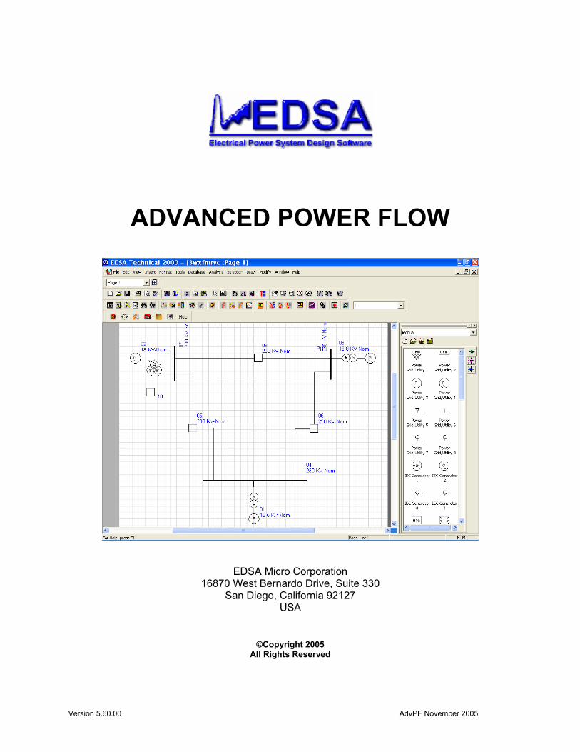
Version 5.60.00 AdvPF November 2005 ADVANCED POWER FLOW EDSA Micro Corporation 16870 West Bernardo Drive, Suite 330 San Diego, California 92127 USA ©Copyright 2005 All Rights Reserved
| Date post: | 29-Oct-2015 |
| Category: |
Documents |
| Upload: | govindarul |
| View: | 43 times |
| Download: | 0 times |
Version 5.60.00 AdvPF November 2005
ADVANCED POWER FLOW
EDSA Micro Corporation 16870 West Bernardo Drive, Suite 330
San Diego, California 92127 USA
©Copyright 2005 All Rights Reserved

Advanced Power Flow
i
Table of Contents
1. What is New in this Release ................................................................................................... 1 2. Program Description and Capabilities .................................................................................... 1 3. Solution Methods .................................................................................................................... 2 4. Generator Modeling ................................................................................................................ 2 5. Under Load Tap Changing Transformers (ULTC)................................................................. 3
Voltage Controlling ULTC ....................................................................................................... 3 Phase Shifting/Active Power Controlling ULTC .................................................................. 4 Reactive Power Controlling ULTC......................................................................................... 4
6. Area Interchange Control........................................................................................................ 4 7. Three Winding Transformers.................................................................................................. 6 8. Autotransformers .................................................................................................................... 6 9. Line Voltage Regulator (LVR) ............................................................................................... 7 10. Motor Starting..................................................................................................................... 8
Motor Starting Using Motor Equivalent Circuit....................................................................... 10 Motor Starting Using Motor Testing Characteristics/SKVA.................................................... 12 Assessing Adequacy of Motor Electrical Torque and Load Torque Curve Fitting .................. 13
11. Power Flow Solution Options and Controls ..................................................................... 15 12. Customizing the EAPF Report, Setting Units and Exporting Facilities ........................... 17 13. Violation and Summary Reports....................................................................................... 21 14. Important Notes ................................................................................................................ 22
Selection of Base Power “BASE MVA/KVA” ........................................................................ 22 What to do if the Load Flow does not converge....................................................................... 22
15. Tutorial: ULTC using Two-Winding Transformers ......................................................... 23 16. Tutorial: ULTC using Three-Winding Transformers ....................................................... 34 17. Tutorial: Voltage Control Using Generators..................................................................... 40 18. Tutorial: Voltage Control Using Static VAR Compensators............................................ 48 19. Tutorial: Advanced Power Flow Based Motor Starting Analysis .................................... 55 20. Tutorial: Area Control....................................................................................................... 67 21. Tutorial: Variable Frequency Motor Starters.................................................................... 74 22. Motor Decrement Export Function from Advanced Motor Starting to Protective Device Coordination.................................................................................................... 85 23. Tutorial: Using DC Lines and Verification and Validation............................................ 100
Verification and Validation of DC Line Model...................................................................... 108 DC Line Sample Network 2.................................................................................................... 108
List of Figures
Figure 1: ULTC Voltage Control Transformer Controlling its Own Terminal or Remote
Bus.......................................................................................................................................... 4 Figure 2: Area Interchange Control ........................................................................................... 5 Figure 3: Schematic of an Autotransformer Circuit................................................................. 7 Figure 4: Line Voltage Regulator (LVR) ................................................................................... 8 Figure 5: General Motor Data Dialog ........................................................................................ 9 Figure 6: Equivalent Circuit Motor Model ............................................................................... 11
Advanced Power Flow
ii
Figure 7: Equivalent Circuit Motor Data Dialog ..................................................................... 12 Figure 8: Defining Motor Characteristics as a Function of Speed...................................... 13 Figure 9: Selecting Electrical Torque Assessment and Load Torque Fitting Option....... 14 Figure 10: Motor Start Testing and Load Torque Curve Fitting .......................................... 15 Figure 11: Advanced Power Flow Solution Options ............................................................. 16 Figure 12: Initializing the Power Flow Solution with Preliminary Gauss-Seidel Iterations
............................................................................................................................................... 16 Figure 13: Representation of the Sources (generator) Impedance During Motor Start.. 17 Figure 14: Setting Report Units in the Advanced Power Flow Program ........................... 18 Figure 15: Selection of Reports, Units, Customizing, and Exporting Power Flow Results
............................................................................................................................................... 18 Figure 16: Exporting the Motor Start Result to Excel ........................................................... 19 Figure 17: Exporting the Motor Start Result to Excel in Actual Values ............................. 20 Figure 18: Exporting the Motor Start Result to Excel in p.u. ............................................... 20 Figure 19: Exporting and Plotting the Motor Start Result in Excel ..................................... 21 Figure 20: Sample Power System used for DC Line Tutorial ........................................... 100 Figure 21: Selecting DC line Symbol .................................................................................... 101 Figure 22: DC Line Data Dialog ............................................................................................. 102 Figure 23: DC Line Data Dialog - Rectifier and Inverter .................................................... 103 Figure 24: Rectifier and Inverter Data................................................................................... 104 Figure 25: Power Flows Shown on the Single Line Diagram of the Sample Network with
DC Line .............................................................................................................................. 106 Figure 26: Example of a Power System using DC Line, “T14bus-dc” ............................. 109 Figure 27: DC Line Data for the Sample Network using DC Line .................................... 110 Note: You can view this manual on your CD as an Adobe Acrobat PDF file. The file name is:
Advanced Power Flow AdvPF.pdf You will find the Test/Job files used in this tutorial in the following location:
C:\EDSA2005\Samples\ADPF = Advanced Power Flow Test Files: 2wxfmrvc, 3wxfmrvc, Advlfv_v, areacont, genvc, motv_v, svcvc, T14bus, T9bus, T9busm, tv_v, T14bus-DC, T9bus-DC
Important Note: The Advanced Power Flow handles long bus ID names up to 24 alphanumeric characters. It is recommended, however that you use 14 characters. If you use more than 18 characters your branch current will have more than one line.
©Copyright 2005 All Rights Reserved

Advanced Power Flow
iii
Page left intentionally blank

Advanced Power Flow
Page: 1
1. What is New in this Release The EDSA Advanced Power Flow (EAPF) program has been enhanced to support full models of DC lines. The DC transmission is the most economical means of power transfer over long distances. It is also used to interconnect power systems asynchronously. There are many DC lines operating in the North American, and European power systems, and more recently planned for the Middle East interconnection. A DC line model is composed of rectifier transformer, rectifier, DC line, inverter, and inverter transformer. The solution process for DC lines in the EDSA Advanced Power Flow program is as follow. The program will attempt to achieve the user specified DC active power flow and DC voltage by first adjusting the rectifier and inverter transformers taps. If this is not successful, then, the program will adjust the rectifier firing angle and inverter extinction angles. The EDSA Advanced Power Flow program utilizes a robust DC solution algorithm with excellent convergence properties. If DC solution does not converge, the user should check any of the following:
The rectifier and inverter transformers are “voltage control” type transformers with sufficient tap ranges
The DC voltage is reasonable (e.g. approximately =1.35*AC voltage * No. of bridges) The firing and extinction angles are reasonable (e.g. 15 and 18 degrees respectively) The desired DC active power is within converter transformer capability The number of bridges are reasonable (e.g. 1, 2, 3, or 4)
The details of DC line model and example of how to use them in a power system are provided in the section 23. 2. Program Description and Capabilities The EDSA Advanced Power Flow program is one of the most powerful, fast, and efficient power flow programs with excellent graphical user interface. EAPF supports advanced plotting, motor starting, numerous options and modeling features. The EAPF program is based on an advanced and robust solution algorithms, which incorporates state-of-the-art solution techniques applicable to large and complex systems. The program is equipped with an easy to use and intelligent graphical interface. The program’s modeling capabilities include: • Generator Local/Remote Bus Voltage Control; • Five solution techniques: Newton-Raphson, Fast De-coupled, Hybrid Solution, Advanced Gauss Seidel,
and Relaxed Generator Reactive Power (Q) limits; • Bus types can be defined as follows: “out of service”, “load”, “generator”, or “Swing Bus”; • Multiple Swing Busses/Co-Generation Units; • Multiple Independent Islands; • Generator models can have different modes of operation: “fixed power output”, “fixed active power &
control voltage at the terminal or at a remote location” • Two and Three-Winding Voltage Control Transformer Models; • Transformers with fixed tap, voltage control, phase shifter (active power control), and reactive power
control; • Transformers can be equipped with Under Load Tap Changers (ULTC) for local and remote bus
voltage control • SVC “Static-Var Compensation” and Shunt capacitor and reactors; • “Area Interchange Control.” Many areas can participate in the area power interchange. Each area will
have a dedicated generator for controlling the tie line power; • DC lines and converter models;

Advanced Power Flow
Page: 2
• Motor starting feature based on IEEE brown book including a variety of the latest solid-state/soft-state motor start controllers;
• No bus-numbering limitations; • Line Voltage Regulator "LVR"; • Unlimited Generators and/or Motors schedules, plus transformer and cable sizing through ADPF
simulation. (Available in the next release of EAPF). The Program output includes: • Bus voltage and angle; • Reactive power, terminal voltage and remotely controlled bus (if any), power factor for generators; • Active, reactive power flows and flow power factor through branches; • Line and total system losses; • Total Generation, Consumption, Losses, and System Mismatch; • Voltage Violations report vs. user-defined threshold; • Line Loading Violations vs. user-defined threshold; In Addition, all of the solution quantities (voltages and flows) are exportable to Excel, and can be used to customize reports using Professional Report Writer. 3. Solution Methods To cope with the unique features of different power systems, such as transmission, distribution and industrial power systems, or a mix of these systems, EAPF supports a number of solution techniques. The solution methods are Newton-Raphson, Fast Decoupled, Hybrid Solution, and the Gauss-Seidel. The latter offers better convergence for the networks having branches with high R/X. This situation may arise especially in a power system with predominately cable installations. The users may select the relaxed Fast Decoupled method when experiencing non-convergence. In this solution technique, transformer taps will not be adjusted and the generators are assumed able to deliver/absorb reactive power beyond their reactive power capabilities. This solution technique is particularly useful when the user wishes to determine the reactive power requirements in a new installation, or sometimes with a power system having data errors. If the Fast-Decoupled method does not converge even when you deactivate the constraints (relaxed solution method), the user should use the Gauss-Seidel method. Since this method is inherently slow in convergence, user should allow more iterations. Hybrid Solution is a very powerful technique suitable when systems with a diverse voltage, load sizes and impedances are modeled. This method utilizes both Newton-Raphson and Gauss-Seidel techniques. The active power mismatch is solved using Newton-Raphson and reactive power mismatch is solved using Gauss-Seidel. 4. Generator Modeling The generator can be modeled using any of the following options:

Advanced Power Flow
Page: 3
• Fixed generation i.e., the user specifies constant active and reactive power generation; • Voltage controlled also referred to as P-V, in this case active power and reactive power capability
(maximum and minimum reactive power) is specified. In addition, the user specifies a desired controlled voltage for either generator terminal or a remote bus. The EAPF solution will determine how much reactive power is required to maintain the desired controlled voltage;
• Swing generator (sometimes it is also referred to as Utility or Reference generator). In this case, the user only specifies desired controlled voltage and its voltage angle (normally set to zero) at the generator terminal. EAPF will determine the required active and reactive power generation at the swing generator.
The user may connect more than one generator to a bus. The generators do not have to be the same rating and type. The following explains how EAPF divides the power among generators connected at the same bus: • Fixed generators do not participate in the allocation; • Swing generators share the required active and reactive generation equally; • Voltage-controlled generators when each produces its specified active generation. Their share of
the reactive power required in the solution is distributed proportionately to their reactive power capability range (without violating their limit).
5. Under Load Tap Changing Transformers (ULTC) The EAPF program supports three types of ULTC transformers, which are described in the following section: Voltage Controlling ULTC This transformer can be used to control the voltage at either side of the transformer, or alternatively, it may control the voltage at the bus remote from the transformer terminals. For the latter case, to be practical, the remote bus should be in close proximity of the transformer. The required input data are: • Transformer leakage impedance and ratings; • Available tap range, maximum and minimum tap and number of taps; • The range of controlled voltage (maximum and minimum voltage); • The controlled bus identification. This may be either one of the transformer’s terminals or a valid
remote bus in the network. For example, in Figure 1, a voltage regulating ULTC is connected between buses: BUSA and BUSB. The transformer tap can be on BUSA or BUSB and the voltage may be controlled at BUSA or BUSB or a remote bus such as BUSC. The power flow program will adjust the transformer tap to maintain the voltage at the controlled bus between the maximum and minimum specified voltage. In cases where the program is unable to control the voltage within the specified range, the transformer tap will be at either

Advanced Power Flow
Page: 4
Figure 1: ULTC Voltage Control Transformer Controlling its Own Terminal or Remote Bus
minimum or maximum tap position. The position is also user defined and can be either one of the transformer’s terminals. Phase Shifting/Active Power Controlling ULTC This type of transformer can be used to control the flow of active power through the transformer. It is also known as phase shifting transformer. The required input data are: • Transformer leakage impedance and rating; • Available phase shift range (maximum and minimum phase shift and number of taps); • The range of controlled active power through the transformer. The EAPF program will automatically adjust the transformer phase shift within its controlled range until the desired active power flow through transformer is obtained. If unable to control active power flow to the prescribed value, the phase shift will be set at either maximum or minimum allowable values. Reactive Power Controlling ULTC. This transformer controls the flow of reactive power flow trough the transformer by adjusting its tap. The required input data are: • Transformer leakage impedance and ratings; • Available tap range (maximum and minimum tap and number of taps); • The range of controlled reactive power flow through transformer; The EAPF program will automatically adjust the transformer tap within its controlled range until the desired reactive power through transformer is obtained. If unable to control reactive power flow to the prescribed values, the transformer tap will be set at either maximum or minimum allowable values. 6. Area Interchange Control This modeling of EAPF program can be used to simulate power transactions between utilities or areas of a power network. To illustrate this modeling concept, consider the following example based on Figure 2:
Figure 1

Advanced Power Flow
Page: 5
Let’s assume that there are three areas in the network, as shown in the figure. Area 2 is exporting power to areas 1 and 3. Area 1 is only importing power from areas 2 and 3. However, area 3 is both importing and exporting power to areas 1 and 2. The following data are the required for each area:
Figure 2: Area Interchange Control
• Area name; • Bus identification of the area control generator; • Net exchange value of Active Power. This number could be positive or negative. If the exchange is
positive, then, it is considered to be exporting power. • Tolerance of MW Exchange; • Maximum and Minimum active generation of the area control generator; • “Zones” per “Area” assignment, many zones can be assigned to one area. Tie lines are branches that link system areas and are entered like any other lines. The metering point for a tie line is the "From bus". Losses on the tie line are accounted for in the area of the "To bus". The power flow program automatically determines (using network connectivity information and zones in areas) the associated area tie lines. For example, in Figure 2, there is one tie line between area 1 and area 2. There are three tie lines between areas 3 and 1 and finally two tie lines between areas 2 and 3. For each iteration the program will try to adjust the area control active power generation (within its specified maximum and minimum) such that the desired amount of import and export within each area is achieved. Note that each area should have unique zones assigned to it. For example if there are 10 zones, then: Area 1 can have zones 3,5,9. Area 2 can have 1,2,7 Area 3 can have 4,6,8 and 10
Area 1
Area 2
Area 3
Area Control Generato r
Area Control Generato r
Area Control Generator
Figure 2
Advanced Power Flow
Page: 6
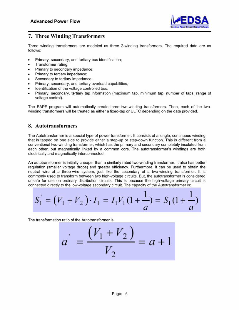
7. Three Winding Transformers Three winding transformers are modeled as three 2-winding transformers. The required data are as follows: • Primary, secondary, and tertiary bus identification; • Transformer rating; • Primary to secondary impedance; • Primary to tertiary impedance; • Secondary to tertiary impedance; • Primary, secondary, and tertiary overload capabilities; • Identification of the voltage controlled bus; • Primary, secondary, tertiary tap information (maximum tap, minimum tap, number of taps, range of
voltage control). The EAPF program will automatically create three two-winding transformers. Then, each of the two-winding transformers will be treated as either a fixed-tap or ULTC depending on the data provided. 8. Autotransformers The Autotransformer is a special type of power transformer. It consists of a single, continuous winding that is tapped on one side to provide either a step-up or step-down function. This is different from a conventional two-winding transformer, which has the primary and secondary completely insulated from each other, but magnetically linked by a common core. The autotransformer’s windings are both electrically and magnetically interconnected. An autotransformer is initially cheaper than a similarly rated two-winding transformer. It also has better regulation (smaller voltage drops) and greater efficiency. Furthermore, it can be used to obtain the neutral wire of a three-wire system, just like the secondary of a two-winding transformer. It is commonly used to transform between two high-voltage circuits. But, the autotransformer is considered unsafe for use on ordinary distribution circuits. This is because the high-voltage primary circuit is connected directly to the low-voltage secondary circuit. The capacity of the Autotransformer is:
The transformation ratio of the Autotransformer is:

Advanced Power Flow
Page: 7
Figure 3: Schematic of an Autotransformer Circuit
For example, if a=1, the capacity has been doubled! The advantages of autotransformers include:
No “galvanic” isolation between primary and secondary windings; More power transformation capacity with the same size of the transformer; Possibilities to control voltage and reactive power flow; Widespread applications in power systems.
The mathematical model of an autotransformer is similar to a two-winding transformer and the EAPF treats an autotransformer the same as a voltage-controlled transformer but with simplified data requirements.
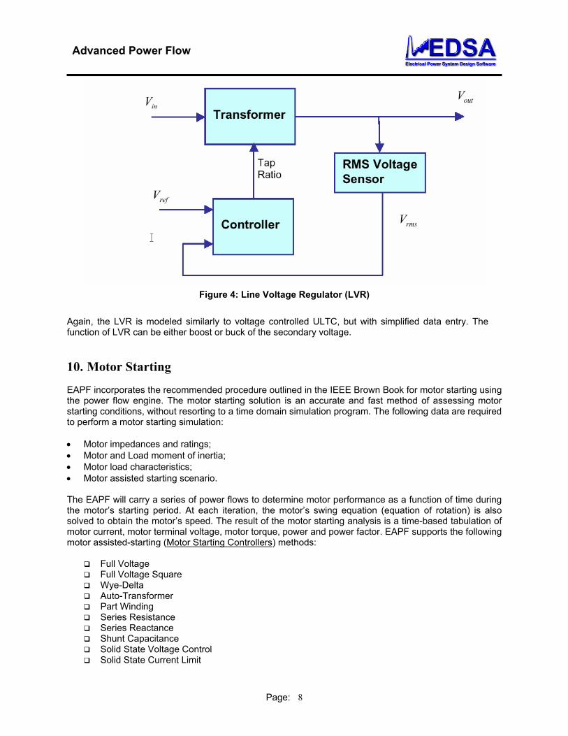
9. Line Voltage Regulator (LVR) The line voltage regulator normally uses several-tap autotransformer to control the voltage to a precise set point. The Voltage Regulator circuitry monitors the incoming line voltage and compares it to a voltage reference set point. If a voltage fluctuation requires that a different tap be selected, the new tap is electronically switched (normally at the zero-crossing, to avoid distorting the AC waveform). In some design, if necessary, it can switch taps as often as once each cycle. Most commercial voltage regulators using multiple-tapped transformers switch taps at uncontrolled times, thereby creating voltage spikes.
Advanced Power Flow
Page: 8
Figure 4: Line Voltage Regulator (LVR)
Again, the LVR is modeled similarly to voltage controlled ULTC, but with simplified data entry. The function of LVR can be either boost or buck of the secondary voltage. 10. Motor Starting EAPF incorporates the recommended procedure outlined in the IEEE Brown Book for motor starting using the power flow engine. The motor starting solution is an accurate and fast method of assessing motor starting conditions, without resorting to a time domain simulation program. The following data are required to perform a motor starting simulation: • Motor impedances and ratings; • Motor and Load moment of inertia; • Motor load characteristics; • Motor assisted starting scenario. The EAPF will carry a series of power flows to determine motor performance as a function of time during the motor’s starting period. At each iteration, the motor’s swing equation (equation of rotation) is also solved to obtain the motor’s speed. The result of the motor starting analysis is a time-based tabulation of motor current, motor terminal voltage, motor torque, power and power factor. EAPF supports the following motor assisted-starting (Motor Starting Controllers) methods:
Full Voltage Full Voltage Square Wye-Delta Auto-Transformer Part Winding Series Resistance Series Reactance Shunt Capacitance Solid State Voltage Control Solid State Current Limit
Advanced Power Flow
Page: 9
Solid State Current Ramp Solid State Voltage Ramp Solid State Torque Ramp Variable Frequency Drive
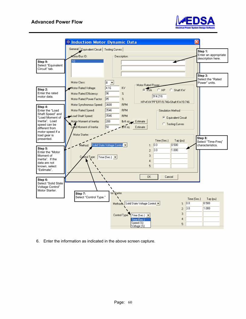
The above motor assisted-starting options cover a wide variety of the recent solid-state motor starting controls as well as the most traditionally used starting methods. The main objective behind the use of assisted-starting methods is to control (limit) the impact of motor starting events on the electrical power systems. Data requirements for each of the above motor assist starting options are described in the user’s manual. For example, the data and functionality of the “Solid State Voltage Control” are summarized in Figure 5, page 9. This figure shows the EAPF screen corresponding to input data for motor starting. The “Control Type” can be set to any of the following options: time, speed or motor bus voltage. This is seen in the lower part of the screen capture. In this example, at bus 10 there is a motor to be started, motor 10. Time is selected to be control type. The user also needs to input rated voltage (KV), rated efficiency (%), rated power factor (%), synchronous speed (RPM), etc. as shown. The moment of inertia can be entered or estimated.
Step 1: Enter an appropriate description here.
Step 2: Enter the rated motor data.
Step 3: Select the “Rated Power” units.
Step 5: Enter the “Motor Moment of Inertia”. If the data are not known, select “Estimate”.
Step 6: Select “Solid State Voltage Control” Motor Starter.
Step 7: Select “Control Type.”
Step 8: Select “Time-Freq” characteristics.
Step 9: Select “Equivalent Circuit” tab.
Step 4: Enter the “Load Shaft Speed” and “Load Moment of Inertia”. Load speed can be different from motor speed if a load gear is presented.
Figure 5: General Motor Data Dialog

Advanced Power Flow
Page: 10
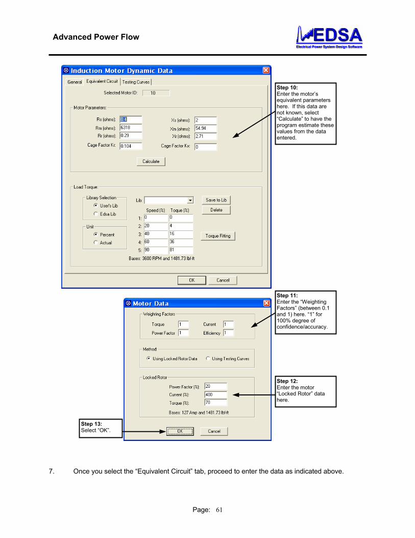
Other motor data as shown in Figure 5 above, include: • full load speed, (RPM); • motor rated power, in KVA, HP or shaft KW; • motor class. A, B, C, or D. As it can be seen, the program allows the user to specify or calculate the motor design class according to NEMA conventions. NEMA classifies induction motors according to the following categories, which are based on the ratio of X1 to X2 (X1/X2): • Class A X1/X2 = 1 • Class B X1/X2 = 2/3 • Class C X1/X2 = 3/7 The EDSA induction motor parameter estimation provides four options: • Class A applies to: User defined NEMA class A • Class B applies to: User defined NEMA class B • Class C applies to: User defined NEMA class C • Class D applies to: User defined as NEMA class “ not known”. When class D is selected, the program
will automatically determine the motor’s NEMA class based on the data provided by the user. In the “Equivalent Circuit” tab the user can enter the motor parameters and load torque (in per cent or actual units). The user should enter the motor’s equivalent electrical parameters; if this data are not known, then the user selects “Calculate” button, and the program calculates the motor parameter based on starting information and weighting factors. The weighting factors can be assigned for the following motor parameters: • Current, • Torque, • Power Factor, • Efficiency. A weighting factor applied to any of the above parameters is a number between 0.1 and 1. This number represents the degree of confidence the user has on the accuracy of the particular figure being entered. The program offers full automatic on-screen conversion between the different power units. In addition to the above basic input data, the user may specify a number of operating points – motor characteristics, as a function of speed. The sample points provided by the user can be sparse, in other words, the user does not need to have all the data for all the included operating points. For example, at speed zero (slip=1) the user may have the knowledge of the motor power factor and starting current but not of the electrical torque and efficiency. Motor Starting Using Motor Equivalent Circuit The motor starting analysis can be performed by using either motor equivalent circuit impedances (rotor and stator), or the motor characteristics (current, torque, etc.) at different speeds. In the former case, the user should provide the rotor and stator impedances as shown in Figure 7. If the impedances are not known then, the user may use the induction motor parameters estimation program by choosing the “Calculate” button shown in Figure 7.

Advanced Power Flow
Page: 11
The Equivalent circuit of the motor is shown in Figure 6. The power flow program computes the motor
equivalent impedance based on: 11
22
22
)()(
*)]()([jXR
jXsjXs
sR
jXsjXs
sR
Zm
m
mot ++++
+=
Figure 6: Equivalent Circuit Motor Model
The motor equivalent impedance (recall that rotor resistance and reactance are assumed to be function of speed according to cage factors defined) is then placed at the motor bus similar to a shunt and power flow is solved. At every power flow solution, the motor rotational equation (also referred to as swing equation) shown below is also solved to compute the subsequent motor speed in time.
me TTdtdwH −=**2

Advanced Power Flow
Page: 12
Step 10: Enter the motor’s equivalent parameters here. If this data are not known, select “Calculate” to have the program estimate these values from the data entered.
Step 11: Enter the “Weighting Factors” (between 0.1 and 1) here. “1” for 100% degree of confidence/accuracy.
Step 12: Enter the motor “Locked Rotor” data here.
Step 13: Select “OK”.
Figure 7: Equivalent Circuit Motor Data Dialog
Motor Starting Using Motor Testing Characteristics/SKVA The power flow program also supports the motor starting using the motor characteristics provided at different speed intervals (this is also known as SKVA method). These characteristics are kVA, power factor, electrical and load torques as shown in Figure 8 and are normally provided by the motor manufacturer from either field-testing or via mathematical motor modeling. The user may specify up to 100 points of data and save the characteristics into the library, or retrieve the data points from the library.

Advanced Power Flow
Page: 13
Figure 8: Defining Motor Characteristics as a Function of Speed
The power flow program will not attempt to compute the individual motor impedances (rotor and stator) in this method, but rather will compute the total equivalent impedance from the kVA and power factor information. The electrical torque and kVA are of course adjusted according to:
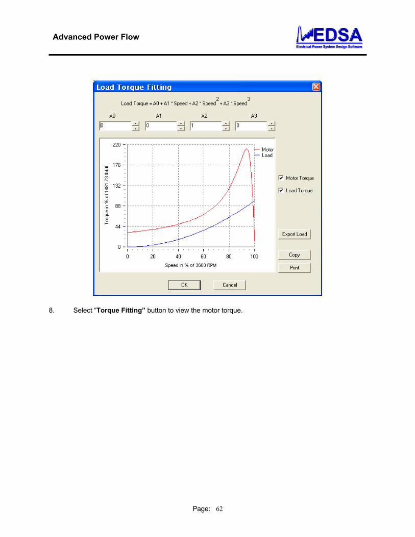
2*)( VgivenTT ee = VgivenkVAkVA *)(= Assessing Adequacy of Motor Electrical Torque and Load Torque Curve Fitting The EAPF allows the user to quickly assess the electrical torque that the motor can develop from the motor data provided. This feature facilitates the selection of a particular motor design based on the load torque requirements. The program takes into account any motor starter that the user has specified or alternatively, performs the analysis for full voltage start. For example, in the screen below, the data for

Advanced Power Flow
Page: 14
one induction motor have been specified and starter type of “Variable Frequency Drive” has been defined. To see the developed electrical torque select “Torque Fitting” as shown in Figure 9.
Figure 9: Selecting Electrical Torque Assessment and Load Torque Fitting Option
The EAPF program, then, quickly performs the motor starting and displays the result of electrical torque and load torque as shown in Figure 10. The load torque can be adjusted by changing the coefficients A0-A3. To examine electrical torque for different motor parameters, modify the motor impedances shown in Figure 9 and repeat the same process again until the desired performance is achieved.

Advanced Power Flow
Page: 15
Figure 10: Motor Start Testing and Load Torque Curve Fitting
11. Power Flow Solution Options and Controls The EAPF program solution options and control parameters are shown in Figure 11. With these options user can select:
Solution Method (Newton, Gauss, etc.); Convergence tolerance; Select Automatic Adjustments (ULTC’s, Generator, and SVC); Source (Generator) Impedance Representation For Motor Start; Zero Impedance Branch Threshold;
The solution options were described in the previous sections. EAPF also allows the user to initialize the power flow solution by Gauss-Seidel method. This is shown in Figure 12 where the number of initial iteration is specified as 20.
Advanced Power Flow
Page: 16
Figure 11: Advanced Power Flow Solution Options
Figure 12: Initializing the Power Flow Solution with Preliminary Gauss-Seidel Iterations
The EAPF program supports representation of generator impedance during motor starting. The user may select to represent sub-transient, transient, or the average value of the sub-transient and transient impedances. If the generator impedance is to be taken into account, the EAPF computes the internal voltage of the generator (voltage behind its impedance) from the initial power flow solution and then sets the internal voltage to be the swing bus as shown in Figure 13:

Advanced Power Flow
Page: 17
Figure 13: Representation of the Sources (generator) Impedance During Motor Start
The above representation is very realistic and results in higher voltage drop and longer motor start up time. The EAPF program will use “Branch Impedance Threshold”, also referred to Zero Impedance Line (ZIL), to eliminate any branch (cable or line) the impedance is smaller than ZIL from the network solution. This option will be active and explained in the next release of the EAPF. 12. Customizing the EAPF Report, Setting Units and Exporting Facilities The EAPF supports a number of standard reports that are commonly accepted by the power industry load flow report formats. In addition to these reports, the result of power flow solution, i.e., voltages and power flows can be exported to Excel program. The reports can also be customized by advance “Professional Report Writer Wizard”. The units for reporting voltages and flows can be selected as shown in Figure 14. The voltages can be reported in p.u, volts, or kV. The unit of current report can be p.u., Amps, or kA. Finally, the active and reactive powers are reported in p.u., KW/KVAR, or MW/MVAR.

Advanced Power Flow
Page: 18
Figure 14: Setting Report Units in the Advanced Power Flow Program
Figure 15 shows how different report options can be accessed in the Advanced Power Flow Program.
Figure 15: Selection of Reports, Units, Customizing, and Exporting Power Flow Results
Advanced Power Flow
Page: 19
For example, when “Export Result to Excel” for motor starting reports is selected, the program will prompt the user to assign a file name as shown in Figure 16:
Figure 16: Exporting the Motor Start Result to Excel

Advanced Power Flow
Page: 20
Figure 17 shows the results of exporting motor start results Excel from Advanced Power Flow Program. It can be seen that the results are exported (in this case) in actual values.
Figure 17: Exporting the Motor Start Result to Excel in Actual Values
Figure 18 shows the results of a motor start analysis when exported to Excel from Advanced Power Flow Program. In this case the results are reported in p.u.
Figure 18: Exporting the Motor Start Result to Excel in p.u.

Advanced Power Flow
Page: 21
Finally, to quickly plot the result in Excel program, select the variables of interest as shown in Figure 18 (in this case we have selected “Time” and “Current”). Then, select “Chart Wizard” and follow the process of selecting other graph options. The graph produced by Excel is shown below in Figure 19:
Figure 19: Exporting and Plotting the Motor Start Result in Excel
13. Violation and Summary Reports The violation report identifies undesirable conditions in the network (overloaded equipment and unacceptably high or low voltages). It contains only those transformers, lines and cables that are loaded beyond the limits specified by the user. It also lists only those buses whose voltages fall outside the user-defined acceptable range. The program allows the user to adjust these limits before or even after the load flow calculation. The summary report provides totals of generation, load, losses and mismatches1 in the network. (Losses are the difference between generation and load.) Active and reactive quantities are listed separately. Motor load and static load are identified by separate totals. The solution method, base power, calculation tolerance and mismatches are also listed. The Area Interchange report will also be included in the Summary report if the area interchange option has been selected. It is possible to show the power flows and the bus voltages directly on the one-line diagram.
1 If reported mismatches are not small as compared to the other quantities reported (for example a few percent of the total system load), consider running the load flow again with a smaller tolerance.

Advanced Power Flow
Page: 22
14. Important Notes Selection of Base Power “BASE MVA/KVA” This is the common power base to which all impedances will be referred (per unitized). Choose a value midway between the largest and smallest power rating of the equipment in the network. Convenient values are 0.1, 1, 10 or 100 MVA. What to do if the Load Flow does not converge EAPF generates a file named “ErrorLog”, where all the warnings and error messages are logged. The power flow iterations are also reported in this file. Log file gives the user the information about the convergence of the power flow solution process. Also, if the power system component data are in error, the program will issue messages related to the erroneous data. If the ErrorLog shows that the calculation does not converge, inspect to see what buses have high power mismatches. If from iteration to iteration, the mismatches increase steadily, check the input data for components connected to the indicated buses. Look for very high or very low line/cable/transformer impedances. Make sure line and cable lengths are consistent with the length unit used for defining the impedance. If the mismatches increase and decrease and devices are being adjusted on every iteration, try solving without constraints. If that calculation converges, you may be able to see from the results what is wrong. Perhaps two devices have been asked to control the voltage at the same bus. If the convergence seems to be going up and down, this is an indication that some transformers/generators devices are continually being adjusted. If so, you may also try changing the settings of one or more of these devices before re-attempting another run. If the mismatches steadily decrease but remain higher than the specified tolerance as the permitted number of iterations is exhausted, try increasing the number of iterations before solving again.
Advanced Power Flow
Page: 23
15. Tutorial: ULTC using Two-Winding Transformers
1. Invoke the EDSAT2K Graphical Interface, and proceed to open the file called “2WXFMRVC” as indicated in the above screen capture.

Advanced Power Flow
Page: 24
2. Next, proceed to designate the desired transformer, or transformers, that will be used as ULTC Control Transformers. Follow the instructions shown in the next screen capture.
To invoke the Advance Power Flow Tools toolbar, click here.
Motor Dynamic Information
Area Power Control Options
Advanced Power Flow Options
Analyze
Report Manager
Display Options for Load Flow
Overview – EDSA Toolbar

Advanced Power Flow
Page: 25
3. Proceed to enter the transformer data as well as the Auto Tap Adjustment Control options for this unit. In this example, the type of control will be defined as follows:
Control Variable: Voltage Controlled Bus: FFF69 (69kV Primary Bus) Follow the instructions shown in the above screen capture. Repeat this procedure for as many
transformers as necessary. In this example, only one transformer will be equipped with adjustable taps.
Note: There is no limit in Voltage Control Transformers.

Advanced Power Flow
Page: 26
Step 1. Select the Advanced Power Flow Tools Icon.
Step 2. Proceed to select Advanced Power Flow Options.
4. Next, proceed to invoke the Advanced Power Flow Program, as indicated in the above screen capture.
You will then see the Advanced Power Flow Options screen appear.
Step 1
Step 3
Step 4
Step 2
5. Select Advanced Power Flow Options shown above, then click “OK”.

Advanced Power Flow
Page: 27
- Please review and examine all the options. In this interface you can select Solution Algorithm and Perform Motor Starting. Make sure Motor Starting is Off if performing only Load Flow. You may also turn the Automatic Voltage Control On or Off. You may also turn the Relax Generator Q Limit On or Off. Under the Power Flow Options menu, the user can select the Power Flow Method: Fast Decoupled, Newton Raphson, Hybrid Solution (half Newton Raphson and half Gauss Seidel) or Gauss Seidel. Each of the method employed, can be used with or without relaxing the generator reactive power. Relaxing the generator reactive power is particularly useful when the user wishes to determine reactive power requirements in new installation or sometimes with power system having data errors. The Gauss-Seidel or Hybrid methods are recommended for the networks that have branches with high R/X (cables). This situation may arise especially in a power system with predominately cable installations. The convergence of the Seidel-Gauss iteration algorithm is asymptotic. The users may select the relaxed NEWTON-RAPHSON Fast Decoupled method, when experiencing non-convergence by using Gauss Seidel. The following guidelines are offered as an aid to determine which technique may be the most appropriate for a particular system condition: • The Gauss-Seidel method is generally tolerant of power system operating conditions involving poor
voltage distribution and difficulties with generator reactive power allocation, but does not converge well in situations where real power transfers are close to the limits of the system;
• The Gauss-Seidel method is quite tolerant of poor starting voltages estimates but converges slowly as the voltage estimate gets close to the true solution;
• The Gauss-Seidel method will not converge if negative reactance branches are present in the network, such as due to series capacitors or three-winding transformer models;
• The Newton Raphson method is generally tolerant of power system situations in which there are difficulties in transferring real power, but is prone to failure if there are difficulties in the allocation of generator reactive power output or if the solution has a particularly low voltage magnitude profile; in this situation, it is recommended to select “Relax Generator Reactive Power Limits” option;
• The Newton Raphson method is prone to failure if given a poor starting voltage estimate, but is usually superior to the Seidel-Gauss method once the voltage solution has been brought close to the true solution;
• The Fast Decoupled Newton method will not converge when the network contains lines with resistance close to, or greater than, the reactance (cables). This is often the case in low-voltage systems.
Some experimentation is recommended to determine the best combination of methods for each particular model. The followings are recommended: • Start with Gauss-Seidel (20 iterations); • Switch to Newton- Raphson method until either the problem is converged or Relax Generator
Reactive Power Limits; • Switch back to Gauss-Seidel method if the Newton- Raphson method does not settle down to a
smooth convergence within 8 to 10 iterations. • The Hybrid Solution technique can be used for systems that have diverse voltages, e.g., 400kV to
120v, very high or low impedance mixes and diverse loads, such as, 50HP and 5000HP. This is a very exact, fast, technique for large power distribution and transmission systems.
Advanced Power Flow
Page: 28
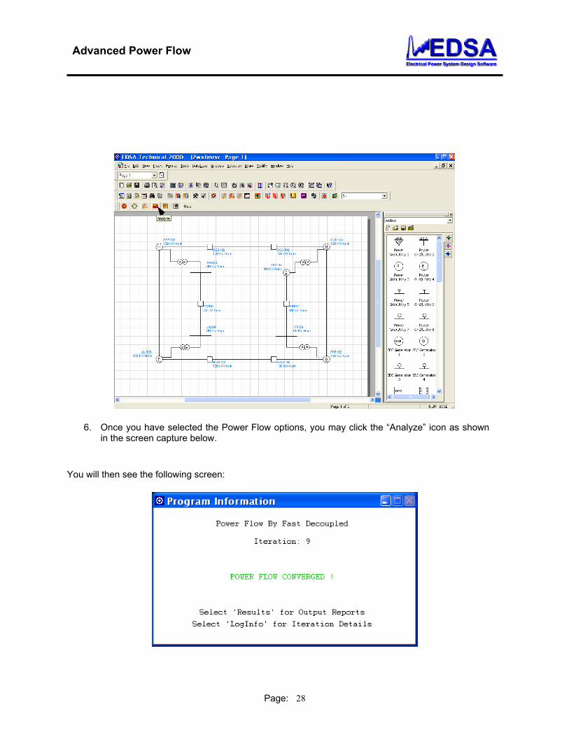
6. Once you have selected the Power Flow options, you may click the “Analyze” icon as shown in the screen capture below.
You will then see the following screen:
Advanced Power Flow
Page: 29
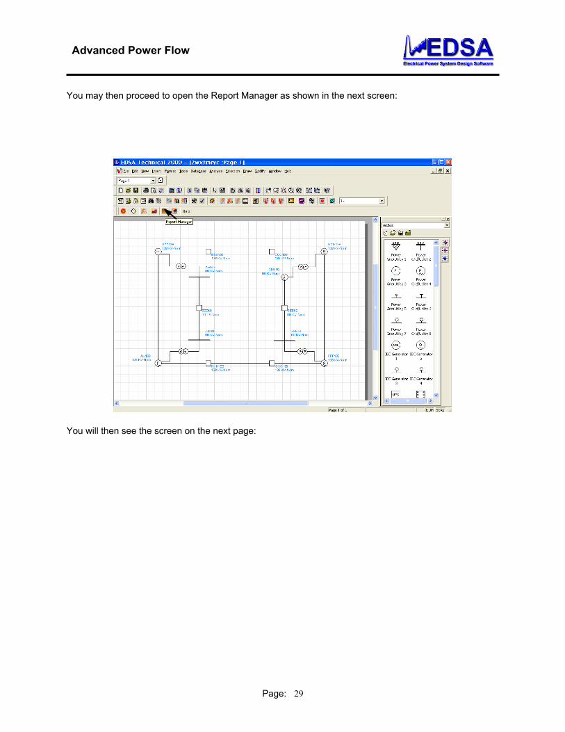
You may then proceed to open the Report Manager as shown in the next screen:
You will then see the screen on the next page:
Advanced Power Flow
Page: 30
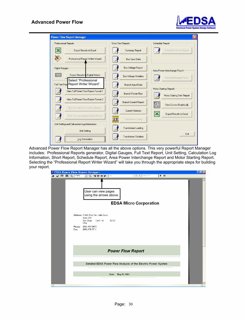
Advanced Power Flow Report Manager has all the above options. This very powerful Report Manager includes: Professional Reports generator, Digital Gauges, Full Text Report, Unit Setting, Calculation Log Information, Short Report, Schedule Report, Area Power Interchange Report and Motor Starting Report. Selecting the “Professional Report Writer Wizard” will take you through the appropriate steps for building your report.
Select “Professional Report Writer Wizard”.
User can view pages using the arrows above.

Advanced Power Flow
Page: 31
The user can view Digital Gauges by selecting “Output Results to Digital Meters”.
Please try all the options and view the outputs.
Sample Bus Digital Meters
Select “Output Results to Digital Meters”.
Select “Buses”.
User can view “All” or select “Buses with Violations” and specify limits.
Advanced Power Flow
Page: 32
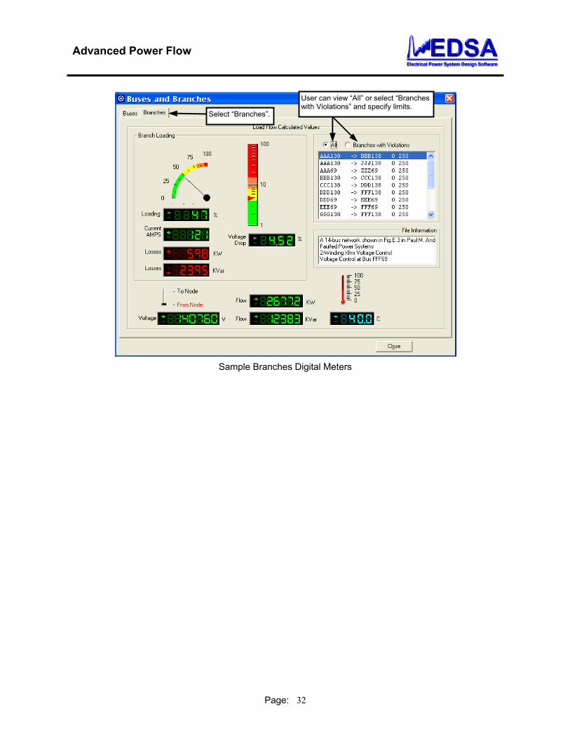
User can view “All” or select “Branches
with Violations” and specify limits. Select “Branches”.
Sample Branches Digital Meters

Advanced Power Flow
Page: 33
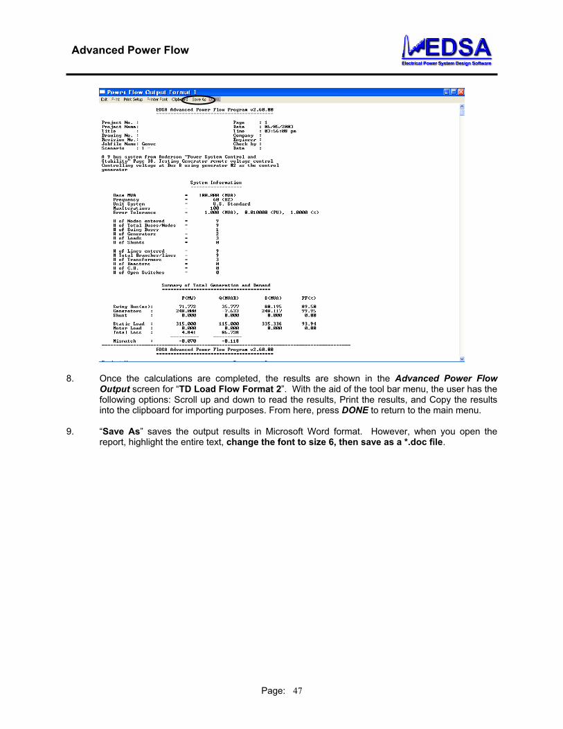
7. Once the calculations are completed, the results are shown in the Advanced Power Flow
Output screen for “TD Load Flow Format 2”. With the aid of the tool bar menu, the user has the following options: Scroll up and down to read the results, Print the results, and Copy the results into the clipboard for importing purposes. From here, press DONE to return to the main menu.
8. “Save As” saves the output results in Microsoft Word format. However, when you open the
report, highlight the entire text, change the font to size 6, then save as a *.doc file.
Advanced Power Flow
Page: 34
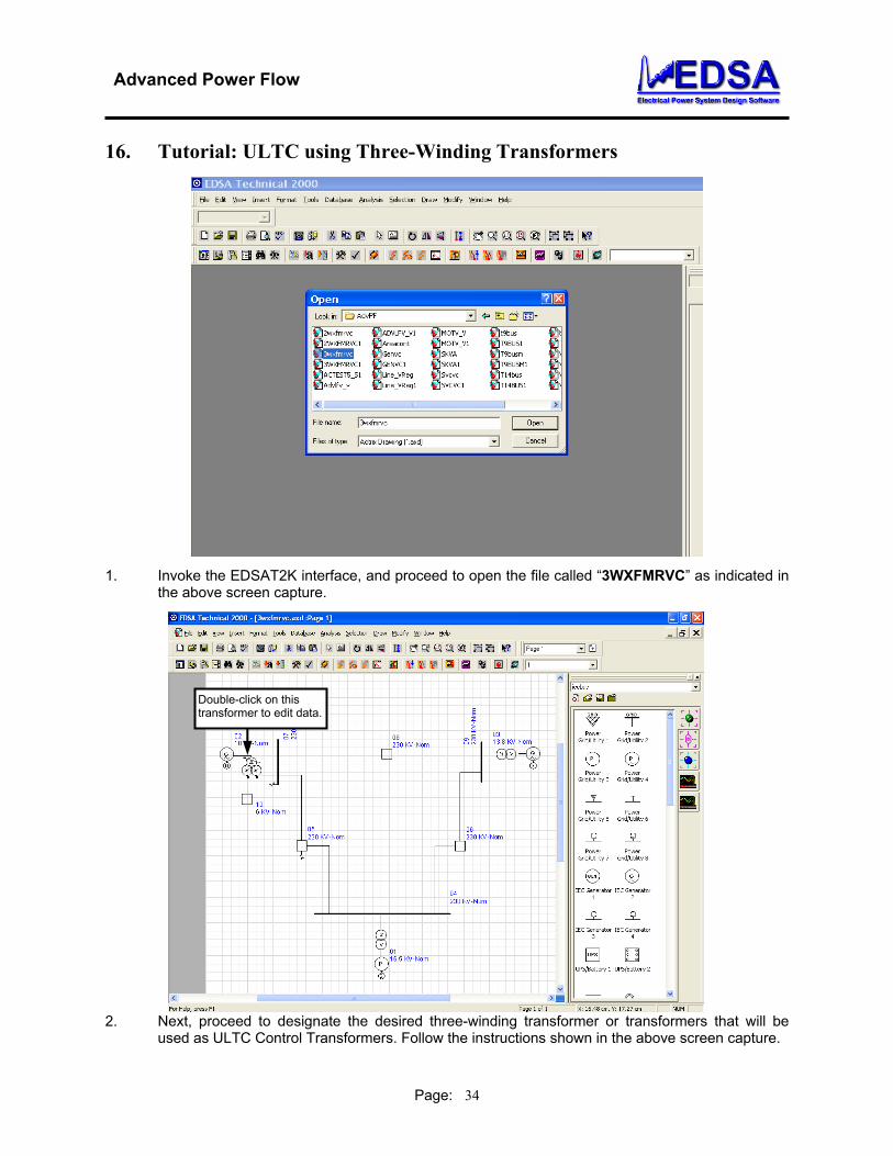
16. Tutorial: ULTC using Three-Winding Transformers
1. Invoke the EDSAT2K interface, and proceed to open the file called “3WXFMRVC” as indicated in the above screen capture.
Double-click on this transformer to edit data.
2. Next, proceed to designate the desired three-winding transformer or transformers that will be
used as ULTC Control Transformers. Follow the instructions shown in the above screen capture.

Advanced Power Flow
Page: 35
3. Proceed to enter the transformer data as well as the Auto Tap Adjustment Control options for this unit. In this example, the type of control will be defined as follows:
Control Variable: Voltage Winding with Taps: Primary and Tertiary Controlled Busses: By Primary > Bus 07 By Tertiary > Bus 10 Follow the instructions shown in the above screen capture. Repeat this procedure for as many
transformers as necessary. In this example, only one transformer will be equipped with adjustable taps.
Advanced Power Flow
Page: 36
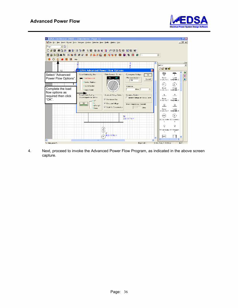
Select “Advanced Power Flow Options”.
Complete the load flow options as required then click “OK”.
4. Next, proceed to invoke the Advanced Power Flow Program, as indicated in the above screen capture.

Advanced Power Flow
Page: 37
Next, select “Analyze”.
Verify that the analysis has converged.
5. Run the analysis by following the instructions shown in the above screen capture.

Advanced Power Flow
Page: 38
Select “Report Manager”.
Next, select “View Full Power Flow Report Format 1”.
6. Next proceed to view the text output results by following the steps in the above screen capture.

Advanced Power Flow
Page: 39
7. Once the calculations are completed, the results are shown in the Advanced Power Flow Output screen for “TD Load Flow Format 2”. With the aid of the tool bar menu, the user has the following options: Scroll up and down to read the results, Print the results, and Copy the results into the clipboard for importing purposes. From here, press DONE to return to the main menu.
8. “Save As” saves the output results in Microsoft Word format. However, when you open the
report, highlight the entire text, change the font to size 6, then save as a *.doc file.

Advanced Power Flow
Page: 40
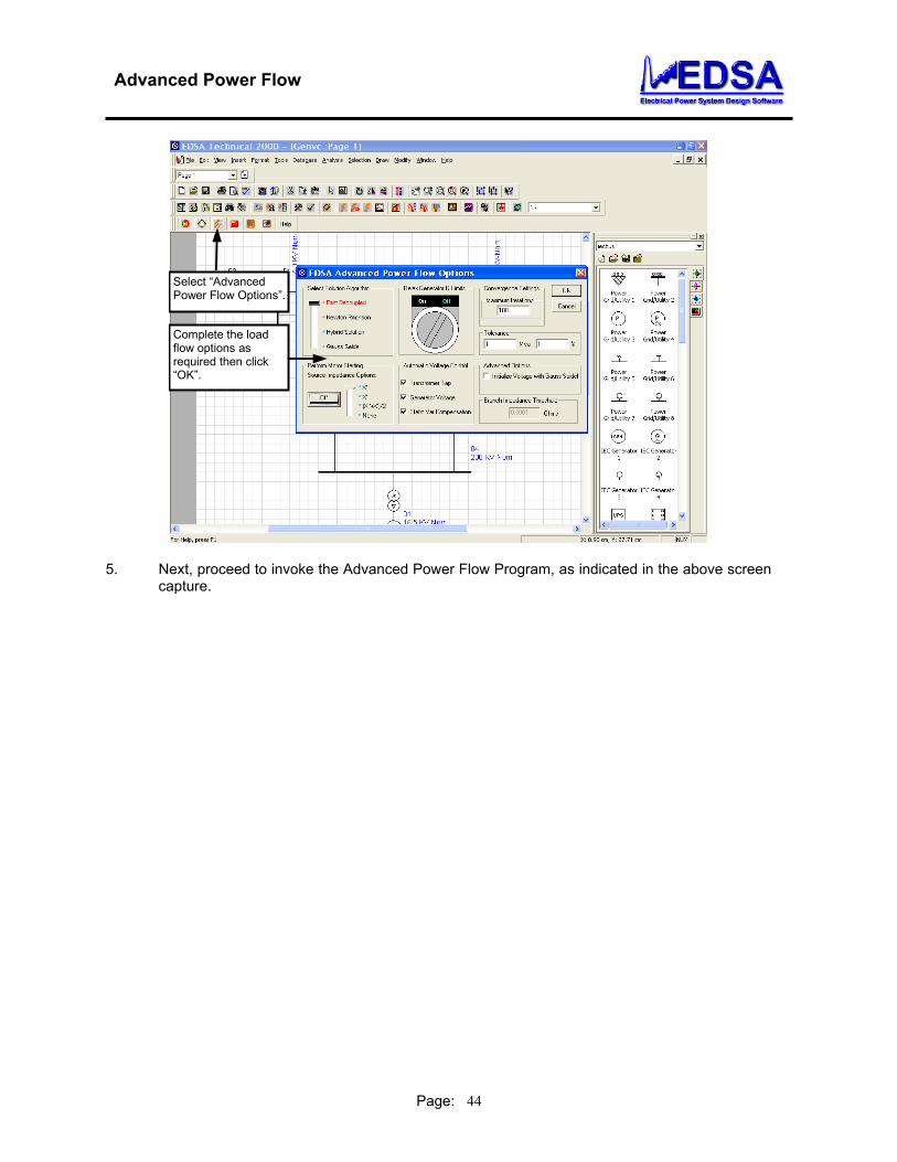
17. Tutorial: Voltage Control Using Generators
1. Invoke the EDSAT2K interface, and proceed to open the file called “GENVC” as indicated in the above screen capture.

Advanced Power Flow
Page: 41
Double-click on the Generators 2 & 3 to complete their respective editors as indicated in step 4.3
2. Next, proceed to designate Generators 2 & 3 as Voltage Control units. Follow the instructions shown in the above screen capture.

Advanced Power Flow
Page: 42
3. Proceed to enter the required data for Generator 2 as indicated in the above screen capture.

Advanced Power Flow
Page: 43
4. Proceed to enter the required data for Generator 3 as indicated in the above screen capture. In those two examples, the type of control will be defined as follows:
Generator 2: Controlled Bus: 08
Desired Voltage: 1.00 PU Generator 3: Controlled Bus: 03
Desired Voltage: 1.02 PU
Repeat this procedure for as many generators as necessary. In this example, only two generators will be used for voltage control.
Advanced Power Flow
Page: 44
Select “Advanced Power Flow Options”.
Complete the load flow options as required then click “OK”.
5. Next, proceed to invoke the Advanced Power Flow Program, as indicated in the above screen capture.

Advanced Power Flow
Page: 45
Next, select “Analyze”.
Verify that the analysis has converged.
6. Run the analysis by following the instructions shown in the above screen capture.

Advanced Power Flow
Page: 46
Select “Report Manager”.
Next, select “View Full Power Flow Report Format 1”.
7. Once the calculations have been completed, proceed to view the output report as indicated in the above screen capture.
Advanced Power Flow
Page: 47
8. Once the calculations are completed, the results are shown in the Advanced Power Flow Output screen for “TD Load Flow Format 2”. With the aid of the tool bar menu, the user has the following options: Scroll up and down to read the results, Print the results, and Copy the results into the clipboard for importing purposes. From here, press DONE to return to the main menu.
9. “Save As” saves the output results in Microsoft Word format. However, when you open the
report, highlight the entire text, change the font to size 6, then save as a *.doc file.
Advanced Power Flow
Page: 48
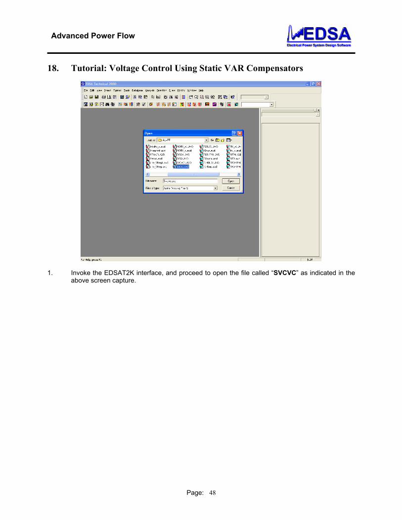
18. Tutorial: Voltage Control Using Static VAR Compensators
1. Invoke the EDSAT2K interface, and proceed to open the file called “SVCVC” as indicated in the above screen capture.

Advanced Power Flow
Page: 49
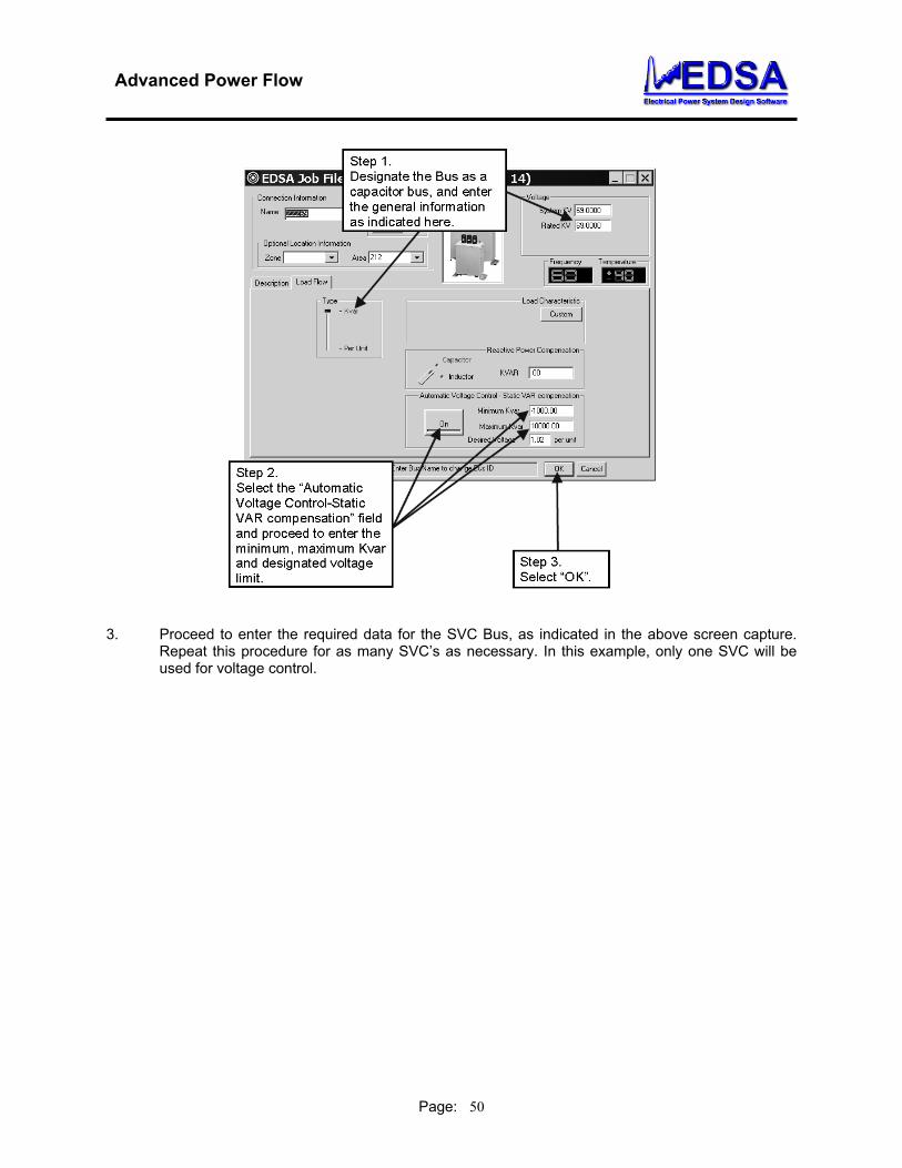
Double-click on this Bus to edit data.
2. Next, proceed to designate Bus ZZZ69 as a Static VAR Compensation Bus. Follow the instructions shown in the above screen capture.
Advanced Power Flow
Page: 50
3. Proceed to enter the required data for the SVC Bus, as indicated in the above screen capture. Repeat this procedure for as many SVC’s as necessary. In this example, only one SVC will be used for voltage control.
Advanced Power Flow
Page: 51
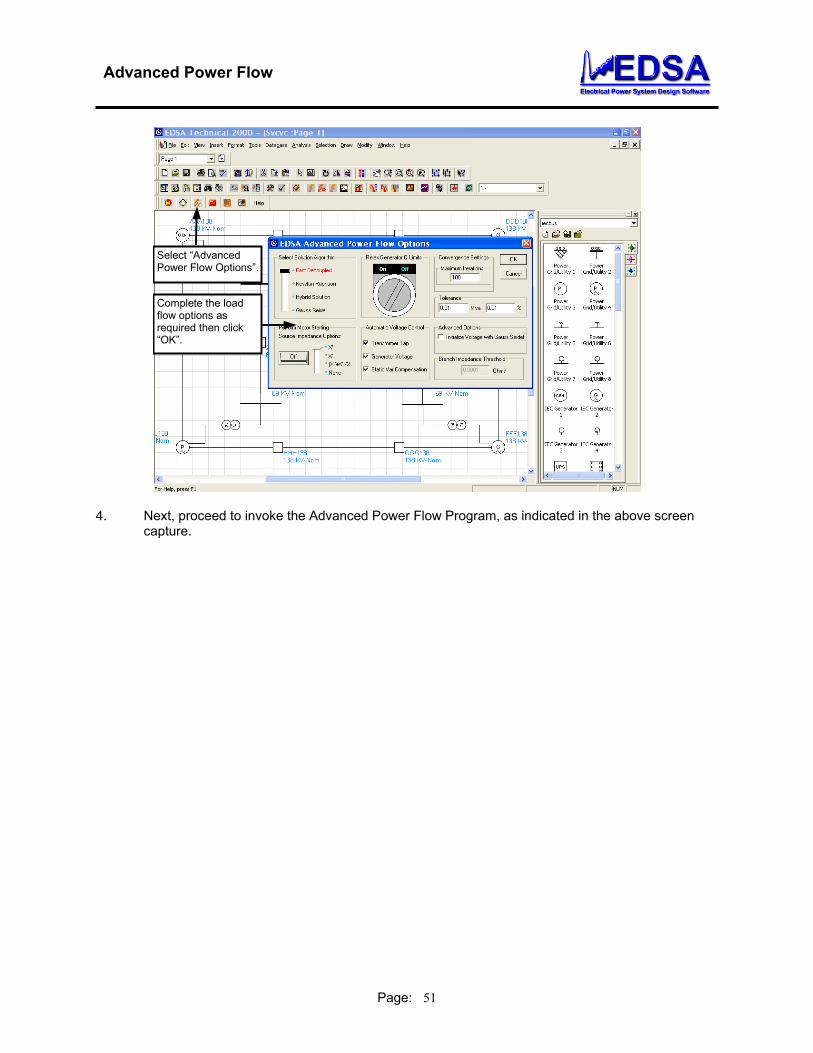
Select “Advanced Power Flow Options”.
Complete the load flow options as required then click “OK”.
4. Next, proceed to invoke the Advanced Power Flow Program, as indicated in the above screen capture.

Advanced Power Flow
Page: 52
Next, select “Analyze”.
Verify that the analysis has converged.
5. Run the analysis by following the instructions shown in the above screen capture.

Advanced Power Flow
Page: 53
Select “Report Manager”.
Next, select “View Full Power Flow Report Format 1”.
6. Once the calculations have been completed, proceed to view the output report as indicated in the above screen capture.

Advanced Power Flow
Page: 54
7. Once the calculations are completed, the results are shown in the Advanced Power Flow Output screen for “TD Load Flow Format 1”. With the aid of the tool bar menu, the user has the following options: Scroll up and down to read the results, Print the results, and Copy the results into the clipboard for importing purposes. From here, press DONE to return to the main menu.
8. “Save As” saves the output results in Microsoft Word format. However, when you open the
report, highlight the entire text, change the font to size 6, then save as a *.doc file.

Advanced Power Flow
Page: 55
19. Tutorial: Advanced Power Flow Based Motor Starting Analysis
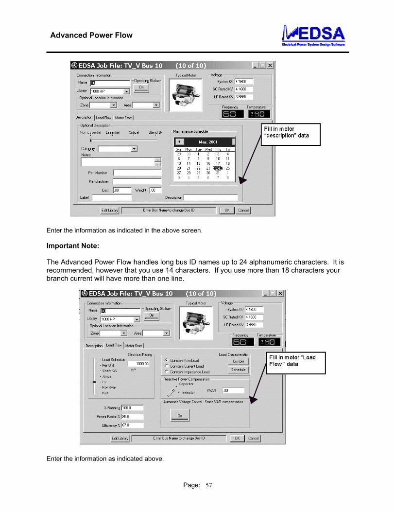
1. Invoke the EDSAT2K interface, and proceed to open the file called “tv_v” as indicated in the above screen capture.

Advanced Power Flow
Page: 56
Double-click on this motor to edit data and to be started.
2. Once the file is uploaded into EDSA Technical 2000 environment, it appears on the design space as shown above. As indicated in the screen capture, the motor 10 is going to be started. To define the characteristics of this motor, proceed as follows:
3. By double clicking the left mouse button, on the motor; you will then see the following screen
captures found on the next page.
Advanced Power Flow
Page: 57
Enter the information as indicated in the above screen.
Important Note: The Advanced Power Flow handles long bus ID names up to 24 alphanumeric characters. It is recommended, however that you use 14 characters. If you use more than 18 characters your branch current will have more than one line.
Enter the information as indicated above.

Advanced Power Flow
Page: 58
Finally, enter the Motor Start Data as indicated above.

Advanced Power Flow
Page: 59
Select “Advanced Power Flow Options”.
Complete the load flow options as required then click “OK”.
4. Next, proceed to invoke the Advanced Power Flow Program, as indicated above.
Next, select the “Motor Dynamic Information” icon.
5. Next, invoke the Motor Dynamic Data screen by following the steps in the above screen.
Advanced Power Flow
Page: 60
Step 1:Enter an appropriate description here.
Step 2: Enter the rated motor data.
Step 3:Select the “Rated Power” units.
Step 5: Enter the “Motor Moment of Inertia”. If the data are not known, select “Estimate”.
Step 6: Select “Solid State Voltage Control” Motor Starter.
Step 7: Select “Control Type.”
Step 8:Select “Time-Freq” characteristics.
Step 9: Select “Equivalent Circuit” tab.
Step 4: Enter the “Load Shaft Speed” and “Load Moment of Inertia”. Load speed can be different from motor speed if a load gear is presented.
6. Enter the information as indicated in the above screen capture.
Advanced Power Flow
Page: 61
Step 10: Enter the motor’s equivalent parameters here. If this data are not known, select “Calculate” to have the program estimate these values from the data entered.
Step 11: Enter the “Weighting Factors” (between 0.1 and 1) here. “1” for 100% degree of confidence/accuracy.
Step 12: Enter the motor “Locked Rotor” data here.
Step 13: Select “OK”.
7. Once you select the “Equivalent Circuit” tab, proceed to enter the data as indicated above.
Advanced Power Flow
Page: 62
8. Select “Torque Fitting” button to view the motor torque.
Advanced Power Flow
Page: 63
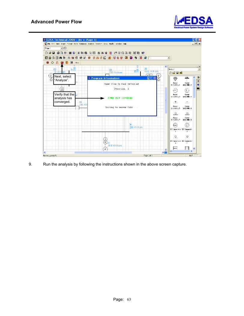
9. Run the analysis by following the instructions shown in the above screen capture.
Next, select “Analyze”.
Verify that the analysis has converged.

Advanced Power Flow
Page: 64
Select “Report Manager”.
To view the “Motor Starting Text Report”, click here.
To view the graphical output, click here.
10. Once the calculations have been completed, proceed to view the output report as indicated in the above screen capture. Notice that the “Motor Starting Reports” area is now active. The user may view the “Motor Starting Text Report” or “View Curves Graphically” as indicated in the above screen capture. You may also view “Export Results to Excel.”

Advanced Power Flow
Page: 65
11. The above screen capture shows the graphical output of the motor starting analysis. To exit,
press “Close”. Please test and try all the options made available for you in Select Charts, Grid Display, Background, Full Screen, etc.
A
B
C
D

Advanced Power Flow
Page: 66
12. The above screen capture shows the “Motor Starting Text Report”. With the aid of the tool bar menu, the user has the following options: Scroll up and down to read the results, Print the results, and Copy the results into the clipboard for importing purposes. From here, press DONE to return to the main menu.
13. “Save As” saves the output results in Microsoft Word format. However, when you open the
report, highlight the entire text, change the font to size 6, then save as a *.doc file.
Advanced Power Flow
Page: 67
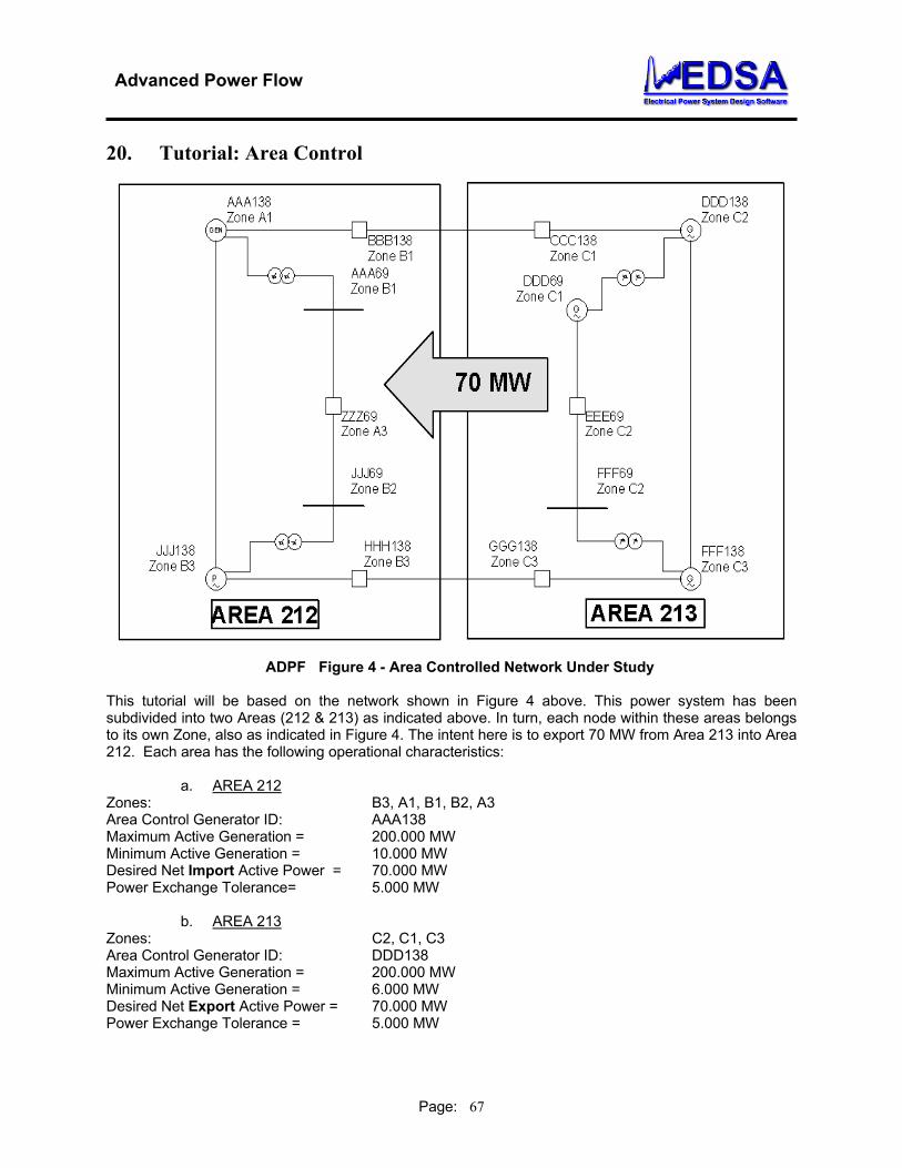
20. Tutorial: Area Control
ADPF Figure 4 - Area Controlled Network Under Study This tutorial will be based on the network shown in Figure 4 above. This power system has been subdivided into two Areas (212 & 213) as indicated above. In turn, each node within these areas belongs to its own Zone, also as indicated in Figure 4. The intent here is to export 70 MW from Area 213 into Area 212. Each area has the following operational characteristics:
a. AREA 212 Zones: B3, A1, B1, B2, A3 Area Control Generator ID: AAA138 Maximum Active Generation = 200.000 MW Minimum Active Generation = 10.000 MW Desired Net Import Active Power = 70.000 MW Power Exchange Tolerance= 5.000 MW
b. AREA 213 Zones: C2, C1, C3 Area Control Generator ID: DDD138 Maximum Active Generation = 200.000 MW Minimum Active Generation = 6.000 MW Desired Net Export Active Power = 70.000 MW Power Exchange Tolerance = 5.000 MW

Advanced Power Flow
Page: 68
1. Invoke the EDSAT2K, and proceed to load the pre-arranged file called “Areacont.axd”. The network should look as indicated in the above screen capture.

Advanced Power Flow
Page: 69
2. Enable the Area Interchange Control command, as indicated in the above screen capture.
Advanced Power Flow
Page: 70
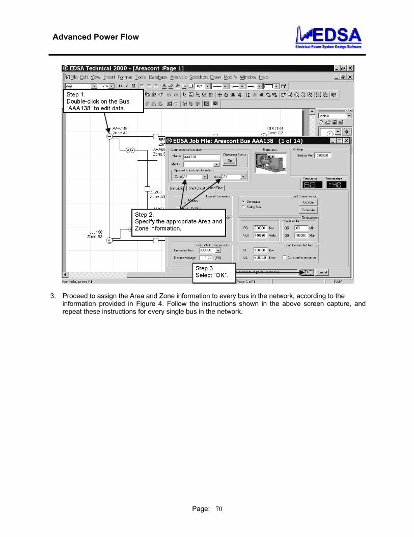
3. Proceed to assign the Area and Zone information to every bus in the network, according to the information provided in Figure 4. Follow the instructions shown in the above screen capture, and repeat these instructions for every single bus in the network.

Advanced Power Flow
Page: 71
Select “Advanced Power Flow Options”.
Complete the load flow options as required then click “OK”.
4. Proceed to invoke the Advanced Power Flow program, as indicated in the above screen capture.

Advanced Power Flow
Page: 72
Step 1: Select “Area Power Control Options.”
Step 2:Select Area “212”.
Step 3: Enter the required information here.
Step 5: Enter the required information here.
Step 4:Select Area “213”.
Step 6: Select “OK”.
5. Specify the Area Control parameters and run the Load Flow analysis, as indicated in the above screen capture.

Advanced Power Flow
Page: 73
Select “Report Manager”.
To view the “Area Interchange Report”, click here.
6. Once the calculations are completed, the results are shown in the Advanced Power Flow
Output screen for “Area Power Interchange”. With the aid of the tool bar menu, the user has the following options: Scroll up and down to read the results, Print the results, and Copy the results into the clipboard for importing purposes. From here, press DONE to return to the main menu.
Advanced Power Flow
Page: 74
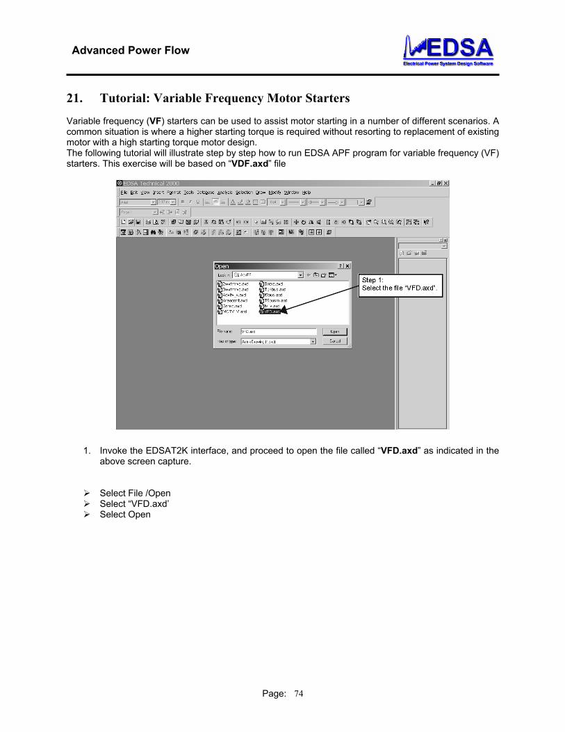
21. Tutorial: Variable Frequency Motor Starters Variable frequency (VF) starters can be used to assist motor starting in a number of different scenarios. A common situation is where a higher starting torque is required without resorting to replacement of existing motor with a high starting torque motor design. The following tutorial will illustrate step by step how to run EDSA APF program for variable frequency (VF) starters. This exercise will be based on “VDF.axd” file
1. Invoke the EDSAT2K interface, and proceed to open the file called “VFD.axd” as indicated in the above screen capture.
Select File /Open Select “VFD.axd’ Select Open
Advanced Power Flow
Page: 75
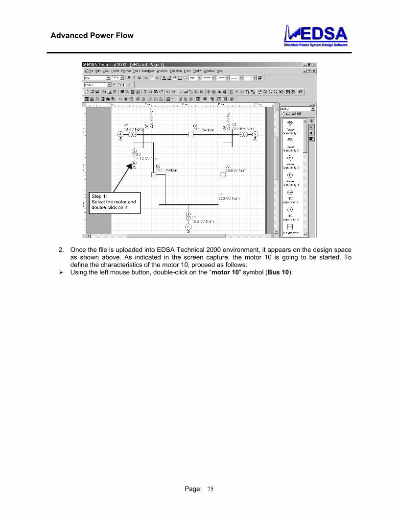
2. Once the file is uploaded into EDSA Technical 2000 environment, it appears on the design space as shown above. As indicated in the screen capture, the motor 10 is going to be started. To define the characteristics of the motor 10, proceed as follows:
Using the left mouse button, double-click on the “motor 10” symbol (Bus 10);

Advanced Power Flow
Page: 76
3. Follow the steps as indicated in the above screen capture.

Advanced Power Flow
Page: 77

Advanced Power Flow
Page: 78
4. Fill in the motor and motor starting data, as presented in the above screen capture.
Advanced Power Flow
Page: 79
Select “Advanced Power Flow Options”.
Complete the load flow options as required then click “OK”.
5. Select “AC Advanced with Motor Starting” program, as indicated in the above screen capture.
Next, select the “Motor Dynamic Information” icon.
6. Next, invoke the Motor Dynamic Data screen by following the steps in the above screen capture.

Advanced Power Flow
Page: 80
Step 1:Enter an appropriate description here.
Step 2: Enter the rated motor data.
Step 3:Select the “Rated Power” units.
Step 5: Enter the “Motor Moment of Inertia”. If the data are not known, select “Estimate”.
Step 6: Select “Solid State Voltage Control” Motor Starter.
Step 7:Select “Time-Freq” characteristics.
Step 8: Select “Equivalent Circuit” tab.
Step 4: Enter the “Load Shaft Speed” and “Load Moment of Inertia”. Load speed can be different from motor speed if a load gear is presented.
7. Fill in the required motor and motor staring data. Select the Motor Starter Method: Variable
Frequency Drive. In the above scenario, the applied motor frequency up to 3 seconds is 0.8 p.u. which is 48 Hz in a 60 Hz system. Then, the applied frequency will be 0.9 p.u. (54 Hz) for 2 seconds, and, finally the frequency return to nominal value at 5 seconds. The motor performance characteristics are shown on the next page:
Advanced Power Flow
Page: 81
8. If the Motor Parameters are not known, then the user selects “Calculate” button and the above
screen capture appears. Enter the “Weighting Factors” – 1 for 100% degree of confidence, 0 for 0% degree of confidence in introducing the motor data. The program automatically calculates the “Motor Parameters” presented at step 10 in the above screen capture.
Step 10: Enter the motor’s equivalent parameters here. If this data are not known, select “Calculate” to have the program estimate these values from the data entered.
Step 11: Enter the “Weighting Factors” (between 0.1 and 1) here. “1” for 100% degree of confidence/accuracy.
Step 12: Enter the motor “Locked Rotor” data here.
Step 13: Select “OK”.
Advanced Power Flow
Page: 82
9. Select “Torque Fitting” button to view the motor torque.
10. Run the analysis by following the instructions shown in the above screen capture.
Next, select “Analyze”.
Verify that the analysis has converged.

Advanced Power Flow
Page: 83
Select “Report Manager”.
To view the “Motor Starting Text Report”, click here.
To view the graphical output, click here.
11. Once the calculations have been completed, proceed to view the output report as indicated in the
above screen capture. Notice that the “Motor Starting Reports” area is now active. The user may view the “Motor Starting Text Report” or “View Curves Graphically” as indicated in the above screen capture. You may also view “Export Results to Excel.”

Advanced Power Flow
Page: 84
12. The above screen captures show the graphical output results of the motor starting analysis. To
exit, press “Close”. It is clear from the above chart that starting the motor with applied frequency less than nominal frequency provides higher starting torque. Of course, this also means that motor starting current will be higher but the design of VF is a trade off between the requirement of high starting torque and motor withstand capability of carrying higher current.
EDSA Advance Power Flow program can be successfully used to analyze the motor starting performances, and select the best starting method. Regarding VFD Motor Starting Method, it is clear from the above plots, that starting the motor with applied frequency less than nominal frequency provides higher starting torque. Of course, this also means that motor starting current will be higher, but the design of VF is a trade off between the requirement of high starting torque and motor withstand capability of carrying higher current.
Advanced Power Flow
Page: 85
22. Motor Decrement Export Function from Advanced Motor Starting to Protective Device Coordination
In this version, you can run EDSA Advanced Motor Starting , then export the time-current to *.csv/Excel, then import the motor time current from *.csv into EDSA Equipment folder. Once the data are in the folder, then you can go to Protective Device Coordination, bring up the Motor/Load and apply Fuse, Relay, Breaker and perform a complete coordination. See the steps below. First, you will need to open a job file. Go to File>Open Drawing File, then go to EDSAT2K\Samples\Transient and open Loadramp.axd.
Select
Now select .

Advanced Power Flow
Page: 86
Select
Then select
in EDSA Advanced Motor Starting. You will see the following screen on the next page.
Advanced Power Flow
Page: 87
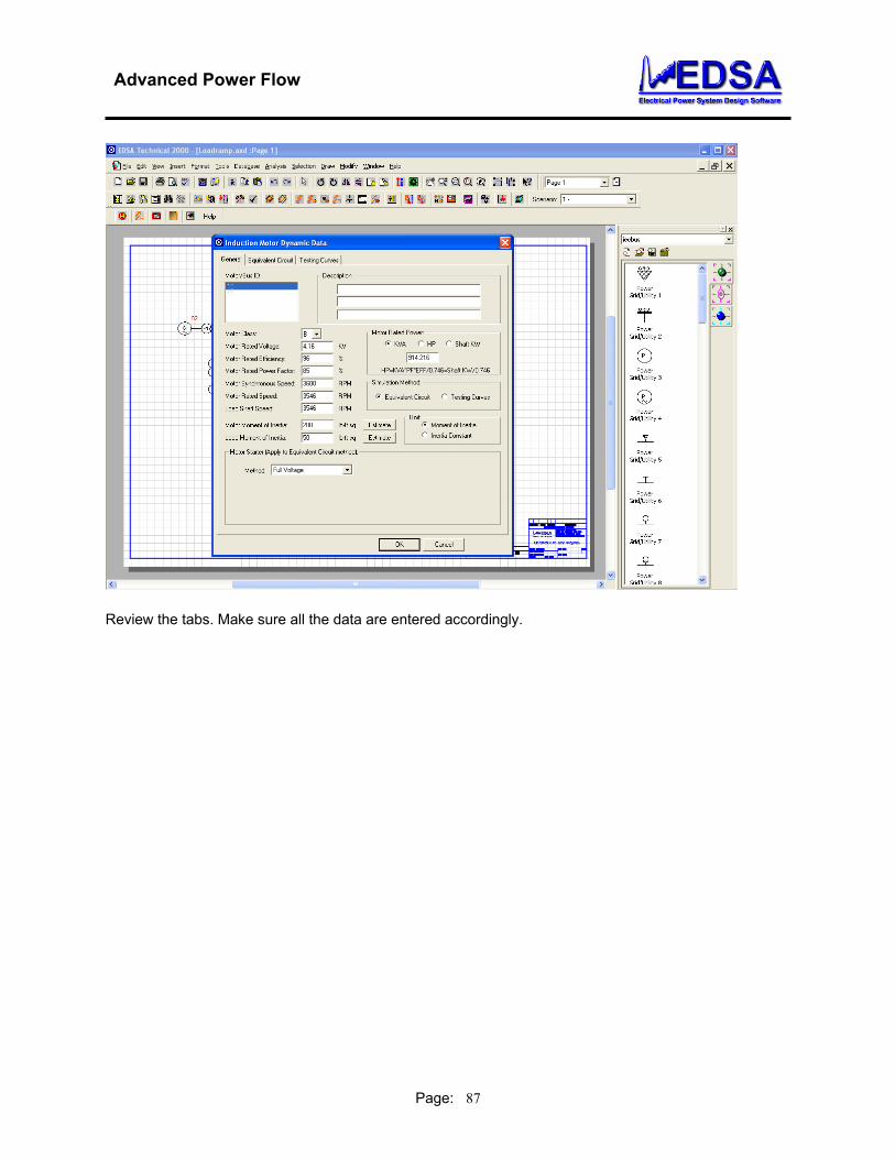
Review the tabs. Make sure all the data are entered accordingly.

Advanced Power Flow
Page: 88
1. Select
2. Select an Impedance.
3. Click “OK”.
Follow the steps as indicated and make sure to select “Power Source Impedance” option. Run the Advanced Motor Start by pressing “OK”.
Advanced Power Flow
Page: 89
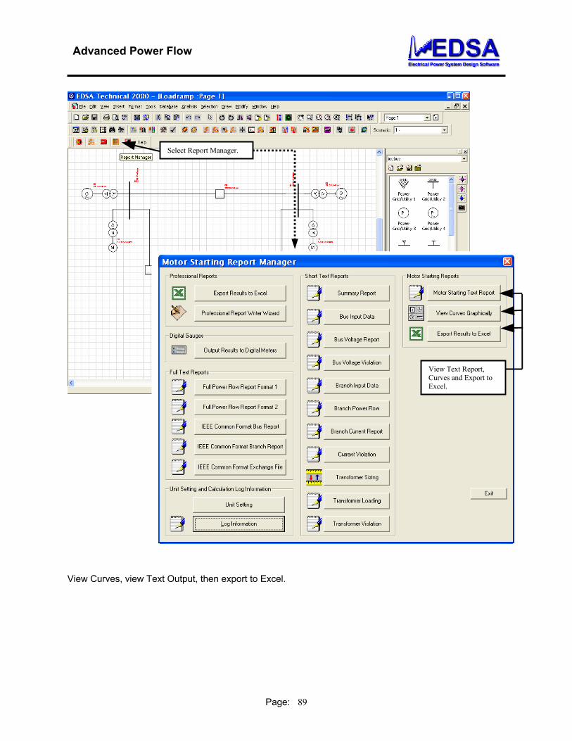
Select Report Manager.
View Text Report, Curves and Export to Excel.
View Curves, view Text Output, then export to Excel.
Advanced Power Flow
Page: 90
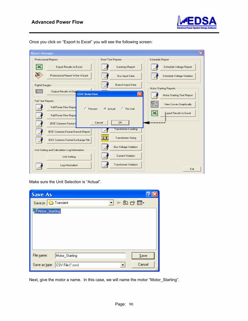
Once you click on “Export to Excel” you will see the following screen:
Make sure the Unit Selection is “Actual”.
Next, give the motor a name. In this case, we will name the motor “Motor_Starting”.
Advanced Power Flow
Page: 91
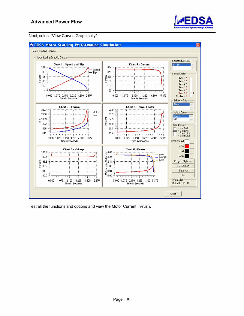
Next, select “View Curves Graphically”.
Test all the functions and options and view the Motor Current In-rush.
Advanced Power Flow
Page: 92
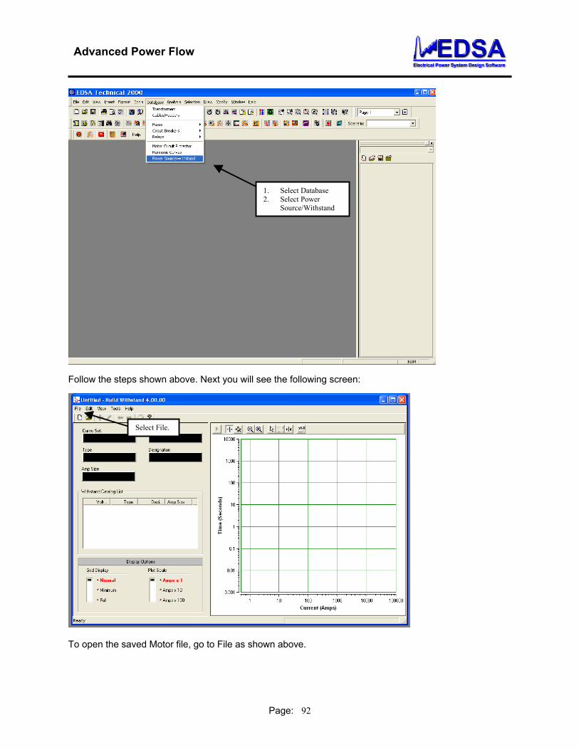
1. Select Database 2. Select Power
Source/Withstand
Follow the steps shown above. Next you will see the following screen:
Select File.
To open the saved Motor file, go to File as shown above.
Advanced Power Flow
Page: 93
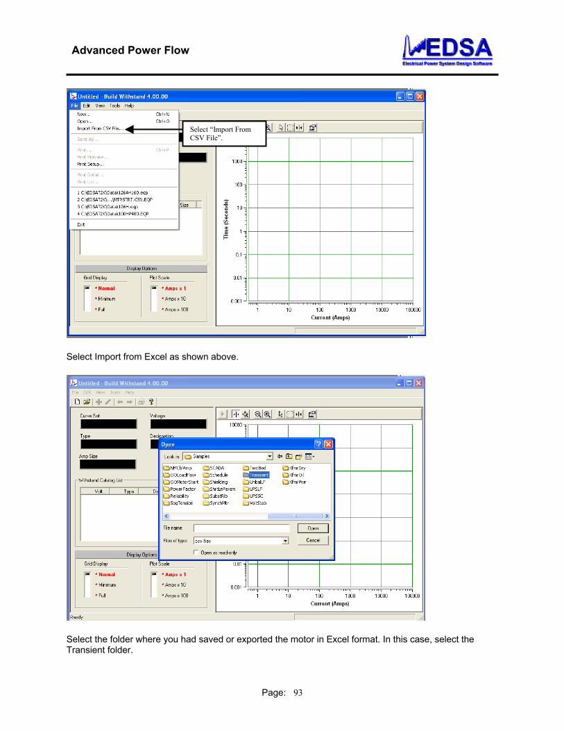
Select “Import From CSV File”.
Select Import from Excel as shown above.
Select the folder where you had saved or exported the motor in Excel format. In this case, select the Transient folder.

Advanced Power Flow
Page: 94
Select the Motor from Folder
Enter the data for both Description and Curves.
Edit and complete the motor data information, as shown above.

Advanced Power Flow
Page: 95
Next, review the Motor in-rush current and make sure it appears satisfactory.
Next, open the Standalone Protective Device Coordination by clicking the icon
.

Advanced Power Flow
Page: 96
You will see the following screen:
1.
2. 3.
1. Select Motor 2. Select Custom Motor 3. Go to the manufacturer and select the motor that was imported from Advanced Motor
Starting.

Advanced Power Flow
Page: 97
4. 5.
6.
4. Complete the data for Equipment Voltage and Design Load Amps. 5. Next complete the data for Short Circuit Amps and short circuit symbol. Be sure to use Auto
Select.

Advanced Power Flow
Page: 98
1.2.
Once the selection is complete and successful, you may save it and then proceed to select a device such as Relay, Fuse, Breaker, etc., for Coordination.

Advanced Power Flow
Page: 99
In this case, a GE Relay was selected. View the coordination above.
Advanced Power Flow
Page: 100
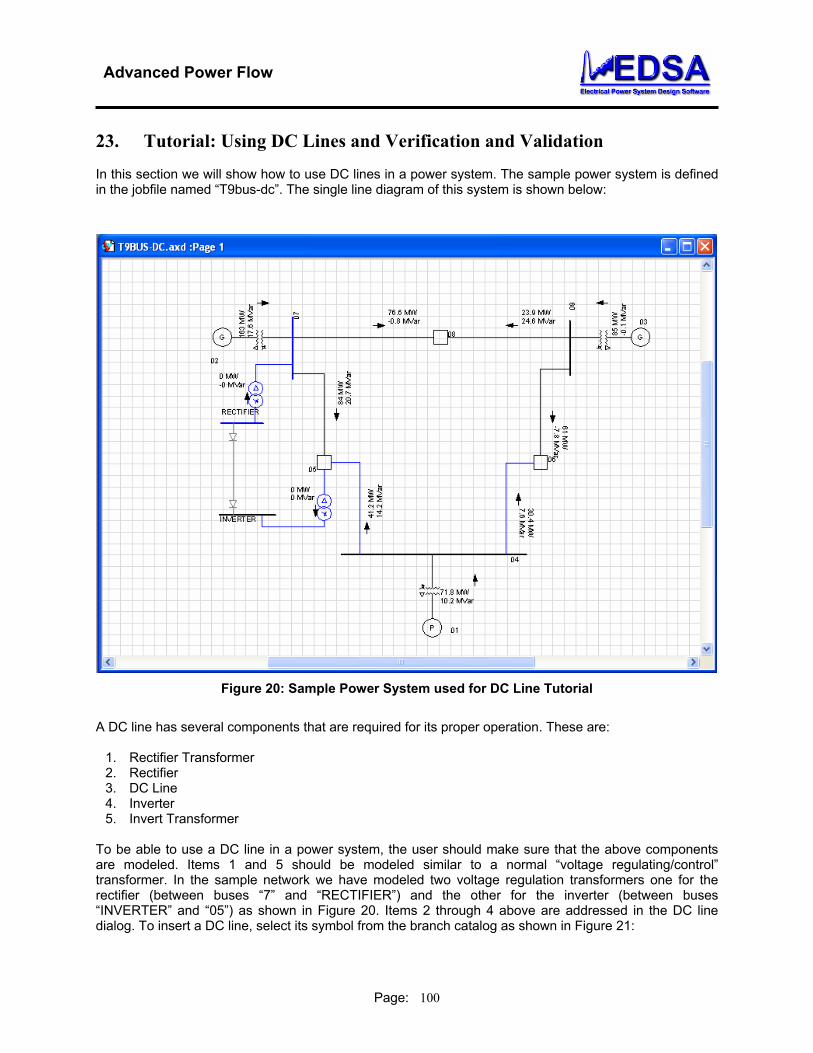
23. Tutorial: Using DC Lines and Verification and Validation In this section we will show how to use DC lines in a power system. The sample power system is defined in the jobfile named “T9bus-dc”. The single line diagram of this system is shown below:
Figure 20: Sample Power System used for DC Line Tutorial
A DC line has several components that are required for its proper operation. These are:
1. Rectifier Transformer 2. Rectifier 3. DC Line 4. Inverter 5. Invert Transformer
To be able to use a DC line in a power system, the user should make sure that the above components are modeled. Items 1 and 5 should be modeled similar to a normal “voltage regulating/control” transformer. In the sample network we have modeled two voltage regulation transformers one for the rectifier (between buses “7” and “RECTIFIER”) and the other for the inverter (between buses “INVERTER” and “05”) as shown in Figure 20. Items 2 through 4 above are addressed in the DC line dialog. To insert a DC line, select its symbol from the branch catalog as shown in Figure 21:

Advanced Power Flow
Page: 101
Figure 21: Selecting DC line Symbol
After selecting the DC line symbol drag it into single line diagram area and connect it to the buses “RECTIFIER” and “INVERTER” as seen in Figure 20.
Advanced Power Flow
Page: 102
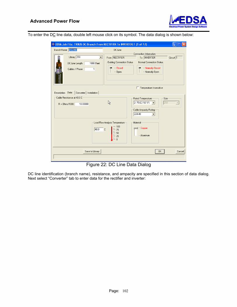
To enter the DC line data, double left mouse click on its symbol. The data dialog is shown below:
Figure 22: DC Line Data Dialog
DC line identification (branch name), resistance, and ampacity are specified in this section of data dialog. Next select “Converter” tab to enter data for the rectifier and inverter:

Advanced Power Flow
Page: 103
Figure 23: DC Line Data Dialog - Rectifier and Inverter
It is important to notice that the rectifier is always on the “From” side and inverter is on the “To” side as shown in the upper right part of the Figure 23. For both rectifier and inverter the user should specify number of bridges. For rectifier, the desired delay (also known as firing) angle as well as desired active power flow through DC line should be entered. For inverter, the minimum marginal angle (also known as extinction) angle as well as desired DC line voltage needs to be specified. The proper selection of the DC line voltage is crucial to DC line operation and solution convergence. To assist the user, the program can suggest an approximate value of the DC line voltage. Press “Estimate” button shown next to the field for “Desired DC Voltage”. For case at hand the program has calculated a value of 442.95 kV as shown in the above figure. For this example, let’s enter 450 kV as shown in Figure 24.
Advanced Power Flow
Page: 104
Figure 24: Rectifier and Inverter Data
After completing DC line data we solve the powerflow. The iteration report for the above sample network is shown below:
Mismatch Report Iteration No. kW Bus kVAR Bus 1 95169.2 INVERTER 77804.8 09 2 9410.5 05 12424.8 RECTIFIER 3 1129.3 05 2102.7 05 4 128.5 05 305.5 05 5 5299.7 07 30918.7 07 Ctrl Adjustments made for: V Ctrl 6 316.4 05 2281.4 RECTIFIER 7 67.8 05 207.6 RECTIFIER 8 5558.9 07 32905.5 07 Ctrl Adjustments made for: V Ctrl 9 202.5 INVERTER 2319.8 RECTIFIER 10 46.3 INVERTER 259.6 RECTIFIER 11 1900.5 07 31828.2 05 Ctrl Adjustments made for: V Ctrl

Advanced Power Flow
Page: 105
12 135.2 INVERTER 1437.8 INVERTER 13 28.5 INVERTER 335.6 INVERTER 14 1873.4 05 34005.4 05 Ctrl Adjustments made for: V Ctrl 15 75.6 05 1853.6 05 16 57.5 05 483.1 INVERTER 17 681.0 05 11754.3 05 Ctrl Adjustments made for: V Ctrl 18 45.8 05 736.0 05 19 24.5 05 189.6 INVERTER 20 6.1 05 38.0 INVERTER 21 1.4 05 8.6 INVERTER Ctrl Adjustments made for: DC 22 0.3 05 1.9 INVERTER Ctrl Adjustments made for: DC 23 0.7 INVERTER 0.5 INVERTER Ctrl Adjustments made for: DC *** Solution converged in 23 iterations
The above iteration report shows that the solution was achieved in 23 iterations. Also note that control adjustments were made for both voltage control transformers as well as DC line. The results of power flow for the sample system is shown Figure 25.

Advanced Power Flow
Page: 106
Figure 25: Power Flows Shown on the Single Line Diagram of the Sample Network
with DC Line The summary as well as branch reports are also shown below. It is important to note that in the branch report for DC line, the MVAR flow is not the reactive power flow on the DC line but it is the reactive power consumed in the rectifier and inverter. EDSA Advanced Power Flow Program V5.60.00 ========================================= Project No. : Page : 1 Project Name: Date : 11/11/2005 Title : Time : 03:13:50 pm Drawing No. : Company : Revision No.: Engineer : Jobfile Name: t9bus-dc Check by : Scenario : 1 - Date : A 9 bus system from Anderson "Power System Control and Stability" Page 38 Electrical One-Line 3-Phase to Single-Phase IEC project System Information ================== Base MVA = 100.000 (MVA) Frequency = 60 (HZ) Unit System = U.S. Standard MaxIterations = 1000 Error Tolerance = 0.001 (MVA), 0.000010 (PU), 0.0010 (%)
Advanced Power Flow
Page: 107
# of Buses entered = 11 # of Active Buses = 11 # of Swing Buses = 1 # of Generators = 2 # of Loads = 3 # of Shunts = 0 # of Lines entered = 12 # Total Branches/lines = 12 # of Transformers = 5 # of Reactors = 0 # of C.B. = 0 # of Open Switches = 0 Abbreviations ============= 2-W xfmr = 2-winding transformer None = None contributing 3-W xfmr = 3-winding transformer P_Load = Constant power load Autoxfmr = Autotransformer PhS xfmr = Phase-Shift Transformer DReactor = Duplex Reactor SeriesC = Series Capacitor F_Load = Functional load ShuntC = Shunt Capacitor FeederM = Feeder in Magnetic Conduit ShuntR = Shunt Reactor Gen = Generator Z_Load = Constant impedance load I_Load = Constant current load Ref °C = Reference Temperature Power Flow By Fast Decoupled CONVERGED Iteration: 23 Summary of Total Generation and Demand ====================================== P(MW) Q(MVAR) S(MVA) PF(%) Swing Bus(es): 70.908 25.357 75.305 94.16 Generators : 248.000 65.385 256.474 96.70 Shunt : 0.000 0.000 0.000 0.00 Static Load : 315.000 115.000 335.336 93.94 Motor Load : 0.000 0.000 0.000 0.00 Total Loss : 3.908 -24.259 ---------- ---------- Mismatch : 0.000 0.001 Generator & Capacitor/Inductor (SVC) Voltage Control ==================================================== Bus Name Controlled Bus DesiredV AchieveV GenV P Qmin Q Qmax (kV) (kV) (kV) (MW) (MVAR) (MVAR) (MVAR) ------------------------ ------------------------ -------- -------- -------- -------- -------- -------- -------- 02 02 18.450 18.450 18.450 163.00 -80.00 54.05 80.00 03 03 14.145 14.145 14.145 85.00 -40.00 11.33 40.00 Transformer Voltage Control & Line Voltage Regulator ==================================================== Branch Name C# Type Controlled Bus Name MinV CalcuV MaxV MinTap Tap MaxTap (kV) (kV) (kV) (PU) (PU) (PU) ------------------------ -- -------- ------------------------ -------- -------- -------- ------ ------ ------ INV-TRSFO 1 2-W xfmr INVERTER 327.750 353.622 362.250 0.900 0.910 1.100 REC-TRSFO 1 2-W xfmr RECTIFIER 327.750 352.069 362.250 0.900 0.952 1.100 DC Line Result ============== Branch Name Type Library CodeName From kV To kV Current Firing Extinction (kA) Ang (Deg.) Ang (Deg.) ------------------------ -------- ---------------- -------- -------- -------- ---------- ---------- DCLINE DC Line 250 451.911 450.000 0.191 15.72 17.60 Branch Power Flow Values ======================== Branch Name C# Type Library CodeName From -> To Flow To -> From Flow Losses (MW) (MVAR) (MW) (MVAR) (MW) (MVAR) ------------------------ -- -------- ---------------- -------- -------- -------- -------- -------- --------

Advanced Power Flow
Page: 108
04 ->05 1 Feeder 250 19.92 33.62 -19.70 -48.19 0.22 -14.57 04 ->06 1 Feeder 250 -50.53 -1.30 50.98 -11.53 0.46 -12.83 05 ->07 1 Feeder 250 -19.94 -38.48 20.30 11.33 0.36 -27.15 06 ->09 1 Feeder 250 40.16 -4.21 -39.47 -28.70 0.68 -32.91 07 ->08 1 Feeder 250 55.71 -7.69 -55.44 -4.82 0.27 -12.51 08 ->09 1 Feeder 250 -44.56 -30.18 44.84 11.44 0.29 -18.74 DCLINE 1 DC Line 250 86.36 27.35 -86.00 31.09 0.37 58.45 01 ->04 1 2-W xfmr 1000-3-D 70.91 25.36 -70.91 -22.09 0.00 3.27 02 ->07 1 2-W xfmr 1000-3-D 163.00 54.05 -163.00 -36.51 0.00 17.54 03 ->09 1 2-W xfmr 1000-3-D 85.00 11.33 -85.00 -7.23 0.00 4.10 INV-TRSFO 1 2-W xfmr 1000-3-D -85.36 36.67 86.00 -31.09 0.64 5.57 REC-TRSFO 1 2-W xfmr 1000-3-D 87.00 32.87 -86.36 -27.35 0.63 5.52
Verification and Validation of DC Line Model Since there are no published examples of power flow solution including DC line, the following approach is adopted here. The power flow solution of the above system without DC line will be compared with the solution with DC line and the reasonability of the result will be argued. Let’s start the discussion by first examining the power flows reaching bus 05 for the case with DC line: From Figure 25: Flow from bus 07 to 05 19.9 MW Flow from bus 04 to 05 19.9 MW Flow from INVERTER to 05 85.4 MW Total Flow reaching bus 05 125.2 MW Now, let’s examine the power flow reaching bus 05 for the case without DC line (DC Line is open): From Figure 20: Flow from bus 07 to 05 84.0 MW Flow from bus 04 to 05 41.2MW Total Flow reaching bus 05 125.2 MW The difference of total power reaching bus 05 in two cases is 125.2-125.2 / 125.2 *100 = 0 %. Based on the above evidence, it is concluded that EDSA advanced power flow program accurately models DC lines. DC Line Sample Network 2 A second example for the DC line is provided below. This example (jobfile named “T14bus-dc”) is similar to the sample power system used in the jobfile named “T14bus”. We have added rectifier and inverter transformer as shown below:

Advanced Power Flow
Page: 109
Figure 26: Example of a Power System using DC Line, “T14bus-dc”
The data for the rectifier and inverter for this system is shown below:

Advanced Power Flow
Page: 110
Figure 27: DC Line Data for the Sample Network using DC Line
The solution is shown in Figure 26 and the text result report is shown below: EDSA Advanced Power Flow Program V5.60.00 ========================================= Project No. : Page : 1 Project Name: Date : 11/11/2005 Title : Time : 03:46:23 pm Drawing No. : Company : Revision No.: Engineer : Jobfile Name: t14bus-dc Check by : Scenario : 1 - Date : A 14-bus network shown in Fig.E.3 in Paul M. Anderson's Faulted Power Systems System Information ================== Base MVA = 100.000 (MVA) Frequency = 60 (HZ) Unit System = U.S. Standard MaxIterations = 100 Error Tolerance = 0.010 (MVA), 0.000100 (PU), 0.0100 (%) # of Buses entered = 16 # of Active Buses = 16 # of Swing Buses = 1 # of Generators = 4 # of Loads = 9 # of Shunts = 4 # of Lines entered = 19 # Total Branches/lines = 19 # of Transformers = 6 # of Reactors = 0 # of C.B. = 0 # of Open Switches = 0
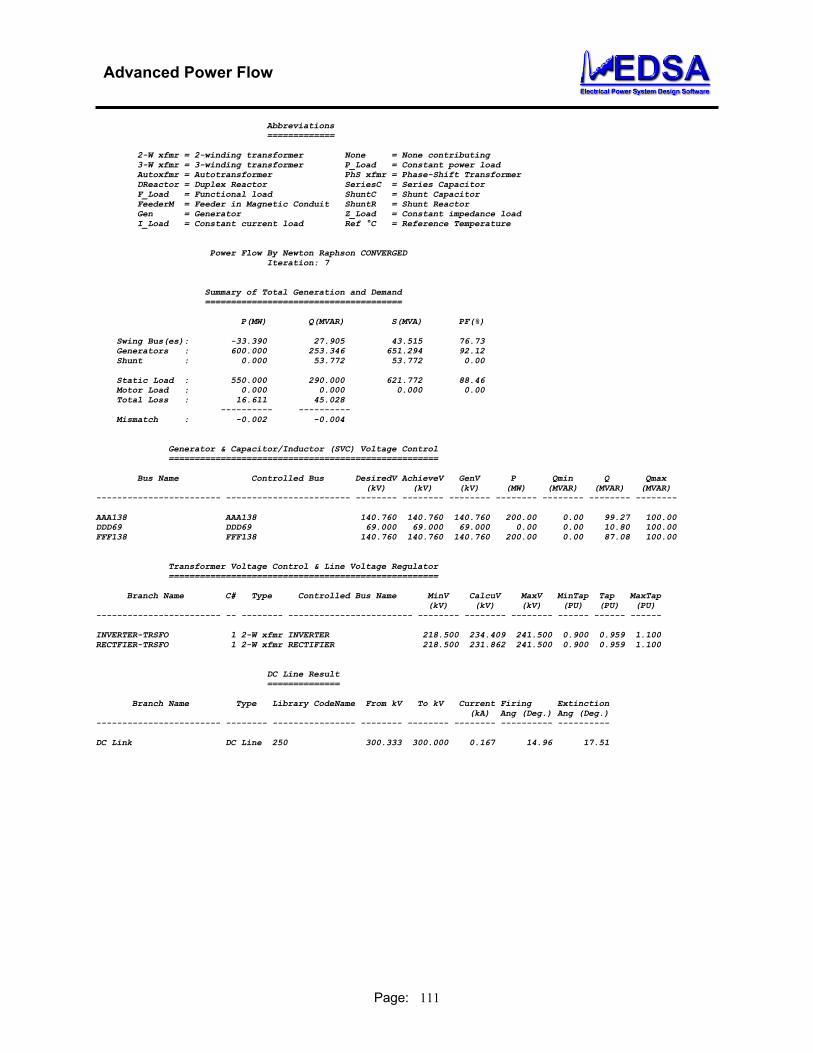
Advanced Power Flow
Page: 111
Abbreviations ============= 2-W xfmr = 2-winding transformer None = None contributing 3-W xfmr = 3-winding transformer P_Load = Constant power load Autoxfmr = Autotransformer PhS xfmr = Phase-Shift Transformer DReactor = Duplex Reactor SeriesC = Series Capacitor F_Load = Functional load ShuntC = Shunt Capacitor FeederM = Feeder in Magnetic Conduit ShuntR = Shunt Reactor Gen = Generator Z_Load = Constant impedance load I_Load = Constant current load Ref °C = Reference Temperature Power Flow By Newton Raphson CONVERGED Iteration: 7 Summary of Total Generation and Demand ====================================== P(MW) Q(MVAR) S(MVA) PF(%) Swing Bus(es): -33.390 27.905 43.515 76.73 Generators : 600.000 253.346 651.294 92.12 Shunt : 0.000 53.772 53.772 0.00 Static Load : 550.000 290.000 621.772 88.46 Motor Load : 0.000 0.000 0.000 0.00 Total Loss : 16.611 45.028 ---------- ---------- Mismatch : -0.002 -0.004 Generator & Capacitor/Inductor (SVC) Voltage Control ==================================================== Bus Name Controlled Bus DesiredV AchieveV GenV P Qmin Q Qmax (kV) (kV) (kV) (MW) (MVAR) (MVAR) (MVAR) ------------------------ ------------------------ -------- -------- -------- -------- -------- -------- -------- AAA138 AAA138 140.760 140.760 140.760 200.00 0.00 99.27 100.00 DDD69 DDD69 69.000 69.000 69.000 0.00 0.00 10.80 100.00 FFF138 FFF138 140.760 140.760 140.760 200.00 0.00 87.08 100.00 Transformer Voltage Control & Line Voltage Regulator ==================================================== Branch Name C# Type Controlled Bus Name MinV CalcuV MaxV MinTap Tap MaxTap (kV) (kV) (kV) (PU) (PU) (PU) ------------------------ -- -------- ------------------------ -------- -------- -------- ------ ------ ------ INVERTER-TRSFO 1 2-W xfmr INVERTER 218.500 234.409 241.500 0.900 0.959 1.100 RECTFIER-TRSFO 1 2-W xfmr RECTIFIER 218.500 231.862 241.500 0.900 0.959 1.100 DC Line Result ============== Branch Name Type Library CodeName From kV To kV Current Firing Extinction (kA) Ang (Deg.) Ang (Deg.) ------------------------ -------- ---------------- -------- -------- -------- ---------- ---------- DC Link DC Line 250 300.333 300.000 0.167 14.96 17.51


