56
Advanced Decision Analysis: Markov Models

Advanced Decision Analysis: Markov Models

Reasons to understand Markov models
• It’s the standard in academia • Very powerful/flexible tool
– simple decision trees • relatively inflexible
– limited time frame – hard to model recurring risks
– Markov models: • allow you to model anything (well, almost anything)
Challenges of Markov models
• More difficult conceptually than simple decision tree models
• Trickier math – rates vs. probabilities

Overview • Introduction to Markov models
– Problems with simple decision trees – Markov models
• general structure • how they run • rates & probabilities • how they keep score (expected value)


Should patients with Bjork-Shiley valves undergo prophylactic replacement?
Risks of Outlet Strut Fracture (and its consequences)
vs. Risks with reoperation

Clinical Scenario
• 65 year man with prosthetic valve in 1986 – otherwise healthy
• predicted operative risk 3%
– 29mm, 70° Björk-Shiley valve • strut fracture risk 10.5% at 8 years • 63% case-fatality

Decision Analysis
1. structure competing strategies and clinical outcomes in a decision model
2. estimate probabilities for clinical outcomes 3. assign values for clinical outcomes (utility) 4. analysis • calculate expected values of strategies • assess stability of results (sensitivity analysis)
Four Basic Steps

1. Structure model (simple tree) die
survive/well strut fracture
no fracture/well
watchful waiting
die
survive prophylactic reop
choose

2. Assign probabilities die
0.63 survive/well
strut fracture 0.105
no fracture/well 0.895
watchful waiting
die 0.03
survive 0.97
prophylactic reop
choose 0.37
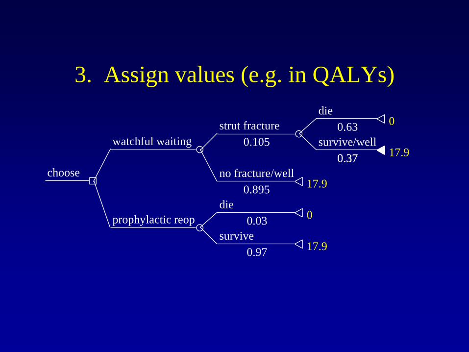
3. Assign values (e.g. in QALYs) die
0.63 0
survive/well 0.37 17.9
strut fracture 0.105
no fracture/well 0.895 17.9
watchful waiting
die 0.03 0
survive 0.97 17.9
prophylactic reop
choose 0.37

4(a). Baseline analysis die
0.63 0
survive
0.37 17.9
strut fract
0.105
no fracture
0.895 17.9
watch wait
die
0.03 0
survive
0.97 17.9
proph reop
choose 0.37
U*P
0
0.7
16.0
0
17.4
16.7 QALYS
17.4 QALYS
EV

4(b). Sensitivity analysis
16.0
16.4
16.8
17.2
17.6
18.0
Expected Value (QALYs)
10 8 6 4 2 0
Operative Mortality Risk (%)
Prophylactic Reoperation
Watchful Waiting
Bas
elin
e
Thr
esho
ld

Limitations of simple decision trees
• Don’t account for timing of events – Roll the dice once, at time zero
• Problems with parameter estimates (time) – probabilities, dealing with competing risks over
time – values applied to future outcomes may be
underestimated (all bad events considered to be happening immediately)

Problems with simple trees die
0.63 0
survive/well 0.37 17.9
strut fracture 0.105
no fracture/well 0.895 17.9
watchful waiting
die 0.03 0
survive 0.97 17.9
prophylactic reop
choose 0.37
EV 17.4
EV 16.7
What if the person lived 20 good years before dying from strut fracture? EV=0???
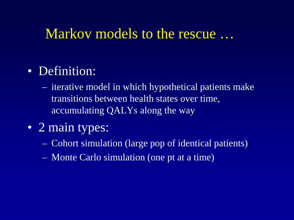
Markov models to the rescue …
• Definition: – iterative model in which hypothetical patients make
transitions between health states over time, accumulating QALYs along the way
• 2 main types: – Cohort simulation (large pop of identical patients) – Monte Carlo simulation (one pt at a time)
Decision analysis with Markov models
• Same four basic steps as simple trees – structuring the model – probabilities – assigning values to outcomes – baseline and sensitivity analysis
• But a little more complex …

Model structures viewed left to right
• Simple trees – specify alternatives
(decision node) – chance events (chance
nodes) – final health states
(terminal nodes)
• Markov models – specify alternatives
(decision node) – parse to health states
(intermediate and final) – chance events move
hypothetical patients between health states

Specifying alternatives
watchful waiting
prophylactic reop
choose

Health states well
well, postop
dead
watchful waiting
well, postop
dead
prophylactic reop
choose
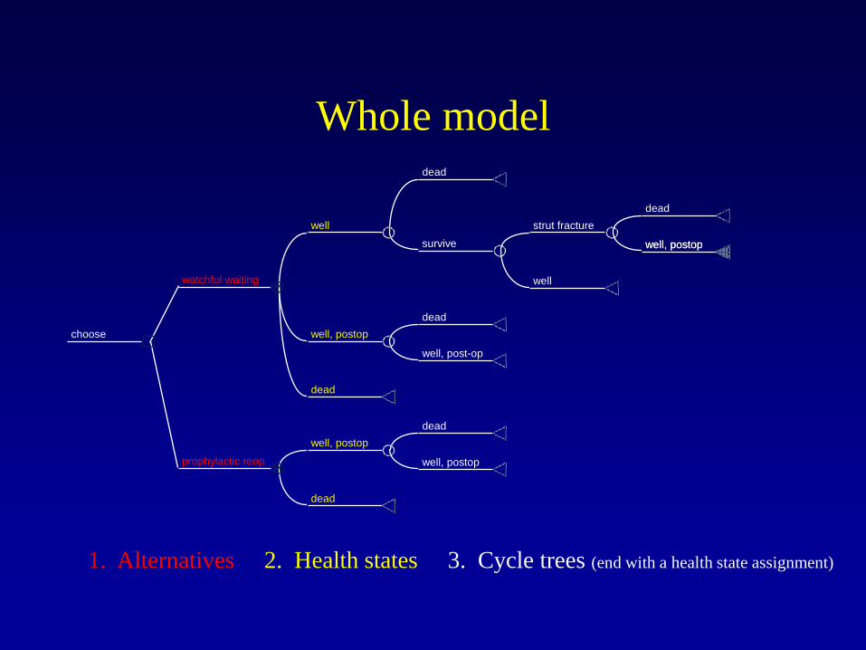
Whole model dead
dead
well, postop
strut fracture
well
survive
well
dead
well, post-op
well, postop
dead
watchful waiting
dead
well, postop
well, postop
dead
prophylactic reop
choose
well, postop
1. Alternatives 2. Health states 3. Cycle trees (end with a health state assignment)

How the model “runs”
• Markov cohort simulation – hypothetically large cohort – start in distribution of health states at time zero – some members make transitions between health
states with each cycle (Cycle = “stage” in TreeAge)
– keep cycling until everyone (or nearly everyone) absorbed into the state “dead”

Folding back: Time zero well
well, postop
dead
watchful waiting
well, postop
dead
prophylactic reop
choose
cycle length = 1 year
1000 pts
0 pts
0 pts
970 pts
30 pts
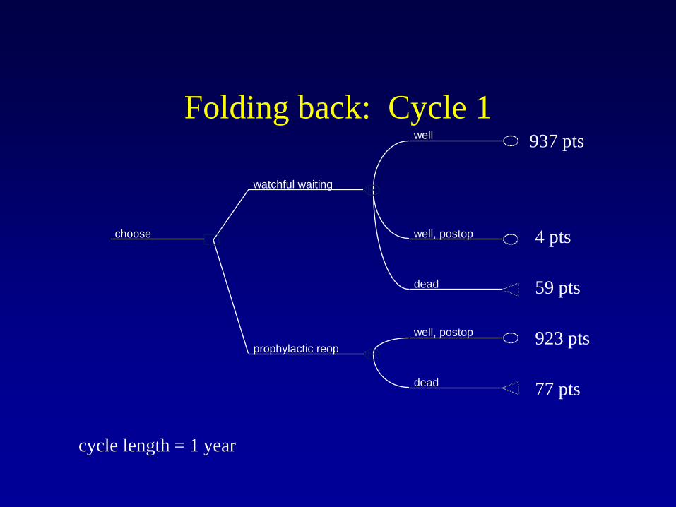
Folding back: Cycle 1 well
well, postop
dead
watchful waiting
well, postop
dead
prophylactic reop
choose
cycle length = 1 year
937 pts
4 pts
59 pts
923 pts
77 pts

Folding back: Cycle 10 well
well, postop
dead
watchful waiting
well, postop
dead
prophylactic reop
choose
cycle length = 1 year
540 pts
12pts
448pts
556 pts
444 pts
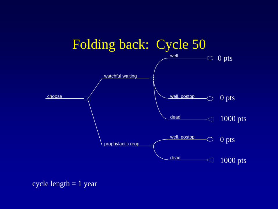
Folding back: Cycle 50 well
well, postop
dead
watchful waiting
well, postop
dead
prophylactic reop
choose
cycle length = 1 year
0 pts
0 pts
1000 pts
0 pts
1000 pts

Decision analysis with Markov models
• Four components – structuring the model (and how it runs) – probabilities – assigning values to outcomes – analysis

Probabilities
Events with short time horizons (e.g., op risk)
Events that occur over time (e.g., valve-failure)
Constant Changing
Simple trees Markov models

Events with short time horizons (easy) dead
dead
well, postop
strut fracture
well
survive
well
dead
well, post-op
well, postop
dead
watchful waiting
dead
well, postop
well, postop
dead
prophylactic reop
choose
well, postop
1. Alternatives 2. Health states 3. Cycle trees *
*

Events occurring over time (harder) dead
dead
well, postop
strut fracture
well
survive
well
dead
well, post-op
well, postop
dead
watchful waiting
dead
well, postop
well, postop
dead
prophylactic reop
choose
well, postop
1. Alternatives 2. Health states 3. Cycle trees
* *
*
*
Probabilities of events occurring during each cycle of the model (aka transition probabilities)
What you need:
Published studies don’t give you cycle-specific probabilities
Problem:
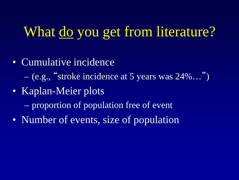
What do you get from literature?
• Cumulative incidence – (e.g., “stroke incidence at 5 years was 24%…”)
• Kaplan-Meier plots – proportion of population free of event
• Number of events, size of population

Deriving transition probabilities
Data from source studies
Annual rates
Cycle-specific probabilities
Step 1
Step 2

Step 1. Deriving rates
Source Data x-year probability (% pts with event at x years) survival / event-free curve (% pts [f] without event) # events
Rate Formula ln (1 - p) t ln (f) t # events/pt-yrs follow-up
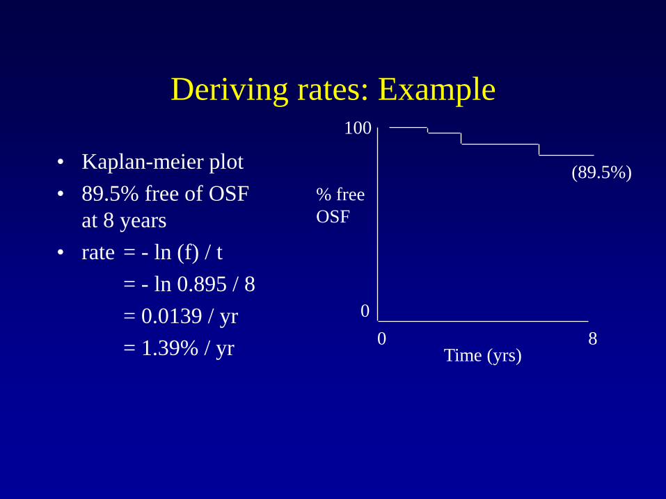
Deriving rates: Example
• Kaplan-meier plot • 89.5% free of OSF
at 8 years • rate = - ln (f) / t = - ln 0.895 / 8 = 0.0139 / yr = 1.39% / yr Time (yrs)
0 8
% free OSF
0
100
(89.5%)

Deriving transition probabilities
Data from source studies
Rates
Cycle-specific probabilities
Step 1
Step 2

Step 2. Converting rates to transition probabilities
• Transition probability (p) = 1 – e^(-r * t) – r = rate, t = cycle length
• Example: – Strut Fx rate = 0.0139; 3 month cycle length p = 1 – e^(-0.0139 * 0.25) = 0.00347
• TreeAge function: “RateToProb”


Decision analysis with Markov models
• Four components – structuring the model (and how it runs) – probabilities – assigning values to outcomes – analysis

Assigning values (rewards)
• Simple trees: – one value assigned each terminal node
• Markov: – assigned at each health state – can be credited multiple times (with each cycle
of the model)

Assigning values to health states (“rewards”)
• Measures of expected value – Costs ($), years of life, QALYs

Accumulating rewards: Cycle 0 to 1 well
well, postop
dead
watchful waiting
well, postop
dead
prophylactic reop
choose
Incremental reward = cycle length = 1 year
1000 pts
0 pts
0 pts
970 pts
30 pts
Cycle 1000 Cum 1000 Cycle 970 Cum 970

Accumulating rewards: Cycle 1 to 2 well
well, postop
dead
watchful waiting
well, postop
dead
prophylactic reop
choose
Incremental reward = cycle length = 1 year
937 pts
4 pts
59 pts
923 pts
77 pts
Cycle 941 Cum 1941 Cycle 923 Cum 1893

Accumulating reward: Cycle 10 to 11 well
well, postop
dead
watchful waiting
well, postop
dead
prophylactic reop
choose
Incremental reward = cycle length = 1 year
540 pts
12pts
448pts
556 pts
444 pts
Cycle 552 Cum 7822 Cycle 556 Cum 7810

Accumulating reward: Cycle 50 well
well, postop
dead
watchful waiting
well, postop
dead
prophylactic reop
choose
Incremental reward = cycle length = 1 year
0 pts
0 pts
1000 pts
0 pts
1000 pts
Cycle 0 Cum 17145 Cycle 0 Cum 17411

Baseline analysis
Strategy Cumulative reward
Expected Value
Watchful Waiting
17,145
Prophylactic Reoperation
17,411

Baseline analysis
Strategy Cumulative reward
Expected Value
Watchful Waiting
17,145 17.1 years/person
Prophylactic Reoperation
17,411 17.4 years/person

How do you incorporate utilities?

Accumulating rewards: Cycle 0 to 1 well
well, postop
dead
watchful waiting
well, postop
dead
prophylactic reop
choose
Incremental reward = 0.5 * 1 year
1000 pts
0 pts
0 pts
970 pts
30 pts
Cycle 500 Cum 500 Cycle 485 Cum 485

?

Building a Decision Model Your patient is a 65 year old white male with a large abdominal aortic aneurysm. Although asymptomatic, the aneurysm has grown substantially over the last year, from 4.6cm to 6.0cm. You have decided that the aneurysm needs repair. However, the patient also has severe angina and a positive stress test, and cardiac catheterization reveals good ventricular function, but severe coronary disease that is not amenable to PTCA or stenting. Question: Should this patient undergo AAA repair only, AAA repair followed by CABG, or CABG prior to AAA repair?

Basic Steps
1. Structure a decision model 2. Enter probabilities, life expectancy and
utility values 3. Perform a baseline analysis 4. Perform sensitivity analysis


