Advanced Internet Technologies

Advanced Internet Technologies, SS 2004 3.1

Advanced Internet TechnologiesChapter 3

Performance Modeling

Dr.-Ing. Falko Dressler

Chair for Computer Networks & InternetWilhelm-Schickard-Institute for Computer Science

University of Tübingen

http://net.informatik.uni-tuebingen.de/[email protected]


Chapter 3Performance Modeling

Queuing AnalysisIntroductionQueuing Models

Self-Similar Traffic


Queuing Analysis – Introduction

GoalsPrediction of network/system behaviorPerformance modeling and estimation

BenefitsReal-world tests are expensive and often infeasibleAnalytic models based on queuing theory often provide the neededanswers

Queue

Server


How Queues Behave – A Simple Example

Consider a system with the following capabilitiesCapacity of input and output: 1000 packets/sProcessing time for an average request: 1msUnlimited queue sizeNon-uniform arrival rate

Three experimentsArrival rate of 500 requests/s (50% server capacity)Arrival rate of 950 requests/s (95% server capacity)Arrival rate of 990 requests/s (99% server capacity)


Queue Behavior with Normalized Arrival Rate of 0.5

ResultsAvg buffer size: 43Peak: >600








Performance Evaluation

1. Do an after-the-fact analysis based on actual values2. Make a simple projection by scaling up from existing experience to the expected future

environment3. Develop an analytic model based on queuing theory4. Program and run a simulation model


Queuing Models – Single-Server Queue

Theoretical maximum input rate that can be handled by the system(at utilization ρ=1):

smax

1T

=λ


Single-Server Queue – Model Characteristics (Assumptions)

Item populationItems arrive from an infinite source populationThus, the arrival rate is not altered as items enter the system(If the population is finite, then the population available for arrival is reduced by the number of items currently in the system; this would typically reduce the arrival rate proportionally)

Queue sizeThe queue size is infiniteThus, the queue can grow without bound(With a finite queue, items can be lost from the system; that is, if the queue is full and additional items arrive, some items must be discarded)

Dispatching disciplineWhen the server becomes free, and if there is more than one item waiting, a decision must be made as to which item to dispatch nextExamples: FIFO, FCFS, LIFO, ...


Example of a Queuing Process


Notations


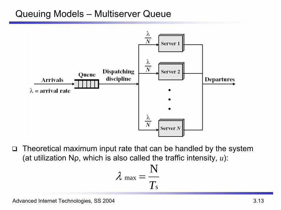
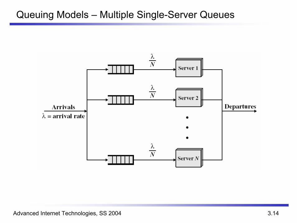
Queuing Models – Multiserver Queue

Theoretical maximum input rate that can be handled by the system(at utilization Nρ, which is also called the traffic intensity, u):

smax

NT

=λ


Queuing Models – Multiple Single-Server Queues


Queuing Analysis - Basics

Input informationArrival rate: λService time: Ts

Number of servers: N

Average values (w, Tw, r, Tr)Standard deviation (σw, σTw, σr, σTr)

Output informationItems waiting: wWaiting time: Tw

Items queued: rResidence time: Tr


Queuing Analysis – Basics II

Distribution of the interarrival timesTypically, we assume that the interarrival time is exponential,which is equivalent to saying that the number of arrivals in a period t obeys the Poisson distribution,which is equivalent to saying that the arrivals occur randomly and independent of one another.

Kendall’s notationX/Y/N

X refers to the distribution of the interarrival timesY refers to the distribution of service timesN refers to the number of servers

DistributionsG ... General distribution of interarrival timesGI ... General distribution of interarrival times, interarrival times are independedM ... Poisson distributionD ... Deterministic distribution

ExampleM/M/1 refers to a single-server queuing model with Poisson arrivals


Single-Server Queues


Single-Server Queues II

Mean number of items in system for single-server queue


Single-Server Queues III

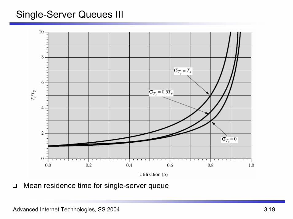
Mean residence time for single-server queue


Single-Server Queues IV

σTs/Ts is also known as the coefficient of variation and gives a normalized measure of variability

The meaning of σTs/Ts

Zero: constant service time, e.g. if all transmitted packets are of the same lengthRatio less then 1: ratio better than the exponential case, the M/M/1 model would give answers on the safe sideRatio close to 1: common occurrence, corresponds to exponential service timeRatio greater than 1: the M/G/1 model is required


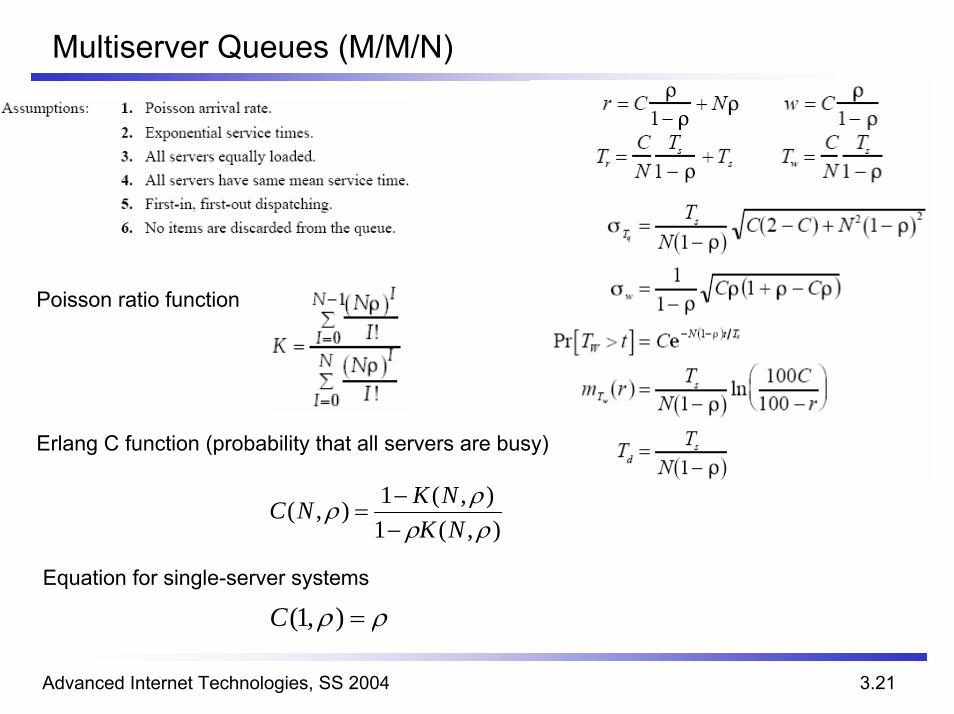
Multiserver Queues (M/M/N)

),(1),(1),(ρρρρ

NKNKNC

−−

=

Poisson ratio function

Erlang C function (probability that all servers are busy)

Equation for single-server systems

ρρ =),1(C


An Example – Single-Server Model

Engineers use PCs plus a single graphic workstation. On a typical 8-hour day, 10 engineers will use the workstation and spend an average of 30 minutes at a session.

Average time an engineer spendswaiting for the workstation

Average rate of engineers

Average number of engineers waiting

minutes 501

=−

=ρ

ρ sw

TT

minuteengineers/ 021.060*8

10==λ

engineers 0416.1== wTw λ


An Example – Single-Server Model II

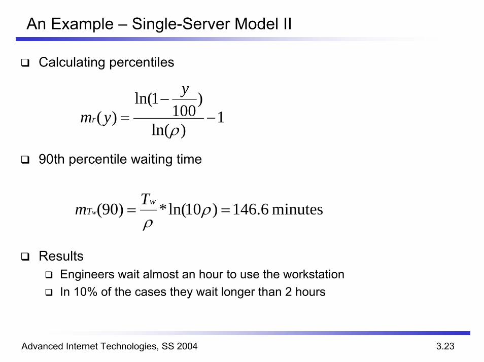
Calculating percentiles

90th percentile waiting time

ResultsEngineers wait almost an hour to use the workstationIn 10% of the cases they wait longer than 2 hours

1)ln(

)100

1ln()( −

−=

ρ

y

ymr

minutes 6.146)10ln(*)90( == ρρ

wT

Tm w


An Example – Multiserver Model

Probability that both servers are busy

Average time an engineer spendswaiting for a workstation

90th percentile waiting time

Average number of engineers waiting

engineers 07.0== wTw λ

minutes 247.3)1(=

−=

ρNCTT s

w

minutes 67.8)10ln(*)1(2

)90( =−

= CTm sTw

ρ

0.1488)C(2,0.3125)C(2, ==ρ


An Example – Single-Server vs. Multiserver Model


Network of Queues

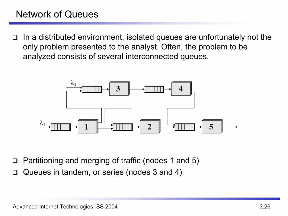
In a distributed environment, isolated queues are unfortunately not the only problem presented to the analyst. Often, the problem to be analyzed consists of several interconnected queues.

Partitioning and merging of traffic (nodes 1 and 5)Queues in tandem, or series (nodes 3 and 4)


Network of Queues – Partitioning and Merging

PartitioningIf the incoming distribution is Poisson, then the two departing traffic flows also have Poisson distributions, with mean rates Pλ and (1-P)λ.

MergingIf two Poisson streams with mean rates λ1 and λ2 are merged, the resulting stream is Poisson with a mean rate of λ1 + λ2.


Network of Queues – Queues in Tandem

Assume that the input to the first queue is Poisson. Then, if the service time of each queue is exponential and the queues are of infinitecapacity, the output of each queue is a Poisson stream statistically identical to the input. Thus, the queues are independent and may be analyzed one at a time. Therefore, the mean total delay for the tandem system is equal to the sum of the mean delay at each stage.


Jackson’s Theorem

AssumptionsThe queuing network consists of m nodes, each of which provides an independent exponential service.Items arriving from outside the system to any one of the nodes arrive with a Poisson rate.Once served at a node, an item goes (immediately) to one of the other nodes with a fixed probability, or out of the system.

Jackson’s TheoremJackson’s theorem states that in such a network of queues, each node is an independent queuing system, with Poisson input determined by the principles of partitioning, merging, and tandem queuing. Thus, each node may be analyzed separately from the others using the M/M/1 or M/M/N model, and the results may be combined by ordinary statistical methods.


Self-Similar Traffic

Queuing analysis depends on the Poisson nature of the data trafficIt has shown that for some environments the traffic pattern is self-similar rather than Poisson

Self-similarity is a concept related to two othersFractalsChaos theory

OutlinePhenomenon of self-similarityPerformance implicationsStorage Model with Self-Similar


Self-Similarity

Statement by Manfred-Schroeder:

The unifying concept underlying fractals, chaos, and power laws is self-similarity. Self-similarity, or invariance against changes in scale or size, is an attribute of many laws in nature and innumerable phenomena in the world around us. Self-similarity is, in fact, one of the decisive symmetries that shape our universe and our effort to comprehend it.


Self-Similarity – An Example

Network monitoring, analysis of the interarrival time of single framesMinimum transmission time for one frame: 4ms

Recorded arrivals (ms):0 8 24 32 72 80 96 104 216 224 240 248 288 296 312 320648 656 672 680 720 728 744 752 864 872 888 896 936 944 960 968

Clustering all samples with gaps smaller than 20ms:0 72 216 288 648 720 864 936

Clustering all samples with gaps smaller than 40ms:0 216 648 864


Self-Similarity – An Example II

Repeating patterns: arrival, short gap, arrival, long gap, arrival, short gap, arrival)

0

200

400

600

800

1000

1200

1 3 5 7 9 11 13 15 17 19 21 23 25 27 29 31

Gap

s be

twee

n si

ngle

fram

es /

clus

ters

[ms] Reihe1

Reihe2Reihe3


Self-Similarity – An Example III

Repeating patterns: arrival, short gap, arrival, long gap, arrival, short gap, arrival)


Cantor Set

Famous construct appearing in virtually every book on chaos, fractals, and nonlinear dynamicsConstruction rules:

Begin with the closed interval [0,1], represented by a line segmentRemove the open middle third of a lineFor each succeeding step, remove the middle third of the lines left by the preceding step

Cantor set:S0 = [0, 1]S1 = [0, 1/3] U [2/3, 1]S3 = [0, 1/9] U [2/9, 1/3] U [2/3, 7/9] U [8/9, 1]


Cantor Set II

Properties of Cantor sets seen in all self-similar phenomenaIt has a structure at arbitrarily small scales. If we magnify part of the set repeatedly, we continue to see a complex pattern of points separated by gaps of various sizes. The process seems unending. In contrast, when we look at a smooth, continuous curve under repeated magnification, it becomes more and more featureless.The structure repeat. A self-similar structure contains smaller replicas of itself at all scales. For example, at every step, the left (and right) portion of the Cantor set is an exact replica of the full set in the preceding step.

These properties do not hold indefinitely for real phenomena. At some point under magnification, the structure and the self-similarity break down. But over a large range of scales, many phenomena exhibit self-similarity.


Stochastical Self-Similarity

So far, we examined exact self-similarity:A pattern is reproduced exactly at different scales

Data traffic is a stochastic process, therefore we talk about statistical self-similarity.For a stochastic process, we say that the statistics of the process do not change with the change in the time scale. The average behavior of the process in the short-term is the same as it is in the long term.

ExamplesData trafficEarthquakesOcean wavesFluctuations in the stock market


Self-Similar Stochastic Process


Examples of Self-Similar Data Traffic

Ethernet TrafficW. Leland, M. Taqqu, W. Willinger: On the Self-Similar Nature of Ethernet Traffic.”Proceedings of the SIGCOMM ’93, September 1993.

World-Wide Web TrafficM. Crovella, A. Bestavros: “Self-Similarity in World-Wide Web Traffic: Evidence and Possible Causes.” Proceedings of the ACL Sigmetrics Conference on Measurement and Modeling of Computer Systems, May 1996.

Signaling System Number 7 (SS7) TrafficD. Duffy, A. McIntosh, M. Rosenstein, W. Willinger: “Statistical Analysis of CCSN/SS7 Traffic from Working CCS Subnetworks.” IEEE Journal on Selected Areas in Communication, April 1994.

TCP, FTP, and TELNET TrafficV. Paxson, S. Floyd: “Wide Area Traffic: The Failure of Poisson Modeling.”IEEE/ACM Transactions on Networking, June 1995.

Variable-Bit-Rate (VBR) VideoM. Garnett, W. Willinger: “Analysis, Modeling, and Generation of Self-Similar VBR Video Traffic.” Proceedings of the SIGCOMM ’94, August 1994.


Performance Implications – Ethernet Traffic


Storage Model with Self-Similar Input

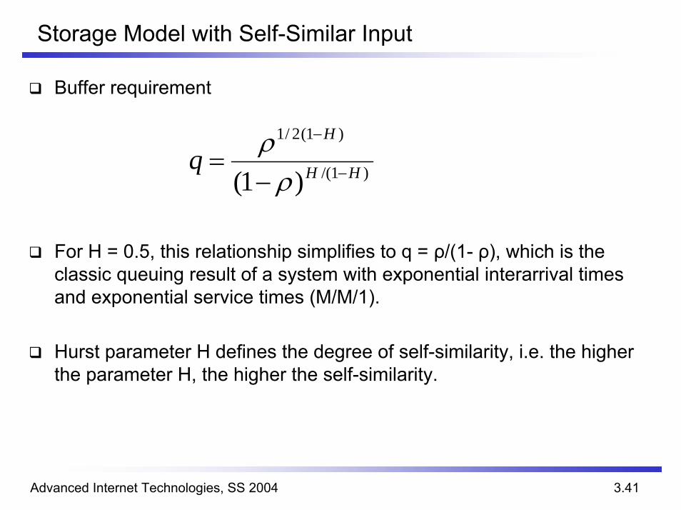
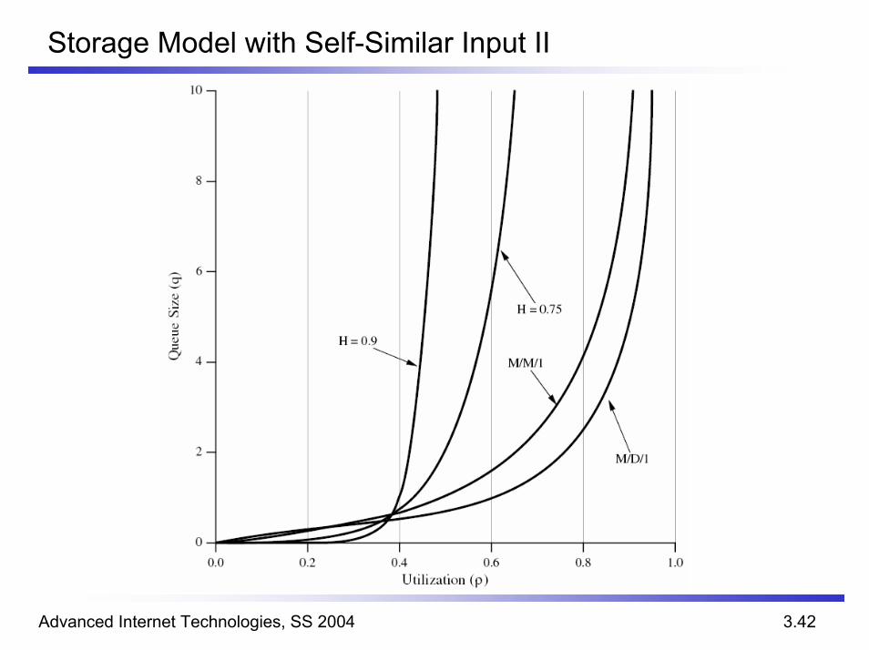
Buffer requirement

For H = 0.5, this relationship simplifies to q = ρ/(1- ρ), which is the classic queuing result of a system with exponential interarrival times and exponential service times (M/M/1).

Hurst parameter H defines the degree of self-similarity, i.e. the higher the parameter H, the higher the self-similarity.

)1/(

)1(2/1

)1( HH

H

q −

−

−=

ρρ


Storage Model with Self-Similar Input II

Date post:	04-Feb-2022
Category:	Documents
Upload:	others
View:	4 times
Download:	0 times

Advanced Internet Technologies

Documents