1936-23 Advanced School on Synchrotron and Free Electron Laser Sources and their Multidisciplinary Applications Aldo Craievich 7 - 25 April 2008 University de Sao Paulo Brazil Small angle x-ray scattering (Basic Aspects)
Transcript
1936-23
Advanced School on Synchrotron and Free Electron Laser Sourcesand their Multidisciplinary Applications
Aldo Craievich
7 - 25 April 2008
University de Sao PauloBrazil
Small angle x-ray scattering(Basic Aspects)
Small-Angle Xndashray Scattering by Nanostructured Materials
Aldo Craievich Institute of Physics University of Satildeo Paulo craievichifuspbr
ldquoWhen scientists have learned how to control the arrangement of matter at very small scale they will see materials take an enormously richer variety of propertiesrdquo R Feymman (1959)
1Basic introduction
The description of the characteristics of the small-angle X-ray scattering by materials will be introduced trough the simple example of an optical diffraction experiment in which a visible light beam passes through a small hole of a few microns on an opaque or semi-opaque mask This experiment can be performed using a simple laser source as those commonly utilized as a pointer in class-rooms (wavelength λasymp065 microm) What we may expect to see in a flat screen located at a distance D much larger than λ (say D=5m) from the mask (Fig1a) Classical physical optics tells us that a isotropic diffuse spot should be observed centered in the intersection of the transmitted beam with the screen Since the spot has a circular symmetry the scattering intensity is a function only of the scattering angle ε or of the distance on the screen defined by x (xasympεD) The scattering intensity function I1(ε) exhibits a maximum at ε=0 and its half maximum intensity width ∆ε increases for decreasing hole sizes These effects are qualitatively illustrated in Fig 1b 1c and 1d which display a series of three schematic profiles of the light scattering intensity produced by holes of different sizes
Fig 1 (a) Setup of an experiment of small angle light scattering (b) (c) and (d) are schematic
intensity curves corresponding to circular holes of different sizes
Incident beam (λ=065microm) Transmitted beam
Mask Screen Scattered beam
x
D
ε
(a)
I(ε)
I(ε) I(ε)
x
R1asymp1microm R2asymp5 microm R3asymp20 microm
x x
(b) (c) (d)
2
In practice the scattering intensity produced by a single hole is very weak and therefore the masks that are used in actual experiments contain many holes How the fact of having a number of holes instead of only one may affect the profile of the scattered intensity In order to answer this question the relevant features of the scattering intensity produced by different types of masks containing a number of identical circular holes arranged in different ways will be described
(i) Randomly located holes (2D ideal gas structure Fig 2a) The randomness condition can only be approximately fulfilled if the holes are very far apart from
each other A (very) dilute set of N randomly located holes produces a scattering intensity simply given by I(ε)= NI1(ε) This result implies that the hole positions are completely uncorrelated and consequently the total scattering intensity is the sum of the individual intensities i e no interference between wavelets generated by different holes occurs
(ii)Holes with short range spatial correlation (2D liquid-like structure Fig 2b) The scattered wavelet produced by each hole interferes with the others and thus the simple equation
I(ε)= NI1(ε) is not longer obeyed The interference effects due to the spatial correlation in hole positions are accounted for by the ldquostructure functionrdquo S(ε) so that I(ε)=NI1(ε)S(ε) The structure function for a set of holes with short-range order is different from 1 at small scattering angles and tends to 1 at high angles
(iii)Periodically arranged holes (2D crystal-like structure Fig 2c) In this case for particular values of the angle ε (ε=εn) the wavelets corresponding to the scattering
produced by all holes are in phase Thus the total scattering amplitude is A(εn)=NA1(εn) where A1 refers to the amplitude produced by each hole and A(εneεn)=0 The total intensity 2)()( εε AI = is then given by I(ε=εn)=N2I1(εn) and I(εneεn)=0 The structure function S(q) is composed of narrow peaks with non zero values (S(q)=N) for well-defined angles εasympεn which only depend on the geometry of the arrangement of holes This is analogous to the effects described by the well-known Bragg law corresponding to the X-ray diffraction by 3D crystals
Fig 2 Schematic masks and corresponding light scattering intensity for (a) a gas-like (dilute) set
of holes (b) a liquid-like (concentrated) set of holes with short range spatial order and (c) a crystal-like concentrated set of holes with long range spatial order
All previous considerations also apply to the case where instead of circular holes on a plane we
have spheres located in the three dimensional space
I(ε)
ε
(a) (b) (c)
I(ε)
ε
I(ε)
ε
B C
3
Elastic scattering of X-rays by nanostructured materials is a phenomenon similar to the described scattering of visible light by a mask with micrometric holes A 3D analogous of the mask may be a material containing nano-pores or an arrangement of nano-clusters The individual pores or clusters play the same role in X-ray scattering experiments as the microscopic holes in the mask The small-angle scattering is produced by electron density heterogeneities at nanometric level such as in the mentioned example the clusters or pores As it will be seen the small-angle X-ray scattering technique provides relevant information about the shape size size distribution and spatial correlation of heterogeneities in electron density
The properties of nanostructured materials are often very different from those of the same materials in bulk state They depend not only on the structure at atomic scale but also and often strongly on the structure at nanometric scale For example relatively small variations in the shape andor size of metal or semiconductor nanocrystals embedded in a glass matrix induce dramatic changes in the optical properties of these nanocomposites This example illustrates why the characterization of materials at a nanometric scale is a relevant issue for materials scientists Furthermore it will be demonstrated along this chapter that small-angle scattering technique actually is a very useful technique for structural characterizations at a nanometric scale
2 Small-angle X-ray scattering by nanostructured materials with an
arbitrary structure The basic process of the scattering of X-ray by materials is the photon-electron interaction As it
will be seen the X-ray scattering intensity produced by any material varies with the scattering angle and the characteristics of this function directly depend on the electron density function ( )rρ The electron density function contains all the information that is practically needed in order to fully describe the material structure
X-ray scattering by materials is named as ldquosmall-angle X-ray scatteringrdquo (or SAXS) when the measurements are confined to angles smaller than ~10 degrees These measurements provide relevant information if the average radius of the clusters andor inter-cluster distances are about 5-500 times the wavelength used in the experiment (typically λ=15 Aring) On the contrary if the objects are very large as compared to the X-ray wavelength (with sizes above say 1microm) the scattering intensity is concentrated within a extremely small angle domain close to the direct X-ray beam that is hidden by the narrow direct beam stopper placed close to the detector On the other hand the X-ray scattering at small-angles does not contain any information about the oscillations in electron density associated to the atomic nature of the structure This information can only be found at wide scattering angles These comments imply that the window of sizes that are probed by the small-angle X-ray scattering technique ranges from about 10 Aring up to 1000 Aring
The experiments of small-angle X-ray scattering are usually performed in transmission mode Thus for a wavelength much larger than 15 Aring photons would be strongly absorbed by the sample On the other hand if a much smaller wavelength is used the scattering would concentrate at too small angles making practical analyses difficult Therefore most of the SAXS experiments reported in the literature are performed using X-ray wavelengths ranging from 07 to 17 Aring
21 Scattering of x-rays by an electron The elastic scattering produced by an isolated electron was derived by Thompson The amplitude of
the wave scattered by each electron has a well-defined phase relation with the amplitude of the incident wave thus making interference effects possible In the particular case of a non-polarized X-ray beam such as those produced by a classical X-ray tube the scattering power of one electron per solid detection angle Ie is a function of the angle between the incident and the scattered beam 2θ
4
)2
2cos1()2(2
20
θθ += ee rII (1)
where I0 is the intensity of the incident beam (powercm2) and re is the classical radius of the electron
2262 10907 cmreminus= For small scattering angles 12cos2 asympθ so as the scattering intensity per electron
is simply given by 2
0)2( ee rII =θ (2) If a crystal monochromator is inserted in the beam path the X-ray beam becomes partially
polarized and Eq (1) does not longer hold but at small angles Eq (2) remains still valid as a good approximation
In addition to the coherent or elastic X-ray scattering the electrons also produce inelastic Compton scattering Compton scattering being incoherent (i e no phase relationship exists between incident and scattered waves) the scattered waves do not interfere and thus the scattering intensity is not modulated by structure correlation effects On the other hand since the intensity of Compton scattering within the small-angle range is weak its contribution can in practice be neglected
As the scattering intensity per electron Ie will later appear in all the equations defining the scattering intensity produced by materials it will be omitted for brevity
22 General equations The scattering amplitude and intensity related to the elastic interaction between a narrow
monochromatic X-ray beam ndash with a wavelength λ - and an arbitrary material are functions of the scattering vector q which is usually defined as the difference between the wave-vectors Q and 0Q - both with modulus equal to λπ2 - having the directions of the scattered and incident beam respectively (Fig 3) Since Q and 0Q are proportional to the linear momentum of the scattered and
incident photons ( Qhp = h being the Plank constant) respectively the difference 0QQq minus= is proportional to the photon momentum transfer qhp =∆ associated to the photon scattering process As illustrated in Fig 3 the modulus of q is 4π sin θλ θ being half the scattering angle
Fig 3 X-ray beam paths from the source to the detector both elements located far away from the
sample The segment BCAB + is the optical path difference from which the phase shift is determined
A B
Source
Detector 0
ε=2θ
r
Q
0Q
q
0Q
Q
C
5
The basic theory of X-ray scattering by a 3D material whose structure is defined by an electron density function )(rρ will be presented The electron density function may represent the high resolution structure ndash including its successive more or less high peaks corresponding to single atoms of different types - or only the low resolution structure ndash exclusively accounting for the nanometric features of the material A low resolution electron density function describes for example the shape and size of nano-precipitates embedded in a solid or liquid matrix but not their detailed crystallographic structure
The amplitude of the X-ray wavelet produced by the scattering of the electrons located inside a particular volume element dv is
ϕρ ∆= i
e edvrAqdA )()( (3)
where Ae is the amplitude of the wavelet scattered by one electron and dvr )(ρ is the number of electrons in the volume element dv dvrAe )(ρ is the modulus of the amplitude of the scattered wavelet and ϕ∆ie is a phase factor that accounts for the phase difference ϕ∆ between the wavelets associated to the scattering by electrons in a volume element located at 0=r and in another arbitrary volume element dv The amplitude eA will be set equal to 1 in the following equations for brevity
The optical path difference ∆s associated with two wavelets corresponding to the X-ray scattering by electrons inside a volume element at 0=r and another at r (Fig 3) is
)ˆˆ( 0 rQrQBCABs minusminus=+=∆ (4)
where 0Q and Q are unit vectors in the directions defined by 0Q and Q respectively Thus the phase shift defined as λπϕ s∆=∆ 2 becomes
rqrQQrQQ )()ˆˆ(2 00 minus=minusminus=
minusminus=∆
λπϕ (5)
Substituting ϕ∆ in Eq (3) and integrating over the whole volume V the total scattering amplitude (setting eA =1) is given by
dverqA rqi
V
)()( minusint= ρ (6)
This is the amplitude of the scattered waves under the assumptions of the kinematical theory of X-
ray scattering disregarding multiple scattering and absorption effects [1] Eq (6) indicates that )(qA simply is the Fourier transform of the electron density )(rρ The amplitude )(qA is defined in the reciprocal or Fourier space ( q space) and is a complex function i e its value is specified by the real and imaginary parts or alternatively but the modulus and phase
Inversely the electron density )(rρ can mathematically be obtained by a Fourier transformation of the amplitude function )(qA
( ) q
rqi dveqAr 3 )(
21)( int=π
ρ (7)
6
Taking into account the mathematical properties of the Fourier transformation we know that the electron density )(rρ defining the high-resolution material structure (i e the atomic configuration) can only be determined if the complex function )(qA (modulus and phase) is known over a large volume in q space On the other hand if the amplitude )(qA is known only within a rather small volume in q space close to q =0 Eq (7) yields the low-resolution features of the structure
Nevertheless a fundamental difficulty arises in the analysis of the results of scattering experiments because the X-ray detectors count photons ie what is experimentally determined is the scattering intensity )(qI and not the complex amplitude )(qA Since 2 )()()()( qAqAqAqI == the square root of the measured )(qI function provides only the modulus of the scattering amplitude
[ ] 21)()( qIqA = (8) Thus Eq (7) cannot be directly applied to derive neither the electron density function )(rρ and
consequently nor the material structure This is the known phase problem that crystallographers and materials scientists always face when they try to determine the detailed material structure from the results of X-ray scattering experiments
A procedure that can be applied to determine simple low resolution structures circumventing the phase problem is to begin with a proposed structure model providing an initial guessed electron density function )(rρ The scattering amplitude is determined using Eqs (6) and then the trial intensity
2)()( qAqI = is compared to the experimental intensity The use of ad-hoc iterative computer packages allows for many and fast modifications of the structure model until a good fit of the calculated function to the experimental curve is achieved This procedure is currently applied to the determination of the low-resolution structure (envelope function) of proteins in solution
Another procedure that is often applied to the study of materials transformations starts from the theoretical calculation of the scattering functions I(q) that are predicted from basic thermodynamic or statistical models and is followed by their direct comparison with the experimental results This procedure is generally applied to verify the correctness of newly proposed theoretical models for different structural transformations This topic will be discussed in section 7
Since the amplitude of the scattered wave )(qA cannot be experimentally determined it seems that it would be useful to deduce a relationship connecting the scattered intensity defined in reciprocal space )(qI to a function related to the structure in real space both functions related by a Fourier transformation
The electron density )(rρ can be written as the sum of an average density ρa and its local deviations defined by )(rρ∆
)()( rr a ρρρ ∆+= (9)
Substituting this form for )(rρ in Eq (6) the scattering amplitude becomes
∆+= intint minusminus dverdveV
rqirqi
V a )()qA( ρρ (10)
For a macroscopic sample (with a very large volume compared to the X-ray wavelength) the first
integral yields non-zero values only over an extremely small q range close to q=0 that is not reached in typical SAXS experiments Thus the scattering amplitude )(qA over the accessible q range is given by
7
∆= int minus dverV
rqi )()qA( ρ (11)
so as the scattering intensity )(qI becomes
21
)(21 )()()( 21 dvdverrqI rrqi
V V
minusminus∆∆= int int ρρ (12)
Making rrr =minus 21 Eq (12) can be written as
dvdverrrqI rqi
V V2
22 )()()( minus∆+∆= int int ρρ (13)
or
dverVqI rqi
V
)()( minusint= γ (14)
where
)acute(acute)(acute)acute(acute)(1)(
rrrdvrrrV
rV
+∆∆=+∆∆= int ρρρργ (15)
the bar indicating the average over the analyzed sample volume ()
The function γ( r ) - named correlation function [2] - is the volume average of the product of ( )rρ∆ in two volume elements dv located at 1r and 2r connected by a vector r The function γ( r ) can
directly be determined from an experimental scattering intensity function I( q ) by a Fourier transformation
( ) qrqi dveqI
Vr int=
3 )(2
1)(π
γ (16)
The correlation function γ( r ) is related to the structure (i e to the )(rρ electron density
function) and can easily be determined provided )(rρ is known by applying Eq (15) But inversely from a known γ( r ) function )(rρ cannot generally be unambiguously inferred
23 Small-angle scattering by a macroscopically isotropic system In the particular case of a isotropic system the correlation function is independent of the direction
of the vector r i e )(rγ can be written as )(rγ Consequently the scattering intensity is also isotropic In this case the function rqie minus is replaced in Eq (14) by its spherical average lt gt
qr
qre rqi sin =minus (17)
______________
() Three types of averages will be mentioned along this chapter (i) )(rf spatial average over the whole object or irradiated sample volume (ii) lt )(rf gt angular average for all object orientations and (iii) f(R) average over the radius distribution for spherical objects
8
Thus for isotropic systems Eq (14) becomes
drrq
rsinqrrVqI
)(4)(0
2γπintinfin
= (18)
and Eq (15) is given by
dqrq
rsinqqIqV
r
)(4)2(
1)(0
23 int
infin= π
πγ (19)
From Eq (15) the correlation function for r=0 is
2)()()(1)0( rdvrr
V Vρρργ ∆=∆∆= int (20)
so as implying that )0(γ is equal to the spatial average of the square electron density fluctuations over the whole volume Taking in Eq (19) the limit for rrarr0 we have sin(qr)qrrarr1 and thus the integral of the scattering intensity in reciprocal space dqqIqQ )(4
0
2intinfin
= π becomes equal to ( )0)2( 3 γπ V From
Eq (19) and (20) one finds that )0(γ Q and 2)(rρ∆ are related by
QV3)2(
1)0(π
γ = = 2)(rρ∆ (21)
Thus the integral of the scattering intensity in reciprocal space Q is proportional to the spatial average of the square electron density fluctuations over the whole sample volume 2)(rρ∆ 3 Small-angle scattering by a isotropic two-electron density structure
31 The characteristic function The X-ray scattering by isotropic nanostructured systems composed of two well-defined
homogeneous phases will now be described The volume fractions of the two phases are defined by φ1 and φ2 and the constant electron density within each of them by ρ1 and ρ2 respectively (Fig 4a and 4b) The correlation function γ(r) for a isotropic two-electron density model can be expressed as [2 3]
( ) )()( 0
22121 rr γρρϕϕγ minus= (22)
where )(0 rγ is a isotropic function - named as characteristic function - that only depends on the geometrical configuration of the two-phases
The characteristic function )(0 rγ has a precise meaning for the particular case of a single isolated nano-object (that may be anisotropic) with a volume V In this case )(0 rγ is
V
rVr )(~)(0 =γ (23)
9
Fig 4 Schematic examples of two-electron density systems (a) A set of isolated objects with a
constant electron density embedded in a homogeneous matrix (b) Continuous and interconnected phases both with a constant electron density
)(~ rV being the volume common to the nano-object and its ldquoghostrdquo displaced by a vector r as illustrated in Fig 5 If the system is composed of many isolated nano-objects with random orientations the isotropic characteristic function is given by )()( 00 rr γγ =
Fig 5 Colloidal particle and its ldquoghostrdquo displaced by a vector r
Taking into account Eq (22) Eqs (18) and (19) can respectively be rewritten as
( ) drrq
rsinqrrVqI
)(4)( 00
222121 γπρρϕϕ int
infinminus= (24)
and
( )dq
qrrsinqqIq
Vr int
infin
minus=
0
22
212130
)(4)2(
1)( πρρϕϕπ
γ (25)
The characteristic function )(0 rγ can be defined for any type of two-density systems including
those with bicontinuous geometries It can be demonstrated that )(0 rγ exhibits a asymptotic behavior within the small r range - that is independent of the detailed configuration of the interfaces - given b [1]
(a) (b)
r
)(~ rV
10
4
1)(21
0 +minus= rVSrϕϕ
γ rrarr0 (26)
where S is the total interface area of the two-density system within the sample volume V
32 The integral of the scattering intensity in reciprocal space From the expression for γ0(r) (Eq 25) for r=0 and taking into account that γ0(0)= 1 (Eq 26) the
integral of the scattering intensity in reciprocal space Q can be written as
( )22121
3
0
2 )2()(4 ρρϕϕππ minus== intinfin
VdqqIqQ (27)
Thus the integral Q only depends on the electron density contrast factor ( )2
21 ρρ minus and on the volume fractions occupied by both phases but not on their detailed geometrical configuration For example in structural transformations that maintain constant the electron densities and the volume fractions of both phases even thought the structure and consequently the shape of the scattering intensity curves vary the integral Q remains constant The integral Q (or Q4π) is often named as Porod invariant Examples of transformations that occur without significantly affecting the value of the integral Q are the processes of growth of nano-clusters by coarsening or coalescence
33 Asymptotic behavior of scattering curves at high q Porod law The general properties of Fourier analysis tell us that the asymptotic trend at high q of the
scattering intensity I(q) is connected to the behavior of the γ(r) function at small r Taking into account Eq (26) the correlation function γ(r) can be approximated at small r by
( ) ⎟⎟⎠
⎞⎜⎜⎝
⎛minusminus= r
VSr
21
22121 4
1)(ϕϕ
ρρϕϕγ (28)
This relation implies that the value of the first derivative of γ(r) at r=0 is
( )VS
4)0( 2
21 ρργ minusminus= (29)
Moreover Eq (18) can be rewritten as
drqrrdqd
qVqI )cos()(4)(
0γπ
intinfin
minus= (30)
A first integration by parts of the integral in Eq (30) yields
drqrsinrqq
qrsinrdrqrrr
)()(1)()()cos()(0
00
γγγ intintinfin
infin
=
infinminus= (31)
Since γ(r)rarr0 as rrarrinfin and sin(qr)rarr0 as rrarr0 the first term is equal to zero The remaining one can be written as
(32) In Eq (32) provided γrsquorsquo(r) is a continuous function the second term decreases for qrarrinfin faster than
the first one It has been shown that this condition is always fulfilled unless the interface surface contains portions that are each other parallel as it happens in the case of spheres and cylinders [4] Assuming this condition is met Eq 30 becomes
42
)0(8)0(4)(qqdq
dq
qI πγγπminus=⎥
⎦
⎤⎢⎣
⎡minusminus= (33)
and reminding that γprime(0) is given by Eq (29) the asymptotic behavior of I(q) is given by
( )4
221 2)(
qSqI ρρπ minus
= qrarrinfin (34)
Eq (34) named as Porod law holds for most types of isotropic two-electron density systems with
sharp interfaces This equation is often applied to the study of disordered porous materials and to other two-phase systems whose relevant structure feature is the surface area
The behavior of I(q) at high q is analyzed using a Porod plot (I(q)q4 versus q4) that is expected to be asymptotically constant This plot allows one to determine (i) the asymptotic value of I(q)q4 and from it the interface surface area and (ii) eventual positive or negative deviations from Porod law Density fluctuations in the phases produce a deviation of Porodrsquos law evidenced by a positive slope of the linear part of Porodrsquo s plots and a smooth (not sharp) transition in the electron density between the two phases leads to a negative slope [5]
The determination of the interface surface area using Eq (34) requires the measurement of the scattering intensity in absolute units (section 823) If the scattering intensity is only known in relative scale it is still possible to obtain the surface area using together Porodrsquo s law (Eq 34) and the Porod invariant (Eq 27) The surface area per unit volume is then determined from
QqqI
VS q infinrarr=
])([4
4
212 ϕϕπ (35)
For the very particular case of identical spherical or cylindrical nano-objects the oscillations
remain even for very high q values In these cases the Porod plot asymptotically show undamped oscillations superposed to a constant plateau From the features of such oscillations it is possible to determine the distance between the parallel portions of the interface [4] However if the spherical or cylindrical nano-objects exhibit a wide size distribution the mentioned oscillations smear out
For anisotropic two-electron density systems Ciccariello et al [6] demonstrated that the Porod law still holds along all q directions but in this case the parameter S (Eq 34 and 35) has a different meaning Porodrsquo s law applies to either dilute or concentrated systems of isolated nano-objects provided they are not very thin sheets or very narrow cylinders in these particular cases the asymptotic intensity is proportional to 1q2 and 1q respectively [7]
12
4 Small-angle scattering of a dilute system of isolated nano-objects General equations
41 The characteristic function for a single isolated object In the particular case of a dilute and isotropic system composed of a large number N of randomly
oriented and isolated nano-objects all having the same shape and size the total intensity is
sum sum= =
⎥⎦
⎤⎢⎣
⎡==
N
i
N
iii qI
NNqIqI
1 111 )]([1)]([)( (36)
The intensity I(q) is N times the individual intensity )(1 qI produced by one nano-object of volume V1 averaged for all orientations
)()( 1 qINqI = (37)
Thus one can derive the scattering intensity ltI1(q)gt from the characteristic function for a single
object averaged for all orientations )()( 00 rr γγ = both functions being connected through a Fourier transformation (Eq 19) The spherically averaged characteristic function )(0 rγ for a single isolated and homogeneous object with an electron density ρ1 embedded in an also homogeneous matrix with a density ρ0 has the following properties [1]
i) It can be expressed as ( )( )[ ]2
0110 )()( ρργγ minus= VVNrr (38) ii) It is a positive and decreasing function iii) The asymptotic behavior at low r can be approximated by
( )rVSr 110 41)( minus=γ (39) where S1 and V1 are the object surface area and volume respectively iii) γ0(r)=0 for rgtDmax Dmax being the maximum diameter of the scattering object
iv) The volume integral of γ0(r) is 10
02
max
4 VdrrD
=int γπ
v) The scattering intensity is given by
( ) intminus==max
00
21
20111
)(4)()(D
drrq
rsinqrrVqIqI γπρρ (40)
The properties of γ0(r) for a spherically averaged single object listed above were derived from the
general characteristics of the γ0(r) function for arbitrary isotropic two-electron density systems (section 3) assuming the basic conditions inherent to an isolated nano-object immersed in a macroscopic volume namely φ1=NV1V and φ2asymp1
42 Scattering intensity at q=0 From Eq (40) and taking into account the property (iv) mentioned in the preceding section the
extrapolated value to q=0 of the scattering intensity produced by a single nano-object and by a dilute set of N identical objects are respectively given by
13
( ) 2
12
011 )0( VI ρρ minus= (a) ( ) 21
201)0( VNI ρρ minus= (b) (41)
The differences in the X-ray path length in the forward scattering direction (q=0) associated to the
wavelets scattered by each electron inside a nano-object is zero Consequently all of them scatter in phase so that the amplitude is nA ∆=)0(1 ∆n being the excess in electron number inside the objects with respect to the matrix Thus the scattering intensity results I1(0)=[A1(0)]2=∆n2 which is equivalent to Eq (41a)
The invariant Q (Eq 27) for a dilute set of nano-objects of same size and shape becomes ( ) 1
201
38 VNQ ρρπ minus= Thus the volume V1 can be derived regardless the object shape from the quotient I(0)Q as follows
QIV )0(8 3
1 π= (42)
43 Asymptotic trend of the scattering intensity at small q Guinier law 431 Dilute and monodispersed set of identical nano-objects The scattering intensity produced by a dilute set of N identical and randomly oriented nano-objects
is N times the intensity scattered by one object averaged for all orientations )(1 qI (Eq 40) so that
( ) intminus=max
00
21
201 )(4)(
D
drqr
sinqrrrVNqI γπρρ (43)
The qrqrsin factor in Eq (43) can be substituted for small q by its approximated form ( ) ( ) 61sin 22 +minus= rqqrqr Keeping only the two first terms of the series Eq (43) becomes
( ) int minusminus=max
0
22
02
12
01 )]6
1)((4)(D
drrqrrVNqI γπρρ (44)
Eq (44) can be rewritten as
( ) ( ) ⎥⎦
⎤⎢⎣
⎡minusminus=
⎥⎥⎦
⎤
⎢⎢⎣
⎡minusminus= int 2
22
12
010
04
1
22
12
01 31)(41
61)(
max
g
D
RqVNdrrrV
qVNqI ρργπρρ (45)
where
21
00
4
1
max
)(421
⎥⎥⎦
⎤
⎢⎢⎣
⎡= int
D
g drrrV
R γπ (46)
Rg being the radius if gyration with respect to the ldquocenter of massrdquo of the electron density function that is defined for a homogeneous object as
14
2
21
2
1 1
1 rdvrV
RV
g =⎥⎥⎦
⎤
⎢⎢⎣
⎡= int (47)
Since the parabolic shape of I(q) within the small q range (Eq 45) is also described by the first two
terms of the series representing a Gaussian function the scattering intensity in the limit of small q can be written as
( ) 321
201
22
)(qRg
eVNqIminus
minus= ρρ (48) that is the well-known Guinier law [8] Guinier plots of the scattering intensity (log I versus q2) are
commonly used in order to derive the radius of gyration Rg from the slope of the straight line that is experimentally observed within a more or less wide q range at small q This linear plot is also used to determine extrapolated scattering intensity I(0)
Guinier law also holds for dilute sets of objects with arbitrary and variable electron density ρ( r ) embedded in a homogeneous matrix with density ρ0 In this case the radius of gyration Rg is defined as
212
1
1
)(
)(
⎪⎭
⎪⎬⎫
⎪⎩
⎪⎨⎧
=int
intV
Vg dvr
dvrrR
ρ
ρ (49)
The radius of gyration of a homogeneous and spherical object is related to its radius R
by RRg 53= In the case of a cylinder with radius R and height H the radius of gyration is given by
( ) ( )128 22 HDRg += We will now focus the features of the small-angle X-ray scattering produced by a two-electron
density system composed of a set of N spatially uncorrelated and anisotropic objects all of them with a common orientation For this system the scattering is obviously anisotropic so as the intensity function depends on the direction of the vector q In the limit of small q Guinier law becomes [8]
( ) 22 2
12
011 )( DD qRD eVNqI minusminus= ρρ (50)
where qD refers to the direction along which the scattering intensity is measured and RD is the average inertia distance from a plane containing the center of ldquomassrdquo of the electron density function along the qD direction RD is so defined as
22
1
1
1
DV
DD rdvrV
R == int (51)
The features of the small-angle scattering intensity function corresponding to a dilute set of highly
anisotropic objects with the same orientation are schematically illustrated in Fig 6
15
Fig 6 (a) Schematic setup for a 2D recording of the scattering intensity The nano-object is a long ellipsoid with its major axis along the y direction (b) Iso-intensity lines indicating a anisotropic scattering intensity growing toward the origin (c) and (d) Schematic Guinier plots along the directions x and y respectively
Fig 6a displays the geometry of the setup for the determination of the scattering intensity in two
dimensions using a 2D gas detector or an image plate A long nano-object (Fig 6a) yields a anisotropic scattering pattern whose main features are shown in Fig 6b The inertia distances along two perpendicular directions parallel to axes qx and qy (Fig 6b) can be determined using Guinier plots (Fig 6c and 6d respectively) A rotation of the object of 90 degrees around the y axis allows for the derivation of the inertia distance along the third perpendicular direction
432 Dilute and isotropic system composed of very anisotropic nano-objects For a dilute set of very elongated cylinders with a nanometric radius R and for large and very thin
platelets with a thickness T Eq (48) only applies within a small range at very low q that is not in practice attained in typical SAXS experiments For very long and thin cylinders the function that exhibits a Gaussian q-dependence within the accessible small q-range is qI(q) [178]
22
21
)(qRceqqI
minusprop (52)
where Rc is the radius of gyration of the circular section 2RRc = On the other hand for very thin platelets with a nanometric thickness T and large lateral dimensions the function that obeys a Guinier-type q dependence at small q is
22
)(2 qRteqIq minusprop (53)
with 12TRt = 433 Dilute and isotropic system of polydispersed nano-objects A dilute and isotropic system composed of nano-objects with a distribution of radii of gyration
defined by N(Rg) yields a total scattering intensity I(q) at small q given by the sum of the individual contributions of each of them (Eq 48)
x
y
qy
qx
qx2
Log I(qx)
qy2
Log I(qy)
qy
qx (a)
(b)
(d) (c)
16
( ) g
qR
gg dReRVRNqIg
321
201
22
)()()(minus
intminus= ρρ (54)
Substituting the Gaussian function ( )3exp 22qRgminus that is valid for small q by the parabolic function
( )31 22qRgminus Eq (54) can be rewritten as
( ) ⎥⎦
⎤⎢⎣
⎡minusminus= intint ggggggg dRRRVRN
NqdRRVRN
NNqI 22
1
22
12
01 )()(13
)()(1)( ρρ (55)
or again
( )
321
221
22
)(qR
Gg
eVNqIminus
minus= ρρ (56)
where 21V is the average value of 2
1V given by
( ) ggg dRRVRNN
V 21
21 )(1
int= (57)
and RgG is a weighted average value of Rg (named Guinier average) defined by
21
21
221
)(
)(
⎥⎥⎦
⎤
⎢⎢⎣
⎡=
intint
gg
ggg
Gg dRVRN
dRRVRNR (58)
GgR is an average that weight much more the large objects than small ones For the simple case of a polydisperse set of spherical nano-objects Eq 58 becomes
21
6
821
6
8
)(
)(⎥⎦
⎤⎢⎣
⎡=
⎥⎥⎦
⎤
⎢⎢⎣
⎡=
intint
RR
dRRRN
dRRRNR G (59)
Guinier law (Eq 56) is in practice applied to dilute sets of polydisperse nano-objects only when the size distribution has a moderate width For very polydisperse systems the q-range over which Guinier law holds is very small On the other hand Guinier plots yield in this case an average radius of gyration far from the arithmetic average and strongly biased towards those of the biggest objects This effect is schematically illustrated for spherical objects in Fig 7 Radius distributions with the same average but with different widths (Fig 7a) lead to different Guinier average radius On the other hand the extrapolated intensity I(0) for a polydisperse system being proportional to the average 2
1V also depends on the detailed shape of the size distribution function Both effects are schematically illustrated in Fig 7b
17
Fig 7 (a) Narrow N1(R) and wide N2(R) radius distribution functions for spheres both with the
same radius average R The RG arrow indicates the Guinier radius average corresponding to the wide distribution N2(R) (b) Schematic Guinier plots corresponding to the radius distributions N1(R) and N2(R) The magnitude of the slope of the linear part at small q and the extrapolated intensity I(0) for N2(R) are larger than for N1(R)
5 Small-angle scattering by a dilute system of nano-objects of simple
geometry The scattering intensity produced by two types of nanostructured materials consisting of a dilute set
of colloidal particles embedded in a homogeneous matrix will be discussed in this section These systems are (i) nano-objects of constant electron density ρ1 embedded in a matrix with a constant density ρ0 and (ii) nano-objects with a centro-symmetrical electron density defined by its density function ( )rρ also embedded in a homogeneous matrix of electron density ρ0
51 Homogeneous spherical nano-objects embedded in a homogeneous matrix The total scattering intensity produced by a dilute set of N identical homogeneous objects with
electron density ρ1 embedded in a homogeneous matrix with density ρ0 is N times the scattering intensity produced by each nano-object (Eq 40) In the particular simple case of a isolated spherical nano-object with radius R the characteristic function γ0 is given by [1 8]
3
0 161
431)( ⎟
⎠⎞
⎜⎝⎛+minus=
Rr
Rrrγ (60)
and thus the scattering intensity per nano-object I1(q) (Eq 40) becomes
( ) int⎥⎥⎦
⎤
⎢⎢⎣
⎡⎟⎠⎞
⎜⎝⎛+minusminus= max
0
23
12
0114
161
431)(
Ddr
qrqrsinr
Rr
RrVqI πρρ (61)
(a) (b)
Log
G2
G1
q2
R RG
N(R)
R
N1(R)
N2(R)
18
with Dmax=2R Solving the integral of Eq (61) I1(q) becomes
[ ]223
2011 )(
34)()( qRRqI Φ⎟⎟
⎠
⎞⎜⎜⎝
⎛minus=
πρρ (62)
where
3)(cos3)(
qRqRqRqRsinqR minus
=Φ (63)
Instead of starting from the characteristic function γ0(r) as described above the scattering intensity
produced by a single sphere can be alternatively derived from the amplitude A1(q) as follows
( )2
0
201
211
4)()( drqr
qrsinrqAqIR
intminus== πρρ (64)
Since the integral in Eq (64) is equal to ( ) ( )qR Φ334π the same result as Eq (62) follows
Intensity functions predicted by Eq (62) or 64 are plotted in Fig 8 for two sphere radii namely R1=22 Ǻ and R2=28 Ǻ As expected the intensity I(0) (being proportional to 6R ) is higher for the larger sphere At small q the intensity functions satisfies Guinier law (inset in Fig 8) the radius of the spheres being related to their radius of gyration by ( ) gRR 2135= At high q the intensity functions exhibit several maxima and zeros the zeros being located at qR=452 754 1087 These oscillations were actually observed in a number of experimental SAXS studies of monodisperse or nearly monodisperse systems such as for example for nano-composites consisting of spherical PbTe nano-crystals embedded in a homogeneous matrix [9] that will be described in section 551
Fig 8 Scattering intensity curves corresponding to identical spherical objects with radius R=22 Aring
(---) and 28 Aring (___) Both curves are multiplied x 50 for qgt015 Aring-1 in order to clearly display the secondary maxima Inset Guinier plots of both curves
00 01 02 03 04 050
2
4
6
8
Inte
nsity
(arb
uni
ts)
00 40x10-3 80x10-31
10
q2 (A-2)
q (Aring-1)
19
52 Isotropic system of polydisperse nano-objects with simple shapes The scattering intensity function related to a dilute set of N spherical nano-objects with a radius
distribution defined by N(R) ndash schematically illustrated for two particular cases in Fig 9 a and b - is calculated by solving the following equation
dRRqIRNqI )()()( 1int= (65)
where N(R)dR is the number of spheres with a radius between R and R+dR ( NdRRN =int )( ) and I1(qR) is the scattering intensity produced by an isolated sphere (Eq 62) Thus the total scattering intensity is
dRqR
qRqRsinqRRRNqI2
3
62
201 )(
cos3)(3
4)()( ⎥⎦
⎤⎢⎣
⎡ minus⎟⎠⎞
⎜⎝⎛minus= int
πρρ (66)
Fig 9 Schematic views of a system composed of a dilute set of (a) monodisperse and (b)
polydisperse spherical nano-objects (c) Scattering intensities corresponding to three samples containing spherical objects with the same average radius R=40 Aring and a Gaussian distribution with three different standard deviations σ = 0 (____) σ = 10 (-----) and σ= 25 Aring (helliphellip)
In Fig 9c the scattering intensity curves related to three sets of spherical objects with Gaussian radius distributions with the same average radius R=40 Aring are plotted The standard deviations of the three Gaussians are σ=0 Aring 10 Aring and 25 Aring respectively For the polydisperse sets of spheres (σ=10 and 25Aring) the secondary maxima and zeros exhibited by the set of identical spheres (σ=0) smear out On the other hand the intensity I(0) being proportional to R6 (Eq 56) is as expected higher for larger σ values
000 005 010 015 02001
1
10
100
1000
Inte
nsity
(a
u)
(a) (b)
(c)
q (Aring-1)
20
The issue generally addressed by materials scientists is the derivation of the radius distribution N(R) from the measured I(q) functions A package named GNOM developed by D Svergun and collaborators [10] numerically solves the integral equation connecting I(q) and N(R) (Eq 66) The output of GNOM program yields the volume distribution function D(R) related to N(R) for spheres by
)(3
4)( 3 RNRRD π= (67)
The GNOM package can be applied to determine the volume distribution function of other types of
nano-objects with simple shapes The intensity function I1(q) related to objects of complex shapes can be independently determined and used as an input file In all these cases provided the system is dilute and all nano-objects have the same shape the output yields the volume distribution function Other programs that also solve Eq (66) were developed
53 Heterogenous isotropic nano-objects The small angle X-ray scattering by a centro-symmetrical nano-object embedded in a matrix with a
constant density ρ0 will now be focused Since the electron density of this object only depends on the modulus of the position vector the SAXS intensity can be written analogously to Eq (64) as
[ ]2
00
21
)(4)( drrq
rsinqrrqIR
ρρπ minus= int (68)
where R is the radius corresponding to the external boundary of the nano-object
For an electron density ρ(r) modeled by a multi-step function Eq (68) has a simple solution In the case of n steps defining different shells with densities ρi it becomes
( )2
1 0
211
4)(⎥⎥⎦
⎤
⎢⎢⎣
⎡minus= sum int
=+
n
i
R
ii
i
drqr
qrsinrqI πρρ (69)
with ρn+1=ρ0 ρ0 being the electron density of the matrix or of the solvent in case of colloidal particles immersed in a liquid The integral in Eq (69) is equal to the function Φ(q) given by Eq (63) so as
( )( )( )
2
13
311
cos334)( ⎥⎦
⎤⎢⎣
⎡ minusminus= sum
=+
n
i i
iiiiii qR
qRqRqRsinRqI πρρ (70)
Eq (70) has been applied to an investigation aiming at modeling the scattering intensity produced
by a dilute set of spherical PbTe nano-crystals embedded in a silicate glass during the early stages of nucleation and growth For this simple two-step model (Fig 10a) the intensity I1(q) is given by
[ ] ( )( )
( )( )
2
32
22232023
1
1113121
2211
cossin334cossin3
34)()()( ⎥
⎦
⎤⎢⎣
⎡ minusminus+
minusminus=+=
qRqRqRqRR
qRqRqRqRRqAqAqI πρρπρρ (71)
The scattering intensity function I1(q) and the two partial amplitudes between brackets A1(q) and A2(q) are plotted in Fig 10b Since ρ1gt ρ2 and ρ2 lt ρ0 A1(q) and A2(q) are in opposite phase
21
Fig 10 (a) The solid line represents the electron density as a function of the radius for a simple
isotropic two-step model of a spherical nano-object surrounded by a depleted shell The dashed line corresponds to a more realistic model for the density profile inside the depleted shell around the spherical object (b) Schematic scattering intensity under Guinier approximation I(q) produced by the two-step model defined in Fig 10a Scattering amplitudes associated with the nano-object (A1) and with the depleted shell (A2) The curve A is the sum of both amplitudes
The different parameters in Eq 70 or 71 are determined by non-linear fitting procedures In the case in which the shell with an electron density ρ2 corresponds to the depleted zone produced by up-hill migration of atoms from the matrix toward segregated spherical clusters the following relations are obeyed
( ) ( )( )2031
3201
31 3
434 ρρπρρπ minusminus=minus RRR and ( ) ( )20
3221
31 ρρρρ minus=minus RR (72)
Eqs (72) implies that all atoms inside the central cluster came from the surrounding depleted shell so that the initial state corresponds to a homogeneous material This approach was applied in order to characterize Guinier-Preston zones in Al-Ag alloys [11]
Simple smooth functions were also used to model the electron density of depleted shells around growing spherical nano-crystals embedded in a supersaturated solid solution For a Gaussian profile characterized by a radius of gyration Rg much larger than R the scattering intensity can be written as [12]
( ) [ ]262
32211
22
)(34)( qRgeqRRqI minusminusΦ⎟
⎠⎞
⎜⎝⎛minus= πρρ (73)
where )(qRΦ is given by Eq (63)
The model of spherically symmetric nano-objects with a r-dependent electron density was also successfully applied to studies of isotropic colloidal micelles composed of macromolecules with hydrophilic head and hydrophobic tail embedded in water
The functions I1(q) presented above also describe the q dependence of the scattering intensity produced by a dilute set of N identical nano-objects As it will be described in section 6 and similarly to the function plotted in Fig 10c scattering curves with a maximum at qne0 are also observed for concentrated systems of simple colloidal particles the peak in this case being a consequence of
00 01 02-10
-05
00
05
10
Inte
nsity
(a u
)
q (A-1)
ρ
ρ
ρ0
r
Electron
R1 R2
A1
A2
A
I(q)
q (Aring-1)
(a) (b)
22
interference effects produced by inter-particle spatial correlation or close packing Therefore a peak eventually observed in an experimental scattering curve can safely be exclusively assigned to intra-particle interference effects as described in this section only if the system is dilute
54 Polydispersed nano-objects with irregular shapes Dilute sets of nano-objects with different shapes and some polydispersivity yield a scattering
intensity function with known asymptotic behaviours at small and high q At small q Guinier law applies and at high q Porod law holds for a variety of object geometries A semi-empirical equation for the whole scattering intensity function that obeys both - Guinier and Porod - asymptotic trends was proposed by Beaucage [13]
P
qR
qBeGqI g
⎟⎟⎠
⎞⎜⎜⎝
⎛+=
lowast
minus 1)(22
31
(74)
where ( ) ]6[ 321gkqRerfqq =lowast
The error function is a cut-off of the Porod regime for the low q range The parameters G B k and
P depend on the electron density contrast size and shape of the objects For simple two-electron density systems composed of globular nano-objects (nor flat disk neither thin cylinders) these parameters are ( ) 2
The semi-empirical Eq (74) can also be applied to dilute sets of other more complex objects
such as fractals polymers and low dimensional objects (such as flat disks and narrow cylinders) For these systems Eq (74) also holds but in these cases the set of parameters G B P and k are defined from the particular features of the proposed models or experimentally determined by adequate fitting procedures [13]
55 Examples of structure characterization of dilute systems of isolated objects embedded in a homogeneous matrix
551 Spherical nano-objects with approximately same size Growth of PbTe nano-crystals embedded in a silicate glass
Many investigations demonstrated that SAXS is a useful technique for the study of the process of formation of nano-crystals or liquid nano-droplets in a homogeneous matrix For systems containing spherical nano-objects with a high contrast in electron density (e g metal nano-crystals in glass) the experimental results generally provide a precise characterization
A SAXS study of a particular system composed of PbTe nanocrystals embedded in a silicate glass [9] will be now described This nano-material exhibits interesting non-linear optical properties in the infrared making it potentially useful for applications to telecommunication devices An initially homogeneous silicate glass doped at high temperature with Pb and Te was quenched and then submitted to an isothermal annealing at 650C The initially isolated Pb and Te species diffuse through the supersaturated glass and nucleate PbTe nanocrystals which progressively grow In the meantime a set of SAXS intensity curves were successively recorded
The experimental results displayed in Fig11 indicate that the SAXS intensity progressively increases for increasing annealing time At high q the curves exhibit an oscillation and a secondary maximum that are characteristic of a set of spheres of nearly identical size This maximum
23
progressively shifts towards smaller q as expected for growing nano-spheres The position and intensity of the observed secondary maximum are consistent with the theoretical prediction (Eq 62) We can notice that the secondary maximum is not clearly apparent in the early stages of crystal growth because of the high statistical dispersion in scattering intensities at high q The positive deviation of the experimental points from the theoretical model at very small q indicates the existence of rather large heterogeneities of the electron density in the glass matrix
Fig 11 PbTe nano-crystals embedded in a homogeneous silicate glass Scattering intensity curves
corresponding to a dilute set of spherical PbTe nano-crystals during isothermal growth (T=650C) [9] The continuous line is the best fit of Eq (66) using a Gaussian N(R) function with a time varying radius average and a constant relative standard deviation [σ R] =008 The curves were vertically displaced for clarity
The curves displayed in Fig 11 were fitted using Eq 66 which applies to a dilute set of spherical
objects assuming a time-varying average nano-crystal radius and a Gaussian radius distribution N(R) with a time-independent relative standard deviation σR= 008 For an annealing time of 2 hours the best fit lead to R=325 Aring and σ=26 Aring Finally it was demonstrated that the time dependence of the average radius R agrees with the prediction of the classical theory of nucleation and growth of spherical precipitates in a homogeneous matrix
552 Spheroidal nano-objects with a time-varying size distribution First stages of the
aggregation of colloidal ZnO clusters in a liquid suspension Powders composed of ZnO nano-particles obtained by the sol-gel route are used as precursors
for the development of materials with interesting properties The first step of sol-gel processing leading to ZnO nano-particles is the formation of a liquid suspension of zinc acetate in ethanol in which LiOH is added under ultrasound treatment Maintaining the solution inside a close cell at a constant temperature the dissolved molecules start to aggregate yielding colloidal particles of progressively increasing size Tokumoto et al [14] performed an in situ SAXS study in order to study the first steps of the aggregation process The different experimental scattering functions obtained after increasing periods of time were analyzed assuming that the system is dilute and that the colloidal particles are
24
nearly spherical In order to determine the radius distribution of the colloidal particles the integral Eq 66 was solved by using the GNOM package [10]
The mentioned numerical procedure was applied to all the recorded experimental scattering curves of the studied ZnO based suspension corresponding to different periods of aggregation time thus yielding the set of particle volume distribution functions D(R) (Eq 67) plotted in Fig 12 The shape of D(R) and its time variation demonstrated that the kinetics formation of the ZnO colloidal particles is characterized by two main stages During the first one a growing peak centered at R= 17 Aring is apparentindicating a continuous formation of small particles The number of these olygomers increases monotonously for increasing reaction time while their average size R=17 Aring remains constant In a second stage the volume distribution function exhibits a still growing peak at 17 Aring and the appearance and growth of a second one corresponding to an initial average particle radius R= 60 Aring The position of this peak shifts continuously toward higher R values up to 110 Aring for a period of time of 2 hours The described time variation of the volume distribution function clearly indicates the continuous formation of colloidal primary particles and their simultaneous aggregation and consequent growth
Fig 12 ZnO based colloidal suspensions Time-dependent volume distribution functions D(R) of
ZnO colloidal particles maintained inside a sealed cell during SAXS measurements [14] The time increases from 10 up to 120 min The volume functions were derived using the GNOM package [10] from the set of experimental SAXS curves
6 Small-angle scattering of a concentrated set of nano-objects Many nano-materials consist of a concentrated set of isolated nano-phases embedded in a
homogeneous matrix eg colloidal sols (solid nano-clusters embedded in a liquid matrix) and nano-hybrid materials (solid inorganic clusters embedded in a solid polymeric matrix) Often these systems cannot be considered as dilute in the sense that the scattering intensity is not simply given by I(q)=NI1(q) (Eq 37) over the whole q range It will be described in this section how to analyze SAXS results corresponding to materials whose structure can be described by simple models namely (i) concentrated systems composed of isolated nano-objects with spherical shape and (ii) fractal structures built up by the aggregation of primary nano-objects in solid or liquid solutions
25
61 The hard sphere model For a concentrated system of N of nano-objects Eq (37) gtlt= )()( 1 qINqI does no longer hold
over the whole q range In the case of simple isotropic systems consisting of centro-symmetrical and spatially correlated objects it is possible decoupling the function defining the q dependence of the total scattered intensity I(q) in two terms the intensity produced by an isolated object I1(q) (often named as form factor) and the structure function S(q) which accounts for interference effects between the elementary scattered wavelets Thus the scattering intensity expected from this model can be written as
)()()( 1 qSqINqI = (76)
Eq (76) is rigorously obeyed only when the scattering system is composed of identical spheres (or
more generally of centro-symmetrical objects) and can be used as a more or less good approximation for not too anisometric structure units Obviously for dilute systems S(q)=1 holds over the whole q range
The structure function corresponding to a isotropic set of spherical objects like those schematically shown in Fig 13a and 13b is given by [8]
[ ] drqr
qrrrgV
qSp
sin41)(11)( 2
0
πintinfin
minus+= (77)
where Vp=VN is the volume available per object and g(r) is a function defined in such a way that 4πr2drg(r)Vp yields the average number of nano-objects N(r) at a distance between r and r+dr from an object located at the origin From this definition we notice that g(r) equal to 1 corresponds to a random spatial distribution For a set of completely disordered objects (an ldquoideal gasrdquo) g(r)=1 for all r For any type of system with short-range correlation g(r) tends to 1 in the high r limit
Fig 13 Schematic dilute (a) and concentrated (b) systems of hard spheres (c) g(r) function for the hard sphere model (d) Scattering intensity determined using Eq (76) with S(q) defined by Eq(78) for different quotients v1vp starting from 0 (top) up to 005 (bottom)
(a) (b)
000 005 010 01500
02
04
06
08
10
Inte
nsity
(a u
)
q (A -1)
(d) g(r)
r
1
2q (Aring-
1
(c)
26
In the simple case of a ideal solution of spherical nano-objects in which the only correlation is a
hard sphere interaction due to impenetrability g(r) is a step function as shown in Fig 13c Substituting this function in Eq (77) the structure function S(q) results [8]
)(81)( 1 RqVVqS
p
Φ⎟⎟⎠
⎞⎜⎜⎝
⎛minus= (78)
where V1 is the volume of the sphere ( ) 3
1 34 RV π= and Φ(qR) is a function similar to that already used to define the scattering amplitude produced by spherical particles (Eq 63)
( ) ( ) ( )( )32
2cos22sin3qR
qRqRqRRq minus=Φ (79)
The scattering intensity given by Eq (76) with the structure function S(q) and the function Φ(qR)
defined by Eq (78) and (79) respectively are displayed in Fig 13d for several ratios V1Vp This equation leads to physically acceptable results only for low concentrations For example for V1Vpgt012 the intensity becomes negative at very small q This happens because the step function g(R) displayed in Fig 13c does not apply for high values of the concentration factor (V1Vp) These results indicate that the direct application of Guinier law (Eq 48) to concentrated systems may lead to an apparent radius of gyration smaller than the real one A general conclusion from this is that a linear behavior eventually observed in Guinier plots does not guarantee that Guinier law can safely be applied In order to determine the average radius of gyration of concentrated nano-objets an equation including the structure function should be fitted to the whole scattering intensity curves
62 Spherical nano-objects embedded in a solid matrix A class of hybrid materials prepared by the sol-gel procedure are composed of inorganic nano-
clusters embedded in a polymeric matrix The nanoheterogenous structure of these materials can be characterized using a simple two-electron density model consisting of high electron density clusters embedded in a homogeneous matrix [15] Certainly the polymeric phase exhibits electron density fluctuations at molecular level that produces small-angle scattering but its contribution to the total scattering intensity is assumed to be weak andor not strongly varying with q The basic assumption is that the dominant contribution to small angle scattering intensity comes from the electron density contrast between the rather heavy inorganic nano-clusters and the light polymeric matrix
A semi-empirical structure function that describes the spatial correlation of colloidal spherical objects derived using the Born-Green approximation is given by [8]
)(11)(
dqkqS
Φ+= (80)
where k named as packing factor refers to the degree of correlation of the structure and d is the average distance between the spatially correlated nano-objects The maximum value of k is expected for the closest packing of spheres (kmax= 592) The function Φ(qd) is a defined as
( )3
)cos()sin(3)(qd
qdqdqddq minus=Φ (81)
Some examples of theoretical scattering functions I(q) are displayed in Fig 14a and 14b for
different values of d and k Increasing values of the packing factor k yield more pronounced and well-
27
defined peaks The q value corresponding to the maximum of the scattering curves qmax decreases for increasing average distances d This last property justifies the semi-quantitative simple equation
max
2q
d π= (82)
that is often applied in the literature in order to derive an estimate of the average distance between clusters
Fig 14 Scattering intensity curves corresponding to different systems containing spatially
correlated spheres The spheres have all them the same radius R=10 Aring (a) Packing factor k=5 and average distances d=30 Aring(----) d=50 Aring(-----) and d=70 Aring (____) (b) Average distance d=50 Aring and packing factor k=1 (--) k=3 (------) and k=5 (____)
Even if the nano-objects are not spherical but they have a globular shape the structure function given by Eq (80) is in many cases assumed to be valid as a good approximation The total scattering intensity I(q)=NI1(q)S(q) (Eq 76) is thus determined using the intensity I1(q) defined by Eq (62) for spherical colloidal objects or by Eq (75) (with N=1) for non-spherical (globular) nano-objects This model also approximately applies to materials composed of moderately polydisperse nano-objects
Eq (82) is only a rough approximation for the determination of the average distance between nano-objects As a matter of fact the trend of the curves plotted in Fig 14a and b indicates that instead of 2π in Eq (82) a value 56 yields a more precise estimate of d for a wide range of typical R and k values Thus we should remind that Eq (82) only yields a rough estimate of the average inter-object distance and that a more precise evaluation can only be achieved by fitting realistic model functions to the whole experimental scattering curve
63 Fractal structures The fractal model has been applied to describe the structure of many materials generated by
clustering processes in a liquid or solid medium Many sols (gel precursors) that have been studied by small-angle scattering in situ exhibit this type of structure Fractal objects can be characterized by three relevant structural parameters (i) a radius r0 which corresponds to the size of the individual primary particles (basic nano-objects that build up the fractal structure) (ii) a fractal dimension D that depends on the mechanism of clustering or aggregation and (iii) a correlation length ξ that defines the whole aggregate size if the fractal objects are isolated or a cut-off distance of the fractal structure for percolated systems such as for example fractal gels
00 01 02 0300
05
10
15
Inte
nsity
(a u
)
q (Aring1)
(a) (b)
q (Aring1) 00 01 02 03
00
05
10
15
28
For a homogenous object or for a fractal aggregate such as those schematically illustrated in Fig 15a and 15b respectively the total N of primary objects or building blocks located inside a sphere of radius r measured from the center of mass is given by
D
rrrN ⎟⎟
⎠
⎞⎜⎜⎝
⎛=
0
)( (83)
This equation implies that the mass function M(r) is also proportional to rD
Fig 15 (a) Schematic log-log plot of the mass M(r) of a homogeneous object (b) The same for a fractal object (c) Scattering intensity (Eq 88) corresponding to a fractal object with r0=3 Aring ξ=1000 Aring and D=2 (____) Scattering intensity produced by a basic particle (form factor) defined by Eq 87 (-------) and structure function S(q) defined by Eq 86 (helliphellip) (d) Scattering intensity curves (Eq 88) for r0=3 Aring D=18 and ξ ranging from 20 Aring (bottom) up to (2500 Aring) (top)
The exponent in Eq (83) for homogeneous objects is D=3 while Dlt3 for fractal structures The particular values of D the fractal dimension depend on the particular mechanism of aggregation Many mechanisms were theoretically analyzed and the respective fractal dimensions of the resulting structures were determined This implies that the experimental evaluation of the dimension D may yield a useful insight about the predominant mechanism that governs the aggregation process
In order to define the radial distribution function g(r) associated to a fractal structure Sinha et al [16] included a cut-off function that makes the number density of primary objects at high r to be equal to the average number density Later on Chen and Teixeira [17] have used the general theory of liquids in order to define the function g(r) as follows
1 ξ
1E-4 1E-3 001 01 110-4
100
104
108
1r0
Inte
nsity
(a u
)
001 01 110-1
100
101
102
103
104
ξ
r0
R
r
Log
Log M Log M
Log
α= 3 αlt 3
(a)
q (Aring-
1
(b)
q (Aring-
1
(c) (d)
29
ξ
π3
04)( rD
D err
DVNrg
VN minusminus
⎟⎟⎠
⎞⎜⎜⎝
⎛+= (84)
Thus substituting Eq (84) in the general Eq (77) the structure function S(q) becomes
drqr
qrerrDqS
rD
D
sin1)(0
1
0
ξminusinfin
minusint+= (85)
and solving Eq (85) S(q) results [18]
( ) [ ]( ) ( ) ( )[ ]ξξ
qDq
DDqr
qS DD1
21220
tan1sin(11
)1(11)( minusminus
minus+
minusΓ+= (86)
Since the primary particles are much smaller than the fractal aggregates I1(q) is a constant within a
wide q range so as the variation of the scattering intensity at small and intermediate qacutes is dominated by the structure function At high q S(q) becomes a constant and so over this q range the variation in the scattering intensity is governed by I1(q) Several simple functions have been used for I1(q) such as the intensity produced by spherical particles (Eq 62) the Beaucage function (Eq 75) or the Debye-Bueche function given by
( )22201
)(qr
AqI+
= (87)
A being a constant
Thus selecting I1(q) defined by Eq (87) the scattering intensity produced by a fractal aggregate becomes
( ) ( ) [ ]( ) ( ) ( )[ ]
⎪⎭
⎪⎬⎫
⎪⎩
⎪⎨⎧
minus+
minusΓ+
+= minus
minusξ
ξqD
qDD
qrqrAqI DD
12122
0222
0
tan1sin)(11
)1(111
)( (88)
Several scattering intensity functions defined by Eq (88) for different structural parameters are
plotted in log-log scale in Fig 15c and d If the condition 0rgtgtξ is obeyed the scattering intensity exhibits three distinct and simple q dependences over different q ranges (Fig 15c) The main features of the scattering curves are directly and simply connected to the relevant structure parameters of the fractal nano-objects as described below
(i)The scattering intensity extrapolated to q=0 is related to ξ and Rg by
DI ξprop)0( and DgRI prop)0( with ( ) ξ
21
21
⎥⎦⎤
⎢⎣⎡ +
=DDRg (89)
(ii) Over the small q range (qlt1ξ) the scattering intensity exhibits a behavior similar to Guinier
law (Eq 48)
30
( ) 322
22
)0(6
11)0()(qRg
eIqDDIqIminus
cong⎭⎬⎫
⎩⎨⎧
⎥⎦⎤
⎢⎣⎡ +
minus= ξ (90)
iii) In the intermediate q range i e for 011 rq ltltltltξ the scattering intensity exhibits a simple
power q-dependence (a linear behavior in a log-log plot) the magnitude of the exponent being the fractal dimension
DqqI minusprop)( (91) iv) At high q (qgtgt1ro) the scattering intensity asymptotically satisfies Porodrsquos law (Eq 34)
4
1)(q
qI prop (92)
v) Two crossovers of the straight lines in the log I vs log q plot at q=q1 and q=q2 (q2gtq1) are
apparent The radius of the primary particle ro is simply related to q2 by ro=1q2 and the size parameter of the fractal aggregate or correlation length is given by ξ=1q1
Thus if ξgtgt ro the relevant structure parameters ξ D and ro can be directly and easily determined from log-log plots of the scattering intensity If the two crossovers are not well defined - as in the two first curves displayed in Fig 15d - the fit of the I(q) function defined by Eq 88 to the whole experimental data is the only way to determine ξ D and ro However one should be cautious about the physical meaning of a proposed ldquofractalrdquo model when the condition ξgtgtro is not obeyed It is a general consensus that in order to safely establish the fractal nature of the aggregates the quotient ξro should be larger than about 10
On the other hand as power q-dependences with an exponent leading to a D value smaller than 3 are also expected for non-fractal objects of low dimensionality (linear chains or thin platelets) it is useful to add independent arguments in order to give a stronger support to a proposed fractal model If the aggregation process is studied by SAXS in situ - during the growth of the aggregates - many successive scattering intensity curves can be determined (Fig 15d) In this case an alternative method for evaluating the fractal dimension can be applied Displaying the several scattering curves as Guinier plots (log I(q) versus q2) and applying the relations given by Eq (90) the correlation length of the aggregates ξ the radius of gyration Rg and the extrapolated intensity I(0) can be determined for the different scattering curves A log-log plot of I(0) versus ξ (or log I(0) versus log Rg) is expected to be linear (Eq 89) and the fractal dimension D is thus determined as the slope of the straight line Eventual variations of the exponent D along the growth process indicate changes in the characteristics of the mechanism of aggregation An example of the use of this approach will be described in section 651 [19]
64 Hierarchical structures Materials may contain heterogeneities at multiple structural levels For example nanometric
clusters can be formed in a homogeneous phase and these nano-objets may segregate and form domains of tenth or hundredth nanometers (Fig 16a) Often for these complex systems the scattering intensity curves in log-log scale exhibit a smooth step-like shape as schematically shown in Fig 16b The scattering intensity produced by this type of materials can in many cases be described by a semi-empirical equation proposed by Beaucage et al [20]
( )[ ] ( )[ ] ⎥⎦
⎤⎢⎣
⎡++⎥
⎦
⎤⎢⎣
⎡+=
minusminusminus 222
212222
1 66)( 32122
31
2321
131
131
1
P
g
qRP
g
qRqRqqRerfBeGqqRerfeBeGqI gcg (93)
31
where the index 1 corresponds to the first - coarse - structure level and the index 2 to the fine substructure Both main terms are analogous to Eq (74) the first one having a high-q cut-off described by a Gaussian function )3exp( 22qRcminus with a cut-off radius Rc equal to the parameter Rg2 (Rc=Rg2) A schematic overall shape of the I(q) function that may be expected for a two-level structure is displayed in the log-log plot shown in Fig 16b
Fig 16 (a) Two-level hierarchical structure (b) Schematic scattering intensity showing the two q ranges from which the relevant information related to each structure level is derived
If the scattering experiment covers a very wide q range more than two structural levels can be characterized In addition the scattering objects in each structural level may be spatially correlated Eq (93) can be generalized for multiple (n) structural levels also including correlation effects thus becoming
( )[ ] sum=
minusminus
⎥⎥⎦
⎤
⎢⎢⎣
⎡⎟⎟⎠
⎞⎜⎜⎝
⎛+=
+n
ii
P
gi
qR
i
qR
i qSqqRerfeBeGqIiiggi
1
32131
31
)(6)(22
)1(22
(94)
where the structure functions Si(q) may be one of those described in section 62 (Eq 78 or 80)
Since the q range that are to be covered for the study of many-level structures is very wide several experimental studies of the same sample using different setup collimation conditions andor wavelengths are required Typical studies include ultra-small angle X-ray scattering and light scattering measurements Reference [20] reports several examples that illustrate satisfactory fits of Eq 94 to experimental scattering curves corresponding to materials with many structural levels
65 Examples of investigations of fractal aggregates and hierarchical structures 651 Fractal structures Aggregation process in zirconia-based sols and gels Zirconiandashbased sols and gels were investigated by SAXS by many authors Lecomte et al [21]
studied this material in situ during the aggregation process in the sol state All scattering curves plotted as logI(q) vs logq in Fig 17 exhibit a well-defined linear regime The magnitude of the slope of the straight line (17) was assigned to the fractal dimension D of the growing aggregates (Eq 91) The low-q limit of the linear portion of the scattering curves displayed in Fig 17 progressively shifts toward lower q for increasing periods of time This indicates that 11 qpropξ - the magnitude of the aggregates size - grows continuously The high-q limit of the linear range near q2 is not apparent in the main set of curves displayed in Fig 17 but in the inset corresponding to the final gel state and
Log
Log
Level 1 Level 2
(a) (b)
Coarse level
Fine level
32
measured up to a higher maximum q value the high q cross over toward a Porod behavior ( 4)( minusprop qqI ) can be noticed This suggests that the primary sub-units have a smooth and well-defined external surface
Fig 17 Zirconia-based sols Log I vs log q plots for increasing periods of time from 4 hours (bottom) up to 742 hours (top) [21] The inset is the scattering intensity curve of the final gel obtained after a period of about twice the gelling time
The described results indicate that the fractal clusters in the studied zirconia-based sol result from
the aggregation of very small colloidal particles formed at the beginning of the hydrolysis and condensation reactions On the other hand the maximum observed in the scattering curves is related to the existence of spatial correlation between the fractal aggregates which could be analytically described by an inter-aggregate structure function Srsquo(q) (Eq 78 or 80) included as an additional factor in Eq 88 A fractal dimension close to 17 as that experimentally determined was theoretically derived by computer simulation for the mechanism of growth named diffusion limited cluster aggregation Since the fractal dimension is time independent it was concluded that the mechanism of aggregation is the same during the whole growth process
A SAXS study of sulfate-zirconia sols with many compositions (different HNO3 H2O and H2SO4 contents) was performed by Riello et al [19] In order to characterize the aggregation mechanisms these authors determined the scattering curves maintaining the sols in an open cell after progressively increasing time periods Firstly applying Guinier I(0) and Rg were determined for each scattering curve and then these values were plotted as log I(0) vs log Rg This plot is expected to be linear (Eq 89) The experimental results indicated two successive different linear regimes for Rglt20 Aring the slope is Dasymp1 while for Rggt20 Aring D ranges from 173 to 193 depending on the chemical composition of the sol
The same authors also studied several sulfate-zirconia sols with different compositions in sealed cells [19] Since in sealed condition the reactions in the sols are very fast only the scattering curves corresponding to the final states were determined (Fig 18a) The log I(0) vs log Rg plot corresponding to the final states of all the studied samples is displayed in Fig 18b It can be noticed that the
q (nm )-101 05 1 2 3
20
50
100
200
500
1 000
2 000
INTE
NSI
TY (a
u)
4 h 24 h 122 h 244 h
336 h 504 h 600 h 668 h 742 h
-17
a=2πqc
-4
01 05 1 2 3
10
30
100
300
1 000
3 000
INTE
NSI
TY (a
u)
q (nm )-1
33
experimental points also lie on two straight lines with similar slopes as those observed for the in situ studies during the growth in open cells
Fig 18 Sulfate-zirconia sols with different HNO3 H2SO4 and H2O contents (a) Scattering
intensity of a few selected samples inside a sealed cell in their final aggregation state (b) Plot of I(0) vs Rg in log-log scale corresponding to the final states of sols with different H2SO4 contents [19]
The slope Dasymp1 of the log I vs log Rg plots for small Rg suggested that the aggregation process in
all the studied sulfate-zirconia sols starts by the formation of short linear chains This precursor regime is followed by another involving the cross-linking of the chains that leads to a three-dimensional fractal structure Values of D close to 18 as those experimentally determined are expected for diffusion limited cluster aggregation (DLCA) It was also concluded that even though the sizes of the final aggregates in sols with a number of different compositions are different the mechanism of growth in all of them is essentially the same
652 Multilevel hierarchical structure Structure of Fe doped organic-inorganic nano-
hybrids A SAXS study of organic-inorganic nanohybrid materials named di-ureasils doped with Fe(II) was
reported by Silva et al [22] These nanostructured materials have interesting magnetic properties that can be tailored by an adequate control of the preparation conditions their structural characterization being necessary in order to explain the magnetic behavior The structure of the undoped hybrids can be well described by a two-electron density model consisting of isolated and spatially correlated siliceous colloidal particles or clusters embedded in a polymeric matrix [15] The associated SAXS patterns are characterized by a correlation peak located at a decreasing q value for increasing molecular weight of the polymer molecule
Fig 19 displays the scattering intensity produced by a di-ureasil hybrid doped with 076 weight Fe(II) In order to describe the structure of the Fe(II) doped nano-hybrids the multilevel model proposed by Beaucage [20] was applied The SAXS intensity corresponding to the fine structure level
1
1E-3
001
01
inte
nsity
(au
)
h(nm-1)1 10
01
1
ab
c
Rg(nm)
slope 178plusmn006
slope 098plusmn006 I(
0)(a
u)
Rg (nm)
(a) (b)
q (nm-1)
34
is dominated by a cluster-cluster correlation peak centered at q=015 Aring-1 that is also observed for the undoped samples For the doped hybrid this peak is slightly shifted towards higher q For qlt01 Aring-1 the scattering intensity is mainly associated with a coarser structure The modeled scattering curve given by Eq 94 for two structure levels including the structure function S(q) for the fine structure given by Eq (80) is indicated in Fig 19 as a continuous line Fig 19 also displays the Guinier and Porod contributions to the total scattering intensity corresponding to both levels and the oscillatory structure function The radii of gyration Rg obtained by the best fit procedure are 75 Aring for the small clusters and 54 Aring for the coarse domains
Fig 19 Fe(II) doped di-ureasil hybrids Experimental scattering intensity from a sample containing 076 weight Fe(II) The continuous line is the best fit of Eq 94 to the experimental curve The dashed lines indicate the Guinier and Porod contributions to the scattering intensity produced by siliceous clusters and the structure function (oscillatory curve) The point lines are the Guinier and Porod contributions to the scattering intensity yielded by the coarse domains [22]
Similar analyses of several SAXS curves for different Fe(II) doping levels up to 45 weight
indicated that the average distance between silicious clusters decreases for increasing Fe(II) doping [22] The reported results suggested that the Fe(II) ions are dispersed in the polymeric matrix and that they induce a retraction effect that leads to the observed decrease in the average inter-cluster distance The formation of the coarse domains was assigned to a phase separation process promoted by the addition of Fe(II) ions The domains with relatively high silicious particle and Fe(II) concentrations (and thus with a high electron density) are assumed to be embedded in a siliciousFe(II) depleted region An alternative interpretation would be the independent segregation of Fe(II) ions forming rather large Fe(II)-rich aggregates of high electron density dominating the scattering intensity below q=015 Aring-1
7 Nano-phase separation Nanohetereogeneous materials are formed by phase separation processes starting from a unstable
supersaturated solution brought into a miscibility gap by fast quenching When the supersaturated solution is close to the binodal curve (the solubility limits) the transformation occurs through the mechanism of nucleation and growth of a minor new phase This leads to a two-phase material composed of isolated amorphous or crystalline clusters embedded in the solid matrix The growth of these clusters can generally be characterized by SAXS using a model of either a dilute or concentrated set of spherical clusters as described in previous sections
002 004 006 008 01 02 0401
1
10
Inte
nsity
(a u
)
q (A-1)
35
The issue is more difficult when the composition of the quenched material lies close to the center of the miscibility gap In this case the final two-phase system exhibits a bicontinuous geometry both phases occupying about the same volume fraction and thus the structure cannot be modeled by a set of isolated nano-objects Under this condition a theoretical model that was suggested to describe the nano-phase transformation is named spinodal decomposition [23] At advanced stages even after nearly reaching the equilibrium concentrations both phases still evolve by a coarsening process
The subject to be addressed now is how the results of in situ SAXS measurements during phase separation can be applied in order to verify the correctness of the proposed theoretical models
71 Early stage of nano-phase separation Spinodal decomposition is a diffusion process that describes nano-phase separation under
isothermal conditions in an initially homogeneous material brought by fast quenching into the central part of a miscibility gap A linear diffusion equation was derived by Cahn [23] that is expected to hold for the early stages of the process This equation applies to isotropic materials and includes a composition gradient term that accounts for a ldquosurfacerdquo energy contribution coming from the incipient interfaces that start to develop during the first stages of phase separation Cahn equation yields the time dependence of the Fourier components η(kt) of the time varying electron density function characterized by a wave-number k As we have seen in section 2 (Eq 6 and 11) the magnitude of the Fourier wave-vector k is equal to the modulus of the scattering vector q On the other hand the function η(kt) is proportional to the X-ray scattering amplitude A(qt) Thus the time dependence of the experimental SAXS intensities I(qt) for each q value is proportional to [η(kt)]2
According to the solution of the linear Cahn equation and taken into account the arguments stated above the time dependence of the small-angle scattering intensity for each q value results
tqReqItqI )(2)0()( = ( 95 )
where R(q) is an amplification factor given by
⎟⎟⎠
⎞⎜⎜⎝
⎛minusminus= 2
22 1)(
cqqqDqR ( 96 )
D being an effective atomic diffusion coefficient which is negative for phase separating systems (ldquoup-hillrdquo diffusion) Eqs (95) and (96) indicate that the function R(q) is positive within the range 0ltqltqc and negative for qgtqc as shown in Fig 20a Thus the scattering intensity is expected to grow exponentially for for qltqc and to decrease also exponentially for qgtqc The maximum growth rate occurs at q=qm qm being related to qc by
mc qq 2= (97) For q=qc
the growth rate is zero so that for this particular q value the intensity is time invariant For a series of SAXS curves corresponding to increasing isothermal annealing times the existence of a critical q value q=qc can clearly be observed as a crossover of all scattering intensity curves (Fig 20b) Another feature that is expected from the linear Cahn theory for a set of successive scattering curves is a well-defined maximum at a time independent q value q=qm this value corresponding to the maximum of the amplification factor R(q) These features were experimentally observed in phase separation processes of many materials At more advanced stages a continuous shift of the maximum of the SAXS curves toward small q values is experimentally observed so implying that the structure coarsens and the linear Cahn equation does not longer apply
36
Fig 20 Spinodal decomposition (a) Amplification factor R (Eq 96) (b) Scattering curves for a
model system during early times of isothermal nano-phase separation Time periods increase from bottom to top
For a number of materials the simple relation mc qq 2= (Eq 97) was not experimentally verified
Instead it was observed that qc is larger than mq2 this deviation being later accounted for by a modified Cahn equation that includes an additional term corresponding to the contribution of statistical fluctuations in electron density
72 Advanced stages of nano-phase separation In order to describe the advanced stages of nano-phase separation (ie the coarsening regime) a
statistical model has been proposed [24] This model assumes that the binary system is composed of A and B atoms arranged in a simple cubic lattice and is described by an occupation function η(ri) that takes the value +1 or ndash1 when the site ri is occupied by an atom A or B respectively A probability function for atom interchanges and a simple equation for the energy of the system were proposed This model is analogous to that used for ferromagnetic Ising spin systems Finally the theoretical time-dependent structure function for isotropic systems S(qt) has been calculated by computer simulation Taking into account that in this model the scattering objects are atoms I1(q) can be approximated at small q by a constant value so that the SAXS intensity can be written as
)()( tqStqI prop ( 98) This statistical model leads to remarkably simple results for advanced stages of phase separation
when the two phases have nearly reached the final electron concentration and volume fractions Under these conditions the integral of the scattering intensity Q (Eq 27) becomes time independent and the pure coarsening process starts The results of computer simulations [24] for the coarsening regime indicate that the time dependent structure function and thus the experimental scattering intensity the different moments Sn(qt) and In(t) and the normalized moments qn(t) defined by
intinfin
=0
)()()( dqtqItqtI nn int
infin=
0)()()( dqtqStqtS n
n and
nn
ndqtqI
dqtqItqtq
1
0
0
)(
)()()(
⎥⎥⎥
⎦
⎤
⎢⎢⎢
⎣
⎡=
intint
infin
infin
(99)
exhibit the following properties i)The scattering intensity curves I(qt) and the structure functions S(qt) corresponding to different
annealing times (Fig 21a) display a so-called dynamical scaling property evidenced by the existence of a characteristic time-independent function F(x) (Fig 21b) expressed as
(a) (b)
00 05 10
0
5
Ampl
ifica
tion
fact
or (a
u)
qqc
t1
t5
01 02 03 04 05
20
25
30
q (A-1)q (Ǻ-1)
qqc
I(q)
37
[ ]31
2
)()()( tqS
tqSxF = or [ ]31
2
)()()( tqI
tqIxF = (100)
where ( )1qqx = Since I2 and S2 are proportional to the invariant Q (Eq 27) these moments are time-independent
ii)The normalized first moment of the scattering intensity function q1(t) has a power time dependence
attq minusprop)(1 (101)
the exponent a depending on the detailed mechanism of aggregation iii)The maximum of the structure function S(qmt) and thus that of the scattering intensity I(qm t)
exhibit a time dependence given by )()( a
m ttqItqS propprop with (arsquoa)=3 (102)
Fig 21 Dynamical scaling property (a) Different scattering intensity curves from a system in
advanced stages of nano-phase separation for increasing periods of isothermal annealing from t1 to t4 (b) Scaled structure function [ ]3
1)( qqI vs ( )1qq
In addition all other moments and normalized moments are also connected by simple relations A
number of investigations using small-angle (X-ray or neutron) scattering have demonstrated the dynamical scaling properties for a number of different nanoheterogeneous systems such as crystalline-crystalline [25] amorphous-amorphous [26] and nanoporous materials [27]
73 In situ study of nanoporous SnO2-based xerogels The theories that were described in section 72 referring to classical phase separation processes
were applied by Santilli et al [27] to an in situ SAXS study of the time evolution under isothermal condition of the nano-porosity developed in SnO2 xerogels This nanoporous material after a short period preserves its apparent density thus suggesting that the total fraction of porous volume remains constant during the advanced stages of isothermal annealing
00 020
6
12
18
Inte
nsity
(a
u)
q (A-1)
0 1 2 3000
002
004
006
Sca
led
stru
ctur
e fu
nctio
n (a
u)
qq1
t1
t
(a) (b)
q (Ǻ-1)
I(q)q13 (a u)
qq1
38
The series of scattering intensity curves corresponding to a SnO2 xerogel isothermally annealed at 400C displayed in Fig 22a exhibit a peak whose q position progressively shifts toward smaller q values indicating the coarsening of the nanoporous structure [27] This qualitative feature is expected from the statistical model that predicts the dynamical scaling property (section 72) The SAXS results displayed in Fig 22b in which the scattering curves shown in Fig 22a are replotted in a [S(qt)q1
3S2] versus (qq1) scale indicate that the dynamical scaling property of the nanoporous structure is quantitatively verified
Fig 22 SnO2 based porous xerogels (a) Scattering intensity curves corresponding to a
nanoporous SnO2 xerogel held at 400C during increasing periods of time from 45 min (bottom) up to 625 min (top) [27] (b) Same curves plotted as [S(qt)q1
3S2] versus (qq1) In the same work [27] the authors also demonstrated that at lower temperatures (T=300C) and
during the first stages of pore growth the maximum of the scattering intensity remains at the same q value This result is expected from the solution of the linear Cahn equation for spinodal composition [23]
The overall conclusion was that the Cahn model for spinodal decomposition and the statistical theory that predicts the dynamical scaling property of the structure function derived for simple crystalline binary solid solutions also applies to the structural transformations in nanoporous xerogels during isothermal annealing
74 Fractal clusters in a homogeneous medium Materials consisting of a concentrated set of fractal aggregates embedded in a homogeneous solid
or liquid matrix may also exhibit the dynamical scaling property In this case Eqs (100) (101) and (102) are still expected to hold but the exponent in Eq (100) and the quotient (arsquoa) in Eq (102) are the fractal dimension D instead of 3
An experimental demonstration of the dynamical scaling property for a system consisting of zirconia-based fractal aggregates embedded in a liquid matrix was reported by Lecomte et al [21] These auhors performed the in situ SAXS study of the formation and growth of zirconia-based sols that was described in section 651 The scattering curves displayed in Fig 17 exhibit an increasing
0 1 2 qq1 0 005 010 q(Aring-1)
8
4
0 0
1
I(q) I(q)q13
(a) (b)
39
maximum that shifts progressively toward lower q for increasing periods of time The fractal dimension derived from the scattering results was D=17 The same set of curves displayed in Fig 17 is replotted in Fig 23 using a [I(qqm)q17] versus (qqm) scale The authors have here considered that the first normalized moment q1 can be replaced as a reasonable approximation by the position of the maximum qm and that I2 is time independent It is readily apparent that all different scattering curves merge in a single scaled one thus demonstrating the dynamical scaling property for the studied system
Fig 23 Scattering intensity curves displayed in Fig 17 here replotted as [I(q)qm
17] versus (qqm) [21] qm being the q value corresponding to the maximum of the scattering curves
This result together with those mentioned in the preceding sections suggest that the statistical
model for nano-phase separation and the dynamical scaling property [24] exhibit universal features that allow for a unified and clear description of nano-phase separation and aggregation processes in a wide variety of materials On the other hand the experimental results displayed in Fig 17 18 and 23 illustrate the usefulness of in situ small angle X-ray scattering experiments for a direct verification of the correctness of general theories that predict the time variation of the structure function when applied to materials prepared by the sol-gel procedure
8 Miscellaneous 81 Grazing incidence small-angle X-ray scattering (GISAXS) 811 Basic concepts Thin films deposited on solid substrates like those prepared by dip coating with liquid sol
precursors deserve the attention of many scientists because of their often interesting technological properties These films usually have a thickness ranging from a few nanometers up to a few microns Many films are not fully homogeneous Some are composed of a matrix containing isolated nano-clusters spatially correlated or not and often they exhibit anisotropic features Others are nanoporous The features of the nano-clusters or nano-pores cannot be studied using the classical transmission small-angle X-ray scattering technique because the substrates are generally thick Thus for these mounted films the grazing incidence small-angle X-ray scattering (GISAXS) technique is applied [28]
05 1 2 5 10 201
2
3
5
10
2030
50
100
qqm
I(qq
m)
qm1
7
244 h
290 h
336 h
430 h
504 h
600 h
668 h
qqm
I(
)q
q mq m
I(qqm)qm17
40
This technique probes a sample volume much larger than in classical transmission SAXS experiments this feature being particularly useful for the analysis of very thin films
The schematic geometry of a GISAXS setup is shown in Fig 24a The X-ray penetration depth ∆y - the distance from the surface to the plane where the beam intensity I0 is decreased by absorption down to I0e - defines the thickness of the film layer that is probed in GISAXS measurements If the incidence angle α (Fig 24a) is close to the critical angle for total X-ray reflection αc (typically a few milliradians) the refracted beam travels parallel to the external surface and its penetration is very small (a few to about ten nanometers depending on the average film composition and density) If a thicker layer needs to be probed the incidence angle α should be set slightly higher than αc For αgtαc the penetration depth is ∆y=sinαmicro where micro is the linear X-ray absorption coefficient
Fig 24 Zn-based thin films (a) Schematic GISAXS setup (b) GISAXS patterns recorded with an
image plate for In-doped ZnO-based films prepared by the pyrosol procedure [29] Top Film deposited on a glass substrate at 350C Bottom Film deposited on a glass substrate at 450C A vertical beam-stopper attenuates the intense X-ray specular reflection
Nanoheterogeneous thin films produced by sol dip coating can be well characterized by combined
X-ray reflectivity and GISAXS measurements Reflectivity measurements yield the thickness and average mass density of the films and GISAXS provides relevant information about their structure at a nanometric scale If the films are very thin (~ a few nanometers thick) the scattering intensity is very
(a)
Refracted beam
Reflected beam
Incident beam
I P
q
qy
qx
qy
(b)
Sample
qx
41
weak and thus only GISAXS setups installed in synchrotron beam lines allow for the recording of useful patterns within reasonable time periods
812 GISAXS study of nanoporous In-doped ZnO thin films and metal clusters in glass
surface layers The GISAXS technique was applied to a structural characterization of nanoporous ZnO-based thin
films deposited on a glass substrate by the pyrosol method [29] The films were deposited at different temperatures from 300C up to 450 C Fig 24b display two GISAXS patterns recorded with an image plate corresponding to films that were deposited at 350 and 450C The intensity profiles of the GISAXS intensity were recorded along narrow strips close to the shadows of the beam-stopper along the x and y directions and in the analysis it was assumed that the nano-pores are not spatially correlated We can notice that the pattern corresponding to the film deposited at 350 C is clearly anisotropic suggesting that the nano-pores are elongated with their major axis perpendicular to the external surface of the substrate On the other hand the GISAXS pattern for a deposition temperature T=450 C is isotropic so indicating a porous structure without preferred orientation
The GISAXS pattern corresponding to the film deposited on a substrate at 350C was analyzed along the x and y directions The Guinier plot along the x direction yielded a pore radius of inertia (Eq 50) parallel to the surface of the film equal to 13 Aring Along the y direction perpendicular to the surface a similar Guinier plot indicated a wide size distribution with radii Ry ranging from 10 up to 35 Aring The same analysis corresponding to the isotropic film deposited at 450C indicated a wide dispersion in pore sizes The clear differences observed in the two analyzed patterns demonstrated that the characteristics of the nano-porosity of the studied ZnO thin films strongly depend on the deposition temperature
Many other thin films containing a variety of nano-objects were also characterized by GISAXS For example Cattaruzza et al [30] studied the formation by ion implantation of spherical Cu-Ni clusters in thin glass surface layers The experimental GISAXS patterns that these authors obtained are isotropic and exhibit a peak due to the spatial correlation of the metal clusters In order to determine the relevant structural parameters the experimental GISAXS curves were modeled in the same way as in classical SAXS using the form factor for spheres a simple theoretical structure function as those described in section 62 and a single-mode analytical radius distribution function
82 Anomalous scattering The anomalous small-angle X-ray scattering technique (ASAXS) can be used to study three-phase
materials two of the phases being isolated nano-objects In many cases these structures cannot be characterized using a simple two-electron density model The ASAXS technique applies the known characteristic of the strong variation in the atomic scattering factor for X-ray wavelengths close to the λK or λL absorption edges Anomalous scattering experiments require the determination of two or more scattering intensity curves using different X-ray wavelengths One wavelength is chosen far from the absorption edge of the selected element and another very close to it The difference between both curves yields particularly useful information when the selected ldquoanomalousrdquo atom is concentrated only in one of the isolated nano-phases
ASAXS has been applied to the characterization of catalysts consisting of metal clusters embedded in nanoporous substrates [31] The difference between the SAXS curves corresponding to wavelengths far from and close to the metal absorption edge only depends on the size shape and spatial correlation of the metal clusters thus suppressing the strong contribution from nano-pores In ASAXS measurements the intensity is usually expressed in absolute units and should be very precisely determined in order to perform properly the curve subtractions In order to improve the quality of the final data more than two scattering curves using several X-ray wavelengths are recorded This is particularly necessary and useful if the metal is a minor component only occupying a very small fraction of the total sample volume
42
83 SAXS setups 831 Classical cameras The basic requirements of a classical experimental setup for small-angle X-ray scattering are (i)
possibility of measuring the scattering intensity down to very small angles (ii) low parasitic scattering from the slits and from the air irradiated by the incident beam and (iii) intensity of the incident beam and thus of the scattered intensity as high as possible
The simplest systems utilize a filtered X-ray Cu Kα beam provided by a sealed or a rotating anode source with a linear cross-section The cross-section of the incident beam is defined by three sets of slits as shown in Fig 25a Slit S1 has a width similar to the apparent width of the source line and is located as close as possible to the tube exit window S2 defines the (small) divergence of the beam and S3 a guard slit located as close as possible of the beam without touching it suppresses the usually strong parasitic scattering produced by S2 Typical widths of slit S1 and S2 are around 100 microm their values depending on the minimum angle to be reached in the scattering measurements A reduction of slit openings induces a decrease in the minimum angle to be reached but also diminishes the number rate of photons in the incident beam A more detailed description of the geometry of the classical setup is given in [32]
In more complex setups a cylindrically bent crystal monochromator is inserted close to the X-ray source in order to (i) suppress most of the white radiation only keeping the Kα emission and eventually a few harmonics and (ii) focus the initially divergent incident beam at the detection plane
A commercially available SAXS setup named as Kratky camera is used in many laboratories In this camera whose basic geometry is shown in Fig 25b a block system was designed in such a way to strongly reduce the parasitic scattering in one side of the incident beam down to very low scattering angles [32]
Fig 25 Classical SAXS setups (a) Standard slit setup with slit collimation The dashed lines
indicated the limit of the angular range with high parasitic scattering (b) Kratky slit setup The main components of both setups are slit sets (Sn) sample holder (S) beam-stopper (BS) and detector (D) B1 and B2 (metallic blocks) are components specific of the Kratky camera [32]
S1 S2 S3
S BS
S1 B2
S BS D
(a)
(b)
B1
ε
D
43
832 Synchrotron SAXS beam lines Most the synchrotron laboratories around the world with electron energy above 1 GeV have one
or more beam lines dedicated to small-angle X-ray scattering experiments Some are equipped with a two-crystal monochromator that also focuses the beam Others in operation in several synchrotron facilities such as LURE (Orsay France) Photon Factory (Tsukuba Japan) and LNLS (Campinas Brazil) utilize a one-crystal monochromator elastically bent for horizontal focusing In these beam lines the vertical width of the incident monochromatic beam is defined by horizontal narrow slits to allow reaching very small angles in the scattering measurements Some SAXS beam lines are also equipped with a cylindrical mirror for vertical focusing
A layout of the synchrotron SAXS beam line that is in operation from 1997 at LNLS Campinas Brazil is shown in Fig 26 [33] The first optical element that the white synchrotron beam emerging from the 137 GeV electron storage ring hits is a triangular and elastically bent silicon crystal When in order to select the X-ray wavelength the θ angle is changed the silicon (111) Bragg reflected beam modifies its direction and thus the bench where the collimating slits sample holder and detector are placed is rotated accordingly The monochromator-to-sample distance is kept constant at dms=180 cm and the sample-to-detector distance dsd can be varied from 30 up to 200 cm The useful wavelengths range from 130 to 190 Aring In one of the possible configurations a vacuum path (under a pressure of about 10-2 Torr) starts at the monochromator exit and end just after the beam stopper close to the detection plane without any internal window This vacuum path totally suppresses the parasitic scattering from air
Fig 26 Layout of the LNLS SAXS beamline [33] From left to right slit set crystal monochromator slits (2 sets) sample holder and at the end of the beam line beam-stopper and gas detector or image plate The vacuum path starts just after the monochromator and ends near the detector
A sealed cell can be used for in situ studies of liquid solutions This cell is filled and emptied
externally without breaking the vacuum of the beam path volume and can be heated by water circulation for in situ SAXS studies at temperatures up to ~90C Another camera can be inserted for studies of solid samples up to approximately 900C thus allowing for in situ high temperature investigations of structural transformations under isothermal conditions The high temperature
44
attachment is windowless over the whole incident beam path and also allows for simultaneous recording of SAXS and WAXS patterns
84 Experimental procedures and data treatment 841Sample thickness Materials studied by classical transmission small-angle X-ray scattering are rather thin plates with
parallel external faces or in the cases of liquid samples they are confined inside a cell with parallel and very thin windows The maximum scattering intensity that a given sample may yield corresponds to an optimal thickness that depends on the chemical composition and the wavelength used The SAXS intensity is proportional to the sample volume or for a beam of constant cross-section to the thickness x of the sample Since the scattered beam is attenuated by a factor exp(-microx) where micro is the linear X-ray absorption coefficient the scattered intensity is proportional to xex )( λmicrominus this function having a maximum for xid=1micro Since the variation of I(q) near the maximum is not very steep sample thicknesses from about 13 to 3 times xid are acceptable Very thick samples should not be used in order to avoid an eventual too large relative contribution from harmonics in a crystal monochromatized beam or from the hard part of the white spectra in a Kα filtered beam which may produce spurious effects in the scattering curves Typical ideal sample thicknesses for CuKα radiation (λ= 154 Ǻ) are about 20 microm for Cu 130 microm for silica glass and ~1 mm for simple polymers and water
842 Suppression of the parasitic scattering and normalization The experimental scattering intensity curves obtained using classical or synchrotron setups are
generally determined using a 1D or a 2D position sensitive detector The resulting scattering curves need to be corrected for the effects from (i) the parasitic scattering produced by slits sample holder windows and air (ii) the non-homogeneous response of the detector and (iii) the continuous decay in the intensity of the incident beam associated with the decreasing electron current in the electron storage ring
The parasitic scattering intensity is generally measured in an equivalent experimental condition but without the sample In the case of colloidal particles in dilute liquid solutions it is preferable to subtract the scattering produced by the pure solvent because by doing that the scattering intensity coming from the density fluctuations in the liquid matrix is also suppressed
In order to properly subtract the parasitic scattering the total scattering intensity and the parasitic intensity curves should firstly be multiplied by the respective sample attenuation factor A (or divided by the transmittance) This suppresses absorption effects on both curves The described subtraction and normalization leading to the scattering intensity in relative (arbitrary) units I(q) is performed using the following equation
⎪⎭
⎪⎬⎫
⎪⎩
⎪⎨⎧
⎥⎦
⎤⎢⎣
⎡∆
minus⎥⎦
⎤⎢⎣
⎡∆
=PoT ti
AqItiAqI
qRqI )()(
)(1)(
0
(103)
where the sub-indexes T and P refer to the measurements of total and parasitic scattering respectively R(q) is the detector response function i0 a function proportional to the intensity of the incident X-ray beam (e g the electron or positron current in the synchrotron source) and ∆t is the period of data collection
843 Smearing effects All theoretical equations for the scattering intensity presented in this chapter [I(q)]th assume ideal
experimental conditions i e the incident X-ray radiation is monochromatic the beam has a point-like cross-section and the scattering intensity is measured using a detector with a very small sensitive surface area If in a real scattering experiment these conditions are not fulfilled smearing effects on
45
the measured scattering intensity curve [I(q)]exp may be significant and should be suppressed before further fine analyses
In most of the SAXS experiments using classical X-ray sources the predominant smearing effect comes from the rather long length of the linear beam cross-section andor large width of the detector sensitive window Synchrotron beam lines usually provide an incident beam with a point-like cross section at the detector plane In this case the main factor that may produce a relevant smearing effect is the eventual non-negligible lateral width of the detector window For typical wavelengths and geometrical conditions detector slits larger than 1 to 2 mm may produce significant smearing effects particularly at very low q
Smearing effects can be suppressed using ad-hoc and commercially available computer packages [34] Unfortunately all the developed mathematical procedures also strongly enhance the statistical dispersion of the experimental points In order to minimize this drawback the measured scattering intensity curves should be properly smoothed prior to the application of any desmearing program An alternative method employed for example in the GNOM package [10] is to mathematically smear the theoretical model function [I(q)]th and then fit the derived function to the as obtained (smeared) experimental curve [I(q)]exp
844 Scattering intensity in absolute units The intensity of the incident X-ray beam in SAXS experiments is much higher than the scattered
intensity and is difficult to be precisely determined Therefore most of the published measurements of small-angle X-ray scattering are reported in relative units e g by the I(q) function given by Eq 103 Nevertheless the determination of the SAXS intensity in absolute units may yield useful information from solution studies such as the molecular weight of macromolecules and the number density and average electron density of colloidal particles
The scattering intensity in absolute units or scattering power can be expressed by the specific scattering cross section function given by
( )SxE
DqII
dqdIVd
qd
)()(1)(
0
2
0
congΩ
=Ω
Σ (104)
where V is the irradiated sample volume Io the photon flux of the incident beam per unit cross section area E0 the total photon flux of the incident beam (power per unit time) x the sample thickness and I(q) the number of photons per unit time counted by a small area S of the detector located at a distance D from the sample
The determination of the total number of photons per unit time in the incident beam E0 requires special care because it cannot be precisely measured by directly using a common detector A method that has been often applied in the past is based on the use of calibrated filters that strongly attenuate the incident beam This method is not precise enough because of the negative effects related to the strong contribution of hard X-ray harmonics Another procedure evaluates the intensity of the direct beam by comparing the experimental scattering intensity yielded by the sample to that produced by precisely calibrated standard solid samples whose scattering intensity is a priori known in absolute units This method requires a periodic re-calibration of the standard sample
A third method compares the experimental scattering intensity from the sample to the intensity produced by the statistical fluctuations in electron density of water [35] The scattering intensity in absolute units can then be expressed as
( ) [ ][ ] ( )[ ]wwe
water
sample
samplekTr
qIqI
dd χρ 22
)()(
=ΩΣ (105)
46
where ( )[ ]wwe kTr χρ 22 is the known scattering cross-section corresponding to the statistical density fluctuations of water k being the Boltzmann constant T the absolute temperature and ρw and χw the average electron density and the isothermal compressibility coefficient respectively of water Both measurements of I(q) corresponding to the sample and to water should be performed under identical experimental conditions and properly normalized
Acknowledgment The author acknowledges S Ciccariello J Teixeira J M Sanchez NJO Silva and G
Kellermann for useful remarks and comments References 1 G Porod Small-Angle X-ray Scattering O Kratky and O Glatter editors Chapter 2
Academic Press (London 1982) 2 P Debye and A M Bueche J Appl Phys 20 518 (1949) 3 G Porod Kolloid Z 124 83 (1951) 4 S Ciccariello J A J Appl Cryst 24 509 (1991) 5 W Ruland J Appl Cryst 4 70 (1971) 6 S Ciccariello J Appl Cryst 35 304 (2002) 7 C G Shull and LC Roess J Appl Phys 18 295 (1947) 8 A Guinier and G Fournet Small-Angle Scattering of X-rays Chapter 2 Wiley (New York
1955) 9 A Craievich O L Alves and LC Barbosa J Appl Cryst 30 623 (1997) 10 D I Svergun J Appl Cryst 25 495 (1992) 11 C Walker and A Guinier Acta Met 1 568 (1953) 12 A F Craievich G Kellermann LC Barbosa and O L Alves Phys Rev Lett 89 235503
(2002) 13 G Beaucage J Appl Cryst 28 717 (1995) 14 M S Tokumoto SH Pulcinelli CV Santilli and AF Craievich J Non-Cryst Solids 247
176 (1999) 15 D E Rodrigues A B Brenan C Betrabet B Wang and GL Wilkes Chem Mater 4 1437
(1992) 16 SK Sinha T Freltoft and J Kjems Kinetics of Aggregation and Gelation Editors F Family
and DP Landau pp 87-90 North Holland (Amsterdam 1984) 17 S H Chen and J Teixeira Phys Rev Lett 57 2583 (1986) 18 J Teixeira J Appl Cryst 21 781 (1988) 19 P Riello A Minesso A F Craievich and A Benedetti J Phys Chem B 107 3390 (2003) 20 G Beaucage T Ulibarri EP Black and DW Shaeffer Hybrids Organic-Inorganic
Composites ACS series 97 585 (1995) 21 A Lecomte A Dauger and P Lenormand J Appl Cryst 33 496 (2000) 22 N J O Silva K Dahmouche CV Santilli VS Amaral LD Carlos V de Zea Bermudez
and AF Craievich J Appl Cryst 36 961 (2003) 23 J W Cahn J Chem Phys 42 93 (1965) 24 J L Leibowitz J Marro and M K Kalos Acta Met 30 297 (1982) 25 H Hennion D Ronzaud and P Guyot Acta Met 30 599 (1982) 26 AF Craievich and JM Sanchez Phys Rev Lett 47 1308 (1981) 27 CV Santilli SH Pulcinelli and A F Craievich Phys Rev B 51 8801 (1995) 28 G Goerigk H G Haubold O Lyon and J P Simon J Appl Cryst 36 425 (2003) 29 M S Tokumoto R Smith CV Santilli S H Pulcinelli AF Craievich E Elkaim A
Traverse and V Brois Thin Solid Films 416 284-93 (2002)
47
30 E Cattaruzza F drsquo Acapito F Gonella A Longo A Martorana G Mattei C Maurizio and D Thiaudiere J Appl Cryst 33 740 (2000)
31 H G Haubold X G Wang G Goerigk and W Schilling J Appl Cryst 30 653 (1997) 32 O Kratky Chapter 3 Small-Angle X-ray Scattering O Kratky and O Glatter editors
Academic Press (London 1982) 33 G Kellermann F Vicentin E Tamura M Rocha H Tolentino A Barbosa A F Craievich
and I Torriani J Appl Cryst 30 880 (1997) 34 B J Jungnickel M Soliman and E Meister Acta Cryst A 54 675 (1998) 35 D Orthaber O Glatter and P Schurtemberg J Appl Cryst 33 218 (2000)
Aldo F Craievich
Institute of Physics
University of Satildeo Paulo
Brazil
(craievichifuspbr)
SAXS Basic Aspects
Content
Basic theory and setups for SAXS experiments
Basic reference
ldquoSmall-angle X-ray scattering by nanostructuredmaterialsrdquo A F Craievich Handbook of Sol-Gel Science and Technology Vol II Chapter 8 Kluwer Publishers (2005)
bull Nanostructured materials macroscopic objects composed of nanometric building blocks
bull Supported thin films
bull Volume nanostructuredmaterials
1 nm
--Properties of Properties of nanostructurednanostructured materials Theymaterials They stronglydepend on theon the shape and sizeshape and size of the of the nanometricnanometric building building blocksblocks
SHAPE SHAPE
andand
SIZESIZE
helliphellip are relevant structural characteristicsare relevant structural characteristics1 nm
--PProperties of roperties of nanostructurednanostructured materials Theymaterials They stronglydepend on theon the shape and sizeshape and size of the of the nanometricnanometric building building blocksblocks
SHAPE SHAPE
andand
SIZESIZE
helliphellip are relevant structural characteristics are relevant structural characteristics 1 nm
Folding-unfoldingof proteins
[ ] 21)()( qIqA =
)()( 0 rr ρρρ ∆+=
∆+ = intint minusminus rderrdeA V
rqirqi
Ve
0 )()qA( ρρ ∆= int minus rder
V
rqi
e
)(A
)qA( ρ
21)(
21 )()()( 21 rdrderrIqI rriq
V Ve
minusminus∆∆= int int ρρ
rrr =minus 21rdrderrrIqI rqi
V Ve 2
22 )()()( minus∆+∆= int int ρρ
rderVIqI rqi
Ve)()( minusint= γ
)acute(acute)(acute)acute(acute)(1)( rrrrdrrrV
rV
+∆∆=+∆∆= int ρρρργ
qdeqII
r rqi
eint= )(1)(γ
Small-angle scattering by a macroscopically isotropic material
qrqre rqi sin =minus
drrq
rqrrVIqI e sin)(4)(
0
2γπintinfin
=
dqrq
rqqIqVI
re
sin)(48
1)(0
23 int
infin= π
πγ
2)()()(1)0( rrdrrV V
ρρργ ∆=∆∆= int
QVIe
381)0(
πγ = dqqIqQ )(4
0
2intinfin
= π
Small-angle scattering by an arbitrary two electron density modelThe reduced correlation functionThe integral of the scattering intensity in reciprocal spaceAsymptotic behavior of scattering curves at high q Porod equation
( ) )()( 02
2121 rr γρρϕϕγ minus= ( ) drrq
rqrrVIqI e sin)(4)( 00
222121 γπρρϕϕ int
infinminus=
( )dq
qrrqqIq
VIr
Vqe
intminus=
sin)(48
1)( 22
212130 π
ρρϕϕπγ
41)(
210 +minus= rVSr
ϕϕγ
dqqIqQ )(40
2intinfin
= π ( )22121
38 ρρϕϕπ minus= eVIQ
( ) ⎟⎟⎠
⎞⎜⎜⎝
⎛minusminus= r
VSr
21
22121 4
1)(ϕϕ
ρρϕϕγ ( ) drqr
qrV
rSrVIqI esin
414)(
210
222121 ⎟⎟
⎠
⎞⎜⎜⎝
⎛minusminus= int
infin
ϕϕπρρϕϕ
( )4
221 2
)(q
SIqI e ρρπ minus
= Porod equation
Small-angle scattering of a dilute system of isolated nano-objects General equationsThe reduced correlation function for a single isolated object
Dilute and isotropic system of very anisotropic nano-objects
22
21
)(qRceqqI
minusprop
22
)(2 qRteqIq minusprop12TRt =
Log I(q)
q2
R (R)G
N(R)
R
1
2
2
1
Dilute and isotropic system of polidispersed nano-objects
( ) g
qR
gge dReRVRNIqIg
321
221
22
)()()(minus
intminus= ρρ
( ) ⎥⎦
⎤⎢⎣
⎡minusminus= intint ggggggge dRRRVRN
NqdRRVRN
NNIqI 22
1
22
12
21 )()(6
)()(1)( ρρ
( )
321
221
22
)(qR
e
G
eVNIqIminus
minus= ρρ
( ) ggg dRRVRNN
V 21
21 )(1
int= 21
221)(1
⎥⎦⎤
⎢⎣⎡= int gggG dRRVRNN
R
000 005 010 015 020 02500
02
04
06
08
10
I(q)I
(0)
q (A-1)
R=10 A R=20 A R=30 A
Spherical nano-objects embedded in a homogeneous matrix
3
0 16131)( ⎟
⎠⎞
⎜⎝⎛+minus=
Rr
Rrrγ
( ) int⎥⎥⎦
⎤
⎢⎢⎣
⎡⎟⎠⎞
⎜⎝⎛+minusminus=
R
e drqr
qrrRr
RrVIqI
0
23
12
211sin4
16131)( πρρ
[ ]223
2211 )(
34)()( qRIqI e Φ⎟⎟
⎠
⎞⎜⎜⎝
⎛minus=
πρρ
3)(cossin3)(
qRqRqRqRq minus
=Φ
dRRqIRNqI )()()( 1int=
dRqR
qRqRqRRRNIqI e
2
3
62
221 )(
cossin3)(3
4)()( ⎥⎦
⎤⎢⎣
⎡ minus⎟⎠⎞
⎜⎝⎛minus= int
πρρ
)(3
4)( 3 RNRRD π=
000 005 010 015 02001
1
10
100
1000In
tens
ity (
a u
)
q (A-1)
ltRgt=40 sig=0 ltRgt=40sig=10 ltRgt=40sig25
ρ1
ρ2
ρmicro
r
Electrondensity
R1 R2
(60)
(61)
2
0
21
sin)(4)( ⎥⎦
⎤⎢⎣
⎡= int
infindr
rqrqrrIqI e ρπ
( )2
1 0
211
4)( ⎥⎦
⎤⎢⎣
⎡minus= sum int
=+
n
i
R
iie qrqrsinrIqI πρρ
( )( )( )
2
13
1311
cos334)(⎥⎥⎦
⎤
⎢⎢⎣
⎡ minusminus= sum
=+
n
i i
iiiiie qR
qRqRsinqRRIqI πρρ
Nanoclusters of atoms Debye equation
irqin
iie eqfAqA
11 )()( minus
=sum=
sumsum= =
minusminus=n
i
n
j
rrqijie
jieqfqfIqI1 1
)(1 )()()(
sumsum= =
==n
i
n
j ij
ijjie qr
rqqfqfNIqINqI
1 11
sin)()()()(
)()( 12
1 qSfnIqI e=( )⎥⎥⎦
⎤
⎢⎢⎣
⎡+== sumsumsum
ne= = )(1 11
sin11
sin1)(jiji ij
ijn
i
n
j ij
ij
qrrq
nqr
rqn
qS
Polydispersed nano-objects with irregular shapesP
qR
qBeGqI g
⎟⎟⎠
⎞⎜⎜⎝
⎛+=
lowast
minus 1)(22
31
( ) ( ) ⎟⎟⎠
⎞⎜⎜⎝
⎛minus+minus= lowast
minus
qSNevNqI
qRg 12)( 221
31
2221
22
ρρπρρ
( )[ ]216gqRerfqq =lowast
g(r)
r
1
000 005 010 01500
02
04
06
08
10
Inte
nsity
(a u
)
q (A-1)
Int1 Int2 Int3 Int4
Small-angle scattering of a concentrated set of nano-objectsThe hard sphere model
)()()( 1 qSqNIqI = [ ] drqr
qrrrgV
qSp
sin41)(11)( 2
0
πintinfin
minus+=
)(81)( 1 qRVVqS
p
Φ⎟⎟⎠
⎞⎜⎜⎝
⎛minus= ( ) ( ) ( )
( )3
cos2sin3qR
qRqRqRq minus=Φ
00 01 02 0300
05
10
15
20
25
30
Inte
nsity
(a u
)
q (A-1)
R=10A d=50A k=2 R=10A d=50A k=5 R=10A d=50A k=8
00 01 02 0300
02
04
06
08
10
12
14
16
18
Inte
nsity
(a u
)
q (A-1)
R=10A d=30A k=2 R=10A d=50A k=2 R=10A d=70A k=2
Spherical nano-objects embedded in a solid matrix
)(11)(
qdkqS
Φ+=
( )3
)cos()sin(3)(qd
qdqdqdqd minus=Φ
max
2q
d π=
)()()( 1 qSqINqI =
Log I(q)
Log q
Level 1 Level 2
(79)
(80)
( )[ ] ( )[ ] ⎥⎦
⎤⎢⎣
⎡++⎥
⎦
⎤⎢⎣
⎡+=
minusminusminus 432122
31
2
43211
31
131
1 66)(22
22222
1 qqRerfBeGqqRerfeBeGqI g
qR
g
qRqR gcg
( )[ ] sum=
minusminus
⎥⎦
⎤⎢⎣
⎡+=
+n
igi
qRqR
i qqRerfeBeGqI iggi
1
432131
131
6)(22
)1(22
I(q)
q
R(q)
q
tqReqItqI )(2)0()( =mc qq 2=
Spinodal decomposition T
c
α
αrsquo+αrsquorsquo
00 020
6
12
18
Inte
nsity
(a
u)
q (A-1)
0 1 2 3000
002
004
006
Sca
led
stru
ctur
e fu
nctio
n (a
u)
qq1
t1
t4(a) (b)
q (Ǻ-1)
I(q)
q 13
(a
u)
qq1
a) Different scattering intensity curves from a system in advanced stages of nanophase separation for increasing periods of isothermal annealing from t1 to t4 (b) Scaled structure function
Nanophase separation and dynamical scaling property
I(q)q13
qq1q (A-1)
I(q)
)()()()( 1 tqStqSqINtqI prop=n
n
ndqtqI
dqtqItqtq
1
0
0
)(
)()()(
⎥⎥⎥
⎦
⎤
⎢⎢⎢
⎣
⎡=
intint
infin
infin [ ]31 )()()( tqtqIxF =
Fractals
r
ξ
r0R
r
Log r
Log M Log M
Log r
Homogeneous object Slope 3 Fractal object Slope D
1E-4 1E-3 001 01 110-4
100
104
108
Slope=-D
1r0
1R
Inte
nsity
(a u
)
q (A-1)
I1(q) S(q) I(q) (D=25 R=1000 A r0=3A)
001 01 101
1
10
100
1000
10000
Inte
nsity
(a u
)
q (A-1)
R=20A D=18 r0=3A R=100A R=500A R=2500A
ρ=VM
3KrVM == ρ
rAM log3log +=
DKrM =
3tan =α
Mlog
rlog
D=αtan
Mlog
rlog
3tan =α
Rlog
Rr
R
r
rDKM loglog +=
Determination of the fractal dimension in real space
2 RaVM == ρ RaM log2loglog +=
M
R
movie
>
Determination of the fractal dimension in real space
DRaVM == ρ RDaM logloglog +=
MM
R
movie
>
Aggregation of colloidal particlesModels of growth and results of calculations
of the fractal dimension using computer simulation
Mechanism of growth Fractal dimension (3D) Fractal dimension (2D)Eden 2Witten Sanders 245 165-170Witten Sanders linear trajectory 297 192-195Tip-to-tip 143 126Self-avoiding walk 166 133Cluster-cluster random walk 175-180 144-148Cluster-cluster ballistic 181-195 150-154Ideal linear polymer 200Swollen linear polymer 166Ideal branched polymer 216Dense particle 300Diffusion limited cluster-clusteraggregation (DLCA) 178Reaction limited cluster-clusteraggregation (RLCA) 211
D
rrrN ⎟⎟
⎠
⎞⎜⎜⎝
⎛=
0
)( ξ
π3
04)( rD
D err
DVNrg
VN minusminus
⎟⎟⎠
⎞⎜⎜⎝
⎛+=
drqr
qrerrDqS
rD
D
sin1)(0
1
0
ξminusinfin
minusint+=
( ) [ ]( ) ( ) ( )[ ]ξξ
qDq
DDqr
qS DD1
21220
tan1sin(11
)1(11)( minusminus minus
+
minusΓ+=
D
rDI ⎟⎟
⎠
⎞⎜⎜⎝
⎛+Γ=
0
)1()0( ξ
( ) 322
22
)0(6
11)0()(qRg
eSqDDSqSminus
cong⎭⎬⎫
⎩⎨⎧
⎥⎦⎤
⎢⎣⎡ +
minus= ξ ( ) ξ21
21
⎥⎦⎤
⎢⎣⎡ +
=DDRg
011 rq ltltltltξ DqqI minusprop)(
( )22201
)(qr
AqI+
=
( ) ( ) [ ]( ) ( ) ( )[ ]⎪⎭
⎪⎬⎫
⎪⎩
⎪⎨⎧
minus+
minusΓ+
+= minus
minus ξξ
qDq
DDqrqr
AqI DD1
21220
2220
tan1sin)(11
)1(111
)(
For particles ξ~Rg
Positionsensitivedetector
Synchrotron
Monochromator
Sample
ε
q = (4π λ) sin (ε2)for small ε q = (2π λ) ε
Determination of the fractal dimension from results of SAS experiments
[ ]220
1)(1
)(qr
AqI+
=
[ ]2)1(
2
1
0
)(11
)(tan)1(sin)1()(
11)( minus
minus
⎥⎦
⎤⎢⎣
⎡+
sdotminussdotminusΓ+= DD
q
qDDDqr
qS
ξ
ξ
I(q)=NI1(q)S(q)
R
1R 1r0
I(q)=aq-D
Effects on SAXS curves by the variation of D from 18 up to 25
I(q)=NI1(q)S(q)
1R 1ro
D
movie
>
Effects on SAXS by the variation of the overall size of the aggregate from 1000 up to 500000Aring I(q)=NI1(q)S(q)
1R 1ro
R
movie
>
Effects on SAXS curves produced by the variation of thesize of the building block units (r0) from 100 Aring down to 1 Aring
I(q)=NI1(q)S(q)
1R
movie
>
Proteins in solution (D Proteins in solution (D SvergunSvergun))
bullbull RestaurationRestauration of structural models of structural models abab initioinitiousing only results of smallusing only results of small--angle scattering angle scattering experimentsexperiments
bullbull Characterization of proteins in solution using Characterization of proteins in solution using SAXS and (high resolution) crystallographic SAXS and (high resolution) crystallographic data obtained by single crystal XRDdata obtained by single crystal XRD
bullbull Example of application Example of application Phosphoenolpyruvatecarboxykinase (PEPCK)
Bead modelsPosition(j) = X(j) = 1 or 0
diams Masymp (Dmaxr0)3asymp103 gtgtNsparameters too many for conventional minimization
diams No unique shape restoration unless constrained
diams Able to describe complex shapes
Chacoacuten P et al (1998) Biophys J 74 2760-2775
Svergun DI (1999) Biophys J76 2879-2886
Ab initio program DAMMINUsing simulated annealing finds a compact dummy atoms configuration X that fits the scattering data by minimizing
where χ is the discrepancy between the experimental and calculated curves P(X) is the penalty to ensure compactness and connectivity αgt0 its weight
)()]()([)( exp2 XPXsIsIXf αχ +=
compactcompact
looseloose
disconnecteddisconnected
Local and global search
bull Local search always goes to a better point and can thus be trapped in a local minimum
bull To avoid local minima global search must be able go to a worse point
Local
Global
Aim find a configuration of M variables x minimizing a function f(x)of these variables
1 Start from a random configuration x at a ldquohighrdquo temperature T2 Make a small step (random modification of the configuration) x
rarr xrsquo and compute the difference ∆ = f(xrsquo) - f(x)3 If ∆ lt 0 accept the step if ∆ gt 0 accept it with a probability e- ∆ T
4 Make another step from the old (if the previous step has been rejected) or from the new (if the step has been accepted) configuration
5 Anneal the system at this temperature ie repeat steps 2-4ldquomanyrdquo(say 100M tries or 10M successful tries whichever comes first) timesthen decrease the temperature (Trsquo = cT clt1)
6 Continue cooling the system until no improvement in f(x) is observed
Simulated annealing
movie
>
Aldo F Craievich
Institute of Physics
University of Satildeo Paulo
Brazil
(craievichifuspbr)
SAXS Basic Aspects
2
In practice the scattering intensity produced by a single hole is very weak and therefore the masks that are used in actual experiments contain many holes How the fact of having a number of holes instead of only one may affect the profile of the scattered intensity In order to answer this question the relevant features of the scattering intensity produced by different types of masks containing a number of identical circular holes arranged in different ways will be described
(i) Randomly located holes (2D ideal gas structure Fig 2a) The randomness condition can only be approximately fulfilled if the holes are very far apart from
each other A (very) dilute set of N randomly located holes produces a scattering intensity simply given by I(ε)= NI1(ε) This result implies that the hole positions are completely uncorrelated and consequently the total scattering intensity is the sum of the individual intensities i e no interference between wavelets generated by different holes occurs
(ii)Holes with short range spatial correlation (2D liquid-like structure Fig 2b) The scattered wavelet produced by each hole interferes with the others and thus the simple equation
I(ε)= NI1(ε) is not longer obeyed The interference effects due to the spatial correlation in hole positions are accounted for by the ldquostructure functionrdquo S(ε) so that I(ε)=NI1(ε)S(ε) The structure function for a set of holes with short-range order is different from 1 at small scattering angles and tends to 1 at high angles
(iii)Periodically arranged holes (2D crystal-like structure Fig 2c) In this case for particular values of the angle ε (ε=εn) the wavelets corresponding to the scattering
produced by all holes are in phase Thus the total scattering amplitude is A(εn)=NA1(εn) where A1 refers to the amplitude produced by each hole and A(εneεn)=0 The total intensity 2)()( εε AI = is then given by I(ε=εn)=N2I1(εn) and I(εneεn)=0 The structure function S(q) is composed of narrow peaks with non zero values (S(q)=N) for well-defined angles εasympεn which only depend on the geometry of the arrangement of holes This is analogous to the effects described by the well-known Bragg law corresponding to the X-ray diffraction by 3D crystals
Fig 2 Schematic masks and corresponding light scattering intensity for (a) a gas-like (dilute) set
of holes (b) a liquid-like (concentrated) set of holes with short range spatial order and (c) a crystal-like concentrated set of holes with long range spatial order
All previous considerations also apply to the case where instead of circular holes on a plane we
have spheres located in the three dimensional space
I(ε)
ε
(a) (b) (c)
I(ε)
ε
I(ε)
ε
B C
3
Elastic scattering of X-rays by nanostructured materials is a phenomenon similar to the described scattering of visible light by a mask with micrometric holes A 3D analogous of the mask may be a material containing nano-pores or an arrangement of nano-clusters The individual pores or clusters play the same role in X-ray scattering experiments as the microscopic holes in the mask The small-angle scattering is produced by electron density heterogeneities at nanometric level such as in the mentioned example the clusters or pores As it will be seen the small-angle X-ray scattering technique provides relevant information about the shape size size distribution and spatial correlation of heterogeneities in electron density
The properties of nanostructured materials are often very different from those of the same materials in bulk state They depend not only on the structure at atomic scale but also and often strongly on the structure at nanometric scale For example relatively small variations in the shape andor size of metal or semiconductor nanocrystals embedded in a glass matrix induce dramatic changes in the optical properties of these nanocomposites This example illustrates why the characterization of materials at a nanometric scale is a relevant issue for materials scientists Furthermore it will be demonstrated along this chapter that small-angle scattering technique actually is a very useful technique for structural characterizations at a nanometric scale
2 Small-angle X-ray scattering by nanostructured materials with an
arbitrary structure The basic process of the scattering of X-ray by materials is the photon-electron interaction As it
will be seen the X-ray scattering intensity produced by any material varies with the scattering angle and the characteristics of this function directly depend on the electron density function ( )rρ The electron density function contains all the information that is practically needed in order to fully describe the material structure
X-ray scattering by materials is named as ldquosmall-angle X-ray scatteringrdquo (or SAXS) when the measurements are confined to angles smaller than ~10 degrees These measurements provide relevant information if the average radius of the clusters andor inter-cluster distances are about 5-500 times the wavelength used in the experiment (typically λ=15 Aring) On the contrary if the objects are very large as compared to the X-ray wavelength (with sizes above say 1microm) the scattering intensity is concentrated within a extremely small angle domain close to the direct X-ray beam that is hidden by the narrow direct beam stopper placed close to the detector On the other hand the X-ray scattering at small-angles does not contain any information about the oscillations in electron density associated to the atomic nature of the structure This information can only be found at wide scattering angles These comments imply that the window of sizes that are probed by the small-angle X-ray scattering technique ranges from about 10 Aring up to 1000 Aring
The experiments of small-angle X-ray scattering are usually performed in transmission mode Thus for a wavelength much larger than 15 Aring photons would be strongly absorbed by the sample On the other hand if a much smaller wavelength is used the scattering would concentrate at too small angles making practical analyses difficult Therefore most of the SAXS experiments reported in the literature are performed using X-ray wavelengths ranging from 07 to 17 Aring
21 Scattering of x-rays by an electron The elastic scattering produced by an isolated electron was derived by Thompson The amplitude of
the wave scattered by each electron has a well-defined phase relation with the amplitude of the incident wave thus making interference effects possible In the particular case of a non-polarized X-ray beam such as those produced by a classical X-ray tube the scattering power of one electron per solid detection angle Ie is a function of the angle between the incident and the scattered beam 2θ
4
)2
2cos1()2(2
20
θθ += ee rII (1)
where I0 is the intensity of the incident beam (powercm2) and re is the classical radius of the electron
2262 10907 cmreminus= For small scattering angles 12cos2 asympθ so as the scattering intensity per electron
is simply given by 2
0)2( ee rII =θ (2) If a crystal monochromator is inserted in the beam path the X-ray beam becomes partially
polarized and Eq (1) does not longer hold but at small angles Eq (2) remains still valid as a good approximation
In addition to the coherent or elastic X-ray scattering the electrons also produce inelastic Compton scattering Compton scattering being incoherent (i e no phase relationship exists between incident and scattered waves) the scattered waves do not interfere and thus the scattering intensity is not modulated by structure correlation effects On the other hand since the intensity of Compton scattering within the small-angle range is weak its contribution can in practice be neglected
As the scattering intensity per electron Ie will later appear in all the equations defining the scattering intensity produced by materials it will be omitted for brevity
22 General equations The scattering amplitude and intensity related to the elastic interaction between a narrow
monochromatic X-ray beam ndash with a wavelength λ - and an arbitrary material are functions of the scattering vector q which is usually defined as the difference between the wave-vectors Q and 0Q - both with modulus equal to λπ2 - having the directions of the scattered and incident beam respectively (Fig 3) Since Q and 0Q are proportional to the linear momentum of the scattered and
incident photons ( Qhp = h being the Plank constant) respectively the difference 0QQq minus= is proportional to the photon momentum transfer qhp =∆ associated to the photon scattering process As illustrated in Fig 3 the modulus of q is 4π sin θλ θ being half the scattering angle
Fig 3 X-ray beam paths from the source to the detector both elements located far away from the
sample The segment BCAB + is the optical path difference from which the phase shift is determined
A B
Source
Detector 0
ε=2θ
r
Q
0Q
q
0Q
Q
C
5
The basic theory of X-ray scattering by a 3D material whose structure is defined by an electron density function )(rρ will be presented The electron density function may represent the high resolution structure ndash including its successive more or less high peaks corresponding to single atoms of different types - or only the low resolution structure ndash exclusively accounting for the nanometric features of the material A low resolution electron density function describes for example the shape and size of nano-precipitates embedded in a solid or liquid matrix but not their detailed crystallographic structure
The amplitude of the X-ray wavelet produced by the scattering of the electrons located inside a particular volume element dv is
ϕρ ∆= i
e edvrAqdA )()( (3)
where Ae is the amplitude of the wavelet scattered by one electron and dvr )(ρ is the number of electrons in the volume element dv dvrAe )(ρ is the modulus of the amplitude of the scattered wavelet and ϕ∆ie is a phase factor that accounts for the phase difference ϕ∆ between the wavelets associated to the scattering by electrons in a volume element located at 0=r and in another arbitrary volume element dv The amplitude eA will be set equal to 1 in the following equations for brevity
The optical path difference ∆s associated with two wavelets corresponding to the X-ray scattering by electrons inside a volume element at 0=r and another at r (Fig 3) is
)ˆˆ( 0 rQrQBCABs minusminus=+=∆ (4)
where 0Q and Q are unit vectors in the directions defined by 0Q and Q respectively Thus the phase shift defined as λπϕ s∆=∆ 2 becomes
rqrQQrQQ )()ˆˆ(2 00 minus=minusminus=
minusminus=∆
λπϕ (5)
Substituting ϕ∆ in Eq (3) and integrating over the whole volume V the total scattering amplitude (setting eA =1) is given by
dverqA rqi
V
)()( minusint= ρ (6)
This is the amplitude of the scattered waves under the assumptions of the kinematical theory of X-
ray scattering disregarding multiple scattering and absorption effects [1] Eq (6) indicates that )(qA simply is the Fourier transform of the electron density )(rρ The amplitude )(qA is defined in the reciprocal or Fourier space ( q space) and is a complex function i e its value is specified by the real and imaginary parts or alternatively but the modulus and phase
Inversely the electron density )(rρ can mathematically be obtained by a Fourier transformation of the amplitude function )(qA
( ) q
rqi dveqAr 3 )(
21)( int=π
ρ (7)
6
Taking into account the mathematical properties of the Fourier transformation we know that the electron density )(rρ defining the high-resolution material structure (i e the atomic configuration) can only be determined if the complex function )(qA (modulus and phase) is known over a large volume in q space On the other hand if the amplitude )(qA is known only within a rather small volume in q space close to q =0 Eq (7) yields the low-resolution features of the structure
Nevertheless a fundamental difficulty arises in the analysis of the results of scattering experiments because the X-ray detectors count photons ie what is experimentally determined is the scattering intensity )(qI and not the complex amplitude )(qA Since 2 )()()()( qAqAqAqI == the square root of the measured )(qI function provides only the modulus of the scattering amplitude
[ ] 21)()( qIqA = (8) Thus Eq (7) cannot be directly applied to derive neither the electron density function )(rρ and
consequently nor the material structure This is the known phase problem that crystallographers and materials scientists always face when they try to determine the detailed material structure from the results of X-ray scattering experiments
A procedure that can be applied to determine simple low resolution structures circumventing the phase problem is to begin with a proposed structure model providing an initial guessed electron density function )(rρ The scattering amplitude is determined using Eqs (6) and then the trial intensity
2)()( qAqI = is compared to the experimental intensity The use of ad-hoc iterative computer packages allows for many and fast modifications of the structure model until a good fit of the calculated function to the experimental curve is achieved This procedure is currently applied to the determination of the low-resolution structure (envelope function) of proteins in solution
Another procedure that is often applied to the study of materials transformations starts from the theoretical calculation of the scattering functions I(q) that are predicted from basic thermodynamic or statistical models and is followed by their direct comparison with the experimental results This procedure is generally applied to verify the correctness of newly proposed theoretical models for different structural transformations This topic will be discussed in section 7
Since the amplitude of the scattered wave )(qA cannot be experimentally determined it seems that it would be useful to deduce a relationship connecting the scattered intensity defined in reciprocal space )(qI to a function related to the structure in real space both functions related by a Fourier transformation
The electron density )(rρ can be written as the sum of an average density ρa and its local deviations defined by )(rρ∆
)()( rr a ρρρ ∆+= (9)
Substituting this form for )(rρ in Eq (6) the scattering amplitude becomes
∆+= intint minusminus dverdveV
rqirqi
V a )()qA( ρρ (10)
For a macroscopic sample (with a very large volume compared to the X-ray wavelength) the first
integral yields non-zero values only over an extremely small q range close to q=0 that is not reached in typical SAXS experiments Thus the scattering amplitude )(qA over the accessible q range is given by
7
∆= int minus dverV
rqi )()qA( ρ (11)
so as the scattering intensity )(qI becomes
21
)(21 )()()( 21 dvdverrqI rrqi
V V
minusminus∆∆= int int ρρ (12)
Making rrr =minus 21 Eq (12) can be written as
dvdverrrqI rqi
V V2
22 )()()( minus∆+∆= int int ρρ (13)
or
dverVqI rqi
V
)()( minusint= γ (14)
where
)acute(acute)(acute)acute(acute)(1)(
rrrdvrrrV
rV
+∆∆=+∆∆= int ρρρργ (15)
the bar indicating the average over the analyzed sample volume ()
The function γ( r ) - named correlation function [2] - is the volume average of the product of ( )rρ∆ in two volume elements dv located at 1r and 2r connected by a vector r The function γ( r ) can
directly be determined from an experimental scattering intensity function I( q ) by a Fourier transformation
( ) qrqi dveqI
Vr int=
3 )(2
1)(π
γ (16)
The correlation function γ( r ) is related to the structure (i e to the )(rρ electron density
function) and can easily be determined provided )(rρ is known by applying Eq (15) But inversely from a known γ( r ) function )(rρ cannot generally be unambiguously inferred
23 Small-angle scattering by a macroscopically isotropic system In the particular case of a isotropic system the correlation function is independent of the direction
of the vector r i e )(rγ can be written as )(rγ Consequently the scattering intensity is also isotropic In this case the function rqie minus is replaced in Eq (14) by its spherical average lt gt
qr
qre rqi sin =minus (17)
______________
() Three types of averages will be mentioned along this chapter (i) )(rf spatial average over the whole object or irradiated sample volume (ii) lt )(rf gt angular average for all object orientations and (iii) f(R) average over the radius distribution for spherical objects
8
Thus for isotropic systems Eq (14) becomes
drrq
rsinqrrVqI
)(4)(0
2γπintinfin
= (18)
and Eq (15) is given by
dqrq
rsinqqIqV
r
)(4)2(
1)(0
23 int
infin= π
πγ (19)
From Eq (15) the correlation function for r=0 is
2)()()(1)0( rdvrr
V Vρρργ ∆=∆∆= int (20)
so as implying that )0(γ is equal to the spatial average of the square electron density fluctuations over the whole volume Taking in Eq (19) the limit for rrarr0 we have sin(qr)qrrarr1 and thus the integral of the scattering intensity in reciprocal space dqqIqQ )(4
0
2intinfin
= π becomes equal to ( )0)2( 3 γπ V From
Eq (19) and (20) one finds that )0(γ Q and 2)(rρ∆ are related by
QV3)2(
1)0(π
γ = = 2)(rρ∆ (21)
Thus the integral of the scattering intensity in reciprocal space Q is proportional to the spatial average of the square electron density fluctuations over the whole sample volume 2)(rρ∆ 3 Small-angle scattering by a isotropic two-electron density structure
31 The characteristic function The X-ray scattering by isotropic nanostructured systems composed of two well-defined
homogeneous phases will now be described The volume fractions of the two phases are defined by φ1 and φ2 and the constant electron density within each of them by ρ1 and ρ2 respectively (Fig 4a and 4b) The correlation function γ(r) for a isotropic two-electron density model can be expressed as [2 3]
( ) )()( 0
22121 rr γρρϕϕγ minus= (22)
where )(0 rγ is a isotropic function - named as characteristic function - that only depends on the geometrical configuration of the two-phases
The characteristic function )(0 rγ has a precise meaning for the particular case of a single isolated nano-object (that may be anisotropic) with a volume V In this case )(0 rγ is
V
rVr )(~)(0 =γ (23)
9
Fig 4 Schematic examples of two-electron density systems (a) A set of isolated objects with a
constant electron density embedded in a homogeneous matrix (b) Continuous and interconnected phases both with a constant electron density
)(~ rV being the volume common to the nano-object and its ldquoghostrdquo displaced by a vector r as illustrated in Fig 5 If the system is composed of many isolated nano-objects with random orientations the isotropic characteristic function is given by )()( 00 rr γγ =
Fig 5 Colloidal particle and its ldquoghostrdquo displaced by a vector r
Taking into account Eq (22) Eqs (18) and (19) can respectively be rewritten as
( ) drrq
rsinqrrVqI
)(4)( 00
222121 γπρρϕϕ int
infinminus= (24)
and
( )dq
qrrsinqqIq
Vr int
infin
minus=
0
22
212130
)(4)2(
1)( πρρϕϕπ
γ (25)
The characteristic function )(0 rγ can be defined for any type of two-density systems including
those with bicontinuous geometries It can be demonstrated that )(0 rγ exhibits a asymptotic behavior within the small r range - that is independent of the detailed configuration of the interfaces - given b [1]
(a) (b)
r
)(~ rV
10
4
1)(21
0 +minus= rVSrϕϕ
γ rrarr0 (26)
where S is the total interface area of the two-density system within the sample volume V
32 The integral of the scattering intensity in reciprocal space From the expression for γ0(r) (Eq 25) for r=0 and taking into account that γ0(0)= 1 (Eq 26) the
integral of the scattering intensity in reciprocal space Q can be written as
( )22121
3
0
2 )2()(4 ρρϕϕππ minus== intinfin
VdqqIqQ (27)
Thus the integral Q only depends on the electron density contrast factor ( )2
21 ρρ minus and on the volume fractions occupied by both phases but not on their detailed geometrical configuration For example in structural transformations that maintain constant the electron densities and the volume fractions of both phases even thought the structure and consequently the shape of the scattering intensity curves vary the integral Q remains constant The integral Q (or Q4π) is often named as Porod invariant Examples of transformations that occur without significantly affecting the value of the integral Q are the processes of growth of nano-clusters by coarsening or coalescence
33 Asymptotic behavior of scattering curves at high q Porod law The general properties of Fourier analysis tell us that the asymptotic trend at high q of the
scattering intensity I(q) is connected to the behavior of the γ(r) function at small r Taking into account Eq (26) the correlation function γ(r) can be approximated at small r by
( ) ⎟⎟⎠
⎞⎜⎜⎝
⎛minusminus= r
VSr
21
22121 4
1)(ϕϕ
ρρϕϕγ (28)
This relation implies that the value of the first derivative of γ(r) at r=0 is
( )VS
4)0( 2
21 ρργ minusminus= (29)
Moreover Eq (18) can be rewritten as
drqrrdqd
qVqI )cos()(4)(
0γπ
intinfin
minus= (30)
A first integration by parts of the integral in Eq (30) yields
drqrsinrqq
qrsinrdrqrrr
)()(1)()()cos()(0
00
γγγ intintinfin
infin
=
infinminus= (31)
Since γ(r)rarr0 as rrarrinfin and sin(qr)rarr0 as rrarr0 the first term is equal to zero The remaining one can be written as
(32) In Eq (32) provided γrsquorsquo(r) is a continuous function the second term decreases for qrarrinfin faster than
the first one It has been shown that this condition is always fulfilled unless the interface surface contains portions that are each other parallel as it happens in the case of spheres and cylinders [4] Assuming this condition is met Eq 30 becomes
42
)0(8)0(4)(qqdq
dq
qI πγγπminus=⎥
⎦
⎤⎢⎣
⎡minusminus= (33)
and reminding that γprime(0) is given by Eq (29) the asymptotic behavior of I(q) is given by
( )4
221 2)(
qSqI ρρπ minus
= qrarrinfin (34)
Eq (34) named as Porod law holds for most types of isotropic two-electron density systems with
sharp interfaces This equation is often applied to the study of disordered porous materials and to other two-phase systems whose relevant structure feature is the surface area
The behavior of I(q) at high q is analyzed using a Porod plot (I(q)q4 versus q4) that is expected to be asymptotically constant This plot allows one to determine (i) the asymptotic value of I(q)q4 and from it the interface surface area and (ii) eventual positive or negative deviations from Porod law Density fluctuations in the phases produce a deviation of Porodrsquos law evidenced by a positive slope of the linear part of Porodrsquo s plots and a smooth (not sharp) transition in the electron density between the two phases leads to a negative slope [5]
The determination of the interface surface area using Eq (34) requires the measurement of the scattering intensity in absolute units (section 823) If the scattering intensity is only known in relative scale it is still possible to obtain the surface area using together Porodrsquo s law (Eq 34) and the Porod invariant (Eq 27) The surface area per unit volume is then determined from
QqqI
VS q infinrarr=
])([4
4
212 ϕϕπ (35)
For the very particular case of identical spherical or cylindrical nano-objects the oscillations
remain even for very high q values In these cases the Porod plot asymptotically show undamped oscillations superposed to a constant plateau From the features of such oscillations it is possible to determine the distance between the parallel portions of the interface [4] However if the spherical or cylindrical nano-objects exhibit a wide size distribution the mentioned oscillations smear out
For anisotropic two-electron density systems Ciccariello et al [6] demonstrated that the Porod law still holds along all q directions but in this case the parameter S (Eq 34 and 35) has a different meaning Porodrsquo s law applies to either dilute or concentrated systems of isolated nano-objects provided they are not very thin sheets or very narrow cylinders in these particular cases the asymptotic intensity is proportional to 1q2 and 1q respectively [7]
12
4 Small-angle scattering of a dilute system of isolated nano-objects General equations
41 The characteristic function for a single isolated object In the particular case of a dilute and isotropic system composed of a large number N of randomly
oriented and isolated nano-objects all having the same shape and size the total intensity is
sum sum= =
⎥⎦
⎤⎢⎣
⎡==
N
i
N
iii qI
NNqIqI
1 111 )]([1)]([)( (36)
The intensity I(q) is N times the individual intensity )(1 qI produced by one nano-object of volume V1 averaged for all orientations
)()( 1 qINqI = (37)
Thus one can derive the scattering intensity ltI1(q)gt from the characteristic function for a single
object averaged for all orientations )()( 00 rr γγ = both functions being connected through a Fourier transformation (Eq 19) The spherically averaged characteristic function )(0 rγ for a single isolated and homogeneous object with an electron density ρ1 embedded in an also homogeneous matrix with a density ρ0 has the following properties [1]
i) It can be expressed as ( )( )[ ]2
0110 )()( ρργγ minus= VVNrr (38) ii) It is a positive and decreasing function iii) The asymptotic behavior at low r can be approximated by
( )rVSr 110 41)( minus=γ (39) where S1 and V1 are the object surface area and volume respectively iii) γ0(r)=0 for rgtDmax Dmax being the maximum diameter of the scattering object
iv) The volume integral of γ0(r) is 10
02
max
4 VdrrD
=int γπ
v) The scattering intensity is given by
( ) intminus==max
00
21
20111
)(4)()(D
drrq
rsinqrrVqIqI γπρρ (40)
The properties of γ0(r) for a spherically averaged single object listed above were derived from the
general characteristics of the γ0(r) function for arbitrary isotropic two-electron density systems (section 3) assuming the basic conditions inherent to an isolated nano-object immersed in a macroscopic volume namely φ1=NV1V and φ2asymp1
42 Scattering intensity at q=0 From Eq (40) and taking into account the property (iv) mentioned in the preceding section the
extrapolated value to q=0 of the scattering intensity produced by a single nano-object and by a dilute set of N identical objects are respectively given by
13
( ) 2
12
011 )0( VI ρρ minus= (a) ( ) 21
201)0( VNI ρρ minus= (b) (41)
The differences in the X-ray path length in the forward scattering direction (q=0) associated to the
wavelets scattered by each electron inside a nano-object is zero Consequently all of them scatter in phase so that the amplitude is nA ∆=)0(1 ∆n being the excess in electron number inside the objects with respect to the matrix Thus the scattering intensity results I1(0)=[A1(0)]2=∆n2 which is equivalent to Eq (41a)
The invariant Q (Eq 27) for a dilute set of nano-objects of same size and shape becomes ( ) 1
201
38 VNQ ρρπ minus= Thus the volume V1 can be derived regardless the object shape from the quotient I(0)Q as follows
QIV )0(8 3
1 π= (42)
43 Asymptotic trend of the scattering intensity at small q Guinier law 431 Dilute and monodispersed set of identical nano-objects The scattering intensity produced by a dilute set of N identical and randomly oriented nano-objects
is N times the intensity scattered by one object averaged for all orientations )(1 qI (Eq 40) so that
( ) intminus=max
00
21
201 )(4)(
D
drqr
sinqrrrVNqI γπρρ (43)
The qrqrsin factor in Eq (43) can be substituted for small q by its approximated form ( ) ( ) 61sin 22 +minus= rqqrqr Keeping only the two first terms of the series Eq (43) becomes
( ) int minusminus=max
0
22
02
12
01 )]6
1)((4)(D
drrqrrVNqI γπρρ (44)
Eq (44) can be rewritten as
( ) ( ) ⎥⎦
⎤⎢⎣
⎡minusminus=
⎥⎥⎦
⎤
⎢⎢⎣
⎡minusminus= int 2
22
12
010
04
1
22
12
01 31)(41
61)(
max
g
D
RqVNdrrrV
qVNqI ρργπρρ (45)
where
21
00
4
1
max
)(421
⎥⎥⎦
⎤
⎢⎢⎣
⎡= int
D
g drrrV
R γπ (46)
Rg being the radius if gyration with respect to the ldquocenter of massrdquo of the electron density function that is defined for a homogeneous object as
14
2
21
2
1 1
1 rdvrV
RV
g =⎥⎥⎦
⎤
⎢⎢⎣
⎡= int (47)
Since the parabolic shape of I(q) within the small q range (Eq 45) is also described by the first two
terms of the series representing a Gaussian function the scattering intensity in the limit of small q can be written as
( ) 321
201
22
)(qRg
eVNqIminus
minus= ρρ (48) that is the well-known Guinier law [8] Guinier plots of the scattering intensity (log I versus q2) are
commonly used in order to derive the radius of gyration Rg from the slope of the straight line that is experimentally observed within a more or less wide q range at small q This linear plot is also used to determine extrapolated scattering intensity I(0)
Guinier law also holds for dilute sets of objects with arbitrary and variable electron density ρ( r ) embedded in a homogeneous matrix with density ρ0 In this case the radius of gyration Rg is defined as
212
1
1
)(
)(
⎪⎭
⎪⎬⎫
⎪⎩
⎪⎨⎧
=int
intV
Vg dvr
dvrrR
ρ
ρ (49)
The radius of gyration of a homogeneous and spherical object is related to its radius R
by RRg 53= In the case of a cylinder with radius R and height H the radius of gyration is given by
( ) ( )128 22 HDRg += We will now focus the features of the small-angle X-ray scattering produced by a two-electron
density system composed of a set of N spatially uncorrelated and anisotropic objects all of them with a common orientation For this system the scattering is obviously anisotropic so as the intensity function depends on the direction of the vector q In the limit of small q Guinier law becomes [8]
( ) 22 2
12
011 )( DD qRD eVNqI minusminus= ρρ (50)
where qD refers to the direction along which the scattering intensity is measured and RD is the average inertia distance from a plane containing the center of ldquomassrdquo of the electron density function along the qD direction RD is so defined as
22
1
1
1
DV
DD rdvrV
R == int (51)
The features of the small-angle scattering intensity function corresponding to a dilute set of highly
anisotropic objects with the same orientation are schematically illustrated in Fig 6
15
Fig 6 (a) Schematic setup for a 2D recording of the scattering intensity The nano-object is a long ellipsoid with its major axis along the y direction (b) Iso-intensity lines indicating a anisotropic scattering intensity growing toward the origin (c) and (d) Schematic Guinier plots along the directions x and y respectively
Fig 6a displays the geometry of the setup for the determination of the scattering intensity in two
dimensions using a 2D gas detector or an image plate A long nano-object (Fig 6a) yields a anisotropic scattering pattern whose main features are shown in Fig 6b The inertia distances along two perpendicular directions parallel to axes qx and qy (Fig 6b) can be determined using Guinier plots (Fig 6c and 6d respectively) A rotation of the object of 90 degrees around the y axis allows for the derivation of the inertia distance along the third perpendicular direction
432 Dilute and isotropic system composed of very anisotropic nano-objects For a dilute set of very elongated cylinders with a nanometric radius R and for large and very thin
platelets with a thickness T Eq (48) only applies within a small range at very low q that is not in practice attained in typical SAXS experiments For very long and thin cylinders the function that exhibits a Gaussian q-dependence within the accessible small q-range is qI(q) [178]
22
21
)(qRceqqI
minusprop (52)
where Rc is the radius of gyration of the circular section 2RRc = On the other hand for very thin platelets with a nanometric thickness T and large lateral dimensions the function that obeys a Guinier-type q dependence at small q is
22
)(2 qRteqIq minusprop (53)
with 12TRt = 433 Dilute and isotropic system of polydispersed nano-objects A dilute and isotropic system composed of nano-objects with a distribution of radii of gyration
defined by N(Rg) yields a total scattering intensity I(q) at small q given by the sum of the individual contributions of each of them (Eq 48)
x
y
qy
qx
qx2
Log I(qx)
qy2
Log I(qy)
qy
qx (a)
(b)
(d) (c)
16
( ) g
qR
gg dReRVRNqIg
321
201
22
)()()(minus
intminus= ρρ (54)
Substituting the Gaussian function ( )3exp 22qRgminus that is valid for small q by the parabolic function
( )31 22qRgminus Eq (54) can be rewritten as
( ) ⎥⎦
⎤⎢⎣
⎡minusminus= intint ggggggg dRRRVRN
NqdRRVRN
NNqI 22
1
22
12
01 )()(13
)()(1)( ρρ (55)
or again
( )
321
221
22
)(qR
Gg
eVNqIminus
minus= ρρ (56)
where 21V is the average value of 2
1V given by
( ) ggg dRRVRNN
V 21
21 )(1
int= (57)
and RgG is a weighted average value of Rg (named Guinier average) defined by
21
21
221
)(
)(
⎥⎥⎦
⎤
⎢⎢⎣
⎡=
intint
gg
ggg
Gg dRVRN
dRRVRNR (58)
GgR is an average that weight much more the large objects than small ones For the simple case of a polydisperse set of spherical nano-objects Eq 58 becomes
21
6
821
6
8
)(
)(⎥⎦
⎤⎢⎣
⎡=
⎥⎥⎦
⎤
⎢⎢⎣
⎡=
intint
RR
dRRRN
dRRRNR G (59)
Guinier law (Eq 56) is in practice applied to dilute sets of polydisperse nano-objects only when the size distribution has a moderate width For very polydisperse systems the q-range over which Guinier law holds is very small On the other hand Guinier plots yield in this case an average radius of gyration far from the arithmetic average and strongly biased towards those of the biggest objects This effect is schematically illustrated for spherical objects in Fig 7 Radius distributions with the same average but with different widths (Fig 7a) lead to different Guinier average radius On the other hand the extrapolated intensity I(0) for a polydisperse system being proportional to the average 2
1V also depends on the detailed shape of the size distribution function Both effects are schematically illustrated in Fig 7b
17
Fig 7 (a) Narrow N1(R) and wide N2(R) radius distribution functions for spheres both with the
same radius average R The RG arrow indicates the Guinier radius average corresponding to the wide distribution N2(R) (b) Schematic Guinier plots corresponding to the radius distributions N1(R) and N2(R) The magnitude of the slope of the linear part at small q and the extrapolated intensity I(0) for N2(R) are larger than for N1(R)
5 Small-angle scattering by a dilute system of nano-objects of simple
geometry The scattering intensity produced by two types of nanostructured materials consisting of a dilute set
of colloidal particles embedded in a homogeneous matrix will be discussed in this section These systems are (i) nano-objects of constant electron density ρ1 embedded in a matrix with a constant density ρ0 and (ii) nano-objects with a centro-symmetrical electron density defined by its density function ( )rρ also embedded in a homogeneous matrix of electron density ρ0
51 Homogeneous spherical nano-objects embedded in a homogeneous matrix The total scattering intensity produced by a dilute set of N identical homogeneous objects with
electron density ρ1 embedded in a homogeneous matrix with density ρ0 is N times the scattering intensity produced by each nano-object (Eq 40) In the particular simple case of a isolated spherical nano-object with radius R the characteristic function γ0 is given by [1 8]
3
0 161
431)( ⎟
⎠⎞
⎜⎝⎛+minus=
Rr
Rrrγ (60)
and thus the scattering intensity per nano-object I1(q) (Eq 40) becomes
( ) int⎥⎥⎦
⎤
⎢⎢⎣
⎡⎟⎠⎞
⎜⎝⎛+minusminus= max
0
23
12
0114
161
431)(
Ddr
qrqrsinr
Rr
RrVqI πρρ (61)
(a) (b)
Log
G2
G1
q2
R RG
N(R)
R
N1(R)
N2(R)
18
with Dmax=2R Solving the integral of Eq (61) I1(q) becomes
[ ]223
2011 )(
34)()( qRRqI Φ⎟⎟
⎠
⎞⎜⎜⎝
⎛minus=
πρρ (62)
where
3)(cos3)(
qRqRqRqRsinqR minus
=Φ (63)
Instead of starting from the characteristic function γ0(r) as described above the scattering intensity
produced by a single sphere can be alternatively derived from the amplitude A1(q) as follows
( )2
0
201
211
4)()( drqr
qrsinrqAqIR
intminus== πρρ (64)
Since the integral in Eq (64) is equal to ( ) ( )qR Φ334π the same result as Eq (62) follows
Intensity functions predicted by Eq (62) or 64 are plotted in Fig 8 for two sphere radii namely R1=22 Ǻ and R2=28 Ǻ As expected the intensity I(0) (being proportional to 6R ) is higher for the larger sphere At small q the intensity functions satisfies Guinier law (inset in Fig 8) the radius of the spheres being related to their radius of gyration by ( ) gRR 2135= At high q the intensity functions exhibit several maxima and zeros the zeros being located at qR=452 754 1087 These oscillations were actually observed in a number of experimental SAXS studies of monodisperse or nearly monodisperse systems such as for example for nano-composites consisting of spherical PbTe nano-crystals embedded in a homogeneous matrix [9] that will be described in section 551
Fig 8 Scattering intensity curves corresponding to identical spherical objects with radius R=22 Aring
(---) and 28 Aring (___) Both curves are multiplied x 50 for qgt015 Aring-1 in order to clearly display the secondary maxima Inset Guinier plots of both curves
00 01 02 03 04 050
2
4
6
8
Inte
nsity
(arb
uni
ts)
00 40x10-3 80x10-31
10
q2 (A-2)
q (Aring-1)
19
52 Isotropic system of polydisperse nano-objects with simple shapes The scattering intensity function related to a dilute set of N spherical nano-objects with a radius
distribution defined by N(R) ndash schematically illustrated for two particular cases in Fig 9 a and b - is calculated by solving the following equation
dRRqIRNqI )()()( 1int= (65)
where N(R)dR is the number of spheres with a radius between R and R+dR ( NdRRN =int )( ) and I1(qR) is the scattering intensity produced by an isolated sphere (Eq 62) Thus the total scattering intensity is
dRqR
qRqRsinqRRRNqI2
3
62
201 )(
cos3)(3
4)()( ⎥⎦
⎤⎢⎣
⎡ minus⎟⎠⎞
⎜⎝⎛minus= int
πρρ (66)
Fig 9 Schematic views of a system composed of a dilute set of (a) monodisperse and (b)
polydisperse spherical nano-objects (c) Scattering intensities corresponding to three samples containing spherical objects with the same average radius R=40 Aring and a Gaussian distribution with three different standard deviations σ = 0 (____) σ = 10 (-----) and σ= 25 Aring (helliphellip)
In Fig 9c the scattering intensity curves related to three sets of spherical objects with Gaussian radius distributions with the same average radius R=40 Aring are plotted The standard deviations of the three Gaussians are σ=0 Aring 10 Aring and 25 Aring respectively For the polydisperse sets of spheres (σ=10 and 25Aring) the secondary maxima and zeros exhibited by the set of identical spheres (σ=0) smear out On the other hand the intensity I(0) being proportional to R6 (Eq 56) is as expected higher for larger σ values
000 005 010 015 02001
1
10
100
1000
Inte
nsity
(a
u)
(a) (b)
(c)
q (Aring-1)
20
The issue generally addressed by materials scientists is the derivation of the radius distribution N(R) from the measured I(q) functions A package named GNOM developed by D Svergun and collaborators [10] numerically solves the integral equation connecting I(q) and N(R) (Eq 66) The output of GNOM program yields the volume distribution function D(R) related to N(R) for spheres by
)(3
4)( 3 RNRRD π= (67)
The GNOM package can be applied to determine the volume distribution function of other types of
nano-objects with simple shapes The intensity function I1(q) related to objects of complex shapes can be independently determined and used as an input file In all these cases provided the system is dilute and all nano-objects have the same shape the output yields the volume distribution function Other programs that also solve Eq (66) were developed
53 Heterogenous isotropic nano-objects The small angle X-ray scattering by a centro-symmetrical nano-object embedded in a matrix with a
constant density ρ0 will now be focused Since the electron density of this object only depends on the modulus of the position vector the SAXS intensity can be written analogously to Eq (64) as
[ ]2
00
21
)(4)( drrq
rsinqrrqIR
ρρπ minus= int (68)
where R is the radius corresponding to the external boundary of the nano-object
For an electron density ρ(r) modeled by a multi-step function Eq (68) has a simple solution In the case of n steps defining different shells with densities ρi it becomes
( )2
1 0
211
4)(⎥⎥⎦
⎤
⎢⎢⎣
⎡minus= sum int
=+
n
i
R
ii
i
drqr
qrsinrqI πρρ (69)
with ρn+1=ρ0 ρ0 being the electron density of the matrix or of the solvent in case of colloidal particles immersed in a liquid The integral in Eq (69) is equal to the function Φ(q) given by Eq (63) so as
( )( )( )
2
13
311
cos334)( ⎥⎦
⎤⎢⎣
⎡ minusminus= sum
=+
n
i i
iiiiii qR
qRqRqRsinRqI πρρ (70)
Eq (70) has been applied to an investigation aiming at modeling the scattering intensity produced
by a dilute set of spherical PbTe nano-crystals embedded in a silicate glass during the early stages of nucleation and growth For this simple two-step model (Fig 10a) the intensity I1(q) is given by
[ ] ( )( )
( )( )
2
32
22232023
1
1113121
2211
cossin334cossin3
34)()()( ⎥
⎦
⎤⎢⎣
⎡ minusminus+
minusminus=+=
qRqRqRqRR
qRqRqRqRRqAqAqI πρρπρρ (71)
The scattering intensity function I1(q) and the two partial amplitudes between brackets A1(q) and A2(q) are plotted in Fig 10b Since ρ1gt ρ2 and ρ2 lt ρ0 A1(q) and A2(q) are in opposite phase
21
Fig 10 (a) The solid line represents the electron density as a function of the radius for a simple
isotropic two-step model of a spherical nano-object surrounded by a depleted shell The dashed line corresponds to a more realistic model for the density profile inside the depleted shell around the spherical object (b) Schematic scattering intensity under Guinier approximation I(q) produced by the two-step model defined in Fig 10a Scattering amplitudes associated with the nano-object (A1) and with the depleted shell (A2) The curve A is the sum of both amplitudes
The different parameters in Eq 70 or 71 are determined by non-linear fitting procedures In the case in which the shell with an electron density ρ2 corresponds to the depleted zone produced by up-hill migration of atoms from the matrix toward segregated spherical clusters the following relations are obeyed
( ) ( )( )2031
3201
31 3
434 ρρπρρπ minusminus=minus RRR and ( ) ( )20
3221
31 ρρρρ minus=minus RR (72)
Eqs (72) implies that all atoms inside the central cluster came from the surrounding depleted shell so that the initial state corresponds to a homogeneous material This approach was applied in order to characterize Guinier-Preston zones in Al-Ag alloys [11]
Simple smooth functions were also used to model the electron density of depleted shells around growing spherical nano-crystals embedded in a supersaturated solid solution For a Gaussian profile characterized by a radius of gyration Rg much larger than R the scattering intensity can be written as [12]
( ) [ ]262
32211
22
)(34)( qRgeqRRqI minusminusΦ⎟
⎠⎞
⎜⎝⎛minus= πρρ (73)
where )(qRΦ is given by Eq (63)
The model of spherically symmetric nano-objects with a r-dependent electron density was also successfully applied to studies of isotropic colloidal micelles composed of macromolecules with hydrophilic head and hydrophobic tail embedded in water
The functions I1(q) presented above also describe the q dependence of the scattering intensity produced by a dilute set of N identical nano-objects As it will be described in section 6 and similarly to the function plotted in Fig 10c scattering curves with a maximum at qne0 are also observed for concentrated systems of simple colloidal particles the peak in this case being a consequence of
00 01 02-10
-05
00
05
10
Inte
nsity
(a u
)
q (A-1)
ρ
ρ
ρ0
r
Electron
R1 R2
A1
A2
A
I(q)
q (Aring-1)
(a) (b)
22
interference effects produced by inter-particle spatial correlation or close packing Therefore a peak eventually observed in an experimental scattering curve can safely be exclusively assigned to intra-particle interference effects as described in this section only if the system is dilute
54 Polydispersed nano-objects with irregular shapes Dilute sets of nano-objects with different shapes and some polydispersivity yield a scattering
intensity function with known asymptotic behaviours at small and high q At small q Guinier law applies and at high q Porod law holds for a variety of object geometries A semi-empirical equation for the whole scattering intensity function that obeys both - Guinier and Porod - asymptotic trends was proposed by Beaucage [13]
P
qR
qBeGqI g
⎟⎟⎠
⎞⎜⎜⎝
⎛+=
lowast
minus 1)(22
31
(74)
where ( ) ]6[ 321gkqRerfqq =lowast
The error function is a cut-off of the Porod regime for the low q range The parameters G B k and
P depend on the electron density contrast size and shape of the objects For simple two-electron density systems composed of globular nano-objects (nor flat disk neither thin cylinders) these parameters are ( ) 2
The semi-empirical Eq (74) can also be applied to dilute sets of other more complex objects
such as fractals polymers and low dimensional objects (such as flat disks and narrow cylinders) For these systems Eq (74) also holds but in these cases the set of parameters G B P and k are defined from the particular features of the proposed models or experimentally determined by adequate fitting procedures [13]
55 Examples of structure characterization of dilute systems of isolated objects embedded in a homogeneous matrix
551 Spherical nano-objects with approximately same size Growth of PbTe nano-crystals embedded in a silicate glass
Many investigations demonstrated that SAXS is a useful technique for the study of the process of formation of nano-crystals or liquid nano-droplets in a homogeneous matrix For systems containing spherical nano-objects with a high contrast in electron density (e g metal nano-crystals in glass) the experimental results generally provide a precise characterization
A SAXS study of a particular system composed of PbTe nanocrystals embedded in a silicate glass [9] will be now described This nano-material exhibits interesting non-linear optical properties in the infrared making it potentially useful for applications to telecommunication devices An initially homogeneous silicate glass doped at high temperature with Pb and Te was quenched and then submitted to an isothermal annealing at 650C The initially isolated Pb and Te species diffuse through the supersaturated glass and nucleate PbTe nanocrystals which progressively grow In the meantime a set of SAXS intensity curves were successively recorded
The experimental results displayed in Fig11 indicate that the SAXS intensity progressively increases for increasing annealing time At high q the curves exhibit an oscillation and a secondary maximum that are characteristic of a set of spheres of nearly identical size This maximum
23
progressively shifts towards smaller q as expected for growing nano-spheres The position and intensity of the observed secondary maximum are consistent with the theoretical prediction (Eq 62) We can notice that the secondary maximum is not clearly apparent in the early stages of crystal growth because of the high statistical dispersion in scattering intensities at high q The positive deviation of the experimental points from the theoretical model at very small q indicates the existence of rather large heterogeneities of the electron density in the glass matrix
Fig 11 PbTe nano-crystals embedded in a homogeneous silicate glass Scattering intensity curves
corresponding to a dilute set of spherical PbTe nano-crystals during isothermal growth (T=650C) [9] The continuous line is the best fit of Eq (66) using a Gaussian N(R) function with a time varying radius average and a constant relative standard deviation [σ R] =008 The curves were vertically displaced for clarity
The curves displayed in Fig 11 were fitted using Eq 66 which applies to a dilute set of spherical
objects assuming a time-varying average nano-crystal radius and a Gaussian radius distribution N(R) with a time-independent relative standard deviation σR= 008 For an annealing time of 2 hours the best fit lead to R=325 Aring and σ=26 Aring Finally it was demonstrated that the time dependence of the average radius R agrees with the prediction of the classical theory of nucleation and growth of spherical precipitates in a homogeneous matrix
552 Spheroidal nano-objects with a time-varying size distribution First stages of the
aggregation of colloidal ZnO clusters in a liquid suspension Powders composed of ZnO nano-particles obtained by the sol-gel route are used as precursors
for the development of materials with interesting properties The first step of sol-gel processing leading to ZnO nano-particles is the formation of a liquid suspension of zinc acetate in ethanol in which LiOH is added under ultrasound treatment Maintaining the solution inside a close cell at a constant temperature the dissolved molecules start to aggregate yielding colloidal particles of progressively increasing size Tokumoto et al [14] performed an in situ SAXS study in order to study the first steps of the aggregation process The different experimental scattering functions obtained after increasing periods of time were analyzed assuming that the system is dilute and that the colloidal particles are
24
nearly spherical In order to determine the radius distribution of the colloidal particles the integral Eq 66 was solved by using the GNOM package [10]
The mentioned numerical procedure was applied to all the recorded experimental scattering curves of the studied ZnO based suspension corresponding to different periods of aggregation time thus yielding the set of particle volume distribution functions D(R) (Eq 67) plotted in Fig 12 The shape of D(R) and its time variation demonstrated that the kinetics formation of the ZnO colloidal particles is characterized by two main stages During the first one a growing peak centered at R= 17 Aring is apparentindicating a continuous formation of small particles The number of these olygomers increases monotonously for increasing reaction time while their average size R=17 Aring remains constant In a second stage the volume distribution function exhibits a still growing peak at 17 Aring and the appearance and growth of a second one corresponding to an initial average particle radius R= 60 Aring The position of this peak shifts continuously toward higher R values up to 110 Aring for a period of time of 2 hours The described time variation of the volume distribution function clearly indicates the continuous formation of colloidal primary particles and their simultaneous aggregation and consequent growth
Fig 12 ZnO based colloidal suspensions Time-dependent volume distribution functions D(R) of
ZnO colloidal particles maintained inside a sealed cell during SAXS measurements [14] The time increases from 10 up to 120 min The volume functions were derived using the GNOM package [10] from the set of experimental SAXS curves
6 Small-angle scattering of a concentrated set of nano-objects Many nano-materials consist of a concentrated set of isolated nano-phases embedded in a
homogeneous matrix eg colloidal sols (solid nano-clusters embedded in a liquid matrix) and nano-hybrid materials (solid inorganic clusters embedded in a solid polymeric matrix) Often these systems cannot be considered as dilute in the sense that the scattering intensity is not simply given by I(q)=NI1(q) (Eq 37) over the whole q range It will be described in this section how to analyze SAXS results corresponding to materials whose structure can be described by simple models namely (i) concentrated systems composed of isolated nano-objects with spherical shape and (ii) fractal structures built up by the aggregation of primary nano-objects in solid or liquid solutions
25
61 The hard sphere model For a concentrated system of N of nano-objects Eq (37) gtlt= )()( 1 qINqI does no longer hold
over the whole q range In the case of simple isotropic systems consisting of centro-symmetrical and spatially correlated objects it is possible decoupling the function defining the q dependence of the total scattered intensity I(q) in two terms the intensity produced by an isolated object I1(q) (often named as form factor) and the structure function S(q) which accounts for interference effects between the elementary scattered wavelets Thus the scattering intensity expected from this model can be written as
)()()( 1 qSqINqI = (76)
Eq (76) is rigorously obeyed only when the scattering system is composed of identical spheres (or
more generally of centro-symmetrical objects) and can be used as a more or less good approximation for not too anisometric structure units Obviously for dilute systems S(q)=1 holds over the whole q range
The structure function corresponding to a isotropic set of spherical objects like those schematically shown in Fig 13a and 13b is given by [8]
[ ] drqr
qrrrgV
qSp
sin41)(11)( 2
0
πintinfin
minus+= (77)
where Vp=VN is the volume available per object and g(r) is a function defined in such a way that 4πr2drg(r)Vp yields the average number of nano-objects N(r) at a distance between r and r+dr from an object located at the origin From this definition we notice that g(r) equal to 1 corresponds to a random spatial distribution For a set of completely disordered objects (an ldquoideal gasrdquo) g(r)=1 for all r For any type of system with short-range correlation g(r) tends to 1 in the high r limit
Fig 13 Schematic dilute (a) and concentrated (b) systems of hard spheres (c) g(r) function for the hard sphere model (d) Scattering intensity determined using Eq (76) with S(q) defined by Eq(78) for different quotients v1vp starting from 0 (top) up to 005 (bottom)
(a) (b)
000 005 010 01500
02
04
06
08
10
Inte
nsity
(a u
)
q (A -1)
(d) g(r)
r
1
2q (Aring-
1
(c)
26
In the simple case of a ideal solution of spherical nano-objects in which the only correlation is a
hard sphere interaction due to impenetrability g(r) is a step function as shown in Fig 13c Substituting this function in Eq (77) the structure function S(q) results [8]
)(81)( 1 RqVVqS
p
Φ⎟⎟⎠
⎞⎜⎜⎝
⎛minus= (78)
where V1 is the volume of the sphere ( ) 3
1 34 RV π= and Φ(qR) is a function similar to that already used to define the scattering amplitude produced by spherical particles (Eq 63)
( ) ( ) ( )( )32
2cos22sin3qR
qRqRqRRq minus=Φ (79)
The scattering intensity given by Eq (76) with the structure function S(q) and the function Φ(qR)
defined by Eq (78) and (79) respectively are displayed in Fig 13d for several ratios V1Vp This equation leads to physically acceptable results only for low concentrations For example for V1Vpgt012 the intensity becomes negative at very small q This happens because the step function g(R) displayed in Fig 13c does not apply for high values of the concentration factor (V1Vp) These results indicate that the direct application of Guinier law (Eq 48) to concentrated systems may lead to an apparent radius of gyration smaller than the real one A general conclusion from this is that a linear behavior eventually observed in Guinier plots does not guarantee that Guinier law can safely be applied In order to determine the average radius of gyration of concentrated nano-objets an equation including the structure function should be fitted to the whole scattering intensity curves
62 Spherical nano-objects embedded in a solid matrix A class of hybrid materials prepared by the sol-gel procedure are composed of inorganic nano-
clusters embedded in a polymeric matrix The nanoheterogenous structure of these materials can be characterized using a simple two-electron density model consisting of high electron density clusters embedded in a homogeneous matrix [15] Certainly the polymeric phase exhibits electron density fluctuations at molecular level that produces small-angle scattering but its contribution to the total scattering intensity is assumed to be weak andor not strongly varying with q The basic assumption is that the dominant contribution to small angle scattering intensity comes from the electron density contrast between the rather heavy inorganic nano-clusters and the light polymeric matrix
A semi-empirical structure function that describes the spatial correlation of colloidal spherical objects derived using the Born-Green approximation is given by [8]
)(11)(
dqkqS
Φ+= (80)
where k named as packing factor refers to the degree of correlation of the structure and d is the average distance between the spatially correlated nano-objects The maximum value of k is expected for the closest packing of spheres (kmax= 592) The function Φ(qd) is a defined as
( )3
)cos()sin(3)(qd
qdqdqddq minus=Φ (81)
Some examples of theoretical scattering functions I(q) are displayed in Fig 14a and 14b for
different values of d and k Increasing values of the packing factor k yield more pronounced and well-
27
defined peaks The q value corresponding to the maximum of the scattering curves qmax decreases for increasing average distances d This last property justifies the semi-quantitative simple equation
max
2q
d π= (82)
that is often applied in the literature in order to derive an estimate of the average distance between clusters
Fig 14 Scattering intensity curves corresponding to different systems containing spatially
correlated spheres The spheres have all them the same radius R=10 Aring (a) Packing factor k=5 and average distances d=30 Aring(----) d=50 Aring(-----) and d=70 Aring (____) (b) Average distance d=50 Aring and packing factor k=1 (--) k=3 (------) and k=5 (____)
Even if the nano-objects are not spherical but they have a globular shape the structure function given by Eq (80) is in many cases assumed to be valid as a good approximation The total scattering intensity I(q)=NI1(q)S(q) (Eq 76) is thus determined using the intensity I1(q) defined by Eq (62) for spherical colloidal objects or by Eq (75) (with N=1) for non-spherical (globular) nano-objects This model also approximately applies to materials composed of moderately polydisperse nano-objects
Eq (82) is only a rough approximation for the determination of the average distance between nano-objects As a matter of fact the trend of the curves plotted in Fig 14a and b indicates that instead of 2π in Eq (82) a value 56 yields a more precise estimate of d for a wide range of typical R and k values Thus we should remind that Eq (82) only yields a rough estimate of the average inter-object distance and that a more precise evaluation can only be achieved by fitting realistic model functions to the whole experimental scattering curve
63 Fractal structures The fractal model has been applied to describe the structure of many materials generated by
clustering processes in a liquid or solid medium Many sols (gel precursors) that have been studied by small-angle scattering in situ exhibit this type of structure Fractal objects can be characterized by three relevant structural parameters (i) a radius r0 which corresponds to the size of the individual primary particles (basic nano-objects that build up the fractal structure) (ii) a fractal dimension D that depends on the mechanism of clustering or aggregation and (iii) a correlation length ξ that defines the whole aggregate size if the fractal objects are isolated or a cut-off distance of the fractal structure for percolated systems such as for example fractal gels
00 01 02 0300
05
10
15
Inte
nsity
(a u
)
q (Aring1)
(a) (b)
q (Aring1) 00 01 02 03
00
05
10
15
28
For a homogenous object or for a fractal aggregate such as those schematically illustrated in Fig 15a and 15b respectively the total N of primary objects or building blocks located inside a sphere of radius r measured from the center of mass is given by
D
rrrN ⎟⎟
⎠
⎞⎜⎜⎝
⎛=
0
)( (83)
This equation implies that the mass function M(r) is also proportional to rD
Fig 15 (a) Schematic log-log plot of the mass M(r) of a homogeneous object (b) The same for a fractal object (c) Scattering intensity (Eq 88) corresponding to a fractal object with r0=3 Aring ξ=1000 Aring and D=2 (____) Scattering intensity produced by a basic particle (form factor) defined by Eq 87 (-------) and structure function S(q) defined by Eq 86 (helliphellip) (d) Scattering intensity curves (Eq 88) for r0=3 Aring D=18 and ξ ranging from 20 Aring (bottom) up to (2500 Aring) (top)
The exponent in Eq (83) for homogeneous objects is D=3 while Dlt3 for fractal structures The particular values of D the fractal dimension depend on the particular mechanism of aggregation Many mechanisms were theoretically analyzed and the respective fractal dimensions of the resulting structures were determined This implies that the experimental evaluation of the dimension D may yield a useful insight about the predominant mechanism that governs the aggregation process
In order to define the radial distribution function g(r) associated to a fractal structure Sinha et al [16] included a cut-off function that makes the number density of primary objects at high r to be equal to the average number density Later on Chen and Teixeira [17] have used the general theory of liquids in order to define the function g(r) as follows
1 ξ
1E-4 1E-3 001 01 110-4
100
104
108
1r0
Inte
nsity
(a u
)
001 01 110-1
100
101
102
103
104
ξ
r0
R
r
Log
Log M Log M
Log
α= 3 αlt 3
(a)
q (Aring-
1
(b)
q (Aring-
1
(c) (d)
29
ξ
π3
04)( rD
D err
DVNrg
VN minusminus
⎟⎟⎠
⎞⎜⎜⎝
⎛+= (84)
Thus substituting Eq (84) in the general Eq (77) the structure function S(q) becomes
drqr
qrerrDqS
rD
D
sin1)(0
1
0
ξminusinfin
minusint+= (85)
and solving Eq (85) S(q) results [18]
( ) [ ]( ) ( ) ( )[ ]ξξ
qDq
DDqr
qS DD1
21220
tan1sin(11
)1(11)( minusminus
minus+
minusΓ+= (86)
Since the primary particles are much smaller than the fractal aggregates I1(q) is a constant within a
wide q range so as the variation of the scattering intensity at small and intermediate qacutes is dominated by the structure function At high q S(q) becomes a constant and so over this q range the variation in the scattering intensity is governed by I1(q) Several simple functions have been used for I1(q) such as the intensity produced by spherical particles (Eq 62) the Beaucage function (Eq 75) or the Debye-Bueche function given by
( )22201
)(qr
AqI+
= (87)
A being a constant
Thus selecting I1(q) defined by Eq (87) the scattering intensity produced by a fractal aggregate becomes
( ) ( ) [ ]( ) ( ) ( )[ ]
⎪⎭
⎪⎬⎫
⎪⎩
⎪⎨⎧
minus+
minusΓ+
+= minus
minusξ
ξqD
qDD
qrqrAqI DD
12122
0222
0
tan1sin)(11
)1(111
)( (88)
Several scattering intensity functions defined by Eq (88) for different structural parameters are
plotted in log-log scale in Fig 15c and d If the condition 0rgtgtξ is obeyed the scattering intensity exhibits three distinct and simple q dependences over different q ranges (Fig 15c) The main features of the scattering curves are directly and simply connected to the relevant structure parameters of the fractal nano-objects as described below
(i)The scattering intensity extrapolated to q=0 is related to ξ and Rg by
DI ξprop)0( and DgRI prop)0( with ( ) ξ
21
21
⎥⎦⎤
⎢⎣⎡ +
=DDRg (89)
(ii) Over the small q range (qlt1ξ) the scattering intensity exhibits a behavior similar to Guinier
law (Eq 48)
30
( ) 322
22
)0(6
11)0()(qRg
eIqDDIqIminus
cong⎭⎬⎫
⎩⎨⎧
⎥⎦⎤
⎢⎣⎡ +
minus= ξ (90)
iii) In the intermediate q range i e for 011 rq ltltltltξ the scattering intensity exhibits a simple
power q-dependence (a linear behavior in a log-log plot) the magnitude of the exponent being the fractal dimension
DqqI minusprop)( (91) iv) At high q (qgtgt1ro) the scattering intensity asymptotically satisfies Porodrsquos law (Eq 34)
4
1)(q
qI prop (92)
v) Two crossovers of the straight lines in the log I vs log q plot at q=q1 and q=q2 (q2gtq1) are
apparent The radius of the primary particle ro is simply related to q2 by ro=1q2 and the size parameter of the fractal aggregate or correlation length is given by ξ=1q1
Thus if ξgtgt ro the relevant structure parameters ξ D and ro can be directly and easily determined from log-log plots of the scattering intensity If the two crossovers are not well defined - as in the two first curves displayed in Fig 15d - the fit of the I(q) function defined by Eq 88 to the whole experimental data is the only way to determine ξ D and ro However one should be cautious about the physical meaning of a proposed ldquofractalrdquo model when the condition ξgtgtro is not obeyed It is a general consensus that in order to safely establish the fractal nature of the aggregates the quotient ξro should be larger than about 10
On the other hand as power q-dependences with an exponent leading to a D value smaller than 3 are also expected for non-fractal objects of low dimensionality (linear chains or thin platelets) it is useful to add independent arguments in order to give a stronger support to a proposed fractal model If the aggregation process is studied by SAXS in situ - during the growth of the aggregates - many successive scattering intensity curves can be determined (Fig 15d) In this case an alternative method for evaluating the fractal dimension can be applied Displaying the several scattering curves as Guinier plots (log I(q) versus q2) and applying the relations given by Eq (90) the correlation length of the aggregates ξ the radius of gyration Rg and the extrapolated intensity I(0) can be determined for the different scattering curves A log-log plot of I(0) versus ξ (or log I(0) versus log Rg) is expected to be linear (Eq 89) and the fractal dimension D is thus determined as the slope of the straight line Eventual variations of the exponent D along the growth process indicate changes in the characteristics of the mechanism of aggregation An example of the use of this approach will be described in section 651 [19]
64 Hierarchical structures Materials may contain heterogeneities at multiple structural levels For example nanometric
clusters can be formed in a homogeneous phase and these nano-objets may segregate and form domains of tenth or hundredth nanometers (Fig 16a) Often for these complex systems the scattering intensity curves in log-log scale exhibit a smooth step-like shape as schematically shown in Fig 16b The scattering intensity produced by this type of materials can in many cases be described by a semi-empirical equation proposed by Beaucage et al [20]
( )[ ] ( )[ ] ⎥⎦
⎤⎢⎣
⎡++⎥
⎦
⎤⎢⎣
⎡+=
minusminusminus 222
212222
1 66)( 32122
31
2321
131
131
1
P
g
qRP
g
qRqRqqRerfBeGqqRerfeBeGqI gcg (93)
31
where the index 1 corresponds to the first - coarse - structure level and the index 2 to the fine substructure Both main terms are analogous to Eq (74) the first one having a high-q cut-off described by a Gaussian function )3exp( 22qRcminus with a cut-off radius Rc equal to the parameter Rg2 (Rc=Rg2) A schematic overall shape of the I(q) function that may be expected for a two-level structure is displayed in the log-log plot shown in Fig 16b
Fig 16 (a) Two-level hierarchical structure (b) Schematic scattering intensity showing the two q ranges from which the relevant information related to each structure level is derived
If the scattering experiment covers a very wide q range more than two structural levels can be characterized In addition the scattering objects in each structural level may be spatially correlated Eq (93) can be generalized for multiple (n) structural levels also including correlation effects thus becoming
( )[ ] sum=
minusminus
⎥⎥⎦
⎤
⎢⎢⎣
⎡⎟⎟⎠
⎞⎜⎜⎝
⎛+=
+n
ii
P
gi
qR
i
qR
i qSqqRerfeBeGqIiiggi
1
32131
31
)(6)(22
)1(22
(94)
where the structure functions Si(q) may be one of those described in section 62 (Eq 78 or 80)
Since the q range that are to be covered for the study of many-level structures is very wide several experimental studies of the same sample using different setup collimation conditions andor wavelengths are required Typical studies include ultra-small angle X-ray scattering and light scattering measurements Reference [20] reports several examples that illustrate satisfactory fits of Eq 94 to experimental scattering curves corresponding to materials with many structural levels
65 Examples of investigations of fractal aggregates and hierarchical structures 651 Fractal structures Aggregation process in zirconia-based sols and gels Zirconiandashbased sols and gels were investigated by SAXS by many authors Lecomte et al [21]
studied this material in situ during the aggregation process in the sol state All scattering curves plotted as logI(q) vs logq in Fig 17 exhibit a well-defined linear regime The magnitude of the slope of the straight line (17) was assigned to the fractal dimension D of the growing aggregates (Eq 91) The low-q limit of the linear portion of the scattering curves displayed in Fig 17 progressively shifts toward lower q for increasing periods of time This indicates that 11 qpropξ - the magnitude of the aggregates size - grows continuously The high-q limit of the linear range near q2 is not apparent in the main set of curves displayed in Fig 17 but in the inset corresponding to the final gel state and
Log
Log
Level 1 Level 2
(a) (b)
Coarse level
Fine level
32
measured up to a higher maximum q value the high q cross over toward a Porod behavior ( 4)( minusprop qqI ) can be noticed This suggests that the primary sub-units have a smooth and well-defined external surface
Fig 17 Zirconia-based sols Log I vs log q plots for increasing periods of time from 4 hours (bottom) up to 742 hours (top) [21] The inset is the scattering intensity curve of the final gel obtained after a period of about twice the gelling time
The described results indicate that the fractal clusters in the studied zirconia-based sol result from
the aggregation of very small colloidal particles formed at the beginning of the hydrolysis and condensation reactions On the other hand the maximum observed in the scattering curves is related to the existence of spatial correlation between the fractal aggregates which could be analytically described by an inter-aggregate structure function Srsquo(q) (Eq 78 or 80) included as an additional factor in Eq 88 A fractal dimension close to 17 as that experimentally determined was theoretically derived by computer simulation for the mechanism of growth named diffusion limited cluster aggregation Since the fractal dimension is time independent it was concluded that the mechanism of aggregation is the same during the whole growth process
A SAXS study of sulfate-zirconia sols with many compositions (different HNO3 H2O and H2SO4 contents) was performed by Riello et al [19] In order to characterize the aggregation mechanisms these authors determined the scattering curves maintaining the sols in an open cell after progressively increasing time periods Firstly applying Guinier I(0) and Rg were determined for each scattering curve and then these values were plotted as log I(0) vs log Rg This plot is expected to be linear (Eq 89) The experimental results indicated two successive different linear regimes for Rglt20 Aring the slope is Dasymp1 while for Rggt20 Aring D ranges from 173 to 193 depending on the chemical composition of the sol
The same authors also studied several sulfate-zirconia sols with different compositions in sealed cells [19] Since in sealed condition the reactions in the sols are very fast only the scattering curves corresponding to the final states were determined (Fig 18a) The log I(0) vs log Rg plot corresponding to the final states of all the studied samples is displayed in Fig 18b It can be noticed that the
q (nm )-101 05 1 2 3
20
50
100
200
500
1 000
2 000
INTE
NSI
TY (a
u)
4 h 24 h 122 h 244 h
336 h 504 h 600 h 668 h 742 h
-17
a=2πqc
-4
01 05 1 2 3
10
30
100
300
1 000
3 000
INTE
NSI
TY (a
u)
q (nm )-1
33
experimental points also lie on two straight lines with similar slopes as those observed for the in situ studies during the growth in open cells
Fig 18 Sulfate-zirconia sols with different HNO3 H2SO4 and H2O contents (a) Scattering
intensity of a few selected samples inside a sealed cell in their final aggregation state (b) Plot of I(0) vs Rg in log-log scale corresponding to the final states of sols with different H2SO4 contents [19]
The slope Dasymp1 of the log I vs log Rg plots for small Rg suggested that the aggregation process in
all the studied sulfate-zirconia sols starts by the formation of short linear chains This precursor regime is followed by another involving the cross-linking of the chains that leads to a three-dimensional fractal structure Values of D close to 18 as those experimentally determined are expected for diffusion limited cluster aggregation (DLCA) It was also concluded that even though the sizes of the final aggregates in sols with a number of different compositions are different the mechanism of growth in all of them is essentially the same
652 Multilevel hierarchical structure Structure of Fe doped organic-inorganic nano-
hybrids A SAXS study of organic-inorganic nanohybrid materials named di-ureasils doped with Fe(II) was
reported by Silva et al [22] These nanostructured materials have interesting magnetic properties that can be tailored by an adequate control of the preparation conditions their structural characterization being necessary in order to explain the magnetic behavior The structure of the undoped hybrids can be well described by a two-electron density model consisting of isolated and spatially correlated siliceous colloidal particles or clusters embedded in a polymeric matrix [15] The associated SAXS patterns are characterized by a correlation peak located at a decreasing q value for increasing molecular weight of the polymer molecule
Fig 19 displays the scattering intensity produced by a di-ureasil hybrid doped with 076 weight Fe(II) In order to describe the structure of the Fe(II) doped nano-hybrids the multilevel model proposed by Beaucage [20] was applied The SAXS intensity corresponding to the fine structure level
1
1E-3
001
01
inte
nsity
(au
)
h(nm-1)1 10
01
1
ab
c
Rg(nm)
slope 178plusmn006
slope 098plusmn006 I(
0)(a
u)
Rg (nm)
(a) (b)
q (nm-1)
34
is dominated by a cluster-cluster correlation peak centered at q=015 Aring-1 that is also observed for the undoped samples For the doped hybrid this peak is slightly shifted towards higher q For qlt01 Aring-1 the scattering intensity is mainly associated with a coarser structure The modeled scattering curve given by Eq 94 for two structure levels including the structure function S(q) for the fine structure given by Eq (80) is indicated in Fig 19 as a continuous line Fig 19 also displays the Guinier and Porod contributions to the total scattering intensity corresponding to both levels and the oscillatory structure function The radii of gyration Rg obtained by the best fit procedure are 75 Aring for the small clusters and 54 Aring for the coarse domains
Fig 19 Fe(II) doped di-ureasil hybrids Experimental scattering intensity from a sample containing 076 weight Fe(II) The continuous line is the best fit of Eq 94 to the experimental curve The dashed lines indicate the Guinier and Porod contributions to the scattering intensity produced by siliceous clusters and the structure function (oscillatory curve) The point lines are the Guinier and Porod contributions to the scattering intensity yielded by the coarse domains [22]
Similar analyses of several SAXS curves for different Fe(II) doping levels up to 45 weight
indicated that the average distance between silicious clusters decreases for increasing Fe(II) doping [22] The reported results suggested that the Fe(II) ions are dispersed in the polymeric matrix and that they induce a retraction effect that leads to the observed decrease in the average inter-cluster distance The formation of the coarse domains was assigned to a phase separation process promoted by the addition of Fe(II) ions The domains with relatively high silicious particle and Fe(II) concentrations (and thus with a high electron density) are assumed to be embedded in a siliciousFe(II) depleted region An alternative interpretation would be the independent segregation of Fe(II) ions forming rather large Fe(II)-rich aggregates of high electron density dominating the scattering intensity below q=015 Aring-1
7 Nano-phase separation Nanohetereogeneous materials are formed by phase separation processes starting from a unstable
supersaturated solution brought into a miscibility gap by fast quenching When the supersaturated solution is close to the binodal curve (the solubility limits) the transformation occurs through the mechanism of nucleation and growth of a minor new phase This leads to a two-phase material composed of isolated amorphous or crystalline clusters embedded in the solid matrix The growth of these clusters can generally be characterized by SAXS using a model of either a dilute or concentrated set of spherical clusters as described in previous sections
002 004 006 008 01 02 0401
1
10
Inte
nsity
(a u
)
q (A-1)
35
The issue is more difficult when the composition of the quenched material lies close to the center of the miscibility gap In this case the final two-phase system exhibits a bicontinuous geometry both phases occupying about the same volume fraction and thus the structure cannot be modeled by a set of isolated nano-objects Under this condition a theoretical model that was suggested to describe the nano-phase transformation is named spinodal decomposition [23] At advanced stages even after nearly reaching the equilibrium concentrations both phases still evolve by a coarsening process
The subject to be addressed now is how the results of in situ SAXS measurements during phase separation can be applied in order to verify the correctness of the proposed theoretical models
71 Early stage of nano-phase separation Spinodal decomposition is a diffusion process that describes nano-phase separation under
isothermal conditions in an initially homogeneous material brought by fast quenching into the central part of a miscibility gap A linear diffusion equation was derived by Cahn [23] that is expected to hold for the early stages of the process This equation applies to isotropic materials and includes a composition gradient term that accounts for a ldquosurfacerdquo energy contribution coming from the incipient interfaces that start to develop during the first stages of phase separation Cahn equation yields the time dependence of the Fourier components η(kt) of the time varying electron density function characterized by a wave-number k As we have seen in section 2 (Eq 6 and 11) the magnitude of the Fourier wave-vector k is equal to the modulus of the scattering vector q On the other hand the function η(kt) is proportional to the X-ray scattering amplitude A(qt) Thus the time dependence of the experimental SAXS intensities I(qt) for each q value is proportional to [η(kt)]2
According to the solution of the linear Cahn equation and taken into account the arguments stated above the time dependence of the small-angle scattering intensity for each q value results
tqReqItqI )(2)0()( = ( 95 )
where R(q) is an amplification factor given by
⎟⎟⎠
⎞⎜⎜⎝
⎛minusminus= 2
22 1)(
cqqqDqR ( 96 )
D being an effective atomic diffusion coefficient which is negative for phase separating systems (ldquoup-hillrdquo diffusion) Eqs (95) and (96) indicate that the function R(q) is positive within the range 0ltqltqc and negative for qgtqc as shown in Fig 20a Thus the scattering intensity is expected to grow exponentially for for qltqc and to decrease also exponentially for qgtqc The maximum growth rate occurs at q=qm qm being related to qc by
mc qq 2= (97) For q=qc
the growth rate is zero so that for this particular q value the intensity is time invariant For a series of SAXS curves corresponding to increasing isothermal annealing times the existence of a critical q value q=qc can clearly be observed as a crossover of all scattering intensity curves (Fig 20b) Another feature that is expected from the linear Cahn theory for a set of successive scattering curves is a well-defined maximum at a time independent q value q=qm this value corresponding to the maximum of the amplification factor R(q) These features were experimentally observed in phase separation processes of many materials At more advanced stages a continuous shift of the maximum of the SAXS curves toward small q values is experimentally observed so implying that the structure coarsens and the linear Cahn equation does not longer apply
36
Fig 20 Spinodal decomposition (a) Amplification factor R (Eq 96) (b) Scattering curves for a
model system during early times of isothermal nano-phase separation Time periods increase from bottom to top
For a number of materials the simple relation mc qq 2= (Eq 97) was not experimentally verified
Instead it was observed that qc is larger than mq2 this deviation being later accounted for by a modified Cahn equation that includes an additional term corresponding to the contribution of statistical fluctuations in electron density
72 Advanced stages of nano-phase separation In order to describe the advanced stages of nano-phase separation (ie the coarsening regime) a
statistical model has been proposed [24] This model assumes that the binary system is composed of A and B atoms arranged in a simple cubic lattice and is described by an occupation function η(ri) that takes the value +1 or ndash1 when the site ri is occupied by an atom A or B respectively A probability function for atom interchanges and a simple equation for the energy of the system were proposed This model is analogous to that used for ferromagnetic Ising spin systems Finally the theoretical time-dependent structure function for isotropic systems S(qt) has been calculated by computer simulation Taking into account that in this model the scattering objects are atoms I1(q) can be approximated at small q by a constant value so that the SAXS intensity can be written as
)()( tqStqI prop ( 98) This statistical model leads to remarkably simple results for advanced stages of phase separation
when the two phases have nearly reached the final electron concentration and volume fractions Under these conditions the integral of the scattering intensity Q (Eq 27) becomes time independent and the pure coarsening process starts The results of computer simulations [24] for the coarsening regime indicate that the time dependent structure function and thus the experimental scattering intensity the different moments Sn(qt) and In(t) and the normalized moments qn(t) defined by
intinfin
=0
)()()( dqtqItqtI nn int
infin=
0)()()( dqtqStqtS n
n and
nn
ndqtqI
dqtqItqtq
1
0
0
)(
)()()(
⎥⎥⎥
⎦
⎤
⎢⎢⎢
⎣
⎡=
intint
infin
infin
(99)
exhibit the following properties i)The scattering intensity curves I(qt) and the structure functions S(qt) corresponding to different
annealing times (Fig 21a) display a so-called dynamical scaling property evidenced by the existence of a characteristic time-independent function F(x) (Fig 21b) expressed as
(a) (b)
00 05 10
0
5
Ampl
ifica
tion
fact
or (a
u)
qqc
t1
t5
01 02 03 04 05
20
25
30
q (A-1)q (Ǻ-1)
qqc
I(q)
37
[ ]31
2
)()()( tqS
tqSxF = or [ ]31
2
)()()( tqI
tqIxF = (100)
where ( )1qqx = Since I2 and S2 are proportional to the invariant Q (Eq 27) these moments are time-independent
ii)The normalized first moment of the scattering intensity function q1(t) has a power time dependence
attq minusprop)(1 (101)
the exponent a depending on the detailed mechanism of aggregation iii)The maximum of the structure function S(qmt) and thus that of the scattering intensity I(qm t)
exhibit a time dependence given by )()( a
m ttqItqS propprop with (arsquoa)=3 (102)
Fig 21 Dynamical scaling property (a) Different scattering intensity curves from a system in
advanced stages of nano-phase separation for increasing periods of isothermal annealing from t1 to t4 (b) Scaled structure function [ ]3
1)( qqI vs ( )1qq
In addition all other moments and normalized moments are also connected by simple relations A
number of investigations using small-angle (X-ray or neutron) scattering have demonstrated the dynamical scaling properties for a number of different nanoheterogeneous systems such as crystalline-crystalline [25] amorphous-amorphous [26] and nanoporous materials [27]
73 In situ study of nanoporous SnO2-based xerogels The theories that were described in section 72 referring to classical phase separation processes
were applied by Santilli et al [27] to an in situ SAXS study of the time evolution under isothermal condition of the nano-porosity developed in SnO2 xerogels This nanoporous material after a short period preserves its apparent density thus suggesting that the total fraction of porous volume remains constant during the advanced stages of isothermal annealing
00 020
6
12
18
Inte
nsity
(a
u)
q (A-1)
0 1 2 3000
002
004
006
Sca
led
stru
ctur
e fu
nctio
n (a
u)
qq1
t1
t
(a) (b)
q (Ǻ-1)
I(q)q13 (a u)
qq1
38
The series of scattering intensity curves corresponding to a SnO2 xerogel isothermally annealed at 400C displayed in Fig 22a exhibit a peak whose q position progressively shifts toward smaller q values indicating the coarsening of the nanoporous structure [27] This qualitative feature is expected from the statistical model that predicts the dynamical scaling property (section 72) The SAXS results displayed in Fig 22b in which the scattering curves shown in Fig 22a are replotted in a [S(qt)q1
3S2] versus (qq1) scale indicate that the dynamical scaling property of the nanoporous structure is quantitatively verified
Fig 22 SnO2 based porous xerogels (a) Scattering intensity curves corresponding to a
nanoporous SnO2 xerogel held at 400C during increasing periods of time from 45 min (bottom) up to 625 min (top) [27] (b) Same curves plotted as [S(qt)q1
3S2] versus (qq1) In the same work [27] the authors also demonstrated that at lower temperatures (T=300C) and
during the first stages of pore growth the maximum of the scattering intensity remains at the same q value This result is expected from the solution of the linear Cahn equation for spinodal composition [23]
The overall conclusion was that the Cahn model for spinodal decomposition and the statistical theory that predicts the dynamical scaling property of the structure function derived for simple crystalline binary solid solutions also applies to the structural transformations in nanoporous xerogels during isothermal annealing
74 Fractal clusters in a homogeneous medium Materials consisting of a concentrated set of fractal aggregates embedded in a homogeneous solid
or liquid matrix may also exhibit the dynamical scaling property In this case Eqs (100) (101) and (102) are still expected to hold but the exponent in Eq (100) and the quotient (arsquoa) in Eq (102) are the fractal dimension D instead of 3
An experimental demonstration of the dynamical scaling property for a system consisting of zirconia-based fractal aggregates embedded in a liquid matrix was reported by Lecomte et al [21] These auhors performed the in situ SAXS study of the formation and growth of zirconia-based sols that was described in section 651 The scattering curves displayed in Fig 17 exhibit an increasing
0 1 2 qq1 0 005 010 q(Aring-1)
8
4
0 0
1
I(q) I(q)q13
(a) (b)
39
maximum that shifts progressively toward lower q for increasing periods of time The fractal dimension derived from the scattering results was D=17 The same set of curves displayed in Fig 17 is replotted in Fig 23 using a [I(qqm)q17] versus (qqm) scale The authors have here considered that the first normalized moment q1 can be replaced as a reasonable approximation by the position of the maximum qm and that I2 is time independent It is readily apparent that all different scattering curves merge in a single scaled one thus demonstrating the dynamical scaling property for the studied system
Fig 23 Scattering intensity curves displayed in Fig 17 here replotted as [I(q)qm
17] versus (qqm) [21] qm being the q value corresponding to the maximum of the scattering curves
This result together with those mentioned in the preceding sections suggest that the statistical
model for nano-phase separation and the dynamical scaling property [24] exhibit universal features that allow for a unified and clear description of nano-phase separation and aggregation processes in a wide variety of materials On the other hand the experimental results displayed in Fig 17 18 and 23 illustrate the usefulness of in situ small angle X-ray scattering experiments for a direct verification of the correctness of general theories that predict the time variation of the structure function when applied to materials prepared by the sol-gel procedure
8 Miscellaneous 81 Grazing incidence small-angle X-ray scattering (GISAXS) 811 Basic concepts Thin films deposited on solid substrates like those prepared by dip coating with liquid sol
precursors deserve the attention of many scientists because of their often interesting technological properties These films usually have a thickness ranging from a few nanometers up to a few microns Many films are not fully homogeneous Some are composed of a matrix containing isolated nano-clusters spatially correlated or not and often they exhibit anisotropic features Others are nanoporous The features of the nano-clusters or nano-pores cannot be studied using the classical transmission small-angle X-ray scattering technique because the substrates are generally thick Thus for these mounted films the grazing incidence small-angle X-ray scattering (GISAXS) technique is applied [28]
05 1 2 5 10 201
2
3
5
10
2030
50
100
qqm
I(qq
m)
qm1
7
244 h
290 h
336 h
430 h
504 h
600 h
668 h
qqm
I(
)q
q mq m
I(qqm)qm17
40
This technique probes a sample volume much larger than in classical transmission SAXS experiments this feature being particularly useful for the analysis of very thin films
The schematic geometry of a GISAXS setup is shown in Fig 24a The X-ray penetration depth ∆y - the distance from the surface to the plane where the beam intensity I0 is decreased by absorption down to I0e - defines the thickness of the film layer that is probed in GISAXS measurements If the incidence angle α (Fig 24a) is close to the critical angle for total X-ray reflection αc (typically a few milliradians) the refracted beam travels parallel to the external surface and its penetration is very small (a few to about ten nanometers depending on the average film composition and density) If a thicker layer needs to be probed the incidence angle α should be set slightly higher than αc For αgtαc the penetration depth is ∆y=sinαmicro where micro is the linear X-ray absorption coefficient
Fig 24 Zn-based thin films (a) Schematic GISAXS setup (b) GISAXS patterns recorded with an
image plate for In-doped ZnO-based films prepared by the pyrosol procedure [29] Top Film deposited on a glass substrate at 350C Bottom Film deposited on a glass substrate at 450C A vertical beam-stopper attenuates the intense X-ray specular reflection
Nanoheterogeneous thin films produced by sol dip coating can be well characterized by combined
X-ray reflectivity and GISAXS measurements Reflectivity measurements yield the thickness and average mass density of the films and GISAXS provides relevant information about their structure at a nanometric scale If the films are very thin (~ a few nanometers thick) the scattering intensity is very
(a)
Refracted beam
Reflected beam
Incident beam
I P
q
qy
qx
qy
(b)
Sample
qx
41
weak and thus only GISAXS setups installed in synchrotron beam lines allow for the recording of useful patterns within reasonable time periods
812 GISAXS study of nanoporous In-doped ZnO thin films and metal clusters in glass
surface layers The GISAXS technique was applied to a structural characterization of nanoporous ZnO-based thin
films deposited on a glass substrate by the pyrosol method [29] The films were deposited at different temperatures from 300C up to 450 C Fig 24b display two GISAXS patterns recorded with an image plate corresponding to films that were deposited at 350 and 450C The intensity profiles of the GISAXS intensity were recorded along narrow strips close to the shadows of the beam-stopper along the x and y directions and in the analysis it was assumed that the nano-pores are not spatially correlated We can notice that the pattern corresponding to the film deposited at 350 C is clearly anisotropic suggesting that the nano-pores are elongated with their major axis perpendicular to the external surface of the substrate On the other hand the GISAXS pattern for a deposition temperature T=450 C is isotropic so indicating a porous structure without preferred orientation
The GISAXS pattern corresponding to the film deposited on a substrate at 350C was analyzed along the x and y directions The Guinier plot along the x direction yielded a pore radius of inertia (Eq 50) parallel to the surface of the film equal to 13 Aring Along the y direction perpendicular to the surface a similar Guinier plot indicated a wide size distribution with radii Ry ranging from 10 up to 35 Aring The same analysis corresponding to the isotropic film deposited at 450C indicated a wide dispersion in pore sizes The clear differences observed in the two analyzed patterns demonstrated that the characteristics of the nano-porosity of the studied ZnO thin films strongly depend on the deposition temperature
Many other thin films containing a variety of nano-objects were also characterized by GISAXS For example Cattaruzza et al [30] studied the formation by ion implantation of spherical Cu-Ni clusters in thin glass surface layers The experimental GISAXS patterns that these authors obtained are isotropic and exhibit a peak due to the spatial correlation of the metal clusters In order to determine the relevant structural parameters the experimental GISAXS curves were modeled in the same way as in classical SAXS using the form factor for spheres a simple theoretical structure function as those described in section 62 and a single-mode analytical radius distribution function
82 Anomalous scattering The anomalous small-angle X-ray scattering technique (ASAXS) can be used to study three-phase
materials two of the phases being isolated nano-objects In many cases these structures cannot be characterized using a simple two-electron density model The ASAXS technique applies the known characteristic of the strong variation in the atomic scattering factor for X-ray wavelengths close to the λK or λL absorption edges Anomalous scattering experiments require the determination of two or more scattering intensity curves using different X-ray wavelengths One wavelength is chosen far from the absorption edge of the selected element and another very close to it The difference between both curves yields particularly useful information when the selected ldquoanomalousrdquo atom is concentrated only in one of the isolated nano-phases
ASAXS has been applied to the characterization of catalysts consisting of metal clusters embedded in nanoporous substrates [31] The difference between the SAXS curves corresponding to wavelengths far from and close to the metal absorption edge only depends on the size shape and spatial correlation of the metal clusters thus suppressing the strong contribution from nano-pores In ASAXS measurements the intensity is usually expressed in absolute units and should be very precisely determined in order to perform properly the curve subtractions In order to improve the quality of the final data more than two scattering curves using several X-ray wavelengths are recorded This is particularly necessary and useful if the metal is a minor component only occupying a very small fraction of the total sample volume
42
83 SAXS setups 831 Classical cameras The basic requirements of a classical experimental setup for small-angle X-ray scattering are (i)
possibility of measuring the scattering intensity down to very small angles (ii) low parasitic scattering from the slits and from the air irradiated by the incident beam and (iii) intensity of the incident beam and thus of the scattered intensity as high as possible
The simplest systems utilize a filtered X-ray Cu Kα beam provided by a sealed or a rotating anode source with a linear cross-section The cross-section of the incident beam is defined by three sets of slits as shown in Fig 25a Slit S1 has a width similar to the apparent width of the source line and is located as close as possible to the tube exit window S2 defines the (small) divergence of the beam and S3 a guard slit located as close as possible of the beam without touching it suppresses the usually strong parasitic scattering produced by S2 Typical widths of slit S1 and S2 are around 100 microm their values depending on the minimum angle to be reached in the scattering measurements A reduction of slit openings induces a decrease in the minimum angle to be reached but also diminishes the number rate of photons in the incident beam A more detailed description of the geometry of the classical setup is given in [32]
In more complex setups a cylindrically bent crystal monochromator is inserted close to the X-ray source in order to (i) suppress most of the white radiation only keeping the Kα emission and eventually a few harmonics and (ii) focus the initially divergent incident beam at the detection plane
A commercially available SAXS setup named as Kratky camera is used in many laboratories In this camera whose basic geometry is shown in Fig 25b a block system was designed in such a way to strongly reduce the parasitic scattering in one side of the incident beam down to very low scattering angles [32]
Fig 25 Classical SAXS setups (a) Standard slit setup with slit collimation The dashed lines
indicated the limit of the angular range with high parasitic scattering (b) Kratky slit setup The main components of both setups are slit sets (Sn) sample holder (S) beam-stopper (BS) and detector (D) B1 and B2 (metallic blocks) are components specific of the Kratky camera [32]
S1 S2 S3
S BS
S1 B2
S BS D
(a)
(b)
B1
ε
D
43
832 Synchrotron SAXS beam lines Most the synchrotron laboratories around the world with electron energy above 1 GeV have one
or more beam lines dedicated to small-angle X-ray scattering experiments Some are equipped with a two-crystal monochromator that also focuses the beam Others in operation in several synchrotron facilities such as LURE (Orsay France) Photon Factory (Tsukuba Japan) and LNLS (Campinas Brazil) utilize a one-crystal monochromator elastically bent for horizontal focusing In these beam lines the vertical width of the incident monochromatic beam is defined by horizontal narrow slits to allow reaching very small angles in the scattering measurements Some SAXS beam lines are also equipped with a cylindrical mirror for vertical focusing
A layout of the synchrotron SAXS beam line that is in operation from 1997 at LNLS Campinas Brazil is shown in Fig 26 [33] The first optical element that the white synchrotron beam emerging from the 137 GeV electron storage ring hits is a triangular and elastically bent silicon crystal When in order to select the X-ray wavelength the θ angle is changed the silicon (111) Bragg reflected beam modifies its direction and thus the bench where the collimating slits sample holder and detector are placed is rotated accordingly The monochromator-to-sample distance is kept constant at dms=180 cm and the sample-to-detector distance dsd can be varied from 30 up to 200 cm The useful wavelengths range from 130 to 190 Aring In one of the possible configurations a vacuum path (under a pressure of about 10-2 Torr) starts at the monochromator exit and end just after the beam stopper close to the detection plane without any internal window This vacuum path totally suppresses the parasitic scattering from air
Fig 26 Layout of the LNLS SAXS beamline [33] From left to right slit set crystal monochromator slits (2 sets) sample holder and at the end of the beam line beam-stopper and gas detector or image plate The vacuum path starts just after the monochromator and ends near the detector
A sealed cell can be used for in situ studies of liquid solutions This cell is filled and emptied
externally without breaking the vacuum of the beam path volume and can be heated by water circulation for in situ SAXS studies at temperatures up to ~90C Another camera can be inserted for studies of solid samples up to approximately 900C thus allowing for in situ high temperature investigations of structural transformations under isothermal conditions The high temperature
44
attachment is windowless over the whole incident beam path and also allows for simultaneous recording of SAXS and WAXS patterns
84 Experimental procedures and data treatment 841Sample thickness Materials studied by classical transmission small-angle X-ray scattering are rather thin plates with
parallel external faces or in the cases of liquid samples they are confined inside a cell with parallel and very thin windows The maximum scattering intensity that a given sample may yield corresponds to an optimal thickness that depends on the chemical composition and the wavelength used The SAXS intensity is proportional to the sample volume or for a beam of constant cross-section to the thickness x of the sample Since the scattered beam is attenuated by a factor exp(-microx) where micro is the linear X-ray absorption coefficient the scattered intensity is proportional to xex )( λmicrominus this function having a maximum for xid=1micro Since the variation of I(q) near the maximum is not very steep sample thicknesses from about 13 to 3 times xid are acceptable Very thick samples should not be used in order to avoid an eventual too large relative contribution from harmonics in a crystal monochromatized beam or from the hard part of the white spectra in a Kα filtered beam which may produce spurious effects in the scattering curves Typical ideal sample thicknesses for CuKα radiation (λ= 154 Ǻ) are about 20 microm for Cu 130 microm for silica glass and ~1 mm for simple polymers and water
842 Suppression of the parasitic scattering and normalization The experimental scattering intensity curves obtained using classical or synchrotron setups are
generally determined using a 1D or a 2D position sensitive detector The resulting scattering curves need to be corrected for the effects from (i) the parasitic scattering produced by slits sample holder windows and air (ii) the non-homogeneous response of the detector and (iii) the continuous decay in the intensity of the incident beam associated with the decreasing electron current in the electron storage ring
The parasitic scattering intensity is generally measured in an equivalent experimental condition but without the sample In the case of colloidal particles in dilute liquid solutions it is preferable to subtract the scattering produced by the pure solvent because by doing that the scattering intensity coming from the density fluctuations in the liquid matrix is also suppressed
In order to properly subtract the parasitic scattering the total scattering intensity and the parasitic intensity curves should firstly be multiplied by the respective sample attenuation factor A (or divided by the transmittance) This suppresses absorption effects on both curves The described subtraction and normalization leading to the scattering intensity in relative (arbitrary) units I(q) is performed using the following equation
⎪⎭
⎪⎬⎫
⎪⎩
⎪⎨⎧
⎥⎦
⎤⎢⎣
⎡∆
minus⎥⎦
⎤⎢⎣
⎡∆
=PoT ti
AqItiAqI
qRqI )()(
)(1)(
0
(103)
where the sub-indexes T and P refer to the measurements of total and parasitic scattering respectively R(q) is the detector response function i0 a function proportional to the intensity of the incident X-ray beam (e g the electron or positron current in the synchrotron source) and ∆t is the period of data collection
843 Smearing effects All theoretical equations for the scattering intensity presented in this chapter [I(q)]th assume ideal
experimental conditions i e the incident X-ray radiation is monochromatic the beam has a point-like cross-section and the scattering intensity is measured using a detector with a very small sensitive surface area If in a real scattering experiment these conditions are not fulfilled smearing effects on
45
the measured scattering intensity curve [I(q)]exp may be significant and should be suppressed before further fine analyses
In most of the SAXS experiments using classical X-ray sources the predominant smearing effect comes from the rather long length of the linear beam cross-section andor large width of the detector sensitive window Synchrotron beam lines usually provide an incident beam with a point-like cross section at the detector plane In this case the main factor that may produce a relevant smearing effect is the eventual non-negligible lateral width of the detector window For typical wavelengths and geometrical conditions detector slits larger than 1 to 2 mm may produce significant smearing effects particularly at very low q
Smearing effects can be suppressed using ad-hoc and commercially available computer packages [34] Unfortunately all the developed mathematical procedures also strongly enhance the statistical dispersion of the experimental points In order to minimize this drawback the measured scattering intensity curves should be properly smoothed prior to the application of any desmearing program An alternative method employed for example in the GNOM package [10] is to mathematically smear the theoretical model function [I(q)]th and then fit the derived function to the as obtained (smeared) experimental curve [I(q)]exp
844 Scattering intensity in absolute units The intensity of the incident X-ray beam in SAXS experiments is much higher than the scattered
intensity and is difficult to be precisely determined Therefore most of the published measurements of small-angle X-ray scattering are reported in relative units e g by the I(q) function given by Eq 103 Nevertheless the determination of the SAXS intensity in absolute units may yield useful information from solution studies such as the molecular weight of macromolecules and the number density and average electron density of colloidal particles
The scattering intensity in absolute units or scattering power can be expressed by the specific scattering cross section function given by
( )SxE
DqII
dqdIVd
qd
)()(1)(
0
2
0
congΩ
=Ω
Σ (104)
where V is the irradiated sample volume Io the photon flux of the incident beam per unit cross section area E0 the total photon flux of the incident beam (power per unit time) x the sample thickness and I(q) the number of photons per unit time counted by a small area S of the detector located at a distance D from the sample
The determination of the total number of photons per unit time in the incident beam E0 requires special care because it cannot be precisely measured by directly using a common detector A method that has been often applied in the past is based on the use of calibrated filters that strongly attenuate the incident beam This method is not precise enough because of the negative effects related to the strong contribution of hard X-ray harmonics Another procedure evaluates the intensity of the direct beam by comparing the experimental scattering intensity yielded by the sample to that produced by precisely calibrated standard solid samples whose scattering intensity is a priori known in absolute units This method requires a periodic re-calibration of the standard sample
A third method compares the experimental scattering intensity from the sample to the intensity produced by the statistical fluctuations in electron density of water [35] The scattering intensity in absolute units can then be expressed as
( ) [ ][ ] ( )[ ]wwe
water
sample
samplekTr
qIqI
dd χρ 22
)()(
=ΩΣ (105)
46
where ( )[ ]wwe kTr χρ 22 is the known scattering cross-section corresponding to the statistical density fluctuations of water k being the Boltzmann constant T the absolute temperature and ρw and χw the average electron density and the isothermal compressibility coefficient respectively of water Both measurements of I(q) corresponding to the sample and to water should be performed under identical experimental conditions and properly normalized
Acknowledgment The author acknowledges S Ciccariello J Teixeira J M Sanchez NJO Silva and G
Kellermann for useful remarks and comments References 1 G Porod Small-Angle X-ray Scattering O Kratky and O Glatter editors Chapter 2
Academic Press (London 1982) 2 P Debye and A M Bueche J Appl Phys 20 518 (1949) 3 G Porod Kolloid Z 124 83 (1951) 4 S Ciccariello J A J Appl Cryst 24 509 (1991) 5 W Ruland J Appl Cryst 4 70 (1971) 6 S Ciccariello J Appl Cryst 35 304 (2002) 7 C G Shull and LC Roess J Appl Phys 18 295 (1947) 8 A Guinier and G Fournet Small-Angle Scattering of X-rays Chapter 2 Wiley (New York
1955) 9 A Craievich O L Alves and LC Barbosa J Appl Cryst 30 623 (1997) 10 D I Svergun J Appl Cryst 25 495 (1992) 11 C Walker and A Guinier Acta Met 1 568 (1953) 12 A F Craievich G Kellermann LC Barbosa and O L Alves Phys Rev Lett 89 235503
(2002) 13 G Beaucage J Appl Cryst 28 717 (1995) 14 M S Tokumoto SH Pulcinelli CV Santilli and AF Craievich J Non-Cryst Solids 247
176 (1999) 15 D E Rodrigues A B Brenan C Betrabet B Wang and GL Wilkes Chem Mater 4 1437
(1992) 16 SK Sinha T Freltoft and J Kjems Kinetics of Aggregation and Gelation Editors F Family
and DP Landau pp 87-90 North Holland (Amsterdam 1984) 17 S H Chen and J Teixeira Phys Rev Lett 57 2583 (1986) 18 J Teixeira J Appl Cryst 21 781 (1988) 19 P Riello A Minesso A F Craievich and A Benedetti J Phys Chem B 107 3390 (2003) 20 G Beaucage T Ulibarri EP Black and DW Shaeffer Hybrids Organic-Inorganic
Composites ACS series 97 585 (1995) 21 A Lecomte A Dauger and P Lenormand J Appl Cryst 33 496 (2000) 22 N J O Silva K Dahmouche CV Santilli VS Amaral LD Carlos V de Zea Bermudez
and AF Craievich J Appl Cryst 36 961 (2003) 23 J W Cahn J Chem Phys 42 93 (1965) 24 J L Leibowitz J Marro and M K Kalos Acta Met 30 297 (1982) 25 H Hennion D Ronzaud and P Guyot Acta Met 30 599 (1982) 26 AF Craievich and JM Sanchez Phys Rev Lett 47 1308 (1981) 27 CV Santilli SH Pulcinelli and A F Craievich Phys Rev B 51 8801 (1995) 28 G Goerigk H G Haubold O Lyon and J P Simon J Appl Cryst 36 425 (2003) 29 M S Tokumoto R Smith CV Santilli S H Pulcinelli AF Craievich E Elkaim A
Traverse and V Brois Thin Solid Films 416 284-93 (2002)
47
30 E Cattaruzza F drsquo Acapito F Gonella A Longo A Martorana G Mattei C Maurizio and D Thiaudiere J Appl Cryst 33 740 (2000)
31 H G Haubold X G Wang G Goerigk and W Schilling J Appl Cryst 30 653 (1997) 32 O Kratky Chapter 3 Small-Angle X-ray Scattering O Kratky and O Glatter editors
Academic Press (London 1982) 33 G Kellermann F Vicentin E Tamura M Rocha H Tolentino A Barbosa A F Craievich
and I Torriani J Appl Cryst 30 880 (1997) 34 B J Jungnickel M Soliman and E Meister Acta Cryst A 54 675 (1998) 35 D Orthaber O Glatter and P Schurtemberg J Appl Cryst 33 218 (2000)
Aldo F Craievich
Institute of Physics
University of Satildeo Paulo
Brazil
(craievichifuspbr)
SAXS Basic Aspects
Content
Basic theory and setups for SAXS experiments
Basic reference
ldquoSmall-angle X-ray scattering by nanostructuredmaterialsrdquo A F Craievich Handbook of Sol-Gel Science and Technology Vol II Chapter 8 Kluwer Publishers (2005)
bull Nanostructured materials macroscopic objects composed of nanometric building blocks
bull Supported thin films
bull Volume nanostructuredmaterials
1 nm
--Properties of Properties of nanostructurednanostructured materials Theymaterials They stronglydepend on theon the shape and sizeshape and size of the of the nanometricnanometric building building blocksblocks
SHAPE SHAPE
andand
SIZESIZE
helliphellip are relevant structural characteristicsare relevant structural characteristics1 nm
--PProperties of roperties of nanostructurednanostructured materials Theymaterials They stronglydepend on theon the shape and sizeshape and size of the of the nanometricnanometric building building blocksblocks
SHAPE SHAPE
andand
SIZESIZE
helliphellip are relevant structural characteristics are relevant structural characteristics 1 nm
Folding-unfoldingof proteins
[ ] 21)()( qIqA =
)()( 0 rr ρρρ ∆+=
∆+ = intint minusminus rderrdeA V
rqirqi
Ve
0 )()qA( ρρ ∆= int minus rder
V
rqi
e
)(A
)qA( ρ
21)(
21 )()()( 21 rdrderrIqI rriq
V Ve
minusminus∆∆= int int ρρ
rrr =minus 21rdrderrrIqI rqi
V Ve 2
22 )()()( minus∆+∆= int int ρρ
rderVIqI rqi
Ve)()( minusint= γ
)acute(acute)(acute)acute(acute)(1)( rrrrdrrrV
rV
+∆∆=+∆∆= int ρρρργ
qdeqII
r rqi
eint= )(1)(γ
Small-angle scattering by a macroscopically isotropic material
qrqre rqi sin =minus
drrq
rqrrVIqI e sin)(4)(
0
2γπintinfin
=
dqrq
rqqIqVI
re
sin)(48
1)(0
23 int
infin= π
πγ
2)()()(1)0( rrdrrV V
ρρργ ∆=∆∆= int
QVIe
381)0(
πγ = dqqIqQ )(4
0
2intinfin
= π
Small-angle scattering by an arbitrary two electron density modelThe reduced correlation functionThe integral of the scattering intensity in reciprocal spaceAsymptotic behavior of scattering curves at high q Porod equation
( ) )()( 02
2121 rr γρρϕϕγ minus= ( ) drrq
rqrrVIqI e sin)(4)( 00
222121 γπρρϕϕ int
infinminus=
( )dq
qrrqqIq
VIr
Vqe
intminus=
sin)(48
1)( 22
212130 π
ρρϕϕπγ
41)(
210 +minus= rVSr
ϕϕγ
dqqIqQ )(40
2intinfin
= π ( )22121
38 ρρϕϕπ minus= eVIQ
( ) ⎟⎟⎠
⎞⎜⎜⎝
⎛minusminus= r
VSr
21
22121 4
1)(ϕϕ
ρρϕϕγ ( ) drqr
qrV
rSrVIqI esin
414)(
210
222121 ⎟⎟
⎠
⎞⎜⎜⎝
⎛minusminus= int
infin
ϕϕπρρϕϕ
( )4
221 2
)(q
SIqI e ρρπ minus
= Porod equation
Small-angle scattering of a dilute system of isolated nano-objects General equationsThe reduced correlation function for a single isolated object
Dilute and isotropic system of very anisotropic nano-objects
22
21
)(qRceqqI
minusprop
22
)(2 qRteqIq minusprop12TRt =
Log I(q)
q2
R (R)G
N(R)
R
1
2
2
1
Dilute and isotropic system of polidispersed nano-objects
( ) g
qR
gge dReRVRNIqIg
321
221
22
)()()(minus
intminus= ρρ
( ) ⎥⎦
⎤⎢⎣
⎡minusminus= intint ggggggge dRRRVRN
NqdRRVRN
NNIqI 22
1
22
12
21 )()(6
)()(1)( ρρ
( )
321
221
22
)(qR
e
G
eVNIqIminus
minus= ρρ
( ) ggg dRRVRNN
V 21
21 )(1
int= 21
221)(1
⎥⎦⎤
⎢⎣⎡= int gggG dRRVRNN
R
000 005 010 015 020 02500
02
04
06
08
10
I(q)I
(0)
q (A-1)
R=10 A R=20 A R=30 A
Spherical nano-objects embedded in a homogeneous matrix
3
0 16131)( ⎟
⎠⎞
⎜⎝⎛+minus=
Rr
Rrrγ
( ) int⎥⎥⎦
⎤
⎢⎢⎣
⎡⎟⎠⎞
⎜⎝⎛+minusminus=
R
e drqr
qrrRr
RrVIqI
0
23
12
211sin4
16131)( πρρ
[ ]223
2211 )(
34)()( qRIqI e Φ⎟⎟
⎠
⎞⎜⎜⎝
⎛minus=
πρρ
3)(cossin3)(
qRqRqRqRq minus
=Φ
dRRqIRNqI )()()( 1int=
dRqR
qRqRqRRRNIqI e
2
3
62
221 )(
cossin3)(3
4)()( ⎥⎦
⎤⎢⎣
⎡ minus⎟⎠⎞
⎜⎝⎛minus= int
πρρ
)(3
4)( 3 RNRRD π=
000 005 010 015 02001
1
10
100
1000In
tens
ity (
a u
)
q (A-1)
ltRgt=40 sig=0 ltRgt=40sig=10 ltRgt=40sig25
ρ1
ρ2
ρmicro
r
Electrondensity
R1 R2
(60)
(61)
2
0
21
sin)(4)( ⎥⎦
⎤⎢⎣
⎡= int
infindr
rqrqrrIqI e ρπ
( )2
1 0
211
4)( ⎥⎦
⎤⎢⎣
⎡minus= sum int
=+
n
i
R
iie qrqrsinrIqI πρρ
( )( )( )
2
13
1311
cos334)(⎥⎥⎦
⎤
⎢⎢⎣
⎡ minusminus= sum
=+
n
i i
iiiiie qR
qRqRsinqRRIqI πρρ
Nanoclusters of atoms Debye equation
irqin
iie eqfAqA
11 )()( minus
=sum=
sumsum= =
minusminus=n
i
n
j
rrqijie
jieqfqfIqI1 1
)(1 )()()(
sumsum= =
==n
i
n
j ij
ijjie qr
rqqfqfNIqINqI
1 11
sin)()()()(
)()( 12
1 qSfnIqI e=( )⎥⎥⎦
⎤
⎢⎢⎣
⎡+== sumsumsum
ne= = )(1 11
sin11
sin1)(jiji ij
ijn
i
n
j ij
ij
qrrq
nqr
rqn
qS
Polydispersed nano-objects with irregular shapesP
qR
qBeGqI g
⎟⎟⎠
⎞⎜⎜⎝
⎛+=
lowast
minus 1)(22
31
( ) ( ) ⎟⎟⎠
⎞⎜⎜⎝
⎛minus+minus= lowast
minus
qSNevNqI
qRg 12)( 221
31
2221
22
ρρπρρ
( )[ ]216gqRerfqq =lowast
g(r)
r
1
000 005 010 01500
02
04
06
08
10
Inte
nsity
(a u
)
q (A-1)
Int1 Int2 Int3 Int4
Small-angle scattering of a concentrated set of nano-objectsThe hard sphere model
)()()( 1 qSqNIqI = [ ] drqr
qrrrgV
qSp
sin41)(11)( 2
0
πintinfin
minus+=
)(81)( 1 qRVVqS
p
Φ⎟⎟⎠
⎞⎜⎜⎝
⎛minus= ( ) ( ) ( )
( )3
cos2sin3qR
qRqRqRq minus=Φ
00 01 02 0300
05
10
15
20
25
30
Inte
nsity
(a u
)
q (A-1)
R=10A d=50A k=2 R=10A d=50A k=5 R=10A d=50A k=8
00 01 02 0300
02
04
06
08
10
12
14
16
18
Inte
nsity
(a u
)
q (A-1)
R=10A d=30A k=2 R=10A d=50A k=2 R=10A d=70A k=2
Spherical nano-objects embedded in a solid matrix
)(11)(
qdkqS
Φ+=
( )3
)cos()sin(3)(qd
qdqdqdqd minus=Φ
max
2q
d π=
)()()( 1 qSqINqI =
Log I(q)
Log q
Level 1 Level 2
(79)
(80)
( )[ ] ( )[ ] ⎥⎦
⎤⎢⎣
⎡++⎥
⎦
⎤⎢⎣
⎡+=
minusminusminus 432122
31
2
43211
31
131
1 66)(22
22222
1 qqRerfBeGqqRerfeBeGqI g
qR
g
qRqR gcg
( )[ ] sum=
minusminus
⎥⎦
⎤⎢⎣
⎡+=
+n
igi
qRqR
i qqRerfeBeGqI iggi
1
432131
131
6)(22
)1(22
I(q)
q
R(q)
q
tqReqItqI )(2)0()( =mc qq 2=
Spinodal decomposition T
c
α
αrsquo+αrsquorsquo
00 020
6
12
18
Inte
nsity
(a
u)
q (A-1)
0 1 2 3000
002
004
006
Sca
led
stru
ctur
e fu
nctio
n (a
u)
qq1
t1
t4(a) (b)
q (Ǻ-1)
I(q)
q 13
(a
u)
qq1
a) Different scattering intensity curves from a system in advanced stages of nanophase separation for increasing periods of isothermal annealing from t1 to t4 (b) Scaled structure function
Nanophase separation and dynamical scaling property
I(q)q13
qq1q (A-1)
I(q)
)()()()( 1 tqStqSqINtqI prop=n
n
ndqtqI
dqtqItqtq
1
0
0
)(
)()()(
⎥⎥⎥
⎦
⎤
⎢⎢⎢
⎣
⎡=
intint
infin
infin [ ]31 )()()( tqtqIxF =
Fractals
r
ξ
r0R
r
Log r
Log M Log M
Log r
Homogeneous object Slope 3 Fractal object Slope D
1E-4 1E-3 001 01 110-4
100
104
108
Slope=-D
1r0
1R
Inte
nsity
(a u
)
q (A-1)
I1(q) S(q) I(q) (D=25 R=1000 A r0=3A)
001 01 101
1
10
100
1000
10000
Inte
nsity
(a u
)
q (A-1)
R=20A D=18 r0=3A R=100A R=500A R=2500A
ρ=VM
3KrVM == ρ
rAM log3log +=
DKrM =
3tan =α
Mlog
rlog
D=αtan
Mlog
rlog
3tan =α
Rlog
Rr
R
r
rDKM loglog +=
Determination of the fractal dimension in real space
2 RaVM == ρ RaM log2loglog +=
M
R
movie
>
Determination of the fractal dimension in real space
DRaVM == ρ RDaM logloglog +=
MM
R
movie
>
Aggregation of colloidal particlesModels of growth and results of calculations
of the fractal dimension using computer simulation
Mechanism of growth Fractal dimension (3D) Fractal dimension (2D)Eden 2Witten Sanders 245 165-170Witten Sanders linear trajectory 297 192-195Tip-to-tip 143 126Self-avoiding walk 166 133Cluster-cluster random walk 175-180 144-148Cluster-cluster ballistic 181-195 150-154Ideal linear polymer 200Swollen linear polymer 166Ideal branched polymer 216Dense particle 300Diffusion limited cluster-clusteraggregation (DLCA) 178Reaction limited cluster-clusteraggregation (RLCA) 211
D
rrrN ⎟⎟
⎠
⎞⎜⎜⎝
⎛=
0
)( ξ
π3
04)( rD
D err
DVNrg
VN minusminus
⎟⎟⎠
⎞⎜⎜⎝
⎛+=
drqr
qrerrDqS
rD
D
sin1)(0
1
0
ξminusinfin
minusint+=
( ) [ ]( ) ( ) ( )[ ]ξξ
qDq
DDqr
qS DD1
21220
tan1sin(11
)1(11)( minusminus minus
+
minusΓ+=
D
rDI ⎟⎟
⎠
⎞⎜⎜⎝
⎛+Γ=
0
)1()0( ξ
( ) 322
22
)0(6
11)0()(qRg
eSqDDSqSminus
cong⎭⎬⎫
⎩⎨⎧
⎥⎦⎤
⎢⎣⎡ +
minus= ξ ( ) ξ21
21
⎥⎦⎤
⎢⎣⎡ +
=DDRg
011 rq ltltltltξ DqqI minusprop)(
( )22201
)(qr
AqI+
=
( ) ( ) [ ]( ) ( ) ( )[ ]⎪⎭
⎪⎬⎫
⎪⎩
⎪⎨⎧
minus+
minusΓ+
+= minus
minus ξξ
qDq
DDqrqr
AqI DD1
21220
2220
tan1sin)(11
)1(111
)(
For particles ξ~Rg
Positionsensitivedetector
Synchrotron
Monochromator
Sample
ε
q = (4π λ) sin (ε2)for small ε q = (2π λ) ε
Determination of the fractal dimension from results of SAS experiments
[ ]220
1)(1
)(qr
AqI+
=
[ ]2)1(
2
1
0
)(11
)(tan)1(sin)1()(
11)( minus
minus
⎥⎦
⎤⎢⎣
⎡+
sdotminussdotminusΓ+= DD
q
qDDDqr
qS
ξ
ξ
I(q)=NI1(q)S(q)
R
1R 1r0
I(q)=aq-D
Effects on SAXS curves by the variation of D from 18 up to 25
I(q)=NI1(q)S(q)
1R 1ro
D
movie
>
Effects on SAXS by the variation of the overall size of the aggregate from 1000 up to 500000Aring I(q)=NI1(q)S(q)
1R 1ro
R
movie
>
Effects on SAXS curves produced by the variation of thesize of the building block units (r0) from 100 Aring down to 1 Aring
I(q)=NI1(q)S(q)
1R
movie
>
Proteins in solution (D Proteins in solution (D SvergunSvergun))
bullbull RestaurationRestauration of structural models of structural models abab initioinitiousing only results of smallusing only results of small--angle scattering angle scattering experimentsexperiments
bullbull Characterization of proteins in solution using Characterization of proteins in solution using SAXS and (high resolution) crystallographic SAXS and (high resolution) crystallographic data obtained by single crystal XRDdata obtained by single crystal XRD
bullbull Example of application Example of application Phosphoenolpyruvatecarboxykinase (PEPCK)
Bead modelsPosition(j) = X(j) = 1 or 0
diams Masymp (Dmaxr0)3asymp103 gtgtNsparameters too many for conventional minimization
diams No unique shape restoration unless constrained
diams Able to describe complex shapes
Chacoacuten P et al (1998) Biophys J 74 2760-2775
Svergun DI (1999) Biophys J76 2879-2886
Ab initio program DAMMINUsing simulated annealing finds a compact dummy atoms configuration X that fits the scattering data by minimizing
where χ is the discrepancy between the experimental and calculated curves P(X) is the penalty to ensure compactness and connectivity αgt0 its weight
)()]()([)( exp2 XPXsIsIXf αχ +=
compactcompact
looseloose
disconnecteddisconnected
Local and global search
bull Local search always goes to a better point and can thus be trapped in a local minimum
bull To avoid local minima global search must be able go to a worse point
Local
Global
Aim find a configuration of M variables x minimizing a function f(x)of these variables
1 Start from a random configuration x at a ldquohighrdquo temperature T2 Make a small step (random modification of the configuration) x
rarr xrsquo and compute the difference ∆ = f(xrsquo) - f(x)3 If ∆ lt 0 accept the step if ∆ gt 0 accept it with a probability e- ∆ T
4 Make another step from the old (if the previous step has been rejected) or from the new (if the step has been accepted) configuration
5 Anneal the system at this temperature ie repeat steps 2-4ldquomanyrdquo(say 100M tries or 10M successful tries whichever comes first) timesthen decrease the temperature (Trsquo = cT clt1)
6 Continue cooling the system until no improvement in f(x) is observed
Simulated annealing
movie
>
Aldo F Craievich
Institute of Physics
University of Satildeo Paulo
Brazil
(craievichifuspbr)
SAXS Basic Aspects
3
Elastic scattering of X-rays by nanostructured materials is a phenomenon similar to the described scattering of visible light by a mask with micrometric holes A 3D analogous of the mask may be a material containing nano-pores or an arrangement of nano-clusters The individual pores or clusters play the same role in X-ray scattering experiments as the microscopic holes in the mask The small-angle scattering is produced by electron density heterogeneities at nanometric level such as in the mentioned example the clusters or pores As it will be seen the small-angle X-ray scattering technique provides relevant information about the shape size size distribution and spatial correlation of heterogeneities in electron density
The properties of nanostructured materials are often very different from those of the same materials in bulk state They depend not only on the structure at atomic scale but also and often strongly on the structure at nanometric scale For example relatively small variations in the shape andor size of metal or semiconductor nanocrystals embedded in a glass matrix induce dramatic changes in the optical properties of these nanocomposites This example illustrates why the characterization of materials at a nanometric scale is a relevant issue for materials scientists Furthermore it will be demonstrated along this chapter that small-angle scattering technique actually is a very useful technique for structural characterizations at a nanometric scale
2 Small-angle X-ray scattering by nanostructured materials with an
arbitrary structure The basic process of the scattering of X-ray by materials is the photon-electron interaction As it
will be seen the X-ray scattering intensity produced by any material varies with the scattering angle and the characteristics of this function directly depend on the electron density function ( )rρ The electron density function contains all the information that is practically needed in order to fully describe the material structure
X-ray scattering by materials is named as ldquosmall-angle X-ray scatteringrdquo (or SAXS) when the measurements are confined to angles smaller than ~10 degrees These measurements provide relevant information if the average radius of the clusters andor inter-cluster distances are about 5-500 times the wavelength used in the experiment (typically λ=15 Aring) On the contrary if the objects are very large as compared to the X-ray wavelength (with sizes above say 1microm) the scattering intensity is concentrated within a extremely small angle domain close to the direct X-ray beam that is hidden by the narrow direct beam stopper placed close to the detector On the other hand the X-ray scattering at small-angles does not contain any information about the oscillations in electron density associated to the atomic nature of the structure This information can only be found at wide scattering angles These comments imply that the window of sizes that are probed by the small-angle X-ray scattering technique ranges from about 10 Aring up to 1000 Aring
The experiments of small-angle X-ray scattering are usually performed in transmission mode Thus for a wavelength much larger than 15 Aring photons would be strongly absorbed by the sample On the other hand if a much smaller wavelength is used the scattering would concentrate at too small angles making practical analyses difficult Therefore most of the SAXS experiments reported in the literature are performed using X-ray wavelengths ranging from 07 to 17 Aring
21 Scattering of x-rays by an electron The elastic scattering produced by an isolated electron was derived by Thompson The amplitude of
the wave scattered by each electron has a well-defined phase relation with the amplitude of the incident wave thus making interference effects possible In the particular case of a non-polarized X-ray beam such as those produced by a classical X-ray tube the scattering power of one electron per solid detection angle Ie is a function of the angle between the incident and the scattered beam 2θ
4
)2
2cos1()2(2
20
θθ += ee rII (1)
where I0 is the intensity of the incident beam (powercm2) and re is the classical radius of the electron
2262 10907 cmreminus= For small scattering angles 12cos2 asympθ so as the scattering intensity per electron
is simply given by 2
0)2( ee rII =θ (2) If a crystal monochromator is inserted in the beam path the X-ray beam becomes partially
polarized and Eq (1) does not longer hold but at small angles Eq (2) remains still valid as a good approximation
In addition to the coherent or elastic X-ray scattering the electrons also produce inelastic Compton scattering Compton scattering being incoherent (i e no phase relationship exists between incident and scattered waves) the scattered waves do not interfere and thus the scattering intensity is not modulated by structure correlation effects On the other hand since the intensity of Compton scattering within the small-angle range is weak its contribution can in practice be neglected
As the scattering intensity per electron Ie will later appear in all the equations defining the scattering intensity produced by materials it will be omitted for brevity
22 General equations The scattering amplitude and intensity related to the elastic interaction between a narrow
monochromatic X-ray beam ndash with a wavelength λ - and an arbitrary material are functions of the scattering vector q which is usually defined as the difference between the wave-vectors Q and 0Q - both with modulus equal to λπ2 - having the directions of the scattered and incident beam respectively (Fig 3) Since Q and 0Q are proportional to the linear momentum of the scattered and
incident photons ( Qhp = h being the Plank constant) respectively the difference 0QQq minus= is proportional to the photon momentum transfer qhp =∆ associated to the photon scattering process As illustrated in Fig 3 the modulus of q is 4π sin θλ θ being half the scattering angle
Fig 3 X-ray beam paths from the source to the detector both elements located far away from the
sample The segment BCAB + is the optical path difference from which the phase shift is determined
A B
Source
Detector 0
ε=2θ
r
Q
0Q
q
0Q
Q
C
5
The basic theory of X-ray scattering by a 3D material whose structure is defined by an electron density function )(rρ will be presented The electron density function may represent the high resolution structure ndash including its successive more or less high peaks corresponding to single atoms of different types - or only the low resolution structure ndash exclusively accounting for the nanometric features of the material A low resolution electron density function describes for example the shape and size of nano-precipitates embedded in a solid or liquid matrix but not their detailed crystallographic structure
The amplitude of the X-ray wavelet produced by the scattering of the electrons located inside a particular volume element dv is
ϕρ ∆= i
e edvrAqdA )()( (3)
where Ae is the amplitude of the wavelet scattered by one electron and dvr )(ρ is the number of electrons in the volume element dv dvrAe )(ρ is the modulus of the amplitude of the scattered wavelet and ϕ∆ie is a phase factor that accounts for the phase difference ϕ∆ between the wavelets associated to the scattering by electrons in a volume element located at 0=r and in another arbitrary volume element dv The amplitude eA will be set equal to 1 in the following equations for brevity
The optical path difference ∆s associated with two wavelets corresponding to the X-ray scattering by electrons inside a volume element at 0=r and another at r (Fig 3) is
)ˆˆ( 0 rQrQBCABs minusminus=+=∆ (4)
where 0Q and Q are unit vectors in the directions defined by 0Q and Q respectively Thus the phase shift defined as λπϕ s∆=∆ 2 becomes
rqrQQrQQ )()ˆˆ(2 00 minus=minusminus=
minusminus=∆
λπϕ (5)
Substituting ϕ∆ in Eq (3) and integrating over the whole volume V the total scattering amplitude (setting eA =1) is given by
dverqA rqi
V
)()( minusint= ρ (6)
This is the amplitude of the scattered waves under the assumptions of the kinematical theory of X-
ray scattering disregarding multiple scattering and absorption effects [1] Eq (6) indicates that )(qA simply is the Fourier transform of the electron density )(rρ The amplitude )(qA is defined in the reciprocal or Fourier space ( q space) and is a complex function i e its value is specified by the real and imaginary parts or alternatively but the modulus and phase
Inversely the electron density )(rρ can mathematically be obtained by a Fourier transformation of the amplitude function )(qA
( ) q
rqi dveqAr 3 )(
21)( int=π
ρ (7)
6
Taking into account the mathematical properties of the Fourier transformation we know that the electron density )(rρ defining the high-resolution material structure (i e the atomic configuration) can only be determined if the complex function )(qA (modulus and phase) is known over a large volume in q space On the other hand if the amplitude )(qA is known only within a rather small volume in q space close to q =0 Eq (7) yields the low-resolution features of the structure
Nevertheless a fundamental difficulty arises in the analysis of the results of scattering experiments because the X-ray detectors count photons ie what is experimentally determined is the scattering intensity )(qI and not the complex amplitude )(qA Since 2 )()()()( qAqAqAqI == the square root of the measured )(qI function provides only the modulus of the scattering amplitude
[ ] 21)()( qIqA = (8) Thus Eq (7) cannot be directly applied to derive neither the electron density function )(rρ and
consequently nor the material structure This is the known phase problem that crystallographers and materials scientists always face when they try to determine the detailed material structure from the results of X-ray scattering experiments
A procedure that can be applied to determine simple low resolution structures circumventing the phase problem is to begin with a proposed structure model providing an initial guessed electron density function )(rρ The scattering amplitude is determined using Eqs (6) and then the trial intensity
2)()( qAqI = is compared to the experimental intensity The use of ad-hoc iterative computer packages allows for many and fast modifications of the structure model until a good fit of the calculated function to the experimental curve is achieved This procedure is currently applied to the determination of the low-resolution structure (envelope function) of proteins in solution
Another procedure that is often applied to the study of materials transformations starts from the theoretical calculation of the scattering functions I(q) that are predicted from basic thermodynamic or statistical models and is followed by their direct comparison with the experimental results This procedure is generally applied to verify the correctness of newly proposed theoretical models for different structural transformations This topic will be discussed in section 7
Since the amplitude of the scattered wave )(qA cannot be experimentally determined it seems that it would be useful to deduce a relationship connecting the scattered intensity defined in reciprocal space )(qI to a function related to the structure in real space both functions related by a Fourier transformation
The electron density )(rρ can be written as the sum of an average density ρa and its local deviations defined by )(rρ∆
)()( rr a ρρρ ∆+= (9)
Substituting this form for )(rρ in Eq (6) the scattering amplitude becomes
∆+= intint minusminus dverdveV
rqirqi
V a )()qA( ρρ (10)
For a macroscopic sample (with a very large volume compared to the X-ray wavelength) the first
integral yields non-zero values only over an extremely small q range close to q=0 that is not reached in typical SAXS experiments Thus the scattering amplitude )(qA over the accessible q range is given by
7
∆= int minus dverV
rqi )()qA( ρ (11)
so as the scattering intensity )(qI becomes
21
)(21 )()()( 21 dvdverrqI rrqi
V V
minusminus∆∆= int int ρρ (12)
Making rrr =minus 21 Eq (12) can be written as
dvdverrrqI rqi
V V2
22 )()()( minus∆+∆= int int ρρ (13)
or
dverVqI rqi
V
)()( minusint= γ (14)
where
)acute(acute)(acute)acute(acute)(1)(
rrrdvrrrV
rV
+∆∆=+∆∆= int ρρρργ (15)
the bar indicating the average over the analyzed sample volume ()
The function γ( r ) - named correlation function [2] - is the volume average of the product of ( )rρ∆ in two volume elements dv located at 1r and 2r connected by a vector r The function γ( r ) can
directly be determined from an experimental scattering intensity function I( q ) by a Fourier transformation
( ) qrqi dveqI
Vr int=
3 )(2
1)(π
γ (16)
The correlation function γ( r ) is related to the structure (i e to the )(rρ electron density
function) and can easily be determined provided )(rρ is known by applying Eq (15) But inversely from a known γ( r ) function )(rρ cannot generally be unambiguously inferred
23 Small-angle scattering by a macroscopically isotropic system In the particular case of a isotropic system the correlation function is independent of the direction
of the vector r i e )(rγ can be written as )(rγ Consequently the scattering intensity is also isotropic In this case the function rqie minus is replaced in Eq (14) by its spherical average lt gt
qr
qre rqi sin =minus (17)
______________
() Three types of averages will be mentioned along this chapter (i) )(rf spatial average over the whole object or irradiated sample volume (ii) lt )(rf gt angular average for all object orientations and (iii) f(R) average over the radius distribution for spherical objects
8
Thus for isotropic systems Eq (14) becomes
drrq
rsinqrrVqI
)(4)(0
2γπintinfin
= (18)
and Eq (15) is given by
dqrq
rsinqqIqV
r
)(4)2(
1)(0
23 int
infin= π
πγ (19)
From Eq (15) the correlation function for r=0 is
2)()()(1)0( rdvrr
V Vρρργ ∆=∆∆= int (20)
so as implying that )0(γ is equal to the spatial average of the square electron density fluctuations over the whole volume Taking in Eq (19) the limit for rrarr0 we have sin(qr)qrrarr1 and thus the integral of the scattering intensity in reciprocal space dqqIqQ )(4
0
2intinfin
= π becomes equal to ( )0)2( 3 γπ V From
Eq (19) and (20) one finds that )0(γ Q and 2)(rρ∆ are related by
QV3)2(
1)0(π
γ = = 2)(rρ∆ (21)
Thus the integral of the scattering intensity in reciprocal space Q is proportional to the spatial average of the square electron density fluctuations over the whole sample volume 2)(rρ∆ 3 Small-angle scattering by a isotropic two-electron density structure
31 The characteristic function The X-ray scattering by isotropic nanostructured systems composed of two well-defined
homogeneous phases will now be described The volume fractions of the two phases are defined by φ1 and φ2 and the constant electron density within each of them by ρ1 and ρ2 respectively (Fig 4a and 4b) The correlation function γ(r) for a isotropic two-electron density model can be expressed as [2 3]
( ) )()( 0
22121 rr γρρϕϕγ minus= (22)
where )(0 rγ is a isotropic function - named as characteristic function - that only depends on the geometrical configuration of the two-phases
The characteristic function )(0 rγ has a precise meaning for the particular case of a single isolated nano-object (that may be anisotropic) with a volume V In this case )(0 rγ is
V
rVr )(~)(0 =γ (23)
9
Fig 4 Schematic examples of two-electron density systems (a) A set of isolated objects with a
constant electron density embedded in a homogeneous matrix (b) Continuous and interconnected phases both with a constant electron density
)(~ rV being the volume common to the nano-object and its ldquoghostrdquo displaced by a vector r as illustrated in Fig 5 If the system is composed of many isolated nano-objects with random orientations the isotropic characteristic function is given by )()( 00 rr γγ =
Fig 5 Colloidal particle and its ldquoghostrdquo displaced by a vector r
Taking into account Eq (22) Eqs (18) and (19) can respectively be rewritten as
( ) drrq
rsinqrrVqI
)(4)( 00
222121 γπρρϕϕ int
infinminus= (24)
and
( )dq
qrrsinqqIq
Vr int
infin
minus=
0
22
212130
)(4)2(
1)( πρρϕϕπ
γ (25)
The characteristic function )(0 rγ can be defined for any type of two-density systems including
those with bicontinuous geometries It can be demonstrated that )(0 rγ exhibits a asymptotic behavior within the small r range - that is independent of the detailed configuration of the interfaces - given b [1]
(a) (b)
r
)(~ rV
10
4
1)(21
0 +minus= rVSrϕϕ
γ rrarr0 (26)
where S is the total interface area of the two-density system within the sample volume V
32 The integral of the scattering intensity in reciprocal space From the expression for γ0(r) (Eq 25) for r=0 and taking into account that γ0(0)= 1 (Eq 26) the
integral of the scattering intensity in reciprocal space Q can be written as
( )22121
3
0
2 )2()(4 ρρϕϕππ minus== intinfin
VdqqIqQ (27)
Thus the integral Q only depends on the electron density contrast factor ( )2
21 ρρ minus and on the volume fractions occupied by both phases but not on their detailed geometrical configuration For example in structural transformations that maintain constant the electron densities and the volume fractions of both phases even thought the structure and consequently the shape of the scattering intensity curves vary the integral Q remains constant The integral Q (or Q4π) is often named as Porod invariant Examples of transformations that occur without significantly affecting the value of the integral Q are the processes of growth of nano-clusters by coarsening or coalescence
33 Asymptotic behavior of scattering curves at high q Porod law The general properties of Fourier analysis tell us that the asymptotic trend at high q of the
scattering intensity I(q) is connected to the behavior of the γ(r) function at small r Taking into account Eq (26) the correlation function γ(r) can be approximated at small r by
( ) ⎟⎟⎠
⎞⎜⎜⎝
⎛minusminus= r
VSr
21
22121 4
1)(ϕϕ
ρρϕϕγ (28)
This relation implies that the value of the first derivative of γ(r) at r=0 is
( )VS
4)0( 2
21 ρργ minusminus= (29)
Moreover Eq (18) can be rewritten as
drqrrdqd
qVqI )cos()(4)(
0γπ
intinfin
minus= (30)
A first integration by parts of the integral in Eq (30) yields
drqrsinrqq
qrsinrdrqrrr
)()(1)()()cos()(0
00
γγγ intintinfin
infin
=
infinminus= (31)
Since γ(r)rarr0 as rrarrinfin and sin(qr)rarr0 as rrarr0 the first term is equal to zero The remaining one can be written as
(32) In Eq (32) provided γrsquorsquo(r) is a continuous function the second term decreases for qrarrinfin faster than
the first one It has been shown that this condition is always fulfilled unless the interface surface contains portions that are each other parallel as it happens in the case of spheres and cylinders [4] Assuming this condition is met Eq 30 becomes
42
)0(8)0(4)(qqdq
dq
qI πγγπminus=⎥
⎦
⎤⎢⎣
⎡minusminus= (33)
and reminding that γprime(0) is given by Eq (29) the asymptotic behavior of I(q) is given by
( )4
221 2)(
qSqI ρρπ minus
= qrarrinfin (34)
Eq (34) named as Porod law holds for most types of isotropic two-electron density systems with
sharp interfaces This equation is often applied to the study of disordered porous materials and to other two-phase systems whose relevant structure feature is the surface area
The behavior of I(q) at high q is analyzed using a Porod plot (I(q)q4 versus q4) that is expected to be asymptotically constant This plot allows one to determine (i) the asymptotic value of I(q)q4 and from it the interface surface area and (ii) eventual positive or negative deviations from Porod law Density fluctuations in the phases produce a deviation of Porodrsquos law evidenced by a positive slope of the linear part of Porodrsquo s plots and a smooth (not sharp) transition in the electron density between the two phases leads to a negative slope [5]
The determination of the interface surface area using Eq (34) requires the measurement of the scattering intensity in absolute units (section 823) If the scattering intensity is only known in relative scale it is still possible to obtain the surface area using together Porodrsquo s law (Eq 34) and the Porod invariant (Eq 27) The surface area per unit volume is then determined from
QqqI
VS q infinrarr=
])([4
4
212 ϕϕπ (35)
For the very particular case of identical spherical or cylindrical nano-objects the oscillations
remain even for very high q values In these cases the Porod plot asymptotically show undamped oscillations superposed to a constant plateau From the features of such oscillations it is possible to determine the distance between the parallel portions of the interface [4] However if the spherical or cylindrical nano-objects exhibit a wide size distribution the mentioned oscillations smear out
For anisotropic two-electron density systems Ciccariello et al [6] demonstrated that the Porod law still holds along all q directions but in this case the parameter S (Eq 34 and 35) has a different meaning Porodrsquo s law applies to either dilute or concentrated systems of isolated nano-objects provided they are not very thin sheets or very narrow cylinders in these particular cases the asymptotic intensity is proportional to 1q2 and 1q respectively [7]
12
4 Small-angle scattering of a dilute system of isolated nano-objects General equations
41 The characteristic function for a single isolated object In the particular case of a dilute and isotropic system composed of a large number N of randomly
oriented and isolated nano-objects all having the same shape and size the total intensity is
sum sum= =
⎥⎦
⎤⎢⎣
⎡==
N
i
N
iii qI
NNqIqI
1 111 )]([1)]([)( (36)
The intensity I(q) is N times the individual intensity )(1 qI produced by one nano-object of volume V1 averaged for all orientations
)()( 1 qINqI = (37)
Thus one can derive the scattering intensity ltI1(q)gt from the characteristic function for a single
object averaged for all orientations )()( 00 rr γγ = both functions being connected through a Fourier transformation (Eq 19) The spherically averaged characteristic function )(0 rγ for a single isolated and homogeneous object with an electron density ρ1 embedded in an also homogeneous matrix with a density ρ0 has the following properties [1]
i) It can be expressed as ( )( )[ ]2
0110 )()( ρργγ minus= VVNrr (38) ii) It is a positive and decreasing function iii) The asymptotic behavior at low r can be approximated by
( )rVSr 110 41)( minus=γ (39) where S1 and V1 are the object surface area and volume respectively iii) γ0(r)=0 for rgtDmax Dmax being the maximum diameter of the scattering object
iv) The volume integral of γ0(r) is 10
02
max
4 VdrrD
=int γπ
v) The scattering intensity is given by
( ) intminus==max
00
21
20111
)(4)()(D
drrq
rsinqrrVqIqI γπρρ (40)
The properties of γ0(r) for a spherically averaged single object listed above were derived from the
general characteristics of the γ0(r) function for arbitrary isotropic two-electron density systems (section 3) assuming the basic conditions inherent to an isolated nano-object immersed in a macroscopic volume namely φ1=NV1V and φ2asymp1
42 Scattering intensity at q=0 From Eq (40) and taking into account the property (iv) mentioned in the preceding section the
extrapolated value to q=0 of the scattering intensity produced by a single nano-object and by a dilute set of N identical objects are respectively given by
13
( ) 2
12
011 )0( VI ρρ minus= (a) ( ) 21
201)0( VNI ρρ minus= (b) (41)
The differences in the X-ray path length in the forward scattering direction (q=0) associated to the
wavelets scattered by each electron inside a nano-object is zero Consequently all of them scatter in phase so that the amplitude is nA ∆=)0(1 ∆n being the excess in electron number inside the objects with respect to the matrix Thus the scattering intensity results I1(0)=[A1(0)]2=∆n2 which is equivalent to Eq (41a)
The invariant Q (Eq 27) for a dilute set of nano-objects of same size and shape becomes ( ) 1
201
38 VNQ ρρπ minus= Thus the volume V1 can be derived regardless the object shape from the quotient I(0)Q as follows
QIV )0(8 3
1 π= (42)
43 Asymptotic trend of the scattering intensity at small q Guinier law 431 Dilute and monodispersed set of identical nano-objects The scattering intensity produced by a dilute set of N identical and randomly oriented nano-objects
is N times the intensity scattered by one object averaged for all orientations )(1 qI (Eq 40) so that
( ) intminus=max
00
21
201 )(4)(
D
drqr
sinqrrrVNqI γπρρ (43)
The qrqrsin factor in Eq (43) can be substituted for small q by its approximated form ( ) ( ) 61sin 22 +minus= rqqrqr Keeping only the two first terms of the series Eq (43) becomes
( ) int minusminus=max
0
22
02
12
01 )]6
1)((4)(D
drrqrrVNqI γπρρ (44)
Eq (44) can be rewritten as
( ) ( ) ⎥⎦
⎤⎢⎣
⎡minusminus=
⎥⎥⎦
⎤
⎢⎢⎣
⎡minusminus= int 2
22
12
010
04
1
22
12
01 31)(41
61)(
max
g
D
RqVNdrrrV
qVNqI ρργπρρ (45)
where
21
00
4
1
max
)(421
⎥⎥⎦
⎤
⎢⎢⎣
⎡= int
D
g drrrV
R γπ (46)
Rg being the radius if gyration with respect to the ldquocenter of massrdquo of the electron density function that is defined for a homogeneous object as
14
2
21
2
1 1
1 rdvrV
RV
g =⎥⎥⎦
⎤
⎢⎢⎣
⎡= int (47)
Since the parabolic shape of I(q) within the small q range (Eq 45) is also described by the first two
terms of the series representing a Gaussian function the scattering intensity in the limit of small q can be written as
( ) 321
201
22
)(qRg
eVNqIminus
minus= ρρ (48) that is the well-known Guinier law [8] Guinier plots of the scattering intensity (log I versus q2) are
commonly used in order to derive the radius of gyration Rg from the slope of the straight line that is experimentally observed within a more or less wide q range at small q This linear plot is also used to determine extrapolated scattering intensity I(0)
Guinier law also holds for dilute sets of objects with arbitrary and variable electron density ρ( r ) embedded in a homogeneous matrix with density ρ0 In this case the radius of gyration Rg is defined as
212
1
1
)(
)(
⎪⎭
⎪⎬⎫
⎪⎩
⎪⎨⎧
=int
intV
Vg dvr
dvrrR
ρ
ρ (49)
The radius of gyration of a homogeneous and spherical object is related to its radius R
by RRg 53= In the case of a cylinder with radius R and height H the radius of gyration is given by
( ) ( )128 22 HDRg += We will now focus the features of the small-angle X-ray scattering produced by a two-electron
density system composed of a set of N spatially uncorrelated and anisotropic objects all of them with a common orientation For this system the scattering is obviously anisotropic so as the intensity function depends on the direction of the vector q In the limit of small q Guinier law becomes [8]
( ) 22 2
12
011 )( DD qRD eVNqI minusminus= ρρ (50)
where qD refers to the direction along which the scattering intensity is measured and RD is the average inertia distance from a plane containing the center of ldquomassrdquo of the electron density function along the qD direction RD is so defined as
22
1
1
1
DV
DD rdvrV
R == int (51)
The features of the small-angle scattering intensity function corresponding to a dilute set of highly
anisotropic objects with the same orientation are schematically illustrated in Fig 6
15
Fig 6 (a) Schematic setup for a 2D recording of the scattering intensity The nano-object is a long ellipsoid with its major axis along the y direction (b) Iso-intensity lines indicating a anisotropic scattering intensity growing toward the origin (c) and (d) Schematic Guinier plots along the directions x and y respectively
Fig 6a displays the geometry of the setup for the determination of the scattering intensity in two
dimensions using a 2D gas detector or an image plate A long nano-object (Fig 6a) yields a anisotropic scattering pattern whose main features are shown in Fig 6b The inertia distances along two perpendicular directions parallel to axes qx and qy (Fig 6b) can be determined using Guinier plots (Fig 6c and 6d respectively) A rotation of the object of 90 degrees around the y axis allows for the derivation of the inertia distance along the third perpendicular direction
432 Dilute and isotropic system composed of very anisotropic nano-objects For a dilute set of very elongated cylinders with a nanometric radius R and for large and very thin
platelets with a thickness T Eq (48) only applies within a small range at very low q that is not in practice attained in typical SAXS experiments For very long and thin cylinders the function that exhibits a Gaussian q-dependence within the accessible small q-range is qI(q) [178]
22
21
)(qRceqqI
minusprop (52)
where Rc is the radius of gyration of the circular section 2RRc = On the other hand for very thin platelets with a nanometric thickness T and large lateral dimensions the function that obeys a Guinier-type q dependence at small q is
22
)(2 qRteqIq minusprop (53)
with 12TRt = 433 Dilute and isotropic system of polydispersed nano-objects A dilute and isotropic system composed of nano-objects with a distribution of radii of gyration
defined by N(Rg) yields a total scattering intensity I(q) at small q given by the sum of the individual contributions of each of them (Eq 48)
x
y
qy
qx
qx2
Log I(qx)
qy2
Log I(qy)
qy
qx (a)
(b)
(d) (c)
16
( ) g
qR
gg dReRVRNqIg
321
201
22
)()()(minus
intminus= ρρ (54)
Substituting the Gaussian function ( )3exp 22qRgminus that is valid for small q by the parabolic function
( )31 22qRgminus Eq (54) can be rewritten as
( ) ⎥⎦
⎤⎢⎣
⎡minusminus= intint ggggggg dRRRVRN
NqdRRVRN
NNqI 22
1
22
12
01 )()(13
)()(1)( ρρ (55)
or again
( )
321
221
22
)(qR
Gg
eVNqIminus
minus= ρρ (56)
where 21V is the average value of 2
1V given by
( ) ggg dRRVRNN
V 21
21 )(1
int= (57)
and RgG is a weighted average value of Rg (named Guinier average) defined by
21
21
221
)(
)(
⎥⎥⎦
⎤
⎢⎢⎣
⎡=
intint
gg
ggg
Gg dRVRN
dRRVRNR (58)
GgR is an average that weight much more the large objects than small ones For the simple case of a polydisperse set of spherical nano-objects Eq 58 becomes
21
6
821
6
8
)(
)(⎥⎦
⎤⎢⎣
⎡=
⎥⎥⎦
⎤
⎢⎢⎣
⎡=
intint
RR
dRRRN
dRRRNR G (59)
Guinier law (Eq 56) is in practice applied to dilute sets of polydisperse nano-objects only when the size distribution has a moderate width For very polydisperse systems the q-range over which Guinier law holds is very small On the other hand Guinier plots yield in this case an average radius of gyration far from the arithmetic average and strongly biased towards those of the biggest objects This effect is schematically illustrated for spherical objects in Fig 7 Radius distributions with the same average but with different widths (Fig 7a) lead to different Guinier average radius On the other hand the extrapolated intensity I(0) for a polydisperse system being proportional to the average 2
1V also depends on the detailed shape of the size distribution function Both effects are schematically illustrated in Fig 7b
17
Fig 7 (a) Narrow N1(R) and wide N2(R) radius distribution functions for spheres both with the
same radius average R The RG arrow indicates the Guinier radius average corresponding to the wide distribution N2(R) (b) Schematic Guinier plots corresponding to the radius distributions N1(R) and N2(R) The magnitude of the slope of the linear part at small q and the extrapolated intensity I(0) for N2(R) are larger than for N1(R)
5 Small-angle scattering by a dilute system of nano-objects of simple
geometry The scattering intensity produced by two types of nanostructured materials consisting of a dilute set
of colloidal particles embedded in a homogeneous matrix will be discussed in this section These systems are (i) nano-objects of constant electron density ρ1 embedded in a matrix with a constant density ρ0 and (ii) nano-objects with a centro-symmetrical electron density defined by its density function ( )rρ also embedded in a homogeneous matrix of electron density ρ0
51 Homogeneous spherical nano-objects embedded in a homogeneous matrix The total scattering intensity produced by a dilute set of N identical homogeneous objects with
electron density ρ1 embedded in a homogeneous matrix with density ρ0 is N times the scattering intensity produced by each nano-object (Eq 40) In the particular simple case of a isolated spherical nano-object with radius R the characteristic function γ0 is given by [1 8]
3
0 161
431)( ⎟
⎠⎞
⎜⎝⎛+minus=
Rr
Rrrγ (60)
and thus the scattering intensity per nano-object I1(q) (Eq 40) becomes
( ) int⎥⎥⎦
⎤
⎢⎢⎣
⎡⎟⎠⎞
⎜⎝⎛+minusminus= max
0
23
12
0114
161
431)(
Ddr
qrqrsinr
Rr
RrVqI πρρ (61)
(a) (b)
Log
G2
G1
q2
R RG
N(R)
R
N1(R)
N2(R)
18
with Dmax=2R Solving the integral of Eq (61) I1(q) becomes
[ ]223
2011 )(
34)()( qRRqI Φ⎟⎟
⎠
⎞⎜⎜⎝
⎛minus=
πρρ (62)
where
3)(cos3)(
qRqRqRqRsinqR minus
=Φ (63)
Instead of starting from the characteristic function γ0(r) as described above the scattering intensity
produced by a single sphere can be alternatively derived from the amplitude A1(q) as follows
( )2
0
201
211
4)()( drqr
qrsinrqAqIR
intminus== πρρ (64)
Since the integral in Eq (64) is equal to ( ) ( )qR Φ334π the same result as Eq (62) follows
Intensity functions predicted by Eq (62) or 64 are plotted in Fig 8 for two sphere radii namely R1=22 Ǻ and R2=28 Ǻ As expected the intensity I(0) (being proportional to 6R ) is higher for the larger sphere At small q the intensity functions satisfies Guinier law (inset in Fig 8) the radius of the spheres being related to their radius of gyration by ( ) gRR 2135= At high q the intensity functions exhibit several maxima and zeros the zeros being located at qR=452 754 1087 These oscillations were actually observed in a number of experimental SAXS studies of monodisperse or nearly monodisperse systems such as for example for nano-composites consisting of spherical PbTe nano-crystals embedded in a homogeneous matrix [9] that will be described in section 551
Fig 8 Scattering intensity curves corresponding to identical spherical objects with radius R=22 Aring
(---) and 28 Aring (___) Both curves are multiplied x 50 for qgt015 Aring-1 in order to clearly display the secondary maxima Inset Guinier plots of both curves
00 01 02 03 04 050
2
4
6
8
Inte
nsity
(arb
uni
ts)
00 40x10-3 80x10-31
10
q2 (A-2)
q (Aring-1)
19
52 Isotropic system of polydisperse nano-objects with simple shapes The scattering intensity function related to a dilute set of N spherical nano-objects with a radius
distribution defined by N(R) ndash schematically illustrated for two particular cases in Fig 9 a and b - is calculated by solving the following equation
dRRqIRNqI )()()( 1int= (65)
where N(R)dR is the number of spheres with a radius between R and R+dR ( NdRRN =int )( ) and I1(qR) is the scattering intensity produced by an isolated sphere (Eq 62) Thus the total scattering intensity is
dRqR
qRqRsinqRRRNqI2
3
62
201 )(
cos3)(3
4)()( ⎥⎦
⎤⎢⎣
⎡ minus⎟⎠⎞
⎜⎝⎛minus= int
πρρ (66)
Fig 9 Schematic views of a system composed of a dilute set of (a) monodisperse and (b)
polydisperse spherical nano-objects (c) Scattering intensities corresponding to three samples containing spherical objects with the same average radius R=40 Aring and a Gaussian distribution with three different standard deviations σ = 0 (____) σ = 10 (-----) and σ= 25 Aring (helliphellip)
In Fig 9c the scattering intensity curves related to three sets of spherical objects with Gaussian radius distributions with the same average radius R=40 Aring are plotted The standard deviations of the three Gaussians are σ=0 Aring 10 Aring and 25 Aring respectively For the polydisperse sets of spheres (σ=10 and 25Aring) the secondary maxima and zeros exhibited by the set of identical spheres (σ=0) smear out On the other hand the intensity I(0) being proportional to R6 (Eq 56) is as expected higher for larger σ values
000 005 010 015 02001
1
10
100
1000
Inte
nsity
(a
u)
(a) (b)
(c)
q (Aring-1)
20
The issue generally addressed by materials scientists is the derivation of the radius distribution N(R) from the measured I(q) functions A package named GNOM developed by D Svergun and collaborators [10] numerically solves the integral equation connecting I(q) and N(R) (Eq 66) The output of GNOM program yields the volume distribution function D(R) related to N(R) for spheres by
)(3
4)( 3 RNRRD π= (67)
The GNOM package can be applied to determine the volume distribution function of other types of
nano-objects with simple shapes The intensity function I1(q) related to objects of complex shapes can be independently determined and used as an input file In all these cases provided the system is dilute and all nano-objects have the same shape the output yields the volume distribution function Other programs that also solve Eq (66) were developed
53 Heterogenous isotropic nano-objects The small angle X-ray scattering by a centro-symmetrical nano-object embedded in a matrix with a
constant density ρ0 will now be focused Since the electron density of this object only depends on the modulus of the position vector the SAXS intensity can be written analogously to Eq (64) as
[ ]2
00
21
)(4)( drrq
rsinqrrqIR
ρρπ minus= int (68)
where R is the radius corresponding to the external boundary of the nano-object
For an electron density ρ(r) modeled by a multi-step function Eq (68) has a simple solution In the case of n steps defining different shells with densities ρi it becomes
( )2
1 0
211
4)(⎥⎥⎦
⎤
⎢⎢⎣
⎡minus= sum int
=+
n
i
R
ii
i
drqr
qrsinrqI πρρ (69)
with ρn+1=ρ0 ρ0 being the electron density of the matrix or of the solvent in case of colloidal particles immersed in a liquid The integral in Eq (69) is equal to the function Φ(q) given by Eq (63) so as
( )( )( )
2
13
311
cos334)( ⎥⎦
⎤⎢⎣
⎡ minusminus= sum
=+
n
i i
iiiiii qR
qRqRqRsinRqI πρρ (70)
Eq (70) has been applied to an investigation aiming at modeling the scattering intensity produced
by a dilute set of spherical PbTe nano-crystals embedded in a silicate glass during the early stages of nucleation and growth For this simple two-step model (Fig 10a) the intensity I1(q) is given by
[ ] ( )( )
( )( )
2
32
22232023
1
1113121
2211
cossin334cossin3
34)()()( ⎥
⎦
⎤⎢⎣
⎡ minusminus+
minusminus=+=
qRqRqRqRR
qRqRqRqRRqAqAqI πρρπρρ (71)
The scattering intensity function I1(q) and the two partial amplitudes between brackets A1(q) and A2(q) are plotted in Fig 10b Since ρ1gt ρ2 and ρ2 lt ρ0 A1(q) and A2(q) are in opposite phase
21
Fig 10 (a) The solid line represents the electron density as a function of the radius for a simple
isotropic two-step model of a spherical nano-object surrounded by a depleted shell The dashed line corresponds to a more realistic model for the density profile inside the depleted shell around the spherical object (b) Schematic scattering intensity under Guinier approximation I(q) produced by the two-step model defined in Fig 10a Scattering amplitudes associated with the nano-object (A1) and with the depleted shell (A2) The curve A is the sum of both amplitudes
The different parameters in Eq 70 or 71 are determined by non-linear fitting procedures In the case in which the shell with an electron density ρ2 corresponds to the depleted zone produced by up-hill migration of atoms from the matrix toward segregated spherical clusters the following relations are obeyed
( ) ( )( )2031
3201
31 3
434 ρρπρρπ minusminus=minus RRR and ( ) ( )20
3221
31 ρρρρ minus=minus RR (72)
Eqs (72) implies that all atoms inside the central cluster came from the surrounding depleted shell so that the initial state corresponds to a homogeneous material This approach was applied in order to characterize Guinier-Preston zones in Al-Ag alloys [11]
Simple smooth functions were also used to model the electron density of depleted shells around growing spherical nano-crystals embedded in a supersaturated solid solution For a Gaussian profile characterized by a radius of gyration Rg much larger than R the scattering intensity can be written as [12]
( ) [ ]262
32211
22
)(34)( qRgeqRRqI minusminusΦ⎟
⎠⎞
⎜⎝⎛minus= πρρ (73)
where )(qRΦ is given by Eq (63)
The model of spherically symmetric nano-objects with a r-dependent electron density was also successfully applied to studies of isotropic colloidal micelles composed of macromolecules with hydrophilic head and hydrophobic tail embedded in water
The functions I1(q) presented above also describe the q dependence of the scattering intensity produced by a dilute set of N identical nano-objects As it will be described in section 6 and similarly to the function plotted in Fig 10c scattering curves with a maximum at qne0 are also observed for concentrated systems of simple colloidal particles the peak in this case being a consequence of
00 01 02-10
-05
00
05
10
Inte
nsity
(a u
)
q (A-1)
ρ
ρ
ρ0
r
Electron
R1 R2
A1
A2
A
I(q)
q (Aring-1)
(a) (b)
22
interference effects produced by inter-particle spatial correlation or close packing Therefore a peak eventually observed in an experimental scattering curve can safely be exclusively assigned to intra-particle interference effects as described in this section only if the system is dilute
54 Polydispersed nano-objects with irregular shapes Dilute sets of nano-objects with different shapes and some polydispersivity yield a scattering
intensity function with known asymptotic behaviours at small and high q At small q Guinier law applies and at high q Porod law holds for a variety of object geometries A semi-empirical equation for the whole scattering intensity function that obeys both - Guinier and Porod - asymptotic trends was proposed by Beaucage [13]
P
qR
qBeGqI g
⎟⎟⎠
⎞⎜⎜⎝
⎛+=
lowast
minus 1)(22
31
(74)
where ( ) ]6[ 321gkqRerfqq =lowast
The error function is a cut-off of the Porod regime for the low q range The parameters G B k and
P depend on the electron density contrast size and shape of the objects For simple two-electron density systems composed of globular nano-objects (nor flat disk neither thin cylinders) these parameters are ( ) 2
The semi-empirical Eq (74) can also be applied to dilute sets of other more complex objects
such as fractals polymers and low dimensional objects (such as flat disks and narrow cylinders) For these systems Eq (74) also holds but in these cases the set of parameters G B P and k are defined from the particular features of the proposed models or experimentally determined by adequate fitting procedures [13]
55 Examples of structure characterization of dilute systems of isolated objects embedded in a homogeneous matrix
551 Spherical nano-objects with approximately same size Growth of PbTe nano-crystals embedded in a silicate glass
Many investigations demonstrated that SAXS is a useful technique for the study of the process of formation of nano-crystals or liquid nano-droplets in a homogeneous matrix For systems containing spherical nano-objects with a high contrast in electron density (e g metal nano-crystals in glass) the experimental results generally provide a precise characterization
A SAXS study of a particular system composed of PbTe nanocrystals embedded in a silicate glass [9] will be now described This nano-material exhibits interesting non-linear optical properties in the infrared making it potentially useful for applications to telecommunication devices An initially homogeneous silicate glass doped at high temperature with Pb and Te was quenched and then submitted to an isothermal annealing at 650C The initially isolated Pb and Te species diffuse through the supersaturated glass and nucleate PbTe nanocrystals which progressively grow In the meantime a set of SAXS intensity curves were successively recorded
The experimental results displayed in Fig11 indicate that the SAXS intensity progressively increases for increasing annealing time At high q the curves exhibit an oscillation and a secondary maximum that are characteristic of a set of spheres of nearly identical size This maximum
23
progressively shifts towards smaller q as expected for growing nano-spheres The position and intensity of the observed secondary maximum are consistent with the theoretical prediction (Eq 62) We can notice that the secondary maximum is not clearly apparent in the early stages of crystal growth because of the high statistical dispersion in scattering intensities at high q The positive deviation of the experimental points from the theoretical model at very small q indicates the existence of rather large heterogeneities of the electron density in the glass matrix
Fig 11 PbTe nano-crystals embedded in a homogeneous silicate glass Scattering intensity curves
corresponding to a dilute set of spherical PbTe nano-crystals during isothermal growth (T=650C) [9] The continuous line is the best fit of Eq (66) using a Gaussian N(R) function with a time varying radius average and a constant relative standard deviation [σ R] =008 The curves were vertically displaced for clarity
The curves displayed in Fig 11 were fitted using Eq 66 which applies to a dilute set of spherical
objects assuming a time-varying average nano-crystal radius and a Gaussian radius distribution N(R) with a time-independent relative standard deviation σR= 008 For an annealing time of 2 hours the best fit lead to R=325 Aring and σ=26 Aring Finally it was demonstrated that the time dependence of the average radius R agrees with the prediction of the classical theory of nucleation and growth of spherical precipitates in a homogeneous matrix
552 Spheroidal nano-objects with a time-varying size distribution First stages of the
aggregation of colloidal ZnO clusters in a liquid suspension Powders composed of ZnO nano-particles obtained by the sol-gel route are used as precursors
for the development of materials with interesting properties The first step of sol-gel processing leading to ZnO nano-particles is the formation of a liquid suspension of zinc acetate in ethanol in which LiOH is added under ultrasound treatment Maintaining the solution inside a close cell at a constant temperature the dissolved molecules start to aggregate yielding colloidal particles of progressively increasing size Tokumoto et al [14] performed an in situ SAXS study in order to study the first steps of the aggregation process The different experimental scattering functions obtained after increasing periods of time were analyzed assuming that the system is dilute and that the colloidal particles are
24
nearly spherical In order to determine the radius distribution of the colloidal particles the integral Eq 66 was solved by using the GNOM package [10]
The mentioned numerical procedure was applied to all the recorded experimental scattering curves of the studied ZnO based suspension corresponding to different periods of aggregation time thus yielding the set of particle volume distribution functions D(R) (Eq 67) plotted in Fig 12 The shape of D(R) and its time variation demonstrated that the kinetics formation of the ZnO colloidal particles is characterized by two main stages During the first one a growing peak centered at R= 17 Aring is apparentindicating a continuous formation of small particles The number of these olygomers increases monotonously for increasing reaction time while their average size R=17 Aring remains constant In a second stage the volume distribution function exhibits a still growing peak at 17 Aring and the appearance and growth of a second one corresponding to an initial average particle radius R= 60 Aring The position of this peak shifts continuously toward higher R values up to 110 Aring for a period of time of 2 hours The described time variation of the volume distribution function clearly indicates the continuous formation of colloidal primary particles and their simultaneous aggregation and consequent growth
Fig 12 ZnO based colloidal suspensions Time-dependent volume distribution functions D(R) of
ZnO colloidal particles maintained inside a sealed cell during SAXS measurements [14] The time increases from 10 up to 120 min The volume functions were derived using the GNOM package [10] from the set of experimental SAXS curves
6 Small-angle scattering of a concentrated set of nano-objects Many nano-materials consist of a concentrated set of isolated nano-phases embedded in a
homogeneous matrix eg colloidal sols (solid nano-clusters embedded in a liquid matrix) and nano-hybrid materials (solid inorganic clusters embedded in a solid polymeric matrix) Often these systems cannot be considered as dilute in the sense that the scattering intensity is not simply given by I(q)=NI1(q) (Eq 37) over the whole q range It will be described in this section how to analyze SAXS results corresponding to materials whose structure can be described by simple models namely (i) concentrated systems composed of isolated nano-objects with spherical shape and (ii) fractal structures built up by the aggregation of primary nano-objects in solid or liquid solutions
25
61 The hard sphere model For a concentrated system of N of nano-objects Eq (37) gtlt= )()( 1 qINqI does no longer hold
over the whole q range In the case of simple isotropic systems consisting of centro-symmetrical and spatially correlated objects it is possible decoupling the function defining the q dependence of the total scattered intensity I(q) in two terms the intensity produced by an isolated object I1(q) (often named as form factor) and the structure function S(q) which accounts for interference effects between the elementary scattered wavelets Thus the scattering intensity expected from this model can be written as
)()()( 1 qSqINqI = (76)
Eq (76) is rigorously obeyed only when the scattering system is composed of identical spheres (or
more generally of centro-symmetrical objects) and can be used as a more or less good approximation for not too anisometric structure units Obviously for dilute systems S(q)=1 holds over the whole q range
The structure function corresponding to a isotropic set of spherical objects like those schematically shown in Fig 13a and 13b is given by [8]
[ ] drqr
qrrrgV
qSp
sin41)(11)( 2
0
πintinfin
minus+= (77)
where Vp=VN is the volume available per object and g(r) is a function defined in such a way that 4πr2drg(r)Vp yields the average number of nano-objects N(r) at a distance between r and r+dr from an object located at the origin From this definition we notice that g(r) equal to 1 corresponds to a random spatial distribution For a set of completely disordered objects (an ldquoideal gasrdquo) g(r)=1 for all r For any type of system with short-range correlation g(r) tends to 1 in the high r limit
Fig 13 Schematic dilute (a) and concentrated (b) systems of hard spheres (c) g(r) function for the hard sphere model (d) Scattering intensity determined using Eq (76) with S(q) defined by Eq(78) for different quotients v1vp starting from 0 (top) up to 005 (bottom)
(a) (b)
000 005 010 01500
02
04
06
08
10
Inte
nsity
(a u
)
q (A -1)
(d) g(r)
r
1
2q (Aring-
1
(c)
26
In the simple case of a ideal solution of spherical nano-objects in which the only correlation is a
hard sphere interaction due to impenetrability g(r) is a step function as shown in Fig 13c Substituting this function in Eq (77) the structure function S(q) results [8]
)(81)( 1 RqVVqS
p
Φ⎟⎟⎠
⎞⎜⎜⎝
⎛minus= (78)
where V1 is the volume of the sphere ( ) 3
1 34 RV π= and Φ(qR) is a function similar to that already used to define the scattering amplitude produced by spherical particles (Eq 63)
( ) ( ) ( )( )32
2cos22sin3qR
qRqRqRRq minus=Φ (79)
The scattering intensity given by Eq (76) with the structure function S(q) and the function Φ(qR)
defined by Eq (78) and (79) respectively are displayed in Fig 13d for several ratios V1Vp This equation leads to physically acceptable results only for low concentrations For example for V1Vpgt012 the intensity becomes negative at very small q This happens because the step function g(R) displayed in Fig 13c does not apply for high values of the concentration factor (V1Vp) These results indicate that the direct application of Guinier law (Eq 48) to concentrated systems may lead to an apparent radius of gyration smaller than the real one A general conclusion from this is that a linear behavior eventually observed in Guinier plots does not guarantee that Guinier law can safely be applied In order to determine the average radius of gyration of concentrated nano-objets an equation including the structure function should be fitted to the whole scattering intensity curves
62 Spherical nano-objects embedded in a solid matrix A class of hybrid materials prepared by the sol-gel procedure are composed of inorganic nano-
clusters embedded in a polymeric matrix The nanoheterogenous structure of these materials can be characterized using a simple two-electron density model consisting of high electron density clusters embedded in a homogeneous matrix [15] Certainly the polymeric phase exhibits electron density fluctuations at molecular level that produces small-angle scattering but its contribution to the total scattering intensity is assumed to be weak andor not strongly varying with q The basic assumption is that the dominant contribution to small angle scattering intensity comes from the electron density contrast between the rather heavy inorganic nano-clusters and the light polymeric matrix
A semi-empirical structure function that describes the spatial correlation of colloidal spherical objects derived using the Born-Green approximation is given by [8]
)(11)(
dqkqS
Φ+= (80)
where k named as packing factor refers to the degree of correlation of the structure and d is the average distance between the spatially correlated nano-objects The maximum value of k is expected for the closest packing of spheres (kmax= 592) The function Φ(qd) is a defined as
( )3
)cos()sin(3)(qd
qdqdqddq minus=Φ (81)
Some examples of theoretical scattering functions I(q) are displayed in Fig 14a and 14b for
different values of d and k Increasing values of the packing factor k yield more pronounced and well-
27
defined peaks The q value corresponding to the maximum of the scattering curves qmax decreases for increasing average distances d This last property justifies the semi-quantitative simple equation
max
2q
d π= (82)
that is often applied in the literature in order to derive an estimate of the average distance between clusters
Fig 14 Scattering intensity curves corresponding to different systems containing spatially
correlated spheres The spheres have all them the same radius R=10 Aring (a) Packing factor k=5 and average distances d=30 Aring(----) d=50 Aring(-----) and d=70 Aring (____) (b) Average distance d=50 Aring and packing factor k=1 (--) k=3 (------) and k=5 (____)
Even if the nano-objects are not spherical but they have a globular shape the structure function given by Eq (80) is in many cases assumed to be valid as a good approximation The total scattering intensity I(q)=NI1(q)S(q) (Eq 76) is thus determined using the intensity I1(q) defined by Eq (62) for spherical colloidal objects or by Eq (75) (with N=1) for non-spherical (globular) nano-objects This model also approximately applies to materials composed of moderately polydisperse nano-objects
Eq (82) is only a rough approximation for the determination of the average distance between nano-objects As a matter of fact the trend of the curves plotted in Fig 14a and b indicates that instead of 2π in Eq (82) a value 56 yields a more precise estimate of d for a wide range of typical R and k values Thus we should remind that Eq (82) only yields a rough estimate of the average inter-object distance and that a more precise evaluation can only be achieved by fitting realistic model functions to the whole experimental scattering curve
63 Fractal structures The fractal model has been applied to describe the structure of many materials generated by
clustering processes in a liquid or solid medium Many sols (gel precursors) that have been studied by small-angle scattering in situ exhibit this type of structure Fractal objects can be characterized by three relevant structural parameters (i) a radius r0 which corresponds to the size of the individual primary particles (basic nano-objects that build up the fractal structure) (ii) a fractal dimension D that depends on the mechanism of clustering or aggregation and (iii) a correlation length ξ that defines the whole aggregate size if the fractal objects are isolated or a cut-off distance of the fractal structure for percolated systems such as for example fractal gels
00 01 02 0300
05
10
15
Inte
nsity
(a u
)
q (Aring1)
(a) (b)
q (Aring1) 00 01 02 03
00
05
10
15
28
For a homogenous object or for a fractal aggregate such as those schematically illustrated in Fig 15a and 15b respectively the total N of primary objects or building blocks located inside a sphere of radius r measured from the center of mass is given by
D
rrrN ⎟⎟
⎠
⎞⎜⎜⎝
⎛=
0
)( (83)
This equation implies that the mass function M(r) is also proportional to rD
Fig 15 (a) Schematic log-log plot of the mass M(r) of a homogeneous object (b) The same for a fractal object (c) Scattering intensity (Eq 88) corresponding to a fractal object with r0=3 Aring ξ=1000 Aring and D=2 (____) Scattering intensity produced by a basic particle (form factor) defined by Eq 87 (-------) and structure function S(q) defined by Eq 86 (helliphellip) (d) Scattering intensity curves (Eq 88) for r0=3 Aring D=18 and ξ ranging from 20 Aring (bottom) up to (2500 Aring) (top)
The exponent in Eq (83) for homogeneous objects is D=3 while Dlt3 for fractal structures The particular values of D the fractal dimension depend on the particular mechanism of aggregation Many mechanisms were theoretically analyzed and the respective fractal dimensions of the resulting structures were determined This implies that the experimental evaluation of the dimension D may yield a useful insight about the predominant mechanism that governs the aggregation process
In order to define the radial distribution function g(r) associated to a fractal structure Sinha et al [16] included a cut-off function that makes the number density of primary objects at high r to be equal to the average number density Later on Chen and Teixeira [17] have used the general theory of liquids in order to define the function g(r) as follows
1 ξ
1E-4 1E-3 001 01 110-4
100
104
108
1r0
Inte
nsity
(a u
)
001 01 110-1
100
101
102
103
104
ξ
r0
R
r
Log
Log M Log M
Log
α= 3 αlt 3
(a)
q (Aring-
1
(b)
q (Aring-
1
(c) (d)
29
ξ
π3
04)( rD
D err
DVNrg
VN minusminus
⎟⎟⎠
⎞⎜⎜⎝
⎛+= (84)
Thus substituting Eq (84) in the general Eq (77) the structure function S(q) becomes
drqr
qrerrDqS
rD
D
sin1)(0
1
0
ξminusinfin
minusint+= (85)
and solving Eq (85) S(q) results [18]
( ) [ ]( ) ( ) ( )[ ]ξξ
qDq
DDqr
qS DD1
21220
tan1sin(11
)1(11)( minusminus
minus+
minusΓ+= (86)
Since the primary particles are much smaller than the fractal aggregates I1(q) is a constant within a
wide q range so as the variation of the scattering intensity at small and intermediate qacutes is dominated by the structure function At high q S(q) becomes a constant and so over this q range the variation in the scattering intensity is governed by I1(q) Several simple functions have been used for I1(q) such as the intensity produced by spherical particles (Eq 62) the Beaucage function (Eq 75) or the Debye-Bueche function given by
( )22201
)(qr
AqI+
= (87)
A being a constant
Thus selecting I1(q) defined by Eq (87) the scattering intensity produced by a fractal aggregate becomes
( ) ( ) [ ]( ) ( ) ( )[ ]
⎪⎭
⎪⎬⎫
⎪⎩
⎪⎨⎧
minus+
minusΓ+
+= minus
minusξ
ξqD
qDD
qrqrAqI DD
12122
0222
0
tan1sin)(11
)1(111
)( (88)
Several scattering intensity functions defined by Eq (88) for different structural parameters are
plotted in log-log scale in Fig 15c and d If the condition 0rgtgtξ is obeyed the scattering intensity exhibits three distinct and simple q dependences over different q ranges (Fig 15c) The main features of the scattering curves are directly and simply connected to the relevant structure parameters of the fractal nano-objects as described below
(i)The scattering intensity extrapolated to q=0 is related to ξ and Rg by
DI ξprop)0( and DgRI prop)0( with ( ) ξ
21
21
⎥⎦⎤
⎢⎣⎡ +
=DDRg (89)
(ii) Over the small q range (qlt1ξ) the scattering intensity exhibits a behavior similar to Guinier
law (Eq 48)
30
( ) 322
22
)0(6
11)0()(qRg
eIqDDIqIminus
cong⎭⎬⎫
⎩⎨⎧
⎥⎦⎤
⎢⎣⎡ +
minus= ξ (90)
iii) In the intermediate q range i e for 011 rq ltltltltξ the scattering intensity exhibits a simple
power q-dependence (a linear behavior in a log-log plot) the magnitude of the exponent being the fractal dimension
DqqI minusprop)( (91) iv) At high q (qgtgt1ro) the scattering intensity asymptotically satisfies Porodrsquos law (Eq 34)
4
1)(q
qI prop (92)
v) Two crossovers of the straight lines in the log I vs log q plot at q=q1 and q=q2 (q2gtq1) are
apparent The radius of the primary particle ro is simply related to q2 by ro=1q2 and the size parameter of the fractal aggregate or correlation length is given by ξ=1q1
Thus if ξgtgt ro the relevant structure parameters ξ D and ro can be directly and easily determined from log-log plots of the scattering intensity If the two crossovers are not well defined - as in the two first curves displayed in Fig 15d - the fit of the I(q) function defined by Eq 88 to the whole experimental data is the only way to determine ξ D and ro However one should be cautious about the physical meaning of a proposed ldquofractalrdquo model when the condition ξgtgtro is not obeyed It is a general consensus that in order to safely establish the fractal nature of the aggregates the quotient ξro should be larger than about 10
On the other hand as power q-dependences with an exponent leading to a D value smaller than 3 are also expected for non-fractal objects of low dimensionality (linear chains or thin platelets) it is useful to add independent arguments in order to give a stronger support to a proposed fractal model If the aggregation process is studied by SAXS in situ - during the growth of the aggregates - many successive scattering intensity curves can be determined (Fig 15d) In this case an alternative method for evaluating the fractal dimension can be applied Displaying the several scattering curves as Guinier plots (log I(q) versus q2) and applying the relations given by Eq (90) the correlation length of the aggregates ξ the radius of gyration Rg and the extrapolated intensity I(0) can be determined for the different scattering curves A log-log plot of I(0) versus ξ (or log I(0) versus log Rg) is expected to be linear (Eq 89) and the fractal dimension D is thus determined as the slope of the straight line Eventual variations of the exponent D along the growth process indicate changes in the characteristics of the mechanism of aggregation An example of the use of this approach will be described in section 651 [19]
64 Hierarchical structures Materials may contain heterogeneities at multiple structural levels For example nanometric
clusters can be formed in a homogeneous phase and these nano-objets may segregate and form domains of tenth or hundredth nanometers (Fig 16a) Often for these complex systems the scattering intensity curves in log-log scale exhibit a smooth step-like shape as schematically shown in Fig 16b The scattering intensity produced by this type of materials can in many cases be described by a semi-empirical equation proposed by Beaucage et al [20]
( )[ ] ( )[ ] ⎥⎦
⎤⎢⎣
⎡++⎥
⎦
⎤⎢⎣
⎡+=
minusminusminus 222
212222
1 66)( 32122
31
2321
131
131
1
P
g
qRP
g
qRqRqqRerfBeGqqRerfeBeGqI gcg (93)
31
where the index 1 corresponds to the first - coarse - structure level and the index 2 to the fine substructure Both main terms are analogous to Eq (74) the first one having a high-q cut-off described by a Gaussian function )3exp( 22qRcminus with a cut-off radius Rc equal to the parameter Rg2 (Rc=Rg2) A schematic overall shape of the I(q) function that may be expected for a two-level structure is displayed in the log-log plot shown in Fig 16b
Fig 16 (a) Two-level hierarchical structure (b) Schematic scattering intensity showing the two q ranges from which the relevant information related to each structure level is derived
If the scattering experiment covers a very wide q range more than two structural levels can be characterized In addition the scattering objects in each structural level may be spatially correlated Eq (93) can be generalized for multiple (n) structural levels also including correlation effects thus becoming
( )[ ] sum=
minusminus
⎥⎥⎦
⎤
⎢⎢⎣
⎡⎟⎟⎠
⎞⎜⎜⎝
⎛+=
+n
ii
P
gi
qR
i
qR
i qSqqRerfeBeGqIiiggi
1
32131
31
)(6)(22
)1(22
(94)
where the structure functions Si(q) may be one of those described in section 62 (Eq 78 or 80)
Since the q range that are to be covered for the study of many-level structures is very wide several experimental studies of the same sample using different setup collimation conditions andor wavelengths are required Typical studies include ultra-small angle X-ray scattering and light scattering measurements Reference [20] reports several examples that illustrate satisfactory fits of Eq 94 to experimental scattering curves corresponding to materials with many structural levels
65 Examples of investigations of fractal aggregates and hierarchical structures 651 Fractal structures Aggregation process in zirconia-based sols and gels Zirconiandashbased sols and gels were investigated by SAXS by many authors Lecomte et al [21]
studied this material in situ during the aggregation process in the sol state All scattering curves plotted as logI(q) vs logq in Fig 17 exhibit a well-defined linear regime The magnitude of the slope of the straight line (17) was assigned to the fractal dimension D of the growing aggregates (Eq 91) The low-q limit of the linear portion of the scattering curves displayed in Fig 17 progressively shifts toward lower q for increasing periods of time This indicates that 11 qpropξ - the magnitude of the aggregates size - grows continuously The high-q limit of the linear range near q2 is not apparent in the main set of curves displayed in Fig 17 but in the inset corresponding to the final gel state and
Log
Log
Level 1 Level 2
(a) (b)
Coarse level
Fine level
32
measured up to a higher maximum q value the high q cross over toward a Porod behavior ( 4)( minusprop qqI ) can be noticed This suggests that the primary sub-units have a smooth and well-defined external surface
Fig 17 Zirconia-based sols Log I vs log q plots for increasing periods of time from 4 hours (bottom) up to 742 hours (top) [21] The inset is the scattering intensity curve of the final gel obtained after a period of about twice the gelling time
The described results indicate that the fractal clusters in the studied zirconia-based sol result from
the aggregation of very small colloidal particles formed at the beginning of the hydrolysis and condensation reactions On the other hand the maximum observed in the scattering curves is related to the existence of spatial correlation between the fractal aggregates which could be analytically described by an inter-aggregate structure function Srsquo(q) (Eq 78 or 80) included as an additional factor in Eq 88 A fractal dimension close to 17 as that experimentally determined was theoretically derived by computer simulation for the mechanism of growth named diffusion limited cluster aggregation Since the fractal dimension is time independent it was concluded that the mechanism of aggregation is the same during the whole growth process
A SAXS study of sulfate-zirconia sols with many compositions (different HNO3 H2O and H2SO4 contents) was performed by Riello et al [19] In order to characterize the aggregation mechanisms these authors determined the scattering curves maintaining the sols in an open cell after progressively increasing time periods Firstly applying Guinier I(0) and Rg were determined for each scattering curve and then these values were plotted as log I(0) vs log Rg This plot is expected to be linear (Eq 89) The experimental results indicated two successive different linear regimes for Rglt20 Aring the slope is Dasymp1 while for Rggt20 Aring D ranges from 173 to 193 depending on the chemical composition of the sol
The same authors also studied several sulfate-zirconia sols with different compositions in sealed cells [19] Since in sealed condition the reactions in the sols are very fast only the scattering curves corresponding to the final states were determined (Fig 18a) The log I(0) vs log Rg plot corresponding to the final states of all the studied samples is displayed in Fig 18b It can be noticed that the
q (nm )-101 05 1 2 3
20
50
100
200
500
1 000
2 000
INTE
NSI
TY (a
u)
4 h 24 h 122 h 244 h
336 h 504 h 600 h 668 h 742 h
-17
a=2πqc
-4
01 05 1 2 3
10
30
100
300
1 000
3 000
INTE
NSI
TY (a
u)
q (nm )-1
33
experimental points also lie on two straight lines with similar slopes as those observed for the in situ studies during the growth in open cells
Fig 18 Sulfate-zirconia sols with different HNO3 H2SO4 and H2O contents (a) Scattering
intensity of a few selected samples inside a sealed cell in their final aggregation state (b) Plot of I(0) vs Rg in log-log scale corresponding to the final states of sols with different H2SO4 contents [19]
The slope Dasymp1 of the log I vs log Rg plots for small Rg suggested that the aggregation process in
all the studied sulfate-zirconia sols starts by the formation of short linear chains This precursor regime is followed by another involving the cross-linking of the chains that leads to a three-dimensional fractal structure Values of D close to 18 as those experimentally determined are expected for diffusion limited cluster aggregation (DLCA) It was also concluded that even though the sizes of the final aggregates in sols with a number of different compositions are different the mechanism of growth in all of them is essentially the same
652 Multilevel hierarchical structure Structure of Fe doped organic-inorganic nano-
hybrids A SAXS study of organic-inorganic nanohybrid materials named di-ureasils doped with Fe(II) was
reported by Silva et al [22] These nanostructured materials have interesting magnetic properties that can be tailored by an adequate control of the preparation conditions their structural characterization being necessary in order to explain the magnetic behavior The structure of the undoped hybrids can be well described by a two-electron density model consisting of isolated and spatially correlated siliceous colloidal particles or clusters embedded in a polymeric matrix [15] The associated SAXS patterns are characterized by a correlation peak located at a decreasing q value for increasing molecular weight of the polymer molecule
Fig 19 displays the scattering intensity produced by a di-ureasil hybrid doped with 076 weight Fe(II) In order to describe the structure of the Fe(II) doped nano-hybrids the multilevel model proposed by Beaucage [20] was applied The SAXS intensity corresponding to the fine structure level
1
1E-3
001
01
inte
nsity
(au
)
h(nm-1)1 10
01
1
ab
c
Rg(nm)
slope 178plusmn006
slope 098plusmn006 I(
0)(a
u)
Rg (nm)
(a) (b)
q (nm-1)
34
is dominated by a cluster-cluster correlation peak centered at q=015 Aring-1 that is also observed for the undoped samples For the doped hybrid this peak is slightly shifted towards higher q For qlt01 Aring-1 the scattering intensity is mainly associated with a coarser structure The modeled scattering curve given by Eq 94 for two structure levels including the structure function S(q) for the fine structure given by Eq (80) is indicated in Fig 19 as a continuous line Fig 19 also displays the Guinier and Porod contributions to the total scattering intensity corresponding to both levels and the oscillatory structure function The radii of gyration Rg obtained by the best fit procedure are 75 Aring for the small clusters and 54 Aring for the coarse domains
Fig 19 Fe(II) doped di-ureasil hybrids Experimental scattering intensity from a sample containing 076 weight Fe(II) The continuous line is the best fit of Eq 94 to the experimental curve The dashed lines indicate the Guinier and Porod contributions to the scattering intensity produced by siliceous clusters and the structure function (oscillatory curve) The point lines are the Guinier and Porod contributions to the scattering intensity yielded by the coarse domains [22]
Similar analyses of several SAXS curves for different Fe(II) doping levels up to 45 weight
indicated that the average distance between silicious clusters decreases for increasing Fe(II) doping [22] The reported results suggested that the Fe(II) ions are dispersed in the polymeric matrix and that they induce a retraction effect that leads to the observed decrease in the average inter-cluster distance The formation of the coarse domains was assigned to a phase separation process promoted by the addition of Fe(II) ions The domains with relatively high silicious particle and Fe(II) concentrations (and thus with a high electron density) are assumed to be embedded in a siliciousFe(II) depleted region An alternative interpretation would be the independent segregation of Fe(II) ions forming rather large Fe(II)-rich aggregates of high electron density dominating the scattering intensity below q=015 Aring-1
7 Nano-phase separation Nanohetereogeneous materials are formed by phase separation processes starting from a unstable
supersaturated solution brought into a miscibility gap by fast quenching When the supersaturated solution is close to the binodal curve (the solubility limits) the transformation occurs through the mechanism of nucleation and growth of a minor new phase This leads to a two-phase material composed of isolated amorphous or crystalline clusters embedded in the solid matrix The growth of these clusters can generally be characterized by SAXS using a model of either a dilute or concentrated set of spherical clusters as described in previous sections
002 004 006 008 01 02 0401
1
10
Inte
nsity
(a u
)
q (A-1)
35
The issue is more difficult when the composition of the quenched material lies close to the center of the miscibility gap In this case the final two-phase system exhibits a bicontinuous geometry both phases occupying about the same volume fraction and thus the structure cannot be modeled by a set of isolated nano-objects Under this condition a theoretical model that was suggested to describe the nano-phase transformation is named spinodal decomposition [23] At advanced stages even after nearly reaching the equilibrium concentrations both phases still evolve by a coarsening process
The subject to be addressed now is how the results of in situ SAXS measurements during phase separation can be applied in order to verify the correctness of the proposed theoretical models
71 Early stage of nano-phase separation Spinodal decomposition is a diffusion process that describes nano-phase separation under
isothermal conditions in an initially homogeneous material brought by fast quenching into the central part of a miscibility gap A linear diffusion equation was derived by Cahn [23] that is expected to hold for the early stages of the process This equation applies to isotropic materials and includes a composition gradient term that accounts for a ldquosurfacerdquo energy contribution coming from the incipient interfaces that start to develop during the first stages of phase separation Cahn equation yields the time dependence of the Fourier components η(kt) of the time varying electron density function characterized by a wave-number k As we have seen in section 2 (Eq 6 and 11) the magnitude of the Fourier wave-vector k is equal to the modulus of the scattering vector q On the other hand the function η(kt) is proportional to the X-ray scattering amplitude A(qt) Thus the time dependence of the experimental SAXS intensities I(qt) for each q value is proportional to [η(kt)]2
According to the solution of the linear Cahn equation and taken into account the arguments stated above the time dependence of the small-angle scattering intensity for each q value results
tqReqItqI )(2)0()( = ( 95 )
where R(q) is an amplification factor given by
⎟⎟⎠
⎞⎜⎜⎝
⎛minusminus= 2
22 1)(
cqqqDqR ( 96 )
D being an effective atomic diffusion coefficient which is negative for phase separating systems (ldquoup-hillrdquo diffusion) Eqs (95) and (96) indicate that the function R(q) is positive within the range 0ltqltqc and negative for qgtqc as shown in Fig 20a Thus the scattering intensity is expected to grow exponentially for for qltqc and to decrease also exponentially for qgtqc The maximum growth rate occurs at q=qm qm being related to qc by
mc qq 2= (97) For q=qc
the growth rate is zero so that for this particular q value the intensity is time invariant For a series of SAXS curves corresponding to increasing isothermal annealing times the existence of a critical q value q=qc can clearly be observed as a crossover of all scattering intensity curves (Fig 20b) Another feature that is expected from the linear Cahn theory for a set of successive scattering curves is a well-defined maximum at a time independent q value q=qm this value corresponding to the maximum of the amplification factor R(q) These features were experimentally observed in phase separation processes of many materials At more advanced stages a continuous shift of the maximum of the SAXS curves toward small q values is experimentally observed so implying that the structure coarsens and the linear Cahn equation does not longer apply
36
Fig 20 Spinodal decomposition (a) Amplification factor R (Eq 96) (b) Scattering curves for a
model system during early times of isothermal nano-phase separation Time periods increase from bottom to top
For a number of materials the simple relation mc qq 2= (Eq 97) was not experimentally verified
Instead it was observed that qc is larger than mq2 this deviation being later accounted for by a modified Cahn equation that includes an additional term corresponding to the contribution of statistical fluctuations in electron density
72 Advanced stages of nano-phase separation In order to describe the advanced stages of nano-phase separation (ie the coarsening regime) a
statistical model has been proposed [24] This model assumes that the binary system is composed of A and B atoms arranged in a simple cubic lattice and is described by an occupation function η(ri) that takes the value +1 or ndash1 when the site ri is occupied by an atom A or B respectively A probability function for atom interchanges and a simple equation for the energy of the system were proposed This model is analogous to that used for ferromagnetic Ising spin systems Finally the theoretical time-dependent structure function for isotropic systems S(qt) has been calculated by computer simulation Taking into account that in this model the scattering objects are atoms I1(q) can be approximated at small q by a constant value so that the SAXS intensity can be written as
)()( tqStqI prop ( 98) This statistical model leads to remarkably simple results for advanced stages of phase separation
when the two phases have nearly reached the final electron concentration and volume fractions Under these conditions the integral of the scattering intensity Q (Eq 27) becomes time independent and the pure coarsening process starts The results of computer simulations [24] for the coarsening regime indicate that the time dependent structure function and thus the experimental scattering intensity the different moments Sn(qt) and In(t) and the normalized moments qn(t) defined by
intinfin
=0
)()()( dqtqItqtI nn int
infin=
0)()()( dqtqStqtS n
n and
nn
ndqtqI
dqtqItqtq
1
0
0
)(
)()()(
⎥⎥⎥
⎦
⎤
⎢⎢⎢
⎣
⎡=
intint
infin
infin
(99)
exhibit the following properties i)The scattering intensity curves I(qt) and the structure functions S(qt) corresponding to different
annealing times (Fig 21a) display a so-called dynamical scaling property evidenced by the existence of a characteristic time-independent function F(x) (Fig 21b) expressed as
(a) (b)
00 05 10
0
5
Ampl
ifica
tion
fact
or (a
u)
qqc
t1
t5
01 02 03 04 05
20
25
30
q (A-1)q (Ǻ-1)
qqc
I(q)
37
[ ]31
2
)()()( tqS
tqSxF = or [ ]31
2
)()()( tqI
tqIxF = (100)
where ( )1qqx = Since I2 and S2 are proportional to the invariant Q (Eq 27) these moments are time-independent
ii)The normalized first moment of the scattering intensity function q1(t) has a power time dependence
attq minusprop)(1 (101)
the exponent a depending on the detailed mechanism of aggregation iii)The maximum of the structure function S(qmt) and thus that of the scattering intensity I(qm t)
exhibit a time dependence given by )()( a
m ttqItqS propprop with (arsquoa)=3 (102)
Fig 21 Dynamical scaling property (a) Different scattering intensity curves from a system in
advanced stages of nano-phase separation for increasing periods of isothermal annealing from t1 to t4 (b) Scaled structure function [ ]3
1)( qqI vs ( )1qq
In addition all other moments and normalized moments are also connected by simple relations A
number of investigations using small-angle (X-ray or neutron) scattering have demonstrated the dynamical scaling properties for a number of different nanoheterogeneous systems such as crystalline-crystalline [25] amorphous-amorphous [26] and nanoporous materials [27]
73 In situ study of nanoporous SnO2-based xerogels The theories that were described in section 72 referring to classical phase separation processes
were applied by Santilli et al [27] to an in situ SAXS study of the time evolution under isothermal condition of the nano-porosity developed in SnO2 xerogels This nanoporous material after a short period preserves its apparent density thus suggesting that the total fraction of porous volume remains constant during the advanced stages of isothermal annealing
00 020
6
12
18
Inte
nsity
(a
u)
q (A-1)
0 1 2 3000
002
004
006
Sca
led
stru
ctur
e fu
nctio
n (a
u)
qq1
t1
t
(a) (b)
q (Ǻ-1)
I(q)q13 (a u)
qq1
38
The series of scattering intensity curves corresponding to a SnO2 xerogel isothermally annealed at 400C displayed in Fig 22a exhibit a peak whose q position progressively shifts toward smaller q values indicating the coarsening of the nanoporous structure [27] This qualitative feature is expected from the statistical model that predicts the dynamical scaling property (section 72) The SAXS results displayed in Fig 22b in which the scattering curves shown in Fig 22a are replotted in a [S(qt)q1
3S2] versus (qq1) scale indicate that the dynamical scaling property of the nanoporous structure is quantitatively verified
Fig 22 SnO2 based porous xerogels (a) Scattering intensity curves corresponding to a
nanoporous SnO2 xerogel held at 400C during increasing periods of time from 45 min (bottom) up to 625 min (top) [27] (b) Same curves plotted as [S(qt)q1
3S2] versus (qq1) In the same work [27] the authors also demonstrated that at lower temperatures (T=300C) and
during the first stages of pore growth the maximum of the scattering intensity remains at the same q value This result is expected from the solution of the linear Cahn equation for spinodal composition [23]
The overall conclusion was that the Cahn model for spinodal decomposition and the statistical theory that predicts the dynamical scaling property of the structure function derived for simple crystalline binary solid solutions also applies to the structural transformations in nanoporous xerogels during isothermal annealing
74 Fractal clusters in a homogeneous medium Materials consisting of a concentrated set of fractal aggregates embedded in a homogeneous solid
or liquid matrix may also exhibit the dynamical scaling property In this case Eqs (100) (101) and (102) are still expected to hold but the exponent in Eq (100) and the quotient (arsquoa) in Eq (102) are the fractal dimension D instead of 3
An experimental demonstration of the dynamical scaling property for a system consisting of zirconia-based fractal aggregates embedded in a liquid matrix was reported by Lecomte et al [21] These auhors performed the in situ SAXS study of the formation and growth of zirconia-based sols that was described in section 651 The scattering curves displayed in Fig 17 exhibit an increasing
0 1 2 qq1 0 005 010 q(Aring-1)
8
4
0 0
1
I(q) I(q)q13
(a) (b)
39
maximum that shifts progressively toward lower q for increasing periods of time The fractal dimension derived from the scattering results was D=17 The same set of curves displayed in Fig 17 is replotted in Fig 23 using a [I(qqm)q17] versus (qqm) scale The authors have here considered that the first normalized moment q1 can be replaced as a reasonable approximation by the position of the maximum qm and that I2 is time independent It is readily apparent that all different scattering curves merge in a single scaled one thus demonstrating the dynamical scaling property for the studied system
Fig 23 Scattering intensity curves displayed in Fig 17 here replotted as [I(q)qm
17] versus (qqm) [21] qm being the q value corresponding to the maximum of the scattering curves
This result together with those mentioned in the preceding sections suggest that the statistical
model for nano-phase separation and the dynamical scaling property [24] exhibit universal features that allow for a unified and clear description of nano-phase separation and aggregation processes in a wide variety of materials On the other hand the experimental results displayed in Fig 17 18 and 23 illustrate the usefulness of in situ small angle X-ray scattering experiments for a direct verification of the correctness of general theories that predict the time variation of the structure function when applied to materials prepared by the sol-gel procedure
8 Miscellaneous 81 Grazing incidence small-angle X-ray scattering (GISAXS) 811 Basic concepts Thin films deposited on solid substrates like those prepared by dip coating with liquid sol
precursors deserve the attention of many scientists because of their often interesting technological properties These films usually have a thickness ranging from a few nanometers up to a few microns Many films are not fully homogeneous Some are composed of a matrix containing isolated nano-clusters spatially correlated or not and often they exhibit anisotropic features Others are nanoporous The features of the nano-clusters or nano-pores cannot be studied using the classical transmission small-angle X-ray scattering technique because the substrates are generally thick Thus for these mounted films the grazing incidence small-angle X-ray scattering (GISAXS) technique is applied [28]
05 1 2 5 10 201
2
3
5
10
2030
50
100
qqm
I(qq
m)
qm1
7
244 h
290 h
336 h
430 h
504 h
600 h
668 h
qqm
I(
)q
q mq m
I(qqm)qm17
40
This technique probes a sample volume much larger than in classical transmission SAXS experiments this feature being particularly useful for the analysis of very thin films
The schematic geometry of a GISAXS setup is shown in Fig 24a The X-ray penetration depth ∆y - the distance from the surface to the plane where the beam intensity I0 is decreased by absorption down to I0e - defines the thickness of the film layer that is probed in GISAXS measurements If the incidence angle α (Fig 24a) is close to the critical angle for total X-ray reflection αc (typically a few milliradians) the refracted beam travels parallel to the external surface and its penetration is very small (a few to about ten nanometers depending on the average film composition and density) If a thicker layer needs to be probed the incidence angle α should be set slightly higher than αc For αgtαc the penetration depth is ∆y=sinαmicro where micro is the linear X-ray absorption coefficient
Fig 24 Zn-based thin films (a) Schematic GISAXS setup (b) GISAXS patterns recorded with an
image plate for In-doped ZnO-based films prepared by the pyrosol procedure [29] Top Film deposited on a glass substrate at 350C Bottom Film deposited on a glass substrate at 450C A vertical beam-stopper attenuates the intense X-ray specular reflection
Nanoheterogeneous thin films produced by sol dip coating can be well characterized by combined
X-ray reflectivity and GISAXS measurements Reflectivity measurements yield the thickness and average mass density of the films and GISAXS provides relevant information about their structure at a nanometric scale If the films are very thin (~ a few nanometers thick) the scattering intensity is very
(a)
Refracted beam
Reflected beam
Incident beam
I P
q
qy
qx
qy
(b)
Sample
qx
41
weak and thus only GISAXS setups installed in synchrotron beam lines allow for the recording of useful patterns within reasonable time periods
812 GISAXS study of nanoporous In-doped ZnO thin films and metal clusters in glass
surface layers The GISAXS technique was applied to a structural characterization of nanoporous ZnO-based thin
films deposited on a glass substrate by the pyrosol method [29] The films were deposited at different temperatures from 300C up to 450 C Fig 24b display two GISAXS patterns recorded with an image plate corresponding to films that were deposited at 350 and 450C The intensity profiles of the GISAXS intensity were recorded along narrow strips close to the shadows of the beam-stopper along the x and y directions and in the analysis it was assumed that the nano-pores are not spatially correlated We can notice that the pattern corresponding to the film deposited at 350 C is clearly anisotropic suggesting that the nano-pores are elongated with their major axis perpendicular to the external surface of the substrate On the other hand the GISAXS pattern for a deposition temperature T=450 C is isotropic so indicating a porous structure without preferred orientation
The GISAXS pattern corresponding to the film deposited on a substrate at 350C was analyzed along the x and y directions The Guinier plot along the x direction yielded a pore radius of inertia (Eq 50) parallel to the surface of the film equal to 13 Aring Along the y direction perpendicular to the surface a similar Guinier plot indicated a wide size distribution with radii Ry ranging from 10 up to 35 Aring The same analysis corresponding to the isotropic film deposited at 450C indicated a wide dispersion in pore sizes The clear differences observed in the two analyzed patterns demonstrated that the characteristics of the nano-porosity of the studied ZnO thin films strongly depend on the deposition temperature
Many other thin films containing a variety of nano-objects were also characterized by GISAXS For example Cattaruzza et al [30] studied the formation by ion implantation of spherical Cu-Ni clusters in thin glass surface layers The experimental GISAXS patterns that these authors obtained are isotropic and exhibit a peak due to the spatial correlation of the metal clusters In order to determine the relevant structural parameters the experimental GISAXS curves were modeled in the same way as in classical SAXS using the form factor for spheres a simple theoretical structure function as those described in section 62 and a single-mode analytical radius distribution function
82 Anomalous scattering The anomalous small-angle X-ray scattering technique (ASAXS) can be used to study three-phase
materials two of the phases being isolated nano-objects In many cases these structures cannot be characterized using a simple two-electron density model The ASAXS technique applies the known characteristic of the strong variation in the atomic scattering factor for X-ray wavelengths close to the λK or λL absorption edges Anomalous scattering experiments require the determination of two or more scattering intensity curves using different X-ray wavelengths One wavelength is chosen far from the absorption edge of the selected element and another very close to it The difference between both curves yields particularly useful information when the selected ldquoanomalousrdquo atom is concentrated only in one of the isolated nano-phases
ASAXS has been applied to the characterization of catalysts consisting of metal clusters embedded in nanoporous substrates [31] The difference between the SAXS curves corresponding to wavelengths far from and close to the metal absorption edge only depends on the size shape and spatial correlation of the metal clusters thus suppressing the strong contribution from nano-pores In ASAXS measurements the intensity is usually expressed in absolute units and should be very precisely determined in order to perform properly the curve subtractions In order to improve the quality of the final data more than two scattering curves using several X-ray wavelengths are recorded This is particularly necessary and useful if the metal is a minor component only occupying a very small fraction of the total sample volume
42
83 SAXS setups 831 Classical cameras The basic requirements of a classical experimental setup for small-angle X-ray scattering are (i)
possibility of measuring the scattering intensity down to very small angles (ii) low parasitic scattering from the slits and from the air irradiated by the incident beam and (iii) intensity of the incident beam and thus of the scattered intensity as high as possible
The simplest systems utilize a filtered X-ray Cu Kα beam provided by a sealed or a rotating anode source with a linear cross-section The cross-section of the incident beam is defined by three sets of slits as shown in Fig 25a Slit S1 has a width similar to the apparent width of the source line and is located as close as possible to the tube exit window S2 defines the (small) divergence of the beam and S3 a guard slit located as close as possible of the beam without touching it suppresses the usually strong parasitic scattering produced by S2 Typical widths of slit S1 and S2 are around 100 microm their values depending on the minimum angle to be reached in the scattering measurements A reduction of slit openings induces a decrease in the minimum angle to be reached but also diminishes the number rate of photons in the incident beam A more detailed description of the geometry of the classical setup is given in [32]
In more complex setups a cylindrically bent crystal monochromator is inserted close to the X-ray source in order to (i) suppress most of the white radiation only keeping the Kα emission and eventually a few harmonics and (ii) focus the initially divergent incident beam at the detection plane
A commercially available SAXS setup named as Kratky camera is used in many laboratories In this camera whose basic geometry is shown in Fig 25b a block system was designed in such a way to strongly reduce the parasitic scattering in one side of the incident beam down to very low scattering angles [32]
Fig 25 Classical SAXS setups (a) Standard slit setup with slit collimation The dashed lines
indicated the limit of the angular range with high parasitic scattering (b) Kratky slit setup The main components of both setups are slit sets (Sn) sample holder (S) beam-stopper (BS) and detector (D) B1 and B2 (metallic blocks) are components specific of the Kratky camera [32]
S1 S2 S3
S BS
S1 B2
S BS D
(a)
(b)
B1
ε
D
43
832 Synchrotron SAXS beam lines Most the synchrotron laboratories around the world with electron energy above 1 GeV have one
or more beam lines dedicated to small-angle X-ray scattering experiments Some are equipped with a two-crystal monochromator that also focuses the beam Others in operation in several synchrotron facilities such as LURE (Orsay France) Photon Factory (Tsukuba Japan) and LNLS (Campinas Brazil) utilize a one-crystal monochromator elastically bent for horizontal focusing In these beam lines the vertical width of the incident monochromatic beam is defined by horizontal narrow slits to allow reaching very small angles in the scattering measurements Some SAXS beam lines are also equipped with a cylindrical mirror for vertical focusing
A layout of the synchrotron SAXS beam line that is in operation from 1997 at LNLS Campinas Brazil is shown in Fig 26 [33] The first optical element that the white synchrotron beam emerging from the 137 GeV electron storage ring hits is a triangular and elastically bent silicon crystal When in order to select the X-ray wavelength the θ angle is changed the silicon (111) Bragg reflected beam modifies its direction and thus the bench where the collimating slits sample holder and detector are placed is rotated accordingly The monochromator-to-sample distance is kept constant at dms=180 cm and the sample-to-detector distance dsd can be varied from 30 up to 200 cm The useful wavelengths range from 130 to 190 Aring In one of the possible configurations a vacuum path (under a pressure of about 10-2 Torr) starts at the monochromator exit and end just after the beam stopper close to the detection plane without any internal window This vacuum path totally suppresses the parasitic scattering from air
Fig 26 Layout of the LNLS SAXS beamline [33] From left to right slit set crystal monochromator slits (2 sets) sample holder and at the end of the beam line beam-stopper and gas detector or image plate The vacuum path starts just after the monochromator and ends near the detector
A sealed cell can be used for in situ studies of liquid solutions This cell is filled and emptied
externally without breaking the vacuum of the beam path volume and can be heated by water circulation for in situ SAXS studies at temperatures up to ~90C Another camera can be inserted for studies of solid samples up to approximately 900C thus allowing for in situ high temperature investigations of structural transformations under isothermal conditions The high temperature
44
attachment is windowless over the whole incident beam path and also allows for simultaneous recording of SAXS and WAXS patterns
84 Experimental procedures and data treatment 841Sample thickness Materials studied by classical transmission small-angle X-ray scattering are rather thin plates with
parallel external faces or in the cases of liquid samples they are confined inside a cell with parallel and very thin windows The maximum scattering intensity that a given sample may yield corresponds to an optimal thickness that depends on the chemical composition and the wavelength used The SAXS intensity is proportional to the sample volume or for a beam of constant cross-section to the thickness x of the sample Since the scattered beam is attenuated by a factor exp(-microx) where micro is the linear X-ray absorption coefficient the scattered intensity is proportional to xex )( λmicrominus this function having a maximum for xid=1micro Since the variation of I(q) near the maximum is not very steep sample thicknesses from about 13 to 3 times xid are acceptable Very thick samples should not be used in order to avoid an eventual too large relative contribution from harmonics in a crystal monochromatized beam or from the hard part of the white spectra in a Kα filtered beam which may produce spurious effects in the scattering curves Typical ideal sample thicknesses for CuKα radiation (λ= 154 Ǻ) are about 20 microm for Cu 130 microm for silica glass and ~1 mm for simple polymers and water
842 Suppression of the parasitic scattering and normalization The experimental scattering intensity curves obtained using classical or synchrotron setups are
generally determined using a 1D or a 2D position sensitive detector The resulting scattering curves need to be corrected for the effects from (i) the parasitic scattering produced by slits sample holder windows and air (ii) the non-homogeneous response of the detector and (iii) the continuous decay in the intensity of the incident beam associated with the decreasing electron current in the electron storage ring
The parasitic scattering intensity is generally measured in an equivalent experimental condition but without the sample In the case of colloidal particles in dilute liquid solutions it is preferable to subtract the scattering produced by the pure solvent because by doing that the scattering intensity coming from the density fluctuations in the liquid matrix is also suppressed
In order to properly subtract the parasitic scattering the total scattering intensity and the parasitic intensity curves should firstly be multiplied by the respective sample attenuation factor A (or divided by the transmittance) This suppresses absorption effects on both curves The described subtraction and normalization leading to the scattering intensity in relative (arbitrary) units I(q) is performed using the following equation
⎪⎭
⎪⎬⎫
⎪⎩
⎪⎨⎧
⎥⎦
⎤⎢⎣
⎡∆
minus⎥⎦
⎤⎢⎣
⎡∆
=PoT ti
AqItiAqI
qRqI )()(
)(1)(
0
(103)
where the sub-indexes T and P refer to the measurements of total and parasitic scattering respectively R(q) is the detector response function i0 a function proportional to the intensity of the incident X-ray beam (e g the electron or positron current in the synchrotron source) and ∆t is the period of data collection
843 Smearing effects All theoretical equations for the scattering intensity presented in this chapter [I(q)]th assume ideal
experimental conditions i e the incident X-ray radiation is monochromatic the beam has a point-like cross-section and the scattering intensity is measured using a detector with a very small sensitive surface area If in a real scattering experiment these conditions are not fulfilled smearing effects on
45
the measured scattering intensity curve [I(q)]exp may be significant and should be suppressed before further fine analyses
In most of the SAXS experiments using classical X-ray sources the predominant smearing effect comes from the rather long length of the linear beam cross-section andor large width of the detector sensitive window Synchrotron beam lines usually provide an incident beam with a point-like cross section at the detector plane In this case the main factor that may produce a relevant smearing effect is the eventual non-negligible lateral width of the detector window For typical wavelengths and geometrical conditions detector slits larger than 1 to 2 mm may produce significant smearing effects particularly at very low q
Smearing effects can be suppressed using ad-hoc and commercially available computer packages [34] Unfortunately all the developed mathematical procedures also strongly enhance the statistical dispersion of the experimental points In order to minimize this drawback the measured scattering intensity curves should be properly smoothed prior to the application of any desmearing program An alternative method employed for example in the GNOM package [10] is to mathematically smear the theoretical model function [I(q)]th and then fit the derived function to the as obtained (smeared) experimental curve [I(q)]exp
844 Scattering intensity in absolute units The intensity of the incident X-ray beam in SAXS experiments is much higher than the scattered
intensity and is difficult to be precisely determined Therefore most of the published measurements of small-angle X-ray scattering are reported in relative units e g by the I(q) function given by Eq 103 Nevertheless the determination of the SAXS intensity in absolute units may yield useful information from solution studies such as the molecular weight of macromolecules and the number density and average electron density of colloidal particles
The scattering intensity in absolute units or scattering power can be expressed by the specific scattering cross section function given by
( )SxE
DqII
dqdIVd
qd
)()(1)(
0
2
0
congΩ
=Ω
Σ (104)
where V is the irradiated sample volume Io the photon flux of the incident beam per unit cross section area E0 the total photon flux of the incident beam (power per unit time) x the sample thickness and I(q) the number of photons per unit time counted by a small area S of the detector located at a distance D from the sample
The determination of the total number of photons per unit time in the incident beam E0 requires special care because it cannot be precisely measured by directly using a common detector A method that has been often applied in the past is based on the use of calibrated filters that strongly attenuate the incident beam This method is not precise enough because of the negative effects related to the strong contribution of hard X-ray harmonics Another procedure evaluates the intensity of the direct beam by comparing the experimental scattering intensity yielded by the sample to that produced by precisely calibrated standard solid samples whose scattering intensity is a priori known in absolute units This method requires a periodic re-calibration of the standard sample
A third method compares the experimental scattering intensity from the sample to the intensity produced by the statistical fluctuations in electron density of water [35] The scattering intensity in absolute units can then be expressed as
( ) [ ][ ] ( )[ ]wwe
water
sample
samplekTr
qIqI
dd χρ 22
)()(
=ΩΣ (105)
46
where ( )[ ]wwe kTr χρ 22 is the known scattering cross-section corresponding to the statistical density fluctuations of water k being the Boltzmann constant T the absolute temperature and ρw and χw the average electron density and the isothermal compressibility coefficient respectively of water Both measurements of I(q) corresponding to the sample and to water should be performed under identical experimental conditions and properly normalized
Acknowledgment The author acknowledges S Ciccariello J Teixeira J M Sanchez NJO Silva and G
Kellermann for useful remarks and comments References 1 G Porod Small-Angle X-ray Scattering O Kratky and O Glatter editors Chapter 2
Academic Press (London 1982) 2 P Debye and A M Bueche J Appl Phys 20 518 (1949) 3 G Porod Kolloid Z 124 83 (1951) 4 S Ciccariello J A J Appl Cryst 24 509 (1991) 5 W Ruland J Appl Cryst 4 70 (1971) 6 S Ciccariello J Appl Cryst 35 304 (2002) 7 C G Shull and LC Roess J Appl Phys 18 295 (1947) 8 A Guinier and G Fournet Small-Angle Scattering of X-rays Chapter 2 Wiley (New York
1955) 9 A Craievich O L Alves and LC Barbosa J Appl Cryst 30 623 (1997) 10 D I Svergun J Appl Cryst 25 495 (1992) 11 C Walker and A Guinier Acta Met 1 568 (1953) 12 A F Craievich G Kellermann LC Barbosa and O L Alves Phys Rev Lett 89 235503
(2002) 13 G Beaucage J Appl Cryst 28 717 (1995) 14 M S Tokumoto SH Pulcinelli CV Santilli and AF Craievich J Non-Cryst Solids 247
176 (1999) 15 D E Rodrigues A B Brenan C Betrabet B Wang and GL Wilkes Chem Mater 4 1437
(1992) 16 SK Sinha T Freltoft and J Kjems Kinetics of Aggregation and Gelation Editors F Family
and DP Landau pp 87-90 North Holland (Amsterdam 1984) 17 S H Chen and J Teixeira Phys Rev Lett 57 2583 (1986) 18 J Teixeira J Appl Cryst 21 781 (1988) 19 P Riello A Minesso A F Craievich and A Benedetti J Phys Chem B 107 3390 (2003) 20 G Beaucage T Ulibarri EP Black and DW Shaeffer Hybrids Organic-Inorganic
Composites ACS series 97 585 (1995) 21 A Lecomte A Dauger and P Lenormand J Appl Cryst 33 496 (2000) 22 N J O Silva K Dahmouche CV Santilli VS Amaral LD Carlos V de Zea Bermudez
and AF Craievich J Appl Cryst 36 961 (2003) 23 J W Cahn J Chem Phys 42 93 (1965) 24 J L Leibowitz J Marro and M K Kalos Acta Met 30 297 (1982) 25 H Hennion D Ronzaud and P Guyot Acta Met 30 599 (1982) 26 AF Craievich and JM Sanchez Phys Rev Lett 47 1308 (1981) 27 CV Santilli SH Pulcinelli and A F Craievich Phys Rev B 51 8801 (1995) 28 G Goerigk H G Haubold O Lyon and J P Simon J Appl Cryst 36 425 (2003) 29 M S Tokumoto R Smith CV Santilli S H Pulcinelli AF Craievich E Elkaim A
Traverse and V Brois Thin Solid Films 416 284-93 (2002)
47
30 E Cattaruzza F drsquo Acapito F Gonella A Longo A Martorana G Mattei C Maurizio and D Thiaudiere J Appl Cryst 33 740 (2000)
31 H G Haubold X G Wang G Goerigk and W Schilling J Appl Cryst 30 653 (1997) 32 O Kratky Chapter 3 Small-Angle X-ray Scattering O Kratky and O Glatter editors
Academic Press (London 1982) 33 G Kellermann F Vicentin E Tamura M Rocha H Tolentino A Barbosa A F Craievich
and I Torriani J Appl Cryst 30 880 (1997) 34 B J Jungnickel M Soliman and E Meister Acta Cryst A 54 675 (1998) 35 D Orthaber O Glatter and P Schurtemberg J Appl Cryst 33 218 (2000)
Aldo F Craievich
Institute of Physics
University of Satildeo Paulo
Brazil
(craievichifuspbr)
SAXS Basic Aspects
Content
Basic theory and setups for SAXS experiments
Basic reference
ldquoSmall-angle X-ray scattering by nanostructuredmaterialsrdquo A F Craievich Handbook of Sol-Gel Science and Technology Vol II Chapter 8 Kluwer Publishers (2005)
bull Nanostructured materials macroscopic objects composed of nanometric building blocks
bull Supported thin films
bull Volume nanostructuredmaterials
1 nm
--Properties of Properties of nanostructurednanostructured materials Theymaterials They stronglydepend on theon the shape and sizeshape and size of the of the nanometricnanometric building building blocksblocks
SHAPE SHAPE
andand
SIZESIZE
helliphellip are relevant structural characteristicsare relevant structural characteristics1 nm
--PProperties of roperties of nanostructurednanostructured materials Theymaterials They stronglydepend on theon the shape and sizeshape and size of the of the nanometricnanometric building building blocksblocks
SHAPE SHAPE
andand
SIZESIZE
helliphellip are relevant structural characteristics are relevant structural characteristics 1 nm
Folding-unfoldingof proteins
[ ] 21)()( qIqA =
)()( 0 rr ρρρ ∆+=
∆+ = intint minusminus rderrdeA V
rqirqi
Ve
0 )()qA( ρρ ∆= int minus rder
V
rqi
e
)(A
)qA( ρ
21)(
21 )()()( 21 rdrderrIqI rriq
V Ve
minusminus∆∆= int int ρρ
rrr =minus 21rdrderrrIqI rqi
V Ve 2
22 )()()( minus∆+∆= int int ρρ
rderVIqI rqi
Ve)()( minusint= γ
)acute(acute)(acute)acute(acute)(1)( rrrrdrrrV
rV
+∆∆=+∆∆= int ρρρργ
qdeqII
r rqi
eint= )(1)(γ
Small-angle scattering by a macroscopically isotropic material
qrqre rqi sin =minus
drrq
rqrrVIqI e sin)(4)(
0
2γπintinfin
=
dqrq
rqqIqVI
re
sin)(48
1)(0
23 int
infin= π
πγ
2)()()(1)0( rrdrrV V
ρρργ ∆=∆∆= int
QVIe
381)0(
πγ = dqqIqQ )(4
0
2intinfin
= π
Small-angle scattering by an arbitrary two electron density modelThe reduced correlation functionThe integral of the scattering intensity in reciprocal spaceAsymptotic behavior of scattering curves at high q Porod equation
( ) )()( 02
2121 rr γρρϕϕγ minus= ( ) drrq
rqrrVIqI e sin)(4)( 00
222121 γπρρϕϕ int
infinminus=
( )dq
qrrqqIq
VIr
Vqe
intminus=
sin)(48
1)( 22
212130 π
ρρϕϕπγ
41)(
210 +minus= rVSr
ϕϕγ
dqqIqQ )(40
2intinfin
= π ( )22121
38 ρρϕϕπ minus= eVIQ
( ) ⎟⎟⎠
⎞⎜⎜⎝
⎛minusminus= r
VSr
21
22121 4
1)(ϕϕ
ρρϕϕγ ( ) drqr
qrV
rSrVIqI esin
414)(
210
222121 ⎟⎟
⎠
⎞⎜⎜⎝
⎛minusminus= int
infin
ϕϕπρρϕϕ
( )4
221 2
)(q
SIqI e ρρπ minus
= Porod equation
Small-angle scattering of a dilute system of isolated nano-objects General equationsThe reduced correlation function for a single isolated object
Dilute and isotropic system of very anisotropic nano-objects
22
21
)(qRceqqI
minusprop
22
)(2 qRteqIq minusprop12TRt =
Log I(q)
q2
R (R)G
N(R)
R
1
2
2
1
Dilute and isotropic system of polidispersed nano-objects
( ) g
qR
gge dReRVRNIqIg
321
221
22
)()()(minus
intminus= ρρ
( ) ⎥⎦
⎤⎢⎣
⎡minusminus= intint ggggggge dRRRVRN
NqdRRVRN
NNIqI 22
1
22
12
21 )()(6
)()(1)( ρρ
( )
321
221
22
)(qR
e
G
eVNIqIminus
minus= ρρ
( ) ggg dRRVRNN
V 21
21 )(1
int= 21
221)(1
⎥⎦⎤
⎢⎣⎡= int gggG dRRVRNN
R
000 005 010 015 020 02500
02
04
06
08
10
I(q)I
(0)
q (A-1)
R=10 A R=20 A R=30 A
Spherical nano-objects embedded in a homogeneous matrix
3
0 16131)( ⎟
⎠⎞
⎜⎝⎛+minus=
Rr
Rrrγ
( ) int⎥⎥⎦
⎤
⎢⎢⎣
⎡⎟⎠⎞
⎜⎝⎛+minusminus=
R
e drqr
qrrRr
RrVIqI
0
23
12
211sin4
16131)( πρρ
[ ]223
2211 )(
34)()( qRIqI e Φ⎟⎟
⎠
⎞⎜⎜⎝
⎛minus=
πρρ
3)(cossin3)(
qRqRqRqRq minus
=Φ
dRRqIRNqI )()()( 1int=
dRqR
qRqRqRRRNIqI e
2
3
62
221 )(
cossin3)(3
4)()( ⎥⎦
⎤⎢⎣
⎡ minus⎟⎠⎞
⎜⎝⎛minus= int
πρρ
)(3
4)( 3 RNRRD π=
000 005 010 015 02001
1
10
100
1000In
tens
ity (
a u
)
q (A-1)
ltRgt=40 sig=0 ltRgt=40sig=10 ltRgt=40sig25
ρ1
ρ2
ρmicro
r
Electrondensity
R1 R2
(60)
(61)
2
0
21
sin)(4)( ⎥⎦
⎤⎢⎣
⎡= int
infindr
rqrqrrIqI e ρπ
( )2
1 0
211
4)( ⎥⎦
⎤⎢⎣
⎡minus= sum int
=+
n
i
R
iie qrqrsinrIqI πρρ
( )( )( )
2
13
1311
cos334)(⎥⎥⎦
⎤
⎢⎢⎣
⎡ minusminus= sum
=+
n
i i
iiiiie qR
qRqRsinqRRIqI πρρ
Nanoclusters of atoms Debye equation
irqin
iie eqfAqA
11 )()( minus
=sum=
sumsum= =
minusminus=n
i
n
j
rrqijie
jieqfqfIqI1 1
)(1 )()()(
sumsum= =
==n
i
n
j ij
ijjie qr
rqqfqfNIqINqI
1 11
sin)()()()(
)()( 12
1 qSfnIqI e=( )⎥⎥⎦
⎤
⎢⎢⎣
⎡+== sumsumsum
ne= = )(1 11
sin11
sin1)(jiji ij
ijn
i
n
j ij
ij
qrrq
nqr
rqn
qS
Polydispersed nano-objects with irregular shapesP
qR
qBeGqI g
⎟⎟⎠
⎞⎜⎜⎝
⎛+=
lowast
minus 1)(22
31
( ) ( ) ⎟⎟⎠
⎞⎜⎜⎝
⎛minus+minus= lowast
minus
qSNevNqI
qRg 12)( 221
31
2221
22
ρρπρρ
( )[ ]216gqRerfqq =lowast
g(r)
r
1
000 005 010 01500
02
04
06
08
10
Inte
nsity
(a u
)
q (A-1)
Int1 Int2 Int3 Int4
Small-angle scattering of a concentrated set of nano-objectsThe hard sphere model
)()()( 1 qSqNIqI = [ ] drqr
qrrrgV
qSp
sin41)(11)( 2
0
πintinfin
minus+=
)(81)( 1 qRVVqS
p
Φ⎟⎟⎠
⎞⎜⎜⎝
⎛minus= ( ) ( ) ( )
( )3
cos2sin3qR
qRqRqRq minus=Φ
00 01 02 0300
05
10
15
20
25
30
Inte
nsity
(a u
)
q (A-1)
R=10A d=50A k=2 R=10A d=50A k=5 R=10A d=50A k=8
00 01 02 0300
02
04
06
08
10
12
14
16
18
Inte
nsity
(a u
)
q (A-1)
R=10A d=30A k=2 R=10A d=50A k=2 R=10A d=70A k=2
Spherical nano-objects embedded in a solid matrix
)(11)(
qdkqS
Φ+=
( )3
)cos()sin(3)(qd
qdqdqdqd minus=Φ
max
2q
d π=
)()()( 1 qSqINqI =
Log I(q)
Log q
Level 1 Level 2
(79)
(80)
( )[ ] ( )[ ] ⎥⎦
⎤⎢⎣
⎡++⎥
⎦
⎤⎢⎣
⎡+=
minusminusminus 432122
31
2
43211
31
131
1 66)(22
22222
1 qqRerfBeGqqRerfeBeGqI g
qR
g
qRqR gcg
( )[ ] sum=
minusminus
⎥⎦
⎤⎢⎣
⎡+=
+n
igi
qRqR
i qqRerfeBeGqI iggi
1
432131
131
6)(22
)1(22
I(q)
q
R(q)
q
tqReqItqI )(2)0()( =mc qq 2=
Spinodal decomposition T
c
α
αrsquo+αrsquorsquo
00 020
6
12
18
Inte
nsity
(a
u)
q (A-1)
0 1 2 3000
002
004
006
Sca
led
stru
ctur
e fu
nctio
n (a
u)
qq1
t1
t4(a) (b)
q (Ǻ-1)
I(q)
q 13
(a
u)
qq1
a) Different scattering intensity curves from a system in advanced stages of nanophase separation for increasing periods of isothermal annealing from t1 to t4 (b) Scaled structure function
Nanophase separation and dynamical scaling property
I(q)q13
qq1q (A-1)
I(q)
)()()()( 1 tqStqSqINtqI prop=n
n
ndqtqI
dqtqItqtq
1
0
0
)(
)()()(
⎥⎥⎥
⎦
⎤
⎢⎢⎢
⎣
⎡=
intint
infin
infin [ ]31 )()()( tqtqIxF =
Fractals
r
ξ
r0R
r
Log r
Log M Log M
Log r
Homogeneous object Slope 3 Fractal object Slope D
1E-4 1E-3 001 01 110-4
100
104
108
Slope=-D
1r0
1R
Inte
nsity
(a u
)
q (A-1)
I1(q) S(q) I(q) (D=25 R=1000 A r0=3A)
001 01 101
1
10
100
1000
10000
Inte
nsity
(a u
)
q (A-1)
R=20A D=18 r0=3A R=100A R=500A R=2500A
ρ=VM
3KrVM == ρ
rAM log3log +=
DKrM =
3tan =α
Mlog
rlog
D=αtan
Mlog
rlog
3tan =α
Rlog
Rr
R
r
rDKM loglog +=
Determination of the fractal dimension in real space
2 RaVM == ρ RaM log2loglog +=
M
R
movie
>
Determination of the fractal dimension in real space
DRaVM == ρ RDaM logloglog +=
MM
R
movie
>
Aggregation of colloidal particlesModels of growth and results of calculations
of the fractal dimension using computer simulation
Mechanism of growth Fractal dimension (3D) Fractal dimension (2D)Eden 2Witten Sanders 245 165-170Witten Sanders linear trajectory 297 192-195Tip-to-tip 143 126Self-avoiding walk 166 133Cluster-cluster random walk 175-180 144-148Cluster-cluster ballistic 181-195 150-154Ideal linear polymer 200Swollen linear polymer 166Ideal branched polymer 216Dense particle 300Diffusion limited cluster-clusteraggregation (DLCA) 178Reaction limited cluster-clusteraggregation (RLCA) 211
D
rrrN ⎟⎟
⎠
⎞⎜⎜⎝
⎛=
0
)( ξ
π3
04)( rD
D err
DVNrg
VN minusminus
⎟⎟⎠
⎞⎜⎜⎝
⎛+=
drqr
qrerrDqS
rD
D
sin1)(0
1
0
ξminusinfin
minusint+=
( ) [ ]( ) ( ) ( )[ ]ξξ
qDq
DDqr
qS DD1
21220
tan1sin(11
)1(11)( minusminus minus
+
minusΓ+=
D
rDI ⎟⎟
⎠
⎞⎜⎜⎝
⎛+Γ=
0
)1()0( ξ
( ) 322
22
)0(6
11)0()(qRg
eSqDDSqSminus
cong⎭⎬⎫
⎩⎨⎧
⎥⎦⎤
⎢⎣⎡ +
minus= ξ ( ) ξ21
21
⎥⎦⎤
⎢⎣⎡ +
=DDRg
011 rq ltltltltξ DqqI minusprop)(
( )22201
)(qr
AqI+
=
( ) ( ) [ ]( ) ( ) ( )[ ]⎪⎭
⎪⎬⎫
⎪⎩
⎪⎨⎧
minus+
minusΓ+
+= minus
minus ξξ
qDq
DDqrqr
AqI DD1
21220
2220
tan1sin)(11
)1(111
)(
For particles ξ~Rg
Positionsensitivedetector
Synchrotron
Monochromator
Sample
ε
q = (4π λ) sin (ε2)for small ε q = (2π λ) ε
Determination of the fractal dimension from results of SAS experiments
[ ]220
1)(1
)(qr
AqI+
=
[ ]2)1(
2
1
0
)(11
)(tan)1(sin)1()(
11)( minus
minus
⎥⎦
⎤⎢⎣
⎡+
sdotminussdotminusΓ+= DD
q
qDDDqr
qS
ξ
ξ
I(q)=NI1(q)S(q)
R
1R 1r0
I(q)=aq-D
Effects on SAXS curves by the variation of D from 18 up to 25
I(q)=NI1(q)S(q)
1R 1ro
D
movie
>
Effects on SAXS by the variation of the overall size of the aggregate from 1000 up to 500000Aring I(q)=NI1(q)S(q)
1R 1ro
R
movie
>
Effects on SAXS curves produced by the variation of thesize of the building block units (r0) from 100 Aring down to 1 Aring
I(q)=NI1(q)S(q)
1R
movie
>
Proteins in solution (D Proteins in solution (D SvergunSvergun))
bullbull RestaurationRestauration of structural models of structural models abab initioinitiousing only results of smallusing only results of small--angle scattering angle scattering experimentsexperiments
bullbull Characterization of proteins in solution using Characterization of proteins in solution using SAXS and (high resolution) crystallographic SAXS and (high resolution) crystallographic data obtained by single crystal XRDdata obtained by single crystal XRD
bullbull Example of application Example of application Phosphoenolpyruvatecarboxykinase (PEPCK)
Bead modelsPosition(j) = X(j) = 1 or 0
diams Masymp (Dmaxr0)3asymp103 gtgtNsparameters too many for conventional minimization
diams No unique shape restoration unless constrained
diams Able to describe complex shapes
Chacoacuten P et al (1998) Biophys J 74 2760-2775
Svergun DI (1999) Biophys J76 2879-2886
Ab initio program DAMMINUsing simulated annealing finds a compact dummy atoms configuration X that fits the scattering data by minimizing
where χ is the discrepancy between the experimental and calculated curves P(X) is the penalty to ensure compactness and connectivity αgt0 its weight
)()]()([)( exp2 XPXsIsIXf αχ +=
compactcompact
looseloose
disconnecteddisconnected
Local and global search
bull Local search always goes to a better point and can thus be trapped in a local minimum
bull To avoid local minima global search must be able go to a worse point
Local
Global
Aim find a configuration of M variables x minimizing a function f(x)of these variables
1 Start from a random configuration x at a ldquohighrdquo temperature T2 Make a small step (random modification of the configuration) x
rarr xrsquo and compute the difference ∆ = f(xrsquo) - f(x)3 If ∆ lt 0 accept the step if ∆ gt 0 accept it with a probability e- ∆ T
4 Make another step from the old (if the previous step has been rejected) or from the new (if the step has been accepted) configuration
5 Anneal the system at this temperature ie repeat steps 2-4ldquomanyrdquo(say 100M tries or 10M successful tries whichever comes first) timesthen decrease the temperature (Trsquo = cT clt1)
6 Continue cooling the system until no improvement in f(x) is observed
Simulated annealing
movie
>
Aldo F Craievich
Institute of Physics
University of Satildeo Paulo
Brazil
(craievichifuspbr)
SAXS Basic Aspects
4
)2
2cos1()2(2
20
θθ += ee rII (1)
where I0 is the intensity of the incident beam (powercm2) and re is the classical radius of the electron
2262 10907 cmreminus= For small scattering angles 12cos2 asympθ so as the scattering intensity per electron
is simply given by 2
0)2( ee rII =θ (2) If a crystal monochromator is inserted in the beam path the X-ray beam becomes partially
polarized and Eq (1) does not longer hold but at small angles Eq (2) remains still valid as a good approximation
In addition to the coherent or elastic X-ray scattering the electrons also produce inelastic Compton scattering Compton scattering being incoherent (i e no phase relationship exists between incident and scattered waves) the scattered waves do not interfere and thus the scattering intensity is not modulated by structure correlation effects On the other hand since the intensity of Compton scattering within the small-angle range is weak its contribution can in practice be neglected
As the scattering intensity per electron Ie will later appear in all the equations defining the scattering intensity produced by materials it will be omitted for brevity
22 General equations The scattering amplitude and intensity related to the elastic interaction between a narrow
monochromatic X-ray beam ndash with a wavelength λ - and an arbitrary material are functions of the scattering vector q which is usually defined as the difference between the wave-vectors Q and 0Q - both with modulus equal to λπ2 - having the directions of the scattered and incident beam respectively (Fig 3) Since Q and 0Q are proportional to the linear momentum of the scattered and
incident photons ( Qhp = h being the Plank constant) respectively the difference 0QQq minus= is proportional to the photon momentum transfer qhp =∆ associated to the photon scattering process As illustrated in Fig 3 the modulus of q is 4π sin θλ θ being half the scattering angle
Fig 3 X-ray beam paths from the source to the detector both elements located far away from the
sample The segment BCAB + is the optical path difference from which the phase shift is determined
A B
Source
Detector 0
ε=2θ
r
Q
0Q
q
0Q
Q
C
5
The basic theory of X-ray scattering by a 3D material whose structure is defined by an electron density function )(rρ will be presented The electron density function may represent the high resolution structure ndash including its successive more or less high peaks corresponding to single atoms of different types - or only the low resolution structure ndash exclusively accounting for the nanometric features of the material A low resolution electron density function describes for example the shape and size of nano-precipitates embedded in a solid or liquid matrix but not their detailed crystallographic structure
The amplitude of the X-ray wavelet produced by the scattering of the electrons located inside a particular volume element dv is
ϕρ ∆= i
e edvrAqdA )()( (3)
where Ae is the amplitude of the wavelet scattered by one electron and dvr )(ρ is the number of electrons in the volume element dv dvrAe )(ρ is the modulus of the amplitude of the scattered wavelet and ϕ∆ie is a phase factor that accounts for the phase difference ϕ∆ between the wavelets associated to the scattering by electrons in a volume element located at 0=r and in another arbitrary volume element dv The amplitude eA will be set equal to 1 in the following equations for brevity
The optical path difference ∆s associated with two wavelets corresponding to the X-ray scattering by electrons inside a volume element at 0=r and another at r (Fig 3) is
)ˆˆ( 0 rQrQBCABs minusminus=+=∆ (4)
where 0Q and Q are unit vectors in the directions defined by 0Q and Q respectively Thus the phase shift defined as λπϕ s∆=∆ 2 becomes
rqrQQrQQ )()ˆˆ(2 00 minus=minusminus=
minusminus=∆
λπϕ (5)
Substituting ϕ∆ in Eq (3) and integrating over the whole volume V the total scattering amplitude (setting eA =1) is given by
dverqA rqi
V
)()( minusint= ρ (6)
This is the amplitude of the scattered waves under the assumptions of the kinematical theory of X-
ray scattering disregarding multiple scattering and absorption effects [1] Eq (6) indicates that )(qA simply is the Fourier transform of the electron density )(rρ The amplitude )(qA is defined in the reciprocal or Fourier space ( q space) and is a complex function i e its value is specified by the real and imaginary parts or alternatively but the modulus and phase
Inversely the electron density )(rρ can mathematically be obtained by a Fourier transformation of the amplitude function )(qA
( ) q
rqi dveqAr 3 )(
21)( int=π
ρ (7)
6
Taking into account the mathematical properties of the Fourier transformation we know that the electron density )(rρ defining the high-resolution material structure (i e the atomic configuration) can only be determined if the complex function )(qA (modulus and phase) is known over a large volume in q space On the other hand if the amplitude )(qA is known only within a rather small volume in q space close to q =0 Eq (7) yields the low-resolution features of the structure
Nevertheless a fundamental difficulty arises in the analysis of the results of scattering experiments because the X-ray detectors count photons ie what is experimentally determined is the scattering intensity )(qI and not the complex amplitude )(qA Since 2 )()()()( qAqAqAqI == the square root of the measured )(qI function provides only the modulus of the scattering amplitude
[ ] 21)()( qIqA = (8) Thus Eq (7) cannot be directly applied to derive neither the electron density function )(rρ and
consequently nor the material structure This is the known phase problem that crystallographers and materials scientists always face when they try to determine the detailed material structure from the results of X-ray scattering experiments
A procedure that can be applied to determine simple low resolution structures circumventing the phase problem is to begin with a proposed structure model providing an initial guessed electron density function )(rρ The scattering amplitude is determined using Eqs (6) and then the trial intensity
2)()( qAqI = is compared to the experimental intensity The use of ad-hoc iterative computer packages allows for many and fast modifications of the structure model until a good fit of the calculated function to the experimental curve is achieved This procedure is currently applied to the determination of the low-resolution structure (envelope function) of proteins in solution
Another procedure that is often applied to the study of materials transformations starts from the theoretical calculation of the scattering functions I(q) that are predicted from basic thermodynamic or statistical models and is followed by their direct comparison with the experimental results This procedure is generally applied to verify the correctness of newly proposed theoretical models for different structural transformations This topic will be discussed in section 7
Since the amplitude of the scattered wave )(qA cannot be experimentally determined it seems that it would be useful to deduce a relationship connecting the scattered intensity defined in reciprocal space )(qI to a function related to the structure in real space both functions related by a Fourier transformation
The electron density )(rρ can be written as the sum of an average density ρa and its local deviations defined by )(rρ∆
)()( rr a ρρρ ∆+= (9)
Substituting this form for )(rρ in Eq (6) the scattering amplitude becomes
∆+= intint minusminus dverdveV
rqirqi
V a )()qA( ρρ (10)
For a macroscopic sample (with a very large volume compared to the X-ray wavelength) the first
integral yields non-zero values only over an extremely small q range close to q=0 that is not reached in typical SAXS experiments Thus the scattering amplitude )(qA over the accessible q range is given by
7
∆= int minus dverV
rqi )()qA( ρ (11)
so as the scattering intensity )(qI becomes
21
)(21 )()()( 21 dvdverrqI rrqi
V V
minusminus∆∆= int int ρρ (12)
Making rrr =minus 21 Eq (12) can be written as
dvdverrrqI rqi
V V2
22 )()()( minus∆+∆= int int ρρ (13)
or
dverVqI rqi
V
)()( minusint= γ (14)
where
)acute(acute)(acute)acute(acute)(1)(
rrrdvrrrV
rV
+∆∆=+∆∆= int ρρρργ (15)
the bar indicating the average over the analyzed sample volume ()
The function γ( r ) - named correlation function [2] - is the volume average of the product of ( )rρ∆ in two volume elements dv located at 1r and 2r connected by a vector r The function γ( r ) can
directly be determined from an experimental scattering intensity function I( q ) by a Fourier transformation
( ) qrqi dveqI
Vr int=
3 )(2
1)(π
γ (16)
The correlation function γ( r ) is related to the structure (i e to the )(rρ electron density
function) and can easily be determined provided )(rρ is known by applying Eq (15) But inversely from a known γ( r ) function )(rρ cannot generally be unambiguously inferred
23 Small-angle scattering by a macroscopically isotropic system In the particular case of a isotropic system the correlation function is independent of the direction
of the vector r i e )(rγ can be written as )(rγ Consequently the scattering intensity is also isotropic In this case the function rqie minus is replaced in Eq (14) by its spherical average lt gt
qr
qre rqi sin =minus (17)
______________
() Three types of averages will be mentioned along this chapter (i) )(rf spatial average over the whole object or irradiated sample volume (ii) lt )(rf gt angular average for all object orientations and (iii) f(R) average over the radius distribution for spherical objects
8
Thus for isotropic systems Eq (14) becomes
drrq
rsinqrrVqI
)(4)(0
2γπintinfin
= (18)
and Eq (15) is given by
dqrq
rsinqqIqV
r
)(4)2(
1)(0
23 int
infin= π
πγ (19)
From Eq (15) the correlation function for r=0 is
2)()()(1)0( rdvrr
V Vρρργ ∆=∆∆= int (20)
so as implying that )0(γ is equal to the spatial average of the square electron density fluctuations over the whole volume Taking in Eq (19) the limit for rrarr0 we have sin(qr)qrrarr1 and thus the integral of the scattering intensity in reciprocal space dqqIqQ )(4
0
2intinfin
= π becomes equal to ( )0)2( 3 γπ V From
Eq (19) and (20) one finds that )0(γ Q and 2)(rρ∆ are related by
QV3)2(
1)0(π
γ = = 2)(rρ∆ (21)
Thus the integral of the scattering intensity in reciprocal space Q is proportional to the spatial average of the square electron density fluctuations over the whole sample volume 2)(rρ∆ 3 Small-angle scattering by a isotropic two-electron density structure
31 The characteristic function The X-ray scattering by isotropic nanostructured systems composed of two well-defined
homogeneous phases will now be described The volume fractions of the two phases are defined by φ1 and φ2 and the constant electron density within each of them by ρ1 and ρ2 respectively (Fig 4a and 4b) The correlation function γ(r) for a isotropic two-electron density model can be expressed as [2 3]
( ) )()( 0
22121 rr γρρϕϕγ minus= (22)
where )(0 rγ is a isotropic function - named as characteristic function - that only depends on the geometrical configuration of the two-phases
The characteristic function )(0 rγ has a precise meaning for the particular case of a single isolated nano-object (that may be anisotropic) with a volume V In this case )(0 rγ is
V
rVr )(~)(0 =γ (23)
9
Fig 4 Schematic examples of two-electron density systems (a) A set of isolated objects with a
constant electron density embedded in a homogeneous matrix (b) Continuous and interconnected phases both with a constant electron density
)(~ rV being the volume common to the nano-object and its ldquoghostrdquo displaced by a vector r as illustrated in Fig 5 If the system is composed of many isolated nano-objects with random orientations the isotropic characteristic function is given by )()( 00 rr γγ =
Fig 5 Colloidal particle and its ldquoghostrdquo displaced by a vector r
Taking into account Eq (22) Eqs (18) and (19) can respectively be rewritten as
( ) drrq
rsinqrrVqI
)(4)( 00
222121 γπρρϕϕ int
infinminus= (24)
and
( )dq
qrrsinqqIq
Vr int
infin
minus=
0
22
212130
)(4)2(
1)( πρρϕϕπ
γ (25)
The characteristic function )(0 rγ can be defined for any type of two-density systems including
those with bicontinuous geometries It can be demonstrated that )(0 rγ exhibits a asymptotic behavior within the small r range - that is independent of the detailed configuration of the interfaces - given b [1]
(a) (b)
r
)(~ rV
10
4
1)(21
0 +minus= rVSrϕϕ
γ rrarr0 (26)
where S is the total interface area of the two-density system within the sample volume V
32 The integral of the scattering intensity in reciprocal space From the expression for γ0(r) (Eq 25) for r=0 and taking into account that γ0(0)= 1 (Eq 26) the
integral of the scattering intensity in reciprocal space Q can be written as
( )22121
3
0
2 )2()(4 ρρϕϕππ minus== intinfin
VdqqIqQ (27)
Thus the integral Q only depends on the electron density contrast factor ( )2
21 ρρ minus and on the volume fractions occupied by both phases but not on their detailed geometrical configuration For example in structural transformations that maintain constant the electron densities and the volume fractions of both phases even thought the structure and consequently the shape of the scattering intensity curves vary the integral Q remains constant The integral Q (or Q4π) is often named as Porod invariant Examples of transformations that occur without significantly affecting the value of the integral Q are the processes of growth of nano-clusters by coarsening or coalescence
33 Asymptotic behavior of scattering curves at high q Porod law The general properties of Fourier analysis tell us that the asymptotic trend at high q of the
scattering intensity I(q) is connected to the behavior of the γ(r) function at small r Taking into account Eq (26) the correlation function γ(r) can be approximated at small r by
( ) ⎟⎟⎠
⎞⎜⎜⎝
⎛minusminus= r
VSr
21
22121 4
1)(ϕϕ
ρρϕϕγ (28)
This relation implies that the value of the first derivative of γ(r) at r=0 is
( )VS
4)0( 2
21 ρργ minusminus= (29)
Moreover Eq (18) can be rewritten as
drqrrdqd
qVqI )cos()(4)(
0γπ
intinfin
minus= (30)
A first integration by parts of the integral in Eq (30) yields
drqrsinrqq
qrsinrdrqrrr
)()(1)()()cos()(0
00
γγγ intintinfin
infin
=
infinminus= (31)
Since γ(r)rarr0 as rrarrinfin and sin(qr)rarr0 as rrarr0 the first term is equal to zero The remaining one can be written as
(32) In Eq (32) provided γrsquorsquo(r) is a continuous function the second term decreases for qrarrinfin faster than
the first one It has been shown that this condition is always fulfilled unless the interface surface contains portions that are each other parallel as it happens in the case of spheres and cylinders [4] Assuming this condition is met Eq 30 becomes
42
)0(8)0(4)(qqdq
dq
qI πγγπminus=⎥
⎦
⎤⎢⎣
⎡minusminus= (33)
and reminding that γprime(0) is given by Eq (29) the asymptotic behavior of I(q) is given by
( )4
221 2)(
qSqI ρρπ minus
= qrarrinfin (34)
Eq (34) named as Porod law holds for most types of isotropic two-electron density systems with
sharp interfaces This equation is often applied to the study of disordered porous materials and to other two-phase systems whose relevant structure feature is the surface area
The behavior of I(q) at high q is analyzed using a Porod plot (I(q)q4 versus q4) that is expected to be asymptotically constant This plot allows one to determine (i) the asymptotic value of I(q)q4 and from it the interface surface area and (ii) eventual positive or negative deviations from Porod law Density fluctuations in the phases produce a deviation of Porodrsquos law evidenced by a positive slope of the linear part of Porodrsquo s plots and a smooth (not sharp) transition in the electron density between the two phases leads to a negative slope [5]
The determination of the interface surface area using Eq (34) requires the measurement of the scattering intensity in absolute units (section 823) If the scattering intensity is only known in relative scale it is still possible to obtain the surface area using together Porodrsquo s law (Eq 34) and the Porod invariant (Eq 27) The surface area per unit volume is then determined from
QqqI
VS q infinrarr=
])([4
4
212 ϕϕπ (35)
For the very particular case of identical spherical or cylindrical nano-objects the oscillations
remain even for very high q values In these cases the Porod plot asymptotically show undamped oscillations superposed to a constant plateau From the features of such oscillations it is possible to determine the distance between the parallel portions of the interface [4] However if the spherical or cylindrical nano-objects exhibit a wide size distribution the mentioned oscillations smear out
For anisotropic two-electron density systems Ciccariello et al [6] demonstrated that the Porod law still holds along all q directions but in this case the parameter S (Eq 34 and 35) has a different meaning Porodrsquo s law applies to either dilute or concentrated systems of isolated nano-objects provided they are not very thin sheets or very narrow cylinders in these particular cases the asymptotic intensity is proportional to 1q2 and 1q respectively [7]
12
4 Small-angle scattering of a dilute system of isolated nano-objects General equations
41 The characteristic function for a single isolated object In the particular case of a dilute and isotropic system composed of a large number N of randomly
oriented and isolated nano-objects all having the same shape and size the total intensity is
sum sum= =
⎥⎦
⎤⎢⎣
⎡==
N
i
N
iii qI
NNqIqI
1 111 )]([1)]([)( (36)
The intensity I(q) is N times the individual intensity )(1 qI produced by one nano-object of volume V1 averaged for all orientations
)()( 1 qINqI = (37)
Thus one can derive the scattering intensity ltI1(q)gt from the characteristic function for a single
object averaged for all orientations )()( 00 rr γγ = both functions being connected through a Fourier transformation (Eq 19) The spherically averaged characteristic function )(0 rγ for a single isolated and homogeneous object with an electron density ρ1 embedded in an also homogeneous matrix with a density ρ0 has the following properties [1]
i) It can be expressed as ( )( )[ ]2
0110 )()( ρργγ minus= VVNrr (38) ii) It is a positive and decreasing function iii) The asymptotic behavior at low r can be approximated by
( )rVSr 110 41)( minus=γ (39) where S1 and V1 are the object surface area and volume respectively iii) γ0(r)=0 for rgtDmax Dmax being the maximum diameter of the scattering object
iv) The volume integral of γ0(r) is 10
02
max
4 VdrrD
=int γπ
v) The scattering intensity is given by
( ) intminus==max
00
21
20111
)(4)()(D
drrq
rsinqrrVqIqI γπρρ (40)
The properties of γ0(r) for a spherically averaged single object listed above were derived from the
general characteristics of the γ0(r) function for arbitrary isotropic two-electron density systems (section 3) assuming the basic conditions inherent to an isolated nano-object immersed in a macroscopic volume namely φ1=NV1V and φ2asymp1
42 Scattering intensity at q=0 From Eq (40) and taking into account the property (iv) mentioned in the preceding section the
extrapolated value to q=0 of the scattering intensity produced by a single nano-object and by a dilute set of N identical objects are respectively given by
13
( ) 2
12
011 )0( VI ρρ minus= (a) ( ) 21
201)0( VNI ρρ minus= (b) (41)
The differences in the X-ray path length in the forward scattering direction (q=0) associated to the
wavelets scattered by each electron inside a nano-object is zero Consequently all of them scatter in phase so that the amplitude is nA ∆=)0(1 ∆n being the excess in electron number inside the objects with respect to the matrix Thus the scattering intensity results I1(0)=[A1(0)]2=∆n2 which is equivalent to Eq (41a)
The invariant Q (Eq 27) for a dilute set of nano-objects of same size and shape becomes ( ) 1
201
38 VNQ ρρπ minus= Thus the volume V1 can be derived regardless the object shape from the quotient I(0)Q as follows
QIV )0(8 3
1 π= (42)
43 Asymptotic trend of the scattering intensity at small q Guinier law 431 Dilute and monodispersed set of identical nano-objects The scattering intensity produced by a dilute set of N identical and randomly oriented nano-objects
is N times the intensity scattered by one object averaged for all orientations )(1 qI (Eq 40) so that
( ) intminus=max
00
21
201 )(4)(
D
drqr
sinqrrrVNqI γπρρ (43)
The qrqrsin factor in Eq (43) can be substituted for small q by its approximated form ( ) ( ) 61sin 22 +minus= rqqrqr Keeping only the two first terms of the series Eq (43) becomes
( ) int minusminus=max
0
22
02
12
01 )]6
1)((4)(D
drrqrrVNqI γπρρ (44)
Eq (44) can be rewritten as
( ) ( ) ⎥⎦
⎤⎢⎣
⎡minusminus=
⎥⎥⎦
⎤
⎢⎢⎣
⎡minusminus= int 2
22
12
010
04
1
22
12
01 31)(41
61)(
max
g
D
RqVNdrrrV
qVNqI ρργπρρ (45)
where
21
00
4
1
max
)(421
⎥⎥⎦
⎤
⎢⎢⎣
⎡= int
D
g drrrV
R γπ (46)
Rg being the radius if gyration with respect to the ldquocenter of massrdquo of the electron density function that is defined for a homogeneous object as
14
2
21
2
1 1
1 rdvrV
RV
g =⎥⎥⎦
⎤
⎢⎢⎣
⎡= int (47)
Since the parabolic shape of I(q) within the small q range (Eq 45) is also described by the first two
terms of the series representing a Gaussian function the scattering intensity in the limit of small q can be written as
( ) 321
201
22
)(qRg
eVNqIminus
minus= ρρ (48) that is the well-known Guinier law [8] Guinier plots of the scattering intensity (log I versus q2) are
commonly used in order to derive the radius of gyration Rg from the slope of the straight line that is experimentally observed within a more or less wide q range at small q This linear plot is also used to determine extrapolated scattering intensity I(0)
Guinier law also holds for dilute sets of objects with arbitrary and variable electron density ρ( r ) embedded in a homogeneous matrix with density ρ0 In this case the radius of gyration Rg is defined as
212
1
1
)(
)(
⎪⎭
⎪⎬⎫
⎪⎩
⎪⎨⎧
=int
intV
Vg dvr
dvrrR
ρ
ρ (49)
The radius of gyration of a homogeneous and spherical object is related to its radius R
by RRg 53= In the case of a cylinder with radius R and height H the radius of gyration is given by
( ) ( )128 22 HDRg += We will now focus the features of the small-angle X-ray scattering produced by a two-electron
density system composed of a set of N spatially uncorrelated and anisotropic objects all of them with a common orientation For this system the scattering is obviously anisotropic so as the intensity function depends on the direction of the vector q In the limit of small q Guinier law becomes [8]
( ) 22 2
12
011 )( DD qRD eVNqI minusminus= ρρ (50)
where qD refers to the direction along which the scattering intensity is measured and RD is the average inertia distance from a plane containing the center of ldquomassrdquo of the electron density function along the qD direction RD is so defined as
22
1
1
1
DV
DD rdvrV
R == int (51)
The features of the small-angle scattering intensity function corresponding to a dilute set of highly
anisotropic objects with the same orientation are schematically illustrated in Fig 6
15
Fig 6 (a) Schematic setup for a 2D recording of the scattering intensity The nano-object is a long ellipsoid with its major axis along the y direction (b) Iso-intensity lines indicating a anisotropic scattering intensity growing toward the origin (c) and (d) Schematic Guinier plots along the directions x and y respectively
Fig 6a displays the geometry of the setup for the determination of the scattering intensity in two
dimensions using a 2D gas detector or an image plate A long nano-object (Fig 6a) yields a anisotropic scattering pattern whose main features are shown in Fig 6b The inertia distances along two perpendicular directions parallel to axes qx and qy (Fig 6b) can be determined using Guinier plots (Fig 6c and 6d respectively) A rotation of the object of 90 degrees around the y axis allows for the derivation of the inertia distance along the third perpendicular direction
432 Dilute and isotropic system composed of very anisotropic nano-objects For a dilute set of very elongated cylinders with a nanometric radius R and for large and very thin
platelets with a thickness T Eq (48) only applies within a small range at very low q that is not in practice attained in typical SAXS experiments For very long and thin cylinders the function that exhibits a Gaussian q-dependence within the accessible small q-range is qI(q) [178]
22
21
)(qRceqqI
minusprop (52)
where Rc is the radius of gyration of the circular section 2RRc = On the other hand for very thin platelets with a nanometric thickness T and large lateral dimensions the function that obeys a Guinier-type q dependence at small q is
22
)(2 qRteqIq minusprop (53)
with 12TRt = 433 Dilute and isotropic system of polydispersed nano-objects A dilute and isotropic system composed of nano-objects with a distribution of radii of gyration
defined by N(Rg) yields a total scattering intensity I(q) at small q given by the sum of the individual contributions of each of them (Eq 48)
x
y
qy
qx
qx2
Log I(qx)
qy2
Log I(qy)
qy
qx (a)
(b)
(d) (c)
16
( ) g
qR
gg dReRVRNqIg
321
201
22
)()()(minus
intminus= ρρ (54)
Substituting the Gaussian function ( )3exp 22qRgminus that is valid for small q by the parabolic function
( )31 22qRgminus Eq (54) can be rewritten as
( ) ⎥⎦
⎤⎢⎣
⎡minusminus= intint ggggggg dRRRVRN
NqdRRVRN
NNqI 22
1
22
12
01 )()(13
)()(1)( ρρ (55)
or again
( )
321
221
22
)(qR
Gg
eVNqIminus
minus= ρρ (56)
where 21V is the average value of 2
1V given by
( ) ggg dRRVRNN
V 21
21 )(1
int= (57)
and RgG is a weighted average value of Rg (named Guinier average) defined by
21
21
221
)(
)(
⎥⎥⎦
⎤
⎢⎢⎣
⎡=
intint
gg
ggg
Gg dRVRN
dRRVRNR (58)
GgR is an average that weight much more the large objects than small ones For the simple case of a polydisperse set of spherical nano-objects Eq 58 becomes
21
6
821
6
8
)(
)(⎥⎦
⎤⎢⎣
⎡=
⎥⎥⎦
⎤
⎢⎢⎣
⎡=
intint
RR
dRRRN
dRRRNR G (59)
Guinier law (Eq 56) is in practice applied to dilute sets of polydisperse nano-objects only when the size distribution has a moderate width For very polydisperse systems the q-range over which Guinier law holds is very small On the other hand Guinier plots yield in this case an average radius of gyration far from the arithmetic average and strongly biased towards those of the biggest objects This effect is schematically illustrated for spherical objects in Fig 7 Radius distributions with the same average but with different widths (Fig 7a) lead to different Guinier average radius On the other hand the extrapolated intensity I(0) for a polydisperse system being proportional to the average 2
1V also depends on the detailed shape of the size distribution function Both effects are schematically illustrated in Fig 7b
17
Fig 7 (a) Narrow N1(R) and wide N2(R) radius distribution functions for spheres both with the
same radius average R The RG arrow indicates the Guinier radius average corresponding to the wide distribution N2(R) (b) Schematic Guinier plots corresponding to the radius distributions N1(R) and N2(R) The magnitude of the slope of the linear part at small q and the extrapolated intensity I(0) for N2(R) are larger than for N1(R)
5 Small-angle scattering by a dilute system of nano-objects of simple
geometry The scattering intensity produced by two types of nanostructured materials consisting of a dilute set
of colloidal particles embedded in a homogeneous matrix will be discussed in this section These systems are (i) nano-objects of constant electron density ρ1 embedded in a matrix with a constant density ρ0 and (ii) nano-objects with a centro-symmetrical electron density defined by its density function ( )rρ also embedded in a homogeneous matrix of electron density ρ0
51 Homogeneous spherical nano-objects embedded in a homogeneous matrix The total scattering intensity produced by a dilute set of N identical homogeneous objects with
electron density ρ1 embedded in a homogeneous matrix with density ρ0 is N times the scattering intensity produced by each nano-object (Eq 40) In the particular simple case of a isolated spherical nano-object with radius R the characteristic function γ0 is given by [1 8]
3
0 161
431)( ⎟
⎠⎞
⎜⎝⎛+minus=
Rr
Rrrγ (60)
and thus the scattering intensity per nano-object I1(q) (Eq 40) becomes
( ) int⎥⎥⎦
⎤
⎢⎢⎣
⎡⎟⎠⎞
⎜⎝⎛+minusminus= max
0
23
12
0114
161
431)(
Ddr
qrqrsinr
Rr
RrVqI πρρ (61)
(a) (b)
Log
G2
G1
q2
R RG
N(R)
R
N1(R)
N2(R)
18
with Dmax=2R Solving the integral of Eq (61) I1(q) becomes
[ ]223
2011 )(
34)()( qRRqI Φ⎟⎟
⎠
⎞⎜⎜⎝
⎛minus=
πρρ (62)
where
3)(cos3)(
qRqRqRqRsinqR minus
=Φ (63)
Instead of starting from the characteristic function γ0(r) as described above the scattering intensity
produced by a single sphere can be alternatively derived from the amplitude A1(q) as follows
( )2
0
201
211
4)()( drqr
qrsinrqAqIR
intminus== πρρ (64)
Since the integral in Eq (64) is equal to ( ) ( )qR Φ334π the same result as Eq (62) follows
Intensity functions predicted by Eq (62) or 64 are plotted in Fig 8 for two sphere radii namely R1=22 Ǻ and R2=28 Ǻ As expected the intensity I(0) (being proportional to 6R ) is higher for the larger sphere At small q the intensity functions satisfies Guinier law (inset in Fig 8) the radius of the spheres being related to their radius of gyration by ( ) gRR 2135= At high q the intensity functions exhibit several maxima and zeros the zeros being located at qR=452 754 1087 These oscillations were actually observed in a number of experimental SAXS studies of monodisperse or nearly monodisperse systems such as for example for nano-composites consisting of spherical PbTe nano-crystals embedded in a homogeneous matrix [9] that will be described in section 551
Fig 8 Scattering intensity curves corresponding to identical spherical objects with radius R=22 Aring
(---) and 28 Aring (___) Both curves are multiplied x 50 for qgt015 Aring-1 in order to clearly display the secondary maxima Inset Guinier plots of both curves
00 01 02 03 04 050
2
4
6
8
Inte
nsity
(arb
uni
ts)
00 40x10-3 80x10-31
10
q2 (A-2)
q (Aring-1)
19
52 Isotropic system of polydisperse nano-objects with simple shapes The scattering intensity function related to a dilute set of N spherical nano-objects with a radius
distribution defined by N(R) ndash schematically illustrated for two particular cases in Fig 9 a and b - is calculated by solving the following equation
dRRqIRNqI )()()( 1int= (65)
where N(R)dR is the number of spheres with a radius between R and R+dR ( NdRRN =int )( ) and I1(qR) is the scattering intensity produced by an isolated sphere (Eq 62) Thus the total scattering intensity is
dRqR
qRqRsinqRRRNqI2
3
62
201 )(
cos3)(3
4)()( ⎥⎦
⎤⎢⎣
⎡ minus⎟⎠⎞
⎜⎝⎛minus= int
πρρ (66)
Fig 9 Schematic views of a system composed of a dilute set of (a) monodisperse and (b)
polydisperse spherical nano-objects (c) Scattering intensities corresponding to three samples containing spherical objects with the same average radius R=40 Aring and a Gaussian distribution with three different standard deviations σ = 0 (____) σ = 10 (-----) and σ= 25 Aring (helliphellip)
In Fig 9c the scattering intensity curves related to three sets of spherical objects with Gaussian radius distributions with the same average radius R=40 Aring are plotted The standard deviations of the three Gaussians are σ=0 Aring 10 Aring and 25 Aring respectively For the polydisperse sets of spheres (σ=10 and 25Aring) the secondary maxima and zeros exhibited by the set of identical spheres (σ=0) smear out On the other hand the intensity I(0) being proportional to R6 (Eq 56) is as expected higher for larger σ values
000 005 010 015 02001
1
10
100
1000
Inte
nsity
(a
u)
(a) (b)
(c)
q (Aring-1)
20
The issue generally addressed by materials scientists is the derivation of the radius distribution N(R) from the measured I(q) functions A package named GNOM developed by D Svergun and collaborators [10] numerically solves the integral equation connecting I(q) and N(R) (Eq 66) The output of GNOM program yields the volume distribution function D(R) related to N(R) for spheres by
)(3
4)( 3 RNRRD π= (67)
The GNOM package can be applied to determine the volume distribution function of other types of
nano-objects with simple shapes The intensity function I1(q) related to objects of complex shapes can be independently determined and used as an input file In all these cases provided the system is dilute and all nano-objects have the same shape the output yields the volume distribution function Other programs that also solve Eq (66) were developed
53 Heterogenous isotropic nano-objects The small angle X-ray scattering by a centro-symmetrical nano-object embedded in a matrix with a
constant density ρ0 will now be focused Since the electron density of this object only depends on the modulus of the position vector the SAXS intensity can be written analogously to Eq (64) as
[ ]2
00
21
)(4)( drrq
rsinqrrqIR
ρρπ minus= int (68)
where R is the radius corresponding to the external boundary of the nano-object
For an electron density ρ(r) modeled by a multi-step function Eq (68) has a simple solution In the case of n steps defining different shells with densities ρi it becomes
( )2
1 0
211
4)(⎥⎥⎦
⎤
⎢⎢⎣
⎡minus= sum int
=+
n
i
R
ii
i
drqr
qrsinrqI πρρ (69)
with ρn+1=ρ0 ρ0 being the electron density of the matrix or of the solvent in case of colloidal particles immersed in a liquid The integral in Eq (69) is equal to the function Φ(q) given by Eq (63) so as
( )( )( )
2
13
311
cos334)( ⎥⎦
⎤⎢⎣
⎡ minusminus= sum
=+
n
i i
iiiiii qR
qRqRqRsinRqI πρρ (70)
Eq (70) has been applied to an investigation aiming at modeling the scattering intensity produced
by a dilute set of spherical PbTe nano-crystals embedded in a silicate glass during the early stages of nucleation and growth For this simple two-step model (Fig 10a) the intensity I1(q) is given by
[ ] ( )( )
( )( )
2
32
22232023
1
1113121
2211
cossin334cossin3
34)()()( ⎥
⎦
⎤⎢⎣
⎡ minusminus+
minusminus=+=
qRqRqRqRR
qRqRqRqRRqAqAqI πρρπρρ (71)
The scattering intensity function I1(q) and the two partial amplitudes between brackets A1(q) and A2(q) are plotted in Fig 10b Since ρ1gt ρ2 and ρ2 lt ρ0 A1(q) and A2(q) are in opposite phase
21
Fig 10 (a) The solid line represents the electron density as a function of the radius for a simple
isotropic two-step model of a spherical nano-object surrounded by a depleted shell The dashed line corresponds to a more realistic model for the density profile inside the depleted shell around the spherical object (b) Schematic scattering intensity under Guinier approximation I(q) produced by the two-step model defined in Fig 10a Scattering amplitudes associated with the nano-object (A1) and with the depleted shell (A2) The curve A is the sum of both amplitudes
The different parameters in Eq 70 or 71 are determined by non-linear fitting procedures In the case in which the shell with an electron density ρ2 corresponds to the depleted zone produced by up-hill migration of atoms from the matrix toward segregated spherical clusters the following relations are obeyed
( ) ( )( )2031
3201
31 3
434 ρρπρρπ minusminus=minus RRR and ( ) ( )20
3221
31 ρρρρ minus=minus RR (72)
Eqs (72) implies that all atoms inside the central cluster came from the surrounding depleted shell so that the initial state corresponds to a homogeneous material This approach was applied in order to characterize Guinier-Preston zones in Al-Ag alloys [11]
Simple smooth functions were also used to model the electron density of depleted shells around growing spherical nano-crystals embedded in a supersaturated solid solution For a Gaussian profile characterized by a radius of gyration Rg much larger than R the scattering intensity can be written as [12]
( ) [ ]262
32211
22
)(34)( qRgeqRRqI minusminusΦ⎟
⎠⎞
⎜⎝⎛minus= πρρ (73)
where )(qRΦ is given by Eq (63)
The model of spherically symmetric nano-objects with a r-dependent electron density was also successfully applied to studies of isotropic colloidal micelles composed of macromolecules with hydrophilic head and hydrophobic tail embedded in water
The functions I1(q) presented above also describe the q dependence of the scattering intensity produced by a dilute set of N identical nano-objects As it will be described in section 6 and similarly to the function plotted in Fig 10c scattering curves with a maximum at qne0 are also observed for concentrated systems of simple colloidal particles the peak in this case being a consequence of
00 01 02-10
-05
00
05
10
Inte
nsity
(a u
)
q (A-1)
ρ
ρ
ρ0
r
Electron
R1 R2
A1
A2
A
I(q)
q (Aring-1)
(a) (b)
22
interference effects produced by inter-particle spatial correlation or close packing Therefore a peak eventually observed in an experimental scattering curve can safely be exclusively assigned to intra-particle interference effects as described in this section only if the system is dilute
54 Polydispersed nano-objects with irregular shapes Dilute sets of nano-objects with different shapes and some polydispersivity yield a scattering
intensity function with known asymptotic behaviours at small and high q At small q Guinier law applies and at high q Porod law holds for a variety of object geometries A semi-empirical equation for the whole scattering intensity function that obeys both - Guinier and Porod - asymptotic trends was proposed by Beaucage [13]
P
qR
qBeGqI g
⎟⎟⎠
⎞⎜⎜⎝
⎛+=
lowast
minus 1)(22
31
(74)
where ( ) ]6[ 321gkqRerfqq =lowast
The error function is a cut-off of the Porod regime for the low q range The parameters G B k and
P depend on the electron density contrast size and shape of the objects For simple two-electron density systems composed of globular nano-objects (nor flat disk neither thin cylinders) these parameters are ( ) 2
The semi-empirical Eq (74) can also be applied to dilute sets of other more complex objects
such as fractals polymers and low dimensional objects (such as flat disks and narrow cylinders) For these systems Eq (74) also holds but in these cases the set of parameters G B P and k are defined from the particular features of the proposed models or experimentally determined by adequate fitting procedures [13]
55 Examples of structure characterization of dilute systems of isolated objects embedded in a homogeneous matrix
551 Spherical nano-objects with approximately same size Growth of PbTe nano-crystals embedded in a silicate glass
Many investigations demonstrated that SAXS is a useful technique for the study of the process of formation of nano-crystals or liquid nano-droplets in a homogeneous matrix For systems containing spherical nano-objects with a high contrast in electron density (e g metal nano-crystals in glass) the experimental results generally provide a precise characterization
A SAXS study of a particular system composed of PbTe nanocrystals embedded in a silicate glass [9] will be now described This nano-material exhibits interesting non-linear optical properties in the infrared making it potentially useful for applications to telecommunication devices An initially homogeneous silicate glass doped at high temperature with Pb and Te was quenched and then submitted to an isothermal annealing at 650C The initially isolated Pb and Te species diffuse through the supersaturated glass and nucleate PbTe nanocrystals which progressively grow In the meantime a set of SAXS intensity curves were successively recorded
The experimental results displayed in Fig11 indicate that the SAXS intensity progressively increases for increasing annealing time At high q the curves exhibit an oscillation and a secondary maximum that are characteristic of a set of spheres of nearly identical size This maximum
23
progressively shifts towards smaller q as expected for growing nano-spheres The position and intensity of the observed secondary maximum are consistent with the theoretical prediction (Eq 62) We can notice that the secondary maximum is not clearly apparent in the early stages of crystal growth because of the high statistical dispersion in scattering intensities at high q The positive deviation of the experimental points from the theoretical model at very small q indicates the existence of rather large heterogeneities of the electron density in the glass matrix
Fig 11 PbTe nano-crystals embedded in a homogeneous silicate glass Scattering intensity curves
corresponding to a dilute set of spherical PbTe nano-crystals during isothermal growth (T=650C) [9] The continuous line is the best fit of Eq (66) using a Gaussian N(R) function with a time varying radius average and a constant relative standard deviation [σ R] =008 The curves were vertically displaced for clarity
The curves displayed in Fig 11 were fitted using Eq 66 which applies to a dilute set of spherical
objects assuming a time-varying average nano-crystal radius and a Gaussian radius distribution N(R) with a time-independent relative standard deviation σR= 008 For an annealing time of 2 hours the best fit lead to R=325 Aring and σ=26 Aring Finally it was demonstrated that the time dependence of the average radius R agrees with the prediction of the classical theory of nucleation and growth of spherical precipitates in a homogeneous matrix
552 Spheroidal nano-objects with a time-varying size distribution First stages of the
aggregation of colloidal ZnO clusters in a liquid suspension Powders composed of ZnO nano-particles obtained by the sol-gel route are used as precursors
for the development of materials with interesting properties The first step of sol-gel processing leading to ZnO nano-particles is the formation of a liquid suspension of zinc acetate in ethanol in which LiOH is added under ultrasound treatment Maintaining the solution inside a close cell at a constant temperature the dissolved molecules start to aggregate yielding colloidal particles of progressively increasing size Tokumoto et al [14] performed an in situ SAXS study in order to study the first steps of the aggregation process The different experimental scattering functions obtained after increasing periods of time were analyzed assuming that the system is dilute and that the colloidal particles are
24
nearly spherical In order to determine the radius distribution of the colloidal particles the integral Eq 66 was solved by using the GNOM package [10]
The mentioned numerical procedure was applied to all the recorded experimental scattering curves of the studied ZnO based suspension corresponding to different periods of aggregation time thus yielding the set of particle volume distribution functions D(R) (Eq 67) plotted in Fig 12 The shape of D(R) and its time variation demonstrated that the kinetics formation of the ZnO colloidal particles is characterized by two main stages During the first one a growing peak centered at R= 17 Aring is apparentindicating a continuous formation of small particles The number of these olygomers increases monotonously for increasing reaction time while their average size R=17 Aring remains constant In a second stage the volume distribution function exhibits a still growing peak at 17 Aring and the appearance and growth of a second one corresponding to an initial average particle radius R= 60 Aring The position of this peak shifts continuously toward higher R values up to 110 Aring for a period of time of 2 hours The described time variation of the volume distribution function clearly indicates the continuous formation of colloidal primary particles and their simultaneous aggregation and consequent growth
Fig 12 ZnO based colloidal suspensions Time-dependent volume distribution functions D(R) of
ZnO colloidal particles maintained inside a sealed cell during SAXS measurements [14] The time increases from 10 up to 120 min The volume functions were derived using the GNOM package [10] from the set of experimental SAXS curves
6 Small-angle scattering of a concentrated set of nano-objects Many nano-materials consist of a concentrated set of isolated nano-phases embedded in a
homogeneous matrix eg colloidal sols (solid nano-clusters embedded in a liquid matrix) and nano-hybrid materials (solid inorganic clusters embedded in a solid polymeric matrix) Often these systems cannot be considered as dilute in the sense that the scattering intensity is not simply given by I(q)=NI1(q) (Eq 37) over the whole q range It will be described in this section how to analyze SAXS results corresponding to materials whose structure can be described by simple models namely (i) concentrated systems composed of isolated nano-objects with spherical shape and (ii) fractal structures built up by the aggregation of primary nano-objects in solid or liquid solutions
25
61 The hard sphere model For a concentrated system of N of nano-objects Eq (37) gtlt= )()( 1 qINqI does no longer hold
over the whole q range In the case of simple isotropic systems consisting of centro-symmetrical and spatially correlated objects it is possible decoupling the function defining the q dependence of the total scattered intensity I(q) in two terms the intensity produced by an isolated object I1(q) (often named as form factor) and the structure function S(q) which accounts for interference effects between the elementary scattered wavelets Thus the scattering intensity expected from this model can be written as
)()()( 1 qSqINqI = (76)
Eq (76) is rigorously obeyed only when the scattering system is composed of identical spheres (or
more generally of centro-symmetrical objects) and can be used as a more or less good approximation for not too anisometric structure units Obviously for dilute systems S(q)=1 holds over the whole q range
The structure function corresponding to a isotropic set of spherical objects like those schematically shown in Fig 13a and 13b is given by [8]
[ ] drqr
qrrrgV
qSp
sin41)(11)( 2
0
πintinfin
minus+= (77)
where Vp=VN is the volume available per object and g(r) is a function defined in such a way that 4πr2drg(r)Vp yields the average number of nano-objects N(r) at a distance between r and r+dr from an object located at the origin From this definition we notice that g(r) equal to 1 corresponds to a random spatial distribution For a set of completely disordered objects (an ldquoideal gasrdquo) g(r)=1 for all r For any type of system with short-range correlation g(r) tends to 1 in the high r limit
Fig 13 Schematic dilute (a) and concentrated (b) systems of hard spheres (c) g(r) function for the hard sphere model (d) Scattering intensity determined using Eq (76) with S(q) defined by Eq(78) for different quotients v1vp starting from 0 (top) up to 005 (bottom)
(a) (b)
000 005 010 01500
02
04
06
08
10
Inte
nsity
(a u
)
q (A -1)
(d) g(r)
r
1
2q (Aring-
1
(c)
26
In the simple case of a ideal solution of spherical nano-objects in which the only correlation is a
hard sphere interaction due to impenetrability g(r) is a step function as shown in Fig 13c Substituting this function in Eq (77) the structure function S(q) results [8]
)(81)( 1 RqVVqS
p
Φ⎟⎟⎠
⎞⎜⎜⎝
⎛minus= (78)
where V1 is the volume of the sphere ( ) 3
1 34 RV π= and Φ(qR) is a function similar to that already used to define the scattering amplitude produced by spherical particles (Eq 63)
( ) ( ) ( )( )32
2cos22sin3qR
qRqRqRRq minus=Φ (79)
The scattering intensity given by Eq (76) with the structure function S(q) and the function Φ(qR)
defined by Eq (78) and (79) respectively are displayed in Fig 13d for several ratios V1Vp This equation leads to physically acceptable results only for low concentrations For example for V1Vpgt012 the intensity becomes negative at very small q This happens because the step function g(R) displayed in Fig 13c does not apply for high values of the concentration factor (V1Vp) These results indicate that the direct application of Guinier law (Eq 48) to concentrated systems may lead to an apparent radius of gyration smaller than the real one A general conclusion from this is that a linear behavior eventually observed in Guinier plots does not guarantee that Guinier law can safely be applied In order to determine the average radius of gyration of concentrated nano-objets an equation including the structure function should be fitted to the whole scattering intensity curves
62 Spherical nano-objects embedded in a solid matrix A class of hybrid materials prepared by the sol-gel procedure are composed of inorganic nano-
clusters embedded in a polymeric matrix The nanoheterogenous structure of these materials can be characterized using a simple two-electron density model consisting of high electron density clusters embedded in a homogeneous matrix [15] Certainly the polymeric phase exhibits electron density fluctuations at molecular level that produces small-angle scattering but its contribution to the total scattering intensity is assumed to be weak andor not strongly varying with q The basic assumption is that the dominant contribution to small angle scattering intensity comes from the electron density contrast between the rather heavy inorganic nano-clusters and the light polymeric matrix
A semi-empirical structure function that describes the spatial correlation of colloidal spherical objects derived using the Born-Green approximation is given by [8]
)(11)(
dqkqS
Φ+= (80)
where k named as packing factor refers to the degree of correlation of the structure and d is the average distance between the spatially correlated nano-objects The maximum value of k is expected for the closest packing of spheres (kmax= 592) The function Φ(qd) is a defined as
( )3
)cos()sin(3)(qd
qdqdqddq minus=Φ (81)
Some examples of theoretical scattering functions I(q) are displayed in Fig 14a and 14b for
different values of d and k Increasing values of the packing factor k yield more pronounced and well-
27
defined peaks The q value corresponding to the maximum of the scattering curves qmax decreases for increasing average distances d This last property justifies the semi-quantitative simple equation
max
2q
d π= (82)
that is often applied in the literature in order to derive an estimate of the average distance between clusters
Fig 14 Scattering intensity curves corresponding to different systems containing spatially
correlated spheres The spheres have all them the same radius R=10 Aring (a) Packing factor k=5 and average distances d=30 Aring(----) d=50 Aring(-----) and d=70 Aring (____) (b) Average distance d=50 Aring and packing factor k=1 (--) k=3 (------) and k=5 (____)
Even if the nano-objects are not spherical but they have a globular shape the structure function given by Eq (80) is in many cases assumed to be valid as a good approximation The total scattering intensity I(q)=NI1(q)S(q) (Eq 76) is thus determined using the intensity I1(q) defined by Eq (62) for spherical colloidal objects or by Eq (75) (with N=1) for non-spherical (globular) nano-objects This model also approximately applies to materials composed of moderately polydisperse nano-objects
Eq (82) is only a rough approximation for the determination of the average distance between nano-objects As a matter of fact the trend of the curves plotted in Fig 14a and b indicates that instead of 2π in Eq (82) a value 56 yields a more precise estimate of d for a wide range of typical R and k values Thus we should remind that Eq (82) only yields a rough estimate of the average inter-object distance and that a more precise evaluation can only be achieved by fitting realistic model functions to the whole experimental scattering curve
63 Fractal structures The fractal model has been applied to describe the structure of many materials generated by
clustering processes in a liquid or solid medium Many sols (gel precursors) that have been studied by small-angle scattering in situ exhibit this type of structure Fractal objects can be characterized by three relevant structural parameters (i) a radius r0 which corresponds to the size of the individual primary particles (basic nano-objects that build up the fractal structure) (ii) a fractal dimension D that depends on the mechanism of clustering or aggregation and (iii) a correlation length ξ that defines the whole aggregate size if the fractal objects are isolated or a cut-off distance of the fractal structure for percolated systems such as for example fractal gels
00 01 02 0300
05
10
15
Inte
nsity
(a u
)
q (Aring1)
(a) (b)
q (Aring1) 00 01 02 03
00
05
10
15
28
For a homogenous object or for a fractal aggregate such as those schematically illustrated in Fig 15a and 15b respectively the total N of primary objects or building blocks located inside a sphere of radius r measured from the center of mass is given by
D
rrrN ⎟⎟
⎠
⎞⎜⎜⎝
⎛=
0
)( (83)
This equation implies that the mass function M(r) is also proportional to rD
Fig 15 (a) Schematic log-log plot of the mass M(r) of a homogeneous object (b) The same for a fractal object (c) Scattering intensity (Eq 88) corresponding to a fractal object with r0=3 Aring ξ=1000 Aring and D=2 (____) Scattering intensity produced by a basic particle (form factor) defined by Eq 87 (-------) and structure function S(q) defined by Eq 86 (helliphellip) (d) Scattering intensity curves (Eq 88) for r0=3 Aring D=18 and ξ ranging from 20 Aring (bottom) up to (2500 Aring) (top)
The exponent in Eq (83) for homogeneous objects is D=3 while Dlt3 for fractal structures The particular values of D the fractal dimension depend on the particular mechanism of aggregation Many mechanisms were theoretically analyzed and the respective fractal dimensions of the resulting structures were determined This implies that the experimental evaluation of the dimension D may yield a useful insight about the predominant mechanism that governs the aggregation process
In order to define the radial distribution function g(r) associated to a fractal structure Sinha et al [16] included a cut-off function that makes the number density of primary objects at high r to be equal to the average number density Later on Chen and Teixeira [17] have used the general theory of liquids in order to define the function g(r) as follows
1 ξ
1E-4 1E-3 001 01 110-4
100
104
108
1r0
Inte
nsity
(a u
)
001 01 110-1
100
101
102
103
104
ξ
r0
R
r
Log
Log M Log M
Log
α= 3 αlt 3
(a)
q (Aring-
1
(b)
q (Aring-
1
(c) (d)
29
ξ
π3
04)( rD
D err
DVNrg
VN minusminus
⎟⎟⎠
⎞⎜⎜⎝
⎛+= (84)
Thus substituting Eq (84) in the general Eq (77) the structure function S(q) becomes
drqr
qrerrDqS
rD
D
sin1)(0
1
0
ξminusinfin
minusint+= (85)
and solving Eq (85) S(q) results [18]
( ) [ ]( ) ( ) ( )[ ]ξξ
qDq
DDqr
qS DD1
21220
tan1sin(11
)1(11)( minusminus
minus+
minusΓ+= (86)
Since the primary particles are much smaller than the fractal aggregates I1(q) is a constant within a
wide q range so as the variation of the scattering intensity at small and intermediate qacutes is dominated by the structure function At high q S(q) becomes a constant and so over this q range the variation in the scattering intensity is governed by I1(q) Several simple functions have been used for I1(q) such as the intensity produced by spherical particles (Eq 62) the Beaucage function (Eq 75) or the Debye-Bueche function given by
( )22201
)(qr
AqI+
= (87)
A being a constant
Thus selecting I1(q) defined by Eq (87) the scattering intensity produced by a fractal aggregate becomes
( ) ( ) [ ]( ) ( ) ( )[ ]
⎪⎭
⎪⎬⎫
⎪⎩
⎪⎨⎧
minus+
minusΓ+
+= minus
minusξ
ξqD
qDD
qrqrAqI DD
12122
0222
0
tan1sin)(11
)1(111
)( (88)
Several scattering intensity functions defined by Eq (88) for different structural parameters are
plotted in log-log scale in Fig 15c and d If the condition 0rgtgtξ is obeyed the scattering intensity exhibits three distinct and simple q dependences over different q ranges (Fig 15c) The main features of the scattering curves are directly and simply connected to the relevant structure parameters of the fractal nano-objects as described below
(i)The scattering intensity extrapolated to q=0 is related to ξ and Rg by
DI ξprop)0( and DgRI prop)0( with ( ) ξ
21
21
⎥⎦⎤
⎢⎣⎡ +
=DDRg (89)
(ii) Over the small q range (qlt1ξ) the scattering intensity exhibits a behavior similar to Guinier
law (Eq 48)
30
( ) 322
22
)0(6
11)0()(qRg
eIqDDIqIminus
cong⎭⎬⎫
⎩⎨⎧
⎥⎦⎤
⎢⎣⎡ +
minus= ξ (90)
iii) In the intermediate q range i e for 011 rq ltltltltξ the scattering intensity exhibits a simple
power q-dependence (a linear behavior in a log-log plot) the magnitude of the exponent being the fractal dimension
DqqI minusprop)( (91) iv) At high q (qgtgt1ro) the scattering intensity asymptotically satisfies Porodrsquos law (Eq 34)
4
1)(q
qI prop (92)
v) Two crossovers of the straight lines in the log I vs log q plot at q=q1 and q=q2 (q2gtq1) are
apparent The radius of the primary particle ro is simply related to q2 by ro=1q2 and the size parameter of the fractal aggregate or correlation length is given by ξ=1q1
Thus if ξgtgt ro the relevant structure parameters ξ D and ro can be directly and easily determined from log-log plots of the scattering intensity If the two crossovers are not well defined - as in the two first curves displayed in Fig 15d - the fit of the I(q) function defined by Eq 88 to the whole experimental data is the only way to determine ξ D and ro However one should be cautious about the physical meaning of a proposed ldquofractalrdquo model when the condition ξgtgtro is not obeyed It is a general consensus that in order to safely establish the fractal nature of the aggregates the quotient ξro should be larger than about 10
On the other hand as power q-dependences with an exponent leading to a D value smaller than 3 are also expected for non-fractal objects of low dimensionality (linear chains or thin platelets) it is useful to add independent arguments in order to give a stronger support to a proposed fractal model If the aggregation process is studied by SAXS in situ - during the growth of the aggregates - many successive scattering intensity curves can be determined (Fig 15d) In this case an alternative method for evaluating the fractal dimension can be applied Displaying the several scattering curves as Guinier plots (log I(q) versus q2) and applying the relations given by Eq (90) the correlation length of the aggregates ξ the radius of gyration Rg and the extrapolated intensity I(0) can be determined for the different scattering curves A log-log plot of I(0) versus ξ (or log I(0) versus log Rg) is expected to be linear (Eq 89) and the fractal dimension D is thus determined as the slope of the straight line Eventual variations of the exponent D along the growth process indicate changes in the characteristics of the mechanism of aggregation An example of the use of this approach will be described in section 651 [19]
64 Hierarchical structures Materials may contain heterogeneities at multiple structural levels For example nanometric
clusters can be formed in a homogeneous phase and these nano-objets may segregate and form domains of tenth or hundredth nanometers (Fig 16a) Often for these complex systems the scattering intensity curves in log-log scale exhibit a smooth step-like shape as schematically shown in Fig 16b The scattering intensity produced by this type of materials can in many cases be described by a semi-empirical equation proposed by Beaucage et al [20]
( )[ ] ( )[ ] ⎥⎦
⎤⎢⎣
⎡++⎥
⎦
⎤⎢⎣
⎡+=
minusminusminus 222
212222
1 66)( 32122
31
2321
131
131
1
P
g
qRP
g
qRqRqqRerfBeGqqRerfeBeGqI gcg (93)
31
where the index 1 corresponds to the first - coarse - structure level and the index 2 to the fine substructure Both main terms are analogous to Eq (74) the first one having a high-q cut-off described by a Gaussian function )3exp( 22qRcminus with a cut-off radius Rc equal to the parameter Rg2 (Rc=Rg2) A schematic overall shape of the I(q) function that may be expected for a two-level structure is displayed in the log-log plot shown in Fig 16b
Fig 16 (a) Two-level hierarchical structure (b) Schematic scattering intensity showing the two q ranges from which the relevant information related to each structure level is derived
If the scattering experiment covers a very wide q range more than two structural levels can be characterized In addition the scattering objects in each structural level may be spatially correlated Eq (93) can be generalized for multiple (n) structural levels also including correlation effects thus becoming
( )[ ] sum=
minusminus
⎥⎥⎦
⎤
⎢⎢⎣
⎡⎟⎟⎠
⎞⎜⎜⎝
⎛+=
+n
ii
P
gi
qR
i
qR
i qSqqRerfeBeGqIiiggi
1
32131
31
)(6)(22
)1(22
(94)
where the structure functions Si(q) may be one of those described in section 62 (Eq 78 or 80)
Since the q range that are to be covered for the study of many-level structures is very wide several experimental studies of the same sample using different setup collimation conditions andor wavelengths are required Typical studies include ultra-small angle X-ray scattering and light scattering measurements Reference [20] reports several examples that illustrate satisfactory fits of Eq 94 to experimental scattering curves corresponding to materials with many structural levels
65 Examples of investigations of fractal aggregates and hierarchical structures 651 Fractal structures Aggregation process in zirconia-based sols and gels Zirconiandashbased sols and gels were investigated by SAXS by many authors Lecomte et al [21]
studied this material in situ during the aggregation process in the sol state All scattering curves plotted as logI(q) vs logq in Fig 17 exhibit a well-defined linear regime The magnitude of the slope of the straight line (17) was assigned to the fractal dimension D of the growing aggregates (Eq 91) The low-q limit of the linear portion of the scattering curves displayed in Fig 17 progressively shifts toward lower q for increasing periods of time This indicates that 11 qpropξ - the magnitude of the aggregates size - grows continuously The high-q limit of the linear range near q2 is not apparent in the main set of curves displayed in Fig 17 but in the inset corresponding to the final gel state and
Log
Log
Level 1 Level 2
(a) (b)
Coarse level
Fine level
32
measured up to a higher maximum q value the high q cross over toward a Porod behavior ( 4)( minusprop qqI ) can be noticed This suggests that the primary sub-units have a smooth and well-defined external surface
Fig 17 Zirconia-based sols Log I vs log q plots for increasing periods of time from 4 hours (bottom) up to 742 hours (top) [21] The inset is the scattering intensity curve of the final gel obtained after a period of about twice the gelling time
The described results indicate that the fractal clusters in the studied zirconia-based sol result from
the aggregation of very small colloidal particles formed at the beginning of the hydrolysis and condensation reactions On the other hand the maximum observed in the scattering curves is related to the existence of spatial correlation between the fractal aggregates which could be analytically described by an inter-aggregate structure function Srsquo(q) (Eq 78 or 80) included as an additional factor in Eq 88 A fractal dimension close to 17 as that experimentally determined was theoretically derived by computer simulation for the mechanism of growth named diffusion limited cluster aggregation Since the fractal dimension is time independent it was concluded that the mechanism of aggregation is the same during the whole growth process
A SAXS study of sulfate-zirconia sols with many compositions (different HNO3 H2O and H2SO4 contents) was performed by Riello et al [19] In order to characterize the aggregation mechanisms these authors determined the scattering curves maintaining the sols in an open cell after progressively increasing time periods Firstly applying Guinier I(0) and Rg were determined for each scattering curve and then these values were plotted as log I(0) vs log Rg This plot is expected to be linear (Eq 89) The experimental results indicated two successive different linear regimes for Rglt20 Aring the slope is Dasymp1 while for Rggt20 Aring D ranges from 173 to 193 depending on the chemical composition of the sol
The same authors also studied several sulfate-zirconia sols with different compositions in sealed cells [19] Since in sealed condition the reactions in the sols are very fast only the scattering curves corresponding to the final states were determined (Fig 18a) The log I(0) vs log Rg plot corresponding to the final states of all the studied samples is displayed in Fig 18b It can be noticed that the
q (nm )-101 05 1 2 3
20
50
100
200
500
1 000
2 000
INTE
NSI
TY (a
u)
4 h 24 h 122 h 244 h
336 h 504 h 600 h 668 h 742 h
-17
a=2πqc
-4
01 05 1 2 3
10
30
100
300
1 000
3 000
INTE
NSI
TY (a
u)
q (nm )-1
33
experimental points also lie on two straight lines with similar slopes as those observed for the in situ studies during the growth in open cells
Fig 18 Sulfate-zirconia sols with different HNO3 H2SO4 and H2O contents (a) Scattering
intensity of a few selected samples inside a sealed cell in their final aggregation state (b) Plot of I(0) vs Rg in log-log scale corresponding to the final states of sols with different H2SO4 contents [19]
The slope Dasymp1 of the log I vs log Rg plots for small Rg suggested that the aggregation process in
all the studied sulfate-zirconia sols starts by the formation of short linear chains This precursor regime is followed by another involving the cross-linking of the chains that leads to a three-dimensional fractal structure Values of D close to 18 as those experimentally determined are expected for diffusion limited cluster aggregation (DLCA) It was also concluded that even though the sizes of the final aggregates in sols with a number of different compositions are different the mechanism of growth in all of them is essentially the same
652 Multilevel hierarchical structure Structure of Fe doped organic-inorganic nano-
hybrids A SAXS study of organic-inorganic nanohybrid materials named di-ureasils doped with Fe(II) was
reported by Silva et al [22] These nanostructured materials have interesting magnetic properties that can be tailored by an adequate control of the preparation conditions their structural characterization being necessary in order to explain the magnetic behavior The structure of the undoped hybrids can be well described by a two-electron density model consisting of isolated and spatially correlated siliceous colloidal particles or clusters embedded in a polymeric matrix [15] The associated SAXS patterns are characterized by a correlation peak located at a decreasing q value for increasing molecular weight of the polymer molecule
Fig 19 displays the scattering intensity produced by a di-ureasil hybrid doped with 076 weight Fe(II) In order to describe the structure of the Fe(II) doped nano-hybrids the multilevel model proposed by Beaucage [20] was applied The SAXS intensity corresponding to the fine structure level
1
1E-3
001
01
inte
nsity
(au
)
h(nm-1)1 10
01
1
ab
c
Rg(nm)
slope 178plusmn006
slope 098plusmn006 I(
0)(a
u)
Rg (nm)
(a) (b)
q (nm-1)
34
is dominated by a cluster-cluster correlation peak centered at q=015 Aring-1 that is also observed for the undoped samples For the doped hybrid this peak is slightly shifted towards higher q For qlt01 Aring-1 the scattering intensity is mainly associated with a coarser structure The modeled scattering curve given by Eq 94 for two structure levels including the structure function S(q) for the fine structure given by Eq (80) is indicated in Fig 19 as a continuous line Fig 19 also displays the Guinier and Porod contributions to the total scattering intensity corresponding to both levels and the oscillatory structure function The radii of gyration Rg obtained by the best fit procedure are 75 Aring for the small clusters and 54 Aring for the coarse domains
Fig 19 Fe(II) doped di-ureasil hybrids Experimental scattering intensity from a sample containing 076 weight Fe(II) The continuous line is the best fit of Eq 94 to the experimental curve The dashed lines indicate the Guinier and Porod contributions to the scattering intensity produced by siliceous clusters and the structure function (oscillatory curve) The point lines are the Guinier and Porod contributions to the scattering intensity yielded by the coarse domains [22]
Similar analyses of several SAXS curves for different Fe(II) doping levels up to 45 weight
indicated that the average distance between silicious clusters decreases for increasing Fe(II) doping [22] The reported results suggested that the Fe(II) ions are dispersed in the polymeric matrix and that they induce a retraction effect that leads to the observed decrease in the average inter-cluster distance The formation of the coarse domains was assigned to a phase separation process promoted by the addition of Fe(II) ions The domains with relatively high silicious particle and Fe(II) concentrations (and thus with a high electron density) are assumed to be embedded in a siliciousFe(II) depleted region An alternative interpretation would be the independent segregation of Fe(II) ions forming rather large Fe(II)-rich aggregates of high electron density dominating the scattering intensity below q=015 Aring-1
7 Nano-phase separation Nanohetereogeneous materials are formed by phase separation processes starting from a unstable
supersaturated solution brought into a miscibility gap by fast quenching When the supersaturated solution is close to the binodal curve (the solubility limits) the transformation occurs through the mechanism of nucleation and growth of a minor new phase This leads to a two-phase material composed of isolated amorphous or crystalline clusters embedded in the solid matrix The growth of these clusters can generally be characterized by SAXS using a model of either a dilute or concentrated set of spherical clusters as described in previous sections
002 004 006 008 01 02 0401
1
10
Inte
nsity
(a u
)
q (A-1)
35
The issue is more difficult when the composition of the quenched material lies close to the center of the miscibility gap In this case the final two-phase system exhibits a bicontinuous geometry both phases occupying about the same volume fraction and thus the structure cannot be modeled by a set of isolated nano-objects Under this condition a theoretical model that was suggested to describe the nano-phase transformation is named spinodal decomposition [23] At advanced stages even after nearly reaching the equilibrium concentrations both phases still evolve by a coarsening process
The subject to be addressed now is how the results of in situ SAXS measurements during phase separation can be applied in order to verify the correctness of the proposed theoretical models
71 Early stage of nano-phase separation Spinodal decomposition is a diffusion process that describes nano-phase separation under
isothermal conditions in an initially homogeneous material brought by fast quenching into the central part of a miscibility gap A linear diffusion equation was derived by Cahn [23] that is expected to hold for the early stages of the process This equation applies to isotropic materials and includes a composition gradient term that accounts for a ldquosurfacerdquo energy contribution coming from the incipient interfaces that start to develop during the first stages of phase separation Cahn equation yields the time dependence of the Fourier components η(kt) of the time varying electron density function characterized by a wave-number k As we have seen in section 2 (Eq 6 and 11) the magnitude of the Fourier wave-vector k is equal to the modulus of the scattering vector q On the other hand the function η(kt) is proportional to the X-ray scattering amplitude A(qt) Thus the time dependence of the experimental SAXS intensities I(qt) for each q value is proportional to [η(kt)]2
According to the solution of the linear Cahn equation and taken into account the arguments stated above the time dependence of the small-angle scattering intensity for each q value results
tqReqItqI )(2)0()( = ( 95 )
where R(q) is an amplification factor given by
⎟⎟⎠
⎞⎜⎜⎝
⎛minusminus= 2
22 1)(
cqqqDqR ( 96 )
D being an effective atomic diffusion coefficient which is negative for phase separating systems (ldquoup-hillrdquo diffusion) Eqs (95) and (96) indicate that the function R(q) is positive within the range 0ltqltqc and negative for qgtqc as shown in Fig 20a Thus the scattering intensity is expected to grow exponentially for for qltqc and to decrease also exponentially for qgtqc The maximum growth rate occurs at q=qm qm being related to qc by
mc qq 2= (97) For q=qc
the growth rate is zero so that for this particular q value the intensity is time invariant For a series of SAXS curves corresponding to increasing isothermal annealing times the existence of a critical q value q=qc can clearly be observed as a crossover of all scattering intensity curves (Fig 20b) Another feature that is expected from the linear Cahn theory for a set of successive scattering curves is a well-defined maximum at a time independent q value q=qm this value corresponding to the maximum of the amplification factor R(q) These features were experimentally observed in phase separation processes of many materials At more advanced stages a continuous shift of the maximum of the SAXS curves toward small q values is experimentally observed so implying that the structure coarsens and the linear Cahn equation does not longer apply
36
Fig 20 Spinodal decomposition (a) Amplification factor R (Eq 96) (b) Scattering curves for a
model system during early times of isothermal nano-phase separation Time periods increase from bottom to top
For a number of materials the simple relation mc qq 2= (Eq 97) was not experimentally verified
Instead it was observed that qc is larger than mq2 this deviation being later accounted for by a modified Cahn equation that includes an additional term corresponding to the contribution of statistical fluctuations in electron density
72 Advanced stages of nano-phase separation In order to describe the advanced stages of nano-phase separation (ie the coarsening regime) a
statistical model has been proposed [24] This model assumes that the binary system is composed of A and B atoms arranged in a simple cubic lattice and is described by an occupation function η(ri) that takes the value +1 or ndash1 when the site ri is occupied by an atom A or B respectively A probability function for atom interchanges and a simple equation for the energy of the system were proposed This model is analogous to that used for ferromagnetic Ising spin systems Finally the theoretical time-dependent structure function for isotropic systems S(qt) has been calculated by computer simulation Taking into account that in this model the scattering objects are atoms I1(q) can be approximated at small q by a constant value so that the SAXS intensity can be written as
)()( tqStqI prop ( 98) This statistical model leads to remarkably simple results for advanced stages of phase separation
when the two phases have nearly reached the final electron concentration and volume fractions Under these conditions the integral of the scattering intensity Q (Eq 27) becomes time independent and the pure coarsening process starts The results of computer simulations [24] for the coarsening regime indicate that the time dependent structure function and thus the experimental scattering intensity the different moments Sn(qt) and In(t) and the normalized moments qn(t) defined by
intinfin
=0
)()()( dqtqItqtI nn int
infin=
0)()()( dqtqStqtS n
n and
nn
ndqtqI
dqtqItqtq
1
0
0
)(
)()()(
⎥⎥⎥
⎦
⎤
⎢⎢⎢
⎣
⎡=
intint
infin
infin
(99)
exhibit the following properties i)The scattering intensity curves I(qt) and the structure functions S(qt) corresponding to different
annealing times (Fig 21a) display a so-called dynamical scaling property evidenced by the existence of a characteristic time-independent function F(x) (Fig 21b) expressed as
(a) (b)
00 05 10
0
5
Ampl
ifica
tion
fact
or (a
u)
qqc
t1
t5
01 02 03 04 05
20
25
30
q (A-1)q (Ǻ-1)
qqc
I(q)
37
[ ]31
2
)()()( tqS
tqSxF = or [ ]31
2
)()()( tqI
tqIxF = (100)
where ( )1qqx = Since I2 and S2 are proportional to the invariant Q (Eq 27) these moments are time-independent
ii)The normalized first moment of the scattering intensity function q1(t) has a power time dependence
attq minusprop)(1 (101)
the exponent a depending on the detailed mechanism of aggregation iii)The maximum of the structure function S(qmt) and thus that of the scattering intensity I(qm t)
exhibit a time dependence given by )()( a
m ttqItqS propprop with (arsquoa)=3 (102)
Fig 21 Dynamical scaling property (a) Different scattering intensity curves from a system in
advanced stages of nano-phase separation for increasing periods of isothermal annealing from t1 to t4 (b) Scaled structure function [ ]3
1)( qqI vs ( )1qq
In addition all other moments and normalized moments are also connected by simple relations A
number of investigations using small-angle (X-ray or neutron) scattering have demonstrated the dynamical scaling properties for a number of different nanoheterogeneous systems such as crystalline-crystalline [25] amorphous-amorphous [26] and nanoporous materials [27]
73 In situ study of nanoporous SnO2-based xerogels The theories that were described in section 72 referring to classical phase separation processes
were applied by Santilli et al [27] to an in situ SAXS study of the time evolution under isothermal condition of the nano-porosity developed in SnO2 xerogels This nanoporous material after a short period preserves its apparent density thus suggesting that the total fraction of porous volume remains constant during the advanced stages of isothermal annealing
00 020
6
12
18
Inte
nsity
(a
u)
q (A-1)
0 1 2 3000
002
004
006
Sca
led
stru
ctur
e fu
nctio
n (a
u)
qq1
t1
t
(a) (b)
q (Ǻ-1)
I(q)q13 (a u)
qq1
38
The series of scattering intensity curves corresponding to a SnO2 xerogel isothermally annealed at 400C displayed in Fig 22a exhibit a peak whose q position progressively shifts toward smaller q values indicating the coarsening of the nanoporous structure [27] This qualitative feature is expected from the statistical model that predicts the dynamical scaling property (section 72) The SAXS results displayed in Fig 22b in which the scattering curves shown in Fig 22a are replotted in a [S(qt)q1
3S2] versus (qq1) scale indicate that the dynamical scaling property of the nanoporous structure is quantitatively verified
Fig 22 SnO2 based porous xerogels (a) Scattering intensity curves corresponding to a
nanoporous SnO2 xerogel held at 400C during increasing periods of time from 45 min (bottom) up to 625 min (top) [27] (b) Same curves plotted as [S(qt)q1
3S2] versus (qq1) In the same work [27] the authors also demonstrated that at lower temperatures (T=300C) and
during the first stages of pore growth the maximum of the scattering intensity remains at the same q value This result is expected from the solution of the linear Cahn equation for spinodal composition [23]
The overall conclusion was that the Cahn model for spinodal decomposition and the statistical theory that predicts the dynamical scaling property of the structure function derived for simple crystalline binary solid solutions also applies to the structural transformations in nanoporous xerogels during isothermal annealing
74 Fractal clusters in a homogeneous medium Materials consisting of a concentrated set of fractal aggregates embedded in a homogeneous solid
or liquid matrix may also exhibit the dynamical scaling property In this case Eqs (100) (101) and (102) are still expected to hold but the exponent in Eq (100) and the quotient (arsquoa) in Eq (102) are the fractal dimension D instead of 3
An experimental demonstration of the dynamical scaling property for a system consisting of zirconia-based fractal aggregates embedded in a liquid matrix was reported by Lecomte et al [21] These auhors performed the in situ SAXS study of the formation and growth of zirconia-based sols that was described in section 651 The scattering curves displayed in Fig 17 exhibit an increasing
0 1 2 qq1 0 005 010 q(Aring-1)
8
4
0 0
1
I(q) I(q)q13
(a) (b)
39
maximum that shifts progressively toward lower q for increasing periods of time The fractal dimension derived from the scattering results was D=17 The same set of curves displayed in Fig 17 is replotted in Fig 23 using a [I(qqm)q17] versus (qqm) scale The authors have here considered that the first normalized moment q1 can be replaced as a reasonable approximation by the position of the maximum qm and that I2 is time independent It is readily apparent that all different scattering curves merge in a single scaled one thus demonstrating the dynamical scaling property for the studied system
Fig 23 Scattering intensity curves displayed in Fig 17 here replotted as [I(q)qm
17] versus (qqm) [21] qm being the q value corresponding to the maximum of the scattering curves
This result together with those mentioned in the preceding sections suggest that the statistical
model for nano-phase separation and the dynamical scaling property [24] exhibit universal features that allow for a unified and clear description of nano-phase separation and aggregation processes in a wide variety of materials On the other hand the experimental results displayed in Fig 17 18 and 23 illustrate the usefulness of in situ small angle X-ray scattering experiments for a direct verification of the correctness of general theories that predict the time variation of the structure function when applied to materials prepared by the sol-gel procedure
8 Miscellaneous 81 Grazing incidence small-angle X-ray scattering (GISAXS) 811 Basic concepts Thin films deposited on solid substrates like those prepared by dip coating with liquid sol
precursors deserve the attention of many scientists because of their often interesting technological properties These films usually have a thickness ranging from a few nanometers up to a few microns Many films are not fully homogeneous Some are composed of a matrix containing isolated nano-clusters spatially correlated or not and often they exhibit anisotropic features Others are nanoporous The features of the nano-clusters or nano-pores cannot be studied using the classical transmission small-angle X-ray scattering technique because the substrates are generally thick Thus for these mounted films the grazing incidence small-angle X-ray scattering (GISAXS) technique is applied [28]
05 1 2 5 10 201
2
3
5
10
2030
50
100
qqm
I(qq
m)
qm1
7
244 h
290 h
336 h
430 h
504 h
600 h
668 h
qqm
I(
)q
q mq m
I(qqm)qm17
40
This technique probes a sample volume much larger than in classical transmission SAXS experiments this feature being particularly useful for the analysis of very thin films
The schematic geometry of a GISAXS setup is shown in Fig 24a The X-ray penetration depth ∆y - the distance from the surface to the plane where the beam intensity I0 is decreased by absorption down to I0e - defines the thickness of the film layer that is probed in GISAXS measurements If the incidence angle α (Fig 24a) is close to the critical angle for total X-ray reflection αc (typically a few milliradians) the refracted beam travels parallel to the external surface and its penetration is very small (a few to about ten nanometers depending on the average film composition and density) If a thicker layer needs to be probed the incidence angle α should be set slightly higher than αc For αgtαc the penetration depth is ∆y=sinαmicro where micro is the linear X-ray absorption coefficient
Fig 24 Zn-based thin films (a) Schematic GISAXS setup (b) GISAXS patterns recorded with an
image plate for In-doped ZnO-based films prepared by the pyrosol procedure [29] Top Film deposited on a glass substrate at 350C Bottom Film deposited on a glass substrate at 450C A vertical beam-stopper attenuates the intense X-ray specular reflection
Nanoheterogeneous thin films produced by sol dip coating can be well characterized by combined
X-ray reflectivity and GISAXS measurements Reflectivity measurements yield the thickness and average mass density of the films and GISAXS provides relevant information about their structure at a nanometric scale If the films are very thin (~ a few nanometers thick) the scattering intensity is very
(a)
Refracted beam
Reflected beam
Incident beam
I P
q
qy
qx
qy
(b)
Sample
qx
41
weak and thus only GISAXS setups installed in synchrotron beam lines allow for the recording of useful patterns within reasonable time periods
812 GISAXS study of nanoporous In-doped ZnO thin films and metal clusters in glass
surface layers The GISAXS technique was applied to a structural characterization of nanoporous ZnO-based thin
films deposited on a glass substrate by the pyrosol method [29] The films were deposited at different temperatures from 300C up to 450 C Fig 24b display two GISAXS patterns recorded with an image plate corresponding to films that were deposited at 350 and 450C The intensity profiles of the GISAXS intensity were recorded along narrow strips close to the shadows of the beam-stopper along the x and y directions and in the analysis it was assumed that the nano-pores are not spatially correlated We can notice that the pattern corresponding to the film deposited at 350 C is clearly anisotropic suggesting that the nano-pores are elongated with their major axis perpendicular to the external surface of the substrate On the other hand the GISAXS pattern for a deposition temperature T=450 C is isotropic so indicating a porous structure without preferred orientation
The GISAXS pattern corresponding to the film deposited on a substrate at 350C was analyzed along the x and y directions The Guinier plot along the x direction yielded a pore radius of inertia (Eq 50) parallel to the surface of the film equal to 13 Aring Along the y direction perpendicular to the surface a similar Guinier plot indicated a wide size distribution with radii Ry ranging from 10 up to 35 Aring The same analysis corresponding to the isotropic film deposited at 450C indicated a wide dispersion in pore sizes The clear differences observed in the two analyzed patterns demonstrated that the characteristics of the nano-porosity of the studied ZnO thin films strongly depend on the deposition temperature
Many other thin films containing a variety of nano-objects were also characterized by GISAXS For example Cattaruzza et al [30] studied the formation by ion implantation of spherical Cu-Ni clusters in thin glass surface layers The experimental GISAXS patterns that these authors obtained are isotropic and exhibit a peak due to the spatial correlation of the metal clusters In order to determine the relevant structural parameters the experimental GISAXS curves were modeled in the same way as in classical SAXS using the form factor for spheres a simple theoretical structure function as those described in section 62 and a single-mode analytical radius distribution function
82 Anomalous scattering The anomalous small-angle X-ray scattering technique (ASAXS) can be used to study three-phase
materials two of the phases being isolated nano-objects In many cases these structures cannot be characterized using a simple two-electron density model The ASAXS technique applies the known characteristic of the strong variation in the atomic scattering factor for X-ray wavelengths close to the λK or λL absorption edges Anomalous scattering experiments require the determination of two or more scattering intensity curves using different X-ray wavelengths One wavelength is chosen far from the absorption edge of the selected element and another very close to it The difference between both curves yields particularly useful information when the selected ldquoanomalousrdquo atom is concentrated only in one of the isolated nano-phases
ASAXS has been applied to the characterization of catalysts consisting of metal clusters embedded in nanoporous substrates [31] The difference between the SAXS curves corresponding to wavelengths far from and close to the metal absorption edge only depends on the size shape and spatial correlation of the metal clusters thus suppressing the strong contribution from nano-pores In ASAXS measurements the intensity is usually expressed in absolute units and should be very precisely determined in order to perform properly the curve subtractions In order to improve the quality of the final data more than two scattering curves using several X-ray wavelengths are recorded This is particularly necessary and useful if the metal is a minor component only occupying a very small fraction of the total sample volume
42
83 SAXS setups 831 Classical cameras The basic requirements of a classical experimental setup for small-angle X-ray scattering are (i)
possibility of measuring the scattering intensity down to very small angles (ii) low parasitic scattering from the slits and from the air irradiated by the incident beam and (iii) intensity of the incident beam and thus of the scattered intensity as high as possible
The simplest systems utilize a filtered X-ray Cu Kα beam provided by a sealed or a rotating anode source with a linear cross-section The cross-section of the incident beam is defined by three sets of slits as shown in Fig 25a Slit S1 has a width similar to the apparent width of the source line and is located as close as possible to the tube exit window S2 defines the (small) divergence of the beam and S3 a guard slit located as close as possible of the beam without touching it suppresses the usually strong parasitic scattering produced by S2 Typical widths of slit S1 and S2 are around 100 microm their values depending on the minimum angle to be reached in the scattering measurements A reduction of slit openings induces a decrease in the minimum angle to be reached but also diminishes the number rate of photons in the incident beam A more detailed description of the geometry of the classical setup is given in [32]
In more complex setups a cylindrically bent crystal monochromator is inserted close to the X-ray source in order to (i) suppress most of the white radiation only keeping the Kα emission and eventually a few harmonics and (ii) focus the initially divergent incident beam at the detection plane
A commercially available SAXS setup named as Kratky camera is used in many laboratories In this camera whose basic geometry is shown in Fig 25b a block system was designed in such a way to strongly reduce the parasitic scattering in one side of the incident beam down to very low scattering angles [32]
Fig 25 Classical SAXS setups (a) Standard slit setup with slit collimation The dashed lines
indicated the limit of the angular range with high parasitic scattering (b) Kratky slit setup The main components of both setups are slit sets (Sn) sample holder (S) beam-stopper (BS) and detector (D) B1 and B2 (metallic blocks) are components specific of the Kratky camera [32]
S1 S2 S3
S BS
S1 B2
S BS D
(a)
(b)
B1
ε
D
43
832 Synchrotron SAXS beam lines Most the synchrotron laboratories around the world with electron energy above 1 GeV have one
or more beam lines dedicated to small-angle X-ray scattering experiments Some are equipped with a two-crystal monochromator that also focuses the beam Others in operation in several synchrotron facilities such as LURE (Orsay France) Photon Factory (Tsukuba Japan) and LNLS (Campinas Brazil) utilize a one-crystal monochromator elastically bent for horizontal focusing In these beam lines the vertical width of the incident monochromatic beam is defined by horizontal narrow slits to allow reaching very small angles in the scattering measurements Some SAXS beam lines are also equipped with a cylindrical mirror for vertical focusing
A layout of the synchrotron SAXS beam line that is in operation from 1997 at LNLS Campinas Brazil is shown in Fig 26 [33] The first optical element that the white synchrotron beam emerging from the 137 GeV electron storage ring hits is a triangular and elastically bent silicon crystal When in order to select the X-ray wavelength the θ angle is changed the silicon (111) Bragg reflected beam modifies its direction and thus the bench where the collimating slits sample holder and detector are placed is rotated accordingly The monochromator-to-sample distance is kept constant at dms=180 cm and the sample-to-detector distance dsd can be varied from 30 up to 200 cm The useful wavelengths range from 130 to 190 Aring In one of the possible configurations a vacuum path (under a pressure of about 10-2 Torr) starts at the monochromator exit and end just after the beam stopper close to the detection plane without any internal window This vacuum path totally suppresses the parasitic scattering from air
Fig 26 Layout of the LNLS SAXS beamline [33] From left to right slit set crystal monochromator slits (2 sets) sample holder and at the end of the beam line beam-stopper and gas detector or image plate The vacuum path starts just after the monochromator and ends near the detector
A sealed cell can be used for in situ studies of liquid solutions This cell is filled and emptied
externally without breaking the vacuum of the beam path volume and can be heated by water circulation for in situ SAXS studies at temperatures up to ~90C Another camera can be inserted for studies of solid samples up to approximately 900C thus allowing for in situ high temperature investigations of structural transformations under isothermal conditions The high temperature
44
attachment is windowless over the whole incident beam path and also allows for simultaneous recording of SAXS and WAXS patterns
84 Experimental procedures and data treatment 841Sample thickness Materials studied by classical transmission small-angle X-ray scattering are rather thin plates with
parallel external faces or in the cases of liquid samples they are confined inside a cell with parallel and very thin windows The maximum scattering intensity that a given sample may yield corresponds to an optimal thickness that depends on the chemical composition and the wavelength used The SAXS intensity is proportional to the sample volume or for a beam of constant cross-section to the thickness x of the sample Since the scattered beam is attenuated by a factor exp(-microx) where micro is the linear X-ray absorption coefficient the scattered intensity is proportional to xex )( λmicrominus this function having a maximum for xid=1micro Since the variation of I(q) near the maximum is not very steep sample thicknesses from about 13 to 3 times xid are acceptable Very thick samples should not be used in order to avoid an eventual too large relative contribution from harmonics in a crystal monochromatized beam or from the hard part of the white spectra in a Kα filtered beam which may produce spurious effects in the scattering curves Typical ideal sample thicknesses for CuKα radiation (λ= 154 Ǻ) are about 20 microm for Cu 130 microm for silica glass and ~1 mm for simple polymers and water
842 Suppression of the parasitic scattering and normalization The experimental scattering intensity curves obtained using classical or synchrotron setups are
generally determined using a 1D or a 2D position sensitive detector The resulting scattering curves need to be corrected for the effects from (i) the parasitic scattering produced by slits sample holder windows and air (ii) the non-homogeneous response of the detector and (iii) the continuous decay in the intensity of the incident beam associated with the decreasing electron current in the electron storage ring
The parasitic scattering intensity is generally measured in an equivalent experimental condition but without the sample In the case of colloidal particles in dilute liquid solutions it is preferable to subtract the scattering produced by the pure solvent because by doing that the scattering intensity coming from the density fluctuations in the liquid matrix is also suppressed
In order to properly subtract the parasitic scattering the total scattering intensity and the parasitic intensity curves should firstly be multiplied by the respective sample attenuation factor A (or divided by the transmittance) This suppresses absorption effects on both curves The described subtraction and normalization leading to the scattering intensity in relative (arbitrary) units I(q) is performed using the following equation
⎪⎭
⎪⎬⎫
⎪⎩
⎪⎨⎧
⎥⎦
⎤⎢⎣
⎡∆
minus⎥⎦
⎤⎢⎣
⎡∆
=PoT ti
AqItiAqI
qRqI )()(
)(1)(
0
(103)
where the sub-indexes T and P refer to the measurements of total and parasitic scattering respectively R(q) is the detector response function i0 a function proportional to the intensity of the incident X-ray beam (e g the electron or positron current in the synchrotron source) and ∆t is the period of data collection
843 Smearing effects All theoretical equations for the scattering intensity presented in this chapter [I(q)]th assume ideal
experimental conditions i e the incident X-ray radiation is monochromatic the beam has a point-like cross-section and the scattering intensity is measured using a detector with a very small sensitive surface area If in a real scattering experiment these conditions are not fulfilled smearing effects on
45
the measured scattering intensity curve [I(q)]exp may be significant and should be suppressed before further fine analyses
In most of the SAXS experiments using classical X-ray sources the predominant smearing effect comes from the rather long length of the linear beam cross-section andor large width of the detector sensitive window Synchrotron beam lines usually provide an incident beam with a point-like cross section at the detector plane In this case the main factor that may produce a relevant smearing effect is the eventual non-negligible lateral width of the detector window For typical wavelengths and geometrical conditions detector slits larger than 1 to 2 mm may produce significant smearing effects particularly at very low q
Smearing effects can be suppressed using ad-hoc and commercially available computer packages [34] Unfortunately all the developed mathematical procedures also strongly enhance the statistical dispersion of the experimental points In order to minimize this drawback the measured scattering intensity curves should be properly smoothed prior to the application of any desmearing program An alternative method employed for example in the GNOM package [10] is to mathematically smear the theoretical model function [I(q)]th and then fit the derived function to the as obtained (smeared) experimental curve [I(q)]exp
844 Scattering intensity in absolute units The intensity of the incident X-ray beam in SAXS experiments is much higher than the scattered
intensity and is difficult to be precisely determined Therefore most of the published measurements of small-angle X-ray scattering are reported in relative units e g by the I(q) function given by Eq 103 Nevertheless the determination of the SAXS intensity in absolute units may yield useful information from solution studies such as the molecular weight of macromolecules and the number density and average electron density of colloidal particles
The scattering intensity in absolute units or scattering power can be expressed by the specific scattering cross section function given by
( )SxE
DqII
dqdIVd
qd
)()(1)(
0
2
0
congΩ
=Ω
Σ (104)
where V is the irradiated sample volume Io the photon flux of the incident beam per unit cross section area E0 the total photon flux of the incident beam (power per unit time) x the sample thickness and I(q) the number of photons per unit time counted by a small area S of the detector located at a distance D from the sample
The determination of the total number of photons per unit time in the incident beam E0 requires special care because it cannot be precisely measured by directly using a common detector A method that has been often applied in the past is based on the use of calibrated filters that strongly attenuate the incident beam This method is not precise enough because of the negative effects related to the strong contribution of hard X-ray harmonics Another procedure evaluates the intensity of the direct beam by comparing the experimental scattering intensity yielded by the sample to that produced by precisely calibrated standard solid samples whose scattering intensity is a priori known in absolute units This method requires a periodic re-calibration of the standard sample
A third method compares the experimental scattering intensity from the sample to the intensity produced by the statistical fluctuations in electron density of water [35] The scattering intensity in absolute units can then be expressed as
( ) [ ][ ] ( )[ ]wwe
water
sample
samplekTr
qIqI
dd χρ 22
)()(
=ΩΣ (105)
46
where ( )[ ]wwe kTr χρ 22 is the known scattering cross-section corresponding to the statistical density fluctuations of water k being the Boltzmann constant T the absolute temperature and ρw and χw the average electron density and the isothermal compressibility coefficient respectively of water Both measurements of I(q) corresponding to the sample and to water should be performed under identical experimental conditions and properly normalized
Acknowledgment The author acknowledges S Ciccariello J Teixeira J M Sanchez NJO Silva and G
Kellermann for useful remarks and comments References 1 G Porod Small-Angle X-ray Scattering O Kratky and O Glatter editors Chapter 2
Academic Press (London 1982) 2 P Debye and A M Bueche J Appl Phys 20 518 (1949) 3 G Porod Kolloid Z 124 83 (1951) 4 S Ciccariello J A J Appl Cryst 24 509 (1991) 5 W Ruland J Appl Cryst 4 70 (1971) 6 S Ciccariello J Appl Cryst 35 304 (2002) 7 C G Shull and LC Roess J Appl Phys 18 295 (1947) 8 A Guinier and G Fournet Small-Angle Scattering of X-rays Chapter 2 Wiley (New York
1955) 9 A Craievich O L Alves and LC Barbosa J Appl Cryst 30 623 (1997) 10 D I Svergun J Appl Cryst 25 495 (1992) 11 C Walker and A Guinier Acta Met 1 568 (1953) 12 A F Craievich G Kellermann LC Barbosa and O L Alves Phys Rev Lett 89 235503
(2002) 13 G Beaucage J Appl Cryst 28 717 (1995) 14 M S Tokumoto SH Pulcinelli CV Santilli and AF Craievich J Non-Cryst Solids 247
176 (1999) 15 D E Rodrigues A B Brenan C Betrabet B Wang and GL Wilkes Chem Mater 4 1437
(1992) 16 SK Sinha T Freltoft and J Kjems Kinetics of Aggregation and Gelation Editors F Family
and DP Landau pp 87-90 North Holland (Amsterdam 1984) 17 S H Chen and J Teixeira Phys Rev Lett 57 2583 (1986) 18 J Teixeira J Appl Cryst 21 781 (1988) 19 P Riello A Minesso A F Craievich and A Benedetti J Phys Chem B 107 3390 (2003) 20 G Beaucage T Ulibarri EP Black and DW Shaeffer Hybrids Organic-Inorganic
Composites ACS series 97 585 (1995) 21 A Lecomte A Dauger and P Lenormand J Appl Cryst 33 496 (2000) 22 N J O Silva K Dahmouche CV Santilli VS Amaral LD Carlos V de Zea Bermudez
and AF Craievich J Appl Cryst 36 961 (2003) 23 J W Cahn J Chem Phys 42 93 (1965) 24 J L Leibowitz J Marro and M K Kalos Acta Met 30 297 (1982) 25 H Hennion D Ronzaud and P Guyot Acta Met 30 599 (1982) 26 AF Craievich and JM Sanchez Phys Rev Lett 47 1308 (1981) 27 CV Santilli SH Pulcinelli and A F Craievich Phys Rev B 51 8801 (1995) 28 G Goerigk H G Haubold O Lyon and J P Simon J Appl Cryst 36 425 (2003) 29 M S Tokumoto R Smith CV Santilli S H Pulcinelli AF Craievich E Elkaim A
Traverse and V Brois Thin Solid Films 416 284-93 (2002)
47
30 E Cattaruzza F drsquo Acapito F Gonella A Longo A Martorana G Mattei C Maurizio and D Thiaudiere J Appl Cryst 33 740 (2000)
31 H G Haubold X G Wang G Goerigk and W Schilling J Appl Cryst 30 653 (1997) 32 O Kratky Chapter 3 Small-Angle X-ray Scattering O Kratky and O Glatter editors
Academic Press (London 1982) 33 G Kellermann F Vicentin E Tamura M Rocha H Tolentino A Barbosa A F Craievich
and I Torriani J Appl Cryst 30 880 (1997) 34 B J Jungnickel M Soliman and E Meister Acta Cryst A 54 675 (1998) 35 D Orthaber O Glatter and P Schurtemberg J Appl Cryst 33 218 (2000)
Aldo F Craievich
Institute of Physics
University of Satildeo Paulo
Brazil
(craievichifuspbr)
SAXS Basic Aspects
Content
Basic theory and setups for SAXS experiments
Basic reference
ldquoSmall-angle X-ray scattering by nanostructuredmaterialsrdquo A F Craievich Handbook of Sol-Gel Science and Technology Vol II Chapter 8 Kluwer Publishers (2005)
bull Nanostructured materials macroscopic objects composed of nanometric building blocks
bull Supported thin films
bull Volume nanostructuredmaterials
1 nm
--Properties of Properties of nanostructurednanostructured materials Theymaterials They stronglydepend on theon the shape and sizeshape and size of the of the nanometricnanometric building building blocksblocks
SHAPE SHAPE
andand
SIZESIZE
helliphellip are relevant structural characteristicsare relevant structural characteristics1 nm
--PProperties of roperties of nanostructurednanostructured materials Theymaterials They stronglydepend on theon the shape and sizeshape and size of the of the nanometricnanometric building building blocksblocks
SHAPE SHAPE
andand
SIZESIZE
helliphellip are relevant structural characteristics are relevant structural characteristics 1 nm
Folding-unfoldingof proteins
[ ] 21)()( qIqA =
)()( 0 rr ρρρ ∆+=
∆+ = intint minusminus rderrdeA V
rqirqi
Ve
0 )()qA( ρρ ∆= int minus rder
V
rqi
e
)(A
)qA( ρ
21)(
21 )()()( 21 rdrderrIqI rriq
V Ve
minusminus∆∆= int int ρρ
rrr =minus 21rdrderrrIqI rqi
V Ve 2
22 )()()( minus∆+∆= int int ρρ
rderVIqI rqi
Ve)()( minusint= γ
)acute(acute)(acute)acute(acute)(1)( rrrrdrrrV
rV
+∆∆=+∆∆= int ρρρργ
qdeqII
r rqi
eint= )(1)(γ
Small-angle scattering by a macroscopically isotropic material
qrqre rqi sin =minus
drrq
rqrrVIqI e sin)(4)(
0
2γπintinfin
=
dqrq
rqqIqVI
re
sin)(48
1)(0
23 int
infin= π
πγ
2)()()(1)0( rrdrrV V
ρρργ ∆=∆∆= int
QVIe
381)0(
πγ = dqqIqQ )(4
0
2intinfin
= π
Small-angle scattering by an arbitrary two electron density modelThe reduced correlation functionThe integral of the scattering intensity in reciprocal spaceAsymptotic behavior of scattering curves at high q Porod equation
( ) )()( 02
2121 rr γρρϕϕγ minus= ( ) drrq
rqrrVIqI e sin)(4)( 00
222121 γπρρϕϕ int
infinminus=
( )dq
qrrqqIq
VIr
Vqe
intminus=
sin)(48
1)( 22
212130 π
ρρϕϕπγ
41)(
210 +minus= rVSr
ϕϕγ
dqqIqQ )(40
2intinfin
= π ( )22121
38 ρρϕϕπ minus= eVIQ
( ) ⎟⎟⎠
⎞⎜⎜⎝
⎛minusminus= r
VSr
21
22121 4
1)(ϕϕ
ρρϕϕγ ( ) drqr
qrV
rSrVIqI esin
414)(
210
222121 ⎟⎟
⎠
⎞⎜⎜⎝
⎛minusminus= int
infin
ϕϕπρρϕϕ
( )4
221 2
)(q
SIqI e ρρπ minus
= Porod equation
Small-angle scattering of a dilute system of isolated nano-objects General equationsThe reduced correlation function for a single isolated object
Dilute and isotropic system of very anisotropic nano-objects
22
21
)(qRceqqI
minusprop
22
)(2 qRteqIq minusprop12TRt =
Log I(q)
q2
R (R)G
N(R)
R
1
2
2
1
Dilute and isotropic system of polidispersed nano-objects
( ) g
qR
gge dReRVRNIqIg
321
221
22
)()()(minus
intminus= ρρ
( ) ⎥⎦
⎤⎢⎣
⎡minusminus= intint ggggggge dRRRVRN
NqdRRVRN
NNIqI 22
1
22
12
21 )()(6
)()(1)( ρρ
( )
321
221
22
)(qR
e
G
eVNIqIminus
minus= ρρ
( ) ggg dRRVRNN
V 21
21 )(1
int= 21
221)(1
⎥⎦⎤
⎢⎣⎡= int gggG dRRVRNN
R
000 005 010 015 020 02500
02
04
06
08
10
I(q)I
(0)
q (A-1)
R=10 A R=20 A R=30 A
Spherical nano-objects embedded in a homogeneous matrix
3
0 16131)( ⎟
⎠⎞
⎜⎝⎛+minus=
Rr
Rrrγ
( ) int⎥⎥⎦
⎤
⎢⎢⎣
⎡⎟⎠⎞
⎜⎝⎛+minusminus=
R
e drqr
qrrRr
RrVIqI
0
23
12
211sin4
16131)( πρρ
[ ]223
2211 )(
34)()( qRIqI e Φ⎟⎟
⎠
⎞⎜⎜⎝
⎛minus=
πρρ
3)(cossin3)(
qRqRqRqRq minus
=Φ
dRRqIRNqI )()()( 1int=
dRqR
qRqRqRRRNIqI e
2
3
62
221 )(
cossin3)(3
4)()( ⎥⎦
⎤⎢⎣
⎡ minus⎟⎠⎞
⎜⎝⎛minus= int
πρρ
)(3
4)( 3 RNRRD π=
000 005 010 015 02001
1
10
100
1000In
tens
ity (
a u
)
q (A-1)
ltRgt=40 sig=0 ltRgt=40sig=10 ltRgt=40sig25
ρ1
ρ2
ρmicro
r
Electrondensity
R1 R2
(60)
(61)
2
0
21
sin)(4)( ⎥⎦
⎤⎢⎣
⎡= int
infindr
rqrqrrIqI e ρπ
( )2
1 0
211
4)( ⎥⎦
⎤⎢⎣
⎡minus= sum int
=+
n
i
R
iie qrqrsinrIqI πρρ
( )( )( )
2
13
1311
cos334)(⎥⎥⎦
⎤
⎢⎢⎣
⎡ minusminus= sum
=+
n
i i
iiiiie qR
qRqRsinqRRIqI πρρ
Nanoclusters of atoms Debye equation
irqin
iie eqfAqA
11 )()( minus
=sum=
sumsum= =
minusminus=n
i
n
j
rrqijie
jieqfqfIqI1 1
)(1 )()()(
sumsum= =
==n
i
n
j ij
ijjie qr
rqqfqfNIqINqI
1 11
sin)()()()(
)()( 12
1 qSfnIqI e=( )⎥⎥⎦
⎤
⎢⎢⎣
⎡+== sumsumsum
ne= = )(1 11
sin11
sin1)(jiji ij
ijn
i
n
j ij
ij
qrrq
nqr
rqn
qS
Polydispersed nano-objects with irregular shapesP
qR
qBeGqI g
⎟⎟⎠
⎞⎜⎜⎝
⎛+=
lowast
minus 1)(22
31
( ) ( ) ⎟⎟⎠
⎞⎜⎜⎝
⎛minus+minus= lowast
minus
qSNevNqI
qRg 12)( 221
31
2221
22
ρρπρρ
( )[ ]216gqRerfqq =lowast
g(r)
r
1
000 005 010 01500
02
04
06
08
10
Inte
nsity
(a u
)
q (A-1)
Int1 Int2 Int3 Int4
Small-angle scattering of a concentrated set of nano-objectsThe hard sphere model
)()()( 1 qSqNIqI = [ ] drqr
qrrrgV
qSp
sin41)(11)( 2
0
πintinfin
minus+=
)(81)( 1 qRVVqS
p
Φ⎟⎟⎠
⎞⎜⎜⎝
⎛minus= ( ) ( ) ( )
( )3
cos2sin3qR
qRqRqRq minus=Φ
00 01 02 0300
05
10
15
20
25
30
Inte
nsity
(a u
)
q (A-1)
R=10A d=50A k=2 R=10A d=50A k=5 R=10A d=50A k=8
00 01 02 0300
02
04
06
08
10
12
14
16
18
Inte
nsity
(a u
)
q (A-1)
R=10A d=30A k=2 R=10A d=50A k=2 R=10A d=70A k=2
Spherical nano-objects embedded in a solid matrix
)(11)(
qdkqS
Φ+=
( )3
)cos()sin(3)(qd
qdqdqdqd minus=Φ
max
2q
d π=
)()()( 1 qSqINqI =
Log I(q)
Log q
Level 1 Level 2
(79)
(80)
( )[ ] ( )[ ] ⎥⎦
⎤⎢⎣
⎡++⎥
⎦
⎤⎢⎣
⎡+=
minusminusminus 432122
31
2
43211
31
131
1 66)(22
22222
1 qqRerfBeGqqRerfeBeGqI g
qR
g
qRqR gcg
( )[ ] sum=
minusminus
⎥⎦
⎤⎢⎣
⎡+=
+n
igi
qRqR
i qqRerfeBeGqI iggi
1
432131
131
6)(22
)1(22
I(q)
q
R(q)
q
tqReqItqI )(2)0()( =mc qq 2=
Spinodal decomposition T
c
α
αrsquo+αrsquorsquo
00 020
6
12
18
Inte
nsity
(a
u)
q (A-1)
0 1 2 3000
002
004
006
Sca
led
stru
ctur
e fu
nctio
n (a
u)
qq1
t1
t4(a) (b)
q (Ǻ-1)
I(q)
q 13
(a
u)
qq1
a) Different scattering intensity curves from a system in advanced stages of nanophase separation for increasing periods of isothermal annealing from t1 to t4 (b) Scaled structure function
Nanophase separation and dynamical scaling property
I(q)q13
qq1q (A-1)
I(q)
)()()()( 1 tqStqSqINtqI prop=n
n
ndqtqI
dqtqItqtq
1
0
0
)(
)()()(
⎥⎥⎥
⎦
⎤
⎢⎢⎢
⎣
⎡=
intint
infin
infin [ ]31 )()()( tqtqIxF =
Fractals
r
ξ
r0R
r
Log r
Log M Log M
Log r
Homogeneous object Slope 3 Fractal object Slope D
1E-4 1E-3 001 01 110-4
100
104
108
Slope=-D
1r0
1R
Inte
nsity
(a u
)
q (A-1)
I1(q) S(q) I(q) (D=25 R=1000 A r0=3A)
001 01 101
1
10
100
1000
10000
Inte
nsity
(a u
)
q (A-1)
R=20A D=18 r0=3A R=100A R=500A R=2500A
ρ=VM
3KrVM == ρ
rAM log3log +=
DKrM =
3tan =α
Mlog
rlog
D=αtan
Mlog
rlog
3tan =α
Rlog
Rr
R
r
rDKM loglog +=
Determination of the fractal dimension in real space
2 RaVM == ρ RaM log2loglog +=
M
R
movie
>
Determination of the fractal dimension in real space
DRaVM == ρ RDaM logloglog +=
MM
R
movie
>
Aggregation of colloidal particlesModels of growth and results of calculations
of the fractal dimension using computer simulation
Mechanism of growth Fractal dimension (3D) Fractal dimension (2D)Eden 2Witten Sanders 245 165-170Witten Sanders linear trajectory 297 192-195Tip-to-tip 143 126Self-avoiding walk 166 133Cluster-cluster random walk 175-180 144-148Cluster-cluster ballistic 181-195 150-154Ideal linear polymer 200Swollen linear polymer 166Ideal branched polymer 216Dense particle 300Diffusion limited cluster-clusteraggregation (DLCA) 178Reaction limited cluster-clusteraggregation (RLCA) 211
D
rrrN ⎟⎟
⎠
⎞⎜⎜⎝
⎛=
0
)( ξ
π3
04)( rD
D err
DVNrg
VN minusminus
⎟⎟⎠
⎞⎜⎜⎝
⎛+=
drqr
qrerrDqS
rD
D
sin1)(0
1
0
ξminusinfin
minusint+=
( ) [ ]( ) ( ) ( )[ ]ξξ
qDq
DDqr
qS DD1
21220
tan1sin(11
)1(11)( minusminus minus
+
minusΓ+=
D
rDI ⎟⎟
⎠
⎞⎜⎜⎝
⎛+Γ=
0
)1()0( ξ
( ) 322
22
)0(6
11)0()(qRg
eSqDDSqSminus
cong⎭⎬⎫
⎩⎨⎧
⎥⎦⎤
⎢⎣⎡ +
minus= ξ ( ) ξ21
21
⎥⎦⎤
⎢⎣⎡ +
=DDRg
011 rq ltltltltξ DqqI minusprop)(
( )22201
)(qr
AqI+
=
( ) ( ) [ ]( ) ( ) ( )[ ]⎪⎭
⎪⎬⎫
⎪⎩
⎪⎨⎧
minus+
minusΓ+
+= minus
minus ξξ
qDq
DDqrqr
AqI DD1
21220
2220
tan1sin)(11
)1(111
)(
For particles ξ~Rg
Positionsensitivedetector
Synchrotron
Monochromator
Sample
ε
q = (4π λ) sin (ε2)for small ε q = (2π λ) ε
Determination of the fractal dimension from results of SAS experiments
[ ]220
1)(1
)(qr
AqI+
=
[ ]2)1(
2
1
0
)(11
)(tan)1(sin)1()(
11)( minus
minus
⎥⎦
⎤⎢⎣
⎡+
sdotminussdotminusΓ+= DD
q
qDDDqr
qS
ξ
ξ
I(q)=NI1(q)S(q)
R
1R 1r0
I(q)=aq-D
Effects on SAXS curves by the variation of D from 18 up to 25
I(q)=NI1(q)S(q)
1R 1ro
D
movie
>
Effects on SAXS by the variation of the overall size of the aggregate from 1000 up to 500000Aring I(q)=NI1(q)S(q)
1R 1ro
R
movie
>
Effects on SAXS curves produced by the variation of thesize of the building block units (r0) from 100 Aring down to 1 Aring
I(q)=NI1(q)S(q)
1R
movie
>
Proteins in solution (D Proteins in solution (D SvergunSvergun))
bullbull RestaurationRestauration of structural models of structural models abab initioinitiousing only results of smallusing only results of small--angle scattering angle scattering experimentsexperiments
bullbull Characterization of proteins in solution using Characterization of proteins in solution using SAXS and (high resolution) crystallographic SAXS and (high resolution) crystallographic data obtained by single crystal XRDdata obtained by single crystal XRD
bullbull Example of application Example of application Phosphoenolpyruvatecarboxykinase (PEPCK)
Bead modelsPosition(j) = X(j) = 1 or 0
diams Masymp (Dmaxr0)3asymp103 gtgtNsparameters too many for conventional minimization
diams No unique shape restoration unless constrained
diams Able to describe complex shapes
Chacoacuten P et al (1998) Biophys J 74 2760-2775
Svergun DI (1999) Biophys J76 2879-2886
Ab initio program DAMMINUsing simulated annealing finds a compact dummy atoms configuration X that fits the scattering data by minimizing
where χ is the discrepancy between the experimental and calculated curves P(X) is the penalty to ensure compactness and connectivity αgt0 its weight
)()]()([)( exp2 XPXsIsIXf αχ +=
compactcompact
looseloose
disconnecteddisconnected
Local and global search
bull Local search always goes to a better point and can thus be trapped in a local minimum
bull To avoid local minima global search must be able go to a worse point
Local
Global
Aim find a configuration of M variables x minimizing a function f(x)of these variables
1 Start from a random configuration x at a ldquohighrdquo temperature T2 Make a small step (random modification of the configuration) x
rarr xrsquo and compute the difference ∆ = f(xrsquo) - f(x)3 If ∆ lt 0 accept the step if ∆ gt 0 accept it with a probability e- ∆ T
4 Make another step from the old (if the previous step has been rejected) or from the new (if the step has been accepted) configuration
5 Anneal the system at this temperature ie repeat steps 2-4ldquomanyrdquo(say 100M tries or 10M successful tries whichever comes first) timesthen decrease the temperature (Trsquo = cT clt1)
6 Continue cooling the system until no improvement in f(x) is observed
Simulated annealing
movie
>
Aldo F Craievich
Institute of Physics
University of Satildeo Paulo
Brazil
(craievichifuspbr)
SAXS Basic Aspects
5
The basic theory of X-ray scattering by a 3D material whose structure is defined by an electron density function )(rρ will be presented The electron density function may represent the high resolution structure ndash including its successive more or less high peaks corresponding to single atoms of different types - or only the low resolution structure ndash exclusively accounting for the nanometric features of the material A low resolution electron density function describes for example the shape and size of nano-precipitates embedded in a solid or liquid matrix but not their detailed crystallographic structure
The amplitude of the X-ray wavelet produced by the scattering of the electrons located inside a particular volume element dv is
ϕρ ∆= i
e edvrAqdA )()( (3)
where Ae is the amplitude of the wavelet scattered by one electron and dvr )(ρ is the number of electrons in the volume element dv dvrAe )(ρ is the modulus of the amplitude of the scattered wavelet and ϕ∆ie is a phase factor that accounts for the phase difference ϕ∆ between the wavelets associated to the scattering by electrons in a volume element located at 0=r and in another arbitrary volume element dv The amplitude eA will be set equal to 1 in the following equations for brevity
The optical path difference ∆s associated with two wavelets corresponding to the X-ray scattering by electrons inside a volume element at 0=r and another at r (Fig 3) is
)ˆˆ( 0 rQrQBCABs minusminus=+=∆ (4)
where 0Q and Q are unit vectors in the directions defined by 0Q and Q respectively Thus the phase shift defined as λπϕ s∆=∆ 2 becomes
rqrQQrQQ )()ˆˆ(2 00 minus=minusminus=
minusminus=∆
λπϕ (5)
Substituting ϕ∆ in Eq (3) and integrating over the whole volume V the total scattering amplitude (setting eA =1) is given by
dverqA rqi
V
)()( minusint= ρ (6)
This is the amplitude of the scattered waves under the assumptions of the kinematical theory of X-
ray scattering disregarding multiple scattering and absorption effects [1] Eq (6) indicates that )(qA simply is the Fourier transform of the electron density )(rρ The amplitude )(qA is defined in the reciprocal or Fourier space ( q space) and is a complex function i e its value is specified by the real and imaginary parts or alternatively but the modulus and phase
Inversely the electron density )(rρ can mathematically be obtained by a Fourier transformation of the amplitude function )(qA
( ) q
rqi dveqAr 3 )(
21)( int=π
ρ (7)
6
Taking into account the mathematical properties of the Fourier transformation we know that the electron density )(rρ defining the high-resolution material structure (i e the atomic configuration) can only be determined if the complex function )(qA (modulus and phase) is known over a large volume in q space On the other hand if the amplitude )(qA is known only within a rather small volume in q space close to q =0 Eq (7) yields the low-resolution features of the structure
Nevertheless a fundamental difficulty arises in the analysis of the results of scattering experiments because the X-ray detectors count photons ie what is experimentally determined is the scattering intensity )(qI and not the complex amplitude )(qA Since 2 )()()()( qAqAqAqI == the square root of the measured )(qI function provides only the modulus of the scattering amplitude
[ ] 21)()( qIqA = (8) Thus Eq (7) cannot be directly applied to derive neither the electron density function )(rρ and
consequently nor the material structure This is the known phase problem that crystallographers and materials scientists always face when they try to determine the detailed material structure from the results of X-ray scattering experiments
A procedure that can be applied to determine simple low resolution structures circumventing the phase problem is to begin with a proposed structure model providing an initial guessed electron density function )(rρ The scattering amplitude is determined using Eqs (6) and then the trial intensity
2)()( qAqI = is compared to the experimental intensity The use of ad-hoc iterative computer packages allows for many and fast modifications of the structure model until a good fit of the calculated function to the experimental curve is achieved This procedure is currently applied to the determination of the low-resolution structure (envelope function) of proteins in solution
Another procedure that is often applied to the study of materials transformations starts from the theoretical calculation of the scattering functions I(q) that are predicted from basic thermodynamic or statistical models and is followed by their direct comparison with the experimental results This procedure is generally applied to verify the correctness of newly proposed theoretical models for different structural transformations This topic will be discussed in section 7
Since the amplitude of the scattered wave )(qA cannot be experimentally determined it seems that it would be useful to deduce a relationship connecting the scattered intensity defined in reciprocal space )(qI to a function related to the structure in real space both functions related by a Fourier transformation
The electron density )(rρ can be written as the sum of an average density ρa and its local deviations defined by )(rρ∆
)()( rr a ρρρ ∆+= (9)
Substituting this form for )(rρ in Eq (6) the scattering amplitude becomes
∆+= intint minusminus dverdveV
rqirqi
V a )()qA( ρρ (10)
For a macroscopic sample (with a very large volume compared to the X-ray wavelength) the first
integral yields non-zero values only over an extremely small q range close to q=0 that is not reached in typical SAXS experiments Thus the scattering amplitude )(qA over the accessible q range is given by
7
∆= int minus dverV
rqi )()qA( ρ (11)
so as the scattering intensity )(qI becomes
21
)(21 )()()( 21 dvdverrqI rrqi
V V
minusminus∆∆= int int ρρ (12)
Making rrr =minus 21 Eq (12) can be written as
dvdverrrqI rqi
V V2
22 )()()( minus∆+∆= int int ρρ (13)
or
dverVqI rqi
V
)()( minusint= γ (14)
where
)acute(acute)(acute)acute(acute)(1)(
rrrdvrrrV
rV
+∆∆=+∆∆= int ρρρργ (15)
the bar indicating the average over the analyzed sample volume ()
The function γ( r ) - named correlation function [2] - is the volume average of the product of ( )rρ∆ in two volume elements dv located at 1r and 2r connected by a vector r The function γ( r ) can
directly be determined from an experimental scattering intensity function I( q ) by a Fourier transformation
( ) qrqi dveqI
Vr int=
3 )(2
1)(π
γ (16)
The correlation function γ( r ) is related to the structure (i e to the )(rρ electron density
function) and can easily be determined provided )(rρ is known by applying Eq (15) But inversely from a known γ( r ) function )(rρ cannot generally be unambiguously inferred
23 Small-angle scattering by a macroscopically isotropic system In the particular case of a isotropic system the correlation function is independent of the direction
of the vector r i e )(rγ can be written as )(rγ Consequently the scattering intensity is also isotropic In this case the function rqie minus is replaced in Eq (14) by its spherical average lt gt
qr
qre rqi sin =minus (17)
______________
() Three types of averages will be mentioned along this chapter (i) )(rf spatial average over the whole object or irradiated sample volume (ii) lt )(rf gt angular average for all object orientations and (iii) f(R) average over the radius distribution for spherical objects
8
Thus for isotropic systems Eq (14) becomes
drrq
rsinqrrVqI
)(4)(0
2γπintinfin
= (18)
and Eq (15) is given by
dqrq
rsinqqIqV
r
)(4)2(
1)(0
23 int
infin= π
πγ (19)
From Eq (15) the correlation function for r=0 is
2)()()(1)0( rdvrr
V Vρρργ ∆=∆∆= int (20)
so as implying that )0(γ is equal to the spatial average of the square electron density fluctuations over the whole volume Taking in Eq (19) the limit for rrarr0 we have sin(qr)qrrarr1 and thus the integral of the scattering intensity in reciprocal space dqqIqQ )(4
0
2intinfin
= π becomes equal to ( )0)2( 3 γπ V From
Eq (19) and (20) one finds that )0(γ Q and 2)(rρ∆ are related by
QV3)2(
1)0(π
γ = = 2)(rρ∆ (21)
Thus the integral of the scattering intensity in reciprocal space Q is proportional to the spatial average of the square electron density fluctuations over the whole sample volume 2)(rρ∆ 3 Small-angle scattering by a isotropic two-electron density structure
31 The characteristic function The X-ray scattering by isotropic nanostructured systems composed of two well-defined
homogeneous phases will now be described The volume fractions of the two phases are defined by φ1 and φ2 and the constant electron density within each of them by ρ1 and ρ2 respectively (Fig 4a and 4b) The correlation function γ(r) for a isotropic two-electron density model can be expressed as [2 3]
( ) )()( 0
22121 rr γρρϕϕγ minus= (22)
where )(0 rγ is a isotropic function - named as characteristic function - that only depends on the geometrical configuration of the two-phases
The characteristic function )(0 rγ has a precise meaning for the particular case of a single isolated nano-object (that may be anisotropic) with a volume V In this case )(0 rγ is
V
rVr )(~)(0 =γ (23)
9
Fig 4 Schematic examples of two-electron density systems (a) A set of isolated objects with a
constant electron density embedded in a homogeneous matrix (b) Continuous and interconnected phases both with a constant electron density
)(~ rV being the volume common to the nano-object and its ldquoghostrdquo displaced by a vector r as illustrated in Fig 5 If the system is composed of many isolated nano-objects with random orientations the isotropic characteristic function is given by )()( 00 rr γγ =
Fig 5 Colloidal particle and its ldquoghostrdquo displaced by a vector r
Taking into account Eq (22) Eqs (18) and (19) can respectively be rewritten as
( ) drrq
rsinqrrVqI
)(4)( 00
222121 γπρρϕϕ int
infinminus= (24)
and
( )dq
qrrsinqqIq
Vr int
infin
minus=
0
22
212130
)(4)2(
1)( πρρϕϕπ
γ (25)
The characteristic function )(0 rγ can be defined for any type of two-density systems including
those with bicontinuous geometries It can be demonstrated that )(0 rγ exhibits a asymptotic behavior within the small r range - that is independent of the detailed configuration of the interfaces - given b [1]
(a) (b)
r
)(~ rV
10
4
1)(21
0 +minus= rVSrϕϕ
γ rrarr0 (26)
where S is the total interface area of the two-density system within the sample volume V
32 The integral of the scattering intensity in reciprocal space From the expression for γ0(r) (Eq 25) for r=0 and taking into account that γ0(0)= 1 (Eq 26) the
integral of the scattering intensity in reciprocal space Q can be written as
( )22121
3
0
2 )2()(4 ρρϕϕππ minus== intinfin
VdqqIqQ (27)
Thus the integral Q only depends on the electron density contrast factor ( )2
21 ρρ minus and on the volume fractions occupied by both phases but not on their detailed geometrical configuration For example in structural transformations that maintain constant the electron densities and the volume fractions of both phases even thought the structure and consequently the shape of the scattering intensity curves vary the integral Q remains constant The integral Q (or Q4π) is often named as Porod invariant Examples of transformations that occur without significantly affecting the value of the integral Q are the processes of growth of nano-clusters by coarsening or coalescence
33 Asymptotic behavior of scattering curves at high q Porod law The general properties of Fourier analysis tell us that the asymptotic trend at high q of the
scattering intensity I(q) is connected to the behavior of the γ(r) function at small r Taking into account Eq (26) the correlation function γ(r) can be approximated at small r by
( ) ⎟⎟⎠
⎞⎜⎜⎝
⎛minusminus= r
VSr
21
22121 4
1)(ϕϕ
ρρϕϕγ (28)
This relation implies that the value of the first derivative of γ(r) at r=0 is
( )VS
4)0( 2
21 ρργ minusminus= (29)
Moreover Eq (18) can be rewritten as
drqrrdqd
qVqI )cos()(4)(
0γπ
intinfin
minus= (30)
A first integration by parts of the integral in Eq (30) yields
drqrsinrqq
qrsinrdrqrrr
)()(1)()()cos()(0
00
γγγ intintinfin
infin
=
infinminus= (31)
Since γ(r)rarr0 as rrarrinfin and sin(qr)rarr0 as rrarr0 the first term is equal to zero The remaining one can be written as
(32) In Eq (32) provided γrsquorsquo(r) is a continuous function the second term decreases for qrarrinfin faster than
the first one It has been shown that this condition is always fulfilled unless the interface surface contains portions that are each other parallel as it happens in the case of spheres and cylinders [4] Assuming this condition is met Eq 30 becomes
42
)0(8)0(4)(qqdq
dq
qI πγγπminus=⎥
⎦
⎤⎢⎣
⎡minusminus= (33)
and reminding that γprime(0) is given by Eq (29) the asymptotic behavior of I(q) is given by
( )4
221 2)(
qSqI ρρπ minus
= qrarrinfin (34)
Eq (34) named as Porod law holds for most types of isotropic two-electron density systems with
sharp interfaces This equation is often applied to the study of disordered porous materials and to other two-phase systems whose relevant structure feature is the surface area
The behavior of I(q) at high q is analyzed using a Porod plot (I(q)q4 versus q4) that is expected to be asymptotically constant This plot allows one to determine (i) the asymptotic value of I(q)q4 and from it the interface surface area and (ii) eventual positive or negative deviations from Porod law Density fluctuations in the phases produce a deviation of Porodrsquos law evidenced by a positive slope of the linear part of Porodrsquo s plots and a smooth (not sharp) transition in the electron density between the two phases leads to a negative slope [5]
The determination of the interface surface area using Eq (34) requires the measurement of the scattering intensity in absolute units (section 823) If the scattering intensity is only known in relative scale it is still possible to obtain the surface area using together Porodrsquo s law (Eq 34) and the Porod invariant (Eq 27) The surface area per unit volume is then determined from
QqqI
VS q infinrarr=
])([4
4
212 ϕϕπ (35)
For the very particular case of identical spherical or cylindrical nano-objects the oscillations
remain even for very high q values In these cases the Porod plot asymptotically show undamped oscillations superposed to a constant plateau From the features of such oscillations it is possible to determine the distance between the parallel portions of the interface [4] However if the spherical or cylindrical nano-objects exhibit a wide size distribution the mentioned oscillations smear out
For anisotropic two-electron density systems Ciccariello et al [6] demonstrated that the Porod law still holds along all q directions but in this case the parameter S (Eq 34 and 35) has a different meaning Porodrsquo s law applies to either dilute or concentrated systems of isolated nano-objects provided they are not very thin sheets or very narrow cylinders in these particular cases the asymptotic intensity is proportional to 1q2 and 1q respectively [7]
12
4 Small-angle scattering of a dilute system of isolated nano-objects General equations
41 The characteristic function for a single isolated object In the particular case of a dilute and isotropic system composed of a large number N of randomly
oriented and isolated nano-objects all having the same shape and size the total intensity is
sum sum= =
⎥⎦
⎤⎢⎣
⎡==
N
i
N
iii qI
NNqIqI
1 111 )]([1)]([)( (36)
The intensity I(q) is N times the individual intensity )(1 qI produced by one nano-object of volume V1 averaged for all orientations
)()( 1 qINqI = (37)
Thus one can derive the scattering intensity ltI1(q)gt from the characteristic function for a single
object averaged for all orientations )()( 00 rr γγ = both functions being connected through a Fourier transformation (Eq 19) The spherically averaged characteristic function )(0 rγ for a single isolated and homogeneous object with an electron density ρ1 embedded in an also homogeneous matrix with a density ρ0 has the following properties [1]
i) It can be expressed as ( )( )[ ]2
0110 )()( ρργγ minus= VVNrr (38) ii) It is a positive and decreasing function iii) The asymptotic behavior at low r can be approximated by
( )rVSr 110 41)( minus=γ (39) where S1 and V1 are the object surface area and volume respectively iii) γ0(r)=0 for rgtDmax Dmax being the maximum diameter of the scattering object
iv) The volume integral of γ0(r) is 10
02
max
4 VdrrD
=int γπ
v) The scattering intensity is given by
( ) intminus==max
00
21
20111
)(4)()(D
drrq
rsinqrrVqIqI γπρρ (40)
The properties of γ0(r) for a spherically averaged single object listed above were derived from the
general characteristics of the γ0(r) function for arbitrary isotropic two-electron density systems (section 3) assuming the basic conditions inherent to an isolated nano-object immersed in a macroscopic volume namely φ1=NV1V and φ2asymp1
42 Scattering intensity at q=0 From Eq (40) and taking into account the property (iv) mentioned in the preceding section the
extrapolated value to q=0 of the scattering intensity produced by a single nano-object and by a dilute set of N identical objects are respectively given by
13
( ) 2
12
011 )0( VI ρρ minus= (a) ( ) 21
201)0( VNI ρρ minus= (b) (41)
The differences in the X-ray path length in the forward scattering direction (q=0) associated to the
wavelets scattered by each electron inside a nano-object is zero Consequently all of them scatter in phase so that the amplitude is nA ∆=)0(1 ∆n being the excess in electron number inside the objects with respect to the matrix Thus the scattering intensity results I1(0)=[A1(0)]2=∆n2 which is equivalent to Eq (41a)
The invariant Q (Eq 27) for a dilute set of nano-objects of same size and shape becomes ( ) 1
201
38 VNQ ρρπ minus= Thus the volume V1 can be derived regardless the object shape from the quotient I(0)Q as follows
QIV )0(8 3
1 π= (42)
43 Asymptotic trend of the scattering intensity at small q Guinier law 431 Dilute and monodispersed set of identical nano-objects The scattering intensity produced by a dilute set of N identical and randomly oriented nano-objects
is N times the intensity scattered by one object averaged for all orientations )(1 qI (Eq 40) so that
( ) intminus=max
00
21
201 )(4)(
D
drqr
sinqrrrVNqI γπρρ (43)
The qrqrsin factor in Eq (43) can be substituted for small q by its approximated form ( ) ( ) 61sin 22 +minus= rqqrqr Keeping only the two first terms of the series Eq (43) becomes
( ) int minusminus=max
0
22
02
12
01 )]6
1)((4)(D
drrqrrVNqI γπρρ (44)
Eq (44) can be rewritten as
( ) ( ) ⎥⎦
⎤⎢⎣
⎡minusminus=
⎥⎥⎦
⎤
⎢⎢⎣
⎡minusminus= int 2
22
12
010
04
1
22
12
01 31)(41
61)(
max
g
D
RqVNdrrrV
qVNqI ρργπρρ (45)
where
21
00
4
1
max
)(421
⎥⎥⎦
⎤
⎢⎢⎣
⎡= int
D
g drrrV
R γπ (46)
Rg being the radius if gyration with respect to the ldquocenter of massrdquo of the electron density function that is defined for a homogeneous object as
14
2
21
2
1 1
1 rdvrV
RV
g =⎥⎥⎦
⎤
⎢⎢⎣
⎡= int (47)
Since the parabolic shape of I(q) within the small q range (Eq 45) is also described by the first two
terms of the series representing a Gaussian function the scattering intensity in the limit of small q can be written as
( ) 321
201
22
)(qRg
eVNqIminus
minus= ρρ (48) that is the well-known Guinier law [8] Guinier plots of the scattering intensity (log I versus q2) are
commonly used in order to derive the radius of gyration Rg from the slope of the straight line that is experimentally observed within a more or less wide q range at small q This linear plot is also used to determine extrapolated scattering intensity I(0)
Guinier law also holds for dilute sets of objects with arbitrary and variable electron density ρ( r ) embedded in a homogeneous matrix with density ρ0 In this case the radius of gyration Rg is defined as
212
1
1
)(
)(
⎪⎭
⎪⎬⎫
⎪⎩
⎪⎨⎧
=int
intV
Vg dvr
dvrrR
ρ
ρ (49)
The radius of gyration of a homogeneous and spherical object is related to its radius R
by RRg 53= In the case of a cylinder with radius R and height H the radius of gyration is given by
( ) ( )128 22 HDRg += We will now focus the features of the small-angle X-ray scattering produced by a two-electron
density system composed of a set of N spatially uncorrelated and anisotropic objects all of them with a common orientation For this system the scattering is obviously anisotropic so as the intensity function depends on the direction of the vector q In the limit of small q Guinier law becomes [8]
( ) 22 2
12
011 )( DD qRD eVNqI minusminus= ρρ (50)
where qD refers to the direction along which the scattering intensity is measured and RD is the average inertia distance from a plane containing the center of ldquomassrdquo of the electron density function along the qD direction RD is so defined as
22
1
1
1
DV
DD rdvrV
R == int (51)
The features of the small-angle scattering intensity function corresponding to a dilute set of highly
anisotropic objects with the same orientation are schematically illustrated in Fig 6
15
Fig 6 (a) Schematic setup for a 2D recording of the scattering intensity The nano-object is a long ellipsoid with its major axis along the y direction (b) Iso-intensity lines indicating a anisotropic scattering intensity growing toward the origin (c) and (d) Schematic Guinier plots along the directions x and y respectively
Fig 6a displays the geometry of the setup for the determination of the scattering intensity in two
dimensions using a 2D gas detector or an image plate A long nano-object (Fig 6a) yields a anisotropic scattering pattern whose main features are shown in Fig 6b The inertia distances along two perpendicular directions parallel to axes qx and qy (Fig 6b) can be determined using Guinier plots (Fig 6c and 6d respectively) A rotation of the object of 90 degrees around the y axis allows for the derivation of the inertia distance along the third perpendicular direction
432 Dilute and isotropic system composed of very anisotropic nano-objects For a dilute set of very elongated cylinders with a nanometric radius R and for large and very thin
platelets with a thickness T Eq (48) only applies within a small range at very low q that is not in practice attained in typical SAXS experiments For very long and thin cylinders the function that exhibits a Gaussian q-dependence within the accessible small q-range is qI(q) [178]
22
21
)(qRceqqI
minusprop (52)
where Rc is the radius of gyration of the circular section 2RRc = On the other hand for very thin platelets with a nanometric thickness T and large lateral dimensions the function that obeys a Guinier-type q dependence at small q is
22
)(2 qRteqIq minusprop (53)
with 12TRt = 433 Dilute and isotropic system of polydispersed nano-objects A dilute and isotropic system composed of nano-objects with a distribution of radii of gyration
defined by N(Rg) yields a total scattering intensity I(q) at small q given by the sum of the individual contributions of each of them (Eq 48)
x
y
qy
qx
qx2
Log I(qx)
qy2
Log I(qy)
qy
qx (a)
(b)
(d) (c)
16
( ) g
qR
gg dReRVRNqIg
321
201
22
)()()(minus
intminus= ρρ (54)
Substituting the Gaussian function ( )3exp 22qRgminus that is valid for small q by the parabolic function
( )31 22qRgminus Eq (54) can be rewritten as
( ) ⎥⎦
⎤⎢⎣
⎡minusminus= intint ggggggg dRRRVRN
NqdRRVRN
NNqI 22
1
22
12
01 )()(13
)()(1)( ρρ (55)
or again
( )
321
221
22
)(qR
Gg
eVNqIminus
minus= ρρ (56)
where 21V is the average value of 2
1V given by
( ) ggg dRRVRNN
V 21
21 )(1
int= (57)
and RgG is a weighted average value of Rg (named Guinier average) defined by
21
21
221
)(
)(
⎥⎥⎦
⎤
⎢⎢⎣
⎡=
intint
gg
ggg
Gg dRVRN
dRRVRNR (58)
GgR is an average that weight much more the large objects than small ones For the simple case of a polydisperse set of spherical nano-objects Eq 58 becomes
21
6
821
6
8
)(
)(⎥⎦
⎤⎢⎣
⎡=
⎥⎥⎦
⎤
⎢⎢⎣
⎡=
intint
RR
dRRRN
dRRRNR G (59)
Guinier law (Eq 56) is in practice applied to dilute sets of polydisperse nano-objects only when the size distribution has a moderate width For very polydisperse systems the q-range over which Guinier law holds is very small On the other hand Guinier plots yield in this case an average radius of gyration far from the arithmetic average and strongly biased towards those of the biggest objects This effect is schematically illustrated for spherical objects in Fig 7 Radius distributions with the same average but with different widths (Fig 7a) lead to different Guinier average radius On the other hand the extrapolated intensity I(0) for a polydisperse system being proportional to the average 2
1V also depends on the detailed shape of the size distribution function Both effects are schematically illustrated in Fig 7b
17
Fig 7 (a) Narrow N1(R) and wide N2(R) radius distribution functions for spheres both with the
same radius average R The RG arrow indicates the Guinier radius average corresponding to the wide distribution N2(R) (b) Schematic Guinier plots corresponding to the radius distributions N1(R) and N2(R) The magnitude of the slope of the linear part at small q and the extrapolated intensity I(0) for N2(R) are larger than for N1(R)
5 Small-angle scattering by a dilute system of nano-objects of simple
geometry The scattering intensity produced by two types of nanostructured materials consisting of a dilute set
of colloidal particles embedded in a homogeneous matrix will be discussed in this section These systems are (i) nano-objects of constant electron density ρ1 embedded in a matrix with a constant density ρ0 and (ii) nano-objects with a centro-symmetrical electron density defined by its density function ( )rρ also embedded in a homogeneous matrix of electron density ρ0
51 Homogeneous spherical nano-objects embedded in a homogeneous matrix The total scattering intensity produced by a dilute set of N identical homogeneous objects with
electron density ρ1 embedded in a homogeneous matrix with density ρ0 is N times the scattering intensity produced by each nano-object (Eq 40) In the particular simple case of a isolated spherical nano-object with radius R the characteristic function γ0 is given by [1 8]
3
0 161
431)( ⎟
⎠⎞
⎜⎝⎛+minus=
Rr
Rrrγ (60)
and thus the scattering intensity per nano-object I1(q) (Eq 40) becomes
( ) int⎥⎥⎦
⎤
⎢⎢⎣
⎡⎟⎠⎞
⎜⎝⎛+minusminus= max
0
23
12
0114
161
431)(
Ddr
qrqrsinr
Rr
RrVqI πρρ (61)
(a) (b)
Log
G2
G1
q2
R RG
N(R)
R
N1(R)
N2(R)
18
with Dmax=2R Solving the integral of Eq (61) I1(q) becomes
[ ]223
2011 )(
34)()( qRRqI Φ⎟⎟
⎠
⎞⎜⎜⎝
⎛minus=
πρρ (62)
where
3)(cos3)(
qRqRqRqRsinqR minus
=Φ (63)
Instead of starting from the characteristic function γ0(r) as described above the scattering intensity
produced by a single sphere can be alternatively derived from the amplitude A1(q) as follows
( )2
0
201
211
4)()( drqr
qrsinrqAqIR
intminus== πρρ (64)
Since the integral in Eq (64) is equal to ( ) ( )qR Φ334π the same result as Eq (62) follows
Intensity functions predicted by Eq (62) or 64 are plotted in Fig 8 for two sphere radii namely R1=22 Ǻ and R2=28 Ǻ As expected the intensity I(0) (being proportional to 6R ) is higher for the larger sphere At small q the intensity functions satisfies Guinier law (inset in Fig 8) the radius of the spheres being related to their radius of gyration by ( ) gRR 2135= At high q the intensity functions exhibit several maxima and zeros the zeros being located at qR=452 754 1087 These oscillations were actually observed in a number of experimental SAXS studies of monodisperse or nearly monodisperse systems such as for example for nano-composites consisting of spherical PbTe nano-crystals embedded in a homogeneous matrix [9] that will be described in section 551
Fig 8 Scattering intensity curves corresponding to identical spherical objects with radius R=22 Aring
(---) and 28 Aring (___) Both curves are multiplied x 50 for qgt015 Aring-1 in order to clearly display the secondary maxima Inset Guinier plots of both curves
00 01 02 03 04 050
2
4
6
8
Inte
nsity
(arb
uni
ts)
00 40x10-3 80x10-31
10
q2 (A-2)
q (Aring-1)
19
52 Isotropic system of polydisperse nano-objects with simple shapes The scattering intensity function related to a dilute set of N spherical nano-objects with a radius
distribution defined by N(R) ndash schematically illustrated for two particular cases in Fig 9 a and b - is calculated by solving the following equation
dRRqIRNqI )()()( 1int= (65)
where N(R)dR is the number of spheres with a radius between R and R+dR ( NdRRN =int )( ) and I1(qR) is the scattering intensity produced by an isolated sphere (Eq 62) Thus the total scattering intensity is
dRqR
qRqRsinqRRRNqI2
3
62
201 )(
cos3)(3
4)()( ⎥⎦
⎤⎢⎣
⎡ minus⎟⎠⎞
⎜⎝⎛minus= int
πρρ (66)
Fig 9 Schematic views of a system composed of a dilute set of (a) monodisperse and (b)
polydisperse spherical nano-objects (c) Scattering intensities corresponding to three samples containing spherical objects with the same average radius R=40 Aring and a Gaussian distribution with three different standard deviations σ = 0 (____) σ = 10 (-----) and σ= 25 Aring (helliphellip)
In Fig 9c the scattering intensity curves related to three sets of spherical objects with Gaussian radius distributions with the same average radius R=40 Aring are plotted The standard deviations of the three Gaussians are σ=0 Aring 10 Aring and 25 Aring respectively For the polydisperse sets of spheres (σ=10 and 25Aring) the secondary maxima and zeros exhibited by the set of identical spheres (σ=0) smear out On the other hand the intensity I(0) being proportional to R6 (Eq 56) is as expected higher for larger σ values
000 005 010 015 02001
1
10
100
1000
Inte
nsity
(a
u)
(a) (b)
(c)
q (Aring-1)
20
The issue generally addressed by materials scientists is the derivation of the radius distribution N(R) from the measured I(q) functions A package named GNOM developed by D Svergun and collaborators [10] numerically solves the integral equation connecting I(q) and N(R) (Eq 66) The output of GNOM program yields the volume distribution function D(R) related to N(R) for spheres by
)(3
4)( 3 RNRRD π= (67)
The GNOM package can be applied to determine the volume distribution function of other types of
nano-objects with simple shapes The intensity function I1(q) related to objects of complex shapes can be independently determined and used as an input file In all these cases provided the system is dilute and all nano-objects have the same shape the output yields the volume distribution function Other programs that also solve Eq (66) were developed
53 Heterogenous isotropic nano-objects The small angle X-ray scattering by a centro-symmetrical nano-object embedded in a matrix with a
constant density ρ0 will now be focused Since the electron density of this object only depends on the modulus of the position vector the SAXS intensity can be written analogously to Eq (64) as
[ ]2
00
21
)(4)( drrq
rsinqrrqIR
ρρπ minus= int (68)
where R is the radius corresponding to the external boundary of the nano-object
For an electron density ρ(r) modeled by a multi-step function Eq (68) has a simple solution In the case of n steps defining different shells with densities ρi it becomes
( )2
1 0
211
4)(⎥⎥⎦
⎤
⎢⎢⎣
⎡minus= sum int
=+
n
i
R
ii
i
drqr
qrsinrqI πρρ (69)
with ρn+1=ρ0 ρ0 being the electron density of the matrix or of the solvent in case of colloidal particles immersed in a liquid The integral in Eq (69) is equal to the function Φ(q) given by Eq (63) so as
( )( )( )
2
13
311
cos334)( ⎥⎦
⎤⎢⎣
⎡ minusminus= sum
=+
n
i i
iiiiii qR
qRqRqRsinRqI πρρ (70)
Eq (70) has been applied to an investigation aiming at modeling the scattering intensity produced
by a dilute set of spherical PbTe nano-crystals embedded in a silicate glass during the early stages of nucleation and growth For this simple two-step model (Fig 10a) the intensity I1(q) is given by
[ ] ( )( )
( )( )
2
32
22232023
1
1113121
2211
cossin334cossin3
34)()()( ⎥
⎦
⎤⎢⎣
⎡ minusminus+
minusminus=+=
qRqRqRqRR
qRqRqRqRRqAqAqI πρρπρρ (71)
The scattering intensity function I1(q) and the two partial amplitudes between brackets A1(q) and A2(q) are plotted in Fig 10b Since ρ1gt ρ2 and ρ2 lt ρ0 A1(q) and A2(q) are in opposite phase
21
Fig 10 (a) The solid line represents the electron density as a function of the radius for a simple
isotropic two-step model of a spherical nano-object surrounded by a depleted shell The dashed line corresponds to a more realistic model for the density profile inside the depleted shell around the spherical object (b) Schematic scattering intensity under Guinier approximation I(q) produced by the two-step model defined in Fig 10a Scattering amplitudes associated with the nano-object (A1) and with the depleted shell (A2) The curve A is the sum of both amplitudes
The different parameters in Eq 70 or 71 are determined by non-linear fitting procedures In the case in which the shell with an electron density ρ2 corresponds to the depleted zone produced by up-hill migration of atoms from the matrix toward segregated spherical clusters the following relations are obeyed
( ) ( )( )2031
3201
31 3
434 ρρπρρπ minusminus=minus RRR and ( ) ( )20
3221
31 ρρρρ minus=minus RR (72)
Eqs (72) implies that all atoms inside the central cluster came from the surrounding depleted shell so that the initial state corresponds to a homogeneous material This approach was applied in order to characterize Guinier-Preston zones in Al-Ag alloys [11]
Simple smooth functions were also used to model the electron density of depleted shells around growing spherical nano-crystals embedded in a supersaturated solid solution For a Gaussian profile characterized by a radius of gyration Rg much larger than R the scattering intensity can be written as [12]
( ) [ ]262
32211
22
)(34)( qRgeqRRqI minusminusΦ⎟
⎠⎞
⎜⎝⎛minus= πρρ (73)
where )(qRΦ is given by Eq (63)
The model of spherically symmetric nano-objects with a r-dependent electron density was also successfully applied to studies of isotropic colloidal micelles composed of macromolecules with hydrophilic head and hydrophobic tail embedded in water
The functions I1(q) presented above also describe the q dependence of the scattering intensity produced by a dilute set of N identical nano-objects As it will be described in section 6 and similarly to the function plotted in Fig 10c scattering curves with a maximum at qne0 are also observed for concentrated systems of simple colloidal particles the peak in this case being a consequence of
00 01 02-10
-05
00
05
10
Inte
nsity
(a u
)
q (A-1)
ρ
ρ
ρ0
r
Electron
R1 R2
A1
A2
A
I(q)
q (Aring-1)
(a) (b)
22
interference effects produced by inter-particle spatial correlation or close packing Therefore a peak eventually observed in an experimental scattering curve can safely be exclusively assigned to intra-particle interference effects as described in this section only if the system is dilute
54 Polydispersed nano-objects with irregular shapes Dilute sets of nano-objects with different shapes and some polydispersivity yield a scattering
intensity function with known asymptotic behaviours at small and high q At small q Guinier law applies and at high q Porod law holds for a variety of object geometries A semi-empirical equation for the whole scattering intensity function that obeys both - Guinier and Porod - asymptotic trends was proposed by Beaucage [13]
P
qR
qBeGqI g
⎟⎟⎠
⎞⎜⎜⎝
⎛+=
lowast
minus 1)(22
31
(74)
where ( ) ]6[ 321gkqRerfqq =lowast
The error function is a cut-off of the Porod regime for the low q range The parameters G B k and
P depend on the electron density contrast size and shape of the objects For simple two-electron density systems composed of globular nano-objects (nor flat disk neither thin cylinders) these parameters are ( ) 2
The semi-empirical Eq (74) can also be applied to dilute sets of other more complex objects
such as fractals polymers and low dimensional objects (such as flat disks and narrow cylinders) For these systems Eq (74) also holds but in these cases the set of parameters G B P and k are defined from the particular features of the proposed models or experimentally determined by adequate fitting procedures [13]
55 Examples of structure characterization of dilute systems of isolated objects embedded in a homogeneous matrix
551 Spherical nano-objects with approximately same size Growth of PbTe nano-crystals embedded in a silicate glass
Many investigations demonstrated that SAXS is a useful technique for the study of the process of formation of nano-crystals or liquid nano-droplets in a homogeneous matrix For systems containing spherical nano-objects with a high contrast in electron density (e g metal nano-crystals in glass) the experimental results generally provide a precise characterization
A SAXS study of a particular system composed of PbTe nanocrystals embedded in a silicate glass [9] will be now described This nano-material exhibits interesting non-linear optical properties in the infrared making it potentially useful for applications to telecommunication devices An initially homogeneous silicate glass doped at high temperature with Pb and Te was quenched and then submitted to an isothermal annealing at 650C The initially isolated Pb and Te species diffuse through the supersaturated glass and nucleate PbTe nanocrystals which progressively grow In the meantime a set of SAXS intensity curves were successively recorded
The experimental results displayed in Fig11 indicate that the SAXS intensity progressively increases for increasing annealing time At high q the curves exhibit an oscillation and a secondary maximum that are characteristic of a set of spheres of nearly identical size This maximum
23
progressively shifts towards smaller q as expected for growing nano-spheres The position and intensity of the observed secondary maximum are consistent with the theoretical prediction (Eq 62) We can notice that the secondary maximum is not clearly apparent in the early stages of crystal growth because of the high statistical dispersion in scattering intensities at high q The positive deviation of the experimental points from the theoretical model at very small q indicates the existence of rather large heterogeneities of the electron density in the glass matrix
Fig 11 PbTe nano-crystals embedded in a homogeneous silicate glass Scattering intensity curves
corresponding to a dilute set of spherical PbTe nano-crystals during isothermal growth (T=650C) [9] The continuous line is the best fit of Eq (66) using a Gaussian N(R) function with a time varying radius average and a constant relative standard deviation [σ R] =008 The curves were vertically displaced for clarity
The curves displayed in Fig 11 were fitted using Eq 66 which applies to a dilute set of spherical
objects assuming a time-varying average nano-crystal radius and a Gaussian radius distribution N(R) with a time-independent relative standard deviation σR= 008 For an annealing time of 2 hours the best fit lead to R=325 Aring and σ=26 Aring Finally it was demonstrated that the time dependence of the average radius R agrees with the prediction of the classical theory of nucleation and growth of spherical precipitates in a homogeneous matrix
552 Spheroidal nano-objects with a time-varying size distribution First stages of the
aggregation of colloidal ZnO clusters in a liquid suspension Powders composed of ZnO nano-particles obtained by the sol-gel route are used as precursors
for the development of materials with interesting properties The first step of sol-gel processing leading to ZnO nano-particles is the formation of a liquid suspension of zinc acetate in ethanol in which LiOH is added under ultrasound treatment Maintaining the solution inside a close cell at a constant temperature the dissolved molecules start to aggregate yielding colloidal particles of progressively increasing size Tokumoto et al [14] performed an in situ SAXS study in order to study the first steps of the aggregation process The different experimental scattering functions obtained after increasing periods of time were analyzed assuming that the system is dilute and that the colloidal particles are
24
nearly spherical In order to determine the radius distribution of the colloidal particles the integral Eq 66 was solved by using the GNOM package [10]
The mentioned numerical procedure was applied to all the recorded experimental scattering curves of the studied ZnO based suspension corresponding to different periods of aggregation time thus yielding the set of particle volume distribution functions D(R) (Eq 67) plotted in Fig 12 The shape of D(R) and its time variation demonstrated that the kinetics formation of the ZnO colloidal particles is characterized by two main stages During the first one a growing peak centered at R= 17 Aring is apparentindicating a continuous formation of small particles The number of these olygomers increases monotonously for increasing reaction time while their average size R=17 Aring remains constant In a second stage the volume distribution function exhibits a still growing peak at 17 Aring and the appearance and growth of a second one corresponding to an initial average particle radius R= 60 Aring The position of this peak shifts continuously toward higher R values up to 110 Aring for a period of time of 2 hours The described time variation of the volume distribution function clearly indicates the continuous formation of colloidal primary particles and their simultaneous aggregation and consequent growth
Fig 12 ZnO based colloidal suspensions Time-dependent volume distribution functions D(R) of
ZnO colloidal particles maintained inside a sealed cell during SAXS measurements [14] The time increases from 10 up to 120 min The volume functions were derived using the GNOM package [10] from the set of experimental SAXS curves
6 Small-angle scattering of a concentrated set of nano-objects Many nano-materials consist of a concentrated set of isolated nano-phases embedded in a
homogeneous matrix eg colloidal sols (solid nano-clusters embedded in a liquid matrix) and nano-hybrid materials (solid inorganic clusters embedded in a solid polymeric matrix) Often these systems cannot be considered as dilute in the sense that the scattering intensity is not simply given by I(q)=NI1(q) (Eq 37) over the whole q range It will be described in this section how to analyze SAXS results corresponding to materials whose structure can be described by simple models namely (i) concentrated systems composed of isolated nano-objects with spherical shape and (ii) fractal structures built up by the aggregation of primary nano-objects in solid or liquid solutions
25
61 The hard sphere model For a concentrated system of N of nano-objects Eq (37) gtlt= )()( 1 qINqI does no longer hold
over the whole q range In the case of simple isotropic systems consisting of centro-symmetrical and spatially correlated objects it is possible decoupling the function defining the q dependence of the total scattered intensity I(q) in two terms the intensity produced by an isolated object I1(q) (often named as form factor) and the structure function S(q) which accounts for interference effects between the elementary scattered wavelets Thus the scattering intensity expected from this model can be written as
)()()( 1 qSqINqI = (76)
Eq (76) is rigorously obeyed only when the scattering system is composed of identical spheres (or
more generally of centro-symmetrical objects) and can be used as a more or less good approximation for not too anisometric structure units Obviously for dilute systems S(q)=1 holds over the whole q range
The structure function corresponding to a isotropic set of spherical objects like those schematically shown in Fig 13a and 13b is given by [8]
[ ] drqr
qrrrgV
qSp
sin41)(11)( 2
0
πintinfin
minus+= (77)
where Vp=VN is the volume available per object and g(r) is a function defined in such a way that 4πr2drg(r)Vp yields the average number of nano-objects N(r) at a distance between r and r+dr from an object located at the origin From this definition we notice that g(r) equal to 1 corresponds to a random spatial distribution For a set of completely disordered objects (an ldquoideal gasrdquo) g(r)=1 for all r For any type of system with short-range correlation g(r) tends to 1 in the high r limit
Fig 13 Schematic dilute (a) and concentrated (b) systems of hard spheres (c) g(r) function for the hard sphere model (d) Scattering intensity determined using Eq (76) with S(q) defined by Eq(78) for different quotients v1vp starting from 0 (top) up to 005 (bottom)
(a) (b)
000 005 010 01500
02
04
06
08
10
Inte
nsity
(a u
)
q (A -1)
(d) g(r)
r
1
2q (Aring-
1
(c)
26
In the simple case of a ideal solution of spherical nano-objects in which the only correlation is a
hard sphere interaction due to impenetrability g(r) is a step function as shown in Fig 13c Substituting this function in Eq (77) the structure function S(q) results [8]
)(81)( 1 RqVVqS
p
Φ⎟⎟⎠
⎞⎜⎜⎝
⎛minus= (78)
where V1 is the volume of the sphere ( ) 3
1 34 RV π= and Φ(qR) is a function similar to that already used to define the scattering amplitude produced by spherical particles (Eq 63)
( ) ( ) ( )( )32
2cos22sin3qR
qRqRqRRq minus=Φ (79)
The scattering intensity given by Eq (76) with the structure function S(q) and the function Φ(qR)
defined by Eq (78) and (79) respectively are displayed in Fig 13d for several ratios V1Vp This equation leads to physically acceptable results only for low concentrations For example for V1Vpgt012 the intensity becomes negative at very small q This happens because the step function g(R) displayed in Fig 13c does not apply for high values of the concentration factor (V1Vp) These results indicate that the direct application of Guinier law (Eq 48) to concentrated systems may lead to an apparent radius of gyration smaller than the real one A general conclusion from this is that a linear behavior eventually observed in Guinier plots does not guarantee that Guinier law can safely be applied In order to determine the average radius of gyration of concentrated nano-objets an equation including the structure function should be fitted to the whole scattering intensity curves
62 Spherical nano-objects embedded in a solid matrix A class of hybrid materials prepared by the sol-gel procedure are composed of inorganic nano-
clusters embedded in a polymeric matrix The nanoheterogenous structure of these materials can be characterized using a simple two-electron density model consisting of high electron density clusters embedded in a homogeneous matrix [15] Certainly the polymeric phase exhibits electron density fluctuations at molecular level that produces small-angle scattering but its contribution to the total scattering intensity is assumed to be weak andor not strongly varying with q The basic assumption is that the dominant contribution to small angle scattering intensity comes from the electron density contrast between the rather heavy inorganic nano-clusters and the light polymeric matrix
A semi-empirical structure function that describes the spatial correlation of colloidal spherical objects derived using the Born-Green approximation is given by [8]
)(11)(
dqkqS
Φ+= (80)
where k named as packing factor refers to the degree of correlation of the structure and d is the average distance between the spatially correlated nano-objects The maximum value of k is expected for the closest packing of spheres (kmax= 592) The function Φ(qd) is a defined as
( )3
)cos()sin(3)(qd
qdqdqddq minus=Φ (81)
Some examples of theoretical scattering functions I(q) are displayed in Fig 14a and 14b for
different values of d and k Increasing values of the packing factor k yield more pronounced and well-
27
defined peaks The q value corresponding to the maximum of the scattering curves qmax decreases for increasing average distances d This last property justifies the semi-quantitative simple equation
max
2q
d π= (82)
that is often applied in the literature in order to derive an estimate of the average distance between clusters
Fig 14 Scattering intensity curves corresponding to different systems containing spatially
correlated spheres The spheres have all them the same radius R=10 Aring (a) Packing factor k=5 and average distances d=30 Aring(----) d=50 Aring(-----) and d=70 Aring (____) (b) Average distance d=50 Aring and packing factor k=1 (--) k=3 (------) and k=5 (____)
Even if the nano-objects are not spherical but they have a globular shape the structure function given by Eq (80) is in many cases assumed to be valid as a good approximation The total scattering intensity I(q)=NI1(q)S(q) (Eq 76) is thus determined using the intensity I1(q) defined by Eq (62) for spherical colloidal objects or by Eq (75) (with N=1) for non-spherical (globular) nano-objects This model also approximately applies to materials composed of moderately polydisperse nano-objects
Eq (82) is only a rough approximation for the determination of the average distance between nano-objects As a matter of fact the trend of the curves plotted in Fig 14a and b indicates that instead of 2π in Eq (82) a value 56 yields a more precise estimate of d for a wide range of typical R and k values Thus we should remind that Eq (82) only yields a rough estimate of the average inter-object distance and that a more precise evaluation can only be achieved by fitting realistic model functions to the whole experimental scattering curve
63 Fractal structures The fractal model has been applied to describe the structure of many materials generated by
clustering processes in a liquid or solid medium Many sols (gel precursors) that have been studied by small-angle scattering in situ exhibit this type of structure Fractal objects can be characterized by three relevant structural parameters (i) a radius r0 which corresponds to the size of the individual primary particles (basic nano-objects that build up the fractal structure) (ii) a fractal dimension D that depends on the mechanism of clustering or aggregation and (iii) a correlation length ξ that defines the whole aggregate size if the fractal objects are isolated or a cut-off distance of the fractal structure for percolated systems such as for example fractal gels
00 01 02 0300
05
10
15
Inte
nsity
(a u
)
q (Aring1)
(a) (b)
q (Aring1) 00 01 02 03
00
05
10
15
28
For a homogenous object or for a fractal aggregate such as those schematically illustrated in Fig 15a and 15b respectively the total N of primary objects or building blocks located inside a sphere of radius r measured from the center of mass is given by
D
rrrN ⎟⎟
⎠
⎞⎜⎜⎝
⎛=
0
)( (83)
This equation implies that the mass function M(r) is also proportional to rD
Fig 15 (a) Schematic log-log plot of the mass M(r) of a homogeneous object (b) The same for a fractal object (c) Scattering intensity (Eq 88) corresponding to a fractal object with r0=3 Aring ξ=1000 Aring and D=2 (____) Scattering intensity produced by a basic particle (form factor) defined by Eq 87 (-------) and structure function S(q) defined by Eq 86 (helliphellip) (d) Scattering intensity curves (Eq 88) for r0=3 Aring D=18 and ξ ranging from 20 Aring (bottom) up to (2500 Aring) (top)
The exponent in Eq (83) for homogeneous objects is D=3 while Dlt3 for fractal structures The particular values of D the fractal dimension depend on the particular mechanism of aggregation Many mechanisms were theoretically analyzed and the respective fractal dimensions of the resulting structures were determined This implies that the experimental evaluation of the dimension D may yield a useful insight about the predominant mechanism that governs the aggregation process
In order to define the radial distribution function g(r) associated to a fractal structure Sinha et al [16] included a cut-off function that makes the number density of primary objects at high r to be equal to the average number density Later on Chen and Teixeira [17] have used the general theory of liquids in order to define the function g(r) as follows
1 ξ
1E-4 1E-3 001 01 110-4
100
104
108
1r0
Inte
nsity
(a u
)
001 01 110-1
100
101
102
103
104
ξ
r0
R
r
Log
Log M Log M
Log
α= 3 αlt 3
(a)
q (Aring-
1
(b)
q (Aring-
1
(c) (d)
29
ξ
π3
04)( rD
D err
DVNrg
VN minusminus
⎟⎟⎠
⎞⎜⎜⎝
⎛+= (84)
Thus substituting Eq (84) in the general Eq (77) the structure function S(q) becomes
drqr
qrerrDqS
rD
D
sin1)(0
1
0
ξminusinfin
minusint+= (85)
and solving Eq (85) S(q) results [18]
( ) [ ]( ) ( ) ( )[ ]ξξ
qDq
DDqr
qS DD1
21220
tan1sin(11
)1(11)( minusminus
minus+
minusΓ+= (86)
Since the primary particles are much smaller than the fractal aggregates I1(q) is a constant within a
wide q range so as the variation of the scattering intensity at small and intermediate qacutes is dominated by the structure function At high q S(q) becomes a constant and so over this q range the variation in the scattering intensity is governed by I1(q) Several simple functions have been used for I1(q) such as the intensity produced by spherical particles (Eq 62) the Beaucage function (Eq 75) or the Debye-Bueche function given by
( )22201
)(qr
AqI+
= (87)
A being a constant
Thus selecting I1(q) defined by Eq (87) the scattering intensity produced by a fractal aggregate becomes
( ) ( ) [ ]( ) ( ) ( )[ ]
⎪⎭
⎪⎬⎫
⎪⎩
⎪⎨⎧
minus+
minusΓ+
+= minus
minusξ
ξqD
qDD
qrqrAqI DD
12122
0222
0
tan1sin)(11
)1(111
)( (88)
Several scattering intensity functions defined by Eq (88) for different structural parameters are
plotted in log-log scale in Fig 15c and d If the condition 0rgtgtξ is obeyed the scattering intensity exhibits three distinct and simple q dependences over different q ranges (Fig 15c) The main features of the scattering curves are directly and simply connected to the relevant structure parameters of the fractal nano-objects as described below
(i)The scattering intensity extrapolated to q=0 is related to ξ and Rg by
DI ξprop)0( and DgRI prop)0( with ( ) ξ
21
21
⎥⎦⎤
⎢⎣⎡ +
=DDRg (89)
(ii) Over the small q range (qlt1ξ) the scattering intensity exhibits a behavior similar to Guinier
law (Eq 48)
30
( ) 322
22
)0(6
11)0()(qRg
eIqDDIqIminus
cong⎭⎬⎫
⎩⎨⎧
⎥⎦⎤
⎢⎣⎡ +
minus= ξ (90)
iii) In the intermediate q range i e for 011 rq ltltltltξ the scattering intensity exhibits a simple
power q-dependence (a linear behavior in a log-log plot) the magnitude of the exponent being the fractal dimension
DqqI minusprop)( (91) iv) At high q (qgtgt1ro) the scattering intensity asymptotically satisfies Porodrsquos law (Eq 34)
4
1)(q
qI prop (92)
v) Two crossovers of the straight lines in the log I vs log q plot at q=q1 and q=q2 (q2gtq1) are
apparent The radius of the primary particle ro is simply related to q2 by ro=1q2 and the size parameter of the fractal aggregate or correlation length is given by ξ=1q1
Thus if ξgtgt ro the relevant structure parameters ξ D and ro can be directly and easily determined from log-log plots of the scattering intensity If the two crossovers are not well defined - as in the two first curves displayed in Fig 15d - the fit of the I(q) function defined by Eq 88 to the whole experimental data is the only way to determine ξ D and ro However one should be cautious about the physical meaning of a proposed ldquofractalrdquo model when the condition ξgtgtro is not obeyed It is a general consensus that in order to safely establish the fractal nature of the aggregates the quotient ξro should be larger than about 10
On the other hand as power q-dependences with an exponent leading to a D value smaller than 3 are also expected for non-fractal objects of low dimensionality (linear chains or thin platelets) it is useful to add independent arguments in order to give a stronger support to a proposed fractal model If the aggregation process is studied by SAXS in situ - during the growth of the aggregates - many successive scattering intensity curves can be determined (Fig 15d) In this case an alternative method for evaluating the fractal dimension can be applied Displaying the several scattering curves as Guinier plots (log I(q) versus q2) and applying the relations given by Eq (90) the correlation length of the aggregates ξ the radius of gyration Rg and the extrapolated intensity I(0) can be determined for the different scattering curves A log-log plot of I(0) versus ξ (or log I(0) versus log Rg) is expected to be linear (Eq 89) and the fractal dimension D is thus determined as the slope of the straight line Eventual variations of the exponent D along the growth process indicate changes in the characteristics of the mechanism of aggregation An example of the use of this approach will be described in section 651 [19]
64 Hierarchical structures Materials may contain heterogeneities at multiple structural levels For example nanometric
clusters can be formed in a homogeneous phase and these nano-objets may segregate and form domains of tenth or hundredth nanometers (Fig 16a) Often for these complex systems the scattering intensity curves in log-log scale exhibit a smooth step-like shape as schematically shown in Fig 16b The scattering intensity produced by this type of materials can in many cases be described by a semi-empirical equation proposed by Beaucage et al [20]
( )[ ] ( )[ ] ⎥⎦
⎤⎢⎣
⎡++⎥
⎦
⎤⎢⎣
⎡+=
minusminusminus 222
212222
1 66)( 32122
31
2321
131
131
1
P
g
qRP
g
qRqRqqRerfBeGqqRerfeBeGqI gcg (93)
31
where the index 1 corresponds to the first - coarse - structure level and the index 2 to the fine substructure Both main terms are analogous to Eq (74) the first one having a high-q cut-off described by a Gaussian function )3exp( 22qRcminus with a cut-off radius Rc equal to the parameter Rg2 (Rc=Rg2) A schematic overall shape of the I(q) function that may be expected for a two-level structure is displayed in the log-log plot shown in Fig 16b
Fig 16 (a) Two-level hierarchical structure (b) Schematic scattering intensity showing the two q ranges from which the relevant information related to each structure level is derived
If the scattering experiment covers a very wide q range more than two structural levels can be characterized In addition the scattering objects in each structural level may be spatially correlated Eq (93) can be generalized for multiple (n) structural levels also including correlation effects thus becoming
( )[ ] sum=
minusminus
⎥⎥⎦
⎤
⎢⎢⎣
⎡⎟⎟⎠
⎞⎜⎜⎝
⎛+=
+n
ii
P
gi
qR
i
qR
i qSqqRerfeBeGqIiiggi
1
32131
31
)(6)(22
)1(22
(94)
where the structure functions Si(q) may be one of those described in section 62 (Eq 78 or 80)
Since the q range that are to be covered for the study of many-level structures is very wide several experimental studies of the same sample using different setup collimation conditions andor wavelengths are required Typical studies include ultra-small angle X-ray scattering and light scattering measurements Reference [20] reports several examples that illustrate satisfactory fits of Eq 94 to experimental scattering curves corresponding to materials with many structural levels
65 Examples of investigations of fractal aggregates and hierarchical structures 651 Fractal structures Aggregation process in zirconia-based sols and gels Zirconiandashbased sols and gels were investigated by SAXS by many authors Lecomte et al [21]
studied this material in situ during the aggregation process in the sol state All scattering curves plotted as logI(q) vs logq in Fig 17 exhibit a well-defined linear regime The magnitude of the slope of the straight line (17) was assigned to the fractal dimension D of the growing aggregates (Eq 91) The low-q limit of the linear portion of the scattering curves displayed in Fig 17 progressively shifts toward lower q for increasing periods of time This indicates that 11 qpropξ - the magnitude of the aggregates size - grows continuously The high-q limit of the linear range near q2 is not apparent in the main set of curves displayed in Fig 17 but in the inset corresponding to the final gel state and
Log
Log
Level 1 Level 2
(a) (b)
Coarse level
Fine level
32
measured up to a higher maximum q value the high q cross over toward a Porod behavior ( 4)( minusprop qqI ) can be noticed This suggests that the primary sub-units have a smooth and well-defined external surface
Fig 17 Zirconia-based sols Log I vs log q plots for increasing periods of time from 4 hours (bottom) up to 742 hours (top) [21] The inset is the scattering intensity curve of the final gel obtained after a period of about twice the gelling time
The described results indicate that the fractal clusters in the studied zirconia-based sol result from
the aggregation of very small colloidal particles formed at the beginning of the hydrolysis and condensation reactions On the other hand the maximum observed in the scattering curves is related to the existence of spatial correlation between the fractal aggregates which could be analytically described by an inter-aggregate structure function Srsquo(q) (Eq 78 or 80) included as an additional factor in Eq 88 A fractal dimension close to 17 as that experimentally determined was theoretically derived by computer simulation for the mechanism of growth named diffusion limited cluster aggregation Since the fractal dimension is time independent it was concluded that the mechanism of aggregation is the same during the whole growth process
A SAXS study of sulfate-zirconia sols with many compositions (different HNO3 H2O and H2SO4 contents) was performed by Riello et al [19] In order to characterize the aggregation mechanisms these authors determined the scattering curves maintaining the sols in an open cell after progressively increasing time periods Firstly applying Guinier I(0) and Rg were determined for each scattering curve and then these values were plotted as log I(0) vs log Rg This plot is expected to be linear (Eq 89) The experimental results indicated two successive different linear regimes for Rglt20 Aring the slope is Dasymp1 while for Rggt20 Aring D ranges from 173 to 193 depending on the chemical composition of the sol
The same authors also studied several sulfate-zirconia sols with different compositions in sealed cells [19] Since in sealed condition the reactions in the sols are very fast only the scattering curves corresponding to the final states were determined (Fig 18a) The log I(0) vs log Rg plot corresponding to the final states of all the studied samples is displayed in Fig 18b It can be noticed that the
q (nm )-101 05 1 2 3
20
50
100
200
500
1 000
2 000
INTE
NSI
TY (a
u)
4 h 24 h 122 h 244 h
336 h 504 h 600 h 668 h 742 h
-17
a=2πqc
-4
01 05 1 2 3
10
30
100
300
1 000
3 000
INTE
NSI
TY (a
u)
q (nm )-1
33
experimental points also lie on two straight lines with similar slopes as those observed for the in situ studies during the growth in open cells
Fig 18 Sulfate-zirconia sols with different HNO3 H2SO4 and H2O contents (a) Scattering
intensity of a few selected samples inside a sealed cell in their final aggregation state (b) Plot of I(0) vs Rg in log-log scale corresponding to the final states of sols with different H2SO4 contents [19]
The slope Dasymp1 of the log I vs log Rg plots for small Rg suggested that the aggregation process in
all the studied sulfate-zirconia sols starts by the formation of short linear chains This precursor regime is followed by another involving the cross-linking of the chains that leads to a three-dimensional fractal structure Values of D close to 18 as those experimentally determined are expected for diffusion limited cluster aggregation (DLCA) It was also concluded that even though the sizes of the final aggregates in sols with a number of different compositions are different the mechanism of growth in all of them is essentially the same
652 Multilevel hierarchical structure Structure of Fe doped organic-inorganic nano-
hybrids A SAXS study of organic-inorganic nanohybrid materials named di-ureasils doped with Fe(II) was
reported by Silva et al [22] These nanostructured materials have interesting magnetic properties that can be tailored by an adequate control of the preparation conditions their structural characterization being necessary in order to explain the magnetic behavior The structure of the undoped hybrids can be well described by a two-electron density model consisting of isolated and spatially correlated siliceous colloidal particles or clusters embedded in a polymeric matrix [15] The associated SAXS patterns are characterized by a correlation peak located at a decreasing q value for increasing molecular weight of the polymer molecule
Fig 19 displays the scattering intensity produced by a di-ureasil hybrid doped with 076 weight Fe(II) In order to describe the structure of the Fe(II) doped nano-hybrids the multilevel model proposed by Beaucage [20] was applied The SAXS intensity corresponding to the fine structure level
1
1E-3
001
01
inte
nsity
(au
)
h(nm-1)1 10
01
1
ab
c
Rg(nm)
slope 178plusmn006
slope 098plusmn006 I(
0)(a
u)
Rg (nm)
(a) (b)
q (nm-1)
34
is dominated by a cluster-cluster correlation peak centered at q=015 Aring-1 that is also observed for the undoped samples For the doped hybrid this peak is slightly shifted towards higher q For qlt01 Aring-1 the scattering intensity is mainly associated with a coarser structure The modeled scattering curve given by Eq 94 for two structure levels including the structure function S(q) for the fine structure given by Eq (80) is indicated in Fig 19 as a continuous line Fig 19 also displays the Guinier and Porod contributions to the total scattering intensity corresponding to both levels and the oscillatory structure function The radii of gyration Rg obtained by the best fit procedure are 75 Aring for the small clusters and 54 Aring for the coarse domains
Fig 19 Fe(II) doped di-ureasil hybrids Experimental scattering intensity from a sample containing 076 weight Fe(II) The continuous line is the best fit of Eq 94 to the experimental curve The dashed lines indicate the Guinier and Porod contributions to the scattering intensity produced by siliceous clusters and the structure function (oscillatory curve) The point lines are the Guinier and Porod contributions to the scattering intensity yielded by the coarse domains [22]
Similar analyses of several SAXS curves for different Fe(II) doping levels up to 45 weight
indicated that the average distance between silicious clusters decreases for increasing Fe(II) doping [22] The reported results suggested that the Fe(II) ions are dispersed in the polymeric matrix and that they induce a retraction effect that leads to the observed decrease in the average inter-cluster distance The formation of the coarse domains was assigned to a phase separation process promoted by the addition of Fe(II) ions The domains with relatively high silicious particle and Fe(II) concentrations (and thus with a high electron density) are assumed to be embedded in a siliciousFe(II) depleted region An alternative interpretation would be the independent segregation of Fe(II) ions forming rather large Fe(II)-rich aggregates of high electron density dominating the scattering intensity below q=015 Aring-1
7 Nano-phase separation Nanohetereogeneous materials are formed by phase separation processes starting from a unstable
supersaturated solution brought into a miscibility gap by fast quenching When the supersaturated solution is close to the binodal curve (the solubility limits) the transformation occurs through the mechanism of nucleation and growth of a minor new phase This leads to a two-phase material composed of isolated amorphous or crystalline clusters embedded in the solid matrix The growth of these clusters can generally be characterized by SAXS using a model of either a dilute or concentrated set of spherical clusters as described in previous sections
002 004 006 008 01 02 0401
1
10
Inte
nsity
(a u
)
q (A-1)
35
The issue is more difficult when the composition of the quenched material lies close to the center of the miscibility gap In this case the final two-phase system exhibits a bicontinuous geometry both phases occupying about the same volume fraction and thus the structure cannot be modeled by a set of isolated nano-objects Under this condition a theoretical model that was suggested to describe the nano-phase transformation is named spinodal decomposition [23] At advanced stages even after nearly reaching the equilibrium concentrations both phases still evolve by a coarsening process
The subject to be addressed now is how the results of in situ SAXS measurements during phase separation can be applied in order to verify the correctness of the proposed theoretical models
71 Early stage of nano-phase separation Spinodal decomposition is a diffusion process that describes nano-phase separation under
isothermal conditions in an initially homogeneous material brought by fast quenching into the central part of a miscibility gap A linear diffusion equation was derived by Cahn [23] that is expected to hold for the early stages of the process This equation applies to isotropic materials and includes a composition gradient term that accounts for a ldquosurfacerdquo energy contribution coming from the incipient interfaces that start to develop during the first stages of phase separation Cahn equation yields the time dependence of the Fourier components η(kt) of the time varying electron density function characterized by a wave-number k As we have seen in section 2 (Eq 6 and 11) the magnitude of the Fourier wave-vector k is equal to the modulus of the scattering vector q On the other hand the function η(kt) is proportional to the X-ray scattering amplitude A(qt) Thus the time dependence of the experimental SAXS intensities I(qt) for each q value is proportional to [η(kt)]2
According to the solution of the linear Cahn equation and taken into account the arguments stated above the time dependence of the small-angle scattering intensity for each q value results
tqReqItqI )(2)0()( = ( 95 )
where R(q) is an amplification factor given by
⎟⎟⎠
⎞⎜⎜⎝
⎛minusminus= 2
22 1)(
cqqqDqR ( 96 )
D being an effective atomic diffusion coefficient which is negative for phase separating systems (ldquoup-hillrdquo diffusion) Eqs (95) and (96) indicate that the function R(q) is positive within the range 0ltqltqc and negative for qgtqc as shown in Fig 20a Thus the scattering intensity is expected to grow exponentially for for qltqc and to decrease also exponentially for qgtqc The maximum growth rate occurs at q=qm qm being related to qc by
mc qq 2= (97) For q=qc
the growth rate is zero so that for this particular q value the intensity is time invariant For a series of SAXS curves corresponding to increasing isothermal annealing times the existence of a critical q value q=qc can clearly be observed as a crossover of all scattering intensity curves (Fig 20b) Another feature that is expected from the linear Cahn theory for a set of successive scattering curves is a well-defined maximum at a time independent q value q=qm this value corresponding to the maximum of the amplification factor R(q) These features were experimentally observed in phase separation processes of many materials At more advanced stages a continuous shift of the maximum of the SAXS curves toward small q values is experimentally observed so implying that the structure coarsens and the linear Cahn equation does not longer apply
36
Fig 20 Spinodal decomposition (a) Amplification factor R (Eq 96) (b) Scattering curves for a
model system during early times of isothermal nano-phase separation Time periods increase from bottom to top
For a number of materials the simple relation mc qq 2= (Eq 97) was not experimentally verified
Instead it was observed that qc is larger than mq2 this deviation being later accounted for by a modified Cahn equation that includes an additional term corresponding to the contribution of statistical fluctuations in electron density
72 Advanced stages of nano-phase separation In order to describe the advanced stages of nano-phase separation (ie the coarsening regime) a
statistical model has been proposed [24] This model assumes that the binary system is composed of A and B atoms arranged in a simple cubic lattice and is described by an occupation function η(ri) that takes the value +1 or ndash1 when the site ri is occupied by an atom A or B respectively A probability function for atom interchanges and a simple equation for the energy of the system were proposed This model is analogous to that used for ferromagnetic Ising spin systems Finally the theoretical time-dependent structure function for isotropic systems S(qt) has been calculated by computer simulation Taking into account that in this model the scattering objects are atoms I1(q) can be approximated at small q by a constant value so that the SAXS intensity can be written as
)()( tqStqI prop ( 98) This statistical model leads to remarkably simple results for advanced stages of phase separation
when the two phases have nearly reached the final electron concentration and volume fractions Under these conditions the integral of the scattering intensity Q (Eq 27) becomes time independent and the pure coarsening process starts The results of computer simulations [24] for the coarsening regime indicate that the time dependent structure function and thus the experimental scattering intensity the different moments Sn(qt) and In(t) and the normalized moments qn(t) defined by
intinfin
=0
)()()( dqtqItqtI nn int
infin=
0)()()( dqtqStqtS n
n and
nn
ndqtqI
dqtqItqtq
1
0
0
)(
)()()(
⎥⎥⎥
⎦
⎤
⎢⎢⎢
⎣
⎡=
intint
infin
infin
(99)
exhibit the following properties i)The scattering intensity curves I(qt) and the structure functions S(qt) corresponding to different
annealing times (Fig 21a) display a so-called dynamical scaling property evidenced by the existence of a characteristic time-independent function F(x) (Fig 21b) expressed as
(a) (b)
00 05 10
0
5
Ampl
ifica
tion
fact
or (a
u)
qqc
t1
t5
01 02 03 04 05
20
25
30
q (A-1)q (Ǻ-1)
qqc
I(q)
37
[ ]31
2
)()()( tqS
tqSxF = or [ ]31
2
)()()( tqI
tqIxF = (100)
where ( )1qqx = Since I2 and S2 are proportional to the invariant Q (Eq 27) these moments are time-independent
ii)The normalized first moment of the scattering intensity function q1(t) has a power time dependence
attq minusprop)(1 (101)
the exponent a depending on the detailed mechanism of aggregation iii)The maximum of the structure function S(qmt) and thus that of the scattering intensity I(qm t)
exhibit a time dependence given by )()( a
m ttqItqS propprop with (arsquoa)=3 (102)
Fig 21 Dynamical scaling property (a) Different scattering intensity curves from a system in
advanced stages of nano-phase separation for increasing periods of isothermal annealing from t1 to t4 (b) Scaled structure function [ ]3
1)( qqI vs ( )1qq
In addition all other moments and normalized moments are also connected by simple relations A
number of investigations using small-angle (X-ray or neutron) scattering have demonstrated the dynamical scaling properties for a number of different nanoheterogeneous systems such as crystalline-crystalline [25] amorphous-amorphous [26] and nanoporous materials [27]
73 In situ study of nanoporous SnO2-based xerogels The theories that were described in section 72 referring to classical phase separation processes
were applied by Santilli et al [27] to an in situ SAXS study of the time evolution under isothermal condition of the nano-porosity developed in SnO2 xerogels This nanoporous material after a short period preserves its apparent density thus suggesting that the total fraction of porous volume remains constant during the advanced stages of isothermal annealing
00 020
6
12
18
Inte
nsity
(a
u)
q (A-1)
0 1 2 3000
002
004
006
Sca
led
stru
ctur
e fu
nctio
n (a
u)
qq1
t1
t
(a) (b)
q (Ǻ-1)
I(q)q13 (a u)
qq1
38
The series of scattering intensity curves corresponding to a SnO2 xerogel isothermally annealed at 400C displayed in Fig 22a exhibit a peak whose q position progressively shifts toward smaller q values indicating the coarsening of the nanoporous structure [27] This qualitative feature is expected from the statistical model that predicts the dynamical scaling property (section 72) The SAXS results displayed in Fig 22b in which the scattering curves shown in Fig 22a are replotted in a [S(qt)q1
3S2] versus (qq1) scale indicate that the dynamical scaling property of the nanoporous structure is quantitatively verified
Fig 22 SnO2 based porous xerogels (a) Scattering intensity curves corresponding to a
nanoporous SnO2 xerogel held at 400C during increasing periods of time from 45 min (bottom) up to 625 min (top) [27] (b) Same curves plotted as [S(qt)q1
3S2] versus (qq1) In the same work [27] the authors also demonstrated that at lower temperatures (T=300C) and
during the first stages of pore growth the maximum of the scattering intensity remains at the same q value This result is expected from the solution of the linear Cahn equation for spinodal composition [23]
The overall conclusion was that the Cahn model for spinodal decomposition and the statistical theory that predicts the dynamical scaling property of the structure function derived for simple crystalline binary solid solutions also applies to the structural transformations in nanoporous xerogels during isothermal annealing
74 Fractal clusters in a homogeneous medium Materials consisting of a concentrated set of fractal aggregates embedded in a homogeneous solid
or liquid matrix may also exhibit the dynamical scaling property In this case Eqs (100) (101) and (102) are still expected to hold but the exponent in Eq (100) and the quotient (arsquoa) in Eq (102) are the fractal dimension D instead of 3
An experimental demonstration of the dynamical scaling property for a system consisting of zirconia-based fractal aggregates embedded in a liquid matrix was reported by Lecomte et al [21] These auhors performed the in situ SAXS study of the formation and growth of zirconia-based sols that was described in section 651 The scattering curves displayed in Fig 17 exhibit an increasing
0 1 2 qq1 0 005 010 q(Aring-1)
8
4
0 0
1
I(q) I(q)q13
(a) (b)
39
maximum that shifts progressively toward lower q for increasing periods of time The fractal dimension derived from the scattering results was D=17 The same set of curves displayed in Fig 17 is replotted in Fig 23 using a [I(qqm)q17] versus (qqm) scale The authors have here considered that the first normalized moment q1 can be replaced as a reasonable approximation by the position of the maximum qm and that I2 is time independent It is readily apparent that all different scattering curves merge in a single scaled one thus demonstrating the dynamical scaling property for the studied system
Fig 23 Scattering intensity curves displayed in Fig 17 here replotted as [I(q)qm
17] versus (qqm) [21] qm being the q value corresponding to the maximum of the scattering curves
This result together with those mentioned in the preceding sections suggest that the statistical
model for nano-phase separation and the dynamical scaling property [24] exhibit universal features that allow for a unified and clear description of nano-phase separation and aggregation processes in a wide variety of materials On the other hand the experimental results displayed in Fig 17 18 and 23 illustrate the usefulness of in situ small angle X-ray scattering experiments for a direct verification of the correctness of general theories that predict the time variation of the structure function when applied to materials prepared by the sol-gel procedure
8 Miscellaneous 81 Grazing incidence small-angle X-ray scattering (GISAXS) 811 Basic concepts Thin films deposited on solid substrates like those prepared by dip coating with liquid sol
precursors deserve the attention of many scientists because of their often interesting technological properties These films usually have a thickness ranging from a few nanometers up to a few microns Many films are not fully homogeneous Some are composed of a matrix containing isolated nano-clusters spatially correlated or not and often they exhibit anisotropic features Others are nanoporous The features of the nano-clusters or nano-pores cannot be studied using the classical transmission small-angle X-ray scattering technique because the substrates are generally thick Thus for these mounted films the grazing incidence small-angle X-ray scattering (GISAXS) technique is applied [28]
05 1 2 5 10 201
2
3
5
10
2030
50
100
qqm
I(qq
m)
qm1
7
244 h
290 h
336 h
430 h
504 h
600 h
668 h
qqm
I(
)q
q mq m
I(qqm)qm17
40
This technique probes a sample volume much larger than in classical transmission SAXS experiments this feature being particularly useful for the analysis of very thin films
The schematic geometry of a GISAXS setup is shown in Fig 24a The X-ray penetration depth ∆y - the distance from the surface to the plane where the beam intensity I0 is decreased by absorption down to I0e - defines the thickness of the film layer that is probed in GISAXS measurements If the incidence angle α (Fig 24a) is close to the critical angle for total X-ray reflection αc (typically a few milliradians) the refracted beam travels parallel to the external surface and its penetration is very small (a few to about ten nanometers depending on the average film composition and density) If a thicker layer needs to be probed the incidence angle α should be set slightly higher than αc For αgtαc the penetration depth is ∆y=sinαmicro where micro is the linear X-ray absorption coefficient
Fig 24 Zn-based thin films (a) Schematic GISAXS setup (b) GISAXS patterns recorded with an
image plate for In-doped ZnO-based films prepared by the pyrosol procedure [29] Top Film deposited on a glass substrate at 350C Bottom Film deposited on a glass substrate at 450C A vertical beam-stopper attenuates the intense X-ray specular reflection
Nanoheterogeneous thin films produced by sol dip coating can be well characterized by combined
X-ray reflectivity and GISAXS measurements Reflectivity measurements yield the thickness and average mass density of the films and GISAXS provides relevant information about their structure at a nanometric scale If the films are very thin (~ a few nanometers thick) the scattering intensity is very
(a)
Refracted beam
Reflected beam
Incident beam
I P
q
qy
qx
qy
(b)
Sample
qx
41
weak and thus only GISAXS setups installed in synchrotron beam lines allow for the recording of useful patterns within reasonable time periods
812 GISAXS study of nanoporous In-doped ZnO thin films and metal clusters in glass
surface layers The GISAXS technique was applied to a structural characterization of nanoporous ZnO-based thin
films deposited on a glass substrate by the pyrosol method [29] The films were deposited at different temperatures from 300C up to 450 C Fig 24b display two GISAXS patterns recorded with an image plate corresponding to films that were deposited at 350 and 450C The intensity profiles of the GISAXS intensity were recorded along narrow strips close to the shadows of the beam-stopper along the x and y directions and in the analysis it was assumed that the nano-pores are not spatially correlated We can notice that the pattern corresponding to the film deposited at 350 C is clearly anisotropic suggesting that the nano-pores are elongated with their major axis perpendicular to the external surface of the substrate On the other hand the GISAXS pattern for a deposition temperature T=450 C is isotropic so indicating a porous structure without preferred orientation
The GISAXS pattern corresponding to the film deposited on a substrate at 350C was analyzed along the x and y directions The Guinier plot along the x direction yielded a pore radius of inertia (Eq 50) parallel to the surface of the film equal to 13 Aring Along the y direction perpendicular to the surface a similar Guinier plot indicated a wide size distribution with radii Ry ranging from 10 up to 35 Aring The same analysis corresponding to the isotropic film deposited at 450C indicated a wide dispersion in pore sizes The clear differences observed in the two analyzed patterns demonstrated that the characteristics of the nano-porosity of the studied ZnO thin films strongly depend on the deposition temperature
Many other thin films containing a variety of nano-objects were also characterized by GISAXS For example Cattaruzza et al [30] studied the formation by ion implantation of spherical Cu-Ni clusters in thin glass surface layers The experimental GISAXS patterns that these authors obtained are isotropic and exhibit a peak due to the spatial correlation of the metal clusters In order to determine the relevant structural parameters the experimental GISAXS curves were modeled in the same way as in classical SAXS using the form factor for spheres a simple theoretical structure function as those described in section 62 and a single-mode analytical radius distribution function
82 Anomalous scattering The anomalous small-angle X-ray scattering technique (ASAXS) can be used to study three-phase
materials two of the phases being isolated nano-objects In many cases these structures cannot be characterized using a simple two-electron density model The ASAXS technique applies the known characteristic of the strong variation in the atomic scattering factor for X-ray wavelengths close to the λK or λL absorption edges Anomalous scattering experiments require the determination of two or more scattering intensity curves using different X-ray wavelengths One wavelength is chosen far from the absorption edge of the selected element and another very close to it The difference between both curves yields particularly useful information when the selected ldquoanomalousrdquo atom is concentrated only in one of the isolated nano-phases
ASAXS has been applied to the characterization of catalysts consisting of metal clusters embedded in nanoporous substrates [31] The difference between the SAXS curves corresponding to wavelengths far from and close to the metal absorption edge only depends on the size shape and spatial correlation of the metal clusters thus suppressing the strong contribution from nano-pores In ASAXS measurements the intensity is usually expressed in absolute units and should be very precisely determined in order to perform properly the curve subtractions In order to improve the quality of the final data more than two scattering curves using several X-ray wavelengths are recorded This is particularly necessary and useful if the metal is a minor component only occupying a very small fraction of the total sample volume
42
83 SAXS setups 831 Classical cameras The basic requirements of a classical experimental setup for small-angle X-ray scattering are (i)
possibility of measuring the scattering intensity down to very small angles (ii) low parasitic scattering from the slits and from the air irradiated by the incident beam and (iii) intensity of the incident beam and thus of the scattered intensity as high as possible
The simplest systems utilize a filtered X-ray Cu Kα beam provided by a sealed or a rotating anode source with a linear cross-section The cross-section of the incident beam is defined by three sets of slits as shown in Fig 25a Slit S1 has a width similar to the apparent width of the source line and is located as close as possible to the tube exit window S2 defines the (small) divergence of the beam and S3 a guard slit located as close as possible of the beam without touching it suppresses the usually strong parasitic scattering produced by S2 Typical widths of slit S1 and S2 are around 100 microm their values depending on the minimum angle to be reached in the scattering measurements A reduction of slit openings induces a decrease in the minimum angle to be reached but also diminishes the number rate of photons in the incident beam A more detailed description of the geometry of the classical setup is given in [32]
In more complex setups a cylindrically bent crystal monochromator is inserted close to the X-ray source in order to (i) suppress most of the white radiation only keeping the Kα emission and eventually a few harmonics and (ii) focus the initially divergent incident beam at the detection plane
A commercially available SAXS setup named as Kratky camera is used in many laboratories In this camera whose basic geometry is shown in Fig 25b a block system was designed in such a way to strongly reduce the parasitic scattering in one side of the incident beam down to very low scattering angles [32]
Fig 25 Classical SAXS setups (a) Standard slit setup with slit collimation The dashed lines
indicated the limit of the angular range with high parasitic scattering (b) Kratky slit setup The main components of both setups are slit sets (Sn) sample holder (S) beam-stopper (BS) and detector (D) B1 and B2 (metallic blocks) are components specific of the Kratky camera [32]
S1 S2 S3
S BS
S1 B2
S BS D
(a)
(b)
B1
ε
D
43
832 Synchrotron SAXS beam lines Most the synchrotron laboratories around the world with electron energy above 1 GeV have one
or more beam lines dedicated to small-angle X-ray scattering experiments Some are equipped with a two-crystal monochromator that also focuses the beam Others in operation in several synchrotron facilities such as LURE (Orsay France) Photon Factory (Tsukuba Japan) and LNLS (Campinas Brazil) utilize a one-crystal monochromator elastically bent for horizontal focusing In these beam lines the vertical width of the incident monochromatic beam is defined by horizontal narrow slits to allow reaching very small angles in the scattering measurements Some SAXS beam lines are also equipped with a cylindrical mirror for vertical focusing
A layout of the synchrotron SAXS beam line that is in operation from 1997 at LNLS Campinas Brazil is shown in Fig 26 [33] The first optical element that the white synchrotron beam emerging from the 137 GeV electron storage ring hits is a triangular and elastically bent silicon crystal When in order to select the X-ray wavelength the θ angle is changed the silicon (111) Bragg reflected beam modifies its direction and thus the bench where the collimating slits sample holder and detector are placed is rotated accordingly The monochromator-to-sample distance is kept constant at dms=180 cm and the sample-to-detector distance dsd can be varied from 30 up to 200 cm The useful wavelengths range from 130 to 190 Aring In one of the possible configurations a vacuum path (under a pressure of about 10-2 Torr) starts at the monochromator exit and end just after the beam stopper close to the detection plane without any internal window This vacuum path totally suppresses the parasitic scattering from air
Fig 26 Layout of the LNLS SAXS beamline [33] From left to right slit set crystal monochromator slits (2 sets) sample holder and at the end of the beam line beam-stopper and gas detector or image plate The vacuum path starts just after the monochromator and ends near the detector
A sealed cell can be used for in situ studies of liquid solutions This cell is filled and emptied
externally without breaking the vacuum of the beam path volume and can be heated by water circulation for in situ SAXS studies at temperatures up to ~90C Another camera can be inserted for studies of solid samples up to approximately 900C thus allowing for in situ high temperature investigations of structural transformations under isothermal conditions The high temperature
44
attachment is windowless over the whole incident beam path and also allows for simultaneous recording of SAXS and WAXS patterns
84 Experimental procedures and data treatment 841Sample thickness Materials studied by classical transmission small-angle X-ray scattering are rather thin plates with
parallel external faces or in the cases of liquid samples they are confined inside a cell with parallel and very thin windows The maximum scattering intensity that a given sample may yield corresponds to an optimal thickness that depends on the chemical composition and the wavelength used The SAXS intensity is proportional to the sample volume or for a beam of constant cross-section to the thickness x of the sample Since the scattered beam is attenuated by a factor exp(-microx) where micro is the linear X-ray absorption coefficient the scattered intensity is proportional to xex )( λmicrominus this function having a maximum for xid=1micro Since the variation of I(q) near the maximum is not very steep sample thicknesses from about 13 to 3 times xid are acceptable Very thick samples should not be used in order to avoid an eventual too large relative contribution from harmonics in a crystal monochromatized beam or from the hard part of the white spectra in a Kα filtered beam which may produce spurious effects in the scattering curves Typical ideal sample thicknesses for CuKα radiation (λ= 154 Ǻ) are about 20 microm for Cu 130 microm for silica glass and ~1 mm for simple polymers and water
842 Suppression of the parasitic scattering and normalization The experimental scattering intensity curves obtained using classical or synchrotron setups are
generally determined using a 1D or a 2D position sensitive detector The resulting scattering curves need to be corrected for the effects from (i) the parasitic scattering produced by slits sample holder windows and air (ii) the non-homogeneous response of the detector and (iii) the continuous decay in the intensity of the incident beam associated with the decreasing electron current in the electron storage ring
The parasitic scattering intensity is generally measured in an equivalent experimental condition but without the sample In the case of colloidal particles in dilute liquid solutions it is preferable to subtract the scattering produced by the pure solvent because by doing that the scattering intensity coming from the density fluctuations in the liquid matrix is also suppressed
In order to properly subtract the parasitic scattering the total scattering intensity and the parasitic intensity curves should firstly be multiplied by the respective sample attenuation factor A (or divided by the transmittance) This suppresses absorption effects on both curves The described subtraction and normalization leading to the scattering intensity in relative (arbitrary) units I(q) is performed using the following equation
⎪⎭
⎪⎬⎫
⎪⎩
⎪⎨⎧
⎥⎦
⎤⎢⎣
⎡∆
minus⎥⎦
⎤⎢⎣
⎡∆
=PoT ti
AqItiAqI
qRqI )()(
)(1)(
0
(103)
where the sub-indexes T and P refer to the measurements of total and parasitic scattering respectively R(q) is the detector response function i0 a function proportional to the intensity of the incident X-ray beam (e g the electron or positron current in the synchrotron source) and ∆t is the period of data collection
843 Smearing effects All theoretical equations for the scattering intensity presented in this chapter [I(q)]th assume ideal
experimental conditions i e the incident X-ray radiation is monochromatic the beam has a point-like cross-section and the scattering intensity is measured using a detector with a very small sensitive surface area If in a real scattering experiment these conditions are not fulfilled smearing effects on
45
the measured scattering intensity curve [I(q)]exp may be significant and should be suppressed before further fine analyses
In most of the SAXS experiments using classical X-ray sources the predominant smearing effect comes from the rather long length of the linear beam cross-section andor large width of the detector sensitive window Synchrotron beam lines usually provide an incident beam with a point-like cross section at the detector plane In this case the main factor that may produce a relevant smearing effect is the eventual non-negligible lateral width of the detector window For typical wavelengths and geometrical conditions detector slits larger than 1 to 2 mm may produce significant smearing effects particularly at very low q
Smearing effects can be suppressed using ad-hoc and commercially available computer packages [34] Unfortunately all the developed mathematical procedures also strongly enhance the statistical dispersion of the experimental points In order to minimize this drawback the measured scattering intensity curves should be properly smoothed prior to the application of any desmearing program An alternative method employed for example in the GNOM package [10] is to mathematically smear the theoretical model function [I(q)]th and then fit the derived function to the as obtained (smeared) experimental curve [I(q)]exp
844 Scattering intensity in absolute units The intensity of the incident X-ray beam in SAXS experiments is much higher than the scattered
intensity and is difficult to be precisely determined Therefore most of the published measurements of small-angle X-ray scattering are reported in relative units e g by the I(q) function given by Eq 103 Nevertheless the determination of the SAXS intensity in absolute units may yield useful information from solution studies such as the molecular weight of macromolecules and the number density and average electron density of colloidal particles
The scattering intensity in absolute units or scattering power can be expressed by the specific scattering cross section function given by
( )SxE
DqII
dqdIVd
qd
)()(1)(
0
2
0
congΩ
=Ω
Σ (104)
where V is the irradiated sample volume Io the photon flux of the incident beam per unit cross section area E0 the total photon flux of the incident beam (power per unit time) x the sample thickness and I(q) the number of photons per unit time counted by a small area S of the detector located at a distance D from the sample
The determination of the total number of photons per unit time in the incident beam E0 requires special care because it cannot be precisely measured by directly using a common detector A method that has been often applied in the past is based on the use of calibrated filters that strongly attenuate the incident beam This method is not precise enough because of the negative effects related to the strong contribution of hard X-ray harmonics Another procedure evaluates the intensity of the direct beam by comparing the experimental scattering intensity yielded by the sample to that produced by precisely calibrated standard solid samples whose scattering intensity is a priori known in absolute units This method requires a periodic re-calibration of the standard sample
A third method compares the experimental scattering intensity from the sample to the intensity produced by the statistical fluctuations in electron density of water [35] The scattering intensity in absolute units can then be expressed as
( ) [ ][ ] ( )[ ]wwe
water
sample
samplekTr
qIqI
dd χρ 22
)()(
=ΩΣ (105)
46
where ( )[ ]wwe kTr χρ 22 is the known scattering cross-section corresponding to the statistical density fluctuations of water k being the Boltzmann constant T the absolute temperature and ρw and χw the average electron density and the isothermal compressibility coefficient respectively of water Both measurements of I(q) corresponding to the sample and to water should be performed under identical experimental conditions and properly normalized
Acknowledgment The author acknowledges S Ciccariello J Teixeira J M Sanchez NJO Silva and G
Kellermann for useful remarks and comments References 1 G Porod Small-Angle X-ray Scattering O Kratky and O Glatter editors Chapter 2
Academic Press (London 1982) 2 P Debye and A M Bueche J Appl Phys 20 518 (1949) 3 G Porod Kolloid Z 124 83 (1951) 4 S Ciccariello J A J Appl Cryst 24 509 (1991) 5 W Ruland J Appl Cryst 4 70 (1971) 6 S Ciccariello J Appl Cryst 35 304 (2002) 7 C G Shull and LC Roess J Appl Phys 18 295 (1947) 8 A Guinier and G Fournet Small-Angle Scattering of X-rays Chapter 2 Wiley (New York
1955) 9 A Craievich O L Alves and LC Barbosa J Appl Cryst 30 623 (1997) 10 D I Svergun J Appl Cryst 25 495 (1992) 11 C Walker and A Guinier Acta Met 1 568 (1953) 12 A F Craievich G Kellermann LC Barbosa and O L Alves Phys Rev Lett 89 235503
(2002) 13 G Beaucage J Appl Cryst 28 717 (1995) 14 M S Tokumoto SH Pulcinelli CV Santilli and AF Craievich J Non-Cryst Solids 247
176 (1999) 15 D E Rodrigues A B Brenan C Betrabet B Wang and GL Wilkes Chem Mater 4 1437
(1992) 16 SK Sinha T Freltoft and J Kjems Kinetics of Aggregation and Gelation Editors F Family
and DP Landau pp 87-90 North Holland (Amsterdam 1984) 17 S H Chen and J Teixeira Phys Rev Lett 57 2583 (1986) 18 J Teixeira J Appl Cryst 21 781 (1988) 19 P Riello A Minesso A F Craievich and A Benedetti J Phys Chem B 107 3390 (2003) 20 G Beaucage T Ulibarri EP Black and DW Shaeffer Hybrids Organic-Inorganic
Composites ACS series 97 585 (1995) 21 A Lecomte A Dauger and P Lenormand J Appl Cryst 33 496 (2000) 22 N J O Silva K Dahmouche CV Santilli VS Amaral LD Carlos V de Zea Bermudez
and AF Craievich J Appl Cryst 36 961 (2003) 23 J W Cahn J Chem Phys 42 93 (1965) 24 J L Leibowitz J Marro and M K Kalos Acta Met 30 297 (1982) 25 H Hennion D Ronzaud and P Guyot Acta Met 30 599 (1982) 26 AF Craievich and JM Sanchez Phys Rev Lett 47 1308 (1981) 27 CV Santilli SH Pulcinelli and A F Craievich Phys Rev B 51 8801 (1995) 28 G Goerigk H G Haubold O Lyon and J P Simon J Appl Cryst 36 425 (2003) 29 M S Tokumoto R Smith CV Santilli S H Pulcinelli AF Craievich E Elkaim A
Traverse and V Brois Thin Solid Films 416 284-93 (2002)
47
30 E Cattaruzza F drsquo Acapito F Gonella A Longo A Martorana G Mattei C Maurizio and D Thiaudiere J Appl Cryst 33 740 (2000)
31 H G Haubold X G Wang G Goerigk and W Schilling J Appl Cryst 30 653 (1997) 32 O Kratky Chapter 3 Small-Angle X-ray Scattering O Kratky and O Glatter editors
Academic Press (London 1982) 33 G Kellermann F Vicentin E Tamura M Rocha H Tolentino A Barbosa A F Craievich
and I Torriani J Appl Cryst 30 880 (1997) 34 B J Jungnickel M Soliman and E Meister Acta Cryst A 54 675 (1998) 35 D Orthaber O Glatter and P Schurtemberg J Appl Cryst 33 218 (2000)
Aldo F Craievich
Institute of Physics
University of Satildeo Paulo
Brazil
(craievichifuspbr)
SAXS Basic Aspects
Content
Basic theory and setups for SAXS experiments
Basic reference
ldquoSmall-angle X-ray scattering by nanostructuredmaterialsrdquo A F Craievich Handbook of Sol-Gel Science and Technology Vol II Chapter 8 Kluwer Publishers (2005)
bull Nanostructured materials macroscopic objects composed of nanometric building blocks
bull Supported thin films
bull Volume nanostructuredmaterials
1 nm
--Properties of Properties of nanostructurednanostructured materials Theymaterials They stronglydepend on theon the shape and sizeshape and size of the of the nanometricnanometric building building blocksblocks
SHAPE SHAPE
andand
SIZESIZE
helliphellip are relevant structural characteristicsare relevant structural characteristics1 nm
--PProperties of roperties of nanostructurednanostructured materials Theymaterials They stronglydepend on theon the shape and sizeshape and size of the of the nanometricnanometric building building blocksblocks
SHAPE SHAPE
andand
SIZESIZE
helliphellip are relevant structural characteristics are relevant structural characteristics 1 nm
Folding-unfoldingof proteins
[ ] 21)()( qIqA =
)()( 0 rr ρρρ ∆+=
∆+ = intint minusminus rderrdeA V
rqirqi
Ve
0 )()qA( ρρ ∆= int minus rder
V
rqi
e
)(A
)qA( ρ
21)(
21 )()()( 21 rdrderrIqI rriq
V Ve
minusminus∆∆= int int ρρ
rrr =minus 21rdrderrrIqI rqi
V Ve 2
22 )()()( minus∆+∆= int int ρρ
rderVIqI rqi
Ve)()( minusint= γ
)acute(acute)(acute)acute(acute)(1)( rrrrdrrrV
rV
+∆∆=+∆∆= int ρρρργ
qdeqII
r rqi
eint= )(1)(γ
Small-angle scattering by a macroscopically isotropic material
qrqre rqi sin =minus
drrq
rqrrVIqI e sin)(4)(
0
2γπintinfin
=
dqrq
rqqIqVI
re
sin)(48
1)(0
23 int
infin= π
πγ
2)()()(1)0( rrdrrV V
ρρργ ∆=∆∆= int
QVIe
381)0(
πγ = dqqIqQ )(4
0
2intinfin
= π
Small-angle scattering by an arbitrary two electron density modelThe reduced correlation functionThe integral of the scattering intensity in reciprocal spaceAsymptotic behavior of scattering curves at high q Porod equation
( ) )()( 02
2121 rr γρρϕϕγ minus= ( ) drrq
rqrrVIqI e sin)(4)( 00
222121 γπρρϕϕ int
infinminus=
( )dq
qrrqqIq
VIr
Vqe
intminus=
sin)(48
1)( 22
212130 π
ρρϕϕπγ
41)(
210 +minus= rVSr
ϕϕγ
dqqIqQ )(40
2intinfin
= π ( )22121
38 ρρϕϕπ minus= eVIQ
( ) ⎟⎟⎠
⎞⎜⎜⎝
⎛minusminus= r
VSr
21
22121 4
1)(ϕϕ
ρρϕϕγ ( ) drqr
qrV
rSrVIqI esin
414)(
210
222121 ⎟⎟
⎠
⎞⎜⎜⎝
⎛minusminus= int
infin
ϕϕπρρϕϕ
( )4
221 2
)(q
SIqI e ρρπ minus
= Porod equation
Small-angle scattering of a dilute system of isolated nano-objects General equationsThe reduced correlation function for a single isolated object
Dilute and isotropic system of very anisotropic nano-objects
22
21
)(qRceqqI
minusprop
22
)(2 qRteqIq minusprop12TRt =
Log I(q)
q2
R (R)G
N(R)
R
1
2
2
1
Dilute and isotropic system of polidispersed nano-objects
( ) g
qR
gge dReRVRNIqIg
321
221
22
)()()(minus
intminus= ρρ
( ) ⎥⎦
⎤⎢⎣
⎡minusminus= intint ggggggge dRRRVRN
NqdRRVRN
NNIqI 22
1
22
12
21 )()(6
)()(1)( ρρ
( )
321
221
22
)(qR
e
G
eVNIqIminus
minus= ρρ
( ) ggg dRRVRNN
V 21
21 )(1
int= 21
221)(1
⎥⎦⎤
⎢⎣⎡= int gggG dRRVRNN
R
000 005 010 015 020 02500
02
04
06
08
10
I(q)I
(0)
q (A-1)
R=10 A R=20 A R=30 A
Spherical nano-objects embedded in a homogeneous matrix
3
0 16131)( ⎟
⎠⎞
⎜⎝⎛+minus=
Rr
Rrrγ
( ) int⎥⎥⎦
⎤
⎢⎢⎣
⎡⎟⎠⎞
⎜⎝⎛+minusminus=
R
e drqr
qrrRr
RrVIqI
0
23
12
211sin4
16131)( πρρ
[ ]223
2211 )(
34)()( qRIqI e Φ⎟⎟
⎠
⎞⎜⎜⎝
⎛minus=
πρρ
3)(cossin3)(
qRqRqRqRq minus
=Φ
dRRqIRNqI )()()( 1int=
dRqR
qRqRqRRRNIqI e
2
3
62
221 )(
cossin3)(3
4)()( ⎥⎦
⎤⎢⎣
⎡ minus⎟⎠⎞
⎜⎝⎛minus= int
πρρ
)(3
4)( 3 RNRRD π=
000 005 010 015 02001
1
10
100
1000In
tens
ity (
a u
)
q (A-1)
ltRgt=40 sig=0 ltRgt=40sig=10 ltRgt=40sig25
ρ1
ρ2
ρmicro
r
Electrondensity
R1 R2
(60)
(61)
2
0
21
sin)(4)( ⎥⎦
⎤⎢⎣
⎡= int
infindr
rqrqrrIqI e ρπ
( )2
1 0
211
4)( ⎥⎦
⎤⎢⎣
⎡minus= sum int
=+
n
i
R
iie qrqrsinrIqI πρρ
( )( )( )
2
13
1311
cos334)(⎥⎥⎦
⎤
⎢⎢⎣
⎡ minusminus= sum
=+
n
i i
iiiiie qR
qRqRsinqRRIqI πρρ
Nanoclusters of atoms Debye equation
irqin
iie eqfAqA
11 )()( minus
=sum=
sumsum= =
minusminus=n
i
n
j
rrqijie
jieqfqfIqI1 1
)(1 )()()(
sumsum= =
==n
i
n
j ij
ijjie qr
rqqfqfNIqINqI
1 11
sin)()()()(
)()( 12
1 qSfnIqI e=( )⎥⎥⎦
⎤
⎢⎢⎣
⎡+== sumsumsum
ne= = )(1 11
sin11
sin1)(jiji ij
ijn
i
n
j ij
ij
qrrq
nqr
rqn
qS
Polydispersed nano-objects with irregular shapesP
qR
qBeGqI g
⎟⎟⎠
⎞⎜⎜⎝
⎛+=
lowast
minus 1)(22
31
( ) ( ) ⎟⎟⎠
⎞⎜⎜⎝
⎛minus+minus= lowast
minus
qSNevNqI
qRg 12)( 221
31
2221
22
ρρπρρ
( )[ ]216gqRerfqq =lowast
g(r)
r
1
000 005 010 01500
02
04
06
08
10
Inte
nsity
(a u
)
q (A-1)
Int1 Int2 Int3 Int4
Small-angle scattering of a concentrated set of nano-objectsThe hard sphere model
)()()( 1 qSqNIqI = [ ] drqr
qrrrgV
qSp
sin41)(11)( 2
0
πintinfin
minus+=
)(81)( 1 qRVVqS
p
Φ⎟⎟⎠
⎞⎜⎜⎝
⎛minus= ( ) ( ) ( )
( )3
cos2sin3qR
qRqRqRq minus=Φ
00 01 02 0300
05
10
15
20
25
30
Inte
nsity
(a u
)
q (A-1)
R=10A d=50A k=2 R=10A d=50A k=5 R=10A d=50A k=8
00 01 02 0300
02
04
06
08
10
12
14
16
18
Inte
nsity
(a u
)
q (A-1)
R=10A d=30A k=2 R=10A d=50A k=2 R=10A d=70A k=2
Spherical nano-objects embedded in a solid matrix
)(11)(
qdkqS
Φ+=
( )3
)cos()sin(3)(qd
qdqdqdqd minus=Φ
max
2q
d π=
)()()( 1 qSqINqI =
Log I(q)
Log q
Level 1 Level 2
(79)
(80)
( )[ ] ( )[ ] ⎥⎦
⎤⎢⎣
⎡++⎥
⎦
⎤⎢⎣
⎡+=
minusminusminus 432122
31
2
43211
31
131
1 66)(22
22222
1 qqRerfBeGqqRerfeBeGqI g
qR
g
qRqR gcg
( )[ ] sum=
minusminus
⎥⎦
⎤⎢⎣
⎡+=
+n
igi
qRqR
i qqRerfeBeGqI iggi
1
432131
131
6)(22
)1(22
I(q)
q
R(q)
q
tqReqItqI )(2)0()( =mc qq 2=
Spinodal decomposition T
c
α
αrsquo+αrsquorsquo
00 020
6
12
18
Inte
nsity
(a
u)
q (A-1)
0 1 2 3000
002
004
006
Sca
led
stru
ctur
e fu
nctio
n (a
u)
qq1
t1
t4(a) (b)
q (Ǻ-1)
I(q)
q 13
(a
u)
qq1
a) Different scattering intensity curves from a system in advanced stages of nanophase separation for increasing periods of isothermal annealing from t1 to t4 (b) Scaled structure function
Nanophase separation and dynamical scaling property
I(q)q13
qq1q (A-1)
I(q)
)()()()( 1 tqStqSqINtqI prop=n
n
ndqtqI
dqtqItqtq
1
0
0
)(
)()()(
⎥⎥⎥
⎦
⎤
⎢⎢⎢
⎣
⎡=
intint
infin
infin [ ]31 )()()( tqtqIxF =
Fractals
r
ξ
r0R
r
Log r
Log M Log M
Log r
Homogeneous object Slope 3 Fractal object Slope D
1E-4 1E-3 001 01 110-4
100
104
108
Slope=-D
1r0
1R
Inte
nsity
(a u
)
q (A-1)
I1(q) S(q) I(q) (D=25 R=1000 A r0=3A)
001 01 101
1
10
100
1000
10000
Inte
nsity
(a u
)
q (A-1)
R=20A D=18 r0=3A R=100A R=500A R=2500A
ρ=VM
3KrVM == ρ
rAM log3log +=
DKrM =
3tan =α
Mlog
rlog
D=αtan
Mlog
rlog
3tan =α
Rlog
Rr
R
r
rDKM loglog +=
Determination of the fractal dimension in real space
2 RaVM == ρ RaM log2loglog +=
M
R
movie
>
Determination of the fractal dimension in real space
DRaVM == ρ RDaM logloglog +=
MM
R
movie
>
Aggregation of colloidal particlesModels of growth and results of calculations
of the fractal dimension using computer simulation
Mechanism of growth Fractal dimension (3D) Fractal dimension (2D)Eden 2Witten Sanders 245 165-170Witten Sanders linear trajectory 297 192-195Tip-to-tip 143 126Self-avoiding walk 166 133Cluster-cluster random walk 175-180 144-148Cluster-cluster ballistic 181-195 150-154Ideal linear polymer 200Swollen linear polymer 166Ideal branched polymer 216Dense particle 300Diffusion limited cluster-clusteraggregation (DLCA) 178Reaction limited cluster-clusteraggregation (RLCA) 211
D
rrrN ⎟⎟
⎠
⎞⎜⎜⎝
⎛=
0
)( ξ
π3
04)( rD
D err
DVNrg
VN minusminus
⎟⎟⎠
⎞⎜⎜⎝
⎛+=
drqr
qrerrDqS
rD
D
sin1)(0
1
0
ξminusinfin
minusint+=
( ) [ ]( ) ( ) ( )[ ]ξξ
qDq
DDqr
qS DD1
21220
tan1sin(11
)1(11)( minusminus minus
+
minusΓ+=
D
rDI ⎟⎟
⎠
⎞⎜⎜⎝
⎛+Γ=
0
)1()0( ξ
( ) 322
22
)0(6
11)0()(qRg
eSqDDSqSminus
cong⎭⎬⎫
⎩⎨⎧
⎥⎦⎤
⎢⎣⎡ +
minus= ξ ( ) ξ21
21
⎥⎦⎤
⎢⎣⎡ +
=DDRg
011 rq ltltltltξ DqqI minusprop)(
( )22201
)(qr
AqI+
=
( ) ( ) [ ]( ) ( ) ( )[ ]⎪⎭
⎪⎬⎫
⎪⎩
⎪⎨⎧
minus+
minusΓ+
+= minus
minus ξξ
qDq
DDqrqr
AqI DD1
21220
2220
tan1sin)(11
)1(111
)(
For particles ξ~Rg
Positionsensitivedetector
Synchrotron
Monochromator
Sample
ε
q = (4π λ) sin (ε2)for small ε q = (2π λ) ε
Determination of the fractal dimension from results of SAS experiments
[ ]220
1)(1
)(qr
AqI+
=
[ ]2)1(
2
1
0
)(11
)(tan)1(sin)1()(
11)( minus
minus
⎥⎦
⎤⎢⎣
⎡+
sdotminussdotminusΓ+= DD
q
qDDDqr
qS
ξ
ξ
I(q)=NI1(q)S(q)
R
1R 1r0
I(q)=aq-D
Effects on SAXS curves by the variation of D from 18 up to 25
I(q)=NI1(q)S(q)
1R 1ro
D
movie
>
Effects on SAXS by the variation of the overall size of the aggregate from 1000 up to 500000Aring I(q)=NI1(q)S(q)
1R 1ro
R
movie
>
Effects on SAXS curves produced by the variation of thesize of the building block units (r0) from 100 Aring down to 1 Aring
I(q)=NI1(q)S(q)
1R
movie
>
Proteins in solution (D Proteins in solution (D SvergunSvergun))
bullbull RestaurationRestauration of structural models of structural models abab initioinitiousing only results of smallusing only results of small--angle scattering angle scattering experimentsexperiments
bullbull Characterization of proteins in solution using Characterization of proteins in solution using SAXS and (high resolution) crystallographic SAXS and (high resolution) crystallographic data obtained by single crystal XRDdata obtained by single crystal XRD
bullbull Example of application Example of application Phosphoenolpyruvatecarboxykinase (PEPCK)
Bead modelsPosition(j) = X(j) = 1 or 0
diams Masymp (Dmaxr0)3asymp103 gtgtNsparameters too many for conventional minimization
diams No unique shape restoration unless constrained
diams Able to describe complex shapes
Chacoacuten P et al (1998) Biophys J 74 2760-2775
Svergun DI (1999) Biophys J76 2879-2886
Ab initio program DAMMINUsing simulated annealing finds a compact dummy atoms configuration X that fits the scattering data by minimizing
where χ is the discrepancy between the experimental and calculated curves P(X) is the penalty to ensure compactness and connectivity αgt0 its weight
)()]()([)( exp2 XPXsIsIXf αχ +=
compactcompact
looseloose
disconnecteddisconnected
Local and global search
bull Local search always goes to a better point and can thus be trapped in a local minimum
bull To avoid local minima global search must be able go to a worse point
Local
Global
Aim find a configuration of M variables x minimizing a function f(x)of these variables
1 Start from a random configuration x at a ldquohighrdquo temperature T2 Make a small step (random modification of the configuration) x
rarr xrsquo and compute the difference ∆ = f(xrsquo) - f(x)3 If ∆ lt 0 accept the step if ∆ gt 0 accept it with a probability e- ∆ T
4 Make another step from the old (if the previous step has been rejected) or from the new (if the step has been accepted) configuration
5 Anneal the system at this temperature ie repeat steps 2-4ldquomanyrdquo(say 100M tries or 10M successful tries whichever comes first) timesthen decrease the temperature (Trsquo = cT clt1)
6 Continue cooling the system until no improvement in f(x) is observed
Simulated annealing
movie
>
Aldo F Craievich
Institute of Physics
University of Satildeo Paulo
Brazil
(craievichifuspbr)
SAXS Basic Aspects
6
Taking into account the mathematical properties of the Fourier transformation we know that the electron density )(rρ defining the high-resolution material structure (i e the atomic configuration) can only be determined if the complex function )(qA (modulus and phase) is known over a large volume in q space On the other hand if the amplitude )(qA is known only within a rather small volume in q space close to q =0 Eq (7) yields the low-resolution features of the structure
Nevertheless a fundamental difficulty arises in the analysis of the results of scattering experiments because the X-ray detectors count photons ie what is experimentally determined is the scattering intensity )(qI and not the complex amplitude )(qA Since 2 )()()()( qAqAqAqI == the square root of the measured )(qI function provides only the modulus of the scattering amplitude
[ ] 21)()( qIqA = (8) Thus Eq (7) cannot be directly applied to derive neither the electron density function )(rρ and
consequently nor the material structure This is the known phase problem that crystallographers and materials scientists always face when they try to determine the detailed material structure from the results of X-ray scattering experiments
A procedure that can be applied to determine simple low resolution structures circumventing the phase problem is to begin with a proposed structure model providing an initial guessed electron density function )(rρ The scattering amplitude is determined using Eqs (6) and then the trial intensity
2)()( qAqI = is compared to the experimental intensity The use of ad-hoc iterative computer packages allows for many and fast modifications of the structure model until a good fit of the calculated function to the experimental curve is achieved This procedure is currently applied to the determination of the low-resolution structure (envelope function) of proteins in solution
Another procedure that is often applied to the study of materials transformations starts from the theoretical calculation of the scattering functions I(q) that are predicted from basic thermodynamic or statistical models and is followed by their direct comparison with the experimental results This procedure is generally applied to verify the correctness of newly proposed theoretical models for different structural transformations This topic will be discussed in section 7
Since the amplitude of the scattered wave )(qA cannot be experimentally determined it seems that it would be useful to deduce a relationship connecting the scattered intensity defined in reciprocal space )(qI to a function related to the structure in real space both functions related by a Fourier transformation
The electron density )(rρ can be written as the sum of an average density ρa and its local deviations defined by )(rρ∆
)()( rr a ρρρ ∆+= (9)
Substituting this form for )(rρ in Eq (6) the scattering amplitude becomes
∆+= intint minusminus dverdveV
rqirqi
V a )()qA( ρρ (10)
For a macroscopic sample (with a very large volume compared to the X-ray wavelength) the first
integral yields non-zero values only over an extremely small q range close to q=0 that is not reached in typical SAXS experiments Thus the scattering amplitude )(qA over the accessible q range is given by
7
∆= int minus dverV
rqi )()qA( ρ (11)
so as the scattering intensity )(qI becomes
21
)(21 )()()( 21 dvdverrqI rrqi
V V
minusminus∆∆= int int ρρ (12)
Making rrr =minus 21 Eq (12) can be written as
dvdverrrqI rqi
V V2
22 )()()( minus∆+∆= int int ρρ (13)
or
dverVqI rqi
V
)()( minusint= γ (14)
where
)acute(acute)(acute)acute(acute)(1)(
rrrdvrrrV
rV
+∆∆=+∆∆= int ρρρργ (15)
the bar indicating the average over the analyzed sample volume ()
The function γ( r ) - named correlation function [2] - is the volume average of the product of ( )rρ∆ in two volume elements dv located at 1r and 2r connected by a vector r The function γ( r ) can
directly be determined from an experimental scattering intensity function I( q ) by a Fourier transformation
( ) qrqi dveqI
Vr int=
3 )(2
1)(π
γ (16)
The correlation function γ( r ) is related to the structure (i e to the )(rρ electron density
function) and can easily be determined provided )(rρ is known by applying Eq (15) But inversely from a known γ( r ) function )(rρ cannot generally be unambiguously inferred
23 Small-angle scattering by a macroscopically isotropic system In the particular case of a isotropic system the correlation function is independent of the direction
of the vector r i e )(rγ can be written as )(rγ Consequently the scattering intensity is also isotropic In this case the function rqie minus is replaced in Eq (14) by its spherical average lt gt
qr
qre rqi sin =minus (17)
______________
() Three types of averages will be mentioned along this chapter (i) )(rf spatial average over the whole object or irradiated sample volume (ii) lt )(rf gt angular average for all object orientations and (iii) f(R) average over the radius distribution for spherical objects
8
Thus for isotropic systems Eq (14) becomes
drrq
rsinqrrVqI
)(4)(0
2γπintinfin
= (18)
and Eq (15) is given by
dqrq
rsinqqIqV
r
)(4)2(
1)(0
23 int
infin= π
πγ (19)
From Eq (15) the correlation function for r=0 is
2)()()(1)0( rdvrr
V Vρρργ ∆=∆∆= int (20)
so as implying that )0(γ is equal to the spatial average of the square electron density fluctuations over the whole volume Taking in Eq (19) the limit for rrarr0 we have sin(qr)qrrarr1 and thus the integral of the scattering intensity in reciprocal space dqqIqQ )(4
0
2intinfin
= π becomes equal to ( )0)2( 3 γπ V From
Eq (19) and (20) one finds that )0(γ Q and 2)(rρ∆ are related by
QV3)2(
1)0(π
γ = = 2)(rρ∆ (21)
Thus the integral of the scattering intensity in reciprocal space Q is proportional to the spatial average of the square electron density fluctuations over the whole sample volume 2)(rρ∆ 3 Small-angle scattering by a isotropic two-electron density structure
31 The characteristic function The X-ray scattering by isotropic nanostructured systems composed of two well-defined
homogeneous phases will now be described The volume fractions of the two phases are defined by φ1 and φ2 and the constant electron density within each of them by ρ1 and ρ2 respectively (Fig 4a and 4b) The correlation function γ(r) for a isotropic two-electron density model can be expressed as [2 3]
( ) )()( 0
22121 rr γρρϕϕγ minus= (22)
where )(0 rγ is a isotropic function - named as characteristic function - that only depends on the geometrical configuration of the two-phases
The characteristic function )(0 rγ has a precise meaning for the particular case of a single isolated nano-object (that may be anisotropic) with a volume V In this case )(0 rγ is
V
rVr )(~)(0 =γ (23)
9
Fig 4 Schematic examples of two-electron density systems (a) A set of isolated objects with a
constant electron density embedded in a homogeneous matrix (b) Continuous and interconnected phases both with a constant electron density
)(~ rV being the volume common to the nano-object and its ldquoghostrdquo displaced by a vector r as illustrated in Fig 5 If the system is composed of many isolated nano-objects with random orientations the isotropic characteristic function is given by )()( 00 rr γγ =
Fig 5 Colloidal particle and its ldquoghostrdquo displaced by a vector r
Taking into account Eq (22) Eqs (18) and (19) can respectively be rewritten as
( ) drrq
rsinqrrVqI
)(4)( 00
222121 γπρρϕϕ int
infinminus= (24)
and
( )dq
qrrsinqqIq
Vr int
infin
minus=
0
22
212130
)(4)2(
1)( πρρϕϕπ
γ (25)
The characteristic function )(0 rγ can be defined for any type of two-density systems including
those with bicontinuous geometries It can be demonstrated that )(0 rγ exhibits a asymptotic behavior within the small r range - that is independent of the detailed configuration of the interfaces - given b [1]
(a) (b)
r
)(~ rV
10
4
1)(21
0 +minus= rVSrϕϕ
γ rrarr0 (26)
where S is the total interface area of the two-density system within the sample volume V
32 The integral of the scattering intensity in reciprocal space From the expression for γ0(r) (Eq 25) for r=0 and taking into account that γ0(0)= 1 (Eq 26) the
integral of the scattering intensity in reciprocal space Q can be written as
( )22121
3
0
2 )2()(4 ρρϕϕππ minus== intinfin
VdqqIqQ (27)
Thus the integral Q only depends on the electron density contrast factor ( )2
21 ρρ minus and on the volume fractions occupied by both phases but not on their detailed geometrical configuration For example in structural transformations that maintain constant the electron densities and the volume fractions of both phases even thought the structure and consequently the shape of the scattering intensity curves vary the integral Q remains constant The integral Q (or Q4π) is often named as Porod invariant Examples of transformations that occur without significantly affecting the value of the integral Q are the processes of growth of nano-clusters by coarsening or coalescence
33 Asymptotic behavior of scattering curves at high q Porod law The general properties of Fourier analysis tell us that the asymptotic trend at high q of the
scattering intensity I(q) is connected to the behavior of the γ(r) function at small r Taking into account Eq (26) the correlation function γ(r) can be approximated at small r by
( ) ⎟⎟⎠
⎞⎜⎜⎝
⎛minusminus= r
VSr
21
22121 4
1)(ϕϕ
ρρϕϕγ (28)
This relation implies that the value of the first derivative of γ(r) at r=0 is
( )VS
4)0( 2
21 ρργ minusminus= (29)
Moreover Eq (18) can be rewritten as
drqrrdqd
qVqI )cos()(4)(
0γπ
intinfin
minus= (30)
A first integration by parts of the integral in Eq (30) yields
drqrsinrqq
qrsinrdrqrrr
)()(1)()()cos()(0
00
γγγ intintinfin
infin
=
infinminus= (31)
Since γ(r)rarr0 as rrarrinfin and sin(qr)rarr0 as rrarr0 the first term is equal to zero The remaining one can be written as
(32) In Eq (32) provided γrsquorsquo(r) is a continuous function the second term decreases for qrarrinfin faster than
the first one It has been shown that this condition is always fulfilled unless the interface surface contains portions that are each other parallel as it happens in the case of spheres and cylinders [4] Assuming this condition is met Eq 30 becomes
42
)0(8)0(4)(qqdq
dq
qI πγγπminus=⎥
⎦
⎤⎢⎣
⎡minusminus= (33)
and reminding that γprime(0) is given by Eq (29) the asymptotic behavior of I(q) is given by
( )4
221 2)(
qSqI ρρπ minus
= qrarrinfin (34)
Eq (34) named as Porod law holds for most types of isotropic two-electron density systems with
sharp interfaces This equation is often applied to the study of disordered porous materials and to other two-phase systems whose relevant structure feature is the surface area
The behavior of I(q) at high q is analyzed using a Porod plot (I(q)q4 versus q4) that is expected to be asymptotically constant This plot allows one to determine (i) the asymptotic value of I(q)q4 and from it the interface surface area and (ii) eventual positive or negative deviations from Porod law Density fluctuations in the phases produce a deviation of Porodrsquos law evidenced by a positive slope of the linear part of Porodrsquo s plots and a smooth (not sharp) transition in the electron density between the two phases leads to a negative slope [5]
The determination of the interface surface area using Eq (34) requires the measurement of the scattering intensity in absolute units (section 823) If the scattering intensity is only known in relative scale it is still possible to obtain the surface area using together Porodrsquo s law (Eq 34) and the Porod invariant (Eq 27) The surface area per unit volume is then determined from
QqqI
VS q infinrarr=
])([4
4
212 ϕϕπ (35)
For the very particular case of identical spherical or cylindrical nano-objects the oscillations
remain even for very high q values In these cases the Porod plot asymptotically show undamped oscillations superposed to a constant plateau From the features of such oscillations it is possible to determine the distance between the parallel portions of the interface [4] However if the spherical or cylindrical nano-objects exhibit a wide size distribution the mentioned oscillations smear out
For anisotropic two-electron density systems Ciccariello et al [6] demonstrated that the Porod law still holds along all q directions but in this case the parameter S (Eq 34 and 35) has a different meaning Porodrsquo s law applies to either dilute or concentrated systems of isolated nano-objects provided they are not very thin sheets or very narrow cylinders in these particular cases the asymptotic intensity is proportional to 1q2 and 1q respectively [7]
12
4 Small-angle scattering of a dilute system of isolated nano-objects General equations
41 The characteristic function for a single isolated object In the particular case of a dilute and isotropic system composed of a large number N of randomly
oriented and isolated nano-objects all having the same shape and size the total intensity is
sum sum= =
⎥⎦
⎤⎢⎣
⎡==
N
i
N
iii qI
NNqIqI
1 111 )]([1)]([)( (36)
The intensity I(q) is N times the individual intensity )(1 qI produced by one nano-object of volume V1 averaged for all orientations
)()( 1 qINqI = (37)
Thus one can derive the scattering intensity ltI1(q)gt from the characteristic function for a single
object averaged for all orientations )()( 00 rr γγ = both functions being connected through a Fourier transformation (Eq 19) The spherically averaged characteristic function )(0 rγ for a single isolated and homogeneous object with an electron density ρ1 embedded in an also homogeneous matrix with a density ρ0 has the following properties [1]
i) It can be expressed as ( )( )[ ]2
0110 )()( ρργγ minus= VVNrr (38) ii) It is a positive and decreasing function iii) The asymptotic behavior at low r can be approximated by
( )rVSr 110 41)( minus=γ (39) where S1 and V1 are the object surface area and volume respectively iii) γ0(r)=0 for rgtDmax Dmax being the maximum diameter of the scattering object
iv) The volume integral of γ0(r) is 10
02
max
4 VdrrD
=int γπ
v) The scattering intensity is given by
( ) intminus==max
00
21
20111
)(4)()(D
drrq
rsinqrrVqIqI γπρρ (40)
The properties of γ0(r) for a spherically averaged single object listed above were derived from the
general characteristics of the γ0(r) function for arbitrary isotropic two-electron density systems (section 3) assuming the basic conditions inherent to an isolated nano-object immersed in a macroscopic volume namely φ1=NV1V and φ2asymp1
42 Scattering intensity at q=0 From Eq (40) and taking into account the property (iv) mentioned in the preceding section the
extrapolated value to q=0 of the scattering intensity produced by a single nano-object and by a dilute set of N identical objects are respectively given by
13
( ) 2
12
011 )0( VI ρρ minus= (a) ( ) 21
201)0( VNI ρρ minus= (b) (41)
The differences in the X-ray path length in the forward scattering direction (q=0) associated to the
wavelets scattered by each electron inside a nano-object is zero Consequently all of them scatter in phase so that the amplitude is nA ∆=)0(1 ∆n being the excess in electron number inside the objects with respect to the matrix Thus the scattering intensity results I1(0)=[A1(0)]2=∆n2 which is equivalent to Eq (41a)
The invariant Q (Eq 27) for a dilute set of nano-objects of same size and shape becomes ( ) 1
201
38 VNQ ρρπ minus= Thus the volume V1 can be derived regardless the object shape from the quotient I(0)Q as follows
QIV )0(8 3
1 π= (42)
43 Asymptotic trend of the scattering intensity at small q Guinier law 431 Dilute and monodispersed set of identical nano-objects The scattering intensity produced by a dilute set of N identical and randomly oriented nano-objects
is N times the intensity scattered by one object averaged for all orientations )(1 qI (Eq 40) so that
( ) intminus=max
00
21
201 )(4)(
D
drqr
sinqrrrVNqI γπρρ (43)
The qrqrsin factor in Eq (43) can be substituted for small q by its approximated form ( ) ( ) 61sin 22 +minus= rqqrqr Keeping only the two first terms of the series Eq (43) becomes
( ) int minusminus=max
0
22
02
12
01 )]6
1)((4)(D
drrqrrVNqI γπρρ (44)
Eq (44) can be rewritten as
( ) ( ) ⎥⎦
⎤⎢⎣
⎡minusminus=
⎥⎥⎦
⎤
⎢⎢⎣
⎡minusminus= int 2
22
12
010
04
1
22
12
01 31)(41
61)(
max
g
D
RqVNdrrrV
qVNqI ρργπρρ (45)
where
21
00
4
1
max
)(421
⎥⎥⎦
⎤
⎢⎢⎣
⎡= int
D
g drrrV
R γπ (46)
Rg being the radius if gyration with respect to the ldquocenter of massrdquo of the electron density function that is defined for a homogeneous object as
14
2
21
2
1 1
1 rdvrV
RV
g =⎥⎥⎦
⎤
⎢⎢⎣
⎡= int (47)
Since the parabolic shape of I(q) within the small q range (Eq 45) is also described by the first two
terms of the series representing a Gaussian function the scattering intensity in the limit of small q can be written as
( ) 321
201
22
)(qRg
eVNqIminus
minus= ρρ (48) that is the well-known Guinier law [8] Guinier plots of the scattering intensity (log I versus q2) are
commonly used in order to derive the radius of gyration Rg from the slope of the straight line that is experimentally observed within a more or less wide q range at small q This linear plot is also used to determine extrapolated scattering intensity I(0)
Guinier law also holds for dilute sets of objects with arbitrary and variable electron density ρ( r ) embedded in a homogeneous matrix with density ρ0 In this case the radius of gyration Rg is defined as
212
1
1
)(
)(
⎪⎭
⎪⎬⎫
⎪⎩
⎪⎨⎧
=int
intV
Vg dvr
dvrrR
ρ
ρ (49)
The radius of gyration of a homogeneous and spherical object is related to its radius R
by RRg 53= In the case of a cylinder with radius R and height H the radius of gyration is given by
( ) ( )128 22 HDRg += We will now focus the features of the small-angle X-ray scattering produced by a two-electron
density system composed of a set of N spatially uncorrelated and anisotropic objects all of them with a common orientation For this system the scattering is obviously anisotropic so as the intensity function depends on the direction of the vector q In the limit of small q Guinier law becomes [8]
( ) 22 2
12
011 )( DD qRD eVNqI minusminus= ρρ (50)
where qD refers to the direction along which the scattering intensity is measured and RD is the average inertia distance from a plane containing the center of ldquomassrdquo of the electron density function along the qD direction RD is so defined as
22
1
1
1
DV
DD rdvrV
R == int (51)
The features of the small-angle scattering intensity function corresponding to a dilute set of highly
anisotropic objects with the same orientation are schematically illustrated in Fig 6
15
Fig 6 (a) Schematic setup for a 2D recording of the scattering intensity The nano-object is a long ellipsoid with its major axis along the y direction (b) Iso-intensity lines indicating a anisotropic scattering intensity growing toward the origin (c) and (d) Schematic Guinier plots along the directions x and y respectively
Fig 6a displays the geometry of the setup for the determination of the scattering intensity in two
dimensions using a 2D gas detector or an image plate A long nano-object (Fig 6a) yields a anisotropic scattering pattern whose main features are shown in Fig 6b The inertia distances along two perpendicular directions parallel to axes qx and qy (Fig 6b) can be determined using Guinier plots (Fig 6c and 6d respectively) A rotation of the object of 90 degrees around the y axis allows for the derivation of the inertia distance along the third perpendicular direction
432 Dilute and isotropic system composed of very anisotropic nano-objects For a dilute set of very elongated cylinders with a nanometric radius R and for large and very thin
platelets with a thickness T Eq (48) only applies within a small range at very low q that is not in practice attained in typical SAXS experiments For very long and thin cylinders the function that exhibits a Gaussian q-dependence within the accessible small q-range is qI(q) [178]
22
21
)(qRceqqI
minusprop (52)
where Rc is the radius of gyration of the circular section 2RRc = On the other hand for very thin platelets with a nanometric thickness T and large lateral dimensions the function that obeys a Guinier-type q dependence at small q is
22
)(2 qRteqIq minusprop (53)
with 12TRt = 433 Dilute and isotropic system of polydispersed nano-objects A dilute and isotropic system composed of nano-objects with a distribution of radii of gyration
defined by N(Rg) yields a total scattering intensity I(q) at small q given by the sum of the individual contributions of each of them (Eq 48)
x
y
qy
qx
qx2
Log I(qx)
qy2
Log I(qy)
qy
qx (a)
(b)
(d) (c)
16
( ) g
qR
gg dReRVRNqIg
321
201
22
)()()(minus
intminus= ρρ (54)
Substituting the Gaussian function ( )3exp 22qRgminus that is valid for small q by the parabolic function
( )31 22qRgminus Eq (54) can be rewritten as
( ) ⎥⎦
⎤⎢⎣
⎡minusminus= intint ggggggg dRRRVRN
NqdRRVRN
NNqI 22
1
22
12
01 )()(13
)()(1)( ρρ (55)
or again
( )
321
221
22
)(qR
Gg
eVNqIminus
minus= ρρ (56)
where 21V is the average value of 2
1V given by
( ) ggg dRRVRNN
V 21
21 )(1
int= (57)
and RgG is a weighted average value of Rg (named Guinier average) defined by
21
21
221
)(
)(
⎥⎥⎦
⎤
⎢⎢⎣
⎡=
intint
gg
ggg
Gg dRVRN
dRRVRNR (58)
GgR is an average that weight much more the large objects than small ones For the simple case of a polydisperse set of spherical nano-objects Eq 58 becomes
21
6
821
6
8
)(
)(⎥⎦
⎤⎢⎣
⎡=
⎥⎥⎦
⎤
⎢⎢⎣
⎡=
intint
RR
dRRRN
dRRRNR G (59)
Guinier law (Eq 56) is in practice applied to dilute sets of polydisperse nano-objects only when the size distribution has a moderate width For very polydisperse systems the q-range over which Guinier law holds is very small On the other hand Guinier plots yield in this case an average radius of gyration far from the arithmetic average and strongly biased towards those of the biggest objects This effect is schematically illustrated for spherical objects in Fig 7 Radius distributions with the same average but with different widths (Fig 7a) lead to different Guinier average radius On the other hand the extrapolated intensity I(0) for a polydisperse system being proportional to the average 2
1V also depends on the detailed shape of the size distribution function Both effects are schematically illustrated in Fig 7b
17
Fig 7 (a) Narrow N1(R) and wide N2(R) radius distribution functions for spheres both with the
same radius average R The RG arrow indicates the Guinier radius average corresponding to the wide distribution N2(R) (b) Schematic Guinier plots corresponding to the radius distributions N1(R) and N2(R) The magnitude of the slope of the linear part at small q and the extrapolated intensity I(0) for N2(R) are larger than for N1(R)
5 Small-angle scattering by a dilute system of nano-objects of simple
geometry The scattering intensity produced by two types of nanostructured materials consisting of a dilute set
of colloidal particles embedded in a homogeneous matrix will be discussed in this section These systems are (i) nano-objects of constant electron density ρ1 embedded in a matrix with a constant density ρ0 and (ii) nano-objects with a centro-symmetrical electron density defined by its density function ( )rρ also embedded in a homogeneous matrix of electron density ρ0
51 Homogeneous spherical nano-objects embedded in a homogeneous matrix The total scattering intensity produced by a dilute set of N identical homogeneous objects with
electron density ρ1 embedded in a homogeneous matrix with density ρ0 is N times the scattering intensity produced by each nano-object (Eq 40) In the particular simple case of a isolated spherical nano-object with radius R the characteristic function γ0 is given by [1 8]
3
0 161
431)( ⎟
⎠⎞
⎜⎝⎛+minus=
Rr
Rrrγ (60)
and thus the scattering intensity per nano-object I1(q) (Eq 40) becomes
( ) int⎥⎥⎦
⎤
⎢⎢⎣
⎡⎟⎠⎞
⎜⎝⎛+minusminus= max
0
23
12
0114
161
431)(
Ddr
qrqrsinr
Rr
RrVqI πρρ (61)
(a) (b)
Log
G2
G1
q2
R RG
N(R)
R
N1(R)
N2(R)
18
with Dmax=2R Solving the integral of Eq (61) I1(q) becomes
[ ]223
2011 )(
34)()( qRRqI Φ⎟⎟
⎠
⎞⎜⎜⎝
⎛minus=
πρρ (62)
where
3)(cos3)(
qRqRqRqRsinqR minus
=Φ (63)
Instead of starting from the characteristic function γ0(r) as described above the scattering intensity
produced by a single sphere can be alternatively derived from the amplitude A1(q) as follows
( )2
0
201
211
4)()( drqr
qrsinrqAqIR
intminus== πρρ (64)
Since the integral in Eq (64) is equal to ( ) ( )qR Φ334π the same result as Eq (62) follows
Intensity functions predicted by Eq (62) or 64 are plotted in Fig 8 for two sphere radii namely R1=22 Ǻ and R2=28 Ǻ As expected the intensity I(0) (being proportional to 6R ) is higher for the larger sphere At small q the intensity functions satisfies Guinier law (inset in Fig 8) the radius of the spheres being related to their radius of gyration by ( ) gRR 2135= At high q the intensity functions exhibit several maxima and zeros the zeros being located at qR=452 754 1087 These oscillations were actually observed in a number of experimental SAXS studies of monodisperse or nearly monodisperse systems such as for example for nano-composites consisting of spherical PbTe nano-crystals embedded in a homogeneous matrix [9] that will be described in section 551
Fig 8 Scattering intensity curves corresponding to identical spherical objects with radius R=22 Aring
(---) and 28 Aring (___) Both curves are multiplied x 50 for qgt015 Aring-1 in order to clearly display the secondary maxima Inset Guinier plots of both curves
00 01 02 03 04 050
2
4
6
8
Inte
nsity
(arb
uni
ts)
00 40x10-3 80x10-31
10
q2 (A-2)
q (Aring-1)
19
52 Isotropic system of polydisperse nano-objects with simple shapes The scattering intensity function related to a dilute set of N spherical nano-objects with a radius
distribution defined by N(R) ndash schematically illustrated for two particular cases in Fig 9 a and b - is calculated by solving the following equation
dRRqIRNqI )()()( 1int= (65)
where N(R)dR is the number of spheres with a radius between R and R+dR ( NdRRN =int )( ) and I1(qR) is the scattering intensity produced by an isolated sphere (Eq 62) Thus the total scattering intensity is
dRqR
qRqRsinqRRRNqI2
3
62
201 )(
cos3)(3
4)()( ⎥⎦
⎤⎢⎣
⎡ minus⎟⎠⎞
⎜⎝⎛minus= int
πρρ (66)
Fig 9 Schematic views of a system composed of a dilute set of (a) monodisperse and (b)
polydisperse spherical nano-objects (c) Scattering intensities corresponding to three samples containing spherical objects with the same average radius R=40 Aring and a Gaussian distribution with three different standard deviations σ = 0 (____) σ = 10 (-----) and σ= 25 Aring (helliphellip)
In Fig 9c the scattering intensity curves related to three sets of spherical objects with Gaussian radius distributions with the same average radius R=40 Aring are plotted The standard deviations of the three Gaussians are σ=0 Aring 10 Aring and 25 Aring respectively For the polydisperse sets of spheres (σ=10 and 25Aring) the secondary maxima and zeros exhibited by the set of identical spheres (σ=0) smear out On the other hand the intensity I(0) being proportional to R6 (Eq 56) is as expected higher for larger σ values
000 005 010 015 02001
1
10
100
1000
Inte
nsity
(a
u)
(a) (b)
(c)
q (Aring-1)
20
The issue generally addressed by materials scientists is the derivation of the radius distribution N(R) from the measured I(q) functions A package named GNOM developed by D Svergun and collaborators [10] numerically solves the integral equation connecting I(q) and N(R) (Eq 66) The output of GNOM program yields the volume distribution function D(R) related to N(R) for spheres by
)(3
4)( 3 RNRRD π= (67)
The GNOM package can be applied to determine the volume distribution function of other types of
nano-objects with simple shapes The intensity function I1(q) related to objects of complex shapes can be independently determined and used as an input file In all these cases provided the system is dilute and all nano-objects have the same shape the output yields the volume distribution function Other programs that also solve Eq (66) were developed
53 Heterogenous isotropic nano-objects The small angle X-ray scattering by a centro-symmetrical nano-object embedded in a matrix with a
constant density ρ0 will now be focused Since the electron density of this object only depends on the modulus of the position vector the SAXS intensity can be written analogously to Eq (64) as
[ ]2
00
21
)(4)( drrq
rsinqrrqIR
ρρπ minus= int (68)
where R is the radius corresponding to the external boundary of the nano-object
For an electron density ρ(r) modeled by a multi-step function Eq (68) has a simple solution In the case of n steps defining different shells with densities ρi it becomes
( )2
1 0
211
4)(⎥⎥⎦
⎤
⎢⎢⎣
⎡minus= sum int
=+
n
i
R
ii
i
drqr
qrsinrqI πρρ (69)
with ρn+1=ρ0 ρ0 being the electron density of the matrix or of the solvent in case of colloidal particles immersed in a liquid The integral in Eq (69) is equal to the function Φ(q) given by Eq (63) so as
( )( )( )
2
13
311
cos334)( ⎥⎦
⎤⎢⎣
⎡ minusminus= sum
=+
n
i i
iiiiii qR
qRqRqRsinRqI πρρ (70)
Eq (70) has been applied to an investigation aiming at modeling the scattering intensity produced
by a dilute set of spherical PbTe nano-crystals embedded in a silicate glass during the early stages of nucleation and growth For this simple two-step model (Fig 10a) the intensity I1(q) is given by
[ ] ( )( )
( )( )
2
32
22232023
1
1113121
2211
cossin334cossin3
34)()()( ⎥
⎦
⎤⎢⎣
⎡ minusminus+
minusminus=+=
qRqRqRqRR
qRqRqRqRRqAqAqI πρρπρρ (71)
The scattering intensity function I1(q) and the two partial amplitudes between brackets A1(q) and A2(q) are plotted in Fig 10b Since ρ1gt ρ2 and ρ2 lt ρ0 A1(q) and A2(q) are in opposite phase
21
Fig 10 (a) The solid line represents the electron density as a function of the radius for a simple
isotropic two-step model of a spherical nano-object surrounded by a depleted shell The dashed line corresponds to a more realistic model for the density profile inside the depleted shell around the spherical object (b) Schematic scattering intensity under Guinier approximation I(q) produced by the two-step model defined in Fig 10a Scattering amplitudes associated with the nano-object (A1) and with the depleted shell (A2) The curve A is the sum of both amplitudes
The different parameters in Eq 70 or 71 are determined by non-linear fitting procedures In the case in which the shell with an electron density ρ2 corresponds to the depleted zone produced by up-hill migration of atoms from the matrix toward segregated spherical clusters the following relations are obeyed
( ) ( )( )2031
3201
31 3
434 ρρπρρπ minusminus=minus RRR and ( ) ( )20
3221
31 ρρρρ minus=minus RR (72)
Eqs (72) implies that all atoms inside the central cluster came from the surrounding depleted shell so that the initial state corresponds to a homogeneous material This approach was applied in order to characterize Guinier-Preston zones in Al-Ag alloys [11]
Simple smooth functions were also used to model the electron density of depleted shells around growing spherical nano-crystals embedded in a supersaturated solid solution For a Gaussian profile characterized by a radius of gyration Rg much larger than R the scattering intensity can be written as [12]
( ) [ ]262
32211
22
)(34)( qRgeqRRqI minusminusΦ⎟
⎠⎞
⎜⎝⎛minus= πρρ (73)
where )(qRΦ is given by Eq (63)
The model of spherically symmetric nano-objects with a r-dependent electron density was also successfully applied to studies of isotropic colloidal micelles composed of macromolecules with hydrophilic head and hydrophobic tail embedded in water
The functions I1(q) presented above also describe the q dependence of the scattering intensity produced by a dilute set of N identical nano-objects As it will be described in section 6 and similarly to the function plotted in Fig 10c scattering curves with a maximum at qne0 are also observed for concentrated systems of simple colloidal particles the peak in this case being a consequence of
00 01 02-10
-05
00
05
10
Inte
nsity
(a u
)
q (A-1)
ρ
ρ
ρ0
r
Electron
R1 R2
A1
A2
A
I(q)
q (Aring-1)
(a) (b)
22
interference effects produced by inter-particle spatial correlation or close packing Therefore a peak eventually observed in an experimental scattering curve can safely be exclusively assigned to intra-particle interference effects as described in this section only if the system is dilute
54 Polydispersed nano-objects with irregular shapes Dilute sets of nano-objects with different shapes and some polydispersivity yield a scattering
intensity function with known asymptotic behaviours at small and high q At small q Guinier law applies and at high q Porod law holds for a variety of object geometries A semi-empirical equation for the whole scattering intensity function that obeys both - Guinier and Porod - asymptotic trends was proposed by Beaucage [13]
P
qR
qBeGqI g
⎟⎟⎠
⎞⎜⎜⎝
⎛+=
lowast
minus 1)(22
31
(74)
where ( ) ]6[ 321gkqRerfqq =lowast
The error function is a cut-off of the Porod regime for the low q range The parameters G B k and
P depend on the electron density contrast size and shape of the objects For simple two-electron density systems composed of globular nano-objects (nor flat disk neither thin cylinders) these parameters are ( ) 2
The semi-empirical Eq (74) can also be applied to dilute sets of other more complex objects
such as fractals polymers and low dimensional objects (such as flat disks and narrow cylinders) For these systems Eq (74) also holds but in these cases the set of parameters G B P and k are defined from the particular features of the proposed models or experimentally determined by adequate fitting procedures [13]
55 Examples of structure characterization of dilute systems of isolated objects embedded in a homogeneous matrix
551 Spherical nano-objects with approximately same size Growth of PbTe nano-crystals embedded in a silicate glass
Many investigations demonstrated that SAXS is a useful technique for the study of the process of formation of nano-crystals or liquid nano-droplets in a homogeneous matrix For systems containing spherical nano-objects with a high contrast in electron density (e g metal nano-crystals in glass) the experimental results generally provide a precise characterization
A SAXS study of a particular system composed of PbTe nanocrystals embedded in a silicate glass [9] will be now described This nano-material exhibits interesting non-linear optical properties in the infrared making it potentially useful for applications to telecommunication devices An initially homogeneous silicate glass doped at high temperature with Pb and Te was quenched and then submitted to an isothermal annealing at 650C The initially isolated Pb and Te species diffuse through the supersaturated glass and nucleate PbTe nanocrystals which progressively grow In the meantime a set of SAXS intensity curves were successively recorded
The experimental results displayed in Fig11 indicate that the SAXS intensity progressively increases for increasing annealing time At high q the curves exhibit an oscillation and a secondary maximum that are characteristic of a set of spheres of nearly identical size This maximum
23
progressively shifts towards smaller q as expected for growing nano-spheres The position and intensity of the observed secondary maximum are consistent with the theoretical prediction (Eq 62) We can notice that the secondary maximum is not clearly apparent in the early stages of crystal growth because of the high statistical dispersion in scattering intensities at high q The positive deviation of the experimental points from the theoretical model at very small q indicates the existence of rather large heterogeneities of the electron density in the glass matrix
Fig 11 PbTe nano-crystals embedded in a homogeneous silicate glass Scattering intensity curves
corresponding to a dilute set of spherical PbTe nano-crystals during isothermal growth (T=650C) [9] The continuous line is the best fit of Eq (66) using a Gaussian N(R) function with a time varying radius average and a constant relative standard deviation [σ R] =008 The curves were vertically displaced for clarity
The curves displayed in Fig 11 were fitted using Eq 66 which applies to a dilute set of spherical
objects assuming a time-varying average nano-crystal radius and a Gaussian radius distribution N(R) with a time-independent relative standard deviation σR= 008 For an annealing time of 2 hours the best fit lead to R=325 Aring and σ=26 Aring Finally it was demonstrated that the time dependence of the average radius R agrees with the prediction of the classical theory of nucleation and growth of spherical precipitates in a homogeneous matrix
552 Spheroidal nano-objects with a time-varying size distribution First stages of the
aggregation of colloidal ZnO clusters in a liquid suspension Powders composed of ZnO nano-particles obtained by the sol-gel route are used as precursors
for the development of materials with interesting properties The first step of sol-gel processing leading to ZnO nano-particles is the formation of a liquid suspension of zinc acetate in ethanol in which LiOH is added under ultrasound treatment Maintaining the solution inside a close cell at a constant temperature the dissolved molecules start to aggregate yielding colloidal particles of progressively increasing size Tokumoto et al [14] performed an in situ SAXS study in order to study the first steps of the aggregation process The different experimental scattering functions obtained after increasing periods of time were analyzed assuming that the system is dilute and that the colloidal particles are
24
nearly spherical In order to determine the radius distribution of the colloidal particles the integral Eq 66 was solved by using the GNOM package [10]
The mentioned numerical procedure was applied to all the recorded experimental scattering curves of the studied ZnO based suspension corresponding to different periods of aggregation time thus yielding the set of particle volume distribution functions D(R) (Eq 67) plotted in Fig 12 The shape of D(R) and its time variation demonstrated that the kinetics formation of the ZnO colloidal particles is characterized by two main stages During the first one a growing peak centered at R= 17 Aring is apparentindicating a continuous formation of small particles The number of these olygomers increases monotonously for increasing reaction time while their average size R=17 Aring remains constant In a second stage the volume distribution function exhibits a still growing peak at 17 Aring and the appearance and growth of a second one corresponding to an initial average particle radius R= 60 Aring The position of this peak shifts continuously toward higher R values up to 110 Aring for a period of time of 2 hours The described time variation of the volume distribution function clearly indicates the continuous formation of colloidal primary particles and their simultaneous aggregation and consequent growth
Fig 12 ZnO based colloidal suspensions Time-dependent volume distribution functions D(R) of
ZnO colloidal particles maintained inside a sealed cell during SAXS measurements [14] The time increases from 10 up to 120 min The volume functions were derived using the GNOM package [10] from the set of experimental SAXS curves
6 Small-angle scattering of a concentrated set of nano-objects Many nano-materials consist of a concentrated set of isolated nano-phases embedded in a
homogeneous matrix eg colloidal sols (solid nano-clusters embedded in a liquid matrix) and nano-hybrid materials (solid inorganic clusters embedded in a solid polymeric matrix) Often these systems cannot be considered as dilute in the sense that the scattering intensity is not simply given by I(q)=NI1(q) (Eq 37) over the whole q range It will be described in this section how to analyze SAXS results corresponding to materials whose structure can be described by simple models namely (i) concentrated systems composed of isolated nano-objects with spherical shape and (ii) fractal structures built up by the aggregation of primary nano-objects in solid or liquid solutions
25
61 The hard sphere model For a concentrated system of N of nano-objects Eq (37) gtlt= )()( 1 qINqI does no longer hold
over the whole q range In the case of simple isotropic systems consisting of centro-symmetrical and spatially correlated objects it is possible decoupling the function defining the q dependence of the total scattered intensity I(q) in two terms the intensity produced by an isolated object I1(q) (often named as form factor) and the structure function S(q) which accounts for interference effects between the elementary scattered wavelets Thus the scattering intensity expected from this model can be written as
)()()( 1 qSqINqI = (76)
Eq (76) is rigorously obeyed only when the scattering system is composed of identical spheres (or
more generally of centro-symmetrical objects) and can be used as a more or less good approximation for not too anisometric structure units Obviously for dilute systems S(q)=1 holds over the whole q range
The structure function corresponding to a isotropic set of spherical objects like those schematically shown in Fig 13a and 13b is given by [8]
[ ] drqr
qrrrgV
qSp
sin41)(11)( 2
0
πintinfin
minus+= (77)
where Vp=VN is the volume available per object and g(r) is a function defined in such a way that 4πr2drg(r)Vp yields the average number of nano-objects N(r) at a distance between r and r+dr from an object located at the origin From this definition we notice that g(r) equal to 1 corresponds to a random spatial distribution For a set of completely disordered objects (an ldquoideal gasrdquo) g(r)=1 for all r For any type of system with short-range correlation g(r) tends to 1 in the high r limit
Fig 13 Schematic dilute (a) and concentrated (b) systems of hard spheres (c) g(r) function for the hard sphere model (d) Scattering intensity determined using Eq (76) with S(q) defined by Eq(78) for different quotients v1vp starting from 0 (top) up to 005 (bottom)
(a) (b)
000 005 010 01500
02
04
06
08
10
Inte
nsity
(a u
)
q (A -1)
(d) g(r)
r
1
2q (Aring-
1
(c)
26
In the simple case of a ideal solution of spherical nano-objects in which the only correlation is a
hard sphere interaction due to impenetrability g(r) is a step function as shown in Fig 13c Substituting this function in Eq (77) the structure function S(q) results [8]
)(81)( 1 RqVVqS
p
Φ⎟⎟⎠
⎞⎜⎜⎝
⎛minus= (78)
where V1 is the volume of the sphere ( ) 3
1 34 RV π= and Φ(qR) is a function similar to that already used to define the scattering amplitude produced by spherical particles (Eq 63)
( ) ( ) ( )( )32
2cos22sin3qR
qRqRqRRq minus=Φ (79)
The scattering intensity given by Eq (76) with the structure function S(q) and the function Φ(qR)
defined by Eq (78) and (79) respectively are displayed in Fig 13d for several ratios V1Vp This equation leads to physically acceptable results only for low concentrations For example for V1Vpgt012 the intensity becomes negative at very small q This happens because the step function g(R) displayed in Fig 13c does not apply for high values of the concentration factor (V1Vp) These results indicate that the direct application of Guinier law (Eq 48) to concentrated systems may lead to an apparent radius of gyration smaller than the real one A general conclusion from this is that a linear behavior eventually observed in Guinier plots does not guarantee that Guinier law can safely be applied In order to determine the average radius of gyration of concentrated nano-objets an equation including the structure function should be fitted to the whole scattering intensity curves
62 Spherical nano-objects embedded in a solid matrix A class of hybrid materials prepared by the sol-gel procedure are composed of inorganic nano-
clusters embedded in a polymeric matrix The nanoheterogenous structure of these materials can be characterized using a simple two-electron density model consisting of high electron density clusters embedded in a homogeneous matrix [15] Certainly the polymeric phase exhibits electron density fluctuations at molecular level that produces small-angle scattering but its contribution to the total scattering intensity is assumed to be weak andor not strongly varying with q The basic assumption is that the dominant contribution to small angle scattering intensity comes from the electron density contrast between the rather heavy inorganic nano-clusters and the light polymeric matrix
A semi-empirical structure function that describes the spatial correlation of colloidal spherical objects derived using the Born-Green approximation is given by [8]
)(11)(
dqkqS
Φ+= (80)
where k named as packing factor refers to the degree of correlation of the structure and d is the average distance between the spatially correlated nano-objects The maximum value of k is expected for the closest packing of spheres (kmax= 592) The function Φ(qd) is a defined as
( )3
)cos()sin(3)(qd
qdqdqddq minus=Φ (81)
Some examples of theoretical scattering functions I(q) are displayed in Fig 14a and 14b for
different values of d and k Increasing values of the packing factor k yield more pronounced and well-
27
defined peaks The q value corresponding to the maximum of the scattering curves qmax decreases for increasing average distances d This last property justifies the semi-quantitative simple equation
max
2q
d π= (82)
that is often applied in the literature in order to derive an estimate of the average distance between clusters
Fig 14 Scattering intensity curves corresponding to different systems containing spatially
correlated spheres The spheres have all them the same radius R=10 Aring (a) Packing factor k=5 and average distances d=30 Aring(----) d=50 Aring(-----) and d=70 Aring (____) (b) Average distance d=50 Aring and packing factor k=1 (--) k=3 (------) and k=5 (____)
Even if the nano-objects are not spherical but they have a globular shape the structure function given by Eq (80) is in many cases assumed to be valid as a good approximation The total scattering intensity I(q)=NI1(q)S(q) (Eq 76) is thus determined using the intensity I1(q) defined by Eq (62) for spherical colloidal objects or by Eq (75) (with N=1) for non-spherical (globular) nano-objects This model also approximately applies to materials composed of moderately polydisperse nano-objects
Eq (82) is only a rough approximation for the determination of the average distance between nano-objects As a matter of fact the trend of the curves plotted in Fig 14a and b indicates that instead of 2π in Eq (82) a value 56 yields a more precise estimate of d for a wide range of typical R and k values Thus we should remind that Eq (82) only yields a rough estimate of the average inter-object distance and that a more precise evaluation can only be achieved by fitting realistic model functions to the whole experimental scattering curve
63 Fractal structures The fractal model has been applied to describe the structure of many materials generated by
clustering processes in a liquid or solid medium Many sols (gel precursors) that have been studied by small-angle scattering in situ exhibit this type of structure Fractal objects can be characterized by three relevant structural parameters (i) a radius r0 which corresponds to the size of the individual primary particles (basic nano-objects that build up the fractal structure) (ii) a fractal dimension D that depends on the mechanism of clustering or aggregation and (iii) a correlation length ξ that defines the whole aggregate size if the fractal objects are isolated or a cut-off distance of the fractal structure for percolated systems such as for example fractal gels
00 01 02 0300
05
10
15
Inte
nsity
(a u
)
q (Aring1)
(a) (b)
q (Aring1) 00 01 02 03
00
05
10
15
28
For a homogenous object or for a fractal aggregate such as those schematically illustrated in Fig 15a and 15b respectively the total N of primary objects or building blocks located inside a sphere of radius r measured from the center of mass is given by
D
rrrN ⎟⎟
⎠
⎞⎜⎜⎝
⎛=
0
)( (83)
This equation implies that the mass function M(r) is also proportional to rD
Fig 15 (a) Schematic log-log plot of the mass M(r) of a homogeneous object (b) The same for a fractal object (c) Scattering intensity (Eq 88) corresponding to a fractal object with r0=3 Aring ξ=1000 Aring and D=2 (____) Scattering intensity produced by a basic particle (form factor) defined by Eq 87 (-------) and structure function S(q) defined by Eq 86 (helliphellip) (d) Scattering intensity curves (Eq 88) for r0=3 Aring D=18 and ξ ranging from 20 Aring (bottom) up to (2500 Aring) (top)
The exponent in Eq (83) for homogeneous objects is D=3 while Dlt3 for fractal structures The particular values of D the fractal dimension depend on the particular mechanism of aggregation Many mechanisms were theoretically analyzed and the respective fractal dimensions of the resulting structures were determined This implies that the experimental evaluation of the dimension D may yield a useful insight about the predominant mechanism that governs the aggregation process
In order to define the radial distribution function g(r) associated to a fractal structure Sinha et al [16] included a cut-off function that makes the number density of primary objects at high r to be equal to the average number density Later on Chen and Teixeira [17] have used the general theory of liquids in order to define the function g(r) as follows
1 ξ
1E-4 1E-3 001 01 110-4
100
104
108
1r0
Inte
nsity
(a u
)
001 01 110-1
100
101
102
103
104
ξ
r0
R
r
Log
Log M Log M
Log
α= 3 αlt 3
(a)
q (Aring-
1
(b)
q (Aring-
1
(c) (d)
29
ξ
π3
04)( rD
D err
DVNrg
VN minusminus
⎟⎟⎠
⎞⎜⎜⎝
⎛+= (84)
Thus substituting Eq (84) in the general Eq (77) the structure function S(q) becomes
drqr
qrerrDqS
rD
D
sin1)(0
1
0
ξminusinfin
minusint+= (85)
and solving Eq (85) S(q) results [18]
( ) [ ]( ) ( ) ( )[ ]ξξ
qDq
DDqr
qS DD1
21220
tan1sin(11
)1(11)( minusminus
minus+
minusΓ+= (86)
Since the primary particles are much smaller than the fractal aggregates I1(q) is a constant within a
wide q range so as the variation of the scattering intensity at small and intermediate qacutes is dominated by the structure function At high q S(q) becomes a constant and so over this q range the variation in the scattering intensity is governed by I1(q) Several simple functions have been used for I1(q) such as the intensity produced by spherical particles (Eq 62) the Beaucage function (Eq 75) or the Debye-Bueche function given by
( )22201
)(qr
AqI+
= (87)
A being a constant
Thus selecting I1(q) defined by Eq (87) the scattering intensity produced by a fractal aggregate becomes
( ) ( ) [ ]( ) ( ) ( )[ ]
⎪⎭
⎪⎬⎫
⎪⎩
⎪⎨⎧
minus+
minusΓ+
+= minus
minusξ
ξqD
qDD
qrqrAqI DD
12122
0222
0
tan1sin)(11
)1(111
)( (88)
Several scattering intensity functions defined by Eq (88) for different structural parameters are
plotted in log-log scale in Fig 15c and d If the condition 0rgtgtξ is obeyed the scattering intensity exhibits three distinct and simple q dependences over different q ranges (Fig 15c) The main features of the scattering curves are directly and simply connected to the relevant structure parameters of the fractal nano-objects as described below
(i)The scattering intensity extrapolated to q=0 is related to ξ and Rg by
DI ξprop)0( and DgRI prop)0( with ( ) ξ
21
21
⎥⎦⎤
⎢⎣⎡ +
=DDRg (89)
(ii) Over the small q range (qlt1ξ) the scattering intensity exhibits a behavior similar to Guinier
law (Eq 48)
30
( ) 322
22
)0(6
11)0()(qRg
eIqDDIqIminus
cong⎭⎬⎫
⎩⎨⎧
⎥⎦⎤
⎢⎣⎡ +
minus= ξ (90)
iii) In the intermediate q range i e for 011 rq ltltltltξ the scattering intensity exhibits a simple
power q-dependence (a linear behavior in a log-log plot) the magnitude of the exponent being the fractal dimension
DqqI minusprop)( (91) iv) At high q (qgtgt1ro) the scattering intensity asymptotically satisfies Porodrsquos law (Eq 34)
4
1)(q
qI prop (92)
v) Two crossovers of the straight lines in the log I vs log q plot at q=q1 and q=q2 (q2gtq1) are
apparent The radius of the primary particle ro is simply related to q2 by ro=1q2 and the size parameter of the fractal aggregate or correlation length is given by ξ=1q1
Thus if ξgtgt ro the relevant structure parameters ξ D and ro can be directly and easily determined from log-log plots of the scattering intensity If the two crossovers are not well defined - as in the two first curves displayed in Fig 15d - the fit of the I(q) function defined by Eq 88 to the whole experimental data is the only way to determine ξ D and ro However one should be cautious about the physical meaning of a proposed ldquofractalrdquo model when the condition ξgtgtro is not obeyed It is a general consensus that in order to safely establish the fractal nature of the aggregates the quotient ξro should be larger than about 10
On the other hand as power q-dependences with an exponent leading to a D value smaller than 3 are also expected for non-fractal objects of low dimensionality (linear chains or thin platelets) it is useful to add independent arguments in order to give a stronger support to a proposed fractal model If the aggregation process is studied by SAXS in situ - during the growth of the aggregates - many successive scattering intensity curves can be determined (Fig 15d) In this case an alternative method for evaluating the fractal dimension can be applied Displaying the several scattering curves as Guinier plots (log I(q) versus q2) and applying the relations given by Eq (90) the correlation length of the aggregates ξ the radius of gyration Rg and the extrapolated intensity I(0) can be determined for the different scattering curves A log-log plot of I(0) versus ξ (or log I(0) versus log Rg) is expected to be linear (Eq 89) and the fractal dimension D is thus determined as the slope of the straight line Eventual variations of the exponent D along the growth process indicate changes in the characteristics of the mechanism of aggregation An example of the use of this approach will be described in section 651 [19]
64 Hierarchical structures Materials may contain heterogeneities at multiple structural levels For example nanometric
clusters can be formed in a homogeneous phase and these nano-objets may segregate and form domains of tenth or hundredth nanometers (Fig 16a) Often for these complex systems the scattering intensity curves in log-log scale exhibit a smooth step-like shape as schematically shown in Fig 16b The scattering intensity produced by this type of materials can in many cases be described by a semi-empirical equation proposed by Beaucage et al [20]
( )[ ] ( )[ ] ⎥⎦
⎤⎢⎣
⎡++⎥
⎦
⎤⎢⎣
⎡+=
minusminusminus 222
212222
1 66)( 32122
31
2321
131
131
1
P
g
qRP
g
qRqRqqRerfBeGqqRerfeBeGqI gcg (93)
31
where the index 1 corresponds to the first - coarse - structure level and the index 2 to the fine substructure Both main terms are analogous to Eq (74) the first one having a high-q cut-off described by a Gaussian function )3exp( 22qRcminus with a cut-off radius Rc equal to the parameter Rg2 (Rc=Rg2) A schematic overall shape of the I(q) function that may be expected for a two-level structure is displayed in the log-log plot shown in Fig 16b
Fig 16 (a) Two-level hierarchical structure (b) Schematic scattering intensity showing the two q ranges from which the relevant information related to each structure level is derived
If the scattering experiment covers a very wide q range more than two structural levels can be characterized In addition the scattering objects in each structural level may be spatially correlated Eq (93) can be generalized for multiple (n) structural levels also including correlation effects thus becoming
( )[ ] sum=
minusminus
⎥⎥⎦
⎤
⎢⎢⎣
⎡⎟⎟⎠
⎞⎜⎜⎝
⎛+=
+n
ii
P
gi
qR
i
qR
i qSqqRerfeBeGqIiiggi
1
32131
31
)(6)(22
)1(22
(94)
where the structure functions Si(q) may be one of those described in section 62 (Eq 78 or 80)
Since the q range that are to be covered for the study of many-level structures is very wide several experimental studies of the same sample using different setup collimation conditions andor wavelengths are required Typical studies include ultra-small angle X-ray scattering and light scattering measurements Reference [20] reports several examples that illustrate satisfactory fits of Eq 94 to experimental scattering curves corresponding to materials with many structural levels
65 Examples of investigations of fractal aggregates and hierarchical structures 651 Fractal structures Aggregation process in zirconia-based sols and gels Zirconiandashbased sols and gels were investigated by SAXS by many authors Lecomte et al [21]
studied this material in situ during the aggregation process in the sol state All scattering curves plotted as logI(q) vs logq in Fig 17 exhibit a well-defined linear regime The magnitude of the slope of the straight line (17) was assigned to the fractal dimension D of the growing aggregates (Eq 91) The low-q limit of the linear portion of the scattering curves displayed in Fig 17 progressively shifts toward lower q for increasing periods of time This indicates that 11 qpropξ - the magnitude of the aggregates size - grows continuously The high-q limit of the linear range near q2 is not apparent in the main set of curves displayed in Fig 17 but in the inset corresponding to the final gel state and
Log
Log
Level 1 Level 2
(a) (b)
Coarse level
Fine level
32
measured up to a higher maximum q value the high q cross over toward a Porod behavior ( 4)( minusprop qqI ) can be noticed This suggests that the primary sub-units have a smooth and well-defined external surface
Fig 17 Zirconia-based sols Log I vs log q plots for increasing periods of time from 4 hours (bottom) up to 742 hours (top) [21] The inset is the scattering intensity curve of the final gel obtained after a period of about twice the gelling time
The described results indicate that the fractal clusters in the studied zirconia-based sol result from
the aggregation of very small colloidal particles formed at the beginning of the hydrolysis and condensation reactions On the other hand the maximum observed in the scattering curves is related to the existence of spatial correlation between the fractal aggregates which could be analytically described by an inter-aggregate structure function Srsquo(q) (Eq 78 or 80) included as an additional factor in Eq 88 A fractal dimension close to 17 as that experimentally determined was theoretically derived by computer simulation for the mechanism of growth named diffusion limited cluster aggregation Since the fractal dimension is time independent it was concluded that the mechanism of aggregation is the same during the whole growth process
A SAXS study of sulfate-zirconia sols with many compositions (different HNO3 H2O and H2SO4 contents) was performed by Riello et al [19] In order to characterize the aggregation mechanisms these authors determined the scattering curves maintaining the sols in an open cell after progressively increasing time periods Firstly applying Guinier I(0) and Rg were determined for each scattering curve and then these values were plotted as log I(0) vs log Rg This plot is expected to be linear (Eq 89) The experimental results indicated two successive different linear regimes for Rglt20 Aring the slope is Dasymp1 while for Rggt20 Aring D ranges from 173 to 193 depending on the chemical composition of the sol
The same authors also studied several sulfate-zirconia sols with different compositions in sealed cells [19] Since in sealed condition the reactions in the sols are very fast only the scattering curves corresponding to the final states were determined (Fig 18a) The log I(0) vs log Rg plot corresponding to the final states of all the studied samples is displayed in Fig 18b It can be noticed that the
q (nm )-101 05 1 2 3
20
50
100
200
500
1 000
2 000
INTE
NSI
TY (a
u)
4 h 24 h 122 h 244 h
336 h 504 h 600 h 668 h 742 h
-17
a=2πqc
-4
01 05 1 2 3
10
30
100
300
1 000
3 000
INTE
NSI
TY (a
u)
q (nm )-1
33
experimental points also lie on two straight lines with similar slopes as those observed for the in situ studies during the growth in open cells
Fig 18 Sulfate-zirconia sols with different HNO3 H2SO4 and H2O contents (a) Scattering
intensity of a few selected samples inside a sealed cell in their final aggregation state (b) Plot of I(0) vs Rg in log-log scale corresponding to the final states of sols with different H2SO4 contents [19]
The slope Dasymp1 of the log I vs log Rg plots for small Rg suggested that the aggregation process in
all the studied sulfate-zirconia sols starts by the formation of short linear chains This precursor regime is followed by another involving the cross-linking of the chains that leads to a three-dimensional fractal structure Values of D close to 18 as those experimentally determined are expected for diffusion limited cluster aggregation (DLCA) It was also concluded that even though the sizes of the final aggregates in sols with a number of different compositions are different the mechanism of growth in all of them is essentially the same
652 Multilevel hierarchical structure Structure of Fe doped organic-inorganic nano-
hybrids A SAXS study of organic-inorganic nanohybrid materials named di-ureasils doped with Fe(II) was
reported by Silva et al [22] These nanostructured materials have interesting magnetic properties that can be tailored by an adequate control of the preparation conditions their structural characterization being necessary in order to explain the magnetic behavior The structure of the undoped hybrids can be well described by a two-electron density model consisting of isolated and spatially correlated siliceous colloidal particles or clusters embedded in a polymeric matrix [15] The associated SAXS patterns are characterized by a correlation peak located at a decreasing q value for increasing molecular weight of the polymer molecule
Fig 19 displays the scattering intensity produced by a di-ureasil hybrid doped with 076 weight Fe(II) In order to describe the structure of the Fe(II) doped nano-hybrids the multilevel model proposed by Beaucage [20] was applied The SAXS intensity corresponding to the fine structure level
1
1E-3
001
01
inte
nsity
(au
)
h(nm-1)1 10
01
1
ab
c
Rg(nm)
slope 178plusmn006
slope 098plusmn006 I(
0)(a
u)
Rg (nm)
(a) (b)
q (nm-1)
34
is dominated by a cluster-cluster correlation peak centered at q=015 Aring-1 that is also observed for the undoped samples For the doped hybrid this peak is slightly shifted towards higher q For qlt01 Aring-1 the scattering intensity is mainly associated with a coarser structure The modeled scattering curve given by Eq 94 for two structure levels including the structure function S(q) for the fine structure given by Eq (80) is indicated in Fig 19 as a continuous line Fig 19 also displays the Guinier and Porod contributions to the total scattering intensity corresponding to both levels and the oscillatory structure function The radii of gyration Rg obtained by the best fit procedure are 75 Aring for the small clusters and 54 Aring for the coarse domains
Fig 19 Fe(II) doped di-ureasil hybrids Experimental scattering intensity from a sample containing 076 weight Fe(II) The continuous line is the best fit of Eq 94 to the experimental curve The dashed lines indicate the Guinier and Porod contributions to the scattering intensity produced by siliceous clusters and the structure function (oscillatory curve) The point lines are the Guinier and Porod contributions to the scattering intensity yielded by the coarse domains [22]
Similar analyses of several SAXS curves for different Fe(II) doping levels up to 45 weight
indicated that the average distance between silicious clusters decreases for increasing Fe(II) doping [22] The reported results suggested that the Fe(II) ions are dispersed in the polymeric matrix and that they induce a retraction effect that leads to the observed decrease in the average inter-cluster distance The formation of the coarse domains was assigned to a phase separation process promoted by the addition of Fe(II) ions The domains with relatively high silicious particle and Fe(II) concentrations (and thus with a high electron density) are assumed to be embedded in a siliciousFe(II) depleted region An alternative interpretation would be the independent segregation of Fe(II) ions forming rather large Fe(II)-rich aggregates of high electron density dominating the scattering intensity below q=015 Aring-1
7 Nano-phase separation Nanohetereogeneous materials are formed by phase separation processes starting from a unstable
supersaturated solution brought into a miscibility gap by fast quenching When the supersaturated solution is close to the binodal curve (the solubility limits) the transformation occurs through the mechanism of nucleation and growth of a minor new phase This leads to a two-phase material composed of isolated amorphous or crystalline clusters embedded in the solid matrix The growth of these clusters can generally be characterized by SAXS using a model of either a dilute or concentrated set of spherical clusters as described in previous sections
002 004 006 008 01 02 0401
1
10
Inte
nsity
(a u
)
q (A-1)
35
The issue is more difficult when the composition of the quenched material lies close to the center of the miscibility gap In this case the final two-phase system exhibits a bicontinuous geometry both phases occupying about the same volume fraction and thus the structure cannot be modeled by a set of isolated nano-objects Under this condition a theoretical model that was suggested to describe the nano-phase transformation is named spinodal decomposition [23] At advanced stages even after nearly reaching the equilibrium concentrations both phases still evolve by a coarsening process
The subject to be addressed now is how the results of in situ SAXS measurements during phase separation can be applied in order to verify the correctness of the proposed theoretical models
71 Early stage of nano-phase separation Spinodal decomposition is a diffusion process that describes nano-phase separation under
isothermal conditions in an initially homogeneous material brought by fast quenching into the central part of a miscibility gap A linear diffusion equation was derived by Cahn [23] that is expected to hold for the early stages of the process This equation applies to isotropic materials and includes a composition gradient term that accounts for a ldquosurfacerdquo energy contribution coming from the incipient interfaces that start to develop during the first stages of phase separation Cahn equation yields the time dependence of the Fourier components η(kt) of the time varying electron density function characterized by a wave-number k As we have seen in section 2 (Eq 6 and 11) the magnitude of the Fourier wave-vector k is equal to the modulus of the scattering vector q On the other hand the function η(kt) is proportional to the X-ray scattering amplitude A(qt) Thus the time dependence of the experimental SAXS intensities I(qt) for each q value is proportional to [η(kt)]2
According to the solution of the linear Cahn equation and taken into account the arguments stated above the time dependence of the small-angle scattering intensity for each q value results
tqReqItqI )(2)0()( = ( 95 )
where R(q) is an amplification factor given by
⎟⎟⎠
⎞⎜⎜⎝
⎛minusminus= 2
22 1)(
cqqqDqR ( 96 )
D being an effective atomic diffusion coefficient which is negative for phase separating systems (ldquoup-hillrdquo diffusion) Eqs (95) and (96) indicate that the function R(q) is positive within the range 0ltqltqc and negative for qgtqc as shown in Fig 20a Thus the scattering intensity is expected to grow exponentially for for qltqc and to decrease also exponentially for qgtqc The maximum growth rate occurs at q=qm qm being related to qc by
mc qq 2= (97) For q=qc
the growth rate is zero so that for this particular q value the intensity is time invariant For a series of SAXS curves corresponding to increasing isothermal annealing times the existence of a critical q value q=qc can clearly be observed as a crossover of all scattering intensity curves (Fig 20b) Another feature that is expected from the linear Cahn theory for a set of successive scattering curves is a well-defined maximum at a time independent q value q=qm this value corresponding to the maximum of the amplification factor R(q) These features were experimentally observed in phase separation processes of many materials At more advanced stages a continuous shift of the maximum of the SAXS curves toward small q values is experimentally observed so implying that the structure coarsens and the linear Cahn equation does not longer apply
36
Fig 20 Spinodal decomposition (a) Amplification factor R (Eq 96) (b) Scattering curves for a
model system during early times of isothermal nano-phase separation Time periods increase from bottom to top
For a number of materials the simple relation mc qq 2= (Eq 97) was not experimentally verified
Instead it was observed that qc is larger than mq2 this deviation being later accounted for by a modified Cahn equation that includes an additional term corresponding to the contribution of statistical fluctuations in electron density
72 Advanced stages of nano-phase separation In order to describe the advanced stages of nano-phase separation (ie the coarsening regime) a
statistical model has been proposed [24] This model assumes that the binary system is composed of A and B atoms arranged in a simple cubic lattice and is described by an occupation function η(ri) that takes the value +1 or ndash1 when the site ri is occupied by an atom A or B respectively A probability function for atom interchanges and a simple equation for the energy of the system were proposed This model is analogous to that used for ferromagnetic Ising spin systems Finally the theoretical time-dependent structure function for isotropic systems S(qt) has been calculated by computer simulation Taking into account that in this model the scattering objects are atoms I1(q) can be approximated at small q by a constant value so that the SAXS intensity can be written as
)()( tqStqI prop ( 98) This statistical model leads to remarkably simple results for advanced stages of phase separation
when the two phases have nearly reached the final electron concentration and volume fractions Under these conditions the integral of the scattering intensity Q (Eq 27) becomes time independent and the pure coarsening process starts The results of computer simulations [24] for the coarsening regime indicate that the time dependent structure function and thus the experimental scattering intensity the different moments Sn(qt) and In(t) and the normalized moments qn(t) defined by
intinfin
=0
)()()( dqtqItqtI nn int
infin=
0)()()( dqtqStqtS n
n and
nn
ndqtqI
dqtqItqtq
1
0
0
)(
)()()(
⎥⎥⎥
⎦
⎤
⎢⎢⎢
⎣
⎡=
intint
infin
infin
(99)
exhibit the following properties i)The scattering intensity curves I(qt) and the structure functions S(qt) corresponding to different
annealing times (Fig 21a) display a so-called dynamical scaling property evidenced by the existence of a characteristic time-independent function F(x) (Fig 21b) expressed as
(a) (b)
00 05 10
0
5
Ampl
ifica
tion
fact
or (a
u)
qqc
t1
t5
01 02 03 04 05
20
25
30
q (A-1)q (Ǻ-1)
qqc
I(q)
37
[ ]31
2
)()()( tqS
tqSxF = or [ ]31
2
)()()( tqI
tqIxF = (100)
where ( )1qqx = Since I2 and S2 are proportional to the invariant Q (Eq 27) these moments are time-independent
ii)The normalized first moment of the scattering intensity function q1(t) has a power time dependence
attq minusprop)(1 (101)
the exponent a depending on the detailed mechanism of aggregation iii)The maximum of the structure function S(qmt) and thus that of the scattering intensity I(qm t)
exhibit a time dependence given by )()( a
m ttqItqS propprop with (arsquoa)=3 (102)
Fig 21 Dynamical scaling property (a) Different scattering intensity curves from a system in
advanced stages of nano-phase separation for increasing periods of isothermal annealing from t1 to t4 (b) Scaled structure function [ ]3
1)( qqI vs ( )1qq
In addition all other moments and normalized moments are also connected by simple relations A
number of investigations using small-angle (X-ray or neutron) scattering have demonstrated the dynamical scaling properties for a number of different nanoheterogeneous systems such as crystalline-crystalline [25] amorphous-amorphous [26] and nanoporous materials [27]
73 In situ study of nanoporous SnO2-based xerogels The theories that were described in section 72 referring to classical phase separation processes
were applied by Santilli et al [27] to an in situ SAXS study of the time evolution under isothermal condition of the nano-porosity developed in SnO2 xerogels This nanoporous material after a short period preserves its apparent density thus suggesting that the total fraction of porous volume remains constant during the advanced stages of isothermal annealing
00 020
6
12
18
Inte
nsity
(a
u)
q (A-1)
0 1 2 3000
002
004
006
Sca
led
stru
ctur
e fu
nctio
n (a
u)
qq1
t1
t
(a) (b)
q (Ǻ-1)
I(q)q13 (a u)
qq1
38
The series of scattering intensity curves corresponding to a SnO2 xerogel isothermally annealed at 400C displayed in Fig 22a exhibit a peak whose q position progressively shifts toward smaller q values indicating the coarsening of the nanoporous structure [27] This qualitative feature is expected from the statistical model that predicts the dynamical scaling property (section 72) The SAXS results displayed in Fig 22b in which the scattering curves shown in Fig 22a are replotted in a [S(qt)q1
3S2] versus (qq1) scale indicate that the dynamical scaling property of the nanoporous structure is quantitatively verified
Fig 22 SnO2 based porous xerogels (a) Scattering intensity curves corresponding to a
nanoporous SnO2 xerogel held at 400C during increasing periods of time from 45 min (bottom) up to 625 min (top) [27] (b) Same curves plotted as [S(qt)q1
3S2] versus (qq1) In the same work [27] the authors also demonstrated that at lower temperatures (T=300C) and
during the first stages of pore growth the maximum of the scattering intensity remains at the same q value This result is expected from the solution of the linear Cahn equation for spinodal composition [23]
The overall conclusion was that the Cahn model for spinodal decomposition and the statistical theory that predicts the dynamical scaling property of the structure function derived for simple crystalline binary solid solutions also applies to the structural transformations in nanoporous xerogels during isothermal annealing
74 Fractal clusters in a homogeneous medium Materials consisting of a concentrated set of fractal aggregates embedded in a homogeneous solid
or liquid matrix may also exhibit the dynamical scaling property In this case Eqs (100) (101) and (102) are still expected to hold but the exponent in Eq (100) and the quotient (arsquoa) in Eq (102) are the fractal dimension D instead of 3
An experimental demonstration of the dynamical scaling property for a system consisting of zirconia-based fractal aggregates embedded in a liquid matrix was reported by Lecomte et al [21] These auhors performed the in situ SAXS study of the formation and growth of zirconia-based sols that was described in section 651 The scattering curves displayed in Fig 17 exhibit an increasing
0 1 2 qq1 0 005 010 q(Aring-1)
8
4
0 0
1
I(q) I(q)q13
(a) (b)
39
maximum that shifts progressively toward lower q for increasing periods of time The fractal dimension derived from the scattering results was D=17 The same set of curves displayed in Fig 17 is replotted in Fig 23 using a [I(qqm)q17] versus (qqm) scale The authors have here considered that the first normalized moment q1 can be replaced as a reasonable approximation by the position of the maximum qm and that I2 is time independent It is readily apparent that all different scattering curves merge in a single scaled one thus demonstrating the dynamical scaling property for the studied system
Fig 23 Scattering intensity curves displayed in Fig 17 here replotted as [I(q)qm
17] versus (qqm) [21] qm being the q value corresponding to the maximum of the scattering curves
This result together with those mentioned in the preceding sections suggest that the statistical
model for nano-phase separation and the dynamical scaling property [24] exhibit universal features that allow for a unified and clear description of nano-phase separation and aggregation processes in a wide variety of materials On the other hand the experimental results displayed in Fig 17 18 and 23 illustrate the usefulness of in situ small angle X-ray scattering experiments for a direct verification of the correctness of general theories that predict the time variation of the structure function when applied to materials prepared by the sol-gel procedure
8 Miscellaneous 81 Grazing incidence small-angle X-ray scattering (GISAXS) 811 Basic concepts Thin films deposited on solid substrates like those prepared by dip coating with liquid sol
precursors deserve the attention of many scientists because of their often interesting technological properties These films usually have a thickness ranging from a few nanometers up to a few microns Many films are not fully homogeneous Some are composed of a matrix containing isolated nano-clusters spatially correlated or not and often they exhibit anisotropic features Others are nanoporous The features of the nano-clusters or nano-pores cannot be studied using the classical transmission small-angle X-ray scattering technique because the substrates are generally thick Thus for these mounted films the grazing incidence small-angle X-ray scattering (GISAXS) technique is applied [28]
05 1 2 5 10 201
2
3
5
10
2030
50
100
qqm
I(qq
m)
qm1
7
244 h
290 h
336 h
430 h
504 h
600 h
668 h
qqm
I(
)q
q mq m
I(qqm)qm17
40
This technique probes a sample volume much larger than in classical transmission SAXS experiments this feature being particularly useful for the analysis of very thin films
The schematic geometry of a GISAXS setup is shown in Fig 24a The X-ray penetration depth ∆y - the distance from the surface to the plane where the beam intensity I0 is decreased by absorption down to I0e - defines the thickness of the film layer that is probed in GISAXS measurements If the incidence angle α (Fig 24a) is close to the critical angle for total X-ray reflection αc (typically a few milliradians) the refracted beam travels parallel to the external surface and its penetration is very small (a few to about ten nanometers depending on the average film composition and density) If a thicker layer needs to be probed the incidence angle α should be set slightly higher than αc For αgtαc the penetration depth is ∆y=sinαmicro where micro is the linear X-ray absorption coefficient
Fig 24 Zn-based thin films (a) Schematic GISAXS setup (b) GISAXS patterns recorded with an
image plate for In-doped ZnO-based films prepared by the pyrosol procedure [29] Top Film deposited on a glass substrate at 350C Bottom Film deposited on a glass substrate at 450C A vertical beam-stopper attenuates the intense X-ray specular reflection
Nanoheterogeneous thin films produced by sol dip coating can be well characterized by combined
X-ray reflectivity and GISAXS measurements Reflectivity measurements yield the thickness and average mass density of the films and GISAXS provides relevant information about their structure at a nanometric scale If the films are very thin (~ a few nanometers thick) the scattering intensity is very
(a)
Refracted beam
Reflected beam
Incident beam
I P
q
qy
qx
qy
(b)
Sample
qx
41
weak and thus only GISAXS setups installed in synchrotron beam lines allow for the recording of useful patterns within reasonable time periods
812 GISAXS study of nanoporous In-doped ZnO thin films and metal clusters in glass
surface layers The GISAXS technique was applied to a structural characterization of nanoporous ZnO-based thin
films deposited on a glass substrate by the pyrosol method [29] The films were deposited at different temperatures from 300C up to 450 C Fig 24b display two GISAXS patterns recorded with an image plate corresponding to films that were deposited at 350 and 450C The intensity profiles of the GISAXS intensity were recorded along narrow strips close to the shadows of the beam-stopper along the x and y directions and in the analysis it was assumed that the nano-pores are not spatially correlated We can notice that the pattern corresponding to the film deposited at 350 C is clearly anisotropic suggesting that the nano-pores are elongated with their major axis perpendicular to the external surface of the substrate On the other hand the GISAXS pattern for a deposition temperature T=450 C is isotropic so indicating a porous structure without preferred orientation
The GISAXS pattern corresponding to the film deposited on a substrate at 350C was analyzed along the x and y directions The Guinier plot along the x direction yielded a pore radius of inertia (Eq 50) parallel to the surface of the film equal to 13 Aring Along the y direction perpendicular to the surface a similar Guinier plot indicated a wide size distribution with radii Ry ranging from 10 up to 35 Aring The same analysis corresponding to the isotropic film deposited at 450C indicated a wide dispersion in pore sizes The clear differences observed in the two analyzed patterns demonstrated that the characteristics of the nano-porosity of the studied ZnO thin films strongly depend on the deposition temperature
Many other thin films containing a variety of nano-objects were also characterized by GISAXS For example Cattaruzza et al [30] studied the formation by ion implantation of spherical Cu-Ni clusters in thin glass surface layers The experimental GISAXS patterns that these authors obtained are isotropic and exhibit a peak due to the spatial correlation of the metal clusters In order to determine the relevant structural parameters the experimental GISAXS curves were modeled in the same way as in classical SAXS using the form factor for spheres a simple theoretical structure function as those described in section 62 and a single-mode analytical radius distribution function
82 Anomalous scattering The anomalous small-angle X-ray scattering technique (ASAXS) can be used to study three-phase
materials two of the phases being isolated nano-objects In many cases these structures cannot be characterized using a simple two-electron density model The ASAXS technique applies the known characteristic of the strong variation in the atomic scattering factor for X-ray wavelengths close to the λK or λL absorption edges Anomalous scattering experiments require the determination of two or more scattering intensity curves using different X-ray wavelengths One wavelength is chosen far from the absorption edge of the selected element and another very close to it The difference between both curves yields particularly useful information when the selected ldquoanomalousrdquo atom is concentrated only in one of the isolated nano-phases
ASAXS has been applied to the characterization of catalysts consisting of metal clusters embedded in nanoporous substrates [31] The difference between the SAXS curves corresponding to wavelengths far from and close to the metal absorption edge only depends on the size shape and spatial correlation of the metal clusters thus suppressing the strong contribution from nano-pores In ASAXS measurements the intensity is usually expressed in absolute units and should be very precisely determined in order to perform properly the curve subtractions In order to improve the quality of the final data more than two scattering curves using several X-ray wavelengths are recorded This is particularly necessary and useful if the metal is a minor component only occupying a very small fraction of the total sample volume
42
83 SAXS setups 831 Classical cameras The basic requirements of a classical experimental setup for small-angle X-ray scattering are (i)
possibility of measuring the scattering intensity down to very small angles (ii) low parasitic scattering from the slits and from the air irradiated by the incident beam and (iii) intensity of the incident beam and thus of the scattered intensity as high as possible
The simplest systems utilize a filtered X-ray Cu Kα beam provided by a sealed or a rotating anode source with a linear cross-section The cross-section of the incident beam is defined by three sets of slits as shown in Fig 25a Slit S1 has a width similar to the apparent width of the source line and is located as close as possible to the tube exit window S2 defines the (small) divergence of the beam and S3 a guard slit located as close as possible of the beam without touching it suppresses the usually strong parasitic scattering produced by S2 Typical widths of slit S1 and S2 are around 100 microm their values depending on the minimum angle to be reached in the scattering measurements A reduction of slit openings induces a decrease in the minimum angle to be reached but also diminishes the number rate of photons in the incident beam A more detailed description of the geometry of the classical setup is given in [32]
In more complex setups a cylindrically bent crystal monochromator is inserted close to the X-ray source in order to (i) suppress most of the white radiation only keeping the Kα emission and eventually a few harmonics and (ii) focus the initially divergent incident beam at the detection plane
A commercially available SAXS setup named as Kratky camera is used in many laboratories In this camera whose basic geometry is shown in Fig 25b a block system was designed in such a way to strongly reduce the parasitic scattering in one side of the incident beam down to very low scattering angles [32]
Fig 25 Classical SAXS setups (a) Standard slit setup with slit collimation The dashed lines
indicated the limit of the angular range with high parasitic scattering (b) Kratky slit setup The main components of both setups are slit sets (Sn) sample holder (S) beam-stopper (BS) and detector (D) B1 and B2 (metallic blocks) are components specific of the Kratky camera [32]
S1 S2 S3
S BS
S1 B2
S BS D
(a)
(b)
B1
ε
D
43
832 Synchrotron SAXS beam lines Most the synchrotron laboratories around the world with electron energy above 1 GeV have one
or more beam lines dedicated to small-angle X-ray scattering experiments Some are equipped with a two-crystal monochromator that also focuses the beam Others in operation in several synchrotron facilities such as LURE (Orsay France) Photon Factory (Tsukuba Japan) and LNLS (Campinas Brazil) utilize a one-crystal monochromator elastically bent for horizontal focusing In these beam lines the vertical width of the incident monochromatic beam is defined by horizontal narrow slits to allow reaching very small angles in the scattering measurements Some SAXS beam lines are also equipped with a cylindrical mirror for vertical focusing
A layout of the synchrotron SAXS beam line that is in operation from 1997 at LNLS Campinas Brazil is shown in Fig 26 [33] The first optical element that the white synchrotron beam emerging from the 137 GeV electron storage ring hits is a triangular and elastically bent silicon crystal When in order to select the X-ray wavelength the θ angle is changed the silicon (111) Bragg reflected beam modifies its direction and thus the bench where the collimating slits sample holder and detector are placed is rotated accordingly The monochromator-to-sample distance is kept constant at dms=180 cm and the sample-to-detector distance dsd can be varied from 30 up to 200 cm The useful wavelengths range from 130 to 190 Aring In one of the possible configurations a vacuum path (under a pressure of about 10-2 Torr) starts at the monochromator exit and end just after the beam stopper close to the detection plane without any internal window This vacuum path totally suppresses the parasitic scattering from air
Fig 26 Layout of the LNLS SAXS beamline [33] From left to right slit set crystal monochromator slits (2 sets) sample holder and at the end of the beam line beam-stopper and gas detector or image plate The vacuum path starts just after the monochromator and ends near the detector
A sealed cell can be used for in situ studies of liquid solutions This cell is filled and emptied
externally without breaking the vacuum of the beam path volume and can be heated by water circulation for in situ SAXS studies at temperatures up to ~90C Another camera can be inserted for studies of solid samples up to approximately 900C thus allowing for in situ high temperature investigations of structural transformations under isothermal conditions The high temperature
44
attachment is windowless over the whole incident beam path and also allows for simultaneous recording of SAXS and WAXS patterns
84 Experimental procedures and data treatment 841Sample thickness Materials studied by classical transmission small-angle X-ray scattering are rather thin plates with
parallel external faces or in the cases of liquid samples they are confined inside a cell with parallel and very thin windows The maximum scattering intensity that a given sample may yield corresponds to an optimal thickness that depends on the chemical composition and the wavelength used The SAXS intensity is proportional to the sample volume or for a beam of constant cross-section to the thickness x of the sample Since the scattered beam is attenuated by a factor exp(-microx) where micro is the linear X-ray absorption coefficient the scattered intensity is proportional to xex )( λmicrominus this function having a maximum for xid=1micro Since the variation of I(q) near the maximum is not very steep sample thicknesses from about 13 to 3 times xid are acceptable Very thick samples should not be used in order to avoid an eventual too large relative contribution from harmonics in a crystal monochromatized beam or from the hard part of the white spectra in a Kα filtered beam which may produce spurious effects in the scattering curves Typical ideal sample thicknesses for CuKα radiation (λ= 154 Ǻ) are about 20 microm for Cu 130 microm for silica glass and ~1 mm for simple polymers and water
842 Suppression of the parasitic scattering and normalization The experimental scattering intensity curves obtained using classical or synchrotron setups are
generally determined using a 1D or a 2D position sensitive detector The resulting scattering curves need to be corrected for the effects from (i) the parasitic scattering produced by slits sample holder windows and air (ii) the non-homogeneous response of the detector and (iii) the continuous decay in the intensity of the incident beam associated with the decreasing electron current in the electron storage ring
The parasitic scattering intensity is generally measured in an equivalent experimental condition but without the sample In the case of colloidal particles in dilute liquid solutions it is preferable to subtract the scattering produced by the pure solvent because by doing that the scattering intensity coming from the density fluctuations in the liquid matrix is also suppressed
In order to properly subtract the parasitic scattering the total scattering intensity and the parasitic intensity curves should firstly be multiplied by the respective sample attenuation factor A (or divided by the transmittance) This suppresses absorption effects on both curves The described subtraction and normalization leading to the scattering intensity in relative (arbitrary) units I(q) is performed using the following equation
⎪⎭
⎪⎬⎫
⎪⎩
⎪⎨⎧
⎥⎦
⎤⎢⎣
⎡∆
minus⎥⎦
⎤⎢⎣
⎡∆
=PoT ti
AqItiAqI
qRqI )()(
)(1)(
0
(103)
where the sub-indexes T and P refer to the measurements of total and parasitic scattering respectively R(q) is the detector response function i0 a function proportional to the intensity of the incident X-ray beam (e g the electron or positron current in the synchrotron source) and ∆t is the period of data collection
843 Smearing effects All theoretical equations for the scattering intensity presented in this chapter [I(q)]th assume ideal
experimental conditions i e the incident X-ray radiation is monochromatic the beam has a point-like cross-section and the scattering intensity is measured using a detector with a very small sensitive surface area If in a real scattering experiment these conditions are not fulfilled smearing effects on
45
the measured scattering intensity curve [I(q)]exp may be significant and should be suppressed before further fine analyses
In most of the SAXS experiments using classical X-ray sources the predominant smearing effect comes from the rather long length of the linear beam cross-section andor large width of the detector sensitive window Synchrotron beam lines usually provide an incident beam with a point-like cross section at the detector plane In this case the main factor that may produce a relevant smearing effect is the eventual non-negligible lateral width of the detector window For typical wavelengths and geometrical conditions detector slits larger than 1 to 2 mm may produce significant smearing effects particularly at very low q
Smearing effects can be suppressed using ad-hoc and commercially available computer packages [34] Unfortunately all the developed mathematical procedures also strongly enhance the statistical dispersion of the experimental points In order to minimize this drawback the measured scattering intensity curves should be properly smoothed prior to the application of any desmearing program An alternative method employed for example in the GNOM package [10] is to mathematically smear the theoretical model function [I(q)]th and then fit the derived function to the as obtained (smeared) experimental curve [I(q)]exp
844 Scattering intensity in absolute units The intensity of the incident X-ray beam in SAXS experiments is much higher than the scattered
intensity and is difficult to be precisely determined Therefore most of the published measurements of small-angle X-ray scattering are reported in relative units e g by the I(q) function given by Eq 103 Nevertheless the determination of the SAXS intensity in absolute units may yield useful information from solution studies such as the molecular weight of macromolecules and the number density and average electron density of colloidal particles
The scattering intensity in absolute units or scattering power can be expressed by the specific scattering cross section function given by
( )SxE
DqII
dqdIVd
qd
)()(1)(
0
2
0
congΩ
=Ω
Σ (104)
where V is the irradiated sample volume Io the photon flux of the incident beam per unit cross section area E0 the total photon flux of the incident beam (power per unit time) x the sample thickness and I(q) the number of photons per unit time counted by a small area S of the detector located at a distance D from the sample
The determination of the total number of photons per unit time in the incident beam E0 requires special care because it cannot be precisely measured by directly using a common detector A method that has been often applied in the past is based on the use of calibrated filters that strongly attenuate the incident beam This method is not precise enough because of the negative effects related to the strong contribution of hard X-ray harmonics Another procedure evaluates the intensity of the direct beam by comparing the experimental scattering intensity yielded by the sample to that produced by precisely calibrated standard solid samples whose scattering intensity is a priori known in absolute units This method requires a periodic re-calibration of the standard sample
A third method compares the experimental scattering intensity from the sample to the intensity produced by the statistical fluctuations in electron density of water [35] The scattering intensity in absolute units can then be expressed as
( ) [ ][ ] ( )[ ]wwe
water
sample
samplekTr
qIqI
dd χρ 22
)()(
=ΩΣ (105)
46
where ( )[ ]wwe kTr χρ 22 is the known scattering cross-section corresponding to the statistical density fluctuations of water k being the Boltzmann constant T the absolute temperature and ρw and χw the average electron density and the isothermal compressibility coefficient respectively of water Both measurements of I(q) corresponding to the sample and to water should be performed under identical experimental conditions and properly normalized
Acknowledgment The author acknowledges S Ciccariello J Teixeira J M Sanchez NJO Silva and G
Kellermann for useful remarks and comments References 1 G Porod Small-Angle X-ray Scattering O Kratky and O Glatter editors Chapter 2
Academic Press (London 1982) 2 P Debye and A M Bueche J Appl Phys 20 518 (1949) 3 G Porod Kolloid Z 124 83 (1951) 4 S Ciccariello J A J Appl Cryst 24 509 (1991) 5 W Ruland J Appl Cryst 4 70 (1971) 6 S Ciccariello J Appl Cryst 35 304 (2002) 7 C G Shull and LC Roess J Appl Phys 18 295 (1947) 8 A Guinier and G Fournet Small-Angle Scattering of X-rays Chapter 2 Wiley (New York
1955) 9 A Craievich O L Alves and LC Barbosa J Appl Cryst 30 623 (1997) 10 D I Svergun J Appl Cryst 25 495 (1992) 11 C Walker and A Guinier Acta Met 1 568 (1953) 12 A F Craievich G Kellermann LC Barbosa and O L Alves Phys Rev Lett 89 235503
(2002) 13 G Beaucage J Appl Cryst 28 717 (1995) 14 M S Tokumoto SH Pulcinelli CV Santilli and AF Craievich J Non-Cryst Solids 247
176 (1999) 15 D E Rodrigues A B Brenan C Betrabet B Wang and GL Wilkes Chem Mater 4 1437
(1992) 16 SK Sinha T Freltoft and J Kjems Kinetics of Aggregation and Gelation Editors F Family
and DP Landau pp 87-90 North Holland (Amsterdam 1984) 17 S H Chen and J Teixeira Phys Rev Lett 57 2583 (1986) 18 J Teixeira J Appl Cryst 21 781 (1988) 19 P Riello A Minesso A F Craievich and A Benedetti J Phys Chem B 107 3390 (2003) 20 G Beaucage T Ulibarri EP Black and DW Shaeffer Hybrids Organic-Inorganic
Composites ACS series 97 585 (1995) 21 A Lecomte A Dauger and P Lenormand J Appl Cryst 33 496 (2000) 22 N J O Silva K Dahmouche CV Santilli VS Amaral LD Carlos V de Zea Bermudez
and AF Craievich J Appl Cryst 36 961 (2003) 23 J W Cahn J Chem Phys 42 93 (1965) 24 J L Leibowitz J Marro and M K Kalos Acta Met 30 297 (1982) 25 H Hennion D Ronzaud and P Guyot Acta Met 30 599 (1982) 26 AF Craievich and JM Sanchez Phys Rev Lett 47 1308 (1981) 27 CV Santilli SH Pulcinelli and A F Craievich Phys Rev B 51 8801 (1995) 28 G Goerigk H G Haubold O Lyon and J P Simon J Appl Cryst 36 425 (2003) 29 M S Tokumoto R Smith CV Santilli S H Pulcinelli AF Craievich E Elkaim A
Traverse and V Brois Thin Solid Films 416 284-93 (2002)
47
30 E Cattaruzza F drsquo Acapito F Gonella A Longo A Martorana G Mattei C Maurizio and D Thiaudiere J Appl Cryst 33 740 (2000)
31 H G Haubold X G Wang G Goerigk and W Schilling J Appl Cryst 30 653 (1997) 32 O Kratky Chapter 3 Small-Angle X-ray Scattering O Kratky and O Glatter editors
Academic Press (London 1982) 33 G Kellermann F Vicentin E Tamura M Rocha H Tolentino A Barbosa A F Craievich
and I Torriani J Appl Cryst 30 880 (1997) 34 B J Jungnickel M Soliman and E Meister Acta Cryst A 54 675 (1998) 35 D Orthaber O Glatter and P Schurtemberg J Appl Cryst 33 218 (2000)
Aldo F Craievich
Institute of Physics
University of Satildeo Paulo
Brazil
(craievichifuspbr)
SAXS Basic Aspects
Content
Basic theory and setups for SAXS experiments
Basic reference
ldquoSmall-angle X-ray scattering by nanostructuredmaterialsrdquo A F Craievich Handbook of Sol-Gel Science and Technology Vol II Chapter 8 Kluwer Publishers (2005)
bull Nanostructured materials macroscopic objects composed of nanometric building blocks
bull Supported thin films
bull Volume nanostructuredmaterials
1 nm
--Properties of Properties of nanostructurednanostructured materials Theymaterials They stronglydepend on theon the shape and sizeshape and size of the of the nanometricnanometric building building blocksblocks
SHAPE SHAPE
andand
SIZESIZE
helliphellip are relevant structural characteristicsare relevant structural characteristics1 nm
--PProperties of roperties of nanostructurednanostructured materials Theymaterials They stronglydepend on theon the shape and sizeshape and size of the of the nanometricnanometric building building blocksblocks
SHAPE SHAPE
andand
SIZESIZE
helliphellip are relevant structural characteristics are relevant structural characteristics 1 nm
Folding-unfoldingof proteins
[ ] 21)()( qIqA =
)()( 0 rr ρρρ ∆+=
∆+ = intint minusminus rderrdeA V
rqirqi
Ve
0 )()qA( ρρ ∆= int minus rder
V
rqi
e
)(A
)qA( ρ
21)(
21 )()()( 21 rdrderrIqI rriq
V Ve
minusminus∆∆= int int ρρ
rrr =minus 21rdrderrrIqI rqi
V Ve 2
22 )()()( minus∆+∆= int int ρρ
rderVIqI rqi
Ve)()( minusint= γ
)acute(acute)(acute)acute(acute)(1)( rrrrdrrrV
rV
+∆∆=+∆∆= int ρρρργ
qdeqII
r rqi
eint= )(1)(γ
Small-angle scattering by a macroscopically isotropic material
qrqre rqi sin =minus
drrq
rqrrVIqI e sin)(4)(
0
2γπintinfin
=
dqrq
rqqIqVI
re
sin)(48
1)(0
23 int
infin= π
πγ
2)()()(1)0( rrdrrV V
ρρργ ∆=∆∆= int
QVIe
381)0(
πγ = dqqIqQ )(4
0
2intinfin
= π
Small-angle scattering by an arbitrary two electron density modelThe reduced correlation functionThe integral of the scattering intensity in reciprocal spaceAsymptotic behavior of scattering curves at high q Porod equation
( ) )()( 02
2121 rr γρρϕϕγ minus= ( ) drrq
rqrrVIqI e sin)(4)( 00
222121 γπρρϕϕ int
infinminus=
( )dq
qrrqqIq
VIr
Vqe
intminus=
sin)(48
1)( 22
212130 π
ρρϕϕπγ
41)(
210 +minus= rVSr
ϕϕγ
dqqIqQ )(40
2intinfin
= π ( )22121
38 ρρϕϕπ minus= eVIQ
( ) ⎟⎟⎠
⎞⎜⎜⎝
⎛minusminus= r
VSr
21
22121 4
1)(ϕϕ
ρρϕϕγ ( ) drqr
qrV
rSrVIqI esin
414)(
210
222121 ⎟⎟
⎠
⎞⎜⎜⎝
⎛minusminus= int
infin
ϕϕπρρϕϕ
( )4
221 2
)(q
SIqI e ρρπ minus
= Porod equation
Small-angle scattering of a dilute system of isolated nano-objects General equationsThe reduced correlation function for a single isolated object
Dilute and isotropic system of very anisotropic nano-objects
22
21
)(qRceqqI
minusprop
22
)(2 qRteqIq minusprop12TRt =
Log I(q)
q2
R (R)G
N(R)
R
1
2
2
1
Dilute and isotropic system of polidispersed nano-objects
( ) g
qR
gge dReRVRNIqIg
321
221
22
)()()(minus
intminus= ρρ
( ) ⎥⎦
⎤⎢⎣
⎡minusminus= intint ggggggge dRRRVRN
NqdRRVRN
NNIqI 22
1
22
12
21 )()(6
)()(1)( ρρ
( )
321
221
22
)(qR
e
G
eVNIqIminus
minus= ρρ
( ) ggg dRRVRNN
V 21
21 )(1
int= 21
221)(1
⎥⎦⎤
⎢⎣⎡= int gggG dRRVRNN
R
000 005 010 015 020 02500
02
04
06
08
10
I(q)I
(0)
q (A-1)
R=10 A R=20 A R=30 A
Spherical nano-objects embedded in a homogeneous matrix
3
0 16131)( ⎟
⎠⎞
⎜⎝⎛+minus=
Rr
Rrrγ
( ) int⎥⎥⎦
⎤
⎢⎢⎣
⎡⎟⎠⎞
⎜⎝⎛+minusminus=
R
e drqr
qrrRr
RrVIqI
0
23
12
211sin4
16131)( πρρ
[ ]223
2211 )(
34)()( qRIqI e Φ⎟⎟
⎠
⎞⎜⎜⎝
⎛minus=
πρρ
3)(cossin3)(
qRqRqRqRq minus
=Φ
dRRqIRNqI )()()( 1int=
dRqR
qRqRqRRRNIqI e
2
3
62
221 )(
cossin3)(3
4)()( ⎥⎦
⎤⎢⎣
⎡ minus⎟⎠⎞
⎜⎝⎛minus= int
πρρ
)(3
4)( 3 RNRRD π=
000 005 010 015 02001
1
10
100
1000In
tens
ity (
a u
)
q (A-1)
ltRgt=40 sig=0 ltRgt=40sig=10 ltRgt=40sig25
ρ1
ρ2
ρmicro
r
Electrondensity
R1 R2
(60)
(61)
2
0
21
sin)(4)( ⎥⎦
⎤⎢⎣
⎡= int
infindr
rqrqrrIqI e ρπ
( )2
1 0
211
4)( ⎥⎦
⎤⎢⎣
⎡minus= sum int
=+
n
i
R
iie qrqrsinrIqI πρρ
( )( )( )
2
13
1311
cos334)(⎥⎥⎦
⎤
⎢⎢⎣
⎡ minusminus= sum
=+
n
i i
iiiiie qR
qRqRsinqRRIqI πρρ
Nanoclusters of atoms Debye equation
irqin
iie eqfAqA
11 )()( minus
=sum=
sumsum= =
minusminus=n
i
n
j
rrqijie
jieqfqfIqI1 1
)(1 )()()(
sumsum= =
==n
i
n
j ij
ijjie qr
rqqfqfNIqINqI
1 11
sin)()()()(
)()( 12
1 qSfnIqI e=( )⎥⎥⎦
⎤
⎢⎢⎣
⎡+== sumsumsum
ne= = )(1 11
sin11
sin1)(jiji ij
ijn
i
n
j ij
ij
qrrq
nqr
rqn
qS
Polydispersed nano-objects with irregular shapesP
qR
qBeGqI g
⎟⎟⎠
⎞⎜⎜⎝
⎛+=
lowast
minus 1)(22
31
( ) ( ) ⎟⎟⎠
⎞⎜⎜⎝
⎛minus+minus= lowast
minus
qSNevNqI
qRg 12)( 221
31
2221
22
ρρπρρ
( )[ ]216gqRerfqq =lowast
g(r)
r
1
000 005 010 01500
02
04
06
08
10
Inte
nsity
(a u
)
q (A-1)
Int1 Int2 Int3 Int4
Small-angle scattering of a concentrated set of nano-objectsThe hard sphere model
)()()( 1 qSqNIqI = [ ] drqr
qrrrgV
qSp
sin41)(11)( 2
0
πintinfin
minus+=
)(81)( 1 qRVVqS
p
Φ⎟⎟⎠
⎞⎜⎜⎝
⎛minus= ( ) ( ) ( )
( )3
cos2sin3qR
qRqRqRq minus=Φ
00 01 02 0300
05
10
15
20
25
30
Inte
nsity
(a u
)
q (A-1)
R=10A d=50A k=2 R=10A d=50A k=5 R=10A d=50A k=8
00 01 02 0300
02
04
06
08
10
12
14
16
18
Inte
nsity
(a u
)
q (A-1)
R=10A d=30A k=2 R=10A d=50A k=2 R=10A d=70A k=2
Spherical nano-objects embedded in a solid matrix
)(11)(
qdkqS
Φ+=
( )3
)cos()sin(3)(qd
qdqdqdqd minus=Φ
max
2q
d π=
)()()( 1 qSqINqI =
Log I(q)
Log q
Level 1 Level 2
(79)
(80)
( )[ ] ( )[ ] ⎥⎦
⎤⎢⎣
⎡++⎥
⎦
⎤⎢⎣
⎡+=
minusminusminus 432122
31
2
43211
31
131
1 66)(22
22222
1 qqRerfBeGqqRerfeBeGqI g
qR
g
qRqR gcg
( )[ ] sum=
minusminus
⎥⎦
⎤⎢⎣
⎡+=
+n
igi
qRqR
i qqRerfeBeGqI iggi
1
432131
131
6)(22
)1(22
I(q)
q
R(q)
q
tqReqItqI )(2)0()( =mc qq 2=
Spinodal decomposition T
c
α
αrsquo+αrsquorsquo
00 020
6
12
18
Inte
nsity
(a
u)
q (A-1)
0 1 2 3000
002
004
006
Sca
led
stru
ctur
e fu
nctio
n (a
u)
qq1
t1
t4(a) (b)
q (Ǻ-1)
I(q)
q 13
(a
u)
qq1
a) Different scattering intensity curves from a system in advanced stages of nanophase separation for increasing periods of isothermal annealing from t1 to t4 (b) Scaled structure function
Nanophase separation and dynamical scaling property
I(q)q13
qq1q (A-1)
I(q)
)()()()( 1 tqStqSqINtqI prop=n
n
ndqtqI
dqtqItqtq
1
0
0
)(
)()()(
⎥⎥⎥
⎦
⎤
⎢⎢⎢
⎣
⎡=
intint
infin
infin [ ]31 )()()( tqtqIxF =
Fractals
r
ξ
r0R
r
Log r
Log M Log M
Log r
Homogeneous object Slope 3 Fractal object Slope D
1E-4 1E-3 001 01 110-4
100
104
108
Slope=-D
1r0
1R
Inte
nsity
(a u
)
q (A-1)
I1(q) S(q) I(q) (D=25 R=1000 A r0=3A)
001 01 101
1
10
100
1000
10000
Inte
nsity
(a u
)
q (A-1)
R=20A D=18 r0=3A R=100A R=500A R=2500A
ρ=VM
3KrVM == ρ
rAM log3log +=
DKrM =
3tan =α
Mlog
rlog
D=αtan
Mlog
rlog
3tan =α
Rlog
Rr
R
r
rDKM loglog +=
Determination of the fractal dimension in real space
2 RaVM == ρ RaM log2loglog +=
M
R
movie
>
Determination of the fractal dimension in real space
DRaVM == ρ RDaM logloglog +=
MM
R
movie
>
Aggregation of colloidal particlesModels of growth and results of calculations
of the fractal dimension using computer simulation
Mechanism of growth Fractal dimension (3D) Fractal dimension (2D)Eden 2Witten Sanders 245 165-170Witten Sanders linear trajectory 297 192-195Tip-to-tip 143 126Self-avoiding walk 166 133Cluster-cluster random walk 175-180 144-148Cluster-cluster ballistic 181-195 150-154Ideal linear polymer 200Swollen linear polymer 166Ideal branched polymer 216Dense particle 300Diffusion limited cluster-clusteraggregation (DLCA) 178Reaction limited cluster-clusteraggregation (RLCA) 211
D
rrrN ⎟⎟
⎠
⎞⎜⎜⎝
⎛=
0
)( ξ
π3
04)( rD
D err
DVNrg
VN minusminus
⎟⎟⎠
⎞⎜⎜⎝
⎛+=
drqr
qrerrDqS
rD
D
sin1)(0
1
0
ξminusinfin
minusint+=
( ) [ ]( ) ( ) ( )[ ]ξξ
qDq
DDqr
qS DD1
21220
tan1sin(11
)1(11)( minusminus minus
+
minusΓ+=
D
rDI ⎟⎟
⎠
⎞⎜⎜⎝
⎛+Γ=
0
)1()0( ξ
( ) 322
22
)0(6
11)0()(qRg
eSqDDSqSminus
cong⎭⎬⎫
⎩⎨⎧
⎥⎦⎤
⎢⎣⎡ +
minus= ξ ( ) ξ21
21
⎥⎦⎤
⎢⎣⎡ +
=DDRg
011 rq ltltltltξ DqqI minusprop)(
( )22201
)(qr
AqI+
=
( ) ( ) [ ]( ) ( ) ( )[ ]⎪⎭
⎪⎬⎫
⎪⎩
⎪⎨⎧
minus+
minusΓ+
+= minus
minus ξξ
qDq
DDqrqr
AqI DD1
21220
2220
tan1sin)(11
)1(111
)(
For particles ξ~Rg
Positionsensitivedetector
Synchrotron
Monochromator
Sample
ε
q = (4π λ) sin (ε2)for small ε q = (2π λ) ε
Determination of the fractal dimension from results of SAS experiments
[ ]220
1)(1
)(qr
AqI+
=
[ ]2)1(
2
1
0
)(11
)(tan)1(sin)1()(
11)( minus
minus
⎥⎦
⎤⎢⎣
⎡+
sdotminussdotminusΓ+= DD
q
qDDDqr
qS
ξ
ξ
I(q)=NI1(q)S(q)
R
1R 1r0
I(q)=aq-D
Effects on SAXS curves by the variation of D from 18 up to 25
I(q)=NI1(q)S(q)
1R 1ro
D
movie
>
Effects on SAXS by the variation of the overall size of the aggregate from 1000 up to 500000Aring I(q)=NI1(q)S(q)
1R 1ro
R
movie
>
Effects on SAXS curves produced by the variation of thesize of the building block units (r0) from 100 Aring down to 1 Aring
I(q)=NI1(q)S(q)
1R
movie
>
Proteins in solution (D Proteins in solution (D SvergunSvergun))
bullbull RestaurationRestauration of structural models of structural models abab initioinitiousing only results of smallusing only results of small--angle scattering angle scattering experimentsexperiments
bullbull Characterization of proteins in solution using Characterization of proteins in solution using SAXS and (high resolution) crystallographic SAXS and (high resolution) crystallographic data obtained by single crystal XRDdata obtained by single crystal XRD
bullbull Example of application Example of application Phosphoenolpyruvatecarboxykinase (PEPCK)
Bead modelsPosition(j) = X(j) = 1 or 0
diams Masymp (Dmaxr0)3asymp103 gtgtNsparameters too many for conventional minimization
diams No unique shape restoration unless constrained
diams Able to describe complex shapes
Chacoacuten P et al (1998) Biophys J 74 2760-2775
Svergun DI (1999) Biophys J76 2879-2886
Ab initio program DAMMINUsing simulated annealing finds a compact dummy atoms configuration X that fits the scattering data by minimizing
where χ is the discrepancy between the experimental and calculated curves P(X) is the penalty to ensure compactness and connectivity αgt0 its weight
)()]()([)( exp2 XPXsIsIXf αχ +=
compactcompact
looseloose
disconnecteddisconnected
Local and global search
bull Local search always goes to a better point and can thus be trapped in a local minimum
bull To avoid local minima global search must be able go to a worse point
Local
Global
Aim find a configuration of M variables x minimizing a function f(x)of these variables
1 Start from a random configuration x at a ldquohighrdquo temperature T2 Make a small step (random modification of the configuration) x
rarr xrsquo and compute the difference ∆ = f(xrsquo) - f(x)3 If ∆ lt 0 accept the step if ∆ gt 0 accept it with a probability e- ∆ T
4 Make another step from the old (if the previous step has been rejected) or from the new (if the step has been accepted) configuration
5 Anneal the system at this temperature ie repeat steps 2-4ldquomanyrdquo(say 100M tries or 10M successful tries whichever comes first) timesthen decrease the temperature (Trsquo = cT clt1)
6 Continue cooling the system until no improvement in f(x) is observed
Simulated annealing
movie
>
Aldo F Craievich
Institute of Physics
University of Satildeo Paulo
Brazil
(craievichifuspbr)
SAXS Basic Aspects
7
∆= int minus dverV
rqi )()qA( ρ (11)
so as the scattering intensity )(qI becomes
21
)(21 )()()( 21 dvdverrqI rrqi
V V
minusminus∆∆= int int ρρ (12)
Making rrr =minus 21 Eq (12) can be written as
dvdverrrqI rqi
V V2
22 )()()( minus∆+∆= int int ρρ (13)
or
dverVqI rqi
V
)()( minusint= γ (14)
where
)acute(acute)(acute)acute(acute)(1)(
rrrdvrrrV
rV
+∆∆=+∆∆= int ρρρργ (15)
the bar indicating the average over the analyzed sample volume ()
The function γ( r ) - named correlation function [2] - is the volume average of the product of ( )rρ∆ in two volume elements dv located at 1r and 2r connected by a vector r The function γ( r ) can
directly be determined from an experimental scattering intensity function I( q ) by a Fourier transformation
( ) qrqi dveqI
Vr int=
3 )(2
1)(π
γ (16)
The correlation function γ( r ) is related to the structure (i e to the )(rρ electron density
function) and can easily be determined provided )(rρ is known by applying Eq (15) But inversely from a known γ( r ) function )(rρ cannot generally be unambiguously inferred
23 Small-angle scattering by a macroscopically isotropic system In the particular case of a isotropic system the correlation function is independent of the direction
of the vector r i e )(rγ can be written as )(rγ Consequently the scattering intensity is also isotropic In this case the function rqie minus is replaced in Eq (14) by its spherical average lt gt
qr
qre rqi sin =minus (17)
______________
() Three types of averages will be mentioned along this chapter (i) )(rf spatial average over the whole object or irradiated sample volume (ii) lt )(rf gt angular average for all object orientations and (iii) f(R) average over the radius distribution for spherical objects
8
Thus for isotropic systems Eq (14) becomes
drrq
rsinqrrVqI
)(4)(0
2γπintinfin
= (18)
and Eq (15) is given by
dqrq
rsinqqIqV
r
)(4)2(
1)(0
23 int
infin= π
πγ (19)
From Eq (15) the correlation function for r=0 is
2)()()(1)0( rdvrr
V Vρρργ ∆=∆∆= int (20)
so as implying that )0(γ is equal to the spatial average of the square electron density fluctuations over the whole volume Taking in Eq (19) the limit for rrarr0 we have sin(qr)qrrarr1 and thus the integral of the scattering intensity in reciprocal space dqqIqQ )(4
0
2intinfin
= π becomes equal to ( )0)2( 3 γπ V From
Eq (19) and (20) one finds that )0(γ Q and 2)(rρ∆ are related by
QV3)2(
1)0(π
γ = = 2)(rρ∆ (21)
Thus the integral of the scattering intensity in reciprocal space Q is proportional to the spatial average of the square electron density fluctuations over the whole sample volume 2)(rρ∆ 3 Small-angle scattering by a isotropic two-electron density structure
31 The characteristic function The X-ray scattering by isotropic nanostructured systems composed of two well-defined
homogeneous phases will now be described The volume fractions of the two phases are defined by φ1 and φ2 and the constant electron density within each of them by ρ1 and ρ2 respectively (Fig 4a and 4b) The correlation function γ(r) for a isotropic two-electron density model can be expressed as [2 3]
( ) )()( 0
22121 rr γρρϕϕγ minus= (22)
where )(0 rγ is a isotropic function - named as characteristic function - that only depends on the geometrical configuration of the two-phases
The characteristic function )(0 rγ has a precise meaning for the particular case of a single isolated nano-object (that may be anisotropic) with a volume V In this case )(0 rγ is
V
rVr )(~)(0 =γ (23)
9
Fig 4 Schematic examples of two-electron density systems (a) A set of isolated objects with a
constant electron density embedded in a homogeneous matrix (b) Continuous and interconnected phases both with a constant electron density
)(~ rV being the volume common to the nano-object and its ldquoghostrdquo displaced by a vector r as illustrated in Fig 5 If the system is composed of many isolated nano-objects with random orientations the isotropic characteristic function is given by )()( 00 rr γγ =
Fig 5 Colloidal particle and its ldquoghostrdquo displaced by a vector r
Taking into account Eq (22) Eqs (18) and (19) can respectively be rewritten as
( ) drrq
rsinqrrVqI
)(4)( 00
222121 γπρρϕϕ int
infinminus= (24)
and
( )dq
qrrsinqqIq
Vr int
infin
minus=
0
22
212130
)(4)2(
1)( πρρϕϕπ
γ (25)
The characteristic function )(0 rγ can be defined for any type of two-density systems including
those with bicontinuous geometries It can be demonstrated that )(0 rγ exhibits a asymptotic behavior within the small r range - that is independent of the detailed configuration of the interfaces - given b [1]
(a) (b)
r
)(~ rV
10
4
1)(21
0 +minus= rVSrϕϕ
γ rrarr0 (26)
where S is the total interface area of the two-density system within the sample volume V
32 The integral of the scattering intensity in reciprocal space From the expression for γ0(r) (Eq 25) for r=0 and taking into account that γ0(0)= 1 (Eq 26) the
integral of the scattering intensity in reciprocal space Q can be written as
( )22121
3
0
2 )2()(4 ρρϕϕππ minus== intinfin
VdqqIqQ (27)
Thus the integral Q only depends on the electron density contrast factor ( )2
21 ρρ minus and on the volume fractions occupied by both phases but not on their detailed geometrical configuration For example in structural transformations that maintain constant the electron densities and the volume fractions of both phases even thought the structure and consequently the shape of the scattering intensity curves vary the integral Q remains constant The integral Q (or Q4π) is often named as Porod invariant Examples of transformations that occur without significantly affecting the value of the integral Q are the processes of growth of nano-clusters by coarsening or coalescence
33 Asymptotic behavior of scattering curves at high q Porod law The general properties of Fourier analysis tell us that the asymptotic trend at high q of the
scattering intensity I(q) is connected to the behavior of the γ(r) function at small r Taking into account Eq (26) the correlation function γ(r) can be approximated at small r by
( ) ⎟⎟⎠
⎞⎜⎜⎝
⎛minusminus= r
VSr
21
22121 4
1)(ϕϕ
ρρϕϕγ (28)
This relation implies that the value of the first derivative of γ(r) at r=0 is
( )VS
4)0( 2
21 ρργ minusminus= (29)
Moreover Eq (18) can be rewritten as
drqrrdqd
qVqI )cos()(4)(
0γπ
intinfin
minus= (30)
A first integration by parts of the integral in Eq (30) yields
drqrsinrqq
qrsinrdrqrrr
)()(1)()()cos()(0
00
γγγ intintinfin
infin
=
infinminus= (31)
Since γ(r)rarr0 as rrarrinfin and sin(qr)rarr0 as rrarr0 the first term is equal to zero The remaining one can be written as
(32) In Eq (32) provided γrsquorsquo(r) is a continuous function the second term decreases for qrarrinfin faster than
the first one It has been shown that this condition is always fulfilled unless the interface surface contains portions that are each other parallel as it happens in the case of spheres and cylinders [4] Assuming this condition is met Eq 30 becomes
42
)0(8)0(4)(qqdq
dq
qI πγγπminus=⎥
⎦
⎤⎢⎣
⎡minusminus= (33)
and reminding that γprime(0) is given by Eq (29) the asymptotic behavior of I(q) is given by
( )4
221 2)(
qSqI ρρπ minus
= qrarrinfin (34)
Eq (34) named as Porod law holds for most types of isotropic two-electron density systems with
sharp interfaces This equation is often applied to the study of disordered porous materials and to other two-phase systems whose relevant structure feature is the surface area
The behavior of I(q) at high q is analyzed using a Porod plot (I(q)q4 versus q4) that is expected to be asymptotically constant This plot allows one to determine (i) the asymptotic value of I(q)q4 and from it the interface surface area and (ii) eventual positive or negative deviations from Porod law Density fluctuations in the phases produce a deviation of Porodrsquos law evidenced by a positive slope of the linear part of Porodrsquo s plots and a smooth (not sharp) transition in the electron density between the two phases leads to a negative slope [5]
The determination of the interface surface area using Eq (34) requires the measurement of the scattering intensity in absolute units (section 823) If the scattering intensity is only known in relative scale it is still possible to obtain the surface area using together Porodrsquo s law (Eq 34) and the Porod invariant (Eq 27) The surface area per unit volume is then determined from
QqqI
VS q infinrarr=
])([4
4
212 ϕϕπ (35)
For the very particular case of identical spherical or cylindrical nano-objects the oscillations
remain even for very high q values In these cases the Porod plot asymptotically show undamped oscillations superposed to a constant plateau From the features of such oscillations it is possible to determine the distance between the parallel portions of the interface [4] However if the spherical or cylindrical nano-objects exhibit a wide size distribution the mentioned oscillations smear out
For anisotropic two-electron density systems Ciccariello et al [6] demonstrated that the Porod law still holds along all q directions but in this case the parameter S (Eq 34 and 35) has a different meaning Porodrsquo s law applies to either dilute or concentrated systems of isolated nano-objects provided they are not very thin sheets or very narrow cylinders in these particular cases the asymptotic intensity is proportional to 1q2 and 1q respectively [7]
12
4 Small-angle scattering of a dilute system of isolated nano-objects General equations
41 The characteristic function for a single isolated object In the particular case of a dilute and isotropic system composed of a large number N of randomly
oriented and isolated nano-objects all having the same shape and size the total intensity is
sum sum= =
⎥⎦
⎤⎢⎣
⎡==
N
i
N
iii qI
NNqIqI
1 111 )]([1)]([)( (36)
The intensity I(q) is N times the individual intensity )(1 qI produced by one nano-object of volume V1 averaged for all orientations
)()( 1 qINqI = (37)
Thus one can derive the scattering intensity ltI1(q)gt from the characteristic function for a single
object averaged for all orientations )()( 00 rr γγ = both functions being connected through a Fourier transformation (Eq 19) The spherically averaged characteristic function )(0 rγ for a single isolated and homogeneous object with an electron density ρ1 embedded in an also homogeneous matrix with a density ρ0 has the following properties [1]
i) It can be expressed as ( )( )[ ]2
0110 )()( ρργγ minus= VVNrr (38) ii) It is a positive and decreasing function iii) The asymptotic behavior at low r can be approximated by
( )rVSr 110 41)( minus=γ (39) where S1 and V1 are the object surface area and volume respectively iii) γ0(r)=0 for rgtDmax Dmax being the maximum diameter of the scattering object
iv) The volume integral of γ0(r) is 10
02
max
4 VdrrD
=int γπ
v) The scattering intensity is given by
( ) intminus==max
00
21
20111
)(4)()(D
drrq
rsinqrrVqIqI γπρρ (40)
The properties of γ0(r) for a spherically averaged single object listed above were derived from the
general characteristics of the γ0(r) function for arbitrary isotropic two-electron density systems (section 3) assuming the basic conditions inherent to an isolated nano-object immersed in a macroscopic volume namely φ1=NV1V and φ2asymp1
42 Scattering intensity at q=0 From Eq (40) and taking into account the property (iv) mentioned in the preceding section the
extrapolated value to q=0 of the scattering intensity produced by a single nano-object and by a dilute set of N identical objects are respectively given by
13
( ) 2
12
011 )0( VI ρρ minus= (a) ( ) 21
201)0( VNI ρρ minus= (b) (41)
The differences in the X-ray path length in the forward scattering direction (q=0) associated to the
wavelets scattered by each electron inside a nano-object is zero Consequently all of them scatter in phase so that the amplitude is nA ∆=)0(1 ∆n being the excess in electron number inside the objects with respect to the matrix Thus the scattering intensity results I1(0)=[A1(0)]2=∆n2 which is equivalent to Eq (41a)
The invariant Q (Eq 27) for a dilute set of nano-objects of same size and shape becomes ( ) 1
201
38 VNQ ρρπ minus= Thus the volume V1 can be derived regardless the object shape from the quotient I(0)Q as follows
QIV )0(8 3
1 π= (42)
43 Asymptotic trend of the scattering intensity at small q Guinier law 431 Dilute and monodispersed set of identical nano-objects The scattering intensity produced by a dilute set of N identical and randomly oriented nano-objects
is N times the intensity scattered by one object averaged for all orientations )(1 qI (Eq 40) so that
( ) intminus=max
00
21
201 )(4)(
D
drqr
sinqrrrVNqI γπρρ (43)
The qrqrsin factor in Eq (43) can be substituted for small q by its approximated form ( ) ( ) 61sin 22 +minus= rqqrqr Keeping only the two first terms of the series Eq (43) becomes
( ) int minusminus=max
0
22
02
12
01 )]6
1)((4)(D
drrqrrVNqI γπρρ (44)
Eq (44) can be rewritten as
( ) ( ) ⎥⎦
⎤⎢⎣
⎡minusminus=
⎥⎥⎦
⎤
⎢⎢⎣
⎡minusminus= int 2
22
12
010
04
1
22
12
01 31)(41
61)(
max
g
D
RqVNdrrrV
qVNqI ρργπρρ (45)
where
21
00
4
1
max
)(421
⎥⎥⎦
⎤
⎢⎢⎣
⎡= int
D
g drrrV
R γπ (46)
Rg being the radius if gyration with respect to the ldquocenter of massrdquo of the electron density function that is defined for a homogeneous object as
14
2
21
2
1 1
1 rdvrV
RV
g =⎥⎥⎦
⎤
⎢⎢⎣
⎡= int (47)
Since the parabolic shape of I(q) within the small q range (Eq 45) is also described by the first two
terms of the series representing a Gaussian function the scattering intensity in the limit of small q can be written as
( ) 321
201
22
)(qRg
eVNqIminus
minus= ρρ (48) that is the well-known Guinier law [8] Guinier plots of the scattering intensity (log I versus q2) are
commonly used in order to derive the radius of gyration Rg from the slope of the straight line that is experimentally observed within a more or less wide q range at small q This linear plot is also used to determine extrapolated scattering intensity I(0)
Guinier law also holds for dilute sets of objects with arbitrary and variable electron density ρ( r ) embedded in a homogeneous matrix with density ρ0 In this case the radius of gyration Rg is defined as
212
1
1
)(
)(
⎪⎭
⎪⎬⎫
⎪⎩
⎪⎨⎧
=int
intV
Vg dvr
dvrrR
ρ
ρ (49)
The radius of gyration of a homogeneous and spherical object is related to its radius R
by RRg 53= In the case of a cylinder with radius R and height H the radius of gyration is given by
( ) ( )128 22 HDRg += We will now focus the features of the small-angle X-ray scattering produced by a two-electron
density system composed of a set of N spatially uncorrelated and anisotropic objects all of them with a common orientation For this system the scattering is obviously anisotropic so as the intensity function depends on the direction of the vector q In the limit of small q Guinier law becomes [8]
( ) 22 2
12
011 )( DD qRD eVNqI minusminus= ρρ (50)
where qD refers to the direction along which the scattering intensity is measured and RD is the average inertia distance from a plane containing the center of ldquomassrdquo of the electron density function along the qD direction RD is so defined as
22
1
1
1
DV
DD rdvrV
R == int (51)
The features of the small-angle scattering intensity function corresponding to a dilute set of highly
anisotropic objects with the same orientation are schematically illustrated in Fig 6
15
Fig 6 (a) Schematic setup for a 2D recording of the scattering intensity The nano-object is a long ellipsoid with its major axis along the y direction (b) Iso-intensity lines indicating a anisotropic scattering intensity growing toward the origin (c) and (d) Schematic Guinier plots along the directions x and y respectively
Fig 6a displays the geometry of the setup for the determination of the scattering intensity in two
dimensions using a 2D gas detector or an image plate A long nano-object (Fig 6a) yields a anisotropic scattering pattern whose main features are shown in Fig 6b The inertia distances along two perpendicular directions parallel to axes qx and qy (Fig 6b) can be determined using Guinier plots (Fig 6c and 6d respectively) A rotation of the object of 90 degrees around the y axis allows for the derivation of the inertia distance along the third perpendicular direction
432 Dilute and isotropic system composed of very anisotropic nano-objects For a dilute set of very elongated cylinders with a nanometric radius R and for large and very thin
platelets with a thickness T Eq (48) only applies within a small range at very low q that is not in practice attained in typical SAXS experiments For very long and thin cylinders the function that exhibits a Gaussian q-dependence within the accessible small q-range is qI(q) [178]
22
21
)(qRceqqI
minusprop (52)
where Rc is the radius of gyration of the circular section 2RRc = On the other hand for very thin platelets with a nanometric thickness T and large lateral dimensions the function that obeys a Guinier-type q dependence at small q is
22
)(2 qRteqIq minusprop (53)
with 12TRt = 433 Dilute and isotropic system of polydispersed nano-objects A dilute and isotropic system composed of nano-objects with a distribution of radii of gyration
defined by N(Rg) yields a total scattering intensity I(q) at small q given by the sum of the individual contributions of each of them (Eq 48)
x
y
qy
qx
qx2
Log I(qx)
qy2
Log I(qy)
qy
qx (a)
(b)
(d) (c)
16
( ) g
qR
gg dReRVRNqIg
321
201
22
)()()(minus
intminus= ρρ (54)
Substituting the Gaussian function ( )3exp 22qRgminus that is valid for small q by the parabolic function
( )31 22qRgminus Eq (54) can be rewritten as
( ) ⎥⎦
⎤⎢⎣
⎡minusminus= intint ggggggg dRRRVRN
NqdRRVRN
NNqI 22
1
22
12
01 )()(13
)()(1)( ρρ (55)
or again
( )
321
221
22
)(qR
Gg
eVNqIminus
minus= ρρ (56)
where 21V is the average value of 2
1V given by
( ) ggg dRRVRNN
V 21
21 )(1
int= (57)
and RgG is a weighted average value of Rg (named Guinier average) defined by
21
21
221
)(
)(
⎥⎥⎦
⎤
⎢⎢⎣
⎡=
intint
gg
ggg
Gg dRVRN
dRRVRNR (58)
GgR is an average that weight much more the large objects than small ones For the simple case of a polydisperse set of spherical nano-objects Eq 58 becomes
21
6
821
6
8
)(
)(⎥⎦
⎤⎢⎣
⎡=
⎥⎥⎦
⎤
⎢⎢⎣
⎡=
intint
RR
dRRRN
dRRRNR G (59)
Guinier law (Eq 56) is in practice applied to dilute sets of polydisperse nano-objects only when the size distribution has a moderate width For very polydisperse systems the q-range over which Guinier law holds is very small On the other hand Guinier plots yield in this case an average radius of gyration far from the arithmetic average and strongly biased towards those of the biggest objects This effect is schematically illustrated for spherical objects in Fig 7 Radius distributions with the same average but with different widths (Fig 7a) lead to different Guinier average radius On the other hand the extrapolated intensity I(0) for a polydisperse system being proportional to the average 2
1V also depends on the detailed shape of the size distribution function Both effects are schematically illustrated in Fig 7b
17
Fig 7 (a) Narrow N1(R) and wide N2(R) radius distribution functions for spheres both with the
same radius average R The RG arrow indicates the Guinier radius average corresponding to the wide distribution N2(R) (b) Schematic Guinier plots corresponding to the radius distributions N1(R) and N2(R) The magnitude of the slope of the linear part at small q and the extrapolated intensity I(0) for N2(R) are larger than for N1(R)
5 Small-angle scattering by a dilute system of nano-objects of simple
geometry The scattering intensity produced by two types of nanostructured materials consisting of a dilute set
of colloidal particles embedded in a homogeneous matrix will be discussed in this section These systems are (i) nano-objects of constant electron density ρ1 embedded in a matrix with a constant density ρ0 and (ii) nano-objects with a centro-symmetrical electron density defined by its density function ( )rρ also embedded in a homogeneous matrix of electron density ρ0
51 Homogeneous spherical nano-objects embedded in a homogeneous matrix The total scattering intensity produced by a dilute set of N identical homogeneous objects with
electron density ρ1 embedded in a homogeneous matrix with density ρ0 is N times the scattering intensity produced by each nano-object (Eq 40) In the particular simple case of a isolated spherical nano-object with radius R the characteristic function γ0 is given by [1 8]
3
0 161
431)( ⎟
⎠⎞
⎜⎝⎛+minus=
Rr
Rrrγ (60)
and thus the scattering intensity per nano-object I1(q) (Eq 40) becomes
( ) int⎥⎥⎦
⎤
⎢⎢⎣
⎡⎟⎠⎞
⎜⎝⎛+minusminus= max
0
23
12
0114
161
431)(
Ddr
qrqrsinr
Rr
RrVqI πρρ (61)
(a) (b)
Log
G2
G1
q2
R RG
N(R)
R
N1(R)
N2(R)
18
with Dmax=2R Solving the integral of Eq (61) I1(q) becomes
[ ]223
2011 )(
34)()( qRRqI Φ⎟⎟
⎠
⎞⎜⎜⎝
⎛minus=
πρρ (62)
where
3)(cos3)(
qRqRqRqRsinqR minus
=Φ (63)
Instead of starting from the characteristic function γ0(r) as described above the scattering intensity
produced by a single sphere can be alternatively derived from the amplitude A1(q) as follows
( )2
0
201
211
4)()( drqr
qrsinrqAqIR
intminus== πρρ (64)
Since the integral in Eq (64) is equal to ( ) ( )qR Φ334π the same result as Eq (62) follows
Intensity functions predicted by Eq (62) or 64 are plotted in Fig 8 for two sphere radii namely R1=22 Ǻ and R2=28 Ǻ As expected the intensity I(0) (being proportional to 6R ) is higher for the larger sphere At small q the intensity functions satisfies Guinier law (inset in Fig 8) the radius of the spheres being related to their radius of gyration by ( ) gRR 2135= At high q the intensity functions exhibit several maxima and zeros the zeros being located at qR=452 754 1087 These oscillations were actually observed in a number of experimental SAXS studies of monodisperse or nearly monodisperse systems such as for example for nano-composites consisting of spherical PbTe nano-crystals embedded in a homogeneous matrix [9] that will be described in section 551
Fig 8 Scattering intensity curves corresponding to identical spherical objects with radius R=22 Aring
(---) and 28 Aring (___) Both curves are multiplied x 50 for qgt015 Aring-1 in order to clearly display the secondary maxima Inset Guinier plots of both curves
00 01 02 03 04 050
2
4
6
8
Inte
nsity
(arb
uni
ts)
00 40x10-3 80x10-31
10
q2 (A-2)
q (Aring-1)
19
52 Isotropic system of polydisperse nano-objects with simple shapes The scattering intensity function related to a dilute set of N spherical nano-objects with a radius
distribution defined by N(R) ndash schematically illustrated for two particular cases in Fig 9 a and b - is calculated by solving the following equation
dRRqIRNqI )()()( 1int= (65)
where N(R)dR is the number of spheres with a radius between R and R+dR ( NdRRN =int )( ) and I1(qR) is the scattering intensity produced by an isolated sphere (Eq 62) Thus the total scattering intensity is
dRqR
qRqRsinqRRRNqI2
3
62
201 )(
cos3)(3
4)()( ⎥⎦
⎤⎢⎣
⎡ minus⎟⎠⎞
⎜⎝⎛minus= int
πρρ (66)
Fig 9 Schematic views of a system composed of a dilute set of (a) monodisperse and (b)
polydisperse spherical nano-objects (c) Scattering intensities corresponding to three samples containing spherical objects with the same average radius R=40 Aring and a Gaussian distribution with three different standard deviations σ = 0 (____) σ = 10 (-----) and σ= 25 Aring (helliphellip)
In Fig 9c the scattering intensity curves related to three sets of spherical objects with Gaussian radius distributions with the same average radius R=40 Aring are plotted The standard deviations of the three Gaussians are σ=0 Aring 10 Aring and 25 Aring respectively For the polydisperse sets of spheres (σ=10 and 25Aring) the secondary maxima and zeros exhibited by the set of identical spheres (σ=0) smear out On the other hand the intensity I(0) being proportional to R6 (Eq 56) is as expected higher for larger σ values
000 005 010 015 02001
1
10
100
1000
Inte
nsity
(a
u)
(a) (b)
(c)
q (Aring-1)
20
The issue generally addressed by materials scientists is the derivation of the radius distribution N(R) from the measured I(q) functions A package named GNOM developed by D Svergun and collaborators [10] numerically solves the integral equation connecting I(q) and N(R) (Eq 66) The output of GNOM program yields the volume distribution function D(R) related to N(R) for spheres by
)(3
4)( 3 RNRRD π= (67)
The GNOM package can be applied to determine the volume distribution function of other types of
nano-objects with simple shapes The intensity function I1(q) related to objects of complex shapes can be independently determined and used as an input file In all these cases provided the system is dilute and all nano-objects have the same shape the output yields the volume distribution function Other programs that also solve Eq (66) were developed
53 Heterogenous isotropic nano-objects The small angle X-ray scattering by a centro-symmetrical nano-object embedded in a matrix with a
constant density ρ0 will now be focused Since the electron density of this object only depends on the modulus of the position vector the SAXS intensity can be written analogously to Eq (64) as
[ ]2
00
21
)(4)( drrq
rsinqrrqIR
ρρπ minus= int (68)
where R is the radius corresponding to the external boundary of the nano-object
For an electron density ρ(r) modeled by a multi-step function Eq (68) has a simple solution In the case of n steps defining different shells with densities ρi it becomes
( )2
1 0
211
4)(⎥⎥⎦
⎤
⎢⎢⎣
⎡minus= sum int
=+
n
i
R
ii
i
drqr
qrsinrqI πρρ (69)
with ρn+1=ρ0 ρ0 being the electron density of the matrix or of the solvent in case of colloidal particles immersed in a liquid The integral in Eq (69) is equal to the function Φ(q) given by Eq (63) so as
( )( )( )
2
13
311
cos334)( ⎥⎦
⎤⎢⎣
⎡ minusminus= sum
=+
n
i i
iiiiii qR
qRqRqRsinRqI πρρ (70)
Eq (70) has been applied to an investigation aiming at modeling the scattering intensity produced
by a dilute set of spherical PbTe nano-crystals embedded in a silicate glass during the early stages of nucleation and growth For this simple two-step model (Fig 10a) the intensity I1(q) is given by
[ ] ( )( )
( )( )
2
32
22232023
1
1113121
2211
cossin334cossin3
34)()()( ⎥
⎦
⎤⎢⎣
⎡ minusminus+
minusminus=+=
qRqRqRqRR
qRqRqRqRRqAqAqI πρρπρρ (71)
The scattering intensity function I1(q) and the two partial amplitudes between brackets A1(q) and A2(q) are plotted in Fig 10b Since ρ1gt ρ2 and ρ2 lt ρ0 A1(q) and A2(q) are in opposite phase
21
Fig 10 (a) The solid line represents the electron density as a function of the radius for a simple
isotropic two-step model of a spherical nano-object surrounded by a depleted shell The dashed line corresponds to a more realistic model for the density profile inside the depleted shell around the spherical object (b) Schematic scattering intensity under Guinier approximation I(q) produced by the two-step model defined in Fig 10a Scattering amplitudes associated with the nano-object (A1) and with the depleted shell (A2) The curve A is the sum of both amplitudes
The different parameters in Eq 70 or 71 are determined by non-linear fitting procedures In the case in which the shell with an electron density ρ2 corresponds to the depleted zone produced by up-hill migration of atoms from the matrix toward segregated spherical clusters the following relations are obeyed
( ) ( )( )2031
3201
31 3
434 ρρπρρπ minusminus=minus RRR and ( ) ( )20
3221
31 ρρρρ minus=minus RR (72)
Eqs (72) implies that all atoms inside the central cluster came from the surrounding depleted shell so that the initial state corresponds to a homogeneous material This approach was applied in order to characterize Guinier-Preston zones in Al-Ag alloys [11]
Simple smooth functions were also used to model the electron density of depleted shells around growing spherical nano-crystals embedded in a supersaturated solid solution For a Gaussian profile characterized by a radius of gyration Rg much larger than R the scattering intensity can be written as [12]
( ) [ ]262
32211
22
)(34)( qRgeqRRqI minusminusΦ⎟
⎠⎞
⎜⎝⎛minus= πρρ (73)
where )(qRΦ is given by Eq (63)
The model of spherically symmetric nano-objects with a r-dependent electron density was also successfully applied to studies of isotropic colloidal micelles composed of macromolecules with hydrophilic head and hydrophobic tail embedded in water
The functions I1(q) presented above also describe the q dependence of the scattering intensity produced by a dilute set of N identical nano-objects As it will be described in section 6 and similarly to the function plotted in Fig 10c scattering curves with a maximum at qne0 are also observed for concentrated systems of simple colloidal particles the peak in this case being a consequence of
00 01 02-10
-05
00
05
10
Inte
nsity
(a u
)
q (A-1)
ρ
ρ
ρ0
r
Electron
R1 R2
A1
A2
A
I(q)
q (Aring-1)
(a) (b)
22
interference effects produced by inter-particle spatial correlation or close packing Therefore a peak eventually observed in an experimental scattering curve can safely be exclusively assigned to intra-particle interference effects as described in this section only if the system is dilute
54 Polydispersed nano-objects with irregular shapes Dilute sets of nano-objects with different shapes and some polydispersivity yield a scattering
intensity function with known asymptotic behaviours at small and high q At small q Guinier law applies and at high q Porod law holds for a variety of object geometries A semi-empirical equation for the whole scattering intensity function that obeys both - Guinier and Porod - asymptotic trends was proposed by Beaucage [13]
P
qR
qBeGqI g
⎟⎟⎠
⎞⎜⎜⎝
⎛+=
lowast
minus 1)(22
31
(74)
where ( ) ]6[ 321gkqRerfqq =lowast
The error function is a cut-off of the Porod regime for the low q range The parameters G B k and
P depend on the electron density contrast size and shape of the objects For simple two-electron density systems composed of globular nano-objects (nor flat disk neither thin cylinders) these parameters are ( ) 2
The semi-empirical Eq (74) can also be applied to dilute sets of other more complex objects
such as fractals polymers and low dimensional objects (such as flat disks and narrow cylinders) For these systems Eq (74) also holds but in these cases the set of parameters G B P and k are defined from the particular features of the proposed models or experimentally determined by adequate fitting procedures [13]
55 Examples of structure characterization of dilute systems of isolated objects embedded in a homogeneous matrix
551 Spherical nano-objects with approximately same size Growth of PbTe nano-crystals embedded in a silicate glass
Many investigations demonstrated that SAXS is a useful technique for the study of the process of formation of nano-crystals or liquid nano-droplets in a homogeneous matrix For systems containing spherical nano-objects with a high contrast in electron density (e g metal nano-crystals in glass) the experimental results generally provide a precise characterization
A SAXS study of a particular system composed of PbTe nanocrystals embedded in a silicate glass [9] will be now described This nano-material exhibits interesting non-linear optical properties in the infrared making it potentially useful for applications to telecommunication devices An initially homogeneous silicate glass doped at high temperature with Pb and Te was quenched and then submitted to an isothermal annealing at 650C The initially isolated Pb and Te species diffuse through the supersaturated glass and nucleate PbTe nanocrystals which progressively grow In the meantime a set of SAXS intensity curves were successively recorded
The experimental results displayed in Fig11 indicate that the SAXS intensity progressively increases for increasing annealing time At high q the curves exhibit an oscillation and a secondary maximum that are characteristic of a set of spheres of nearly identical size This maximum
23
progressively shifts towards smaller q as expected for growing nano-spheres The position and intensity of the observed secondary maximum are consistent with the theoretical prediction (Eq 62) We can notice that the secondary maximum is not clearly apparent in the early stages of crystal growth because of the high statistical dispersion in scattering intensities at high q The positive deviation of the experimental points from the theoretical model at very small q indicates the existence of rather large heterogeneities of the electron density in the glass matrix
Fig 11 PbTe nano-crystals embedded in a homogeneous silicate glass Scattering intensity curves
corresponding to a dilute set of spherical PbTe nano-crystals during isothermal growth (T=650C) [9] The continuous line is the best fit of Eq (66) using a Gaussian N(R) function with a time varying radius average and a constant relative standard deviation [σ R] =008 The curves were vertically displaced for clarity
The curves displayed in Fig 11 were fitted using Eq 66 which applies to a dilute set of spherical
objects assuming a time-varying average nano-crystal radius and a Gaussian radius distribution N(R) with a time-independent relative standard deviation σR= 008 For an annealing time of 2 hours the best fit lead to R=325 Aring and σ=26 Aring Finally it was demonstrated that the time dependence of the average radius R agrees with the prediction of the classical theory of nucleation and growth of spherical precipitates in a homogeneous matrix
552 Spheroidal nano-objects with a time-varying size distribution First stages of the
aggregation of colloidal ZnO clusters in a liquid suspension Powders composed of ZnO nano-particles obtained by the sol-gel route are used as precursors
for the development of materials with interesting properties The first step of sol-gel processing leading to ZnO nano-particles is the formation of a liquid suspension of zinc acetate in ethanol in which LiOH is added under ultrasound treatment Maintaining the solution inside a close cell at a constant temperature the dissolved molecules start to aggregate yielding colloidal particles of progressively increasing size Tokumoto et al [14] performed an in situ SAXS study in order to study the first steps of the aggregation process The different experimental scattering functions obtained after increasing periods of time were analyzed assuming that the system is dilute and that the colloidal particles are
24
nearly spherical In order to determine the radius distribution of the colloidal particles the integral Eq 66 was solved by using the GNOM package [10]
The mentioned numerical procedure was applied to all the recorded experimental scattering curves of the studied ZnO based suspension corresponding to different periods of aggregation time thus yielding the set of particle volume distribution functions D(R) (Eq 67) plotted in Fig 12 The shape of D(R) and its time variation demonstrated that the kinetics formation of the ZnO colloidal particles is characterized by two main stages During the first one a growing peak centered at R= 17 Aring is apparentindicating a continuous formation of small particles The number of these olygomers increases monotonously for increasing reaction time while their average size R=17 Aring remains constant In a second stage the volume distribution function exhibits a still growing peak at 17 Aring and the appearance and growth of a second one corresponding to an initial average particle radius R= 60 Aring The position of this peak shifts continuously toward higher R values up to 110 Aring for a period of time of 2 hours The described time variation of the volume distribution function clearly indicates the continuous formation of colloidal primary particles and their simultaneous aggregation and consequent growth
Fig 12 ZnO based colloidal suspensions Time-dependent volume distribution functions D(R) of
ZnO colloidal particles maintained inside a sealed cell during SAXS measurements [14] The time increases from 10 up to 120 min The volume functions were derived using the GNOM package [10] from the set of experimental SAXS curves
6 Small-angle scattering of a concentrated set of nano-objects Many nano-materials consist of a concentrated set of isolated nano-phases embedded in a
homogeneous matrix eg colloidal sols (solid nano-clusters embedded in a liquid matrix) and nano-hybrid materials (solid inorganic clusters embedded in a solid polymeric matrix) Often these systems cannot be considered as dilute in the sense that the scattering intensity is not simply given by I(q)=NI1(q) (Eq 37) over the whole q range It will be described in this section how to analyze SAXS results corresponding to materials whose structure can be described by simple models namely (i) concentrated systems composed of isolated nano-objects with spherical shape and (ii) fractal structures built up by the aggregation of primary nano-objects in solid or liquid solutions
25
61 The hard sphere model For a concentrated system of N of nano-objects Eq (37) gtlt= )()( 1 qINqI does no longer hold
over the whole q range In the case of simple isotropic systems consisting of centro-symmetrical and spatially correlated objects it is possible decoupling the function defining the q dependence of the total scattered intensity I(q) in two terms the intensity produced by an isolated object I1(q) (often named as form factor) and the structure function S(q) which accounts for interference effects between the elementary scattered wavelets Thus the scattering intensity expected from this model can be written as
)()()( 1 qSqINqI = (76)
Eq (76) is rigorously obeyed only when the scattering system is composed of identical spheres (or
more generally of centro-symmetrical objects) and can be used as a more or less good approximation for not too anisometric structure units Obviously for dilute systems S(q)=1 holds over the whole q range
The structure function corresponding to a isotropic set of spherical objects like those schematically shown in Fig 13a and 13b is given by [8]
[ ] drqr
qrrrgV
qSp
sin41)(11)( 2
0
πintinfin
minus+= (77)
where Vp=VN is the volume available per object and g(r) is a function defined in such a way that 4πr2drg(r)Vp yields the average number of nano-objects N(r) at a distance between r and r+dr from an object located at the origin From this definition we notice that g(r) equal to 1 corresponds to a random spatial distribution For a set of completely disordered objects (an ldquoideal gasrdquo) g(r)=1 for all r For any type of system with short-range correlation g(r) tends to 1 in the high r limit
Fig 13 Schematic dilute (a) and concentrated (b) systems of hard spheres (c) g(r) function for the hard sphere model (d) Scattering intensity determined using Eq (76) with S(q) defined by Eq(78) for different quotients v1vp starting from 0 (top) up to 005 (bottom)
(a) (b)
000 005 010 01500
02
04
06
08
10
Inte
nsity
(a u
)
q (A -1)
(d) g(r)
r
1
2q (Aring-
1
(c)
26
In the simple case of a ideal solution of spherical nano-objects in which the only correlation is a
hard sphere interaction due to impenetrability g(r) is a step function as shown in Fig 13c Substituting this function in Eq (77) the structure function S(q) results [8]
)(81)( 1 RqVVqS
p
Φ⎟⎟⎠
⎞⎜⎜⎝
⎛minus= (78)
where V1 is the volume of the sphere ( ) 3
1 34 RV π= and Φ(qR) is a function similar to that already used to define the scattering amplitude produced by spherical particles (Eq 63)
( ) ( ) ( )( )32
2cos22sin3qR
qRqRqRRq minus=Φ (79)
The scattering intensity given by Eq (76) with the structure function S(q) and the function Φ(qR)
defined by Eq (78) and (79) respectively are displayed in Fig 13d for several ratios V1Vp This equation leads to physically acceptable results only for low concentrations For example for V1Vpgt012 the intensity becomes negative at very small q This happens because the step function g(R) displayed in Fig 13c does not apply for high values of the concentration factor (V1Vp) These results indicate that the direct application of Guinier law (Eq 48) to concentrated systems may lead to an apparent radius of gyration smaller than the real one A general conclusion from this is that a linear behavior eventually observed in Guinier plots does not guarantee that Guinier law can safely be applied In order to determine the average radius of gyration of concentrated nano-objets an equation including the structure function should be fitted to the whole scattering intensity curves
62 Spherical nano-objects embedded in a solid matrix A class of hybrid materials prepared by the sol-gel procedure are composed of inorganic nano-
clusters embedded in a polymeric matrix The nanoheterogenous structure of these materials can be characterized using a simple two-electron density model consisting of high electron density clusters embedded in a homogeneous matrix [15] Certainly the polymeric phase exhibits electron density fluctuations at molecular level that produces small-angle scattering but its contribution to the total scattering intensity is assumed to be weak andor not strongly varying with q The basic assumption is that the dominant contribution to small angle scattering intensity comes from the electron density contrast between the rather heavy inorganic nano-clusters and the light polymeric matrix
A semi-empirical structure function that describes the spatial correlation of colloidal spherical objects derived using the Born-Green approximation is given by [8]
)(11)(
dqkqS
Φ+= (80)
where k named as packing factor refers to the degree of correlation of the structure and d is the average distance between the spatially correlated nano-objects The maximum value of k is expected for the closest packing of spheres (kmax= 592) The function Φ(qd) is a defined as
( )3
)cos()sin(3)(qd
qdqdqddq minus=Φ (81)
Some examples of theoretical scattering functions I(q) are displayed in Fig 14a and 14b for
different values of d and k Increasing values of the packing factor k yield more pronounced and well-
27
defined peaks The q value corresponding to the maximum of the scattering curves qmax decreases for increasing average distances d This last property justifies the semi-quantitative simple equation
max
2q
d π= (82)
that is often applied in the literature in order to derive an estimate of the average distance between clusters
Fig 14 Scattering intensity curves corresponding to different systems containing spatially
correlated spheres The spheres have all them the same radius R=10 Aring (a) Packing factor k=5 and average distances d=30 Aring(----) d=50 Aring(-----) and d=70 Aring (____) (b) Average distance d=50 Aring and packing factor k=1 (--) k=3 (------) and k=5 (____)
Even if the nano-objects are not spherical but they have a globular shape the structure function given by Eq (80) is in many cases assumed to be valid as a good approximation The total scattering intensity I(q)=NI1(q)S(q) (Eq 76) is thus determined using the intensity I1(q) defined by Eq (62) for spherical colloidal objects or by Eq (75) (with N=1) for non-spherical (globular) nano-objects This model also approximately applies to materials composed of moderately polydisperse nano-objects
Eq (82) is only a rough approximation for the determination of the average distance between nano-objects As a matter of fact the trend of the curves plotted in Fig 14a and b indicates that instead of 2π in Eq (82) a value 56 yields a more precise estimate of d for a wide range of typical R and k values Thus we should remind that Eq (82) only yields a rough estimate of the average inter-object distance and that a more precise evaluation can only be achieved by fitting realistic model functions to the whole experimental scattering curve
63 Fractal structures The fractal model has been applied to describe the structure of many materials generated by
clustering processes in a liquid or solid medium Many sols (gel precursors) that have been studied by small-angle scattering in situ exhibit this type of structure Fractal objects can be characterized by three relevant structural parameters (i) a radius r0 which corresponds to the size of the individual primary particles (basic nano-objects that build up the fractal structure) (ii) a fractal dimension D that depends on the mechanism of clustering or aggregation and (iii) a correlation length ξ that defines the whole aggregate size if the fractal objects are isolated or a cut-off distance of the fractal structure for percolated systems such as for example fractal gels
00 01 02 0300
05
10
15
Inte
nsity
(a u
)
q (Aring1)
(a) (b)
q (Aring1) 00 01 02 03
00
05
10
15
28
For a homogenous object or for a fractal aggregate such as those schematically illustrated in Fig 15a and 15b respectively the total N of primary objects or building blocks located inside a sphere of radius r measured from the center of mass is given by
D
rrrN ⎟⎟
⎠
⎞⎜⎜⎝
⎛=
0
)( (83)
This equation implies that the mass function M(r) is also proportional to rD
Fig 15 (a) Schematic log-log plot of the mass M(r) of a homogeneous object (b) The same for a fractal object (c) Scattering intensity (Eq 88) corresponding to a fractal object with r0=3 Aring ξ=1000 Aring and D=2 (____) Scattering intensity produced by a basic particle (form factor) defined by Eq 87 (-------) and structure function S(q) defined by Eq 86 (helliphellip) (d) Scattering intensity curves (Eq 88) for r0=3 Aring D=18 and ξ ranging from 20 Aring (bottom) up to (2500 Aring) (top)
The exponent in Eq (83) for homogeneous objects is D=3 while Dlt3 for fractal structures The particular values of D the fractal dimension depend on the particular mechanism of aggregation Many mechanisms were theoretically analyzed and the respective fractal dimensions of the resulting structures were determined This implies that the experimental evaluation of the dimension D may yield a useful insight about the predominant mechanism that governs the aggregation process
In order to define the radial distribution function g(r) associated to a fractal structure Sinha et al [16] included a cut-off function that makes the number density of primary objects at high r to be equal to the average number density Later on Chen and Teixeira [17] have used the general theory of liquids in order to define the function g(r) as follows
1 ξ
1E-4 1E-3 001 01 110-4
100
104
108
1r0
Inte
nsity
(a u
)
001 01 110-1
100
101
102
103
104
ξ
r0
R
r
Log
Log M Log M
Log
α= 3 αlt 3
(a)
q (Aring-
1
(b)
q (Aring-
1
(c) (d)
29
ξ
π3
04)( rD
D err
DVNrg
VN minusminus
⎟⎟⎠
⎞⎜⎜⎝
⎛+= (84)
Thus substituting Eq (84) in the general Eq (77) the structure function S(q) becomes
drqr
qrerrDqS
rD
D
sin1)(0
1
0
ξminusinfin
minusint+= (85)
and solving Eq (85) S(q) results [18]
( ) [ ]( ) ( ) ( )[ ]ξξ
qDq
DDqr
qS DD1
21220
tan1sin(11
)1(11)( minusminus
minus+
minusΓ+= (86)
Since the primary particles are much smaller than the fractal aggregates I1(q) is a constant within a
wide q range so as the variation of the scattering intensity at small and intermediate qacutes is dominated by the structure function At high q S(q) becomes a constant and so over this q range the variation in the scattering intensity is governed by I1(q) Several simple functions have been used for I1(q) such as the intensity produced by spherical particles (Eq 62) the Beaucage function (Eq 75) or the Debye-Bueche function given by
( )22201
)(qr
AqI+
= (87)
A being a constant
Thus selecting I1(q) defined by Eq (87) the scattering intensity produced by a fractal aggregate becomes
( ) ( ) [ ]( ) ( ) ( )[ ]
⎪⎭
⎪⎬⎫
⎪⎩
⎪⎨⎧
minus+
minusΓ+
+= minus
minusξ
ξqD
qDD
qrqrAqI DD
12122
0222
0
tan1sin)(11
)1(111
)( (88)
Several scattering intensity functions defined by Eq (88) for different structural parameters are
plotted in log-log scale in Fig 15c and d If the condition 0rgtgtξ is obeyed the scattering intensity exhibits three distinct and simple q dependences over different q ranges (Fig 15c) The main features of the scattering curves are directly and simply connected to the relevant structure parameters of the fractal nano-objects as described below
(i)The scattering intensity extrapolated to q=0 is related to ξ and Rg by
DI ξprop)0( and DgRI prop)0( with ( ) ξ
21
21
⎥⎦⎤
⎢⎣⎡ +
=DDRg (89)
(ii) Over the small q range (qlt1ξ) the scattering intensity exhibits a behavior similar to Guinier
law (Eq 48)
30
( ) 322
22
)0(6
11)0()(qRg
eIqDDIqIminus
cong⎭⎬⎫
⎩⎨⎧
⎥⎦⎤
⎢⎣⎡ +
minus= ξ (90)
iii) In the intermediate q range i e for 011 rq ltltltltξ the scattering intensity exhibits a simple
power q-dependence (a linear behavior in a log-log plot) the magnitude of the exponent being the fractal dimension
DqqI minusprop)( (91) iv) At high q (qgtgt1ro) the scattering intensity asymptotically satisfies Porodrsquos law (Eq 34)
4
1)(q
qI prop (92)
v) Two crossovers of the straight lines in the log I vs log q plot at q=q1 and q=q2 (q2gtq1) are
apparent The radius of the primary particle ro is simply related to q2 by ro=1q2 and the size parameter of the fractal aggregate or correlation length is given by ξ=1q1
Thus if ξgtgt ro the relevant structure parameters ξ D and ro can be directly and easily determined from log-log plots of the scattering intensity If the two crossovers are not well defined - as in the two first curves displayed in Fig 15d - the fit of the I(q) function defined by Eq 88 to the whole experimental data is the only way to determine ξ D and ro However one should be cautious about the physical meaning of a proposed ldquofractalrdquo model when the condition ξgtgtro is not obeyed It is a general consensus that in order to safely establish the fractal nature of the aggregates the quotient ξro should be larger than about 10
On the other hand as power q-dependences with an exponent leading to a D value smaller than 3 are also expected for non-fractal objects of low dimensionality (linear chains or thin platelets) it is useful to add independent arguments in order to give a stronger support to a proposed fractal model If the aggregation process is studied by SAXS in situ - during the growth of the aggregates - many successive scattering intensity curves can be determined (Fig 15d) In this case an alternative method for evaluating the fractal dimension can be applied Displaying the several scattering curves as Guinier plots (log I(q) versus q2) and applying the relations given by Eq (90) the correlation length of the aggregates ξ the radius of gyration Rg and the extrapolated intensity I(0) can be determined for the different scattering curves A log-log plot of I(0) versus ξ (or log I(0) versus log Rg) is expected to be linear (Eq 89) and the fractal dimension D is thus determined as the slope of the straight line Eventual variations of the exponent D along the growth process indicate changes in the characteristics of the mechanism of aggregation An example of the use of this approach will be described in section 651 [19]
64 Hierarchical structures Materials may contain heterogeneities at multiple structural levels For example nanometric
clusters can be formed in a homogeneous phase and these nano-objets may segregate and form domains of tenth or hundredth nanometers (Fig 16a) Often for these complex systems the scattering intensity curves in log-log scale exhibit a smooth step-like shape as schematically shown in Fig 16b The scattering intensity produced by this type of materials can in many cases be described by a semi-empirical equation proposed by Beaucage et al [20]
( )[ ] ( )[ ] ⎥⎦
⎤⎢⎣
⎡++⎥
⎦
⎤⎢⎣
⎡+=
minusminusminus 222
212222
1 66)( 32122
31
2321
131
131
1
P
g
qRP
g
qRqRqqRerfBeGqqRerfeBeGqI gcg (93)
31
where the index 1 corresponds to the first - coarse - structure level and the index 2 to the fine substructure Both main terms are analogous to Eq (74) the first one having a high-q cut-off described by a Gaussian function )3exp( 22qRcminus with a cut-off radius Rc equal to the parameter Rg2 (Rc=Rg2) A schematic overall shape of the I(q) function that may be expected for a two-level structure is displayed in the log-log plot shown in Fig 16b
Fig 16 (a) Two-level hierarchical structure (b) Schematic scattering intensity showing the two q ranges from which the relevant information related to each structure level is derived
If the scattering experiment covers a very wide q range more than two structural levels can be characterized In addition the scattering objects in each structural level may be spatially correlated Eq (93) can be generalized for multiple (n) structural levels also including correlation effects thus becoming
( )[ ] sum=
minusminus
⎥⎥⎦
⎤
⎢⎢⎣
⎡⎟⎟⎠
⎞⎜⎜⎝
⎛+=
+n
ii
P
gi
qR
i
qR
i qSqqRerfeBeGqIiiggi
1
32131
31
)(6)(22
)1(22
(94)
where the structure functions Si(q) may be one of those described in section 62 (Eq 78 or 80)
Since the q range that are to be covered for the study of many-level structures is very wide several experimental studies of the same sample using different setup collimation conditions andor wavelengths are required Typical studies include ultra-small angle X-ray scattering and light scattering measurements Reference [20] reports several examples that illustrate satisfactory fits of Eq 94 to experimental scattering curves corresponding to materials with many structural levels
65 Examples of investigations of fractal aggregates and hierarchical structures 651 Fractal structures Aggregation process in zirconia-based sols and gels Zirconiandashbased sols and gels were investigated by SAXS by many authors Lecomte et al [21]
studied this material in situ during the aggregation process in the sol state All scattering curves plotted as logI(q) vs logq in Fig 17 exhibit a well-defined linear regime The magnitude of the slope of the straight line (17) was assigned to the fractal dimension D of the growing aggregates (Eq 91) The low-q limit of the linear portion of the scattering curves displayed in Fig 17 progressively shifts toward lower q for increasing periods of time This indicates that 11 qpropξ - the magnitude of the aggregates size - grows continuously The high-q limit of the linear range near q2 is not apparent in the main set of curves displayed in Fig 17 but in the inset corresponding to the final gel state and
Log
Log
Level 1 Level 2
(a) (b)
Coarse level
Fine level
32
measured up to a higher maximum q value the high q cross over toward a Porod behavior ( 4)( minusprop qqI ) can be noticed This suggests that the primary sub-units have a smooth and well-defined external surface
Fig 17 Zirconia-based sols Log I vs log q plots for increasing periods of time from 4 hours (bottom) up to 742 hours (top) [21] The inset is the scattering intensity curve of the final gel obtained after a period of about twice the gelling time
The described results indicate that the fractal clusters in the studied zirconia-based sol result from
the aggregation of very small colloidal particles formed at the beginning of the hydrolysis and condensation reactions On the other hand the maximum observed in the scattering curves is related to the existence of spatial correlation between the fractal aggregates which could be analytically described by an inter-aggregate structure function Srsquo(q) (Eq 78 or 80) included as an additional factor in Eq 88 A fractal dimension close to 17 as that experimentally determined was theoretically derived by computer simulation for the mechanism of growth named diffusion limited cluster aggregation Since the fractal dimension is time independent it was concluded that the mechanism of aggregation is the same during the whole growth process
A SAXS study of sulfate-zirconia sols with many compositions (different HNO3 H2O and H2SO4 contents) was performed by Riello et al [19] In order to characterize the aggregation mechanisms these authors determined the scattering curves maintaining the sols in an open cell after progressively increasing time periods Firstly applying Guinier I(0) and Rg were determined for each scattering curve and then these values were plotted as log I(0) vs log Rg This plot is expected to be linear (Eq 89) The experimental results indicated two successive different linear regimes for Rglt20 Aring the slope is Dasymp1 while for Rggt20 Aring D ranges from 173 to 193 depending on the chemical composition of the sol
The same authors also studied several sulfate-zirconia sols with different compositions in sealed cells [19] Since in sealed condition the reactions in the sols are very fast only the scattering curves corresponding to the final states were determined (Fig 18a) The log I(0) vs log Rg plot corresponding to the final states of all the studied samples is displayed in Fig 18b It can be noticed that the
q (nm )-101 05 1 2 3
20
50
100
200
500
1 000
2 000
INTE
NSI
TY (a
u)
4 h 24 h 122 h 244 h
336 h 504 h 600 h 668 h 742 h
-17
a=2πqc
-4
01 05 1 2 3
10
30
100
300
1 000
3 000
INTE
NSI
TY (a
u)
q (nm )-1
33
experimental points also lie on two straight lines with similar slopes as those observed for the in situ studies during the growth in open cells
Fig 18 Sulfate-zirconia sols with different HNO3 H2SO4 and H2O contents (a) Scattering
intensity of a few selected samples inside a sealed cell in their final aggregation state (b) Plot of I(0) vs Rg in log-log scale corresponding to the final states of sols with different H2SO4 contents [19]
The slope Dasymp1 of the log I vs log Rg plots for small Rg suggested that the aggregation process in
all the studied sulfate-zirconia sols starts by the formation of short linear chains This precursor regime is followed by another involving the cross-linking of the chains that leads to a three-dimensional fractal structure Values of D close to 18 as those experimentally determined are expected for diffusion limited cluster aggregation (DLCA) It was also concluded that even though the sizes of the final aggregates in sols with a number of different compositions are different the mechanism of growth in all of them is essentially the same
652 Multilevel hierarchical structure Structure of Fe doped organic-inorganic nano-
hybrids A SAXS study of organic-inorganic nanohybrid materials named di-ureasils doped with Fe(II) was
reported by Silva et al [22] These nanostructured materials have interesting magnetic properties that can be tailored by an adequate control of the preparation conditions their structural characterization being necessary in order to explain the magnetic behavior The structure of the undoped hybrids can be well described by a two-electron density model consisting of isolated and spatially correlated siliceous colloidal particles or clusters embedded in a polymeric matrix [15] The associated SAXS patterns are characterized by a correlation peak located at a decreasing q value for increasing molecular weight of the polymer molecule
Fig 19 displays the scattering intensity produced by a di-ureasil hybrid doped with 076 weight Fe(II) In order to describe the structure of the Fe(II) doped nano-hybrids the multilevel model proposed by Beaucage [20] was applied The SAXS intensity corresponding to the fine structure level
1
1E-3
001
01
inte
nsity
(au
)
h(nm-1)1 10
01
1
ab
c
Rg(nm)
slope 178plusmn006
slope 098plusmn006 I(
0)(a
u)
Rg (nm)
(a) (b)
q (nm-1)
34
is dominated by a cluster-cluster correlation peak centered at q=015 Aring-1 that is also observed for the undoped samples For the doped hybrid this peak is slightly shifted towards higher q For qlt01 Aring-1 the scattering intensity is mainly associated with a coarser structure The modeled scattering curve given by Eq 94 for two structure levels including the structure function S(q) for the fine structure given by Eq (80) is indicated in Fig 19 as a continuous line Fig 19 also displays the Guinier and Porod contributions to the total scattering intensity corresponding to both levels and the oscillatory structure function The radii of gyration Rg obtained by the best fit procedure are 75 Aring for the small clusters and 54 Aring for the coarse domains
Fig 19 Fe(II) doped di-ureasil hybrids Experimental scattering intensity from a sample containing 076 weight Fe(II) The continuous line is the best fit of Eq 94 to the experimental curve The dashed lines indicate the Guinier and Porod contributions to the scattering intensity produced by siliceous clusters and the structure function (oscillatory curve) The point lines are the Guinier and Porod contributions to the scattering intensity yielded by the coarse domains [22]
Similar analyses of several SAXS curves for different Fe(II) doping levels up to 45 weight
indicated that the average distance between silicious clusters decreases for increasing Fe(II) doping [22] The reported results suggested that the Fe(II) ions are dispersed in the polymeric matrix and that they induce a retraction effect that leads to the observed decrease in the average inter-cluster distance The formation of the coarse domains was assigned to a phase separation process promoted by the addition of Fe(II) ions The domains with relatively high silicious particle and Fe(II) concentrations (and thus with a high electron density) are assumed to be embedded in a siliciousFe(II) depleted region An alternative interpretation would be the independent segregation of Fe(II) ions forming rather large Fe(II)-rich aggregates of high electron density dominating the scattering intensity below q=015 Aring-1
7 Nano-phase separation Nanohetereogeneous materials are formed by phase separation processes starting from a unstable
supersaturated solution brought into a miscibility gap by fast quenching When the supersaturated solution is close to the binodal curve (the solubility limits) the transformation occurs through the mechanism of nucleation and growth of a minor new phase This leads to a two-phase material composed of isolated amorphous or crystalline clusters embedded in the solid matrix The growth of these clusters can generally be characterized by SAXS using a model of either a dilute or concentrated set of spherical clusters as described in previous sections
002 004 006 008 01 02 0401
1
10
Inte
nsity
(a u
)
q (A-1)
35
The issue is more difficult when the composition of the quenched material lies close to the center of the miscibility gap In this case the final two-phase system exhibits a bicontinuous geometry both phases occupying about the same volume fraction and thus the structure cannot be modeled by a set of isolated nano-objects Under this condition a theoretical model that was suggested to describe the nano-phase transformation is named spinodal decomposition [23] At advanced stages even after nearly reaching the equilibrium concentrations both phases still evolve by a coarsening process
The subject to be addressed now is how the results of in situ SAXS measurements during phase separation can be applied in order to verify the correctness of the proposed theoretical models
71 Early stage of nano-phase separation Spinodal decomposition is a diffusion process that describes nano-phase separation under
isothermal conditions in an initially homogeneous material brought by fast quenching into the central part of a miscibility gap A linear diffusion equation was derived by Cahn [23] that is expected to hold for the early stages of the process This equation applies to isotropic materials and includes a composition gradient term that accounts for a ldquosurfacerdquo energy contribution coming from the incipient interfaces that start to develop during the first stages of phase separation Cahn equation yields the time dependence of the Fourier components η(kt) of the time varying electron density function characterized by a wave-number k As we have seen in section 2 (Eq 6 and 11) the magnitude of the Fourier wave-vector k is equal to the modulus of the scattering vector q On the other hand the function η(kt) is proportional to the X-ray scattering amplitude A(qt) Thus the time dependence of the experimental SAXS intensities I(qt) for each q value is proportional to [η(kt)]2
According to the solution of the linear Cahn equation and taken into account the arguments stated above the time dependence of the small-angle scattering intensity for each q value results
tqReqItqI )(2)0()( = ( 95 )
where R(q) is an amplification factor given by
⎟⎟⎠
⎞⎜⎜⎝
⎛minusminus= 2
22 1)(
cqqqDqR ( 96 )
D being an effective atomic diffusion coefficient which is negative for phase separating systems (ldquoup-hillrdquo diffusion) Eqs (95) and (96) indicate that the function R(q) is positive within the range 0ltqltqc and negative for qgtqc as shown in Fig 20a Thus the scattering intensity is expected to grow exponentially for for qltqc and to decrease also exponentially for qgtqc The maximum growth rate occurs at q=qm qm being related to qc by
mc qq 2= (97) For q=qc
the growth rate is zero so that for this particular q value the intensity is time invariant For a series of SAXS curves corresponding to increasing isothermal annealing times the existence of a critical q value q=qc can clearly be observed as a crossover of all scattering intensity curves (Fig 20b) Another feature that is expected from the linear Cahn theory for a set of successive scattering curves is a well-defined maximum at a time independent q value q=qm this value corresponding to the maximum of the amplification factor R(q) These features were experimentally observed in phase separation processes of many materials At more advanced stages a continuous shift of the maximum of the SAXS curves toward small q values is experimentally observed so implying that the structure coarsens and the linear Cahn equation does not longer apply
36
Fig 20 Spinodal decomposition (a) Amplification factor R (Eq 96) (b) Scattering curves for a
model system during early times of isothermal nano-phase separation Time periods increase from bottom to top
For a number of materials the simple relation mc qq 2= (Eq 97) was not experimentally verified
Instead it was observed that qc is larger than mq2 this deviation being later accounted for by a modified Cahn equation that includes an additional term corresponding to the contribution of statistical fluctuations in electron density
72 Advanced stages of nano-phase separation In order to describe the advanced stages of nano-phase separation (ie the coarsening regime) a
statistical model has been proposed [24] This model assumes that the binary system is composed of A and B atoms arranged in a simple cubic lattice and is described by an occupation function η(ri) that takes the value +1 or ndash1 when the site ri is occupied by an atom A or B respectively A probability function for atom interchanges and a simple equation for the energy of the system were proposed This model is analogous to that used for ferromagnetic Ising spin systems Finally the theoretical time-dependent structure function for isotropic systems S(qt) has been calculated by computer simulation Taking into account that in this model the scattering objects are atoms I1(q) can be approximated at small q by a constant value so that the SAXS intensity can be written as
)()( tqStqI prop ( 98) This statistical model leads to remarkably simple results for advanced stages of phase separation
when the two phases have nearly reached the final electron concentration and volume fractions Under these conditions the integral of the scattering intensity Q (Eq 27) becomes time independent and the pure coarsening process starts The results of computer simulations [24] for the coarsening regime indicate that the time dependent structure function and thus the experimental scattering intensity the different moments Sn(qt) and In(t) and the normalized moments qn(t) defined by
intinfin
=0
)()()( dqtqItqtI nn int
infin=
0)()()( dqtqStqtS n
n and
nn
ndqtqI
dqtqItqtq
1
0
0
)(
)()()(
⎥⎥⎥
⎦
⎤
⎢⎢⎢
⎣
⎡=
intint
infin
infin
(99)
exhibit the following properties i)The scattering intensity curves I(qt) and the structure functions S(qt) corresponding to different
annealing times (Fig 21a) display a so-called dynamical scaling property evidenced by the existence of a characteristic time-independent function F(x) (Fig 21b) expressed as
(a) (b)
00 05 10
0
5
Ampl
ifica
tion
fact
or (a
u)
qqc
t1
t5
01 02 03 04 05
20
25
30
q (A-1)q (Ǻ-1)
qqc
I(q)
37
[ ]31
2
)()()( tqS
tqSxF = or [ ]31
2
)()()( tqI
tqIxF = (100)
where ( )1qqx = Since I2 and S2 are proportional to the invariant Q (Eq 27) these moments are time-independent
ii)The normalized first moment of the scattering intensity function q1(t) has a power time dependence
attq minusprop)(1 (101)
the exponent a depending on the detailed mechanism of aggregation iii)The maximum of the structure function S(qmt) and thus that of the scattering intensity I(qm t)
exhibit a time dependence given by )()( a
m ttqItqS propprop with (arsquoa)=3 (102)
Fig 21 Dynamical scaling property (a) Different scattering intensity curves from a system in
advanced stages of nano-phase separation for increasing periods of isothermal annealing from t1 to t4 (b) Scaled structure function [ ]3
1)( qqI vs ( )1qq
In addition all other moments and normalized moments are also connected by simple relations A
number of investigations using small-angle (X-ray or neutron) scattering have demonstrated the dynamical scaling properties for a number of different nanoheterogeneous systems such as crystalline-crystalline [25] amorphous-amorphous [26] and nanoporous materials [27]
73 In situ study of nanoporous SnO2-based xerogels The theories that were described in section 72 referring to classical phase separation processes
were applied by Santilli et al [27] to an in situ SAXS study of the time evolution under isothermal condition of the nano-porosity developed in SnO2 xerogels This nanoporous material after a short period preserves its apparent density thus suggesting that the total fraction of porous volume remains constant during the advanced stages of isothermal annealing
00 020
6
12
18
Inte
nsity
(a
u)
q (A-1)
0 1 2 3000
002
004
006
Sca
led
stru
ctur
e fu
nctio
n (a
u)
qq1
t1
t
(a) (b)
q (Ǻ-1)
I(q)q13 (a u)
qq1
38
The series of scattering intensity curves corresponding to a SnO2 xerogel isothermally annealed at 400C displayed in Fig 22a exhibit a peak whose q position progressively shifts toward smaller q values indicating the coarsening of the nanoporous structure [27] This qualitative feature is expected from the statistical model that predicts the dynamical scaling property (section 72) The SAXS results displayed in Fig 22b in which the scattering curves shown in Fig 22a are replotted in a [S(qt)q1
3S2] versus (qq1) scale indicate that the dynamical scaling property of the nanoporous structure is quantitatively verified
Fig 22 SnO2 based porous xerogels (a) Scattering intensity curves corresponding to a
nanoporous SnO2 xerogel held at 400C during increasing periods of time from 45 min (bottom) up to 625 min (top) [27] (b) Same curves plotted as [S(qt)q1
3S2] versus (qq1) In the same work [27] the authors also demonstrated that at lower temperatures (T=300C) and
during the first stages of pore growth the maximum of the scattering intensity remains at the same q value This result is expected from the solution of the linear Cahn equation for spinodal composition [23]
The overall conclusion was that the Cahn model for spinodal decomposition and the statistical theory that predicts the dynamical scaling property of the structure function derived for simple crystalline binary solid solutions also applies to the structural transformations in nanoporous xerogels during isothermal annealing
74 Fractal clusters in a homogeneous medium Materials consisting of a concentrated set of fractal aggregates embedded in a homogeneous solid
or liquid matrix may also exhibit the dynamical scaling property In this case Eqs (100) (101) and (102) are still expected to hold but the exponent in Eq (100) and the quotient (arsquoa) in Eq (102) are the fractal dimension D instead of 3
An experimental demonstration of the dynamical scaling property for a system consisting of zirconia-based fractal aggregates embedded in a liquid matrix was reported by Lecomte et al [21] These auhors performed the in situ SAXS study of the formation and growth of zirconia-based sols that was described in section 651 The scattering curves displayed in Fig 17 exhibit an increasing
0 1 2 qq1 0 005 010 q(Aring-1)
8
4
0 0
1
I(q) I(q)q13
(a) (b)
39
maximum that shifts progressively toward lower q for increasing periods of time The fractal dimension derived from the scattering results was D=17 The same set of curves displayed in Fig 17 is replotted in Fig 23 using a [I(qqm)q17] versus (qqm) scale The authors have here considered that the first normalized moment q1 can be replaced as a reasonable approximation by the position of the maximum qm and that I2 is time independent It is readily apparent that all different scattering curves merge in a single scaled one thus demonstrating the dynamical scaling property for the studied system
Fig 23 Scattering intensity curves displayed in Fig 17 here replotted as [I(q)qm
17] versus (qqm) [21] qm being the q value corresponding to the maximum of the scattering curves
This result together with those mentioned in the preceding sections suggest that the statistical
model for nano-phase separation and the dynamical scaling property [24] exhibit universal features that allow for a unified and clear description of nano-phase separation and aggregation processes in a wide variety of materials On the other hand the experimental results displayed in Fig 17 18 and 23 illustrate the usefulness of in situ small angle X-ray scattering experiments for a direct verification of the correctness of general theories that predict the time variation of the structure function when applied to materials prepared by the sol-gel procedure
8 Miscellaneous 81 Grazing incidence small-angle X-ray scattering (GISAXS) 811 Basic concepts Thin films deposited on solid substrates like those prepared by dip coating with liquid sol
precursors deserve the attention of many scientists because of their often interesting technological properties These films usually have a thickness ranging from a few nanometers up to a few microns Many films are not fully homogeneous Some are composed of a matrix containing isolated nano-clusters spatially correlated or not and often they exhibit anisotropic features Others are nanoporous The features of the nano-clusters or nano-pores cannot be studied using the classical transmission small-angle X-ray scattering technique because the substrates are generally thick Thus for these mounted films the grazing incidence small-angle X-ray scattering (GISAXS) technique is applied [28]
05 1 2 5 10 201
2
3
5
10
2030
50
100
qqm
I(qq
m)
qm1
7
244 h
290 h
336 h
430 h
504 h
600 h
668 h
qqm
I(
)q
q mq m
I(qqm)qm17
40
This technique probes a sample volume much larger than in classical transmission SAXS experiments this feature being particularly useful for the analysis of very thin films
The schematic geometry of a GISAXS setup is shown in Fig 24a The X-ray penetration depth ∆y - the distance from the surface to the plane where the beam intensity I0 is decreased by absorption down to I0e - defines the thickness of the film layer that is probed in GISAXS measurements If the incidence angle α (Fig 24a) is close to the critical angle for total X-ray reflection αc (typically a few milliradians) the refracted beam travels parallel to the external surface and its penetration is very small (a few to about ten nanometers depending on the average film composition and density) If a thicker layer needs to be probed the incidence angle α should be set slightly higher than αc For αgtαc the penetration depth is ∆y=sinαmicro where micro is the linear X-ray absorption coefficient
Fig 24 Zn-based thin films (a) Schematic GISAXS setup (b) GISAXS patterns recorded with an
image plate for In-doped ZnO-based films prepared by the pyrosol procedure [29] Top Film deposited on a glass substrate at 350C Bottom Film deposited on a glass substrate at 450C A vertical beam-stopper attenuates the intense X-ray specular reflection
Nanoheterogeneous thin films produced by sol dip coating can be well characterized by combined
X-ray reflectivity and GISAXS measurements Reflectivity measurements yield the thickness and average mass density of the films and GISAXS provides relevant information about their structure at a nanometric scale If the films are very thin (~ a few nanometers thick) the scattering intensity is very
(a)
Refracted beam
Reflected beam
Incident beam
I P
q
qy
qx
qy
(b)
Sample
qx
41
weak and thus only GISAXS setups installed in synchrotron beam lines allow for the recording of useful patterns within reasonable time periods
812 GISAXS study of nanoporous In-doped ZnO thin films and metal clusters in glass
surface layers The GISAXS technique was applied to a structural characterization of nanoporous ZnO-based thin
films deposited on a glass substrate by the pyrosol method [29] The films were deposited at different temperatures from 300C up to 450 C Fig 24b display two GISAXS patterns recorded with an image plate corresponding to films that were deposited at 350 and 450C The intensity profiles of the GISAXS intensity were recorded along narrow strips close to the shadows of the beam-stopper along the x and y directions and in the analysis it was assumed that the nano-pores are not spatially correlated We can notice that the pattern corresponding to the film deposited at 350 C is clearly anisotropic suggesting that the nano-pores are elongated with their major axis perpendicular to the external surface of the substrate On the other hand the GISAXS pattern for a deposition temperature T=450 C is isotropic so indicating a porous structure without preferred orientation
The GISAXS pattern corresponding to the film deposited on a substrate at 350C was analyzed along the x and y directions The Guinier plot along the x direction yielded a pore radius of inertia (Eq 50) parallel to the surface of the film equal to 13 Aring Along the y direction perpendicular to the surface a similar Guinier plot indicated a wide size distribution with radii Ry ranging from 10 up to 35 Aring The same analysis corresponding to the isotropic film deposited at 450C indicated a wide dispersion in pore sizes The clear differences observed in the two analyzed patterns demonstrated that the characteristics of the nano-porosity of the studied ZnO thin films strongly depend on the deposition temperature
Many other thin films containing a variety of nano-objects were also characterized by GISAXS For example Cattaruzza et al [30] studied the formation by ion implantation of spherical Cu-Ni clusters in thin glass surface layers The experimental GISAXS patterns that these authors obtained are isotropic and exhibit a peak due to the spatial correlation of the metal clusters In order to determine the relevant structural parameters the experimental GISAXS curves were modeled in the same way as in classical SAXS using the form factor for spheres a simple theoretical structure function as those described in section 62 and a single-mode analytical radius distribution function
82 Anomalous scattering The anomalous small-angle X-ray scattering technique (ASAXS) can be used to study three-phase
materials two of the phases being isolated nano-objects In many cases these structures cannot be characterized using a simple two-electron density model The ASAXS technique applies the known characteristic of the strong variation in the atomic scattering factor for X-ray wavelengths close to the λK or λL absorption edges Anomalous scattering experiments require the determination of two or more scattering intensity curves using different X-ray wavelengths One wavelength is chosen far from the absorption edge of the selected element and another very close to it The difference between both curves yields particularly useful information when the selected ldquoanomalousrdquo atom is concentrated only in one of the isolated nano-phases
ASAXS has been applied to the characterization of catalysts consisting of metal clusters embedded in nanoporous substrates [31] The difference between the SAXS curves corresponding to wavelengths far from and close to the metal absorption edge only depends on the size shape and spatial correlation of the metal clusters thus suppressing the strong contribution from nano-pores In ASAXS measurements the intensity is usually expressed in absolute units and should be very precisely determined in order to perform properly the curve subtractions In order to improve the quality of the final data more than two scattering curves using several X-ray wavelengths are recorded This is particularly necessary and useful if the metal is a minor component only occupying a very small fraction of the total sample volume
42
83 SAXS setups 831 Classical cameras The basic requirements of a classical experimental setup for small-angle X-ray scattering are (i)
possibility of measuring the scattering intensity down to very small angles (ii) low parasitic scattering from the slits and from the air irradiated by the incident beam and (iii) intensity of the incident beam and thus of the scattered intensity as high as possible
The simplest systems utilize a filtered X-ray Cu Kα beam provided by a sealed or a rotating anode source with a linear cross-section The cross-section of the incident beam is defined by three sets of slits as shown in Fig 25a Slit S1 has a width similar to the apparent width of the source line and is located as close as possible to the tube exit window S2 defines the (small) divergence of the beam and S3 a guard slit located as close as possible of the beam without touching it suppresses the usually strong parasitic scattering produced by S2 Typical widths of slit S1 and S2 are around 100 microm their values depending on the minimum angle to be reached in the scattering measurements A reduction of slit openings induces a decrease in the minimum angle to be reached but also diminishes the number rate of photons in the incident beam A more detailed description of the geometry of the classical setup is given in [32]
In more complex setups a cylindrically bent crystal monochromator is inserted close to the X-ray source in order to (i) suppress most of the white radiation only keeping the Kα emission and eventually a few harmonics and (ii) focus the initially divergent incident beam at the detection plane
A commercially available SAXS setup named as Kratky camera is used in many laboratories In this camera whose basic geometry is shown in Fig 25b a block system was designed in such a way to strongly reduce the parasitic scattering in one side of the incident beam down to very low scattering angles [32]
Fig 25 Classical SAXS setups (a) Standard slit setup with slit collimation The dashed lines
indicated the limit of the angular range with high parasitic scattering (b) Kratky slit setup The main components of both setups are slit sets (Sn) sample holder (S) beam-stopper (BS) and detector (D) B1 and B2 (metallic blocks) are components specific of the Kratky camera [32]
S1 S2 S3
S BS
S1 B2
S BS D
(a)
(b)
B1
ε
D
43
832 Synchrotron SAXS beam lines Most the synchrotron laboratories around the world with electron energy above 1 GeV have one
or more beam lines dedicated to small-angle X-ray scattering experiments Some are equipped with a two-crystal monochromator that also focuses the beam Others in operation in several synchrotron facilities such as LURE (Orsay France) Photon Factory (Tsukuba Japan) and LNLS (Campinas Brazil) utilize a one-crystal monochromator elastically bent for horizontal focusing In these beam lines the vertical width of the incident monochromatic beam is defined by horizontal narrow slits to allow reaching very small angles in the scattering measurements Some SAXS beam lines are also equipped with a cylindrical mirror for vertical focusing
A layout of the synchrotron SAXS beam line that is in operation from 1997 at LNLS Campinas Brazil is shown in Fig 26 [33] The first optical element that the white synchrotron beam emerging from the 137 GeV electron storage ring hits is a triangular and elastically bent silicon crystal When in order to select the X-ray wavelength the θ angle is changed the silicon (111) Bragg reflected beam modifies its direction and thus the bench where the collimating slits sample holder and detector are placed is rotated accordingly The monochromator-to-sample distance is kept constant at dms=180 cm and the sample-to-detector distance dsd can be varied from 30 up to 200 cm The useful wavelengths range from 130 to 190 Aring In one of the possible configurations a vacuum path (under a pressure of about 10-2 Torr) starts at the monochromator exit and end just after the beam stopper close to the detection plane without any internal window This vacuum path totally suppresses the parasitic scattering from air
Fig 26 Layout of the LNLS SAXS beamline [33] From left to right slit set crystal monochromator slits (2 sets) sample holder and at the end of the beam line beam-stopper and gas detector or image plate The vacuum path starts just after the monochromator and ends near the detector
A sealed cell can be used for in situ studies of liquid solutions This cell is filled and emptied
externally without breaking the vacuum of the beam path volume and can be heated by water circulation for in situ SAXS studies at temperatures up to ~90C Another camera can be inserted for studies of solid samples up to approximately 900C thus allowing for in situ high temperature investigations of structural transformations under isothermal conditions The high temperature
44
attachment is windowless over the whole incident beam path and also allows for simultaneous recording of SAXS and WAXS patterns
84 Experimental procedures and data treatment 841Sample thickness Materials studied by classical transmission small-angle X-ray scattering are rather thin plates with
parallel external faces or in the cases of liquid samples they are confined inside a cell with parallel and very thin windows The maximum scattering intensity that a given sample may yield corresponds to an optimal thickness that depends on the chemical composition and the wavelength used The SAXS intensity is proportional to the sample volume or for a beam of constant cross-section to the thickness x of the sample Since the scattered beam is attenuated by a factor exp(-microx) where micro is the linear X-ray absorption coefficient the scattered intensity is proportional to xex )( λmicrominus this function having a maximum for xid=1micro Since the variation of I(q) near the maximum is not very steep sample thicknesses from about 13 to 3 times xid are acceptable Very thick samples should not be used in order to avoid an eventual too large relative contribution from harmonics in a crystal monochromatized beam or from the hard part of the white spectra in a Kα filtered beam which may produce spurious effects in the scattering curves Typical ideal sample thicknesses for CuKα radiation (λ= 154 Ǻ) are about 20 microm for Cu 130 microm for silica glass and ~1 mm for simple polymers and water
842 Suppression of the parasitic scattering and normalization The experimental scattering intensity curves obtained using classical or synchrotron setups are
generally determined using a 1D or a 2D position sensitive detector The resulting scattering curves need to be corrected for the effects from (i) the parasitic scattering produced by slits sample holder windows and air (ii) the non-homogeneous response of the detector and (iii) the continuous decay in the intensity of the incident beam associated with the decreasing electron current in the electron storage ring
The parasitic scattering intensity is generally measured in an equivalent experimental condition but without the sample In the case of colloidal particles in dilute liquid solutions it is preferable to subtract the scattering produced by the pure solvent because by doing that the scattering intensity coming from the density fluctuations in the liquid matrix is also suppressed
In order to properly subtract the parasitic scattering the total scattering intensity and the parasitic intensity curves should firstly be multiplied by the respective sample attenuation factor A (or divided by the transmittance) This suppresses absorption effects on both curves The described subtraction and normalization leading to the scattering intensity in relative (arbitrary) units I(q) is performed using the following equation
⎪⎭
⎪⎬⎫
⎪⎩
⎪⎨⎧
⎥⎦
⎤⎢⎣
⎡∆
minus⎥⎦
⎤⎢⎣
⎡∆
=PoT ti
AqItiAqI
qRqI )()(
)(1)(
0
(103)
where the sub-indexes T and P refer to the measurements of total and parasitic scattering respectively R(q) is the detector response function i0 a function proportional to the intensity of the incident X-ray beam (e g the electron or positron current in the synchrotron source) and ∆t is the period of data collection
843 Smearing effects All theoretical equations for the scattering intensity presented in this chapter [I(q)]th assume ideal
experimental conditions i e the incident X-ray radiation is monochromatic the beam has a point-like cross-section and the scattering intensity is measured using a detector with a very small sensitive surface area If in a real scattering experiment these conditions are not fulfilled smearing effects on
45
the measured scattering intensity curve [I(q)]exp may be significant and should be suppressed before further fine analyses
In most of the SAXS experiments using classical X-ray sources the predominant smearing effect comes from the rather long length of the linear beam cross-section andor large width of the detector sensitive window Synchrotron beam lines usually provide an incident beam with a point-like cross section at the detector plane In this case the main factor that may produce a relevant smearing effect is the eventual non-negligible lateral width of the detector window For typical wavelengths and geometrical conditions detector slits larger than 1 to 2 mm may produce significant smearing effects particularly at very low q
Smearing effects can be suppressed using ad-hoc and commercially available computer packages [34] Unfortunately all the developed mathematical procedures also strongly enhance the statistical dispersion of the experimental points In order to minimize this drawback the measured scattering intensity curves should be properly smoothed prior to the application of any desmearing program An alternative method employed for example in the GNOM package [10] is to mathematically smear the theoretical model function [I(q)]th and then fit the derived function to the as obtained (smeared) experimental curve [I(q)]exp
844 Scattering intensity in absolute units The intensity of the incident X-ray beam in SAXS experiments is much higher than the scattered
intensity and is difficult to be precisely determined Therefore most of the published measurements of small-angle X-ray scattering are reported in relative units e g by the I(q) function given by Eq 103 Nevertheless the determination of the SAXS intensity in absolute units may yield useful information from solution studies such as the molecular weight of macromolecules and the number density and average electron density of colloidal particles
The scattering intensity in absolute units or scattering power can be expressed by the specific scattering cross section function given by
( )SxE
DqII
dqdIVd
qd
)()(1)(
0
2
0
congΩ
=Ω
Σ (104)
where V is the irradiated sample volume Io the photon flux of the incident beam per unit cross section area E0 the total photon flux of the incident beam (power per unit time) x the sample thickness and I(q) the number of photons per unit time counted by a small area S of the detector located at a distance D from the sample
The determination of the total number of photons per unit time in the incident beam E0 requires special care because it cannot be precisely measured by directly using a common detector A method that has been often applied in the past is based on the use of calibrated filters that strongly attenuate the incident beam This method is not precise enough because of the negative effects related to the strong contribution of hard X-ray harmonics Another procedure evaluates the intensity of the direct beam by comparing the experimental scattering intensity yielded by the sample to that produced by precisely calibrated standard solid samples whose scattering intensity is a priori known in absolute units This method requires a periodic re-calibration of the standard sample
A third method compares the experimental scattering intensity from the sample to the intensity produced by the statistical fluctuations in electron density of water [35] The scattering intensity in absolute units can then be expressed as
( ) [ ][ ] ( )[ ]wwe
water
sample
samplekTr
qIqI
dd χρ 22
)()(
=ΩΣ (105)
46
where ( )[ ]wwe kTr χρ 22 is the known scattering cross-section corresponding to the statistical density fluctuations of water k being the Boltzmann constant T the absolute temperature and ρw and χw the average electron density and the isothermal compressibility coefficient respectively of water Both measurements of I(q) corresponding to the sample and to water should be performed under identical experimental conditions and properly normalized
Acknowledgment The author acknowledges S Ciccariello J Teixeira J M Sanchez NJO Silva and G
Kellermann for useful remarks and comments References 1 G Porod Small-Angle X-ray Scattering O Kratky and O Glatter editors Chapter 2
Academic Press (London 1982) 2 P Debye and A M Bueche J Appl Phys 20 518 (1949) 3 G Porod Kolloid Z 124 83 (1951) 4 S Ciccariello J A J Appl Cryst 24 509 (1991) 5 W Ruland J Appl Cryst 4 70 (1971) 6 S Ciccariello J Appl Cryst 35 304 (2002) 7 C G Shull and LC Roess J Appl Phys 18 295 (1947) 8 A Guinier and G Fournet Small-Angle Scattering of X-rays Chapter 2 Wiley (New York
1955) 9 A Craievich O L Alves and LC Barbosa J Appl Cryst 30 623 (1997) 10 D I Svergun J Appl Cryst 25 495 (1992) 11 C Walker and A Guinier Acta Met 1 568 (1953) 12 A F Craievich G Kellermann LC Barbosa and O L Alves Phys Rev Lett 89 235503
(2002) 13 G Beaucage J Appl Cryst 28 717 (1995) 14 M S Tokumoto SH Pulcinelli CV Santilli and AF Craievich J Non-Cryst Solids 247
176 (1999) 15 D E Rodrigues A B Brenan C Betrabet B Wang and GL Wilkes Chem Mater 4 1437
(1992) 16 SK Sinha T Freltoft and J Kjems Kinetics of Aggregation and Gelation Editors F Family
and DP Landau pp 87-90 North Holland (Amsterdam 1984) 17 S H Chen and J Teixeira Phys Rev Lett 57 2583 (1986) 18 J Teixeira J Appl Cryst 21 781 (1988) 19 P Riello A Minesso A F Craievich and A Benedetti J Phys Chem B 107 3390 (2003) 20 G Beaucage T Ulibarri EP Black and DW Shaeffer Hybrids Organic-Inorganic
Composites ACS series 97 585 (1995) 21 A Lecomte A Dauger and P Lenormand J Appl Cryst 33 496 (2000) 22 N J O Silva K Dahmouche CV Santilli VS Amaral LD Carlos V de Zea Bermudez
and AF Craievich J Appl Cryst 36 961 (2003) 23 J W Cahn J Chem Phys 42 93 (1965) 24 J L Leibowitz J Marro and M K Kalos Acta Met 30 297 (1982) 25 H Hennion D Ronzaud and P Guyot Acta Met 30 599 (1982) 26 AF Craievich and JM Sanchez Phys Rev Lett 47 1308 (1981) 27 CV Santilli SH Pulcinelli and A F Craievich Phys Rev B 51 8801 (1995) 28 G Goerigk H G Haubold O Lyon and J P Simon J Appl Cryst 36 425 (2003) 29 M S Tokumoto R Smith CV Santilli S H Pulcinelli AF Craievich E Elkaim A
Traverse and V Brois Thin Solid Films 416 284-93 (2002)
47
30 E Cattaruzza F drsquo Acapito F Gonella A Longo A Martorana G Mattei C Maurizio and D Thiaudiere J Appl Cryst 33 740 (2000)
31 H G Haubold X G Wang G Goerigk and W Schilling J Appl Cryst 30 653 (1997) 32 O Kratky Chapter 3 Small-Angle X-ray Scattering O Kratky and O Glatter editors
Academic Press (London 1982) 33 G Kellermann F Vicentin E Tamura M Rocha H Tolentino A Barbosa A F Craievich
and I Torriani J Appl Cryst 30 880 (1997) 34 B J Jungnickel M Soliman and E Meister Acta Cryst A 54 675 (1998) 35 D Orthaber O Glatter and P Schurtemberg J Appl Cryst 33 218 (2000)
Aldo F Craievich
Institute of Physics
University of Satildeo Paulo
Brazil
(craievichifuspbr)
SAXS Basic Aspects
Content
Basic theory and setups for SAXS experiments
Basic reference
ldquoSmall-angle X-ray scattering by nanostructuredmaterialsrdquo A F Craievich Handbook of Sol-Gel Science and Technology Vol II Chapter 8 Kluwer Publishers (2005)
bull Nanostructured materials macroscopic objects composed of nanometric building blocks
bull Supported thin films
bull Volume nanostructuredmaterials
1 nm
--Properties of Properties of nanostructurednanostructured materials Theymaterials They stronglydepend on theon the shape and sizeshape and size of the of the nanometricnanometric building building blocksblocks
SHAPE SHAPE
andand
SIZESIZE
helliphellip are relevant structural characteristicsare relevant structural characteristics1 nm
--PProperties of roperties of nanostructurednanostructured materials Theymaterials They stronglydepend on theon the shape and sizeshape and size of the of the nanometricnanometric building building blocksblocks
SHAPE SHAPE
andand
SIZESIZE
helliphellip are relevant structural characteristics are relevant structural characteristics 1 nm
Folding-unfoldingof proteins
[ ] 21)()( qIqA =
)()( 0 rr ρρρ ∆+=
∆+ = intint minusminus rderrdeA V
rqirqi
Ve
0 )()qA( ρρ ∆= int minus rder
V
rqi
e
)(A
)qA( ρ
21)(
21 )()()( 21 rdrderrIqI rriq
V Ve
minusminus∆∆= int int ρρ
rrr =minus 21rdrderrrIqI rqi
V Ve 2
22 )()()( minus∆+∆= int int ρρ
rderVIqI rqi
Ve)()( minusint= γ
)acute(acute)(acute)acute(acute)(1)( rrrrdrrrV
rV
+∆∆=+∆∆= int ρρρργ
qdeqII
r rqi
eint= )(1)(γ
Small-angle scattering by a macroscopically isotropic material
qrqre rqi sin =minus
drrq
rqrrVIqI e sin)(4)(
0
2γπintinfin
=
dqrq
rqqIqVI
re
sin)(48
1)(0
23 int
infin= π
πγ
2)()()(1)0( rrdrrV V
ρρργ ∆=∆∆= int
QVIe
381)0(
πγ = dqqIqQ )(4
0
2intinfin
= π
Small-angle scattering by an arbitrary two electron density modelThe reduced correlation functionThe integral of the scattering intensity in reciprocal spaceAsymptotic behavior of scattering curves at high q Porod equation
( ) )()( 02
2121 rr γρρϕϕγ minus= ( ) drrq
rqrrVIqI e sin)(4)( 00
222121 γπρρϕϕ int
infinminus=
( )dq
qrrqqIq
VIr
Vqe
intminus=
sin)(48
1)( 22
212130 π
ρρϕϕπγ
41)(
210 +minus= rVSr
ϕϕγ
dqqIqQ )(40
2intinfin
= π ( )22121
38 ρρϕϕπ minus= eVIQ
( ) ⎟⎟⎠
⎞⎜⎜⎝
⎛minusminus= r
VSr
21
22121 4
1)(ϕϕ
ρρϕϕγ ( ) drqr
qrV
rSrVIqI esin
414)(
210
222121 ⎟⎟
⎠
⎞⎜⎜⎝
⎛minusminus= int
infin
ϕϕπρρϕϕ
( )4
221 2
)(q
SIqI e ρρπ minus
= Porod equation
Small-angle scattering of a dilute system of isolated nano-objects General equationsThe reduced correlation function for a single isolated object
Dilute and isotropic system of very anisotropic nano-objects
22
21
)(qRceqqI
minusprop
22
)(2 qRteqIq minusprop12TRt =
Log I(q)
q2
R (R)G
N(R)
R
1
2
2
1
Dilute and isotropic system of polidispersed nano-objects
( ) g
qR
gge dReRVRNIqIg
321
221
22
)()()(minus
intminus= ρρ
( ) ⎥⎦
⎤⎢⎣
⎡minusminus= intint ggggggge dRRRVRN
NqdRRVRN
NNIqI 22
1
22
12
21 )()(6
)()(1)( ρρ
( )
321
221
22
)(qR
e
G
eVNIqIminus
minus= ρρ
( ) ggg dRRVRNN
V 21
21 )(1
int= 21
221)(1
⎥⎦⎤
⎢⎣⎡= int gggG dRRVRNN
R
000 005 010 015 020 02500
02
04
06
08
10
I(q)I
(0)
q (A-1)
R=10 A R=20 A R=30 A
Spherical nano-objects embedded in a homogeneous matrix
3
0 16131)( ⎟
⎠⎞
⎜⎝⎛+minus=
Rr
Rrrγ
( ) int⎥⎥⎦
⎤
⎢⎢⎣
⎡⎟⎠⎞
⎜⎝⎛+minusminus=
R
e drqr
qrrRr
RrVIqI
0
23
12
211sin4
16131)( πρρ
[ ]223
2211 )(
34)()( qRIqI e Φ⎟⎟
⎠
⎞⎜⎜⎝
⎛minus=
πρρ
3)(cossin3)(
qRqRqRqRq minus
=Φ
dRRqIRNqI )()()( 1int=
dRqR
qRqRqRRRNIqI e
2
3
62
221 )(
cossin3)(3
4)()( ⎥⎦
⎤⎢⎣
⎡ minus⎟⎠⎞
⎜⎝⎛minus= int
πρρ
)(3
4)( 3 RNRRD π=
000 005 010 015 02001
1
10
100
1000In
tens
ity (
a u
)
q (A-1)
ltRgt=40 sig=0 ltRgt=40sig=10 ltRgt=40sig25
ρ1
ρ2
ρmicro
r
Electrondensity
R1 R2
(60)
(61)
2
0
21
sin)(4)( ⎥⎦
⎤⎢⎣
⎡= int
infindr
rqrqrrIqI e ρπ
( )2
1 0
211
4)( ⎥⎦
⎤⎢⎣
⎡minus= sum int
=+
n
i
R
iie qrqrsinrIqI πρρ
( )( )( )
2
13
1311
cos334)(⎥⎥⎦
⎤
⎢⎢⎣
⎡ minusminus= sum
=+
n
i i
iiiiie qR
qRqRsinqRRIqI πρρ
Nanoclusters of atoms Debye equation
irqin
iie eqfAqA
11 )()( minus
=sum=
sumsum= =
minusminus=n
i
n
j
rrqijie
jieqfqfIqI1 1
)(1 )()()(
sumsum= =
==n
i
n
j ij
ijjie qr
rqqfqfNIqINqI
1 11
sin)()()()(
)()( 12
1 qSfnIqI e=( )⎥⎥⎦
⎤
⎢⎢⎣
⎡+== sumsumsum
ne= = )(1 11
sin11
sin1)(jiji ij
ijn
i
n
j ij
ij
qrrq
nqr
rqn
qS
Polydispersed nano-objects with irregular shapesP
qR
qBeGqI g
⎟⎟⎠
⎞⎜⎜⎝
⎛+=
lowast
minus 1)(22
31
( ) ( ) ⎟⎟⎠
⎞⎜⎜⎝
⎛minus+minus= lowast
minus
qSNevNqI
qRg 12)( 221
31
2221
22
ρρπρρ
( )[ ]216gqRerfqq =lowast
g(r)
r
1
000 005 010 01500
02
04
06
08
10
Inte
nsity
(a u
)
q (A-1)
Int1 Int2 Int3 Int4
Small-angle scattering of a concentrated set of nano-objectsThe hard sphere model
)()()( 1 qSqNIqI = [ ] drqr
qrrrgV
qSp
sin41)(11)( 2
0
πintinfin
minus+=
)(81)( 1 qRVVqS
p
Φ⎟⎟⎠
⎞⎜⎜⎝
⎛minus= ( ) ( ) ( )
( )3
cos2sin3qR
qRqRqRq minus=Φ
00 01 02 0300
05
10
15
20
25
30
Inte
nsity
(a u
)
q (A-1)
R=10A d=50A k=2 R=10A d=50A k=5 R=10A d=50A k=8
00 01 02 0300
02
04
06
08
10
12
14
16
18
Inte
nsity
(a u
)
q (A-1)
R=10A d=30A k=2 R=10A d=50A k=2 R=10A d=70A k=2
Spherical nano-objects embedded in a solid matrix
)(11)(
qdkqS
Φ+=
( )3
)cos()sin(3)(qd
qdqdqdqd minus=Φ
max
2q
d π=
)()()( 1 qSqINqI =
Log I(q)
Log q
Level 1 Level 2
(79)
(80)
( )[ ] ( )[ ] ⎥⎦
⎤⎢⎣
⎡++⎥
⎦
⎤⎢⎣
⎡+=
minusminusminus 432122
31
2
43211
31
131
1 66)(22
22222
1 qqRerfBeGqqRerfeBeGqI g
qR
g
qRqR gcg
( )[ ] sum=
minusminus
⎥⎦
⎤⎢⎣
⎡+=
+n
igi
qRqR
i qqRerfeBeGqI iggi
1
432131
131
6)(22
)1(22
I(q)
q
R(q)
q
tqReqItqI )(2)0()( =mc qq 2=
Spinodal decomposition T
c
α
αrsquo+αrsquorsquo
00 020
6
12
18
Inte
nsity
(a
u)
q (A-1)
0 1 2 3000
002
004
006
Sca
led
stru
ctur
e fu
nctio
n (a
u)
qq1
t1
t4(a) (b)
q (Ǻ-1)
I(q)
q 13
(a
u)
qq1
a) Different scattering intensity curves from a system in advanced stages of nanophase separation for increasing periods of isothermal annealing from t1 to t4 (b) Scaled structure function
Nanophase separation and dynamical scaling property
I(q)q13
qq1q (A-1)
I(q)
)()()()( 1 tqStqSqINtqI prop=n
n
ndqtqI
dqtqItqtq
1
0
0
)(
)()()(
⎥⎥⎥
⎦
⎤
⎢⎢⎢
⎣
⎡=
intint
infin
infin [ ]31 )()()( tqtqIxF =
Fractals
r
ξ
r0R
r
Log r
Log M Log M
Log r
Homogeneous object Slope 3 Fractal object Slope D
1E-4 1E-3 001 01 110-4
100
104
108
Slope=-D
1r0
1R
Inte
nsity
(a u
)
q (A-1)
I1(q) S(q) I(q) (D=25 R=1000 A r0=3A)
001 01 101
1
10
100
1000
10000
Inte
nsity
(a u
)
q (A-1)
R=20A D=18 r0=3A R=100A R=500A R=2500A
ρ=VM
3KrVM == ρ
rAM log3log +=
DKrM =
3tan =α
Mlog
rlog
D=αtan
Mlog
rlog
3tan =α
Rlog
Rr
R
r
rDKM loglog +=
Determination of the fractal dimension in real space
2 RaVM == ρ RaM log2loglog +=
M
R
movie
>
Determination of the fractal dimension in real space
DRaVM == ρ RDaM logloglog +=
MM
R
movie
>
Aggregation of colloidal particlesModels of growth and results of calculations
of the fractal dimension using computer simulation
Mechanism of growth Fractal dimension (3D) Fractal dimension (2D)Eden 2Witten Sanders 245 165-170Witten Sanders linear trajectory 297 192-195Tip-to-tip 143 126Self-avoiding walk 166 133Cluster-cluster random walk 175-180 144-148Cluster-cluster ballistic 181-195 150-154Ideal linear polymer 200Swollen linear polymer 166Ideal branched polymer 216Dense particle 300Diffusion limited cluster-clusteraggregation (DLCA) 178Reaction limited cluster-clusteraggregation (RLCA) 211
D
rrrN ⎟⎟
⎠
⎞⎜⎜⎝
⎛=
0
)( ξ
π3
04)( rD
D err
DVNrg
VN minusminus
⎟⎟⎠
⎞⎜⎜⎝
⎛+=
drqr
qrerrDqS
rD
D
sin1)(0
1
0
ξminusinfin
minusint+=
( ) [ ]( ) ( ) ( )[ ]ξξ
qDq
DDqr
qS DD1
21220
tan1sin(11
)1(11)( minusminus minus
+
minusΓ+=
D
rDI ⎟⎟
⎠
⎞⎜⎜⎝
⎛+Γ=
0
)1()0( ξ
( ) 322
22
)0(6
11)0()(qRg
eSqDDSqSminus
cong⎭⎬⎫
⎩⎨⎧
⎥⎦⎤
⎢⎣⎡ +
minus= ξ ( ) ξ21
21
⎥⎦⎤
⎢⎣⎡ +
=DDRg
011 rq ltltltltξ DqqI minusprop)(
( )22201
)(qr
AqI+
=
( ) ( ) [ ]( ) ( ) ( )[ ]⎪⎭
⎪⎬⎫
⎪⎩
⎪⎨⎧
minus+
minusΓ+
+= minus
minus ξξ
qDq
DDqrqr
AqI DD1
21220
2220
tan1sin)(11
)1(111
)(
For particles ξ~Rg
Positionsensitivedetector
Synchrotron
Monochromator
Sample
ε
q = (4π λ) sin (ε2)for small ε q = (2π λ) ε
Determination of the fractal dimension from results of SAS experiments
[ ]220
1)(1
)(qr
AqI+
=
[ ]2)1(
2
1
0
)(11
)(tan)1(sin)1()(
11)( minus
minus
⎥⎦
⎤⎢⎣
⎡+
sdotminussdotminusΓ+= DD
q
qDDDqr
qS
ξ
ξ
I(q)=NI1(q)S(q)
R
1R 1r0
I(q)=aq-D
Effects on SAXS curves by the variation of D from 18 up to 25
I(q)=NI1(q)S(q)
1R 1ro
D
movie
>
Effects on SAXS by the variation of the overall size of the aggregate from 1000 up to 500000Aring I(q)=NI1(q)S(q)
1R 1ro
R
movie
>
Effects on SAXS curves produced by the variation of thesize of the building block units (r0) from 100 Aring down to 1 Aring
I(q)=NI1(q)S(q)
1R
movie
>
Proteins in solution (D Proteins in solution (D SvergunSvergun))
bullbull RestaurationRestauration of structural models of structural models abab initioinitiousing only results of smallusing only results of small--angle scattering angle scattering experimentsexperiments
bullbull Characterization of proteins in solution using Characterization of proteins in solution using SAXS and (high resolution) crystallographic SAXS and (high resolution) crystallographic data obtained by single crystal XRDdata obtained by single crystal XRD
bullbull Example of application Example of application Phosphoenolpyruvatecarboxykinase (PEPCK)
Bead modelsPosition(j) = X(j) = 1 or 0
diams Masymp (Dmaxr0)3asymp103 gtgtNsparameters too many for conventional minimization
diams No unique shape restoration unless constrained
diams Able to describe complex shapes
Chacoacuten P et al (1998) Biophys J 74 2760-2775
Svergun DI (1999) Biophys J76 2879-2886
Ab initio program DAMMINUsing simulated annealing finds a compact dummy atoms configuration X that fits the scattering data by minimizing
where χ is the discrepancy between the experimental and calculated curves P(X) is the penalty to ensure compactness and connectivity αgt0 its weight
)()]()([)( exp2 XPXsIsIXf αχ +=
compactcompact
looseloose
disconnecteddisconnected
Local and global search
bull Local search always goes to a better point and can thus be trapped in a local minimum
bull To avoid local minima global search must be able go to a worse point
Local
Global
Aim find a configuration of M variables x minimizing a function f(x)of these variables
1 Start from a random configuration x at a ldquohighrdquo temperature T2 Make a small step (random modification of the configuration) x
rarr xrsquo and compute the difference ∆ = f(xrsquo) - f(x)3 If ∆ lt 0 accept the step if ∆ gt 0 accept it with a probability e- ∆ T
4 Make another step from the old (if the previous step has been rejected) or from the new (if the step has been accepted) configuration
5 Anneal the system at this temperature ie repeat steps 2-4ldquomanyrdquo(say 100M tries or 10M successful tries whichever comes first) timesthen decrease the temperature (Trsquo = cT clt1)
6 Continue cooling the system until no improvement in f(x) is observed
Simulated annealing
movie
>
Aldo F Craievich
Institute of Physics
University of Satildeo Paulo
Brazil
(craievichifuspbr)
SAXS Basic Aspects
8
Thus for isotropic systems Eq (14) becomes
drrq
rsinqrrVqI
)(4)(0
2γπintinfin
= (18)
and Eq (15) is given by
dqrq
rsinqqIqV
r
)(4)2(
1)(0
23 int
infin= π
πγ (19)
From Eq (15) the correlation function for r=0 is
2)()()(1)0( rdvrr
V Vρρργ ∆=∆∆= int (20)
so as implying that )0(γ is equal to the spatial average of the square electron density fluctuations over the whole volume Taking in Eq (19) the limit for rrarr0 we have sin(qr)qrrarr1 and thus the integral of the scattering intensity in reciprocal space dqqIqQ )(4
0
2intinfin
= π becomes equal to ( )0)2( 3 γπ V From
Eq (19) and (20) one finds that )0(γ Q and 2)(rρ∆ are related by
QV3)2(
1)0(π
γ = = 2)(rρ∆ (21)
Thus the integral of the scattering intensity in reciprocal space Q is proportional to the spatial average of the square electron density fluctuations over the whole sample volume 2)(rρ∆ 3 Small-angle scattering by a isotropic two-electron density structure
31 The characteristic function The X-ray scattering by isotropic nanostructured systems composed of two well-defined
homogeneous phases will now be described The volume fractions of the two phases are defined by φ1 and φ2 and the constant electron density within each of them by ρ1 and ρ2 respectively (Fig 4a and 4b) The correlation function γ(r) for a isotropic two-electron density model can be expressed as [2 3]
( ) )()( 0
22121 rr γρρϕϕγ minus= (22)
where )(0 rγ is a isotropic function - named as characteristic function - that only depends on the geometrical configuration of the two-phases
The characteristic function )(0 rγ has a precise meaning for the particular case of a single isolated nano-object (that may be anisotropic) with a volume V In this case )(0 rγ is
V
rVr )(~)(0 =γ (23)
9
Fig 4 Schematic examples of two-electron density systems (a) A set of isolated objects with a
constant electron density embedded in a homogeneous matrix (b) Continuous and interconnected phases both with a constant electron density
)(~ rV being the volume common to the nano-object and its ldquoghostrdquo displaced by a vector r as illustrated in Fig 5 If the system is composed of many isolated nano-objects with random orientations the isotropic characteristic function is given by )()( 00 rr γγ =
Fig 5 Colloidal particle and its ldquoghostrdquo displaced by a vector r
Taking into account Eq (22) Eqs (18) and (19) can respectively be rewritten as
( ) drrq
rsinqrrVqI
)(4)( 00
222121 γπρρϕϕ int
infinminus= (24)
and
( )dq
qrrsinqqIq
Vr int
infin
minus=
0
22
212130
)(4)2(
1)( πρρϕϕπ
γ (25)
The characteristic function )(0 rγ can be defined for any type of two-density systems including
those with bicontinuous geometries It can be demonstrated that )(0 rγ exhibits a asymptotic behavior within the small r range - that is independent of the detailed configuration of the interfaces - given b [1]
(a) (b)
r
)(~ rV
10
4
1)(21
0 +minus= rVSrϕϕ
γ rrarr0 (26)
where S is the total interface area of the two-density system within the sample volume V
32 The integral of the scattering intensity in reciprocal space From the expression for γ0(r) (Eq 25) for r=0 and taking into account that γ0(0)= 1 (Eq 26) the
integral of the scattering intensity in reciprocal space Q can be written as
( )22121
3
0
2 )2()(4 ρρϕϕππ minus== intinfin
VdqqIqQ (27)
Thus the integral Q only depends on the electron density contrast factor ( )2
21 ρρ minus and on the volume fractions occupied by both phases but not on their detailed geometrical configuration For example in structural transformations that maintain constant the electron densities and the volume fractions of both phases even thought the structure and consequently the shape of the scattering intensity curves vary the integral Q remains constant The integral Q (or Q4π) is often named as Porod invariant Examples of transformations that occur without significantly affecting the value of the integral Q are the processes of growth of nano-clusters by coarsening or coalescence
33 Asymptotic behavior of scattering curves at high q Porod law The general properties of Fourier analysis tell us that the asymptotic trend at high q of the
scattering intensity I(q) is connected to the behavior of the γ(r) function at small r Taking into account Eq (26) the correlation function γ(r) can be approximated at small r by
( ) ⎟⎟⎠
⎞⎜⎜⎝
⎛minusminus= r
VSr
21
22121 4
1)(ϕϕ
ρρϕϕγ (28)
This relation implies that the value of the first derivative of γ(r) at r=0 is
( )VS
4)0( 2
21 ρργ minusminus= (29)
Moreover Eq (18) can be rewritten as
drqrrdqd
qVqI )cos()(4)(
0γπ
intinfin
minus= (30)
A first integration by parts of the integral in Eq (30) yields
drqrsinrqq
qrsinrdrqrrr
)()(1)()()cos()(0
00
γγγ intintinfin
infin
=
infinminus= (31)
Since γ(r)rarr0 as rrarrinfin and sin(qr)rarr0 as rrarr0 the first term is equal to zero The remaining one can be written as
(32) In Eq (32) provided γrsquorsquo(r) is a continuous function the second term decreases for qrarrinfin faster than
the first one It has been shown that this condition is always fulfilled unless the interface surface contains portions that are each other parallel as it happens in the case of spheres and cylinders [4] Assuming this condition is met Eq 30 becomes
42
)0(8)0(4)(qqdq
dq
qI πγγπminus=⎥
⎦
⎤⎢⎣
⎡minusminus= (33)
and reminding that γprime(0) is given by Eq (29) the asymptotic behavior of I(q) is given by
( )4
221 2)(
qSqI ρρπ minus
= qrarrinfin (34)
Eq (34) named as Porod law holds for most types of isotropic two-electron density systems with
sharp interfaces This equation is often applied to the study of disordered porous materials and to other two-phase systems whose relevant structure feature is the surface area
The behavior of I(q) at high q is analyzed using a Porod plot (I(q)q4 versus q4) that is expected to be asymptotically constant This plot allows one to determine (i) the asymptotic value of I(q)q4 and from it the interface surface area and (ii) eventual positive or negative deviations from Porod law Density fluctuations in the phases produce a deviation of Porodrsquos law evidenced by a positive slope of the linear part of Porodrsquo s plots and a smooth (not sharp) transition in the electron density between the two phases leads to a negative slope [5]
The determination of the interface surface area using Eq (34) requires the measurement of the scattering intensity in absolute units (section 823) If the scattering intensity is only known in relative scale it is still possible to obtain the surface area using together Porodrsquo s law (Eq 34) and the Porod invariant (Eq 27) The surface area per unit volume is then determined from
QqqI
VS q infinrarr=
])([4
4
212 ϕϕπ (35)
For the very particular case of identical spherical or cylindrical nano-objects the oscillations
remain even for very high q values In these cases the Porod plot asymptotically show undamped oscillations superposed to a constant plateau From the features of such oscillations it is possible to determine the distance between the parallel portions of the interface [4] However if the spherical or cylindrical nano-objects exhibit a wide size distribution the mentioned oscillations smear out
For anisotropic two-electron density systems Ciccariello et al [6] demonstrated that the Porod law still holds along all q directions but in this case the parameter S (Eq 34 and 35) has a different meaning Porodrsquo s law applies to either dilute or concentrated systems of isolated nano-objects provided they are not very thin sheets or very narrow cylinders in these particular cases the asymptotic intensity is proportional to 1q2 and 1q respectively [7]
12
4 Small-angle scattering of a dilute system of isolated nano-objects General equations
41 The characteristic function for a single isolated object In the particular case of a dilute and isotropic system composed of a large number N of randomly
oriented and isolated nano-objects all having the same shape and size the total intensity is
sum sum= =
⎥⎦
⎤⎢⎣
⎡==
N
i
N
iii qI
NNqIqI
1 111 )]([1)]([)( (36)
The intensity I(q) is N times the individual intensity )(1 qI produced by one nano-object of volume V1 averaged for all orientations
)()( 1 qINqI = (37)
Thus one can derive the scattering intensity ltI1(q)gt from the characteristic function for a single
object averaged for all orientations )()( 00 rr γγ = both functions being connected through a Fourier transformation (Eq 19) The spherically averaged characteristic function )(0 rγ for a single isolated and homogeneous object with an electron density ρ1 embedded in an also homogeneous matrix with a density ρ0 has the following properties [1]
i) It can be expressed as ( )( )[ ]2
0110 )()( ρργγ minus= VVNrr (38) ii) It is a positive and decreasing function iii) The asymptotic behavior at low r can be approximated by
( )rVSr 110 41)( minus=γ (39) where S1 and V1 are the object surface area and volume respectively iii) γ0(r)=0 for rgtDmax Dmax being the maximum diameter of the scattering object
iv) The volume integral of γ0(r) is 10
02
max
4 VdrrD
=int γπ
v) The scattering intensity is given by
( ) intminus==max
00
21
20111
)(4)()(D
drrq
rsinqrrVqIqI γπρρ (40)
The properties of γ0(r) for a spherically averaged single object listed above were derived from the
general characteristics of the γ0(r) function for arbitrary isotropic two-electron density systems (section 3) assuming the basic conditions inherent to an isolated nano-object immersed in a macroscopic volume namely φ1=NV1V and φ2asymp1
42 Scattering intensity at q=0 From Eq (40) and taking into account the property (iv) mentioned in the preceding section the
extrapolated value to q=0 of the scattering intensity produced by a single nano-object and by a dilute set of N identical objects are respectively given by
13
( ) 2
12
011 )0( VI ρρ minus= (a) ( ) 21
201)0( VNI ρρ minus= (b) (41)
The differences in the X-ray path length in the forward scattering direction (q=0) associated to the
wavelets scattered by each electron inside a nano-object is zero Consequently all of them scatter in phase so that the amplitude is nA ∆=)0(1 ∆n being the excess in electron number inside the objects with respect to the matrix Thus the scattering intensity results I1(0)=[A1(0)]2=∆n2 which is equivalent to Eq (41a)
The invariant Q (Eq 27) for a dilute set of nano-objects of same size and shape becomes ( ) 1
201
38 VNQ ρρπ minus= Thus the volume V1 can be derived regardless the object shape from the quotient I(0)Q as follows
QIV )0(8 3
1 π= (42)
43 Asymptotic trend of the scattering intensity at small q Guinier law 431 Dilute and monodispersed set of identical nano-objects The scattering intensity produced by a dilute set of N identical and randomly oriented nano-objects
is N times the intensity scattered by one object averaged for all orientations )(1 qI (Eq 40) so that
( ) intminus=max
00
21
201 )(4)(
D
drqr
sinqrrrVNqI γπρρ (43)
The qrqrsin factor in Eq (43) can be substituted for small q by its approximated form ( ) ( ) 61sin 22 +minus= rqqrqr Keeping only the two first terms of the series Eq (43) becomes
( ) int minusminus=max
0
22
02
12
01 )]6
1)((4)(D
drrqrrVNqI γπρρ (44)
Eq (44) can be rewritten as
( ) ( ) ⎥⎦
⎤⎢⎣
⎡minusminus=
⎥⎥⎦
⎤
⎢⎢⎣
⎡minusminus= int 2
22
12
010
04
1
22
12
01 31)(41
61)(
max
g
D
RqVNdrrrV
qVNqI ρργπρρ (45)
where
21
00
4
1
max
)(421
⎥⎥⎦
⎤
⎢⎢⎣
⎡= int
D
g drrrV
R γπ (46)
Rg being the radius if gyration with respect to the ldquocenter of massrdquo of the electron density function that is defined for a homogeneous object as
14
2
21
2
1 1
1 rdvrV
RV
g =⎥⎥⎦
⎤
⎢⎢⎣
⎡= int (47)
Since the parabolic shape of I(q) within the small q range (Eq 45) is also described by the first two
terms of the series representing a Gaussian function the scattering intensity in the limit of small q can be written as
( ) 321
201
22
)(qRg
eVNqIminus
minus= ρρ (48) that is the well-known Guinier law [8] Guinier plots of the scattering intensity (log I versus q2) are
commonly used in order to derive the radius of gyration Rg from the slope of the straight line that is experimentally observed within a more or less wide q range at small q This linear plot is also used to determine extrapolated scattering intensity I(0)
Guinier law also holds for dilute sets of objects with arbitrary and variable electron density ρ( r ) embedded in a homogeneous matrix with density ρ0 In this case the radius of gyration Rg is defined as
212
1
1
)(
)(
⎪⎭
⎪⎬⎫
⎪⎩
⎪⎨⎧
=int
intV
Vg dvr
dvrrR
ρ
ρ (49)
The radius of gyration of a homogeneous and spherical object is related to its radius R
by RRg 53= In the case of a cylinder with radius R and height H the radius of gyration is given by
( ) ( )128 22 HDRg += We will now focus the features of the small-angle X-ray scattering produced by a two-electron
density system composed of a set of N spatially uncorrelated and anisotropic objects all of them with a common orientation For this system the scattering is obviously anisotropic so as the intensity function depends on the direction of the vector q In the limit of small q Guinier law becomes [8]
( ) 22 2
12
011 )( DD qRD eVNqI minusminus= ρρ (50)
where qD refers to the direction along which the scattering intensity is measured and RD is the average inertia distance from a plane containing the center of ldquomassrdquo of the electron density function along the qD direction RD is so defined as
22
1
1
1
DV
DD rdvrV
R == int (51)
The features of the small-angle scattering intensity function corresponding to a dilute set of highly
anisotropic objects with the same orientation are schematically illustrated in Fig 6
15
Fig 6 (a) Schematic setup for a 2D recording of the scattering intensity The nano-object is a long ellipsoid with its major axis along the y direction (b) Iso-intensity lines indicating a anisotropic scattering intensity growing toward the origin (c) and (d) Schematic Guinier plots along the directions x and y respectively
Fig 6a displays the geometry of the setup for the determination of the scattering intensity in two
dimensions using a 2D gas detector or an image plate A long nano-object (Fig 6a) yields a anisotropic scattering pattern whose main features are shown in Fig 6b The inertia distances along two perpendicular directions parallel to axes qx and qy (Fig 6b) can be determined using Guinier plots (Fig 6c and 6d respectively) A rotation of the object of 90 degrees around the y axis allows for the derivation of the inertia distance along the third perpendicular direction
432 Dilute and isotropic system composed of very anisotropic nano-objects For a dilute set of very elongated cylinders with a nanometric radius R and for large and very thin
platelets with a thickness T Eq (48) only applies within a small range at very low q that is not in practice attained in typical SAXS experiments For very long and thin cylinders the function that exhibits a Gaussian q-dependence within the accessible small q-range is qI(q) [178]
22
21
)(qRceqqI
minusprop (52)
where Rc is the radius of gyration of the circular section 2RRc = On the other hand for very thin platelets with a nanometric thickness T and large lateral dimensions the function that obeys a Guinier-type q dependence at small q is
22
)(2 qRteqIq minusprop (53)
with 12TRt = 433 Dilute and isotropic system of polydispersed nano-objects A dilute and isotropic system composed of nano-objects with a distribution of radii of gyration
defined by N(Rg) yields a total scattering intensity I(q) at small q given by the sum of the individual contributions of each of them (Eq 48)
x
y
qy
qx
qx2
Log I(qx)
qy2
Log I(qy)
qy
qx (a)
(b)
(d) (c)
16
( ) g
qR
gg dReRVRNqIg
321
201
22
)()()(minus
intminus= ρρ (54)
Substituting the Gaussian function ( )3exp 22qRgminus that is valid for small q by the parabolic function
( )31 22qRgminus Eq (54) can be rewritten as
( ) ⎥⎦
⎤⎢⎣
⎡minusminus= intint ggggggg dRRRVRN
NqdRRVRN
NNqI 22
1
22
12
01 )()(13
)()(1)( ρρ (55)
or again
( )
321
221
22
)(qR
Gg
eVNqIminus
minus= ρρ (56)
where 21V is the average value of 2
1V given by
( ) ggg dRRVRNN
V 21
21 )(1
int= (57)
and RgG is a weighted average value of Rg (named Guinier average) defined by
21
21
221
)(
)(
⎥⎥⎦
⎤
⎢⎢⎣
⎡=
intint
gg
ggg
Gg dRVRN
dRRVRNR (58)
GgR is an average that weight much more the large objects than small ones For the simple case of a polydisperse set of spherical nano-objects Eq 58 becomes
21
6
821
6
8
)(
)(⎥⎦
⎤⎢⎣
⎡=
⎥⎥⎦
⎤
⎢⎢⎣
⎡=
intint
RR
dRRRN
dRRRNR G (59)
Guinier law (Eq 56) is in practice applied to dilute sets of polydisperse nano-objects only when the size distribution has a moderate width For very polydisperse systems the q-range over which Guinier law holds is very small On the other hand Guinier plots yield in this case an average radius of gyration far from the arithmetic average and strongly biased towards those of the biggest objects This effect is schematically illustrated for spherical objects in Fig 7 Radius distributions with the same average but with different widths (Fig 7a) lead to different Guinier average radius On the other hand the extrapolated intensity I(0) for a polydisperse system being proportional to the average 2
1V also depends on the detailed shape of the size distribution function Both effects are schematically illustrated in Fig 7b
17
Fig 7 (a) Narrow N1(R) and wide N2(R) radius distribution functions for spheres both with the
same radius average R The RG arrow indicates the Guinier radius average corresponding to the wide distribution N2(R) (b) Schematic Guinier plots corresponding to the radius distributions N1(R) and N2(R) The magnitude of the slope of the linear part at small q and the extrapolated intensity I(0) for N2(R) are larger than for N1(R)
5 Small-angle scattering by a dilute system of nano-objects of simple
geometry The scattering intensity produced by two types of nanostructured materials consisting of a dilute set
of colloidal particles embedded in a homogeneous matrix will be discussed in this section These systems are (i) nano-objects of constant electron density ρ1 embedded in a matrix with a constant density ρ0 and (ii) nano-objects with a centro-symmetrical electron density defined by its density function ( )rρ also embedded in a homogeneous matrix of electron density ρ0
51 Homogeneous spherical nano-objects embedded in a homogeneous matrix The total scattering intensity produced by a dilute set of N identical homogeneous objects with
electron density ρ1 embedded in a homogeneous matrix with density ρ0 is N times the scattering intensity produced by each nano-object (Eq 40) In the particular simple case of a isolated spherical nano-object with radius R the characteristic function γ0 is given by [1 8]
3
0 161
431)( ⎟
⎠⎞
⎜⎝⎛+minus=
Rr
Rrrγ (60)
and thus the scattering intensity per nano-object I1(q) (Eq 40) becomes
( ) int⎥⎥⎦
⎤
⎢⎢⎣
⎡⎟⎠⎞
⎜⎝⎛+minusminus= max
0
23
12
0114
161
431)(
Ddr
qrqrsinr
Rr
RrVqI πρρ (61)
(a) (b)
Log
G2
G1
q2
R RG
N(R)
R
N1(R)
N2(R)
18
with Dmax=2R Solving the integral of Eq (61) I1(q) becomes
[ ]223
2011 )(
34)()( qRRqI Φ⎟⎟
⎠
⎞⎜⎜⎝
⎛minus=
πρρ (62)
where
3)(cos3)(
qRqRqRqRsinqR minus
=Φ (63)
Instead of starting from the characteristic function γ0(r) as described above the scattering intensity
produced by a single sphere can be alternatively derived from the amplitude A1(q) as follows
( )2
0
201
211
4)()( drqr
qrsinrqAqIR
intminus== πρρ (64)
Since the integral in Eq (64) is equal to ( ) ( )qR Φ334π the same result as Eq (62) follows
Intensity functions predicted by Eq (62) or 64 are plotted in Fig 8 for two sphere radii namely R1=22 Ǻ and R2=28 Ǻ As expected the intensity I(0) (being proportional to 6R ) is higher for the larger sphere At small q the intensity functions satisfies Guinier law (inset in Fig 8) the radius of the spheres being related to their radius of gyration by ( ) gRR 2135= At high q the intensity functions exhibit several maxima and zeros the zeros being located at qR=452 754 1087 These oscillations were actually observed in a number of experimental SAXS studies of monodisperse or nearly monodisperse systems such as for example for nano-composites consisting of spherical PbTe nano-crystals embedded in a homogeneous matrix [9] that will be described in section 551
Fig 8 Scattering intensity curves corresponding to identical spherical objects with radius R=22 Aring
(---) and 28 Aring (___) Both curves are multiplied x 50 for qgt015 Aring-1 in order to clearly display the secondary maxima Inset Guinier plots of both curves
00 01 02 03 04 050
2
4
6
8
Inte
nsity
(arb
uni
ts)
00 40x10-3 80x10-31
10
q2 (A-2)
q (Aring-1)
19
52 Isotropic system of polydisperse nano-objects with simple shapes The scattering intensity function related to a dilute set of N spherical nano-objects with a radius
distribution defined by N(R) ndash schematically illustrated for two particular cases in Fig 9 a and b - is calculated by solving the following equation
dRRqIRNqI )()()( 1int= (65)
where N(R)dR is the number of spheres with a radius between R and R+dR ( NdRRN =int )( ) and I1(qR) is the scattering intensity produced by an isolated sphere (Eq 62) Thus the total scattering intensity is
dRqR
qRqRsinqRRRNqI2
3
62
201 )(
cos3)(3
4)()( ⎥⎦
⎤⎢⎣
⎡ minus⎟⎠⎞
⎜⎝⎛minus= int
πρρ (66)
Fig 9 Schematic views of a system composed of a dilute set of (a) monodisperse and (b)
polydisperse spherical nano-objects (c) Scattering intensities corresponding to three samples containing spherical objects with the same average radius R=40 Aring and a Gaussian distribution with three different standard deviations σ = 0 (____) σ = 10 (-----) and σ= 25 Aring (helliphellip)
In Fig 9c the scattering intensity curves related to three sets of spherical objects with Gaussian radius distributions with the same average radius R=40 Aring are plotted The standard deviations of the three Gaussians are σ=0 Aring 10 Aring and 25 Aring respectively For the polydisperse sets of spheres (σ=10 and 25Aring) the secondary maxima and zeros exhibited by the set of identical spheres (σ=0) smear out On the other hand the intensity I(0) being proportional to R6 (Eq 56) is as expected higher for larger σ values
000 005 010 015 02001
1
10
100
1000
Inte
nsity
(a
u)
(a) (b)
(c)
q (Aring-1)
20
The issue generally addressed by materials scientists is the derivation of the radius distribution N(R) from the measured I(q) functions A package named GNOM developed by D Svergun and collaborators [10] numerically solves the integral equation connecting I(q) and N(R) (Eq 66) The output of GNOM program yields the volume distribution function D(R) related to N(R) for spheres by
)(3
4)( 3 RNRRD π= (67)
The GNOM package can be applied to determine the volume distribution function of other types of
nano-objects with simple shapes The intensity function I1(q) related to objects of complex shapes can be independently determined and used as an input file In all these cases provided the system is dilute and all nano-objects have the same shape the output yields the volume distribution function Other programs that also solve Eq (66) were developed
53 Heterogenous isotropic nano-objects The small angle X-ray scattering by a centro-symmetrical nano-object embedded in a matrix with a
constant density ρ0 will now be focused Since the electron density of this object only depends on the modulus of the position vector the SAXS intensity can be written analogously to Eq (64) as
[ ]2
00
21
)(4)( drrq
rsinqrrqIR
ρρπ minus= int (68)
where R is the radius corresponding to the external boundary of the nano-object
For an electron density ρ(r) modeled by a multi-step function Eq (68) has a simple solution In the case of n steps defining different shells with densities ρi it becomes
( )2
1 0
211
4)(⎥⎥⎦
⎤
⎢⎢⎣
⎡minus= sum int
=+
n
i
R
ii
i
drqr
qrsinrqI πρρ (69)
with ρn+1=ρ0 ρ0 being the electron density of the matrix or of the solvent in case of colloidal particles immersed in a liquid The integral in Eq (69) is equal to the function Φ(q) given by Eq (63) so as
( )( )( )
2
13
311
cos334)( ⎥⎦
⎤⎢⎣
⎡ minusminus= sum
=+
n
i i
iiiiii qR
qRqRqRsinRqI πρρ (70)
Eq (70) has been applied to an investigation aiming at modeling the scattering intensity produced
by a dilute set of spherical PbTe nano-crystals embedded in a silicate glass during the early stages of nucleation and growth For this simple two-step model (Fig 10a) the intensity I1(q) is given by
[ ] ( )( )
( )( )
2
32
22232023
1
1113121
2211
cossin334cossin3
34)()()( ⎥
⎦
⎤⎢⎣
⎡ minusminus+
minusminus=+=
qRqRqRqRR
qRqRqRqRRqAqAqI πρρπρρ (71)
The scattering intensity function I1(q) and the two partial amplitudes between brackets A1(q) and A2(q) are plotted in Fig 10b Since ρ1gt ρ2 and ρ2 lt ρ0 A1(q) and A2(q) are in opposite phase
21
Fig 10 (a) The solid line represents the electron density as a function of the radius for a simple
isotropic two-step model of a spherical nano-object surrounded by a depleted shell The dashed line corresponds to a more realistic model for the density profile inside the depleted shell around the spherical object (b) Schematic scattering intensity under Guinier approximation I(q) produced by the two-step model defined in Fig 10a Scattering amplitudes associated with the nano-object (A1) and with the depleted shell (A2) The curve A is the sum of both amplitudes
The different parameters in Eq 70 or 71 are determined by non-linear fitting procedures In the case in which the shell with an electron density ρ2 corresponds to the depleted zone produced by up-hill migration of atoms from the matrix toward segregated spherical clusters the following relations are obeyed
( ) ( )( )2031
3201
31 3
434 ρρπρρπ minusminus=minus RRR and ( ) ( )20
3221
31 ρρρρ minus=minus RR (72)
Eqs (72) implies that all atoms inside the central cluster came from the surrounding depleted shell so that the initial state corresponds to a homogeneous material This approach was applied in order to characterize Guinier-Preston zones in Al-Ag alloys [11]
Simple smooth functions were also used to model the electron density of depleted shells around growing spherical nano-crystals embedded in a supersaturated solid solution For a Gaussian profile characterized by a radius of gyration Rg much larger than R the scattering intensity can be written as [12]
( ) [ ]262
32211
22
)(34)( qRgeqRRqI minusminusΦ⎟
⎠⎞
⎜⎝⎛minus= πρρ (73)
where )(qRΦ is given by Eq (63)
The model of spherically symmetric nano-objects with a r-dependent electron density was also successfully applied to studies of isotropic colloidal micelles composed of macromolecules with hydrophilic head and hydrophobic tail embedded in water
The functions I1(q) presented above also describe the q dependence of the scattering intensity produced by a dilute set of N identical nano-objects As it will be described in section 6 and similarly to the function plotted in Fig 10c scattering curves with a maximum at qne0 are also observed for concentrated systems of simple colloidal particles the peak in this case being a consequence of
00 01 02-10
-05
00
05
10
Inte
nsity
(a u
)
q (A-1)
ρ
ρ
ρ0
r
Electron
R1 R2
A1
A2
A
I(q)
q (Aring-1)
(a) (b)
22
interference effects produced by inter-particle spatial correlation or close packing Therefore a peak eventually observed in an experimental scattering curve can safely be exclusively assigned to intra-particle interference effects as described in this section only if the system is dilute
54 Polydispersed nano-objects with irregular shapes Dilute sets of nano-objects with different shapes and some polydispersivity yield a scattering
intensity function with known asymptotic behaviours at small and high q At small q Guinier law applies and at high q Porod law holds for a variety of object geometries A semi-empirical equation for the whole scattering intensity function that obeys both - Guinier and Porod - asymptotic trends was proposed by Beaucage [13]
P
qR
qBeGqI g
⎟⎟⎠
⎞⎜⎜⎝
⎛+=
lowast
minus 1)(22
31
(74)
where ( ) ]6[ 321gkqRerfqq =lowast
The error function is a cut-off of the Porod regime for the low q range The parameters G B k and
P depend on the electron density contrast size and shape of the objects For simple two-electron density systems composed of globular nano-objects (nor flat disk neither thin cylinders) these parameters are ( ) 2
The semi-empirical Eq (74) can also be applied to dilute sets of other more complex objects
such as fractals polymers and low dimensional objects (such as flat disks and narrow cylinders) For these systems Eq (74) also holds but in these cases the set of parameters G B P and k are defined from the particular features of the proposed models or experimentally determined by adequate fitting procedures [13]
55 Examples of structure characterization of dilute systems of isolated objects embedded in a homogeneous matrix
551 Spherical nano-objects with approximately same size Growth of PbTe nano-crystals embedded in a silicate glass
Many investigations demonstrated that SAXS is a useful technique for the study of the process of formation of nano-crystals or liquid nano-droplets in a homogeneous matrix For systems containing spherical nano-objects with a high contrast in electron density (e g metal nano-crystals in glass) the experimental results generally provide a precise characterization
A SAXS study of a particular system composed of PbTe nanocrystals embedded in a silicate glass [9] will be now described This nano-material exhibits interesting non-linear optical properties in the infrared making it potentially useful for applications to telecommunication devices An initially homogeneous silicate glass doped at high temperature with Pb and Te was quenched and then submitted to an isothermal annealing at 650C The initially isolated Pb and Te species diffuse through the supersaturated glass and nucleate PbTe nanocrystals which progressively grow In the meantime a set of SAXS intensity curves were successively recorded
The experimental results displayed in Fig11 indicate that the SAXS intensity progressively increases for increasing annealing time At high q the curves exhibit an oscillation and a secondary maximum that are characteristic of a set of spheres of nearly identical size This maximum
23
progressively shifts towards smaller q as expected for growing nano-spheres The position and intensity of the observed secondary maximum are consistent with the theoretical prediction (Eq 62) We can notice that the secondary maximum is not clearly apparent in the early stages of crystal growth because of the high statistical dispersion in scattering intensities at high q The positive deviation of the experimental points from the theoretical model at very small q indicates the existence of rather large heterogeneities of the electron density in the glass matrix
Fig 11 PbTe nano-crystals embedded in a homogeneous silicate glass Scattering intensity curves
corresponding to a dilute set of spherical PbTe nano-crystals during isothermal growth (T=650C) [9] The continuous line is the best fit of Eq (66) using a Gaussian N(R) function with a time varying radius average and a constant relative standard deviation [σ R] =008 The curves were vertically displaced for clarity
The curves displayed in Fig 11 were fitted using Eq 66 which applies to a dilute set of spherical
objects assuming a time-varying average nano-crystal radius and a Gaussian radius distribution N(R) with a time-independent relative standard deviation σR= 008 For an annealing time of 2 hours the best fit lead to R=325 Aring and σ=26 Aring Finally it was demonstrated that the time dependence of the average radius R agrees with the prediction of the classical theory of nucleation and growth of spherical precipitates in a homogeneous matrix
552 Spheroidal nano-objects with a time-varying size distribution First stages of the
aggregation of colloidal ZnO clusters in a liquid suspension Powders composed of ZnO nano-particles obtained by the sol-gel route are used as precursors
for the development of materials with interesting properties The first step of sol-gel processing leading to ZnO nano-particles is the formation of a liquid suspension of zinc acetate in ethanol in which LiOH is added under ultrasound treatment Maintaining the solution inside a close cell at a constant temperature the dissolved molecules start to aggregate yielding colloidal particles of progressively increasing size Tokumoto et al [14] performed an in situ SAXS study in order to study the first steps of the aggregation process The different experimental scattering functions obtained after increasing periods of time were analyzed assuming that the system is dilute and that the colloidal particles are
24
nearly spherical In order to determine the radius distribution of the colloidal particles the integral Eq 66 was solved by using the GNOM package [10]
The mentioned numerical procedure was applied to all the recorded experimental scattering curves of the studied ZnO based suspension corresponding to different periods of aggregation time thus yielding the set of particle volume distribution functions D(R) (Eq 67) plotted in Fig 12 The shape of D(R) and its time variation demonstrated that the kinetics formation of the ZnO colloidal particles is characterized by two main stages During the first one a growing peak centered at R= 17 Aring is apparentindicating a continuous formation of small particles The number of these olygomers increases monotonously for increasing reaction time while their average size R=17 Aring remains constant In a second stage the volume distribution function exhibits a still growing peak at 17 Aring and the appearance and growth of a second one corresponding to an initial average particle radius R= 60 Aring The position of this peak shifts continuously toward higher R values up to 110 Aring for a period of time of 2 hours The described time variation of the volume distribution function clearly indicates the continuous formation of colloidal primary particles and their simultaneous aggregation and consequent growth
Fig 12 ZnO based colloidal suspensions Time-dependent volume distribution functions D(R) of
ZnO colloidal particles maintained inside a sealed cell during SAXS measurements [14] The time increases from 10 up to 120 min The volume functions were derived using the GNOM package [10] from the set of experimental SAXS curves
6 Small-angle scattering of a concentrated set of nano-objects Many nano-materials consist of a concentrated set of isolated nano-phases embedded in a
homogeneous matrix eg colloidal sols (solid nano-clusters embedded in a liquid matrix) and nano-hybrid materials (solid inorganic clusters embedded in a solid polymeric matrix) Often these systems cannot be considered as dilute in the sense that the scattering intensity is not simply given by I(q)=NI1(q) (Eq 37) over the whole q range It will be described in this section how to analyze SAXS results corresponding to materials whose structure can be described by simple models namely (i) concentrated systems composed of isolated nano-objects with spherical shape and (ii) fractal structures built up by the aggregation of primary nano-objects in solid or liquid solutions
25
61 The hard sphere model For a concentrated system of N of nano-objects Eq (37) gtlt= )()( 1 qINqI does no longer hold
over the whole q range In the case of simple isotropic systems consisting of centro-symmetrical and spatially correlated objects it is possible decoupling the function defining the q dependence of the total scattered intensity I(q) in two terms the intensity produced by an isolated object I1(q) (often named as form factor) and the structure function S(q) which accounts for interference effects between the elementary scattered wavelets Thus the scattering intensity expected from this model can be written as
)()()( 1 qSqINqI = (76)
Eq (76) is rigorously obeyed only when the scattering system is composed of identical spheres (or
more generally of centro-symmetrical objects) and can be used as a more or less good approximation for not too anisometric structure units Obviously for dilute systems S(q)=1 holds over the whole q range
The structure function corresponding to a isotropic set of spherical objects like those schematically shown in Fig 13a and 13b is given by [8]
[ ] drqr
qrrrgV
qSp
sin41)(11)( 2
0
πintinfin
minus+= (77)
where Vp=VN is the volume available per object and g(r) is a function defined in such a way that 4πr2drg(r)Vp yields the average number of nano-objects N(r) at a distance between r and r+dr from an object located at the origin From this definition we notice that g(r) equal to 1 corresponds to a random spatial distribution For a set of completely disordered objects (an ldquoideal gasrdquo) g(r)=1 for all r For any type of system with short-range correlation g(r) tends to 1 in the high r limit
Fig 13 Schematic dilute (a) and concentrated (b) systems of hard spheres (c) g(r) function for the hard sphere model (d) Scattering intensity determined using Eq (76) with S(q) defined by Eq(78) for different quotients v1vp starting from 0 (top) up to 005 (bottom)
(a) (b)
000 005 010 01500
02
04
06
08
10
Inte
nsity
(a u
)
q (A -1)
(d) g(r)
r
1
2q (Aring-
1
(c)
26
In the simple case of a ideal solution of spherical nano-objects in which the only correlation is a
hard sphere interaction due to impenetrability g(r) is a step function as shown in Fig 13c Substituting this function in Eq (77) the structure function S(q) results [8]
)(81)( 1 RqVVqS
p
Φ⎟⎟⎠
⎞⎜⎜⎝
⎛minus= (78)
where V1 is the volume of the sphere ( ) 3
1 34 RV π= and Φ(qR) is a function similar to that already used to define the scattering amplitude produced by spherical particles (Eq 63)
( ) ( ) ( )( )32
2cos22sin3qR
qRqRqRRq minus=Φ (79)
The scattering intensity given by Eq (76) with the structure function S(q) and the function Φ(qR)
defined by Eq (78) and (79) respectively are displayed in Fig 13d for several ratios V1Vp This equation leads to physically acceptable results only for low concentrations For example for V1Vpgt012 the intensity becomes negative at very small q This happens because the step function g(R) displayed in Fig 13c does not apply for high values of the concentration factor (V1Vp) These results indicate that the direct application of Guinier law (Eq 48) to concentrated systems may lead to an apparent radius of gyration smaller than the real one A general conclusion from this is that a linear behavior eventually observed in Guinier plots does not guarantee that Guinier law can safely be applied In order to determine the average radius of gyration of concentrated nano-objets an equation including the structure function should be fitted to the whole scattering intensity curves
62 Spherical nano-objects embedded in a solid matrix A class of hybrid materials prepared by the sol-gel procedure are composed of inorganic nano-
clusters embedded in a polymeric matrix The nanoheterogenous structure of these materials can be characterized using a simple two-electron density model consisting of high electron density clusters embedded in a homogeneous matrix [15] Certainly the polymeric phase exhibits electron density fluctuations at molecular level that produces small-angle scattering but its contribution to the total scattering intensity is assumed to be weak andor not strongly varying with q The basic assumption is that the dominant contribution to small angle scattering intensity comes from the electron density contrast between the rather heavy inorganic nano-clusters and the light polymeric matrix
A semi-empirical structure function that describes the spatial correlation of colloidal spherical objects derived using the Born-Green approximation is given by [8]
)(11)(
dqkqS
Φ+= (80)
where k named as packing factor refers to the degree of correlation of the structure and d is the average distance between the spatially correlated nano-objects The maximum value of k is expected for the closest packing of spheres (kmax= 592) The function Φ(qd) is a defined as
( )3
)cos()sin(3)(qd
qdqdqddq minus=Φ (81)
Some examples of theoretical scattering functions I(q) are displayed in Fig 14a and 14b for
different values of d and k Increasing values of the packing factor k yield more pronounced and well-
27
defined peaks The q value corresponding to the maximum of the scattering curves qmax decreases for increasing average distances d This last property justifies the semi-quantitative simple equation
max
2q
d π= (82)
that is often applied in the literature in order to derive an estimate of the average distance between clusters
Fig 14 Scattering intensity curves corresponding to different systems containing spatially
correlated spheres The spheres have all them the same radius R=10 Aring (a) Packing factor k=5 and average distances d=30 Aring(----) d=50 Aring(-----) and d=70 Aring (____) (b) Average distance d=50 Aring and packing factor k=1 (--) k=3 (------) and k=5 (____)
Even if the nano-objects are not spherical but they have a globular shape the structure function given by Eq (80) is in many cases assumed to be valid as a good approximation The total scattering intensity I(q)=NI1(q)S(q) (Eq 76) is thus determined using the intensity I1(q) defined by Eq (62) for spherical colloidal objects or by Eq (75) (with N=1) for non-spherical (globular) nano-objects This model also approximately applies to materials composed of moderately polydisperse nano-objects
Eq (82) is only a rough approximation for the determination of the average distance between nano-objects As a matter of fact the trend of the curves plotted in Fig 14a and b indicates that instead of 2π in Eq (82) a value 56 yields a more precise estimate of d for a wide range of typical R and k values Thus we should remind that Eq (82) only yields a rough estimate of the average inter-object distance and that a more precise evaluation can only be achieved by fitting realistic model functions to the whole experimental scattering curve
63 Fractal structures The fractal model has been applied to describe the structure of many materials generated by
clustering processes in a liquid or solid medium Many sols (gel precursors) that have been studied by small-angle scattering in situ exhibit this type of structure Fractal objects can be characterized by three relevant structural parameters (i) a radius r0 which corresponds to the size of the individual primary particles (basic nano-objects that build up the fractal structure) (ii) a fractal dimension D that depends on the mechanism of clustering or aggregation and (iii) a correlation length ξ that defines the whole aggregate size if the fractal objects are isolated or a cut-off distance of the fractal structure for percolated systems such as for example fractal gels
00 01 02 0300
05
10
15
Inte
nsity
(a u
)
q (Aring1)
(a) (b)
q (Aring1) 00 01 02 03
00
05
10
15
28
For a homogenous object or for a fractal aggregate such as those schematically illustrated in Fig 15a and 15b respectively the total N of primary objects or building blocks located inside a sphere of radius r measured from the center of mass is given by
D
rrrN ⎟⎟
⎠
⎞⎜⎜⎝
⎛=
0
)( (83)
This equation implies that the mass function M(r) is also proportional to rD
Fig 15 (a) Schematic log-log plot of the mass M(r) of a homogeneous object (b) The same for a fractal object (c) Scattering intensity (Eq 88) corresponding to a fractal object with r0=3 Aring ξ=1000 Aring and D=2 (____) Scattering intensity produced by a basic particle (form factor) defined by Eq 87 (-------) and structure function S(q) defined by Eq 86 (helliphellip) (d) Scattering intensity curves (Eq 88) for r0=3 Aring D=18 and ξ ranging from 20 Aring (bottom) up to (2500 Aring) (top)
The exponent in Eq (83) for homogeneous objects is D=3 while Dlt3 for fractal structures The particular values of D the fractal dimension depend on the particular mechanism of aggregation Many mechanisms were theoretically analyzed and the respective fractal dimensions of the resulting structures were determined This implies that the experimental evaluation of the dimension D may yield a useful insight about the predominant mechanism that governs the aggregation process
In order to define the radial distribution function g(r) associated to a fractal structure Sinha et al [16] included a cut-off function that makes the number density of primary objects at high r to be equal to the average number density Later on Chen and Teixeira [17] have used the general theory of liquids in order to define the function g(r) as follows
1 ξ
1E-4 1E-3 001 01 110-4
100
104
108
1r0
Inte
nsity
(a u
)
001 01 110-1
100
101
102
103
104
ξ
r0
R
r
Log
Log M Log M
Log
α= 3 αlt 3
(a)
q (Aring-
1
(b)
q (Aring-
1
(c) (d)
29
ξ
π3
04)( rD
D err
DVNrg
VN minusminus
⎟⎟⎠
⎞⎜⎜⎝
⎛+= (84)
Thus substituting Eq (84) in the general Eq (77) the structure function S(q) becomes
drqr
qrerrDqS
rD
D
sin1)(0
1
0
ξminusinfin
minusint+= (85)
and solving Eq (85) S(q) results [18]
( ) [ ]( ) ( ) ( )[ ]ξξ
qDq
DDqr
qS DD1
21220
tan1sin(11
)1(11)( minusminus
minus+
minusΓ+= (86)
Since the primary particles are much smaller than the fractal aggregates I1(q) is a constant within a
wide q range so as the variation of the scattering intensity at small and intermediate qacutes is dominated by the structure function At high q S(q) becomes a constant and so over this q range the variation in the scattering intensity is governed by I1(q) Several simple functions have been used for I1(q) such as the intensity produced by spherical particles (Eq 62) the Beaucage function (Eq 75) or the Debye-Bueche function given by
( )22201
)(qr
AqI+
= (87)
A being a constant
Thus selecting I1(q) defined by Eq (87) the scattering intensity produced by a fractal aggregate becomes
( ) ( ) [ ]( ) ( ) ( )[ ]
⎪⎭
⎪⎬⎫
⎪⎩
⎪⎨⎧
minus+
minusΓ+
+= minus
minusξ
ξqD
qDD
qrqrAqI DD
12122
0222
0
tan1sin)(11
)1(111
)( (88)
Several scattering intensity functions defined by Eq (88) for different structural parameters are
plotted in log-log scale in Fig 15c and d If the condition 0rgtgtξ is obeyed the scattering intensity exhibits three distinct and simple q dependences over different q ranges (Fig 15c) The main features of the scattering curves are directly and simply connected to the relevant structure parameters of the fractal nano-objects as described below
(i)The scattering intensity extrapolated to q=0 is related to ξ and Rg by
DI ξprop)0( and DgRI prop)0( with ( ) ξ
21
21
⎥⎦⎤
⎢⎣⎡ +
=DDRg (89)
(ii) Over the small q range (qlt1ξ) the scattering intensity exhibits a behavior similar to Guinier
law (Eq 48)
30
( ) 322
22
)0(6
11)0()(qRg
eIqDDIqIminus
cong⎭⎬⎫
⎩⎨⎧
⎥⎦⎤
⎢⎣⎡ +
minus= ξ (90)
iii) In the intermediate q range i e for 011 rq ltltltltξ the scattering intensity exhibits a simple
power q-dependence (a linear behavior in a log-log plot) the magnitude of the exponent being the fractal dimension
DqqI minusprop)( (91) iv) At high q (qgtgt1ro) the scattering intensity asymptotically satisfies Porodrsquos law (Eq 34)
4
1)(q
qI prop (92)
v) Two crossovers of the straight lines in the log I vs log q plot at q=q1 and q=q2 (q2gtq1) are
apparent The radius of the primary particle ro is simply related to q2 by ro=1q2 and the size parameter of the fractal aggregate or correlation length is given by ξ=1q1
Thus if ξgtgt ro the relevant structure parameters ξ D and ro can be directly and easily determined from log-log plots of the scattering intensity If the two crossovers are not well defined - as in the two first curves displayed in Fig 15d - the fit of the I(q) function defined by Eq 88 to the whole experimental data is the only way to determine ξ D and ro However one should be cautious about the physical meaning of a proposed ldquofractalrdquo model when the condition ξgtgtro is not obeyed It is a general consensus that in order to safely establish the fractal nature of the aggregates the quotient ξro should be larger than about 10
On the other hand as power q-dependences with an exponent leading to a D value smaller than 3 are also expected for non-fractal objects of low dimensionality (linear chains or thin platelets) it is useful to add independent arguments in order to give a stronger support to a proposed fractal model If the aggregation process is studied by SAXS in situ - during the growth of the aggregates - many successive scattering intensity curves can be determined (Fig 15d) In this case an alternative method for evaluating the fractal dimension can be applied Displaying the several scattering curves as Guinier plots (log I(q) versus q2) and applying the relations given by Eq (90) the correlation length of the aggregates ξ the radius of gyration Rg and the extrapolated intensity I(0) can be determined for the different scattering curves A log-log plot of I(0) versus ξ (or log I(0) versus log Rg) is expected to be linear (Eq 89) and the fractal dimension D is thus determined as the slope of the straight line Eventual variations of the exponent D along the growth process indicate changes in the characteristics of the mechanism of aggregation An example of the use of this approach will be described in section 651 [19]
64 Hierarchical structures Materials may contain heterogeneities at multiple structural levels For example nanometric
clusters can be formed in a homogeneous phase and these nano-objets may segregate and form domains of tenth or hundredth nanometers (Fig 16a) Often for these complex systems the scattering intensity curves in log-log scale exhibit a smooth step-like shape as schematically shown in Fig 16b The scattering intensity produced by this type of materials can in many cases be described by a semi-empirical equation proposed by Beaucage et al [20]
( )[ ] ( )[ ] ⎥⎦
⎤⎢⎣
⎡++⎥
⎦
⎤⎢⎣
⎡+=
minusminusminus 222
212222
1 66)( 32122
31
2321
131
131
1
P
g
qRP
g
qRqRqqRerfBeGqqRerfeBeGqI gcg (93)
31
where the index 1 corresponds to the first - coarse - structure level and the index 2 to the fine substructure Both main terms are analogous to Eq (74) the first one having a high-q cut-off described by a Gaussian function )3exp( 22qRcminus with a cut-off radius Rc equal to the parameter Rg2 (Rc=Rg2) A schematic overall shape of the I(q) function that may be expected for a two-level structure is displayed in the log-log plot shown in Fig 16b
Fig 16 (a) Two-level hierarchical structure (b) Schematic scattering intensity showing the two q ranges from which the relevant information related to each structure level is derived
If the scattering experiment covers a very wide q range more than two structural levels can be characterized In addition the scattering objects in each structural level may be spatially correlated Eq (93) can be generalized for multiple (n) structural levels also including correlation effects thus becoming
( )[ ] sum=
minusminus
⎥⎥⎦
⎤
⎢⎢⎣
⎡⎟⎟⎠
⎞⎜⎜⎝
⎛+=
+n
ii
P
gi
qR
i
qR
i qSqqRerfeBeGqIiiggi
1
32131
31
)(6)(22
)1(22
(94)
where the structure functions Si(q) may be one of those described in section 62 (Eq 78 or 80)
Since the q range that are to be covered for the study of many-level structures is very wide several experimental studies of the same sample using different setup collimation conditions andor wavelengths are required Typical studies include ultra-small angle X-ray scattering and light scattering measurements Reference [20] reports several examples that illustrate satisfactory fits of Eq 94 to experimental scattering curves corresponding to materials with many structural levels
65 Examples of investigations of fractal aggregates and hierarchical structures 651 Fractal structures Aggregation process in zirconia-based sols and gels Zirconiandashbased sols and gels were investigated by SAXS by many authors Lecomte et al [21]
studied this material in situ during the aggregation process in the sol state All scattering curves plotted as logI(q) vs logq in Fig 17 exhibit a well-defined linear regime The magnitude of the slope of the straight line (17) was assigned to the fractal dimension D of the growing aggregates (Eq 91) The low-q limit of the linear portion of the scattering curves displayed in Fig 17 progressively shifts toward lower q for increasing periods of time This indicates that 11 qpropξ - the magnitude of the aggregates size - grows continuously The high-q limit of the linear range near q2 is not apparent in the main set of curves displayed in Fig 17 but in the inset corresponding to the final gel state and
Log
Log
Level 1 Level 2
(a) (b)
Coarse level
Fine level
32
measured up to a higher maximum q value the high q cross over toward a Porod behavior ( 4)( minusprop qqI ) can be noticed This suggests that the primary sub-units have a smooth and well-defined external surface
Fig 17 Zirconia-based sols Log I vs log q plots for increasing periods of time from 4 hours (bottom) up to 742 hours (top) [21] The inset is the scattering intensity curve of the final gel obtained after a period of about twice the gelling time
The described results indicate that the fractal clusters in the studied zirconia-based sol result from
the aggregation of very small colloidal particles formed at the beginning of the hydrolysis and condensation reactions On the other hand the maximum observed in the scattering curves is related to the existence of spatial correlation between the fractal aggregates which could be analytically described by an inter-aggregate structure function Srsquo(q) (Eq 78 or 80) included as an additional factor in Eq 88 A fractal dimension close to 17 as that experimentally determined was theoretically derived by computer simulation for the mechanism of growth named diffusion limited cluster aggregation Since the fractal dimension is time independent it was concluded that the mechanism of aggregation is the same during the whole growth process
A SAXS study of sulfate-zirconia sols with many compositions (different HNO3 H2O and H2SO4 contents) was performed by Riello et al [19] In order to characterize the aggregation mechanisms these authors determined the scattering curves maintaining the sols in an open cell after progressively increasing time periods Firstly applying Guinier I(0) and Rg were determined for each scattering curve and then these values were plotted as log I(0) vs log Rg This plot is expected to be linear (Eq 89) The experimental results indicated two successive different linear regimes for Rglt20 Aring the slope is Dasymp1 while for Rggt20 Aring D ranges from 173 to 193 depending on the chemical composition of the sol
The same authors also studied several sulfate-zirconia sols with different compositions in sealed cells [19] Since in sealed condition the reactions in the sols are very fast only the scattering curves corresponding to the final states were determined (Fig 18a) The log I(0) vs log Rg plot corresponding to the final states of all the studied samples is displayed in Fig 18b It can be noticed that the
q (nm )-101 05 1 2 3
20
50
100
200
500
1 000
2 000
INTE
NSI
TY (a
u)
4 h 24 h 122 h 244 h
336 h 504 h 600 h 668 h 742 h
-17
a=2πqc
-4
01 05 1 2 3
10
30
100
300
1 000
3 000
INTE
NSI
TY (a
u)
q (nm )-1
33
experimental points also lie on two straight lines with similar slopes as those observed for the in situ studies during the growth in open cells
Fig 18 Sulfate-zirconia sols with different HNO3 H2SO4 and H2O contents (a) Scattering
intensity of a few selected samples inside a sealed cell in their final aggregation state (b) Plot of I(0) vs Rg in log-log scale corresponding to the final states of sols with different H2SO4 contents [19]
The slope Dasymp1 of the log I vs log Rg plots for small Rg suggested that the aggregation process in
all the studied sulfate-zirconia sols starts by the formation of short linear chains This precursor regime is followed by another involving the cross-linking of the chains that leads to a three-dimensional fractal structure Values of D close to 18 as those experimentally determined are expected for diffusion limited cluster aggregation (DLCA) It was also concluded that even though the sizes of the final aggregates in sols with a number of different compositions are different the mechanism of growth in all of them is essentially the same
652 Multilevel hierarchical structure Structure of Fe doped organic-inorganic nano-
hybrids A SAXS study of organic-inorganic nanohybrid materials named di-ureasils doped with Fe(II) was
reported by Silva et al [22] These nanostructured materials have interesting magnetic properties that can be tailored by an adequate control of the preparation conditions their structural characterization being necessary in order to explain the magnetic behavior The structure of the undoped hybrids can be well described by a two-electron density model consisting of isolated and spatially correlated siliceous colloidal particles or clusters embedded in a polymeric matrix [15] The associated SAXS patterns are characterized by a correlation peak located at a decreasing q value for increasing molecular weight of the polymer molecule
Fig 19 displays the scattering intensity produced by a di-ureasil hybrid doped with 076 weight Fe(II) In order to describe the structure of the Fe(II) doped nano-hybrids the multilevel model proposed by Beaucage [20] was applied The SAXS intensity corresponding to the fine structure level
1
1E-3
001
01
inte
nsity
(au
)
h(nm-1)1 10
01
1
ab
c
Rg(nm)
slope 178plusmn006
slope 098plusmn006 I(
0)(a
u)
Rg (nm)
(a) (b)
q (nm-1)
34
is dominated by a cluster-cluster correlation peak centered at q=015 Aring-1 that is also observed for the undoped samples For the doped hybrid this peak is slightly shifted towards higher q For qlt01 Aring-1 the scattering intensity is mainly associated with a coarser structure The modeled scattering curve given by Eq 94 for two structure levels including the structure function S(q) for the fine structure given by Eq (80) is indicated in Fig 19 as a continuous line Fig 19 also displays the Guinier and Porod contributions to the total scattering intensity corresponding to both levels and the oscillatory structure function The radii of gyration Rg obtained by the best fit procedure are 75 Aring for the small clusters and 54 Aring for the coarse domains
Fig 19 Fe(II) doped di-ureasil hybrids Experimental scattering intensity from a sample containing 076 weight Fe(II) The continuous line is the best fit of Eq 94 to the experimental curve The dashed lines indicate the Guinier and Porod contributions to the scattering intensity produced by siliceous clusters and the structure function (oscillatory curve) The point lines are the Guinier and Porod contributions to the scattering intensity yielded by the coarse domains [22]
Similar analyses of several SAXS curves for different Fe(II) doping levels up to 45 weight
indicated that the average distance between silicious clusters decreases for increasing Fe(II) doping [22] The reported results suggested that the Fe(II) ions are dispersed in the polymeric matrix and that they induce a retraction effect that leads to the observed decrease in the average inter-cluster distance The formation of the coarse domains was assigned to a phase separation process promoted by the addition of Fe(II) ions The domains with relatively high silicious particle and Fe(II) concentrations (and thus with a high electron density) are assumed to be embedded in a siliciousFe(II) depleted region An alternative interpretation would be the independent segregation of Fe(II) ions forming rather large Fe(II)-rich aggregates of high electron density dominating the scattering intensity below q=015 Aring-1
7 Nano-phase separation Nanohetereogeneous materials are formed by phase separation processes starting from a unstable
supersaturated solution brought into a miscibility gap by fast quenching When the supersaturated solution is close to the binodal curve (the solubility limits) the transformation occurs through the mechanism of nucleation and growth of a minor new phase This leads to a two-phase material composed of isolated amorphous or crystalline clusters embedded in the solid matrix The growth of these clusters can generally be characterized by SAXS using a model of either a dilute or concentrated set of spherical clusters as described in previous sections
002 004 006 008 01 02 0401
1
10
Inte
nsity
(a u
)
q (A-1)
35
The issue is more difficult when the composition of the quenched material lies close to the center of the miscibility gap In this case the final two-phase system exhibits a bicontinuous geometry both phases occupying about the same volume fraction and thus the structure cannot be modeled by a set of isolated nano-objects Under this condition a theoretical model that was suggested to describe the nano-phase transformation is named spinodal decomposition [23] At advanced stages even after nearly reaching the equilibrium concentrations both phases still evolve by a coarsening process
The subject to be addressed now is how the results of in situ SAXS measurements during phase separation can be applied in order to verify the correctness of the proposed theoretical models
71 Early stage of nano-phase separation Spinodal decomposition is a diffusion process that describes nano-phase separation under
isothermal conditions in an initially homogeneous material brought by fast quenching into the central part of a miscibility gap A linear diffusion equation was derived by Cahn [23] that is expected to hold for the early stages of the process This equation applies to isotropic materials and includes a composition gradient term that accounts for a ldquosurfacerdquo energy contribution coming from the incipient interfaces that start to develop during the first stages of phase separation Cahn equation yields the time dependence of the Fourier components η(kt) of the time varying electron density function characterized by a wave-number k As we have seen in section 2 (Eq 6 and 11) the magnitude of the Fourier wave-vector k is equal to the modulus of the scattering vector q On the other hand the function η(kt) is proportional to the X-ray scattering amplitude A(qt) Thus the time dependence of the experimental SAXS intensities I(qt) for each q value is proportional to [η(kt)]2
According to the solution of the linear Cahn equation and taken into account the arguments stated above the time dependence of the small-angle scattering intensity for each q value results
tqReqItqI )(2)0()( = ( 95 )
where R(q) is an amplification factor given by
⎟⎟⎠
⎞⎜⎜⎝
⎛minusminus= 2
22 1)(
cqqqDqR ( 96 )
D being an effective atomic diffusion coefficient which is negative for phase separating systems (ldquoup-hillrdquo diffusion) Eqs (95) and (96) indicate that the function R(q) is positive within the range 0ltqltqc and negative for qgtqc as shown in Fig 20a Thus the scattering intensity is expected to grow exponentially for for qltqc and to decrease also exponentially for qgtqc The maximum growth rate occurs at q=qm qm being related to qc by
mc qq 2= (97) For q=qc
the growth rate is zero so that for this particular q value the intensity is time invariant For a series of SAXS curves corresponding to increasing isothermal annealing times the existence of a critical q value q=qc can clearly be observed as a crossover of all scattering intensity curves (Fig 20b) Another feature that is expected from the linear Cahn theory for a set of successive scattering curves is a well-defined maximum at a time independent q value q=qm this value corresponding to the maximum of the amplification factor R(q) These features were experimentally observed in phase separation processes of many materials At more advanced stages a continuous shift of the maximum of the SAXS curves toward small q values is experimentally observed so implying that the structure coarsens and the linear Cahn equation does not longer apply
36
Fig 20 Spinodal decomposition (a) Amplification factor R (Eq 96) (b) Scattering curves for a
model system during early times of isothermal nano-phase separation Time periods increase from bottom to top
For a number of materials the simple relation mc qq 2= (Eq 97) was not experimentally verified
Instead it was observed that qc is larger than mq2 this deviation being later accounted for by a modified Cahn equation that includes an additional term corresponding to the contribution of statistical fluctuations in electron density
72 Advanced stages of nano-phase separation In order to describe the advanced stages of nano-phase separation (ie the coarsening regime) a
statistical model has been proposed [24] This model assumes that the binary system is composed of A and B atoms arranged in a simple cubic lattice and is described by an occupation function η(ri) that takes the value +1 or ndash1 when the site ri is occupied by an atom A or B respectively A probability function for atom interchanges and a simple equation for the energy of the system were proposed This model is analogous to that used for ferromagnetic Ising spin systems Finally the theoretical time-dependent structure function for isotropic systems S(qt) has been calculated by computer simulation Taking into account that in this model the scattering objects are atoms I1(q) can be approximated at small q by a constant value so that the SAXS intensity can be written as
)()( tqStqI prop ( 98) This statistical model leads to remarkably simple results for advanced stages of phase separation
when the two phases have nearly reached the final electron concentration and volume fractions Under these conditions the integral of the scattering intensity Q (Eq 27) becomes time independent and the pure coarsening process starts The results of computer simulations [24] for the coarsening regime indicate that the time dependent structure function and thus the experimental scattering intensity the different moments Sn(qt) and In(t) and the normalized moments qn(t) defined by
intinfin
=0
)()()( dqtqItqtI nn int
infin=
0)()()( dqtqStqtS n
n and
nn
ndqtqI
dqtqItqtq
1
0
0
)(
)()()(
⎥⎥⎥
⎦
⎤
⎢⎢⎢
⎣
⎡=
intint
infin
infin
(99)
exhibit the following properties i)The scattering intensity curves I(qt) and the structure functions S(qt) corresponding to different
annealing times (Fig 21a) display a so-called dynamical scaling property evidenced by the existence of a characteristic time-independent function F(x) (Fig 21b) expressed as
(a) (b)
00 05 10
0
5
Ampl
ifica
tion
fact
or (a
u)
qqc
t1
t5
01 02 03 04 05
20
25
30
q (A-1)q (Ǻ-1)
qqc
I(q)
37
[ ]31
2
)()()( tqS
tqSxF = or [ ]31
2
)()()( tqI
tqIxF = (100)
where ( )1qqx = Since I2 and S2 are proportional to the invariant Q (Eq 27) these moments are time-independent
ii)The normalized first moment of the scattering intensity function q1(t) has a power time dependence
attq minusprop)(1 (101)
the exponent a depending on the detailed mechanism of aggregation iii)The maximum of the structure function S(qmt) and thus that of the scattering intensity I(qm t)
exhibit a time dependence given by )()( a
m ttqItqS propprop with (arsquoa)=3 (102)
Fig 21 Dynamical scaling property (a) Different scattering intensity curves from a system in
advanced stages of nano-phase separation for increasing periods of isothermal annealing from t1 to t4 (b) Scaled structure function [ ]3
1)( qqI vs ( )1qq
In addition all other moments and normalized moments are also connected by simple relations A
number of investigations using small-angle (X-ray or neutron) scattering have demonstrated the dynamical scaling properties for a number of different nanoheterogeneous systems such as crystalline-crystalline [25] amorphous-amorphous [26] and nanoporous materials [27]
73 In situ study of nanoporous SnO2-based xerogels The theories that were described in section 72 referring to classical phase separation processes
were applied by Santilli et al [27] to an in situ SAXS study of the time evolution under isothermal condition of the nano-porosity developed in SnO2 xerogels This nanoporous material after a short period preserves its apparent density thus suggesting that the total fraction of porous volume remains constant during the advanced stages of isothermal annealing
00 020
6
12
18
Inte
nsity
(a
u)
q (A-1)
0 1 2 3000
002
004
006
Sca
led
stru
ctur
e fu
nctio
n (a
u)
qq1
t1
t
(a) (b)
q (Ǻ-1)
I(q)q13 (a u)
qq1
38
The series of scattering intensity curves corresponding to a SnO2 xerogel isothermally annealed at 400C displayed in Fig 22a exhibit a peak whose q position progressively shifts toward smaller q values indicating the coarsening of the nanoporous structure [27] This qualitative feature is expected from the statistical model that predicts the dynamical scaling property (section 72) The SAXS results displayed in Fig 22b in which the scattering curves shown in Fig 22a are replotted in a [S(qt)q1
3S2] versus (qq1) scale indicate that the dynamical scaling property of the nanoporous structure is quantitatively verified
Fig 22 SnO2 based porous xerogels (a) Scattering intensity curves corresponding to a
nanoporous SnO2 xerogel held at 400C during increasing periods of time from 45 min (bottom) up to 625 min (top) [27] (b) Same curves plotted as [S(qt)q1
3S2] versus (qq1) In the same work [27] the authors also demonstrated that at lower temperatures (T=300C) and
during the first stages of pore growth the maximum of the scattering intensity remains at the same q value This result is expected from the solution of the linear Cahn equation for spinodal composition [23]
The overall conclusion was that the Cahn model for spinodal decomposition and the statistical theory that predicts the dynamical scaling property of the structure function derived for simple crystalline binary solid solutions also applies to the structural transformations in nanoporous xerogels during isothermal annealing
74 Fractal clusters in a homogeneous medium Materials consisting of a concentrated set of fractal aggregates embedded in a homogeneous solid
or liquid matrix may also exhibit the dynamical scaling property In this case Eqs (100) (101) and (102) are still expected to hold but the exponent in Eq (100) and the quotient (arsquoa) in Eq (102) are the fractal dimension D instead of 3
An experimental demonstration of the dynamical scaling property for a system consisting of zirconia-based fractal aggregates embedded in a liquid matrix was reported by Lecomte et al [21] These auhors performed the in situ SAXS study of the formation and growth of zirconia-based sols that was described in section 651 The scattering curves displayed in Fig 17 exhibit an increasing
0 1 2 qq1 0 005 010 q(Aring-1)
8
4
0 0
1
I(q) I(q)q13
(a) (b)
39
maximum that shifts progressively toward lower q for increasing periods of time The fractal dimension derived from the scattering results was D=17 The same set of curves displayed in Fig 17 is replotted in Fig 23 using a [I(qqm)q17] versus (qqm) scale The authors have here considered that the first normalized moment q1 can be replaced as a reasonable approximation by the position of the maximum qm and that I2 is time independent It is readily apparent that all different scattering curves merge in a single scaled one thus demonstrating the dynamical scaling property for the studied system
Fig 23 Scattering intensity curves displayed in Fig 17 here replotted as [I(q)qm
17] versus (qqm) [21] qm being the q value corresponding to the maximum of the scattering curves
This result together with those mentioned in the preceding sections suggest that the statistical
model for nano-phase separation and the dynamical scaling property [24] exhibit universal features that allow for a unified and clear description of nano-phase separation and aggregation processes in a wide variety of materials On the other hand the experimental results displayed in Fig 17 18 and 23 illustrate the usefulness of in situ small angle X-ray scattering experiments for a direct verification of the correctness of general theories that predict the time variation of the structure function when applied to materials prepared by the sol-gel procedure
8 Miscellaneous 81 Grazing incidence small-angle X-ray scattering (GISAXS) 811 Basic concepts Thin films deposited on solid substrates like those prepared by dip coating with liquid sol
precursors deserve the attention of many scientists because of their often interesting technological properties These films usually have a thickness ranging from a few nanometers up to a few microns Many films are not fully homogeneous Some are composed of a matrix containing isolated nano-clusters spatially correlated or not and often they exhibit anisotropic features Others are nanoporous The features of the nano-clusters or nano-pores cannot be studied using the classical transmission small-angle X-ray scattering technique because the substrates are generally thick Thus for these mounted films the grazing incidence small-angle X-ray scattering (GISAXS) technique is applied [28]
05 1 2 5 10 201
2
3
5
10
2030
50
100
qqm
I(qq
m)
qm1
7
244 h
290 h
336 h
430 h
504 h
600 h
668 h
qqm
I(
)q
q mq m
I(qqm)qm17
40
This technique probes a sample volume much larger than in classical transmission SAXS experiments this feature being particularly useful for the analysis of very thin films
The schematic geometry of a GISAXS setup is shown in Fig 24a The X-ray penetration depth ∆y - the distance from the surface to the plane where the beam intensity I0 is decreased by absorption down to I0e - defines the thickness of the film layer that is probed in GISAXS measurements If the incidence angle α (Fig 24a) is close to the critical angle for total X-ray reflection αc (typically a few milliradians) the refracted beam travels parallel to the external surface and its penetration is very small (a few to about ten nanometers depending on the average film composition and density) If a thicker layer needs to be probed the incidence angle α should be set slightly higher than αc For αgtαc the penetration depth is ∆y=sinαmicro where micro is the linear X-ray absorption coefficient
Fig 24 Zn-based thin films (a) Schematic GISAXS setup (b) GISAXS patterns recorded with an
image plate for In-doped ZnO-based films prepared by the pyrosol procedure [29] Top Film deposited on a glass substrate at 350C Bottom Film deposited on a glass substrate at 450C A vertical beam-stopper attenuates the intense X-ray specular reflection
Nanoheterogeneous thin films produced by sol dip coating can be well characterized by combined
X-ray reflectivity and GISAXS measurements Reflectivity measurements yield the thickness and average mass density of the films and GISAXS provides relevant information about their structure at a nanometric scale If the films are very thin (~ a few nanometers thick) the scattering intensity is very
(a)
Refracted beam
Reflected beam
Incident beam
I P
q
qy
qx
qy
(b)
Sample
qx
41
weak and thus only GISAXS setups installed in synchrotron beam lines allow for the recording of useful patterns within reasonable time periods
812 GISAXS study of nanoporous In-doped ZnO thin films and metal clusters in glass
surface layers The GISAXS technique was applied to a structural characterization of nanoporous ZnO-based thin
films deposited on a glass substrate by the pyrosol method [29] The films were deposited at different temperatures from 300C up to 450 C Fig 24b display two GISAXS patterns recorded with an image plate corresponding to films that were deposited at 350 and 450C The intensity profiles of the GISAXS intensity were recorded along narrow strips close to the shadows of the beam-stopper along the x and y directions and in the analysis it was assumed that the nano-pores are not spatially correlated We can notice that the pattern corresponding to the film deposited at 350 C is clearly anisotropic suggesting that the nano-pores are elongated with their major axis perpendicular to the external surface of the substrate On the other hand the GISAXS pattern for a deposition temperature T=450 C is isotropic so indicating a porous structure without preferred orientation
The GISAXS pattern corresponding to the film deposited on a substrate at 350C was analyzed along the x and y directions The Guinier plot along the x direction yielded a pore radius of inertia (Eq 50) parallel to the surface of the film equal to 13 Aring Along the y direction perpendicular to the surface a similar Guinier plot indicated a wide size distribution with radii Ry ranging from 10 up to 35 Aring The same analysis corresponding to the isotropic film deposited at 450C indicated a wide dispersion in pore sizes The clear differences observed in the two analyzed patterns demonstrated that the characteristics of the nano-porosity of the studied ZnO thin films strongly depend on the deposition temperature
Many other thin films containing a variety of nano-objects were also characterized by GISAXS For example Cattaruzza et al [30] studied the formation by ion implantation of spherical Cu-Ni clusters in thin glass surface layers The experimental GISAXS patterns that these authors obtained are isotropic and exhibit a peak due to the spatial correlation of the metal clusters In order to determine the relevant structural parameters the experimental GISAXS curves were modeled in the same way as in classical SAXS using the form factor for spheres a simple theoretical structure function as those described in section 62 and a single-mode analytical radius distribution function
82 Anomalous scattering The anomalous small-angle X-ray scattering technique (ASAXS) can be used to study three-phase
materials two of the phases being isolated nano-objects In many cases these structures cannot be characterized using a simple two-electron density model The ASAXS technique applies the known characteristic of the strong variation in the atomic scattering factor for X-ray wavelengths close to the λK or λL absorption edges Anomalous scattering experiments require the determination of two or more scattering intensity curves using different X-ray wavelengths One wavelength is chosen far from the absorption edge of the selected element and another very close to it The difference between both curves yields particularly useful information when the selected ldquoanomalousrdquo atom is concentrated only in one of the isolated nano-phases
ASAXS has been applied to the characterization of catalysts consisting of metal clusters embedded in nanoporous substrates [31] The difference between the SAXS curves corresponding to wavelengths far from and close to the metal absorption edge only depends on the size shape and spatial correlation of the metal clusters thus suppressing the strong contribution from nano-pores In ASAXS measurements the intensity is usually expressed in absolute units and should be very precisely determined in order to perform properly the curve subtractions In order to improve the quality of the final data more than two scattering curves using several X-ray wavelengths are recorded This is particularly necessary and useful if the metal is a minor component only occupying a very small fraction of the total sample volume
42
83 SAXS setups 831 Classical cameras The basic requirements of a classical experimental setup for small-angle X-ray scattering are (i)
possibility of measuring the scattering intensity down to very small angles (ii) low parasitic scattering from the slits and from the air irradiated by the incident beam and (iii) intensity of the incident beam and thus of the scattered intensity as high as possible
The simplest systems utilize a filtered X-ray Cu Kα beam provided by a sealed or a rotating anode source with a linear cross-section The cross-section of the incident beam is defined by three sets of slits as shown in Fig 25a Slit S1 has a width similar to the apparent width of the source line and is located as close as possible to the tube exit window S2 defines the (small) divergence of the beam and S3 a guard slit located as close as possible of the beam without touching it suppresses the usually strong parasitic scattering produced by S2 Typical widths of slit S1 and S2 are around 100 microm their values depending on the minimum angle to be reached in the scattering measurements A reduction of slit openings induces a decrease in the minimum angle to be reached but also diminishes the number rate of photons in the incident beam A more detailed description of the geometry of the classical setup is given in [32]
In more complex setups a cylindrically bent crystal monochromator is inserted close to the X-ray source in order to (i) suppress most of the white radiation only keeping the Kα emission and eventually a few harmonics and (ii) focus the initially divergent incident beam at the detection plane
A commercially available SAXS setup named as Kratky camera is used in many laboratories In this camera whose basic geometry is shown in Fig 25b a block system was designed in such a way to strongly reduce the parasitic scattering in one side of the incident beam down to very low scattering angles [32]
Fig 25 Classical SAXS setups (a) Standard slit setup with slit collimation The dashed lines
indicated the limit of the angular range with high parasitic scattering (b) Kratky slit setup The main components of both setups are slit sets (Sn) sample holder (S) beam-stopper (BS) and detector (D) B1 and B2 (metallic blocks) are components specific of the Kratky camera [32]
S1 S2 S3
S BS
S1 B2
S BS D
(a)
(b)
B1
ε
D
43
832 Synchrotron SAXS beam lines Most the synchrotron laboratories around the world with electron energy above 1 GeV have one
or more beam lines dedicated to small-angle X-ray scattering experiments Some are equipped with a two-crystal monochromator that also focuses the beam Others in operation in several synchrotron facilities such as LURE (Orsay France) Photon Factory (Tsukuba Japan) and LNLS (Campinas Brazil) utilize a one-crystal monochromator elastically bent for horizontal focusing In these beam lines the vertical width of the incident monochromatic beam is defined by horizontal narrow slits to allow reaching very small angles in the scattering measurements Some SAXS beam lines are also equipped with a cylindrical mirror for vertical focusing
A layout of the synchrotron SAXS beam line that is in operation from 1997 at LNLS Campinas Brazil is shown in Fig 26 [33] The first optical element that the white synchrotron beam emerging from the 137 GeV electron storage ring hits is a triangular and elastically bent silicon crystal When in order to select the X-ray wavelength the θ angle is changed the silicon (111) Bragg reflected beam modifies its direction and thus the bench where the collimating slits sample holder and detector are placed is rotated accordingly The monochromator-to-sample distance is kept constant at dms=180 cm and the sample-to-detector distance dsd can be varied from 30 up to 200 cm The useful wavelengths range from 130 to 190 Aring In one of the possible configurations a vacuum path (under a pressure of about 10-2 Torr) starts at the monochromator exit and end just after the beam stopper close to the detection plane without any internal window This vacuum path totally suppresses the parasitic scattering from air
Fig 26 Layout of the LNLS SAXS beamline [33] From left to right slit set crystal monochromator slits (2 sets) sample holder and at the end of the beam line beam-stopper and gas detector or image plate The vacuum path starts just after the monochromator and ends near the detector
A sealed cell can be used for in situ studies of liquid solutions This cell is filled and emptied
externally without breaking the vacuum of the beam path volume and can be heated by water circulation for in situ SAXS studies at temperatures up to ~90C Another camera can be inserted for studies of solid samples up to approximately 900C thus allowing for in situ high temperature investigations of structural transformations under isothermal conditions The high temperature
44
attachment is windowless over the whole incident beam path and also allows for simultaneous recording of SAXS and WAXS patterns
84 Experimental procedures and data treatment 841Sample thickness Materials studied by classical transmission small-angle X-ray scattering are rather thin plates with
parallel external faces or in the cases of liquid samples they are confined inside a cell with parallel and very thin windows The maximum scattering intensity that a given sample may yield corresponds to an optimal thickness that depends on the chemical composition and the wavelength used The SAXS intensity is proportional to the sample volume or for a beam of constant cross-section to the thickness x of the sample Since the scattered beam is attenuated by a factor exp(-microx) where micro is the linear X-ray absorption coefficient the scattered intensity is proportional to xex )( λmicrominus this function having a maximum for xid=1micro Since the variation of I(q) near the maximum is not very steep sample thicknesses from about 13 to 3 times xid are acceptable Very thick samples should not be used in order to avoid an eventual too large relative contribution from harmonics in a crystal monochromatized beam or from the hard part of the white spectra in a Kα filtered beam which may produce spurious effects in the scattering curves Typical ideal sample thicknesses for CuKα radiation (λ= 154 Ǻ) are about 20 microm for Cu 130 microm for silica glass and ~1 mm for simple polymers and water
842 Suppression of the parasitic scattering and normalization The experimental scattering intensity curves obtained using classical or synchrotron setups are
generally determined using a 1D or a 2D position sensitive detector The resulting scattering curves need to be corrected for the effects from (i) the parasitic scattering produced by slits sample holder windows and air (ii) the non-homogeneous response of the detector and (iii) the continuous decay in the intensity of the incident beam associated with the decreasing electron current in the electron storage ring
The parasitic scattering intensity is generally measured in an equivalent experimental condition but without the sample In the case of colloidal particles in dilute liquid solutions it is preferable to subtract the scattering produced by the pure solvent because by doing that the scattering intensity coming from the density fluctuations in the liquid matrix is also suppressed
In order to properly subtract the parasitic scattering the total scattering intensity and the parasitic intensity curves should firstly be multiplied by the respective sample attenuation factor A (or divided by the transmittance) This suppresses absorption effects on both curves The described subtraction and normalization leading to the scattering intensity in relative (arbitrary) units I(q) is performed using the following equation
⎪⎭
⎪⎬⎫
⎪⎩
⎪⎨⎧
⎥⎦
⎤⎢⎣
⎡∆
minus⎥⎦
⎤⎢⎣
⎡∆
=PoT ti
AqItiAqI
qRqI )()(
)(1)(
0
(103)
where the sub-indexes T and P refer to the measurements of total and parasitic scattering respectively R(q) is the detector response function i0 a function proportional to the intensity of the incident X-ray beam (e g the electron or positron current in the synchrotron source) and ∆t is the period of data collection
843 Smearing effects All theoretical equations for the scattering intensity presented in this chapter [I(q)]th assume ideal
experimental conditions i e the incident X-ray radiation is monochromatic the beam has a point-like cross-section and the scattering intensity is measured using a detector with a very small sensitive surface area If in a real scattering experiment these conditions are not fulfilled smearing effects on
45
the measured scattering intensity curve [I(q)]exp may be significant and should be suppressed before further fine analyses
In most of the SAXS experiments using classical X-ray sources the predominant smearing effect comes from the rather long length of the linear beam cross-section andor large width of the detector sensitive window Synchrotron beam lines usually provide an incident beam with a point-like cross section at the detector plane In this case the main factor that may produce a relevant smearing effect is the eventual non-negligible lateral width of the detector window For typical wavelengths and geometrical conditions detector slits larger than 1 to 2 mm may produce significant smearing effects particularly at very low q
Smearing effects can be suppressed using ad-hoc and commercially available computer packages [34] Unfortunately all the developed mathematical procedures also strongly enhance the statistical dispersion of the experimental points In order to minimize this drawback the measured scattering intensity curves should be properly smoothed prior to the application of any desmearing program An alternative method employed for example in the GNOM package [10] is to mathematically smear the theoretical model function [I(q)]th and then fit the derived function to the as obtained (smeared) experimental curve [I(q)]exp
844 Scattering intensity in absolute units The intensity of the incident X-ray beam in SAXS experiments is much higher than the scattered
intensity and is difficult to be precisely determined Therefore most of the published measurements of small-angle X-ray scattering are reported in relative units e g by the I(q) function given by Eq 103 Nevertheless the determination of the SAXS intensity in absolute units may yield useful information from solution studies such as the molecular weight of macromolecules and the number density and average electron density of colloidal particles
The scattering intensity in absolute units or scattering power can be expressed by the specific scattering cross section function given by
( )SxE
DqII
dqdIVd
qd
)()(1)(
0
2
0
congΩ
=Ω
Σ (104)
where V is the irradiated sample volume Io the photon flux of the incident beam per unit cross section area E0 the total photon flux of the incident beam (power per unit time) x the sample thickness and I(q) the number of photons per unit time counted by a small area S of the detector located at a distance D from the sample
The determination of the total number of photons per unit time in the incident beam E0 requires special care because it cannot be precisely measured by directly using a common detector A method that has been often applied in the past is based on the use of calibrated filters that strongly attenuate the incident beam This method is not precise enough because of the negative effects related to the strong contribution of hard X-ray harmonics Another procedure evaluates the intensity of the direct beam by comparing the experimental scattering intensity yielded by the sample to that produced by precisely calibrated standard solid samples whose scattering intensity is a priori known in absolute units This method requires a periodic re-calibration of the standard sample
A third method compares the experimental scattering intensity from the sample to the intensity produced by the statistical fluctuations in electron density of water [35] The scattering intensity in absolute units can then be expressed as
( ) [ ][ ] ( )[ ]wwe
water
sample
samplekTr
qIqI
dd χρ 22
)()(
=ΩΣ (105)
46
where ( )[ ]wwe kTr χρ 22 is the known scattering cross-section corresponding to the statistical density fluctuations of water k being the Boltzmann constant T the absolute temperature and ρw and χw the average electron density and the isothermal compressibility coefficient respectively of water Both measurements of I(q) corresponding to the sample and to water should be performed under identical experimental conditions and properly normalized
Acknowledgment The author acknowledges S Ciccariello J Teixeira J M Sanchez NJO Silva and G
Kellermann for useful remarks and comments References 1 G Porod Small-Angle X-ray Scattering O Kratky and O Glatter editors Chapter 2
Academic Press (London 1982) 2 P Debye and A M Bueche J Appl Phys 20 518 (1949) 3 G Porod Kolloid Z 124 83 (1951) 4 S Ciccariello J A J Appl Cryst 24 509 (1991) 5 W Ruland J Appl Cryst 4 70 (1971) 6 S Ciccariello J Appl Cryst 35 304 (2002) 7 C G Shull and LC Roess J Appl Phys 18 295 (1947) 8 A Guinier and G Fournet Small-Angle Scattering of X-rays Chapter 2 Wiley (New York
1955) 9 A Craievich O L Alves and LC Barbosa J Appl Cryst 30 623 (1997) 10 D I Svergun J Appl Cryst 25 495 (1992) 11 C Walker and A Guinier Acta Met 1 568 (1953) 12 A F Craievich G Kellermann LC Barbosa and O L Alves Phys Rev Lett 89 235503
(2002) 13 G Beaucage J Appl Cryst 28 717 (1995) 14 M S Tokumoto SH Pulcinelli CV Santilli and AF Craievich J Non-Cryst Solids 247
176 (1999) 15 D E Rodrigues A B Brenan C Betrabet B Wang and GL Wilkes Chem Mater 4 1437
(1992) 16 SK Sinha T Freltoft and J Kjems Kinetics of Aggregation and Gelation Editors F Family
and DP Landau pp 87-90 North Holland (Amsterdam 1984) 17 S H Chen and J Teixeira Phys Rev Lett 57 2583 (1986) 18 J Teixeira J Appl Cryst 21 781 (1988) 19 P Riello A Minesso A F Craievich and A Benedetti J Phys Chem B 107 3390 (2003) 20 G Beaucage T Ulibarri EP Black and DW Shaeffer Hybrids Organic-Inorganic
Composites ACS series 97 585 (1995) 21 A Lecomte A Dauger and P Lenormand J Appl Cryst 33 496 (2000) 22 N J O Silva K Dahmouche CV Santilli VS Amaral LD Carlos V de Zea Bermudez
and AF Craievich J Appl Cryst 36 961 (2003) 23 J W Cahn J Chem Phys 42 93 (1965) 24 J L Leibowitz J Marro and M K Kalos Acta Met 30 297 (1982) 25 H Hennion D Ronzaud and P Guyot Acta Met 30 599 (1982) 26 AF Craievich and JM Sanchez Phys Rev Lett 47 1308 (1981) 27 CV Santilli SH Pulcinelli and A F Craievich Phys Rev B 51 8801 (1995) 28 G Goerigk H G Haubold O Lyon and J P Simon J Appl Cryst 36 425 (2003) 29 M S Tokumoto R Smith CV Santilli S H Pulcinelli AF Craievich E Elkaim A
Traverse and V Brois Thin Solid Films 416 284-93 (2002)
47
30 E Cattaruzza F drsquo Acapito F Gonella A Longo A Martorana G Mattei C Maurizio and D Thiaudiere J Appl Cryst 33 740 (2000)
31 H G Haubold X G Wang G Goerigk and W Schilling J Appl Cryst 30 653 (1997) 32 O Kratky Chapter 3 Small-Angle X-ray Scattering O Kratky and O Glatter editors
Academic Press (London 1982) 33 G Kellermann F Vicentin E Tamura M Rocha H Tolentino A Barbosa A F Craievich
and I Torriani J Appl Cryst 30 880 (1997) 34 B J Jungnickel M Soliman and E Meister Acta Cryst A 54 675 (1998) 35 D Orthaber O Glatter and P Schurtemberg J Appl Cryst 33 218 (2000)
Aldo F Craievich
Institute of Physics
University of Satildeo Paulo
Brazil
(craievichifuspbr)
SAXS Basic Aspects
Content
Basic theory and setups for SAXS experiments
Basic reference
ldquoSmall-angle X-ray scattering by nanostructuredmaterialsrdquo A F Craievich Handbook of Sol-Gel Science and Technology Vol II Chapter 8 Kluwer Publishers (2005)
bull Nanostructured materials macroscopic objects composed of nanometric building blocks
bull Supported thin films
bull Volume nanostructuredmaterials
1 nm
--Properties of Properties of nanostructurednanostructured materials Theymaterials They stronglydepend on theon the shape and sizeshape and size of the of the nanometricnanometric building building blocksblocks
SHAPE SHAPE
andand
SIZESIZE
helliphellip are relevant structural characteristicsare relevant structural characteristics1 nm
--PProperties of roperties of nanostructurednanostructured materials Theymaterials They stronglydepend on theon the shape and sizeshape and size of the of the nanometricnanometric building building blocksblocks
SHAPE SHAPE
andand
SIZESIZE
helliphellip are relevant structural characteristics are relevant structural characteristics 1 nm
Folding-unfoldingof proteins
[ ] 21)()( qIqA =
)()( 0 rr ρρρ ∆+=
∆+ = intint minusminus rderrdeA V
rqirqi
Ve
0 )()qA( ρρ ∆= int minus rder
V
rqi
e
)(A
)qA( ρ
21)(
21 )()()( 21 rdrderrIqI rriq
V Ve
minusminus∆∆= int int ρρ
rrr =minus 21rdrderrrIqI rqi
V Ve 2
22 )()()( minus∆+∆= int int ρρ
rderVIqI rqi
Ve)()( minusint= γ
)acute(acute)(acute)acute(acute)(1)( rrrrdrrrV
rV
+∆∆=+∆∆= int ρρρργ
qdeqII
r rqi
eint= )(1)(γ
Small-angle scattering by a macroscopically isotropic material
qrqre rqi sin =minus
drrq
rqrrVIqI e sin)(4)(
0
2γπintinfin
=
dqrq
rqqIqVI
re
sin)(48
1)(0
23 int
infin= π
πγ
2)()()(1)0( rrdrrV V
ρρργ ∆=∆∆= int
QVIe
381)0(
πγ = dqqIqQ )(4
0
2intinfin
= π
Small-angle scattering by an arbitrary two electron density modelThe reduced correlation functionThe integral of the scattering intensity in reciprocal spaceAsymptotic behavior of scattering curves at high q Porod equation
( ) )()( 02
2121 rr γρρϕϕγ minus= ( ) drrq
rqrrVIqI e sin)(4)( 00
222121 γπρρϕϕ int
infinminus=
( )dq
qrrqqIq
VIr
Vqe
intminus=
sin)(48
1)( 22
212130 π
ρρϕϕπγ
41)(
210 +minus= rVSr
ϕϕγ
dqqIqQ )(40
2intinfin
= π ( )22121
38 ρρϕϕπ minus= eVIQ
( ) ⎟⎟⎠
⎞⎜⎜⎝
⎛minusminus= r
VSr
21
22121 4
1)(ϕϕ
ρρϕϕγ ( ) drqr
qrV
rSrVIqI esin
414)(
210
222121 ⎟⎟
⎠
⎞⎜⎜⎝
⎛minusminus= int
infin
ϕϕπρρϕϕ
( )4
221 2
)(q
SIqI e ρρπ minus
= Porod equation
Small-angle scattering of a dilute system of isolated nano-objects General equationsThe reduced correlation function for a single isolated object
Dilute and isotropic system of very anisotropic nano-objects
22
21
)(qRceqqI
minusprop
22
)(2 qRteqIq minusprop12TRt =
Log I(q)
q2
R (R)G
N(R)
R
1
2
2
1
Dilute and isotropic system of polidispersed nano-objects
( ) g
qR
gge dReRVRNIqIg
321
221
22
)()()(minus
intminus= ρρ
( ) ⎥⎦
⎤⎢⎣
⎡minusminus= intint ggggggge dRRRVRN
NqdRRVRN
NNIqI 22
1
22
12
21 )()(6
)()(1)( ρρ
( )
321
221
22
)(qR
e
G
eVNIqIminus
minus= ρρ
( ) ggg dRRVRNN
V 21
21 )(1
int= 21
221)(1
⎥⎦⎤
⎢⎣⎡= int gggG dRRVRNN
R
000 005 010 015 020 02500
02
04
06
08
10
I(q)I
(0)
q (A-1)
R=10 A R=20 A R=30 A
Spherical nano-objects embedded in a homogeneous matrix
3
0 16131)( ⎟
⎠⎞
⎜⎝⎛+minus=
Rr
Rrrγ
( ) int⎥⎥⎦
⎤
⎢⎢⎣
⎡⎟⎠⎞
⎜⎝⎛+minusminus=
R
e drqr
qrrRr
RrVIqI
0
23
12
211sin4
16131)( πρρ
[ ]223
2211 )(
34)()( qRIqI e Φ⎟⎟
⎠
⎞⎜⎜⎝
⎛minus=
πρρ
3)(cossin3)(
qRqRqRqRq minus
=Φ
dRRqIRNqI )()()( 1int=
dRqR
qRqRqRRRNIqI e
2
3
62
221 )(
cossin3)(3
4)()( ⎥⎦
⎤⎢⎣
⎡ minus⎟⎠⎞
⎜⎝⎛minus= int
πρρ
)(3
4)( 3 RNRRD π=
000 005 010 015 02001
1
10
100
1000In
tens
ity (
a u
)
q (A-1)
ltRgt=40 sig=0 ltRgt=40sig=10 ltRgt=40sig25
ρ1
ρ2
ρmicro
r
Electrondensity
R1 R2
(60)
(61)
2
0
21
sin)(4)( ⎥⎦
⎤⎢⎣
⎡= int
infindr
rqrqrrIqI e ρπ
( )2
1 0
211
4)( ⎥⎦
⎤⎢⎣
⎡minus= sum int
=+
n
i
R
iie qrqrsinrIqI πρρ
( )( )( )
2
13
1311
cos334)(⎥⎥⎦
⎤
⎢⎢⎣
⎡ minusminus= sum
=+
n
i i
iiiiie qR
qRqRsinqRRIqI πρρ
Nanoclusters of atoms Debye equation
irqin
iie eqfAqA
11 )()( minus
=sum=
sumsum= =
minusminus=n
i
n
j
rrqijie
jieqfqfIqI1 1
)(1 )()()(
sumsum= =
==n
i
n
j ij
ijjie qr
rqqfqfNIqINqI
1 11
sin)()()()(
)()( 12
1 qSfnIqI e=( )⎥⎥⎦
⎤
⎢⎢⎣
⎡+== sumsumsum
ne= = )(1 11
sin11
sin1)(jiji ij
ijn
i
n
j ij
ij
qrrq
nqr
rqn
qS
Polydispersed nano-objects with irregular shapesP
qR
qBeGqI g
⎟⎟⎠
⎞⎜⎜⎝
⎛+=
lowast
minus 1)(22
31
( ) ( ) ⎟⎟⎠
⎞⎜⎜⎝
⎛minus+minus= lowast
minus
qSNevNqI
qRg 12)( 221
31
2221
22
ρρπρρ
( )[ ]216gqRerfqq =lowast
g(r)
r
1
000 005 010 01500
02
04
06
08
10
Inte
nsity
(a u
)
q (A-1)
Int1 Int2 Int3 Int4
Small-angle scattering of a concentrated set of nano-objectsThe hard sphere model
)()()( 1 qSqNIqI = [ ] drqr
qrrrgV
qSp
sin41)(11)( 2
0
πintinfin
minus+=
)(81)( 1 qRVVqS
p
Φ⎟⎟⎠
⎞⎜⎜⎝
⎛minus= ( ) ( ) ( )
( )3
cos2sin3qR
qRqRqRq minus=Φ
00 01 02 0300
05
10
15
20
25
30
Inte
nsity
(a u
)
q (A-1)
R=10A d=50A k=2 R=10A d=50A k=5 R=10A d=50A k=8
00 01 02 0300
02
04
06
08
10
12
14
16
18
Inte
nsity
(a u
)
q (A-1)
R=10A d=30A k=2 R=10A d=50A k=2 R=10A d=70A k=2
Spherical nano-objects embedded in a solid matrix
)(11)(
qdkqS
Φ+=
( )3
)cos()sin(3)(qd
qdqdqdqd minus=Φ
max
2q
d π=
)()()( 1 qSqINqI =
Log I(q)
Log q
Level 1 Level 2
(79)
(80)
( )[ ] ( )[ ] ⎥⎦
⎤⎢⎣
⎡++⎥
⎦
⎤⎢⎣
⎡+=
minusminusminus 432122
31
2
43211
31
131
1 66)(22
22222
1 qqRerfBeGqqRerfeBeGqI g
qR
g
qRqR gcg
( )[ ] sum=
minusminus
⎥⎦
⎤⎢⎣
⎡+=
+n
igi
qRqR
i qqRerfeBeGqI iggi
1
432131
131
6)(22
)1(22
I(q)
q
R(q)
q
tqReqItqI )(2)0()( =mc qq 2=
Spinodal decomposition T
c
α
αrsquo+αrsquorsquo
00 020
6
12
18
Inte
nsity
(a
u)
q (A-1)
0 1 2 3000
002
004
006
Sca
led
stru
ctur
e fu
nctio
n (a
u)
qq1
t1
t4(a) (b)
q (Ǻ-1)
I(q)
q 13
(a
u)
qq1
a) Different scattering intensity curves from a system in advanced stages of nanophase separation for increasing periods of isothermal annealing from t1 to t4 (b) Scaled structure function
Nanophase separation and dynamical scaling property
I(q)q13
qq1q (A-1)
I(q)
)()()()( 1 tqStqSqINtqI prop=n
n
ndqtqI
dqtqItqtq
1
0
0
)(
)()()(
⎥⎥⎥
⎦
⎤
⎢⎢⎢
⎣
⎡=
intint
infin
infin [ ]31 )()()( tqtqIxF =
Fractals
r
ξ
r0R
r
Log r
Log M Log M
Log r
Homogeneous object Slope 3 Fractal object Slope D
1E-4 1E-3 001 01 110-4
100
104
108
Slope=-D
1r0
1R
Inte
nsity
(a u
)
q (A-1)
I1(q) S(q) I(q) (D=25 R=1000 A r0=3A)
001 01 101
1
10
100
1000
10000
Inte
nsity
(a u
)
q (A-1)
R=20A D=18 r0=3A R=100A R=500A R=2500A
ρ=VM
3KrVM == ρ
rAM log3log +=
DKrM =
3tan =α
Mlog
rlog
D=αtan
Mlog
rlog
3tan =α
Rlog
Rr
R
r
rDKM loglog +=
Determination of the fractal dimension in real space
2 RaVM == ρ RaM log2loglog +=
M
R
movie
>
Determination of the fractal dimension in real space
DRaVM == ρ RDaM logloglog +=
MM
R
movie
>
Aggregation of colloidal particlesModels of growth and results of calculations
of the fractal dimension using computer simulation
Mechanism of growth Fractal dimension (3D) Fractal dimension (2D)Eden 2Witten Sanders 245 165-170Witten Sanders linear trajectory 297 192-195Tip-to-tip 143 126Self-avoiding walk 166 133Cluster-cluster random walk 175-180 144-148Cluster-cluster ballistic 181-195 150-154Ideal linear polymer 200Swollen linear polymer 166Ideal branched polymer 216Dense particle 300Diffusion limited cluster-clusteraggregation (DLCA) 178Reaction limited cluster-clusteraggregation (RLCA) 211
D
rrrN ⎟⎟
⎠
⎞⎜⎜⎝
⎛=
0
)( ξ
π3
04)( rD
D err
DVNrg
VN minusminus
⎟⎟⎠
⎞⎜⎜⎝
⎛+=
drqr
qrerrDqS
rD
D
sin1)(0
1
0
ξminusinfin
minusint+=
( ) [ ]( ) ( ) ( )[ ]ξξ
qDq
DDqr
qS DD1
21220
tan1sin(11
)1(11)( minusminus minus
+
minusΓ+=
D
rDI ⎟⎟
⎠
⎞⎜⎜⎝
⎛+Γ=
0
)1()0( ξ
( ) 322
22
)0(6
11)0()(qRg
eSqDDSqSminus
cong⎭⎬⎫
⎩⎨⎧
⎥⎦⎤
⎢⎣⎡ +
minus= ξ ( ) ξ21
21
⎥⎦⎤
⎢⎣⎡ +
=DDRg
011 rq ltltltltξ DqqI minusprop)(
( )22201
)(qr
AqI+
=
( ) ( ) [ ]( ) ( ) ( )[ ]⎪⎭
⎪⎬⎫
⎪⎩
⎪⎨⎧
minus+
minusΓ+
+= minus
minus ξξ
qDq
DDqrqr
AqI DD1
21220
2220
tan1sin)(11
)1(111
)(
For particles ξ~Rg
Positionsensitivedetector
Synchrotron
Monochromator
Sample
ε
q = (4π λ) sin (ε2)for small ε q = (2π λ) ε
Determination of the fractal dimension from results of SAS experiments
[ ]220
1)(1
)(qr
AqI+
=
[ ]2)1(
2
1
0
)(11
)(tan)1(sin)1()(
11)( minus
minus
⎥⎦
⎤⎢⎣
⎡+
sdotminussdotminusΓ+= DD
q
qDDDqr
qS
ξ
ξ
I(q)=NI1(q)S(q)
R
1R 1r0
I(q)=aq-D
Effects on SAXS curves by the variation of D from 18 up to 25
I(q)=NI1(q)S(q)
1R 1ro
D
movie
>
Effects on SAXS by the variation of the overall size of the aggregate from 1000 up to 500000Aring I(q)=NI1(q)S(q)
1R 1ro
R
movie
>
Effects on SAXS curves produced by the variation of thesize of the building block units (r0) from 100 Aring down to 1 Aring
I(q)=NI1(q)S(q)
1R
movie
>
Proteins in solution (D Proteins in solution (D SvergunSvergun))
bullbull RestaurationRestauration of structural models of structural models abab initioinitiousing only results of smallusing only results of small--angle scattering angle scattering experimentsexperiments
bullbull Characterization of proteins in solution using Characterization of proteins in solution using SAXS and (high resolution) crystallographic SAXS and (high resolution) crystallographic data obtained by single crystal XRDdata obtained by single crystal XRD
bullbull Example of application Example of application Phosphoenolpyruvatecarboxykinase (PEPCK)
Bead modelsPosition(j) = X(j) = 1 or 0
diams Masymp (Dmaxr0)3asymp103 gtgtNsparameters too many for conventional minimization
diams No unique shape restoration unless constrained
diams Able to describe complex shapes
Chacoacuten P et al (1998) Biophys J 74 2760-2775
Svergun DI (1999) Biophys J76 2879-2886
Ab initio program DAMMINUsing simulated annealing finds a compact dummy atoms configuration X that fits the scattering data by minimizing
where χ is the discrepancy between the experimental and calculated curves P(X) is the penalty to ensure compactness and connectivity αgt0 its weight
)()]()([)( exp2 XPXsIsIXf αχ +=
compactcompact
looseloose
disconnecteddisconnected
Local and global search
bull Local search always goes to a better point and can thus be trapped in a local minimum
bull To avoid local minima global search must be able go to a worse point
Local
Global
Aim find a configuration of M variables x minimizing a function f(x)of these variables
1 Start from a random configuration x at a ldquohighrdquo temperature T2 Make a small step (random modification of the configuration) x
rarr xrsquo and compute the difference ∆ = f(xrsquo) - f(x)3 If ∆ lt 0 accept the step if ∆ gt 0 accept it with a probability e- ∆ T
4 Make another step from the old (if the previous step has been rejected) or from the new (if the step has been accepted) configuration
5 Anneal the system at this temperature ie repeat steps 2-4ldquomanyrdquo(say 100M tries or 10M successful tries whichever comes first) timesthen decrease the temperature (Trsquo = cT clt1)
6 Continue cooling the system until no improvement in f(x) is observed
Simulated annealing
movie
>
Aldo F Craievich
Institute of Physics
University of Satildeo Paulo
Brazil
(craievichifuspbr)
SAXS Basic Aspects
10
4
1)(21
0 +minus= rVSrϕϕ
γ rrarr0 (26)
where S is the total interface area of the two-density system within the sample volume V
32 The integral of the scattering intensity in reciprocal space From the expression for γ0(r) (Eq 25) for r=0 and taking into account that γ0(0)= 1 (Eq 26) the
integral of the scattering intensity in reciprocal space Q can be written as
( )22121
3
0
2 )2()(4 ρρϕϕππ minus== intinfin
VdqqIqQ (27)
Thus the integral Q only depends on the electron density contrast factor ( )2
21 ρρ minus and on the volume fractions occupied by both phases but not on their detailed geometrical configuration For example in structural transformations that maintain constant the electron densities and the volume fractions of both phases even thought the structure and consequently the shape of the scattering intensity curves vary the integral Q remains constant The integral Q (or Q4π) is often named as Porod invariant Examples of transformations that occur without significantly affecting the value of the integral Q are the processes of growth of nano-clusters by coarsening or coalescence
33 Asymptotic behavior of scattering curves at high q Porod law The general properties of Fourier analysis tell us that the asymptotic trend at high q of the
scattering intensity I(q) is connected to the behavior of the γ(r) function at small r Taking into account Eq (26) the correlation function γ(r) can be approximated at small r by
( ) ⎟⎟⎠
⎞⎜⎜⎝
⎛minusminus= r
VSr
21
22121 4
1)(ϕϕ
ρρϕϕγ (28)
This relation implies that the value of the first derivative of γ(r) at r=0 is
( )VS
4)0( 2
21 ρργ minusminus= (29)
Moreover Eq (18) can be rewritten as
drqrrdqd
qVqI )cos()(4)(
0γπ
intinfin
minus= (30)
A first integration by parts of the integral in Eq (30) yields
drqrsinrqq
qrsinrdrqrrr
)()(1)()()cos()(0
00
γγγ intintinfin
infin
=
infinminus= (31)
Since γ(r)rarr0 as rrarrinfin and sin(qr)rarr0 as rrarr0 the first term is equal to zero The remaining one can be written as
(32) In Eq (32) provided γrsquorsquo(r) is a continuous function the second term decreases for qrarrinfin faster than
the first one It has been shown that this condition is always fulfilled unless the interface surface contains portions that are each other parallel as it happens in the case of spheres and cylinders [4] Assuming this condition is met Eq 30 becomes
42
)0(8)0(4)(qqdq
dq
qI πγγπminus=⎥
⎦
⎤⎢⎣
⎡minusminus= (33)
and reminding that γprime(0) is given by Eq (29) the asymptotic behavior of I(q) is given by
( )4
221 2)(
qSqI ρρπ minus
= qrarrinfin (34)
Eq (34) named as Porod law holds for most types of isotropic two-electron density systems with
sharp interfaces This equation is often applied to the study of disordered porous materials and to other two-phase systems whose relevant structure feature is the surface area
The behavior of I(q) at high q is analyzed using a Porod plot (I(q)q4 versus q4) that is expected to be asymptotically constant This plot allows one to determine (i) the asymptotic value of I(q)q4 and from it the interface surface area and (ii) eventual positive or negative deviations from Porod law Density fluctuations in the phases produce a deviation of Porodrsquos law evidenced by a positive slope of the linear part of Porodrsquo s plots and a smooth (not sharp) transition in the electron density between the two phases leads to a negative slope [5]
The determination of the interface surface area using Eq (34) requires the measurement of the scattering intensity in absolute units (section 823) If the scattering intensity is only known in relative scale it is still possible to obtain the surface area using together Porodrsquo s law (Eq 34) and the Porod invariant (Eq 27) The surface area per unit volume is then determined from
QqqI
VS q infinrarr=
])([4
4
212 ϕϕπ (35)
For the very particular case of identical spherical or cylindrical nano-objects the oscillations
remain even for very high q values In these cases the Porod plot asymptotically show undamped oscillations superposed to a constant plateau From the features of such oscillations it is possible to determine the distance between the parallel portions of the interface [4] However if the spherical or cylindrical nano-objects exhibit a wide size distribution the mentioned oscillations smear out
For anisotropic two-electron density systems Ciccariello et al [6] demonstrated that the Porod law still holds along all q directions but in this case the parameter S (Eq 34 and 35) has a different meaning Porodrsquo s law applies to either dilute or concentrated systems of isolated nano-objects provided they are not very thin sheets or very narrow cylinders in these particular cases the asymptotic intensity is proportional to 1q2 and 1q respectively [7]
12
4 Small-angle scattering of a dilute system of isolated nano-objects General equations
41 The characteristic function for a single isolated object In the particular case of a dilute and isotropic system composed of a large number N of randomly
oriented and isolated nano-objects all having the same shape and size the total intensity is
sum sum= =
⎥⎦
⎤⎢⎣
⎡==
N
i
N
iii qI
NNqIqI
1 111 )]([1)]([)( (36)
The intensity I(q) is N times the individual intensity )(1 qI produced by one nano-object of volume V1 averaged for all orientations
)()( 1 qINqI = (37)
Thus one can derive the scattering intensity ltI1(q)gt from the characteristic function for a single
object averaged for all orientations )()( 00 rr γγ = both functions being connected through a Fourier transformation (Eq 19) The spherically averaged characteristic function )(0 rγ for a single isolated and homogeneous object with an electron density ρ1 embedded in an also homogeneous matrix with a density ρ0 has the following properties [1]
i) It can be expressed as ( )( )[ ]2
0110 )()( ρργγ minus= VVNrr (38) ii) It is a positive and decreasing function iii) The asymptotic behavior at low r can be approximated by
( )rVSr 110 41)( minus=γ (39) where S1 and V1 are the object surface area and volume respectively iii) γ0(r)=0 for rgtDmax Dmax being the maximum diameter of the scattering object
iv) The volume integral of γ0(r) is 10
02
max
4 VdrrD
=int γπ
v) The scattering intensity is given by
( ) intminus==max
00
21
20111
)(4)()(D
drrq
rsinqrrVqIqI γπρρ (40)
The properties of γ0(r) for a spherically averaged single object listed above were derived from the
general characteristics of the γ0(r) function for arbitrary isotropic two-electron density systems (section 3) assuming the basic conditions inherent to an isolated nano-object immersed in a macroscopic volume namely φ1=NV1V and φ2asymp1
42 Scattering intensity at q=0 From Eq (40) and taking into account the property (iv) mentioned in the preceding section the
extrapolated value to q=0 of the scattering intensity produced by a single nano-object and by a dilute set of N identical objects are respectively given by
13
( ) 2
12
011 )0( VI ρρ minus= (a) ( ) 21
201)0( VNI ρρ minus= (b) (41)
The differences in the X-ray path length in the forward scattering direction (q=0) associated to the
wavelets scattered by each electron inside a nano-object is zero Consequently all of them scatter in phase so that the amplitude is nA ∆=)0(1 ∆n being the excess in electron number inside the objects with respect to the matrix Thus the scattering intensity results I1(0)=[A1(0)]2=∆n2 which is equivalent to Eq (41a)
The invariant Q (Eq 27) for a dilute set of nano-objects of same size and shape becomes ( ) 1
201
38 VNQ ρρπ minus= Thus the volume V1 can be derived regardless the object shape from the quotient I(0)Q as follows
QIV )0(8 3
1 π= (42)
43 Asymptotic trend of the scattering intensity at small q Guinier law 431 Dilute and monodispersed set of identical nano-objects The scattering intensity produced by a dilute set of N identical and randomly oriented nano-objects
is N times the intensity scattered by one object averaged for all orientations )(1 qI (Eq 40) so that
( ) intminus=max
00
21
201 )(4)(
D
drqr
sinqrrrVNqI γπρρ (43)
The qrqrsin factor in Eq (43) can be substituted for small q by its approximated form ( ) ( ) 61sin 22 +minus= rqqrqr Keeping only the two first terms of the series Eq (43) becomes
( ) int minusminus=max
0
22
02
12
01 )]6
1)((4)(D
drrqrrVNqI γπρρ (44)
Eq (44) can be rewritten as
( ) ( ) ⎥⎦
⎤⎢⎣
⎡minusminus=
⎥⎥⎦
⎤
⎢⎢⎣
⎡minusminus= int 2
22
12
010
04
1
22
12
01 31)(41
61)(
max
g
D
RqVNdrrrV
qVNqI ρργπρρ (45)
where
21
00
4
1
max
)(421
⎥⎥⎦
⎤
⎢⎢⎣
⎡= int
D
g drrrV
R γπ (46)
Rg being the radius if gyration with respect to the ldquocenter of massrdquo of the electron density function that is defined for a homogeneous object as
14
2
21
2
1 1
1 rdvrV
RV
g =⎥⎥⎦
⎤
⎢⎢⎣
⎡= int (47)
Since the parabolic shape of I(q) within the small q range (Eq 45) is also described by the first two
terms of the series representing a Gaussian function the scattering intensity in the limit of small q can be written as
( ) 321
201
22
)(qRg
eVNqIminus
minus= ρρ (48) that is the well-known Guinier law [8] Guinier plots of the scattering intensity (log I versus q2) are
commonly used in order to derive the radius of gyration Rg from the slope of the straight line that is experimentally observed within a more or less wide q range at small q This linear plot is also used to determine extrapolated scattering intensity I(0)
Guinier law also holds for dilute sets of objects with arbitrary and variable electron density ρ( r ) embedded in a homogeneous matrix with density ρ0 In this case the radius of gyration Rg is defined as
212
1
1
)(
)(
⎪⎭
⎪⎬⎫
⎪⎩
⎪⎨⎧
=int
intV
Vg dvr
dvrrR
ρ
ρ (49)
The radius of gyration of a homogeneous and spherical object is related to its radius R
by RRg 53= In the case of a cylinder with radius R and height H the radius of gyration is given by
( ) ( )128 22 HDRg += We will now focus the features of the small-angle X-ray scattering produced by a two-electron
density system composed of a set of N spatially uncorrelated and anisotropic objects all of them with a common orientation For this system the scattering is obviously anisotropic so as the intensity function depends on the direction of the vector q In the limit of small q Guinier law becomes [8]
( ) 22 2
12
011 )( DD qRD eVNqI minusminus= ρρ (50)
where qD refers to the direction along which the scattering intensity is measured and RD is the average inertia distance from a plane containing the center of ldquomassrdquo of the electron density function along the qD direction RD is so defined as
22
1
1
1
DV
DD rdvrV
R == int (51)
The features of the small-angle scattering intensity function corresponding to a dilute set of highly
anisotropic objects with the same orientation are schematically illustrated in Fig 6
15
Fig 6 (a) Schematic setup for a 2D recording of the scattering intensity The nano-object is a long ellipsoid with its major axis along the y direction (b) Iso-intensity lines indicating a anisotropic scattering intensity growing toward the origin (c) and (d) Schematic Guinier plots along the directions x and y respectively
Fig 6a displays the geometry of the setup for the determination of the scattering intensity in two
dimensions using a 2D gas detector or an image plate A long nano-object (Fig 6a) yields a anisotropic scattering pattern whose main features are shown in Fig 6b The inertia distances along two perpendicular directions parallel to axes qx and qy (Fig 6b) can be determined using Guinier plots (Fig 6c and 6d respectively) A rotation of the object of 90 degrees around the y axis allows for the derivation of the inertia distance along the third perpendicular direction
432 Dilute and isotropic system composed of very anisotropic nano-objects For a dilute set of very elongated cylinders with a nanometric radius R and for large and very thin
platelets with a thickness T Eq (48) only applies within a small range at very low q that is not in practice attained in typical SAXS experiments For very long and thin cylinders the function that exhibits a Gaussian q-dependence within the accessible small q-range is qI(q) [178]
22
21
)(qRceqqI
minusprop (52)
where Rc is the radius of gyration of the circular section 2RRc = On the other hand for very thin platelets with a nanometric thickness T and large lateral dimensions the function that obeys a Guinier-type q dependence at small q is
22
)(2 qRteqIq minusprop (53)
with 12TRt = 433 Dilute and isotropic system of polydispersed nano-objects A dilute and isotropic system composed of nano-objects with a distribution of radii of gyration
defined by N(Rg) yields a total scattering intensity I(q) at small q given by the sum of the individual contributions of each of them (Eq 48)
x
y
qy
qx
qx2
Log I(qx)
qy2
Log I(qy)
qy
qx (a)
(b)
(d) (c)
16
( ) g
qR
gg dReRVRNqIg
321
201
22
)()()(minus
intminus= ρρ (54)
Substituting the Gaussian function ( )3exp 22qRgminus that is valid for small q by the parabolic function
( )31 22qRgminus Eq (54) can be rewritten as
( ) ⎥⎦
⎤⎢⎣
⎡minusminus= intint ggggggg dRRRVRN
NqdRRVRN
NNqI 22
1
22
12
01 )()(13
)()(1)( ρρ (55)
or again
( )
321
221
22
)(qR
Gg
eVNqIminus
minus= ρρ (56)
where 21V is the average value of 2
1V given by
( ) ggg dRRVRNN
V 21
21 )(1
int= (57)
and RgG is a weighted average value of Rg (named Guinier average) defined by
21
21
221
)(
)(
⎥⎥⎦
⎤
⎢⎢⎣
⎡=
intint
gg
ggg
Gg dRVRN
dRRVRNR (58)
GgR is an average that weight much more the large objects than small ones For the simple case of a polydisperse set of spherical nano-objects Eq 58 becomes
21
6
821
6
8
)(
)(⎥⎦
⎤⎢⎣
⎡=
⎥⎥⎦
⎤
⎢⎢⎣
⎡=
intint
RR
dRRRN
dRRRNR G (59)
Guinier law (Eq 56) is in practice applied to dilute sets of polydisperse nano-objects only when the size distribution has a moderate width For very polydisperse systems the q-range over which Guinier law holds is very small On the other hand Guinier plots yield in this case an average radius of gyration far from the arithmetic average and strongly biased towards those of the biggest objects This effect is schematically illustrated for spherical objects in Fig 7 Radius distributions with the same average but with different widths (Fig 7a) lead to different Guinier average radius On the other hand the extrapolated intensity I(0) for a polydisperse system being proportional to the average 2
1V also depends on the detailed shape of the size distribution function Both effects are schematically illustrated in Fig 7b
17
Fig 7 (a) Narrow N1(R) and wide N2(R) radius distribution functions for spheres both with the
same radius average R The RG arrow indicates the Guinier radius average corresponding to the wide distribution N2(R) (b) Schematic Guinier plots corresponding to the radius distributions N1(R) and N2(R) The magnitude of the slope of the linear part at small q and the extrapolated intensity I(0) for N2(R) are larger than for N1(R)
5 Small-angle scattering by a dilute system of nano-objects of simple
geometry The scattering intensity produced by two types of nanostructured materials consisting of a dilute set
of colloidal particles embedded in a homogeneous matrix will be discussed in this section These systems are (i) nano-objects of constant electron density ρ1 embedded in a matrix with a constant density ρ0 and (ii) nano-objects with a centro-symmetrical electron density defined by its density function ( )rρ also embedded in a homogeneous matrix of electron density ρ0
51 Homogeneous spherical nano-objects embedded in a homogeneous matrix The total scattering intensity produced by a dilute set of N identical homogeneous objects with
electron density ρ1 embedded in a homogeneous matrix with density ρ0 is N times the scattering intensity produced by each nano-object (Eq 40) In the particular simple case of a isolated spherical nano-object with radius R the characteristic function γ0 is given by [1 8]
3
0 161
431)( ⎟
⎠⎞
⎜⎝⎛+minus=
Rr
Rrrγ (60)
and thus the scattering intensity per nano-object I1(q) (Eq 40) becomes
( ) int⎥⎥⎦
⎤
⎢⎢⎣
⎡⎟⎠⎞
⎜⎝⎛+minusminus= max
0
23
12
0114
161
431)(
Ddr
qrqrsinr
Rr
RrVqI πρρ (61)
(a) (b)
Log
G2
G1
q2
R RG
N(R)
R
N1(R)
N2(R)
18
with Dmax=2R Solving the integral of Eq (61) I1(q) becomes
[ ]223
2011 )(
34)()( qRRqI Φ⎟⎟
⎠
⎞⎜⎜⎝
⎛minus=
πρρ (62)
where
3)(cos3)(
qRqRqRqRsinqR minus
=Φ (63)
Instead of starting from the characteristic function γ0(r) as described above the scattering intensity
produced by a single sphere can be alternatively derived from the amplitude A1(q) as follows
( )2
0
201
211
4)()( drqr
qrsinrqAqIR
intminus== πρρ (64)
Since the integral in Eq (64) is equal to ( ) ( )qR Φ334π the same result as Eq (62) follows
Intensity functions predicted by Eq (62) or 64 are plotted in Fig 8 for two sphere radii namely R1=22 Ǻ and R2=28 Ǻ As expected the intensity I(0) (being proportional to 6R ) is higher for the larger sphere At small q the intensity functions satisfies Guinier law (inset in Fig 8) the radius of the spheres being related to their radius of gyration by ( ) gRR 2135= At high q the intensity functions exhibit several maxima and zeros the zeros being located at qR=452 754 1087 These oscillations were actually observed in a number of experimental SAXS studies of monodisperse or nearly monodisperse systems such as for example for nano-composites consisting of spherical PbTe nano-crystals embedded in a homogeneous matrix [9] that will be described in section 551
Fig 8 Scattering intensity curves corresponding to identical spherical objects with radius R=22 Aring
(---) and 28 Aring (___) Both curves are multiplied x 50 for qgt015 Aring-1 in order to clearly display the secondary maxima Inset Guinier plots of both curves
00 01 02 03 04 050
2
4
6
8
Inte
nsity
(arb
uni
ts)
00 40x10-3 80x10-31
10
q2 (A-2)
q (Aring-1)
19
52 Isotropic system of polydisperse nano-objects with simple shapes The scattering intensity function related to a dilute set of N spherical nano-objects with a radius
distribution defined by N(R) ndash schematically illustrated for two particular cases in Fig 9 a and b - is calculated by solving the following equation
dRRqIRNqI )()()( 1int= (65)
where N(R)dR is the number of spheres with a radius between R and R+dR ( NdRRN =int )( ) and I1(qR) is the scattering intensity produced by an isolated sphere (Eq 62) Thus the total scattering intensity is
dRqR
qRqRsinqRRRNqI2
3
62
201 )(
cos3)(3
4)()( ⎥⎦
⎤⎢⎣
⎡ minus⎟⎠⎞
⎜⎝⎛minus= int
πρρ (66)
Fig 9 Schematic views of a system composed of a dilute set of (a) monodisperse and (b)
polydisperse spherical nano-objects (c) Scattering intensities corresponding to three samples containing spherical objects with the same average radius R=40 Aring and a Gaussian distribution with three different standard deviations σ = 0 (____) σ = 10 (-----) and σ= 25 Aring (helliphellip)
In Fig 9c the scattering intensity curves related to three sets of spherical objects with Gaussian radius distributions with the same average radius R=40 Aring are plotted The standard deviations of the three Gaussians are σ=0 Aring 10 Aring and 25 Aring respectively For the polydisperse sets of spheres (σ=10 and 25Aring) the secondary maxima and zeros exhibited by the set of identical spheres (σ=0) smear out On the other hand the intensity I(0) being proportional to R6 (Eq 56) is as expected higher for larger σ values
000 005 010 015 02001
1
10
100
1000
Inte
nsity
(a
u)
(a) (b)
(c)
q (Aring-1)
20
The issue generally addressed by materials scientists is the derivation of the radius distribution N(R) from the measured I(q) functions A package named GNOM developed by D Svergun and collaborators [10] numerically solves the integral equation connecting I(q) and N(R) (Eq 66) The output of GNOM program yields the volume distribution function D(R) related to N(R) for spheres by
)(3
4)( 3 RNRRD π= (67)
The GNOM package can be applied to determine the volume distribution function of other types of
nano-objects with simple shapes The intensity function I1(q) related to objects of complex shapes can be independently determined and used as an input file In all these cases provided the system is dilute and all nano-objects have the same shape the output yields the volume distribution function Other programs that also solve Eq (66) were developed
53 Heterogenous isotropic nano-objects The small angle X-ray scattering by a centro-symmetrical nano-object embedded in a matrix with a
constant density ρ0 will now be focused Since the electron density of this object only depends on the modulus of the position vector the SAXS intensity can be written analogously to Eq (64) as
[ ]2
00
21
)(4)( drrq
rsinqrrqIR
ρρπ minus= int (68)
where R is the radius corresponding to the external boundary of the nano-object
For an electron density ρ(r) modeled by a multi-step function Eq (68) has a simple solution In the case of n steps defining different shells with densities ρi it becomes
( )2
1 0
211
4)(⎥⎥⎦
⎤
⎢⎢⎣
⎡minus= sum int
=+
n
i
R
ii
i
drqr
qrsinrqI πρρ (69)
with ρn+1=ρ0 ρ0 being the electron density of the matrix or of the solvent in case of colloidal particles immersed in a liquid The integral in Eq (69) is equal to the function Φ(q) given by Eq (63) so as
( )( )( )
2
13
311
cos334)( ⎥⎦
⎤⎢⎣
⎡ minusminus= sum
=+
n
i i
iiiiii qR
qRqRqRsinRqI πρρ (70)
Eq (70) has been applied to an investigation aiming at modeling the scattering intensity produced
by a dilute set of spherical PbTe nano-crystals embedded in a silicate glass during the early stages of nucleation and growth For this simple two-step model (Fig 10a) the intensity I1(q) is given by
[ ] ( )( )
( )( )
2
32
22232023
1
1113121
2211
cossin334cossin3
34)()()( ⎥
⎦
⎤⎢⎣
⎡ minusminus+
minusminus=+=
qRqRqRqRR
qRqRqRqRRqAqAqI πρρπρρ (71)
The scattering intensity function I1(q) and the two partial amplitudes between brackets A1(q) and A2(q) are plotted in Fig 10b Since ρ1gt ρ2 and ρ2 lt ρ0 A1(q) and A2(q) are in opposite phase
21
Fig 10 (a) The solid line represents the electron density as a function of the radius for a simple
isotropic two-step model of a spherical nano-object surrounded by a depleted shell The dashed line corresponds to a more realistic model for the density profile inside the depleted shell around the spherical object (b) Schematic scattering intensity under Guinier approximation I(q) produced by the two-step model defined in Fig 10a Scattering amplitudes associated with the nano-object (A1) and with the depleted shell (A2) The curve A is the sum of both amplitudes
The different parameters in Eq 70 or 71 are determined by non-linear fitting procedures In the case in which the shell with an electron density ρ2 corresponds to the depleted zone produced by up-hill migration of atoms from the matrix toward segregated spherical clusters the following relations are obeyed
( ) ( )( )2031
3201
31 3
434 ρρπρρπ minusminus=minus RRR and ( ) ( )20
3221
31 ρρρρ minus=minus RR (72)
Eqs (72) implies that all atoms inside the central cluster came from the surrounding depleted shell so that the initial state corresponds to a homogeneous material This approach was applied in order to characterize Guinier-Preston zones in Al-Ag alloys [11]
Simple smooth functions were also used to model the electron density of depleted shells around growing spherical nano-crystals embedded in a supersaturated solid solution For a Gaussian profile characterized by a radius of gyration Rg much larger than R the scattering intensity can be written as [12]
( ) [ ]262
32211
22
)(34)( qRgeqRRqI minusminusΦ⎟
⎠⎞
⎜⎝⎛minus= πρρ (73)
where )(qRΦ is given by Eq (63)
The model of spherically symmetric nano-objects with a r-dependent electron density was also successfully applied to studies of isotropic colloidal micelles composed of macromolecules with hydrophilic head and hydrophobic tail embedded in water
The functions I1(q) presented above also describe the q dependence of the scattering intensity produced by a dilute set of N identical nano-objects As it will be described in section 6 and similarly to the function plotted in Fig 10c scattering curves with a maximum at qne0 are also observed for concentrated systems of simple colloidal particles the peak in this case being a consequence of
00 01 02-10
-05
00
05
10
Inte
nsity
(a u
)
q (A-1)
ρ
ρ
ρ0
r
Electron
R1 R2
A1
A2
A
I(q)
q (Aring-1)
(a) (b)
22
interference effects produced by inter-particle spatial correlation or close packing Therefore a peak eventually observed in an experimental scattering curve can safely be exclusively assigned to intra-particle interference effects as described in this section only if the system is dilute
54 Polydispersed nano-objects with irregular shapes Dilute sets of nano-objects with different shapes and some polydispersivity yield a scattering
intensity function with known asymptotic behaviours at small and high q At small q Guinier law applies and at high q Porod law holds for a variety of object geometries A semi-empirical equation for the whole scattering intensity function that obeys both - Guinier and Porod - asymptotic trends was proposed by Beaucage [13]
P
qR
qBeGqI g
⎟⎟⎠
⎞⎜⎜⎝
⎛+=
lowast
minus 1)(22
31
(74)
where ( ) ]6[ 321gkqRerfqq =lowast
The error function is a cut-off of the Porod regime for the low q range The parameters G B k and
P depend on the electron density contrast size and shape of the objects For simple two-electron density systems composed of globular nano-objects (nor flat disk neither thin cylinders) these parameters are ( ) 2
The semi-empirical Eq (74) can also be applied to dilute sets of other more complex objects
such as fractals polymers and low dimensional objects (such as flat disks and narrow cylinders) For these systems Eq (74) also holds but in these cases the set of parameters G B P and k are defined from the particular features of the proposed models or experimentally determined by adequate fitting procedures [13]
55 Examples of structure characterization of dilute systems of isolated objects embedded in a homogeneous matrix
551 Spherical nano-objects with approximately same size Growth of PbTe nano-crystals embedded in a silicate glass
Many investigations demonstrated that SAXS is a useful technique for the study of the process of formation of nano-crystals or liquid nano-droplets in a homogeneous matrix For systems containing spherical nano-objects with a high contrast in electron density (e g metal nano-crystals in glass) the experimental results generally provide a precise characterization
A SAXS study of a particular system composed of PbTe nanocrystals embedded in a silicate glass [9] will be now described This nano-material exhibits interesting non-linear optical properties in the infrared making it potentially useful for applications to telecommunication devices An initially homogeneous silicate glass doped at high temperature with Pb and Te was quenched and then submitted to an isothermal annealing at 650C The initially isolated Pb and Te species diffuse through the supersaturated glass and nucleate PbTe nanocrystals which progressively grow In the meantime a set of SAXS intensity curves were successively recorded
The experimental results displayed in Fig11 indicate that the SAXS intensity progressively increases for increasing annealing time At high q the curves exhibit an oscillation and a secondary maximum that are characteristic of a set of spheres of nearly identical size This maximum
23
progressively shifts towards smaller q as expected for growing nano-spheres The position and intensity of the observed secondary maximum are consistent with the theoretical prediction (Eq 62) We can notice that the secondary maximum is not clearly apparent in the early stages of crystal growth because of the high statistical dispersion in scattering intensities at high q The positive deviation of the experimental points from the theoretical model at very small q indicates the existence of rather large heterogeneities of the electron density in the glass matrix
Fig 11 PbTe nano-crystals embedded in a homogeneous silicate glass Scattering intensity curves
corresponding to a dilute set of spherical PbTe nano-crystals during isothermal growth (T=650C) [9] The continuous line is the best fit of Eq (66) using a Gaussian N(R) function with a time varying radius average and a constant relative standard deviation [σ R] =008 The curves were vertically displaced for clarity
The curves displayed in Fig 11 were fitted using Eq 66 which applies to a dilute set of spherical
objects assuming a time-varying average nano-crystal radius and a Gaussian radius distribution N(R) with a time-independent relative standard deviation σR= 008 For an annealing time of 2 hours the best fit lead to R=325 Aring and σ=26 Aring Finally it was demonstrated that the time dependence of the average radius R agrees with the prediction of the classical theory of nucleation and growth of spherical precipitates in a homogeneous matrix
552 Spheroidal nano-objects with a time-varying size distribution First stages of the
aggregation of colloidal ZnO clusters in a liquid suspension Powders composed of ZnO nano-particles obtained by the sol-gel route are used as precursors
for the development of materials with interesting properties The first step of sol-gel processing leading to ZnO nano-particles is the formation of a liquid suspension of zinc acetate in ethanol in which LiOH is added under ultrasound treatment Maintaining the solution inside a close cell at a constant temperature the dissolved molecules start to aggregate yielding colloidal particles of progressively increasing size Tokumoto et al [14] performed an in situ SAXS study in order to study the first steps of the aggregation process The different experimental scattering functions obtained after increasing periods of time were analyzed assuming that the system is dilute and that the colloidal particles are
24
nearly spherical In order to determine the radius distribution of the colloidal particles the integral Eq 66 was solved by using the GNOM package [10]
The mentioned numerical procedure was applied to all the recorded experimental scattering curves of the studied ZnO based suspension corresponding to different periods of aggregation time thus yielding the set of particle volume distribution functions D(R) (Eq 67) plotted in Fig 12 The shape of D(R) and its time variation demonstrated that the kinetics formation of the ZnO colloidal particles is characterized by two main stages During the first one a growing peak centered at R= 17 Aring is apparentindicating a continuous formation of small particles The number of these olygomers increases monotonously for increasing reaction time while their average size R=17 Aring remains constant In a second stage the volume distribution function exhibits a still growing peak at 17 Aring and the appearance and growth of a second one corresponding to an initial average particle radius R= 60 Aring The position of this peak shifts continuously toward higher R values up to 110 Aring for a period of time of 2 hours The described time variation of the volume distribution function clearly indicates the continuous formation of colloidal primary particles and their simultaneous aggregation and consequent growth
Fig 12 ZnO based colloidal suspensions Time-dependent volume distribution functions D(R) of
ZnO colloidal particles maintained inside a sealed cell during SAXS measurements [14] The time increases from 10 up to 120 min The volume functions were derived using the GNOM package [10] from the set of experimental SAXS curves
6 Small-angle scattering of a concentrated set of nano-objects Many nano-materials consist of a concentrated set of isolated nano-phases embedded in a
homogeneous matrix eg colloidal sols (solid nano-clusters embedded in a liquid matrix) and nano-hybrid materials (solid inorganic clusters embedded in a solid polymeric matrix) Often these systems cannot be considered as dilute in the sense that the scattering intensity is not simply given by I(q)=NI1(q) (Eq 37) over the whole q range It will be described in this section how to analyze SAXS results corresponding to materials whose structure can be described by simple models namely (i) concentrated systems composed of isolated nano-objects with spherical shape and (ii) fractal structures built up by the aggregation of primary nano-objects in solid or liquid solutions
25
61 The hard sphere model For a concentrated system of N of nano-objects Eq (37) gtlt= )()( 1 qINqI does no longer hold
over the whole q range In the case of simple isotropic systems consisting of centro-symmetrical and spatially correlated objects it is possible decoupling the function defining the q dependence of the total scattered intensity I(q) in two terms the intensity produced by an isolated object I1(q) (often named as form factor) and the structure function S(q) which accounts for interference effects between the elementary scattered wavelets Thus the scattering intensity expected from this model can be written as
)()()( 1 qSqINqI = (76)
Eq (76) is rigorously obeyed only when the scattering system is composed of identical spheres (or
more generally of centro-symmetrical objects) and can be used as a more or less good approximation for not too anisometric structure units Obviously for dilute systems S(q)=1 holds over the whole q range
The structure function corresponding to a isotropic set of spherical objects like those schematically shown in Fig 13a and 13b is given by [8]
[ ] drqr
qrrrgV
qSp
sin41)(11)( 2
0
πintinfin
minus+= (77)
where Vp=VN is the volume available per object and g(r) is a function defined in such a way that 4πr2drg(r)Vp yields the average number of nano-objects N(r) at a distance between r and r+dr from an object located at the origin From this definition we notice that g(r) equal to 1 corresponds to a random spatial distribution For a set of completely disordered objects (an ldquoideal gasrdquo) g(r)=1 for all r For any type of system with short-range correlation g(r) tends to 1 in the high r limit
Fig 13 Schematic dilute (a) and concentrated (b) systems of hard spheres (c) g(r) function for the hard sphere model (d) Scattering intensity determined using Eq (76) with S(q) defined by Eq(78) for different quotients v1vp starting from 0 (top) up to 005 (bottom)
(a) (b)
000 005 010 01500
02
04
06
08
10
Inte
nsity
(a u
)
q (A -1)
(d) g(r)
r
1
2q (Aring-
1
(c)
26
In the simple case of a ideal solution of spherical nano-objects in which the only correlation is a
hard sphere interaction due to impenetrability g(r) is a step function as shown in Fig 13c Substituting this function in Eq (77) the structure function S(q) results [8]
)(81)( 1 RqVVqS
p
Φ⎟⎟⎠
⎞⎜⎜⎝
⎛minus= (78)
where V1 is the volume of the sphere ( ) 3
1 34 RV π= and Φ(qR) is a function similar to that already used to define the scattering amplitude produced by spherical particles (Eq 63)
( ) ( ) ( )( )32
2cos22sin3qR
qRqRqRRq minus=Φ (79)
The scattering intensity given by Eq (76) with the structure function S(q) and the function Φ(qR)
defined by Eq (78) and (79) respectively are displayed in Fig 13d for several ratios V1Vp This equation leads to physically acceptable results only for low concentrations For example for V1Vpgt012 the intensity becomes negative at very small q This happens because the step function g(R) displayed in Fig 13c does not apply for high values of the concentration factor (V1Vp) These results indicate that the direct application of Guinier law (Eq 48) to concentrated systems may lead to an apparent radius of gyration smaller than the real one A general conclusion from this is that a linear behavior eventually observed in Guinier plots does not guarantee that Guinier law can safely be applied In order to determine the average radius of gyration of concentrated nano-objets an equation including the structure function should be fitted to the whole scattering intensity curves
62 Spherical nano-objects embedded in a solid matrix A class of hybrid materials prepared by the sol-gel procedure are composed of inorganic nano-
clusters embedded in a polymeric matrix The nanoheterogenous structure of these materials can be characterized using a simple two-electron density model consisting of high electron density clusters embedded in a homogeneous matrix [15] Certainly the polymeric phase exhibits electron density fluctuations at molecular level that produces small-angle scattering but its contribution to the total scattering intensity is assumed to be weak andor not strongly varying with q The basic assumption is that the dominant contribution to small angle scattering intensity comes from the electron density contrast between the rather heavy inorganic nano-clusters and the light polymeric matrix
A semi-empirical structure function that describes the spatial correlation of colloidal spherical objects derived using the Born-Green approximation is given by [8]
)(11)(
dqkqS
Φ+= (80)
where k named as packing factor refers to the degree of correlation of the structure and d is the average distance between the spatially correlated nano-objects The maximum value of k is expected for the closest packing of spheres (kmax= 592) The function Φ(qd) is a defined as
( )3
)cos()sin(3)(qd
qdqdqddq minus=Φ (81)
Some examples of theoretical scattering functions I(q) are displayed in Fig 14a and 14b for
different values of d and k Increasing values of the packing factor k yield more pronounced and well-
27
defined peaks The q value corresponding to the maximum of the scattering curves qmax decreases for increasing average distances d This last property justifies the semi-quantitative simple equation
max
2q
d π= (82)
that is often applied in the literature in order to derive an estimate of the average distance between clusters
Fig 14 Scattering intensity curves corresponding to different systems containing spatially
correlated spheres The spheres have all them the same radius R=10 Aring (a) Packing factor k=5 and average distances d=30 Aring(----) d=50 Aring(-----) and d=70 Aring (____) (b) Average distance d=50 Aring and packing factor k=1 (--) k=3 (------) and k=5 (____)
Even if the nano-objects are not spherical but they have a globular shape the structure function given by Eq (80) is in many cases assumed to be valid as a good approximation The total scattering intensity I(q)=NI1(q)S(q) (Eq 76) is thus determined using the intensity I1(q) defined by Eq (62) for spherical colloidal objects or by Eq (75) (with N=1) for non-spherical (globular) nano-objects This model also approximately applies to materials composed of moderately polydisperse nano-objects
Eq (82) is only a rough approximation for the determination of the average distance between nano-objects As a matter of fact the trend of the curves plotted in Fig 14a and b indicates that instead of 2π in Eq (82) a value 56 yields a more precise estimate of d for a wide range of typical R and k values Thus we should remind that Eq (82) only yields a rough estimate of the average inter-object distance and that a more precise evaluation can only be achieved by fitting realistic model functions to the whole experimental scattering curve
63 Fractal structures The fractal model has been applied to describe the structure of many materials generated by
clustering processes in a liquid or solid medium Many sols (gel precursors) that have been studied by small-angle scattering in situ exhibit this type of structure Fractal objects can be characterized by three relevant structural parameters (i) a radius r0 which corresponds to the size of the individual primary particles (basic nano-objects that build up the fractal structure) (ii) a fractal dimension D that depends on the mechanism of clustering or aggregation and (iii) a correlation length ξ that defines the whole aggregate size if the fractal objects are isolated or a cut-off distance of the fractal structure for percolated systems such as for example fractal gels
00 01 02 0300
05
10
15
Inte
nsity
(a u
)
q (Aring1)
(a) (b)
q (Aring1) 00 01 02 03
00
05
10
15
28
For a homogenous object or for a fractal aggregate such as those schematically illustrated in Fig 15a and 15b respectively the total N of primary objects or building blocks located inside a sphere of radius r measured from the center of mass is given by
D
rrrN ⎟⎟
⎠
⎞⎜⎜⎝
⎛=
0
)( (83)
This equation implies that the mass function M(r) is also proportional to rD
Fig 15 (a) Schematic log-log plot of the mass M(r) of a homogeneous object (b) The same for a fractal object (c) Scattering intensity (Eq 88) corresponding to a fractal object with r0=3 Aring ξ=1000 Aring and D=2 (____) Scattering intensity produced by a basic particle (form factor) defined by Eq 87 (-------) and structure function S(q) defined by Eq 86 (helliphellip) (d) Scattering intensity curves (Eq 88) for r0=3 Aring D=18 and ξ ranging from 20 Aring (bottom) up to (2500 Aring) (top)
The exponent in Eq (83) for homogeneous objects is D=3 while Dlt3 for fractal structures The particular values of D the fractal dimension depend on the particular mechanism of aggregation Many mechanisms were theoretically analyzed and the respective fractal dimensions of the resulting structures were determined This implies that the experimental evaluation of the dimension D may yield a useful insight about the predominant mechanism that governs the aggregation process
In order to define the radial distribution function g(r) associated to a fractal structure Sinha et al [16] included a cut-off function that makes the number density of primary objects at high r to be equal to the average number density Later on Chen and Teixeira [17] have used the general theory of liquids in order to define the function g(r) as follows
1 ξ
1E-4 1E-3 001 01 110-4
100
104
108
1r0
Inte
nsity
(a u
)
001 01 110-1
100
101
102
103
104
ξ
r0
R
r
Log
Log M Log M
Log
α= 3 αlt 3
(a)
q (Aring-
1
(b)
q (Aring-
1
(c) (d)
29
ξ
π3
04)( rD
D err
DVNrg
VN minusminus
⎟⎟⎠
⎞⎜⎜⎝
⎛+= (84)
Thus substituting Eq (84) in the general Eq (77) the structure function S(q) becomes
drqr
qrerrDqS
rD
D
sin1)(0
1
0
ξminusinfin
minusint+= (85)
and solving Eq (85) S(q) results [18]
( ) [ ]( ) ( ) ( )[ ]ξξ
qDq
DDqr
qS DD1
21220
tan1sin(11
)1(11)( minusminus
minus+
minusΓ+= (86)
Since the primary particles are much smaller than the fractal aggregates I1(q) is a constant within a
wide q range so as the variation of the scattering intensity at small and intermediate qacutes is dominated by the structure function At high q S(q) becomes a constant and so over this q range the variation in the scattering intensity is governed by I1(q) Several simple functions have been used for I1(q) such as the intensity produced by spherical particles (Eq 62) the Beaucage function (Eq 75) or the Debye-Bueche function given by
( )22201
)(qr
AqI+
= (87)
A being a constant
Thus selecting I1(q) defined by Eq (87) the scattering intensity produced by a fractal aggregate becomes
( ) ( ) [ ]( ) ( ) ( )[ ]
⎪⎭
⎪⎬⎫
⎪⎩
⎪⎨⎧
minus+
minusΓ+
+= minus
minusξ
ξqD
qDD
qrqrAqI DD
12122
0222
0
tan1sin)(11
)1(111
)( (88)
Several scattering intensity functions defined by Eq (88) for different structural parameters are
plotted in log-log scale in Fig 15c and d If the condition 0rgtgtξ is obeyed the scattering intensity exhibits three distinct and simple q dependences over different q ranges (Fig 15c) The main features of the scattering curves are directly and simply connected to the relevant structure parameters of the fractal nano-objects as described below
(i)The scattering intensity extrapolated to q=0 is related to ξ and Rg by
DI ξprop)0( and DgRI prop)0( with ( ) ξ
21
21
⎥⎦⎤
⎢⎣⎡ +
=DDRg (89)
(ii) Over the small q range (qlt1ξ) the scattering intensity exhibits a behavior similar to Guinier
law (Eq 48)
30
( ) 322
22
)0(6
11)0()(qRg
eIqDDIqIminus
cong⎭⎬⎫
⎩⎨⎧
⎥⎦⎤
⎢⎣⎡ +
minus= ξ (90)
iii) In the intermediate q range i e for 011 rq ltltltltξ the scattering intensity exhibits a simple
power q-dependence (a linear behavior in a log-log plot) the magnitude of the exponent being the fractal dimension
DqqI minusprop)( (91) iv) At high q (qgtgt1ro) the scattering intensity asymptotically satisfies Porodrsquos law (Eq 34)
4
1)(q
qI prop (92)
v) Two crossovers of the straight lines in the log I vs log q plot at q=q1 and q=q2 (q2gtq1) are
apparent The radius of the primary particle ro is simply related to q2 by ro=1q2 and the size parameter of the fractal aggregate or correlation length is given by ξ=1q1
Thus if ξgtgt ro the relevant structure parameters ξ D and ro can be directly and easily determined from log-log plots of the scattering intensity If the two crossovers are not well defined - as in the two first curves displayed in Fig 15d - the fit of the I(q) function defined by Eq 88 to the whole experimental data is the only way to determine ξ D and ro However one should be cautious about the physical meaning of a proposed ldquofractalrdquo model when the condition ξgtgtro is not obeyed It is a general consensus that in order to safely establish the fractal nature of the aggregates the quotient ξro should be larger than about 10
On the other hand as power q-dependences with an exponent leading to a D value smaller than 3 are also expected for non-fractal objects of low dimensionality (linear chains or thin platelets) it is useful to add independent arguments in order to give a stronger support to a proposed fractal model If the aggregation process is studied by SAXS in situ - during the growth of the aggregates - many successive scattering intensity curves can be determined (Fig 15d) In this case an alternative method for evaluating the fractal dimension can be applied Displaying the several scattering curves as Guinier plots (log I(q) versus q2) and applying the relations given by Eq (90) the correlation length of the aggregates ξ the radius of gyration Rg and the extrapolated intensity I(0) can be determined for the different scattering curves A log-log plot of I(0) versus ξ (or log I(0) versus log Rg) is expected to be linear (Eq 89) and the fractal dimension D is thus determined as the slope of the straight line Eventual variations of the exponent D along the growth process indicate changes in the characteristics of the mechanism of aggregation An example of the use of this approach will be described in section 651 [19]
64 Hierarchical structures Materials may contain heterogeneities at multiple structural levels For example nanometric
clusters can be formed in a homogeneous phase and these nano-objets may segregate and form domains of tenth or hundredth nanometers (Fig 16a) Often for these complex systems the scattering intensity curves in log-log scale exhibit a smooth step-like shape as schematically shown in Fig 16b The scattering intensity produced by this type of materials can in many cases be described by a semi-empirical equation proposed by Beaucage et al [20]
( )[ ] ( )[ ] ⎥⎦
⎤⎢⎣
⎡++⎥
⎦
⎤⎢⎣
⎡+=
minusminusminus 222
212222
1 66)( 32122
31
2321
131
131
1
P
g
qRP
g
qRqRqqRerfBeGqqRerfeBeGqI gcg (93)
31
where the index 1 corresponds to the first - coarse - structure level and the index 2 to the fine substructure Both main terms are analogous to Eq (74) the first one having a high-q cut-off described by a Gaussian function )3exp( 22qRcminus with a cut-off radius Rc equal to the parameter Rg2 (Rc=Rg2) A schematic overall shape of the I(q) function that may be expected for a two-level structure is displayed in the log-log plot shown in Fig 16b
Fig 16 (a) Two-level hierarchical structure (b) Schematic scattering intensity showing the two q ranges from which the relevant information related to each structure level is derived
If the scattering experiment covers a very wide q range more than two structural levels can be characterized In addition the scattering objects in each structural level may be spatially correlated Eq (93) can be generalized for multiple (n) structural levels also including correlation effects thus becoming
( )[ ] sum=
minusminus
⎥⎥⎦
⎤
⎢⎢⎣
⎡⎟⎟⎠
⎞⎜⎜⎝
⎛+=
+n
ii
P
gi
qR
i
qR
i qSqqRerfeBeGqIiiggi
1
32131
31
)(6)(22
)1(22
(94)
where the structure functions Si(q) may be one of those described in section 62 (Eq 78 or 80)
Since the q range that are to be covered for the study of many-level structures is very wide several experimental studies of the same sample using different setup collimation conditions andor wavelengths are required Typical studies include ultra-small angle X-ray scattering and light scattering measurements Reference [20] reports several examples that illustrate satisfactory fits of Eq 94 to experimental scattering curves corresponding to materials with many structural levels
65 Examples of investigations of fractal aggregates and hierarchical structures 651 Fractal structures Aggregation process in zirconia-based sols and gels Zirconiandashbased sols and gels were investigated by SAXS by many authors Lecomte et al [21]
studied this material in situ during the aggregation process in the sol state All scattering curves plotted as logI(q) vs logq in Fig 17 exhibit a well-defined linear regime The magnitude of the slope of the straight line (17) was assigned to the fractal dimension D of the growing aggregates (Eq 91) The low-q limit of the linear portion of the scattering curves displayed in Fig 17 progressively shifts toward lower q for increasing periods of time This indicates that 11 qpropξ - the magnitude of the aggregates size - grows continuously The high-q limit of the linear range near q2 is not apparent in the main set of curves displayed in Fig 17 but in the inset corresponding to the final gel state and
Log
Log
Level 1 Level 2
(a) (b)
Coarse level
Fine level
32
measured up to a higher maximum q value the high q cross over toward a Porod behavior ( 4)( minusprop qqI ) can be noticed This suggests that the primary sub-units have a smooth and well-defined external surface
Fig 17 Zirconia-based sols Log I vs log q plots for increasing periods of time from 4 hours (bottom) up to 742 hours (top) [21] The inset is the scattering intensity curve of the final gel obtained after a period of about twice the gelling time
The described results indicate that the fractal clusters in the studied zirconia-based sol result from
the aggregation of very small colloidal particles formed at the beginning of the hydrolysis and condensation reactions On the other hand the maximum observed in the scattering curves is related to the existence of spatial correlation between the fractal aggregates which could be analytically described by an inter-aggregate structure function Srsquo(q) (Eq 78 or 80) included as an additional factor in Eq 88 A fractal dimension close to 17 as that experimentally determined was theoretically derived by computer simulation for the mechanism of growth named diffusion limited cluster aggregation Since the fractal dimension is time independent it was concluded that the mechanism of aggregation is the same during the whole growth process
A SAXS study of sulfate-zirconia sols with many compositions (different HNO3 H2O and H2SO4 contents) was performed by Riello et al [19] In order to characterize the aggregation mechanisms these authors determined the scattering curves maintaining the sols in an open cell after progressively increasing time periods Firstly applying Guinier I(0) and Rg were determined for each scattering curve and then these values were plotted as log I(0) vs log Rg This plot is expected to be linear (Eq 89) The experimental results indicated two successive different linear regimes for Rglt20 Aring the slope is Dasymp1 while for Rggt20 Aring D ranges from 173 to 193 depending on the chemical composition of the sol
The same authors also studied several sulfate-zirconia sols with different compositions in sealed cells [19] Since in sealed condition the reactions in the sols are very fast only the scattering curves corresponding to the final states were determined (Fig 18a) The log I(0) vs log Rg plot corresponding to the final states of all the studied samples is displayed in Fig 18b It can be noticed that the
q (nm )-101 05 1 2 3
20
50
100
200
500
1 000
2 000
INTE
NSI
TY (a
u)
4 h 24 h 122 h 244 h
336 h 504 h 600 h 668 h 742 h
-17
a=2πqc
-4
01 05 1 2 3
10
30
100
300
1 000
3 000
INTE
NSI
TY (a
u)
q (nm )-1
33
experimental points also lie on two straight lines with similar slopes as those observed for the in situ studies during the growth in open cells
Fig 18 Sulfate-zirconia sols with different HNO3 H2SO4 and H2O contents (a) Scattering
intensity of a few selected samples inside a sealed cell in their final aggregation state (b) Plot of I(0) vs Rg in log-log scale corresponding to the final states of sols with different H2SO4 contents [19]
The slope Dasymp1 of the log I vs log Rg plots for small Rg suggested that the aggregation process in
all the studied sulfate-zirconia sols starts by the formation of short linear chains This precursor regime is followed by another involving the cross-linking of the chains that leads to a three-dimensional fractal structure Values of D close to 18 as those experimentally determined are expected for diffusion limited cluster aggregation (DLCA) It was also concluded that even though the sizes of the final aggregates in sols with a number of different compositions are different the mechanism of growth in all of them is essentially the same
652 Multilevel hierarchical structure Structure of Fe doped organic-inorganic nano-
hybrids A SAXS study of organic-inorganic nanohybrid materials named di-ureasils doped with Fe(II) was
reported by Silva et al [22] These nanostructured materials have interesting magnetic properties that can be tailored by an adequate control of the preparation conditions their structural characterization being necessary in order to explain the magnetic behavior The structure of the undoped hybrids can be well described by a two-electron density model consisting of isolated and spatially correlated siliceous colloidal particles or clusters embedded in a polymeric matrix [15] The associated SAXS patterns are characterized by a correlation peak located at a decreasing q value for increasing molecular weight of the polymer molecule
Fig 19 displays the scattering intensity produced by a di-ureasil hybrid doped with 076 weight Fe(II) In order to describe the structure of the Fe(II) doped nano-hybrids the multilevel model proposed by Beaucage [20] was applied The SAXS intensity corresponding to the fine structure level
1
1E-3
001
01
inte
nsity
(au
)
h(nm-1)1 10
01
1
ab
c
Rg(nm)
slope 178plusmn006
slope 098plusmn006 I(
0)(a
u)
Rg (nm)
(a) (b)
q (nm-1)
34
is dominated by a cluster-cluster correlation peak centered at q=015 Aring-1 that is also observed for the undoped samples For the doped hybrid this peak is slightly shifted towards higher q For qlt01 Aring-1 the scattering intensity is mainly associated with a coarser structure The modeled scattering curve given by Eq 94 for two structure levels including the structure function S(q) for the fine structure given by Eq (80) is indicated in Fig 19 as a continuous line Fig 19 also displays the Guinier and Porod contributions to the total scattering intensity corresponding to both levels and the oscillatory structure function The radii of gyration Rg obtained by the best fit procedure are 75 Aring for the small clusters and 54 Aring for the coarse domains
Fig 19 Fe(II) doped di-ureasil hybrids Experimental scattering intensity from a sample containing 076 weight Fe(II) The continuous line is the best fit of Eq 94 to the experimental curve The dashed lines indicate the Guinier and Porod contributions to the scattering intensity produced by siliceous clusters and the structure function (oscillatory curve) The point lines are the Guinier and Porod contributions to the scattering intensity yielded by the coarse domains [22]
Similar analyses of several SAXS curves for different Fe(II) doping levels up to 45 weight
indicated that the average distance between silicious clusters decreases for increasing Fe(II) doping [22] The reported results suggested that the Fe(II) ions are dispersed in the polymeric matrix and that they induce a retraction effect that leads to the observed decrease in the average inter-cluster distance The formation of the coarse domains was assigned to a phase separation process promoted by the addition of Fe(II) ions The domains with relatively high silicious particle and Fe(II) concentrations (and thus with a high electron density) are assumed to be embedded in a siliciousFe(II) depleted region An alternative interpretation would be the independent segregation of Fe(II) ions forming rather large Fe(II)-rich aggregates of high electron density dominating the scattering intensity below q=015 Aring-1
7 Nano-phase separation Nanohetereogeneous materials are formed by phase separation processes starting from a unstable
supersaturated solution brought into a miscibility gap by fast quenching When the supersaturated solution is close to the binodal curve (the solubility limits) the transformation occurs through the mechanism of nucleation and growth of a minor new phase This leads to a two-phase material composed of isolated amorphous or crystalline clusters embedded in the solid matrix The growth of these clusters can generally be characterized by SAXS using a model of either a dilute or concentrated set of spherical clusters as described in previous sections
002 004 006 008 01 02 0401
1
10
Inte
nsity
(a u
)
q (A-1)
35
The issue is more difficult when the composition of the quenched material lies close to the center of the miscibility gap In this case the final two-phase system exhibits a bicontinuous geometry both phases occupying about the same volume fraction and thus the structure cannot be modeled by a set of isolated nano-objects Under this condition a theoretical model that was suggested to describe the nano-phase transformation is named spinodal decomposition [23] At advanced stages even after nearly reaching the equilibrium concentrations both phases still evolve by a coarsening process
The subject to be addressed now is how the results of in situ SAXS measurements during phase separation can be applied in order to verify the correctness of the proposed theoretical models
71 Early stage of nano-phase separation Spinodal decomposition is a diffusion process that describes nano-phase separation under
isothermal conditions in an initially homogeneous material brought by fast quenching into the central part of a miscibility gap A linear diffusion equation was derived by Cahn [23] that is expected to hold for the early stages of the process This equation applies to isotropic materials and includes a composition gradient term that accounts for a ldquosurfacerdquo energy contribution coming from the incipient interfaces that start to develop during the first stages of phase separation Cahn equation yields the time dependence of the Fourier components η(kt) of the time varying electron density function characterized by a wave-number k As we have seen in section 2 (Eq 6 and 11) the magnitude of the Fourier wave-vector k is equal to the modulus of the scattering vector q On the other hand the function η(kt) is proportional to the X-ray scattering amplitude A(qt) Thus the time dependence of the experimental SAXS intensities I(qt) for each q value is proportional to [η(kt)]2
According to the solution of the linear Cahn equation and taken into account the arguments stated above the time dependence of the small-angle scattering intensity for each q value results
tqReqItqI )(2)0()( = ( 95 )
where R(q) is an amplification factor given by
⎟⎟⎠
⎞⎜⎜⎝
⎛minusminus= 2
22 1)(
cqqqDqR ( 96 )
D being an effective atomic diffusion coefficient which is negative for phase separating systems (ldquoup-hillrdquo diffusion) Eqs (95) and (96) indicate that the function R(q) is positive within the range 0ltqltqc and negative for qgtqc as shown in Fig 20a Thus the scattering intensity is expected to grow exponentially for for qltqc and to decrease also exponentially for qgtqc The maximum growth rate occurs at q=qm qm being related to qc by
mc qq 2= (97) For q=qc
the growth rate is zero so that for this particular q value the intensity is time invariant For a series of SAXS curves corresponding to increasing isothermal annealing times the existence of a critical q value q=qc can clearly be observed as a crossover of all scattering intensity curves (Fig 20b) Another feature that is expected from the linear Cahn theory for a set of successive scattering curves is a well-defined maximum at a time independent q value q=qm this value corresponding to the maximum of the amplification factor R(q) These features were experimentally observed in phase separation processes of many materials At more advanced stages a continuous shift of the maximum of the SAXS curves toward small q values is experimentally observed so implying that the structure coarsens and the linear Cahn equation does not longer apply
36
Fig 20 Spinodal decomposition (a) Amplification factor R (Eq 96) (b) Scattering curves for a
model system during early times of isothermal nano-phase separation Time periods increase from bottom to top
For a number of materials the simple relation mc qq 2= (Eq 97) was not experimentally verified
Instead it was observed that qc is larger than mq2 this deviation being later accounted for by a modified Cahn equation that includes an additional term corresponding to the contribution of statistical fluctuations in electron density
72 Advanced stages of nano-phase separation In order to describe the advanced stages of nano-phase separation (ie the coarsening regime) a
statistical model has been proposed [24] This model assumes that the binary system is composed of A and B atoms arranged in a simple cubic lattice and is described by an occupation function η(ri) that takes the value +1 or ndash1 when the site ri is occupied by an atom A or B respectively A probability function for atom interchanges and a simple equation for the energy of the system were proposed This model is analogous to that used for ferromagnetic Ising spin systems Finally the theoretical time-dependent structure function for isotropic systems S(qt) has been calculated by computer simulation Taking into account that in this model the scattering objects are atoms I1(q) can be approximated at small q by a constant value so that the SAXS intensity can be written as
)()( tqStqI prop ( 98) This statistical model leads to remarkably simple results for advanced stages of phase separation
when the two phases have nearly reached the final electron concentration and volume fractions Under these conditions the integral of the scattering intensity Q (Eq 27) becomes time independent and the pure coarsening process starts The results of computer simulations [24] for the coarsening regime indicate that the time dependent structure function and thus the experimental scattering intensity the different moments Sn(qt) and In(t) and the normalized moments qn(t) defined by
intinfin
=0
)()()( dqtqItqtI nn int
infin=
0)()()( dqtqStqtS n
n and
nn
ndqtqI
dqtqItqtq
1
0
0
)(
)()()(
⎥⎥⎥
⎦
⎤
⎢⎢⎢
⎣
⎡=
intint
infin
infin
(99)
exhibit the following properties i)The scattering intensity curves I(qt) and the structure functions S(qt) corresponding to different
annealing times (Fig 21a) display a so-called dynamical scaling property evidenced by the existence of a characteristic time-independent function F(x) (Fig 21b) expressed as
(a) (b)
00 05 10
0
5
Ampl
ifica
tion
fact
or (a
u)
qqc
t1
t5
01 02 03 04 05
20
25
30
q (A-1)q (Ǻ-1)
qqc
I(q)
37
[ ]31
2
)()()( tqS
tqSxF = or [ ]31
2
)()()( tqI
tqIxF = (100)
where ( )1qqx = Since I2 and S2 are proportional to the invariant Q (Eq 27) these moments are time-independent
ii)The normalized first moment of the scattering intensity function q1(t) has a power time dependence
attq minusprop)(1 (101)
the exponent a depending on the detailed mechanism of aggregation iii)The maximum of the structure function S(qmt) and thus that of the scattering intensity I(qm t)
exhibit a time dependence given by )()( a
m ttqItqS propprop with (arsquoa)=3 (102)
Fig 21 Dynamical scaling property (a) Different scattering intensity curves from a system in
advanced stages of nano-phase separation for increasing periods of isothermal annealing from t1 to t4 (b) Scaled structure function [ ]3
1)( qqI vs ( )1qq
In addition all other moments and normalized moments are also connected by simple relations A
number of investigations using small-angle (X-ray or neutron) scattering have demonstrated the dynamical scaling properties for a number of different nanoheterogeneous systems such as crystalline-crystalline [25] amorphous-amorphous [26] and nanoporous materials [27]
73 In situ study of nanoporous SnO2-based xerogels The theories that were described in section 72 referring to classical phase separation processes
were applied by Santilli et al [27] to an in situ SAXS study of the time evolution under isothermal condition of the nano-porosity developed in SnO2 xerogels This nanoporous material after a short period preserves its apparent density thus suggesting that the total fraction of porous volume remains constant during the advanced stages of isothermal annealing
00 020
6
12
18
Inte
nsity
(a
u)
q (A-1)
0 1 2 3000
002
004
006
Sca
led
stru
ctur
e fu
nctio
n (a
u)
qq1
t1
t
(a) (b)
q (Ǻ-1)
I(q)q13 (a u)
qq1
38
The series of scattering intensity curves corresponding to a SnO2 xerogel isothermally annealed at 400C displayed in Fig 22a exhibit a peak whose q position progressively shifts toward smaller q values indicating the coarsening of the nanoporous structure [27] This qualitative feature is expected from the statistical model that predicts the dynamical scaling property (section 72) The SAXS results displayed in Fig 22b in which the scattering curves shown in Fig 22a are replotted in a [S(qt)q1
3S2] versus (qq1) scale indicate that the dynamical scaling property of the nanoporous structure is quantitatively verified
Fig 22 SnO2 based porous xerogels (a) Scattering intensity curves corresponding to a
nanoporous SnO2 xerogel held at 400C during increasing periods of time from 45 min (bottom) up to 625 min (top) [27] (b) Same curves plotted as [S(qt)q1
3S2] versus (qq1) In the same work [27] the authors also demonstrated that at lower temperatures (T=300C) and
during the first stages of pore growth the maximum of the scattering intensity remains at the same q value This result is expected from the solution of the linear Cahn equation for spinodal composition [23]
The overall conclusion was that the Cahn model for spinodal decomposition and the statistical theory that predicts the dynamical scaling property of the structure function derived for simple crystalline binary solid solutions also applies to the structural transformations in nanoporous xerogels during isothermal annealing
74 Fractal clusters in a homogeneous medium Materials consisting of a concentrated set of fractal aggregates embedded in a homogeneous solid
or liquid matrix may also exhibit the dynamical scaling property In this case Eqs (100) (101) and (102) are still expected to hold but the exponent in Eq (100) and the quotient (arsquoa) in Eq (102) are the fractal dimension D instead of 3
An experimental demonstration of the dynamical scaling property for a system consisting of zirconia-based fractal aggregates embedded in a liquid matrix was reported by Lecomte et al [21] These auhors performed the in situ SAXS study of the formation and growth of zirconia-based sols that was described in section 651 The scattering curves displayed in Fig 17 exhibit an increasing
0 1 2 qq1 0 005 010 q(Aring-1)
8
4
0 0
1
I(q) I(q)q13
(a) (b)
39
maximum that shifts progressively toward lower q for increasing periods of time The fractal dimension derived from the scattering results was D=17 The same set of curves displayed in Fig 17 is replotted in Fig 23 using a [I(qqm)q17] versus (qqm) scale The authors have here considered that the first normalized moment q1 can be replaced as a reasonable approximation by the position of the maximum qm and that I2 is time independent It is readily apparent that all different scattering curves merge in a single scaled one thus demonstrating the dynamical scaling property for the studied system
Fig 23 Scattering intensity curves displayed in Fig 17 here replotted as [I(q)qm
17] versus (qqm) [21] qm being the q value corresponding to the maximum of the scattering curves
This result together with those mentioned in the preceding sections suggest that the statistical
model for nano-phase separation and the dynamical scaling property [24] exhibit universal features that allow for a unified and clear description of nano-phase separation and aggregation processes in a wide variety of materials On the other hand the experimental results displayed in Fig 17 18 and 23 illustrate the usefulness of in situ small angle X-ray scattering experiments for a direct verification of the correctness of general theories that predict the time variation of the structure function when applied to materials prepared by the sol-gel procedure
8 Miscellaneous 81 Grazing incidence small-angle X-ray scattering (GISAXS) 811 Basic concepts Thin films deposited on solid substrates like those prepared by dip coating with liquid sol
precursors deserve the attention of many scientists because of their often interesting technological properties These films usually have a thickness ranging from a few nanometers up to a few microns Many films are not fully homogeneous Some are composed of a matrix containing isolated nano-clusters spatially correlated or not and often they exhibit anisotropic features Others are nanoporous The features of the nano-clusters or nano-pores cannot be studied using the classical transmission small-angle X-ray scattering technique because the substrates are generally thick Thus for these mounted films the grazing incidence small-angle X-ray scattering (GISAXS) technique is applied [28]
05 1 2 5 10 201
2
3
5
10
2030
50
100
qqm
I(qq
m)
qm1
7
244 h
290 h
336 h
430 h
504 h
600 h
668 h
qqm
I(
)q
q mq m
I(qqm)qm17
40
This technique probes a sample volume much larger than in classical transmission SAXS experiments this feature being particularly useful for the analysis of very thin films
The schematic geometry of a GISAXS setup is shown in Fig 24a The X-ray penetration depth ∆y - the distance from the surface to the plane where the beam intensity I0 is decreased by absorption down to I0e - defines the thickness of the film layer that is probed in GISAXS measurements If the incidence angle α (Fig 24a) is close to the critical angle for total X-ray reflection αc (typically a few milliradians) the refracted beam travels parallel to the external surface and its penetration is very small (a few to about ten nanometers depending on the average film composition and density) If a thicker layer needs to be probed the incidence angle α should be set slightly higher than αc For αgtαc the penetration depth is ∆y=sinαmicro where micro is the linear X-ray absorption coefficient
Fig 24 Zn-based thin films (a) Schematic GISAXS setup (b) GISAXS patterns recorded with an
image plate for In-doped ZnO-based films prepared by the pyrosol procedure [29] Top Film deposited on a glass substrate at 350C Bottom Film deposited on a glass substrate at 450C A vertical beam-stopper attenuates the intense X-ray specular reflection
Nanoheterogeneous thin films produced by sol dip coating can be well characterized by combined
X-ray reflectivity and GISAXS measurements Reflectivity measurements yield the thickness and average mass density of the films and GISAXS provides relevant information about their structure at a nanometric scale If the films are very thin (~ a few nanometers thick) the scattering intensity is very
(a)
Refracted beam
Reflected beam
Incident beam
I P
q
qy
qx
qy
(b)
Sample
qx
41
weak and thus only GISAXS setups installed in synchrotron beam lines allow for the recording of useful patterns within reasonable time periods
812 GISAXS study of nanoporous In-doped ZnO thin films and metal clusters in glass
surface layers The GISAXS technique was applied to a structural characterization of nanoporous ZnO-based thin
films deposited on a glass substrate by the pyrosol method [29] The films were deposited at different temperatures from 300C up to 450 C Fig 24b display two GISAXS patterns recorded with an image plate corresponding to films that were deposited at 350 and 450C The intensity profiles of the GISAXS intensity were recorded along narrow strips close to the shadows of the beam-stopper along the x and y directions and in the analysis it was assumed that the nano-pores are not spatially correlated We can notice that the pattern corresponding to the film deposited at 350 C is clearly anisotropic suggesting that the nano-pores are elongated with their major axis perpendicular to the external surface of the substrate On the other hand the GISAXS pattern for a deposition temperature T=450 C is isotropic so indicating a porous structure without preferred orientation
The GISAXS pattern corresponding to the film deposited on a substrate at 350C was analyzed along the x and y directions The Guinier plot along the x direction yielded a pore radius of inertia (Eq 50) parallel to the surface of the film equal to 13 Aring Along the y direction perpendicular to the surface a similar Guinier plot indicated a wide size distribution with radii Ry ranging from 10 up to 35 Aring The same analysis corresponding to the isotropic film deposited at 450C indicated a wide dispersion in pore sizes The clear differences observed in the two analyzed patterns demonstrated that the characteristics of the nano-porosity of the studied ZnO thin films strongly depend on the deposition temperature
Many other thin films containing a variety of nano-objects were also characterized by GISAXS For example Cattaruzza et al [30] studied the formation by ion implantation of spherical Cu-Ni clusters in thin glass surface layers The experimental GISAXS patterns that these authors obtained are isotropic and exhibit a peak due to the spatial correlation of the metal clusters In order to determine the relevant structural parameters the experimental GISAXS curves were modeled in the same way as in classical SAXS using the form factor for spheres a simple theoretical structure function as those described in section 62 and a single-mode analytical radius distribution function
82 Anomalous scattering The anomalous small-angle X-ray scattering technique (ASAXS) can be used to study three-phase
materials two of the phases being isolated nano-objects In many cases these structures cannot be characterized using a simple two-electron density model The ASAXS technique applies the known characteristic of the strong variation in the atomic scattering factor for X-ray wavelengths close to the λK or λL absorption edges Anomalous scattering experiments require the determination of two or more scattering intensity curves using different X-ray wavelengths One wavelength is chosen far from the absorption edge of the selected element and another very close to it The difference between both curves yields particularly useful information when the selected ldquoanomalousrdquo atom is concentrated only in one of the isolated nano-phases
ASAXS has been applied to the characterization of catalysts consisting of metal clusters embedded in nanoporous substrates [31] The difference between the SAXS curves corresponding to wavelengths far from and close to the metal absorption edge only depends on the size shape and spatial correlation of the metal clusters thus suppressing the strong contribution from nano-pores In ASAXS measurements the intensity is usually expressed in absolute units and should be very precisely determined in order to perform properly the curve subtractions In order to improve the quality of the final data more than two scattering curves using several X-ray wavelengths are recorded This is particularly necessary and useful if the metal is a minor component only occupying a very small fraction of the total sample volume
42
83 SAXS setups 831 Classical cameras The basic requirements of a classical experimental setup for small-angle X-ray scattering are (i)
possibility of measuring the scattering intensity down to very small angles (ii) low parasitic scattering from the slits and from the air irradiated by the incident beam and (iii) intensity of the incident beam and thus of the scattered intensity as high as possible
The simplest systems utilize a filtered X-ray Cu Kα beam provided by a sealed or a rotating anode source with a linear cross-section The cross-section of the incident beam is defined by three sets of slits as shown in Fig 25a Slit S1 has a width similar to the apparent width of the source line and is located as close as possible to the tube exit window S2 defines the (small) divergence of the beam and S3 a guard slit located as close as possible of the beam without touching it suppresses the usually strong parasitic scattering produced by S2 Typical widths of slit S1 and S2 are around 100 microm their values depending on the minimum angle to be reached in the scattering measurements A reduction of slit openings induces a decrease in the minimum angle to be reached but also diminishes the number rate of photons in the incident beam A more detailed description of the geometry of the classical setup is given in [32]
In more complex setups a cylindrically bent crystal monochromator is inserted close to the X-ray source in order to (i) suppress most of the white radiation only keeping the Kα emission and eventually a few harmonics and (ii) focus the initially divergent incident beam at the detection plane
A commercially available SAXS setup named as Kratky camera is used in many laboratories In this camera whose basic geometry is shown in Fig 25b a block system was designed in such a way to strongly reduce the parasitic scattering in one side of the incident beam down to very low scattering angles [32]
Fig 25 Classical SAXS setups (a) Standard slit setup with slit collimation The dashed lines
indicated the limit of the angular range with high parasitic scattering (b) Kratky slit setup The main components of both setups are slit sets (Sn) sample holder (S) beam-stopper (BS) and detector (D) B1 and B2 (metallic blocks) are components specific of the Kratky camera [32]
S1 S2 S3
S BS
S1 B2
S BS D
(a)
(b)
B1
ε
D
43
832 Synchrotron SAXS beam lines Most the synchrotron laboratories around the world with electron energy above 1 GeV have one
or more beam lines dedicated to small-angle X-ray scattering experiments Some are equipped with a two-crystal monochromator that also focuses the beam Others in operation in several synchrotron facilities such as LURE (Orsay France) Photon Factory (Tsukuba Japan) and LNLS (Campinas Brazil) utilize a one-crystal monochromator elastically bent for horizontal focusing In these beam lines the vertical width of the incident monochromatic beam is defined by horizontal narrow slits to allow reaching very small angles in the scattering measurements Some SAXS beam lines are also equipped with a cylindrical mirror for vertical focusing
A layout of the synchrotron SAXS beam line that is in operation from 1997 at LNLS Campinas Brazil is shown in Fig 26 [33] The first optical element that the white synchrotron beam emerging from the 137 GeV electron storage ring hits is a triangular and elastically bent silicon crystal When in order to select the X-ray wavelength the θ angle is changed the silicon (111) Bragg reflected beam modifies its direction and thus the bench where the collimating slits sample holder and detector are placed is rotated accordingly The monochromator-to-sample distance is kept constant at dms=180 cm and the sample-to-detector distance dsd can be varied from 30 up to 200 cm The useful wavelengths range from 130 to 190 Aring In one of the possible configurations a vacuum path (under a pressure of about 10-2 Torr) starts at the monochromator exit and end just after the beam stopper close to the detection plane without any internal window This vacuum path totally suppresses the parasitic scattering from air
Fig 26 Layout of the LNLS SAXS beamline [33] From left to right slit set crystal monochromator slits (2 sets) sample holder and at the end of the beam line beam-stopper and gas detector or image plate The vacuum path starts just after the monochromator and ends near the detector
A sealed cell can be used for in situ studies of liquid solutions This cell is filled and emptied
externally without breaking the vacuum of the beam path volume and can be heated by water circulation for in situ SAXS studies at temperatures up to ~90C Another camera can be inserted for studies of solid samples up to approximately 900C thus allowing for in situ high temperature investigations of structural transformations under isothermal conditions The high temperature
44
attachment is windowless over the whole incident beam path and also allows for simultaneous recording of SAXS and WAXS patterns
84 Experimental procedures and data treatment 841Sample thickness Materials studied by classical transmission small-angle X-ray scattering are rather thin plates with
parallel external faces or in the cases of liquid samples they are confined inside a cell with parallel and very thin windows The maximum scattering intensity that a given sample may yield corresponds to an optimal thickness that depends on the chemical composition and the wavelength used The SAXS intensity is proportional to the sample volume or for a beam of constant cross-section to the thickness x of the sample Since the scattered beam is attenuated by a factor exp(-microx) where micro is the linear X-ray absorption coefficient the scattered intensity is proportional to xex )( λmicrominus this function having a maximum for xid=1micro Since the variation of I(q) near the maximum is not very steep sample thicknesses from about 13 to 3 times xid are acceptable Very thick samples should not be used in order to avoid an eventual too large relative contribution from harmonics in a crystal monochromatized beam or from the hard part of the white spectra in a Kα filtered beam which may produce spurious effects in the scattering curves Typical ideal sample thicknesses for CuKα radiation (λ= 154 Ǻ) are about 20 microm for Cu 130 microm for silica glass and ~1 mm for simple polymers and water
842 Suppression of the parasitic scattering and normalization The experimental scattering intensity curves obtained using classical or synchrotron setups are
generally determined using a 1D or a 2D position sensitive detector The resulting scattering curves need to be corrected for the effects from (i) the parasitic scattering produced by slits sample holder windows and air (ii) the non-homogeneous response of the detector and (iii) the continuous decay in the intensity of the incident beam associated with the decreasing electron current in the electron storage ring
The parasitic scattering intensity is generally measured in an equivalent experimental condition but without the sample In the case of colloidal particles in dilute liquid solutions it is preferable to subtract the scattering produced by the pure solvent because by doing that the scattering intensity coming from the density fluctuations in the liquid matrix is also suppressed
In order to properly subtract the parasitic scattering the total scattering intensity and the parasitic intensity curves should firstly be multiplied by the respective sample attenuation factor A (or divided by the transmittance) This suppresses absorption effects on both curves The described subtraction and normalization leading to the scattering intensity in relative (arbitrary) units I(q) is performed using the following equation
⎪⎭
⎪⎬⎫
⎪⎩
⎪⎨⎧
⎥⎦
⎤⎢⎣
⎡∆
minus⎥⎦
⎤⎢⎣
⎡∆
=PoT ti
AqItiAqI
qRqI )()(
)(1)(
0
(103)
where the sub-indexes T and P refer to the measurements of total and parasitic scattering respectively R(q) is the detector response function i0 a function proportional to the intensity of the incident X-ray beam (e g the electron or positron current in the synchrotron source) and ∆t is the period of data collection
843 Smearing effects All theoretical equations for the scattering intensity presented in this chapter [I(q)]th assume ideal
experimental conditions i e the incident X-ray radiation is monochromatic the beam has a point-like cross-section and the scattering intensity is measured using a detector with a very small sensitive surface area If in a real scattering experiment these conditions are not fulfilled smearing effects on
45
the measured scattering intensity curve [I(q)]exp may be significant and should be suppressed before further fine analyses
In most of the SAXS experiments using classical X-ray sources the predominant smearing effect comes from the rather long length of the linear beam cross-section andor large width of the detector sensitive window Synchrotron beam lines usually provide an incident beam with a point-like cross section at the detector plane In this case the main factor that may produce a relevant smearing effect is the eventual non-negligible lateral width of the detector window For typical wavelengths and geometrical conditions detector slits larger than 1 to 2 mm may produce significant smearing effects particularly at very low q
Smearing effects can be suppressed using ad-hoc and commercially available computer packages [34] Unfortunately all the developed mathematical procedures also strongly enhance the statistical dispersion of the experimental points In order to minimize this drawback the measured scattering intensity curves should be properly smoothed prior to the application of any desmearing program An alternative method employed for example in the GNOM package [10] is to mathematically smear the theoretical model function [I(q)]th and then fit the derived function to the as obtained (smeared) experimental curve [I(q)]exp
844 Scattering intensity in absolute units The intensity of the incident X-ray beam in SAXS experiments is much higher than the scattered
intensity and is difficult to be precisely determined Therefore most of the published measurements of small-angle X-ray scattering are reported in relative units e g by the I(q) function given by Eq 103 Nevertheless the determination of the SAXS intensity in absolute units may yield useful information from solution studies such as the molecular weight of macromolecules and the number density and average electron density of colloidal particles
The scattering intensity in absolute units or scattering power can be expressed by the specific scattering cross section function given by
( )SxE
DqII
dqdIVd
qd
)()(1)(
0
2
0
congΩ
=Ω
Σ (104)
where V is the irradiated sample volume Io the photon flux of the incident beam per unit cross section area E0 the total photon flux of the incident beam (power per unit time) x the sample thickness and I(q) the number of photons per unit time counted by a small area S of the detector located at a distance D from the sample
The determination of the total number of photons per unit time in the incident beam E0 requires special care because it cannot be precisely measured by directly using a common detector A method that has been often applied in the past is based on the use of calibrated filters that strongly attenuate the incident beam This method is not precise enough because of the negative effects related to the strong contribution of hard X-ray harmonics Another procedure evaluates the intensity of the direct beam by comparing the experimental scattering intensity yielded by the sample to that produced by precisely calibrated standard solid samples whose scattering intensity is a priori known in absolute units This method requires a periodic re-calibration of the standard sample
A third method compares the experimental scattering intensity from the sample to the intensity produced by the statistical fluctuations in electron density of water [35] The scattering intensity in absolute units can then be expressed as
( ) [ ][ ] ( )[ ]wwe
water
sample
samplekTr
qIqI
dd χρ 22
)()(
=ΩΣ (105)
46
where ( )[ ]wwe kTr χρ 22 is the known scattering cross-section corresponding to the statistical density fluctuations of water k being the Boltzmann constant T the absolute temperature and ρw and χw the average electron density and the isothermal compressibility coefficient respectively of water Both measurements of I(q) corresponding to the sample and to water should be performed under identical experimental conditions and properly normalized
Acknowledgment The author acknowledges S Ciccariello J Teixeira J M Sanchez NJO Silva and G
Kellermann for useful remarks and comments References 1 G Porod Small-Angle X-ray Scattering O Kratky and O Glatter editors Chapter 2
Academic Press (London 1982) 2 P Debye and A M Bueche J Appl Phys 20 518 (1949) 3 G Porod Kolloid Z 124 83 (1951) 4 S Ciccariello J A J Appl Cryst 24 509 (1991) 5 W Ruland J Appl Cryst 4 70 (1971) 6 S Ciccariello J Appl Cryst 35 304 (2002) 7 C G Shull and LC Roess J Appl Phys 18 295 (1947) 8 A Guinier and G Fournet Small-Angle Scattering of X-rays Chapter 2 Wiley (New York
1955) 9 A Craievich O L Alves and LC Barbosa J Appl Cryst 30 623 (1997) 10 D I Svergun J Appl Cryst 25 495 (1992) 11 C Walker and A Guinier Acta Met 1 568 (1953) 12 A F Craievich G Kellermann LC Barbosa and O L Alves Phys Rev Lett 89 235503
(2002) 13 G Beaucage J Appl Cryst 28 717 (1995) 14 M S Tokumoto SH Pulcinelli CV Santilli and AF Craievich J Non-Cryst Solids 247
176 (1999) 15 D E Rodrigues A B Brenan C Betrabet B Wang and GL Wilkes Chem Mater 4 1437
(1992) 16 SK Sinha T Freltoft and J Kjems Kinetics of Aggregation and Gelation Editors F Family
and DP Landau pp 87-90 North Holland (Amsterdam 1984) 17 S H Chen and J Teixeira Phys Rev Lett 57 2583 (1986) 18 J Teixeira J Appl Cryst 21 781 (1988) 19 P Riello A Minesso A F Craievich and A Benedetti J Phys Chem B 107 3390 (2003) 20 G Beaucage T Ulibarri EP Black and DW Shaeffer Hybrids Organic-Inorganic
Composites ACS series 97 585 (1995) 21 A Lecomte A Dauger and P Lenormand J Appl Cryst 33 496 (2000) 22 N J O Silva K Dahmouche CV Santilli VS Amaral LD Carlos V de Zea Bermudez
and AF Craievich J Appl Cryst 36 961 (2003) 23 J W Cahn J Chem Phys 42 93 (1965) 24 J L Leibowitz J Marro and M K Kalos Acta Met 30 297 (1982) 25 H Hennion D Ronzaud and P Guyot Acta Met 30 599 (1982) 26 AF Craievich and JM Sanchez Phys Rev Lett 47 1308 (1981) 27 CV Santilli SH Pulcinelli and A F Craievich Phys Rev B 51 8801 (1995) 28 G Goerigk H G Haubold O Lyon and J P Simon J Appl Cryst 36 425 (2003) 29 M S Tokumoto R Smith CV Santilli S H Pulcinelli AF Craievich E Elkaim A
Traverse and V Brois Thin Solid Films 416 284-93 (2002)
47
30 E Cattaruzza F drsquo Acapito F Gonella A Longo A Martorana G Mattei C Maurizio and D Thiaudiere J Appl Cryst 33 740 (2000)
31 H G Haubold X G Wang G Goerigk and W Schilling J Appl Cryst 30 653 (1997) 32 O Kratky Chapter 3 Small-Angle X-ray Scattering O Kratky and O Glatter editors
Academic Press (London 1982) 33 G Kellermann F Vicentin E Tamura M Rocha H Tolentino A Barbosa A F Craievich
and I Torriani J Appl Cryst 30 880 (1997) 34 B J Jungnickel M Soliman and E Meister Acta Cryst A 54 675 (1998) 35 D Orthaber O Glatter and P Schurtemberg J Appl Cryst 33 218 (2000)
Aldo F Craievich
Institute of Physics
University of Satildeo Paulo
Brazil
(craievichifuspbr)
SAXS Basic Aspects
Content
Basic theory and setups for SAXS experiments
Basic reference
ldquoSmall-angle X-ray scattering by nanostructuredmaterialsrdquo A F Craievich Handbook of Sol-Gel Science and Technology Vol II Chapter 8 Kluwer Publishers (2005)
bull Nanostructured materials macroscopic objects composed of nanometric building blocks
bull Supported thin films
bull Volume nanostructuredmaterials
1 nm
--Properties of Properties of nanostructurednanostructured materials Theymaterials They stronglydepend on theon the shape and sizeshape and size of the of the nanometricnanometric building building blocksblocks
SHAPE SHAPE
andand
SIZESIZE
helliphellip are relevant structural characteristicsare relevant structural characteristics1 nm
--PProperties of roperties of nanostructurednanostructured materials Theymaterials They stronglydepend on theon the shape and sizeshape and size of the of the nanometricnanometric building building blocksblocks
SHAPE SHAPE
andand
SIZESIZE
helliphellip are relevant structural characteristics are relevant structural characteristics 1 nm
Folding-unfoldingof proteins
[ ] 21)()( qIqA =
)()( 0 rr ρρρ ∆+=
∆+ = intint minusminus rderrdeA V
rqirqi
Ve
0 )()qA( ρρ ∆= int minus rder
V
rqi
e
)(A
)qA( ρ
21)(
21 )()()( 21 rdrderrIqI rriq
V Ve
minusminus∆∆= int int ρρ
rrr =minus 21rdrderrrIqI rqi
V Ve 2
22 )()()( minus∆+∆= int int ρρ
rderVIqI rqi
Ve)()( minusint= γ
)acute(acute)(acute)acute(acute)(1)( rrrrdrrrV
rV
+∆∆=+∆∆= int ρρρργ
qdeqII
r rqi
eint= )(1)(γ
Small-angle scattering by a macroscopically isotropic material
qrqre rqi sin =minus
drrq
rqrrVIqI e sin)(4)(
0
2γπintinfin
=
dqrq
rqqIqVI
re
sin)(48
1)(0
23 int
infin= π
πγ
2)()()(1)0( rrdrrV V
ρρργ ∆=∆∆= int
QVIe
381)0(
πγ = dqqIqQ )(4
0
2intinfin
= π
Small-angle scattering by an arbitrary two electron density modelThe reduced correlation functionThe integral of the scattering intensity in reciprocal spaceAsymptotic behavior of scattering curves at high q Porod equation
( ) )()( 02
2121 rr γρρϕϕγ minus= ( ) drrq
rqrrVIqI e sin)(4)( 00
222121 γπρρϕϕ int
infinminus=
( )dq
qrrqqIq
VIr
Vqe
intminus=
sin)(48
1)( 22
212130 π
ρρϕϕπγ
41)(
210 +minus= rVSr
ϕϕγ
dqqIqQ )(40
2intinfin
= π ( )22121
38 ρρϕϕπ minus= eVIQ
( ) ⎟⎟⎠
⎞⎜⎜⎝
⎛minusminus= r
VSr
21
22121 4
1)(ϕϕ
ρρϕϕγ ( ) drqr
qrV
rSrVIqI esin
414)(
210
222121 ⎟⎟
⎠
⎞⎜⎜⎝
⎛minusminus= int
infin
ϕϕπρρϕϕ
( )4
221 2
)(q
SIqI e ρρπ minus
= Porod equation
Small-angle scattering of a dilute system of isolated nano-objects General equationsThe reduced correlation function for a single isolated object
Dilute and isotropic system of very anisotropic nano-objects
22
21
)(qRceqqI
minusprop
22
)(2 qRteqIq minusprop12TRt =
Log I(q)
q2
R (R)G
N(R)
R
1
2
2
1
Dilute and isotropic system of polidispersed nano-objects
( ) g
qR
gge dReRVRNIqIg
321
221
22
)()()(minus
intminus= ρρ
( ) ⎥⎦
⎤⎢⎣
⎡minusminus= intint ggggggge dRRRVRN
NqdRRVRN
NNIqI 22
1
22
12
21 )()(6
)()(1)( ρρ
( )
321
221
22
)(qR
e
G
eVNIqIminus
minus= ρρ
( ) ggg dRRVRNN
V 21
21 )(1
int= 21
221)(1
⎥⎦⎤
⎢⎣⎡= int gggG dRRVRNN
R
000 005 010 015 020 02500
02
04
06
08
10
I(q)I
(0)
q (A-1)
R=10 A R=20 A R=30 A
Spherical nano-objects embedded in a homogeneous matrix
3
0 16131)( ⎟
⎠⎞
⎜⎝⎛+minus=
Rr
Rrrγ
( ) int⎥⎥⎦
⎤
⎢⎢⎣
⎡⎟⎠⎞
⎜⎝⎛+minusminus=
R
e drqr
qrrRr
RrVIqI
0
23
12
211sin4
16131)( πρρ
[ ]223
2211 )(
34)()( qRIqI e Φ⎟⎟
⎠
⎞⎜⎜⎝
⎛minus=
πρρ
3)(cossin3)(
qRqRqRqRq minus
=Φ
dRRqIRNqI )()()( 1int=
dRqR
qRqRqRRRNIqI e
2
3
62
221 )(
cossin3)(3
4)()( ⎥⎦
⎤⎢⎣
⎡ minus⎟⎠⎞
⎜⎝⎛minus= int
πρρ
)(3
4)( 3 RNRRD π=
000 005 010 015 02001
1
10
100
1000In
tens
ity (
a u
)
q (A-1)
ltRgt=40 sig=0 ltRgt=40sig=10 ltRgt=40sig25
ρ1
ρ2
ρmicro
r
Electrondensity
R1 R2
(60)
(61)
2
0
21
sin)(4)( ⎥⎦
⎤⎢⎣
⎡= int
infindr
rqrqrrIqI e ρπ
( )2
1 0
211
4)( ⎥⎦
⎤⎢⎣
⎡minus= sum int
=+
n
i
R
iie qrqrsinrIqI πρρ
( )( )( )
2
13
1311
cos334)(⎥⎥⎦
⎤
⎢⎢⎣
⎡ minusminus= sum
=+
n
i i
iiiiie qR
qRqRsinqRRIqI πρρ
Nanoclusters of atoms Debye equation
irqin
iie eqfAqA
11 )()( minus
=sum=
sumsum= =
minusminus=n
i
n
j
rrqijie
jieqfqfIqI1 1
)(1 )()()(
sumsum= =
==n
i
n
j ij
ijjie qr
rqqfqfNIqINqI
1 11
sin)()()()(
)()( 12
1 qSfnIqI e=( )⎥⎥⎦
⎤
⎢⎢⎣
⎡+== sumsumsum
ne= = )(1 11
sin11
sin1)(jiji ij
ijn
i
n
j ij
ij
qrrq
nqr
rqn
qS
Polydispersed nano-objects with irregular shapesP
qR
qBeGqI g
⎟⎟⎠
⎞⎜⎜⎝
⎛+=
lowast
minus 1)(22
31
( ) ( ) ⎟⎟⎠
⎞⎜⎜⎝
⎛minus+minus= lowast
minus
qSNevNqI
qRg 12)( 221
31
2221
22
ρρπρρ
( )[ ]216gqRerfqq =lowast
g(r)
r
1
000 005 010 01500
02
04
06
08
10
Inte
nsity
(a u
)
q (A-1)
Int1 Int2 Int3 Int4
Small-angle scattering of a concentrated set of nano-objectsThe hard sphere model
)()()( 1 qSqNIqI = [ ] drqr
qrrrgV
qSp
sin41)(11)( 2
0
πintinfin
minus+=
)(81)( 1 qRVVqS
p
Φ⎟⎟⎠
⎞⎜⎜⎝
⎛minus= ( ) ( ) ( )
( )3
cos2sin3qR
qRqRqRq minus=Φ
00 01 02 0300
05
10
15
20
25
30
Inte
nsity
(a u
)
q (A-1)
R=10A d=50A k=2 R=10A d=50A k=5 R=10A d=50A k=8
00 01 02 0300
02
04
06
08
10
12
14
16
18
Inte
nsity
(a u
)
q (A-1)
R=10A d=30A k=2 R=10A d=50A k=2 R=10A d=70A k=2
Spherical nano-objects embedded in a solid matrix
)(11)(
qdkqS
Φ+=
( )3
)cos()sin(3)(qd
qdqdqdqd minus=Φ
max
2q
d π=
)()()( 1 qSqINqI =
Log I(q)
Log q
Level 1 Level 2
(79)
(80)
( )[ ] ( )[ ] ⎥⎦
⎤⎢⎣
⎡++⎥
⎦
⎤⎢⎣
⎡+=
minusminusminus 432122
31
2
43211
31
131
1 66)(22
22222
1 qqRerfBeGqqRerfeBeGqI g
qR
g
qRqR gcg
( )[ ] sum=
minusminus
⎥⎦
⎤⎢⎣
⎡+=
+n
igi
qRqR
i qqRerfeBeGqI iggi
1
432131
131
6)(22
)1(22
I(q)
q
R(q)
q
tqReqItqI )(2)0()( =mc qq 2=
Spinodal decomposition T
c
α
αrsquo+αrsquorsquo
00 020
6
12
18
Inte
nsity
(a
u)
q (A-1)
0 1 2 3000
002
004
006
Sca
led
stru
ctur
e fu
nctio
n (a
u)
qq1
t1
t4(a) (b)
q (Ǻ-1)
I(q)
q 13
(a
u)
qq1
a) Different scattering intensity curves from a system in advanced stages of nanophase separation for increasing periods of isothermal annealing from t1 to t4 (b) Scaled structure function
Nanophase separation and dynamical scaling property
I(q)q13
qq1q (A-1)
I(q)
)()()()( 1 tqStqSqINtqI prop=n
n
ndqtqI
dqtqItqtq
1
0
0
)(
)()()(
⎥⎥⎥
⎦
⎤
⎢⎢⎢
⎣
⎡=
intint
infin
infin [ ]31 )()()( tqtqIxF =
Fractals
r
ξ
r0R
r
Log r
Log M Log M
Log r
Homogeneous object Slope 3 Fractal object Slope D
1E-4 1E-3 001 01 110-4
100
104
108
Slope=-D
1r0
1R
Inte
nsity
(a u
)
q (A-1)
I1(q) S(q) I(q) (D=25 R=1000 A r0=3A)
001 01 101
1
10
100
1000
10000
Inte
nsity
(a u
)
q (A-1)
R=20A D=18 r0=3A R=100A R=500A R=2500A
ρ=VM
3KrVM == ρ
rAM log3log +=
DKrM =
3tan =α
Mlog
rlog
D=αtan
Mlog
rlog
3tan =α
Rlog
Rr
R
r
rDKM loglog +=
Determination of the fractal dimension in real space
2 RaVM == ρ RaM log2loglog +=
M
R
movie
>
Determination of the fractal dimension in real space
DRaVM == ρ RDaM logloglog +=
MM
R
movie
>
Aggregation of colloidal particlesModels of growth and results of calculations
of the fractal dimension using computer simulation
Mechanism of growth Fractal dimension (3D) Fractal dimension (2D)Eden 2Witten Sanders 245 165-170Witten Sanders linear trajectory 297 192-195Tip-to-tip 143 126Self-avoiding walk 166 133Cluster-cluster random walk 175-180 144-148Cluster-cluster ballistic 181-195 150-154Ideal linear polymer 200Swollen linear polymer 166Ideal branched polymer 216Dense particle 300Diffusion limited cluster-clusteraggregation (DLCA) 178Reaction limited cluster-clusteraggregation (RLCA) 211
D
rrrN ⎟⎟
⎠
⎞⎜⎜⎝
⎛=
0
)( ξ
π3
04)( rD
D err
DVNrg
VN minusminus
⎟⎟⎠
⎞⎜⎜⎝
⎛+=
drqr
qrerrDqS
rD
D
sin1)(0
1
0
ξminusinfin
minusint+=
( ) [ ]( ) ( ) ( )[ ]ξξ
qDq
DDqr
qS DD1
21220
tan1sin(11
)1(11)( minusminus minus
+
minusΓ+=
D
rDI ⎟⎟
⎠
⎞⎜⎜⎝
⎛+Γ=
0
)1()0( ξ
( ) 322
22
)0(6
11)0()(qRg
eSqDDSqSminus
cong⎭⎬⎫
⎩⎨⎧
⎥⎦⎤
⎢⎣⎡ +
minus= ξ ( ) ξ21
21
⎥⎦⎤
⎢⎣⎡ +
=DDRg
011 rq ltltltltξ DqqI minusprop)(
( )22201
)(qr
AqI+
=
( ) ( ) [ ]( ) ( ) ( )[ ]⎪⎭
⎪⎬⎫
⎪⎩
⎪⎨⎧
minus+
minusΓ+
+= minus
minus ξξ
qDq
DDqrqr
AqI DD1
21220
2220
tan1sin)(11
)1(111
)(
For particles ξ~Rg
Positionsensitivedetector
Synchrotron
Monochromator
Sample
ε
q = (4π λ) sin (ε2)for small ε q = (2π λ) ε
Determination of the fractal dimension from results of SAS experiments
[ ]220
1)(1
)(qr
AqI+
=
[ ]2)1(
2
1
0
)(11
)(tan)1(sin)1()(
11)( minus
minus
⎥⎦
⎤⎢⎣
⎡+
sdotminussdotminusΓ+= DD
q
qDDDqr
qS
ξ
ξ
I(q)=NI1(q)S(q)
R
1R 1r0
I(q)=aq-D
Effects on SAXS curves by the variation of D from 18 up to 25
I(q)=NI1(q)S(q)
1R 1ro
D
movie
>
Effects on SAXS by the variation of the overall size of the aggregate from 1000 up to 500000Aring I(q)=NI1(q)S(q)
1R 1ro
R
movie
>
Effects on SAXS curves produced by the variation of thesize of the building block units (r0) from 100 Aring down to 1 Aring
I(q)=NI1(q)S(q)
1R
movie
>
Proteins in solution (D Proteins in solution (D SvergunSvergun))
bullbull RestaurationRestauration of structural models of structural models abab initioinitiousing only results of smallusing only results of small--angle scattering angle scattering experimentsexperiments
bullbull Characterization of proteins in solution using Characterization of proteins in solution using SAXS and (high resolution) crystallographic SAXS and (high resolution) crystallographic data obtained by single crystal XRDdata obtained by single crystal XRD
bullbull Example of application Example of application Phosphoenolpyruvatecarboxykinase (PEPCK)
Bead modelsPosition(j) = X(j) = 1 or 0
diams Masymp (Dmaxr0)3asymp103 gtgtNsparameters too many for conventional minimization
diams No unique shape restoration unless constrained
diams Able to describe complex shapes
Chacoacuten P et al (1998) Biophys J 74 2760-2775
Svergun DI (1999) Biophys J76 2879-2886
Ab initio program DAMMINUsing simulated annealing finds a compact dummy atoms configuration X that fits the scattering data by minimizing
where χ is the discrepancy between the experimental and calculated curves P(X) is the penalty to ensure compactness and connectivity αgt0 its weight
)()]()([)( exp2 XPXsIsIXf αχ +=
compactcompact
looseloose
disconnecteddisconnected
Local and global search
bull Local search always goes to a better point and can thus be trapped in a local minimum
bull To avoid local minima global search must be able go to a worse point
Local
Global
Aim find a configuration of M variables x minimizing a function f(x)of these variables
1 Start from a random configuration x at a ldquohighrdquo temperature T2 Make a small step (random modification of the configuration) x
rarr xrsquo and compute the difference ∆ = f(xrsquo) - f(x)3 If ∆ lt 0 accept the step if ∆ gt 0 accept it with a probability e- ∆ T
4 Make another step from the old (if the previous step has been rejected) or from the new (if the step has been accepted) configuration
5 Anneal the system at this temperature ie repeat steps 2-4ldquomanyrdquo(say 100M tries or 10M successful tries whichever comes first) timesthen decrease the temperature (Trsquo = cT clt1)
6 Continue cooling the system until no improvement in f(x) is observed
Simulated annealing
movie
>
Aldo F Craievich
Institute of Physics
University of Satildeo Paulo
Brazil
(craievichifuspbr)
SAXS Basic Aspects
12
4 Small-angle scattering of a dilute system of isolated nano-objects General equations
41 The characteristic function for a single isolated object In the particular case of a dilute and isotropic system composed of a large number N of randomly
oriented and isolated nano-objects all having the same shape and size the total intensity is
sum sum= =
⎥⎦
⎤⎢⎣
⎡==
N
i
N
iii qI
NNqIqI
1 111 )]([1)]([)( (36)
The intensity I(q) is N times the individual intensity )(1 qI produced by one nano-object of volume V1 averaged for all orientations
)()( 1 qINqI = (37)
Thus one can derive the scattering intensity ltI1(q)gt from the characteristic function for a single
object averaged for all orientations )()( 00 rr γγ = both functions being connected through a Fourier transformation (Eq 19) The spherically averaged characteristic function )(0 rγ for a single isolated and homogeneous object with an electron density ρ1 embedded in an also homogeneous matrix with a density ρ0 has the following properties [1]
i) It can be expressed as ( )( )[ ]2
0110 )()( ρργγ minus= VVNrr (38) ii) It is a positive and decreasing function iii) The asymptotic behavior at low r can be approximated by
( )rVSr 110 41)( minus=γ (39) where S1 and V1 are the object surface area and volume respectively iii) γ0(r)=0 for rgtDmax Dmax being the maximum diameter of the scattering object
iv) The volume integral of γ0(r) is 10
02
max
4 VdrrD
=int γπ
v) The scattering intensity is given by
( ) intminus==max
00
21
20111
)(4)()(D
drrq
rsinqrrVqIqI γπρρ (40)
The properties of γ0(r) for a spherically averaged single object listed above were derived from the
general characteristics of the γ0(r) function for arbitrary isotropic two-electron density systems (section 3) assuming the basic conditions inherent to an isolated nano-object immersed in a macroscopic volume namely φ1=NV1V and φ2asymp1
42 Scattering intensity at q=0 From Eq (40) and taking into account the property (iv) mentioned in the preceding section the
extrapolated value to q=0 of the scattering intensity produced by a single nano-object and by a dilute set of N identical objects are respectively given by
13
( ) 2
12
011 )0( VI ρρ minus= (a) ( ) 21
201)0( VNI ρρ minus= (b) (41)
The differences in the X-ray path length in the forward scattering direction (q=0) associated to the
wavelets scattered by each electron inside a nano-object is zero Consequently all of them scatter in phase so that the amplitude is nA ∆=)0(1 ∆n being the excess in electron number inside the objects with respect to the matrix Thus the scattering intensity results I1(0)=[A1(0)]2=∆n2 which is equivalent to Eq (41a)
The invariant Q (Eq 27) for a dilute set of nano-objects of same size and shape becomes ( ) 1
201
38 VNQ ρρπ minus= Thus the volume V1 can be derived regardless the object shape from the quotient I(0)Q as follows
QIV )0(8 3
1 π= (42)
43 Asymptotic trend of the scattering intensity at small q Guinier law 431 Dilute and monodispersed set of identical nano-objects The scattering intensity produced by a dilute set of N identical and randomly oriented nano-objects
is N times the intensity scattered by one object averaged for all orientations )(1 qI (Eq 40) so that
( ) intminus=max
00
21
201 )(4)(
D
drqr
sinqrrrVNqI γπρρ (43)
The qrqrsin factor in Eq (43) can be substituted for small q by its approximated form ( ) ( ) 61sin 22 +minus= rqqrqr Keeping only the two first terms of the series Eq (43) becomes
( ) int minusminus=max
0
22
02
12
01 )]6
1)((4)(D
drrqrrVNqI γπρρ (44)
Eq (44) can be rewritten as
( ) ( ) ⎥⎦
⎤⎢⎣
⎡minusminus=
⎥⎥⎦
⎤
⎢⎢⎣
⎡minusminus= int 2
22
12
010
04
1
22
12
01 31)(41
61)(
max
g
D
RqVNdrrrV
qVNqI ρργπρρ (45)
where
21
00
4
1
max
)(421
⎥⎥⎦
⎤
⎢⎢⎣
⎡= int
D
g drrrV
R γπ (46)
Rg being the radius if gyration with respect to the ldquocenter of massrdquo of the electron density function that is defined for a homogeneous object as
14
2
21
2
1 1
1 rdvrV
RV
g =⎥⎥⎦
⎤
⎢⎢⎣
⎡= int (47)
Since the parabolic shape of I(q) within the small q range (Eq 45) is also described by the first two
terms of the series representing a Gaussian function the scattering intensity in the limit of small q can be written as
( ) 321
201
22
)(qRg
eVNqIminus
minus= ρρ (48) that is the well-known Guinier law [8] Guinier plots of the scattering intensity (log I versus q2) are
commonly used in order to derive the radius of gyration Rg from the slope of the straight line that is experimentally observed within a more or less wide q range at small q This linear plot is also used to determine extrapolated scattering intensity I(0)
Guinier law also holds for dilute sets of objects with arbitrary and variable electron density ρ( r ) embedded in a homogeneous matrix with density ρ0 In this case the radius of gyration Rg is defined as
212
1
1
)(
)(
⎪⎭
⎪⎬⎫
⎪⎩
⎪⎨⎧
=int
intV
Vg dvr
dvrrR
ρ
ρ (49)
The radius of gyration of a homogeneous and spherical object is related to its radius R
by RRg 53= In the case of a cylinder with radius R and height H the radius of gyration is given by
( ) ( )128 22 HDRg += We will now focus the features of the small-angle X-ray scattering produced by a two-electron
density system composed of a set of N spatially uncorrelated and anisotropic objects all of them with a common orientation For this system the scattering is obviously anisotropic so as the intensity function depends on the direction of the vector q In the limit of small q Guinier law becomes [8]
( ) 22 2
12
011 )( DD qRD eVNqI minusminus= ρρ (50)
where qD refers to the direction along which the scattering intensity is measured and RD is the average inertia distance from a plane containing the center of ldquomassrdquo of the electron density function along the qD direction RD is so defined as
22
1
1
1
DV
DD rdvrV
R == int (51)
The features of the small-angle scattering intensity function corresponding to a dilute set of highly
anisotropic objects with the same orientation are schematically illustrated in Fig 6
15
Fig 6 (a) Schematic setup for a 2D recording of the scattering intensity The nano-object is a long ellipsoid with its major axis along the y direction (b) Iso-intensity lines indicating a anisotropic scattering intensity growing toward the origin (c) and (d) Schematic Guinier plots along the directions x and y respectively
Fig 6a displays the geometry of the setup for the determination of the scattering intensity in two
dimensions using a 2D gas detector or an image plate A long nano-object (Fig 6a) yields a anisotropic scattering pattern whose main features are shown in Fig 6b The inertia distances along two perpendicular directions parallel to axes qx and qy (Fig 6b) can be determined using Guinier plots (Fig 6c and 6d respectively) A rotation of the object of 90 degrees around the y axis allows for the derivation of the inertia distance along the third perpendicular direction
432 Dilute and isotropic system composed of very anisotropic nano-objects For a dilute set of very elongated cylinders with a nanometric radius R and for large and very thin
platelets with a thickness T Eq (48) only applies within a small range at very low q that is not in practice attained in typical SAXS experiments For very long and thin cylinders the function that exhibits a Gaussian q-dependence within the accessible small q-range is qI(q) [178]
22
21
)(qRceqqI
minusprop (52)
where Rc is the radius of gyration of the circular section 2RRc = On the other hand for very thin platelets with a nanometric thickness T and large lateral dimensions the function that obeys a Guinier-type q dependence at small q is
22
)(2 qRteqIq minusprop (53)
with 12TRt = 433 Dilute and isotropic system of polydispersed nano-objects A dilute and isotropic system composed of nano-objects with a distribution of radii of gyration
defined by N(Rg) yields a total scattering intensity I(q) at small q given by the sum of the individual contributions of each of them (Eq 48)
x
y
qy
qx
qx2
Log I(qx)
qy2
Log I(qy)
qy
qx (a)
(b)
(d) (c)
16
( ) g
qR
gg dReRVRNqIg
321
201
22
)()()(minus
intminus= ρρ (54)
Substituting the Gaussian function ( )3exp 22qRgminus that is valid for small q by the parabolic function
( )31 22qRgminus Eq (54) can be rewritten as
( ) ⎥⎦
⎤⎢⎣
⎡minusminus= intint ggggggg dRRRVRN
NqdRRVRN
NNqI 22
1
22
12
01 )()(13
)()(1)( ρρ (55)
or again
( )
321
221
22
)(qR
Gg
eVNqIminus
minus= ρρ (56)
where 21V is the average value of 2
1V given by
( ) ggg dRRVRNN
V 21
21 )(1
int= (57)
and RgG is a weighted average value of Rg (named Guinier average) defined by
21
21
221
)(
)(
⎥⎥⎦
⎤
⎢⎢⎣
⎡=
intint
gg
ggg
Gg dRVRN
dRRVRNR (58)
GgR is an average that weight much more the large objects than small ones For the simple case of a polydisperse set of spherical nano-objects Eq 58 becomes
21
6
821
6
8
)(
)(⎥⎦
⎤⎢⎣
⎡=
⎥⎥⎦
⎤
⎢⎢⎣
⎡=
intint
RR
dRRRN
dRRRNR G (59)
Guinier law (Eq 56) is in practice applied to dilute sets of polydisperse nano-objects only when the size distribution has a moderate width For very polydisperse systems the q-range over which Guinier law holds is very small On the other hand Guinier plots yield in this case an average radius of gyration far from the arithmetic average and strongly biased towards those of the biggest objects This effect is schematically illustrated for spherical objects in Fig 7 Radius distributions with the same average but with different widths (Fig 7a) lead to different Guinier average radius On the other hand the extrapolated intensity I(0) for a polydisperse system being proportional to the average 2
1V also depends on the detailed shape of the size distribution function Both effects are schematically illustrated in Fig 7b
17
Fig 7 (a) Narrow N1(R) and wide N2(R) radius distribution functions for spheres both with the
same radius average R The RG arrow indicates the Guinier radius average corresponding to the wide distribution N2(R) (b) Schematic Guinier plots corresponding to the radius distributions N1(R) and N2(R) The magnitude of the slope of the linear part at small q and the extrapolated intensity I(0) for N2(R) are larger than for N1(R)
5 Small-angle scattering by a dilute system of nano-objects of simple
geometry The scattering intensity produced by two types of nanostructured materials consisting of a dilute set
of colloidal particles embedded in a homogeneous matrix will be discussed in this section These systems are (i) nano-objects of constant electron density ρ1 embedded in a matrix with a constant density ρ0 and (ii) nano-objects with a centro-symmetrical electron density defined by its density function ( )rρ also embedded in a homogeneous matrix of electron density ρ0
51 Homogeneous spherical nano-objects embedded in a homogeneous matrix The total scattering intensity produced by a dilute set of N identical homogeneous objects with
electron density ρ1 embedded in a homogeneous matrix with density ρ0 is N times the scattering intensity produced by each nano-object (Eq 40) In the particular simple case of a isolated spherical nano-object with radius R the characteristic function γ0 is given by [1 8]
3
0 161
431)( ⎟
⎠⎞
⎜⎝⎛+minus=
Rr
Rrrγ (60)
and thus the scattering intensity per nano-object I1(q) (Eq 40) becomes
( ) int⎥⎥⎦
⎤
⎢⎢⎣
⎡⎟⎠⎞
⎜⎝⎛+minusminus= max
0
23
12
0114
161
431)(
Ddr
qrqrsinr
Rr
RrVqI πρρ (61)
(a) (b)
Log
G2
G1
q2
R RG
N(R)
R
N1(R)
N2(R)
18
with Dmax=2R Solving the integral of Eq (61) I1(q) becomes
[ ]223
2011 )(
34)()( qRRqI Φ⎟⎟
⎠
⎞⎜⎜⎝
⎛minus=
πρρ (62)
where
3)(cos3)(
qRqRqRqRsinqR minus
=Φ (63)
Instead of starting from the characteristic function γ0(r) as described above the scattering intensity
produced by a single sphere can be alternatively derived from the amplitude A1(q) as follows
( )2
0
201
211
4)()( drqr
qrsinrqAqIR
intminus== πρρ (64)
Since the integral in Eq (64) is equal to ( ) ( )qR Φ334π the same result as Eq (62) follows
Intensity functions predicted by Eq (62) or 64 are plotted in Fig 8 for two sphere radii namely R1=22 Ǻ and R2=28 Ǻ As expected the intensity I(0) (being proportional to 6R ) is higher for the larger sphere At small q the intensity functions satisfies Guinier law (inset in Fig 8) the radius of the spheres being related to their radius of gyration by ( ) gRR 2135= At high q the intensity functions exhibit several maxima and zeros the zeros being located at qR=452 754 1087 These oscillations were actually observed in a number of experimental SAXS studies of monodisperse or nearly monodisperse systems such as for example for nano-composites consisting of spherical PbTe nano-crystals embedded in a homogeneous matrix [9] that will be described in section 551
Fig 8 Scattering intensity curves corresponding to identical spherical objects with radius R=22 Aring
(---) and 28 Aring (___) Both curves are multiplied x 50 for qgt015 Aring-1 in order to clearly display the secondary maxima Inset Guinier plots of both curves
00 01 02 03 04 050
2
4
6
8
Inte
nsity
(arb
uni
ts)
00 40x10-3 80x10-31
10
q2 (A-2)
q (Aring-1)
19
52 Isotropic system of polydisperse nano-objects with simple shapes The scattering intensity function related to a dilute set of N spherical nano-objects with a radius
distribution defined by N(R) ndash schematically illustrated for two particular cases in Fig 9 a and b - is calculated by solving the following equation
dRRqIRNqI )()()( 1int= (65)
where N(R)dR is the number of spheres with a radius between R and R+dR ( NdRRN =int )( ) and I1(qR) is the scattering intensity produced by an isolated sphere (Eq 62) Thus the total scattering intensity is
dRqR
qRqRsinqRRRNqI2
3
62
201 )(
cos3)(3
4)()( ⎥⎦
⎤⎢⎣
⎡ minus⎟⎠⎞
⎜⎝⎛minus= int
πρρ (66)
Fig 9 Schematic views of a system composed of a dilute set of (a) monodisperse and (b)
polydisperse spherical nano-objects (c) Scattering intensities corresponding to three samples containing spherical objects with the same average radius R=40 Aring and a Gaussian distribution with three different standard deviations σ = 0 (____) σ = 10 (-----) and σ= 25 Aring (helliphellip)
In Fig 9c the scattering intensity curves related to three sets of spherical objects with Gaussian radius distributions with the same average radius R=40 Aring are plotted The standard deviations of the three Gaussians are σ=0 Aring 10 Aring and 25 Aring respectively For the polydisperse sets of spheres (σ=10 and 25Aring) the secondary maxima and zeros exhibited by the set of identical spheres (σ=0) smear out On the other hand the intensity I(0) being proportional to R6 (Eq 56) is as expected higher for larger σ values
000 005 010 015 02001
1
10
100
1000
Inte
nsity
(a
u)
(a) (b)
(c)
q (Aring-1)
20
The issue generally addressed by materials scientists is the derivation of the radius distribution N(R) from the measured I(q) functions A package named GNOM developed by D Svergun and collaborators [10] numerically solves the integral equation connecting I(q) and N(R) (Eq 66) The output of GNOM program yields the volume distribution function D(R) related to N(R) for spheres by
)(3
4)( 3 RNRRD π= (67)
The GNOM package can be applied to determine the volume distribution function of other types of
nano-objects with simple shapes The intensity function I1(q) related to objects of complex shapes can be independently determined and used as an input file In all these cases provided the system is dilute and all nano-objects have the same shape the output yields the volume distribution function Other programs that also solve Eq (66) were developed
53 Heterogenous isotropic nano-objects The small angle X-ray scattering by a centro-symmetrical nano-object embedded in a matrix with a
constant density ρ0 will now be focused Since the electron density of this object only depends on the modulus of the position vector the SAXS intensity can be written analogously to Eq (64) as
[ ]2
00
21
)(4)( drrq
rsinqrrqIR
ρρπ minus= int (68)
where R is the radius corresponding to the external boundary of the nano-object
For an electron density ρ(r) modeled by a multi-step function Eq (68) has a simple solution In the case of n steps defining different shells with densities ρi it becomes
( )2
1 0
211
4)(⎥⎥⎦
⎤
⎢⎢⎣
⎡minus= sum int
=+
n
i
R
ii
i
drqr
qrsinrqI πρρ (69)
with ρn+1=ρ0 ρ0 being the electron density of the matrix or of the solvent in case of colloidal particles immersed in a liquid The integral in Eq (69) is equal to the function Φ(q) given by Eq (63) so as
( )( )( )
2
13
311
cos334)( ⎥⎦
⎤⎢⎣
⎡ minusminus= sum
=+
n
i i
iiiiii qR
qRqRqRsinRqI πρρ (70)
Eq (70) has been applied to an investigation aiming at modeling the scattering intensity produced
by a dilute set of spherical PbTe nano-crystals embedded in a silicate glass during the early stages of nucleation and growth For this simple two-step model (Fig 10a) the intensity I1(q) is given by
[ ] ( )( )
( )( )
2
32
22232023
1
1113121
2211
cossin334cossin3
34)()()( ⎥
⎦
⎤⎢⎣
⎡ minusminus+
minusminus=+=
qRqRqRqRR
qRqRqRqRRqAqAqI πρρπρρ (71)
The scattering intensity function I1(q) and the two partial amplitudes between brackets A1(q) and A2(q) are plotted in Fig 10b Since ρ1gt ρ2 and ρ2 lt ρ0 A1(q) and A2(q) are in opposite phase
21
Fig 10 (a) The solid line represents the electron density as a function of the radius for a simple
isotropic two-step model of a spherical nano-object surrounded by a depleted shell The dashed line corresponds to a more realistic model for the density profile inside the depleted shell around the spherical object (b) Schematic scattering intensity under Guinier approximation I(q) produced by the two-step model defined in Fig 10a Scattering amplitudes associated with the nano-object (A1) and with the depleted shell (A2) The curve A is the sum of both amplitudes
The different parameters in Eq 70 or 71 are determined by non-linear fitting procedures In the case in which the shell with an electron density ρ2 corresponds to the depleted zone produced by up-hill migration of atoms from the matrix toward segregated spherical clusters the following relations are obeyed
( ) ( )( )2031
3201
31 3
434 ρρπρρπ minusminus=minus RRR and ( ) ( )20
3221
31 ρρρρ minus=minus RR (72)
Eqs (72) implies that all atoms inside the central cluster came from the surrounding depleted shell so that the initial state corresponds to a homogeneous material This approach was applied in order to characterize Guinier-Preston zones in Al-Ag alloys [11]
Simple smooth functions were also used to model the electron density of depleted shells around growing spherical nano-crystals embedded in a supersaturated solid solution For a Gaussian profile characterized by a radius of gyration Rg much larger than R the scattering intensity can be written as [12]
( ) [ ]262
32211
22
)(34)( qRgeqRRqI minusminusΦ⎟
⎠⎞
⎜⎝⎛minus= πρρ (73)
where )(qRΦ is given by Eq (63)
The model of spherically symmetric nano-objects with a r-dependent electron density was also successfully applied to studies of isotropic colloidal micelles composed of macromolecules with hydrophilic head and hydrophobic tail embedded in water
The functions I1(q) presented above also describe the q dependence of the scattering intensity produced by a dilute set of N identical nano-objects As it will be described in section 6 and similarly to the function plotted in Fig 10c scattering curves with a maximum at qne0 are also observed for concentrated systems of simple colloidal particles the peak in this case being a consequence of
00 01 02-10
-05
00
05
10
Inte
nsity
(a u
)
q (A-1)
ρ
ρ
ρ0
r
Electron
R1 R2
A1
A2
A
I(q)
q (Aring-1)
(a) (b)
22
interference effects produced by inter-particle spatial correlation or close packing Therefore a peak eventually observed in an experimental scattering curve can safely be exclusively assigned to intra-particle interference effects as described in this section only if the system is dilute
54 Polydispersed nano-objects with irregular shapes Dilute sets of nano-objects with different shapes and some polydispersivity yield a scattering
intensity function with known asymptotic behaviours at small and high q At small q Guinier law applies and at high q Porod law holds for a variety of object geometries A semi-empirical equation for the whole scattering intensity function that obeys both - Guinier and Porod - asymptotic trends was proposed by Beaucage [13]
P
qR
qBeGqI g
⎟⎟⎠
⎞⎜⎜⎝
⎛+=
lowast
minus 1)(22
31
(74)
where ( ) ]6[ 321gkqRerfqq =lowast
The error function is a cut-off of the Porod regime for the low q range The parameters G B k and
P depend on the electron density contrast size and shape of the objects For simple two-electron density systems composed of globular nano-objects (nor flat disk neither thin cylinders) these parameters are ( ) 2
The semi-empirical Eq (74) can also be applied to dilute sets of other more complex objects
such as fractals polymers and low dimensional objects (such as flat disks and narrow cylinders) For these systems Eq (74) also holds but in these cases the set of parameters G B P and k are defined from the particular features of the proposed models or experimentally determined by adequate fitting procedures [13]
55 Examples of structure characterization of dilute systems of isolated objects embedded in a homogeneous matrix
551 Spherical nano-objects with approximately same size Growth of PbTe nano-crystals embedded in a silicate glass
Many investigations demonstrated that SAXS is a useful technique for the study of the process of formation of nano-crystals or liquid nano-droplets in a homogeneous matrix For systems containing spherical nano-objects with a high contrast in electron density (e g metal nano-crystals in glass) the experimental results generally provide a precise characterization
A SAXS study of a particular system composed of PbTe nanocrystals embedded in a silicate glass [9] will be now described This nano-material exhibits interesting non-linear optical properties in the infrared making it potentially useful for applications to telecommunication devices An initially homogeneous silicate glass doped at high temperature with Pb and Te was quenched and then submitted to an isothermal annealing at 650C The initially isolated Pb and Te species diffuse through the supersaturated glass and nucleate PbTe nanocrystals which progressively grow In the meantime a set of SAXS intensity curves were successively recorded
The experimental results displayed in Fig11 indicate that the SAXS intensity progressively increases for increasing annealing time At high q the curves exhibit an oscillation and a secondary maximum that are characteristic of a set of spheres of nearly identical size This maximum
23
progressively shifts towards smaller q as expected for growing nano-spheres The position and intensity of the observed secondary maximum are consistent with the theoretical prediction (Eq 62) We can notice that the secondary maximum is not clearly apparent in the early stages of crystal growth because of the high statistical dispersion in scattering intensities at high q The positive deviation of the experimental points from the theoretical model at very small q indicates the existence of rather large heterogeneities of the electron density in the glass matrix
Fig 11 PbTe nano-crystals embedded in a homogeneous silicate glass Scattering intensity curves
corresponding to a dilute set of spherical PbTe nano-crystals during isothermal growth (T=650C) [9] The continuous line is the best fit of Eq (66) using a Gaussian N(R) function with a time varying radius average and a constant relative standard deviation [σ R] =008 The curves were vertically displaced for clarity
The curves displayed in Fig 11 were fitted using Eq 66 which applies to a dilute set of spherical
objects assuming a time-varying average nano-crystal radius and a Gaussian radius distribution N(R) with a time-independent relative standard deviation σR= 008 For an annealing time of 2 hours the best fit lead to R=325 Aring and σ=26 Aring Finally it was demonstrated that the time dependence of the average radius R agrees with the prediction of the classical theory of nucleation and growth of spherical precipitates in a homogeneous matrix
552 Spheroidal nano-objects with a time-varying size distribution First stages of the
aggregation of colloidal ZnO clusters in a liquid suspension Powders composed of ZnO nano-particles obtained by the sol-gel route are used as precursors
for the development of materials with interesting properties The first step of sol-gel processing leading to ZnO nano-particles is the formation of a liquid suspension of zinc acetate in ethanol in which LiOH is added under ultrasound treatment Maintaining the solution inside a close cell at a constant temperature the dissolved molecules start to aggregate yielding colloidal particles of progressively increasing size Tokumoto et al [14] performed an in situ SAXS study in order to study the first steps of the aggregation process The different experimental scattering functions obtained after increasing periods of time were analyzed assuming that the system is dilute and that the colloidal particles are
24
nearly spherical In order to determine the radius distribution of the colloidal particles the integral Eq 66 was solved by using the GNOM package [10]
The mentioned numerical procedure was applied to all the recorded experimental scattering curves of the studied ZnO based suspension corresponding to different periods of aggregation time thus yielding the set of particle volume distribution functions D(R) (Eq 67) plotted in Fig 12 The shape of D(R) and its time variation demonstrated that the kinetics formation of the ZnO colloidal particles is characterized by two main stages During the first one a growing peak centered at R= 17 Aring is apparentindicating a continuous formation of small particles The number of these olygomers increases monotonously for increasing reaction time while their average size R=17 Aring remains constant In a second stage the volume distribution function exhibits a still growing peak at 17 Aring and the appearance and growth of a second one corresponding to an initial average particle radius R= 60 Aring The position of this peak shifts continuously toward higher R values up to 110 Aring for a period of time of 2 hours The described time variation of the volume distribution function clearly indicates the continuous formation of colloidal primary particles and their simultaneous aggregation and consequent growth
Fig 12 ZnO based colloidal suspensions Time-dependent volume distribution functions D(R) of
ZnO colloidal particles maintained inside a sealed cell during SAXS measurements [14] The time increases from 10 up to 120 min The volume functions were derived using the GNOM package [10] from the set of experimental SAXS curves
6 Small-angle scattering of a concentrated set of nano-objects Many nano-materials consist of a concentrated set of isolated nano-phases embedded in a
homogeneous matrix eg colloidal sols (solid nano-clusters embedded in a liquid matrix) and nano-hybrid materials (solid inorganic clusters embedded in a solid polymeric matrix) Often these systems cannot be considered as dilute in the sense that the scattering intensity is not simply given by I(q)=NI1(q) (Eq 37) over the whole q range It will be described in this section how to analyze SAXS results corresponding to materials whose structure can be described by simple models namely (i) concentrated systems composed of isolated nano-objects with spherical shape and (ii) fractal structures built up by the aggregation of primary nano-objects in solid or liquid solutions
25
61 The hard sphere model For a concentrated system of N of nano-objects Eq (37) gtlt= )()( 1 qINqI does no longer hold
over the whole q range In the case of simple isotropic systems consisting of centro-symmetrical and spatially correlated objects it is possible decoupling the function defining the q dependence of the total scattered intensity I(q) in two terms the intensity produced by an isolated object I1(q) (often named as form factor) and the structure function S(q) which accounts for interference effects between the elementary scattered wavelets Thus the scattering intensity expected from this model can be written as
)()()( 1 qSqINqI = (76)
Eq (76) is rigorously obeyed only when the scattering system is composed of identical spheres (or
more generally of centro-symmetrical objects) and can be used as a more or less good approximation for not too anisometric structure units Obviously for dilute systems S(q)=1 holds over the whole q range
The structure function corresponding to a isotropic set of spherical objects like those schematically shown in Fig 13a and 13b is given by [8]
[ ] drqr
qrrrgV
qSp
sin41)(11)( 2
0
πintinfin
minus+= (77)
where Vp=VN is the volume available per object and g(r) is a function defined in such a way that 4πr2drg(r)Vp yields the average number of nano-objects N(r) at a distance between r and r+dr from an object located at the origin From this definition we notice that g(r) equal to 1 corresponds to a random spatial distribution For a set of completely disordered objects (an ldquoideal gasrdquo) g(r)=1 for all r For any type of system with short-range correlation g(r) tends to 1 in the high r limit
Fig 13 Schematic dilute (a) and concentrated (b) systems of hard spheres (c) g(r) function for the hard sphere model (d) Scattering intensity determined using Eq (76) with S(q) defined by Eq(78) for different quotients v1vp starting from 0 (top) up to 005 (bottom)
(a) (b)
000 005 010 01500
02
04
06
08
10
Inte
nsity
(a u
)
q (A -1)
(d) g(r)
r
1
2q (Aring-
1
(c)
26
In the simple case of a ideal solution of spherical nano-objects in which the only correlation is a
hard sphere interaction due to impenetrability g(r) is a step function as shown in Fig 13c Substituting this function in Eq (77) the structure function S(q) results [8]
)(81)( 1 RqVVqS
p
Φ⎟⎟⎠
⎞⎜⎜⎝
⎛minus= (78)
where V1 is the volume of the sphere ( ) 3
1 34 RV π= and Φ(qR) is a function similar to that already used to define the scattering amplitude produced by spherical particles (Eq 63)
( ) ( ) ( )( )32
2cos22sin3qR
qRqRqRRq minus=Φ (79)
The scattering intensity given by Eq (76) with the structure function S(q) and the function Φ(qR)
defined by Eq (78) and (79) respectively are displayed in Fig 13d for several ratios V1Vp This equation leads to physically acceptable results only for low concentrations For example for V1Vpgt012 the intensity becomes negative at very small q This happens because the step function g(R) displayed in Fig 13c does not apply for high values of the concentration factor (V1Vp) These results indicate that the direct application of Guinier law (Eq 48) to concentrated systems may lead to an apparent radius of gyration smaller than the real one A general conclusion from this is that a linear behavior eventually observed in Guinier plots does not guarantee that Guinier law can safely be applied In order to determine the average radius of gyration of concentrated nano-objets an equation including the structure function should be fitted to the whole scattering intensity curves
62 Spherical nano-objects embedded in a solid matrix A class of hybrid materials prepared by the sol-gel procedure are composed of inorganic nano-
clusters embedded in a polymeric matrix The nanoheterogenous structure of these materials can be characterized using a simple two-electron density model consisting of high electron density clusters embedded in a homogeneous matrix [15] Certainly the polymeric phase exhibits electron density fluctuations at molecular level that produces small-angle scattering but its contribution to the total scattering intensity is assumed to be weak andor not strongly varying with q The basic assumption is that the dominant contribution to small angle scattering intensity comes from the electron density contrast between the rather heavy inorganic nano-clusters and the light polymeric matrix
A semi-empirical structure function that describes the spatial correlation of colloidal spherical objects derived using the Born-Green approximation is given by [8]
)(11)(
dqkqS
Φ+= (80)
where k named as packing factor refers to the degree of correlation of the structure and d is the average distance between the spatially correlated nano-objects The maximum value of k is expected for the closest packing of spheres (kmax= 592) The function Φ(qd) is a defined as
( )3
)cos()sin(3)(qd
qdqdqddq minus=Φ (81)
Some examples of theoretical scattering functions I(q) are displayed in Fig 14a and 14b for
different values of d and k Increasing values of the packing factor k yield more pronounced and well-
27
defined peaks The q value corresponding to the maximum of the scattering curves qmax decreases for increasing average distances d This last property justifies the semi-quantitative simple equation
max
2q
d π= (82)
that is often applied in the literature in order to derive an estimate of the average distance between clusters
Fig 14 Scattering intensity curves corresponding to different systems containing spatially
correlated spheres The spheres have all them the same radius R=10 Aring (a) Packing factor k=5 and average distances d=30 Aring(----) d=50 Aring(-----) and d=70 Aring (____) (b) Average distance d=50 Aring and packing factor k=1 (--) k=3 (------) and k=5 (____)
Even if the nano-objects are not spherical but they have a globular shape the structure function given by Eq (80) is in many cases assumed to be valid as a good approximation The total scattering intensity I(q)=NI1(q)S(q) (Eq 76) is thus determined using the intensity I1(q) defined by Eq (62) for spherical colloidal objects or by Eq (75) (with N=1) for non-spherical (globular) nano-objects This model also approximately applies to materials composed of moderately polydisperse nano-objects
Eq (82) is only a rough approximation for the determination of the average distance between nano-objects As a matter of fact the trend of the curves plotted in Fig 14a and b indicates that instead of 2π in Eq (82) a value 56 yields a more precise estimate of d for a wide range of typical R and k values Thus we should remind that Eq (82) only yields a rough estimate of the average inter-object distance and that a more precise evaluation can only be achieved by fitting realistic model functions to the whole experimental scattering curve
63 Fractal structures The fractal model has been applied to describe the structure of many materials generated by
clustering processes in a liquid or solid medium Many sols (gel precursors) that have been studied by small-angle scattering in situ exhibit this type of structure Fractal objects can be characterized by three relevant structural parameters (i) a radius r0 which corresponds to the size of the individual primary particles (basic nano-objects that build up the fractal structure) (ii) a fractal dimension D that depends on the mechanism of clustering or aggregation and (iii) a correlation length ξ that defines the whole aggregate size if the fractal objects are isolated or a cut-off distance of the fractal structure for percolated systems such as for example fractal gels
00 01 02 0300
05
10
15
Inte
nsity
(a u
)
q (Aring1)
(a) (b)
q (Aring1) 00 01 02 03
00
05
10
15
28
For a homogenous object or for a fractal aggregate such as those schematically illustrated in Fig 15a and 15b respectively the total N of primary objects or building blocks located inside a sphere of radius r measured from the center of mass is given by
D
rrrN ⎟⎟
⎠
⎞⎜⎜⎝
⎛=
0
)( (83)
This equation implies that the mass function M(r) is also proportional to rD
Fig 15 (a) Schematic log-log plot of the mass M(r) of a homogeneous object (b) The same for a fractal object (c) Scattering intensity (Eq 88) corresponding to a fractal object with r0=3 Aring ξ=1000 Aring and D=2 (____) Scattering intensity produced by a basic particle (form factor) defined by Eq 87 (-------) and structure function S(q) defined by Eq 86 (helliphellip) (d) Scattering intensity curves (Eq 88) for r0=3 Aring D=18 and ξ ranging from 20 Aring (bottom) up to (2500 Aring) (top)
The exponent in Eq (83) for homogeneous objects is D=3 while Dlt3 for fractal structures The particular values of D the fractal dimension depend on the particular mechanism of aggregation Many mechanisms were theoretically analyzed and the respective fractal dimensions of the resulting structures were determined This implies that the experimental evaluation of the dimension D may yield a useful insight about the predominant mechanism that governs the aggregation process
In order to define the radial distribution function g(r) associated to a fractal structure Sinha et al [16] included a cut-off function that makes the number density of primary objects at high r to be equal to the average number density Later on Chen and Teixeira [17] have used the general theory of liquids in order to define the function g(r) as follows
1 ξ
1E-4 1E-3 001 01 110-4
100
104
108
1r0
Inte
nsity
(a u
)
001 01 110-1
100
101
102
103
104
ξ
r0
R
r
Log
Log M Log M
Log
α= 3 αlt 3
(a)
q (Aring-
1
(b)
q (Aring-
1
(c) (d)
29
ξ
π3
04)( rD
D err
DVNrg
VN minusminus
⎟⎟⎠
⎞⎜⎜⎝
⎛+= (84)
Thus substituting Eq (84) in the general Eq (77) the structure function S(q) becomes
drqr
qrerrDqS
rD
D
sin1)(0
1
0
ξminusinfin
minusint+= (85)
and solving Eq (85) S(q) results [18]
( ) [ ]( ) ( ) ( )[ ]ξξ
qDq
DDqr
qS DD1
21220
tan1sin(11
)1(11)( minusminus
minus+
minusΓ+= (86)
Since the primary particles are much smaller than the fractal aggregates I1(q) is a constant within a
wide q range so as the variation of the scattering intensity at small and intermediate qacutes is dominated by the structure function At high q S(q) becomes a constant and so over this q range the variation in the scattering intensity is governed by I1(q) Several simple functions have been used for I1(q) such as the intensity produced by spherical particles (Eq 62) the Beaucage function (Eq 75) or the Debye-Bueche function given by
( )22201
)(qr
AqI+
= (87)
A being a constant
Thus selecting I1(q) defined by Eq (87) the scattering intensity produced by a fractal aggregate becomes
( ) ( ) [ ]( ) ( ) ( )[ ]
⎪⎭
⎪⎬⎫
⎪⎩
⎪⎨⎧
minus+
minusΓ+
+= minus
minusξ
ξqD
qDD
qrqrAqI DD
12122
0222
0
tan1sin)(11
)1(111
)( (88)
Several scattering intensity functions defined by Eq (88) for different structural parameters are
plotted in log-log scale in Fig 15c and d If the condition 0rgtgtξ is obeyed the scattering intensity exhibits three distinct and simple q dependences over different q ranges (Fig 15c) The main features of the scattering curves are directly and simply connected to the relevant structure parameters of the fractal nano-objects as described below
(i)The scattering intensity extrapolated to q=0 is related to ξ and Rg by
DI ξprop)0( and DgRI prop)0( with ( ) ξ
21
21
⎥⎦⎤
⎢⎣⎡ +
=DDRg (89)
(ii) Over the small q range (qlt1ξ) the scattering intensity exhibits a behavior similar to Guinier
law (Eq 48)
30
( ) 322
22
)0(6
11)0()(qRg
eIqDDIqIminus
cong⎭⎬⎫
⎩⎨⎧
⎥⎦⎤
⎢⎣⎡ +
minus= ξ (90)
iii) In the intermediate q range i e for 011 rq ltltltltξ the scattering intensity exhibits a simple
power q-dependence (a linear behavior in a log-log plot) the magnitude of the exponent being the fractal dimension
DqqI minusprop)( (91) iv) At high q (qgtgt1ro) the scattering intensity asymptotically satisfies Porodrsquos law (Eq 34)
4
1)(q
qI prop (92)
v) Two crossovers of the straight lines in the log I vs log q plot at q=q1 and q=q2 (q2gtq1) are
apparent The radius of the primary particle ro is simply related to q2 by ro=1q2 and the size parameter of the fractal aggregate or correlation length is given by ξ=1q1
Thus if ξgtgt ro the relevant structure parameters ξ D and ro can be directly and easily determined from log-log plots of the scattering intensity If the two crossovers are not well defined - as in the two first curves displayed in Fig 15d - the fit of the I(q) function defined by Eq 88 to the whole experimental data is the only way to determine ξ D and ro However one should be cautious about the physical meaning of a proposed ldquofractalrdquo model when the condition ξgtgtro is not obeyed It is a general consensus that in order to safely establish the fractal nature of the aggregates the quotient ξro should be larger than about 10
On the other hand as power q-dependences with an exponent leading to a D value smaller than 3 are also expected for non-fractal objects of low dimensionality (linear chains or thin platelets) it is useful to add independent arguments in order to give a stronger support to a proposed fractal model If the aggregation process is studied by SAXS in situ - during the growth of the aggregates - many successive scattering intensity curves can be determined (Fig 15d) In this case an alternative method for evaluating the fractal dimension can be applied Displaying the several scattering curves as Guinier plots (log I(q) versus q2) and applying the relations given by Eq (90) the correlation length of the aggregates ξ the radius of gyration Rg and the extrapolated intensity I(0) can be determined for the different scattering curves A log-log plot of I(0) versus ξ (or log I(0) versus log Rg) is expected to be linear (Eq 89) and the fractal dimension D is thus determined as the slope of the straight line Eventual variations of the exponent D along the growth process indicate changes in the characteristics of the mechanism of aggregation An example of the use of this approach will be described in section 651 [19]
64 Hierarchical structures Materials may contain heterogeneities at multiple structural levels For example nanometric
clusters can be formed in a homogeneous phase and these nano-objets may segregate and form domains of tenth or hundredth nanometers (Fig 16a) Often for these complex systems the scattering intensity curves in log-log scale exhibit a smooth step-like shape as schematically shown in Fig 16b The scattering intensity produced by this type of materials can in many cases be described by a semi-empirical equation proposed by Beaucage et al [20]
( )[ ] ( )[ ] ⎥⎦
⎤⎢⎣
⎡++⎥
⎦
⎤⎢⎣
⎡+=
minusminusminus 222
212222
1 66)( 32122
31
2321
131
131
1
P
g
qRP
g
qRqRqqRerfBeGqqRerfeBeGqI gcg (93)
31
where the index 1 corresponds to the first - coarse - structure level and the index 2 to the fine substructure Both main terms are analogous to Eq (74) the first one having a high-q cut-off described by a Gaussian function )3exp( 22qRcminus with a cut-off radius Rc equal to the parameter Rg2 (Rc=Rg2) A schematic overall shape of the I(q) function that may be expected for a two-level structure is displayed in the log-log plot shown in Fig 16b
Fig 16 (a) Two-level hierarchical structure (b) Schematic scattering intensity showing the two q ranges from which the relevant information related to each structure level is derived
If the scattering experiment covers a very wide q range more than two structural levels can be characterized In addition the scattering objects in each structural level may be spatially correlated Eq (93) can be generalized for multiple (n) structural levels also including correlation effects thus becoming
( )[ ] sum=
minusminus
⎥⎥⎦
⎤
⎢⎢⎣
⎡⎟⎟⎠
⎞⎜⎜⎝
⎛+=
+n
ii
P
gi
qR
i
qR
i qSqqRerfeBeGqIiiggi
1
32131
31
)(6)(22
)1(22
(94)
where the structure functions Si(q) may be one of those described in section 62 (Eq 78 or 80)
Since the q range that are to be covered for the study of many-level structures is very wide several experimental studies of the same sample using different setup collimation conditions andor wavelengths are required Typical studies include ultra-small angle X-ray scattering and light scattering measurements Reference [20] reports several examples that illustrate satisfactory fits of Eq 94 to experimental scattering curves corresponding to materials with many structural levels
65 Examples of investigations of fractal aggregates and hierarchical structures 651 Fractal structures Aggregation process in zirconia-based sols and gels Zirconiandashbased sols and gels were investigated by SAXS by many authors Lecomte et al [21]
studied this material in situ during the aggregation process in the sol state All scattering curves plotted as logI(q) vs logq in Fig 17 exhibit a well-defined linear regime The magnitude of the slope of the straight line (17) was assigned to the fractal dimension D of the growing aggregates (Eq 91) The low-q limit of the linear portion of the scattering curves displayed in Fig 17 progressively shifts toward lower q for increasing periods of time This indicates that 11 qpropξ - the magnitude of the aggregates size - grows continuously The high-q limit of the linear range near q2 is not apparent in the main set of curves displayed in Fig 17 but in the inset corresponding to the final gel state and
Log
Log
Level 1 Level 2
(a) (b)
Coarse level
Fine level
32
measured up to a higher maximum q value the high q cross over toward a Porod behavior ( 4)( minusprop qqI ) can be noticed This suggests that the primary sub-units have a smooth and well-defined external surface
Fig 17 Zirconia-based sols Log I vs log q plots for increasing periods of time from 4 hours (bottom) up to 742 hours (top) [21] The inset is the scattering intensity curve of the final gel obtained after a period of about twice the gelling time
The described results indicate that the fractal clusters in the studied zirconia-based sol result from
the aggregation of very small colloidal particles formed at the beginning of the hydrolysis and condensation reactions On the other hand the maximum observed in the scattering curves is related to the existence of spatial correlation between the fractal aggregates which could be analytically described by an inter-aggregate structure function Srsquo(q) (Eq 78 or 80) included as an additional factor in Eq 88 A fractal dimension close to 17 as that experimentally determined was theoretically derived by computer simulation for the mechanism of growth named diffusion limited cluster aggregation Since the fractal dimension is time independent it was concluded that the mechanism of aggregation is the same during the whole growth process
A SAXS study of sulfate-zirconia sols with many compositions (different HNO3 H2O and H2SO4 contents) was performed by Riello et al [19] In order to characterize the aggregation mechanisms these authors determined the scattering curves maintaining the sols in an open cell after progressively increasing time periods Firstly applying Guinier I(0) and Rg were determined for each scattering curve and then these values were plotted as log I(0) vs log Rg This plot is expected to be linear (Eq 89) The experimental results indicated two successive different linear regimes for Rglt20 Aring the slope is Dasymp1 while for Rggt20 Aring D ranges from 173 to 193 depending on the chemical composition of the sol
The same authors also studied several sulfate-zirconia sols with different compositions in sealed cells [19] Since in sealed condition the reactions in the sols are very fast only the scattering curves corresponding to the final states were determined (Fig 18a) The log I(0) vs log Rg plot corresponding to the final states of all the studied samples is displayed in Fig 18b It can be noticed that the
q (nm )-101 05 1 2 3
20
50
100
200
500
1 000
2 000
INTE
NSI
TY (a
u)
4 h 24 h 122 h 244 h
336 h 504 h 600 h 668 h 742 h
-17
a=2πqc
-4
01 05 1 2 3
10
30
100
300
1 000
3 000
INTE
NSI
TY (a
u)
q (nm )-1
33
experimental points also lie on two straight lines with similar slopes as those observed for the in situ studies during the growth in open cells
Fig 18 Sulfate-zirconia sols with different HNO3 H2SO4 and H2O contents (a) Scattering
intensity of a few selected samples inside a sealed cell in their final aggregation state (b) Plot of I(0) vs Rg in log-log scale corresponding to the final states of sols with different H2SO4 contents [19]
The slope Dasymp1 of the log I vs log Rg plots for small Rg suggested that the aggregation process in
all the studied sulfate-zirconia sols starts by the formation of short linear chains This precursor regime is followed by another involving the cross-linking of the chains that leads to a three-dimensional fractal structure Values of D close to 18 as those experimentally determined are expected for diffusion limited cluster aggregation (DLCA) It was also concluded that even though the sizes of the final aggregates in sols with a number of different compositions are different the mechanism of growth in all of them is essentially the same
652 Multilevel hierarchical structure Structure of Fe doped organic-inorganic nano-
hybrids A SAXS study of organic-inorganic nanohybrid materials named di-ureasils doped with Fe(II) was
reported by Silva et al [22] These nanostructured materials have interesting magnetic properties that can be tailored by an adequate control of the preparation conditions their structural characterization being necessary in order to explain the magnetic behavior The structure of the undoped hybrids can be well described by a two-electron density model consisting of isolated and spatially correlated siliceous colloidal particles or clusters embedded in a polymeric matrix [15] The associated SAXS patterns are characterized by a correlation peak located at a decreasing q value for increasing molecular weight of the polymer molecule
Fig 19 displays the scattering intensity produced by a di-ureasil hybrid doped with 076 weight Fe(II) In order to describe the structure of the Fe(II) doped nano-hybrids the multilevel model proposed by Beaucage [20] was applied The SAXS intensity corresponding to the fine structure level
1
1E-3
001
01
inte
nsity
(au
)
h(nm-1)1 10
01
1
ab
c
Rg(nm)
slope 178plusmn006
slope 098plusmn006 I(
0)(a
u)
Rg (nm)
(a) (b)
q (nm-1)
34
is dominated by a cluster-cluster correlation peak centered at q=015 Aring-1 that is also observed for the undoped samples For the doped hybrid this peak is slightly shifted towards higher q For qlt01 Aring-1 the scattering intensity is mainly associated with a coarser structure The modeled scattering curve given by Eq 94 for two structure levels including the structure function S(q) for the fine structure given by Eq (80) is indicated in Fig 19 as a continuous line Fig 19 also displays the Guinier and Porod contributions to the total scattering intensity corresponding to both levels and the oscillatory structure function The radii of gyration Rg obtained by the best fit procedure are 75 Aring for the small clusters and 54 Aring for the coarse domains
Fig 19 Fe(II) doped di-ureasil hybrids Experimental scattering intensity from a sample containing 076 weight Fe(II) The continuous line is the best fit of Eq 94 to the experimental curve The dashed lines indicate the Guinier and Porod contributions to the scattering intensity produced by siliceous clusters and the structure function (oscillatory curve) The point lines are the Guinier and Porod contributions to the scattering intensity yielded by the coarse domains [22]
Similar analyses of several SAXS curves for different Fe(II) doping levels up to 45 weight
indicated that the average distance between silicious clusters decreases for increasing Fe(II) doping [22] The reported results suggested that the Fe(II) ions are dispersed in the polymeric matrix and that they induce a retraction effect that leads to the observed decrease in the average inter-cluster distance The formation of the coarse domains was assigned to a phase separation process promoted by the addition of Fe(II) ions The domains with relatively high silicious particle and Fe(II) concentrations (and thus with a high electron density) are assumed to be embedded in a siliciousFe(II) depleted region An alternative interpretation would be the independent segregation of Fe(II) ions forming rather large Fe(II)-rich aggregates of high electron density dominating the scattering intensity below q=015 Aring-1
7 Nano-phase separation Nanohetereogeneous materials are formed by phase separation processes starting from a unstable
supersaturated solution brought into a miscibility gap by fast quenching When the supersaturated solution is close to the binodal curve (the solubility limits) the transformation occurs through the mechanism of nucleation and growth of a minor new phase This leads to a two-phase material composed of isolated amorphous or crystalline clusters embedded in the solid matrix The growth of these clusters can generally be characterized by SAXS using a model of either a dilute or concentrated set of spherical clusters as described in previous sections
002 004 006 008 01 02 0401
1
10
Inte
nsity
(a u
)
q (A-1)
35
The issue is more difficult when the composition of the quenched material lies close to the center of the miscibility gap In this case the final two-phase system exhibits a bicontinuous geometry both phases occupying about the same volume fraction and thus the structure cannot be modeled by a set of isolated nano-objects Under this condition a theoretical model that was suggested to describe the nano-phase transformation is named spinodal decomposition [23] At advanced stages even after nearly reaching the equilibrium concentrations both phases still evolve by a coarsening process
The subject to be addressed now is how the results of in situ SAXS measurements during phase separation can be applied in order to verify the correctness of the proposed theoretical models
71 Early stage of nano-phase separation Spinodal decomposition is a diffusion process that describes nano-phase separation under
isothermal conditions in an initially homogeneous material brought by fast quenching into the central part of a miscibility gap A linear diffusion equation was derived by Cahn [23] that is expected to hold for the early stages of the process This equation applies to isotropic materials and includes a composition gradient term that accounts for a ldquosurfacerdquo energy contribution coming from the incipient interfaces that start to develop during the first stages of phase separation Cahn equation yields the time dependence of the Fourier components η(kt) of the time varying electron density function characterized by a wave-number k As we have seen in section 2 (Eq 6 and 11) the magnitude of the Fourier wave-vector k is equal to the modulus of the scattering vector q On the other hand the function η(kt) is proportional to the X-ray scattering amplitude A(qt) Thus the time dependence of the experimental SAXS intensities I(qt) for each q value is proportional to [η(kt)]2
According to the solution of the linear Cahn equation and taken into account the arguments stated above the time dependence of the small-angle scattering intensity for each q value results
tqReqItqI )(2)0()( = ( 95 )
where R(q) is an amplification factor given by
⎟⎟⎠
⎞⎜⎜⎝
⎛minusminus= 2
22 1)(
cqqqDqR ( 96 )
D being an effective atomic diffusion coefficient which is negative for phase separating systems (ldquoup-hillrdquo diffusion) Eqs (95) and (96) indicate that the function R(q) is positive within the range 0ltqltqc and negative for qgtqc as shown in Fig 20a Thus the scattering intensity is expected to grow exponentially for for qltqc and to decrease also exponentially for qgtqc The maximum growth rate occurs at q=qm qm being related to qc by
mc qq 2= (97) For q=qc
the growth rate is zero so that for this particular q value the intensity is time invariant For a series of SAXS curves corresponding to increasing isothermal annealing times the existence of a critical q value q=qc can clearly be observed as a crossover of all scattering intensity curves (Fig 20b) Another feature that is expected from the linear Cahn theory for a set of successive scattering curves is a well-defined maximum at a time independent q value q=qm this value corresponding to the maximum of the amplification factor R(q) These features were experimentally observed in phase separation processes of many materials At more advanced stages a continuous shift of the maximum of the SAXS curves toward small q values is experimentally observed so implying that the structure coarsens and the linear Cahn equation does not longer apply
36
Fig 20 Spinodal decomposition (a) Amplification factor R (Eq 96) (b) Scattering curves for a
model system during early times of isothermal nano-phase separation Time periods increase from bottom to top
For a number of materials the simple relation mc qq 2= (Eq 97) was not experimentally verified
Instead it was observed that qc is larger than mq2 this deviation being later accounted for by a modified Cahn equation that includes an additional term corresponding to the contribution of statistical fluctuations in electron density
72 Advanced stages of nano-phase separation In order to describe the advanced stages of nano-phase separation (ie the coarsening regime) a
statistical model has been proposed [24] This model assumes that the binary system is composed of A and B atoms arranged in a simple cubic lattice and is described by an occupation function η(ri) that takes the value +1 or ndash1 when the site ri is occupied by an atom A or B respectively A probability function for atom interchanges and a simple equation for the energy of the system were proposed This model is analogous to that used for ferromagnetic Ising spin systems Finally the theoretical time-dependent structure function for isotropic systems S(qt) has been calculated by computer simulation Taking into account that in this model the scattering objects are atoms I1(q) can be approximated at small q by a constant value so that the SAXS intensity can be written as
)()( tqStqI prop ( 98) This statistical model leads to remarkably simple results for advanced stages of phase separation
when the two phases have nearly reached the final electron concentration and volume fractions Under these conditions the integral of the scattering intensity Q (Eq 27) becomes time independent and the pure coarsening process starts The results of computer simulations [24] for the coarsening regime indicate that the time dependent structure function and thus the experimental scattering intensity the different moments Sn(qt) and In(t) and the normalized moments qn(t) defined by
intinfin
=0
)()()( dqtqItqtI nn int
infin=
0)()()( dqtqStqtS n
n and
nn
ndqtqI
dqtqItqtq
1
0
0
)(
)()()(
⎥⎥⎥
⎦
⎤
⎢⎢⎢
⎣
⎡=
intint
infin
infin
(99)
exhibit the following properties i)The scattering intensity curves I(qt) and the structure functions S(qt) corresponding to different
annealing times (Fig 21a) display a so-called dynamical scaling property evidenced by the existence of a characteristic time-independent function F(x) (Fig 21b) expressed as
(a) (b)
00 05 10
0
5
Ampl
ifica
tion
fact
or (a
u)
qqc
t1
t5
01 02 03 04 05
20
25
30
q (A-1)q (Ǻ-1)
qqc
I(q)
37
[ ]31
2
)()()( tqS
tqSxF = or [ ]31
2
)()()( tqI
tqIxF = (100)
where ( )1qqx = Since I2 and S2 are proportional to the invariant Q (Eq 27) these moments are time-independent
ii)The normalized first moment of the scattering intensity function q1(t) has a power time dependence
attq minusprop)(1 (101)
the exponent a depending on the detailed mechanism of aggregation iii)The maximum of the structure function S(qmt) and thus that of the scattering intensity I(qm t)
exhibit a time dependence given by )()( a
m ttqItqS propprop with (arsquoa)=3 (102)
Fig 21 Dynamical scaling property (a) Different scattering intensity curves from a system in
advanced stages of nano-phase separation for increasing periods of isothermal annealing from t1 to t4 (b) Scaled structure function [ ]3
1)( qqI vs ( )1qq
In addition all other moments and normalized moments are also connected by simple relations A
number of investigations using small-angle (X-ray or neutron) scattering have demonstrated the dynamical scaling properties for a number of different nanoheterogeneous systems such as crystalline-crystalline [25] amorphous-amorphous [26] and nanoporous materials [27]
73 In situ study of nanoporous SnO2-based xerogels The theories that were described in section 72 referring to classical phase separation processes
were applied by Santilli et al [27] to an in situ SAXS study of the time evolution under isothermal condition of the nano-porosity developed in SnO2 xerogels This nanoporous material after a short period preserves its apparent density thus suggesting that the total fraction of porous volume remains constant during the advanced stages of isothermal annealing
00 020
6
12
18
Inte
nsity
(a
u)
q (A-1)
0 1 2 3000
002
004
006
Sca
led
stru
ctur
e fu
nctio
n (a
u)
qq1
t1
t
(a) (b)
q (Ǻ-1)
I(q)q13 (a u)
qq1
38
The series of scattering intensity curves corresponding to a SnO2 xerogel isothermally annealed at 400C displayed in Fig 22a exhibit a peak whose q position progressively shifts toward smaller q values indicating the coarsening of the nanoporous structure [27] This qualitative feature is expected from the statistical model that predicts the dynamical scaling property (section 72) The SAXS results displayed in Fig 22b in which the scattering curves shown in Fig 22a are replotted in a [S(qt)q1
3S2] versus (qq1) scale indicate that the dynamical scaling property of the nanoporous structure is quantitatively verified
Fig 22 SnO2 based porous xerogels (a) Scattering intensity curves corresponding to a
nanoporous SnO2 xerogel held at 400C during increasing periods of time from 45 min (bottom) up to 625 min (top) [27] (b) Same curves plotted as [S(qt)q1
3S2] versus (qq1) In the same work [27] the authors also demonstrated that at lower temperatures (T=300C) and
during the first stages of pore growth the maximum of the scattering intensity remains at the same q value This result is expected from the solution of the linear Cahn equation for spinodal composition [23]
The overall conclusion was that the Cahn model for spinodal decomposition and the statistical theory that predicts the dynamical scaling property of the structure function derived for simple crystalline binary solid solutions also applies to the structural transformations in nanoporous xerogels during isothermal annealing
74 Fractal clusters in a homogeneous medium Materials consisting of a concentrated set of fractal aggregates embedded in a homogeneous solid
or liquid matrix may also exhibit the dynamical scaling property In this case Eqs (100) (101) and (102) are still expected to hold but the exponent in Eq (100) and the quotient (arsquoa) in Eq (102) are the fractal dimension D instead of 3
An experimental demonstration of the dynamical scaling property for a system consisting of zirconia-based fractal aggregates embedded in a liquid matrix was reported by Lecomte et al [21] These auhors performed the in situ SAXS study of the formation and growth of zirconia-based sols that was described in section 651 The scattering curves displayed in Fig 17 exhibit an increasing
0 1 2 qq1 0 005 010 q(Aring-1)
8
4
0 0
1
I(q) I(q)q13
(a) (b)
39
maximum that shifts progressively toward lower q for increasing periods of time The fractal dimension derived from the scattering results was D=17 The same set of curves displayed in Fig 17 is replotted in Fig 23 using a [I(qqm)q17] versus (qqm) scale The authors have here considered that the first normalized moment q1 can be replaced as a reasonable approximation by the position of the maximum qm and that I2 is time independent It is readily apparent that all different scattering curves merge in a single scaled one thus demonstrating the dynamical scaling property for the studied system
Fig 23 Scattering intensity curves displayed in Fig 17 here replotted as [I(q)qm
17] versus (qqm) [21] qm being the q value corresponding to the maximum of the scattering curves
This result together with those mentioned in the preceding sections suggest that the statistical
model for nano-phase separation and the dynamical scaling property [24] exhibit universal features that allow for a unified and clear description of nano-phase separation and aggregation processes in a wide variety of materials On the other hand the experimental results displayed in Fig 17 18 and 23 illustrate the usefulness of in situ small angle X-ray scattering experiments for a direct verification of the correctness of general theories that predict the time variation of the structure function when applied to materials prepared by the sol-gel procedure
8 Miscellaneous 81 Grazing incidence small-angle X-ray scattering (GISAXS) 811 Basic concepts Thin films deposited on solid substrates like those prepared by dip coating with liquid sol
precursors deserve the attention of many scientists because of their often interesting technological properties These films usually have a thickness ranging from a few nanometers up to a few microns Many films are not fully homogeneous Some are composed of a matrix containing isolated nano-clusters spatially correlated or not and often they exhibit anisotropic features Others are nanoporous The features of the nano-clusters or nano-pores cannot be studied using the classical transmission small-angle X-ray scattering technique because the substrates are generally thick Thus for these mounted films the grazing incidence small-angle X-ray scattering (GISAXS) technique is applied [28]
05 1 2 5 10 201
2
3
5
10
2030
50
100
qqm
I(qq
m)
qm1
7
244 h
290 h
336 h
430 h
504 h
600 h
668 h
qqm
I(
)q
q mq m
I(qqm)qm17
40
This technique probes a sample volume much larger than in classical transmission SAXS experiments this feature being particularly useful for the analysis of very thin films
The schematic geometry of a GISAXS setup is shown in Fig 24a The X-ray penetration depth ∆y - the distance from the surface to the plane where the beam intensity I0 is decreased by absorption down to I0e - defines the thickness of the film layer that is probed in GISAXS measurements If the incidence angle α (Fig 24a) is close to the critical angle for total X-ray reflection αc (typically a few milliradians) the refracted beam travels parallel to the external surface and its penetration is very small (a few to about ten nanometers depending on the average film composition and density) If a thicker layer needs to be probed the incidence angle α should be set slightly higher than αc For αgtαc the penetration depth is ∆y=sinαmicro where micro is the linear X-ray absorption coefficient
Fig 24 Zn-based thin films (a) Schematic GISAXS setup (b) GISAXS patterns recorded with an
image plate for In-doped ZnO-based films prepared by the pyrosol procedure [29] Top Film deposited on a glass substrate at 350C Bottom Film deposited on a glass substrate at 450C A vertical beam-stopper attenuates the intense X-ray specular reflection
Nanoheterogeneous thin films produced by sol dip coating can be well characterized by combined
X-ray reflectivity and GISAXS measurements Reflectivity measurements yield the thickness and average mass density of the films and GISAXS provides relevant information about their structure at a nanometric scale If the films are very thin (~ a few nanometers thick) the scattering intensity is very
(a)
Refracted beam
Reflected beam
Incident beam
I P
q
qy
qx
qy
(b)
Sample
qx
41
weak and thus only GISAXS setups installed in synchrotron beam lines allow for the recording of useful patterns within reasonable time periods
812 GISAXS study of nanoporous In-doped ZnO thin films and metal clusters in glass
surface layers The GISAXS technique was applied to a structural characterization of nanoporous ZnO-based thin
films deposited on a glass substrate by the pyrosol method [29] The films were deposited at different temperatures from 300C up to 450 C Fig 24b display two GISAXS patterns recorded with an image plate corresponding to films that were deposited at 350 and 450C The intensity profiles of the GISAXS intensity were recorded along narrow strips close to the shadows of the beam-stopper along the x and y directions and in the analysis it was assumed that the nano-pores are not spatially correlated We can notice that the pattern corresponding to the film deposited at 350 C is clearly anisotropic suggesting that the nano-pores are elongated with their major axis perpendicular to the external surface of the substrate On the other hand the GISAXS pattern for a deposition temperature T=450 C is isotropic so indicating a porous structure without preferred orientation
The GISAXS pattern corresponding to the film deposited on a substrate at 350C was analyzed along the x and y directions The Guinier plot along the x direction yielded a pore radius of inertia (Eq 50) parallel to the surface of the film equal to 13 Aring Along the y direction perpendicular to the surface a similar Guinier plot indicated a wide size distribution with radii Ry ranging from 10 up to 35 Aring The same analysis corresponding to the isotropic film deposited at 450C indicated a wide dispersion in pore sizes The clear differences observed in the two analyzed patterns demonstrated that the characteristics of the nano-porosity of the studied ZnO thin films strongly depend on the deposition temperature
Many other thin films containing a variety of nano-objects were also characterized by GISAXS For example Cattaruzza et al [30] studied the formation by ion implantation of spherical Cu-Ni clusters in thin glass surface layers The experimental GISAXS patterns that these authors obtained are isotropic and exhibit a peak due to the spatial correlation of the metal clusters In order to determine the relevant structural parameters the experimental GISAXS curves were modeled in the same way as in classical SAXS using the form factor for spheres a simple theoretical structure function as those described in section 62 and a single-mode analytical radius distribution function
82 Anomalous scattering The anomalous small-angle X-ray scattering technique (ASAXS) can be used to study three-phase
materials two of the phases being isolated nano-objects In many cases these structures cannot be characterized using a simple two-electron density model The ASAXS technique applies the known characteristic of the strong variation in the atomic scattering factor for X-ray wavelengths close to the λK or λL absorption edges Anomalous scattering experiments require the determination of two or more scattering intensity curves using different X-ray wavelengths One wavelength is chosen far from the absorption edge of the selected element and another very close to it The difference between both curves yields particularly useful information when the selected ldquoanomalousrdquo atom is concentrated only in one of the isolated nano-phases
ASAXS has been applied to the characterization of catalysts consisting of metal clusters embedded in nanoporous substrates [31] The difference between the SAXS curves corresponding to wavelengths far from and close to the metal absorption edge only depends on the size shape and spatial correlation of the metal clusters thus suppressing the strong contribution from nano-pores In ASAXS measurements the intensity is usually expressed in absolute units and should be very precisely determined in order to perform properly the curve subtractions In order to improve the quality of the final data more than two scattering curves using several X-ray wavelengths are recorded This is particularly necessary and useful if the metal is a minor component only occupying a very small fraction of the total sample volume
42
83 SAXS setups 831 Classical cameras The basic requirements of a classical experimental setup for small-angle X-ray scattering are (i)
possibility of measuring the scattering intensity down to very small angles (ii) low parasitic scattering from the slits and from the air irradiated by the incident beam and (iii) intensity of the incident beam and thus of the scattered intensity as high as possible
The simplest systems utilize a filtered X-ray Cu Kα beam provided by a sealed or a rotating anode source with a linear cross-section The cross-section of the incident beam is defined by three sets of slits as shown in Fig 25a Slit S1 has a width similar to the apparent width of the source line and is located as close as possible to the tube exit window S2 defines the (small) divergence of the beam and S3 a guard slit located as close as possible of the beam without touching it suppresses the usually strong parasitic scattering produced by S2 Typical widths of slit S1 and S2 are around 100 microm their values depending on the minimum angle to be reached in the scattering measurements A reduction of slit openings induces a decrease in the minimum angle to be reached but also diminishes the number rate of photons in the incident beam A more detailed description of the geometry of the classical setup is given in [32]
In more complex setups a cylindrically bent crystal monochromator is inserted close to the X-ray source in order to (i) suppress most of the white radiation only keeping the Kα emission and eventually a few harmonics and (ii) focus the initially divergent incident beam at the detection plane
A commercially available SAXS setup named as Kratky camera is used in many laboratories In this camera whose basic geometry is shown in Fig 25b a block system was designed in such a way to strongly reduce the parasitic scattering in one side of the incident beam down to very low scattering angles [32]
Fig 25 Classical SAXS setups (a) Standard slit setup with slit collimation The dashed lines
indicated the limit of the angular range with high parasitic scattering (b) Kratky slit setup The main components of both setups are slit sets (Sn) sample holder (S) beam-stopper (BS) and detector (D) B1 and B2 (metallic blocks) are components specific of the Kratky camera [32]
S1 S2 S3
S BS
S1 B2
S BS D
(a)
(b)
B1
ε
D
43
832 Synchrotron SAXS beam lines Most the synchrotron laboratories around the world with electron energy above 1 GeV have one
or more beam lines dedicated to small-angle X-ray scattering experiments Some are equipped with a two-crystal monochromator that also focuses the beam Others in operation in several synchrotron facilities such as LURE (Orsay France) Photon Factory (Tsukuba Japan) and LNLS (Campinas Brazil) utilize a one-crystal monochromator elastically bent for horizontal focusing In these beam lines the vertical width of the incident monochromatic beam is defined by horizontal narrow slits to allow reaching very small angles in the scattering measurements Some SAXS beam lines are also equipped with a cylindrical mirror for vertical focusing
A layout of the synchrotron SAXS beam line that is in operation from 1997 at LNLS Campinas Brazil is shown in Fig 26 [33] The first optical element that the white synchrotron beam emerging from the 137 GeV electron storage ring hits is a triangular and elastically bent silicon crystal When in order to select the X-ray wavelength the θ angle is changed the silicon (111) Bragg reflected beam modifies its direction and thus the bench where the collimating slits sample holder and detector are placed is rotated accordingly The monochromator-to-sample distance is kept constant at dms=180 cm and the sample-to-detector distance dsd can be varied from 30 up to 200 cm The useful wavelengths range from 130 to 190 Aring In one of the possible configurations a vacuum path (under a pressure of about 10-2 Torr) starts at the monochromator exit and end just after the beam stopper close to the detection plane without any internal window This vacuum path totally suppresses the parasitic scattering from air
Fig 26 Layout of the LNLS SAXS beamline [33] From left to right slit set crystal monochromator slits (2 sets) sample holder and at the end of the beam line beam-stopper and gas detector or image plate The vacuum path starts just after the monochromator and ends near the detector
A sealed cell can be used for in situ studies of liquid solutions This cell is filled and emptied
externally without breaking the vacuum of the beam path volume and can be heated by water circulation for in situ SAXS studies at temperatures up to ~90C Another camera can be inserted for studies of solid samples up to approximately 900C thus allowing for in situ high temperature investigations of structural transformations under isothermal conditions The high temperature
44
attachment is windowless over the whole incident beam path and also allows for simultaneous recording of SAXS and WAXS patterns
84 Experimental procedures and data treatment 841Sample thickness Materials studied by classical transmission small-angle X-ray scattering are rather thin plates with
parallel external faces or in the cases of liquid samples they are confined inside a cell with parallel and very thin windows The maximum scattering intensity that a given sample may yield corresponds to an optimal thickness that depends on the chemical composition and the wavelength used The SAXS intensity is proportional to the sample volume or for a beam of constant cross-section to the thickness x of the sample Since the scattered beam is attenuated by a factor exp(-microx) where micro is the linear X-ray absorption coefficient the scattered intensity is proportional to xex )( λmicrominus this function having a maximum for xid=1micro Since the variation of I(q) near the maximum is not very steep sample thicknesses from about 13 to 3 times xid are acceptable Very thick samples should not be used in order to avoid an eventual too large relative contribution from harmonics in a crystal monochromatized beam or from the hard part of the white spectra in a Kα filtered beam which may produce spurious effects in the scattering curves Typical ideal sample thicknesses for CuKα radiation (λ= 154 Ǻ) are about 20 microm for Cu 130 microm for silica glass and ~1 mm for simple polymers and water
842 Suppression of the parasitic scattering and normalization The experimental scattering intensity curves obtained using classical or synchrotron setups are
generally determined using a 1D or a 2D position sensitive detector The resulting scattering curves need to be corrected for the effects from (i) the parasitic scattering produced by slits sample holder windows and air (ii) the non-homogeneous response of the detector and (iii) the continuous decay in the intensity of the incident beam associated with the decreasing electron current in the electron storage ring
The parasitic scattering intensity is generally measured in an equivalent experimental condition but without the sample In the case of colloidal particles in dilute liquid solutions it is preferable to subtract the scattering produced by the pure solvent because by doing that the scattering intensity coming from the density fluctuations in the liquid matrix is also suppressed
In order to properly subtract the parasitic scattering the total scattering intensity and the parasitic intensity curves should firstly be multiplied by the respective sample attenuation factor A (or divided by the transmittance) This suppresses absorption effects on both curves The described subtraction and normalization leading to the scattering intensity in relative (arbitrary) units I(q) is performed using the following equation
⎪⎭
⎪⎬⎫
⎪⎩
⎪⎨⎧
⎥⎦
⎤⎢⎣
⎡∆
minus⎥⎦
⎤⎢⎣
⎡∆
=PoT ti
AqItiAqI
qRqI )()(
)(1)(
0
(103)
where the sub-indexes T and P refer to the measurements of total and parasitic scattering respectively R(q) is the detector response function i0 a function proportional to the intensity of the incident X-ray beam (e g the electron or positron current in the synchrotron source) and ∆t is the period of data collection
843 Smearing effects All theoretical equations for the scattering intensity presented in this chapter [I(q)]th assume ideal
experimental conditions i e the incident X-ray radiation is monochromatic the beam has a point-like cross-section and the scattering intensity is measured using a detector with a very small sensitive surface area If in a real scattering experiment these conditions are not fulfilled smearing effects on
45
the measured scattering intensity curve [I(q)]exp may be significant and should be suppressed before further fine analyses
In most of the SAXS experiments using classical X-ray sources the predominant smearing effect comes from the rather long length of the linear beam cross-section andor large width of the detector sensitive window Synchrotron beam lines usually provide an incident beam with a point-like cross section at the detector plane In this case the main factor that may produce a relevant smearing effect is the eventual non-negligible lateral width of the detector window For typical wavelengths and geometrical conditions detector slits larger than 1 to 2 mm may produce significant smearing effects particularly at very low q
Smearing effects can be suppressed using ad-hoc and commercially available computer packages [34] Unfortunately all the developed mathematical procedures also strongly enhance the statistical dispersion of the experimental points In order to minimize this drawback the measured scattering intensity curves should be properly smoothed prior to the application of any desmearing program An alternative method employed for example in the GNOM package [10] is to mathematically smear the theoretical model function [I(q)]th and then fit the derived function to the as obtained (smeared) experimental curve [I(q)]exp
844 Scattering intensity in absolute units The intensity of the incident X-ray beam in SAXS experiments is much higher than the scattered
intensity and is difficult to be precisely determined Therefore most of the published measurements of small-angle X-ray scattering are reported in relative units e g by the I(q) function given by Eq 103 Nevertheless the determination of the SAXS intensity in absolute units may yield useful information from solution studies such as the molecular weight of macromolecules and the number density and average electron density of colloidal particles
The scattering intensity in absolute units or scattering power can be expressed by the specific scattering cross section function given by
( )SxE
DqII
dqdIVd
qd
)()(1)(
0
2
0
congΩ
=Ω
Σ (104)
where V is the irradiated sample volume Io the photon flux of the incident beam per unit cross section area E0 the total photon flux of the incident beam (power per unit time) x the sample thickness and I(q) the number of photons per unit time counted by a small area S of the detector located at a distance D from the sample
The determination of the total number of photons per unit time in the incident beam E0 requires special care because it cannot be precisely measured by directly using a common detector A method that has been often applied in the past is based on the use of calibrated filters that strongly attenuate the incident beam This method is not precise enough because of the negative effects related to the strong contribution of hard X-ray harmonics Another procedure evaluates the intensity of the direct beam by comparing the experimental scattering intensity yielded by the sample to that produced by precisely calibrated standard solid samples whose scattering intensity is a priori known in absolute units This method requires a periodic re-calibration of the standard sample
A third method compares the experimental scattering intensity from the sample to the intensity produced by the statistical fluctuations in electron density of water [35] The scattering intensity in absolute units can then be expressed as
( ) [ ][ ] ( )[ ]wwe
water
sample
samplekTr
qIqI
dd χρ 22
)()(
=ΩΣ (105)
46
where ( )[ ]wwe kTr χρ 22 is the known scattering cross-section corresponding to the statistical density fluctuations of water k being the Boltzmann constant T the absolute temperature and ρw and χw the average electron density and the isothermal compressibility coefficient respectively of water Both measurements of I(q) corresponding to the sample and to water should be performed under identical experimental conditions and properly normalized
Acknowledgment The author acknowledges S Ciccariello J Teixeira J M Sanchez NJO Silva and G
Kellermann for useful remarks and comments References 1 G Porod Small-Angle X-ray Scattering O Kratky and O Glatter editors Chapter 2
Academic Press (London 1982) 2 P Debye and A M Bueche J Appl Phys 20 518 (1949) 3 G Porod Kolloid Z 124 83 (1951) 4 S Ciccariello J A J Appl Cryst 24 509 (1991) 5 W Ruland J Appl Cryst 4 70 (1971) 6 S Ciccariello J Appl Cryst 35 304 (2002) 7 C G Shull and LC Roess J Appl Phys 18 295 (1947) 8 A Guinier and G Fournet Small-Angle Scattering of X-rays Chapter 2 Wiley (New York
1955) 9 A Craievich O L Alves and LC Barbosa J Appl Cryst 30 623 (1997) 10 D I Svergun J Appl Cryst 25 495 (1992) 11 C Walker and A Guinier Acta Met 1 568 (1953) 12 A F Craievich G Kellermann LC Barbosa and O L Alves Phys Rev Lett 89 235503
(2002) 13 G Beaucage J Appl Cryst 28 717 (1995) 14 M S Tokumoto SH Pulcinelli CV Santilli and AF Craievich J Non-Cryst Solids 247
176 (1999) 15 D E Rodrigues A B Brenan C Betrabet B Wang and GL Wilkes Chem Mater 4 1437
(1992) 16 SK Sinha T Freltoft and J Kjems Kinetics of Aggregation and Gelation Editors F Family
and DP Landau pp 87-90 North Holland (Amsterdam 1984) 17 S H Chen and J Teixeira Phys Rev Lett 57 2583 (1986) 18 J Teixeira J Appl Cryst 21 781 (1988) 19 P Riello A Minesso A F Craievich and A Benedetti J Phys Chem B 107 3390 (2003) 20 G Beaucage T Ulibarri EP Black and DW Shaeffer Hybrids Organic-Inorganic
Composites ACS series 97 585 (1995) 21 A Lecomte A Dauger and P Lenormand J Appl Cryst 33 496 (2000) 22 N J O Silva K Dahmouche CV Santilli VS Amaral LD Carlos V de Zea Bermudez
and AF Craievich J Appl Cryst 36 961 (2003) 23 J W Cahn J Chem Phys 42 93 (1965) 24 J L Leibowitz J Marro and M K Kalos Acta Met 30 297 (1982) 25 H Hennion D Ronzaud and P Guyot Acta Met 30 599 (1982) 26 AF Craievich and JM Sanchez Phys Rev Lett 47 1308 (1981) 27 CV Santilli SH Pulcinelli and A F Craievich Phys Rev B 51 8801 (1995) 28 G Goerigk H G Haubold O Lyon and J P Simon J Appl Cryst 36 425 (2003) 29 M S Tokumoto R Smith CV Santilli S H Pulcinelli AF Craievich E Elkaim A
Traverse and V Brois Thin Solid Films 416 284-93 (2002)
47
30 E Cattaruzza F drsquo Acapito F Gonella A Longo A Martorana G Mattei C Maurizio and D Thiaudiere J Appl Cryst 33 740 (2000)
31 H G Haubold X G Wang G Goerigk and W Schilling J Appl Cryst 30 653 (1997) 32 O Kratky Chapter 3 Small-Angle X-ray Scattering O Kratky and O Glatter editors
Academic Press (London 1982) 33 G Kellermann F Vicentin E Tamura M Rocha H Tolentino A Barbosa A F Craievich
and I Torriani J Appl Cryst 30 880 (1997) 34 B J Jungnickel M Soliman and E Meister Acta Cryst A 54 675 (1998) 35 D Orthaber O Glatter and P Schurtemberg J Appl Cryst 33 218 (2000)
Aldo F Craievich
Institute of Physics
University of Satildeo Paulo
Brazil
(craievichifuspbr)
SAXS Basic Aspects
Content
Basic theory and setups for SAXS experiments
Basic reference
ldquoSmall-angle X-ray scattering by nanostructuredmaterialsrdquo A F Craievich Handbook of Sol-Gel Science and Technology Vol II Chapter 8 Kluwer Publishers (2005)
bull Nanostructured materials macroscopic objects composed of nanometric building blocks
bull Supported thin films
bull Volume nanostructuredmaterials
1 nm
--Properties of Properties of nanostructurednanostructured materials Theymaterials They stronglydepend on theon the shape and sizeshape and size of the of the nanometricnanometric building building blocksblocks
SHAPE SHAPE
andand
SIZESIZE
helliphellip are relevant structural characteristicsare relevant structural characteristics1 nm
--PProperties of roperties of nanostructurednanostructured materials Theymaterials They stronglydepend on theon the shape and sizeshape and size of the of the nanometricnanometric building building blocksblocks
SHAPE SHAPE
andand
SIZESIZE
helliphellip are relevant structural characteristics are relevant structural characteristics 1 nm
Folding-unfoldingof proteins
[ ] 21)()( qIqA =
)()( 0 rr ρρρ ∆+=
∆+ = intint minusminus rderrdeA V
rqirqi
Ve
0 )()qA( ρρ ∆= int minus rder
V
rqi
e
)(A
)qA( ρ
21)(
21 )()()( 21 rdrderrIqI rriq
V Ve
minusminus∆∆= int int ρρ
rrr =minus 21rdrderrrIqI rqi
V Ve 2
22 )()()( minus∆+∆= int int ρρ
rderVIqI rqi
Ve)()( minusint= γ
)acute(acute)(acute)acute(acute)(1)( rrrrdrrrV
rV
+∆∆=+∆∆= int ρρρργ
qdeqII
r rqi
eint= )(1)(γ
Small-angle scattering by a macroscopically isotropic material
qrqre rqi sin =minus
drrq
rqrrVIqI e sin)(4)(
0
2γπintinfin
=
dqrq
rqqIqVI
re
sin)(48
1)(0
23 int
infin= π
πγ
2)()()(1)0( rrdrrV V
ρρργ ∆=∆∆= int
QVIe
381)0(
πγ = dqqIqQ )(4
0
2intinfin
= π
Small-angle scattering by an arbitrary two electron density modelThe reduced correlation functionThe integral of the scattering intensity in reciprocal spaceAsymptotic behavior of scattering curves at high q Porod equation
( ) )()( 02
2121 rr γρρϕϕγ minus= ( ) drrq
rqrrVIqI e sin)(4)( 00
222121 γπρρϕϕ int
infinminus=
( )dq
qrrqqIq
VIr
Vqe
intminus=
sin)(48
1)( 22
212130 π
ρρϕϕπγ
41)(
210 +minus= rVSr
ϕϕγ
dqqIqQ )(40
2intinfin
= π ( )22121
38 ρρϕϕπ minus= eVIQ
( ) ⎟⎟⎠
⎞⎜⎜⎝
⎛minusminus= r
VSr
21
22121 4
1)(ϕϕ
ρρϕϕγ ( ) drqr
qrV
rSrVIqI esin
414)(
210
222121 ⎟⎟
⎠
⎞⎜⎜⎝
⎛minusminus= int
infin
ϕϕπρρϕϕ
( )4
221 2
)(q
SIqI e ρρπ minus
= Porod equation
Small-angle scattering of a dilute system of isolated nano-objects General equationsThe reduced correlation function for a single isolated object
Dilute and isotropic system of very anisotropic nano-objects
22
21
)(qRceqqI
minusprop
22
)(2 qRteqIq minusprop12TRt =
Log I(q)
q2
R (R)G
N(R)
R
1
2
2
1
Dilute and isotropic system of polidispersed nano-objects
( ) g
qR
gge dReRVRNIqIg
321
221
22
)()()(minus
intminus= ρρ
( ) ⎥⎦
⎤⎢⎣
⎡minusminus= intint ggggggge dRRRVRN
NqdRRVRN
NNIqI 22
1
22
12
21 )()(6
)()(1)( ρρ
( )
321
221
22
)(qR
e
G
eVNIqIminus
minus= ρρ
( ) ggg dRRVRNN
V 21
21 )(1
int= 21
221)(1
⎥⎦⎤
⎢⎣⎡= int gggG dRRVRNN
R
000 005 010 015 020 02500
02
04
06
08
10
I(q)I
(0)
q (A-1)
R=10 A R=20 A R=30 A
Spherical nano-objects embedded in a homogeneous matrix
3
0 16131)( ⎟
⎠⎞
⎜⎝⎛+minus=
Rr
Rrrγ
( ) int⎥⎥⎦
⎤
⎢⎢⎣
⎡⎟⎠⎞
⎜⎝⎛+minusminus=
R
e drqr
qrrRr
RrVIqI
0
23
12
211sin4
16131)( πρρ
[ ]223
2211 )(
34)()( qRIqI e Φ⎟⎟
⎠
⎞⎜⎜⎝
⎛minus=
πρρ
3)(cossin3)(
qRqRqRqRq minus
=Φ
dRRqIRNqI )()()( 1int=
dRqR
qRqRqRRRNIqI e
2
3
62
221 )(
cossin3)(3
4)()( ⎥⎦
⎤⎢⎣
⎡ minus⎟⎠⎞
⎜⎝⎛minus= int
πρρ
)(3
4)( 3 RNRRD π=
000 005 010 015 02001
1
10
100
1000In
tens
ity (
a u
)
q (A-1)
ltRgt=40 sig=0 ltRgt=40sig=10 ltRgt=40sig25
ρ1
ρ2
ρmicro
r
Electrondensity
R1 R2
(60)
(61)
2
0
21
sin)(4)( ⎥⎦
⎤⎢⎣
⎡= int
infindr
rqrqrrIqI e ρπ
( )2
1 0
211
4)( ⎥⎦
⎤⎢⎣
⎡minus= sum int
=+
n
i
R
iie qrqrsinrIqI πρρ
( )( )( )
2
13
1311
cos334)(⎥⎥⎦
⎤
⎢⎢⎣
⎡ minusminus= sum
=+
n
i i
iiiiie qR
qRqRsinqRRIqI πρρ
Nanoclusters of atoms Debye equation
irqin
iie eqfAqA
11 )()( minus
=sum=
sumsum= =
minusminus=n
i
n
j
rrqijie
jieqfqfIqI1 1
)(1 )()()(
sumsum= =
==n
i
n
j ij
ijjie qr
rqqfqfNIqINqI
1 11
sin)()()()(
)()( 12
1 qSfnIqI e=( )⎥⎥⎦
⎤
⎢⎢⎣
⎡+== sumsumsum
ne= = )(1 11
sin11
sin1)(jiji ij
ijn
i
n
j ij
ij
qrrq
nqr
rqn
qS
Polydispersed nano-objects with irregular shapesP
qR
qBeGqI g
⎟⎟⎠
⎞⎜⎜⎝
⎛+=
lowast
minus 1)(22
31
( ) ( ) ⎟⎟⎠
⎞⎜⎜⎝
⎛minus+minus= lowast
minus
qSNevNqI
qRg 12)( 221
31
2221
22
ρρπρρ
( )[ ]216gqRerfqq =lowast
g(r)
r
1
000 005 010 01500
02
04
06
08
10
Inte
nsity
(a u
)
q (A-1)
Int1 Int2 Int3 Int4
Small-angle scattering of a concentrated set of nano-objectsThe hard sphere model
)()()( 1 qSqNIqI = [ ] drqr
qrrrgV
qSp
sin41)(11)( 2
0
πintinfin
minus+=
)(81)( 1 qRVVqS
p
Φ⎟⎟⎠
⎞⎜⎜⎝
⎛minus= ( ) ( ) ( )
( )3
cos2sin3qR
qRqRqRq minus=Φ
00 01 02 0300
05
10
15
20
25
30
Inte
nsity
(a u
)
q (A-1)
R=10A d=50A k=2 R=10A d=50A k=5 R=10A d=50A k=8
00 01 02 0300
02
04
06
08
10
12
14
16
18
Inte
nsity
(a u
)
q (A-1)
R=10A d=30A k=2 R=10A d=50A k=2 R=10A d=70A k=2
Spherical nano-objects embedded in a solid matrix
)(11)(
qdkqS
Φ+=
( )3
)cos()sin(3)(qd
qdqdqdqd minus=Φ
max
2q
d π=
)()()( 1 qSqINqI =
Log I(q)
Log q
Level 1 Level 2
(79)
(80)
( )[ ] ( )[ ] ⎥⎦
⎤⎢⎣
⎡++⎥
⎦
⎤⎢⎣
⎡+=
minusminusminus 432122
31
2
43211
31
131
1 66)(22
22222
1 qqRerfBeGqqRerfeBeGqI g
qR
g
qRqR gcg
( )[ ] sum=
minusminus
⎥⎦
⎤⎢⎣
⎡+=
+n
igi
qRqR
i qqRerfeBeGqI iggi
1
432131
131
6)(22
)1(22
I(q)
q
R(q)
q
tqReqItqI )(2)0()( =mc qq 2=
Spinodal decomposition T
c
α
αrsquo+αrsquorsquo
00 020
6
12
18
Inte
nsity
(a
u)
q (A-1)
0 1 2 3000
002
004
006
Sca
led
stru
ctur
e fu
nctio
n (a
u)
qq1
t1
t4(a) (b)
q (Ǻ-1)
I(q)
q 13
(a
u)
qq1
a) Different scattering intensity curves from a system in advanced stages of nanophase separation for increasing periods of isothermal annealing from t1 to t4 (b) Scaled structure function
Nanophase separation and dynamical scaling property
I(q)q13
qq1q (A-1)
I(q)
)()()()( 1 tqStqSqINtqI prop=n
n
ndqtqI
dqtqItqtq
1
0
0
)(
)()()(
⎥⎥⎥
⎦
⎤
⎢⎢⎢
⎣
⎡=
intint
infin
infin [ ]31 )()()( tqtqIxF =
Fractals
r
ξ
r0R
r
Log r
Log M Log M
Log r
Homogeneous object Slope 3 Fractal object Slope D
1E-4 1E-3 001 01 110-4
100
104
108
Slope=-D
1r0
1R
Inte
nsity
(a u
)
q (A-1)
I1(q) S(q) I(q) (D=25 R=1000 A r0=3A)
001 01 101
1
10
100
1000
10000
Inte
nsity
(a u
)
q (A-1)
R=20A D=18 r0=3A R=100A R=500A R=2500A
ρ=VM
3KrVM == ρ
rAM log3log +=
DKrM =
3tan =α
Mlog
rlog
D=αtan
Mlog
rlog
3tan =α
Rlog
Rr
R
r
rDKM loglog +=
Determination of the fractal dimension in real space
2 RaVM == ρ RaM log2loglog +=
M
R
movie
>
Determination of the fractal dimension in real space
DRaVM == ρ RDaM logloglog +=
MM
R
movie
>
Aggregation of colloidal particlesModels of growth and results of calculations
of the fractal dimension using computer simulation
Mechanism of growth Fractal dimension (3D) Fractal dimension (2D)Eden 2Witten Sanders 245 165-170Witten Sanders linear trajectory 297 192-195Tip-to-tip 143 126Self-avoiding walk 166 133Cluster-cluster random walk 175-180 144-148Cluster-cluster ballistic 181-195 150-154Ideal linear polymer 200Swollen linear polymer 166Ideal branched polymer 216Dense particle 300Diffusion limited cluster-clusteraggregation (DLCA) 178Reaction limited cluster-clusteraggregation (RLCA) 211
D
rrrN ⎟⎟
⎠
⎞⎜⎜⎝
⎛=
0
)( ξ
π3
04)( rD
D err
DVNrg
VN minusminus
⎟⎟⎠
⎞⎜⎜⎝
⎛+=
drqr
qrerrDqS
rD
D
sin1)(0
1
0
ξminusinfin
minusint+=
( ) [ ]( ) ( ) ( )[ ]ξξ
qDq
DDqr
qS DD1
21220
tan1sin(11
)1(11)( minusminus minus
+
minusΓ+=
D
rDI ⎟⎟
⎠
⎞⎜⎜⎝
⎛+Γ=
0
)1()0( ξ
( ) 322
22
)0(6
11)0()(qRg
eSqDDSqSminus
cong⎭⎬⎫
⎩⎨⎧
⎥⎦⎤
⎢⎣⎡ +
minus= ξ ( ) ξ21
21
⎥⎦⎤
⎢⎣⎡ +
=DDRg
011 rq ltltltltξ DqqI minusprop)(
( )22201
)(qr
AqI+
=
( ) ( ) [ ]( ) ( ) ( )[ ]⎪⎭
⎪⎬⎫
⎪⎩
⎪⎨⎧
minus+
minusΓ+
+= minus
minus ξξ
qDq
DDqrqr
AqI DD1
21220
2220
tan1sin)(11
)1(111
)(
For particles ξ~Rg
Positionsensitivedetector
Synchrotron
Monochromator
Sample
ε
q = (4π λ) sin (ε2)for small ε q = (2π λ) ε
Determination of the fractal dimension from results of SAS experiments
[ ]220
1)(1
)(qr
AqI+
=
[ ]2)1(
2
1
0
)(11
)(tan)1(sin)1()(
11)( minus
minus
⎥⎦
⎤⎢⎣
⎡+
sdotminussdotminusΓ+= DD
q
qDDDqr
qS
ξ
ξ
I(q)=NI1(q)S(q)
R
1R 1r0
I(q)=aq-D
Effects on SAXS curves by the variation of D from 18 up to 25
I(q)=NI1(q)S(q)
1R 1ro
D
movie
>
Effects on SAXS by the variation of the overall size of the aggregate from 1000 up to 500000Aring I(q)=NI1(q)S(q)
1R 1ro
R
movie
>
Effects on SAXS curves produced by the variation of thesize of the building block units (r0) from 100 Aring down to 1 Aring
I(q)=NI1(q)S(q)
1R
movie
>
Proteins in solution (D Proteins in solution (D SvergunSvergun))
bullbull RestaurationRestauration of structural models of structural models abab initioinitiousing only results of smallusing only results of small--angle scattering angle scattering experimentsexperiments
bullbull Characterization of proteins in solution using Characterization of proteins in solution using SAXS and (high resolution) crystallographic SAXS and (high resolution) crystallographic data obtained by single crystal XRDdata obtained by single crystal XRD
bullbull Example of application Example of application Phosphoenolpyruvatecarboxykinase (PEPCK)
Bead modelsPosition(j) = X(j) = 1 or 0
diams Masymp (Dmaxr0)3asymp103 gtgtNsparameters too many for conventional minimization
diams No unique shape restoration unless constrained
diams Able to describe complex shapes
Chacoacuten P et al (1998) Biophys J 74 2760-2775
Svergun DI (1999) Biophys J76 2879-2886
Ab initio program DAMMINUsing simulated annealing finds a compact dummy atoms configuration X that fits the scattering data by minimizing
where χ is the discrepancy between the experimental and calculated curves P(X) is the penalty to ensure compactness and connectivity αgt0 its weight
)()]()([)( exp2 XPXsIsIXf αχ +=
compactcompact
looseloose
disconnecteddisconnected
Local and global search
bull Local search always goes to a better point and can thus be trapped in a local minimum
bull To avoid local minima global search must be able go to a worse point
Local
Global
Aim find a configuration of M variables x minimizing a function f(x)of these variables
1 Start from a random configuration x at a ldquohighrdquo temperature T2 Make a small step (random modification of the configuration) x
rarr xrsquo and compute the difference ∆ = f(xrsquo) - f(x)3 If ∆ lt 0 accept the step if ∆ gt 0 accept it with a probability e- ∆ T
4 Make another step from the old (if the previous step has been rejected) or from the new (if the step has been accepted) configuration
5 Anneal the system at this temperature ie repeat steps 2-4ldquomanyrdquo(say 100M tries or 10M successful tries whichever comes first) timesthen decrease the temperature (Trsquo = cT clt1)
6 Continue cooling the system until no improvement in f(x) is observed
Simulated annealing
movie
>
Aldo F Craievich
Institute of Physics
University of Satildeo Paulo
Brazil
(craievichifuspbr)
SAXS Basic Aspects
13
( ) 2
12
011 )0( VI ρρ minus= (a) ( ) 21
201)0( VNI ρρ minus= (b) (41)
The differences in the X-ray path length in the forward scattering direction (q=0) associated to the
wavelets scattered by each electron inside a nano-object is zero Consequently all of them scatter in phase so that the amplitude is nA ∆=)0(1 ∆n being the excess in electron number inside the objects with respect to the matrix Thus the scattering intensity results I1(0)=[A1(0)]2=∆n2 which is equivalent to Eq (41a)
The invariant Q (Eq 27) for a dilute set of nano-objects of same size and shape becomes ( ) 1
201
38 VNQ ρρπ minus= Thus the volume V1 can be derived regardless the object shape from the quotient I(0)Q as follows
QIV )0(8 3
1 π= (42)
43 Asymptotic trend of the scattering intensity at small q Guinier law 431 Dilute and monodispersed set of identical nano-objects The scattering intensity produced by a dilute set of N identical and randomly oriented nano-objects
is N times the intensity scattered by one object averaged for all orientations )(1 qI (Eq 40) so that
( ) intminus=max
00
21
201 )(4)(
D
drqr
sinqrrrVNqI γπρρ (43)
The qrqrsin factor in Eq (43) can be substituted for small q by its approximated form ( ) ( ) 61sin 22 +minus= rqqrqr Keeping only the two first terms of the series Eq (43) becomes
( ) int minusminus=max
0
22
02
12
01 )]6
1)((4)(D
drrqrrVNqI γπρρ (44)
Eq (44) can be rewritten as
( ) ( ) ⎥⎦
⎤⎢⎣
⎡minusminus=
⎥⎥⎦
⎤
⎢⎢⎣
⎡minusminus= int 2
22
12
010
04
1
22
12
01 31)(41
61)(
max
g
D
RqVNdrrrV
qVNqI ρργπρρ (45)
where
21
00
4
1
max
)(421
⎥⎥⎦
⎤
⎢⎢⎣
⎡= int
D
g drrrV
R γπ (46)
Rg being the radius if gyration with respect to the ldquocenter of massrdquo of the electron density function that is defined for a homogeneous object as
14
2
21
2
1 1
1 rdvrV
RV
g =⎥⎥⎦
⎤
⎢⎢⎣
⎡= int (47)
Since the parabolic shape of I(q) within the small q range (Eq 45) is also described by the first two
terms of the series representing a Gaussian function the scattering intensity in the limit of small q can be written as
( ) 321
201
22
)(qRg
eVNqIminus
minus= ρρ (48) that is the well-known Guinier law [8] Guinier plots of the scattering intensity (log I versus q2) are
commonly used in order to derive the radius of gyration Rg from the slope of the straight line that is experimentally observed within a more or less wide q range at small q This linear plot is also used to determine extrapolated scattering intensity I(0)
Guinier law also holds for dilute sets of objects with arbitrary and variable electron density ρ( r ) embedded in a homogeneous matrix with density ρ0 In this case the radius of gyration Rg is defined as
212
1
1
)(
)(
⎪⎭
⎪⎬⎫
⎪⎩
⎪⎨⎧
=int
intV
Vg dvr
dvrrR
ρ
ρ (49)
The radius of gyration of a homogeneous and spherical object is related to its radius R
by RRg 53= In the case of a cylinder with radius R and height H the radius of gyration is given by
( ) ( )128 22 HDRg += We will now focus the features of the small-angle X-ray scattering produced by a two-electron
density system composed of a set of N spatially uncorrelated and anisotropic objects all of them with a common orientation For this system the scattering is obviously anisotropic so as the intensity function depends on the direction of the vector q In the limit of small q Guinier law becomes [8]
( ) 22 2
12
011 )( DD qRD eVNqI minusminus= ρρ (50)
where qD refers to the direction along which the scattering intensity is measured and RD is the average inertia distance from a plane containing the center of ldquomassrdquo of the electron density function along the qD direction RD is so defined as
22
1
1
1
DV
DD rdvrV
R == int (51)
The features of the small-angle scattering intensity function corresponding to a dilute set of highly
anisotropic objects with the same orientation are schematically illustrated in Fig 6
15
Fig 6 (a) Schematic setup for a 2D recording of the scattering intensity The nano-object is a long ellipsoid with its major axis along the y direction (b) Iso-intensity lines indicating a anisotropic scattering intensity growing toward the origin (c) and (d) Schematic Guinier plots along the directions x and y respectively
Fig 6a displays the geometry of the setup for the determination of the scattering intensity in two
dimensions using a 2D gas detector or an image plate A long nano-object (Fig 6a) yields a anisotropic scattering pattern whose main features are shown in Fig 6b The inertia distances along two perpendicular directions parallel to axes qx and qy (Fig 6b) can be determined using Guinier plots (Fig 6c and 6d respectively) A rotation of the object of 90 degrees around the y axis allows for the derivation of the inertia distance along the third perpendicular direction
432 Dilute and isotropic system composed of very anisotropic nano-objects For a dilute set of very elongated cylinders with a nanometric radius R and for large and very thin
platelets with a thickness T Eq (48) only applies within a small range at very low q that is not in practice attained in typical SAXS experiments For very long and thin cylinders the function that exhibits a Gaussian q-dependence within the accessible small q-range is qI(q) [178]
22
21
)(qRceqqI
minusprop (52)
where Rc is the radius of gyration of the circular section 2RRc = On the other hand for very thin platelets with a nanometric thickness T and large lateral dimensions the function that obeys a Guinier-type q dependence at small q is
22
)(2 qRteqIq minusprop (53)
with 12TRt = 433 Dilute and isotropic system of polydispersed nano-objects A dilute and isotropic system composed of nano-objects with a distribution of radii of gyration
defined by N(Rg) yields a total scattering intensity I(q) at small q given by the sum of the individual contributions of each of them (Eq 48)
x
y
qy
qx
qx2
Log I(qx)
qy2
Log I(qy)
qy
qx (a)
(b)
(d) (c)
16
( ) g
qR
gg dReRVRNqIg
321
201
22
)()()(minus
intminus= ρρ (54)
Substituting the Gaussian function ( )3exp 22qRgminus that is valid for small q by the parabolic function
( )31 22qRgminus Eq (54) can be rewritten as
( ) ⎥⎦
⎤⎢⎣
⎡minusminus= intint ggggggg dRRRVRN
NqdRRVRN
NNqI 22
1
22
12
01 )()(13
)()(1)( ρρ (55)
or again
( )
321
221
22
)(qR
Gg
eVNqIminus
minus= ρρ (56)
where 21V is the average value of 2
1V given by
( ) ggg dRRVRNN
V 21
21 )(1
int= (57)
and RgG is a weighted average value of Rg (named Guinier average) defined by
21
21
221
)(
)(
⎥⎥⎦
⎤
⎢⎢⎣
⎡=
intint
gg
ggg
Gg dRVRN
dRRVRNR (58)
GgR is an average that weight much more the large objects than small ones For the simple case of a polydisperse set of spherical nano-objects Eq 58 becomes
21
6
821
6
8
)(
)(⎥⎦
⎤⎢⎣
⎡=
⎥⎥⎦
⎤
⎢⎢⎣
⎡=
intint
RR
dRRRN
dRRRNR G (59)
Guinier law (Eq 56) is in practice applied to dilute sets of polydisperse nano-objects only when the size distribution has a moderate width For very polydisperse systems the q-range over which Guinier law holds is very small On the other hand Guinier plots yield in this case an average radius of gyration far from the arithmetic average and strongly biased towards those of the biggest objects This effect is schematically illustrated for spherical objects in Fig 7 Radius distributions with the same average but with different widths (Fig 7a) lead to different Guinier average radius On the other hand the extrapolated intensity I(0) for a polydisperse system being proportional to the average 2
1V also depends on the detailed shape of the size distribution function Both effects are schematically illustrated in Fig 7b
17
Fig 7 (a) Narrow N1(R) and wide N2(R) radius distribution functions for spheres both with the
same radius average R The RG arrow indicates the Guinier radius average corresponding to the wide distribution N2(R) (b) Schematic Guinier plots corresponding to the radius distributions N1(R) and N2(R) The magnitude of the slope of the linear part at small q and the extrapolated intensity I(0) for N2(R) are larger than for N1(R)
5 Small-angle scattering by a dilute system of nano-objects of simple
geometry The scattering intensity produced by two types of nanostructured materials consisting of a dilute set
of colloidal particles embedded in a homogeneous matrix will be discussed in this section These systems are (i) nano-objects of constant electron density ρ1 embedded in a matrix with a constant density ρ0 and (ii) nano-objects with a centro-symmetrical electron density defined by its density function ( )rρ also embedded in a homogeneous matrix of electron density ρ0
51 Homogeneous spherical nano-objects embedded in a homogeneous matrix The total scattering intensity produced by a dilute set of N identical homogeneous objects with
electron density ρ1 embedded in a homogeneous matrix with density ρ0 is N times the scattering intensity produced by each nano-object (Eq 40) In the particular simple case of a isolated spherical nano-object with radius R the characteristic function γ0 is given by [1 8]
3
0 161
431)( ⎟
⎠⎞
⎜⎝⎛+minus=
Rr
Rrrγ (60)
and thus the scattering intensity per nano-object I1(q) (Eq 40) becomes
( ) int⎥⎥⎦
⎤
⎢⎢⎣
⎡⎟⎠⎞
⎜⎝⎛+minusminus= max
0
23
12
0114
161
431)(
Ddr
qrqrsinr
Rr
RrVqI πρρ (61)
(a) (b)
Log
G2
G1
q2
R RG
N(R)
R
N1(R)
N2(R)
18
with Dmax=2R Solving the integral of Eq (61) I1(q) becomes
[ ]223
2011 )(
34)()( qRRqI Φ⎟⎟
⎠
⎞⎜⎜⎝
⎛minus=
πρρ (62)
where
3)(cos3)(
qRqRqRqRsinqR minus
=Φ (63)
Instead of starting from the characteristic function γ0(r) as described above the scattering intensity
produced by a single sphere can be alternatively derived from the amplitude A1(q) as follows
( )2
0
201
211
4)()( drqr
qrsinrqAqIR
intminus== πρρ (64)
Since the integral in Eq (64) is equal to ( ) ( )qR Φ334π the same result as Eq (62) follows
Intensity functions predicted by Eq (62) or 64 are plotted in Fig 8 for two sphere radii namely R1=22 Ǻ and R2=28 Ǻ As expected the intensity I(0) (being proportional to 6R ) is higher for the larger sphere At small q the intensity functions satisfies Guinier law (inset in Fig 8) the radius of the spheres being related to their radius of gyration by ( ) gRR 2135= At high q the intensity functions exhibit several maxima and zeros the zeros being located at qR=452 754 1087 These oscillations were actually observed in a number of experimental SAXS studies of monodisperse or nearly monodisperse systems such as for example for nano-composites consisting of spherical PbTe nano-crystals embedded in a homogeneous matrix [9] that will be described in section 551
Fig 8 Scattering intensity curves corresponding to identical spherical objects with radius R=22 Aring
(---) and 28 Aring (___) Both curves are multiplied x 50 for qgt015 Aring-1 in order to clearly display the secondary maxima Inset Guinier plots of both curves
00 01 02 03 04 050
2
4
6
8
Inte
nsity
(arb
uni
ts)
00 40x10-3 80x10-31
10
q2 (A-2)
q (Aring-1)
19
52 Isotropic system of polydisperse nano-objects with simple shapes The scattering intensity function related to a dilute set of N spherical nano-objects with a radius
distribution defined by N(R) ndash schematically illustrated for two particular cases in Fig 9 a and b - is calculated by solving the following equation
dRRqIRNqI )()()( 1int= (65)
where N(R)dR is the number of spheres with a radius between R and R+dR ( NdRRN =int )( ) and I1(qR) is the scattering intensity produced by an isolated sphere (Eq 62) Thus the total scattering intensity is
dRqR
qRqRsinqRRRNqI2
3
62
201 )(
cos3)(3
4)()( ⎥⎦
⎤⎢⎣
⎡ minus⎟⎠⎞
⎜⎝⎛minus= int
πρρ (66)
Fig 9 Schematic views of a system composed of a dilute set of (a) monodisperse and (b)
polydisperse spherical nano-objects (c) Scattering intensities corresponding to three samples containing spherical objects with the same average radius R=40 Aring and a Gaussian distribution with three different standard deviations σ = 0 (____) σ = 10 (-----) and σ= 25 Aring (helliphellip)
In Fig 9c the scattering intensity curves related to three sets of spherical objects with Gaussian radius distributions with the same average radius R=40 Aring are plotted The standard deviations of the three Gaussians are σ=0 Aring 10 Aring and 25 Aring respectively For the polydisperse sets of spheres (σ=10 and 25Aring) the secondary maxima and zeros exhibited by the set of identical spheres (σ=0) smear out On the other hand the intensity I(0) being proportional to R6 (Eq 56) is as expected higher for larger σ values
000 005 010 015 02001
1
10
100
1000
Inte
nsity
(a
u)
(a) (b)
(c)
q (Aring-1)
20
The issue generally addressed by materials scientists is the derivation of the radius distribution N(R) from the measured I(q) functions A package named GNOM developed by D Svergun and collaborators [10] numerically solves the integral equation connecting I(q) and N(R) (Eq 66) The output of GNOM program yields the volume distribution function D(R) related to N(R) for spheres by
)(3
4)( 3 RNRRD π= (67)
The GNOM package can be applied to determine the volume distribution function of other types of
nano-objects with simple shapes The intensity function I1(q) related to objects of complex shapes can be independently determined and used as an input file In all these cases provided the system is dilute and all nano-objects have the same shape the output yields the volume distribution function Other programs that also solve Eq (66) were developed
53 Heterogenous isotropic nano-objects The small angle X-ray scattering by a centro-symmetrical nano-object embedded in a matrix with a
constant density ρ0 will now be focused Since the electron density of this object only depends on the modulus of the position vector the SAXS intensity can be written analogously to Eq (64) as
[ ]2
00
21
)(4)( drrq
rsinqrrqIR
ρρπ minus= int (68)
where R is the radius corresponding to the external boundary of the nano-object
For an electron density ρ(r) modeled by a multi-step function Eq (68) has a simple solution In the case of n steps defining different shells with densities ρi it becomes
( )2
1 0
211
4)(⎥⎥⎦
⎤
⎢⎢⎣
⎡minus= sum int
=+
n
i
R
ii
i
drqr
qrsinrqI πρρ (69)
with ρn+1=ρ0 ρ0 being the electron density of the matrix or of the solvent in case of colloidal particles immersed in a liquid The integral in Eq (69) is equal to the function Φ(q) given by Eq (63) so as
( )( )( )
2
13
311
cos334)( ⎥⎦
⎤⎢⎣
⎡ minusminus= sum
=+
n
i i
iiiiii qR
qRqRqRsinRqI πρρ (70)
Eq (70) has been applied to an investigation aiming at modeling the scattering intensity produced
by a dilute set of spherical PbTe nano-crystals embedded in a silicate glass during the early stages of nucleation and growth For this simple two-step model (Fig 10a) the intensity I1(q) is given by
[ ] ( )( )
( )( )
2
32
22232023
1
1113121
2211
cossin334cossin3
34)()()( ⎥
⎦
⎤⎢⎣
⎡ minusminus+
minusminus=+=
qRqRqRqRR
qRqRqRqRRqAqAqI πρρπρρ (71)
The scattering intensity function I1(q) and the two partial amplitudes between brackets A1(q) and A2(q) are plotted in Fig 10b Since ρ1gt ρ2 and ρ2 lt ρ0 A1(q) and A2(q) are in opposite phase
21
Fig 10 (a) The solid line represents the electron density as a function of the radius for a simple
isotropic two-step model of a spherical nano-object surrounded by a depleted shell The dashed line corresponds to a more realistic model for the density profile inside the depleted shell around the spherical object (b) Schematic scattering intensity under Guinier approximation I(q) produced by the two-step model defined in Fig 10a Scattering amplitudes associated with the nano-object (A1) and with the depleted shell (A2) The curve A is the sum of both amplitudes
The different parameters in Eq 70 or 71 are determined by non-linear fitting procedures In the case in which the shell with an electron density ρ2 corresponds to the depleted zone produced by up-hill migration of atoms from the matrix toward segregated spherical clusters the following relations are obeyed
( ) ( )( )2031
3201
31 3
434 ρρπρρπ minusminus=minus RRR and ( ) ( )20
3221
31 ρρρρ minus=minus RR (72)
Eqs (72) implies that all atoms inside the central cluster came from the surrounding depleted shell so that the initial state corresponds to a homogeneous material This approach was applied in order to characterize Guinier-Preston zones in Al-Ag alloys [11]
Simple smooth functions were also used to model the electron density of depleted shells around growing spherical nano-crystals embedded in a supersaturated solid solution For a Gaussian profile characterized by a radius of gyration Rg much larger than R the scattering intensity can be written as [12]
( ) [ ]262
32211
22
)(34)( qRgeqRRqI minusminusΦ⎟
⎠⎞
⎜⎝⎛minus= πρρ (73)
where )(qRΦ is given by Eq (63)
The model of spherically symmetric nano-objects with a r-dependent electron density was also successfully applied to studies of isotropic colloidal micelles composed of macromolecules with hydrophilic head and hydrophobic tail embedded in water
The functions I1(q) presented above also describe the q dependence of the scattering intensity produced by a dilute set of N identical nano-objects As it will be described in section 6 and similarly to the function plotted in Fig 10c scattering curves with a maximum at qne0 are also observed for concentrated systems of simple colloidal particles the peak in this case being a consequence of
00 01 02-10
-05
00
05
10
Inte
nsity
(a u
)
q (A-1)
ρ
ρ
ρ0
r
Electron
R1 R2
A1
A2
A
I(q)
q (Aring-1)
(a) (b)
22
interference effects produced by inter-particle spatial correlation or close packing Therefore a peak eventually observed in an experimental scattering curve can safely be exclusively assigned to intra-particle interference effects as described in this section only if the system is dilute
54 Polydispersed nano-objects with irregular shapes Dilute sets of nano-objects with different shapes and some polydispersivity yield a scattering
intensity function with known asymptotic behaviours at small and high q At small q Guinier law applies and at high q Porod law holds for a variety of object geometries A semi-empirical equation for the whole scattering intensity function that obeys both - Guinier and Porod - asymptotic trends was proposed by Beaucage [13]
P
qR
qBeGqI g
⎟⎟⎠
⎞⎜⎜⎝
⎛+=
lowast
minus 1)(22
31
(74)
where ( ) ]6[ 321gkqRerfqq =lowast
The error function is a cut-off of the Porod regime for the low q range The parameters G B k and
P depend on the electron density contrast size and shape of the objects For simple two-electron density systems composed of globular nano-objects (nor flat disk neither thin cylinders) these parameters are ( ) 2
The semi-empirical Eq (74) can also be applied to dilute sets of other more complex objects
such as fractals polymers and low dimensional objects (such as flat disks and narrow cylinders) For these systems Eq (74) also holds but in these cases the set of parameters G B P and k are defined from the particular features of the proposed models or experimentally determined by adequate fitting procedures [13]
55 Examples of structure characterization of dilute systems of isolated objects embedded in a homogeneous matrix
551 Spherical nano-objects with approximately same size Growth of PbTe nano-crystals embedded in a silicate glass
Many investigations demonstrated that SAXS is a useful technique for the study of the process of formation of nano-crystals or liquid nano-droplets in a homogeneous matrix For systems containing spherical nano-objects with a high contrast in electron density (e g metal nano-crystals in glass) the experimental results generally provide a precise characterization
A SAXS study of a particular system composed of PbTe nanocrystals embedded in a silicate glass [9] will be now described This nano-material exhibits interesting non-linear optical properties in the infrared making it potentially useful for applications to telecommunication devices An initially homogeneous silicate glass doped at high temperature with Pb and Te was quenched and then submitted to an isothermal annealing at 650C The initially isolated Pb and Te species diffuse through the supersaturated glass and nucleate PbTe nanocrystals which progressively grow In the meantime a set of SAXS intensity curves were successively recorded
The experimental results displayed in Fig11 indicate that the SAXS intensity progressively increases for increasing annealing time At high q the curves exhibit an oscillation and a secondary maximum that are characteristic of a set of spheres of nearly identical size This maximum
23
progressively shifts towards smaller q as expected for growing nano-spheres The position and intensity of the observed secondary maximum are consistent with the theoretical prediction (Eq 62) We can notice that the secondary maximum is not clearly apparent in the early stages of crystal growth because of the high statistical dispersion in scattering intensities at high q The positive deviation of the experimental points from the theoretical model at very small q indicates the existence of rather large heterogeneities of the electron density in the glass matrix
Fig 11 PbTe nano-crystals embedded in a homogeneous silicate glass Scattering intensity curves
corresponding to a dilute set of spherical PbTe nano-crystals during isothermal growth (T=650C) [9] The continuous line is the best fit of Eq (66) using a Gaussian N(R) function with a time varying radius average and a constant relative standard deviation [σ R] =008 The curves were vertically displaced for clarity
The curves displayed in Fig 11 were fitted using Eq 66 which applies to a dilute set of spherical
objects assuming a time-varying average nano-crystal radius and a Gaussian radius distribution N(R) with a time-independent relative standard deviation σR= 008 For an annealing time of 2 hours the best fit lead to R=325 Aring and σ=26 Aring Finally it was demonstrated that the time dependence of the average radius R agrees with the prediction of the classical theory of nucleation and growth of spherical precipitates in a homogeneous matrix
552 Spheroidal nano-objects with a time-varying size distribution First stages of the
aggregation of colloidal ZnO clusters in a liquid suspension Powders composed of ZnO nano-particles obtained by the sol-gel route are used as precursors
for the development of materials with interesting properties The first step of sol-gel processing leading to ZnO nano-particles is the formation of a liquid suspension of zinc acetate in ethanol in which LiOH is added under ultrasound treatment Maintaining the solution inside a close cell at a constant temperature the dissolved molecules start to aggregate yielding colloidal particles of progressively increasing size Tokumoto et al [14] performed an in situ SAXS study in order to study the first steps of the aggregation process The different experimental scattering functions obtained after increasing periods of time were analyzed assuming that the system is dilute and that the colloidal particles are
24
nearly spherical In order to determine the radius distribution of the colloidal particles the integral Eq 66 was solved by using the GNOM package [10]
The mentioned numerical procedure was applied to all the recorded experimental scattering curves of the studied ZnO based suspension corresponding to different periods of aggregation time thus yielding the set of particle volume distribution functions D(R) (Eq 67) plotted in Fig 12 The shape of D(R) and its time variation demonstrated that the kinetics formation of the ZnO colloidal particles is characterized by two main stages During the first one a growing peak centered at R= 17 Aring is apparentindicating a continuous formation of small particles The number of these olygomers increases monotonously for increasing reaction time while their average size R=17 Aring remains constant In a second stage the volume distribution function exhibits a still growing peak at 17 Aring and the appearance and growth of a second one corresponding to an initial average particle radius R= 60 Aring The position of this peak shifts continuously toward higher R values up to 110 Aring for a period of time of 2 hours The described time variation of the volume distribution function clearly indicates the continuous formation of colloidal primary particles and their simultaneous aggregation and consequent growth
Fig 12 ZnO based colloidal suspensions Time-dependent volume distribution functions D(R) of
ZnO colloidal particles maintained inside a sealed cell during SAXS measurements [14] The time increases from 10 up to 120 min The volume functions were derived using the GNOM package [10] from the set of experimental SAXS curves
6 Small-angle scattering of a concentrated set of nano-objects Many nano-materials consist of a concentrated set of isolated nano-phases embedded in a
homogeneous matrix eg colloidal sols (solid nano-clusters embedded in a liquid matrix) and nano-hybrid materials (solid inorganic clusters embedded in a solid polymeric matrix) Often these systems cannot be considered as dilute in the sense that the scattering intensity is not simply given by I(q)=NI1(q) (Eq 37) over the whole q range It will be described in this section how to analyze SAXS results corresponding to materials whose structure can be described by simple models namely (i) concentrated systems composed of isolated nano-objects with spherical shape and (ii) fractal structures built up by the aggregation of primary nano-objects in solid or liquid solutions
25
61 The hard sphere model For a concentrated system of N of nano-objects Eq (37) gtlt= )()( 1 qINqI does no longer hold
over the whole q range In the case of simple isotropic systems consisting of centro-symmetrical and spatially correlated objects it is possible decoupling the function defining the q dependence of the total scattered intensity I(q) in two terms the intensity produced by an isolated object I1(q) (often named as form factor) and the structure function S(q) which accounts for interference effects between the elementary scattered wavelets Thus the scattering intensity expected from this model can be written as
)()()( 1 qSqINqI = (76)
Eq (76) is rigorously obeyed only when the scattering system is composed of identical spheres (or
more generally of centro-symmetrical objects) and can be used as a more or less good approximation for not too anisometric structure units Obviously for dilute systems S(q)=1 holds over the whole q range
The structure function corresponding to a isotropic set of spherical objects like those schematically shown in Fig 13a and 13b is given by [8]
[ ] drqr
qrrrgV
qSp
sin41)(11)( 2
0
πintinfin
minus+= (77)
where Vp=VN is the volume available per object and g(r) is a function defined in such a way that 4πr2drg(r)Vp yields the average number of nano-objects N(r) at a distance between r and r+dr from an object located at the origin From this definition we notice that g(r) equal to 1 corresponds to a random spatial distribution For a set of completely disordered objects (an ldquoideal gasrdquo) g(r)=1 for all r For any type of system with short-range correlation g(r) tends to 1 in the high r limit
Fig 13 Schematic dilute (a) and concentrated (b) systems of hard spheres (c) g(r) function for the hard sphere model (d) Scattering intensity determined using Eq (76) with S(q) defined by Eq(78) for different quotients v1vp starting from 0 (top) up to 005 (bottom)
(a) (b)
000 005 010 01500
02
04
06
08
10
Inte
nsity
(a u
)
q (A -1)
(d) g(r)
r
1
2q (Aring-
1
(c)
26
In the simple case of a ideal solution of spherical nano-objects in which the only correlation is a
hard sphere interaction due to impenetrability g(r) is a step function as shown in Fig 13c Substituting this function in Eq (77) the structure function S(q) results [8]
)(81)( 1 RqVVqS
p
Φ⎟⎟⎠
⎞⎜⎜⎝
⎛minus= (78)
where V1 is the volume of the sphere ( ) 3
1 34 RV π= and Φ(qR) is a function similar to that already used to define the scattering amplitude produced by spherical particles (Eq 63)
( ) ( ) ( )( )32
2cos22sin3qR
qRqRqRRq minus=Φ (79)
The scattering intensity given by Eq (76) with the structure function S(q) and the function Φ(qR)
defined by Eq (78) and (79) respectively are displayed in Fig 13d for several ratios V1Vp This equation leads to physically acceptable results only for low concentrations For example for V1Vpgt012 the intensity becomes negative at very small q This happens because the step function g(R) displayed in Fig 13c does not apply for high values of the concentration factor (V1Vp) These results indicate that the direct application of Guinier law (Eq 48) to concentrated systems may lead to an apparent radius of gyration smaller than the real one A general conclusion from this is that a linear behavior eventually observed in Guinier plots does not guarantee that Guinier law can safely be applied In order to determine the average radius of gyration of concentrated nano-objets an equation including the structure function should be fitted to the whole scattering intensity curves
62 Spherical nano-objects embedded in a solid matrix A class of hybrid materials prepared by the sol-gel procedure are composed of inorganic nano-
clusters embedded in a polymeric matrix The nanoheterogenous structure of these materials can be characterized using a simple two-electron density model consisting of high electron density clusters embedded in a homogeneous matrix [15] Certainly the polymeric phase exhibits electron density fluctuations at molecular level that produces small-angle scattering but its contribution to the total scattering intensity is assumed to be weak andor not strongly varying with q The basic assumption is that the dominant contribution to small angle scattering intensity comes from the electron density contrast between the rather heavy inorganic nano-clusters and the light polymeric matrix
A semi-empirical structure function that describes the spatial correlation of colloidal spherical objects derived using the Born-Green approximation is given by [8]
)(11)(
dqkqS
Φ+= (80)
where k named as packing factor refers to the degree of correlation of the structure and d is the average distance between the spatially correlated nano-objects The maximum value of k is expected for the closest packing of spheres (kmax= 592) The function Φ(qd) is a defined as
( )3
)cos()sin(3)(qd
qdqdqddq minus=Φ (81)
Some examples of theoretical scattering functions I(q) are displayed in Fig 14a and 14b for
different values of d and k Increasing values of the packing factor k yield more pronounced and well-
27
defined peaks The q value corresponding to the maximum of the scattering curves qmax decreases for increasing average distances d This last property justifies the semi-quantitative simple equation
max
2q
d π= (82)
that is often applied in the literature in order to derive an estimate of the average distance between clusters
Fig 14 Scattering intensity curves corresponding to different systems containing spatially
correlated spheres The spheres have all them the same radius R=10 Aring (a) Packing factor k=5 and average distances d=30 Aring(----) d=50 Aring(-----) and d=70 Aring (____) (b) Average distance d=50 Aring and packing factor k=1 (--) k=3 (------) and k=5 (____)
Even if the nano-objects are not spherical but they have a globular shape the structure function given by Eq (80) is in many cases assumed to be valid as a good approximation The total scattering intensity I(q)=NI1(q)S(q) (Eq 76) is thus determined using the intensity I1(q) defined by Eq (62) for spherical colloidal objects or by Eq (75) (with N=1) for non-spherical (globular) nano-objects This model also approximately applies to materials composed of moderately polydisperse nano-objects
Eq (82) is only a rough approximation for the determination of the average distance between nano-objects As a matter of fact the trend of the curves plotted in Fig 14a and b indicates that instead of 2π in Eq (82) a value 56 yields a more precise estimate of d for a wide range of typical R and k values Thus we should remind that Eq (82) only yields a rough estimate of the average inter-object distance and that a more precise evaluation can only be achieved by fitting realistic model functions to the whole experimental scattering curve
63 Fractal structures The fractal model has been applied to describe the structure of many materials generated by
clustering processes in a liquid or solid medium Many sols (gel precursors) that have been studied by small-angle scattering in situ exhibit this type of structure Fractal objects can be characterized by three relevant structural parameters (i) a radius r0 which corresponds to the size of the individual primary particles (basic nano-objects that build up the fractal structure) (ii) a fractal dimension D that depends on the mechanism of clustering or aggregation and (iii) a correlation length ξ that defines the whole aggregate size if the fractal objects are isolated or a cut-off distance of the fractal structure for percolated systems such as for example fractal gels
00 01 02 0300
05
10
15
Inte
nsity
(a u
)
q (Aring1)
(a) (b)
q (Aring1) 00 01 02 03
00
05
10
15
28
For a homogenous object or for a fractal aggregate such as those schematically illustrated in Fig 15a and 15b respectively the total N of primary objects or building blocks located inside a sphere of radius r measured from the center of mass is given by
D
rrrN ⎟⎟
⎠
⎞⎜⎜⎝
⎛=
0
)( (83)
This equation implies that the mass function M(r) is also proportional to rD
Fig 15 (a) Schematic log-log plot of the mass M(r) of a homogeneous object (b) The same for a fractal object (c) Scattering intensity (Eq 88) corresponding to a fractal object with r0=3 Aring ξ=1000 Aring and D=2 (____) Scattering intensity produced by a basic particle (form factor) defined by Eq 87 (-------) and structure function S(q) defined by Eq 86 (helliphellip) (d) Scattering intensity curves (Eq 88) for r0=3 Aring D=18 and ξ ranging from 20 Aring (bottom) up to (2500 Aring) (top)
The exponent in Eq (83) for homogeneous objects is D=3 while Dlt3 for fractal structures The particular values of D the fractal dimension depend on the particular mechanism of aggregation Many mechanisms were theoretically analyzed and the respective fractal dimensions of the resulting structures were determined This implies that the experimental evaluation of the dimension D may yield a useful insight about the predominant mechanism that governs the aggregation process
In order to define the radial distribution function g(r) associated to a fractal structure Sinha et al [16] included a cut-off function that makes the number density of primary objects at high r to be equal to the average number density Later on Chen and Teixeira [17] have used the general theory of liquids in order to define the function g(r) as follows
1 ξ
1E-4 1E-3 001 01 110-4
100
104
108
1r0
Inte
nsity
(a u
)
001 01 110-1
100
101
102
103
104
ξ
r0
R
r
Log
Log M Log M
Log
α= 3 αlt 3
(a)
q (Aring-
1
(b)
q (Aring-
1
(c) (d)
29
ξ
π3
04)( rD
D err
DVNrg
VN minusminus
⎟⎟⎠
⎞⎜⎜⎝
⎛+= (84)
Thus substituting Eq (84) in the general Eq (77) the structure function S(q) becomes
drqr
qrerrDqS
rD
D
sin1)(0
1
0
ξminusinfin
minusint+= (85)
and solving Eq (85) S(q) results [18]
( ) [ ]( ) ( ) ( )[ ]ξξ
qDq
DDqr
qS DD1
21220
tan1sin(11
)1(11)( minusminus
minus+
minusΓ+= (86)
Since the primary particles are much smaller than the fractal aggregates I1(q) is a constant within a
wide q range so as the variation of the scattering intensity at small and intermediate qacutes is dominated by the structure function At high q S(q) becomes a constant and so over this q range the variation in the scattering intensity is governed by I1(q) Several simple functions have been used for I1(q) such as the intensity produced by spherical particles (Eq 62) the Beaucage function (Eq 75) or the Debye-Bueche function given by
( )22201
)(qr
AqI+
= (87)
A being a constant
Thus selecting I1(q) defined by Eq (87) the scattering intensity produced by a fractal aggregate becomes
( ) ( ) [ ]( ) ( ) ( )[ ]
⎪⎭
⎪⎬⎫
⎪⎩
⎪⎨⎧
minus+
minusΓ+
+= minus
minusξ
ξqD
qDD
qrqrAqI DD
12122
0222
0
tan1sin)(11
)1(111
)( (88)
Several scattering intensity functions defined by Eq (88) for different structural parameters are
plotted in log-log scale in Fig 15c and d If the condition 0rgtgtξ is obeyed the scattering intensity exhibits three distinct and simple q dependences over different q ranges (Fig 15c) The main features of the scattering curves are directly and simply connected to the relevant structure parameters of the fractal nano-objects as described below
(i)The scattering intensity extrapolated to q=0 is related to ξ and Rg by
DI ξprop)0( and DgRI prop)0( with ( ) ξ
21
21
⎥⎦⎤
⎢⎣⎡ +
=DDRg (89)
(ii) Over the small q range (qlt1ξ) the scattering intensity exhibits a behavior similar to Guinier
law (Eq 48)
30
( ) 322
22
)0(6
11)0()(qRg
eIqDDIqIminus
cong⎭⎬⎫
⎩⎨⎧
⎥⎦⎤
⎢⎣⎡ +
minus= ξ (90)
iii) In the intermediate q range i e for 011 rq ltltltltξ the scattering intensity exhibits a simple
power q-dependence (a linear behavior in a log-log plot) the magnitude of the exponent being the fractal dimension
DqqI minusprop)( (91) iv) At high q (qgtgt1ro) the scattering intensity asymptotically satisfies Porodrsquos law (Eq 34)
4
1)(q
qI prop (92)
v) Two crossovers of the straight lines in the log I vs log q plot at q=q1 and q=q2 (q2gtq1) are
apparent The radius of the primary particle ro is simply related to q2 by ro=1q2 and the size parameter of the fractal aggregate or correlation length is given by ξ=1q1
Thus if ξgtgt ro the relevant structure parameters ξ D and ro can be directly and easily determined from log-log plots of the scattering intensity If the two crossovers are not well defined - as in the two first curves displayed in Fig 15d - the fit of the I(q) function defined by Eq 88 to the whole experimental data is the only way to determine ξ D and ro However one should be cautious about the physical meaning of a proposed ldquofractalrdquo model when the condition ξgtgtro is not obeyed It is a general consensus that in order to safely establish the fractal nature of the aggregates the quotient ξro should be larger than about 10
On the other hand as power q-dependences with an exponent leading to a D value smaller than 3 are also expected for non-fractal objects of low dimensionality (linear chains or thin platelets) it is useful to add independent arguments in order to give a stronger support to a proposed fractal model If the aggregation process is studied by SAXS in situ - during the growth of the aggregates - many successive scattering intensity curves can be determined (Fig 15d) In this case an alternative method for evaluating the fractal dimension can be applied Displaying the several scattering curves as Guinier plots (log I(q) versus q2) and applying the relations given by Eq (90) the correlation length of the aggregates ξ the radius of gyration Rg and the extrapolated intensity I(0) can be determined for the different scattering curves A log-log plot of I(0) versus ξ (or log I(0) versus log Rg) is expected to be linear (Eq 89) and the fractal dimension D is thus determined as the slope of the straight line Eventual variations of the exponent D along the growth process indicate changes in the characteristics of the mechanism of aggregation An example of the use of this approach will be described in section 651 [19]
64 Hierarchical structures Materials may contain heterogeneities at multiple structural levels For example nanometric
clusters can be formed in a homogeneous phase and these nano-objets may segregate and form domains of tenth or hundredth nanometers (Fig 16a) Often for these complex systems the scattering intensity curves in log-log scale exhibit a smooth step-like shape as schematically shown in Fig 16b The scattering intensity produced by this type of materials can in many cases be described by a semi-empirical equation proposed by Beaucage et al [20]
( )[ ] ( )[ ] ⎥⎦
⎤⎢⎣
⎡++⎥
⎦
⎤⎢⎣
⎡+=
minusminusminus 222
212222
1 66)( 32122
31
2321
131
131
1
P
g
qRP
g
qRqRqqRerfBeGqqRerfeBeGqI gcg (93)
31
where the index 1 corresponds to the first - coarse - structure level and the index 2 to the fine substructure Both main terms are analogous to Eq (74) the first one having a high-q cut-off described by a Gaussian function )3exp( 22qRcminus with a cut-off radius Rc equal to the parameter Rg2 (Rc=Rg2) A schematic overall shape of the I(q) function that may be expected for a two-level structure is displayed in the log-log plot shown in Fig 16b
Fig 16 (a) Two-level hierarchical structure (b) Schematic scattering intensity showing the two q ranges from which the relevant information related to each structure level is derived
If the scattering experiment covers a very wide q range more than two structural levels can be characterized In addition the scattering objects in each structural level may be spatially correlated Eq (93) can be generalized for multiple (n) structural levels also including correlation effects thus becoming
( )[ ] sum=
minusminus
⎥⎥⎦
⎤
⎢⎢⎣
⎡⎟⎟⎠
⎞⎜⎜⎝
⎛+=
+n
ii
P
gi
qR
i
qR
i qSqqRerfeBeGqIiiggi
1
32131
31
)(6)(22
)1(22
(94)
where the structure functions Si(q) may be one of those described in section 62 (Eq 78 or 80)
Since the q range that are to be covered for the study of many-level structures is very wide several experimental studies of the same sample using different setup collimation conditions andor wavelengths are required Typical studies include ultra-small angle X-ray scattering and light scattering measurements Reference [20] reports several examples that illustrate satisfactory fits of Eq 94 to experimental scattering curves corresponding to materials with many structural levels
65 Examples of investigations of fractal aggregates and hierarchical structures 651 Fractal structures Aggregation process in zirconia-based sols and gels Zirconiandashbased sols and gels were investigated by SAXS by many authors Lecomte et al [21]
studied this material in situ during the aggregation process in the sol state All scattering curves plotted as logI(q) vs logq in Fig 17 exhibit a well-defined linear regime The magnitude of the slope of the straight line (17) was assigned to the fractal dimension D of the growing aggregates (Eq 91) The low-q limit of the linear portion of the scattering curves displayed in Fig 17 progressively shifts toward lower q for increasing periods of time This indicates that 11 qpropξ - the magnitude of the aggregates size - grows continuously The high-q limit of the linear range near q2 is not apparent in the main set of curves displayed in Fig 17 but in the inset corresponding to the final gel state and
Log
Log
Level 1 Level 2
(a) (b)
Coarse level
Fine level
32
measured up to a higher maximum q value the high q cross over toward a Porod behavior ( 4)( minusprop qqI ) can be noticed This suggests that the primary sub-units have a smooth and well-defined external surface
Fig 17 Zirconia-based sols Log I vs log q plots for increasing periods of time from 4 hours (bottom) up to 742 hours (top) [21] The inset is the scattering intensity curve of the final gel obtained after a period of about twice the gelling time
The described results indicate that the fractal clusters in the studied zirconia-based sol result from
the aggregation of very small colloidal particles formed at the beginning of the hydrolysis and condensation reactions On the other hand the maximum observed in the scattering curves is related to the existence of spatial correlation between the fractal aggregates which could be analytically described by an inter-aggregate structure function Srsquo(q) (Eq 78 or 80) included as an additional factor in Eq 88 A fractal dimension close to 17 as that experimentally determined was theoretically derived by computer simulation for the mechanism of growth named diffusion limited cluster aggregation Since the fractal dimension is time independent it was concluded that the mechanism of aggregation is the same during the whole growth process
A SAXS study of sulfate-zirconia sols with many compositions (different HNO3 H2O and H2SO4 contents) was performed by Riello et al [19] In order to characterize the aggregation mechanisms these authors determined the scattering curves maintaining the sols in an open cell after progressively increasing time periods Firstly applying Guinier I(0) and Rg were determined for each scattering curve and then these values were plotted as log I(0) vs log Rg This plot is expected to be linear (Eq 89) The experimental results indicated two successive different linear regimes for Rglt20 Aring the slope is Dasymp1 while for Rggt20 Aring D ranges from 173 to 193 depending on the chemical composition of the sol
The same authors also studied several sulfate-zirconia sols with different compositions in sealed cells [19] Since in sealed condition the reactions in the sols are very fast only the scattering curves corresponding to the final states were determined (Fig 18a) The log I(0) vs log Rg plot corresponding to the final states of all the studied samples is displayed in Fig 18b It can be noticed that the
q (nm )-101 05 1 2 3
20
50
100
200
500
1 000
2 000
INTE
NSI
TY (a
u)
4 h 24 h 122 h 244 h
336 h 504 h 600 h 668 h 742 h
-17
a=2πqc
-4
01 05 1 2 3
10
30
100
300
1 000
3 000
INTE
NSI
TY (a
u)
q (nm )-1
33
experimental points also lie on two straight lines with similar slopes as those observed for the in situ studies during the growth in open cells
Fig 18 Sulfate-zirconia sols with different HNO3 H2SO4 and H2O contents (a) Scattering
intensity of a few selected samples inside a sealed cell in their final aggregation state (b) Plot of I(0) vs Rg in log-log scale corresponding to the final states of sols with different H2SO4 contents [19]
The slope Dasymp1 of the log I vs log Rg plots for small Rg suggested that the aggregation process in
all the studied sulfate-zirconia sols starts by the formation of short linear chains This precursor regime is followed by another involving the cross-linking of the chains that leads to a three-dimensional fractal structure Values of D close to 18 as those experimentally determined are expected for diffusion limited cluster aggregation (DLCA) It was also concluded that even though the sizes of the final aggregates in sols with a number of different compositions are different the mechanism of growth in all of them is essentially the same
652 Multilevel hierarchical structure Structure of Fe doped organic-inorganic nano-
hybrids A SAXS study of organic-inorganic nanohybrid materials named di-ureasils doped with Fe(II) was
reported by Silva et al [22] These nanostructured materials have interesting magnetic properties that can be tailored by an adequate control of the preparation conditions their structural characterization being necessary in order to explain the magnetic behavior The structure of the undoped hybrids can be well described by a two-electron density model consisting of isolated and spatially correlated siliceous colloidal particles or clusters embedded in a polymeric matrix [15] The associated SAXS patterns are characterized by a correlation peak located at a decreasing q value for increasing molecular weight of the polymer molecule
Fig 19 displays the scattering intensity produced by a di-ureasil hybrid doped with 076 weight Fe(II) In order to describe the structure of the Fe(II) doped nano-hybrids the multilevel model proposed by Beaucage [20] was applied The SAXS intensity corresponding to the fine structure level
1
1E-3
001
01
inte
nsity
(au
)
h(nm-1)1 10
01
1
ab
c
Rg(nm)
slope 178plusmn006
slope 098plusmn006 I(
0)(a
u)
Rg (nm)
(a) (b)
q (nm-1)
34
is dominated by a cluster-cluster correlation peak centered at q=015 Aring-1 that is also observed for the undoped samples For the doped hybrid this peak is slightly shifted towards higher q For qlt01 Aring-1 the scattering intensity is mainly associated with a coarser structure The modeled scattering curve given by Eq 94 for two structure levels including the structure function S(q) for the fine structure given by Eq (80) is indicated in Fig 19 as a continuous line Fig 19 also displays the Guinier and Porod contributions to the total scattering intensity corresponding to both levels and the oscillatory structure function The radii of gyration Rg obtained by the best fit procedure are 75 Aring for the small clusters and 54 Aring for the coarse domains
Fig 19 Fe(II) doped di-ureasil hybrids Experimental scattering intensity from a sample containing 076 weight Fe(II) The continuous line is the best fit of Eq 94 to the experimental curve The dashed lines indicate the Guinier and Porod contributions to the scattering intensity produced by siliceous clusters and the structure function (oscillatory curve) The point lines are the Guinier and Porod contributions to the scattering intensity yielded by the coarse domains [22]
Similar analyses of several SAXS curves for different Fe(II) doping levels up to 45 weight
indicated that the average distance between silicious clusters decreases for increasing Fe(II) doping [22] The reported results suggested that the Fe(II) ions are dispersed in the polymeric matrix and that they induce a retraction effect that leads to the observed decrease in the average inter-cluster distance The formation of the coarse domains was assigned to a phase separation process promoted by the addition of Fe(II) ions The domains with relatively high silicious particle and Fe(II) concentrations (and thus with a high electron density) are assumed to be embedded in a siliciousFe(II) depleted region An alternative interpretation would be the independent segregation of Fe(II) ions forming rather large Fe(II)-rich aggregates of high electron density dominating the scattering intensity below q=015 Aring-1
7 Nano-phase separation Nanohetereogeneous materials are formed by phase separation processes starting from a unstable
supersaturated solution brought into a miscibility gap by fast quenching When the supersaturated solution is close to the binodal curve (the solubility limits) the transformation occurs through the mechanism of nucleation and growth of a minor new phase This leads to a two-phase material composed of isolated amorphous or crystalline clusters embedded in the solid matrix The growth of these clusters can generally be characterized by SAXS using a model of either a dilute or concentrated set of spherical clusters as described in previous sections
002 004 006 008 01 02 0401
1
10
Inte
nsity
(a u
)
q (A-1)
35
The issue is more difficult when the composition of the quenched material lies close to the center of the miscibility gap In this case the final two-phase system exhibits a bicontinuous geometry both phases occupying about the same volume fraction and thus the structure cannot be modeled by a set of isolated nano-objects Under this condition a theoretical model that was suggested to describe the nano-phase transformation is named spinodal decomposition [23] At advanced stages even after nearly reaching the equilibrium concentrations both phases still evolve by a coarsening process
The subject to be addressed now is how the results of in situ SAXS measurements during phase separation can be applied in order to verify the correctness of the proposed theoretical models
71 Early stage of nano-phase separation Spinodal decomposition is a diffusion process that describes nano-phase separation under
isothermal conditions in an initially homogeneous material brought by fast quenching into the central part of a miscibility gap A linear diffusion equation was derived by Cahn [23] that is expected to hold for the early stages of the process This equation applies to isotropic materials and includes a composition gradient term that accounts for a ldquosurfacerdquo energy contribution coming from the incipient interfaces that start to develop during the first stages of phase separation Cahn equation yields the time dependence of the Fourier components η(kt) of the time varying electron density function characterized by a wave-number k As we have seen in section 2 (Eq 6 and 11) the magnitude of the Fourier wave-vector k is equal to the modulus of the scattering vector q On the other hand the function η(kt) is proportional to the X-ray scattering amplitude A(qt) Thus the time dependence of the experimental SAXS intensities I(qt) for each q value is proportional to [η(kt)]2
According to the solution of the linear Cahn equation and taken into account the arguments stated above the time dependence of the small-angle scattering intensity for each q value results
tqReqItqI )(2)0()( = ( 95 )
where R(q) is an amplification factor given by
⎟⎟⎠
⎞⎜⎜⎝
⎛minusminus= 2
22 1)(
cqqqDqR ( 96 )
D being an effective atomic diffusion coefficient which is negative for phase separating systems (ldquoup-hillrdquo diffusion) Eqs (95) and (96) indicate that the function R(q) is positive within the range 0ltqltqc and negative for qgtqc as shown in Fig 20a Thus the scattering intensity is expected to grow exponentially for for qltqc and to decrease also exponentially for qgtqc The maximum growth rate occurs at q=qm qm being related to qc by
mc qq 2= (97) For q=qc
the growth rate is zero so that for this particular q value the intensity is time invariant For a series of SAXS curves corresponding to increasing isothermal annealing times the existence of a critical q value q=qc can clearly be observed as a crossover of all scattering intensity curves (Fig 20b) Another feature that is expected from the linear Cahn theory for a set of successive scattering curves is a well-defined maximum at a time independent q value q=qm this value corresponding to the maximum of the amplification factor R(q) These features were experimentally observed in phase separation processes of many materials At more advanced stages a continuous shift of the maximum of the SAXS curves toward small q values is experimentally observed so implying that the structure coarsens and the linear Cahn equation does not longer apply
36
Fig 20 Spinodal decomposition (a) Amplification factor R (Eq 96) (b) Scattering curves for a
model system during early times of isothermal nano-phase separation Time periods increase from bottom to top
For a number of materials the simple relation mc qq 2= (Eq 97) was not experimentally verified
Instead it was observed that qc is larger than mq2 this deviation being later accounted for by a modified Cahn equation that includes an additional term corresponding to the contribution of statistical fluctuations in electron density
72 Advanced stages of nano-phase separation In order to describe the advanced stages of nano-phase separation (ie the coarsening regime) a
statistical model has been proposed [24] This model assumes that the binary system is composed of A and B atoms arranged in a simple cubic lattice and is described by an occupation function η(ri) that takes the value +1 or ndash1 when the site ri is occupied by an atom A or B respectively A probability function for atom interchanges and a simple equation for the energy of the system were proposed This model is analogous to that used for ferromagnetic Ising spin systems Finally the theoretical time-dependent structure function for isotropic systems S(qt) has been calculated by computer simulation Taking into account that in this model the scattering objects are atoms I1(q) can be approximated at small q by a constant value so that the SAXS intensity can be written as
)()( tqStqI prop ( 98) This statistical model leads to remarkably simple results for advanced stages of phase separation
when the two phases have nearly reached the final electron concentration and volume fractions Under these conditions the integral of the scattering intensity Q (Eq 27) becomes time independent and the pure coarsening process starts The results of computer simulations [24] for the coarsening regime indicate that the time dependent structure function and thus the experimental scattering intensity the different moments Sn(qt) and In(t) and the normalized moments qn(t) defined by
intinfin
=0
)()()( dqtqItqtI nn int
infin=
0)()()( dqtqStqtS n
n and
nn
ndqtqI
dqtqItqtq
1
0
0
)(
)()()(
⎥⎥⎥
⎦
⎤
⎢⎢⎢
⎣
⎡=
intint
infin
infin
(99)
exhibit the following properties i)The scattering intensity curves I(qt) and the structure functions S(qt) corresponding to different
annealing times (Fig 21a) display a so-called dynamical scaling property evidenced by the existence of a characteristic time-independent function F(x) (Fig 21b) expressed as
(a) (b)
00 05 10
0
5
Ampl
ifica
tion
fact
or (a
u)
qqc
t1
t5
01 02 03 04 05
20
25
30
q (A-1)q (Ǻ-1)
qqc
I(q)
37
[ ]31
2
)()()( tqS
tqSxF = or [ ]31
2
)()()( tqI
tqIxF = (100)
where ( )1qqx = Since I2 and S2 are proportional to the invariant Q (Eq 27) these moments are time-independent
ii)The normalized first moment of the scattering intensity function q1(t) has a power time dependence
attq minusprop)(1 (101)
the exponent a depending on the detailed mechanism of aggregation iii)The maximum of the structure function S(qmt) and thus that of the scattering intensity I(qm t)
exhibit a time dependence given by )()( a
m ttqItqS propprop with (arsquoa)=3 (102)
Fig 21 Dynamical scaling property (a) Different scattering intensity curves from a system in
advanced stages of nano-phase separation for increasing periods of isothermal annealing from t1 to t4 (b) Scaled structure function [ ]3
1)( qqI vs ( )1qq
In addition all other moments and normalized moments are also connected by simple relations A
number of investigations using small-angle (X-ray or neutron) scattering have demonstrated the dynamical scaling properties for a number of different nanoheterogeneous systems such as crystalline-crystalline [25] amorphous-amorphous [26] and nanoporous materials [27]
73 In situ study of nanoporous SnO2-based xerogels The theories that were described in section 72 referring to classical phase separation processes
were applied by Santilli et al [27] to an in situ SAXS study of the time evolution under isothermal condition of the nano-porosity developed in SnO2 xerogels This nanoporous material after a short period preserves its apparent density thus suggesting that the total fraction of porous volume remains constant during the advanced stages of isothermal annealing
00 020
6
12
18
Inte
nsity
(a
u)
q (A-1)
0 1 2 3000
002
004
006
Sca
led
stru
ctur
e fu
nctio
n (a
u)
qq1
t1
t
(a) (b)
q (Ǻ-1)
I(q)q13 (a u)
qq1
38
The series of scattering intensity curves corresponding to a SnO2 xerogel isothermally annealed at 400C displayed in Fig 22a exhibit a peak whose q position progressively shifts toward smaller q values indicating the coarsening of the nanoporous structure [27] This qualitative feature is expected from the statistical model that predicts the dynamical scaling property (section 72) The SAXS results displayed in Fig 22b in which the scattering curves shown in Fig 22a are replotted in a [S(qt)q1
3S2] versus (qq1) scale indicate that the dynamical scaling property of the nanoporous structure is quantitatively verified
Fig 22 SnO2 based porous xerogels (a) Scattering intensity curves corresponding to a
nanoporous SnO2 xerogel held at 400C during increasing periods of time from 45 min (bottom) up to 625 min (top) [27] (b) Same curves plotted as [S(qt)q1
3S2] versus (qq1) In the same work [27] the authors also demonstrated that at lower temperatures (T=300C) and
during the first stages of pore growth the maximum of the scattering intensity remains at the same q value This result is expected from the solution of the linear Cahn equation for spinodal composition [23]
The overall conclusion was that the Cahn model for spinodal decomposition and the statistical theory that predicts the dynamical scaling property of the structure function derived for simple crystalline binary solid solutions also applies to the structural transformations in nanoporous xerogels during isothermal annealing
74 Fractal clusters in a homogeneous medium Materials consisting of a concentrated set of fractal aggregates embedded in a homogeneous solid
or liquid matrix may also exhibit the dynamical scaling property In this case Eqs (100) (101) and (102) are still expected to hold but the exponent in Eq (100) and the quotient (arsquoa) in Eq (102) are the fractal dimension D instead of 3
An experimental demonstration of the dynamical scaling property for a system consisting of zirconia-based fractal aggregates embedded in a liquid matrix was reported by Lecomte et al [21] These auhors performed the in situ SAXS study of the formation and growth of zirconia-based sols that was described in section 651 The scattering curves displayed in Fig 17 exhibit an increasing
0 1 2 qq1 0 005 010 q(Aring-1)
8
4
0 0
1
I(q) I(q)q13
(a) (b)
39
maximum that shifts progressively toward lower q for increasing periods of time The fractal dimension derived from the scattering results was D=17 The same set of curves displayed in Fig 17 is replotted in Fig 23 using a [I(qqm)q17] versus (qqm) scale The authors have here considered that the first normalized moment q1 can be replaced as a reasonable approximation by the position of the maximum qm and that I2 is time independent It is readily apparent that all different scattering curves merge in a single scaled one thus demonstrating the dynamical scaling property for the studied system
Fig 23 Scattering intensity curves displayed in Fig 17 here replotted as [I(q)qm
17] versus (qqm) [21] qm being the q value corresponding to the maximum of the scattering curves
This result together with those mentioned in the preceding sections suggest that the statistical
model for nano-phase separation and the dynamical scaling property [24] exhibit universal features that allow for a unified and clear description of nano-phase separation and aggregation processes in a wide variety of materials On the other hand the experimental results displayed in Fig 17 18 and 23 illustrate the usefulness of in situ small angle X-ray scattering experiments for a direct verification of the correctness of general theories that predict the time variation of the structure function when applied to materials prepared by the sol-gel procedure
8 Miscellaneous 81 Grazing incidence small-angle X-ray scattering (GISAXS) 811 Basic concepts Thin films deposited on solid substrates like those prepared by dip coating with liquid sol
precursors deserve the attention of many scientists because of their often interesting technological properties These films usually have a thickness ranging from a few nanometers up to a few microns Many films are not fully homogeneous Some are composed of a matrix containing isolated nano-clusters spatially correlated or not and often they exhibit anisotropic features Others are nanoporous The features of the nano-clusters or nano-pores cannot be studied using the classical transmission small-angle X-ray scattering technique because the substrates are generally thick Thus for these mounted films the grazing incidence small-angle X-ray scattering (GISAXS) technique is applied [28]
05 1 2 5 10 201
2
3
5
10
2030
50
100
qqm
I(qq
m)
qm1
7
244 h
290 h
336 h
430 h
504 h
600 h
668 h
qqm
I(
)q
q mq m
I(qqm)qm17
40
This technique probes a sample volume much larger than in classical transmission SAXS experiments this feature being particularly useful for the analysis of very thin films
The schematic geometry of a GISAXS setup is shown in Fig 24a The X-ray penetration depth ∆y - the distance from the surface to the plane where the beam intensity I0 is decreased by absorption down to I0e - defines the thickness of the film layer that is probed in GISAXS measurements If the incidence angle α (Fig 24a) is close to the critical angle for total X-ray reflection αc (typically a few milliradians) the refracted beam travels parallel to the external surface and its penetration is very small (a few to about ten nanometers depending on the average film composition and density) If a thicker layer needs to be probed the incidence angle α should be set slightly higher than αc For αgtαc the penetration depth is ∆y=sinαmicro where micro is the linear X-ray absorption coefficient
Fig 24 Zn-based thin films (a) Schematic GISAXS setup (b) GISAXS patterns recorded with an
image plate for In-doped ZnO-based films prepared by the pyrosol procedure [29] Top Film deposited on a glass substrate at 350C Bottom Film deposited on a glass substrate at 450C A vertical beam-stopper attenuates the intense X-ray specular reflection
Nanoheterogeneous thin films produced by sol dip coating can be well characterized by combined
X-ray reflectivity and GISAXS measurements Reflectivity measurements yield the thickness and average mass density of the films and GISAXS provides relevant information about their structure at a nanometric scale If the films are very thin (~ a few nanometers thick) the scattering intensity is very
(a)
Refracted beam
Reflected beam
Incident beam
I P
q
qy
qx
qy
(b)
Sample
qx
41
weak and thus only GISAXS setups installed in synchrotron beam lines allow for the recording of useful patterns within reasonable time periods
812 GISAXS study of nanoporous In-doped ZnO thin films and metal clusters in glass
surface layers The GISAXS technique was applied to a structural characterization of nanoporous ZnO-based thin
films deposited on a glass substrate by the pyrosol method [29] The films were deposited at different temperatures from 300C up to 450 C Fig 24b display two GISAXS patterns recorded with an image plate corresponding to films that were deposited at 350 and 450C The intensity profiles of the GISAXS intensity were recorded along narrow strips close to the shadows of the beam-stopper along the x and y directions and in the analysis it was assumed that the nano-pores are not spatially correlated We can notice that the pattern corresponding to the film deposited at 350 C is clearly anisotropic suggesting that the nano-pores are elongated with their major axis perpendicular to the external surface of the substrate On the other hand the GISAXS pattern for a deposition temperature T=450 C is isotropic so indicating a porous structure without preferred orientation
The GISAXS pattern corresponding to the film deposited on a substrate at 350C was analyzed along the x and y directions The Guinier plot along the x direction yielded a pore radius of inertia (Eq 50) parallel to the surface of the film equal to 13 Aring Along the y direction perpendicular to the surface a similar Guinier plot indicated a wide size distribution with radii Ry ranging from 10 up to 35 Aring The same analysis corresponding to the isotropic film deposited at 450C indicated a wide dispersion in pore sizes The clear differences observed in the two analyzed patterns demonstrated that the characteristics of the nano-porosity of the studied ZnO thin films strongly depend on the deposition temperature
Many other thin films containing a variety of nano-objects were also characterized by GISAXS For example Cattaruzza et al [30] studied the formation by ion implantation of spherical Cu-Ni clusters in thin glass surface layers The experimental GISAXS patterns that these authors obtained are isotropic and exhibit a peak due to the spatial correlation of the metal clusters In order to determine the relevant structural parameters the experimental GISAXS curves were modeled in the same way as in classical SAXS using the form factor for spheres a simple theoretical structure function as those described in section 62 and a single-mode analytical radius distribution function
82 Anomalous scattering The anomalous small-angle X-ray scattering technique (ASAXS) can be used to study three-phase
materials two of the phases being isolated nano-objects In many cases these structures cannot be characterized using a simple two-electron density model The ASAXS technique applies the known characteristic of the strong variation in the atomic scattering factor for X-ray wavelengths close to the λK or λL absorption edges Anomalous scattering experiments require the determination of two or more scattering intensity curves using different X-ray wavelengths One wavelength is chosen far from the absorption edge of the selected element and another very close to it The difference between both curves yields particularly useful information when the selected ldquoanomalousrdquo atom is concentrated only in one of the isolated nano-phases
ASAXS has been applied to the characterization of catalysts consisting of metal clusters embedded in nanoporous substrates [31] The difference between the SAXS curves corresponding to wavelengths far from and close to the metal absorption edge only depends on the size shape and spatial correlation of the metal clusters thus suppressing the strong contribution from nano-pores In ASAXS measurements the intensity is usually expressed in absolute units and should be very precisely determined in order to perform properly the curve subtractions In order to improve the quality of the final data more than two scattering curves using several X-ray wavelengths are recorded This is particularly necessary and useful if the metal is a minor component only occupying a very small fraction of the total sample volume
42
83 SAXS setups 831 Classical cameras The basic requirements of a classical experimental setup for small-angle X-ray scattering are (i)
possibility of measuring the scattering intensity down to very small angles (ii) low parasitic scattering from the slits and from the air irradiated by the incident beam and (iii) intensity of the incident beam and thus of the scattered intensity as high as possible
The simplest systems utilize a filtered X-ray Cu Kα beam provided by a sealed or a rotating anode source with a linear cross-section The cross-section of the incident beam is defined by three sets of slits as shown in Fig 25a Slit S1 has a width similar to the apparent width of the source line and is located as close as possible to the tube exit window S2 defines the (small) divergence of the beam and S3 a guard slit located as close as possible of the beam without touching it suppresses the usually strong parasitic scattering produced by S2 Typical widths of slit S1 and S2 are around 100 microm their values depending on the minimum angle to be reached in the scattering measurements A reduction of slit openings induces a decrease in the minimum angle to be reached but also diminishes the number rate of photons in the incident beam A more detailed description of the geometry of the classical setup is given in [32]
In more complex setups a cylindrically bent crystal monochromator is inserted close to the X-ray source in order to (i) suppress most of the white radiation only keeping the Kα emission and eventually a few harmonics and (ii) focus the initially divergent incident beam at the detection plane
A commercially available SAXS setup named as Kratky camera is used in many laboratories In this camera whose basic geometry is shown in Fig 25b a block system was designed in such a way to strongly reduce the parasitic scattering in one side of the incident beam down to very low scattering angles [32]
Fig 25 Classical SAXS setups (a) Standard slit setup with slit collimation The dashed lines
indicated the limit of the angular range with high parasitic scattering (b) Kratky slit setup The main components of both setups are slit sets (Sn) sample holder (S) beam-stopper (BS) and detector (D) B1 and B2 (metallic blocks) are components specific of the Kratky camera [32]
S1 S2 S3
S BS
S1 B2
S BS D
(a)
(b)
B1
ε
D
43
832 Synchrotron SAXS beam lines Most the synchrotron laboratories around the world with electron energy above 1 GeV have one
or more beam lines dedicated to small-angle X-ray scattering experiments Some are equipped with a two-crystal monochromator that also focuses the beam Others in operation in several synchrotron facilities such as LURE (Orsay France) Photon Factory (Tsukuba Japan) and LNLS (Campinas Brazil) utilize a one-crystal monochromator elastically bent for horizontal focusing In these beam lines the vertical width of the incident monochromatic beam is defined by horizontal narrow slits to allow reaching very small angles in the scattering measurements Some SAXS beam lines are also equipped with a cylindrical mirror for vertical focusing
A layout of the synchrotron SAXS beam line that is in operation from 1997 at LNLS Campinas Brazil is shown in Fig 26 [33] The first optical element that the white synchrotron beam emerging from the 137 GeV electron storage ring hits is a triangular and elastically bent silicon crystal When in order to select the X-ray wavelength the θ angle is changed the silicon (111) Bragg reflected beam modifies its direction and thus the bench where the collimating slits sample holder and detector are placed is rotated accordingly The monochromator-to-sample distance is kept constant at dms=180 cm and the sample-to-detector distance dsd can be varied from 30 up to 200 cm The useful wavelengths range from 130 to 190 Aring In one of the possible configurations a vacuum path (under a pressure of about 10-2 Torr) starts at the monochromator exit and end just after the beam stopper close to the detection plane without any internal window This vacuum path totally suppresses the parasitic scattering from air
Fig 26 Layout of the LNLS SAXS beamline [33] From left to right slit set crystal monochromator slits (2 sets) sample holder and at the end of the beam line beam-stopper and gas detector or image plate The vacuum path starts just after the monochromator and ends near the detector
A sealed cell can be used for in situ studies of liquid solutions This cell is filled and emptied
externally without breaking the vacuum of the beam path volume and can be heated by water circulation for in situ SAXS studies at temperatures up to ~90C Another camera can be inserted for studies of solid samples up to approximately 900C thus allowing for in situ high temperature investigations of structural transformations under isothermal conditions The high temperature
44
attachment is windowless over the whole incident beam path and also allows for simultaneous recording of SAXS and WAXS patterns
84 Experimental procedures and data treatment 841Sample thickness Materials studied by classical transmission small-angle X-ray scattering are rather thin plates with
parallel external faces or in the cases of liquid samples they are confined inside a cell with parallel and very thin windows The maximum scattering intensity that a given sample may yield corresponds to an optimal thickness that depends on the chemical composition and the wavelength used The SAXS intensity is proportional to the sample volume or for a beam of constant cross-section to the thickness x of the sample Since the scattered beam is attenuated by a factor exp(-microx) where micro is the linear X-ray absorption coefficient the scattered intensity is proportional to xex )( λmicrominus this function having a maximum for xid=1micro Since the variation of I(q) near the maximum is not very steep sample thicknesses from about 13 to 3 times xid are acceptable Very thick samples should not be used in order to avoid an eventual too large relative contribution from harmonics in a crystal monochromatized beam or from the hard part of the white spectra in a Kα filtered beam which may produce spurious effects in the scattering curves Typical ideal sample thicknesses for CuKα radiation (λ= 154 Ǻ) are about 20 microm for Cu 130 microm for silica glass and ~1 mm for simple polymers and water
842 Suppression of the parasitic scattering and normalization The experimental scattering intensity curves obtained using classical or synchrotron setups are
generally determined using a 1D or a 2D position sensitive detector The resulting scattering curves need to be corrected for the effects from (i) the parasitic scattering produced by slits sample holder windows and air (ii) the non-homogeneous response of the detector and (iii) the continuous decay in the intensity of the incident beam associated with the decreasing electron current in the electron storage ring
The parasitic scattering intensity is generally measured in an equivalent experimental condition but without the sample In the case of colloidal particles in dilute liquid solutions it is preferable to subtract the scattering produced by the pure solvent because by doing that the scattering intensity coming from the density fluctuations in the liquid matrix is also suppressed
In order to properly subtract the parasitic scattering the total scattering intensity and the parasitic intensity curves should firstly be multiplied by the respective sample attenuation factor A (or divided by the transmittance) This suppresses absorption effects on both curves The described subtraction and normalization leading to the scattering intensity in relative (arbitrary) units I(q) is performed using the following equation
⎪⎭
⎪⎬⎫
⎪⎩
⎪⎨⎧
⎥⎦
⎤⎢⎣
⎡∆
minus⎥⎦
⎤⎢⎣
⎡∆
=PoT ti
AqItiAqI
qRqI )()(
)(1)(
0
(103)
where the sub-indexes T and P refer to the measurements of total and parasitic scattering respectively R(q) is the detector response function i0 a function proportional to the intensity of the incident X-ray beam (e g the electron or positron current in the synchrotron source) and ∆t is the period of data collection
843 Smearing effects All theoretical equations for the scattering intensity presented in this chapter [I(q)]th assume ideal
experimental conditions i e the incident X-ray radiation is monochromatic the beam has a point-like cross-section and the scattering intensity is measured using a detector with a very small sensitive surface area If in a real scattering experiment these conditions are not fulfilled smearing effects on
45
the measured scattering intensity curve [I(q)]exp may be significant and should be suppressed before further fine analyses
In most of the SAXS experiments using classical X-ray sources the predominant smearing effect comes from the rather long length of the linear beam cross-section andor large width of the detector sensitive window Synchrotron beam lines usually provide an incident beam with a point-like cross section at the detector plane In this case the main factor that may produce a relevant smearing effect is the eventual non-negligible lateral width of the detector window For typical wavelengths and geometrical conditions detector slits larger than 1 to 2 mm may produce significant smearing effects particularly at very low q
Smearing effects can be suppressed using ad-hoc and commercially available computer packages [34] Unfortunately all the developed mathematical procedures also strongly enhance the statistical dispersion of the experimental points In order to minimize this drawback the measured scattering intensity curves should be properly smoothed prior to the application of any desmearing program An alternative method employed for example in the GNOM package [10] is to mathematically smear the theoretical model function [I(q)]th and then fit the derived function to the as obtained (smeared) experimental curve [I(q)]exp
844 Scattering intensity in absolute units The intensity of the incident X-ray beam in SAXS experiments is much higher than the scattered
intensity and is difficult to be precisely determined Therefore most of the published measurements of small-angle X-ray scattering are reported in relative units e g by the I(q) function given by Eq 103 Nevertheless the determination of the SAXS intensity in absolute units may yield useful information from solution studies such as the molecular weight of macromolecules and the number density and average electron density of colloidal particles
The scattering intensity in absolute units or scattering power can be expressed by the specific scattering cross section function given by
( )SxE
DqII
dqdIVd
qd
)()(1)(
0
2
0
congΩ
=Ω
Σ (104)
where V is the irradiated sample volume Io the photon flux of the incident beam per unit cross section area E0 the total photon flux of the incident beam (power per unit time) x the sample thickness and I(q) the number of photons per unit time counted by a small area S of the detector located at a distance D from the sample
The determination of the total number of photons per unit time in the incident beam E0 requires special care because it cannot be precisely measured by directly using a common detector A method that has been often applied in the past is based on the use of calibrated filters that strongly attenuate the incident beam This method is not precise enough because of the negative effects related to the strong contribution of hard X-ray harmonics Another procedure evaluates the intensity of the direct beam by comparing the experimental scattering intensity yielded by the sample to that produced by precisely calibrated standard solid samples whose scattering intensity is a priori known in absolute units This method requires a periodic re-calibration of the standard sample
A third method compares the experimental scattering intensity from the sample to the intensity produced by the statistical fluctuations in electron density of water [35] The scattering intensity in absolute units can then be expressed as
( ) [ ][ ] ( )[ ]wwe
water
sample
samplekTr
qIqI
dd χρ 22
)()(
=ΩΣ (105)
46
where ( )[ ]wwe kTr χρ 22 is the known scattering cross-section corresponding to the statistical density fluctuations of water k being the Boltzmann constant T the absolute temperature and ρw and χw the average electron density and the isothermal compressibility coefficient respectively of water Both measurements of I(q) corresponding to the sample and to water should be performed under identical experimental conditions and properly normalized
Acknowledgment The author acknowledges S Ciccariello J Teixeira J M Sanchez NJO Silva and G
Kellermann for useful remarks and comments References 1 G Porod Small-Angle X-ray Scattering O Kratky and O Glatter editors Chapter 2
Academic Press (London 1982) 2 P Debye and A M Bueche J Appl Phys 20 518 (1949) 3 G Porod Kolloid Z 124 83 (1951) 4 S Ciccariello J A J Appl Cryst 24 509 (1991) 5 W Ruland J Appl Cryst 4 70 (1971) 6 S Ciccariello J Appl Cryst 35 304 (2002) 7 C G Shull and LC Roess J Appl Phys 18 295 (1947) 8 A Guinier and G Fournet Small-Angle Scattering of X-rays Chapter 2 Wiley (New York
1955) 9 A Craievich O L Alves and LC Barbosa J Appl Cryst 30 623 (1997) 10 D I Svergun J Appl Cryst 25 495 (1992) 11 C Walker and A Guinier Acta Met 1 568 (1953) 12 A F Craievich G Kellermann LC Barbosa and O L Alves Phys Rev Lett 89 235503
(2002) 13 G Beaucage J Appl Cryst 28 717 (1995) 14 M S Tokumoto SH Pulcinelli CV Santilli and AF Craievich J Non-Cryst Solids 247
176 (1999) 15 D E Rodrigues A B Brenan C Betrabet B Wang and GL Wilkes Chem Mater 4 1437
(1992) 16 SK Sinha T Freltoft and J Kjems Kinetics of Aggregation and Gelation Editors F Family
and DP Landau pp 87-90 North Holland (Amsterdam 1984) 17 S H Chen and J Teixeira Phys Rev Lett 57 2583 (1986) 18 J Teixeira J Appl Cryst 21 781 (1988) 19 P Riello A Minesso A F Craievich and A Benedetti J Phys Chem B 107 3390 (2003) 20 G Beaucage T Ulibarri EP Black and DW Shaeffer Hybrids Organic-Inorganic
Composites ACS series 97 585 (1995) 21 A Lecomte A Dauger and P Lenormand J Appl Cryst 33 496 (2000) 22 N J O Silva K Dahmouche CV Santilli VS Amaral LD Carlos V de Zea Bermudez
and AF Craievich J Appl Cryst 36 961 (2003) 23 J W Cahn J Chem Phys 42 93 (1965) 24 J L Leibowitz J Marro and M K Kalos Acta Met 30 297 (1982) 25 H Hennion D Ronzaud and P Guyot Acta Met 30 599 (1982) 26 AF Craievich and JM Sanchez Phys Rev Lett 47 1308 (1981) 27 CV Santilli SH Pulcinelli and A F Craievich Phys Rev B 51 8801 (1995) 28 G Goerigk H G Haubold O Lyon and J P Simon J Appl Cryst 36 425 (2003) 29 M S Tokumoto R Smith CV Santilli S H Pulcinelli AF Craievich E Elkaim A
Traverse and V Brois Thin Solid Films 416 284-93 (2002)
47
30 E Cattaruzza F drsquo Acapito F Gonella A Longo A Martorana G Mattei C Maurizio and D Thiaudiere J Appl Cryst 33 740 (2000)
31 H G Haubold X G Wang G Goerigk and W Schilling J Appl Cryst 30 653 (1997) 32 O Kratky Chapter 3 Small-Angle X-ray Scattering O Kratky and O Glatter editors
Academic Press (London 1982) 33 G Kellermann F Vicentin E Tamura M Rocha H Tolentino A Barbosa A F Craievich
and I Torriani J Appl Cryst 30 880 (1997) 34 B J Jungnickel M Soliman and E Meister Acta Cryst A 54 675 (1998) 35 D Orthaber O Glatter and P Schurtemberg J Appl Cryst 33 218 (2000)
Aldo F Craievich
Institute of Physics
University of Satildeo Paulo
Brazil
(craievichifuspbr)
SAXS Basic Aspects
Content
Basic theory and setups for SAXS experiments
Basic reference
ldquoSmall-angle X-ray scattering by nanostructuredmaterialsrdquo A F Craievich Handbook of Sol-Gel Science and Technology Vol II Chapter 8 Kluwer Publishers (2005)
bull Nanostructured materials macroscopic objects composed of nanometric building blocks
bull Supported thin films
bull Volume nanostructuredmaterials
1 nm
--Properties of Properties of nanostructurednanostructured materials Theymaterials They stronglydepend on theon the shape and sizeshape and size of the of the nanometricnanometric building building blocksblocks
SHAPE SHAPE
andand
SIZESIZE
helliphellip are relevant structural characteristicsare relevant structural characteristics1 nm
--PProperties of roperties of nanostructurednanostructured materials Theymaterials They stronglydepend on theon the shape and sizeshape and size of the of the nanometricnanometric building building blocksblocks
SHAPE SHAPE
andand
SIZESIZE
helliphellip are relevant structural characteristics are relevant structural characteristics 1 nm
Folding-unfoldingof proteins
[ ] 21)()( qIqA =
)()( 0 rr ρρρ ∆+=
∆+ = intint minusminus rderrdeA V
rqirqi
Ve
0 )()qA( ρρ ∆= int minus rder
V
rqi
e
)(A
)qA( ρ
21)(
21 )()()( 21 rdrderrIqI rriq
V Ve
minusminus∆∆= int int ρρ
rrr =minus 21rdrderrrIqI rqi
V Ve 2
22 )()()( minus∆+∆= int int ρρ
rderVIqI rqi
Ve)()( minusint= γ
)acute(acute)(acute)acute(acute)(1)( rrrrdrrrV
rV
+∆∆=+∆∆= int ρρρργ
qdeqII
r rqi
eint= )(1)(γ
Small-angle scattering by a macroscopically isotropic material
qrqre rqi sin =minus
drrq
rqrrVIqI e sin)(4)(
0
2γπintinfin
=
dqrq
rqqIqVI
re
sin)(48
1)(0
23 int
infin= π
πγ
2)()()(1)0( rrdrrV V
ρρργ ∆=∆∆= int
QVIe
381)0(
πγ = dqqIqQ )(4
0
2intinfin
= π
Small-angle scattering by an arbitrary two electron density modelThe reduced correlation functionThe integral of the scattering intensity in reciprocal spaceAsymptotic behavior of scattering curves at high q Porod equation
( ) )()( 02
2121 rr γρρϕϕγ minus= ( ) drrq
rqrrVIqI e sin)(4)( 00
222121 γπρρϕϕ int
infinminus=
( )dq
qrrqqIq
VIr
Vqe
intminus=
sin)(48
1)( 22
212130 π
ρρϕϕπγ
41)(
210 +minus= rVSr
ϕϕγ
dqqIqQ )(40
2intinfin
= π ( )22121
38 ρρϕϕπ minus= eVIQ
( ) ⎟⎟⎠
⎞⎜⎜⎝
⎛minusminus= r
VSr
21
22121 4
1)(ϕϕ
ρρϕϕγ ( ) drqr
qrV
rSrVIqI esin
414)(
210
222121 ⎟⎟
⎠
⎞⎜⎜⎝
⎛minusminus= int
infin
ϕϕπρρϕϕ
( )4
221 2
)(q
SIqI e ρρπ minus
= Porod equation
Small-angle scattering of a dilute system of isolated nano-objects General equationsThe reduced correlation function for a single isolated object
Dilute and isotropic system of very anisotropic nano-objects
22
21
)(qRceqqI
minusprop
22
)(2 qRteqIq minusprop12TRt =
Log I(q)
q2
R (R)G
N(R)
R
1
2
2
1
Dilute and isotropic system of polidispersed nano-objects
( ) g
qR
gge dReRVRNIqIg
321
221
22
)()()(minus
intminus= ρρ
( ) ⎥⎦
⎤⎢⎣
⎡minusminus= intint ggggggge dRRRVRN
NqdRRVRN
NNIqI 22
1
22
12
21 )()(6
)()(1)( ρρ
( )
321
221
22
)(qR
e
G
eVNIqIminus
minus= ρρ
( ) ggg dRRVRNN
V 21
21 )(1
int= 21
221)(1
⎥⎦⎤
⎢⎣⎡= int gggG dRRVRNN
R
000 005 010 015 020 02500
02
04
06
08
10
I(q)I
(0)
q (A-1)
R=10 A R=20 A R=30 A
Spherical nano-objects embedded in a homogeneous matrix
3
0 16131)( ⎟
⎠⎞
⎜⎝⎛+minus=
Rr
Rrrγ
( ) int⎥⎥⎦
⎤
⎢⎢⎣
⎡⎟⎠⎞
⎜⎝⎛+minusminus=
R
e drqr
qrrRr
RrVIqI
0
23
12
211sin4
16131)( πρρ
[ ]223
2211 )(
34)()( qRIqI e Φ⎟⎟
⎠
⎞⎜⎜⎝
⎛minus=
πρρ
3)(cossin3)(
qRqRqRqRq minus
=Φ
dRRqIRNqI )()()( 1int=
dRqR
qRqRqRRRNIqI e
2
3
62
221 )(
cossin3)(3
4)()( ⎥⎦
⎤⎢⎣
⎡ minus⎟⎠⎞
⎜⎝⎛minus= int
πρρ
)(3
4)( 3 RNRRD π=
000 005 010 015 02001
1
10
100
1000In
tens
ity (
a u
)
q (A-1)
ltRgt=40 sig=0 ltRgt=40sig=10 ltRgt=40sig25
ρ1
ρ2
ρmicro
r
Electrondensity
R1 R2
(60)
(61)
2
0
21
sin)(4)( ⎥⎦
⎤⎢⎣
⎡= int
infindr
rqrqrrIqI e ρπ
( )2
1 0
211
4)( ⎥⎦
⎤⎢⎣
⎡minus= sum int
=+
n
i
R
iie qrqrsinrIqI πρρ
( )( )( )
2
13
1311
cos334)(⎥⎥⎦
⎤
⎢⎢⎣
⎡ minusminus= sum
=+
n
i i
iiiiie qR
qRqRsinqRRIqI πρρ
Nanoclusters of atoms Debye equation
irqin
iie eqfAqA
11 )()( minus
=sum=
sumsum= =
minusminus=n
i
n
j
rrqijie
jieqfqfIqI1 1
)(1 )()()(
sumsum= =
==n
i
n
j ij
ijjie qr
rqqfqfNIqINqI
1 11
sin)()()()(
)()( 12
1 qSfnIqI e=( )⎥⎥⎦
⎤
⎢⎢⎣
⎡+== sumsumsum
ne= = )(1 11
sin11
sin1)(jiji ij
ijn
i
n
j ij
ij
qrrq
nqr
rqn
qS
Polydispersed nano-objects with irregular shapesP
qR
qBeGqI g
⎟⎟⎠
⎞⎜⎜⎝
⎛+=
lowast
minus 1)(22
31
( ) ( ) ⎟⎟⎠
⎞⎜⎜⎝
⎛minus+minus= lowast
minus
qSNevNqI
qRg 12)( 221
31
2221
22
ρρπρρ
( )[ ]216gqRerfqq =lowast
g(r)
r
1
000 005 010 01500
02
04
06
08
10
Inte
nsity
(a u
)
q (A-1)
Int1 Int2 Int3 Int4
Small-angle scattering of a concentrated set of nano-objectsThe hard sphere model
)()()( 1 qSqNIqI = [ ] drqr
qrrrgV
qSp
sin41)(11)( 2
0
πintinfin
minus+=
)(81)( 1 qRVVqS
p
Φ⎟⎟⎠
⎞⎜⎜⎝
⎛minus= ( ) ( ) ( )
( )3
cos2sin3qR
qRqRqRq minus=Φ
00 01 02 0300
05
10
15
20
25
30
Inte
nsity
(a u
)
q (A-1)
R=10A d=50A k=2 R=10A d=50A k=5 R=10A d=50A k=8
00 01 02 0300
02
04
06
08
10
12
14
16
18
Inte
nsity
(a u
)
q (A-1)
R=10A d=30A k=2 R=10A d=50A k=2 R=10A d=70A k=2
Spherical nano-objects embedded in a solid matrix
)(11)(
qdkqS
Φ+=
( )3
)cos()sin(3)(qd
qdqdqdqd minus=Φ
max
2q
d π=
)()()( 1 qSqINqI =
Log I(q)
Log q
Level 1 Level 2
(79)
(80)
( )[ ] ( )[ ] ⎥⎦
⎤⎢⎣
⎡++⎥
⎦
⎤⎢⎣
⎡+=
minusminusminus 432122
31
2
43211
31
131
1 66)(22
22222
1 qqRerfBeGqqRerfeBeGqI g
qR
g
qRqR gcg
( )[ ] sum=
minusminus
⎥⎦
⎤⎢⎣
⎡+=
+n
igi
qRqR
i qqRerfeBeGqI iggi
1
432131
131
6)(22
)1(22
I(q)
q
R(q)
q
tqReqItqI )(2)0()( =mc qq 2=
Spinodal decomposition T
c
α
αrsquo+αrsquorsquo
00 020
6
12
18
Inte
nsity
(a
u)
q (A-1)
0 1 2 3000
002
004
006
Sca
led
stru
ctur
e fu
nctio
n (a
u)
qq1
t1
t4(a) (b)
q (Ǻ-1)
I(q)
q 13
(a
u)
qq1
a) Different scattering intensity curves from a system in advanced stages of nanophase separation for increasing periods of isothermal annealing from t1 to t4 (b) Scaled structure function
Nanophase separation and dynamical scaling property
I(q)q13
qq1q (A-1)
I(q)
)()()()( 1 tqStqSqINtqI prop=n
n
ndqtqI
dqtqItqtq
1
0
0
)(
)()()(
⎥⎥⎥
⎦
⎤
⎢⎢⎢
⎣
⎡=
intint
infin
infin [ ]31 )()()( tqtqIxF =
Fractals
r
ξ
r0R
r
Log r
Log M Log M
Log r
Homogeneous object Slope 3 Fractal object Slope D
1E-4 1E-3 001 01 110-4
100
104
108
Slope=-D
1r0
1R
Inte
nsity
(a u
)
q (A-1)
I1(q) S(q) I(q) (D=25 R=1000 A r0=3A)
001 01 101
1
10
100
1000
10000
Inte
nsity
(a u
)
q (A-1)
R=20A D=18 r0=3A R=100A R=500A R=2500A
ρ=VM
3KrVM == ρ
rAM log3log +=
DKrM =
3tan =α
Mlog
rlog
D=αtan
Mlog
rlog
3tan =α
Rlog
Rr
R
r
rDKM loglog +=
Determination of the fractal dimension in real space
2 RaVM == ρ RaM log2loglog +=
M
R
movie
>
Determination of the fractal dimension in real space
DRaVM == ρ RDaM logloglog +=
MM
R
movie
>
Aggregation of colloidal particlesModels of growth and results of calculations
of the fractal dimension using computer simulation
Mechanism of growth Fractal dimension (3D) Fractal dimension (2D)Eden 2Witten Sanders 245 165-170Witten Sanders linear trajectory 297 192-195Tip-to-tip 143 126Self-avoiding walk 166 133Cluster-cluster random walk 175-180 144-148Cluster-cluster ballistic 181-195 150-154Ideal linear polymer 200Swollen linear polymer 166Ideal branched polymer 216Dense particle 300Diffusion limited cluster-clusteraggregation (DLCA) 178Reaction limited cluster-clusteraggregation (RLCA) 211
D
rrrN ⎟⎟
⎠
⎞⎜⎜⎝
⎛=
0
)( ξ
π3
04)( rD
D err
DVNrg
VN minusminus
⎟⎟⎠
⎞⎜⎜⎝
⎛+=
drqr
qrerrDqS
rD
D
sin1)(0
1
0
ξminusinfin
minusint+=
( ) [ ]( ) ( ) ( )[ ]ξξ
qDq
DDqr
qS DD1
21220
tan1sin(11
)1(11)( minusminus minus
+
minusΓ+=
D
rDI ⎟⎟
⎠
⎞⎜⎜⎝
⎛+Γ=
0
)1()0( ξ
( ) 322
22
)0(6
11)0()(qRg
eSqDDSqSminus
cong⎭⎬⎫
⎩⎨⎧
⎥⎦⎤
⎢⎣⎡ +
minus= ξ ( ) ξ21
21
⎥⎦⎤
⎢⎣⎡ +
=DDRg
011 rq ltltltltξ DqqI minusprop)(
( )22201
)(qr
AqI+
=
( ) ( ) [ ]( ) ( ) ( )[ ]⎪⎭
⎪⎬⎫
⎪⎩
⎪⎨⎧
minus+
minusΓ+
+= minus
minus ξξ
qDq
DDqrqr
AqI DD1
21220
2220
tan1sin)(11
)1(111
)(
For particles ξ~Rg
Positionsensitivedetector
Synchrotron
Monochromator
Sample
ε
q = (4π λ) sin (ε2)for small ε q = (2π λ) ε
Determination of the fractal dimension from results of SAS experiments
[ ]220
1)(1
)(qr
AqI+
=
[ ]2)1(
2
1
0
)(11
)(tan)1(sin)1()(
11)( minus
minus
⎥⎦
⎤⎢⎣
⎡+
sdotminussdotminusΓ+= DD
q
qDDDqr
qS
ξ
ξ
I(q)=NI1(q)S(q)
R
1R 1r0
I(q)=aq-D
Effects on SAXS curves by the variation of D from 18 up to 25
I(q)=NI1(q)S(q)
1R 1ro
D
movie
>
Effects on SAXS by the variation of the overall size of the aggregate from 1000 up to 500000Aring I(q)=NI1(q)S(q)
1R 1ro
R
movie
>
Effects on SAXS curves produced by the variation of thesize of the building block units (r0) from 100 Aring down to 1 Aring
I(q)=NI1(q)S(q)
1R
movie
>
Proteins in solution (D Proteins in solution (D SvergunSvergun))
bullbull RestaurationRestauration of structural models of structural models abab initioinitiousing only results of smallusing only results of small--angle scattering angle scattering experimentsexperiments
bullbull Characterization of proteins in solution using Characterization of proteins in solution using SAXS and (high resolution) crystallographic SAXS and (high resolution) crystallographic data obtained by single crystal XRDdata obtained by single crystal XRD
bullbull Example of application Example of application Phosphoenolpyruvatecarboxykinase (PEPCK)
Bead modelsPosition(j) = X(j) = 1 or 0
diams Masymp (Dmaxr0)3asymp103 gtgtNsparameters too many for conventional minimization
diams No unique shape restoration unless constrained
diams Able to describe complex shapes
Chacoacuten P et al (1998) Biophys J 74 2760-2775
Svergun DI (1999) Biophys J76 2879-2886
Ab initio program DAMMINUsing simulated annealing finds a compact dummy atoms configuration X that fits the scattering data by minimizing
where χ is the discrepancy between the experimental and calculated curves P(X) is the penalty to ensure compactness and connectivity αgt0 its weight
)()]()([)( exp2 XPXsIsIXf αχ +=
compactcompact
looseloose
disconnecteddisconnected
Local and global search
bull Local search always goes to a better point and can thus be trapped in a local minimum
bull To avoid local minima global search must be able go to a worse point
Local
Global
Aim find a configuration of M variables x minimizing a function f(x)of these variables
1 Start from a random configuration x at a ldquohighrdquo temperature T2 Make a small step (random modification of the configuration) x
rarr xrsquo and compute the difference ∆ = f(xrsquo) - f(x)3 If ∆ lt 0 accept the step if ∆ gt 0 accept it with a probability e- ∆ T
4 Make another step from the old (if the previous step has been rejected) or from the new (if the step has been accepted) configuration
5 Anneal the system at this temperature ie repeat steps 2-4ldquomanyrdquo(say 100M tries or 10M successful tries whichever comes first) timesthen decrease the temperature (Trsquo = cT clt1)
6 Continue cooling the system until no improvement in f(x) is observed
Simulated annealing
movie
>
Aldo F Craievich
Institute of Physics
University of Satildeo Paulo
Brazil
(craievichifuspbr)
SAXS Basic Aspects
14
2
21
2
1 1
1 rdvrV
RV
g =⎥⎥⎦
⎤
⎢⎢⎣
⎡= int (47)
Since the parabolic shape of I(q) within the small q range (Eq 45) is also described by the first two
terms of the series representing a Gaussian function the scattering intensity in the limit of small q can be written as
( ) 321
201
22
)(qRg
eVNqIminus
minus= ρρ (48) that is the well-known Guinier law [8] Guinier plots of the scattering intensity (log I versus q2) are
commonly used in order to derive the radius of gyration Rg from the slope of the straight line that is experimentally observed within a more or less wide q range at small q This linear plot is also used to determine extrapolated scattering intensity I(0)
Guinier law also holds for dilute sets of objects with arbitrary and variable electron density ρ( r ) embedded in a homogeneous matrix with density ρ0 In this case the radius of gyration Rg is defined as
212
1
1
)(
)(
⎪⎭
⎪⎬⎫
⎪⎩
⎪⎨⎧
=int
intV
Vg dvr
dvrrR
ρ
ρ (49)
The radius of gyration of a homogeneous and spherical object is related to its radius R
by RRg 53= In the case of a cylinder with radius R and height H the radius of gyration is given by
( ) ( )128 22 HDRg += We will now focus the features of the small-angle X-ray scattering produced by a two-electron
density system composed of a set of N spatially uncorrelated and anisotropic objects all of them with a common orientation For this system the scattering is obviously anisotropic so as the intensity function depends on the direction of the vector q In the limit of small q Guinier law becomes [8]
( ) 22 2
12
011 )( DD qRD eVNqI minusminus= ρρ (50)
where qD refers to the direction along which the scattering intensity is measured and RD is the average inertia distance from a plane containing the center of ldquomassrdquo of the electron density function along the qD direction RD is so defined as
22
1
1
1
DV
DD rdvrV
R == int (51)
The features of the small-angle scattering intensity function corresponding to a dilute set of highly
anisotropic objects with the same orientation are schematically illustrated in Fig 6
15
Fig 6 (a) Schematic setup for a 2D recording of the scattering intensity The nano-object is a long ellipsoid with its major axis along the y direction (b) Iso-intensity lines indicating a anisotropic scattering intensity growing toward the origin (c) and (d) Schematic Guinier plots along the directions x and y respectively
Fig 6a displays the geometry of the setup for the determination of the scattering intensity in two
dimensions using a 2D gas detector or an image plate A long nano-object (Fig 6a) yields a anisotropic scattering pattern whose main features are shown in Fig 6b The inertia distances along two perpendicular directions parallel to axes qx and qy (Fig 6b) can be determined using Guinier plots (Fig 6c and 6d respectively) A rotation of the object of 90 degrees around the y axis allows for the derivation of the inertia distance along the third perpendicular direction
432 Dilute and isotropic system composed of very anisotropic nano-objects For a dilute set of very elongated cylinders with a nanometric radius R and for large and very thin
platelets with a thickness T Eq (48) only applies within a small range at very low q that is not in practice attained in typical SAXS experiments For very long and thin cylinders the function that exhibits a Gaussian q-dependence within the accessible small q-range is qI(q) [178]
22
21
)(qRceqqI
minusprop (52)
where Rc is the radius of gyration of the circular section 2RRc = On the other hand for very thin platelets with a nanometric thickness T and large lateral dimensions the function that obeys a Guinier-type q dependence at small q is
22
)(2 qRteqIq minusprop (53)
with 12TRt = 433 Dilute and isotropic system of polydispersed nano-objects A dilute and isotropic system composed of nano-objects with a distribution of radii of gyration
defined by N(Rg) yields a total scattering intensity I(q) at small q given by the sum of the individual contributions of each of them (Eq 48)
x
y
qy
qx
qx2
Log I(qx)
qy2
Log I(qy)
qy
qx (a)
(b)
(d) (c)
16
( ) g
qR
gg dReRVRNqIg
321
201
22
)()()(minus
intminus= ρρ (54)
Substituting the Gaussian function ( )3exp 22qRgminus that is valid for small q by the parabolic function
( )31 22qRgminus Eq (54) can be rewritten as
( ) ⎥⎦
⎤⎢⎣
⎡minusminus= intint ggggggg dRRRVRN
NqdRRVRN
NNqI 22
1
22
12
01 )()(13
)()(1)( ρρ (55)
or again
( )
321
221
22
)(qR
Gg
eVNqIminus
minus= ρρ (56)
where 21V is the average value of 2
1V given by
( ) ggg dRRVRNN
V 21
21 )(1
int= (57)
and RgG is a weighted average value of Rg (named Guinier average) defined by
21
21
221
)(
)(
⎥⎥⎦
⎤
⎢⎢⎣
⎡=
intint
gg
ggg
Gg dRVRN
dRRVRNR (58)
GgR is an average that weight much more the large objects than small ones For the simple case of a polydisperse set of spherical nano-objects Eq 58 becomes
21
6
821
6
8
)(
)(⎥⎦
⎤⎢⎣
⎡=
⎥⎥⎦
⎤
⎢⎢⎣
⎡=
intint
RR
dRRRN
dRRRNR G (59)
Guinier law (Eq 56) is in practice applied to dilute sets of polydisperse nano-objects only when the size distribution has a moderate width For very polydisperse systems the q-range over which Guinier law holds is very small On the other hand Guinier plots yield in this case an average radius of gyration far from the arithmetic average and strongly biased towards those of the biggest objects This effect is schematically illustrated for spherical objects in Fig 7 Radius distributions with the same average but with different widths (Fig 7a) lead to different Guinier average radius On the other hand the extrapolated intensity I(0) for a polydisperse system being proportional to the average 2
1V also depends on the detailed shape of the size distribution function Both effects are schematically illustrated in Fig 7b
17
Fig 7 (a) Narrow N1(R) and wide N2(R) radius distribution functions for spheres both with the
same radius average R The RG arrow indicates the Guinier radius average corresponding to the wide distribution N2(R) (b) Schematic Guinier plots corresponding to the radius distributions N1(R) and N2(R) The magnitude of the slope of the linear part at small q and the extrapolated intensity I(0) for N2(R) are larger than for N1(R)
5 Small-angle scattering by a dilute system of nano-objects of simple
geometry The scattering intensity produced by two types of nanostructured materials consisting of a dilute set
of colloidal particles embedded in a homogeneous matrix will be discussed in this section These systems are (i) nano-objects of constant electron density ρ1 embedded in a matrix with a constant density ρ0 and (ii) nano-objects with a centro-symmetrical electron density defined by its density function ( )rρ also embedded in a homogeneous matrix of electron density ρ0
51 Homogeneous spherical nano-objects embedded in a homogeneous matrix The total scattering intensity produced by a dilute set of N identical homogeneous objects with
electron density ρ1 embedded in a homogeneous matrix with density ρ0 is N times the scattering intensity produced by each nano-object (Eq 40) In the particular simple case of a isolated spherical nano-object with radius R the characteristic function γ0 is given by [1 8]
3
0 161
431)( ⎟
⎠⎞
⎜⎝⎛+minus=
Rr
Rrrγ (60)
and thus the scattering intensity per nano-object I1(q) (Eq 40) becomes
( ) int⎥⎥⎦
⎤
⎢⎢⎣
⎡⎟⎠⎞
⎜⎝⎛+minusminus= max
0
23
12
0114
161
431)(
Ddr
qrqrsinr
Rr
RrVqI πρρ (61)
(a) (b)
Log
G2
G1
q2
R RG
N(R)
R
N1(R)
N2(R)
18
with Dmax=2R Solving the integral of Eq (61) I1(q) becomes
[ ]223
2011 )(
34)()( qRRqI Φ⎟⎟
⎠
⎞⎜⎜⎝
⎛minus=
πρρ (62)
where
3)(cos3)(
qRqRqRqRsinqR minus
=Φ (63)
Instead of starting from the characteristic function γ0(r) as described above the scattering intensity
produced by a single sphere can be alternatively derived from the amplitude A1(q) as follows
( )2
0
201
211
4)()( drqr
qrsinrqAqIR
intminus== πρρ (64)
Since the integral in Eq (64) is equal to ( ) ( )qR Φ334π the same result as Eq (62) follows
Intensity functions predicted by Eq (62) or 64 are plotted in Fig 8 for two sphere radii namely R1=22 Ǻ and R2=28 Ǻ As expected the intensity I(0) (being proportional to 6R ) is higher for the larger sphere At small q the intensity functions satisfies Guinier law (inset in Fig 8) the radius of the spheres being related to their radius of gyration by ( ) gRR 2135= At high q the intensity functions exhibit several maxima and zeros the zeros being located at qR=452 754 1087 These oscillations were actually observed in a number of experimental SAXS studies of monodisperse or nearly monodisperse systems such as for example for nano-composites consisting of spherical PbTe nano-crystals embedded in a homogeneous matrix [9] that will be described in section 551
Fig 8 Scattering intensity curves corresponding to identical spherical objects with radius R=22 Aring
(---) and 28 Aring (___) Both curves are multiplied x 50 for qgt015 Aring-1 in order to clearly display the secondary maxima Inset Guinier plots of both curves
00 01 02 03 04 050
2
4
6
8
Inte
nsity
(arb
uni
ts)
00 40x10-3 80x10-31
10
q2 (A-2)
q (Aring-1)
19
52 Isotropic system of polydisperse nano-objects with simple shapes The scattering intensity function related to a dilute set of N spherical nano-objects with a radius
distribution defined by N(R) ndash schematically illustrated for two particular cases in Fig 9 a and b - is calculated by solving the following equation
dRRqIRNqI )()()( 1int= (65)
where N(R)dR is the number of spheres with a radius between R and R+dR ( NdRRN =int )( ) and I1(qR) is the scattering intensity produced by an isolated sphere (Eq 62) Thus the total scattering intensity is
dRqR
qRqRsinqRRRNqI2
3
62
201 )(
cos3)(3
4)()( ⎥⎦
⎤⎢⎣
⎡ minus⎟⎠⎞
⎜⎝⎛minus= int
πρρ (66)
Fig 9 Schematic views of a system composed of a dilute set of (a) monodisperse and (b)
polydisperse spherical nano-objects (c) Scattering intensities corresponding to three samples containing spherical objects with the same average radius R=40 Aring and a Gaussian distribution with three different standard deviations σ = 0 (____) σ = 10 (-----) and σ= 25 Aring (helliphellip)
In Fig 9c the scattering intensity curves related to three sets of spherical objects with Gaussian radius distributions with the same average radius R=40 Aring are plotted The standard deviations of the three Gaussians are σ=0 Aring 10 Aring and 25 Aring respectively For the polydisperse sets of spheres (σ=10 and 25Aring) the secondary maxima and zeros exhibited by the set of identical spheres (σ=0) smear out On the other hand the intensity I(0) being proportional to R6 (Eq 56) is as expected higher for larger σ values
000 005 010 015 02001
1
10
100
1000
Inte
nsity
(a
u)
(a) (b)
(c)
q (Aring-1)
20
The issue generally addressed by materials scientists is the derivation of the radius distribution N(R) from the measured I(q) functions A package named GNOM developed by D Svergun and collaborators [10] numerically solves the integral equation connecting I(q) and N(R) (Eq 66) The output of GNOM program yields the volume distribution function D(R) related to N(R) for spheres by
)(3
4)( 3 RNRRD π= (67)
The GNOM package can be applied to determine the volume distribution function of other types of
nano-objects with simple shapes The intensity function I1(q) related to objects of complex shapes can be independently determined and used as an input file In all these cases provided the system is dilute and all nano-objects have the same shape the output yields the volume distribution function Other programs that also solve Eq (66) were developed
53 Heterogenous isotropic nano-objects The small angle X-ray scattering by a centro-symmetrical nano-object embedded in a matrix with a
constant density ρ0 will now be focused Since the electron density of this object only depends on the modulus of the position vector the SAXS intensity can be written analogously to Eq (64) as
[ ]2
00
21
)(4)( drrq
rsinqrrqIR
ρρπ minus= int (68)
where R is the radius corresponding to the external boundary of the nano-object
For an electron density ρ(r) modeled by a multi-step function Eq (68) has a simple solution In the case of n steps defining different shells with densities ρi it becomes
( )2
1 0
211
4)(⎥⎥⎦
⎤
⎢⎢⎣
⎡minus= sum int
=+
n
i
R
ii
i
drqr
qrsinrqI πρρ (69)
with ρn+1=ρ0 ρ0 being the electron density of the matrix or of the solvent in case of colloidal particles immersed in a liquid The integral in Eq (69) is equal to the function Φ(q) given by Eq (63) so as
( )( )( )
2
13
311
cos334)( ⎥⎦
⎤⎢⎣
⎡ minusminus= sum
=+
n
i i
iiiiii qR
qRqRqRsinRqI πρρ (70)
Eq (70) has been applied to an investigation aiming at modeling the scattering intensity produced
by a dilute set of spherical PbTe nano-crystals embedded in a silicate glass during the early stages of nucleation and growth For this simple two-step model (Fig 10a) the intensity I1(q) is given by
[ ] ( )( )
( )( )
2
32
22232023
1
1113121
2211
cossin334cossin3
34)()()( ⎥
⎦
⎤⎢⎣
⎡ minusminus+
minusminus=+=
qRqRqRqRR
qRqRqRqRRqAqAqI πρρπρρ (71)
The scattering intensity function I1(q) and the two partial amplitudes between brackets A1(q) and A2(q) are plotted in Fig 10b Since ρ1gt ρ2 and ρ2 lt ρ0 A1(q) and A2(q) are in opposite phase
21
Fig 10 (a) The solid line represents the electron density as a function of the radius for a simple
isotropic two-step model of a spherical nano-object surrounded by a depleted shell The dashed line corresponds to a more realistic model for the density profile inside the depleted shell around the spherical object (b) Schematic scattering intensity under Guinier approximation I(q) produced by the two-step model defined in Fig 10a Scattering amplitudes associated with the nano-object (A1) and with the depleted shell (A2) The curve A is the sum of both amplitudes
The different parameters in Eq 70 or 71 are determined by non-linear fitting procedures In the case in which the shell with an electron density ρ2 corresponds to the depleted zone produced by up-hill migration of atoms from the matrix toward segregated spherical clusters the following relations are obeyed
( ) ( )( )2031
3201
31 3
434 ρρπρρπ minusminus=minus RRR and ( ) ( )20
3221
31 ρρρρ minus=minus RR (72)
Eqs (72) implies that all atoms inside the central cluster came from the surrounding depleted shell so that the initial state corresponds to a homogeneous material This approach was applied in order to characterize Guinier-Preston zones in Al-Ag alloys [11]
Simple smooth functions were also used to model the electron density of depleted shells around growing spherical nano-crystals embedded in a supersaturated solid solution For a Gaussian profile characterized by a radius of gyration Rg much larger than R the scattering intensity can be written as [12]
( ) [ ]262
32211
22
)(34)( qRgeqRRqI minusminusΦ⎟
⎠⎞
⎜⎝⎛minus= πρρ (73)
where )(qRΦ is given by Eq (63)
The model of spherically symmetric nano-objects with a r-dependent electron density was also successfully applied to studies of isotropic colloidal micelles composed of macromolecules with hydrophilic head and hydrophobic tail embedded in water
The functions I1(q) presented above also describe the q dependence of the scattering intensity produced by a dilute set of N identical nano-objects As it will be described in section 6 and similarly to the function plotted in Fig 10c scattering curves with a maximum at qne0 are also observed for concentrated systems of simple colloidal particles the peak in this case being a consequence of
00 01 02-10
-05
00
05
10
Inte
nsity
(a u
)
q (A-1)
ρ
ρ
ρ0
r
Electron
R1 R2
A1
A2
A
I(q)
q (Aring-1)
(a) (b)
22
interference effects produced by inter-particle spatial correlation or close packing Therefore a peak eventually observed in an experimental scattering curve can safely be exclusively assigned to intra-particle interference effects as described in this section only if the system is dilute
54 Polydispersed nano-objects with irregular shapes Dilute sets of nano-objects with different shapes and some polydispersivity yield a scattering
intensity function with known asymptotic behaviours at small and high q At small q Guinier law applies and at high q Porod law holds for a variety of object geometries A semi-empirical equation for the whole scattering intensity function that obeys both - Guinier and Porod - asymptotic trends was proposed by Beaucage [13]
P
qR
qBeGqI g
⎟⎟⎠
⎞⎜⎜⎝
⎛+=
lowast
minus 1)(22
31
(74)
where ( ) ]6[ 321gkqRerfqq =lowast
The error function is a cut-off of the Porod regime for the low q range The parameters G B k and
P depend on the electron density contrast size and shape of the objects For simple two-electron density systems composed of globular nano-objects (nor flat disk neither thin cylinders) these parameters are ( ) 2
The semi-empirical Eq (74) can also be applied to dilute sets of other more complex objects
such as fractals polymers and low dimensional objects (such as flat disks and narrow cylinders) For these systems Eq (74) also holds but in these cases the set of parameters G B P and k are defined from the particular features of the proposed models or experimentally determined by adequate fitting procedures [13]
55 Examples of structure characterization of dilute systems of isolated objects embedded in a homogeneous matrix
551 Spherical nano-objects with approximately same size Growth of PbTe nano-crystals embedded in a silicate glass
Many investigations demonstrated that SAXS is a useful technique for the study of the process of formation of nano-crystals or liquid nano-droplets in a homogeneous matrix For systems containing spherical nano-objects with a high contrast in electron density (e g metal nano-crystals in glass) the experimental results generally provide a precise characterization
A SAXS study of a particular system composed of PbTe nanocrystals embedded in a silicate glass [9] will be now described This nano-material exhibits interesting non-linear optical properties in the infrared making it potentially useful for applications to telecommunication devices An initially homogeneous silicate glass doped at high temperature with Pb and Te was quenched and then submitted to an isothermal annealing at 650C The initially isolated Pb and Te species diffuse through the supersaturated glass and nucleate PbTe nanocrystals which progressively grow In the meantime a set of SAXS intensity curves were successively recorded
The experimental results displayed in Fig11 indicate that the SAXS intensity progressively increases for increasing annealing time At high q the curves exhibit an oscillation and a secondary maximum that are characteristic of a set of spheres of nearly identical size This maximum
23
progressively shifts towards smaller q as expected for growing nano-spheres The position and intensity of the observed secondary maximum are consistent with the theoretical prediction (Eq 62) We can notice that the secondary maximum is not clearly apparent in the early stages of crystal growth because of the high statistical dispersion in scattering intensities at high q The positive deviation of the experimental points from the theoretical model at very small q indicates the existence of rather large heterogeneities of the electron density in the glass matrix
Fig 11 PbTe nano-crystals embedded in a homogeneous silicate glass Scattering intensity curves
corresponding to a dilute set of spherical PbTe nano-crystals during isothermal growth (T=650C) [9] The continuous line is the best fit of Eq (66) using a Gaussian N(R) function with a time varying radius average and a constant relative standard deviation [σ R] =008 The curves were vertically displaced for clarity
The curves displayed in Fig 11 were fitted using Eq 66 which applies to a dilute set of spherical
objects assuming a time-varying average nano-crystal radius and a Gaussian radius distribution N(R) with a time-independent relative standard deviation σR= 008 For an annealing time of 2 hours the best fit lead to R=325 Aring and σ=26 Aring Finally it was demonstrated that the time dependence of the average radius R agrees with the prediction of the classical theory of nucleation and growth of spherical precipitates in a homogeneous matrix
552 Spheroidal nano-objects with a time-varying size distribution First stages of the
aggregation of colloidal ZnO clusters in a liquid suspension Powders composed of ZnO nano-particles obtained by the sol-gel route are used as precursors
for the development of materials with interesting properties The first step of sol-gel processing leading to ZnO nano-particles is the formation of a liquid suspension of zinc acetate in ethanol in which LiOH is added under ultrasound treatment Maintaining the solution inside a close cell at a constant temperature the dissolved molecules start to aggregate yielding colloidal particles of progressively increasing size Tokumoto et al [14] performed an in situ SAXS study in order to study the first steps of the aggregation process The different experimental scattering functions obtained after increasing periods of time were analyzed assuming that the system is dilute and that the colloidal particles are
24
nearly spherical In order to determine the radius distribution of the colloidal particles the integral Eq 66 was solved by using the GNOM package [10]
The mentioned numerical procedure was applied to all the recorded experimental scattering curves of the studied ZnO based suspension corresponding to different periods of aggregation time thus yielding the set of particle volume distribution functions D(R) (Eq 67) plotted in Fig 12 The shape of D(R) and its time variation demonstrated that the kinetics formation of the ZnO colloidal particles is characterized by two main stages During the first one a growing peak centered at R= 17 Aring is apparentindicating a continuous formation of small particles The number of these olygomers increases monotonously for increasing reaction time while their average size R=17 Aring remains constant In a second stage the volume distribution function exhibits a still growing peak at 17 Aring and the appearance and growth of a second one corresponding to an initial average particle radius R= 60 Aring The position of this peak shifts continuously toward higher R values up to 110 Aring for a period of time of 2 hours The described time variation of the volume distribution function clearly indicates the continuous formation of colloidal primary particles and their simultaneous aggregation and consequent growth
Fig 12 ZnO based colloidal suspensions Time-dependent volume distribution functions D(R) of
ZnO colloidal particles maintained inside a sealed cell during SAXS measurements [14] The time increases from 10 up to 120 min The volume functions were derived using the GNOM package [10] from the set of experimental SAXS curves
6 Small-angle scattering of a concentrated set of nano-objects Many nano-materials consist of a concentrated set of isolated nano-phases embedded in a
homogeneous matrix eg colloidal sols (solid nano-clusters embedded in a liquid matrix) and nano-hybrid materials (solid inorganic clusters embedded in a solid polymeric matrix) Often these systems cannot be considered as dilute in the sense that the scattering intensity is not simply given by I(q)=NI1(q) (Eq 37) over the whole q range It will be described in this section how to analyze SAXS results corresponding to materials whose structure can be described by simple models namely (i) concentrated systems composed of isolated nano-objects with spherical shape and (ii) fractal structures built up by the aggregation of primary nano-objects in solid or liquid solutions
25
61 The hard sphere model For a concentrated system of N of nano-objects Eq (37) gtlt= )()( 1 qINqI does no longer hold
over the whole q range In the case of simple isotropic systems consisting of centro-symmetrical and spatially correlated objects it is possible decoupling the function defining the q dependence of the total scattered intensity I(q) in two terms the intensity produced by an isolated object I1(q) (often named as form factor) and the structure function S(q) which accounts for interference effects between the elementary scattered wavelets Thus the scattering intensity expected from this model can be written as
)()()( 1 qSqINqI = (76)
Eq (76) is rigorously obeyed only when the scattering system is composed of identical spheres (or
more generally of centro-symmetrical objects) and can be used as a more or less good approximation for not too anisometric structure units Obviously for dilute systems S(q)=1 holds over the whole q range
The structure function corresponding to a isotropic set of spherical objects like those schematically shown in Fig 13a and 13b is given by [8]
[ ] drqr
qrrrgV
qSp
sin41)(11)( 2
0
πintinfin
minus+= (77)
where Vp=VN is the volume available per object and g(r) is a function defined in such a way that 4πr2drg(r)Vp yields the average number of nano-objects N(r) at a distance between r and r+dr from an object located at the origin From this definition we notice that g(r) equal to 1 corresponds to a random spatial distribution For a set of completely disordered objects (an ldquoideal gasrdquo) g(r)=1 for all r For any type of system with short-range correlation g(r) tends to 1 in the high r limit
Fig 13 Schematic dilute (a) and concentrated (b) systems of hard spheres (c) g(r) function for the hard sphere model (d) Scattering intensity determined using Eq (76) with S(q) defined by Eq(78) for different quotients v1vp starting from 0 (top) up to 005 (bottom)
(a) (b)
000 005 010 01500
02
04
06
08
10
Inte
nsity
(a u
)
q (A -1)
(d) g(r)
r
1
2q (Aring-
1
(c)
26
In the simple case of a ideal solution of spherical nano-objects in which the only correlation is a
hard sphere interaction due to impenetrability g(r) is a step function as shown in Fig 13c Substituting this function in Eq (77) the structure function S(q) results [8]
)(81)( 1 RqVVqS
p
Φ⎟⎟⎠
⎞⎜⎜⎝
⎛minus= (78)
where V1 is the volume of the sphere ( ) 3
1 34 RV π= and Φ(qR) is a function similar to that already used to define the scattering amplitude produced by spherical particles (Eq 63)
( ) ( ) ( )( )32
2cos22sin3qR
qRqRqRRq minus=Φ (79)
The scattering intensity given by Eq (76) with the structure function S(q) and the function Φ(qR)
defined by Eq (78) and (79) respectively are displayed in Fig 13d for several ratios V1Vp This equation leads to physically acceptable results only for low concentrations For example for V1Vpgt012 the intensity becomes negative at very small q This happens because the step function g(R) displayed in Fig 13c does not apply for high values of the concentration factor (V1Vp) These results indicate that the direct application of Guinier law (Eq 48) to concentrated systems may lead to an apparent radius of gyration smaller than the real one A general conclusion from this is that a linear behavior eventually observed in Guinier plots does not guarantee that Guinier law can safely be applied In order to determine the average radius of gyration of concentrated nano-objets an equation including the structure function should be fitted to the whole scattering intensity curves
62 Spherical nano-objects embedded in a solid matrix A class of hybrid materials prepared by the sol-gel procedure are composed of inorganic nano-
clusters embedded in a polymeric matrix The nanoheterogenous structure of these materials can be characterized using a simple two-electron density model consisting of high electron density clusters embedded in a homogeneous matrix [15] Certainly the polymeric phase exhibits electron density fluctuations at molecular level that produces small-angle scattering but its contribution to the total scattering intensity is assumed to be weak andor not strongly varying with q The basic assumption is that the dominant contribution to small angle scattering intensity comes from the electron density contrast between the rather heavy inorganic nano-clusters and the light polymeric matrix
A semi-empirical structure function that describes the spatial correlation of colloidal spherical objects derived using the Born-Green approximation is given by [8]
)(11)(
dqkqS
Φ+= (80)
where k named as packing factor refers to the degree of correlation of the structure and d is the average distance between the spatially correlated nano-objects The maximum value of k is expected for the closest packing of spheres (kmax= 592) The function Φ(qd) is a defined as
( )3
)cos()sin(3)(qd
qdqdqddq minus=Φ (81)
Some examples of theoretical scattering functions I(q) are displayed in Fig 14a and 14b for
different values of d and k Increasing values of the packing factor k yield more pronounced and well-
27
defined peaks The q value corresponding to the maximum of the scattering curves qmax decreases for increasing average distances d This last property justifies the semi-quantitative simple equation
max
2q
d π= (82)
that is often applied in the literature in order to derive an estimate of the average distance between clusters
Fig 14 Scattering intensity curves corresponding to different systems containing spatially
correlated spheres The spheres have all them the same radius R=10 Aring (a) Packing factor k=5 and average distances d=30 Aring(----) d=50 Aring(-----) and d=70 Aring (____) (b) Average distance d=50 Aring and packing factor k=1 (--) k=3 (------) and k=5 (____)
Even if the nano-objects are not spherical but they have a globular shape the structure function given by Eq (80) is in many cases assumed to be valid as a good approximation The total scattering intensity I(q)=NI1(q)S(q) (Eq 76) is thus determined using the intensity I1(q) defined by Eq (62) for spherical colloidal objects or by Eq (75) (with N=1) for non-spherical (globular) nano-objects This model also approximately applies to materials composed of moderately polydisperse nano-objects
Eq (82) is only a rough approximation for the determination of the average distance between nano-objects As a matter of fact the trend of the curves plotted in Fig 14a and b indicates that instead of 2π in Eq (82) a value 56 yields a more precise estimate of d for a wide range of typical R and k values Thus we should remind that Eq (82) only yields a rough estimate of the average inter-object distance and that a more precise evaluation can only be achieved by fitting realistic model functions to the whole experimental scattering curve
63 Fractal structures The fractal model has been applied to describe the structure of many materials generated by
clustering processes in a liquid or solid medium Many sols (gel precursors) that have been studied by small-angle scattering in situ exhibit this type of structure Fractal objects can be characterized by three relevant structural parameters (i) a radius r0 which corresponds to the size of the individual primary particles (basic nano-objects that build up the fractal structure) (ii) a fractal dimension D that depends on the mechanism of clustering or aggregation and (iii) a correlation length ξ that defines the whole aggregate size if the fractal objects are isolated or a cut-off distance of the fractal structure for percolated systems such as for example fractal gels
00 01 02 0300
05
10
15
Inte
nsity
(a u
)
q (Aring1)
(a) (b)
q (Aring1) 00 01 02 03
00
05
10
15
28
For a homogenous object or for a fractal aggregate such as those schematically illustrated in Fig 15a and 15b respectively the total N of primary objects or building blocks located inside a sphere of radius r measured from the center of mass is given by
D
rrrN ⎟⎟
⎠
⎞⎜⎜⎝
⎛=
0
)( (83)
This equation implies that the mass function M(r) is also proportional to rD
Fig 15 (a) Schematic log-log plot of the mass M(r) of a homogeneous object (b) The same for a fractal object (c) Scattering intensity (Eq 88) corresponding to a fractal object with r0=3 Aring ξ=1000 Aring and D=2 (____) Scattering intensity produced by a basic particle (form factor) defined by Eq 87 (-------) and structure function S(q) defined by Eq 86 (helliphellip) (d) Scattering intensity curves (Eq 88) for r0=3 Aring D=18 and ξ ranging from 20 Aring (bottom) up to (2500 Aring) (top)
The exponent in Eq (83) for homogeneous objects is D=3 while Dlt3 for fractal structures The particular values of D the fractal dimension depend on the particular mechanism of aggregation Many mechanisms were theoretically analyzed and the respective fractal dimensions of the resulting structures were determined This implies that the experimental evaluation of the dimension D may yield a useful insight about the predominant mechanism that governs the aggregation process
In order to define the radial distribution function g(r) associated to a fractal structure Sinha et al [16] included a cut-off function that makes the number density of primary objects at high r to be equal to the average number density Later on Chen and Teixeira [17] have used the general theory of liquids in order to define the function g(r) as follows
1 ξ
1E-4 1E-3 001 01 110-4
100
104
108
1r0
Inte
nsity
(a u
)
001 01 110-1
100
101
102
103
104
ξ
r0
R
r
Log
Log M Log M
Log
α= 3 αlt 3
(a)
q (Aring-
1
(b)
q (Aring-
1
(c) (d)
29
ξ
π3
04)( rD
D err
DVNrg
VN minusminus
⎟⎟⎠
⎞⎜⎜⎝
⎛+= (84)
Thus substituting Eq (84) in the general Eq (77) the structure function S(q) becomes
drqr
qrerrDqS
rD
D
sin1)(0
1
0
ξminusinfin
minusint+= (85)
and solving Eq (85) S(q) results [18]
( ) [ ]( ) ( ) ( )[ ]ξξ
qDq
DDqr
qS DD1
21220
tan1sin(11
)1(11)( minusminus
minus+
minusΓ+= (86)
Since the primary particles are much smaller than the fractal aggregates I1(q) is a constant within a
wide q range so as the variation of the scattering intensity at small and intermediate qacutes is dominated by the structure function At high q S(q) becomes a constant and so over this q range the variation in the scattering intensity is governed by I1(q) Several simple functions have been used for I1(q) such as the intensity produced by spherical particles (Eq 62) the Beaucage function (Eq 75) or the Debye-Bueche function given by
( )22201
)(qr
AqI+
= (87)
A being a constant
Thus selecting I1(q) defined by Eq (87) the scattering intensity produced by a fractal aggregate becomes
( ) ( ) [ ]( ) ( ) ( )[ ]
⎪⎭
⎪⎬⎫
⎪⎩
⎪⎨⎧
minus+
minusΓ+
+= minus
minusξ
ξqD
qDD
qrqrAqI DD
12122
0222
0
tan1sin)(11
)1(111
)( (88)
Several scattering intensity functions defined by Eq (88) for different structural parameters are
plotted in log-log scale in Fig 15c and d If the condition 0rgtgtξ is obeyed the scattering intensity exhibits three distinct and simple q dependences over different q ranges (Fig 15c) The main features of the scattering curves are directly and simply connected to the relevant structure parameters of the fractal nano-objects as described below
(i)The scattering intensity extrapolated to q=0 is related to ξ and Rg by
DI ξprop)0( and DgRI prop)0( with ( ) ξ
21
21
⎥⎦⎤
⎢⎣⎡ +
=DDRg (89)
(ii) Over the small q range (qlt1ξ) the scattering intensity exhibits a behavior similar to Guinier
law (Eq 48)
30
( ) 322
22
)0(6
11)0()(qRg
eIqDDIqIminus
cong⎭⎬⎫
⎩⎨⎧
⎥⎦⎤
⎢⎣⎡ +
minus= ξ (90)
iii) In the intermediate q range i e for 011 rq ltltltltξ the scattering intensity exhibits a simple
power q-dependence (a linear behavior in a log-log plot) the magnitude of the exponent being the fractal dimension
DqqI minusprop)( (91) iv) At high q (qgtgt1ro) the scattering intensity asymptotically satisfies Porodrsquos law (Eq 34)
4
1)(q
qI prop (92)
v) Two crossovers of the straight lines in the log I vs log q plot at q=q1 and q=q2 (q2gtq1) are
apparent The radius of the primary particle ro is simply related to q2 by ro=1q2 and the size parameter of the fractal aggregate or correlation length is given by ξ=1q1
Thus if ξgtgt ro the relevant structure parameters ξ D and ro can be directly and easily determined from log-log plots of the scattering intensity If the two crossovers are not well defined - as in the two first curves displayed in Fig 15d - the fit of the I(q) function defined by Eq 88 to the whole experimental data is the only way to determine ξ D and ro However one should be cautious about the physical meaning of a proposed ldquofractalrdquo model when the condition ξgtgtro is not obeyed It is a general consensus that in order to safely establish the fractal nature of the aggregates the quotient ξro should be larger than about 10
On the other hand as power q-dependences with an exponent leading to a D value smaller than 3 are also expected for non-fractal objects of low dimensionality (linear chains or thin platelets) it is useful to add independent arguments in order to give a stronger support to a proposed fractal model If the aggregation process is studied by SAXS in situ - during the growth of the aggregates - many successive scattering intensity curves can be determined (Fig 15d) In this case an alternative method for evaluating the fractal dimension can be applied Displaying the several scattering curves as Guinier plots (log I(q) versus q2) and applying the relations given by Eq (90) the correlation length of the aggregates ξ the radius of gyration Rg and the extrapolated intensity I(0) can be determined for the different scattering curves A log-log plot of I(0) versus ξ (or log I(0) versus log Rg) is expected to be linear (Eq 89) and the fractal dimension D is thus determined as the slope of the straight line Eventual variations of the exponent D along the growth process indicate changes in the characteristics of the mechanism of aggregation An example of the use of this approach will be described in section 651 [19]
64 Hierarchical structures Materials may contain heterogeneities at multiple structural levels For example nanometric
clusters can be formed in a homogeneous phase and these nano-objets may segregate and form domains of tenth or hundredth nanometers (Fig 16a) Often for these complex systems the scattering intensity curves in log-log scale exhibit a smooth step-like shape as schematically shown in Fig 16b The scattering intensity produced by this type of materials can in many cases be described by a semi-empirical equation proposed by Beaucage et al [20]
( )[ ] ( )[ ] ⎥⎦
⎤⎢⎣
⎡++⎥
⎦
⎤⎢⎣
⎡+=
minusminusminus 222
212222
1 66)( 32122
31
2321
131
131
1
P
g
qRP
g
qRqRqqRerfBeGqqRerfeBeGqI gcg (93)
31
where the index 1 corresponds to the first - coarse - structure level and the index 2 to the fine substructure Both main terms are analogous to Eq (74) the first one having a high-q cut-off described by a Gaussian function )3exp( 22qRcminus with a cut-off radius Rc equal to the parameter Rg2 (Rc=Rg2) A schematic overall shape of the I(q) function that may be expected for a two-level structure is displayed in the log-log plot shown in Fig 16b
Fig 16 (a) Two-level hierarchical structure (b) Schematic scattering intensity showing the two q ranges from which the relevant information related to each structure level is derived
If the scattering experiment covers a very wide q range more than two structural levels can be characterized In addition the scattering objects in each structural level may be spatially correlated Eq (93) can be generalized for multiple (n) structural levels also including correlation effects thus becoming
( )[ ] sum=
minusminus
⎥⎥⎦
⎤
⎢⎢⎣
⎡⎟⎟⎠
⎞⎜⎜⎝
⎛+=
+n
ii
P
gi
qR
i
qR
i qSqqRerfeBeGqIiiggi
1
32131
31
)(6)(22
)1(22
(94)
where the structure functions Si(q) may be one of those described in section 62 (Eq 78 or 80)
Since the q range that are to be covered for the study of many-level structures is very wide several experimental studies of the same sample using different setup collimation conditions andor wavelengths are required Typical studies include ultra-small angle X-ray scattering and light scattering measurements Reference [20] reports several examples that illustrate satisfactory fits of Eq 94 to experimental scattering curves corresponding to materials with many structural levels
65 Examples of investigations of fractal aggregates and hierarchical structures 651 Fractal structures Aggregation process in zirconia-based sols and gels Zirconiandashbased sols and gels were investigated by SAXS by many authors Lecomte et al [21]
studied this material in situ during the aggregation process in the sol state All scattering curves plotted as logI(q) vs logq in Fig 17 exhibit a well-defined linear regime The magnitude of the slope of the straight line (17) was assigned to the fractal dimension D of the growing aggregates (Eq 91) The low-q limit of the linear portion of the scattering curves displayed in Fig 17 progressively shifts toward lower q for increasing periods of time This indicates that 11 qpropξ - the magnitude of the aggregates size - grows continuously The high-q limit of the linear range near q2 is not apparent in the main set of curves displayed in Fig 17 but in the inset corresponding to the final gel state and
Log
Log
Level 1 Level 2
(a) (b)
Coarse level
Fine level
32
measured up to a higher maximum q value the high q cross over toward a Porod behavior ( 4)( minusprop qqI ) can be noticed This suggests that the primary sub-units have a smooth and well-defined external surface
Fig 17 Zirconia-based sols Log I vs log q plots for increasing periods of time from 4 hours (bottom) up to 742 hours (top) [21] The inset is the scattering intensity curve of the final gel obtained after a period of about twice the gelling time
The described results indicate that the fractal clusters in the studied zirconia-based sol result from
the aggregation of very small colloidal particles formed at the beginning of the hydrolysis and condensation reactions On the other hand the maximum observed in the scattering curves is related to the existence of spatial correlation between the fractal aggregates which could be analytically described by an inter-aggregate structure function Srsquo(q) (Eq 78 or 80) included as an additional factor in Eq 88 A fractal dimension close to 17 as that experimentally determined was theoretically derived by computer simulation for the mechanism of growth named diffusion limited cluster aggregation Since the fractal dimension is time independent it was concluded that the mechanism of aggregation is the same during the whole growth process
A SAXS study of sulfate-zirconia sols with many compositions (different HNO3 H2O and H2SO4 contents) was performed by Riello et al [19] In order to characterize the aggregation mechanisms these authors determined the scattering curves maintaining the sols in an open cell after progressively increasing time periods Firstly applying Guinier I(0) and Rg were determined for each scattering curve and then these values were plotted as log I(0) vs log Rg This plot is expected to be linear (Eq 89) The experimental results indicated two successive different linear regimes for Rglt20 Aring the slope is Dasymp1 while for Rggt20 Aring D ranges from 173 to 193 depending on the chemical composition of the sol
The same authors also studied several sulfate-zirconia sols with different compositions in sealed cells [19] Since in sealed condition the reactions in the sols are very fast only the scattering curves corresponding to the final states were determined (Fig 18a) The log I(0) vs log Rg plot corresponding to the final states of all the studied samples is displayed in Fig 18b It can be noticed that the
q (nm )-101 05 1 2 3
20
50
100
200
500
1 000
2 000
INTE
NSI
TY (a
u)
4 h 24 h 122 h 244 h
336 h 504 h 600 h 668 h 742 h
-17
a=2πqc
-4
01 05 1 2 3
10
30
100
300
1 000
3 000
INTE
NSI
TY (a
u)
q (nm )-1
33
experimental points also lie on two straight lines with similar slopes as those observed for the in situ studies during the growth in open cells
Fig 18 Sulfate-zirconia sols with different HNO3 H2SO4 and H2O contents (a) Scattering
intensity of a few selected samples inside a sealed cell in their final aggregation state (b) Plot of I(0) vs Rg in log-log scale corresponding to the final states of sols with different H2SO4 contents [19]
The slope Dasymp1 of the log I vs log Rg plots for small Rg suggested that the aggregation process in
all the studied sulfate-zirconia sols starts by the formation of short linear chains This precursor regime is followed by another involving the cross-linking of the chains that leads to a three-dimensional fractal structure Values of D close to 18 as those experimentally determined are expected for diffusion limited cluster aggregation (DLCA) It was also concluded that even though the sizes of the final aggregates in sols with a number of different compositions are different the mechanism of growth in all of them is essentially the same
652 Multilevel hierarchical structure Structure of Fe doped organic-inorganic nano-
hybrids A SAXS study of organic-inorganic nanohybrid materials named di-ureasils doped with Fe(II) was
reported by Silva et al [22] These nanostructured materials have interesting magnetic properties that can be tailored by an adequate control of the preparation conditions their structural characterization being necessary in order to explain the magnetic behavior The structure of the undoped hybrids can be well described by a two-electron density model consisting of isolated and spatially correlated siliceous colloidal particles or clusters embedded in a polymeric matrix [15] The associated SAXS patterns are characterized by a correlation peak located at a decreasing q value for increasing molecular weight of the polymer molecule
Fig 19 displays the scattering intensity produced by a di-ureasil hybrid doped with 076 weight Fe(II) In order to describe the structure of the Fe(II) doped nano-hybrids the multilevel model proposed by Beaucage [20] was applied The SAXS intensity corresponding to the fine structure level
1
1E-3
001
01
inte
nsity
(au
)
h(nm-1)1 10
01
1
ab
c
Rg(nm)
slope 178plusmn006
slope 098plusmn006 I(
0)(a
u)
Rg (nm)
(a) (b)
q (nm-1)
34
is dominated by a cluster-cluster correlation peak centered at q=015 Aring-1 that is also observed for the undoped samples For the doped hybrid this peak is slightly shifted towards higher q For qlt01 Aring-1 the scattering intensity is mainly associated with a coarser structure The modeled scattering curve given by Eq 94 for two structure levels including the structure function S(q) for the fine structure given by Eq (80) is indicated in Fig 19 as a continuous line Fig 19 also displays the Guinier and Porod contributions to the total scattering intensity corresponding to both levels and the oscillatory structure function The radii of gyration Rg obtained by the best fit procedure are 75 Aring for the small clusters and 54 Aring for the coarse domains
Fig 19 Fe(II) doped di-ureasil hybrids Experimental scattering intensity from a sample containing 076 weight Fe(II) The continuous line is the best fit of Eq 94 to the experimental curve The dashed lines indicate the Guinier and Porod contributions to the scattering intensity produced by siliceous clusters and the structure function (oscillatory curve) The point lines are the Guinier and Porod contributions to the scattering intensity yielded by the coarse domains [22]
Similar analyses of several SAXS curves for different Fe(II) doping levels up to 45 weight
indicated that the average distance between silicious clusters decreases for increasing Fe(II) doping [22] The reported results suggested that the Fe(II) ions are dispersed in the polymeric matrix and that they induce a retraction effect that leads to the observed decrease in the average inter-cluster distance The formation of the coarse domains was assigned to a phase separation process promoted by the addition of Fe(II) ions The domains with relatively high silicious particle and Fe(II) concentrations (and thus with a high electron density) are assumed to be embedded in a siliciousFe(II) depleted region An alternative interpretation would be the independent segregation of Fe(II) ions forming rather large Fe(II)-rich aggregates of high electron density dominating the scattering intensity below q=015 Aring-1
7 Nano-phase separation Nanohetereogeneous materials are formed by phase separation processes starting from a unstable
supersaturated solution brought into a miscibility gap by fast quenching When the supersaturated solution is close to the binodal curve (the solubility limits) the transformation occurs through the mechanism of nucleation and growth of a minor new phase This leads to a two-phase material composed of isolated amorphous or crystalline clusters embedded in the solid matrix The growth of these clusters can generally be characterized by SAXS using a model of either a dilute or concentrated set of spherical clusters as described in previous sections
002 004 006 008 01 02 0401
1
10
Inte
nsity
(a u
)
q (A-1)
35
The issue is more difficult when the composition of the quenched material lies close to the center of the miscibility gap In this case the final two-phase system exhibits a bicontinuous geometry both phases occupying about the same volume fraction and thus the structure cannot be modeled by a set of isolated nano-objects Under this condition a theoretical model that was suggested to describe the nano-phase transformation is named spinodal decomposition [23] At advanced stages even after nearly reaching the equilibrium concentrations both phases still evolve by a coarsening process
The subject to be addressed now is how the results of in situ SAXS measurements during phase separation can be applied in order to verify the correctness of the proposed theoretical models
71 Early stage of nano-phase separation Spinodal decomposition is a diffusion process that describes nano-phase separation under
isothermal conditions in an initially homogeneous material brought by fast quenching into the central part of a miscibility gap A linear diffusion equation was derived by Cahn [23] that is expected to hold for the early stages of the process This equation applies to isotropic materials and includes a composition gradient term that accounts for a ldquosurfacerdquo energy contribution coming from the incipient interfaces that start to develop during the first stages of phase separation Cahn equation yields the time dependence of the Fourier components η(kt) of the time varying electron density function characterized by a wave-number k As we have seen in section 2 (Eq 6 and 11) the magnitude of the Fourier wave-vector k is equal to the modulus of the scattering vector q On the other hand the function η(kt) is proportional to the X-ray scattering amplitude A(qt) Thus the time dependence of the experimental SAXS intensities I(qt) for each q value is proportional to [η(kt)]2
According to the solution of the linear Cahn equation and taken into account the arguments stated above the time dependence of the small-angle scattering intensity for each q value results
tqReqItqI )(2)0()( = ( 95 )
where R(q) is an amplification factor given by
⎟⎟⎠
⎞⎜⎜⎝
⎛minusminus= 2
22 1)(
cqqqDqR ( 96 )
D being an effective atomic diffusion coefficient which is negative for phase separating systems (ldquoup-hillrdquo diffusion) Eqs (95) and (96) indicate that the function R(q) is positive within the range 0ltqltqc and negative for qgtqc as shown in Fig 20a Thus the scattering intensity is expected to grow exponentially for for qltqc and to decrease also exponentially for qgtqc The maximum growth rate occurs at q=qm qm being related to qc by
mc qq 2= (97) For q=qc
the growth rate is zero so that for this particular q value the intensity is time invariant For a series of SAXS curves corresponding to increasing isothermal annealing times the existence of a critical q value q=qc can clearly be observed as a crossover of all scattering intensity curves (Fig 20b) Another feature that is expected from the linear Cahn theory for a set of successive scattering curves is a well-defined maximum at a time independent q value q=qm this value corresponding to the maximum of the amplification factor R(q) These features were experimentally observed in phase separation processes of many materials At more advanced stages a continuous shift of the maximum of the SAXS curves toward small q values is experimentally observed so implying that the structure coarsens and the linear Cahn equation does not longer apply
36
Fig 20 Spinodal decomposition (a) Amplification factor R (Eq 96) (b) Scattering curves for a
model system during early times of isothermal nano-phase separation Time periods increase from bottom to top
For a number of materials the simple relation mc qq 2= (Eq 97) was not experimentally verified
Instead it was observed that qc is larger than mq2 this deviation being later accounted for by a modified Cahn equation that includes an additional term corresponding to the contribution of statistical fluctuations in electron density
72 Advanced stages of nano-phase separation In order to describe the advanced stages of nano-phase separation (ie the coarsening regime) a
statistical model has been proposed [24] This model assumes that the binary system is composed of A and B atoms arranged in a simple cubic lattice and is described by an occupation function η(ri) that takes the value +1 or ndash1 when the site ri is occupied by an atom A or B respectively A probability function for atom interchanges and a simple equation for the energy of the system were proposed This model is analogous to that used for ferromagnetic Ising spin systems Finally the theoretical time-dependent structure function for isotropic systems S(qt) has been calculated by computer simulation Taking into account that in this model the scattering objects are atoms I1(q) can be approximated at small q by a constant value so that the SAXS intensity can be written as
)()( tqStqI prop ( 98) This statistical model leads to remarkably simple results for advanced stages of phase separation
when the two phases have nearly reached the final electron concentration and volume fractions Under these conditions the integral of the scattering intensity Q (Eq 27) becomes time independent and the pure coarsening process starts The results of computer simulations [24] for the coarsening regime indicate that the time dependent structure function and thus the experimental scattering intensity the different moments Sn(qt) and In(t) and the normalized moments qn(t) defined by
intinfin
=0
)()()( dqtqItqtI nn int
infin=
0)()()( dqtqStqtS n
n and
nn
ndqtqI
dqtqItqtq
1
0
0
)(
)()()(
⎥⎥⎥
⎦
⎤
⎢⎢⎢
⎣
⎡=
intint
infin
infin
(99)
exhibit the following properties i)The scattering intensity curves I(qt) and the structure functions S(qt) corresponding to different
annealing times (Fig 21a) display a so-called dynamical scaling property evidenced by the existence of a characteristic time-independent function F(x) (Fig 21b) expressed as
(a) (b)
00 05 10
0
5
Ampl
ifica
tion
fact
or (a
u)
qqc
t1
t5
01 02 03 04 05
20
25
30
q (A-1)q (Ǻ-1)
qqc
I(q)
37
[ ]31
2
)()()( tqS
tqSxF = or [ ]31
2
)()()( tqI
tqIxF = (100)
where ( )1qqx = Since I2 and S2 are proportional to the invariant Q (Eq 27) these moments are time-independent
ii)The normalized first moment of the scattering intensity function q1(t) has a power time dependence
attq minusprop)(1 (101)
the exponent a depending on the detailed mechanism of aggregation iii)The maximum of the structure function S(qmt) and thus that of the scattering intensity I(qm t)
exhibit a time dependence given by )()( a
m ttqItqS propprop with (arsquoa)=3 (102)
Fig 21 Dynamical scaling property (a) Different scattering intensity curves from a system in
advanced stages of nano-phase separation for increasing periods of isothermal annealing from t1 to t4 (b) Scaled structure function [ ]3
1)( qqI vs ( )1qq
In addition all other moments and normalized moments are also connected by simple relations A
number of investigations using small-angle (X-ray or neutron) scattering have demonstrated the dynamical scaling properties for a number of different nanoheterogeneous systems such as crystalline-crystalline [25] amorphous-amorphous [26] and nanoporous materials [27]
73 In situ study of nanoporous SnO2-based xerogels The theories that were described in section 72 referring to classical phase separation processes
were applied by Santilli et al [27] to an in situ SAXS study of the time evolution under isothermal condition of the nano-porosity developed in SnO2 xerogels This nanoporous material after a short period preserves its apparent density thus suggesting that the total fraction of porous volume remains constant during the advanced stages of isothermal annealing
00 020
6
12
18
Inte
nsity
(a
u)
q (A-1)
0 1 2 3000
002
004
006
Sca
led
stru
ctur
e fu
nctio
n (a
u)
qq1
t1
t
(a) (b)
q (Ǻ-1)
I(q)q13 (a u)
qq1
38
The series of scattering intensity curves corresponding to a SnO2 xerogel isothermally annealed at 400C displayed in Fig 22a exhibit a peak whose q position progressively shifts toward smaller q values indicating the coarsening of the nanoporous structure [27] This qualitative feature is expected from the statistical model that predicts the dynamical scaling property (section 72) The SAXS results displayed in Fig 22b in which the scattering curves shown in Fig 22a are replotted in a [S(qt)q1
3S2] versus (qq1) scale indicate that the dynamical scaling property of the nanoporous structure is quantitatively verified
Fig 22 SnO2 based porous xerogels (a) Scattering intensity curves corresponding to a
nanoporous SnO2 xerogel held at 400C during increasing periods of time from 45 min (bottom) up to 625 min (top) [27] (b) Same curves plotted as [S(qt)q1
3S2] versus (qq1) In the same work [27] the authors also demonstrated that at lower temperatures (T=300C) and
during the first stages of pore growth the maximum of the scattering intensity remains at the same q value This result is expected from the solution of the linear Cahn equation for spinodal composition [23]
The overall conclusion was that the Cahn model for spinodal decomposition and the statistical theory that predicts the dynamical scaling property of the structure function derived for simple crystalline binary solid solutions also applies to the structural transformations in nanoporous xerogels during isothermal annealing
74 Fractal clusters in a homogeneous medium Materials consisting of a concentrated set of fractal aggregates embedded in a homogeneous solid
or liquid matrix may also exhibit the dynamical scaling property In this case Eqs (100) (101) and (102) are still expected to hold but the exponent in Eq (100) and the quotient (arsquoa) in Eq (102) are the fractal dimension D instead of 3
An experimental demonstration of the dynamical scaling property for a system consisting of zirconia-based fractal aggregates embedded in a liquid matrix was reported by Lecomte et al [21] These auhors performed the in situ SAXS study of the formation and growth of zirconia-based sols that was described in section 651 The scattering curves displayed in Fig 17 exhibit an increasing
0 1 2 qq1 0 005 010 q(Aring-1)
8
4
0 0
1
I(q) I(q)q13
(a) (b)
39
maximum that shifts progressively toward lower q for increasing periods of time The fractal dimension derived from the scattering results was D=17 The same set of curves displayed in Fig 17 is replotted in Fig 23 using a [I(qqm)q17] versus (qqm) scale The authors have here considered that the first normalized moment q1 can be replaced as a reasonable approximation by the position of the maximum qm and that I2 is time independent It is readily apparent that all different scattering curves merge in a single scaled one thus demonstrating the dynamical scaling property for the studied system
Fig 23 Scattering intensity curves displayed in Fig 17 here replotted as [I(q)qm
17] versus (qqm) [21] qm being the q value corresponding to the maximum of the scattering curves
This result together with those mentioned in the preceding sections suggest that the statistical
model for nano-phase separation and the dynamical scaling property [24] exhibit universal features that allow for a unified and clear description of nano-phase separation and aggregation processes in a wide variety of materials On the other hand the experimental results displayed in Fig 17 18 and 23 illustrate the usefulness of in situ small angle X-ray scattering experiments for a direct verification of the correctness of general theories that predict the time variation of the structure function when applied to materials prepared by the sol-gel procedure
8 Miscellaneous 81 Grazing incidence small-angle X-ray scattering (GISAXS) 811 Basic concepts Thin films deposited on solid substrates like those prepared by dip coating with liquid sol
precursors deserve the attention of many scientists because of their often interesting technological properties These films usually have a thickness ranging from a few nanometers up to a few microns Many films are not fully homogeneous Some are composed of a matrix containing isolated nano-clusters spatially correlated or not and often they exhibit anisotropic features Others are nanoporous The features of the nano-clusters or nano-pores cannot be studied using the classical transmission small-angle X-ray scattering technique because the substrates are generally thick Thus for these mounted films the grazing incidence small-angle X-ray scattering (GISAXS) technique is applied [28]
05 1 2 5 10 201
2
3
5
10
2030
50
100
qqm
I(qq
m)
qm1
7
244 h
290 h
336 h
430 h
504 h
600 h
668 h
qqm
I(
)q
q mq m
I(qqm)qm17
40
This technique probes a sample volume much larger than in classical transmission SAXS experiments this feature being particularly useful for the analysis of very thin films
The schematic geometry of a GISAXS setup is shown in Fig 24a The X-ray penetration depth ∆y - the distance from the surface to the plane where the beam intensity I0 is decreased by absorption down to I0e - defines the thickness of the film layer that is probed in GISAXS measurements If the incidence angle α (Fig 24a) is close to the critical angle for total X-ray reflection αc (typically a few milliradians) the refracted beam travels parallel to the external surface and its penetration is very small (a few to about ten nanometers depending on the average film composition and density) If a thicker layer needs to be probed the incidence angle α should be set slightly higher than αc For αgtαc the penetration depth is ∆y=sinαmicro where micro is the linear X-ray absorption coefficient
Fig 24 Zn-based thin films (a) Schematic GISAXS setup (b) GISAXS patterns recorded with an
image plate for In-doped ZnO-based films prepared by the pyrosol procedure [29] Top Film deposited on a glass substrate at 350C Bottom Film deposited on a glass substrate at 450C A vertical beam-stopper attenuates the intense X-ray specular reflection
Nanoheterogeneous thin films produced by sol dip coating can be well characterized by combined
X-ray reflectivity and GISAXS measurements Reflectivity measurements yield the thickness and average mass density of the films and GISAXS provides relevant information about their structure at a nanometric scale If the films are very thin (~ a few nanometers thick) the scattering intensity is very
(a)
Refracted beam
Reflected beam
Incident beam
I P
q
qy
qx
qy
(b)
Sample
qx
41
weak and thus only GISAXS setups installed in synchrotron beam lines allow for the recording of useful patterns within reasonable time periods
812 GISAXS study of nanoporous In-doped ZnO thin films and metal clusters in glass
surface layers The GISAXS technique was applied to a structural characterization of nanoporous ZnO-based thin
films deposited on a glass substrate by the pyrosol method [29] The films were deposited at different temperatures from 300C up to 450 C Fig 24b display two GISAXS patterns recorded with an image plate corresponding to films that were deposited at 350 and 450C The intensity profiles of the GISAXS intensity were recorded along narrow strips close to the shadows of the beam-stopper along the x and y directions and in the analysis it was assumed that the nano-pores are not spatially correlated We can notice that the pattern corresponding to the film deposited at 350 C is clearly anisotropic suggesting that the nano-pores are elongated with their major axis perpendicular to the external surface of the substrate On the other hand the GISAXS pattern for a deposition temperature T=450 C is isotropic so indicating a porous structure without preferred orientation
The GISAXS pattern corresponding to the film deposited on a substrate at 350C was analyzed along the x and y directions The Guinier plot along the x direction yielded a pore radius of inertia (Eq 50) parallel to the surface of the film equal to 13 Aring Along the y direction perpendicular to the surface a similar Guinier plot indicated a wide size distribution with radii Ry ranging from 10 up to 35 Aring The same analysis corresponding to the isotropic film deposited at 450C indicated a wide dispersion in pore sizes The clear differences observed in the two analyzed patterns demonstrated that the characteristics of the nano-porosity of the studied ZnO thin films strongly depend on the deposition temperature
Many other thin films containing a variety of nano-objects were also characterized by GISAXS For example Cattaruzza et al [30] studied the formation by ion implantation of spherical Cu-Ni clusters in thin glass surface layers The experimental GISAXS patterns that these authors obtained are isotropic and exhibit a peak due to the spatial correlation of the metal clusters In order to determine the relevant structural parameters the experimental GISAXS curves were modeled in the same way as in classical SAXS using the form factor for spheres a simple theoretical structure function as those described in section 62 and a single-mode analytical radius distribution function
82 Anomalous scattering The anomalous small-angle X-ray scattering technique (ASAXS) can be used to study three-phase
materials two of the phases being isolated nano-objects In many cases these structures cannot be characterized using a simple two-electron density model The ASAXS technique applies the known characteristic of the strong variation in the atomic scattering factor for X-ray wavelengths close to the λK or λL absorption edges Anomalous scattering experiments require the determination of two or more scattering intensity curves using different X-ray wavelengths One wavelength is chosen far from the absorption edge of the selected element and another very close to it The difference between both curves yields particularly useful information when the selected ldquoanomalousrdquo atom is concentrated only in one of the isolated nano-phases
ASAXS has been applied to the characterization of catalysts consisting of metal clusters embedded in nanoporous substrates [31] The difference between the SAXS curves corresponding to wavelengths far from and close to the metal absorption edge only depends on the size shape and spatial correlation of the metal clusters thus suppressing the strong contribution from nano-pores In ASAXS measurements the intensity is usually expressed in absolute units and should be very precisely determined in order to perform properly the curve subtractions In order to improve the quality of the final data more than two scattering curves using several X-ray wavelengths are recorded This is particularly necessary and useful if the metal is a minor component only occupying a very small fraction of the total sample volume
42
83 SAXS setups 831 Classical cameras The basic requirements of a classical experimental setup for small-angle X-ray scattering are (i)
possibility of measuring the scattering intensity down to very small angles (ii) low parasitic scattering from the slits and from the air irradiated by the incident beam and (iii) intensity of the incident beam and thus of the scattered intensity as high as possible
The simplest systems utilize a filtered X-ray Cu Kα beam provided by a sealed or a rotating anode source with a linear cross-section The cross-section of the incident beam is defined by three sets of slits as shown in Fig 25a Slit S1 has a width similar to the apparent width of the source line and is located as close as possible to the tube exit window S2 defines the (small) divergence of the beam and S3 a guard slit located as close as possible of the beam without touching it suppresses the usually strong parasitic scattering produced by S2 Typical widths of slit S1 and S2 are around 100 microm their values depending on the minimum angle to be reached in the scattering measurements A reduction of slit openings induces a decrease in the minimum angle to be reached but also diminishes the number rate of photons in the incident beam A more detailed description of the geometry of the classical setup is given in [32]
In more complex setups a cylindrically bent crystal monochromator is inserted close to the X-ray source in order to (i) suppress most of the white radiation only keeping the Kα emission and eventually a few harmonics and (ii) focus the initially divergent incident beam at the detection plane
A commercially available SAXS setup named as Kratky camera is used in many laboratories In this camera whose basic geometry is shown in Fig 25b a block system was designed in such a way to strongly reduce the parasitic scattering in one side of the incident beam down to very low scattering angles [32]
Fig 25 Classical SAXS setups (a) Standard slit setup with slit collimation The dashed lines
indicated the limit of the angular range with high parasitic scattering (b) Kratky slit setup The main components of both setups are slit sets (Sn) sample holder (S) beam-stopper (BS) and detector (D) B1 and B2 (metallic blocks) are components specific of the Kratky camera [32]
S1 S2 S3
S BS
S1 B2
S BS D
(a)
(b)
B1
ε
D
43
832 Synchrotron SAXS beam lines Most the synchrotron laboratories around the world with electron energy above 1 GeV have one
or more beam lines dedicated to small-angle X-ray scattering experiments Some are equipped with a two-crystal monochromator that also focuses the beam Others in operation in several synchrotron facilities such as LURE (Orsay France) Photon Factory (Tsukuba Japan) and LNLS (Campinas Brazil) utilize a one-crystal monochromator elastically bent for horizontal focusing In these beam lines the vertical width of the incident monochromatic beam is defined by horizontal narrow slits to allow reaching very small angles in the scattering measurements Some SAXS beam lines are also equipped with a cylindrical mirror for vertical focusing
A layout of the synchrotron SAXS beam line that is in operation from 1997 at LNLS Campinas Brazil is shown in Fig 26 [33] The first optical element that the white synchrotron beam emerging from the 137 GeV electron storage ring hits is a triangular and elastically bent silicon crystal When in order to select the X-ray wavelength the θ angle is changed the silicon (111) Bragg reflected beam modifies its direction and thus the bench where the collimating slits sample holder and detector are placed is rotated accordingly The monochromator-to-sample distance is kept constant at dms=180 cm and the sample-to-detector distance dsd can be varied from 30 up to 200 cm The useful wavelengths range from 130 to 190 Aring In one of the possible configurations a vacuum path (under a pressure of about 10-2 Torr) starts at the monochromator exit and end just after the beam stopper close to the detection plane without any internal window This vacuum path totally suppresses the parasitic scattering from air
Fig 26 Layout of the LNLS SAXS beamline [33] From left to right slit set crystal monochromator slits (2 sets) sample holder and at the end of the beam line beam-stopper and gas detector or image plate The vacuum path starts just after the monochromator and ends near the detector
A sealed cell can be used for in situ studies of liquid solutions This cell is filled and emptied
externally without breaking the vacuum of the beam path volume and can be heated by water circulation for in situ SAXS studies at temperatures up to ~90C Another camera can be inserted for studies of solid samples up to approximately 900C thus allowing for in situ high temperature investigations of structural transformations under isothermal conditions The high temperature
44
attachment is windowless over the whole incident beam path and also allows for simultaneous recording of SAXS and WAXS patterns
84 Experimental procedures and data treatment 841Sample thickness Materials studied by classical transmission small-angle X-ray scattering are rather thin plates with
parallel external faces or in the cases of liquid samples they are confined inside a cell with parallel and very thin windows The maximum scattering intensity that a given sample may yield corresponds to an optimal thickness that depends on the chemical composition and the wavelength used The SAXS intensity is proportional to the sample volume or for a beam of constant cross-section to the thickness x of the sample Since the scattered beam is attenuated by a factor exp(-microx) where micro is the linear X-ray absorption coefficient the scattered intensity is proportional to xex )( λmicrominus this function having a maximum for xid=1micro Since the variation of I(q) near the maximum is not very steep sample thicknesses from about 13 to 3 times xid are acceptable Very thick samples should not be used in order to avoid an eventual too large relative contribution from harmonics in a crystal monochromatized beam or from the hard part of the white spectra in a Kα filtered beam which may produce spurious effects in the scattering curves Typical ideal sample thicknesses for CuKα radiation (λ= 154 Ǻ) are about 20 microm for Cu 130 microm for silica glass and ~1 mm for simple polymers and water
842 Suppression of the parasitic scattering and normalization The experimental scattering intensity curves obtained using classical or synchrotron setups are
generally determined using a 1D or a 2D position sensitive detector The resulting scattering curves need to be corrected for the effects from (i) the parasitic scattering produced by slits sample holder windows and air (ii) the non-homogeneous response of the detector and (iii) the continuous decay in the intensity of the incident beam associated with the decreasing electron current in the electron storage ring
The parasitic scattering intensity is generally measured in an equivalent experimental condition but without the sample In the case of colloidal particles in dilute liquid solutions it is preferable to subtract the scattering produced by the pure solvent because by doing that the scattering intensity coming from the density fluctuations in the liquid matrix is also suppressed
In order to properly subtract the parasitic scattering the total scattering intensity and the parasitic intensity curves should firstly be multiplied by the respective sample attenuation factor A (or divided by the transmittance) This suppresses absorption effects on both curves The described subtraction and normalization leading to the scattering intensity in relative (arbitrary) units I(q) is performed using the following equation
⎪⎭
⎪⎬⎫
⎪⎩
⎪⎨⎧
⎥⎦
⎤⎢⎣
⎡∆
minus⎥⎦
⎤⎢⎣
⎡∆
=PoT ti
AqItiAqI
qRqI )()(
)(1)(
0
(103)
where the sub-indexes T and P refer to the measurements of total and parasitic scattering respectively R(q) is the detector response function i0 a function proportional to the intensity of the incident X-ray beam (e g the electron or positron current in the synchrotron source) and ∆t is the period of data collection
843 Smearing effects All theoretical equations for the scattering intensity presented in this chapter [I(q)]th assume ideal
experimental conditions i e the incident X-ray radiation is monochromatic the beam has a point-like cross-section and the scattering intensity is measured using a detector with a very small sensitive surface area If in a real scattering experiment these conditions are not fulfilled smearing effects on
45
the measured scattering intensity curve [I(q)]exp may be significant and should be suppressed before further fine analyses
In most of the SAXS experiments using classical X-ray sources the predominant smearing effect comes from the rather long length of the linear beam cross-section andor large width of the detector sensitive window Synchrotron beam lines usually provide an incident beam with a point-like cross section at the detector plane In this case the main factor that may produce a relevant smearing effect is the eventual non-negligible lateral width of the detector window For typical wavelengths and geometrical conditions detector slits larger than 1 to 2 mm may produce significant smearing effects particularly at very low q
Smearing effects can be suppressed using ad-hoc and commercially available computer packages [34] Unfortunately all the developed mathematical procedures also strongly enhance the statistical dispersion of the experimental points In order to minimize this drawback the measured scattering intensity curves should be properly smoothed prior to the application of any desmearing program An alternative method employed for example in the GNOM package [10] is to mathematically smear the theoretical model function [I(q)]th and then fit the derived function to the as obtained (smeared) experimental curve [I(q)]exp
844 Scattering intensity in absolute units The intensity of the incident X-ray beam in SAXS experiments is much higher than the scattered
intensity and is difficult to be precisely determined Therefore most of the published measurements of small-angle X-ray scattering are reported in relative units e g by the I(q) function given by Eq 103 Nevertheless the determination of the SAXS intensity in absolute units may yield useful information from solution studies such as the molecular weight of macromolecules and the number density and average electron density of colloidal particles
The scattering intensity in absolute units or scattering power can be expressed by the specific scattering cross section function given by
( )SxE
DqII
dqdIVd
qd
)()(1)(
0
2
0
congΩ
=Ω
Σ (104)
where V is the irradiated sample volume Io the photon flux of the incident beam per unit cross section area E0 the total photon flux of the incident beam (power per unit time) x the sample thickness and I(q) the number of photons per unit time counted by a small area S of the detector located at a distance D from the sample
The determination of the total number of photons per unit time in the incident beam E0 requires special care because it cannot be precisely measured by directly using a common detector A method that has been often applied in the past is based on the use of calibrated filters that strongly attenuate the incident beam This method is not precise enough because of the negative effects related to the strong contribution of hard X-ray harmonics Another procedure evaluates the intensity of the direct beam by comparing the experimental scattering intensity yielded by the sample to that produced by precisely calibrated standard solid samples whose scattering intensity is a priori known in absolute units This method requires a periodic re-calibration of the standard sample
A third method compares the experimental scattering intensity from the sample to the intensity produced by the statistical fluctuations in electron density of water [35] The scattering intensity in absolute units can then be expressed as
( ) [ ][ ] ( )[ ]wwe
water
sample
samplekTr
qIqI
dd χρ 22
)()(
=ΩΣ (105)
46
where ( )[ ]wwe kTr χρ 22 is the known scattering cross-section corresponding to the statistical density fluctuations of water k being the Boltzmann constant T the absolute temperature and ρw and χw the average electron density and the isothermal compressibility coefficient respectively of water Both measurements of I(q) corresponding to the sample and to water should be performed under identical experimental conditions and properly normalized
Acknowledgment The author acknowledges S Ciccariello J Teixeira J M Sanchez NJO Silva and G
Kellermann for useful remarks and comments References 1 G Porod Small-Angle X-ray Scattering O Kratky and O Glatter editors Chapter 2
Academic Press (London 1982) 2 P Debye and A M Bueche J Appl Phys 20 518 (1949) 3 G Porod Kolloid Z 124 83 (1951) 4 S Ciccariello J A J Appl Cryst 24 509 (1991) 5 W Ruland J Appl Cryst 4 70 (1971) 6 S Ciccariello J Appl Cryst 35 304 (2002) 7 C G Shull and LC Roess J Appl Phys 18 295 (1947) 8 A Guinier and G Fournet Small-Angle Scattering of X-rays Chapter 2 Wiley (New York
1955) 9 A Craievich O L Alves and LC Barbosa J Appl Cryst 30 623 (1997) 10 D I Svergun J Appl Cryst 25 495 (1992) 11 C Walker and A Guinier Acta Met 1 568 (1953) 12 A F Craievich G Kellermann LC Barbosa and O L Alves Phys Rev Lett 89 235503
(2002) 13 G Beaucage J Appl Cryst 28 717 (1995) 14 M S Tokumoto SH Pulcinelli CV Santilli and AF Craievich J Non-Cryst Solids 247
176 (1999) 15 D E Rodrigues A B Brenan C Betrabet B Wang and GL Wilkes Chem Mater 4 1437
(1992) 16 SK Sinha T Freltoft and J Kjems Kinetics of Aggregation and Gelation Editors F Family
and DP Landau pp 87-90 North Holland (Amsterdam 1984) 17 S H Chen and J Teixeira Phys Rev Lett 57 2583 (1986) 18 J Teixeira J Appl Cryst 21 781 (1988) 19 P Riello A Minesso A F Craievich and A Benedetti J Phys Chem B 107 3390 (2003) 20 G Beaucage T Ulibarri EP Black and DW Shaeffer Hybrids Organic-Inorganic
Composites ACS series 97 585 (1995) 21 A Lecomte A Dauger and P Lenormand J Appl Cryst 33 496 (2000) 22 N J O Silva K Dahmouche CV Santilli VS Amaral LD Carlos V de Zea Bermudez
and AF Craievich J Appl Cryst 36 961 (2003) 23 J W Cahn J Chem Phys 42 93 (1965) 24 J L Leibowitz J Marro and M K Kalos Acta Met 30 297 (1982) 25 H Hennion D Ronzaud and P Guyot Acta Met 30 599 (1982) 26 AF Craievich and JM Sanchez Phys Rev Lett 47 1308 (1981) 27 CV Santilli SH Pulcinelli and A F Craievich Phys Rev B 51 8801 (1995) 28 G Goerigk H G Haubold O Lyon and J P Simon J Appl Cryst 36 425 (2003) 29 M S Tokumoto R Smith CV Santilli S H Pulcinelli AF Craievich E Elkaim A
Traverse and V Brois Thin Solid Films 416 284-93 (2002)
47
30 E Cattaruzza F drsquo Acapito F Gonella A Longo A Martorana G Mattei C Maurizio and D Thiaudiere J Appl Cryst 33 740 (2000)
31 H G Haubold X G Wang G Goerigk and W Schilling J Appl Cryst 30 653 (1997) 32 O Kratky Chapter 3 Small-Angle X-ray Scattering O Kratky and O Glatter editors
Academic Press (London 1982) 33 G Kellermann F Vicentin E Tamura M Rocha H Tolentino A Barbosa A F Craievich
and I Torriani J Appl Cryst 30 880 (1997) 34 B J Jungnickel M Soliman and E Meister Acta Cryst A 54 675 (1998) 35 D Orthaber O Glatter and P Schurtemberg J Appl Cryst 33 218 (2000)
Aldo F Craievich
Institute of Physics
University of Satildeo Paulo
Brazil
(craievichifuspbr)
SAXS Basic Aspects
Content
Basic theory and setups for SAXS experiments
Basic reference
ldquoSmall-angle X-ray scattering by nanostructuredmaterialsrdquo A F Craievich Handbook of Sol-Gel Science and Technology Vol II Chapter 8 Kluwer Publishers (2005)
bull Nanostructured materials macroscopic objects composed of nanometric building blocks
bull Supported thin films
bull Volume nanostructuredmaterials
1 nm
--Properties of Properties of nanostructurednanostructured materials Theymaterials They stronglydepend on theon the shape and sizeshape and size of the of the nanometricnanometric building building blocksblocks
SHAPE SHAPE
andand
SIZESIZE
helliphellip are relevant structural characteristicsare relevant structural characteristics1 nm
--PProperties of roperties of nanostructurednanostructured materials Theymaterials They stronglydepend on theon the shape and sizeshape and size of the of the nanometricnanometric building building blocksblocks
SHAPE SHAPE
andand
SIZESIZE
helliphellip are relevant structural characteristics are relevant structural characteristics 1 nm
Folding-unfoldingof proteins
[ ] 21)()( qIqA =
)()( 0 rr ρρρ ∆+=
∆+ = intint minusminus rderrdeA V
rqirqi
Ve
0 )()qA( ρρ ∆= int minus rder
V
rqi
e
)(A
)qA( ρ
21)(
21 )()()( 21 rdrderrIqI rriq
V Ve
minusminus∆∆= int int ρρ
rrr =minus 21rdrderrrIqI rqi
V Ve 2
22 )()()( minus∆+∆= int int ρρ
rderVIqI rqi
Ve)()( minusint= γ
)acute(acute)(acute)acute(acute)(1)( rrrrdrrrV
rV
+∆∆=+∆∆= int ρρρργ
qdeqII
r rqi
eint= )(1)(γ
Small-angle scattering by a macroscopically isotropic material
qrqre rqi sin =minus
drrq
rqrrVIqI e sin)(4)(
0
2γπintinfin
=
dqrq
rqqIqVI
re
sin)(48
1)(0
23 int
infin= π
πγ
2)()()(1)0( rrdrrV V
ρρργ ∆=∆∆= int
QVIe
381)0(
πγ = dqqIqQ )(4
0
2intinfin
= π
Small-angle scattering by an arbitrary two electron density modelThe reduced correlation functionThe integral of the scattering intensity in reciprocal spaceAsymptotic behavior of scattering curves at high q Porod equation
( ) )()( 02
2121 rr γρρϕϕγ minus= ( ) drrq
rqrrVIqI e sin)(4)( 00
222121 γπρρϕϕ int
infinminus=
( )dq
qrrqqIq
VIr
Vqe
intminus=
sin)(48
1)( 22
212130 π
ρρϕϕπγ
41)(
210 +minus= rVSr
ϕϕγ
dqqIqQ )(40
2intinfin
= π ( )22121
38 ρρϕϕπ minus= eVIQ
( ) ⎟⎟⎠
⎞⎜⎜⎝
⎛minusminus= r
VSr
21
22121 4
1)(ϕϕ
ρρϕϕγ ( ) drqr
qrV
rSrVIqI esin
414)(
210
222121 ⎟⎟
⎠
⎞⎜⎜⎝
⎛minusminus= int
infin
ϕϕπρρϕϕ
( )4
221 2
)(q
SIqI e ρρπ minus
= Porod equation
Small-angle scattering of a dilute system of isolated nano-objects General equationsThe reduced correlation function for a single isolated object
Dilute and isotropic system of very anisotropic nano-objects
22
21
)(qRceqqI
minusprop
22
)(2 qRteqIq minusprop12TRt =
Log I(q)
q2
R (R)G
N(R)
R
1
2
2
1
Dilute and isotropic system of polidispersed nano-objects
( ) g
qR
gge dReRVRNIqIg
321
221
22
)()()(minus
intminus= ρρ
( ) ⎥⎦
⎤⎢⎣
⎡minusminus= intint ggggggge dRRRVRN
NqdRRVRN
NNIqI 22
1
22
12
21 )()(6
)()(1)( ρρ
( )
321
221
22
)(qR
e
G
eVNIqIminus
minus= ρρ
( ) ggg dRRVRNN
V 21
21 )(1
int= 21
221)(1
⎥⎦⎤
⎢⎣⎡= int gggG dRRVRNN
R
000 005 010 015 020 02500
02
04
06
08
10
I(q)I
(0)
q (A-1)
R=10 A R=20 A R=30 A
Spherical nano-objects embedded in a homogeneous matrix
3
0 16131)( ⎟
⎠⎞
⎜⎝⎛+minus=
Rr
Rrrγ
( ) int⎥⎥⎦
⎤
⎢⎢⎣
⎡⎟⎠⎞
⎜⎝⎛+minusminus=
R
e drqr
qrrRr
RrVIqI
0
23
12
211sin4
16131)( πρρ
[ ]223
2211 )(
34)()( qRIqI e Φ⎟⎟
⎠
⎞⎜⎜⎝
⎛minus=
πρρ
3)(cossin3)(
qRqRqRqRq minus
=Φ
dRRqIRNqI )()()( 1int=
dRqR
qRqRqRRRNIqI e
2
3
62
221 )(
cossin3)(3
4)()( ⎥⎦
⎤⎢⎣
⎡ minus⎟⎠⎞
⎜⎝⎛minus= int
πρρ
)(3
4)( 3 RNRRD π=
000 005 010 015 02001
1
10
100
1000In
tens
ity (
a u
)
q (A-1)
ltRgt=40 sig=0 ltRgt=40sig=10 ltRgt=40sig25
ρ1
ρ2
ρmicro
r
Electrondensity
R1 R2
(60)
(61)
2
0
21
sin)(4)( ⎥⎦
⎤⎢⎣
⎡= int
infindr
rqrqrrIqI e ρπ
( )2
1 0
211
4)( ⎥⎦
⎤⎢⎣
⎡minus= sum int
=+
n
i
R
iie qrqrsinrIqI πρρ
( )( )( )
2
13
1311
cos334)(⎥⎥⎦
⎤
⎢⎢⎣
⎡ minusminus= sum
=+
n
i i
iiiiie qR
qRqRsinqRRIqI πρρ
Nanoclusters of atoms Debye equation
irqin
iie eqfAqA
11 )()( minus
=sum=
sumsum= =
minusminus=n
i
n
j
rrqijie
jieqfqfIqI1 1
)(1 )()()(
sumsum= =
==n
i
n
j ij
ijjie qr
rqqfqfNIqINqI
1 11
sin)()()()(
)()( 12
1 qSfnIqI e=( )⎥⎥⎦
⎤
⎢⎢⎣
⎡+== sumsumsum
ne= = )(1 11
sin11
sin1)(jiji ij
ijn
i
n
j ij
ij
qrrq
nqr
rqn
qS
Polydispersed nano-objects with irregular shapesP
qR
qBeGqI g
⎟⎟⎠
⎞⎜⎜⎝
⎛+=
lowast
minus 1)(22
31
( ) ( ) ⎟⎟⎠
⎞⎜⎜⎝
⎛minus+minus= lowast
minus
qSNevNqI
qRg 12)( 221
31
2221
22
ρρπρρ
( )[ ]216gqRerfqq =lowast
g(r)
r
1
000 005 010 01500
02
04
06
08
10
Inte
nsity
(a u
)
q (A-1)
Int1 Int2 Int3 Int4
Small-angle scattering of a concentrated set of nano-objectsThe hard sphere model
)()()( 1 qSqNIqI = [ ] drqr
qrrrgV
qSp
sin41)(11)( 2
0
πintinfin
minus+=
)(81)( 1 qRVVqS
p
Φ⎟⎟⎠
⎞⎜⎜⎝
⎛minus= ( ) ( ) ( )
( )3
cos2sin3qR
qRqRqRq minus=Φ
00 01 02 0300
05
10
15
20
25
30
Inte
nsity
(a u
)
q (A-1)
R=10A d=50A k=2 R=10A d=50A k=5 R=10A d=50A k=8
00 01 02 0300
02
04
06
08
10
12
14
16
18
Inte
nsity
(a u
)
q (A-1)
R=10A d=30A k=2 R=10A d=50A k=2 R=10A d=70A k=2
Spherical nano-objects embedded in a solid matrix
)(11)(
qdkqS
Φ+=
( )3
)cos()sin(3)(qd
qdqdqdqd minus=Φ
max
2q
d π=
)()()( 1 qSqINqI =
Log I(q)
Log q
Level 1 Level 2
(79)
(80)
( )[ ] ( )[ ] ⎥⎦
⎤⎢⎣
⎡++⎥
⎦
⎤⎢⎣
⎡+=
minusminusminus 432122
31
2
43211
31
131
1 66)(22
22222
1 qqRerfBeGqqRerfeBeGqI g
qR
g
qRqR gcg
( )[ ] sum=
minusminus
⎥⎦
⎤⎢⎣
⎡+=
+n
igi
qRqR
i qqRerfeBeGqI iggi
1
432131
131
6)(22
)1(22
I(q)
q
R(q)
q
tqReqItqI )(2)0()( =mc qq 2=
Spinodal decomposition T
c
α
αrsquo+αrsquorsquo
00 020
6
12
18
Inte
nsity
(a
u)
q (A-1)
0 1 2 3000
002
004
006
Sca
led
stru
ctur
e fu
nctio
n (a
u)
qq1
t1
t4(a) (b)
q (Ǻ-1)
I(q)
q 13
(a
u)
qq1
a) Different scattering intensity curves from a system in advanced stages of nanophase separation for increasing periods of isothermal annealing from t1 to t4 (b) Scaled structure function
Nanophase separation and dynamical scaling property
I(q)q13
qq1q (A-1)
I(q)
)()()()( 1 tqStqSqINtqI prop=n
n
ndqtqI
dqtqItqtq
1
0
0
)(
)()()(
⎥⎥⎥
⎦
⎤
⎢⎢⎢
⎣
⎡=
intint
infin
infin [ ]31 )()()( tqtqIxF =
Fractals
r
ξ
r0R
r
Log r
Log M Log M
Log r
Homogeneous object Slope 3 Fractal object Slope D
1E-4 1E-3 001 01 110-4
100
104
108
Slope=-D
1r0
1R
Inte
nsity
(a u
)
q (A-1)
I1(q) S(q) I(q) (D=25 R=1000 A r0=3A)
001 01 101
1
10
100
1000
10000
Inte
nsity
(a u
)
q (A-1)
R=20A D=18 r0=3A R=100A R=500A R=2500A
ρ=VM
3KrVM == ρ
rAM log3log +=
DKrM =
3tan =α
Mlog
rlog
D=αtan
Mlog
rlog
3tan =α
Rlog
Rr
R
r
rDKM loglog +=
Determination of the fractal dimension in real space
2 RaVM == ρ RaM log2loglog +=
M
R
movie
>
Determination of the fractal dimension in real space
DRaVM == ρ RDaM logloglog +=
MM
R
movie
>
Aggregation of colloidal particlesModels of growth and results of calculations
of the fractal dimension using computer simulation
Mechanism of growth Fractal dimension (3D) Fractal dimension (2D)Eden 2Witten Sanders 245 165-170Witten Sanders linear trajectory 297 192-195Tip-to-tip 143 126Self-avoiding walk 166 133Cluster-cluster random walk 175-180 144-148Cluster-cluster ballistic 181-195 150-154Ideal linear polymer 200Swollen linear polymer 166Ideal branched polymer 216Dense particle 300Diffusion limited cluster-clusteraggregation (DLCA) 178Reaction limited cluster-clusteraggregation (RLCA) 211
D
rrrN ⎟⎟
⎠
⎞⎜⎜⎝
⎛=
0
)( ξ
π3
04)( rD
D err
DVNrg
VN minusminus
⎟⎟⎠
⎞⎜⎜⎝
⎛+=
drqr
qrerrDqS
rD
D
sin1)(0
1
0
ξminusinfin
minusint+=
( ) [ ]( ) ( ) ( )[ ]ξξ
qDq
DDqr
qS DD1
21220
tan1sin(11
)1(11)( minusminus minus
+
minusΓ+=
D
rDI ⎟⎟
⎠
⎞⎜⎜⎝
⎛+Γ=
0
)1()0( ξ
( ) 322
22
)0(6
11)0()(qRg
eSqDDSqSminus
cong⎭⎬⎫
⎩⎨⎧
⎥⎦⎤
⎢⎣⎡ +
minus= ξ ( ) ξ21
21
⎥⎦⎤
⎢⎣⎡ +
=DDRg
011 rq ltltltltξ DqqI minusprop)(
( )22201
)(qr
AqI+
=
( ) ( ) [ ]( ) ( ) ( )[ ]⎪⎭
⎪⎬⎫
⎪⎩
⎪⎨⎧
minus+
minusΓ+
+= minus
minus ξξ
qDq
DDqrqr
AqI DD1
21220
2220
tan1sin)(11
)1(111
)(
For particles ξ~Rg
Positionsensitivedetector
Synchrotron
Monochromator
Sample
ε
q = (4π λ) sin (ε2)for small ε q = (2π λ) ε
Determination of the fractal dimension from results of SAS experiments
[ ]220
1)(1
)(qr
AqI+
=
[ ]2)1(
2
1
0
)(11
)(tan)1(sin)1()(
11)( minus
minus
⎥⎦
⎤⎢⎣
⎡+
sdotminussdotminusΓ+= DD
q
qDDDqr
qS
ξ
ξ
I(q)=NI1(q)S(q)
R
1R 1r0
I(q)=aq-D
Effects on SAXS curves by the variation of D from 18 up to 25
I(q)=NI1(q)S(q)
1R 1ro
D
movie
>
Effects on SAXS by the variation of the overall size of the aggregate from 1000 up to 500000Aring I(q)=NI1(q)S(q)
1R 1ro
R
movie
>
Effects on SAXS curves produced by the variation of thesize of the building block units (r0) from 100 Aring down to 1 Aring
I(q)=NI1(q)S(q)
1R
movie
>
Proteins in solution (D Proteins in solution (D SvergunSvergun))
bullbull RestaurationRestauration of structural models of structural models abab initioinitiousing only results of smallusing only results of small--angle scattering angle scattering experimentsexperiments
bullbull Characterization of proteins in solution using Characterization of proteins in solution using SAXS and (high resolution) crystallographic SAXS and (high resolution) crystallographic data obtained by single crystal XRDdata obtained by single crystal XRD
bullbull Example of application Example of application Phosphoenolpyruvatecarboxykinase (PEPCK)
Bead modelsPosition(j) = X(j) = 1 or 0
diams Masymp (Dmaxr0)3asymp103 gtgtNsparameters too many for conventional minimization
diams No unique shape restoration unless constrained
diams Able to describe complex shapes
Chacoacuten P et al (1998) Biophys J 74 2760-2775
Svergun DI (1999) Biophys J76 2879-2886
Ab initio program DAMMINUsing simulated annealing finds a compact dummy atoms configuration X that fits the scattering data by minimizing
where χ is the discrepancy between the experimental and calculated curves P(X) is the penalty to ensure compactness and connectivity αgt0 its weight
)()]()([)( exp2 XPXsIsIXf αχ +=
compactcompact
looseloose
disconnecteddisconnected
Local and global search
bull Local search always goes to a better point and can thus be trapped in a local minimum
bull To avoid local minima global search must be able go to a worse point
Local
Global
Aim find a configuration of M variables x minimizing a function f(x)of these variables
1 Start from a random configuration x at a ldquohighrdquo temperature T2 Make a small step (random modification of the configuration) x
rarr xrsquo and compute the difference ∆ = f(xrsquo) - f(x)3 If ∆ lt 0 accept the step if ∆ gt 0 accept it with a probability e- ∆ T
4 Make another step from the old (if the previous step has been rejected) or from the new (if the step has been accepted) configuration
5 Anneal the system at this temperature ie repeat steps 2-4ldquomanyrdquo(say 100M tries or 10M successful tries whichever comes first) timesthen decrease the temperature (Trsquo = cT clt1)
6 Continue cooling the system until no improvement in f(x) is observed
Simulated annealing
movie
>
Aldo F Craievich
Institute of Physics
University of Satildeo Paulo
Brazil
(craievichifuspbr)
SAXS Basic Aspects
15
Fig 6 (a) Schematic setup for a 2D recording of the scattering intensity The nano-object is a long ellipsoid with its major axis along the y direction (b) Iso-intensity lines indicating a anisotropic scattering intensity growing toward the origin (c) and (d) Schematic Guinier plots along the directions x and y respectively
Fig 6a displays the geometry of the setup for the determination of the scattering intensity in two
dimensions using a 2D gas detector or an image plate A long nano-object (Fig 6a) yields a anisotropic scattering pattern whose main features are shown in Fig 6b The inertia distances along two perpendicular directions parallel to axes qx and qy (Fig 6b) can be determined using Guinier plots (Fig 6c and 6d respectively) A rotation of the object of 90 degrees around the y axis allows for the derivation of the inertia distance along the third perpendicular direction
432 Dilute and isotropic system composed of very anisotropic nano-objects For a dilute set of very elongated cylinders with a nanometric radius R and for large and very thin
platelets with a thickness T Eq (48) only applies within a small range at very low q that is not in practice attained in typical SAXS experiments For very long and thin cylinders the function that exhibits a Gaussian q-dependence within the accessible small q-range is qI(q) [178]
22
21
)(qRceqqI
minusprop (52)
where Rc is the radius of gyration of the circular section 2RRc = On the other hand for very thin platelets with a nanometric thickness T and large lateral dimensions the function that obeys a Guinier-type q dependence at small q is
22
)(2 qRteqIq minusprop (53)
with 12TRt = 433 Dilute and isotropic system of polydispersed nano-objects A dilute and isotropic system composed of nano-objects with a distribution of radii of gyration
defined by N(Rg) yields a total scattering intensity I(q) at small q given by the sum of the individual contributions of each of them (Eq 48)
x
y
qy
qx
qx2
Log I(qx)
qy2
Log I(qy)
qy
qx (a)
(b)
(d) (c)
16
( ) g
qR
gg dReRVRNqIg
321
201
22
)()()(minus
intminus= ρρ (54)
Substituting the Gaussian function ( )3exp 22qRgminus that is valid for small q by the parabolic function
( )31 22qRgminus Eq (54) can be rewritten as
( ) ⎥⎦
⎤⎢⎣
⎡minusminus= intint ggggggg dRRRVRN
NqdRRVRN
NNqI 22
1
22
12
01 )()(13
)()(1)( ρρ (55)
or again
( )
321
221
22
)(qR
Gg
eVNqIminus
minus= ρρ (56)
where 21V is the average value of 2
1V given by
( ) ggg dRRVRNN
V 21
21 )(1
int= (57)
and RgG is a weighted average value of Rg (named Guinier average) defined by
21
21
221
)(
)(
⎥⎥⎦
⎤
⎢⎢⎣
⎡=
intint
gg
ggg
Gg dRVRN
dRRVRNR (58)
GgR is an average that weight much more the large objects than small ones For the simple case of a polydisperse set of spherical nano-objects Eq 58 becomes
21
6
821
6
8
)(
)(⎥⎦
⎤⎢⎣
⎡=
⎥⎥⎦
⎤
⎢⎢⎣
⎡=
intint
RR
dRRRN
dRRRNR G (59)
Guinier law (Eq 56) is in practice applied to dilute sets of polydisperse nano-objects only when the size distribution has a moderate width For very polydisperse systems the q-range over which Guinier law holds is very small On the other hand Guinier plots yield in this case an average radius of gyration far from the arithmetic average and strongly biased towards those of the biggest objects This effect is schematically illustrated for spherical objects in Fig 7 Radius distributions with the same average but with different widths (Fig 7a) lead to different Guinier average radius On the other hand the extrapolated intensity I(0) for a polydisperse system being proportional to the average 2
1V also depends on the detailed shape of the size distribution function Both effects are schematically illustrated in Fig 7b
17
Fig 7 (a) Narrow N1(R) and wide N2(R) radius distribution functions for spheres both with the
same radius average R The RG arrow indicates the Guinier radius average corresponding to the wide distribution N2(R) (b) Schematic Guinier plots corresponding to the radius distributions N1(R) and N2(R) The magnitude of the slope of the linear part at small q and the extrapolated intensity I(0) for N2(R) are larger than for N1(R)
5 Small-angle scattering by a dilute system of nano-objects of simple
geometry The scattering intensity produced by two types of nanostructured materials consisting of a dilute set
of colloidal particles embedded in a homogeneous matrix will be discussed in this section These systems are (i) nano-objects of constant electron density ρ1 embedded in a matrix with a constant density ρ0 and (ii) nano-objects with a centro-symmetrical electron density defined by its density function ( )rρ also embedded in a homogeneous matrix of electron density ρ0
51 Homogeneous spherical nano-objects embedded in a homogeneous matrix The total scattering intensity produced by a dilute set of N identical homogeneous objects with
electron density ρ1 embedded in a homogeneous matrix with density ρ0 is N times the scattering intensity produced by each nano-object (Eq 40) In the particular simple case of a isolated spherical nano-object with radius R the characteristic function γ0 is given by [1 8]
3
0 161
431)( ⎟
⎠⎞
⎜⎝⎛+minus=
Rr
Rrrγ (60)
and thus the scattering intensity per nano-object I1(q) (Eq 40) becomes
( ) int⎥⎥⎦
⎤
⎢⎢⎣
⎡⎟⎠⎞
⎜⎝⎛+minusminus= max
0
23
12
0114
161
431)(
Ddr
qrqrsinr
Rr
RrVqI πρρ (61)
(a) (b)
Log
G2
G1
q2
R RG
N(R)
R
N1(R)
N2(R)
18
with Dmax=2R Solving the integral of Eq (61) I1(q) becomes
[ ]223
2011 )(
34)()( qRRqI Φ⎟⎟
⎠
⎞⎜⎜⎝
⎛minus=
πρρ (62)
where
3)(cos3)(
qRqRqRqRsinqR minus
=Φ (63)
Instead of starting from the characteristic function γ0(r) as described above the scattering intensity
produced by a single sphere can be alternatively derived from the amplitude A1(q) as follows
( )2
0
201
211
4)()( drqr
qrsinrqAqIR
intminus== πρρ (64)
Since the integral in Eq (64) is equal to ( ) ( )qR Φ334π the same result as Eq (62) follows
Intensity functions predicted by Eq (62) or 64 are plotted in Fig 8 for two sphere radii namely R1=22 Ǻ and R2=28 Ǻ As expected the intensity I(0) (being proportional to 6R ) is higher for the larger sphere At small q the intensity functions satisfies Guinier law (inset in Fig 8) the radius of the spheres being related to their radius of gyration by ( ) gRR 2135= At high q the intensity functions exhibit several maxima and zeros the zeros being located at qR=452 754 1087 These oscillations were actually observed in a number of experimental SAXS studies of monodisperse or nearly monodisperse systems such as for example for nano-composites consisting of spherical PbTe nano-crystals embedded in a homogeneous matrix [9] that will be described in section 551
Fig 8 Scattering intensity curves corresponding to identical spherical objects with radius R=22 Aring
(---) and 28 Aring (___) Both curves are multiplied x 50 for qgt015 Aring-1 in order to clearly display the secondary maxima Inset Guinier plots of both curves
00 01 02 03 04 050
2
4
6
8
Inte
nsity
(arb
uni
ts)
00 40x10-3 80x10-31
10
q2 (A-2)
q (Aring-1)
19
52 Isotropic system of polydisperse nano-objects with simple shapes The scattering intensity function related to a dilute set of N spherical nano-objects with a radius
distribution defined by N(R) ndash schematically illustrated for two particular cases in Fig 9 a and b - is calculated by solving the following equation
dRRqIRNqI )()()( 1int= (65)
where N(R)dR is the number of spheres with a radius between R and R+dR ( NdRRN =int )( ) and I1(qR) is the scattering intensity produced by an isolated sphere (Eq 62) Thus the total scattering intensity is
dRqR
qRqRsinqRRRNqI2
3
62
201 )(
cos3)(3
4)()( ⎥⎦
⎤⎢⎣
⎡ minus⎟⎠⎞
⎜⎝⎛minus= int
πρρ (66)
Fig 9 Schematic views of a system composed of a dilute set of (a) monodisperse and (b)
polydisperse spherical nano-objects (c) Scattering intensities corresponding to three samples containing spherical objects with the same average radius R=40 Aring and a Gaussian distribution with three different standard deviations σ = 0 (____) σ = 10 (-----) and σ= 25 Aring (helliphellip)
In Fig 9c the scattering intensity curves related to three sets of spherical objects with Gaussian radius distributions with the same average radius R=40 Aring are plotted The standard deviations of the three Gaussians are σ=0 Aring 10 Aring and 25 Aring respectively For the polydisperse sets of spheres (σ=10 and 25Aring) the secondary maxima and zeros exhibited by the set of identical spheres (σ=0) smear out On the other hand the intensity I(0) being proportional to R6 (Eq 56) is as expected higher for larger σ values
000 005 010 015 02001
1
10
100
1000
Inte
nsity
(a
u)
(a) (b)
(c)
q (Aring-1)
20
The issue generally addressed by materials scientists is the derivation of the radius distribution N(R) from the measured I(q) functions A package named GNOM developed by D Svergun and collaborators [10] numerically solves the integral equation connecting I(q) and N(R) (Eq 66) The output of GNOM program yields the volume distribution function D(R) related to N(R) for spheres by
)(3
4)( 3 RNRRD π= (67)
The GNOM package can be applied to determine the volume distribution function of other types of
nano-objects with simple shapes The intensity function I1(q) related to objects of complex shapes can be independently determined and used as an input file In all these cases provided the system is dilute and all nano-objects have the same shape the output yields the volume distribution function Other programs that also solve Eq (66) were developed
53 Heterogenous isotropic nano-objects The small angle X-ray scattering by a centro-symmetrical nano-object embedded in a matrix with a
constant density ρ0 will now be focused Since the electron density of this object only depends on the modulus of the position vector the SAXS intensity can be written analogously to Eq (64) as
[ ]2
00
21
)(4)( drrq
rsinqrrqIR
ρρπ minus= int (68)
where R is the radius corresponding to the external boundary of the nano-object
For an electron density ρ(r) modeled by a multi-step function Eq (68) has a simple solution In the case of n steps defining different shells with densities ρi it becomes
( )2
1 0
211
4)(⎥⎥⎦
⎤
⎢⎢⎣
⎡minus= sum int
=+
n
i
R
ii
i
drqr
qrsinrqI πρρ (69)
with ρn+1=ρ0 ρ0 being the electron density of the matrix or of the solvent in case of colloidal particles immersed in a liquid The integral in Eq (69) is equal to the function Φ(q) given by Eq (63) so as
( )( )( )
2
13
311
cos334)( ⎥⎦
⎤⎢⎣
⎡ minusminus= sum
=+
n
i i
iiiiii qR
qRqRqRsinRqI πρρ (70)
Eq (70) has been applied to an investigation aiming at modeling the scattering intensity produced
by a dilute set of spherical PbTe nano-crystals embedded in a silicate glass during the early stages of nucleation and growth For this simple two-step model (Fig 10a) the intensity I1(q) is given by
[ ] ( )( )
( )( )
2
32
22232023
1
1113121
2211
cossin334cossin3
34)()()( ⎥
⎦
⎤⎢⎣
⎡ minusminus+
minusminus=+=
qRqRqRqRR
qRqRqRqRRqAqAqI πρρπρρ (71)
The scattering intensity function I1(q) and the two partial amplitudes between brackets A1(q) and A2(q) are plotted in Fig 10b Since ρ1gt ρ2 and ρ2 lt ρ0 A1(q) and A2(q) are in opposite phase
21
Fig 10 (a) The solid line represents the electron density as a function of the radius for a simple
isotropic two-step model of a spherical nano-object surrounded by a depleted shell The dashed line corresponds to a more realistic model for the density profile inside the depleted shell around the spherical object (b) Schematic scattering intensity under Guinier approximation I(q) produced by the two-step model defined in Fig 10a Scattering amplitudes associated with the nano-object (A1) and with the depleted shell (A2) The curve A is the sum of both amplitudes
The different parameters in Eq 70 or 71 are determined by non-linear fitting procedures In the case in which the shell with an electron density ρ2 corresponds to the depleted zone produced by up-hill migration of atoms from the matrix toward segregated spherical clusters the following relations are obeyed
( ) ( )( )2031
3201
31 3
434 ρρπρρπ minusminus=minus RRR and ( ) ( )20
3221
31 ρρρρ minus=minus RR (72)
Eqs (72) implies that all atoms inside the central cluster came from the surrounding depleted shell so that the initial state corresponds to a homogeneous material This approach was applied in order to characterize Guinier-Preston zones in Al-Ag alloys [11]
Simple smooth functions were also used to model the electron density of depleted shells around growing spherical nano-crystals embedded in a supersaturated solid solution For a Gaussian profile characterized by a radius of gyration Rg much larger than R the scattering intensity can be written as [12]
( ) [ ]262
32211
22
)(34)( qRgeqRRqI minusminusΦ⎟
⎠⎞
⎜⎝⎛minus= πρρ (73)
where )(qRΦ is given by Eq (63)
The model of spherically symmetric nano-objects with a r-dependent electron density was also successfully applied to studies of isotropic colloidal micelles composed of macromolecules with hydrophilic head and hydrophobic tail embedded in water
The functions I1(q) presented above also describe the q dependence of the scattering intensity produced by a dilute set of N identical nano-objects As it will be described in section 6 and similarly to the function plotted in Fig 10c scattering curves with a maximum at qne0 are also observed for concentrated systems of simple colloidal particles the peak in this case being a consequence of
00 01 02-10
-05
00
05
10
Inte
nsity
(a u
)
q (A-1)
ρ
ρ
ρ0
r
Electron
R1 R2
A1
A2
A
I(q)
q (Aring-1)
(a) (b)
22
interference effects produced by inter-particle spatial correlation or close packing Therefore a peak eventually observed in an experimental scattering curve can safely be exclusively assigned to intra-particle interference effects as described in this section only if the system is dilute
54 Polydispersed nano-objects with irregular shapes Dilute sets of nano-objects with different shapes and some polydispersivity yield a scattering
intensity function with known asymptotic behaviours at small and high q At small q Guinier law applies and at high q Porod law holds for a variety of object geometries A semi-empirical equation for the whole scattering intensity function that obeys both - Guinier and Porod - asymptotic trends was proposed by Beaucage [13]
P
qR
qBeGqI g
⎟⎟⎠
⎞⎜⎜⎝
⎛+=
lowast
minus 1)(22
31
(74)
where ( ) ]6[ 321gkqRerfqq =lowast
The error function is a cut-off of the Porod regime for the low q range The parameters G B k and
P depend on the electron density contrast size and shape of the objects For simple two-electron density systems composed of globular nano-objects (nor flat disk neither thin cylinders) these parameters are ( ) 2
The semi-empirical Eq (74) can also be applied to dilute sets of other more complex objects
such as fractals polymers and low dimensional objects (such as flat disks and narrow cylinders) For these systems Eq (74) also holds but in these cases the set of parameters G B P and k are defined from the particular features of the proposed models or experimentally determined by adequate fitting procedures [13]
55 Examples of structure characterization of dilute systems of isolated objects embedded in a homogeneous matrix
551 Spherical nano-objects with approximately same size Growth of PbTe nano-crystals embedded in a silicate glass
Many investigations demonstrated that SAXS is a useful technique for the study of the process of formation of nano-crystals or liquid nano-droplets in a homogeneous matrix For systems containing spherical nano-objects with a high contrast in electron density (e g metal nano-crystals in glass) the experimental results generally provide a precise characterization
A SAXS study of a particular system composed of PbTe nanocrystals embedded in a silicate glass [9] will be now described This nano-material exhibits interesting non-linear optical properties in the infrared making it potentially useful for applications to telecommunication devices An initially homogeneous silicate glass doped at high temperature with Pb and Te was quenched and then submitted to an isothermal annealing at 650C The initially isolated Pb and Te species diffuse through the supersaturated glass and nucleate PbTe nanocrystals which progressively grow In the meantime a set of SAXS intensity curves were successively recorded
The experimental results displayed in Fig11 indicate that the SAXS intensity progressively increases for increasing annealing time At high q the curves exhibit an oscillation and a secondary maximum that are characteristic of a set of spheres of nearly identical size This maximum
23
progressively shifts towards smaller q as expected for growing nano-spheres The position and intensity of the observed secondary maximum are consistent with the theoretical prediction (Eq 62) We can notice that the secondary maximum is not clearly apparent in the early stages of crystal growth because of the high statistical dispersion in scattering intensities at high q The positive deviation of the experimental points from the theoretical model at very small q indicates the existence of rather large heterogeneities of the electron density in the glass matrix
Fig 11 PbTe nano-crystals embedded in a homogeneous silicate glass Scattering intensity curves
corresponding to a dilute set of spherical PbTe nano-crystals during isothermal growth (T=650C) [9] The continuous line is the best fit of Eq (66) using a Gaussian N(R) function with a time varying radius average and a constant relative standard deviation [σ R] =008 The curves were vertically displaced for clarity
The curves displayed in Fig 11 were fitted using Eq 66 which applies to a dilute set of spherical
objects assuming a time-varying average nano-crystal radius and a Gaussian radius distribution N(R) with a time-independent relative standard deviation σR= 008 For an annealing time of 2 hours the best fit lead to R=325 Aring and σ=26 Aring Finally it was demonstrated that the time dependence of the average radius R agrees with the prediction of the classical theory of nucleation and growth of spherical precipitates in a homogeneous matrix
552 Spheroidal nano-objects with a time-varying size distribution First stages of the
aggregation of colloidal ZnO clusters in a liquid suspension Powders composed of ZnO nano-particles obtained by the sol-gel route are used as precursors
for the development of materials with interesting properties The first step of sol-gel processing leading to ZnO nano-particles is the formation of a liquid suspension of zinc acetate in ethanol in which LiOH is added under ultrasound treatment Maintaining the solution inside a close cell at a constant temperature the dissolved molecules start to aggregate yielding colloidal particles of progressively increasing size Tokumoto et al [14] performed an in situ SAXS study in order to study the first steps of the aggregation process The different experimental scattering functions obtained after increasing periods of time were analyzed assuming that the system is dilute and that the colloidal particles are
24
nearly spherical In order to determine the radius distribution of the colloidal particles the integral Eq 66 was solved by using the GNOM package [10]
The mentioned numerical procedure was applied to all the recorded experimental scattering curves of the studied ZnO based suspension corresponding to different periods of aggregation time thus yielding the set of particle volume distribution functions D(R) (Eq 67) plotted in Fig 12 The shape of D(R) and its time variation demonstrated that the kinetics formation of the ZnO colloidal particles is characterized by two main stages During the first one a growing peak centered at R= 17 Aring is apparentindicating a continuous formation of small particles The number of these olygomers increases monotonously for increasing reaction time while their average size R=17 Aring remains constant In a second stage the volume distribution function exhibits a still growing peak at 17 Aring and the appearance and growth of a second one corresponding to an initial average particle radius R= 60 Aring The position of this peak shifts continuously toward higher R values up to 110 Aring for a period of time of 2 hours The described time variation of the volume distribution function clearly indicates the continuous formation of colloidal primary particles and their simultaneous aggregation and consequent growth
Fig 12 ZnO based colloidal suspensions Time-dependent volume distribution functions D(R) of
ZnO colloidal particles maintained inside a sealed cell during SAXS measurements [14] The time increases from 10 up to 120 min The volume functions were derived using the GNOM package [10] from the set of experimental SAXS curves
6 Small-angle scattering of a concentrated set of nano-objects Many nano-materials consist of a concentrated set of isolated nano-phases embedded in a
homogeneous matrix eg colloidal sols (solid nano-clusters embedded in a liquid matrix) and nano-hybrid materials (solid inorganic clusters embedded in a solid polymeric matrix) Often these systems cannot be considered as dilute in the sense that the scattering intensity is not simply given by I(q)=NI1(q) (Eq 37) over the whole q range It will be described in this section how to analyze SAXS results corresponding to materials whose structure can be described by simple models namely (i) concentrated systems composed of isolated nano-objects with spherical shape and (ii) fractal structures built up by the aggregation of primary nano-objects in solid or liquid solutions
25
61 The hard sphere model For a concentrated system of N of nano-objects Eq (37) gtlt= )()( 1 qINqI does no longer hold
over the whole q range In the case of simple isotropic systems consisting of centro-symmetrical and spatially correlated objects it is possible decoupling the function defining the q dependence of the total scattered intensity I(q) in two terms the intensity produced by an isolated object I1(q) (often named as form factor) and the structure function S(q) which accounts for interference effects between the elementary scattered wavelets Thus the scattering intensity expected from this model can be written as
)()()( 1 qSqINqI = (76)
Eq (76) is rigorously obeyed only when the scattering system is composed of identical spheres (or
more generally of centro-symmetrical objects) and can be used as a more or less good approximation for not too anisometric structure units Obviously for dilute systems S(q)=1 holds over the whole q range
The structure function corresponding to a isotropic set of spherical objects like those schematically shown in Fig 13a and 13b is given by [8]
[ ] drqr
qrrrgV
qSp
sin41)(11)( 2
0
πintinfin
minus+= (77)
where Vp=VN is the volume available per object and g(r) is a function defined in such a way that 4πr2drg(r)Vp yields the average number of nano-objects N(r) at a distance between r and r+dr from an object located at the origin From this definition we notice that g(r) equal to 1 corresponds to a random spatial distribution For a set of completely disordered objects (an ldquoideal gasrdquo) g(r)=1 for all r For any type of system with short-range correlation g(r) tends to 1 in the high r limit
Fig 13 Schematic dilute (a) and concentrated (b) systems of hard spheres (c) g(r) function for the hard sphere model (d) Scattering intensity determined using Eq (76) with S(q) defined by Eq(78) for different quotients v1vp starting from 0 (top) up to 005 (bottom)
(a) (b)
000 005 010 01500
02
04
06
08
10
Inte
nsity
(a u
)
q (A -1)
(d) g(r)
r
1
2q (Aring-
1
(c)
26
In the simple case of a ideal solution of spherical nano-objects in which the only correlation is a
hard sphere interaction due to impenetrability g(r) is a step function as shown in Fig 13c Substituting this function in Eq (77) the structure function S(q) results [8]
)(81)( 1 RqVVqS
p
Φ⎟⎟⎠
⎞⎜⎜⎝
⎛minus= (78)
where V1 is the volume of the sphere ( ) 3
1 34 RV π= and Φ(qR) is a function similar to that already used to define the scattering amplitude produced by spherical particles (Eq 63)
( ) ( ) ( )( )32
2cos22sin3qR
qRqRqRRq minus=Φ (79)
The scattering intensity given by Eq (76) with the structure function S(q) and the function Φ(qR)
defined by Eq (78) and (79) respectively are displayed in Fig 13d for several ratios V1Vp This equation leads to physically acceptable results only for low concentrations For example for V1Vpgt012 the intensity becomes negative at very small q This happens because the step function g(R) displayed in Fig 13c does not apply for high values of the concentration factor (V1Vp) These results indicate that the direct application of Guinier law (Eq 48) to concentrated systems may lead to an apparent radius of gyration smaller than the real one A general conclusion from this is that a linear behavior eventually observed in Guinier plots does not guarantee that Guinier law can safely be applied In order to determine the average radius of gyration of concentrated nano-objets an equation including the structure function should be fitted to the whole scattering intensity curves
62 Spherical nano-objects embedded in a solid matrix A class of hybrid materials prepared by the sol-gel procedure are composed of inorganic nano-
clusters embedded in a polymeric matrix The nanoheterogenous structure of these materials can be characterized using a simple two-electron density model consisting of high electron density clusters embedded in a homogeneous matrix [15] Certainly the polymeric phase exhibits electron density fluctuations at molecular level that produces small-angle scattering but its contribution to the total scattering intensity is assumed to be weak andor not strongly varying with q The basic assumption is that the dominant contribution to small angle scattering intensity comes from the electron density contrast between the rather heavy inorganic nano-clusters and the light polymeric matrix
A semi-empirical structure function that describes the spatial correlation of colloidal spherical objects derived using the Born-Green approximation is given by [8]
)(11)(
dqkqS
Φ+= (80)
where k named as packing factor refers to the degree of correlation of the structure and d is the average distance between the spatially correlated nano-objects The maximum value of k is expected for the closest packing of spheres (kmax= 592) The function Φ(qd) is a defined as
( )3
)cos()sin(3)(qd
qdqdqddq minus=Φ (81)
Some examples of theoretical scattering functions I(q) are displayed in Fig 14a and 14b for
different values of d and k Increasing values of the packing factor k yield more pronounced and well-
27
defined peaks The q value corresponding to the maximum of the scattering curves qmax decreases for increasing average distances d This last property justifies the semi-quantitative simple equation
max
2q
d π= (82)
that is often applied in the literature in order to derive an estimate of the average distance between clusters
Fig 14 Scattering intensity curves corresponding to different systems containing spatially
correlated spheres The spheres have all them the same radius R=10 Aring (a) Packing factor k=5 and average distances d=30 Aring(----) d=50 Aring(-----) and d=70 Aring (____) (b) Average distance d=50 Aring and packing factor k=1 (--) k=3 (------) and k=5 (____)
Even if the nano-objects are not spherical but they have a globular shape the structure function given by Eq (80) is in many cases assumed to be valid as a good approximation The total scattering intensity I(q)=NI1(q)S(q) (Eq 76) is thus determined using the intensity I1(q) defined by Eq (62) for spherical colloidal objects or by Eq (75) (with N=1) for non-spherical (globular) nano-objects This model also approximately applies to materials composed of moderately polydisperse nano-objects
Eq (82) is only a rough approximation for the determination of the average distance between nano-objects As a matter of fact the trend of the curves plotted in Fig 14a and b indicates that instead of 2π in Eq (82) a value 56 yields a more precise estimate of d for a wide range of typical R and k values Thus we should remind that Eq (82) only yields a rough estimate of the average inter-object distance and that a more precise evaluation can only be achieved by fitting realistic model functions to the whole experimental scattering curve
63 Fractal structures The fractal model has been applied to describe the structure of many materials generated by
clustering processes in a liquid or solid medium Many sols (gel precursors) that have been studied by small-angle scattering in situ exhibit this type of structure Fractal objects can be characterized by three relevant structural parameters (i) a radius r0 which corresponds to the size of the individual primary particles (basic nano-objects that build up the fractal structure) (ii) a fractal dimension D that depends on the mechanism of clustering or aggregation and (iii) a correlation length ξ that defines the whole aggregate size if the fractal objects are isolated or a cut-off distance of the fractal structure for percolated systems such as for example fractal gels
00 01 02 0300
05
10
15
Inte
nsity
(a u
)
q (Aring1)
(a) (b)
q (Aring1) 00 01 02 03
00
05
10
15
28
For a homogenous object or for a fractal aggregate such as those schematically illustrated in Fig 15a and 15b respectively the total N of primary objects or building blocks located inside a sphere of radius r measured from the center of mass is given by
D
rrrN ⎟⎟
⎠
⎞⎜⎜⎝
⎛=
0
)( (83)
This equation implies that the mass function M(r) is also proportional to rD
Fig 15 (a) Schematic log-log plot of the mass M(r) of a homogeneous object (b) The same for a fractal object (c) Scattering intensity (Eq 88) corresponding to a fractal object with r0=3 Aring ξ=1000 Aring and D=2 (____) Scattering intensity produced by a basic particle (form factor) defined by Eq 87 (-------) and structure function S(q) defined by Eq 86 (helliphellip) (d) Scattering intensity curves (Eq 88) for r0=3 Aring D=18 and ξ ranging from 20 Aring (bottom) up to (2500 Aring) (top)
The exponent in Eq (83) for homogeneous objects is D=3 while Dlt3 for fractal structures The particular values of D the fractal dimension depend on the particular mechanism of aggregation Many mechanisms were theoretically analyzed and the respective fractal dimensions of the resulting structures were determined This implies that the experimental evaluation of the dimension D may yield a useful insight about the predominant mechanism that governs the aggregation process
In order to define the radial distribution function g(r) associated to a fractal structure Sinha et al [16] included a cut-off function that makes the number density of primary objects at high r to be equal to the average number density Later on Chen and Teixeira [17] have used the general theory of liquids in order to define the function g(r) as follows
1 ξ
1E-4 1E-3 001 01 110-4
100
104
108
1r0
Inte
nsity
(a u
)
001 01 110-1
100
101
102
103
104
ξ
r0
R
r
Log
Log M Log M
Log
α= 3 αlt 3
(a)
q (Aring-
1
(b)
q (Aring-
1
(c) (d)
29
ξ
π3
04)( rD
D err
DVNrg
VN minusminus
⎟⎟⎠
⎞⎜⎜⎝
⎛+= (84)
Thus substituting Eq (84) in the general Eq (77) the structure function S(q) becomes
drqr
qrerrDqS
rD
D
sin1)(0
1
0
ξminusinfin
minusint+= (85)
and solving Eq (85) S(q) results [18]
( ) [ ]( ) ( ) ( )[ ]ξξ
qDq
DDqr
qS DD1
21220
tan1sin(11
)1(11)( minusminus
minus+
minusΓ+= (86)
Since the primary particles are much smaller than the fractal aggregates I1(q) is a constant within a
wide q range so as the variation of the scattering intensity at small and intermediate qacutes is dominated by the structure function At high q S(q) becomes a constant and so over this q range the variation in the scattering intensity is governed by I1(q) Several simple functions have been used for I1(q) such as the intensity produced by spherical particles (Eq 62) the Beaucage function (Eq 75) or the Debye-Bueche function given by
( )22201
)(qr
AqI+
= (87)
A being a constant
Thus selecting I1(q) defined by Eq (87) the scattering intensity produced by a fractal aggregate becomes
( ) ( ) [ ]( ) ( ) ( )[ ]
⎪⎭
⎪⎬⎫
⎪⎩
⎪⎨⎧
minus+
minusΓ+
+= minus
minusξ
ξqD
qDD
qrqrAqI DD
12122
0222
0
tan1sin)(11
)1(111
)( (88)
Several scattering intensity functions defined by Eq (88) for different structural parameters are
plotted in log-log scale in Fig 15c and d If the condition 0rgtgtξ is obeyed the scattering intensity exhibits three distinct and simple q dependences over different q ranges (Fig 15c) The main features of the scattering curves are directly and simply connected to the relevant structure parameters of the fractal nano-objects as described below
(i)The scattering intensity extrapolated to q=0 is related to ξ and Rg by
DI ξprop)0( and DgRI prop)0( with ( ) ξ
21
21
⎥⎦⎤
⎢⎣⎡ +
=DDRg (89)
(ii) Over the small q range (qlt1ξ) the scattering intensity exhibits a behavior similar to Guinier
law (Eq 48)
30
( ) 322
22
)0(6
11)0()(qRg
eIqDDIqIminus
cong⎭⎬⎫
⎩⎨⎧
⎥⎦⎤
⎢⎣⎡ +
minus= ξ (90)
iii) In the intermediate q range i e for 011 rq ltltltltξ the scattering intensity exhibits a simple
power q-dependence (a linear behavior in a log-log plot) the magnitude of the exponent being the fractal dimension
DqqI minusprop)( (91) iv) At high q (qgtgt1ro) the scattering intensity asymptotically satisfies Porodrsquos law (Eq 34)
4
1)(q
qI prop (92)
v) Two crossovers of the straight lines in the log I vs log q plot at q=q1 and q=q2 (q2gtq1) are
apparent The radius of the primary particle ro is simply related to q2 by ro=1q2 and the size parameter of the fractal aggregate or correlation length is given by ξ=1q1
Thus if ξgtgt ro the relevant structure parameters ξ D and ro can be directly and easily determined from log-log plots of the scattering intensity If the two crossovers are not well defined - as in the two first curves displayed in Fig 15d - the fit of the I(q) function defined by Eq 88 to the whole experimental data is the only way to determine ξ D and ro However one should be cautious about the physical meaning of a proposed ldquofractalrdquo model when the condition ξgtgtro is not obeyed It is a general consensus that in order to safely establish the fractal nature of the aggregates the quotient ξro should be larger than about 10
On the other hand as power q-dependences with an exponent leading to a D value smaller than 3 are also expected for non-fractal objects of low dimensionality (linear chains or thin platelets) it is useful to add independent arguments in order to give a stronger support to a proposed fractal model If the aggregation process is studied by SAXS in situ - during the growth of the aggregates - many successive scattering intensity curves can be determined (Fig 15d) In this case an alternative method for evaluating the fractal dimension can be applied Displaying the several scattering curves as Guinier plots (log I(q) versus q2) and applying the relations given by Eq (90) the correlation length of the aggregates ξ the radius of gyration Rg and the extrapolated intensity I(0) can be determined for the different scattering curves A log-log plot of I(0) versus ξ (or log I(0) versus log Rg) is expected to be linear (Eq 89) and the fractal dimension D is thus determined as the slope of the straight line Eventual variations of the exponent D along the growth process indicate changes in the characteristics of the mechanism of aggregation An example of the use of this approach will be described in section 651 [19]
64 Hierarchical structures Materials may contain heterogeneities at multiple structural levels For example nanometric
clusters can be formed in a homogeneous phase and these nano-objets may segregate and form domains of tenth or hundredth nanometers (Fig 16a) Often for these complex systems the scattering intensity curves in log-log scale exhibit a smooth step-like shape as schematically shown in Fig 16b The scattering intensity produced by this type of materials can in many cases be described by a semi-empirical equation proposed by Beaucage et al [20]
( )[ ] ( )[ ] ⎥⎦
⎤⎢⎣
⎡++⎥
⎦
⎤⎢⎣
⎡+=
minusminusminus 222
212222
1 66)( 32122
31
2321
131
131
1
P
g
qRP
g
qRqRqqRerfBeGqqRerfeBeGqI gcg (93)
31
where the index 1 corresponds to the first - coarse - structure level and the index 2 to the fine substructure Both main terms are analogous to Eq (74) the first one having a high-q cut-off described by a Gaussian function )3exp( 22qRcminus with a cut-off radius Rc equal to the parameter Rg2 (Rc=Rg2) A schematic overall shape of the I(q) function that may be expected for a two-level structure is displayed in the log-log plot shown in Fig 16b
Fig 16 (a) Two-level hierarchical structure (b) Schematic scattering intensity showing the two q ranges from which the relevant information related to each structure level is derived
If the scattering experiment covers a very wide q range more than two structural levels can be characterized In addition the scattering objects in each structural level may be spatially correlated Eq (93) can be generalized for multiple (n) structural levels also including correlation effects thus becoming
( )[ ] sum=
minusminus
⎥⎥⎦
⎤
⎢⎢⎣
⎡⎟⎟⎠
⎞⎜⎜⎝
⎛+=
+n
ii
P
gi
qR
i
qR
i qSqqRerfeBeGqIiiggi
1
32131
31
)(6)(22
)1(22
(94)
where the structure functions Si(q) may be one of those described in section 62 (Eq 78 or 80)
Since the q range that are to be covered for the study of many-level structures is very wide several experimental studies of the same sample using different setup collimation conditions andor wavelengths are required Typical studies include ultra-small angle X-ray scattering and light scattering measurements Reference [20] reports several examples that illustrate satisfactory fits of Eq 94 to experimental scattering curves corresponding to materials with many structural levels
65 Examples of investigations of fractal aggregates and hierarchical structures 651 Fractal structures Aggregation process in zirconia-based sols and gels Zirconiandashbased sols and gels were investigated by SAXS by many authors Lecomte et al [21]
studied this material in situ during the aggregation process in the sol state All scattering curves plotted as logI(q) vs logq in Fig 17 exhibit a well-defined linear regime The magnitude of the slope of the straight line (17) was assigned to the fractal dimension D of the growing aggregates (Eq 91) The low-q limit of the linear portion of the scattering curves displayed in Fig 17 progressively shifts toward lower q for increasing periods of time This indicates that 11 qpropξ - the magnitude of the aggregates size - grows continuously The high-q limit of the linear range near q2 is not apparent in the main set of curves displayed in Fig 17 but in the inset corresponding to the final gel state and
Log
Log
Level 1 Level 2
(a) (b)
Coarse level
Fine level
32
measured up to a higher maximum q value the high q cross over toward a Porod behavior ( 4)( minusprop qqI ) can be noticed This suggests that the primary sub-units have a smooth and well-defined external surface
Fig 17 Zirconia-based sols Log I vs log q plots for increasing periods of time from 4 hours (bottom) up to 742 hours (top) [21] The inset is the scattering intensity curve of the final gel obtained after a period of about twice the gelling time
The described results indicate that the fractal clusters in the studied zirconia-based sol result from
the aggregation of very small colloidal particles formed at the beginning of the hydrolysis and condensation reactions On the other hand the maximum observed in the scattering curves is related to the existence of spatial correlation between the fractal aggregates which could be analytically described by an inter-aggregate structure function Srsquo(q) (Eq 78 or 80) included as an additional factor in Eq 88 A fractal dimension close to 17 as that experimentally determined was theoretically derived by computer simulation for the mechanism of growth named diffusion limited cluster aggregation Since the fractal dimension is time independent it was concluded that the mechanism of aggregation is the same during the whole growth process
A SAXS study of sulfate-zirconia sols with many compositions (different HNO3 H2O and H2SO4 contents) was performed by Riello et al [19] In order to characterize the aggregation mechanisms these authors determined the scattering curves maintaining the sols in an open cell after progressively increasing time periods Firstly applying Guinier I(0) and Rg were determined for each scattering curve and then these values were plotted as log I(0) vs log Rg This plot is expected to be linear (Eq 89) The experimental results indicated two successive different linear regimes for Rglt20 Aring the slope is Dasymp1 while for Rggt20 Aring D ranges from 173 to 193 depending on the chemical composition of the sol
The same authors also studied several sulfate-zirconia sols with different compositions in sealed cells [19] Since in sealed condition the reactions in the sols are very fast only the scattering curves corresponding to the final states were determined (Fig 18a) The log I(0) vs log Rg plot corresponding to the final states of all the studied samples is displayed in Fig 18b It can be noticed that the
q (nm )-101 05 1 2 3
20
50
100
200
500
1 000
2 000
INTE
NSI
TY (a
u)
4 h 24 h 122 h 244 h
336 h 504 h 600 h 668 h 742 h
-17
a=2πqc
-4
01 05 1 2 3
10
30
100
300
1 000
3 000
INTE
NSI
TY (a
u)
q (nm )-1
33
experimental points also lie on two straight lines with similar slopes as those observed for the in situ studies during the growth in open cells
Fig 18 Sulfate-zirconia sols with different HNO3 H2SO4 and H2O contents (a) Scattering
intensity of a few selected samples inside a sealed cell in their final aggregation state (b) Plot of I(0) vs Rg in log-log scale corresponding to the final states of sols with different H2SO4 contents [19]
The slope Dasymp1 of the log I vs log Rg plots for small Rg suggested that the aggregation process in
all the studied sulfate-zirconia sols starts by the formation of short linear chains This precursor regime is followed by another involving the cross-linking of the chains that leads to a three-dimensional fractal structure Values of D close to 18 as those experimentally determined are expected for diffusion limited cluster aggregation (DLCA) It was also concluded that even though the sizes of the final aggregates in sols with a number of different compositions are different the mechanism of growth in all of them is essentially the same
652 Multilevel hierarchical structure Structure of Fe doped organic-inorganic nano-
hybrids A SAXS study of organic-inorganic nanohybrid materials named di-ureasils doped with Fe(II) was
reported by Silva et al [22] These nanostructured materials have interesting magnetic properties that can be tailored by an adequate control of the preparation conditions their structural characterization being necessary in order to explain the magnetic behavior The structure of the undoped hybrids can be well described by a two-electron density model consisting of isolated and spatially correlated siliceous colloidal particles or clusters embedded in a polymeric matrix [15] The associated SAXS patterns are characterized by a correlation peak located at a decreasing q value for increasing molecular weight of the polymer molecule
Fig 19 displays the scattering intensity produced by a di-ureasil hybrid doped with 076 weight Fe(II) In order to describe the structure of the Fe(II) doped nano-hybrids the multilevel model proposed by Beaucage [20] was applied The SAXS intensity corresponding to the fine structure level
1
1E-3
001
01
inte
nsity
(au
)
h(nm-1)1 10
01
1
ab
c
Rg(nm)
slope 178plusmn006
slope 098plusmn006 I(
0)(a
u)
Rg (nm)
(a) (b)
q (nm-1)
34
is dominated by a cluster-cluster correlation peak centered at q=015 Aring-1 that is also observed for the undoped samples For the doped hybrid this peak is slightly shifted towards higher q For qlt01 Aring-1 the scattering intensity is mainly associated with a coarser structure The modeled scattering curve given by Eq 94 for two structure levels including the structure function S(q) for the fine structure given by Eq (80) is indicated in Fig 19 as a continuous line Fig 19 also displays the Guinier and Porod contributions to the total scattering intensity corresponding to both levels and the oscillatory structure function The radii of gyration Rg obtained by the best fit procedure are 75 Aring for the small clusters and 54 Aring for the coarse domains
Fig 19 Fe(II) doped di-ureasil hybrids Experimental scattering intensity from a sample containing 076 weight Fe(II) The continuous line is the best fit of Eq 94 to the experimental curve The dashed lines indicate the Guinier and Porod contributions to the scattering intensity produced by siliceous clusters and the structure function (oscillatory curve) The point lines are the Guinier and Porod contributions to the scattering intensity yielded by the coarse domains [22]
Similar analyses of several SAXS curves for different Fe(II) doping levels up to 45 weight
indicated that the average distance between silicious clusters decreases for increasing Fe(II) doping [22] The reported results suggested that the Fe(II) ions are dispersed in the polymeric matrix and that they induce a retraction effect that leads to the observed decrease in the average inter-cluster distance The formation of the coarse domains was assigned to a phase separation process promoted by the addition of Fe(II) ions The domains with relatively high silicious particle and Fe(II) concentrations (and thus with a high electron density) are assumed to be embedded in a siliciousFe(II) depleted region An alternative interpretation would be the independent segregation of Fe(II) ions forming rather large Fe(II)-rich aggregates of high electron density dominating the scattering intensity below q=015 Aring-1
7 Nano-phase separation Nanohetereogeneous materials are formed by phase separation processes starting from a unstable
supersaturated solution brought into a miscibility gap by fast quenching When the supersaturated solution is close to the binodal curve (the solubility limits) the transformation occurs through the mechanism of nucleation and growth of a minor new phase This leads to a two-phase material composed of isolated amorphous or crystalline clusters embedded in the solid matrix The growth of these clusters can generally be characterized by SAXS using a model of either a dilute or concentrated set of spherical clusters as described in previous sections
002 004 006 008 01 02 0401
1
10
Inte
nsity
(a u
)
q (A-1)
35
The issue is more difficult when the composition of the quenched material lies close to the center of the miscibility gap In this case the final two-phase system exhibits a bicontinuous geometry both phases occupying about the same volume fraction and thus the structure cannot be modeled by a set of isolated nano-objects Under this condition a theoretical model that was suggested to describe the nano-phase transformation is named spinodal decomposition [23] At advanced stages even after nearly reaching the equilibrium concentrations both phases still evolve by a coarsening process
The subject to be addressed now is how the results of in situ SAXS measurements during phase separation can be applied in order to verify the correctness of the proposed theoretical models
71 Early stage of nano-phase separation Spinodal decomposition is a diffusion process that describes nano-phase separation under
isothermal conditions in an initially homogeneous material brought by fast quenching into the central part of a miscibility gap A linear diffusion equation was derived by Cahn [23] that is expected to hold for the early stages of the process This equation applies to isotropic materials and includes a composition gradient term that accounts for a ldquosurfacerdquo energy contribution coming from the incipient interfaces that start to develop during the first stages of phase separation Cahn equation yields the time dependence of the Fourier components η(kt) of the time varying electron density function characterized by a wave-number k As we have seen in section 2 (Eq 6 and 11) the magnitude of the Fourier wave-vector k is equal to the modulus of the scattering vector q On the other hand the function η(kt) is proportional to the X-ray scattering amplitude A(qt) Thus the time dependence of the experimental SAXS intensities I(qt) for each q value is proportional to [η(kt)]2
According to the solution of the linear Cahn equation and taken into account the arguments stated above the time dependence of the small-angle scattering intensity for each q value results
tqReqItqI )(2)0()( = ( 95 )
where R(q) is an amplification factor given by
⎟⎟⎠
⎞⎜⎜⎝
⎛minusminus= 2
22 1)(
cqqqDqR ( 96 )
D being an effective atomic diffusion coefficient which is negative for phase separating systems (ldquoup-hillrdquo diffusion) Eqs (95) and (96) indicate that the function R(q) is positive within the range 0ltqltqc and negative for qgtqc as shown in Fig 20a Thus the scattering intensity is expected to grow exponentially for for qltqc and to decrease also exponentially for qgtqc The maximum growth rate occurs at q=qm qm being related to qc by
mc qq 2= (97) For q=qc
the growth rate is zero so that for this particular q value the intensity is time invariant For a series of SAXS curves corresponding to increasing isothermal annealing times the existence of a critical q value q=qc can clearly be observed as a crossover of all scattering intensity curves (Fig 20b) Another feature that is expected from the linear Cahn theory for a set of successive scattering curves is a well-defined maximum at a time independent q value q=qm this value corresponding to the maximum of the amplification factor R(q) These features were experimentally observed in phase separation processes of many materials At more advanced stages a continuous shift of the maximum of the SAXS curves toward small q values is experimentally observed so implying that the structure coarsens and the linear Cahn equation does not longer apply
36
Fig 20 Spinodal decomposition (a) Amplification factor R (Eq 96) (b) Scattering curves for a
model system during early times of isothermal nano-phase separation Time periods increase from bottom to top
For a number of materials the simple relation mc qq 2= (Eq 97) was not experimentally verified
Instead it was observed that qc is larger than mq2 this deviation being later accounted for by a modified Cahn equation that includes an additional term corresponding to the contribution of statistical fluctuations in electron density
72 Advanced stages of nano-phase separation In order to describe the advanced stages of nano-phase separation (ie the coarsening regime) a
statistical model has been proposed [24] This model assumes that the binary system is composed of A and B atoms arranged in a simple cubic lattice and is described by an occupation function η(ri) that takes the value +1 or ndash1 when the site ri is occupied by an atom A or B respectively A probability function for atom interchanges and a simple equation for the energy of the system were proposed This model is analogous to that used for ferromagnetic Ising spin systems Finally the theoretical time-dependent structure function for isotropic systems S(qt) has been calculated by computer simulation Taking into account that in this model the scattering objects are atoms I1(q) can be approximated at small q by a constant value so that the SAXS intensity can be written as
)()( tqStqI prop ( 98) This statistical model leads to remarkably simple results for advanced stages of phase separation
when the two phases have nearly reached the final electron concentration and volume fractions Under these conditions the integral of the scattering intensity Q (Eq 27) becomes time independent and the pure coarsening process starts The results of computer simulations [24] for the coarsening regime indicate that the time dependent structure function and thus the experimental scattering intensity the different moments Sn(qt) and In(t) and the normalized moments qn(t) defined by
intinfin
=0
)()()( dqtqItqtI nn int
infin=
0)()()( dqtqStqtS n
n and
nn
ndqtqI
dqtqItqtq
1
0
0
)(
)()()(
⎥⎥⎥
⎦
⎤
⎢⎢⎢
⎣
⎡=
intint
infin
infin
(99)
exhibit the following properties i)The scattering intensity curves I(qt) and the structure functions S(qt) corresponding to different
annealing times (Fig 21a) display a so-called dynamical scaling property evidenced by the existence of a characteristic time-independent function F(x) (Fig 21b) expressed as
(a) (b)
00 05 10
0
5
Ampl
ifica
tion
fact
or (a
u)
qqc
t1
t5
01 02 03 04 05
20
25
30
q (A-1)q (Ǻ-1)
qqc
I(q)
37
[ ]31
2
)()()( tqS
tqSxF = or [ ]31
2
)()()( tqI
tqIxF = (100)
where ( )1qqx = Since I2 and S2 are proportional to the invariant Q (Eq 27) these moments are time-independent
ii)The normalized first moment of the scattering intensity function q1(t) has a power time dependence
attq minusprop)(1 (101)
the exponent a depending on the detailed mechanism of aggregation iii)The maximum of the structure function S(qmt) and thus that of the scattering intensity I(qm t)
exhibit a time dependence given by )()( a
m ttqItqS propprop with (arsquoa)=3 (102)
Fig 21 Dynamical scaling property (a) Different scattering intensity curves from a system in
advanced stages of nano-phase separation for increasing periods of isothermal annealing from t1 to t4 (b) Scaled structure function [ ]3
1)( qqI vs ( )1qq
In addition all other moments and normalized moments are also connected by simple relations A
number of investigations using small-angle (X-ray or neutron) scattering have demonstrated the dynamical scaling properties for a number of different nanoheterogeneous systems such as crystalline-crystalline [25] amorphous-amorphous [26] and nanoporous materials [27]
73 In situ study of nanoporous SnO2-based xerogels The theories that were described in section 72 referring to classical phase separation processes
were applied by Santilli et al [27] to an in situ SAXS study of the time evolution under isothermal condition of the nano-porosity developed in SnO2 xerogels This nanoporous material after a short period preserves its apparent density thus suggesting that the total fraction of porous volume remains constant during the advanced stages of isothermal annealing
00 020
6
12
18
Inte
nsity
(a
u)
q (A-1)
0 1 2 3000
002
004
006
Sca
led
stru
ctur
e fu
nctio
n (a
u)
qq1
t1
t
(a) (b)
q (Ǻ-1)
I(q)q13 (a u)
qq1
38
The series of scattering intensity curves corresponding to a SnO2 xerogel isothermally annealed at 400C displayed in Fig 22a exhibit a peak whose q position progressively shifts toward smaller q values indicating the coarsening of the nanoporous structure [27] This qualitative feature is expected from the statistical model that predicts the dynamical scaling property (section 72) The SAXS results displayed in Fig 22b in which the scattering curves shown in Fig 22a are replotted in a [S(qt)q1
3S2] versus (qq1) scale indicate that the dynamical scaling property of the nanoporous structure is quantitatively verified
Fig 22 SnO2 based porous xerogels (a) Scattering intensity curves corresponding to a
nanoporous SnO2 xerogel held at 400C during increasing periods of time from 45 min (bottom) up to 625 min (top) [27] (b) Same curves plotted as [S(qt)q1
3S2] versus (qq1) In the same work [27] the authors also demonstrated that at lower temperatures (T=300C) and
during the first stages of pore growth the maximum of the scattering intensity remains at the same q value This result is expected from the solution of the linear Cahn equation for spinodal composition [23]
The overall conclusion was that the Cahn model for spinodal decomposition and the statistical theory that predicts the dynamical scaling property of the structure function derived for simple crystalline binary solid solutions also applies to the structural transformations in nanoporous xerogels during isothermal annealing
74 Fractal clusters in a homogeneous medium Materials consisting of a concentrated set of fractal aggregates embedded in a homogeneous solid
or liquid matrix may also exhibit the dynamical scaling property In this case Eqs (100) (101) and (102) are still expected to hold but the exponent in Eq (100) and the quotient (arsquoa) in Eq (102) are the fractal dimension D instead of 3
An experimental demonstration of the dynamical scaling property for a system consisting of zirconia-based fractal aggregates embedded in a liquid matrix was reported by Lecomte et al [21] These auhors performed the in situ SAXS study of the formation and growth of zirconia-based sols that was described in section 651 The scattering curves displayed in Fig 17 exhibit an increasing
0 1 2 qq1 0 005 010 q(Aring-1)
8
4
0 0
1
I(q) I(q)q13
(a) (b)
39
maximum that shifts progressively toward lower q for increasing periods of time The fractal dimension derived from the scattering results was D=17 The same set of curves displayed in Fig 17 is replotted in Fig 23 using a [I(qqm)q17] versus (qqm) scale The authors have here considered that the first normalized moment q1 can be replaced as a reasonable approximation by the position of the maximum qm and that I2 is time independent It is readily apparent that all different scattering curves merge in a single scaled one thus demonstrating the dynamical scaling property for the studied system
Fig 23 Scattering intensity curves displayed in Fig 17 here replotted as [I(q)qm
17] versus (qqm) [21] qm being the q value corresponding to the maximum of the scattering curves
This result together with those mentioned in the preceding sections suggest that the statistical
model for nano-phase separation and the dynamical scaling property [24] exhibit universal features that allow for a unified and clear description of nano-phase separation and aggregation processes in a wide variety of materials On the other hand the experimental results displayed in Fig 17 18 and 23 illustrate the usefulness of in situ small angle X-ray scattering experiments for a direct verification of the correctness of general theories that predict the time variation of the structure function when applied to materials prepared by the sol-gel procedure
8 Miscellaneous 81 Grazing incidence small-angle X-ray scattering (GISAXS) 811 Basic concepts Thin films deposited on solid substrates like those prepared by dip coating with liquid sol
precursors deserve the attention of many scientists because of their often interesting technological properties These films usually have a thickness ranging from a few nanometers up to a few microns Many films are not fully homogeneous Some are composed of a matrix containing isolated nano-clusters spatially correlated or not and often they exhibit anisotropic features Others are nanoporous The features of the nano-clusters or nano-pores cannot be studied using the classical transmission small-angle X-ray scattering technique because the substrates are generally thick Thus for these mounted films the grazing incidence small-angle X-ray scattering (GISAXS) technique is applied [28]
05 1 2 5 10 201
2
3
5
10
2030
50
100
qqm
I(qq
m)
qm1
7
244 h
290 h
336 h
430 h
504 h
600 h
668 h
qqm
I(
)q
q mq m
I(qqm)qm17
40
This technique probes a sample volume much larger than in classical transmission SAXS experiments this feature being particularly useful for the analysis of very thin films
The schematic geometry of a GISAXS setup is shown in Fig 24a The X-ray penetration depth ∆y - the distance from the surface to the plane where the beam intensity I0 is decreased by absorption down to I0e - defines the thickness of the film layer that is probed in GISAXS measurements If the incidence angle α (Fig 24a) is close to the critical angle for total X-ray reflection αc (typically a few milliradians) the refracted beam travels parallel to the external surface and its penetration is very small (a few to about ten nanometers depending on the average film composition and density) If a thicker layer needs to be probed the incidence angle α should be set slightly higher than αc For αgtαc the penetration depth is ∆y=sinαmicro where micro is the linear X-ray absorption coefficient
Fig 24 Zn-based thin films (a) Schematic GISAXS setup (b) GISAXS patterns recorded with an
image plate for In-doped ZnO-based films prepared by the pyrosol procedure [29] Top Film deposited on a glass substrate at 350C Bottom Film deposited on a glass substrate at 450C A vertical beam-stopper attenuates the intense X-ray specular reflection
Nanoheterogeneous thin films produced by sol dip coating can be well characterized by combined
X-ray reflectivity and GISAXS measurements Reflectivity measurements yield the thickness and average mass density of the films and GISAXS provides relevant information about their structure at a nanometric scale If the films are very thin (~ a few nanometers thick) the scattering intensity is very
(a)
Refracted beam
Reflected beam
Incident beam
I P
q
qy
qx
qy
(b)
Sample
qx
41
weak and thus only GISAXS setups installed in synchrotron beam lines allow for the recording of useful patterns within reasonable time periods
812 GISAXS study of nanoporous In-doped ZnO thin films and metal clusters in glass
surface layers The GISAXS technique was applied to a structural characterization of nanoporous ZnO-based thin
films deposited on a glass substrate by the pyrosol method [29] The films were deposited at different temperatures from 300C up to 450 C Fig 24b display two GISAXS patterns recorded with an image plate corresponding to films that were deposited at 350 and 450C The intensity profiles of the GISAXS intensity were recorded along narrow strips close to the shadows of the beam-stopper along the x and y directions and in the analysis it was assumed that the nano-pores are not spatially correlated We can notice that the pattern corresponding to the film deposited at 350 C is clearly anisotropic suggesting that the nano-pores are elongated with their major axis perpendicular to the external surface of the substrate On the other hand the GISAXS pattern for a deposition temperature T=450 C is isotropic so indicating a porous structure without preferred orientation
The GISAXS pattern corresponding to the film deposited on a substrate at 350C was analyzed along the x and y directions The Guinier plot along the x direction yielded a pore radius of inertia (Eq 50) parallel to the surface of the film equal to 13 Aring Along the y direction perpendicular to the surface a similar Guinier plot indicated a wide size distribution with radii Ry ranging from 10 up to 35 Aring The same analysis corresponding to the isotropic film deposited at 450C indicated a wide dispersion in pore sizes The clear differences observed in the two analyzed patterns demonstrated that the characteristics of the nano-porosity of the studied ZnO thin films strongly depend on the deposition temperature
Many other thin films containing a variety of nano-objects were also characterized by GISAXS For example Cattaruzza et al [30] studied the formation by ion implantation of spherical Cu-Ni clusters in thin glass surface layers The experimental GISAXS patterns that these authors obtained are isotropic and exhibit a peak due to the spatial correlation of the metal clusters In order to determine the relevant structural parameters the experimental GISAXS curves were modeled in the same way as in classical SAXS using the form factor for spheres a simple theoretical structure function as those described in section 62 and a single-mode analytical radius distribution function
82 Anomalous scattering The anomalous small-angle X-ray scattering technique (ASAXS) can be used to study three-phase
materials two of the phases being isolated nano-objects In many cases these structures cannot be characterized using a simple two-electron density model The ASAXS technique applies the known characteristic of the strong variation in the atomic scattering factor for X-ray wavelengths close to the λK or λL absorption edges Anomalous scattering experiments require the determination of two or more scattering intensity curves using different X-ray wavelengths One wavelength is chosen far from the absorption edge of the selected element and another very close to it The difference between both curves yields particularly useful information when the selected ldquoanomalousrdquo atom is concentrated only in one of the isolated nano-phases
ASAXS has been applied to the characterization of catalysts consisting of metal clusters embedded in nanoporous substrates [31] The difference between the SAXS curves corresponding to wavelengths far from and close to the metal absorption edge only depends on the size shape and spatial correlation of the metal clusters thus suppressing the strong contribution from nano-pores In ASAXS measurements the intensity is usually expressed in absolute units and should be very precisely determined in order to perform properly the curve subtractions In order to improve the quality of the final data more than two scattering curves using several X-ray wavelengths are recorded This is particularly necessary and useful if the metal is a minor component only occupying a very small fraction of the total sample volume
42
83 SAXS setups 831 Classical cameras The basic requirements of a classical experimental setup for small-angle X-ray scattering are (i)
possibility of measuring the scattering intensity down to very small angles (ii) low parasitic scattering from the slits and from the air irradiated by the incident beam and (iii) intensity of the incident beam and thus of the scattered intensity as high as possible
The simplest systems utilize a filtered X-ray Cu Kα beam provided by a sealed or a rotating anode source with a linear cross-section The cross-section of the incident beam is defined by three sets of slits as shown in Fig 25a Slit S1 has a width similar to the apparent width of the source line and is located as close as possible to the tube exit window S2 defines the (small) divergence of the beam and S3 a guard slit located as close as possible of the beam without touching it suppresses the usually strong parasitic scattering produced by S2 Typical widths of slit S1 and S2 are around 100 microm their values depending on the minimum angle to be reached in the scattering measurements A reduction of slit openings induces a decrease in the minimum angle to be reached but also diminishes the number rate of photons in the incident beam A more detailed description of the geometry of the classical setup is given in [32]
In more complex setups a cylindrically bent crystal monochromator is inserted close to the X-ray source in order to (i) suppress most of the white radiation only keeping the Kα emission and eventually a few harmonics and (ii) focus the initially divergent incident beam at the detection plane
A commercially available SAXS setup named as Kratky camera is used in many laboratories In this camera whose basic geometry is shown in Fig 25b a block system was designed in such a way to strongly reduce the parasitic scattering in one side of the incident beam down to very low scattering angles [32]
Fig 25 Classical SAXS setups (a) Standard slit setup with slit collimation The dashed lines
indicated the limit of the angular range with high parasitic scattering (b) Kratky slit setup The main components of both setups are slit sets (Sn) sample holder (S) beam-stopper (BS) and detector (D) B1 and B2 (metallic blocks) are components specific of the Kratky camera [32]
S1 S2 S3
S BS
S1 B2
S BS D
(a)
(b)
B1
ε
D
43
832 Synchrotron SAXS beam lines Most the synchrotron laboratories around the world with electron energy above 1 GeV have one
or more beam lines dedicated to small-angle X-ray scattering experiments Some are equipped with a two-crystal monochromator that also focuses the beam Others in operation in several synchrotron facilities such as LURE (Orsay France) Photon Factory (Tsukuba Japan) and LNLS (Campinas Brazil) utilize a one-crystal monochromator elastically bent for horizontal focusing In these beam lines the vertical width of the incident monochromatic beam is defined by horizontal narrow slits to allow reaching very small angles in the scattering measurements Some SAXS beam lines are also equipped with a cylindrical mirror for vertical focusing
A layout of the synchrotron SAXS beam line that is in operation from 1997 at LNLS Campinas Brazil is shown in Fig 26 [33] The first optical element that the white synchrotron beam emerging from the 137 GeV electron storage ring hits is a triangular and elastically bent silicon crystal When in order to select the X-ray wavelength the θ angle is changed the silicon (111) Bragg reflected beam modifies its direction and thus the bench where the collimating slits sample holder and detector are placed is rotated accordingly The monochromator-to-sample distance is kept constant at dms=180 cm and the sample-to-detector distance dsd can be varied from 30 up to 200 cm The useful wavelengths range from 130 to 190 Aring In one of the possible configurations a vacuum path (under a pressure of about 10-2 Torr) starts at the monochromator exit and end just after the beam stopper close to the detection plane without any internal window This vacuum path totally suppresses the parasitic scattering from air
Fig 26 Layout of the LNLS SAXS beamline [33] From left to right slit set crystal monochromator slits (2 sets) sample holder and at the end of the beam line beam-stopper and gas detector or image plate The vacuum path starts just after the monochromator and ends near the detector
A sealed cell can be used for in situ studies of liquid solutions This cell is filled and emptied
externally without breaking the vacuum of the beam path volume and can be heated by water circulation for in situ SAXS studies at temperatures up to ~90C Another camera can be inserted for studies of solid samples up to approximately 900C thus allowing for in situ high temperature investigations of structural transformations under isothermal conditions The high temperature
44
attachment is windowless over the whole incident beam path and also allows for simultaneous recording of SAXS and WAXS patterns
84 Experimental procedures and data treatment 841Sample thickness Materials studied by classical transmission small-angle X-ray scattering are rather thin plates with
parallel external faces or in the cases of liquid samples they are confined inside a cell with parallel and very thin windows The maximum scattering intensity that a given sample may yield corresponds to an optimal thickness that depends on the chemical composition and the wavelength used The SAXS intensity is proportional to the sample volume or for a beam of constant cross-section to the thickness x of the sample Since the scattered beam is attenuated by a factor exp(-microx) where micro is the linear X-ray absorption coefficient the scattered intensity is proportional to xex )( λmicrominus this function having a maximum for xid=1micro Since the variation of I(q) near the maximum is not very steep sample thicknesses from about 13 to 3 times xid are acceptable Very thick samples should not be used in order to avoid an eventual too large relative contribution from harmonics in a crystal monochromatized beam or from the hard part of the white spectra in a Kα filtered beam which may produce spurious effects in the scattering curves Typical ideal sample thicknesses for CuKα radiation (λ= 154 Ǻ) are about 20 microm for Cu 130 microm for silica glass and ~1 mm for simple polymers and water
842 Suppression of the parasitic scattering and normalization The experimental scattering intensity curves obtained using classical or synchrotron setups are
generally determined using a 1D or a 2D position sensitive detector The resulting scattering curves need to be corrected for the effects from (i) the parasitic scattering produced by slits sample holder windows and air (ii) the non-homogeneous response of the detector and (iii) the continuous decay in the intensity of the incident beam associated with the decreasing electron current in the electron storage ring
The parasitic scattering intensity is generally measured in an equivalent experimental condition but without the sample In the case of colloidal particles in dilute liquid solutions it is preferable to subtract the scattering produced by the pure solvent because by doing that the scattering intensity coming from the density fluctuations in the liquid matrix is also suppressed
In order to properly subtract the parasitic scattering the total scattering intensity and the parasitic intensity curves should firstly be multiplied by the respective sample attenuation factor A (or divided by the transmittance) This suppresses absorption effects on both curves The described subtraction and normalization leading to the scattering intensity in relative (arbitrary) units I(q) is performed using the following equation
⎪⎭
⎪⎬⎫
⎪⎩
⎪⎨⎧
⎥⎦
⎤⎢⎣
⎡∆
minus⎥⎦
⎤⎢⎣
⎡∆
=PoT ti
AqItiAqI
qRqI )()(
)(1)(
0
(103)
where the sub-indexes T and P refer to the measurements of total and parasitic scattering respectively R(q) is the detector response function i0 a function proportional to the intensity of the incident X-ray beam (e g the electron or positron current in the synchrotron source) and ∆t is the period of data collection
843 Smearing effects All theoretical equations for the scattering intensity presented in this chapter [I(q)]th assume ideal
experimental conditions i e the incident X-ray radiation is monochromatic the beam has a point-like cross-section and the scattering intensity is measured using a detector with a very small sensitive surface area If in a real scattering experiment these conditions are not fulfilled smearing effects on
45
the measured scattering intensity curve [I(q)]exp may be significant and should be suppressed before further fine analyses
In most of the SAXS experiments using classical X-ray sources the predominant smearing effect comes from the rather long length of the linear beam cross-section andor large width of the detector sensitive window Synchrotron beam lines usually provide an incident beam with a point-like cross section at the detector plane In this case the main factor that may produce a relevant smearing effect is the eventual non-negligible lateral width of the detector window For typical wavelengths and geometrical conditions detector slits larger than 1 to 2 mm may produce significant smearing effects particularly at very low q
Smearing effects can be suppressed using ad-hoc and commercially available computer packages [34] Unfortunately all the developed mathematical procedures also strongly enhance the statistical dispersion of the experimental points In order to minimize this drawback the measured scattering intensity curves should be properly smoothed prior to the application of any desmearing program An alternative method employed for example in the GNOM package [10] is to mathematically smear the theoretical model function [I(q)]th and then fit the derived function to the as obtained (smeared) experimental curve [I(q)]exp
844 Scattering intensity in absolute units The intensity of the incident X-ray beam in SAXS experiments is much higher than the scattered
intensity and is difficult to be precisely determined Therefore most of the published measurements of small-angle X-ray scattering are reported in relative units e g by the I(q) function given by Eq 103 Nevertheless the determination of the SAXS intensity in absolute units may yield useful information from solution studies such as the molecular weight of macromolecules and the number density and average electron density of colloidal particles
The scattering intensity in absolute units or scattering power can be expressed by the specific scattering cross section function given by
( )SxE
DqII
dqdIVd
qd
)()(1)(
0
2
0
congΩ
=Ω
Σ (104)
where V is the irradiated sample volume Io the photon flux of the incident beam per unit cross section area E0 the total photon flux of the incident beam (power per unit time) x the sample thickness and I(q) the number of photons per unit time counted by a small area S of the detector located at a distance D from the sample
The determination of the total number of photons per unit time in the incident beam E0 requires special care because it cannot be precisely measured by directly using a common detector A method that has been often applied in the past is based on the use of calibrated filters that strongly attenuate the incident beam This method is not precise enough because of the negative effects related to the strong contribution of hard X-ray harmonics Another procedure evaluates the intensity of the direct beam by comparing the experimental scattering intensity yielded by the sample to that produced by precisely calibrated standard solid samples whose scattering intensity is a priori known in absolute units This method requires a periodic re-calibration of the standard sample
A third method compares the experimental scattering intensity from the sample to the intensity produced by the statistical fluctuations in electron density of water [35] The scattering intensity in absolute units can then be expressed as
( ) [ ][ ] ( )[ ]wwe
water
sample
samplekTr
qIqI
dd χρ 22
)()(
=ΩΣ (105)
46
where ( )[ ]wwe kTr χρ 22 is the known scattering cross-section corresponding to the statistical density fluctuations of water k being the Boltzmann constant T the absolute temperature and ρw and χw the average electron density and the isothermal compressibility coefficient respectively of water Both measurements of I(q) corresponding to the sample and to water should be performed under identical experimental conditions and properly normalized
Acknowledgment The author acknowledges S Ciccariello J Teixeira J M Sanchez NJO Silva and G
Kellermann for useful remarks and comments References 1 G Porod Small-Angle X-ray Scattering O Kratky and O Glatter editors Chapter 2
Academic Press (London 1982) 2 P Debye and A M Bueche J Appl Phys 20 518 (1949) 3 G Porod Kolloid Z 124 83 (1951) 4 S Ciccariello J A J Appl Cryst 24 509 (1991) 5 W Ruland J Appl Cryst 4 70 (1971) 6 S Ciccariello J Appl Cryst 35 304 (2002) 7 C G Shull and LC Roess J Appl Phys 18 295 (1947) 8 A Guinier and G Fournet Small-Angle Scattering of X-rays Chapter 2 Wiley (New York
1955) 9 A Craievich O L Alves and LC Barbosa J Appl Cryst 30 623 (1997) 10 D I Svergun J Appl Cryst 25 495 (1992) 11 C Walker and A Guinier Acta Met 1 568 (1953) 12 A F Craievich G Kellermann LC Barbosa and O L Alves Phys Rev Lett 89 235503
(2002) 13 G Beaucage J Appl Cryst 28 717 (1995) 14 M S Tokumoto SH Pulcinelli CV Santilli and AF Craievich J Non-Cryst Solids 247
176 (1999) 15 D E Rodrigues A B Brenan C Betrabet B Wang and GL Wilkes Chem Mater 4 1437
(1992) 16 SK Sinha T Freltoft and J Kjems Kinetics of Aggregation and Gelation Editors F Family
and DP Landau pp 87-90 North Holland (Amsterdam 1984) 17 S H Chen and J Teixeira Phys Rev Lett 57 2583 (1986) 18 J Teixeira J Appl Cryst 21 781 (1988) 19 P Riello A Minesso A F Craievich and A Benedetti J Phys Chem B 107 3390 (2003) 20 G Beaucage T Ulibarri EP Black and DW Shaeffer Hybrids Organic-Inorganic
Composites ACS series 97 585 (1995) 21 A Lecomte A Dauger and P Lenormand J Appl Cryst 33 496 (2000) 22 N J O Silva K Dahmouche CV Santilli VS Amaral LD Carlos V de Zea Bermudez
and AF Craievich J Appl Cryst 36 961 (2003) 23 J W Cahn J Chem Phys 42 93 (1965) 24 J L Leibowitz J Marro and M K Kalos Acta Met 30 297 (1982) 25 H Hennion D Ronzaud and P Guyot Acta Met 30 599 (1982) 26 AF Craievich and JM Sanchez Phys Rev Lett 47 1308 (1981) 27 CV Santilli SH Pulcinelli and A F Craievich Phys Rev B 51 8801 (1995) 28 G Goerigk H G Haubold O Lyon and J P Simon J Appl Cryst 36 425 (2003) 29 M S Tokumoto R Smith CV Santilli S H Pulcinelli AF Craievich E Elkaim A
Traverse and V Brois Thin Solid Films 416 284-93 (2002)
47
30 E Cattaruzza F drsquo Acapito F Gonella A Longo A Martorana G Mattei C Maurizio and D Thiaudiere J Appl Cryst 33 740 (2000)
31 H G Haubold X G Wang G Goerigk and W Schilling J Appl Cryst 30 653 (1997) 32 O Kratky Chapter 3 Small-Angle X-ray Scattering O Kratky and O Glatter editors
Academic Press (London 1982) 33 G Kellermann F Vicentin E Tamura M Rocha H Tolentino A Barbosa A F Craievich
and I Torriani J Appl Cryst 30 880 (1997) 34 B J Jungnickel M Soliman and E Meister Acta Cryst A 54 675 (1998) 35 D Orthaber O Glatter and P Schurtemberg J Appl Cryst 33 218 (2000)
Aldo F Craievich
Institute of Physics
University of Satildeo Paulo
Brazil
(craievichifuspbr)
SAXS Basic Aspects
Content
Basic theory and setups for SAXS experiments
Basic reference
ldquoSmall-angle X-ray scattering by nanostructuredmaterialsrdquo A F Craievich Handbook of Sol-Gel Science and Technology Vol II Chapter 8 Kluwer Publishers (2005)
bull Nanostructured materials macroscopic objects composed of nanometric building blocks
bull Supported thin films
bull Volume nanostructuredmaterials
1 nm
--Properties of Properties of nanostructurednanostructured materials Theymaterials They stronglydepend on theon the shape and sizeshape and size of the of the nanometricnanometric building building blocksblocks
SHAPE SHAPE
andand
SIZESIZE
helliphellip are relevant structural characteristicsare relevant structural characteristics1 nm
--PProperties of roperties of nanostructurednanostructured materials Theymaterials They stronglydepend on theon the shape and sizeshape and size of the of the nanometricnanometric building building blocksblocks
SHAPE SHAPE
andand
SIZESIZE
helliphellip are relevant structural characteristics are relevant structural characteristics 1 nm
Folding-unfoldingof proteins
[ ] 21)()( qIqA =
)()( 0 rr ρρρ ∆+=
∆+ = intint minusminus rderrdeA V
rqirqi
Ve
0 )()qA( ρρ ∆= int minus rder
V
rqi
e
)(A
)qA( ρ
21)(
21 )()()( 21 rdrderrIqI rriq
V Ve
minusminus∆∆= int int ρρ
rrr =minus 21rdrderrrIqI rqi
V Ve 2
22 )()()( minus∆+∆= int int ρρ
rderVIqI rqi
Ve)()( minusint= γ
)acute(acute)(acute)acute(acute)(1)( rrrrdrrrV
rV
+∆∆=+∆∆= int ρρρργ
qdeqII
r rqi
eint= )(1)(γ
Small-angle scattering by a macroscopically isotropic material
qrqre rqi sin =minus
drrq
rqrrVIqI e sin)(4)(
0
2γπintinfin
=
dqrq
rqqIqVI
re
sin)(48
1)(0
23 int
infin= π
πγ
2)()()(1)0( rrdrrV V
ρρργ ∆=∆∆= int
QVIe
381)0(
πγ = dqqIqQ )(4
0
2intinfin
= π
Small-angle scattering by an arbitrary two electron density modelThe reduced correlation functionThe integral of the scattering intensity in reciprocal spaceAsymptotic behavior of scattering curves at high q Porod equation
( ) )()( 02
2121 rr γρρϕϕγ minus= ( ) drrq
rqrrVIqI e sin)(4)( 00
222121 γπρρϕϕ int
infinminus=
( )dq
qrrqqIq
VIr
Vqe
intminus=
sin)(48
1)( 22
212130 π
ρρϕϕπγ
41)(
210 +minus= rVSr
ϕϕγ
dqqIqQ )(40
2intinfin
= π ( )22121
38 ρρϕϕπ minus= eVIQ
( ) ⎟⎟⎠
⎞⎜⎜⎝
⎛minusminus= r
VSr
21
22121 4
1)(ϕϕ
ρρϕϕγ ( ) drqr
qrV
rSrVIqI esin
414)(
210
222121 ⎟⎟
⎠
⎞⎜⎜⎝
⎛minusminus= int
infin
ϕϕπρρϕϕ
( )4
221 2
)(q
SIqI e ρρπ minus
= Porod equation
Small-angle scattering of a dilute system of isolated nano-objects General equationsThe reduced correlation function for a single isolated object
Dilute and isotropic system of very anisotropic nano-objects
22
21
)(qRceqqI
minusprop
22
)(2 qRteqIq minusprop12TRt =
Log I(q)
q2
R (R)G
N(R)
R
1
2
2
1
Dilute and isotropic system of polidispersed nano-objects
( ) g
qR
gge dReRVRNIqIg
321
221
22
)()()(minus
intminus= ρρ
( ) ⎥⎦
⎤⎢⎣
⎡minusminus= intint ggggggge dRRRVRN
NqdRRVRN
NNIqI 22
1
22
12
21 )()(6
)()(1)( ρρ
( )
321
221
22
)(qR
e
G
eVNIqIminus
minus= ρρ
( ) ggg dRRVRNN
V 21
21 )(1
int= 21
221)(1
⎥⎦⎤
⎢⎣⎡= int gggG dRRVRNN
R
000 005 010 015 020 02500
02
04
06
08
10
I(q)I
(0)
q (A-1)
R=10 A R=20 A R=30 A
Spherical nano-objects embedded in a homogeneous matrix
3
0 16131)( ⎟
⎠⎞
⎜⎝⎛+minus=
Rr
Rrrγ
( ) int⎥⎥⎦
⎤
⎢⎢⎣
⎡⎟⎠⎞
⎜⎝⎛+minusminus=
R
e drqr
qrrRr
RrVIqI
0
23
12
211sin4
16131)( πρρ
[ ]223
2211 )(
34)()( qRIqI e Φ⎟⎟
⎠
⎞⎜⎜⎝
⎛minus=
πρρ
3)(cossin3)(
qRqRqRqRq minus
=Φ
dRRqIRNqI )()()( 1int=
dRqR
qRqRqRRRNIqI e
2
3
62
221 )(
cossin3)(3
4)()( ⎥⎦
⎤⎢⎣
⎡ minus⎟⎠⎞
⎜⎝⎛minus= int
πρρ
)(3
4)( 3 RNRRD π=
000 005 010 015 02001
1
10
100
1000In
tens
ity (
a u
)
q (A-1)
ltRgt=40 sig=0 ltRgt=40sig=10 ltRgt=40sig25
ρ1
ρ2
ρmicro
r
Electrondensity
R1 R2
(60)
(61)
2
0
21
sin)(4)( ⎥⎦
⎤⎢⎣
⎡= int
infindr
rqrqrrIqI e ρπ
( )2
1 0
211
4)( ⎥⎦
⎤⎢⎣
⎡minus= sum int
=+
n
i
R
iie qrqrsinrIqI πρρ
( )( )( )
2
13
1311
cos334)(⎥⎥⎦
⎤
⎢⎢⎣
⎡ minusminus= sum
=+
n
i i
iiiiie qR
qRqRsinqRRIqI πρρ
Nanoclusters of atoms Debye equation
irqin
iie eqfAqA
11 )()( minus
=sum=
sumsum= =
minusminus=n
i
n
j
rrqijie
jieqfqfIqI1 1
)(1 )()()(
sumsum= =
==n
i
n
j ij
ijjie qr
rqqfqfNIqINqI
1 11
sin)()()()(
)()( 12
1 qSfnIqI e=( )⎥⎥⎦
⎤
⎢⎢⎣
⎡+== sumsumsum
ne= = )(1 11
sin11
sin1)(jiji ij
ijn
i
n
j ij
ij
qrrq
nqr
rqn
qS
Polydispersed nano-objects with irregular shapesP
qR
qBeGqI g
⎟⎟⎠
⎞⎜⎜⎝
⎛+=
lowast
minus 1)(22
31
( ) ( ) ⎟⎟⎠
⎞⎜⎜⎝
⎛minus+minus= lowast
minus
qSNevNqI
qRg 12)( 221
31
2221
22
ρρπρρ
( )[ ]216gqRerfqq =lowast
g(r)
r
1
000 005 010 01500
02
04
06
08
10
Inte
nsity
(a u
)
q (A-1)
Int1 Int2 Int3 Int4
Small-angle scattering of a concentrated set of nano-objectsThe hard sphere model
)()()( 1 qSqNIqI = [ ] drqr
qrrrgV
qSp
sin41)(11)( 2
0
πintinfin
minus+=
)(81)( 1 qRVVqS
p
Φ⎟⎟⎠
⎞⎜⎜⎝
⎛minus= ( ) ( ) ( )
( )3
cos2sin3qR
qRqRqRq minus=Φ
00 01 02 0300
05
10
15
20
25
30
Inte
nsity
(a u
)
q (A-1)
R=10A d=50A k=2 R=10A d=50A k=5 R=10A d=50A k=8
00 01 02 0300
02
04
06
08
10
12
14
16
18
Inte
nsity
(a u
)
q (A-1)
R=10A d=30A k=2 R=10A d=50A k=2 R=10A d=70A k=2
Spherical nano-objects embedded in a solid matrix
)(11)(
qdkqS
Φ+=
( )3
)cos()sin(3)(qd
qdqdqdqd minus=Φ
max
2q
d π=
)()()( 1 qSqINqI =
Log I(q)
Log q
Level 1 Level 2
(79)
(80)
( )[ ] ( )[ ] ⎥⎦
⎤⎢⎣
⎡++⎥
⎦
⎤⎢⎣
⎡+=
minusminusminus 432122
31
2
43211
31
131
1 66)(22
22222
1 qqRerfBeGqqRerfeBeGqI g
qR
g
qRqR gcg
( )[ ] sum=
minusminus
⎥⎦
⎤⎢⎣
⎡+=
+n
igi
qRqR
i qqRerfeBeGqI iggi
1
432131
131
6)(22
)1(22
I(q)
q
R(q)
q
tqReqItqI )(2)0()( =mc qq 2=
Spinodal decomposition T
c
α
αrsquo+αrsquorsquo
00 020
6
12
18
Inte
nsity
(a
u)
q (A-1)
0 1 2 3000
002
004
006
Sca
led
stru
ctur
e fu
nctio
n (a
u)
qq1
t1
t4(a) (b)
q (Ǻ-1)
I(q)
q 13
(a
u)
qq1
a) Different scattering intensity curves from a system in advanced stages of nanophase separation for increasing periods of isothermal annealing from t1 to t4 (b) Scaled structure function
Nanophase separation and dynamical scaling property
I(q)q13
qq1q (A-1)
I(q)
)()()()( 1 tqStqSqINtqI prop=n
n
ndqtqI
dqtqItqtq
1
0
0
)(
)()()(
⎥⎥⎥
⎦
⎤
⎢⎢⎢
⎣
⎡=
intint
infin
infin [ ]31 )()()( tqtqIxF =
Fractals
r
ξ
r0R
r
Log r
Log M Log M
Log r
Homogeneous object Slope 3 Fractal object Slope D
1E-4 1E-3 001 01 110-4
100
104
108
Slope=-D
1r0
1R
Inte
nsity
(a u
)
q (A-1)
I1(q) S(q) I(q) (D=25 R=1000 A r0=3A)
001 01 101
1
10
100
1000
10000
Inte
nsity
(a u
)
q (A-1)
R=20A D=18 r0=3A R=100A R=500A R=2500A
ρ=VM
3KrVM == ρ
rAM log3log +=
DKrM =
3tan =α
Mlog
rlog
D=αtan
Mlog
rlog
3tan =α
Rlog
Rr
R
r
rDKM loglog +=
Determination of the fractal dimension in real space
2 RaVM == ρ RaM log2loglog +=
M
R
movie
>
Determination of the fractal dimension in real space
DRaVM == ρ RDaM logloglog +=
MM
R
movie
>
Aggregation of colloidal particlesModels of growth and results of calculations
of the fractal dimension using computer simulation
Mechanism of growth Fractal dimension (3D) Fractal dimension (2D)Eden 2Witten Sanders 245 165-170Witten Sanders linear trajectory 297 192-195Tip-to-tip 143 126Self-avoiding walk 166 133Cluster-cluster random walk 175-180 144-148Cluster-cluster ballistic 181-195 150-154Ideal linear polymer 200Swollen linear polymer 166Ideal branched polymer 216Dense particle 300Diffusion limited cluster-clusteraggregation (DLCA) 178Reaction limited cluster-clusteraggregation (RLCA) 211
D
rrrN ⎟⎟
⎠
⎞⎜⎜⎝
⎛=
0
)( ξ
π3
04)( rD
D err
DVNrg
VN minusminus
⎟⎟⎠
⎞⎜⎜⎝
⎛+=
drqr
qrerrDqS
rD
D
sin1)(0
1
0
ξminusinfin
minusint+=
( ) [ ]( ) ( ) ( )[ ]ξξ
qDq
DDqr
qS DD1
21220
tan1sin(11
)1(11)( minusminus minus
+
minusΓ+=
D
rDI ⎟⎟
⎠
⎞⎜⎜⎝
⎛+Γ=
0
)1()0( ξ
( ) 322
22
)0(6
11)0()(qRg
eSqDDSqSminus
cong⎭⎬⎫
⎩⎨⎧
⎥⎦⎤
⎢⎣⎡ +
minus= ξ ( ) ξ21
21
⎥⎦⎤
⎢⎣⎡ +
=DDRg
011 rq ltltltltξ DqqI minusprop)(
( )22201
)(qr
AqI+
=
( ) ( ) [ ]( ) ( ) ( )[ ]⎪⎭
⎪⎬⎫
⎪⎩
⎪⎨⎧
minus+
minusΓ+
+= minus
minus ξξ
qDq
DDqrqr
AqI DD1
21220
2220
tan1sin)(11
)1(111
)(
For particles ξ~Rg
Positionsensitivedetector
Synchrotron
Monochromator
Sample
ε
q = (4π λ) sin (ε2)for small ε q = (2π λ) ε
Determination of the fractal dimension from results of SAS experiments
[ ]220
1)(1
)(qr
AqI+
=
[ ]2)1(
2
1
0
)(11
)(tan)1(sin)1()(
11)( minus
minus
⎥⎦
⎤⎢⎣
⎡+
sdotminussdotminusΓ+= DD
q
qDDDqr
qS
ξ
ξ
I(q)=NI1(q)S(q)
R
1R 1r0
I(q)=aq-D
Effects on SAXS curves by the variation of D from 18 up to 25
I(q)=NI1(q)S(q)
1R 1ro
D
movie
>
Effects on SAXS by the variation of the overall size of the aggregate from 1000 up to 500000Aring I(q)=NI1(q)S(q)
1R 1ro
R
movie
>
Effects on SAXS curves produced by the variation of thesize of the building block units (r0) from 100 Aring down to 1 Aring
I(q)=NI1(q)S(q)
1R
movie
>
Proteins in solution (D Proteins in solution (D SvergunSvergun))
bullbull RestaurationRestauration of structural models of structural models abab initioinitiousing only results of smallusing only results of small--angle scattering angle scattering experimentsexperiments
bullbull Characterization of proteins in solution using Characterization of proteins in solution using SAXS and (high resolution) crystallographic SAXS and (high resolution) crystallographic data obtained by single crystal XRDdata obtained by single crystal XRD
bullbull Example of application Example of application Phosphoenolpyruvatecarboxykinase (PEPCK)
Bead modelsPosition(j) = X(j) = 1 or 0
diams Masymp (Dmaxr0)3asymp103 gtgtNsparameters too many for conventional minimization
diams No unique shape restoration unless constrained
diams Able to describe complex shapes
Chacoacuten P et al (1998) Biophys J 74 2760-2775
Svergun DI (1999) Biophys J76 2879-2886
Ab initio program DAMMINUsing simulated annealing finds a compact dummy atoms configuration X that fits the scattering data by minimizing
where χ is the discrepancy between the experimental and calculated curves P(X) is the penalty to ensure compactness and connectivity αgt0 its weight
)()]()([)( exp2 XPXsIsIXf αχ +=
compactcompact
looseloose
disconnecteddisconnected
Local and global search
bull Local search always goes to a better point and can thus be trapped in a local minimum
bull To avoid local minima global search must be able go to a worse point
Local
Global
Aim find a configuration of M variables x minimizing a function f(x)of these variables
1 Start from a random configuration x at a ldquohighrdquo temperature T2 Make a small step (random modification of the configuration) x
rarr xrsquo and compute the difference ∆ = f(xrsquo) - f(x)3 If ∆ lt 0 accept the step if ∆ gt 0 accept it with a probability e- ∆ T
4 Make another step from the old (if the previous step has been rejected) or from the new (if the step has been accepted) configuration
5 Anneal the system at this temperature ie repeat steps 2-4ldquomanyrdquo(say 100M tries or 10M successful tries whichever comes first) timesthen decrease the temperature (Trsquo = cT clt1)
6 Continue cooling the system until no improvement in f(x) is observed
Simulated annealing
movie
>
Aldo F Craievich
Institute of Physics
University of Satildeo Paulo
Brazil
(craievichifuspbr)
SAXS Basic Aspects
16
( ) g
qR
gg dReRVRNqIg
321
201
22
)()()(minus
intminus= ρρ (54)
Substituting the Gaussian function ( )3exp 22qRgminus that is valid for small q by the parabolic function
( )31 22qRgminus Eq (54) can be rewritten as
( ) ⎥⎦
⎤⎢⎣
⎡minusminus= intint ggggggg dRRRVRN
NqdRRVRN
NNqI 22
1
22
12
01 )()(13
)()(1)( ρρ (55)
or again
( )
321
221
22
)(qR
Gg
eVNqIminus
minus= ρρ (56)
where 21V is the average value of 2
1V given by
( ) ggg dRRVRNN
V 21
21 )(1
int= (57)
and RgG is a weighted average value of Rg (named Guinier average) defined by
21
21
221
)(
)(
⎥⎥⎦
⎤
⎢⎢⎣
⎡=
intint
gg
ggg
Gg dRVRN
dRRVRNR (58)
GgR is an average that weight much more the large objects than small ones For the simple case of a polydisperse set of spherical nano-objects Eq 58 becomes
21
6
821
6
8
)(
)(⎥⎦
⎤⎢⎣
⎡=
⎥⎥⎦
⎤
⎢⎢⎣
⎡=
intint
RR
dRRRN
dRRRNR G (59)
Guinier law (Eq 56) is in practice applied to dilute sets of polydisperse nano-objects only when the size distribution has a moderate width For very polydisperse systems the q-range over which Guinier law holds is very small On the other hand Guinier plots yield in this case an average radius of gyration far from the arithmetic average and strongly biased towards those of the biggest objects This effect is schematically illustrated for spherical objects in Fig 7 Radius distributions with the same average but with different widths (Fig 7a) lead to different Guinier average radius On the other hand the extrapolated intensity I(0) for a polydisperse system being proportional to the average 2
1V also depends on the detailed shape of the size distribution function Both effects are schematically illustrated in Fig 7b
17
Fig 7 (a) Narrow N1(R) and wide N2(R) radius distribution functions for spheres both with the
same radius average R The RG arrow indicates the Guinier radius average corresponding to the wide distribution N2(R) (b) Schematic Guinier plots corresponding to the radius distributions N1(R) and N2(R) The magnitude of the slope of the linear part at small q and the extrapolated intensity I(0) for N2(R) are larger than for N1(R)
5 Small-angle scattering by a dilute system of nano-objects of simple
geometry The scattering intensity produced by two types of nanostructured materials consisting of a dilute set
of colloidal particles embedded in a homogeneous matrix will be discussed in this section These systems are (i) nano-objects of constant electron density ρ1 embedded in a matrix with a constant density ρ0 and (ii) nano-objects with a centro-symmetrical electron density defined by its density function ( )rρ also embedded in a homogeneous matrix of electron density ρ0
51 Homogeneous spherical nano-objects embedded in a homogeneous matrix The total scattering intensity produced by a dilute set of N identical homogeneous objects with
electron density ρ1 embedded in a homogeneous matrix with density ρ0 is N times the scattering intensity produced by each nano-object (Eq 40) In the particular simple case of a isolated spherical nano-object with radius R the characteristic function γ0 is given by [1 8]
3
0 161
431)( ⎟
⎠⎞
⎜⎝⎛+minus=
Rr
Rrrγ (60)
and thus the scattering intensity per nano-object I1(q) (Eq 40) becomes
( ) int⎥⎥⎦
⎤
⎢⎢⎣
⎡⎟⎠⎞
⎜⎝⎛+minusminus= max
0
23
12
0114
161
431)(
Ddr
qrqrsinr
Rr
RrVqI πρρ (61)
(a) (b)
Log
G2
G1
q2
R RG
N(R)
R
N1(R)
N2(R)
18
with Dmax=2R Solving the integral of Eq (61) I1(q) becomes
[ ]223
2011 )(
34)()( qRRqI Φ⎟⎟
⎠
⎞⎜⎜⎝
⎛minus=
πρρ (62)
where
3)(cos3)(
qRqRqRqRsinqR minus
=Φ (63)
Instead of starting from the characteristic function γ0(r) as described above the scattering intensity
produced by a single sphere can be alternatively derived from the amplitude A1(q) as follows
( )2
0
201
211
4)()( drqr
qrsinrqAqIR
intminus== πρρ (64)
Since the integral in Eq (64) is equal to ( ) ( )qR Φ334π the same result as Eq (62) follows
Intensity functions predicted by Eq (62) or 64 are plotted in Fig 8 for two sphere radii namely R1=22 Ǻ and R2=28 Ǻ As expected the intensity I(0) (being proportional to 6R ) is higher for the larger sphere At small q the intensity functions satisfies Guinier law (inset in Fig 8) the radius of the spheres being related to their radius of gyration by ( ) gRR 2135= At high q the intensity functions exhibit several maxima and zeros the zeros being located at qR=452 754 1087 These oscillations were actually observed in a number of experimental SAXS studies of monodisperse or nearly monodisperse systems such as for example for nano-composites consisting of spherical PbTe nano-crystals embedded in a homogeneous matrix [9] that will be described in section 551
Fig 8 Scattering intensity curves corresponding to identical spherical objects with radius R=22 Aring
(---) and 28 Aring (___) Both curves are multiplied x 50 for qgt015 Aring-1 in order to clearly display the secondary maxima Inset Guinier plots of both curves
00 01 02 03 04 050
2
4
6
8
Inte
nsity
(arb
uni
ts)
00 40x10-3 80x10-31
10
q2 (A-2)
q (Aring-1)
19
52 Isotropic system of polydisperse nano-objects with simple shapes The scattering intensity function related to a dilute set of N spherical nano-objects with a radius
distribution defined by N(R) ndash schematically illustrated for two particular cases in Fig 9 a and b - is calculated by solving the following equation
dRRqIRNqI )()()( 1int= (65)
where N(R)dR is the number of spheres with a radius between R and R+dR ( NdRRN =int )( ) and I1(qR) is the scattering intensity produced by an isolated sphere (Eq 62) Thus the total scattering intensity is
dRqR
qRqRsinqRRRNqI2
3
62
201 )(
cos3)(3
4)()( ⎥⎦
⎤⎢⎣
⎡ minus⎟⎠⎞
⎜⎝⎛minus= int
πρρ (66)
Fig 9 Schematic views of a system composed of a dilute set of (a) monodisperse and (b)
polydisperse spherical nano-objects (c) Scattering intensities corresponding to three samples containing spherical objects with the same average radius R=40 Aring and a Gaussian distribution with three different standard deviations σ = 0 (____) σ = 10 (-----) and σ= 25 Aring (helliphellip)
In Fig 9c the scattering intensity curves related to three sets of spherical objects with Gaussian radius distributions with the same average radius R=40 Aring are plotted The standard deviations of the three Gaussians are σ=0 Aring 10 Aring and 25 Aring respectively For the polydisperse sets of spheres (σ=10 and 25Aring) the secondary maxima and zeros exhibited by the set of identical spheres (σ=0) smear out On the other hand the intensity I(0) being proportional to R6 (Eq 56) is as expected higher for larger σ values
000 005 010 015 02001
1
10
100
1000
Inte
nsity
(a
u)
(a) (b)
(c)
q (Aring-1)
20
The issue generally addressed by materials scientists is the derivation of the radius distribution N(R) from the measured I(q) functions A package named GNOM developed by D Svergun and collaborators [10] numerically solves the integral equation connecting I(q) and N(R) (Eq 66) The output of GNOM program yields the volume distribution function D(R) related to N(R) for spheres by
)(3
4)( 3 RNRRD π= (67)
The GNOM package can be applied to determine the volume distribution function of other types of
nano-objects with simple shapes The intensity function I1(q) related to objects of complex shapes can be independently determined and used as an input file In all these cases provided the system is dilute and all nano-objects have the same shape the output yields the volume distribution function Other programs that also solve Eq (66) were developed
53 Heterogenous isotropic nano-objects The small angle X-ray scattering by a centro-symmetrical nano-object embedded in a matrix with a
constant density ρ0 will now be focused Since the electron density of this object only depends on the modulus of the position vector the SAXS intensity can be written analogously to Eq (64) as
[ ]2
00
21
)(4)( drrq
rsinqrrqIR
ρρπ minus= int (68)
where R is the radius corresponding to the external boundary of the nano-object
For an electron density ρ(r) modeled by a multi-step function Eq (68) has a simple solution In the case of n steps defining different shells with densities ρi it becomes
( )2
1 0
211
4)(⎥⎥⎦
⎤
⎢⎢⎣
⎡minus= sum int
=+
n
i
R
ii
i
drqr
qrsinrqI πρρ (69)
with ρn+1=ρ0 ρ0 being the electron density of the matrix or of the solvent in case of colloidal particles immersed in a liquid The integral in Eq (69) is equal to the function Φ(q) given by Eq (63) so as
( )( )( )
2
13
311
cos334)( ⎥⎦
⎤⎢⎣
⎡ minusminus= sum
=+
n
i i
iiiiii qR
qRqRqRsinRqI πρρ (70)
Eq (70) has been applied to an investigation aiming at modeling the scattering intensity produced
by a dilute set of spherical PbTe nano-crystals embedded in a silicate glass during the early stages of nucleation and growth For this simple two-step model (Fig 10a) the intensity I1(q) is given by
[ ] ( )( )
( )( )
2
32
22232023
1
1113121
2211
cossin334cossin3
34)()()( ⎥
⎦
⎤⎢⎣
⎡ minusminus+
minusminus=+=
qRqRqRqRR
qRqRqRqRRqAqAqI πρρπρρ (71)
The scattering intensity function I1(q) and the two partial amplitudes between brackets A1(q) and A2(q) are plotted in Fig 10b Since ρ1gt ρ2 and ρ2 lt ρ0 A1(q) and A2(q) are in opposite phase
21
Fig 10 (a) The solid line represents the electron density as a function of the radius for a simple
isotropic two-step model of a spherical nano-object surrounded by a depleted shell The dashed line corresponds to a more realistic model for the density profile inside the depleted shell around the spherical object (b) Schematic scattering intensity under Guinier approximation I(q) produced by the two-step model defined in Fig 10a Scattering amplitudes associated with the nano-object (A1) and with the depleted shell (A2) The curve A is the sum of both amplitudes
The different parameters in Eq 70 or 71 are determined by non-linear fitting procedures In the case in which the shell with an electron density ρ2 corresponds to the depleted zone produced by up-hill migration of atoms from the matrix toward segregated spherical clusters the following relations are obeyed
( ) ( )( )2031
3201
31 3
434 ρρπρρπ minusminus=minus RRR and ( ) ( )20
3221
31 ρρρρ minus=minus RR (72)
Eqs (72) implies that all atoms inside the central cluster came from the surrounding depleted shell so that the initial state corresponds to a homogeneous material This approach was applied in order to characterize Guinier-Preston zones in Al-Ag alloys [11]
Simple smooth functions were also used to model the electron density of depleted shells around growing spherical nano-crystals embedded in a supersaturated solid solution For a Gaussian profile characterized by a radius of gyration Rg much larger than R the scattering intensity can be written as [12]
( ) [ ]262
32211
22
)(34)( qRgeqRRqI minusminusΦ⎟
⎠⎞
⎜⎝⎛minus= πρρ (73)
where )(qRΦ is given by Eq (63)
The model of spherically symmetric nano-objects with a r-dependent electron density was also successfully applied to studies of isotropic colloidal micelles composed of macromolecules with hydrophilic head and hydrophobic tail embedded in water
The functions I1(q) presented above also describe the q dependence of the scattering intensity produced by a dilute set of N identical nano-objects As it will be described in section 6 and similarly to the function plotted in Fig 10c scattering curves with a maximum at qne0 are also observed for concentrated systems of simple colloidal particles the peak in this case being a consequence of
00 01 02-10
-05
00
05
10
Inte
nsity
(a u
)
q (A-1)
ρ
ρ
ρ0
r
Electron
R1 R2
A1
A2
A
I(q)
q (Aring-1)
(a) (b)
22
interference effects produced by inter-particle spatial correlation or close packing Therefore a peak eventually observed in an experimental scattering curve can safely be exclusively assigned to intra-particle interference effects as described in this section only if the system is dilute
54 Polydispersed nano-objects with irregular shapes Dilute sets of nano-objects with different shapes and some polydispersivity yield a scattering
intensity function with known asymptotic behaviours at small and high q At small q Guinier law applies and at high q Porod law holds for a variety of object geometries A semi-empirical equation for the whole scattering intensity function that obeys both - Guinier and Porod - asymptotic trends was proposed by Beaucage [13]
P
qR
qBeGqI g
⎟⎟⎠
⎞⎜⎜⎝
⎛+=
lowast
minus 1)(22
31
(74)
where ( ) ]6[ 321gkqRerfqq =lowast
The error function is a cut-off of the Porod regime for the low q range The parameters G B k and
P depend on the electron density contrast size and shape of the objects For simple two-electron density systems composed of globular nano-objects (nor flat disk neither thin cylinders) these parameters are ( ) 2
The semi-empirical Eq (74) can also be applied to dilute sets of other more complex objects
such as fractals polymers and low dimensional objects (such as flat disks and narrow cylinders) For these systems Eq (74) also holds but in these cases the set of parameters G B P and k are defined from the particular features of the proposed models or experimentally determined by adequate fitting procedures [13]
55 Examples of structure characterization of dilute systems of isolated objects embedded in a homogeneous matrix
551 Spherical nano-objects with approximately same size Growth of PbTe nano-crystals embedded in a silicate glass
Many investigations demonstrated that SAXS is a useful technique for the study of the process of formation of nano-crystals or liquid nano-droplets in a homogeneous matrix For systems containing spherical nano-objects with a high contrast in electron density (e g metal nano-crystals in glass) the experimental results generally provide a precise characterization
A SAXS study of a particular system composed of PbTe nanocrystals embedded in a silicate glass [9] will be now described This nano-material exhibits interesting non-linear optical properties in the infrared making it potentially useful for applications to telecommunication devices An initially homogeneous silicate glass doped at high temperature with Pb and Te was quenched and then submitted to an isothermal annealing at 650C The initially isolated Pb and Te species diffuse through the supersaturated glass and nucleate PbTe nanocrystals which progressively grow In the meantime a set of SAXS intensity curves were successively recorded
The experimental results displayed in Fig11 indicate that the SAXS intensity progressively increases for increasing annealing time At high q the curves exhibit an oscillation and a secondary maximum that are characteristic of a set of spheres of nearly identical size This maximum
23
progressively shifts towards smaller q as expected for growing nano-spheres The position and intensity of the observed secondary maximum are consistent with the theoretical prediction (Eq 62) We can notice that the secondary maximum is not clearly apparent in the early stages of crystal growth because of the high statistical dispersion in scattering intensities at high q The positive deviation of the experimental points from the theoretical model at very small q indicates the existence of rather large heterogeneities of the electron density in the glass matrix
Fig 11 PbTe nano-crystals embedded in a homogeneous silicate glass Scattering intensity curves
corresponding to a dilute set of spherical PbTe nano-crystals during isothermal growth (T=650C) [9] The continuous line is the best fit of Eq (66) using a Gaussian N(R) function with a time varying radius average and a constant relative standard deviation [σ R] =008 The curves were vertically displaced for clarity
The curves displayed in Fig 11 were fitted using Eq 66 which applies to a dilute set of spherical
objects assuming a time-varying average nano-crystal radius and a Gaussian radius distribution N(R) with a time-independent relative standard deviation σR= 008 For an annealing time of 2 hours the best fit lead to R=325 Aring and σ=26 Aring Finally it was demonstrated that the time dependence of the average radius R agrees with the prediction of the classical theory of nucleation and growth of spherical precipitates in a homogeneous matrix
552 Spheroidal nano-objects with a time-varying size distribution First stages of the
aggregation of colloidal ZnO clusters in a liquid suspension Powders composed of ZnO nano-particles obtained by the sol-gel route are used as precursors
for the development of materials with interesting properties The first step of sol-gel processing leading to ZnO nano-particles is the formation of a liquid suspension of zinc acetate in ethanol in which LiOH is added under ultrasound treatment Maintaining the solution inside a close cell at a constant temperature the dissolved molecules start to aggregate yielding colloidal particles of progressively increasing size Tokumoto et al [14] performed an in situ SAXS study in order to study the first steps of the aggregation process The different experimental scattering functions obtained after increasing periods of time were analyzed assuming that the system is dilute and that the colloidal particles are
24
nearly spherical In order to determine the radius distribution of the colloidal particles the integral Eq 66 was solved by using the GNOM package [10]
The mentioned numerical procedure was applied to all the recorded experimental scattering curves of the studied ZnO based suspension corresponding to different periods of aggregation time thus yielding the set of particle volume distribution functions D(R) (Eq 67) plotted in Fig 12 The shape of D(R) and its time variation demonstrated that the kinetics formation of the ZnO colloidal particles is characterized by two main stages During the first one a growing peak centered at R= 17 Aring is apparentindicating a continuous formation of small particles The number of these olygomers increases monotonously for increasing reaction time while their average size R=17 Aring remains constant In a second stage the volume distribution function exhibits a still growing peak at 17 Aring and the appearance and growth of a second one corresponding to an initial average particle radius R= 60 Aring The position of this peak shifts continuously toward higher R values up to 110 Aring for a period of time of 2 hours The described time variation of the volume distribution function clearly indicates the continuous formation of colloidal primary particles and their simultaneous aggregation and consequent growth
Fig 12 ZnO based colloidal suspensions Time-dependent volume distribution functions D(R) of
ZnO colloidal particles maintained inside a sealed cell during SAXS measurements [14] The time increases from 10 up to 120 min The volume functions were derived using the GNOM package [10] from the set of experimental SAXS curves
6 Small-angle scattering of a concentrated set of nano-objects Many nano-materials consist of a concentrated set of isolated nano-phases embedded in a
homogeneous matrix eg colloidal sols (solid nano-clusters embedded in a liquid matrix) and nano-hybrid materials (solid inorganic clusters embedded in a solid polymeric matrix) Often these systems cannot be considered as dilute in the sense that the scattering intensity is not simply given by I(q)=NI1(q) (Eq 37) over the whole q range It will be described in this section how to analyze SAXS results corresponding to materials whose structure can be described by simple models namely (i) concentrated systems composed of isolated nano-objects with spherical shape and (ii) fractal structures built up by the aggregation of primary nano-objects in solid or liquid solutions
25
61 The hard sphere model For a concentrated system of N of nano-objects Eq (37) gtlt= )()( 1 qINqI does no longer hold
over the whole q range In the case of simple isotropic systems consisting of centro-symmetrical and spatially correlated objects it is possible decoupling the function defining the q dependence of the total scattered intensity I(q) in two terms the intensity produced by an isolated object I1(q) (often named as form factor) and the structure function S(q) which accounts for interference effects between the elementary scattered wavelets Thus the scattering intensity expected from this model can be written as
)()()( 1 qSqINqI = (76)
Eq (76) is rigorously obeyed only when the scattering system is composed of identical spheres (or
more generally of centro-symmetrical objects) and can be used as a more or less good approximation for not too anisometric structure units Obviously for dilute systems S(q)=1 holds over the whole q range
The structure function corresponding to a isotropic set of spherical objects like those schematically shown in Fig 13a and 13b is given by [8]
[ ] drqr
qrrrgV
qSp
sin41)(11)( 2
0
πintinfin
minus+= (77)
where Vp=VN is the volume available per object and g(r) is a function defined in such a way that 4πr2drg(r)Vp yields the average number of nano-objects N(r) at a distance between r and r+dr from an object located at the origin From this definition we notice that g(r) equal to 1 corresponds to a random spatial distribution For a set of completely disordered objects (an ldquoideal gasrdquo) g(r)=1 for all r For any type of system with short-range correlation g(r) tends to 1 in the high r limit
Fig 13 Schematic dilute (a) and concentrated (b) systems of hard spheres (c) g(r) function for the hard sphere model (d) Scattering intensity determined using Eq (76) with S(q) defined by Eq(78) for different quotients v1vp starting from 0 (top) up to 005 (bottom)
(a) (b)
000 005 010 01500
02
04
06
08
10
Inte
nsity
(a u
)
q (A -1)
(d) g(r)
r
1
2q (Aring-
1
(c)
26
In the simple case of a ideal solution of spherical nano-objects in which the only correlation is a
hard sphere interaction due to impenetrability g(r) is a step function as shown in Fig 13c Substituting this function in Eq (77) the structure function S(q) results [8]
)(81)( 1 RqVVqS
p
Φ⎟⎟⎠
⎞⎜⎜⎝
⎛minus= (78)
where V1 is the volume of the sphere ( ) 3
1 34 RV π= and Φ(qR) is a function similar to that already used to define the scattering amplitude produced by spherical particles (Eq 63)
( ) ( ) ( )( )32
2cos22sin3qR
qRqRqRRq minus=Φ (79)
The scattering intensity given by Eq (76) with the structure function S(q) and the function Φ(qR)
defined by Eq (78) and (79) respectively are displayed in Fig 13d for several ratios V1Vp This equation leads to physically acceptable results only for low concentrations For example for V1Vpgt012 the intensity becomes negative at very small q This happens because the step function g(R) displayed in Fig 13c does not apply for high values of the concentration factor (V1Vp) These results indicate that the direct application of Guinier law (Eq 48) to concentrated systems may lead to an apparent radius of gyration smaller than the real one A general conclusion from this is that a linear behavior eventually observed in Guinier plots does not guarantee that Guinier law can safely be applied In order to determine the average radius of gyration of concentrated nano-objets an equation including the structure function should be fitted to the whole scattering intensity curves
62 Spherical nano-objects embedded in a solid matrix A class of hybrid materials prepared by the sol-gel procedure are composed of inorganic nano-
clusters embedded in a polymeric matrix The nanoheterogenous structure of these materials can be characterized using a simple two-electron density model consisting of high electron density clusters embedded in a homogeneous matrix [15] Certainly the polymeric phase exhibits electron density fluctuations at molecular level that produces small-angle scattering but its contribution to the total scattering intensity is assumed to be weak andor not strongly varying with q The basic assumption is that the dominant contribution to small angle scattering intensity comes from the electron density contrast between the rather heavy inorganic nano-clusters and the light polymeric matrix
A semi-empirical structure function that describes the spatial correlation of colloidal spherical objects derived using the Born-Green approximation is given by [8]
)(11)(
dqkqS
Φ+= (80)
where k named as packing factor refers to the degree of correlation of the structure and d is the average distance between the spatially correlated nano-objects The maximum value of k is expected for the closest packing of spheres (kmax= 592) The function Φ(qd) is a defined as
( )3
)cos()sin(3)(qd
qdqdqddq minus=Φ (81)
Some examples of theoretical scattering functions I(q) are displayed in Fig 14a and 14b for
different values of d and k Increasing values of the packing factor k yield more pronounced and well-
27
defined peaks The q value corresponding to the maximum of the scattering curves qmax decreases for increasing average distances d This last property justifies the semi-quantitative simple equation
max
2q
d π= (82)
that is often applied in the literature in order to derive an estimate of the average distance between clusters
Fig 14 Scattering intensity curves corresponding to different systems containing spatially
correlated spheres The spheres have all them the same radius R=10 Aring (a) Packing factor k=5 and average distances d=30 Aring(----) d=50 Aring(-----) and d=70 Aring (____) (b) Average distance d=50 Aring and packing factor k=1 (--) k=3 (------) and k=5 (____)
Even if the nano-objects are not spherical but they have a globular shape the structure function given by Eq (80) is in many cases assumed to be valid as a good approximation The total scattering intensity I(q)=NI1(q)S(q) (Eq 76) is thus determined using the intensity I1(q) defined by Eq (62) for spherical colloidal objects or by Eq (75) (with N=1) for non-spherical (globular) nano-objects This model also approximately applies to materials composed of moderately polydisperse nano-objects
Eq (82) is only a rough approximation for the determination of the average distance between nano-objects As a matter of fact the trend of the curves plotted in Fig 14a and b indicates that instead of 2π in Eq (82) a value 56 yields a more precise estimate of d for a wide range of typical R and k values Thus we should remind that Eq (82) only yields a rough estimate of the average inter-object distance and that a more precise evaluation can only be achieved by fitting realistic model functions to the whole experimental scattering curve
63 Fractal structures The fractal model has been applied to describe the structure of many materials generated by
clustering processes in a liquid or solid medium Many sols (gel precursors) that have been studied by small-angle scattering in situ exhibit this type of structure Fractal objects can be characterized by three relevant structural parameters (i) a radius r0 which corresponds to the size of the individual primary particles (basic nano-objects that build up the fractal structure) (ii) a fractal dimension D that depends on the mechanism of clustering or aggregation and (iii) a correlation length ξ that defines the whole aggregate size if the fractal objects are isolated or a cut-off distance of the fractal structure for percolated systems such as for example fractal gels
00 01 02 0300
05
10
15
Inte
nsity
(a u
)
q (Aring1)
(a) (b)
q (Aring1) 00 01 02 03
00
05
10
15
28
For a homogenous object or for a fractal aggregate such as those schematically illustrated in Fig 15a and 15b respectively the total N of primary objects or building blocks located inside a sphere of radius r measured from the center of mass is given by
D
rrrN ⎟⎟
⎠
⎞⎜⎜⎝
⎛=
0
)( (83)
This equation implies that the mass function M(r) is also proportional to rD
Fig 15 (a) Schematic log-log plot of the mass M(r) of a homogeneous object (b) The same for a fractal object (c) Scattering intensity (Eq 88) corresponding to a fractal object with r0=3 Aring ξ=1000 Aring and D=2 (____) Scattering intensity produced by a basic particle (form factor) defined by Eq 87 (-------) and structure function S(q) defined by Eq 86 (helliphellip) (d) Scattering intensity curves (Eq 88) for r0=3 Aring D=18 and ξ ranging from 20 Aring (bottom) up to (2500 Aring) (top)
The exponent in Eq (83) for homogeneous objects is D=3 while Dlt3 for fractal structures The particular values of D the fractal dimension depend on the particular mechanism of aggregation Many mechanisms were theoretically analyzed and the respective fractal dimensions of the resulting structures were determined This implies that the experimental evaluation of the dimension D may yield a useful insight about the predominant mechanism that governs the aggregation process
In order to define the radial distribution function g(r) associated to a fractal structure Sinha et al [16] included a cut-off function that makes the number density of primary objects at high r to be equal to the average number density Later on Chen and Teixeira [17] have used the general theory of liquids in order to define the function g(r) as follows
1 ξ
1E-4 1E-3 001 01 110-4
100
104
108
1r0
Inte
nsity
(a u
)
001 01 110-1
100
101
102
103
104
ξ
r0
R
r
Log
Log M Log M
Log
α= 3 αlt 3
(a)
q (Aring-
1
(b)
q (Aring-
1
(c) (d)
29
ξ
π3
04)( rD
D err
DVNrg
VN minusminus
⎟⎟⎠
⎞⎜⎜⎝
⎛+= (84)
Thus substituting Eq (84) in the general Eq (77) the structure function S(q) becomes
drqr
qrerrDqS
rD
D
sin1)(0
1
0
ξminusinfin
minusint+= (85)
and solving Eq (85) S(q) results [18]
( ) [ ]( ) ( ) ( )[ ]ξξ
qDq
DDqr
qS DD1
21220
tan1sin(11
)1(11)( minusminus
minus+
minusΓ+= (86)
Since the primary particles are much smaller than the fractal aggregates I1(q) is a constant within a
wide q range so as the variation of the scattering intensity at small and intermediate qacutes is dominated by the structure function At high q S(q) becomes a constant and so over this q range the variation in the scattering intensity is governed by I1(q) Several simple functions have been used for I1(q) such as the intensity produced by spherical particles (Eq 62) the Beaucage function (Eq 75) or the Debye-Bueche function given by
( )22201
)(qr
AqI+
= (87)
A being a constant
Thus selecting I1(q) defined by Eq (87) the scattering intensity produced by a fractal aggregate becomes
( ) ( ) [ ]( ) ( ) ( )[ ]
⎪⎭
⎪⎬⎫
⎪⎩
⎪⎨⎧
minus+
minusΓ+
+= minus
minusξ
ξqD
qDD
qrqrAqI DD
12122
0222
0
tan1sin)(11
)1(111
)( (88)
Several scattering intensity functions defined by Eq (88) for different structural parameters are
plotted in log-log scale in Fig 15c and d If the condition 0rgtgtξ is obeyed the scattering intensity exhibits three distinct and simple q dependences over different q ranges (Fig 15c) The main features of the scattering curves are directly and simply connected to the relevant structure parameters of the fractal nano-objects as described below
(i)The scattering intensity extrapolated to q=0 is related to ξ and Rg by
DI ξprop)0( and DgRI prop)0( with ( ) ξ
21
21
⎥⎦⎤
⎢⎣⎡ +
=DDRg (89)
(ii) Over the small q range (qlt1ξ) the scattering intensity exhibits a behavior similar to Guinier
law (Eq 48)
30
( ) 322
22
)0(6
11)0()(qRg
eIqDDIqIminus
cong⎭⎬⎫
⎩⎨⎧
⎥⎦⎤
⎢⎣⎡ +
minus= ξ (90)
iii) In the intermediate q range i e for 011 rq ltltltltξ the scattering intensity exhibits a simple
power q-dependence (a linear behavior in a log-log plot) the magnitude of the exponent being the fractal dimension
DqqI minusprop)( (91) iv) At high q (qgtgt1ro) the scattering intensity asymptotically satisfies Porodrsquos law (Eq 34)
4
1)(q
qI prop (92)
v) Two crossovers of the straight lines in the log I vs log q plot at q=q1 and q=q2 (q2gtq1) are
apparent The radius of the primary particle ro is simply related to q2 by ro=1q2 and the size parameter of the fractal aggregate or correlation length is given by ξ=1q1
Thus if ξgtgt ro the relevant structure parameters ξ D and ro can be directly and easily determined from log-log plots of the scattering intensity If the two crossovers are not well defined - as in the two first curves displayed in Fig 15d - the fit of the I(q) function defined by Eq 88 to the whole experimental data is the only way to determine ξ D and ro However one should be cautious about the physical meaning of a proposed ldquofractalrdquo model when the condition ξgtgtro is not obeyed It is a general consensus that in order to safely establish the fractal nature of the aggregates the quotient ξro should be larger than about 10
On the other hand as power q-dependences with an exponent leading to a D value smaller than 3 are also expected for non-fractal objects of low dimensionality (linear chains or thin platelets) it is useful to add independent arguments in order to give a stronger support to a proposed fractal model If the aggregation process is studied by SAXS in situ - during the growth of the aggregates - many successive scattering intensity curves can be determined (Fig 15d) In this case an alternative method for evaluating the fractal dimension can be applied Displaying the several scattering curves as Guinier plots (log I(q) versus q2) and applying the relations given by Eq (90) the correlation length of the aggregates ξ the radius of gyration Rg and the extrapolated intensity I(0) can be determined for the different scattering curves A log-log plot of I(0) versus ξ (or log I(0) versus log Rg) is expected to be linear (Eq 89) and the fractal dimension D is thus determined as the slope of the straight line Eventual variations of the exponent D along the growth process indicate changes in the characteristics of the mechanism of aggregation An example of the use of this approach will be described in section 651 [19]
64 Hierarchical structures Materials may contain heterogeneities at multiple structural levels For example nanometric
clusters can be formed in a homogeneous phase and these nano-objets may segregate and form domains of tenth or hundredth nanometers (Fig 16a) Often for these complex systems the scattering intensity curves in log-log scale exhibit a smooth step-like shape as schematically shown in Fig 16b The scattering intensity produced by this type of materials can in many cases be described by a semi-empirical equation proposed by Beaucage et al [20]
( )[ ] ( )[ ] ⎥⎦
⎤⎢⎣
⎡++⎥
⎦
⎤⎢⎣
⎡+=
minusminusminus 222
212222
1 66)( 32122
31
2321
131
131
1
P
g
qRP
g
qRqRqqRerfBeGqqRerfeBeGqI gcg (93)
31
where the index 1 corresponds to the first - coarse - structure level and the index 2 to the fine substructure Both main terms are analogous to Eq (74) the first one having a high-q cut-off described by a Gaussian function )3exp( 22qRcminus with a cut-off radius Rc equal to the parameter Rg2 (Rc=Rg2) A schematic overall shape of the I(q) function that may be expected for a two-level structure is displayed in the log-log plot shown in Fig 16b
Fig 16 (a) Two-level hierarchical structure (b) Schematic scattering intensity showing the two q ranges from which the relevant information related to each structure level is derived
If the scattering experiment covers a very wide q range more than two structural levels can be characterized In addition the scattering objects in each structural level may be spatially correlated Eq (93) can be generalized for multiple (n) structural levels also including correlation effects thus becoming
( )[ ] sum=
minusminus
⎥⎥⎦
⎤
⎢⎢⎣
⎡⎟⎟⎠
⎞⎜⎜⎝
⎛+=
+n
ii
P
gi
qR
i
qR
i qSqqRerfeBeGqIiiggi
1
32131
31
)(6)(22
)1(22
(94)
where the structure functions Si(q) may be one of those described in section 62 (Eq 78 or 80)
Since the q range that are to be covered for the study of many-level structures is very wide several experimental studies of the same sample using different setup collimation conditions andor wavelengths are required Typical studies include ultra-small angle X-ray scattering and light scattering measurements Reference [20] reports several examples that illustrate satisfactory fits of Eq 94 to experimental scattering curves corresponding to materials with many structural levels
65 Examples of investigations of fractal aggregates and hierarchical structures 651 Fractal structures Aggregation process in zirconia-based sols and gels Zirconiandashbased sols and gels were investigated by SAXS by many authors Lecomte et al [21]
studied this material in situ during the aggregation process in the sol state All scattering curves plotted as logI(q) vs logq in Fig 17 exhibit a well-defined linear regime The magnitude of the slope of the straight line (17) was assigned to the fractal dimension D of the growing aggregates (Eq 91) The low-q limit of the linear portion of the scattering curves displayed in Fig 17 progressively shifts toward lower q for increasing periods of time This indicates that 11 qpropξ - the magnitude of the aggregates size - grows continuously The high-q limit of the linear range near q2 is not apparent in the main set of curves displayed in Fig 17 but in the inset corresponding to the final gel state and
Log
Log
Level 1 Level 2
(a) (b)
Coarse level
Fine level
32
measured up to a higher maximum q value the high q cross over toward a Porod behavior ( 4)( minusprop qqI ) can be noticed This suggests that the primary sub-units have a smooth and well-defined external surface
Fig 17 Zirconia-based sols Log I vs log q plots for increasing periods of time from 4 hours (bottom) up to 742 hours (top) [21] The inset is the scattering intensity curve of the final gel obtained after a period of about twice the gelling time
The described results indicate that the fractal clusters in the studied zirconia-based sol result from
the aggregation of very small colloidal particles formed at the beginning of the hydrolysis and condensation reactions On the other hand the maximum observed in the scattering curves is related to the existence of spatial correlation between the fractal aggregates which could be analytically described by an inter-aggregate structure function Srsquo(q) (Eq 78 or 80) included as an additional factor in Eq 88 A fractal dimension close to 17 as that experimentally determined was theoretically derived by computer simulation for the mechanism of growth named diffusion limited cluster aggregation Since the fractal dimension is time independent it was concluded that the mechanism of aggregation is the same during the whole growth process
A SAXS study of sulfate-zirconia sols with many compositions (different HNO3 H2O and H2SO4 contents) was performed by Riello et al [19] In order to characterize the aggregation mechanisms these authors determined the scattering curves maintaining the sols in an open cell after progressively increasing time periods Firstly applying Guinier I(0) and Rg were determined for each scattering curve and then these values were plotted as log I(0) vs log Rg This plot is expected to be linear (Eq 89) The experimental results indicated two successive different linear regimes for Rglt20 Aring the slope is Dasymp1 while for Rggt20 Aring D ranges from 173 to 193 depending on the chemical composition of the sol
The same authors also studied several sulfate-zirconia sols with different compositions in sealed cells [19] Since in sealed condition the reactions in the sols are very fast only the scattering curves corresponding to the final states were determined (Fig 18a) The log I(0) vs log Rg plot corresponding to the final states of all the studied samples is displayed in Fig 18b It can be noticed that the
q (nm )-101 05 1 2 3
20
50
100
200
500
1 000
2 000
INTE
NSI
TY (a
u)
4 h 24 h 122 h 244 h
336 h 504 h 600 h 668 h 742 h
-17
a=2πqc
-4
01 05 1 2 3
10
30
100
300
1 000
3 000
INTE
NSI
TY (a
u)
q (nm )-1
33
experimental points also lie on two straight lines with similar slopes as those observed for the in situ studies during the growth in open cells
Fig 18 Sulfate-zirconia sols with different HNO3 H2SO4 and H2O contents (a) Scattering
intensity of a few selected samples inside a sealed cell in their final aggregation state (b) Plot of I(0) vs Rg in log-log scale corresponding to the final states of sols with different H2SO4 contents [19]
The slope Dasymp1 of the log I vs log Rg plots for small Rg suggested that the aggregation process in
all the studied sulfate-zirconia sols starts by the formation of short linear chains This precursor regime is followed by another involving the cross-linking of the chains that leads to a three-dimensional fractal structure Values of D close to 18 as those experimentally determined are expected for diffusion limited cluster aggregation (DLCA) It was also concluded that even though the sizes of the final aggregates in sols with a number of different compositions are different the mechanism of growth in all of them is essentially the same
652 Multilevel hierarchical structure Structure of Fe doped organic-inorganic nano-
hybrids A SAXS study of organic-inorganic nanohybrid materials named di-ureasils doped with Fe(II) was
reported by Silva et al [22] These nanostructured materials have interesting magnetic properties that can be tailored by an adequate control of the preparation conditions their structural characterization being necessary in order to explain the magnetic behavior The structure of the undoped hybrids can be well described by a two-electron density model consisting of isolated and spatially correlated siliceous colloidal particles or clusters embedded in a polymeric matrix [15] The associated SAXS patterns are characterized by a correlation peak located at a decreasing q value for increasing molecular weight of the polymer molecule
Fig 19 displays the scattering intensity produced by a di-ureasil hybrid doped with 076 weight Fe(II) In order to describe the structure of the Fe(II) doped nano-hybrids the multilevel model proposed by Beaucage [20] was applied The SAXS intensity corresponding to the fine structure level
1
1E-3
001
01
inte
nsity
(au
)
h(nm-1)1 10
01
1
ab
c
Rg(nm)
slope 178plusmn006
slope 098plusmn006 I(
0)(a
u)
Rg (nm)
(a) (b)
q (nm-1)
34
is dominated by a cluster-cluster correlation peak centered at q=015 Aring-1 that is also observed for the undoped samples For the doped hybrid this peak is slightly shifted towards higher q For qlt01 Aring-1 the scattering intensity is mainly associated with a coarser structure The modeled scattering curve given by Eq 94 for two structure levels including the structure function S(q) for the fine structure given by Eq (80) is indicated in Fig 19 as a continuous line Fig 19 also displays the Guinier and Porod contributions to the total scattering intensity corresponding to both levels and the oscillatory structure function The radii of gyration Rg obtained by the best fit procedure are 75 Aring for the small clusters and 54 Aring for the coarse domains
Fig 19 Fe(II) doped di-ureasil hybrids Experimental scattering intensity from a sample containing 076 weight Fe(II) The continuous line is the best fit of Eq 94 to the experimental curve The dashed lines indicate the Guinier and Porod contributions to the scattering intensity produced by siliceous clusters and the structure function (oscillatory curve) The point lines are the Guinier and Porod contributions to the scattering intensity yielded by the coarse domains [22]
Similar analyses of several SAXS curves for different Fe(II) doping levels up to 45 weight
indicated that the average distance between silicious clusters decreases for increasing Fe(II) doping [22] The reported results suggested that the Fe(II) ions are dispersed in the polymeric matrix and that they induce a retraction effect that leads to the observed decrease in the average inter-cluster distance The formation of the coarse domains was assigned to a phase separation process promoted by the addition of Fe(II) ions The domains with relatively high silicious particle and Fe(II) concentrations (and thus with a high electron density) are assumed to be embedded in a siliciousFe(II) depleted region An alternative interpretation would be the independent segregation of Fe(II) ions forming rather large Fe(II)-rich aggregates of high electron density dominating the scattering intensity below q=015 Aring-1
7 Nano-phase separation Nanohetereogeneous materials are formed by phase separation processes starting from a unstable
supersaturated solution brought into a miscibility gap by fast quenching When the supersaturated solution is close to the binodal curve (the solubility limits) the transformation occurs through the mechanism of nucleation and growth of a minor new phase This leads to a two-phase material composed of isolated amorphous or crystalline clusters embedded in the solid matrix The growth of these clusters can generally be characterized by SAXS using a model of either a dilute or concentrated set of spherical clusters as described in previous sections
002 004 006 008 01 02 0401
1
10
Inte
nsity
(a u
)
q (A-1)
35
The issue is more difficult when the composition of the quenched material lies close to the center of the miscibility gap In this case the final two-phase system exhibits a bicontinuous geometry both phases occupying about the same volume fraction and thus the structure cannot be modeled by a set of isolated nano-objects Under this condition a theoretical model that was suggested to describe the nano-phase transformation is named spinodal decomposition [23] At advanced stages even after nearly reaching the equilibrium concentrations both phases still evolve by a coarsening process
The subject to be addressed now is how the results of in situ SAXS measurements during phase separation can be applied in order to verify the correctness of the proposed theoretical models
71 Early stage of nano-phase separation Spinodal decomposition is a diffusion process that describes nano-phase separation under
isothermal conditions in an initially homogeneous material brought by fast quenching into the central part of a miscibility gap A linear diffusion equation was derived by Cahn [23] that is expected to hold for the early stages of the process This equation applies to isotropic materials and includes a composition gradient term that accounts for a ldquosurfacerdquo energy contribution coming from the incipient interfaces that start to develop during the first stages of phase separation Cahn equation yields the time dependence of the Fourier components η(kt) of the time varying electron density function characterized by a wave-number k As we have seen in section 2 (Eq 6 and 11) the magnitude of the Fourier wave-vector k is equal to the modulus of the scattering vector q On the other hand the function η(kt) is proportional to the X-ray scattering amplitude A(qt) Thus the time dependence of the experimental SAXS intensities I(qt) for each q value is proportional to [η(kt)]2
According to the solution of the linear Cahn equation and taken into account the arguments stated above the time dependence of the small-angle scattering intensity for each q value results
tqReqItqI )(2)0()( = ( 95 )
where R(q) is an amplification factor given by
⎟⎟⎠
⎞⎜⎜⎝
⎛minusminus= 2
22 1)(
cqqqDqR ( 96 )
D being an effective atomic diffusion coefficient which is negative for phase separating systems (ldquoup-hillrdquo diffusion) Eqs (95) and (96) indicate that the function R(q) is positive within the range 0ltqltqc and negative for qgtqc as shown in Fig 20a Thus the scattering intensity is expected to grow exponentially for for qltqc and to decrease also exponentially for qgtqc The maximum growth rate occurs at q=qm qm being related to qc by
mc qq 2= (97) For q=qc
the growth rate is zero so that for this particular q value the intensity is time invariant For a series of SAXS curves corresponding to increasing isothermal annealing times the existence of a critical q value q=qc can clearly be observed as a crossover of all scattering intensity curves (Fig 20b) Another feature that is expected from the linear Cahn theory for a set of successive scattering curves is a well-defined maximum at a time independent q value q=qm this value corresponding to the maximum of the amplification factor R(q) These features were experimentally observed in phase separation processes of many materials At more advanced stages a continuous shift of the maximum of the SAXS curves toward small q values is experimentally observed so implying that the structure coarsens and the linear Cahn equation does not longer apply
36
Fig 20 Spinodal decomposition (a) Amplification factor R (Eq 96) (b) Scattering curves for a
model system during early times of isothermal nano-phase separation Time periods increase from bottom to top
For a number of materials the simple relation mc qq 2= (Eq 97) was not experimentally verified
Instead it was observed that qc is larger than mq2 this deviation being later accounted for by a modified Cahn equation that includes an additional term corresponding to the contribution of statistical fluctuations in electron density
72 Advanced stages of nano-phase separation In order to describe the advanced stages of nano-phase separation (ie the coarsening regime) a
statistical model has been proposed [24] This model assumes that the binary system is composed of A and B atoms arranged in a simple cubic lattice and is described by an occupation function η(ri) that takes the value +1 or ndash1 when the site ri is occupied by an atom A or B respectively A probability function for atom interchanges and a simple equation for the energy of the system were proposed This model is analogous to that used for ferromagnetic Ising spin systems Finally the theoretical time-dependent structure function for isotropic systems S(qt) has been calculated by computer simulation Taking into account that in this model the scattering objects are atoms I1(q) can be approximated at small q by a constant value so that the SAXS intensity can be written as
)()( tqStqI prop ( 98) This statistical model leads to remarkably simple results for advanced stages of phase separation
when the two phases have nearly reached the final electron concentration and volume fractions Under these conditions the integral of the scattering intensity Q (Eq 27) becomes time independent and the pure coarsening process starts The results of computer simulations [24] for the coarsening regime indicate that the time dependent structure function and thus the experimental scattering intensity the different moments Sn(qt) and In(t) and the normalized moments qn(t) defined by
intinfin
=0
)()()( dqtqItqtI nn int
infin=
0)()()( dqtqStqtS n
n and
nn
ndqtqI
dqtqItqtq
1
0
0
)(
)()()(
⎥⎥⎥
⎦
⎤
⎢⎢⎢
⎣
⎡=
intint
infin
infin
(99)
exhibit the following properties i)The scattering intensity curves I(qt) and the structure functions S(qt) corresponding to different
annealing times (Fig 21a) display a so-called dynamical scaling property evidenced by the existence of a characteristic time-independent function F(x) (Fig 21b) expressed as
(a) (b)
00 05 10
0
5
Ampl
ifica
tion
fact
or (a
u)
qqc
t1
t5
01 02 03 04 05
20
25
30
q (A-1)q (Ǻ-1)
qqc
I(q)
37
[ ]31
2
)()()( tqS
tqSxF = or [ ]31
2
)()()( tqI
tqIxF = (100)
where ( )1qqx = Since I2 and S2 are proportional to the invariant Q (Eq 27) these moments are time-independent
ii)The normalized first moment of the scattering intensity function q1(t) has a power time dependence
attq minusprop)(1 (101)
the exponent a depending on the detailed mechanism of aggregation iii)The maximum of the structure function S(qmt) and thus that of the scattering intensity I(qm t)
exhibit a time dependence given by )()( a
m ttqItqS propprop with (arsquoa)=3 (102)
Fig 21 Dynamical scaling property (a) Different scattering intensity curves from a system in
advanced stages of nano-phase separation for increasing periods of isothermal annealing from t1 to t4 (b) Scaled structure function [ ]3
1)( qqI vs ( )1qq
In addition all other moments and normalized moments are also connected by simple relations A
number of investigations using small-angle (X-ray or neutron) scattering have demonstrated the dynamical scaling properties for a number of different nanoheterogeneous systems such as crystalline-crystalline [25] amorphous-amorphous [26] and nanoporous materials [27]
73 In situ study of nanoporous SnO2-based xerogels The theories that were described in section 72 referring to classical phase separation processes
were applied by Santilli et al [27] to an in situ SAXS study of the time evolution under isothermal condition of the nano-porosity developed in SnO2 xerogels This nanoporous material after a short period preserves its apparent density thus suggesting that the total fraction of porous volume remains constant during the advanced stages of isothermal annealing
00 020
6
12
18
Inte
nsity
(a
u)
q (A-1)
0 1 2 3000
002
004
006
Sca
led
stru
ctur
e fu
nctio
n (a
u)
qq1
t1
t
(a) (b)
q (Ǻ-1)
I(q)q13 (a u)
qq1
38
The series of scattering intensity curves corresponding to a SnO2 xerogel isothermally annealed at 400C displayed in Fig 22a exhibit a peak whose q position progressively shifts toward smaller q values indicating the coarsening of the nanoporous structure [27] This qualitative feature is expected from the statistical model that predicts the dynamical scaling property (section 72) The SAXS results displayed in Fig 22b in which the scattering curves shown in Fig 22a are replotted in a [S(qt)q1
3S2] versus (qq1) scale indicate that the dynamical scaling property of the nanoporous structure is quantitatively verified
Fig 22 SnO2 based porous xerogels (a) Scattering intensity curves corresponding to a
nanoporous SnO2 xerogel held at 400C during increasing periods of time from 45 min (bottom) up to 625 min (top) [27] (b) Same curves plotted as [S(qt)q1
3S2] versus (qq1) In the same work [27] the authors also demonstrated that at lower temperatures (T=300C) and
during the first stages of pore growth the maximum of the scattering intensity remains at the same q value This result is expected from the solution of the linear Cahn equation for spinodal composition [23]
The overall conclusion was that the Cahn model for spinodal decomposition and the statistical theory that predicts the dynamical scaling property of the structure function derived for simple crystalline binary solid solutions also applies to the structural transformations in nanoporous xerogels during isothermal annealing
74 Fractal clusters in a homogeneous medium Materials consisting of a concentrated set of fractal aggregates embedded in a homogeneous solid
or liquid matrix may also exhibit the dynamical scaling property In this case Eqs (100) (101) and (102) are still expected to hold but the exponent in Eq (100) and the quotient (arsquoa) in Eq (102) are the fractal dimension D instead of 3
An experimental demonstration of the dynamical scaling property for a system consisting of zirconia-based fractal aggregates embedded in a liquid matrix was reported by Lecomte et al [21] These auhors performed the in situ SAXS study of the formation and growth of zirconia-based sols that was described in section 651 The scattering curves displayed in Fig 17 exhibit an increasing
0 1 2 qq1 0 005 010 q(Aring-1)
8
4
0 0
1
I(q) I(q)q13
(a) (b)
39
maximum that shifts progressively toward lower q for increasing periods of time The fractal dimension derived from the scattering results was D=17 The same set of curves displayed in Fig 17 is replotted in Fig 23 using a [I(qqm)q17] versus (qqm) scale The authors have here considered that the first normalized moment q1 can be replaced as a reasonable approximation by the position of the maximum qm and that I2 is time independent It is readily apparent that all different scattering curves merge in a single scaled one thus demonstrating the dynamical scaling property for the studied system
Fig 23 Scattering intensity curves displayed in Fig 17 here replotted as [I(q)qm
17] versus (qqm) [21] qm being the q value corresponding to the maximum of the scattering curves
This result together with those mentioned in the preceding sections suggest that the statistical
model for nano-phase separation and the dynamical scaling property [24] exhibit universal features that allow for a unified and clear description of nano-phase separation and aggregation processes in a wide variety of materials On the other hand the experimental results displayed in Fig 17 18 and 23 illustrate the usefulness of in situ small angle X-ray scattering experiments for a direct verification of the correctness of general theories that predict the time variation of the structure function when applied to materials prepared by the sol-gel procedure
8 Miscellaneous 81 Grazing incidence small-angle X-ray scattering (GISAXS) 811 Basic concepts Thin films deposited on solid substrates like those prepared by dip coating with liquid sol
precursors deserve the attention of many scientists because of their often interesting technological properties These films usually have a thickness ranging from a few nanometers up to a few microns Many films are not fully homogeneous Some are composed of a matrix containing isolated nano-clusters spatially correlated or not and often they exhibit anisotropic features Others are nanoporous The features of the nano-clusters or nano-pores cannot be studied using the classical transmission small-angle X-ray scattering technique because the substrates are generally thick Thus for these mounted films the grazing incidence small-angle X-ray scattering (GISAXS) technique is applied [28]
05 1 2 5 10 201
2
3
5
10
2030
50
100
qqm
I(qq
m)
qm1
7
244 h
290 h
336 h
430 h
504 h
600 h
668 h
qqm
I(
)q
q mq m
I(qqm)qm17
40
This technique probes a sample volume much larger than in classical transmission SAXS experiments this feature being particularly useful for the analysis of very thin films
The schematic geometry of a GISAXS setup is shown in Fig 24a The X-ray penetration depth ∆y - the distance from the surface to the plane where the beam intensity I0 is decreased by absorption down to I0e - defines the thickness of the film layer that is probed in GISAXS measurements If the incidence angle α (Fig 24a) is close to the critical angle for total X-ray reflection αc (typically a few milliradians) the refracted beam travels parallel to the external surface and its penetration is very small (a few to about ten nanometers depending on the average film composition and density) If a thicker layer needs to be probed the incidence angle α should be set slightly higher than αc For αgtαc the penetration depth is ∆y=sinαmicro where micro is the linear X-ray absorption coefficient
Fig 24 Zn-based thin films (a) Schematic GISAXS setup (b) GISAXS patterns recorded with an
image plate for In-doped ZnO-based films prepared by the pyrosol procedure [29] Top Film deposited on a glass substrate at 350C Bottom Film deposited on a glass substrate at 450C A vertical beam-stopper attenuates the intense X-ray specular reflection
Nanoheterogeneous thin films produced by sol dip coating can be well characterized by combined
X-ray reflectivity and GISAXS measurements Reflectivity measurements yield the thickness and average mass density of the films and GISAXS provides relevant information about their structure at a nanometric scale If the films are very thin (~ a few nanometers thick) the scattering intensity is very
(a)
Refracted beam
Reflected beam
Incident beam
I P
q
qy
qx
qy
(b)
Sample
qx
41
weak and thus only GISAXS setups installed in synchrotron beam lines allow for the recording of useful patterns within reasonable time periods
812 GISAXS study of nanoporous In-doped ZnO thin films and metal clusters in glass
surface layers The GISAXS technique was applied to a structural characterization of nanoporous ZnO-based thin
films deposited on a glass substrate by the pyrosol method [29] The films were deposited at different temperatures from 300C up to 450 C Fig 24b display two GISAXS patterns recorded with an image plate corresponding to films that were deposited at 350 and 450C The intensity profiles of the GISAXS intensity were recorded along narrow strips close to the shadows of the beam-stopper along the x and y directions and in the analysis it was assumed that the nano-pores are not spatially correlated We can notice that the pattern corresponding to the film deposited at 350 C is clearly anisotropic suggesting that the nano-pores are elongated with their major axis perpendicular to the external surface of the substrate On the other hand the GISAXS pattern for a deposition temperature T=450 C is isotropic so indicating a porous structure without preferred orientation
The GISAXS pattern corresponding to the film deposited on a substrate at 350C was analyzed along the x and y directions The Guinier plot along the x direction yielded a pore radius of inertia (Eq 50) parallel to the surface of the film equal to 13 Aring Along the y direction perpendicular to the surface a similar Guinier plot indicated a wide size distribution with radii Ry ranging from 10 up to 35 Aring The same analysis corresponding to the isotropic film deposited at 450C indicated a wide dispersion in pore sizes The clear differences observed in the two analyzed patterns demonstrated that the characteristics of the nano-porosity of the studied ZnO thin films strongly depend on the deposition temperature
Many other thin films containing a variety of nano-objects were also characterized by GISAXS For example Cattaruzza et al [30] studied the formation by ion implantation of spherical Cu-Ni clusters in thin glass surface layers The experimental GISAXS patterns that these authors obtained are isotropic and exhibit a peak due to the spatial correlation of the metal clusters In order to determine the relevant structural parameters the experimental GISAXS curves were modeled in the same way as in classical SAXS using the form factor for spheres a simple theoretical structure function as those described in section 62 and a single-mode analytical radius distribution function
82 Anomalous scattering The anomalous small-angle X-ray scattering technique (ASAXS) can be used to study three-phase
materials two of the phases being isolated nano-objects In many cases these structures cannot be characterized using a simple two-electron density model The ASAXS technique applies the known characteristic of the strong variation in the atomic scattering factor for X-ray wavelengths close to the λK or λL absorption edges Anomalous scattering experiments require the determination of two or more scattering intensity curves using different X-ray wavelengths One wavelength is chosen far from the absorption edge of the selected element and another very close to it The difference between both curves yields particularly useful information when the selected ldquoanomalousrdquo atom is concentrated only in one of the isolated nano-phases
ASAXS has been applied to the characterization of catalysts consisting of metal clusters embedded in nanoporous substrates [31] The difference between the SAXS curves corresponding to wavelengths far from and close to the metal absorption edge only depends on the size shape and spatial correlation of the metal clusters thus suppressing the strong contribution from nano-pores In ASAXS measurements the intensity is usually expressed in absolute units and should be very precisely determined in order to perform properly the curve subtractions In order to improve the quality of the final data more than two scattering curves using several X-ray wavelengths are recorded This is particularly necessary and useful if the metal is a minor component only occupying a very small fraction of the total sample volume
42
83 SAXS setups 831 Classical cameras The basic requirements of a classical experimental setup for small-angle X-ray scattering are (i)
possibility of measuring the scattering intensity down to very small angles (ii) low parasitic scattering from the slits and from the air irradiated by the incident beam and (iii) intensity of the incident beam and thus of the scattered intensity as high as possible
The simplest systems utilize a filtered X-ray Cu Kα beam provided by a sealed or a rotating anode source with a linear cross-section The cross-section of the incident beam is defined by three sets of slits as shown in Fig 25a Slit S1 has a width similar to the apparent width of the source line and is located as close as possible to the tube exit window S2 defines the (small) divergence of the beam and S3 a guard slit located as close as possible of the beam without touching it suppresses the usually strong parasitic scattering produced by S2 Typical widths of slit S1 and S2 are around 100 microm their values depending on the minimum angle to be reached in the scattering measurements A reduction of slit openings induces a decrease in the minimum angle to be reached but also diminishes the number rate of photons in the incident beam A more detailed description of the geometry of the classical setup is given in [32]
In more complex setups a cylindrically bent crystal monochromator is inserted close to the X-ray source in order to (i) suppress most of the white radiation only keeping the Kα emission and eventually a few harmonics and (ii) focus the initially divergent incident beam at the detection plane
A commercially available SAXS setup named as Kratky camera is used in many laboratories In this camera whose basic geometry is shown in Fig 25b a block system was designed in such a way to strongly reduce the parasitic scattering in one side of the incident beam down to very low scattering angles [32]
Fig 25 Classical SAXS setups (a) Standard slit setup with slit collimation The dashed lines
indicated the limit of the angular range with high parasitic scattering (b) Kratky slit setup The main components of both setups are slit sets (Sn) sample holder (S) beam-stopper (BS) and detector (D) B1 and B2 (metallic blocks) are components specific of the Kratky camera [32]
S1 S2 S3
S BS
S1 B2
S BS D
(a)
(b)
B1
ε
D
43
832 Synchrotron SAXS beam lines Most the synchrotron laboratories around the world with electron energy above 1 GeV have one
or more beam lines dedicated to small-angle X-ray scattering experiments Some are equipped with a two-crystal monochromator that also focuses the beam Others in operation in several synchrotron facilities such as LURE (Orsay France) Photon Factory (Tsukuba Japan) and LNLS (Campinas Brazil) utilize a one-crystal monochromator elastically bent for horizontal focusing In these beam lines the vertical width of the incident monochromatic beam is defined by horizontal narrow slits to allow reaching very small angles in the scattering measurements Some SAXS beam lines are also equipped with a cylindrical mirror for vertical focusing
A layout of the synchrotron SAXS beam line that is in operation from 1997 at LNLS Campinas Brazil is shown in Fig 26 [33] The first optical element that the white synchrotron beam emerging from the 137 GeV electron storage ring hits is a triangular and elastically bent silicon crystal When in order to select the X-ray wavelength the θ angle is changed the silicon (111) Bragg reflected beam modifies its direction and thus the bench where the collimating slits sample holder and detector are placed is rotated accordingly The monochromator-to-sample distance is kept constant at dms=180 cm and the sample-to-detector distance dsd can be varied from 30 up to 200 cm The useful wavelengths range from 130 to 190 Aring In one of the possible configurations a vacuum path (under a pressure of about 10-2 Torr) starts at the monochromator exit and end just after the beam stopper close to the detection plane without any internal window This vacuum path totally suppresses the parasitic scattering from air
Fig 26 Layout of the LNLS SAXS beamline [33] From left to right slit set crystal monochromator slits (2 sets) sample holder and at the end of the beam line beam-stopper and gas detector or image plate The vacuum path starts just after the monochromator and ends near the detector
A sealed cell can be used for in situ studies of liquid solutions This cell is filled and emptied
externally without breaking the vacuum of the beam path volume and can be heated by water circulation for in situ SAXS studies at temperatures up to ~90C Another camera can be inserted for studies of solid samples up to approximately 900C thus allowing for in situ high temperature investigations of structural transformations under isothermal conditions The high temperature
44
attachment is windowless over the whole incident beam path and also allows for simultaneous recording of SAXS and WAXS patterns
84 Experimental procedures and data treatment 841Sample thickness Materials studied by classical transmission small-angle X-ray scattering are rather thin plates with
parallel external faces or in the cases of liquid samples they are confined inside a cell with parallel and very thin windows The maximum scattering intensity that a given sample may yield corresponds to an optimal thickness that depends on the chemical composition and the wavelength used The SAXS intensity is proportional to the sample volume or for a beam of constant cross-section to the thickness x of the sample Since the scattered beam is attenuated by a factor exp(-microx) where micro is the linear X-ray absorption coefficient the scattered intensity is proportional to xex )( λmicrominus this function having a maximum for xid=1micro Since the variation of I(q) near the maximum is not very steep sample thicknesses from about 13 to 3 times xid are acceptable Very thick samples should not be used in order to avoid an eventual too large relative contribution from harmonics in a crystal monochromatized beam or from the hard part of the white spectra in a Kα filtered beam which may produce spurious effects in the scattering curves Typical ideal sample thicknesses for CuKα radiation (λ= 154 Ǻ) are about 20 microm for Cu 130 microm for silica glass and ~1 mm for simple polymers and water
842 Suppression of the parasitic scattering and normalization The experimental scattering intensity curves obtained using classical or synchrotron setups are
generally determined using a 1D or a 2D position sensitive detector The resulting scattering curves need to be corrected for the effects from (i) the parasitic scattering produced by slits sample holder windows and air (ii) the non-homogeneous response of the detector and (iii) the continuous decay in the intensity of the incident beam associated with the decreasing electron current in the electron storage ring
The parasitic scattering intensity is generally measured in an equivalent experimental condition but without the sample In the case of colloidal particles in dilute liquid solutions it is preferable to subtract the scattering produced by the pure solvent because by doing that the scattering intensity coming from the density fluctuations in the liquid matrix is also suppressed
In order to properly subtract the parasitic scattering the total scattering intensity and the parasitic intensity curves should firstly be multiplied by the respective sample attenuation factor A (or divided by the transmittance) This suppresses absorption effects on both curves The described subtraction and normalization leading to the scattering intensity in relative (arbitrary) units I(q) is performed using the following equation
⎪⎭
⎪⎬⎫
⎪⎩
⎪⎨⎧
⎥⎦
⎤⎢⎣
⎡∆
minus⎥⎦
⎤⎢⎣
⎡∆
=PoT ti
AqItiAqI
qRqI )()(
)(1)(
0
(103)
where the sub-indexes T and P refer to the measurements of total and parasitic scattering respectively R(q) is the detector response function i0 a function proportional to the intensity of the incident X-ray beam (e g the electron or positron current in the synchrotron source) and ∆t is the period of data collection
843 Smearing effects All theoretical equations for the scattering intensity presented in this chapter [I(q)]th assume ideal
experimental conditions i e the incident X-ray radiation is monochromatic the beam has a point-like cross-section and the scattering intensity is measured using a detector with a very small sensitive surface area If in a real scattering experiment these conditions are not fulfilled smearing effects on
45
the measured scattering intensity curve [I(q)]exp may be significant and should be suppressed before further fine analyses
In most of the SAXS experiments using classical X-ray sources the predominant smearing effect comes from the rather long length of the linear beam cross-section andor large width of the detector sensitive window Synchrotron beam lines usually provide an incident beam with a point-like cross section at the detector plane In this case the main factor that may produce a relevant smearing effect is the eventual non-negligible lateral width of the detector window For typical wavelengths and geometrical conditions detector slits larger than 1 to 2 mm may produce significant smearing effects particularly at very low q
Smearing effects can be suppressed using ad-hoc and commercially available computer packages [34] Unfortunately all the developed mathematical procedures also strongly enhance the statistical dispersion of the experimental points In order to minimize this drawback the measured scattering intensity curves should be properly smoothed prior to the application of any desmearing program An alternative method employed for example in the GNOM package [10] is to mathematically smear the theoretical model function [I(q)]th and then fit the derived function to the as obtained (smeared) experimental curve [I(q)]exp
844 Scattering intensity in absolute units The intensity of the incident X-ray beam in SAXS experiments is much higher than the scattered
intensity and is difficult to be precisely determined Therefore most of the published measurements of small-angle X-ray scattering are reported in relative units e g by the I(q) function given by Eq 103 Nevertheless the determination of the SAXS intensity in absolute units may yield useful information from solution studies such as the molecular weight of macromolecules and the number density and average electron density of colloidal particles
The scattering intensity in absolute units or scattering power can be expressed by the specific scattering cross section function given by
( )SxE
DqII
dqdIVd
qd
)()(1)(
0
2
0
congΩ
=Ω
Σ (104)
where V is the irradiated sample volume Io the photon flux of the incident beam per unit cross section area E0 the total photon flux of the incident beam (power per unit time) x the sample thickness and I(q) the number of photons per unit time counted by a small area S of the detector located at a distance D from the sample
The determination of the total number of photons per unit time in the incident beam E0 requires special care because it cannot be precisely measured by directly using a common detector A method that has been often applied in the past is based on the use of calibrated filters that strongly attenuate the incident beam This method is not precise enough because of the negative effects related to the strong contribution of hard X-ray harmonics Another procedure evaluates the intensity of the direct beam by comparing the experimental scattering intensity yielded by the sample to that produced by precisely calibrated standard solid samples whose scattering intensity is a priori known in absolute units This method requires a periodic re-calibration of the standard sample
A third method compares the experimental scattering intensity from the sample to the intensity produced by the statistical fluctuations in electron density of water [35] The scattering intensity in absolute units can then be expressed as
( ) [ ][ ] ( )[ ]wwe
water
sample
samplekTr
qIqI
dd χρ 22
)()(
=ΩΣ (105)
46
where ( )[ ]wwe kTr χρ 22 is the known scattering cross-section corresponding to the statistical density fluctuations of water k being the Boltzmann constant T the absolute temperature and ρw and χw the average electron density and the isothermal compressibility coefficient respectively of water Both measurements of I(q) corresponding to the sample and to water should be performed under identical experimental conditions and properly normalized
Acknowledgment The author acknowledges S Ciccariello J Teixeira J M Sanchez NJO Silva and G
Kellermann for useful remarks and comments References 1 G Porod Small-Angle X-ray Scattering O Kratky and O Glatter editors Chapter 2
Academic Press (London 1982) 2 P Debye and A M Bueche J Appl Phys 20 518 (1949) 3 G Porod Kolloid Z 124 83 (1951) 4 S Ciccariello J A J Appl Cryst 24 509 (1991) 5 W Ruland J Appl Cryst 4 70 (1971) 6 S Ciccariello J Appl Cryst 35 304 (2002) 7 C G Shull and LC Roess J Appl Phys 18 295 (1947) 8 A Guinier and G Fournet Small-Angle Scattering of X-rays Chapter 2 Wiley (New York
1955) 9 A Craievich O L Alves and LC Barbosa J Appl Cryst 30 623 (1997) 10 D I Svergun J Appl Cryst 25 495 (1992) 11 C Walker and A Guinier Acta Met 1 568 (1953) 12 A F Craievich G Kellermann LC Barbosa and O L Alves Phys Rev Lett 89 235503
(2002) 13 G Beaucage J Appl Cryst 28 717 (1995) 14 M S Tokumoto SH Pulcinelli CV Santilli and AF Craievich J Non-Cryst Solids 247
176 (1999) 15 D E Rodrigues A B Brenan C Betrabet B Wang and GL Wilkes Chem Mater 4 1437
(1992) 16 SK Sinha T Freltoft and J Kjems Kinetics of Aggregation and Gelation Editors F Family
and DP Landau pp 87-90 North Holland (Amsterdam 1984) 17 S H Chen and J Teixeira Phys Rev Lett 57 2583 (1986) 18 J Teixeira J Appl Cryst 21 781 (1988) 19 P Riello A Minesso A F Craievich and A Benedetti J Phys Chem B 107 3390 (2003) 20 G Beaucage T Ulibarri EP Black and DW Shaeffer Hybrids Organic-Inorganic
Composites ACS series 97 585 (1995) 21 A Lecomte A Dauger and P Lenormand J Appl Cryst 33 496 (2000) 22 N J O Silva K Dahmouche CV Santilli VS Amaral LD Carlos V de Zea Bermudez
and AF Craievich J Appl Cryst 36 961 (2003) 23 J W Cahn J Chem Phys 42 93 (1965) 24 J L Leibowitz J Marro and M K Kalos Acta Met 30 297 (1982) 25 H Hennion D Ronzaud and P Guyot Acta Met 30 599 (1982) 26 AF Craievich and JM Sanchez Phys Rev Lett 47 1308 (1981) 27 CV Santilli SH Pulcinelli and A F Craievich Phys Rev B 51 8801 (1995) 28 G Goerigk H G Haubold O Lyon and J P Simon J Appl Cryst 36 425 (2003) 29 M S Tokumoto R Smith CV Santilli S H Pulcinelli AF Craievich E Elkaim A
Traverse and V Brois Thin Solid Films 416 284-93 (2002)
47
30 E Cattaruzza F drsquo Acapito F Gonella A Longo A Martorana G Mattei C Maurizio and D Thiaudiere J Appl Cryst 33 740 (2000)
31 H G Haubold X G Wang G Goerigk and W Schilling J Appl Cryst 30 653 (1997) 32 O Kratky Chapter 3 Small-Angle X-ray Scattering O Kratky and O Glatter editors
Academic Press (London 1982) 33 G Kellermann F Vicentin E Tamura M Rocha H Tolentino A Barbosa A F Craievich
and I Torriani J Appl Cryst 30 880 (1997) 34 B J Jungnickel M Soliman and E Meister Acta Cryst A 54 675 (1998) 35 D Orthaber O Glatter and P Schurtemberg J Appl Cryst 33 218 (2000)
Aldo F Craievich
Institute of Physics
University of Satildeo Paulo
Brazil
(craievichifuspbr)
SAXS Basic Aspects
Content
Basic theory and setups for SAXS experiments
Basic reference
ldquoSmall-angle X-ray scattering by nanostructuredmaterialsrdquo A F Craievich Handbook of Sol-Gel Science and Technology Vol II Chapter 8 Kluwer Publishers (2005)
bull Nanostructured materials macroscopic objects composed of nanometric building blocks
bull Supported thin films
bull Volume nanostructuredmaterials
1 nm
--Properties of Properties of nanostructurednanostructured materials Theymaterials They stronglydepend on theon the shape and sizeshape and size of the of the nanometricnanometric building building blocksblocks
SHAPE SHAPE
andand
SIZESIZE
helliphellip are relevant structural characteristicsare relevant structural characteristics1 nm
--PProperties of roperties of nanostructurednanostructured materials Theymaterials They stronglydepend on theon the shape and sizeshape and size of the of the nanometricnanometric building building blocksblocks
SHAPE SHAPE
andand
SIZESIZE
helliphellip are relevant structural characteristics are relevant structural characteristics 1 nm
Folding-unfoldingof proteins
[ ] 21)()( qIqA =
)()( 0 rr ρρρ ∆+=
∆+ = intint minusminus rderrdeA V
rqirqi
Ve
0 )()qA( ρρ ∆= int minus rder
V
rqi
e
)(A
)qA( ρ
21)(
21 )()()( 21 rdrderrIqI rriq
V Ve
minusminus∆∆= int int ρρ
rrr =minus 21rdrderrrIqI rqi
V Ve 2
22 )()()( minus∆+∆= int int ρρ
rderVIqI rqi
Ve)()( minusint= γ
)acute(acute)(acute)acute(acute)(1)( rrrrdrrrV
rV
+∆∆=+∆∆= int ρρρργ
qdeqII
r rqi
eint= )(1)(γ
Small-angle scattering by a macroscopically isotropic material
qrqre rqi sin =minus
drrq
rqrrVIqI e sin)(4)(
0
2γπintinfin
=
dqrq
rqqIqVI
re
sin)(48
1)(0
23 int
infin= π
πγ
2)()()(1)0( rrdrrV V
ρρργ ∆=∆∆= int
QVIe
381)0(
πγ = dqqIqQ )(4
0
2intinfin
= π
Small-angle scattering by an arbitrary two electron density modelThe reduced correlation functionThe integral of the scattering intensity in reciprocal spaceAsymptotic behavior of scattering curves at high q Porod equation
( ) )()( 02
2121 rr γρρϕϕγ minus= ( ) drrq
rqrrVIqI e sin)(4)( 00
222121 γπρρϕϕ int
infinminus=
( )dq
qrrqqIq
VIr
Vqe
intminus=
sin)(48
1)( 22
212130 π
ρρϕϕπγ
41)(
210 +minus= rVSr
ϕϕγ
dqqIqQ )(40
2intinfin
= π ( )22121
38 ρρϕϕπ minus= eVIQ
( ) ⎟⎟⎠
⎞⎜⎜⎝
⎛minusminus= r
VSr
21
22121 4
1)(ϕϕ
ρρϕϕγ ( ) drqr
qrV
rSrVIqI esin
414)(
210
222121 ⎟⎟
⎠
⎞⎜⎜⎝
⎛minusminus= int
infin
ϕϕπρρϕϕ
( )4
221 2
)(q
SIqI e ρρπ minus
= Porod equation
Small-angle scattering of a dilute system of isolated nano-objects General equationsThe reduced correlation function for a single isolated object
Dilute and isotropic system of very anisotropic nano-objects
22
21
)(qRceqqI
minusprop
22
)(2 qRteqIq minusprop12TRt =
Log I(q)
q2
R (R)G
N(R)
R
1
2
2
1
Dilute and isotropic system of polidispersed nano-objects
( ) g
qR
gge dReRVRNIqIg
321
221
22
)()()(minus
intminus= ρρ
( ) ⎥⎦
⎤⎢⎣
⎡minusminus= intint ggggggge dRRRVRN
NqdRRVRN
NNIqI 22
1
22
12
21 )()(6
)()(1)( ρρ
( )
321
221
22
)(qR
e
G
eVNIqIminus
minus= ρρ
( ) ggg dRRVRNN
V 21
21 )(1
int= 21
221)(1
⎥⎦⎤
⎢⎣⎡= int gggG dRRVRNN
R
000 005 010 015 020 02500
02
04
06
08
10
I(q)I
(0)
q (A-1)
R=10 A R=20 A R=30 A
Spherical nano-objects embedded in a homogeneous matrix
3
0 16131)( ⎟
⎠⎞
⎜⎝⎛+minus=
Rr
Rrrγ
( ) int⎥⎥⎦
⎤
⎢⎢⎣
⎡⎟⎠⎞
⎜⎝⎛+minusminus=
R
e drqr
qrrRr
RrVIqI
0
23
12
211sin4
16131)( πρρ
[ ]223
2211 )(
34)()( qRIqI e Φ⎟⎟
⎠
⎞⎜⎜⎝
⎛minus=
πρρ
3)(cossin3)(
qRqRqRqRq minus
=Φ
dRRqIRNqI )()()( 1int=
dRqR
qRqRqRRRNIqI e
2
3
62
221 )(
cossin3)(3
4)()( ⎥⎦
⎤⎢⎣
⎡ minus⎟⎠⎞
⎜⎝⎛minus= int
πρρ
)(3
4)( 3 RNRRD π=
000 005 010 015 02001
1
10
100
1000In
tens
ity (
a u
)
q (A-1)
ltRgt=40 sig=0 ltRgt=40sig=10 ltRgt=40sig25
ρ1
ρ2
ρmicro
r
Electrondensity
R1 R2
(60)
(61)
2
0
21
sin)(4)( ⎥⎦
⎤⎢⎣
⎡= int
infindr
rqrqrrIqI e ρπ
( )2
1 0
211
4)( ⎥⎦
⎤⎢⎣
⎡minus= sum int
=+
n
i
R
iie qrqrsinrIqI πρρ
( )( )( )
2
13
1311
cos334)(⎥⎥⎦
⎤
⎢⎢⎣
⎡ minusminus= sum
=+
n
i i
iiiiie qR
qRqRsinqRRIqI πρρ
Nanoclusters of atoms Debye equation
irqin
iie eqfAqA
11 )()( minus
=sum=
sumsum= =
minusminus=n
i
n
j
rrqijie
jieqfqfIqI1 1
)(1 )()()(
sumsum= =
==n
i
n
j ij
ijjie qr
rqqfqfNIqINqI
1 11
sin)()()()(
)()( 12
1 qSfnIqI e=( )⎥⎥⎦
⎤
⎢⎢⎣
⎡+== sumsumsum
ne= = )(1 11
sin11
sin1)(jiji ij
ijn
i
n
j ij
ij
qrrq
nqr
rqn
qS
Polydispersed nano-objects with irregular shapesP
qR
qBeGqI g
⎟⎟⎠
⎞⎜⎜⎝
⎛+=
lowast
minus 1)(22
31
( ) ( ) ⎟⎟⎠
⎞⎜⎜⎝
⎛minus+minus= lowast
minus
qSNevNqI
qRg 12)( 221
31
2221
22
ρρπρρ
( )[ ]216gqRerfqq =lowast
g(r)
r
1
000 005 010 01500
02
04
06
08
10
Inte
nsity
(a u
)
q (A-1)
Int1 Int2 Int3 Int4
Small-angle scattering of a concentrated set of nano-objectsThe hard sphere model
)()()( 1 qSqNIqI = [ ] drqr
qrrrgV
qSp
sin41)(11)( 2
0
πintinfin
minus+=
)(81)( 1 qRVVqS
p
Φ⎟⎟⎠
⎞⎜⎜⎝
⎛minus= ( ) ( ) ( )
( )3
cos2sin3qR
qRqRqRq minus=Φ
00 01 02 0300
05
10
15
20
25
30
Inte
nsity
(a u
)
q (A-1)
R=10A d=50A k=2 R=10A d=50A k=5 R=10A d=50A k=8
00 01 02 0300
02
04
06
08
10
12
14
16
18
Inte
nsity
(a u
)
q (A-1)
R=10A d=30A k=2 R=10A d=50A k=2 R=10A d=70A k=2
Spherical nano-objects embedded in a solid matrix
)(11)(
qdkqS
Φ+=
( )3
)cos()sin(3)(qd
qdqdqdqd minus=Φ
max
2q
d π=
)()()( 1 qSqINqI =
Log I(q)
Log q
Level 1 Level 2
(79)
(80)
( )[ ] ( )[ ] ⎥⎦
⎤⎢⎣
⎡++⎥
⎦
⎤⎢⎣
⎡+=
minusminusminus 432122
31
2
43211
31
131
1 66)(22
22222
1 qqRerfBeGqqRerfeBeGqI g
qR
g
qRqR gcg
( )[ ] sum=
minusminus
⎥⎦
⎤⎢⎣
⎡+=
+n
igi
qRqR
i qqRerfeBeGqI iggi
1
432131
131
6)(22
)1(22
I(q)
q
R(q)
q
tqReqItqI )(2)0()( =mc qq 2=
Spinodal decomposition T
c
α
αrsquo+αrsquorsquo
00 020
6
12
18
Inte
nsity
(a
u)
q (A-1)
0 1 2 3000
002
004
006
Sca
led
stru
ctur
e fu
nctio
n (a
u)
qq1
t1
t4(a) (b)
q (Ǻ-1)
I(q)
q 13
(a
u)
qq1
a) Different scattering intensity curves from a system in advanced stages of nanophase separation for increasing periods of isothermal annealing from t1 to t4 (b) Scaled structure function
Nanophase separation and dynamical scaling property
I(q)q13
qq1q (A-1)
I(q)
)()()()( 1 tqStqSqINtqI prop=n
n
ndqtqI
dqtqItqtq
1
0
0
)(
)()()(
⎥⎥⎥
⎦
⎤
⎢⎢⎢
⎣
⎡=
intint
infin
infin [ ]31 )()()( tqtqIxF =
Fractals
r
ξ
r0R
r
Log r
Log M Log M
Log r
Homogeneous object Slope 3 Fractal object Slope D
1E-4 1E-3 001 01 110-4
100
104
108
Slope=-D
1r0
1R
Inte
nsity
(a u
)
q (A-1)
I1(q) S(q) I(q) (D=25 R=1000 A r0=3A)
001 01 101
1
10
100
1000
10000
Inte
nsity
(a u
)
q (A-1)
R=20A D=18 r0=3A R=100A R=500A R=2500A
ρ=VM
3KrVM == ρ
rAM log3log +=
DKrM =
3tan =α
Mlog
rlog
D=αtan
Mlog
rlog
3tan =α
Rlog
Rr
R
r
rDKM loglog +=
Determination of the fractal dimension in real space
2 RaVM == ρ RaM log2loglog +=
M
R
movie
>
Determination of the fractal dimension in real space
DRaVM == ρ RDaM logloglog +=
MM
R
movie
>
Aggregation of colloidal particlesModels of growth and results of calculations
of the fractal dimension using computer simulation
Mechanism of growth Fractal dimension (3D) Fractal dimension (2D)Eden 2Witten Sanders 245 165-170Witten Sanders linear trajectory 297 192-195Tip-to-tip 143 126Self-avoiding walk 166 133Cluster-cluster random walk 175-180 144-148Cluster-cluster ballistic 181-195 150-154Ideal linear polymer 200Swollen linear polymer 166Ideal branched polymer 216Dense particle 300Diffusion limited cluster-clusteraggregation (DLCA) 178Reaction limited cluster-clusteraggregation (RLCA) 211
D
rrrN ⎟⎟
⎠
⎞⎜⎜⎝
⎛=
0
)( ξ
π3
04)( rD
D err
DVNrg
VN minusminus
⎟⎟⎠
⎞⎜⎜⎝
⎛+=
drqr
qrerrDqS
rD
D
sin1)(0
1
0
ξminusinfin
minusint+=
( ) [ ]( ) ( ) ( )[ ]ξξ
qDq
DDqr
qS DD1
21220
tan1sin(11
)1(11)( minusminus minus
+
minusΓ+=
D
rDI ⎟⎟
⎠
⎞⎜⎜⎝
⎛+Γ=
0
)1()0( ξ
( ) 322
22
)0(6
11)0()(qRg
eSqDDSqSminus
cong⎭⎬⎫
⎩⎨⎧
⎥⎦⎤
⎢⎣⎡ +
minus= ξ ( ) ξ21
21
⎥⎦⎤
⎢⎣⎡ +
=DDRg
011 rq ltltltltξ DqqI minusprop)(
( )22201
)(qr
AqI+
=
( ) ( ) [ ]( ) ( ) ( )[ ]⎪⎭
⎪⎬⎫
⎪⎩
⎪⎨⎧
minus+
minusΓ+
+= minus
minus ξξ
qDq
DDqrqr
AqI DD1
21220
2220
tan1sin)(11
)1(111
)(
For particles ξ~Rg
Positionsensitivedetector
Synchrotron
Monochromator
Sample
ε
q = (4π λ) sin (ε2)for small ε q = (2π λ) ε
Determination of the fractal dimension from results of SAS experiments
[ ]220
1)(1
)(qr
AqI+
=
[ ]2)1(
2
1
0
)(11
)(tan)1(sin)1()(
11)( minus
minus
⎥⎦
⎤⎢⎣
⎡+
sdotminussdotminusΓ+= DD
q
qDDDqr
qS
ξ
ξ
I(q)=NI1(q)S(q)
R
1R 1r0
I(q)=aq-D
Effects on SAXS curves by the variation of D from 18 up to 25
I(q)=NI1(q)S(q)
1R 1ro
D
movie
>
Effects on SAXS by the variation of the overall size of the aggregate from 1000 up to 500000Aring I(q)=NI1(q)S(q)
1R 1ro
R
movie
>
Effects on SAXS curves produced by the variation of thesize of the building block units (r0) from 100 Aring down to 1 Aring
I(q)=NI1(q)S(q)
1R
movie
>
Proteins in solution (D Proteins in solution (D SvergunSvergun))
bullbull RestaurationRestauration of structural models of structural models abab initioinitiousing only results of smallusing only results of small--angle scattering angle scattering experimentsexperiments
bullbull Characterization of proteins in solution using Characterization of proteins in solution using SAXS and (high resolution) crystallographic SAXS and (high resolution) crystallographic data obtained by single crystal XRDdata obtained by single crystal XRD
bullbull Example of application Example of application Phosphoenolpyruvatecarboxykinase (PEPCK)
Bead modelsPosition(j) = X(j) = 1 or 0
diams Masymp (Dmaxr0)3asymp103 gtgtNsparameters too many for conventional minimization
diams No unique shape restoration unless constrained
diams Able to describe complex shapes
Chacoacuten P et al (1998) Biophys J 74 2760-2775
Svergun DI (1999) Biophys J76 2879-2886
Ab initio program DAMMINUsing simulated annealing finds a compact dummy atoms configuration X that fits the scattering data by minimizing
where χ is the discrepancy between the experimental and calculated curves P(X) is the penalty to ensure compactness and connectivity αgt0 its weight
)()]()([)( exp2 XPXsIsIXf αχ +=
compactcompact
looseloose
disconnecteddisconnected
Local and global search
bull Local search always goes to a better point and can thus be trapped in a local minimum
bull To avoid local minima global search must be able go to a worse point
Local
Global
Aim find a configuration of M variables x minimizing a function f(x)of these variables
1 Start from a random configuration x at a ldquohighrdquo temperature T2 Make a small step (random modification of the configuration) x
rarr xrsquo and compute the difference ∆ = f(xrsquo) - f(x)3 If ∆ lt 0 accept the step if ∆ gt 0 accept it with a probability e- ∆ T
4 Make another step from the old (if the previous step has been rejected) or from the new (if the step has been accepted) configuration
5 Anneal the system at this temperature ie repeat steps 2-4ldquomanyrdquo(say 100M tries or 10M successful tries whichever comes first) timesthen decrease the temperature (Trsquo = cT clt1)
6 Continue cooling the system until no improvement in f(x) is observed
Simulated annealing
movie
>
Aldo F Craievich
Institute of Physics
University of Satildeo Paulo
Brazil
(craievichifuspbr)
SAXS Basic Aspects
18
with Dmax=2R Solving the integral of Eq (61) I1(q) becomes
[ ]223
2011 )(
34)()( qRRqI Φ⎟⎟
⎠
⎞⎜⎜⎝
⎛minus=
πρρ (62)
where
3)(cos3)(
qRqRqRqRsinqR minus
=Φ (63)
Instead of starting from the characteristic function γ0(r) as described above the scattering intensity
produced by a single sphere can be alternatively derived from the amplitude A1(q) as follows
( )2
0
201
211
4)()( drqr
qrsinrqAqIR
intminus== πρρ (64)
Since the integral in Eq (64) is equal to ( ) ( )qR Φ334π the same result as Eq (62) follows
Intensity functions predicted by Eq (62) or 64 are plotted in Fig 8 for two sphere radii namely R1=22 Ǻ and R2=28 Ǻ As expected the intensity I(0) (being proportional to 6R ) is higher for the larger sphere At small q the intensity functions satisfies Guinier law (inset in Fig 8) the radius of the spheres being related to their radius of gyration by ( ) gRR 2135= At high q the intensity functions exhibit several maxima and zeros the zeros being located at qR=452 754 1087 These oscillations were actually observed in a number of experimental SAXS studies of monodisperse or nearly monodisperse systems such as for example for nano-composites consisting of spherical PbTe nano-crystals embedded in a homogeneous matrix [9] that will be described in section 551
Fig 8 Scattering intensity curves corresponding to identical spherical objects with radius R=22 Aring
(---) and 28 Aring (___) Both curves are multiplied x 50 for qgt015 Aring-1 in order to clearly display the secondary maxima Inset Guinier plots of both curves
00 01 02 03 04 050
2
4
6
8
Inte
nsity
(arb
uni
ts)
00 40x10-3 80x10-31
10
q2 (A-2)
q (Aring-1)
19
52 Isotropic system of polydisperse nano-objects with simple shapes The scattering intensity function related to a dilute set of N spherical nano-objects with a radius
distribution defined by N(R) ndash schematically illustrated for two particular cases in Fig 9 a and b - is calculated by solving the following equation
dRRqIRNqI )()()( 1int= (65)
where N(R)dR is the number of spheres with a radius between R and R+dR ( NdRRN =int )( ) and I1(qR) is the scattering intensity produced by an isolated sphere (Eq 62) Thus the total scattering intensity is
dRqR
qRqRsinqRRRNqI2
3
62
201 )(
cos3)(3
4)()( ⎥⎦
⎤⎢⎣
⎡ minus⎟⎠⎞
⎜⎝⎛minus= int
πρρ (66)
Fig 9 Schematic views of a system composed of a dilute set of (a) monodisperse and (b)
polydisperse spherical nano-objects (c) Scattering intensities corresponding to three samples containing spherical objects with the same average radius R=40 Aring and a Gaussian distribution with three different standard deviations σ = 0 (____) σ = 10 (-----) and σ= 25 Aring (helliphellip)
In Fig 9c the scattering intensity curves related to three sets of spherical objects with Gaussian radius distributions with the same average radius R=40 Aring are plotted The standard deviations of the three Gaussians are σ=0 Aring 10 Aring and 25 Aring respectively For the polydisperse sets of spheres (σ=10 and 25Aring) the secondary maxima and zeros exhibited by the set of identical spheres (σ=0) smear out On the other hand the intensity I(0) being proportional to R6 (Eq 56) is as expected higher for larger σ values
000 005 010 015 02001
1
10
100
1000
Inte
nsity
(a
u)
(a) (b)
(c)
q (Aring-1)
20
The issue generally addressed by materials scientists is the derivation of the radius distribution N(R) from the measured I(q) functions A package named GNOM developed by D Svergun and collaborators [10] numerically solves the integral equation connecting I(q) and N(R) (Eq 66) The output of GNOM program yields the volume distribution function D(R) related to N(R) for spheres by
)(3
4)( 3 RNRRD π= (67)
The GNOM package can be applied to determine the volume distribution function of other types of
nano-objects with simple shapes The intensity function I1(q) related to objects of complex shapes can be independently determined and used as an input file In all these cases provided the system is dilute and all nano-objects have the same shape the output yields the volume distribution function Other programs that also solve Eq (66) were developed
53 Heterogenous isotropic nano-objects The small angle X-ray scattering by a centro-symmetrical nano-object embedded in a matrix with a
constant density ρ0 will now be focused Since the electron density of this object only depends on the modulus of the position vector the SAXS intensity can be written analogously to Eq (64) as
[ ]2
00
21
)(4)( drrq
rsinqrrqIR
ρρπ minus= int (68)
where R is the radius corresponding to the external boundary of the nano-object
For an electron density ρ(r) modeled by a multi-step function Eq (68) has a simple solution In the case of n steps defining different shells with densities ρi it becomes
( )2
1 0
211
4)(⎥⎥⎦
⎤
⎢⎢⎣
⎡minus= sum int
=+
n
i
R
ii
i
drqr
qrsinrqI πρρ (69)
with ρn+1=ρ0 ρ0 being the electron density of the matrix or of the solvent in case of colloidal particles immersed in a liquid The integral in Eq (69) is equal to the function Φ(q) given by Eq (63) so as
( )( )( )
2
13
311
cos334)( ⎥⎦
⎤⎢⎣
⎡ minusminus= sum
=+
n
i i
iiiiii qR
qRqRqRsinRqI πρρ (70)
Eq (70) has been applied to an investigation aiming at modeling the scattering intensity produced
by a dilute set of spherical PbTe nano-crystals embedded in a silicate glass during the early stages of nucleation and growth For this simple two-step model (Fig 10a) the intensity I1(q) is given by
[ ] ( )( )
( )( )
2
32
22232023
1
1113121
2211
cossin334cossin3
34)()()( ⎥
⎦
⎤⎢⎣
⎡ minusminus+
minusminus=+=
qRqRqRqRR
qRqRqRqRRqAqAqI πρρπρρ (71)
The scattering intensity function I1(q) and the two partial amplitudes between brackets A1(q) and A2(q) are plotted in Fig 10b Since ρ1gt ρ2 and ρ2 lt ρ0 A1(q) and A2(q) are in opposite phase
21
Fig 10 (a) The solid line represents the electron density as a function of the radius for a simple
isotropic two-step model of a spherical nano-object surrounded by a depleted shell The dashed line corresponds to a more realistic model for the density profile inside the depleted shell around the spherical object (b) Schematic scattering intensity under Guinier approximation I(q) produced by the two-step model defined in Fig 10a Scattering amplitudes associated with the nano-object (A1) and with the depleted shell (A2) The curve A is the sum of both amplitudes
The different parameters in Eq 70 or 71 are determined by non-linear fitting procedures In the case in which the shell with an electron density ρ2 corresponds to the depleted zone produced by up-hill migration of atoms from the matrix toward segregated spherical clusters the following relations are obeyed
( ) ( )( )2031
3201
31 3
434 ρρπρρπ minusminus=minus RRR and ( ) ( )20
3221
31 ρρρρ minus=minus RR (72)
Eqs (72) implies that all atoms inside the central cluster came from the surrounding depleted shell so that the initial state corresponds to a homogeneous material This approach was applied in order to characterize Guinier-Preston zones in Al-Ag alloys [11]
Simple smooth functions were also used to model the electron density of depleted shells around growing spherical nano-crystals embedded in a supersaturated solid solution For a Gaussian profile characterized by a radius of gyration Rg much larger than R the scattering intensity can be written as [12]
( ) [ ]262
32211
22
)(34)( qRgeqRRqI minusminusΦ⎟
⎠⎞
⎜⎝⎛minus= πρρ (73)
where )(qRΦ is given by Eq (63)
The model of spherically symmetric nano-objects with a r-dependent electron density was also successfully applied to studies of isotropic colloidal micelles composed of macromolecules with hydrophilic head and hydrophobic tail embedded in water
The functions I1(q) presented above also describe the q dependence of the scattering intensity produced by a dilute set of N identical nano-objects As it will be described in section 6 and similarly to the function plotted in Fig 10c scattering curves with a maximum at qne0 are also observed for concentrated systems of simple colloidal particles the peak in this case being a consequence of
00 01 02-10
-05
00
05
10
Inte
nsity
(a u
)
q (A-1)
ρ
ρ
ρ0
r
Electron
R1 R2
A1
A2
A
I(q)
q (Aring-1)
(a) (b)
22
interference effects produced by inter-particle spatial correlation or close packing Therefore a peak eventually observed in an experimental scattering curve can safely be exclusively assigned to intra-particle interference effects as described in this section only if the system is dilute
54 Polydispersed nano-objects with irregular shapes Dilute sets of nano-objects with different shapes and some polydispersivity yield a scattering
intensity function with known asymptotic behaviours at small and high q At small q Guinier law applies and at high q Porod law holds for a variety of object geometries A semi-empirical equation for the whole scattering intensity function that obeys both - Guinier and Porod - asymptotic trends was proposed by Beaucage [13]
P
qR
qBeGqI g
⎟⎟⎠
⎞⎜⎜⎝
⎛+=
lowast
minus 1)(22
31
(74)
where ( ) ]6[ 321gkqRerfqq =lowast
The error function is a cut-off of the Porod regime for the low q range The parameters G B k and
P depend on the electron density contrast size and shape of the objects For simple two-electron density systems composed of globular nano-objects (nor flat disk neither thin cylinders) these parameters are ( ) 2
The semi-empirical Eq (74) can also be applied to dilute sets of other more complex objects
such as fractals polymers and low dimensional objects (such as flat disks and narrow cylinders) For these systems Eq (74) also holds but in these cases the set of parameters G B P and k are defined from the particular features of the proposed models or experimentally determined by adequate fitting procedures [13]
55 Examples of structure characterization of dilute systems of isolated objects embedded in a homogeneous matrix
551 Spherical nano-objects with approximately same size Growth of PbTe nano-crystals embedded in a silicate glass
Many investigations demonstrated that SAXS is a useful technique for the study of the process of formation of nano-crystals or liquid nano-droplets in a homogeneous matrix For systems containing spherical nano-objects with a high contrast in electron density (e g metal nano-crystals in glass) the experimental results generally provide a precise characterization
A SAXS study of a particular system composed of PbTe nanocrystals embedded in a silicate glass [9] will be now described This nano-material exhibits interesting non-linear optical properties in the infrared making it potentially useful for applications to telecommunication devices An initially homogeneous silicate glass doped at high temperature with Pb and Te was quenched and then submitted to an isothermal annealing at 650C The initially isolated Pb and Te species diffuse through the supersaturated glass and nucleate PbTe nanocrystals which progressively grow In the meantime a set of SAXS intensity curves were successively recorded
The experimental results displayed in Fig11 indicate that the SAXS intensity progressively increases for increasing annealing time At high q the curves exhibit an oscillation and a secondary maximum that are characteristic of a set of spheres of nearly identical size This maximum
23
progressively shifts towards smaller q as expected for growing nano-spheres The position and intensity of the observed secondary maximum are consistent with the theoretical prediction (Eq 62) We can notice that the secondary maximum is not clearly apparent in the early stages of crystal growth because of the high statistical dispersion in scattering intensities at high q The positive deviation of the experimental points from the theoretical model at very small q indicates the existence of rather large heterogeneities of the electron density in the glass matrix
Fig 11 PbTe nano-crystals embedded in a homogeneous silicate glass Scattering intensity curves
corresponding to a dilute set of spherical PbTe nano-crystals during isothermal growth (T=650C) [9] The continuous line is the best fit of Eq (66) using a Gaussian N(R) function with a time varying radius average and a constant relative standard deviation [σ R] =008 The curves were vertically displaced for clarity
The curves displayed in Fig 11 were fitted using Eq 66 which applies to a dilute set of spherical
objects assuming a time-varying average nano-crystal radius and a Gaussian radius distribution N(R) with a time-independent relative standard deviation σR= 008 For an annealing time of 2 hours the best fit lead to R=325 Aring and σ=26 Aring Finally it was demonstrated that the time dependence of the average radius R agrees with the prediction of the classical theory of nucleation and growth of spherical precipitates in a homogeneous matrix
552 Spheroidal nano-objects with a time-varying size distribution First stages of the
aggregation of colloidal ZnO clusters in a liquid suspension Powders composed of ZnO nano-particles obtained by the sol-gel route are used as precursors
for the development of materials with interesting properties The first step of sol-gel processing leading to ZnO nano-particles is the formation of a liquid suspension of zinc acetate in ethanol in which LiOH is added under ultrasound treatment Maintaining the solution inside a close cell at a constant temperature the dissolved molecules start to aggregate yielding colloidal particles of progressively increasing size Tokumoto et al [14] performed an in situ SAXS study in order to study the first steps of the aggregation process The different experimental scattering functions obtained after increasing periods of time were analyzed assuming that the system is dilute and that the colloidal particles are
24
nearly spherical In order to determine the radius distribution of the colloidal particles the integral Eq 66 was solved by using the GNOM package [10]
The mentioned numerical procedure was applied to all the recorded experimental scattering curves of the studied ZnO based suspension corresponding to different periods of aggregation time thus yielding the set of particle volume distribution functions D(R) (Eq 67) plotted in Fig 12 The shape of D(R) and its time variation demonstrated that the kinetics formation of the ZnO colloidal particles is characterized by two main stages During the first one a growing peak centered at R= 17 Aring is apparentindicating a continuous formation of small particles The number of these olygomers increases monotonously for increasing reaction time while their average size R=17 Aring remains constant In a second stage the volume distribution function exhibits a still growing peak at 17 Aring and the appearance and growth of a second one corresponding to an initial average particle radius R= 60 Aring The position of this peak shifts continuously toward higher R values up to 110 Aring for a period of time of 2 hours The described time variation of the volume distribution function clearly indicates the continuous formation of colloidal primary particles and their simultaneous aggregation and consequent growth
Fig 12 ZnO based colloidal suspensions Time-dependent volume distribution functions D(R) of
ZnO colloidal particles maintained inside a sealed cell during SAXS measurements [14] The time increases from 10 up to 120 min The volume functions were derived using the GNOM package [10] from the set of experimental SAXS curves
6 Small-angle scattering of a concentrated set of nano-objects Many nano-materials consist of a concentrated set of isolated nano-phases embedded in a
homogeneous matrix eg colloidal sols (solid nano-clusters embedded in a liquid matrix) and nano-hybrid materials (solid inorganic clusters embedded in a solid polymeric matrix) Often these systems cannot be considered as dilute in the sense that the scattering intensity is not simply given by I(q)=NI1(q) (Eq 37) over the whole q range It will be described in this section how to analyze SAXS results corresponding to materials whose structure can be described by simple models namely (i) concentrated systems composed of isolated nano-objects with spherical shape and (ii) fractal structures built up by the aggregation of primary nano-objects in solid or liquid solutions
25
61 The hard sphere model For a concentrated system of N of nano-objects Eq (37) gtlt= )()( 1 qINqI does no longer hold
over the whole q range In the case of simple isotropic systems consisting of centro-symmetrical and spatially correlated objects it is possible decoupling the function defining the q dependence of the total scattered intensity I(q) in two terms the intensity produced by an isolated object I1(q) (often named as form factor) and the structure function S(q) which accounts for interference effects between the elementary scattered wavelets Thus the scattering intensity expected from this model can be written as
)()()( 1 qSqINqI = (76)
Eq (76) is rigorously obeyed only when the scattering system is composed of identical spheres (or
more generally of centro-symmetrical objects) and can be used as a more or less good approximation for not too anisometric structure units Obviously for dilute systems S(q)=1 holds over the whole q range
The structure function corresponding to a isotropic set of spherical objects like those schematically shown in Fig 13a and 13b is given by [8]
[ ] drqr
qrrrgV
qSp
sin41)(11)( 2
0
πintinfin
minus+= (77)
where Vp=VN is the volume available per object and g(r) is a function defined in such a way that 4πr2drg(r)Vp yields the average number of nano-objects N(r) at a distance between r and r+dr from an object located at the origin From this definition we notice that g(r) equal to 1 corresponds to a random spatial distribution For a set of completely disordered objects (an ldquoideal gasrdquo) g(r)=1 for all r For any type of system with short-range correlation g(r) tends to 1 in the high r limit
Fig 13 Schematic dilute (a) and concentrated (b) systems of hard spheres (c) g(r) function for the hard sphere model (d) Scattering intensity determined using Eq (76) with S(q) defined by Eq(78) for different quotients v1vp starting from 0 (top) up to 005 (bottom)
(a) (b)
000 005 010 01500
02
04
06
08
10
Inte
nsity
(a u
)
q (A -1)
(d) g(r)
r
1
2q (Aring-
1
(c)
26
In the simple case of a ideal solution of spherical nano-objects in which the only correlation is a
hard sphere interaction due to impenetrability g(r) is a step function as shown in Fig 13c Substituting this function in Eq (77) the structure function S(q) results [8]
)(81)( 1 RqVVqS
p
Φ⎟⎟⎠
⎞⎜⎜⎝
⎛minus= (78)
where V1 is the volume of the sphere ( ) 3
1 34 RV π= and Φ(qR) is a function similar to that already used to define the scattering amplitude produced by spherical particles (Eq 63)
( ) ( ) ( )( )32
2cos22sin3qR
qRqRqRRq minus=Φ (79)
The scattering intensity given by Eq (76) with the structure function S(q) and the function Φ(qR)
defined by Eq (78) and (79) respectively are displayed in Fig 13d for several ratios V1Vp This equation leads to physically acceptable results only for low concentrations For example for V1Vpgt012 the intensity becomes negative at very small q This happens because the step function g(R) displayed in Fig 13c does not apply for high values of the concentration factor (V1Vp) These results indicate that the direct application of Guinier law (Eq 48) to concentrated systems may lead to an apparent radius of gyration smaller than the real one A general conclusion from this is that a linear behavior eventually observed in Guinier plots does not guarantee that Guinier law can safely be applied In order to determine the average radius of gyration of concentrated nano-objets an equation including the structure function should be fitted to the whole scattering intensity curves
62 Spherical nano-objects embedded in a solid matrix A class of hybrid materials prepared by the sol-gel procedure are composed of inorganic nano-
clusters embedded in a polymeric matrix The nanoheterogenous structure of these materials can be characterized using a simple two-electron density model consisting of high electron density clusters embedded in a homogeneous matrix [15] Certainly the polymeric phase exhibits electron density fluctuations at molecular level that produces small-angle scattering but its contribution to the total scattering intensity is assumed to be weak andor not strongly varying with q The basic assumption is that the dominant contribution to small angle scattering intensity comes from the electron density contrast between the rather heavy inorganic nano-clusters and the light polymeric matrix
A semi-empirical structure function that describes the spatial correlation of colloidal spherical objects derived using the Born-Green approximation is given by [8]
)(11)(
dqkqS
Φ+= (80)
where k named as packing factor refers to the degree of correlation of the structure and d is the average distance between the spatially correlated nano-objects The maximum value of k is expected for the closest packing of spheres (kmax= 592) The function Φ(qd) is a defined as
( )3
)cos()sin(3)(qd
qdqdqddq minus=Φ (81)
Some examples of theoretical scattering functions I(q) are displayed in Fig 14a and 14b for
different values of d and k Increasing values of the packing factor k yield more pronounced and well-
27
defined peaks The q value corresponding to the maximum of the scattering curves qmax decreases for increasing average distances d This last property justifies the semi-quantitative simple equation
max
2q
d π= (82)
that is often applied in the literature in order to derive an estimate of the average distance between clusters
Fig 14 Scattering intensity curves corresponding to different systems containing spatially
correlated spheres The spheres have all them the same radius R=10 Aring (a) Packing factor k=5 and average distances d=30 Aring(----) d=50 Aring(-----) and d=70 Aring (____) (b) Average distance d=50 Aring and packing factor k=1 (--) k=3 (------) and k=5 (____)
Even if the nano-objects are not spherical but they have a globular shape the structure function given by Eq (80) is in many cases assumed to be valid as a good approximation The total scattering intensity I(q)=NI1(q)S(q) (Eq 76) is thus determined using the intensity I1(q) defined by Eq (62) for spherical colloidal objects or by Eq (75) (with N=1) for non-spherical (globular) nano-objects This model also approximately applies to materials composed of moderately polydisperse nano-objects
Eq (82) is only a rough approximation for the determination of the average distance between nano-objects As a matter of fact the trend of the curves plotted in Fig 14a and b indicates that instead of 2π in Eq (82) a value 56 yields a more precise estimate of d for a wide range of typical R and k values Thus we should remind that Eq (82) only yields a rough estimate of the average inter-object distance and that a more precise evaluation can only be achieved by fitting realistic model functions to the whole experimental scattering curve
63 Fractal structures The fractal model has been applied to describe the structure of many materials generated by
clustering processes in a liquid or solid medium Many sols (gel precursors) that have been studied by small-angle scattering in situ exhibit this type of structure Fractal objects can be characterized by three relevant structural parameters (i) a radius r0 which corresponds to the size of the individual primary particles (basic nano-objects that build up the fractal structure) (ii) a fractal dimension D that depends on the mechanism of clustering or aggregation and (iii) a correlation length ξ that defines the whole aggregate size if the fractal objects are isolated or a cut-off distance of the fractal structure for percolated systems such as for example fractal gels
00 01 02 0300
05
10
15
Inte
nsity
(a u
)
q (Aring1)
(a) (b)
q (Aring1) 00 01 02 03
00
05
10
15
28
For a homogenous object or for a fractal aggregate such as those schematically illustrated in Fig 15a and 15b respectively the total N of primary objects or building blocks located inside a sphere of radius r measured from the center of mass is given by
D
rrrN ⎟⎟
⎠
⎞⎜⎜⎝
⎛=
0
)( (83)
This equation implies that the mass function M(r) is also proportional to rD
Fig 15 (a) Schematic log-log plot of the mass M(r) of a homogeneous object (b) The same for a fractal object (c) Scattering intensity (Eq 88) corresponding to a fractal object with r0=3 Aring ξ=1000 Aring and D=2 (____) Scattering intensity produced by a basic particle (form factor) defined by Eq 87 (-------) and structure function S(q) defined by Eq 86 (helliphellip) (d) Scattering intensity curves (Eq 88) for r0=3 Aring D=18 and ξ ranging from 20 Aring (bottom) up to (2500 Aring) (top)
The exponent in Eq (83) for homogeneous objects is D=3 while Dlt3 for fractal structures The particular values of D the fractal dimension depend on the particular mechanism of aggregation Many mechanisms were theoretically analyzed and the respective fractal dimensions of the resulting structures were determined This implies that the experimental evaluation of the dimension D may yield a useful insight about the predominant mechanism that governs the aggregation process
In order to define the radial distribution function g(r) associated to a fractal structure Sinha et al [16] included a cut-off function that makes the number density of primary objects at high r to be equal to the average number density Later on Chen and Teixeira [17] have used the general theory of liquids in order to define the function g(r) as follows
1 ξ
1E-4 1E-3 001 01 110-4
100
104
108
1r0
Inte
nsity
(a u
)
001 01 110-1
100
101
102
103
104
ξ
r0
R
r
Log
Log M Log M
Log
α= 3 αlt 3
(a)
q (Aring-
1
(b)
q (Aring-
1
(c) (d)
29
ξ
π3
04)( rD
D err
DVNrg
VN minusminus
⎟⎟⎠
⎞⎜⎜⎝
⎛+= (84)
Thus substituting Eq (84) in the general Eq (77) the structure function S(q) becomes
drqr
qrerrDqS
rD
D
sin1)(0
1
0
ξminusinfin
minusint+= (85)
and solving Eq (85) S(q) results [18]
( ) [ ]( ) ( ) ( )[ ]ξξ
qDq
DDqr
qS DD1
21220
tan1sin(11
)1(11)( minusminus
minus+
minusΓ+= (86)
Since the primary particles are much smaller than the fractal aggregates I1(q) is a constant within a
wide q range so as the variation of the scattering intensity at small and intermediate qacutes is dominated by the structure function At high q S(q) becomes a constant and so over this q range the variation in the scattering intensity is governed by I1(q) Several simple functions have been used for I1(q) such as the intensity produced by spherical particles (Eq 62) the Beaucage function (Eq 75) or the Debye-Bueche function given by
( )22201
)(qr
AqI+
= (87)
A being a constant
Thus selecting I1(q) defined by Eq (87) the scattering intensity produced by a fractal aggregate becomes
( ) ( ) [ ]( ) ( ) ( )[ ]
⎪⎭
⎪⎬⎫
⎪⎩
⎪⎨⎧
minus+
minusΓ+
+= minus
minusξ
ξqD
qDD
qrqrAqI DD
12122
0222
0
tan1sin)(11
)1(111
)( (88)
Several scattering intensity functions defined by Eq (88) for different structural parameters are
plotted in log-log scale in Fig 15c and d If the condition 0rgtgtξ is obeyed the scattering intensity exhibits three distinct and simple q dependences over different q ranges (Fig 15c) The main features of the scattering curves are directly and simply connected to the relevant structure parameters of the fractal nano-objects as described below
(i)The scattering intensity extrapolated to q=0 is related to ξ and Rg by
DI ξprop)0( and DgRI prop)0( with ( ) ξ
21
21
⎥⎦⎤
⎢⎣⎡ +
=DDRg (89)
(ii) Over the small q range (qlt1ξ) the scattering intensity exhibits a behavior similar to Guinier
law (Eq 48)
30
( ) 322
22
)0(6
11)0()(qRg
eIqDDIqIminus
cong⎭⎬⎫
⎩⎨⎧
⎥⎦⎤
⎢⎣⎡ +
minus= ξ (90)
iii) In the intermediate q range i e for 011 rq ltltltltξ the scattering intensity exhibits a simple
power q-dependence (a linear behavior in a log-log plot) the magnitude of the exponent being the fractal dimension
DqqI minusprop)( (91) iv) At high q (qgtgt1ro) the scattering intensity asymptotically satisfies Porodrsquos law (Eq 34)
4
1)(q
qI prop (92)
v) Two crossovers of the straight lines in the log I vs log q plot at q=q1 and q=q2 (q2gtq1) are
apparent The radius of the primary particle ro is simply related to q2 by ro=1q2 and the size parameter of the fractal aggregate or correlation length is given by ξ=1q1
Thus if ξgtgt ro the relevant structure parameters ξ D and ro can be directly and easily determined from log-log plots of the scattering intensity If the two crossovers are not well defined - as in the two first curves displayed in Fig 15d - the fit of the I(q) function defined by Eq 88 to the whole experimental data is the only way to determine ξ D and ro However one should be cautious about the physical meaning of a proposed ldquofractalrdquo model when the condition ξgtgtro is not obeyed It is a general consensus that in order to safely establish the fractal nature of the aggregates the quotient ξro should be larger than about 10
On the other hand as power q-dependences with an exponent leading to a D value smaller than 3 are also expected for non-fractal objects of low dimensionality (linear chains or thin platelets) it is useful to add independent arguments in order to give a stronger support to a proposed fractal model If the aggregation process is studied by SAXS in situ - during the growth of the aggregates - many successive scattering intensity curves can be determined (Fig 15d) In this case an alternative method for evaluating the fractal dimension can be applied Displaying the several scattering curves as Guinier plots (log I(q) versus q2) and applying the relations given by Eq (90) the correlation length of the aggregates ξ the radius of gyration Rg and the extrapolated intensity I(0) can be determined for the different scattering curves A log-log plot of I(0) versus ξ (or log I(0) versus log Rg) is expected to be linear (Eq 89) and the fractal dimension D is thus determined as the slope of the straight line Eventual variations of the exponent D along the growth process indicate changes in the characteristics of the mechanism of aggregation An example of the use of this approach will be described in section 651 [19]
64 Hierarchical structures Materials may contain heterogeneities at multiple structural levels For example nanometric
clusters can be formed in a homogeneous phase and these nano-objets may segregate and form domains of tenth or hundredth nanometers (Fig 16a) Often for these complex systems the scattering intensity curves in log-log scale exhibit a smooth step-like shape as schematically shown in Fig 16b The scattering intensity produced by this type of materials can in many cases be described by a semi-empirical equation proposed by Beaucage et al [20]
( )[ ] ( )[ ] ⎥⎦
⎤⎢⎣
⎡++⎥
⎦
⎤⎢⎣
⎡+=
minusminusminus 222
212222
1 66)( 32122
31
2321
131
131
1
P
g
qRP
g
qRqRqqRerfBeGqqRerfeBeGqI gcg (93)
31
where the index 1 corresponds to the first - coarse - structure level and the index 2 to the fine substructure Both main terms are analogous to Eq (74) the first one having a high-q cut-off described by a Gaussian function )3exp( 22qRcminus with a cut-off radius Rc equal to the parameter Rg2 (Rc=Rg2) A schematic overall shape of the I(q) function that may be expected for a two-level structure is displayed in the log-log plot shown in Fig 16b
Fig 16 (a) Two-level hierarchical structure (b) Schematic scattering intensity showing the two q ranges from which the relevant information related to each structure level is derived
If the scattering experiment covers a very wide q range more than two structural levels can be characterized In addition the scattering objects in each structural level may be spatially correlated Eq (93) can be generalized for multiple (n) structural levels also including correlation effects thus becoming
( )[ ] sum=
minusminus
⎥⎥⎦
⎤
⎢⎢⎣
⎡⎟⎟⎠
⎞⎜⎜⎝
⎛+=
+n
ii
P
gi
qR
i
qR
i qSqqRerfeBeGqIiiggi
1
32131
31
)(6)(22
)1(22
(94)
where the structure functions Si(q) may be one of those described in section 62 (Eq 78 or 80)
Since the q range that are to be covered for the study of many-level structures is very wide several experimental studies of the same sample using different setup collimation conditions andor wavelengths are required Typical studies include ultra-small angle X-ray scattering and light scattering measurements Reference [20] reports several examples that illustrate satisfactory fits of Eq 94 to experimental scattering curves corresponding to materials with many structural levels
65 Examples of investigations of fractal aggregates and hierarchical structures 651 Fractal structures Aggregation process in zirconia-based sols and gels Zirconiandashbased sols and gels were investigated by SAXS by many authors Lecomte et al [21]
studied this material in situ during the aggregation process in the sol state All scattering curves plotted as logI(q) vs logq in Fig 17 exhibit a well-defined linear regime The magnitude of the slope of the straight line (17) was assigned to the fractal dimension D of the growing aggregates (Eq 91) The low-q limit of the linear portion of the scattering curves displayed in Fig 17 progressively shifts toward lower q for increasing periods of time This indicates that 11 qpropξ - the magnitude of the aggregates size - grows continuously The high-q limit of the linear range near q2 is not apparent in the main set of curves displayed in Fig 17 but in the inset corresponding to the final gel state and
Log
Log
Level 1 Level 2
(a) (b)
Coarse level
Fine level
32
measured up to a higher maximum q value the high q cross over toward a Porod behavior ( 4)( minusprop qqI ) can be noticed This suggests that the primary sub-units have a smooth and well-defined external surface
Fig 17 Zirconia-based sols Log I vs log q plots for increasing periods of time from 4 hours (bottom) up to 742 hours (top) [21] The inset is the scattering intensity curve of the final gel obtained after a period of about twice the gelling time
The described results indicate that the fractal clusters in the studied zirconia-based sol result from
the aggregation of very small colloidal particles formed at the beginning of the hydrolysis and condensation reactions On the other hand the maximum observed in the scattering curves is related to the existence of spatial correlation between the fractal aggregates which could be analytically described by an inter-aggregate structure function Srsquo(q) (Eq 78 or 80) included as an additional factor in Eq 88 A fractal dimension close to 17 as that experimentally determined was theoretically derived by computer simulation for the mechanism of growth named diffusion limited cluster aggregation Since the fractal dimension is time independent it was concluded that the mechanism of aggregation is the same during the whole growth process
A SAXS study of sulfate-zirconia sols with many compositions (different HNO3 H2O and H2SO4 contents) was performed by Riello et al [19] In order to characterize the aggregation mechanisms these authors determined the scattering curves maintaining the sols in an open cell after progressively increasing time periods Firstly applying Guinier I(0) and Rg were determined for each scattering curve and then these values were plotted as log I(0) vs log Rg This plot is expected to be linear (Eq 89) The experimental results indicated two successive different linear regimes for Rglt20 Aring the slope is Dasymp1 while for Rggt20 Aring D ranges from 173 to 193 depending on the chemical composition of the sol
The same authors also studied several sulfate-zirconia sols with different compositions in sealed cells [19] Since in sealed condition the reactions in the sols are very fast only the scattering curves corresponding to the final states were determined (Fig 18a) The log I(0) vs log Rg plot corresponding to the final states of all the studied samples is displayed in Fig 18b It can be noticed that the
q (nm )-101 05 1 2 3
20
50
100
200
500
1 000
2 000
INTE
NSI
TY (a
u)
4 h 24 h 122 h 244 h
336 h 504 h 600 h 668 h 742 h
-17
a=2πqc
-4
01 05 1 2 3
10
30
100
300
1 000
3 000
INTE
NSI
TY (a
u)
q (nm )-1
33
experimental points also lie on two straight lines with similar slopes as those observed for the in situ studies during the growth in open cells
Fig 18 Sulfate-zirconia sols with different HNO3 H2SO4 and H2O contents (a) Scattering
intensity of a few selected samples inside a sealed cell in their final aggregation state (b) Plot of I(0) vs Rg in log-log scale corresponding to the final states of sols with different H2SO4 contents [19]
The slope Dasymp1 of the log I vs log Rg plots for small Rg suggested that the aggregation process in
all the studied sulfate-zirconia sols starts by the formation of short linear chains This precursor regime is followed by another involving the cross-linking of the chains that leads to a three-dimensional fractal structure Values of D close to 18 as those experimentally determined are expected for diffusion limited cluster aggregation (DLCA) It was also concluded that even though the sizes of the final aggregates in sols with a number of different compositions are different the mechanism of growth in all of them is essentially the same
652 Multilevel hierarchical structure Structure of Fe doped organic-inorganic nano-
hybrids A SAXS study of organic-inorganic nanohybrid materials named di-ureasils doped with Fe(II) was
reported by Silva et al [22] These nanostructured materials have interesting magnetic properties that can be tailored by an adequate control of the preparation conditions their structural characterization being necessary in order to explain the magnetic behavior The structure of the undoped hybrids can be well described by a two-electron density model consisting of isolated and spatially correlated siliceous colloidal particles or clusters embedded in a polymeric matrix [15] The associated SAXS patterns are characterized by a correlation peak located at a decreasing q value for increasing molecular weight of the polymer molecule
Fig 19 displays the scattering intensity produced by a di-ureasil hybrid doped with 076 weight Fe(II) In order to describe the structure of the Fe(II) doped nano-hybrids the multilevel model proposed by Beaucage [20] was applied The SAXS intensity corresponding to the fine structure level
1
1E-3
001
01
inte
nsity
(au
)
h(nm-1)1 10
01
1
ab
c
Rg(nm)
slope 178plusmn006
slope 098plusmn006 I(
0)(a
u)
Rg (nm)
(a) (b)
q (nm-1)
34
is dominated by a cluster-cluster correlation peak centered at q=015 Aring-1 that is also observed for the undoped samples For the doped hybrid this peak is slightly shifted towards higher q For qlt01 Aring-1 the scattering intensity is mainly associated with a coarser structure The modeled scattering curve given by Eq 94 for two structure levels including the structure function S(q) for the fine structure given by Eq (80) is indicated in Fig 19 as a continuous line Fig 19 also displays the Guinier and Porod contributions to the total scattering intensity corresponding to both levels and the oscillatory structure function The radii of gyration Rg obtained by the best fit procedure are 75 Aring for the small clusters and 54 Aring for the coarse domains
Fig 19 Fe(II) doped di-ureasil hybrids Experimental scattering intensity from a sample containing 076 weight Fe(II) The continuous line is the best fit of Eq 94 to the experimental curve The dashed lines indicate the Guinier and Porod contributions to the scattering intensity produced by siliceous clusters and the structure function (oscillatory curve) The point lines are the Guinier and Porod contributions to the scattering intensity yielded by the coarse domains [22]
Similar analyses of several SAXS curves for different Fe(II) doping levels up to 45 weight
indicated that the average distance between silicious clusters decreases for increasing Fe(II) doping [22] The reported results suggested that the Fe(II) ions are dispersed in the polymeric matrix and that they induce a retraction effect that leads to the observed decrease in the average inter-cluster distance The formation of the coarse domains was assigned to a phase separation process promoted by the addition of Fe(II) ions The domains with relatively high silicious particle and Fe(II) concentrations (and thus with a high electron density) are assumed to be embedded in a siliciousFe(II) depleted region An alternative interpretation would be the independent segregation of Fe(II) ions forming rather large Fe(II)-rich aggregates of high electron density dominating the scattering intensity below q=015 Aring-1
7 Nano-phase separation Nanohetereogeneous materials are formed by phase separation processes starting from a unstable
supersaturated solution brought into a miscibility gap by fast quenching When the supersaturated solution is close to the binodal curve (the solubility limits) the transformation occurs through the mechanism of nucleation and growth of a minor new phase This leads to a two-phase material composed of isolated amorphous or crystalline clusters embedded in the solid matrix The growth of these clusters can generally be characterized by SAXS using a model of either a dilute or concentrated set of spherical clusters as described in previous sections
002 004 006 008 01 02 0401
1
10
Inte
nsity
(a u
)
q (A-1)
35
The issue is more difficult when the composition of the quenched material lies close to the center of the miscibility gap In this case the final two-phase system exhibits a bicontinuous geometry both phases occupying about the same volume fraction and thus the structure cannot be modeled by a set of isolated nano-objects Under this condition a theoretical model that was suggested to describe the nano-phase transformation is named spinodal decomposition [23] At advanced stages even after nearly reaching the equilibrium concentrations both phases still evolve by a coarsening process
The subject to be addressed now is how the results of in situ SAXS measurements during phase separation can be applied in order to verify the correctness of the proposed theoretical models
71 Early stage of nano-phase separation Spinodal decomposition is a diffusion process that describes nano-phase separation under
isothermal conditions in an initially homogeneous material brought by fast quenching into the central part of a miscibility gap A linear diffusion equation was derived by Cahn [23] that is expected to hold for the early stages of the process This equation applies to isotropic materials and includes a composition gradient term that accounts for a ldquosurfacerdquo energy contribution coming from the incipient interfaces that start to develop during the first stages of phase separation Cahn equation yields the time dependence of the Fourier components η(kt) of the time varying electron density function characterized by a wave-number k As we have seen in section 2 (Eq 6 and 11) the magnitude of the Fourier wave-vector k is equal to the modulus of the scattering vector q On the other hand the function η(kt) is proportional to the X-ray scattering amplitude A(qt) Thus the time dependence of the experimental SAXS intensities I(qt) for each q value is proportional to [η(kt)]2
According to the solution of the linear Cahn equation and taken into account the arguments stated above the time dependence of the small-angle scattering intensity for each q value results
tqReqItqI )(2)0()( = ( 95 )
where R(q) is an amplification factor given by
⎟⎟⎠
⎞⎜⎜⎝
⎛minusminus= 2
22 1)(
cqqqDqR ( 96 )
D being an effective atomic diffusion coefficient which is negative for phase separating systems (ldquoup-hillrdquo diffusion) Eqs (95) and (96) indicate that the function R(q) is positive within the range 0ltqltqc and negative for qgtqc as shown in Fig 20a Thus the scattering intensity is expected to grow exponentially for for qltqc and to decrease also exponentially for qgtqc The maximum growth rate occurs at q=qm qm being related to qc by
mc qq 2= (97) For q=qc
the growth rate is zero so that for this particular q value the intensity is time invariant For a series of SAXS curves corresponding to increasing isothermal annealing times the existence of a critical q value q=qc can clearly be observed as a crossover of all scattering intensity curves (Fig 20b) Another feature that is expected from the linear Cahn theory for a set of successive scattering curves is a well-defined maximum at a time independent q value q=qm this value corresponding to the maximum of the amplification factor R(q) These features were experimentally observed in phase separation processes of many materials At more advanced stages a continuous shift of the maximum of the SAXS curves toward small q values is experimentally observed so implying that the structure coarsens and the linear Cahn equation does not longer apply
36
Fig 20 Spinodal decomposition (a) Amplification factor R (Eq 96) (b) Scattering curves for a
model system during early times of isothermal nano-phase separation Time periods increase from bottom to top
For a number of materials the simple relation mc qq 2= (Eq 97) was not experimentally verified
Instead it was observed that qc is larger than mq2 this deviation being later accounted for by a modified Cahn equation that includes an additional term corresponding to the contribution of statistical fluctuations in electron density
72 Advanced stages of nano-phase separation In order to describe the advanced stages of nano-phase separation (ie the coarsening regime) a
statistical model has been proposed [24] This model assumes that the binary system is composed of A and B atoms arranged in a simple cubic lattice and is described by an occupation function η(ri) that takes the value +1 or ndash1 when the site ri is occupied by an atom A or B respectively A probability function for atom interchanges and a simple equation for the energy of the system were proposed This model is analogous to that used for ferromagnetic Ising spin systems Finally the theoretical time-dependent structure function for isotropic systems S(qt) has been calculated by computer simulation Taking into account that in this model the scattering objects are atoms I1(q) can be approximated at small q by a constant value so that the SAXS intensity can be written as
)()( tqStqI prop ( 98) This statistical model leads to remarkably simple results for advanced stages of phase separation
when the two phases have nearly reached the final electron concentration and volume fractions Under these conditions the integral of the scattering intensity Q (Eq 27) becomes time independent and the pure coarsening process starts The results of computer simulations [24] for the coarsening regime indicate that the time dependent structure function and thus the experimental scattering intensity the different moments Sn(qt) and In(t) and the normalized moments qn(t) defined by
intinfin
=0
)()()( dqtqItqtI nn int
infin=
0)()()( dqtqStqtS n
n and
nn
ndqtqI
dqtqItqtq
1
0
0
)(
)()()(
⎥⎥⎥
⎦
⎤
⎢⎢⎢
⎣
⎡=
intint
infin
infin
(99)
exhibit the following properties i)The scattering intensity curves I(qt) and the structure functions S(qt) corresponding to different
annealing times (Fig 21a) display a so-called dynamical scaling property evidenced by the existence of a characteristic time-independent function F(x) (Fig 21b) expressed as
(a) (b)
00 05 10
0
5
Ampl
ifica
tion
fact
or (a
u)
qqc
t1
t5
01 02 03 04 05
20
25
30
q (A-1)q (Ǻ-1)
qqc
I(q)
37
[ ]31
2
)()()( tqS
tqSxF = or [ ]31
2
)()()( tqI
tqIxF = (100)
where ( )1qqx = Since I2 and S2 are proportional to the invariant Q (Eq 27) these moments are time-independent
ii)The normalized first moment of the scattering intensity function q1(t) has a power time dependence
attq minusprop)(1 (101)
the exponent a depending on the detailed mechanism of aggregation iii)The maximum of the structure function S(qmt) and thus that of the scattering intensity I(qm t)
exhibit a time dependence given by )()( a
m ttqItqS propprop with (arsquoa)=3 (102)
Fig 21 Dynamical scaling property (a) Different scattering intensity curves from a system in
advanced stages of nano-phase separation for increasing periods of isothermal annealing from t1 to t4 (b) Scaled structure function [ ]3
1)( qqI vs ( )1qq
In addition all other moments and normalized moments are also connected by simple relations A
number of investigations using small-angle (X-ray or neutron) scattering have demonstrated the dynamical scaling properties for a number of different nanoheterogeneous systems such as crystalline-crystalline [25] amorphous-amorphous [26] and nanoporous materials [27]
73 In situ study of nanoporous SnO2-based xerogels The theories that were described in section 72 referring to classical phase separation processes
were applied by Santilli et al [27] to an in situ SAXS study of the time evolution under isothermal condition of the nano-porosity developed in SnO2 xerogels This nanoporous material after a short period preserves its apparent density thus suggesting that the total fraction of porous volume remains constant during the advanced stages of isothermal annealing
00 020
6
12
18
Inte
nsity
(a
u)
q (A-1)
0 1 2 3000
002
004
006
Sca
led
stru
ctur
e fu
nctio
n (a
u)
qq1
t1
t
(a) (b)
q (Ǻ-1)
I(q)q13 (a u)
qq1
38
The series of scattering intensity curves corresponding to a SnO2 xerogel isothermally annealed at 400C displayed in Fig 22a exhibit a peak whose q position progressively shifts toward smaller q values indicating the coarsening of the nanoporous structure [27] This qualitative feature is expected from the statistical model that predicts the dynamical scaling property (section 72) The SAXS results displayed in Fig 22b in which the scattering curves shown in Fig 22a are replotted in a [S(qt)q1
3S2] versus (qq1) scale indicate that the dynamical scaling property of the nanoporous structure is quantitatively verified
Fig 22 SnO2 based porous xerogels (a) Scattering intensity curves corresponding to a
nanoporous SnO2 xerogel held at 400C during increasing periods of time from 45 min (bottom) up to 625 min (top) [27] (b) Same curves plotted as [S(qt)q1
3S2] versus (qq1) In the same work [27] the authors also demonstrated that at lower temperatures (T=300C) and
during the first stages of pore growth the maximum of the scattering intensity remains at the same q value This result is expected from the solution of the linear Cahn equation for spinodal composition [23]
The overall conclusion was that the Cahn model for spinodal decomposition and the statistical theory that predicts the dynamical scaling property of the structure function derived for simple crystalline binary solid solutions also applies to the structural transformations in nanoporous xerogels during isothermal annealing
74 Fractal clusters in a homogeneous medium Materials consisting of a concentrated set of fractal aggregates embedded in a homogeneous solid
or liquid matrix may also exhibit the dynamical scaling property In this case Eqs (100) (101) and (102) are still expected to hold but the exponent in Eq (100) and the quotient (arsquoa) in Eq (102) are the fractal dimension D instead of 3
An experimental demonstration of the dynamical scaling property for a system consisting of zirconia-based fractal aggregates embedded in a liquid matrix was reported by Lecomte et al [21] These auhors performed the in situ SAXS study of the formation and growth of zirconia-based sols that was described in section 651 The scattering curves displayed in Fig 17 exhibit an increasing
0 1 2 qq1 0 005 010 q(Aring-1)
8
4
0 0
1
I(q) I(q)q13
(a) (b)
39
maximum that shifts progressively toward lower q for increasing periods of time The fractal dimension derived from the scattering results was D=17 The same set of curves displayed in Fig 17 is replotted in Fig 23 using a [I(qqm)q17] versus (qqm) scale The authors have here considered that the first normalized moment q1 can be replaced as a reasonable approximation by the position of the maximum qm and that I2 is time independent It is readily apparent that all different scattering curves merge in a single scaled one thus demonstrating the dynamical scaling property for the studied system
Fig 23 Scattering intensity curves displayed in Fig 17 here replotted as [I(q)qm
17] versus (qqm) [21] qm being the q value corresponding to the maximum of the scattering curves
This result together with those mentioned in the preceding sections suggest that the statistical
model for nano-phase separation and the dynamical scaling property [24] exhibit universal features that allow for a unified and clear description of nano-phase separation and aggregation processes in a wide variety of materials On the other hand the experimental results displayed in Fig 17 18 and 23 illustrate the usefulness of in situ small angle X-ray scattering experiments for a direct verification of the correctness of general theories that predict the time variation of the structure function when applied to materials prepared by the sol-gel procedure
8 Miscellaneous 81 Grazing incidence small-angle X-ray scattering (GISAXS) 811 Basic concepts Thin films deposited on solid substrates like those prepared by dip coating with liquid sol
precursors deserve the attention of many scientists because of their often interesting technological properties These films usually have a thickness ranging from a few nanometers up to a few microns Many films are not fully homogeneous Some are composed of a matrix containing isolated nano-clusters spatially correlated or not and often they exhibit anisotropic features Others are nanoporous The features of the nano-clusters or nano-pores cannot be studied using the classical transmission small-angle X-ray scattering technique because the substrates are generally thick Thus for these mounted films the grazing incidence small-angle X-ray scattering (GISAXS) technique is applied [28]
05 1 2 5 10 201
2
3
5
10
2030
50
100
qqm
I(qq
m)
qm1
7
244 h
290 h
336 h
430 h
504 h
600 h
668 h
qqm
I(
)q
q mq m
I(qqm)qm17
40
This technique probes a sample volume much larger than in classical transmission SAXS experiments this feature being particularly useful for the analysis of very thin films
The schematic geometry of a GISAXS setup is shown in Fig 24a The X-ray penetration depth ∆y - the distance from the surface to the plane where the beam intensity I0 is decreased by absorption down to I0e - defines the thickness of the film layer that is probed in GISAXS measurements If the incidence angle α (Fig 24a) is close to the critical angle for total X-ray reflection αc (typically a few milliradians) the refracted beam travels parallel to the external surface and its penetration is very small (a few to about ten nanometers depending on the average film composition and density) If a thicker layer needs to be probed the incidence angle α should be set slightly higher than αc For αgtαc the penetration depth is ∆y=sinαmicro where micro is the linear X-ray absorption coefficient
Fig 24 Zn-based thin films (a) Schematic GISAXS setup (b) GISAXS patterns recorded with an
image plate for In-doped ZnO-based films prepared by the pyrosol procedure [29] Top Film deposited on a glass substrate at 350C Bottom Film deposited on a glass substrate at 450C A vertical beam-stopper attenuates the intense X-ray specular reflection
Nanoheterogeneous thin films produced by sol dip coating can be well characterized by combined
X-ray reflectivity and GISAXS measurements Reflectivity measurements yield the thickness and average mass density of the films and GISAXS provides relevant information about their structure at a nanometric scale If the films are very thin (~ a few nanometers thick) the scattering intensity is very
(a)
Refracted beam
Reflected beam
Incident beam
I P
q
qy
qx
qy
(b)
Sample
qx
41
weak and thus only GISAXS setups installed in synchrotron beam lines allow for the recording of useful patterns within reasonable time periods
812 GISAXS study of nanoporous In-doped ZnO thin films and metal clusters in glass
surface layers The GISAXS technique was applied to a structural characterization of nanoporous ZnO-based thin
films deposited on a glass substrate by the pyrosol method [29] The films were deposited at different temperatures from 300C up to 450 C Fig 24b display two GISAXS patterns recorded with an image plate corresponding to films that were deposited at 350 and 450C The intensity profiles of the GISAXS intensity were recorded along narrow strips close to the shadows of the beam-stopper along the x and y directions and in the analysis it was assumed that the nano-pores are not spatially correlated We can notice that the pattern corresponding to the film deposited at 350 C is clearly anisotropic suggesting that the nano-pores are elongated with their major axis perpendicular to the external surface of the substrate On the other hand the GISAXS pattern for a deposition temperature T=450 C is isotropic so indicating a porous structure without preferred orientation
The GISAXS pattern corresponding to the film deposited on a substrate at 350C was analyzed along the x and y directions The Guinier plot along the x direction yielded a pore radius of inertia (Eq 50) parallel to the surface of the film equal to 13 Aring Along the y direction perpendicular to the surface a similar Guinier plot indicated a wide size distribution with radii Ry ranging from 10 up to 35 Aring The same analysis corresponding to the isotropic film deposited at 450C indicated a wide dispersion in pore sizes The clear differences observed in the two analyzed patterns demonstrated that the characteristics of the nano-porosity of the studied ZnO thin films strongly depend on the deposition temperature
Many other thin films containing a variety of nano-objects were also characterized by GISAXS For example Cattaruzza et al [30] studied the formation by ion implantation of spherical Cu-Ni clusters in thin glass surface layers The experimental GISAXS patterns that these authors obtained are isotropic and exhibit a peak due to the spatial correlation of the metal clusters In order to determine the relevant structural parameters the experimental GISAXS curves were modeled in the same way as in classical SAXS using the form factor for spheres a simple theoretical structure function as those described in section 62 and a single-mode analytical radius distribution function
82 Anomalous scattering The anomalous small-angle X-ray scattering technique (ASAXS) can be used to study three-phase
materials two of the phases being isolated nano-objects In many cases these structures cannot be characterized using a simple two-electron density model The ASAXS technique applies the known characteristic of the strong variation in the atomic scattering factor for X-ray wavelengths close to the λK or λL absorption edges Anomalous scattering experiments require the determination of two or more scattering intensity curves using different X-ray wavelengths One wavelength is chosen far from the absorption edge of the selected element and another very close to it The difference between both curves yields particularly useful information when the selected ldquoanomalousrdquo atom is concentrated only in one of the isolated nano-phases
ASAXS has been applied to the characterization of catalysts consisting of metal clusters embedded in nanoporous substrates [31] The difference between the SAXS curves corresponding to wavelengths far from and close to the metal absorption edge only depends on the size shape and spatial correlation of the metal clusters thus suppressing the strong contribution from nano-pores In ASAXS measurements the intensity is usually expressed in absolute units and should be very precisely determined in order to perform properly the curve subtractions In order to improve the quality of the final data more than two scattering curves using several X-ray wavelengths are recorded This is particularly necessary and useful if the metal is a minor component only occupying a very small fraction of the total sample volume
42
83 SAXS setups 831 Classical cameras The basic requirements of a classical experimental setup for small-angle X-ray scattering are (i)
possibility of measuring the scattering intensity down to very small angles (ii) low parasitic scattering from the slits and from the air irradiated by the incident beam and (iii) intensity of the incident beam and thus of the scattered intensity as high as possible
The simplest systems utilize a filtered X-ray Cu Kα beam provided by a sealed or a rotating anode source with a linear cross-section The cross-section of the incident beam is defined by three sets of slits as shown in Fig 25a Slit S1 has a width similar to the apparent width of the source line and is located as close as possible to the tube exit window S2 defines the (small) divergence of the beam and S3 a guard slit located as close as possible of the beam without touching it suppresses the usually strong parasitic scattering produced by S2 Typical widths of slit S1 and S2 are around 100 microm their values depending on the minimum angle to be reached in the scattering measurements A reduction of slit openings induces a decrease in the minimum angle to be reached but also diminishes the number rate of photons in the incident beam A more detailed description of the geometry of the classical setup is given in [32]
In more complex setups a cylindrically bent crystal monochromator is inserted close to the X-ray source in order to (i) suppress most of the white radiation only keeping the Kα emission and eventually a few harmonics and (ii) focus the initially divergent incident beam at the detection plane
A commercially available SAXS setup named as Kratky camera is used in many laboratories In this camera whose basic geometry is shown in Fig 25b a block system was designed in such a way to strongly reduce the parasitic scattering in one side of the incident beam down to very low scattering angles [32]
Fig 25 Classical SAXS setups (a) Standard slit setup with slit collimation The dashed lines
indicated the limit of the angular range with high parasitic scattering (b) Kratky slit setup The main components of both setups are slit sets (Sn) sample holder (S) beam-stopper (BS) and detector (D) B1 and B2 (metallic blocks) are components specific of the Kratky camera [32]
S1 S2 S3
S BS
S1 B2
S BS D
(a)
(b)
B1
ε
D
43
832 Synchrotron SAXS beam lines Most the synchrotron laboratories around the world with electron energy above 1 GeV have one
or more beam lines dedicated to small-angle X-ray scattering experiments Some are equipped with a two-crystal monochromator that also focuses the beam Others in operation in several synchrotron facilities such as LURE (Orsay France) Photon Factory (Tsukuba Japan) and LNLS (Campinas Brazil) utilize a one-crystal monochromator elastically bent for horizontal focusing In these beam lines the vertical width of the incident monochromatic beam is defined by horizontal narrow slits to allow reaching very small angles in the scattering measurements Some SAXS beam lines are also equipped with a cylindrical mirror for vertical focusing
A layout of the synchrotron SAXS beam line that is in operation from 1997 at LNLS Campinas Brazil is shown in Fig 26 [33] The first optical element that the white synchrotron beam emerging from the 137 GeV electron storage ring hits is a triangular and elastically bent silicon crystal When in order to select the X-ray wavelength the θ angle is changed the silicon (111) Bragg reflected beam modifies its direction and thus the bench where the collimating slits sample holder and detector are placed is rotated accordingly The monochromator-to-sample distance is kept constant at dms=180 cm and the sample-to-detector distance dsd can be varied from 30 up to 200 cm The useful wavelengths range from 130 to 190 Aring In one of the possible configurations a vacuum path (under a pressure of about 10-2 Torr) starts at the monochromator exit and end just after the beam stopper close to the detection plane without any internal window This vacuum path totally suppresses the parasitic scattering from air
Fig 26 Layout of the LNLS SAXS beamline [33] From left to right slit set crystal monochromator slits (2 sets) sample holder and at the end of the beam line beam-stopper and gas detector or image plate The vacuum path starts just after the monochromator and ends near the detector
A sealed cell can be used for in situ studies of liquid solutions This cell is filled and emptied
externally without breaking the vacuum of the beam path volume and can be heated by water circulation for in situ SAXS studies at temperatures up to ~90C Another camera can be inserted for studies of solid samples up to approximately 900C thus allowing for in situ high temperature investigations of structural transformations under isothermal conditions The high temperature
44
attachment is windowless over the whole incident beam path and also allows for simultaneous recording of SAXS and WAXS patterns
84 Experimental procedures and data treatment 841Sample thickness Materials studied by classical transmission small-angle X-ray scattering are rather thin plates with
parallel external faces or in the cases of liquid samples they are confined inside a cell with parallel and very thin windows The maximum scattering intensity that a given sample may yield corresponds to an optimal thickness that depends on the chemical composition and the wavelength used The SAXS intensity is proportional to the sample volume or for a beam of constant cross-section to the thickness x of the sample Since the scattered beam is attenuated by a factor exp(-microx) where micro is the linear X-ray absorption coefficient the scattered intensity is proportional to xex )( λmicrominus this function having a maximum for xid=1micro Since the variation of I(q) near the maximum is not very steep sample thicknesses from about 13 to 3 times xid are acceptable Very thick samples should not be used in order to avoid an eventual too large relative contribution from harmonics in a crystal monochromatized beam or from the hard part of the white spectra in a Kα filtered beam which may produce spurious effects in the scattering curves Typical ideal sample thicknesses for CuKα radiation (λ= 154 Ǻ) are about 20 microm for Cu 130 microm for silica glass and ~1 mm for simple polymers and water
842 Suppression of the parasitic scattering and normalization The experimental scattering intensity curves obtained using classical or synchrotron setups are
generally determined using a 1D or a 2D position sensitive detector The resulting scattering curves need to be corrected for the effects from (i) the parasitic scattering produced by slits sample holder windows and air (ii) the non-homogeneous response of the detector and (iii) the continuous decay in the intensity of the incident beam associated with the decreasing electron current in the electron storage ring
The parasitic scattering intensity is generally measured in an equivalent experimental condition but without the sample In the case of colloidal particles in dilute liquid solutions it is preferable to subtract the scattering produced by the pure solvent because by doing that the scattering intensity coming from the density fluctuations in the liquid matrix is also suppressed
In order to properly subtract the parasitic scattering the total scattering intensity and the parasitic intensity curves should firstly be multiplied by the respective sample attenuation factor A (or divided by the transmittance) This suppresses absorption effects on both curves The described subtraction and normalization leading to the scattering intensity in relative (arbitrary) units I(q) is performed using the following equation
⎪⎭
⎪⎬⎫
⎪⎩
⎪⎨⎧
⎥⎦
⎤⎢⎣
⎡∆
minus⎥⎦
⎤⎢⎣
⎡∆
=PoT ti
AqItiAqI
qRqI )()(
)(1)(
0
(103)
where the sub-indexes T and P refer to the measurements of total and parasitic scattering respectively R(q) is the detector response function i0 a function proportional to the intensity of the incident X-ray beam (e g the electron or positron current in the synchrotron source) and ∆t is the period of data collection
843 Smearing effects All theoretical equations for the scattering intensity presented in this chapter [I(q)]th assume ideal
experimental conditions i e the incident X-ray radiation is monochromatic the beam has a point-like cross-section and the scattering intensity is measured using a detector with a very small sensitive surface area If in a real scattering experiment these conditions are not fulfilled smearing effects on
45
the measured scattering intensity curve [I(q)]exp may be significant and should be suppressed before further fine analyses
In most of the SAXS experiments using classical X-ray sources the predominant smearing effect comes from the rather long length of the linear beam cross-section andor large width of the detector sensitive window Synchrotron beam lines usually provide an incident beam with a point-like cross section at the detector plane In this case the main factor that may produce a relevant smearing effect is the eventual non-negligible lateral width of the detector window For typical wavelengths and geometrical conditions detector slits larger than 1 to 2 mm may produce significant smearing effects particularly at very low q
Smearing effects can be suppressed using ad-hoc and commercially available computer packages [34] Unfortunately all the developed mathematical procedures also strongly enhance the statistical dispersion of the experimental points In order to minimize this drawback the measured scattering intensity curves should be properly smoothed prior to the application of any desmearing program An alternative method employed for example in the GNOM package [10] is to mathematically smear the theoretical model function [I(q)]th and then fit the derived function to the as obtained (smeared) experimental curve [I(q)]exp
844 Scattering intensity in absolute units The intensity of the incident X-ray beam in SAXS experiments is much higher than the scattered
intensity and is difficult to be precisely determined Therefore most of the published measurements of small-angle X-ray scattering are reported in relative units e g by the I(q) function given by Eq 103 Nevertheless the determination of the SAXS intensity in absolute units may yield useful information from solution studies such as the molecular weight of macromolecules and the number density and average electron density of colloidal particles
The scattering intensity in absolute units or scattering power can be expressed by the specific scattering cross section function given by
( )SxE
DqII
dqdIVd
qd
)()(1)(
0
2
0
congΩ
=Ω
Σ (104)
where V is the irradiated sample volume Io the photon flux of the incident beam per unit cross section area E0 the total photon flux of the incident beam (power per unit time) x the sample thickness and I(q) the number of photons per unit time counted by a small area S of the detector located at a distance D from the sample
The determination of the total number of photons per unit time in the incident beam E0 requires special care because it cannot be precisely measured by directly using a common detector A method that has been often applied in the past is based on the use of calibrated filters that strongly attenuate the incident beam This method is not precise enough because of the negative effects related to the strong contribution of hard X-ray harmonics Another procedure evaluates the intensity of the direct beam by comparing the experimental scattering intensity yielded by the sample to that produced by precisely calibrated standard solid samples whose scattering intensity is a priori known in absolute units This method requires a periodic re-calibration of the standard sample
A third method compares the experimental scattering intensity from the sample to the intensity produced by the statistical fluctuations in electron density of water [35] The scattering intensity in absolute units can then be expressed as
( ) [ ][ ] ( )[ ]wwe
water
sample
samplekTr
qIqI
dd χρ 22
)()(
=ΩΣ (105)
46
where ( )[ ]wwe kTr χρ 22 is the known scattering cross-section corresponding to the statistical density fluctuations of water k being the Boltzmann constant T the absolute temperature and ρw and χw the average electron density and the isothermal compressibility coefficient respectively of water Both measurements of I(q) corresponding to the sample and to water should be performed under identical experimental conditions and properly normalized
Acknowledgment The author acknowledges S Ciccariello J Teixeira J M Sanchez NJO Silva and G
Kellermann for useful remarks and comments References 1 G Porod Small-Angle X-ray Scattering O Kratky and O Glatter editors Chapter 2
Academic Press (London 1982) 2 P Debye and A M Bueche J Appl Phys 20 518 (1949) 3 G Porod Kolloid Z 124 83 (1951) 4 S Ciccariello J A J Appl Cryst 24 509 (1991) 5 W Ruland J Appl Cryst 4 70 (1971) 6 S Ciccariello J Appl Cryst 35 304 (2002) 7 C G Shull and LC Roess J Appl Phys 18 295 (1947) 8 A Guinier and G Fournet Small-Angle Scattering of X-rays Chapter 2 Wiley (New York
1955) 9 A Craievich O L Alves and LC Barbosa J Appl Cryst 30 623 (1997) 10 D I Svergun J Appl Cryst 25 495 (1992) 11 C Walker and A Guinier Acta Met 1 568 (1953) 12 A F Craievich G Kellermann LC Barbosa and O L Alves Phys Rev Lett 89 235503
(2002) 13 G Beaucage J Appl Cryst 28 717 (1995) 14 M S Tokumoto SH Pulcinelli CV Santilli and AF Craievich J Non-Cryst Solids 247
176 (1999) 15 D E Rodrigues A B Brenan C Betrabet B Wang and GL Wilkes Chem Mater 4 1437
(1992) 16 SK Sinha T Freltoft and J Kjems Kinetics of Aggregation and Gelation Editors F Family
and DP Landau pp 87-90 North Holland (Amsterdam 1984) 17 S H Chen and J Teixeira Phys Rev Lett 57 2583 (1986) 18 J Teixeira J Appl Cryst 21 781 (1988) 19 P Riello A Minesso A F Craievich and A Benedetti J Phys Chem B 107 3390 (2003) 20 G Beaucage T Ulibarri EP Black and DW Shaeffer Hybrids Organic-Inorganic
Composites ACS series 97 585 (1995) 21 A Lecomte A Dauger and P Lenormand J Appl Cryst 33 496 (2000) 22 N J O Silva K Dahmouche CV Santilli VS Amaral LD Carlos V de Zea Bermudez
and AF Craievich J Appl Cryst 36 961 (2003) 23 J W Cahn J Chem Phys 42 93 (1965) 24 J L Leibowitz J Marro and M K Kalos Acta Met 30 297 (1982) 25 H Hennion D Ronzaud and P Guyot Acta Met 30 599 (1982) 26 AF Craievich and JM Sanchez Phys Rev Lett 47 1308 (1981) 27 CV Santilli SH Pulcinelli and A F Craievich Phys Rev B 51 8801 (1995) 28 G Goerigk H G Haubold O Lyon and J P Simon J Appl Cryst 36 425 (2003) 29 M S Tokumoto R Smith CV Santilli S H Pulcinelli AF Craievich E Elkaim A
Traverse and V Brois Thin Solid Films 416 284-93 (2002)
47
30 E Cattaruzza F drsquo Acapito F Gonella A Longo A Martorana G Mattei C Maurizio and D Thiaudiere J Appl Cryst 33 740 (2000)
31 H G Haubold X G Wang G Goerigk and W Schilling J Appl Cryst 30 653 (1997) 32 O Kratky Chapter 3 Small-Angle X-ray Scattering O Kratky and O Glatter editors
Academic Press (London 1982) 33 G Kellermann F Vicentin E Tamura M Rocha H Tolentino A Barbosa A F Craievich
and I Torriani J Appl Cryst 30 880 (1997) 34 B J Jungnickel M Soliman and E Meister Acta Cryst A 54 675 (1998) 35 D Orthaber O Glatter and P Schurtemberg J Appl Cryst 33 218 (2000)
Aldo F Craievich
Institute of Physics
University of Satildeo Paulo
Brazil
(craievichifuspbr)
SAXS Basic Aspects
Content
Basic theory and setups for SAXS experiments
Basic reference
ldquoSmall-angle X-ray scattering by nanostructuredmaterialsrdquo A F Craievich Handbook of Sol-Gel Science and Technology Vol II Chapter 8 Kluwer Publishers (2005)
bull Nanostructured materials macroscopic objects composed of nanometric building blocks
bull Supported thin films
bull Volume nanostructuredmaterials
1 nm
--Properties of Properties of nanostructurednanostructured materials Theymaterials They stronglydepend on theon the shape and sizeshape and size of the of the nanometricnanometric building building blocksblocks
SHAPE SHAPE
andand
SIZESIZE
helliphellip are relevant structural characteristicsare relevant structural characteristics1 nm
--PProperties of roperties of nanostructurednanostructured materials Theymaterials They stronglydepend on theon the shape and sizeshape and size of the of the nanometricnanometric building building blocksblocks
SHAPE SHAPE
andand
SIZESIZE
helliphellip are relevant structural characteristics are relevant structural characteristics 1 nm
Folding-unfoldingof proteins
[ ] 21)()( qIqA =
)()( 0 rr ρρρ ∆+=
∆+ = intint minusminus rderrdeA V
rqirqi
Ve
0 )()qA( ρρ ∆= int minus rder
V
rqi
e
)(A
)qA( ρ
21)(
21 )()()( 21 rdrderrIqI rriq
V Ve
minusminus∆∆= int int ρρ
rrr =minus 21rdrderrrIqI rqi
V Ve 2
22 )()()( minus∆+∆= int int ρρ
rderVIqI rqi
Ve)()( minusint= γ
)acute(acute)(acute)acute(acute)(1)( rrrrdrrrV
rV
+∆∆=+∆∆= int ρρρργ
qdeqII
r rqi
eint= )(1)(γ
Small-angle scattering by a macroscopically isotropic material
qrqre rqi sin =minus
drrq
rqrrVIqI e sin)(4)(
0
2γπintinfin
=
dqrq
rqqIqVI
re
sin)(48
1)(0
23 int
infin= π
πγ
2)()()(1)0( rrdrrV V
ρρργ ∆=∆∆= int
QVIe
381)0(
πγ = dqqIqQ )(4
0
2intinfin
= π
Small-angle scattering by an arbitrary two electron density modelThe reduced correlation functionThe integral of the scattering intensity in reciprocal spaceAsymptotic behavior of scattering curves at high q Porod equation
( ) )()( 02
2121 rr γρρϕϕγ minus= ( ) drrq
rqrrVIqI e sin)(4)( 00
222121 γπρρϕϕ int
infinminus=
( )dq
qrrqqIq
VIr
Vqe
intminus=
sin)(48
1)( 22
212130 π
ρρϕϕπγ
41)(
210 +minus= rVSr
ϕϕγ
dqqIqQ )(40
2intinfin
= π ( )22121
38 ρρϕϕπ minus= eVIQ
( ) ⎟⎟⎠
⎞⎜⎜⎝
⎛minusminus= r
VSr
21
22121 4
1)(ϕϕ
ρρϕϕγ ( ) drqr
qrV
rSrVIqI esin
414)(
210
222121 ⎟⎟
⎠
⎞⎜⎜⎝
⎛minusminus= int
infin
ϕϕπρρϕϕ
( )4
221 2
)(q
SIqI e ρρπ minus
= Porod equation
Small-angle scattering of a dilute system of isolated nano-objects General equationsThe reduced correlation function for a single isolated object
Dilute and isotropic system of very anisotropic nano-objects
22
21
)(qRceqqI
minusprop
22
)(2 qRteqIq minusprop12TRt =
Log I(q)
q2
R (R)G
N(R)
R
1
2
2
1
Dilute and isotropic system of polidispersed nano-objects
( ) g
qR
gge dReRVRNIqIg
321
221
22
)()()(minus
intminus= ρρ
( ) ⎥⎦
⎤⎢⎣
⎡minusminus= intint ggggggge dRRRVRN
NqdRRVRN
NNIqI 22
1
22
12
21 )()(6
)()(1)( ρρ
( )
321
221
22
)(qR
e
G
eVNIqIminus
minus= ρρ
( ) ggg dRRVRNN
V 21
21 )(1
int= 21
221)(1
⎥⎦⎤
⎢⎣⎡= int gggG dRRVRNN
R
000 005 010 015 020 02500
02
04
06
08
10
I(q)I
(0)
q (A-1)
R=10 A R=20 A R=30 A
Spherical nano-objects embedded in a homogeneous matrix
3
0 16131)( ⎟
⎠⎞
⎜⎝⎛+minus=
Rr
Rrrγ
( ) int⎥⎥⎦
⎤
⎢⎢⎣
⎡⎟⎠⎞
⎜⎝⎛+minusminus=
R
e drqr
qrrRr
RrVIqI
0
23
12
211sin4
16131)( πρρ
[ ]223
2211 )(
34)()( qRIqI e Φ⎟⎟
⎠
⎞⎜⎜⎝
⎛minus=
πρρ
3)(cossin3)(
qRqRqRqRq minus
=Φ
dRRqIRNqI )()()( 1int=
dRqR
qRqRqRRRNIqI e
2
3
62
221 )(
cossin3)(3
4)()( ⎥⎦
⎤⎢⎣
⎡ minus⎟⎠⎞
⎜⎝⎛minus= int
πρρ
)(3
4)( 3 RNRRD π=
000 005 010 015 02001
1
10
100
1000In
tens
ity (
a u
)
q (A-1)
ltRgt=40 sig=0 ltRgt=40sig=10 ltRgt=40sig25
ρ1
ρ2
ρmicro
r
Electrondensity
R1 R2
(60)
(61)
2
0
21
sin)(4)( ⎥⎦
⎤⎢⎣
⎡= int
infindr
rqrqrrIqI e ρπ
( )2
1 0
211
4)( ⎥⎦
⎤⎢⎣
⎡minus= sum int
=+
n
i
R
iie qrqrsinrIqI πρρ
( )( )( )
2
13
1311
cos334)(⎥⎥⎦
⎤
⎢⎢⎣
⎡ minusminus= sum
=+
n
i i
iiiiie qR
qRqRsinqRRIqI πρρ
Nanoclusters of atoms Debye equation
irqin
iie eqfAqA
11 )()( minus
=sum=
sumsum= =
minusminus=n
i
n
j
rrqijie
jieqfqfIqI1 1
)(1 )()()(
sumsum= =
==n
i
n
j ij
ijjie qr
rqqfqfNIqINqI
1 11
sin)()()()(
)()( 12
1 qSfnIqI e=( )⎥⎥⎦
⎤
⎢⎢⎣
⎡+== sumsumsum
ne= = )(1 11
sin11
sin1)(jiji ij
ijn
i
n
j ij
ij
qrrq
nqr
rqn
qS
Polydispersed nano-objects with irregular shapesP
qR
qBeGqI g
⎟⎟⎠
⎞⎜⎜⎝
⎛+=
lowast
minus 1)(22
31
( ) ( ) ⎟⎟⎠
⎞⎜⎜⎝
⎛minus+minus= lowast
minus
qSNevNqI
qRg 12)( 221
31
2221
22
ρρπρρ
( )[ ]216gqRerfqq =lowast
g(r)
r
1
000 005 010 01500
02
04
06
08
10
Inte
nsity
(a u
)
q (A-1)
Int1 Int2 Int3 Int4
Small-angle scattering of a concentrated set of nano-objectsThe hard sphere model
)()()( 1 qSqNIqI = [ ] drqr
qrrrgV
qSp
sin41)(11)( 2
0
πintinfin
minus+=
)(81)( 1 qRVVqS
p
Φ⎟⎟⎠
⎞⎜⎜⎝
⎛minus= ( ) ( ) ( )
( )3
cos2sin3qR
qRqRqRq minus=Φ
00 01 02 0300
05
10
15
20
25
30
Inte
nsity
(a u
)
q (A-1)
R=10A d=50A k=2 R=10A d=50A k=5 R=10A d=50A k=8
00 01 02 0300
02
04
06
08
10
12
14
16
18
Inte
nsity
(a u
)
q (A-1)
R=10A d=30A k=2 R=10A d=50A k=2 R=10A d=70A k=2
Spherical nano-objects embedded in a solid matrix
)(11)(
qdkqS
Φ+=
( )3
)cos()sin(3)(qd
qdqdqdqd minus=Φ
max
2q
d π=
)()()( 1 qSqINqI =
Log I(q)
Log q
Level 1 Level 2
(79)
(80)
( )[ ] ( )[ ] ⎥⎦
⎤⎢⎣
⎡++⎥
⎦
⎤⎢⎣
⎡+=
minusminusminus 432122
31
2
43211
31
131
1 66)(22
22222
1 qqRerfBeGqqRerfeBeGqI g
qR
g
qRqR gcg
( )[ ] sum=
minusminus
⎥⎦
⎤⎢⎣
⎡+=
+n
igi
qRqR
i qqRerfeBeGqI iggi
1
432131
131
6)(22
)1(22
I(q)
q
R(q)
q
tqReqItqI )(2)0()( =mc qq 2=
Spinodal decomposition T
c
α
αrsquo+αrsquorsquo
00 020
6
12
18
Inte
nsity
(a
u)
q (A-1)
0 1 2 3000
002
004
006
Sca
led
stru
ctur
e fu
nctio
n (a
u)
qq1
t1
t4(a) (b)
q (Ǻ-1)
I(q)
q 13
(a
u)
qq1
a) Different scattering intensity curves from a system in advanced stages of nanophase separation for increasing periods of isothermal annealing from t1 to t4 (b) Scaled structure function
Nanophase separation and dynamical scaling property
I(q)q13
qq1q (A-1)
I(q)
)()()()( 1 tqStqSqINtqI prop=n
n
ndqtqI
dqtqItqtq
1
0
0
)(
)()()(
⎥⎥⎥
⎦
⎤
⎢⎢⎢
⎣
⎡=
intint
infin
infin [ ]31 )()()( tqtqIxF =
Fractals
r
ξ
r0R
r
Log r
Log M Log M
Log r
Homogeneous object Slope 3 Fractal object Slope D
1E-4 1E-3 001 01 110-4
100
104
108
Slope=-D
1r0
1R
Inte
nsity
(a u
)
q (A-1)
I1(q) S(q) I(q) (D=25 R=1000 A r0=3A)
001 01 101
1
10
100
1000
10000
Inte
nsity
(a u
)
q (A-1)
R=20A D=18 r0=3A R=100A R=500A R=2500A
ρ=VM
3KrVM == ρ
rAM log3log +=
DKrM =
3tan =α
Mlog
rlog
D=αtan
Mlog
rlog
3tan =α
Rlog
Rr
R
r
rDKM loglog +=
Determination of the fractal dimension in real space
2 RaVM == ρ RaM log2loglog +=
M
R
movie
>
Determination of the fractal dimension in real space
DRaVM == ρ RDaM logloglog +=
MM
R
movie
>
Aggregation of colloidal particlesModels of growth and results of calculations
of the fractal dimension using computer simulation
Mechanism of growth Fractal dimension (3D) Fractal dimension (2D)Eden 2Witten Sanders 245 165-170Witten Sanders linear trajectory 297 192-195Tip-to-tip 143 126Self-avoiding walk 166 133Cluster-cluster random walk 175-180 144-148Cluster-cluster ballistic 181-195 150-154Ideal linear polymer 200Swollen linear polymer 166Ideal branched polymer 216Dense particle 300Diffusion limited cluster-clusteraggregation (DLCA) 178Reaction limited cluster-clusteraggregation (RLCA) 211
D
rrrN ⎟⎟
⎠
⎞⎜⎜⎝
⎛=
0
)( ξ
π3
04)( rD
D err
DVNrg
VN minusminus
⎟⎟⎠
⎞⎜⎜⎝
⎛+=
drqr
qrerrDqS
rD
D
sin1)(0
1
0
ξminusinfin
minusint+=
( ) [ ]( ) ( ) ( )[ ]ξξ
qDq
DDqr
qS DD1
21220
tan1sin(11
)1(11)( minusminus minus
+
minusΓ+=
D
rDI ⎟⎟
⎠
⎞⎜⎜⎝
⎛+Γ=
0
)1()0( ξ
( ) 322
22
)0(6
11)0()(qRg
eSqDDSqSminus
cong⎭⎬⎫
⎩⎨⎧
⎥⎦⎤
⎢⎣⎡ +
minus= ξ ( ) ξ21
21
⎥⎦⎤
⎢⎣⎡ +
=DDRg
011 rq ltltltltξ DqqI minusprop)(
( )22201
)(qr
AqI+
=
( ) ( ) [ ]( ) ( ) ( )[ ]⎪⎭
⎪⎬⎫
⎪⎩
⎪⎨⎧
minus+
minusΓ+
+= minus
minus ξξ
qDq
DDqrqr
AqI DD1
21220
2220
tan1sin)(11
)1(111
)(
For particles ξ~Rg
Positionsensitivedetector
Synchrotron
Monochromator
Sample
ε
q = (4π λ) sin (ε2)for small ε q = (2π λ) ε
Determination of the fractal dimension from results of SAS experiments
[ ]220
1)(1
)(qr
AqI+
=
[ ]2)1(
2
1
0
)(11
)(tan)1(sin)1()(
11)( minus
minus
⎥⎦
⎤⎢⎣
⎡+
sdotminussdotminusΓ+= DD
q
qDDDqr
qS
ξ
ξ
I(q)=NI1(q)S(q)
R
1R 1r0
I(q)=aq-D
Effects on SAXS curves by the variation of D from 18 up to 25
I(q)=NI1(q)S(q)
1R 1ro
D
movie
>
Effects on SAXS by the variation of the overall size of the aggregate from 1000 up to 500000Aring I(q)=NI1(q)S(q)
1R 1ro
R
movie
>
Effects on SAXS curves produced by the variation of thesize of the building block units (r0) from 100 Aring down to 1 Aring
I(q)=NI1(q)S(q)
1R
movie
>
Proteins in solution (D Proteins in solution (D SvergunSvergun))
bullbull RestaurationRestauration of structural models of structural models abab initioinitiousing only results of smallusing only results of small--angle scattering angle scattering experimentsexperiments
bullbull Characterization of proteins in solution using Characterization of proteins in solution using SAXS and (high resolution) crystallographic SAXS and (high resolution) crystallographic data obtained by single crystal XRDdata obtained by single crystal XRD
bullbull Example of application Example of application Phosphoenolpyruvatecarboxykinase (PEPCK)
Bead modelsPosition(j) = X(j) = 1 or 0
diams Masymp (Dmaxr0)3asymp103 gtgtNsparameters too many for conventional minimization
diams No unique shape restoration unless constrained
diams Able to describe complex shapes
Chacoacuten P et al (1998) Biophys J 74 2760-2775
Svergun DI (1999) Biophys J76 2879-2886
Ab initio program DAMMINUsing simulated annealing finds a compact dummy atoms configuration X that fits the scattering data by minimizing
where χ is the discrepancy between the experimental and calculated curves P(X) is the penalty to ensure compactness and connectivity αgt0 its weight
)()]()([)( exp2 XPXsIsIXf αχ +=
compactcompact
looseloose
disconnecteddisconnected
Local and global search
bull Local search always goes to a better point and can thus be trapped in a local minimum
bull To avoid local minima global search must be able go to a worse point
Local
Global
Aim find a configuration of M variables x minimizing a function f(x)of these variables
1 Start from a random configuration x at a ldquohighrdquo temperature T2 Make a small step (random modification of the configuration) x
rarr xrsquo and compute the difference ∆ = f(xrsquo) - f(x)3 If ∆ lt 0 accept the step if ∆ gt 0 accept it with a probability e- ∆ T
4 Make another step from the old (if the previous step has been rejected) or from the new (if the step has been accepted) configuration
5 Anneal the system at this temperature ie repeat steps 2-4ldquomanyrdquo(say 100M tries or 10M successful tries whichever comes first) timesthen decrease the temperature (Trsquo = cT clt1)
6 Continue cooling the system until no improvement in f(x) is observed
Simulated annealing
movie
>
Aldo F Craievich
Institute of Physics
University of Satildeo Paulo
Brazil
(craievichifuspbr)
SAXS Basic Aspects
20
The issue generally addressed by materials scientists is the derivation of the radius distribution N(R) from the measured I(q) functions A package named GNOM developed by D Svergun and collaborators [10] numerically solves the integral equation connecting I(q) and N(R) (Eq 66) The output of GNOM program yields the volume distribution function D(R) related to N(R) for spheres by
)(3
4)( 3 RNRRD π= (67)
The GNOM package can be applied to determine the volume distribution function of other types of
nano-objects with simple shapes The intensity function I1(q) related to objects of complex shapes can be independently determined and used as an input file In all these cases provided the system is dilute and all nano-objects have the same shape the output yields the volume distribution function Other programs that also solve Eq (66) were developed
53 Heterogenous isotropic nano-objects The small angle X-ray scattering by a centro-symmetrical nano-object embedded in a matrix with a
constant density ρ0 will now be focused Since the electron density of this object only depends on the modulus of the position vector the SAXS intensity can be written analogously to Eq (64) as
[ ]2
00
21
)(4)( drrq
rsinqrrqIR
ρρπ minus= int (68)
where R is the radius corresponding to the external boundary of the nano-object
For an electron density ρ(r) modeled by a multi-step function Eq (68) has a simple solution In the case of n steps defining different shells with densities ρi it becomes
( )2
1 0
211
4)(⎥⎥⎦
⎤
⎢⎢⎣
⎡minus= sum int
=+
n
i
R
ii
i
drqr
qrsinrqI πρρ (69)
with ρn+1=ρ0 ρ0 being the electron density of the matrix or of the solvent in case of colloidal particles immersed in a liquid The integral in Eq (69) is equal to the function Φ(q) given by Eq (63) so as
( )( )( )
2
13
311
cos334)( ⎥⎦
⎤⎢⎣
⎡ minusminus= sum
=+
n
i i
iiiiii qR
qRqRqRsinRqI πρρ (70)
Eq (70) has been applied to an investigation aiming at modeling the scattering intensity produced
by a dilute set of spherical PbTe nano-crystals embedded in a silicate glass during the early stages of nucleation and growth For this simple two-step model (Fig 10a) the intensity I1(q) is given by
[ ] ( )( )
( )( )
2
32
22232023
1
1113121
2211
cossin334cossin3
34)()()( ⎥
⎦
⎤⎢⎣
⎡ minusminus+
minusminus=+=
qRqRqRqRR
qRqRqRqRRqAqAqI πρρπρρ (71)
The scattering intensity function I1(q) and the two partial amplitudes between brackets A1(q) and A2(q) are plotted in Fig 10b Since ρ1gt ρ2 and ρ2 lt ρ0 A1(q) and A2(q) are in opposite phase
21
Fig 10 (a) The solid line represents the electron density as a function of the radius for a simple
isotropic two-step model of a spherical nano-object surrounded by a depleted shell The dashed line corresponds to a more realistic model for the density profile inside the depleted shell around the spherical object (b) Schematic scattering intensity under Guinier approximation I(q) produced by the two-step model defined in Fig 10a Scattering amplitudes associated with the nano-object (A1) and with the depleted shell (A2) The curve A is the sum of both amplitudes
The different parameters in Eq 70 or 71 are determined by non-linear fitting procedures In the case in which the shell with an electron density ρ2 corresponds to the depleted zone produced by up-hill migration of atoms from the matrix toward segregated spherical clusters the following relations are obeyed
( ) ( )( )2031
3201
31 3
434 ρρπρρπ minusminus=minus RRR and ( ) ( )20
3221
31 ρρρρ minus=minus RR (72)
Eqs (72) implies that all atoms inside the central cluster came from the surrounding depleted shell so that the initial state corresponds to a homogeneous material This approach was applied in order to characterize Guinier-Preston zones in Al-Ag alloys [11]
Simple smooth functions were also used to model the electron density of depleted shells around growing spherical nano-crystals embedded in a supersaturated solid solution For a Gaussian profile characterized by a radius of gyration Rg much larger than R the scattering intensity can be written as [12]
( ) [ ]262
32211
22
)(34)( qRgeqRRqI minusminusΦ⎟
⎠⎞
⎜⎝⎛minus= πρρ (73)
where )(qRΦ is given by Eq (63)
The model of spherically symmetric nano-objects with a r-dependent electron density was also successfully applied to studies of isotropic colloidal micelles composed of macromolecules with hydrophilic head and hydrophobic tail embedded in water
The functions I1(q) presented above also describe the q dependence of the scattering intensity produced by a dilute set of N identical nano-objects As it will be described in section 6 and similarly to the function plotted in Fig 10c scattering curves with a maximum at qne0 are also observed for concentrated systems of simple colloidal particles the peak in this case being a consequence of
00 01 02-10
-05
00
05
10
Inte
nsity
(a u
)
q (A-1)
ρ
ρ
ρ0
r
Electron
R1 R2
A1
A2
A
I(q)
q (Aring-1)
(a) (b)
22
interference effects produced by inter-particle spatial correlation or close packing Therefore a peak eventually observed in an experimental scattering curve can safely be exclusively assigned to intra-particle interference effects as described in this section only if the system is dilute
54 Polydispersed nano-objects with irregular shapes Dilute sets of nano-objects with different shapes and some polydispersivity yield a scattering
intensity function with known asymptotic behaviours at small and high q At small q Guinier law applies and at high q Porod law holds for a variety of object geometries A semi-empirical equation for the whole scattering intensity function that obeys both - Guinier and Porod - asymptotic trends was proposed by Beaucage [13]
P
qR
qBeGqI g
⎟⎟⎠
⎞⎜⎜⎝
⎛+=
lowast
minus 1)(22
31
(74)
where ( ) ]6[ 321gkqRerfqq =lowast
The error function is a cut-off of the Porod regime for the low q range The parameters G B k and
P depend on the electron density contrast size and shape of the objects For simple two-electron density systems composed of globular nano-objects (nor flat disk neither thin cylinders) these parameters are ( ) 2
The semi-empirical Eq (74) can also be applied to dilute sets of other more complex objects
such as fractals polymers and low dimensional objects (such as flat disks and narrow cylinders) For these systems Eq (74) also holds but in these cases the set of parameters G B P and k are defined from the particular features of the proposed models or experimentally determined by adequate fitting procedures [13]
55 Examples of structure characterization of dilute systems of isolated objects embedded in a homogeneous matrix
551 Spherical nano-objects with approximately same size Growth of PbTe nano-crystals embedded in a silicate glass
Many investigations demonstrated that SAXS is a useful technique for the study of the process of formation of nano-crystals or liquid nano-droplets in a homogeneous matrix For systems containing spherical nano-objects with a high contrast in electron density (e g metal nano-crystals in glass) the experimental results generally provide a precise characterization
A SAXS study of a particular system composed of PbTe nanocrystals embedded in a silicate glass [9] will be now described This nano-material exhibits interesting non-linear optical properties in the infrared making it potentially useful for applications to telecommunication devices An initially homogeneous silicate glass doped at high temperature with Pb and Te was quenched and then submitted to an isothermal annealing at 650C The initially isolated Pb and Te species diffuse through the supersaturated glass and nucleate PbTe nanocrystals which progressively grow In the meantime a set of SAXS intensity curves were successively recorded
The experimental results displayed in Fig11 indicate that the SAXS intensity progressively increases for increasing annealing time At high q the curves exhibit an oscillation and a secondary maximum that are characteristic of a set of spheres of nearly identical size This maximum
23
progressively shifts towards smaller q as expected for growing nano-spheres The position and intensity of the observed secondary maximum are consistent with the theoretical prediction (Eq 62) We can notice that the secondary maximum is not clearly apparent in the early stages of crystal growth because of the high statistical dispersion in scattering intensities at high q The positive deviation of the experimental points from the theoretical model at very small q indicates the existence of rather large heterogeneities of the electron density in the glass matrix
Fig 11 PbTe nano-crystals embedded in a homogeneous silicate glass Scattering intensity curves
corresponding to a dilute set of spherical PbTe nano-crystals during isothermal growth (T=650C) [9] The continuous line is the best fit of Eq (66) using a Gaussian N(R) function with a time varying radius average and a constant relative standard deviation [σ R] =008 The curves were vertically displaced for clarity
The curves displayed in Fig 11 were fitted using Eq 66 which applies to a dilute set of spherical
objects assuming a time-varying average nano-crystal radius and a Gaussian radius distribution N(R) with a time-independent relative standard deviation σR= 008 For an annealing time of 2 hours the best fit lead to R=325 Aring and σ=26 Aring Finally it was demonstrated that the time dependence of the average radius R agrees with the prediction of the classical theory of nucleation and growth of spherical precipitates in a homogeneous matrix
552 Spheroidal nano-objects with a time-varying size distribution First stages of the
aggregation of colloidal ZnO clusters in a liquid suspension Powders composed of ZnO nano-particles obtained by the sol-gel route are used as precursors
for the development of materials with interesting properties The first step of sol-gel processing leading to ZnO nano-particles is the formation of a liquid suspension of zinc acetate in ethanol in which LiOH is added under ultrasound treatment Maintaining the solution inside a close cell at a constant temperature the dissolved molecules start to aggregate yielding colloidal particles of progressively increasing size Tokumoto et al [14] performed an in situ SAXS study in order to study the first steps of the aggregation process The different experimental scattering functions obtained after increasing periods of time were analyzed assuming that the system is dilute and that the colloidal particles are
24
nearly spherical In order to determine the radius distribution of the colloidal particles the integral Eq 66 was solved by using the GNOM package [10]
The mentioned numerical procedure was applied to all the recorded experimental scattering curves of the studied ZnO based suspension corresponding to different periods of aggregation time thus yielding the set of particle volume distribution functions D(R) (Eq 67) plotted in Fig 12 The shape of D(R) and its time variation demonstrated that the kinetics formation of the ZnO colloidal particles is characterized by two main stages During the first one a growing peak centered at R= 17 Aring is apparentindicating a continuous formation of small particles The number of these olygomers increases monotonously for increasing reaction time while their average size R=17 Aring remains constant In a second stage the volume distribution function exhibits a still growing peak at 17 Aring and the appearance and growth of a second one corresponding to an initial average particle radius R= 60 Aring The position of this peak shifts continuously toward higher R values up to 110 Aring for a period of time of 2 hours The described time variation of the volume distribution function clearly indicates the continuous formation of colloidal primary particles and their simultaneous aggregation and consequent growth
Fig 12 ZnO based colloidal suspensions Time-dependent volume distribution functions D(R) of
ZnO colloidal particles maintained inside a sealed cell during SAXS measurements [14] The time increases from 10 up to 120 min The volume functions were derived using the GNOM package [10] from the set of experimental SAXS curves
6 Small-angle scattering of a concentrated set of nano-objects Many nano-materials consist of a concentrated set of isolated nano-phases embedded in a
homogeneous matrix eg colloidal sols (solid nano-clusters embedded in a liquid matrix) and nano-hybrid materials (solid inorganic clusters embedded in a solid polymeric matrix) Often these systems cannot be considered as dilute in the sense that the scattering intensity is not simply given by I(q)=NI1(q) (Eq 37) over the whole q range It will be described in this section how to analyze SAXS results corresponding to materials whose structure can be described by simple models namely (i) concentrated systems composed of isolated nano-objects with spherical shape and (ii) fractal structures built up by the aggregation of primary nano-objects in solid or liquid solutions
25
61 The hard sphere model For a concentrated system of N of nano-objects Eq (37) gtlt= )()( 1 qINqI does no longer hold
over the whole q range In the case of simple isotropic systems consisting of centro-symmetrical and spatially correlated objects it is possible decoupling the function defining the q dependence of the total scattered intensity I(q) in two terms the intensity produced by an isolated object I1(q) (often named as form factor) and the structure function S(q) which accounts for interference effects between the elementary scattered wavelets Thus the scattering intensity expected from this model can be written as
)()()( 1 qSqINqI = (76)
Eq (76) is rigorously obeyed only when the scattering system is composed of identical spheres (or
more generally of centro-symmetrical objects) and can be used as a more or less good approximation for not too anisometric structure units Obviously for dilute systems S(q)=1 holds over the whole q range
The structure function corresponding to a isotropic set of spherical objects like those schematically shown in Fig 13a and 13b is given by [8]
[ ] drqr
qrrrgV
qSp
sin41)(11)( 2
0
πintinfin
minus+= (77)
where Vp=VN is the volume available per object and g(r) is a function defined in such a way that 4πr2drg(r)Vp yields the average number of nano-objects N(r) at a distance between r and r+dr from an object located at the origin From this definition we notice that g(r) equal to 1 corresponds to a random spatial distribution For a set of completely disordered objects (an ldquoideal gasrdquo) g(r)=1 for all r For any type of system with short-range correlation g(r) tends to 1 in the high r limit
Fig 13 Schematic dilute (a) and concentrated (b) systems of hard spheres (c) g(r) function for the hard sphere model (d) Scattering intensity determined using Eq (76) with S(q) defined by Eq(78) for different quotients v1vp starting from 0 (top) up to 005 (bottom)
(a) (b)
000 005 010 01500
02
04
06
08
10
Inte
nsity
(a u
)
q (A -1)
(d) g(r)
r
1
2q (Aring-
1
(c)
26
In the simple case of a ideal solution of spherical nano-objects in which the only correlation is a
hard sphere interaction due to impenetrability g(r) is a step function as shown in Fig 13c Substituting this function in Eq (77) the structure function S(q) results [8]
)(81)( 1 RqVVqS
p
Φ⎟⎟⎠
⎞⎜⎜⎝
⎛minus= (78)
where V1 is the volume of the sphere ( ) 3
1 34 RV π= and Φ(qR) is a function similar to that already used to define the scattering amplitude produced by spherical particles (Eq 63)
( ) ( ) ( )( )32
2cos22sin3qR
qRqRqRRq minus=Φ (79)
The scattering intensity given by Eq (76) with the structure function S(q) and the function Φ(qR)
defined by Eq (78) and (79) respectively are displayed in Fig 13d for several ratios V1Vp This equation leads to physically acceptable results only for low concentrations For example for V1Vpgt012 the intensity becomes negative at very small q This happens because the step function g(R) displayed in Fig 13c does not apply for high values of the concentration factor (V1Vp) These results indicate that the direct application of Guinier law (Eq 48) to concentrated systems may lead to an apparent radius of gyration smaller than the real one A general conclusion from this is that a linear behavior eventually observed in Guinier plots does not guarantee that Guinier law can safely be applied In order to determine the average radius of gyration of concentrated nano-objets an equation including the structure function should be fitted to the whole scattering intensity curves
62 Spherical nano-objects embedded in a solid matrix A class of hybrid materials prepared by the sol-gel procedure are composed of inorganic nano-
clusters embedded in a polymeric matrix The nanoheterogenous structure of these materials can be characterized using a simple two-electron density model consisting of high electron density clusters embedded in a homogeneous matrix [15] Certainly the polymeric phase exhibits electron density fluctuations at molecular level that produces small-angle scattering but its contribution to the total scattering intensity is assumed to be weak andor not strongly varying with q The basic assumption is that the dominant contribution to small angle scattering intensity comes from the electron density contrast between the rather heavy inorganic nano-clusters and the light polymeric matrix
A semi-empirical structure function that describes the spatial correlation of colloidal spherical objects derived using the Born-Green approximation is given by [8]
)(11)(
dqkqS
Φ+= (80)
where k named as packing factor refers to the degree of correlation of the structure and d is the average distance between the spatially correlated nano-objects The maximum value of k is expected for the closest packing of spheres (kmax= 592) The function Φ(qd) is a defined as
( )3
)cos()sin(3)(qd
qdqdqddq minus=Φ (81)
Some examples of theoretical scattering functions I(q) are displayed in Fig 14a and 14b for
different values of d and k Increasing values of the packing factor k yield more pronounced and well-
27
defined peaks The q value corresponding to the maximum of the scattering curves qmax decreases for increasing average distances d This last property justifies the semi-quantitative simple equation
max
2q
d π= (82)
that is often applied in the literature in order to derive an estimate of the average distance between clusters
Fig 14 Scattering intensity curves corresponding to different systems containing spatially
correlated spheres The spheres have all them the same radius R=10 Aring (a) Packing factor k=5 and average distances d=30 Aring(----) d=50 Aring(-----) and d=70 Aring (____) (b) Average distance d=50 Aring and packing factor k=1 (--) k=3 (------) and k=5 (____)
Even if the nano-objects are not spherical but they have a globular shape the structure function given by Eq (80) is in many cases assumed to be valid as a good approximation The total scattering intensity I(q)=NI1(q)S(q) (Eq 76) is thus determined using the intensity I1(q) defined by Eq (62) for spherical colloidal objects or by Eq (75) (with N=1) for non-spherical (globular) nano-objects This model also approximately applies to materials composed of moderately polydisperse nano-objects
Eq (82) is only a rough approximation for the determination of the average distance between nano-objects As a matter of fact the trend of the curves plotted in Fig 14a and b indicates that instead of 2π in Eq (82) a value 56 yields a more precise estimate of d for a wide range of typical R and k values Thus we should remind that Eq (82) only yields a rough estimate of the average inter-object distance and that a more precise evaluation can only be achieved by fitting realistic model functions to the whole experimental scattering curve
63 Fractal structures The fractal model has been applied to describe the structure of many materials generated by
clustering processes in a liquid or solid medium Many sols (gel precursors) that have been studied by small-angle scattering in situ exhibit this type of structure Fractal objects can be characterized by three relevant structural parameters (i) a radius r0 which corresponds to the size of the individual primary particles (basic nano-objects that build up the fractal structure) (ii) a fractal dimension D that depends on the mechanism of clustering or aggregation and (iii) a correlation length ξ that defines the whole aggregate size if the fractal objects are isolated or a cut-off distance of the fractal structure for percolated systems such as for example fractal gels
00 01 02 0300
05
10
15
Inte
nsity
(a u
)
q (Aring1)
(a) (b)
q (Aring1) 00 01 02 03
00
05
10
15
28
For a homogenous object or for a fractal aggregate such as those schematically illustrated in Fig 15a and 15b respectively the total N of primary objects or building blocks located inside a sphere of radius r measured from the center of mass is given by
D
rrrN ⎟⎟
⎠
⎞⎜⎜⎝
⎛=
0
)( (83)
This equation implies that the mass function M(r) is also proportional to rD
Fig 15 (a) Schematic log-log plot of the mass M(r) of a homogeneous object (b) The same for a fractal object (c) Scattering intensity (Eq 88) corresponding to a fractal object with r0=3 Aring ξ=1000 Aring and D=2 (____) Scattering intensity produced by a basic particle (form factor) defined by Eq 87 (-------) and structure function S(q) defined by Eq 86 (helliphellip) (d) Scattering intensity curves (Eq 88) for r0=3 Aring D=18 and ξ ranging from 20 Aring (bottom) up to (2500 Aring) (top)
The exponent in Eq (83) for homogeneous objects is D=3 while Dlt3 for fractal structures The particular values of D the fractal dimension depend on the particular mechanism of aggregation Many mechanisms were theoretically analyzed and the respective fractal dimensions of the resulting structures were determined This implies that the experimental evaluation of the dimension D may yield a useful insight about the predominant mechanism that governs the aggregation process
In order to define the radial distribution function g(r) associated to a fractal structure Sinha et al [16] included a cut-off function that makes the number density of primary objects at high r to be equal to the average number density Later on Chen and Teixeira [17] have used the general theory of liquids in order to define the function g(r) as follows
1 ξ
1E-4 1E-3 001 01 110-4
100
104
108
1r0
Inte
nsity
(a u
)
001 01 110-1
100
101
102
103
104
ξ
r0
R
r
Log
Log M Log M
Log
α= 3 αlt 3
(a)
q (Aring-
1
(b)
q (Aring-
1
(c) (d)
29
ξ
π3
04)( rD
D err
DVNrg
VN minusminus
⎟⎟⎠
⎞⎜⎜⎝
⎛+= (84)
Thus substituting Eq (84) in the general Eq (77) the structure function S(q) becomes
drqr
qrerrDqS
rD
D
sin1)(0
1
0
ξminusinfin
minusint+= (85)
and solving Eq (85) S(q) results [18]
( ) [ ]( ) ( ) ( )[ ]ξξ
qDq
DDqr
qS DD1
21220
tan1sin(11
)1(11)( minusminus
minus+
minusΓ+= (86)
Since the primary particles are much smaller than the fractal aggregates I1(q) is a constant within a
wide q range so as the variation of the scattering intensity at small and intermediate qacutes is dominated by the structure function At high q S(q) becomes a constant and so over this q range the variation in the scattering intensity is governed by I1(q) Several simple functions have been used for I1(q) such as the intensity produced by spherical particles (Eq 62) the Beaucage function (Eq 75) or the Debye-Bueche function given by
( )22201
)(qr
AqI+
= (87)
A being a constant
Thus selecting I1(q) defined by Eq (87) the scattering intensity produced by a fractal aggregate becomes
( ) ( ) [ ]( ) ( ) ( )[ ]
⎪⎭
⎪⎬⎫
⎪⎩
⎪⎨⎧
minus+
minusΓ+
+= minus
minusξ
ξqD
qDD
qrqrAqI DD
12122
0222
0
tan1sin)(11
)1(111
)( (88)
Several scattering intensity functions defined by Eq (88) for different structural parameters are
plotted in log-log scale in Fig 15c and d If the condition 0rgtgtξ is obeyed the scattering intensity exhibits three distinct and simple q dependences over different q ranges (Fig 15c) The main features of the scattering curves are directly and simply connected to the relevant structure parameters of the fractal nano-objects as described below
(i)The scattering intensity extrapolated to q=0 is related to ξ and Rg by
DI ξprop)0( and DgRI prop)0( with ( ) ξ
21
21
⎥⎦⎤
⎢⎣⎡ +
=DDRg (89)
(ii) Over the small q range (qlt1ξ) the scattering intensity exhibits a behavior similar to Guinier
law (Eq 48)
30
( ) 322
22
)0(6
11)0()(qRg
eIqDDIqIminus
cong⎭⎬⎫
⎩⎨⎧
⎥⎦⎤
⎢⎣⎡ +
minus= ξ (90)
iii) In the intermediate q range i e for 011 rq ltltltltξ the scattering intensity exhibits a simple
power q-dependence (a linear behavior in a log-log plot) the magnitude of the exponent being the fractal dimension
DqqI minusprop)( (91) iv) At high q (qgtgt1ro) the scattering intensity asymptotically satisfies Porodrsquos law (Eq 34)
4
1)(q
qI prop (92)
v) Two crossovers of the straight lines in the log I vs log q plot at q=q1 and q=q2 (q2gtq1) are
apparent The radius of the primary particle ro is simply related to q2 by ro=1q2 and the size parameter of the fractal aggregate or correlation length is given by ξ=1q1
Thus if ξgtgt ro the relevant structure parameters ξ D and ro can be directly and easily determined from log-log plots of the scattering intensity If the two crossovers are not well defined - as in the two first curves displayed in Fig 15d - the fit of the I(q) function defined by Eq 88 to the whole experimental data is the only way to determine ξ D and ro However one should be cautious about the physical meaning of a proposed ldquofractalrdquo model when the condition ξgtgtro is not obeyed It is a general consensus that in order to safely establish the fractal nature of the aggregates the quotient ξro should be larger than about 10
On the other hand as power q-dependences with an exponent leading to a D value smaller than 3 are also expected for non-fractal objects of low dimensionality (linear chains or thin platelets) it is useful to add independent arguments in order to give a stronger support to a proposed fractal model If the aggregation process is studied by SAXS in situ - during the growth of the aggregates - many successive scattering intensity curves can be determined (Fig 15d) In this case an alternative method for evaluating the fractal dimension can be applied Displaying the several scattering curves as Guinier plots (log I(q) versus q2) and applying the relations given by Eq (90) the correlation length of the aggregates ξ the radius of gyration Rg and the extrapolated intensity I(0) can be determined for the different scattering curves A log-log plot of I(0) versus ξ (or log I(0) versus log Rg) is expected to be linear (Eq 89) and the fractal dimension D is thus determined as the slope of the straight line Eventual variations of the exponent D along the growth process indicate changes in the characteristics of the mechanism of aggregation An example of the use of this approach will be described in section 651 [19]
64 Hierarchical structures Materials may contain heterogeneities at multiple structural levels For example nanometric
clusters can be formed in a homogeneous phase and these nano-objets may segregate and form domains of tenth or hundredth nanometers (Fig 16a) Often for these complex systems the scattering intensity curves in log-log scale exhibit a smooth step-like shape as schematically shown in Fig 16b The scattering intensity produced by this type of materials can in many cases be described by a semi-empirical equation proposed by Beaucage et al [20]
( )[ ] ( )[ ] ⎥⎦
⎤⎢⎣
⎡++⎥
⎦
⎤⎢⎣
⎡+=
minusminusminus 222
212222
1 66)( 32122
31
2321
131
131
1
P
g
qRP
g
qRqRqqRerfBeGqqRerfeBeGqI gcg (93)
31
where the index 1 corresponds to the first - coarse - structure level and the index 2 to the fine substructure Both main terms are analogous to Eq (74) the first one having a high-q cut-off described by a Gaussian function )3exp( 22qRcminus with a cut-off radius Rc equal to the parameter Rg2 (Rc=Rg2) A schematic overall shape of the I(q) function that may be expected for a two-level structure is displayed in the log-log plot shown in Fig 16b
Fig 16 (a) Two-level hierarchical structure (b) Schematic scattering intensity showing the two q ranges from which the relevant information related to each structure level is derived
If the scattering experiment covers a very wide q range more than two structural levels can be characterized In addition the scattering objects in each structural level may be spatially correlated Eq (93) can be generalized for multiple (n) structural levels also including correlation effects thus becoming
( )[ ] sum=
minusminus
⎥⎥⎦
⎤
⎢⎢⎣
⎡⎟⎟⎠
⎞⎜⎜⎝
⎛+=
+n
ii
P
gi
qR
i
qR
i qSqqRerfeBeGqIiiggi
1
32131
31
)(6)(22
)1(22
(94)
where the structure functions Si(q) may be one of those described in section 62 (Eq 78 or 80)
Since the q range that are to be covered for the study of many-level structures is very wide several experimental studies of the same sample using different setup collimation conditions andor wavelengths are required Typical studies include ultra-small angle X-ray scattering and light scattering measurements Reference [20] reports several examples that illustrate satisfactory fits of Eq 94 to experimental scattering curves corresponding to materials with many structural levels
65 Examples of investigations of fractal aggregates and hierarchical structures 651 Fractal structures Aggregation process in zirconia-based sols and gels Zirconiandashbased sols and gels were investigated by SAXS by many authors Lecomte et al [21]
studied this material in situ during the aggregation process in the sol state All scattering curves plotted as logI(q) vs logq in Fig 17 exhibit a well-defined linear regime The magnitude of the slope of the straight line (17) was assigned to the fractal dimension D of the growing aggregates (Eq 91) The low-q limit of the linear portion of the scattering curves displayed in Fig 17 progressively shifts toward lower q for increasing periods of time This indicates that 11 qpropξ - the magnitude of the aggregates size - grows continuously The high-q limit of the linear range near q2 is not apparent in the main set of curves displayed in Fig 17 but in the inset corresponding to the final gel state and
Log
Log
Level 1 Level 2
(a) (b)
Coarse level
Fine level
32
measured up to a higher maximum q value the high q cross over toward a Porod behavior ( 4)( minusprop qqI ) can be noticed This suggests that the primary sub-units have a smooth and well-defined external surface
Fig 17 Zirconia-based sols Log I vs log q plots for increasing periods of time from 4 hours (bottom) up to 742 hours (top) [21] The inset is the scattering intensity curve of the final gel obtained after a period of about twice the gelling time
The described results indicate that the fractal clusters in the studied zirconia-based sol result from
the aggregation of very small colloidal particles formed at the beginning of the hydrolysis and condensation reactions On the other hand the maximum observed in the scattering curves is related to the existence of spatial correlation between the fractal aggregates which could be analytically described by an inter-aggregate structure function Srsquo(q) (Eq 78 or 80) included as an additional factor in Eq 88 A fractal dimension close to 17 as that experimentally determined was theoretically derived by computer simulation for the mechanism of growth named diffusion limited cluster aggregation Since the fractal dimension is time independent it was concluded that the mechanism of aggregation is the same during the whole growth process
A SAXS study of sulfate-zirconia sols with many compositions (different HNO3 H2O and H2SO4 contents) was performed by Riello et al [19] In order to characterize the aggregation mechanisms these authors determined the scattering curves maintaining the sols in an open cell after progressively increasing time periods Firstly applying Guinier I(0) and Rg were determined for each scattering curve and then these values were plotted as log I(0) vs log Rg This plot is expected to be linear (Eq 89) The experimental results indicated two successive different linear regimes for Rglt20 Aring the slope is Dasymp1 while for Rggt20 Aring D ranges from 173 to 193 depending on the chemical composition of the sol
The same authors also studied several sulfate-zirconia sols with different compositions in sealed cells [19] Since in sealed condition the reactions in the sols are very fast only the scattering curves corresponding to the final states were determined (Fig 18a) The log I(0) vs log Rg plot corresponding to the final states of all the studied samples is displayed in Fig 18b It can be noticed that the
q (nm )-101 05 1 2 3
20
50
100
200
500
1 000
2 000
INTE
NSI
TY (a
u)
4 h 24 h 122 h 244 h
336 h 504 h 600 h 668 h 742 h
-17
a=2πqc
-4
01 05 1 2 3
10
30
100
300
1 000
3 000
INTE
NSI
TY (a
u)
q (nm )-1
33
experimental points also lie on two straight lines with similar slopes as those observed for the in situ studies during the growth in open cells
Fig 18 Sulfate-zirconia sols with different HNO3 H2SO4 and H2O contents (a) Scattering
intensity of a few selected samples inside a sealed cell in their final aggregation state (b) Plot of I(0) vs Rg in log-log scale corresponding to the final states of sols with different H2SO4 contents [19]
The slope Dasymp1 of the log I vs log Rg plots for small Rg suggested that the aggregation process in
all the studied sulfate-zirconia sols starts by the formation of short linear chains This precursor regime is followed by another involving the cross-linking of the chains that leads to a three-dimensional fractal structure Values of D close to 18 as those experimentally determined are expected for diffusion limited cluster aggregation (DLCA) It was also concluded that even though the sizes of the final aggregates in sols with a number of different compositions are different the mechanism of growth in all of them is essentially the same
652 Multilevel hierarchical structure Structure of Fe doped organic-inorganic nano-
hybrids A SAXS study of organic-inorganic nanohybrid materials named di-ureasils doped with Fe(II) was
reported by Silva et al [22] These nanostructured materials have interesting magnetic properties that can be tailored by an adequate control of the preparation conditions their structural characterization being necessary in order to explain the magnetic behavior The structure of the undoped hybrids can be well described by a two-electron density model consisting of isolated and spatially correlated siliceous colloidal particles or clusters embedded in a polymeric matrix [15] The associated SAXS patterns are characterized by a correlation peak located at a decreasing q value for increasing molecular weight of the polymer molecule
Fig 19 displays the scattering intensity produced by a di-ureasil hybrid doped with 076 weight Fe(II) In order to describe the structure of the Fe(II) doped nano-hybrids the multilevel model proposed by Beaucage [20] was applied The SAXS intensity corresponding to the fine structure level
1
1E-3
001
01
inte
nsity
(au
)
h(nm-1)1 10
01
1
ab
c
Rg(nm)
slope 178plusmn006
slope 098plusmn006 I(
0)(a
u)
Rg (nm)
(a) (b)
q (nm-1)
34
is dominated by a cluster-cluster correlation peak centered at q=015 Aring-1 that is also observed for the undoped samples For the doped hybrid this peak is slightly shifted towards higher q For qlt01 Aring-1 the scattering intensity is mainly associated with a coarser structure The modeled scattering curve given by Eq 94 for two structure levels including the structure function S(q) for the fine structure given by Eq (80) is indicated in Fig 19 as a continuous line Fig 19 also displays the Guinier and Porod contributions to the total scattering intensity corresponding to both levels and the oscillatory structure function The radii of gyration Rg obtained by the best fit procedure are 75 Aring for the small clusters and 54 Aring for the coarse domains
Fig 19 Fe(II) doped di-ureasil hybrids Experimental scattering intensity from a sample containing 076 weight Fe(II) The continuous line is the best fit of Eq 94 to the experimental curve The dashed lines indicate the Guinier and Porod contributions to the scattering intensity produced by siliceous clusters and the structure function (oscillatory curve) The point lines are the Guinier and Porod contributions to the scattering intensity yielded by the coarse domains [22]
Similar analyses of several SAXS curves for different Fe(II) doping levels up to 45 weight
indicated that the average distance between silicious clusters decreases for increasing Fe(II) doping [22] The reported results suggested that the Fe(II) ions are dispersed in the polymeric matrix and that they induce a retraction effect that leads to the observed decrease in the average inter-cluster distance The formation of the coarse domains was assigned to a phase separation process promoted by the addition of Fe(II) ions The domains with relatively high silicious particle and Fe(II) concentrations (and thus with a high electron density) are assumed to be embedded in a siliciousFe(II) depleted region An alternative interpretation would be the independent segregation of Fe(II) ions forming rather large Fe(II)-rich aggregates of high electron density dominating the scattering intensity below q=015 Aring-1
7 Nano-phase separation Nanohetereogeneous materials are formed by phase separation processes starting from a unstable
supersaturated solution brought into a miscibility gap by fast quenching When the supersaturated solution is close to the binodal curve (the solubility limits) the transformation occurs through the mechanism of nucleation and growth of a minor new phase This leads to a two-phase material composed of isolated amorphous or crystalline clusters embedded in the solid matrix The growth of these clusters can generally be characterized by SAXS using a model of either a dilute or concentrated set of spherical clusters as described in previous sections
002 004 006 008 01 02 0401
1
10
Inte
nsity
(a u
)
q (A-1)
35
The issue is more difficult when the composition of the quenched material lies close to the center of the miscibility gap In this case the final two-phase system exhibits a bicontinuous geometry both phases occupying about the same volume fraction and thus the structure cannot be modeled by a set of isolated nano-objects Under this condition a theoretical model that was suggested to describe the nano-phase transformation is named spinodal decomposition [23] At advanced stages even after nearly reaching the equilibrium concentrations both phases still evolve by a coarsening process
The subject to be addressed now is how the results of in situ SAXS measurements during phase separation can be applied in order to verify the correctness of the proposed theoretical models
71 Early stage of nano-phase separation Spinodal decomposition is a diffusion process that describes nano-phase separation under
isothermal conditions in an initially homogeneous material brought by fast quenching into the central part of a miscibility gap A linear diffusion equation was derived by Cahn [23] that is expected to hold for the early stages of the process This equation applies to isotropic materials and includes a composition gradient term that accounts for a ldquosurfacerdquo energy contribution coming from the incipient interfaces that start to develop during the first stages of phase separation Cahn equation yields the time dependence of the Fourier components η(kt) of the time varying electron density function characterized by a wave-number k As we have seen in section 2 (Eq 6 and 11) the magnitude of the Fourier wave-vector k is equal to the modulus of the scattering vector q On the other hand the function η(kt) is proportional to the X-ray scattering amplitude A(qt) Thus the time dependence of the experimental SAXS intensities I(qt) for each q value is proportional to [η(kt)]2
According to the solution of the linear Cahn equation and taken into account the arguments stated above the time dependence of the small-angle scattering intensity for each q value results
tqReqItqI )(2)0()( = ( 95 )
where R(q) is an amplification factor given by
⎟⎟⎠
⎞⎜⎜⎝
⎛minusminus= 2
22 1)(
cqqqDqR ( 96 )
D being an effective atomic diffusion coefficient which is negative for phase separating systems (ldquoup-hillrdquo diffusion) Eqs (95) and (96) indicate that the function R(q) is positive within the range 0ltqltqc and negative for qgtqc as shown in Fig 20a Thus the scattering intensity is expected to grow exponentially for for qltqc and to decrease also exponentially for qgtqc The maximum growth rate occurs at q=qm qm being related to qc by
mc qq 2= (97) For q=qc
the growth rate is zero so that for this particular q value the intensity is time invariant For a series of SAXS curves corresponding to increasing isothermal annealing times the existence of a critical q value q=qc can clearly be observed as a crossover of all scattering intensity curves (Fig 20b) Another feature that is expected from the linear Cahn theory for a set of successive scattering curves is a well-defined maximum at a time independent q value q=qm this value corresponding to the maximum of the amplification factor R(q) These features were experimentally observed in phase separation processes of many materials At more advanced stages a continuous shift of the maximum of the SAXS curves toward small q values is experimentally observed so implying that the structure coarsens and the linear Cahn equation does not longer apply
36
Fig 20 Spinodal decomposition (a) Amplification factor R (Eq 96) (b) Scattering curves for a
model system during early times of isothermal nano-phase separation Time periods increase from bottom to top
For a number of materials the simple relation mc qq 2= (Eq 97) was not experimentally verified
Instead it was observed that qc is larger than mq2 this deviation being later accounted for by a modified Cahn equation that includes an additional term corresponding to the contribution of statistical fluctuations in electron density
72 Advanced stages of nano-phase separation In order to describe the advanced stages of nano-phase separation (ie the coarsening regime) a
statistical model has been proposed [24] This model assumes that the binary system is composed of A and B atoms arranged in a simple cubic lattice and is described by an occupation function η(ri) that takes the value +1 or ndash1 when the site ri is occupied by an atom A or B respectively A probability function for atom interchanges and a simple equation for the energy of the system were proposed This model is analogous to that used for ferromagnetic Ising spin systems Finally the theoretical time-dependent structure function for isotropic systems S(qt) has been calculated by computer simulation Taking into account that in this model the scattering objects are atoms I1(q) can be approximated at small q by a constant value so that the SAXS intensity can be written as
)()( tqStqI prop ( 98) This statistical model leads to remarkably simple results for advanced stages of phase separation
when the two phases have nearly reached the final electron concentration and volume fractions Under these conditions the integral of the scattering intensity Q (Eq 27) becomes time independent and the pure coarsening process starts The results of computer simulations [24] for the coarsening regime indicate that the time dependent structure function and thus the experimental scattering intensity the different moments Sn(qt) and In(t) and the normalized moments qn(t) defined by
intinfin
=0
)()()( dqtqItqtI nn int
infin=
0)()()( dqtqStqtS n
n and
nn
ndqtqI
dqtqItqtq
1
0
0
)(
)()()(
⎥⎥⎥
⎦
⎤
⎢⎢⎢
⎣
⎡=
intint
infin
infin
(99)
exhibit the following properties i)The scattering intensity curves I(qt) and the structure functions S(qt) corresponding to different
annealing times (Fig 21a) display a so-called dynamical scaling property evidenced by the existence of a characteristic time-independent function F(x) (Fig 21b) expressed as
(a) (b)
00 05 10
0
5
Ampl
ifica
tion
fact
or (a
u)
qqc
t1
t5
01 02 03 04 05
20
25
30
q (A-1)q (Ǻ-1)
qqc
I(q)
37
[ ]31
2
)()()( tqS
tqSxF = or [ ]31
2
)()()( tqI
tqIxF = (100)
where ( )1qqx = Since I2 and S2 are proportional to the invariant Q (Eq 27) these moments are time-independent
ii)The normalized first moment of the scattering intensity function q1(t) has a power time dependence
attq minusprop)(1 (101)
the exponent a depending on the detailed mechanism of aggregation iii)The maximum of the structure function S(qmt) and thus that of the scattering intensity I(qm t)
exhibit a time dependence given by )()( a
m ttqItqS propprop with (arsquoa)=3 (102)
Fig 21 Dynamical scaling property (a) Different scattering intensity curves from a system in
advanced stages of nano-phase separation for increasing periods of isothermal annealing from t1 to t4 (b) Scaled structure function [ ]3
1)( qqI vs ( )1qq
In addition all other moments and normalized moments are also connected by simple relations A
number of investigations using small-angle (X-ray or neutron) scattering have demonstrated the dynamical scaling properties for a number of different nanoheterogeneous systems such as crystalline-crystalline [25] amorphous-amorphous [26] and nanoporous materials [27]
73 In situ study of nanoporous SnO2-based xerogels The theories that were described in section 72 referring to classical phase separation processes
were applied by Santilli et al [27] to an in situ SAXS study of the time evolution under isothermal condition of the nano-porosity developed in SnO2 xerogels This nanoporous material after a short period preserves its apparent density thus suggesting that the total fraction of porous volume remains constant during the advanced stages of isothermal annealing
00 020
6
12
18
Inte
nsity
(a
u)
q (A-1)
0 1 2 3000
002
004
006
Sca
led
stru
ctur
e fu
nctio
n (a
u)
qq1
t1
t
(a) (b)
q (Ǻ-1)
I(q)q13 (a u)
qq1
38
The series of scattering intensity curves corresponding to a SnO2 xerogel isothermally annealed at 400C displayed in Fig 22a exhibit a peak whose q position progressively shifts toward smaller q values indicating the coarsening of the nanoporous structure [27] This qualitative feature is expected from the statistical model that predicts the dynamical scaling property (section 72) The SAXS results displayed in Fig 22b in which the scattering curves shown in Fig 22a are replotted in a [S(qt)q1
3S2] versus (qq1) scale indicate that the dynamical scaling property of the nanoporous structure is quantitatively verified
Fig 22 SnO2 based porous xerogels (a) Scattering intensity curves corresponding to a
nanoporous SnO2 xerogel held at 400C during increasing periods of time from 45 min (bottom) up to 625 min (top) [27] (b) Same curves plotted as [S(qt)q1
3S2] versus (qq1) In the same work [27] the authors also demonstrated that at lower temperatures (T=300C) and
during the first stages of pore growth the maximum of the scattering intensity remains at the same q value This result is expected from the solution of the linear Cahn equation for spinodal composition [23]
The overall conclusion was that the Cahn model for spinodal decomposition and the statistical theory that predicts the dynamical scaling property of the structure function derived for simple crystalline binary solid solutions also applies to the structural transformations in nanoporous xerogels during isothermal annealing
74 Fractal clusters in a homogeneous medium Materials consisting of a concentrated set of fractal aggregates embedded in a homogeneous solid
or liquid matrix may also exhibit the dynamical scaling property In this case Eqs (100) (101) and (102) are still expected to hold but the exponent in Eq (100) and the quotient (arsquoa) in Eq (102) are the fractal dimension D instead of 3
An experimental demonstration of the dynamical scaling property for a system consisting of zirconia-based fractal aggregates embedded in a liquid matrix was reported by Lecomte et al [21] These auhors performed the in situ SAXS study of the formation and growth of zirconia-based sols that was described in section 651 The scattering curves displayed in Fig 17 exhibit an increasing
0 1 2 qq1 0 005 010 q(Aring-1)
8
4
0 0
1
I(q) I(q)q13
(a) (b)
39
maximum that shifts progressively toward lower q for increasing periods of time The fractal dimension derived from the scattering results was D=17 The same set of curves displayed in Fig 17 is replotted in Fig 23 using a [I(qqm)q17] versus (qqm) scale The authors have here considered that the first normalized moment q1 can be replaced as a reasonable approximation by the position of the maximum qm and that I2 is time independent It is readily apparent that all different scattering curves merge in a single scaled one thus demonstrating the dynamical scaling property for the studied system
Fig 23 Scattering intensity curves displayed in Fig 17 here replotted as [I(q)qm
17] versus (qqm) [21] qm being the q value corresponding to the maximum of the scattering curves
This result together with those mentioned in the preceding sections suggest that the statistical
model for nano-phase separation and the dynamical scaling property [24] exhibit universal features that allow for a unified and clear description of nano-phase separation and aggregation processes in a wide variety of materials On the other hand the experimental results displayed in Fig 17 18 and 23 illustrate the usefulness of in situ small angle X-ray scattering experiments for a direct verification of the correctness of general theories that predict the time variation of the structure function when applied to materials prepared by the sol-gel procedure
8 Miscellaneous 81 Grazing incidence small-angle X-ray scattering (GISAXS) 811 Basic concepts Thin films deposited on solid substrates like those prepared by dip coating with liquid sol
precursors deserve the attention of many scientists because of their often interesting technological properties These films usually have a thickness ranging from a few nanometers up to a few microns Many films are not fully homogeneous Some are composed of a matrix containing isolated nano-clusters spatially correlated or not and often they exhibit anisotropic features Others are nanoporous The features of the nano-clusters or nano-pores cannot be studied using the classical transmission small-angle X-ray scattering technique because the substrates are generally thick Thus for these mounted films the grazing incidence small-angle X-ray scattering (GISAXS) technique is applied [28]
05 1 2 5 10 201
2
3
5
10
2030
50
100
qqm
I(qq
m)
qm1
7
244 h
290 h
336 h
430 h
504 h
600 h
668 h
qqm
I(
)q
q mq m
I(qqm)qm17
40
This technique probes a sample volume much larger than in classical transmission SAXS experiments this feature being particularly useful for the analysis of very thin films
The schematic geometry of a GISAXS setup is shown in Fig 24a The X-ray penetration depth ∆y - the distance from the surface to the plane where the beam intensity I0 is decreased by absorption down to I0e - defines the thickness of the film layer that is probed in GISAXS measurements If the incidence angle α (Fig 24a) is close to the critical angle for total X-ray reflection αc (typically a few milliradians) the refracted beam travels parallel to the external surface and its penetration is very small (a few to about ten nanometers depending on the average film composition and density) If a thicker layer needs to be probed the incidence angle α should be set slightly higher than αc For αgtαc the penetration depth is ∆y=sinαmicro where micro is the linear X-ray absorption coefficient
Fig 24 Zn-based thin films (a) Schematic GISAXS setup (b) GISAXS patterns recorded with an
image plate for In-doped ZnO-based films prepared by the pyrosol procedure [29] Top Film deposited on a glass substrate at 350C Bottom Film deposited on a glass substrate at 450C A vertical beam-stopper attenuates the intense X-ray specular reflection
Nanoheterogeneous thin films produced by sol dip coating can be well characterized by combined
X-ray reflectivity and GISAXS measurements Reflectivity measurements yield the thickness and average mass density of the films and GISAXS provides relevant information about their structure at a nanometric scale If the films are very thin (~ a few nanometers thick) the scattering intensity is very
(a)
Refracted beam
Reflected beam
Incident beam
I P
q
qy
qx
qy
(b)
Sample
qx
41
weak and thus only GISAXS setups installed in synchrotron beam lines allow for the recording of useful patterns within reasonable time periods
812 GISAXS study of nanoporous In-doped ZnO thin films and metal clusters in glass
surface layers The GISAXS technique was applied to a structural characterization of nanoporous ZnO-based thin
films deposited on a glass substrate by the pyrosol method [29] The films were deposited at different temperatures from 300C up to 450 C Fig 24b display two GISAXS patterns recorded with an image plate corresponding to films that were deposited at 350 and 450C The intensity profiles of the GISAXS intensity were recorded along narrow strips close to the shadows of the beam-stopper along the x and y directions and in the analysis it was assumed that the nano-pores are not spatially correlated We can notice that the pattern corresponding to the film deposited at 350 C is clearly anisotropic suggesting that the nano-pores are elongated with their major axis perpendicular to the external surface of the substrate On the other hand the GISAXS pattern for a deposition temperature T=450 C is isotropic so indicating a porous structure without preferred orientation
The GISAXS pattern corresponding to the film deposited on a substrate at 350C was analyzed along the x and y directions The Guinier plot along the x direction yielded a pore radius of inertia (Eq 50) parallel to the surface of the film equal to 13 Aring Along the y direction perpendicular to the surface a similar Guinier plot indicated a wide size distribution with radii Ry ranging from 10 up to 35 Aring The same analysis corresponding to the isotropic film deposited at 450C indicated a wide dispersion in pore sizes The clear differences observed in the two analyzed patterns demonstrated that the characteristics of the nano-porosity of the studied ZnO thin films strongly depend on the deposition temperature
Many other thin films containing a variety of nano-objects were also characterized by GISAXS For example Cattaruzza et al [30] studied the formation by ion implantation of spherical Cu-Ni clusters in thin glass surface layers The experimental GISAXS patterns that these authors obtained are isotropic and exhibit a peak due to the spatial correlation of the metal clusters In order to determine the relevant structural parameters the experimental GISAXS curves were modeled in the same way as in classical SAXS using the form factor for spheres a simple theoretical structure function as those described in section 62 and a single-mode analytical radius distribution function
82 Anomalous scattering The anomalous small-angle X-ray scattering technique (ASAXS) can be used to study three-phase
materials two of the phases being isolated nano-objects In many cases these structures cannot be characterized using a simple two-electron density model The ASAXS technique applies the known characteristic of the strong variation in the atomic scattering factor for X-ray wavelengths close to the λK or λL absorption edges Anomalous scattering experiments require the determination of two or more scattering intensity curves using different X-ray wavelengths One wavelength is chosen far from the absorption edge of the selected element and another very close to it The difference between both curves yields particularly useful information when the selected ldquoanomalousrdquo atom is concentrated only in one of the isolated nano-phases
ASAXS has been applied to the characterization of catalysts consisting of metal clusters embedded in nanoporous substrates [31] The difference between the SAXS curves corresponding to wavelengths far from and close to the metal absorption edge only depends on the size shape and spatial correlation of the metal clusters thus suppressing the strong contribution from nano-pores In ASAXS measurements the intensity is usually expressed in absolute units and should be very precisely determined in order to perform properly the curve subtractions In order to improve the quality of the final data more than two scattering curves using several X-ray wavelengths are recorded This is particularly necessary and useful if the metal is a minor component only occupying a very small fraction of the total sample volume
42
83 SAXS setups 831 Classical cameras The basic requirements of a classical experimental setup for small-angle X-ray scattering are (i)
possibility of measuring the scattering intensity down to very small angles (ii) low parasitic scattering from the slits and from the air irradiated by the incident beam and (iii) intensity of the incident beam and thus of the scattered intensity as high as possible
The simplest systems utilize a filtered X-ray Cu Kα beam provided by a sealed or a rotating anode source with a linear cross-section The cross-section of the incident beam is defined by three sets of slits as shown in Fig 25a Slit S1 has a width similar to the apparent width of the source line and is located as close as possible to the tube exit window S2 defines the (small) divergence of the beam and S3 a guard slit located as close as possible of the beam without touching it suppresses the usually strong parasitic scattering produced by S2 Typical widths of slit S1 and S2 are around 100 microm their values depending on the minimum angle to be reached in the scattering measurements A reduction of slit openings induces a decrease in the minimum angle to be reached but also diminishes the number rate of photons in the incident beam A more detailed description of the geometry of the classical setup is given in [32]
In more complex setups a cylindrically bent crystal monochromator is inserted close to the X-ray source in order to (i) suppress most of the white radiation only keeping the Kα emission and eventually a few harmonics and (ii) focus the initially divergent incident beam at the detection plane
A commercially available SAXS setup named as Kratky camera is used in many laboratories In this camera whose basic geometry is shown in Fig 25b a block system was designed in such a way to strongly reduce the parasitic scattering in one side of the incident beam down to very low scattering angles [32]
Fig 25 Classical SAXS setups (a) Standard slit setup with slit collimation The dashed lines
indicated the limit of the angular range with high parasitic scattering (b) Kratky slit setup The main components of both setups are slit sets (Sn) sample holder (S) beam-stopper (BS) and detector (D) B1 and B2 (metallic blocks) are components specific of the Kratky camera [32]
S1 S2 S3
S BS
S1 B2
S BS D
(a)
(b)
B1
ε
D
43
832 Synchrotron SAXS beam lines Most the synchrotron laboratories around the world with electron energy above 1 GeV have one
or more beam lines dedicated to small-angle X-ray scattering experiments Some are equipped with a two-crystal monochromator that also focuses the beam Others in operation in several synchrotron facilities such as LURE (Orsay France) Photon Factory (Tsukuba Japan) and LNLS (Campinas Brazil) utilize a one-crystal monochromator elastically bent for horizontal focusing In these beam lines the vertical width of the incident monochromatic beam is defined by horizontal narrow slits to allow reaching very small angles in the scattering measurements Some SAXS beam lines are also equipped with a cylindrical mirror for vertical focusing
A layout of the synchrotron SAXS beam line that is in operation from 1997 at LNLS Campinas Brazil is shown in Fig 26 [33] The first optical element that the white synchrotron beam emerging from the 137 GeV electron storage ring hits is a triangular and elastically bent silicon crystal When in order to select the X-ray wavelength the θ angle is changed the silicon (111) Bragg reflected beam modifies its direction and thus the bench where the collimating slits sample holder and detector are placed is rotated accordingly The monochromator-to-sample distance is kept constant at dms=180 cm and the sample-to-detector distance dsd can be varied from 30 up to 200 cm The useful wavelengths range from 130 to 190 Aring In one of the possible configurations a vacuum path (under a pressure of about 10-2 Torr) starts at the monochromator exit and end just after the beam stopper close to the detection plane without any internal window This vacuum path totally suppresses the parasitic scattering from air
Fig 26 Layout of the LNLS SAXS beamline [33] From left to right slit set crystal monochromator slits (2 sets) sample holder and at the end of the beam line beam-stopper and gas detector or image plate The vacuum path starts just after the monochromator and ends near the detector
A sealed cell can be used for in situ studies of liquid solutions This cell is filled and emptied
externally without breaking the vacuum of the beam path volume and can be heated by water circulation for in situ SAXS studies at temperatures up to ~90C Another camera can be inserted for studies of solid samples up to approximately 900C thus allowing for in situ high temperature investigations of structural transformations under isothermal conditions The high temperature
44
attachment is windowless over the whole incident beam path and also allows for simultaneous recording of SAXS and WAXS patterns
84 Experimental procedures and data treatment 841Sample thickness Materials studied by classical transmission small-angle X-ray scattering are rather thin plates with
parallel external faces or in the cases of liquid samples they are confined inside a cell with parallel and very thin windows The maximum scattering intensity that a given sample may yield corresponds to an optimal thickness that depends on the chemical composition and the wavelength used The SAXS intensity is proportional to the sample volume or for a beam of constant cross-section to the thickness x of the sample Since the scattered beam is attenuated by a factor exp(-microx) where micro is the linear X-ray absorption coefficient the scattered intensity is proportional to xex )( λmicrominus this function having a maximum for xid=1micro Since the variation of I(q) near the maximum is not very steep sample thicknesses from about 13 to 3 times xid are acceptable Very thick samples should not be used in order to avoid an eventual too large relative contribution from harmonics in a crystal monochromatized beam or from the hard part of the white spectra in a Kα filtered beam which may produce spurious effects in the scattering curves Typical ideal sample thicknesses for CuKα radiation (λ= 154 Ǻ) are about 20 microm for Cu 130 microm for silica glass and ~1 mm for simple polymers and water
842 Suppression of the parasitic scattering and normalization The experimental scattering intensity curves obtained using classical or synchrotron setups are
generally determined using a 1D or a 2D position sensitive detector The resulting scattering curves need to be corrected for the effects from (i) the parasitic scattering produced by slits sample holder windows and air (ii) the non-homogeneous response of the detector and (iii) the continuous decay in the intensity of the incident beam associated with the decreasing electron current in the electron storage ring
The parasitic scattering intensity is generally measured in an equivalent experimental condition but without the sample In the case of colloidal particles in dilute liquid solutions it is preferable to subtract the scattering produced by the pure solvent because by doing that the scattering intensity coming from the density fluctuations in the liquid matrix is also suppressed
In order to properly subtract the parasitic scattering the total scattering intensity and the parasitic intensity curves should firstly be multiplied by the respective sample attenuation factor A (or divided by the transmittance) This suppresses absorption effects on both curves The described subtraction and normalization leading to the scattering intensity in relative (arbitrary) units I(q) is performed using the following equation
⎪⎭
⎪⎬⎫
⎪⎩
⎪⎨⎧
⎥⎦
⎤⎢⎣
⎡∆
minus⎥⎦
⎤⎢⎣
⎡∆
=PoT ti
AqItiAqI
qRqI )()(
)(1)(
0
(103)
where the sub-indexes T and P refer to the measurements of total and parasitic scattering respectively R(q) is the detector response function i0 a function proportional to the intensity of the incident X-ray beam (e g the electron or positron current in the synchrotron source) and ∆t is the period of data collection
843 Smearing effects All theoretical equations for the scattering intensity presented in this chapter [I(q)]th assume ideal
experimental conditions i e the incident X-ray radiation is monochromatic the beam has a point-like cross-section and the scattering intensity is measured using a detector with a very small sensitive surface area If in a real scattering experiment these conditions are not fulfilled smearing effects on
45
the measured scattering intensity curve [I(q)]exp may be significant and should be suppressed before further fine analyses
In most of the SAXS experiments using classical X-ray sources the predominant smearing effect comes from the rather long length of the linear beam cross-section andor large width of the detector sensitive window Synchrotron beam lines usually provide an incident beam with a point-like cross section at the detector plane In this case the main factor that may produce a relevant smearing effect is the eventual non-negligible lateral width of the detector window For typical wavelengths and geometrical conditions detector slits larger than 1 to 2 mm may produce significant smearing effects particularly at very low q
Smearing effects can be suppressed using ad-hoc and commercially available computer packages [34] Unfortunately all the developed mathematical procedures also strongly enhance the statistical dispersion of the experimental points In order to minimize this drawback the measured scattering intensity curves should be properly smoothed prior to the application of any desmearing program An alternative method employed for example in the GNOM package [10] is to mathematically smear the theoretical model function [I(q)]th and then fit the derived function to the as obtained (smeared) experimental curve [I(q)]exp
844 Scattering intensity in absolute units The intensity of the incident X-ray beam in SAXS experiments is much higher than the scattered
intensity and is difficult to be precisely determined Therefore most of the published measurements of small-angle X-ray scattering are reported in relative units e g by the I(q) function given by Eq 103 Nevertheless the determination of the SAXS intensity in absolute units may yield useful information from solution studies such as the molecular weight of macromolecules and the number density and average electron density of colloidal particles
The scattering intensity in absolute units or scattering power can be expressed by the specific scattering cross section function given by
( )SxE
DqII
dqdIVd
qd
)()(1)(
0
2
0
congΩ
=Ω
Σ (104)
where V is the irradiated sample volume Io the photon flux of the incident beam per unit cross section area E0 the total photon flux of the incident beam (power per unit time) x the sample thickness and I(q) the number of photons per unit time counted by a small area S of the detector located at a distance D from the sample
The determination of the total number of photons per unit time in the incident beam E0 requires special care because it cannot be precisely measured by directly using a common detector A method that has been often applied in the past is based on the use of calibrated filters that strongly attenuate the incident beam This method is not precise enough because of the negative effects related to the strong contribution of hard X-ray harmonics Another procedure evaluates the intensity of the direct beam by comparing the experimental scattering intensity yielded by the sample to that produced by precisely calibrated standard solid samples whose scattering intensity is a priori known in absolute units This method requires a periodic re-calibration of the standard sample
A third method compares the experimental scattering intensity from the sample to the intensity produced by the statistical fluctuations in electron density of water [35] The scattering intensity in absolute units can then be expressed as
( ) [ ][ ] ( )[ ]wwe
water
sample
samplekTr
qIqI
dd χρ 22
)()(
=ΩΣ (105)
46
where ( )[ ]wwe kTr χρ 22 is the known scattering cross-section corresponding to the statistical density fluctuations of water k being the Boltzmann constant T the absolute temperature and ρw and χw the average electron density and the isothermal compressibility coefficient respectively of water Both measurements of I(q) corresponding to the sample and to water should be performed under identical experimental conditions and properly normalized
Acknowledgment The author acknowledges S Ciccariello J Teixeira J M Sanchez NJO Silva and G
Kellermann for useful remarks and comments References 1 G Porod Small-Angle X-ray Scattering O Kratky and O Glatter editors Chapter 2
Academic Press (London 1982) 2 P Debye and A M Bueche J Appl Phys 20 518 (1949) 3 G Porod Kolloid Z 124 83 (1951) 4 S Ciccariello J A J Appl Cryst 24 509 (1991) 5 W Ruland J Appl Cryst 4 70 (1971) 6 S Ciccariello J Appl Cryst 35 304 (2002) 7 C G Shull and LC Roess J Appl Phys 18 295 (1947) 8 A Guinier and G Fournet Small-Angle Scattering of X-rays Chapter 2 Wiley (New York
1955) 9 A Craievich O L Alves and LC Barbosa J Appl Cryst 30 623 (1997) 10 D I Svergun J Appl Cryst 25 495 (1992) 11 C Walker and A Guinier Acta Met 1 568 (1953) 12 A F Craievich G Kellermann LC Barbosa and O L Alves Phys Rev Lett 89 235503
(2002) 13 G Beaucage J Appl Cryst 28 717 (1995) 14 M S Tokumoto SH Pulcinelli CV Santilli and AF Craievich J Non-Cryst Solids 247
176 (1999) 15 D E Rodrigues A B Brenan C Betrabet B Wang and GL Wilkes Chem Mater 4 1437
(1992) 16 SK Sinha T Freltoft and J Kjems Kinetics of Aggregation and Gelation Editors F Family
and DP Landau pp 87-90 North Holland (Amsterdam 1984) 17 S H Chen and J Teixeira Phys Rev Lett 57 2583 (1986) 18 J Teixeira J Appl Cryst 21 781 (1988) 19 P Riello A Minesso A F Craievich and A Benedetti J Phys Chem B 107 3390 (2003) 20 G Beaucage T Ulibarri EP Black and DW Shaeffer Hybrids Organic-Inorganic
Composites ACS series 97 585 (1995) 21 A Lecomte A Dauger and P Lenormand J Appl Cryst 33 496 (2000) 22 N J O Silva K Dahmouche CV Santilli VS Amaral LD Carlos V de Zea Bermudez
and AF Craievich J Appl Cryst 36 961 (2003) 23 J W Cahn J Chem Phys 42 93 (1965) 24 J L Leibowitz J Marro and M K Kalos Acta Met 30 297 (1982) 25 H Hennion D Ronzaud and P Guyot Acta Met 30 599 (1982) 26 AF Craievich and JM Sanchez Phys Rev Lett 47 1308 (1981) 27 CV Santilli SH Pulcinelli and A F Craievich Phys Rev B 51 8801 (1995) 28 G Goerigk H G Haubold O Lyon and J P Simon J Appl Cryst 36 425 (2003) 29 M S Tokumoto R Smith CV Santilli S H Pulcinelli AF Craievich E Elkaim A
Traverse and V Brois Thin Solid Films 416 284-93 (2002)
47
30 E Cattaruzza F drsquo Acapito F Gonella A Longo A Martorana G Mattei C Maurizio and D Thiaudiere J Appl Cryst 33 740 (2000)
31 H G Haubold X G Wang G Goerigk and W Schilling J Appl Cryst 30 653 (1997) 32 O Kratky Chapter 3 Small-Angle X-ray Scattering O Kratky and O Glatter editors
Academic Press (London 1982) 33 G Kellermann F Vicentin E Tamura M Rocha H Tolentino A Barbosa A F Craievich
and I Torriani J Appl Cryst 30 880 (1997) 34 B J Jungnickel M Soliman and E Meister Acta Cryst A 54 675 (1998) 35 D Orthaber O Glatter and P Schurtemberg J Appl Cryst 33 218 (2000)
Aldo F Craievich
Institute of Physics
University of Satildeo Paulo
Brazil
(craievichifuspbr)
SAXS Basic Aspects
Content
Basic theory and setups for SAXS experiments
Basic reference
ldquoSmall-angle X-ray scattering by nanostructuredmaterialsrdquo A F Craievich Handbook of Sol-Gel Science and Technology Vol II Chapter 8 Kluwer Publishers (2005)
bull Nanostructured materials macroscopic objects composed of nanometric building blocks
bull Supported thin films
bull Volume nanostructuredmaterials
1 nm
--Properties of Properties of nanostructurednanostructured materials Theymaterials They stronglydepend on theon the shape and sizeshape and size of the of the nanometricnanometric building building blocksblocks
SHAPE SHAPE
andand
SIZESIZE
helliphellip are relevant structural characteristicsare relevant structural characteristics1 nm
--PProperties of roperties of nanostructurednanostructured materials Theymaterials They stronglydepend on theon the shape and sizeshape and size of the of the nanometricnanometric building building blocksblocks
SHAPE SHAPE
andand
SIZESIZE
helliphellip are relevant structural characteristics are relevant structural characteristics 1 nm
Folding-unfoldingof proteins
[ ] 21)()( qIqA =
)()( 0 rr ρρρ ∆+=
∆+ = intint minusminus rderrdeA V
rqirqi
Ve
0 )()qA( ρρ ∆= int minus rder
V
rqi
e
)(A
)qA( ρ
21)(
21 )()()( 21 rdrderrIqI rriq
V Ve
minusminus∆∆= int int ρρ
rrr =minus 21rdrderrrIqI rqi
V Ve 2
22 )()()( minus∆+∆= int int ρρ
rderVIqI rqi
Ve)()( minusint= γ
)acute(acute)(acute)acute(acute)(1)( rrrrdrrrV
rV
+∆∆=+∆∆= int ρρρργ
qdeqII
r rqi
eint= )(1)(γ
Small-angle scattering by a macroscopically isotropic material
qrqre rqi sin =minus
drrq
rqrrVIqI e sin)(4)(
0
2γπintinfin
=
dqrq
rqqIqVI
re
sin)(48
1)(0
23 int
infin= π
πγ
2)()()(1)0( rrdrrV V
ρρργ ∆=∆∆= int
QVIe
381)0(
πγ = dqqIqQ )(4
0
2intinfin
= π
Small-angle scattering by an arbitrary two electron density modelThe reduced correlation functionThe integral of the scattering intensity in reciprocal spaceAsymptotic behavior of scattering curves at high q Porod equation
( ) )()( 02
2121 rr γρρϕϕγ minus= ( ) drrq
rqrrVIqI e sin)(4)( 00
222121 γπρρϕϕ int
infinminus=
( )dq
qrrqqIq
VIr
Vqe
intminus=
sin)(48
1)( 22
212130 π
ρρϕϕπγ
41)(
210 +minus= rVSr
ϕϕγ
dqqIqQ )(40
2intinfin
= π ( )22121
38 ρρϕϕπ minus= eVIQ
( ) ⎟⎟⎠
⎞⎜⎜⎝
⎛minusminus= r
VSr
21
22121 4
1)(ϕϕ
ρρϕϕγ ( ) drqr
qrV
rSrVIqI esin
414)(
210
222121 ⎟⎟
⎠
⎞⎜⎜⎝
⎛minusminus= int
infin
ϕϕπρρϕϕ
( )4
221 2
)(q
SIqI e ρρπ minus
= Porod equation
Small-angle scattering of a dilute system of isolated nano-objects General equationsThe reduced correlation function for a single isolated object
Dilute and isotropic system of very anisotropic nano-objects
22
21
)(qRceqqI
minusprop
22
)(2 qRteqIq minusprop12TRt =
Log I(q)
q2
R (R)G
N(R)
R
1
2
2
1
Dilute and isotropic system of polidispersed nano-objects
( ) g
qR
gge dReRVRNIqIg
321
221
22
)()()(minus
intminus= ρρ
( ) ⎥⎦
⎤⎢⎣
⎡minusminus= intint ggggggge dRRRVRN
NqdRRVRN
NNIqI 22
1
22
12
21 )()(6
)()(1)( ρρ
( )
321
221
22
)(qR
e
G
eVNIqIminus
minus= ρρ
( ) ggg dRRVRNN
V 21
21 )(1
int= 21
221)(1
⎥⎦⎤
⎢⎣⎡= int gggG dRRVRNN
R
000 005 010 015 020 02500
02
04
06
08
10
I(q)I
(0)
q (A-1)
R=10 A R=20 A R=30 A
Spherical nano-objects embedded in a homogeneous matrix
3
0 16131)( ⎟
⎠⎞
⎜⎝⎛+minus=
Rr
Rrrγ
( ) int⎥⎥⎦
⎤
⎢⎢⎣
⎡⎟⎠⎞
⎜⎝⎛+minusminus=
R
e drqr
qrrRr
RrVIqI
0
23
12
211sin4
16131)( πρρ
[ ]223
2211 )(
34)()( qRIqI e Φ⎟⎟
⎠
⎞⎜⎜⎝
⎛minus=
πρρ
3)(cossin3)(
qRqRqRqRq minus
=Φ
dRRqIRNqI )()()( 1int=
dRqR
qRqRqRRRNIqI e
2
3
62
221 )(
cossin3)(3
4)()( ⎥⎦
⎤⎢⎣
⎡ minus⎟⎠⎞
⎜⎝⎛minus= int
πρρ
)(3
4)( 3 RNRRD π=
000 005 010 015 02001
1
10
100
1000In
tens
ity (
a u
)
q (A-1)
ltRgt=40 sig=0 ltRgt=40sig=10 ltRgt=40sig25
ρ1
ρ2
ρmicro
r
Electrondensity
R1 R2
(60)
(61)
2
0
21
sin)(4)( ⎥⎦
⎤⎢⎣
⎡= int
infindr
rqrqrrIqI e ρπ
( )2
1 0
211
4)( ⎥⎦
⎤⎢⎣
⎡minus= sum int
=+
n
i
R
iie qrqrsinrIqI πρρ
( )( )( )
2
13
1311
cos334)(⎥⎥⎦
⎤
⎢⎢⎣
⎡ minusminus= sum
=+
n
i i
iiiiie qR
qRqRsinqRRIqI πρρ
Nanoclusters of atoms Debye equation
irqin
iie eqfAqA
11 )()( minus
=sum=
sumsum= =
minusminus=n
i
n
j
rrqijie
jieqfqfIqI1 1
)(1 )()()(
sumsum= =
==n
i
n
j ij
ijjie qr
rqqfqfNIqINqI
1 11
sin)()()()(
)()( 12
1 qSfnIqI e=( )⎥⎥⎦
⎤
⎢⎢⎣
⎡+== sumsumsum
ne= = )(1 11
sin11
sin1)(jiji ij
ijn
i
n
j ij
ij
qrrq
nqr
rqn
qS
Polydispersed nano-objects with irregular shapesP
qR
qBeGqI g
⎟⎟⎠
⎞⎜⎜⎝
⎛+=
lowast
minus 1)(22
31
( ) ( ) ⎟⎟⎠
⎞⎜⎜⎝
⎛minus+minus= lowast
minus
qSNevNqI
qRg 12)( 221
31
2221
22
ρρπρρ
( )[ ]216gqRerfqq =lowast
g(r)
r
1
000 005 010 01500
02
04
06
08
10
Inte
nsity
(a u
)
q (A-1)
Int1 Int2 Int3 Int4
Small-angle scattering of a concentrated set of nano-objectsThe hard sphere model
)()()( 1 qSqNIqI = [ ] drqr
qrrrgV
qSp
sin41)(11)( 2
0
πintinfin
minus+=
)(81)( 1 qRVVqS
p
Φ⎟⎟⎠
⎞⎜⎜⎝
⎛minus= ( ) ( ) ( )
( )3
cos2sin3qR
qRqRqRq minus=Φ
00 01 02 0300
05
10
15
20
25
30
Inte
nsity
(a u
)
q (A-1)
R=10A d=50A k=2 R=10A d=50A k=5 R=10A d=50A k=8
00 01 02 0300
02
04
06
08
10
12
14
16
18
Inte
nsity
(a u
)
q (A-1)
R=10A d=30A k=2 R=10A d=50A k=2 R=10A d=70A k=2
Spherical nano-objects embedded in a solid matrix
)(11)(
qdkqS
Φ+=
( )3
)cos()sin(3)(qd
qdqdqdqd minus=Φ
max
2q
d π=
)()()( 1 qSqINqI =
Log I(q)
Log q
Level 1 Level 2
(79)
(80)
( )[ ] ( )[ ] ⎥⎦
⎤⎢⎣
⎡++⎥
⎦
⎤⎢⎣
⎡+=
minusminusminus 432122
31
2
43211
31
131
1 66)(22
22222
1 qqRerfBeGqqRerfeBeGqI g
qR
g
qRqR gcg
( )[ ] sum=
minusminus
⎥⎦
⎤⎢⎣
⎡+=
+n
igi
qRqR
i qqRerfeBeGqI iggi
1
432131
131
6)(22
)1(22
I(q)
q
R(q)
q
tqReqItqI )(2)0()( =mc qq 2=
Spinodal decomposition T
c
α
αrsquo+αrsquorsquo
00 020
6
12
18
Inte
nsity
(a
u)
q (A-1)
0 1 2 3000
002
004
006
Sca
led
stru
ctur
e fu
nctio
n (a
u)
qq1
t1
t4(a) (b)
q (Ǻ-1)
I(q)
q 13
(a
u)
qq1
a) Different scattering intensity curves from a system in advanced stages of nanophase separation for increasing periods of isothermal annealing from t1 to t4 (b) Scaled structure function
Nanophase separation and dynamical scaling property
I(q)q13
qq1q (A-1)
I(q)
)()()()( 1 tqStqSqINtqI prop=n
n
ndqtqI
dqtqItqtq
1
0
0
)(
)()()(
⎥⎥⎥
⎦
⎤
⎢⎢⎢
⎣
⎡=
intint
infin
infin [ ]31 )()()( tqtqIxF =
Fractals
r
ξ
r0R
r
Log r
Log M Log M
Log r
Homogeneous object Slope 3 Fractal object Slope D
1E-4 1E-3 001 01 110-4
100
104
108
Slope=-D
1r0
1R
Inte
nsity
(a u
)
q (A-1)
I1(q) S(q) I(q) (D=25 R=1000 A r0=3A)
001 01 101
1
10
100
1000
10000
Inte
nsity
(a u
)
q (A-1)
R=20A D=18 r0=3A R=100A R=500A R=2500A
ρ=VM
3KrVM == ρ
rAM log3log +=
DKrM =
3tan =α
Mlog
rlog
D=αtan
Mlog
rlog
3tan =α
Rlog
Rr
R
r
rDKM loglog +=
Determination of the fractal dimension in real space
2 RaVM == ρ RaM log2loglog +=
M
R
movie
>
Determination of the fractal dimension in real space
DRaVM == ρ RDaM logloglog +=
MM
R
movie
>
Aggregation of colloidal particlesModels of growth and results of calculations
of the fractal dimension using computer simulation
Mechanism of growth Fractal dimension (3D) Fractal dimension (2D)Eden 2Witten Sanders 245 165-170Witten Sanders linear trajectory 297 192-195Tip-to-tip 143 126Self-avoiding walk 166 133Cluster-cluster random walk 175-180 144-148Cluster-cluster ballistic 181-195 150-154Ideal linear polymer 200Swollen linear polymer 166Ideal branched polymer 216Dense particle 300Diffusion limited cluster-clusteraggregation (DLCA) 178Reaction limited cluster-clusteraggregation (RLCA) 211
D
rrrN ⎟⎟
⎠
⎞⎜⎜⎝
⎛=
0
)( ξ
π3
04)( rD
D err
DVNrg
VN minusminus
⎟⎟⎠
⎞⎜⎜⎝
⎛+=
drqr
qrerrDqS
rD
D
sin1)(0
1
0
ξminusinfin
minusint+=
( ) [ ]( ) ( ) ( )[ ]ξξ
qDq
DDqr
qS DD1
21220
tan1sin(11
)1(11)( minusminus minus
+
minusΓ+=
D
rDI ⎟⎟
⎠
⎞⎜⎜⎝
⎛+Γ=
0
)1()0( ξ
( ) 322
22
)0(6
11)0()(qRg
eSqDDSqSminus
cong⎭⎬⎫
⎩⎨⎧
⎥⎦⎤
⎢⎣⎡ +
minus= ξ ( ) ξ21
21
⎥⎦⎤
⎢⎣⎡ +
=DDRg
011 rq ltltltltξ DqqI minusprop)(
( )22201
)(qr
AqI+
=
( ) ( ) [ ]( ) ( ) ( )[ ]⎪⎭
⎪⎬⎫
⎪⎩
⎪⎨⎧
minus+
minusΓ+
+= minus
minus ξξ
qDq
DDqrqr
AqI DD1
21220
2220
tan1sin)(11
)1(111
)(
For particles ξ~Rg
Positionsensitivedetector
Synchrotron
Monochromator
Sample
ε
q = (4π λ) sin (ε2)for small ε q = (2π λ) ε
Determination of the fractal dimension from results of SAS experiments
[ ]220
1)(1
)(qr
AqI+
=
[ ]2)1(
2
1
0
)(11
)(tan)1(sin)1()(
11)( minus
minus
⎥⎦
⎤⎢⎣
⎡+
sdotminussdotminusΓ+= DD
q
qDDDqr
qS
ξ
ξ
I(q)=NI1(q)S(q)
R
1R 1r0
I(q)=aq-D
Effects on SAXS curves by the variation of D from 18 up to 25
I(q)=NI1(q)S(q)
1R 1ro
D
movie
>
Effects on SAXS by the variation of the overall size of the aggregate from 1000 up to 500000Aring I(q)=NI1(q)S(q)
1R 1ro
R
movie
>
Effects on SAXS curves produced by the variation of thesize of the building block units (r0) from 100 Aring down to 1 Aring
I(q)=NI1(q)S(q)
1R
movie
>
Proteins in solution (D Proteins in solution (D SvergunSvergun))
bullbull RestaurationRestauration of structural models of structural models abab initioinitiousing only results of smallusing only results of small--angle scattering angle scattering experimentsexperiments
bullbull Characterization of proteins in solution using Characterization of proteins in solution using SAXS and (high resolution) crystallographic SAXS and (high resolution) crystallographic data obtained by single crystal XRDdata obtained by single crystal XRD
bullbull Example of application Example of application Phosphoenolpyruvatecarboxykinase (PEPCK)
Bead modelsPosition(j) = X(j) = 1 or 0
diams Masymp (Dmaxr0)3asymp103 gtgtNsparameters too many for conventional minimization
diams No unique shape restoration unless constrained
diams Able to describe complex shapes
Chacoacuten P et al (1998) Biophys J 74 2760-2775
Svergun DI (1999) Biophys J76 2879-2886
Ab initio program DAMMINUsing simulated annealing finds a compact dummy atoms configuration X that fits the scattering data by minimizing
where χ is the discrepancy between the experimental and calculated curves P(X) is the penalty to ensure compactness and connectivity αgt0 its weight
)()]()([)( exp2 XPXsIsIXf αχ +=
compactcompact
looseloose
disconnecteddisconnected
Local and global search
bull Local search always goes to a better point and can thus be trapped in a local minimum
bull To avoid local minima global search must be able go to a worse point
Local
Global
Aim find a configuration of M variables x minimizing a function f(x)of these variables
1 Start from a random configuration x at a ldquohighrdquo temperature T2 Make a small step (random modification of the configuration) x
rarr xrsquo and compute the difference ∆ = f(xrsquo) - f(x)3 If ∆ lt 0 accept the step if ∆ gt 0 accept it with a probability e- ∆ T
4 Make another step from the old (if the previous step has been rejected) or from the new (if the step has been accepted) configuration
5 Anneal the system at this temperature ie repeat steps 2-4ldquomanyrdquo(say 100M tries or 10M successful tries whichever comes first) timesthen decrease the temperature (Trsquo = cT clt1)
6 Continue cooling the system until no improvement in f(x) is observed
Simulated annealing
movie
>
Aldo F Craievich
Institute of Physics
University of Satildeo Paulo
Brazil
(craievichifuspbr)
SAXS Basic Aspects
21
Fig 10 (a) The solid line represents the electron density as a function of the radius for a simple
isotropic two-step model of a spherical nano-object surrounded by a depleted shell The dashed line corresponds to a more realistic model for the density profile inside the depleted shell around the spherical object (b) Schematic scattering intensity under Guinier approximation I(q) produced by the two-step model defined in Fig 10a Scattering amplitudes associated with the nano-object (A1) and with the depleted shell (A2) The curve A is the sum of both amplitudes
The different parameters in Eq 70 or 71 are determined by non-linear fitting procedures In the case in which the shell with an electron density ρ2 corresponds to the depleted zone produced by up-hill migration of atoms from the matrix toward segregated spherical clusters the following relations are obeyed
( ) ( )( )2031
3201
31 3
434 ρρπρρπ minusminus=minus RRR and ( ) ( )20
3221
31 ρρρρ minus=minus RR (72)
Eqs (72) implies that all atoms inside the central cluster came from the surrounding depleted shell so that the initial state corresponds to a homogeneous material This approach was applied in order to characterize Guinier-Preston zones in Al-Ag alloys [11]
Simple smooth functions were also used to model the electron density of depleted shells around growing spherical nano-crystals embedded in a supersaturated solid solution For a Gaussian profile characterized by a radius of gyration Rg much larger than R the scattering intensity can be written as [12]
( ) [ ]262
32211
22
)(34)( qRgeqRRqI minusminusΦ⎟
⎠⎞
⎜⎝⎛minus= πρρ (73)
where )(qRΦ is given by Eq (63)
The model of spherically symmetric nano-objects with a r-dependent electron density was also successfully applied to studies of isotropic colloidal micelles composed of macromolecules with hydrophilic head and hydrophobic tail embedded in water
The functions I1(q) presented above also describe the q dependence of the scattering intensity produced by a dilute set of N identical nano-objects As it will be described in section 6 and similarly to the function plotted in Fig 10c scattering curves with a maximum at qne0 are also observed for concentrated systems of simple colloidal particles the peak in this case being a consequence of
00 01 02-10
-05
00
05
10
Inte
nsity
(a u
)
q (A-1)
ρ
ρ
ρ0
r
Electron
R1 R2
A1
A2
A
I(q)
q (Aring-1)
(a) (b)
22
interference effects produced by inter-particle spatial correlation or close packing Therefore a peak eventually observed in an experimental scattering curve can safely be exclusively assigned to intra-particle interference effects as described in this section only if the system is dilute
54 Polydispersed nano-objects with irregular shapes Dilute sets of nano-objects with different shapes and some polydispersivity yield a scattering
intensity function with known asymptotic behaviours at small and high q At small q Guinier law applies and at high q Porod law holds for a variety of object geometries A semi-empirical equation for the whole scattering intensity function that obeys both - Guinier and Porod - asymptotic trends was proposed by Beaucage [13]
P
qR
qBeGqI g
⎟⎟⎠
⎞⎜⎜⎝
⎛+=
lowast
minus 1)(22
31
(74)
where ( ) ]6[ 321gkqRerfqq =lowast
The error function is a cut-off of the Porod regime for the low q range The parameters G B k and
P depend on the electron density contrast size and shape of the objects For simple two-electron density systems composed of globular nano-objects (nor flat disk neither thin cylinders) these parameters are ( ) 2
The semi-empirical Eq (74) can also be applied to dilute sets of other more complex objects
such as fractals polymers and low dimensional objects (such as flat disks and narrow cylinders) For these systems Eq (74) also holds but in these cases the set of parameters G B P and k are defined from the particular features of the proposed models or experimentally determined by adequate fitting procedures [13]
55 Examples of structure characterization of dilute systems of isolated objects embedded in a homogeneous matrix
551 Spherical nano-objects with approximately same size Growth of PbTe nano-crystals embedded in a silicate glass
Many investigations demonstrated that SAXS is a useful technique for the study of the process of formation of nano-crystals or liquid nano-droplets in a homogeneous matrix For systems containing spherical nano-objects with a high contrast in electron density (e g metal nano-crystals in glass) the experimental results generally provide a precise characterization
A SAXS study of a particular system composed of PbTe nanocrystals embedded in a silicate glass [9] will be now described This nano-material exhibits interesting non-linear optical properties in the infrared making it potentially useful for applications to telecommunication devices An initially homogeneous silicate glass doped at high temperature with Pb and Te was quenched and then submitted to an isothermal annealing at 650C The initially isolated Pb and Te species diffuse through the supersaturated glass and nucleate PbTe nanocrystals which progressively grow In the meantime a set of SAXS intensity curves were successively recorded
The experimental results displayed in Fig11 indicate that the SAXS intensity progressively increases for increasing annealing time At high q the curves exhibit an oscillation and a secondary maximum that are characteristic of a set of spheres of nearly identical size This maximum
23
progressively shifts towards smaller q as expected for growing nano-spheres The position and intensity of the observed secondary maximum are consistent with the theoretical prediction (Eq 62) We can notice that the secondary maximum is not clearly apparent in the early stages of crystal growth because of the high statistical dispersion in scattering intensities at high q The positive deviation of the experimental points from the theoretical model at very small q indicates the existence of rather large heterogeneities of the electron density in the glass matrix
Fig 11 PbTe nano-crystals embedded in a homogeneous silicate glass Scattering intensity curves
corresponding to a dilute set of spherical PbTe nano-crystals during isothermal growth (T=650C) [9] The continuous line is the best fit of Eq (66) using a Gaussian N(R) function with a time varying radius average and a constant relative standard deviation [σ R] =008 The curves were vertically displaced for clarity
The curves displayed in Fig 11 were fitted using Eq 66 which applies to a dilute set of spherical
objects assuming a time-varying average nano-crystal radius and a Gaussian radius distribution N(R) with a time-independent relative standard deviation σR= 008 For an annealing time of 2 hours the best fit lead to R=325 Aring and σ=26 Aring Finally it was demonstrated that the time dependence of the average radius R agrees with the prediction of the classical theory of nucleation and growth of spherical precipitates in a homogeneous matrix
552 Spheroidal nano-objects with a time-varying size distribution First stages of the
aggregation of colloidal ZnO clusters in a liquid suspension Powders composed of ZnO nano-particles obtained by the sol-gel route are used as precursors
for the development of materials with interesting properties The first step of sol-gel processing leading to ZnO nano-particles is the formation of a liquid suspension of zinc acetate in ethanol in which LiOH is added under ultrasound treatment Maintaining the solution inside a close cell at a constant temperature the dissolved molecules start to aggregate yielding colloidal particles of progressively increasing size Tokumoto et al [14] performed an in situ SAXS study in order to study the first steps of the aggregation process The different experimental scattering functions obtained after increasing periods of time were analyzed assuming that the system is dilute and that the colloidal particles are
24
nearly spherical In order to determine the radius distribution of the colloidal particles the integral Eq 66 was solved by using the GNOM package [10]
The mentioned numerical procedure was applied to all the recorded experimental scattering curves of the studied ZnO based suspension corresponding to different periods of aggregation time thus yielding the set of particle volume distribution functions D(R) (Eq 67) plotted in Fig 12 The shape of D(R) and its time variation demonstrated that the kinetics formation of the ZnO colloidal particles is characterized by two main stages During the first one a growing peak centered at R= 17 Aring is apparentindicating a continuous formation of small particles The number of these olygomers increases monotonously for increasing reaction time while their average size R=17 Aring remains constant In a second stage the volume distribution function exhibits a still growing peak at 17 Aring and the appearance and growth of a second one corresponding to an initial average particle radius R= 60 Aring The position of this peak shifts continuously toward higher R values up to 110 Aring for a period of time of 2 hours The described time variation of the volume distribution function clearly indicates the continuous formation of colloidal primary particles and their simultaneous aggregation and consequent growth
Fig 12 ZnO based colloidal suspensions Time-dependent volume distribution functions D(R) of
ZnO colloidal particles maintained inside a sealed cell during SAXS measurements [14] The time increases from 10 up to 120 min The volume functions were derived using the GNOM package [10] from the set of experimental SAXS curves
6 Small-angle scattering of a concentrated set of nano-objects Many nano-materials consist of a concentrated set of isolated nano-phases embedded in a
homogeneous matrix eg colloidal sols (solid nano-clusters embedded in a liquid matrix) and nano-hybrid materials (solid inorganic clusters embedded in a solid polymeric matrix) Often these systems cannot be considered as dilute in the sense that the scattering intensity is not simply given by I(q)=NI1(q) (Eq 37) over the whole q range It will be described in this section how to analyze SAXS results corresponding to materials whose structure can be described by simple models namely (i) concentrated systems composed of isolated nano-objects with spherical shape and (ii) fractal structures built up by the aggregation of primary nano-objects in solid or liquid solutions
25
61 The hard sphere model For a concentrated system of N of nano-objects Eq (37) gtlt= )()( 1 qINqI does no longer hold
over the whole q range In the case of simple isotropic systems consisting of centro-symmetrical and spatially correlated objects it is possible decoupling the function defining the q dependence of the total scattered intensity I(q) in two terms the intensity produced by an isolated object I1(q) (often named as form factor) and the structure function S(q) which accounts for interference effects between the elementary scattered wavelets Thus the scattering intensity expected from this model can be written as
)()()( 1 qSqINqI = (76)
Eq (76) is rigorously obeyed only when the scattering system is composed of identical spheres (or
more generally of centro-symmetrical objects) and can be used as a more or less good approximation for not too anisometric structure units Obviously for dilute systems S(q)=1 holds over the whole q range
The structure function corresponding to a isotropic set of spherical objects like those schematically shown in Fig 13a and 13b is given by [8]
[ ] drqr
qrrrgV
qSp
sin41)(11)( 2
0
πintinfin
minus+= (77)
where Vp=VN is the volume available per object and g(r) is a function defined in such a way that 4πr2drg(r)Vp yields the average number of nano-objects N(r) at a distance between r and r+dr from an object located at the origin From this definition we notice that g(r) equal to 1 corresponds to a random spatial distribution For a set of completely disordered objects (an ldquoideal gasrdquo) g(r)=1 for all r For any type of system with short-range correlation g(r) tends to 1 in the high r limit
Fig 13 Schematic dilute (a) and concentrated (b) systems of hard spheres (c) g(r) function for the hard sphere model (d) Scattering intensity determined using Eq (76) with S(q) defined by Eq(78) for different quotients v1vp starting from 0 (top) up to 005 (bottom)
(a) (b)
000 005 010 01500
02
04
06
08
10
Inte
nsity
(a u
)
q (A -1)
(d) g(r)
r
1
2q (Aring-
1
(c)
26
In the simple case of a ideal solution of spherical nano-objects in which the only correlation is a
hard sphere interaction due to impenetrability g(r) is a step function as shown in Fig 13c Substituting this function in Eq (77) the structure function S(q) results [8]
)(81)( 1 RqVVqS
p
Φ⎟⎟⎠
⎞⎜⎜⎝
⎛minus= (78)
where V1 is the volume of the sphere ( ) 3
1 34 RV π= and Φ(qR) is a function similar to that already used to define the scattering amplitude produced by spherical particles (Eq 63)
( ) ( ) ( )( )32
2cos22sin3qR
qRqRqRRq minus=Φ (79)
The scattering intensity given by Eq (76) with the structure function S(q) and the function Φ(qR)
defined by Eq (78) and (79) respectively are displayed in Fig 13d for several ratios V1Vp This equation leads to physically acceptable results only for low concentrations For example for V1Vpgt012 the intensity becomes negative at very small q This happens because the step function g(R) displayed in Fig 13c does not apply for high values of the concentration factor (V1Vp) These results indicate that the direct application of Guinier law (Eq 48) to concentrated systems may lead to an apparent radius of gyration smaller than the real one A general conclusion from this is that a linear behavior eventually observed in Guinier plots does not guarantee that Guinier law can safely be applied In order to determine the average radius of gyration of concentrated nano-objets an equation including the structure function should be fitted to the whole scattering intensity curves
62 Spherical nano-objects embedded in a solid matrix A class of hybrid materials prepared by the sol-gel procedure are composed of inorganic nano-
clusters embedded in a polymeric matrix The nanoheterogenous structure of these materials can be characterized using a simple two-electron density model consisting of high electron density clusters embedded in a homogeneous matrix [15] Certainly the polymeric phase exhibits electron density fluctuations at molecular level that produces small-angle scattering but its contribution to the total scattering intensity is assumed to be weak andor not strongly varying with q The basic assumption is that the dominant contribution to small angle scattering intensity comes from the electron density contrast between the rather heavy inorganic nano-clusters and the light polymeric matrix
A semi-empirical structure function that describes the spatial correlation of colloidal spherical objects derived using the Born-Green approximation is given by [8]
)(11)(
dqkqS
Φ+= (80)
where k named as packing factor refers to the degree of correlation of the structure and d is the average distance between the spatially correlated nano-objects The maximum value of k is expected for the closest packing of spheres (kmax= 592) The function Φ(qd) is a defined as
( )3
)cos()sin(3)(qd
qdqdqddq minus=Φ (81)
Some examples of theoretical scattering functions I(q) are displayed in Fig 14a and 14b for
different values of d and k Increasing values of the packing factor k yield more pronounced and well-
27
defined peaks The q value corresponding to the maximum of the scattering curves qmax decreases for increasing average distances d This last property justifies the semi-quantitative simple equation
max
2q
d π= (82)
that is often applied in the literature in order to derive an estimate of the average distance between clusters
Fig 14 Scattering intensity curves corresponding to different systems containing spatially
correlated spheres The spheres have all them the same radius R=10 Aring (a) Packing factor k=5 and average distances d=30 Aring(----) d=50 Aring(-----) and d=70 Aring (____) (b) Average distance d=50 Aring and packing factor k=1 (--) k=3 (------) and k=5 (____)
Even if the nano-objects are not spherical but they have a globular shape the structure function given by Eq (80) is in many cases assumed to be valid as a good approximation The total scattering intensity I(q)=NI1(q)S(q) (Eq 76) is thus determined using the intensity I1(q) defined by Eq (62) for spherical colloidal objects or by Eq (75) (with N=1) for non-spherical (globular) nano-objects This model also approximately applies to materials composed of moderately polydisperse nano-objects
Eq (82) is only a rough approximation for the determination of the average distance between nano-objects As a matter of fact the trend of the curves plotted in Fig 14a and b indicates that instead of 2π in Eq (82) a value 56 yields a more precise estimate of d for a wide range of typical R and k values Thus we should remind that Eq (82) only yields a rough estimate of the average inter-object distance and that a more precise evaluation can only be achieved by fitting realistic model functions to the whole experimental scattering curve
63 Fractal structures The fractal model has been applied to describe the structure of many materials generated by
clustering processes in a liquid or solid medium Many sols (gel precursors) that have been studied by small-angle scattering in situ exhibit this type of structure Fractal objects can be characterized by three relevant structural parameters (i) a radius r0 which corresponds to the size of the individual primary particles (basic nano-objects that build up the fractal structure) (ii) a fractal dimension D that depends on the mechanism of clustering or aggregation and (iii) a correlation length ξ that defines the whole aggregate size if the fractal objects are isolated or a cut-off distance of the fractal structure for percolated systems such as for example fractal gels
00 01 02 0300
05
10
15
Inte
nsity
(a u
)
q (Aring1)
(a) (b)
q (Aring1) 00 01 02 03
00
05
10
15
28
For a homogenous object or for a fractal aggregate such as those schematically illustrated in Fig 15a and 15b respectively the total N of primary objects or building blocks located inside a sphere of radius r measured from the center of mass is given by
D
rrrN ⎟⎟
⎠
⎞⎜⎜⎝
⎛=
0
)( (83)
This equation implies that the mass function M(r) is also proportional to rD
Fig 15 (a) Schematic log-log plot of the mass M(r) of a homogeneous object (b) The same for a fractal object (c) Scattering intensity (Eq 88) corresponding to a fractal object with r0=3 Aring ξ=1000 Aring and D=2 (____) Scattering intensity produced by a basic particle (form factor) defined by Eq 87 (-------) and structure function S(q) defined by Eq 86 (helliphellip) (d) Scattering intensity curves (Eq 88) for r0=3 Aring D=18 and ξ ranging from 20 Aring (bottom) up to (2500 Aring) (top)
The exponent in Eq (83) for homogeneous objects is D=3 while Dlt3 for fractal structures The particular values of D the fractal dimension depend on the particular mechanism of aggregation Many mechanisms were theoretically analyzed and the respective fractal dimensions of the resulting structures were determined This implies that the experimental evaluation of the dimension D may yield a useful insight about the predominant mechanism that governs the aggregation process
In order to define the radial distribution function g(r) associated to a fractal structure Sinha et al [16] included a cut-off function that makes the number density of primary objects at high r to be equal to the average number density Later on Chen and Teixeira [17] have used the general theory of liquids in order to define the function g(r) as follows
1 ξ
1E-4 1E-3 001 01 110-4
100
104
108
1r0
Inte
nsity
(a u
)
001 01 110-1
100
101
102
103
104
ξ
r0
R
r
Log
Log M Log M
Log
α= 3 αlt 3
(a)
q (Aring-
1
(b)
q (Aring-
1
(c) (d)
29
ξ
π3
04)( rD
D err
DVNrg
VN minusminus
⎟⎟⎠
⎞⎜⎜⎝
⎛+= (84)
Thus substituting Eq (84) in the general Eq (77) the structure function S(q) becomes
drqr
qrerrDqS
rD
D
sin1)(0
1
0
ξminusinfin
minusint+= (85)
and solving Eq (85) S(q) results [18]
( ) [ ]( ) ( ) ( )[ ]ξξ
qDq
DDqr
qS DD1
21220
tan1sin(11
)1(11)( minusminus
minus+
minusΓ+= (86)
Since the primary particles are much smaller than the fractal aggregates I1(q) is a constant within a
wide q range so as the variation of the scattering intensity at small and intermediate qacutes is dominated by the structure function At high q S(q) becomes a constant and so over this q range the variation in the scattering intensity is governed by I1(q) Several simple functions have been used for I1(q) such as the intensity produced by spherical particles (Eq 62) the Beaucage function (Eq 75) or the Debye-Bueche function given by
( )22201
)(qr
AqI+
= (87)
A being a constant
Thus selecting I1(q) defined by Eq (87) the scattering intensity produced by a fractal aggregate becomes
( ) ( ) [ ]( ) ( ) ( )[ ]
⎪⎭
⎪⎬⎫
⎪⎩
⎪⎨⎧
minus+
minusΓ+
+= minus
minusξ
ξqD
qDD
qrqrAqI DD
12122
0222
0
tan1sin)(11
)1(111
)( (88)
Several scattering intensity functions defined by Eq (88) for different structural parameters are
plotted in log-log scale in Fig 15c and d If the condition 0rgtgtξ is obeyed the scattering intensity exhibits three distinct and simple q dependences over different q ranges (Fig 15c) The main features of the scattering curves are directly and simply connected to the relevant structure parameters of the fractal nano-objects as described below
(i)The scattering intensity extrapolated to q=0 is related to ξ and Rg by
DI ξprop)0( and DgRI prop)0( with ( ) ξ
21
21
⎥⎦⎤
⎢⎣⎡ +
=DDRg (89)
(ii) Over the small q range (qlt1ξ) the scattering intensity exhibits a behavior similar to Guinier
law (Eq 48)
30
( ) 322
22
)0(6
11)0()(qRg
eIqDDIqIminus
cong⎭⎬⎫
⎩⎨⎧
⎥⎦⎤
⎢⎣⎡ +
minus= ξ (90)
iii) In the intermediate q range i e for 011 rq ltltltltξ the scattering intensity exhibits a simple
power q-dependence (a linear behavior in a log-log plot) the magnitude of the exponent being the fractal dimension
DqqI minusprop)( (91) iv) At high q (qgtgt1ro) the scattering intensity asymptotically satisfies Porodrsquos law (Eq 34)
4
1)(q
qI prop (92)
v) Two crossovers of the straight lines in the log I vs log q plot at q=q1 and q=q2 (q2gtq1) are
apparent The radius of the primary particle ro is simply related to q2 by ro=1q2 and the size parameter of the fractal aggregate or correlation length is given by ξ=1q1
Thus if ξgtgt ro the relevant structure parameters ξ D and ro can be directly and easily determined from log-log plots of the scattering intensity If the two crossovers are not well defined - as in the two first curves displayed in Fig 15d - the fit of the I(q) function defined by Eq 88 to the whole experimental data is the only way to determine ξ D and ro However one should be cautious about the physical meaning of a proposed ldquofractalrdquo model when the condition ξgtgtro is not obeyed It is a general consensus that in order to safely establish the fractal nature of the aggregates the quotient ξro should be larger than about 10
On the other hand as power q-dependences with an exponent leading to a D value smaller than 3 are also expected for non-fractal objects of low dimensionality (linear chains or thin platelets) it is useful to add independent arguments in order to give a stronger support to a proposed fractal model If the aggregation process is studied by SAXS in situ - during the growth of the aggregates - many successive scattering intensity curves can be determined (Fig 15d) In this case an alternative method for evaluating the fractal dimension can be applied Displaying the several scattering curves as Guinier plots (log I(q) versus q2) and applying the relations given by Eq (90) the correlation length of the aggregates ξ the radius of gyration Rg and the extrapolated intensity I(0) can be determined for the different scattering curves A log-log plot of I(0) versus ξ (or log I(0) versus log Rg) is expected to be linear (Eq 89) and the fractal dimension D is thus determined as the slope of the straight line Eventual variations of the exponent D along the growth process indicate changes in the characteristics of the mechanism of aggregation An example of the use of this approach will be described in section 651 [19]
64 Hierarchical structures Materials may contain heterogeneities at multiple structural levels For example nanometric
clusters can be formed in a homogeneous phase and these nano-objets may segregate and form domains of tenth or hundredth nanometers (Fig 16a) Often for these complex systems the scattering intensity curves in log-log scale exhibit a smooth step-like shape as schematically shown in Fig 16b The scattering intensity produced by this type of materials can in many cases be described by a semi-empirical equation proposed by Beaucage et al [20]
( )[ ] ( )[ ] ⎥⎦
⎤⎢⎣
⎡++⎥
⎦
⎤⎢⎣
⎡+=
minusminusminus 222
212222
1 66)( 32122
31
2321
131
131
1
P
g
qRP
g
qRqRqqRerfBeGqqRerfeBeGqI gcg (93)
31
where the index 1 corresponds to the first - coarse - structure level and the index 2 to the fine substructure Both main terms are analogous to Eq (74) the first one having a high-q cut-off described by a Gaussian function )3exp( 22qRcminus with a cut-off radius Rc equal to the parameter Rg2 (Rc=Rg2) A schematic overall shape of the I(q) function that may be expected for a two-level structure is displayed in the log-log plot shown in Fig 16b
Fig 16 (a) Two-level hierarchical structure (b) Schematic scattering intensity showing the two q ranges from which the relevant information related to each structure level is derived
If the scattering experiment covers a very wide q range more than two structural levels can be characterized In addition the scattering objects in each structural level may be spatially correlated Eq (93) can be generalized for multiple (n) structural levels also including correlation effects thus becoming
( )[ ] sum=
minusminus
⎥⎥⎦
⎤
⎢⎢⎣
⎡⎟⎟⎠
⎞⎜⎜⎝
⎛+=
+n
ii
P
gi
qR
i
qR
i qSqqRerfeBeGqIiiggi
1
32131
31
)(6)(22
)1(22
(94)
where the structure functions Si(q) may be one of those described in section 62 (Eq 78 or 80)
Since the q range that are to be covered for the study of many-level structures is very wide several experimental studies of the same sample using different setup collimation conditions andor wavelengths are required Typical studies include ultra-small angle X-ray scattering and light scattering measurements Reference [20] reports several examples that illustrate satisfactory fits of Eq 94 to experimental scattering curves corresponding to materials with many structural levels
65 Examples of investigations of fractal aggregates and hierarchical structures 651 Fractal structures Aggregation process in zirconia-based sols and gels Zirconiandashbased sols and gels were investigated by SAXS by many authors Lecomte et al [21]
studied this material in situ during the aggregation process in the sol state All scattering curves plotted as logI(q) vs logq in Fig 17 exhibit a well-defined linear regime The magnitude of the slope of the straight line (17) was assigned to the fractal dimension D of the growing aggregates (Eq 91) The low-q limit of the linear portion of the scattering curves displayed in Fig 17 progressively shifts toward lower q for increasing periods of time This indicates that 11 qpropξ - the magnitude of the aggregates size - grows continuously The high-q limit of the linear range near q2 is not apparent in the main set of curves displayed in Fig 17 but in the inset corresponding to the final gel state and
Log
Log
Level 1 Level 2
(a) (b)
Coarse level
Fine level
32
measured up to a higher maximum q value the high q cross over toward a Porod behavior ( 4)( minusprop qqI ) can be noticed This suggests that the primary sub-units have a smooth and well-defined external surface
Fig 17 Zirconia-based sols Log I vs log q plots for increasing periods of time from 4 hours (bottom) up to 742 hours (top) [21] The inset is the scattering intensity curve of the final gel obtained after a period of about twice the gelling time
The described results indicate that the fractal clusters in the studied zirconia-based sol result from
the aggregation of very small colloidal particles formed at the beginning of the hydrolysis and condensation reactions On the other hand the maximum observed in the scattering curves is related to the existence of spatial correlation between the fractal aggregates which could be analytically described by an inter-aggregate structure function Srsquo(q) (Eq 78 or 80) included as an additional factor in Eq 88 A fractal dimension close to 17 as that experimentally determined was theoretically derived by computer simulation for the mechanism of growth named diffusion limited cluster aggregation Since the fractal dimension is time independent it was concluded that the mechanism of aggregation is the same during the whole growth process
A SAXS study of sulfate-zirconia sols with many compositions (different HNO3 H2O and H2SO4 contents) was performed by Riello et al [19] In order to characterize the aggregation mechanisms these authors determined the scattering curves maintaining the sols in an open cell after progressively increasing time periods Firstly applying Guinier I(0) and Rg were determined for each scattering curve and then these values were plotted as log I(0) vs log Rg This plot is expected to be linear (Eq 89) The experimental results indicated two successive different linear regimes for Rglt20 Aring the slope is Dasymp1 while for Rggt20 Aring D ranges from 173 to 193 depending on the chemical composition of the sol
The same authors also studied several sulfate-zirconia sols with different compositions in sealed cells [19] Since in sealed condition the reactions in the sols are very fast only the scattering curves corresponding to the final states were determined (Fig 18a) The log I(0) vs log Rg plot corresponding to the final states of all the studied samples is displayed in Fig 18b It can be noticed that the
q (nm )-101 05 1 2 3
20
50
100
200
500
1 000
2 000
INTE
NSI
TY (a
u)
4 h 24 h 122 h 244 h
336 h 504 h 600 h 668 h 742 h
-17
a=2πqc
-4
01 05 1 2 3
10
30
100
300
1 000
3 000
INTE
NSI
TY (a
u)
q (nm )-1
33
experimental points also lie on two straight lines with similar slopes as those observed for the in situ studies during the growth in open cells
Fig 18 Sulfate-zirconia sols with different HNO3 H2SO4 and H2O contents (a) Scattering
intensity of a few selected samples inside a sealed cell in their final aggregation state (b) Plot of I(0) vs Rg in log-log scale corresponding to the final states of sols with different H2SO4 contents [19]
The slope Dasymp1 of the log I vs log Rg plots for small Rg suggested that the aggregation process in
all the studied sulfate-zirconia sols starts by the formation of short linear chains This precursor regime is followed by another involving the cross-linking of the chains that leads to a three-dimensional fractal structure Values of D close to 18 as those experimentally determined are expected for diffusion limited cluster aggregation (DLCA) It was also concluded that even though the sizes of the final aggregates in sols with a number of different compositions are different the mechanism of growth in all of them is essentially the same
652 Multilevel hierarchical structure Structure of Fe doped organic-inorganic nano-
hybrids A SAXS study of organic-inorganic nanohybrid materials named di-ureasils doped with Fe(II) was
reported by Silva et al [22] These nanostructured materials have interesting magnetic properties that can be tailored by an adequate control of the preparation conditions their structural characterization being necessary in order to explain the magnetic behavior The structure of the undoped hybrids can be well described by a two-electron density model consisting of isolated and spatially correlated siliceous colloidal particles or clusters embedded in a polymeric matrix [15] The associated SAXS patterns are characterized by a correlation peak located at a decreasing q value for increasing molecular weight of the polymer molecule
Fig 19 displays the scattering intensity produced by a di-ureasil hybrid doped with 076 weight Fe(II) In order to describe the structure of the Fe(II) doped nano-hybrids the multilevel model proposed by Beaucage [20] was applied The SAXS intensity corresponding to the fine structure level
1
1E-3
001
01
inte
nsity
(au
)
h(nm-1)1 10
01
1
ab
c
Rg(nm)
slope 178plusmn006
slope 098plusmn006 I(
0)(a
u)
Rg (nm)
(a) (b)
q (nm-1)
34
is dominated by a cluster-cluster correlation peak centered at q=015 Aring-1 that is also observed for the undoped samples For the doped hybrid this peak is slightly shifted towards higher q For qlt01 Aring-1 the scattering intensity is mainly associated with a coarser structure The modeled scattering curve given by Eq 94 for two structure levels including the structure function S(q) for the fine structure given by Eq (80) is indicated in Fig 19 as a continuous line Fig 19 also displays the Guinier and Porod contributions to the total scattering intensity corresponding to both levels and the oscillatory structure function The radii of gyration Rg obtained by the best fit procedure are 75 Aring for the small clusters and 54 Aring for the coarse domains
Fig 19 Fe(II) doped di-ureasil hybrids Experimental scattering intensity from a sample containing 076 weight Fe(II) The continuous line is the best fit of Eq 94 to the experimental curve The dashed lines indicate the Guinier and Porod contributions to the scattering intensity produced by siliceous clusters and the structure function (oscillatory curve) The point lines are the Guinier and Porod contributions to the scattering intensity yielded by the coarse domains [22]
Similar analyses of several SAXS curves for different Fe(II) doping levels up to 45 weight
indicated that the average distance between silicious clusters decreases for increasing Fe(II) doping [22] The reported results suggested that the Fe(II) ions are dispersed in the polymeric matrix and that they induce a retraction effect that leads to the observed decrease in the average inter-cluster distance The formation of the coarse domains was assigned to a phase separation process promoted by the addition of Fe(II) ions The domains with relatively high silicious particle and Fe(II) concentrations (and thus with a high electron density) are assumed to be embedded in a siliciousFe(II) depleted region An alternative interpretation would be the independent segregation of Fe(II) ions forming rather large Fe(II)-rich aggregates of high electron density dominating the scattering intensity below q=015 Aring-1
7 Nano-phase separation Nanohetereogeneous materials are formed by phase separation processes starting from a unstable
supersaturated solution brought into a miscibility gap by fast quenching When the supersaturated solution is close to the binodal curve (the solubility limits) the transformation occurs through the mechanism of nucleation and growth of a minor new phase This leads to a two-phase material composed of isolated amorphous or crystalline clusters embedded in the solid matrix The growth of these clusters can generally be characterized by SAXS using a model of either a dilute or concentrated set of spherical clusters as described in previous sections
002 004 006 008 01 02 0401
1
10
Inte
nsity
(a u
)
q (A-1)
35
The issue is more difficult when the composition of the quenched material lies close to the center of the miscibility gap In this case the final two-phase system exhibits a bicontinuous geometry both phases occupying about the same volume fraction and thus the structure cannot be modeled by a set of isolated nano-objects Under this condition a theoretical model that was suggested to describe the nano-phase transformation is named spinodal decomposition [23] At advanced stages even after nearly reaching the equilibrium concentrations both phases still evolve by a coarsening process
The subject to be addressed now is how the results of in situ SAXS measurements during phase separation can be applied in order to verify the correctness of the proposed theoretical models
71 Early stage of nano-phase separation Spinodal decomposition is a diffusion process that describes nano-phase separation under
isothermal conditions in an initially homogeneous material brought by fast quenching into the central part of a miscibility gap A linear diffusion equation was derived by Cahn [23] that is expected to hold for the early stages of the process This equation applies to isotropic materials and includes a composition gradient term that accounts for a ldquosurfacerdquo energy contribution coming from the incipient interfaces that start to develop during the first stages of phase separation Cahn equation yields the time dependence of the Fourier components η(kt) of the time varying electron density function characterized by a wave-number k As we have seen in section 2 (Eq 6 and 11) the magnitude of the Fourier wave-vector k is equal to the modulus of the scattering vector q On the other hand the function η(kt) is proportional to the X-ray scattering amplitude A(qt) Thus the time dependence of the experimental SAXS intensities I(qt) for each q value is proportional to [η(kt)]2
According to the solution of the linear Cahn equation and taken into account the arguments stated above the time dependence of the small-angle scattering intensity for each q value results
tqReqItqI )(2)0()( = ( 95 )
where R(q) is an amplification factor given by
⎟⎟⎠
⎞⎜⎜⎝
⎛minusminus= 2
22 1)(
cqqqDqR ( 96 )
D being an effective atomic diffusion coefficient which is negative for phase separating systems (ldquoup-hillrdquo diffusion) Eqs (95) and (96) indicate that the function R(q) is positive within the range 0ltqltqc and negative for qgtqc as shown in Fig 20a Thus the scattering intensity is expected to grow exponentially for for qltqc and to decrease also exponentially for qgtqc The maximum growth rate occurs at q=qm qm being related to qc by
mc qq 2= (97) For q=qc
the growth rate is zero so that for this particular q value the intensity is time invariant For a series of SAXS curves corresponding to increasing isothermal annealing times the existence of a critical q value q=qc can clearly be observed as a crossover of all scattering intensity curves (Fig 20b) Another feature that is expected from the linear Cahn theory for a set of successive scattering curves is a well-defined maximum at a time independent q value q=qm this value corresponding to the maximum of the amplification factor R(q) These features were experimentally observed in phase separation processes of many materials At more advanced stages a continuous shift of the maximum of the SAXS curves toward small q values is experimentally observed so implying that the structure coarsens and the linear Cahn equation does not longer apply
36
Fig 20 Spinodal decomposition (a) Amplification factor R (Eq 96) (b) Scattering curves for a
model system during early times of isothermal nano-phase separation Time periods increase from bottom to top
For a number of materials the simple relation mc qq 2= (Eq 97) was not experimentally verified
Instead it was observed that qc is larger than mq2 this deviation being later accounted for by a modified Cahn equation that includes an additional term corresponding to the contribution of statistical fluctuations in electron density
72 Advanced stages of nano-phase separation In order to describe the advanced stages of nano-phase separation (ie the coarsening regime) a
statistical model has been proposed [24] This model assumes that the binary system is composed of A and B atoms arranged in a simple cubic lattice and is described by an occupation function η(ri) that takes the value +1 or ndash1 when the site ri is occupied by an atom A or B respectively A probability function for atom interchanges and a simple equation for the energy of the system were proposed This model is analogous to that used for ferromagnetic Ising spin systems Finally the theoretical time-dependent structure function for isotropic systems S(qt) has been calculated by computer simulation Taking into account that in this model the scattering objects are atoms I1(q) can be approximated at small q by a constant value so that the SAXS intensity can be written as
)()( tqStqI prop ( 98) This statistical model leads to remarkably simple results for advanced stages of phase separation
when the two phases have nearly reached the final electron concentration and volume fractions Under these conditions the integral of the scattering intensity Q (Eq 27) becomes time independent and the pure coarsening process starts The results of computer simulations [24] for the coarsening regime indicate that the time dependent structure function and thus the experimental scattering intensity the different moments Sn(qt) and In(t) and the normalized moments qn(t) defined by
intinfin
=0
)()()( dqtqItqtI nn int
infin=
0)()()( dqtqStqtS n
n and
nn
ndqtqI
dqtqItqtq
1
0
0
)(
)()()(
⎥⎥⎥
⎦
⎤
⎢⎢⎢
⎣
⎡=
intint
infin
infin
(99)
exhibit the following properties i)The scattering intensity curves I(qt) and the structure functions S(qt) corresponding to different
annealing times (Fig 21a) display a so-called dynamical scaling property evidenced by the existence of a characteristic time-independent function F(x) (Fig 21b) expressed as
(a) (b)
00 05 10
0
5
Ampl
ifica
tion
fact
or (a
u)
qqc
t1
t5
01 02 03 04 05
20
25
30
q (A-1)q (Ǻ-1)
qqc
I(q)
37
[ ]31
2
)()()( tqS
tqSxF = or [ ]31
2
)()()( tqI
tqIxF = (100)
where ( )1qqx = Since I2 and S2 are proportional to the invariant Q (Eq 27) these moments are time-independent
ii)The normalized first moment of the scattering intensity function q1(t) has a power time dependence
attq minusprop)(1 (101)
the exponent a depending on the detailed mechanism of aggregation iii)The maximum of the structure function S(qmt) and thus that of the scattering intensity I(qm t)
exhibit a time dependence given by )()( a
m ttqItqS propprop with (arsquoa)=3 (102)
Fig 21 Dynamical scaling property (a) Different scattering intensity curves from a system in
advanced stages of nano-phase separation for increasing periods of isothermal annealing from t1 to t4 (b) Scaled structure function [ ]3
1)( qqI vs ( )1qq
In addition all other moments and normalized moments are also connected by simple relations A
number of investigations using small-angle (X-ray or neutron) scattering have demonstrated the dynamical scaling properties for a number of different nanoheterogeneous systems such as crystalline-crystalline [25] amorphous-amorphous [26] and nanoporous materials [27]
73 In situ study of nanoporous SnO2-based xerogels The theories that were described in section 72 referring to classical phase separation processes
were applied by Santilli et al [27] to an in situ SAXS study of the time evolution under isothermal condition of the nano-porosity developed in SnO2 xerogels This nanoporous material after a short period preserves its apparent density thus suggesting that the total fraction of porous volume remains constant during the advanced stages of isothermal annealing
00 020
6
12
18
Inte
nsity
(a
u)
q (A-1)
0 1 2 3000
002
004
006
Sca
led
stru
ctur
e fu
nctio
n (a
u)
qq1
t1
t
(a) (b)
q (Ǻ-1)
I(q)q13 (a u)
qq1
38
The series of scattering intensity curves corresponding to a SnO2 xerogel isothermally annealed at 400C displayed in Fig 22a exhibit a peak whose q position progressively shifts toward smaller q values indicating the coarsening of the nanoporous structure [27] This qualitative feature is expected from the statistical model that predicts the dynamical scaling property (section 72) The SAXS results displayed in Fig 22b in which the scattering curves shown in Fig 22a are replotted in a [S(qt)q1
3S2] versus (qq1) scale indicate that the dynamical scaling property of the nanoporous structure is quantitatively verified
Fig 22 SnO2 based porous xerogels (a) Scattering intensity curves corresponding to a
nanoporous SnO2 xerogel held at 400C during increasing periods of time from 45 min (bottom) up to 625 min (top) [27] (b) Same curves plotted as [S(qt)q1
3S2] versus (qq1) In the same work [27] the authors also demonstrated that at lower temperatures (T=300C) and
during the first stages of pore growth the maximum of the scattering intensity remains at the same q value This result is expected from the solution of the linear Cahn equation for spinodal composition [23]
The overall conclusion was that the Cahn model for spinodal decomposition and the statistical theory that predicts the dynamical scaling property of the structure function derived for simple crystalline binary solid solutions also applies to the structural transformations in nanoporous xerogels during isothermal annealing
74 Fractal clusters in a homogeneous medium Materials consisting of a concentrated set of fractal aggregates embedded in a homogeneous solid
or liquid matrix may also exhibit the dynamical scaling property In this case Eqs (100) (101) and (102) are still expected to hold but the exponent in Eq (100) and the quotient (arsquoa) in Eq (102) are the fractal dimension D instead of 3
An experimental demonstration of the dynamical scaling property for a system consisting of zirconia-based fractal aggregates embedded in a liquid matrix was reported by Lecomte et al [21] These auhors performed the in situ SAXS study of the formation and growth of zirconia-based sols that was described in section 651 The scattering curves displayed in Fig 17 exhibit an increasing
0 1 2 qq1 0 005 010 q(Aring-1)
8
4
0 0
1
I(q) I(q)q13
(a) (b)
39
maximum that shifts progressively toward lower q for increasing periods of time The fractal dimension derived from the scattering results was D=17 The same set of curves displayed in Fig 17 is replotted in Fig 23 using a [I(qqm)q17] versus (qqm) scale The authors have here considered that the first normalized moment q1 can be replaced as a reasonable approximation by the position of the maximum qm and that I2 is time independent It is readily apparent that all different scattering curves merge in a single scaled one thus demonstrating the dynamical scaling property for the studied system
Fig 23 Scattering intensity curves displayed in Fig 17 here replotted as [I(q)qm
17] versus (qqm) [21] qm being the q value corresponding to the maximum of the scattering curves
This result together with those mentioned in the preceding sections suggest that the statistical
model for nano-phase separation and the dynamical scaling property [24] exhibit universal features that allow for a unified and clear description of nano-phase separation and aggregation processes in a wide variety of materials On the other hand the experimental results displayed in Fig 17 18 and 23 illustrate the usefulness of in situ small angle X-ray scattering experiments for a direct verification of the correctness of general theories that predict the time variation of the structure function when applied to materials prepared by the sol-gel procedure
8 Miscellaneous 81 Grazing incidence small-angle X-ray scattering (GISAXS) 811 Basic concepts Thin films deposited on solid substrates like those prepared by dip coating with liquid sol
precursors deserve the attention of many scientists because of their often interesting technological properties These films usually have a thickness ranging from a few nanometers up to a few microns Many films are not fully homogeneous Some are composed of a matrix containing isolated nano-clusters spatially correlated or not and often they exhibit anisotropic features Others are nanoporous The features of the nano-clusters or nano-pores cannot be studied using the classical transmission small-angle X-ray scattering technique because the substrates are generally thick Thus for these mounted films the grazing incidence small-angle X-ray scattering (GISAXS) technique is applied [28]
05 1 2 5 10 201
2
3
5
10
2030
50
100
qqm
I(qq
m)
qm1
7
244 h
290 h
336 h
430 h
504 h
600 h
668 h
qqm
I(
)q
q mq m
I(qqm)qm17
40
This technique probes a sample volume much larger than in classical transmission SAXS experiments this feature being particularly useful for the analysis of very thin films
The schematic geometry of a GISAXS setup is shown in Fig 24a The X-ray penetration depth ∆y - the distance from the surface to the plane where the beam intensity I0 is decreased by absorption down to I0e - defines the thickness of the film layer that is probed in GISAXS measurements If the incidence angle α (Fig 24a) is close to the critical angle for total X-ray reflection αc (typically a few milliradians) the refracted beam travels parallel to the external surface and its penetration is very small (a few to about ten nanometers depending on the average film composition and density) If a thicker layer needs to be probed the incidence angle α should be set slightly higher than αc For αgtαc the penetration depth is ∆y=sinαmicro where micro is the linear X-ray absorption coefficient
Fig 24 Zn-based thin films (a) Schematic GISAXS setup (b) GISAXS patterns recorded with an
image plate for In-doped ZnO-based films prepared by the pyrosol procedure [29] Top Film deposited on a glass substrate at 350C Bottom Film deposited on a glass substrate at 450C A vertical beam-stopper attenuates the intense X-ray specular reflection
Nanoheterogeneous thin films produced by sol dip coating can be well characterized by combined
X-ray reflectivity and GISAXS measurements Reflectivity measurements yield the thickness and average mass density of the films and GISAXS provides relevant information about their structure at a nanometric scale If the films are very thin (~ a few nanometers thick) the scattering intensity is very
(a)
Refracted beam
Reflected beam
Incident beam
I P
q
qy
qx
qy
(b)
Sample
qx
41
weak and thus only GISAXS setups installed in synchrotron beam lines allow for the recording of useful patterns within reasonable time periods
812 GISAXS study of nanoporous In-doped ZnO thin films and metal clusters in glass
surface layers The GISAXS technique was applied to a structural characterization of nanoporous ZnO-based thin
films deposited on a glass substrate by the pyrosol method [29] The films were deposited at different temperatures from 300C up to 450 C Fig 24b display two GISAXS patterns recorded with an image plate corresponding to films that were deposited at 350 and 450C The intensity profiles of the GISAXS intensity were recorded along narrow strips close to the shadows of the beam-stopper along the x and y directions and in the analysis it was assumed that the nano-pores are not spatially correlated We can notice that the pattern corresponding to the film deposited at 350 C is clearly anisotropic suggesting that the nano-pores are elongated with their major axis perpendicular to the external surface of the substrate On the other hand the GISAXS pattern for a deposition temperature T=450 C is isotropic so indicating a porous structure without preferred orientation
The GISAXS pattern corresponding to the film deposited on a substrate at 350C was analyzed along the x and y directions The Guinier plot along the x direction yielded a pore radius of inertia (Eq 50) parallel to the surface of the film equal to 13 Aring Along the y direction perpendicular to the surface a similar Guinier plot indicated a wide size distribution with radii Ry ranging from 10 up to 35 Aring The same analysis corresponding to the isotropic film deposited at 450C indicated a wide dispersion in pore sizes The clear differences observed in the two analyzed patterns demonstrated that the characteristics of the nano-porosity of the studied ZnO thin films strongly depend on the deposition temperature
Many other thin films containing a variety of nano-objects were also characterized by GISAXS For example Cattaruzza et al [30] studied the formation by ion implantation of spherical Cu-Ni clusters in thin glass surface layers The experimental GISAXS patterns that these authors obtained are isotropic and exhibit a peak due to the spatial correlation of the metal clusters In order to determine the relevant structural parameters the experimental GISAXS curves were modeled in the same way as in classical SAXS using the form factor for spheres a simple theoretical structure function as those described in section 62 and a single-mode analytical radius distribution function
82 Anomalous scattering The anomalous small-angle X-ray scattering technique (ASAXS) can be used to study three-phase
materials two of the phases being isolated nano-objects In many cases these structures cannot be characterized using a simple two-electron density model The ASAXS technique applies the known characteristic of the strong variation in the atomic scattering factor for X-ray wavelengths close to the λK or λL absorption edges Anomalous scattering experiments require the determination of two or more scattering intensity curves using different X-ray wavelengths One wavelength is chosen far from the absorption edge of the selected element and another very close to it The difference between both curves yields particularly useful information when the selected ldquoanomalousrdquo atom is concentrated only in one of the isolated nano-phases
ASAXS has been applied to the characterization of catalysts consisting of metal clusters embedded in nanoporous substrates [31] The difference between the SAXS curves corresponding to wavelengths far from and close to the metal absorption edge only depends on the size shape and spatial correlation of the metal clusters thus suppressing the strong contribution from nano-pores In ASAXS measurements the intensity is usually expressed in absolute units and should be very precisely determined in order to perform properly the curve subtractions In order to improve the quality of the final data more than two scattering curves using several X-ray wavelengths are recorded This is particularly necessary and useful if the metal is a minor component only occupying a very small fraction of the total sample volume
42
83 SAXS setups 831 Classical cameras The basic requirements of a classical experimental setup for small-angle X-ray scattering are (i)
possibility of measuring the scattering intensity down to very small angles (ii) low parasitic scattering from the slits and from the air irradiated by the incident beam and (iii) intensity of the incident beam and thus of the scattered intensity as high as possible
The simplest systems utilize a filtered X-ray Cu Kα beam provided by a sealed or a rotating anode source with a linear cross-section The cross-section of the incident beam is defined by three sets of slits as shown in Fig 25a Slit S1 has a width similar to the apparent width of the source line and is located as close as possible to the tube exit window S2 defines the (small) divergence of the beam and S3 a guard slit located as close as possible of the beam without touching it suppresses the usually strong parasitic scattering produced by S2 Typical widths of slit S1 and S2 are around 100 microm their values depending on the minimum angle to be reached in the scattering measurements A reduction of slit openings induces a decrease in the minimum angle to be reached but also diminishes the number rate of photons in the incident beam A more detailed description of the geometry of the classical setup is given in [32]
In more complex setups a cylindrically bent crystal monochromator is inserted close to the X-ray source in order to (i) suppress most of the white radiation only keeping the Kα emission and eventually a few harmonics and (ii) focus the initially divergent incident beam at the detection plane
A commercially available SAXS setup named as Kratky camera is used in many laboratories In this camera whose basic geometry is shown in Fig 25b a block system was designed in such a way to strongly reduce the parasitic scattering in one side of the incident beam down to very low scattering angles [32]
Fig 25 Classical SAXS setups (a) Standard slit setup with slit collimation The dashed lines
indicated the limit of the angular range with high parasitic scattering (b) Kratky slit setup The main components of both setups are slit sets (Sn) sample holder (S) beam-stopper (BS) and detector (D) B1 and B2 (metallic blocks) are components specific of the Kratky camera [32]
S1 S2 S3
S BS
S1 B2
S BS D
(a)
(b)
B1
ε
D
43
832 Synchrotron SAXS beam lines Most the synchrotron laboratories around the world with electron energy above 1 GeV have one
or more beam lines dedicated to small-angle X-ray scattering experiments Some are equipped with a two-crystal monochromator that also focuses the beam Others in operation in several synchrotron facilities such as LURE (Orsay France) Photon Factory (Tsukuba Japan) and LNLS (Campinas Brazil) utilize a one-crystal monochromator elastically bent for horizontal focusing In these beam lines the vertical width of the incident monochromatic beam is defined by horizontal narrow slits to allow reaching very small angles in the scattering measurements Some SAXS beam lines are also equipped with a cylindrical mirror for vertical focusing
A layout of the synchrotron SAXS beam line that is in operation from 1997 at LNLS Campinas Brazil is shown in Fig 26 [33] The first optical element that the white synchrotron beam emerging from the 137 GeV electron storage ring hits is a triangular and elastically bent silicon crystal When in order to select the X-ray wavelength the θ angle is changed the silicon (111) Bragg reflected beam modifies its direction and thus the bench where the collimating slits sample holder and detector are placed is rotated accordingly The monochromator-to-sample distance is kept constant at dms=180 cm and the sample-to-detector distance dsd can be varied from 30 up to 200 cm The useful wavelengths range from 130 to 190 Aring In one of the possible configurations a vacuum path (under a pressure of about 10-2 Torr) starts at the monochromator exit and end just after the beam stopper close to the detection plane without any internal window This vacuum path totally suppresses the parasitic scattering from air
Fig 26 Layout of the LNLS SAXS beamline [33] From left to right slit set crystal monochromator slits (2 sets) sample holder and at the end of the beam line beam-stopper and gas detector or image plate The vacuum path starts just after the monochromator and ends near the detector
A sealed cell can be used for in situ studies of liquid solutions This cell is filled and emptied
externally without breaking the vacuum of the beam path volume and can be heated by water circulation for in situ SAXS studies at temperatures up to ~90C Another camera can be inserted for studies of solid samples up to approximately 900C thus allowing for in situ high temperature investigations of structural transformations under isothermal conditions The high temperature
44
attachment is windowless over the whole incident beam path and also allows for simultaneous recording of SAXS and WAXS patterns
84 Experimental procedures and data treatment 841Sample thickness Materials studied by classical transmission small-angle X-ray scattering are rather thin plates with
parallel external faces or in the cases of liquid samples they are confined inside a cell with parallel and very thin windows The maximum scattering intensity that a given sample may yield corresponds to an optimal thickness that depends on the chemical composition and the wavelength used The SAXS intensity is proportional to the sample volume or for a beam of constant cross-section to the thickness x of the sample Since the scattered beam is attenuated by a factor exp(-microx) where micro is the linear X-ray absorption coefficient the scattered intensity is proportional to xex )( λmicrominus this function having a maximum for xid=1micro Since the variation of I(q) near the maximum is not very steep sample thicknesses from about 13 to 3 times xid are acceptable Very thick samples should not be used in order to avoid an eventual too large relative contribution from harmonics in a crystal monochromatized beam or from the hard part of the white spectra in a Kα filtered beam which may produce spurious effects in the scattering curves Typical ideal sample thicknesses for CuKα radiation (λ= 154 Ǻ) are about 20 microm for Cu 130 microm for silica glass and ~1 mm for simple polymers and water
842 Suppression of the parasitic scattering and normalization The experimental scattering intensity curves obtained using classical or synchrotron setups are
generally determined using a 1D or a 2D position sensitive detector The resulting scattering curves need to be corrected for the effects from (i) the parasitic scattering produced by slits sample holder windows and air (ii) the non-homogeneous response of the detector and (iii) the continuous decay in the intensity of the incident beam associated with the decreasing electron current in the electron storage ring
The parasitic scattering intensity is generally measured in an equivalent experimental condition but without the sample In the case of colloidal particles in dilute liquid solutions it is preferable to subtract the scattering produced by the pure solvent because by doing that the scattering intensity coming from the density fluctuations in the liquid matrix is also suppressed
In order to properly subtract the parasitic scattering the total scattering intensity and the parasitic intensity curves should firstly be multiplied by the respective sample attenuation factor A (or divided by the transmittance) This suppresses absorption effects on both curves The described subtraction and normalization leading to the scattering intensity in relative (arbitrary) units I(q) is performed using the following equation
⎪⎭
⎪⎬⎫
⎪⎩
⎪⎨⎧
⎥⎦
⎤⎢⎣
⎡∆
minus⎥⎦
⎤⎢⎣
⎡∆
=PoT ti
AqItiAqI
qRqI )()(
)(1)(
0
(103)
where the sub-indexes T and P refer to the measurements of total and parasitic scattering respectively R(q) is the detector response function i0 a function proportional to the intensity of the incident X-ray beam (e g the electron or positron current in the synchrotron source) and ∆t is the period of data collection
843 Smearing effects All theoretical equations for the scattering intensity presented in this chapter [I(q)]th assume ideal
experimental conditions i e the incident X-ray radiation is monochromatic the beam has a point-like cross-section and the scattering intensity is measured using a detector with a very small sensitive surface area If in a real scattering experiment these conditions are not fulfilled smearing effects on
45
the measured scattering intensity curve [I(q)]exp may be significant and should be suppressed before further fine analyses
In most of the SAXS experiments using classical X-ray sources the predominant smearing effect comes from the rather long length of the linear beam cross-section andor large width of the detector sensitive window Synchrotron beam lines usually provide an incident beam with a point-like cross section at the detector plane In this case the main factor that may produce a relevant smearing effect is the eventual non-negligible lateral width of the detector window For typical wavelengths and geometrical conditions detector slits larger than 1 to 2 mm may produce significant smearing effects particularly at very low q
Smearing effects can be suppressed using ad-hoc and commercially available computer packages [34] Unfortunately all the developed mathematical procedures also strongly enhance the statistical dispersion of the experimental points In order to minimize this drawback the measured scattering intensity curves should be properly smoothed prior to the application of any desmearing program An alternative method employed for example in the GNOM package [10] is to mathematically smear the theoretical model function [I(q)]th and then fit the derived function to the as obtained (smeared) experimental curve [I(q)]exp
844 Scattering intensity in absolute units The intensity of the incident X-ray beam in SAXS experiments is much higher than the scattered
intensity and is difficult to be precisely determined Therefore most of the published measurements of small-angle X-ray scattering are reported in relative units e g by the I(q) function given by Eq 103 Nevertheless the determination of the SAXS intensity in absolute units may yield useful information from solution studies such as the molecular weight of macromolecules and the number density and average electron density of colloidal particles
The scattering intensity in absolute units or scattering power can be expressed by the specific scattering cross section function given by
( )SxE
DqII
dqdIVd
qd
)()(1)(
0
2
0
congΩ
=Ω
Σ (104)
where V is the irradiated sample volume Io the photon flux of the incident beam per unit cross section area E0 the total photon flux of the incident beam (power per unit time) x the sample thickness and I(q) the number of photons per unit time counted by a small area S of the detector located at a distance D from the sample
The determination of the total number of photons per unit time in the incident beam E0 requires special care because it cannot be precisely measured by directly using a common detector A method that has been often applied in the past is based on the use of calibrated filters that strongly attenuate the incident beam This method is not precise enough because of the negative effects related to the strong contribution of hard X-ray harmonics Another procedure evaluates the intensity of the direct beam by comparing the experimental scattering intensity yielded by the sample to that produced by precisely calibrated standard solid samples whose scattering intensity is a priori known in absolute units This method requires a periodic re-calibration of the standard sample
A third method compares the experimental scattering intensity from the sample to the intensity produced by the statistical fluctuations in electron density of water [35] The scattering intensity in absolute units can then be expressed as
( ) [ ][ ] ( )[ ]wwe
water
sample
samplekTr
qIqI
dd χρ 22
)()(
=ΩΣ (105)
46
where ( )[ ]wwe kTr χρ 22 is the known scattering cross-section corresponding to the statistical density fluctuations of water k being the Boltzmann constant T the absolute temperature and ρw and χw the average electron density and the isothermal compressibility coefficient respectively of water Both measurements of I(q) corresponding to the sample and to water should be performed under identical experimental conditions and properly normalized
Acknowledgment The author acknowledges S Ciccariello J Teixeira J M Sanchez NJO Silva and G
Kellermann for useful remarks and comments References 1 G Porod Small-Angle X-ray Scattering O Kratky and O Glatter editors Chapter 2
Academic Press (London 1982) 2 P Debye and A M Bueche J Appl Phys 20 518 (1949) 3 G Porod Kolloid Z 124 83 (1951) 4 S Ciccariello J A J Appl Cryst 24 509 (1991) 5 W Ruland J Appl Cryst 4 70 (1971) 6 S Ciccariello J Appl Cryst 35 304 (2002) 7 C G Shull and LC Roess J Appl Phys 18 295 (1947) 8 A Guinier and G Fournet Small-Angle Scattering of X-rays Chapter 2 Wiley (New York
1955) 9 A Craievich O L Alves and LC Barbosa J Appl Cryst 30 623 (1997) 10 D I Svergun J Appl Cryst 25 495 (1992) 11 C Walker and A Guinier Acta Met 1 568 (1953) 12 A F Craievich G Kellermann LC Barbosa and O L Alves Phys Rev Lett 89 235503
(2002) 13 G Beaucage J Appl Cryst 28 717 (1995) 14 M S Tokumoto SH Pulcinelli CV Santilli and AF Craievich J Non-Cryst Solids 247
176 (1999) 15 D E Rodrigues A B Brenan C Betrabet B Wang and GL Wilkes Chem Mater 4 1437
(1992) 16 SK Sinha T Freltoft and J Kjems Kinetics of Aggregation and Gelation Editors F Family
and DP Landau pp 87-90 North Holland (Amsterdam 1984) 17 S H Chen and J Teixeira Phys Rev Lett 57 2583 (1986) 18 J Teixeira J Appl Cryst 21 781 (1988) 19 P Riello A Minesso A F Craievich and A Benedetti J Phys Chem B 107 3390 (2003) 20 G Beaucage T Ulibarri EP Black and DW Shaeffer Hybrids Organic-Inorganic
Composites ACS series 97 585 (1995) 21 A Lecomte A Dauger and P Lenormand J Appl Cryst 33 496 (2000) 22 N J O Silva K Dahmouche CV Santilli VS Amaral LD Carlos V de Zea Bermudez
and AF Craievich J Appl Cryst 36 961 (2003) 23 J W Cahn J Chem Phys 42 93 (1965) 24 J L Leibowitz J Marro and M K Kalos Acta Met 30 297 (1982) 25 H Hennion D Ronzaud and P Guyot Acta Met 30 599 (1982) 26 AF Craievich and JM Sanchez Phys Rev Lett 47 1308 (1981) 27 CV Santilli SH Pulcinelli and A F Craievich Phys Rev B 51 8801 (1995) 28 G Goerigk H G Haubold O Lyon and J P Simon J Appl Cryst 36 425 (2003) 29 M S Tokumoto R Smith CV Santilli S H Pulcinelli AF Craievich E Elkaim A
Traverse and V Brois Thin Solid Films 416 284-93 (2002)
47
30 E Cattaruzza F drsquo Acapito F Gonella A Longo A Martorana G Mattei C Maurizio and D Thiaudiere J Appl Cryst 33 740 (2000)
31 H G Haubold X G Wang G Goerigk and W Schilling J Appl Cryst 30 653 (1997) 32 O Kratky Chapter 3 Small-Angle X-ray Scattering O Kratky and O Glatter editors
Academic Press (London 1982) 33 G Kellermann F Vicentin E Tamura M Rocha H Tolentino A Barbosa A F Craievich
and I Torriani J Appl Cryst 30 880 (1997) 34 B J Jungnickel M Soliman and E Meister Acta Cryst A 54 675 (1998) 35 D Orthaber O Glatter and P Schurtemberg J Appl Cryst 33 218 (2000)
Aldo F Craievich
Institute of Physics
University of Satildeo Paulo
Brazil
(craievichifuspbr)
SAXS Basic Aspects
Content
Basic theory and setups for SAXS experiments
Basic reference
ldquoSmall-angle X-ray scattering by nanostructuredmaterialsrdquo A F Craievich Handbook of Sol-Gel Science and Technology Vol II Chapter 8 Kluwer Publishers (2005)
bull Nanostructured materials macroscopic objects composed of nanometric building blocks
bull Supported thin films
bull Volume nanostructuredmaterials
1 nm
--Properties of Properties of nanostructurednanostructured materials Theymaterials They stronglydepend on theon the shape and sizeshape and size of the of the nanometricnanometric building building blocksblocks
SHAPE SHAPE
andand
SIZESIZE
helliphellip are relevant structural characteristicsare relevant structural characteristics1 nm
--PProperties of roperties of nanostructurednanostructured materials Theymaterials They stronglydepend on theon the shape and sizeshape and size of the of the nanometricnanometric building building blocksblocks
SHAPE SHAPE
andand
SIZESIZE
helliphellip are relevant structural characteristics are relevant structural characteristics 1 nm
Folding-unfoldingof proteins
[ ] 21)()( qIqA =
)()( 0 rr ρρρ ∆+=
∆+ = intint minusminus rderrdeA V
rqirqi
Ve
0 )()qA( ρρ ∆= int minus rder
V
rqi
e
)(A
)qA( ρ
21)(
21 )()()( 21 rdrderrIqI rriq
V Ve
minusminus∆∆= int int ρρ
rrr =minus 21rdrderrrIqI rqi
V Ve 2
22 )()()( minus∆+∆= int int ρρ
rderVIqI rqi
Ve)()( minusint= γ
)acute(acute)(acute)acute(acute)(1)( rrrrdrrrV
rV
+∆∆=+∆∆= int ρρρργ
qdeqII
r rqi
eint= )(1)(γ
Small-angle scattering by a macroscopically isotropic material
qrqre rqi sin =minus
drrq
rqrrVIqI e sin)(4)(
0
2γπintinfin
=
dqrq
rqqIqVI
re
sin)(48
1)(0
23 int
infin= π
πγ
2)()()(1)0( rrdrrV V
ρρργ ∆=∆∆= int
QVIe
381)0(
πγ = dqqIqQ )(4
0
2intinfin
= π
Small-angle scattering by an arbitrary two electron density modelThe reduced correlation functionThe integral of the scattering intensity in reciprocal spaceAsymptotic behavior of scattering curves at high q Porod equation
( ) )()( 02
2121 rr γρρϕϕγ minus= ( ) drrq
rqrrVIqI e sin)(4)( 00
222121 γπρρϕϕ int
infinminus=
( )dq
qrrqqIq
VIr
Vqe
intminus=
sin)(48
1)( 22
212130 π
ρρϕϕπγ
41)(
210 +minus= rVSr
ϕϕγ
dqqIqQ )(40
2intinfin
= π ( )22121
38 ρρϕϕπ minus= eVIQ
( ) ⎟⎟⎠
⎞⎜⎜⎝
⎛minusminus= r
VSr
21
22121 4
1)(ϕϕ
ρρϕϕγ ( ) drqr
qrV
rSrVIqI esin
414)(
210
222121 ⎟⎟
⎠
⎞⎜⎜⎝
⎛minusminus= int
infin
ϕϕπρρϕϕ
( )4
221 2
)(q
SIqI e ρρπ minus
= Porod equation
Small-angle scattering of a dilute system of isolated nano-objects General equationsThe reduced correlation function for a single isolated object
Dilute and isotropic system of very anisotropic nano-objects
22
21
)(qRceqqI
minusprop
22
)(2 qRteqIq minusprop12TRt =
Log I(q)
q2
R (R)G
N(R)
R
1
2
2
1
Dilute and isotropic system of polidispersed nano-objects
( ) g
qR
gge dReRVRNIqIg
321
221
22
)()()(minus
intminus= ρρ
( ) ⎥⎦
⎤⎢⎣
⎡minusminus= intint ggggggge dRRRVRN
NqdRRVRN
NNIqI 22
1
22
12
21 )()(6
)()(1)( ρρ
( )
321
221
22
)(qR
e
G
eVNIqIminus
minus= ρρ
( ) ggg dRRVRNN
V 21
21 )(1
int= 21
221)(1
⎥⎦⎤
⎢⎣⎡= int gggG dRRVRNN
R
000 005 010 015 020 02500
02
04
06
08
10
I(q)I
(0)
q (A-1)
R=10 A R=20 A R=30 A
Spherical nano-objects embedded in a homogeneous matrix
3
0 16131)( ⎟
⎠⎞
⎜⎝⎛+minus=
Rr
Rrrγ
( ) int⎥⎥⎦
⎤
⎢⎢⎣
⎡⎟⎠⎞
⎜⎝⎛+minusminus=
R
e drqr
qrrRr
RrVIqI
0
23
12
211sin4
16131)( πρρ
[ ]223
2211 )(
34)()( qRIqI e Φ⎟⎟
⎠
⎞⎜⎜⎝
⎛minus=
πρρ
3)(cossin3)(
qRqRqRqRq minus
=Φ
dRRqIRNqI )()()( 1int=
dRqR
qRqRqRRRNIqI e
2
3
62
221 )(
cossin3)(3
4)()( ⎥⎦
⎤⎢⎣
⎡ minus⎟⎠⎞
⎜⎝⎛minus= int
πρρ
)(3
4)( 3 RNRRD π=
000 005 010 015 02001
1
10
100
1000In
tens
ity (
a u
)
q (A-1)
ltRgt=40 sig=0 ltRgt=40sig=10 ltRgt=40sig25
ρ1
ρ2
ρmicro
r
Electrondensity
R1 R2
(60)
(61)
2
0
21
sin)(4)( ⎥⎦
⎤⎢⎣
⎡= int
infindr
rqrqrrIqI e ρπ
( )2
1 0
211
4)( ⎥⎦
⎤⎢⎣
⎡minus= sum int
=+
n
i
R
iie qrqrsinrIqI πρρ
( )( )( )
2
13
1311
cos334)(⎥⎥⎦
⎤
⎢⎢⎣
⎡ minusminus= sum
=+
n
i i
iiiiie qR
qRqRsinqRRIqI πρρ
Nanoclusters of atoms Debye equation
irqin
iie eqfAqA
11 )()( minus
=sum=
sumsum= =
minusminus=n
i
n
j
rrqijie
jieqfqfIqI1 1
)(1 )()()(
sumsum= =
==n
i
n
j ij
ijjie qr
rqqfqfNIqINqI
1 11
sin)()()()(
)()( 12
1 qSfnIqI e=( )⎥⎥⎦
⎤
⎢⎢⎣
⎡+== sumsumsum
ne= = )(1 11
sin11
sin1)(jiji ij
ijn
i
n
j ij
ij
qrrq
nqr
rqn
qS
Polydispersed nano-objects with irregular shapesP
qR
qBeGqI g
⎟⎟⎠
⎞⎜⎜⎝
⎛+=
lowast
minus 1)(22
31
( ) ( ) ⎟⎟⎠
⎞⎜⎜⎝
⎛minus+minus= lowast
minus
qSNevNqI
qRg 12)( 221
31
2221
22
ρρπρρ
( )[ ]216gqRerfqq =lowast
g(r)
r
1
000 005 010 01500
02
04
06
08
10
Inte
nsity
(a u
)
q (A-1)
Int1 Int2 Int3 Int4
Small-angle scattering of a concentrated set of nano-objectsThe hard sphere model
)()()( 1 qSqNIqI = [ ] drqr
qrrrgV
qSp
sin41)(11)( 2
0
πintinfin
minus+=
)(81)( 1 qRVVqS
p
Φ⎟⎟⎠
⎞⎜⎜⎝
⎛minus= ( ) ( ) ( )
( )3
cos2sin3qR
qRqRqRq minus=Φ
00 01 02 0300
05
10
15
20
25
30
Inte
nsity
(a u
)
q (A-1)
R=10A d=50A k=2 R=10A d=50A k=5 R=10A d=50A k=8
00 01 02 0300
02
04
06
08
10
12
14
16
18
Inte
nsity
(a u
)
q (A-1)
R=10A d=30A k=2 R=10A d=50A k=2 R=10A d=70A k=2
Spherical nano-objects embedded in a solid matrix
)(11)(
qdkqS
Φ+=
( )3
)cos()sin(3)(qd
qdqdqdqd minus=Φ
max
2q
d π=
)()()( 1 qSqINqI =
Log I(q)
Log q
Level 1 Level 2
(79)
(80)
( )[ ] ( )[ ] ⎥⎦
⎤⎢⎣
⎡++⎥
⎦
⎤⎢⎣
⎡+=
minusminusminus 432122
31
2
43211
31
131
1 66)(22
22222
1 qqRerfBeGqqRerfeBeGqI g
qR
g
qRqR gcg
( )[ ] sum=
minusminus
⎥⎦
⎤⎢⎣
⎡+=
+n
igi
qRqR
i qqRerfeBeGqI iggi
1
432131
131
6)(22
)1(22
I(q)
q
R(q)
q
tqReqItqI )(2)0()( =mc qq 2=
Spinodal decomposition T
c
α
αrsquo+αrsquorsquo
00 020
6
12
18
Inte
nsity
(a
u)
q (A-1)
0 1 2 3000
002
004
006
Sca
led
stru
ctur
e fu
nctio
n (a
u)
qq1
t1
t4(a) (b)
q (Ǻ-1)
I(q)
q 13
(a
u)
qq1
a) Different scattering intensity curves from a system in advanced stages of nanophase separation for increasing periods of isothermal annealing from t1 to t4 (b) Scaled structure function
Nanophase separation and dynamical scaling property
I(q)q13
qq1q (A-1)
I(q)
)()()()( 1 tqStqSqINtqI prop=n
n
ndqtqI
dqtqItqtq
1
0
0
)(
)()()(
⎥⎥⎥
⎦
⎤
⎢⎢⎢
⎣
⎡=
intint
infin
infin [ ]31 )()()( tqtqIxF =
Fractals
r
ξ
r0R
r
Log r
Log M Log M
Log r
Homogeneous object Slope 3 Fractal object Slope D
1E-4 1E-3 001 01 110-4
100
104
108
Slope=-D
1r0
1R
Inte
nsity
(a u
)
q (A-1)
I1(q) S(q) I(q) (D=25 R=1000 A r0=3A)
001 01 101
1
10
100
1000
10000
Inte
nsity
(a u
)
q (A-1)
R=20A D=18 r0=3A R=100A R=500A R=2500A
ρ=VM
3KrVM == ρ
rAM log3log +=
DKrM =
3tan =α
Mlog
rlog
D=αtan
Mlog
rlog
3tan =α
Rlog
Rr
R
r
rDKM loglog +=
Determination of the fractal dimension in real space
2 RaVM == ρ RaM log2loglog +=
M
R
movie
>
Determination of the fractal dimension in real space
DRaVM == ρ RDaM logloglog +=
MM
R
movie
>
Aggregation of colloidal particlesModels of growth and results of calculations
of the fractal dimension using computer simulation
Mechanism of growth Fractal dimension (3D) Fractal dimension (2D)Eden 2Witten Sanders 245 165-170Witten Sanders linear trajectory 297 192-195Tip-to-tip 143 126Self-avoiding walk 166 133Cluster-cluster random walk 175-180 144-148Cluster-cluster ballistic 181-195 150-154Ideal linear polymer 200Swollen linear polymer 166Ideal branched polymer 216Dense particle 300Diffusion limited cluster-clusteraggregation (DLCA) 178Reaction limited cluster-clusteraggregation (RLCA) 211
D
rrrN ⎟⎟
⎠
⎞⎜⎜⎝
⎛=
0
)( ξ
π3
04)( rD
D err
DVNrg
VN minusminus
⎟⎟⎠
⎞⎜⎜⎝
⎛+=
drqr
qrerrDqS
rD
D
sin1)(0
1
0
ξminusinfin
minusint+=
( ) [ ]( ) ( ) ( )[ ]ξξ
qDq
DDqr
qS DD1
21220
tan1sin(11
)1(11)( minusminus minus
+
minusΓ+=
D
rDI ⎟⎟
⎠
⎞⎜⎜⎝
⎛+Γ=
0
)1()0( ξ
( ) 322
22
)0(6
11)0()(qRg
eSqDDSqSminus
cong⎭⎬⎫
⎩⎨⎧
⎥⎦⎤
⎢⎣⎡ +
minus= ξ ( ) ξ21
21
⎥⎦⎤
⎢⎣⎡ +
=DDRg
011 rq ltltltltξ DqqI minusprop)(
( )22201
)(qr
AqI+
=
( ) ( ) [ ]( ) ( ) ( )[ ]⎪⎭
⎪⎬⎫
⎪⎩
⎪⎨⎧
minus+
minusΓ+
+= minus
minus ξξ
qDq
DDqrqr
AqI DD1
21220
2220
tan1sin)(11
)1(111
)(
For particles ξ~Rg
Positionsensitivedetector
Synchrotron
Monochromator
Sample
ε
q = (4π λ) sin (ε2)for small ε q = (2π λ) ε
Determination of the fractal dimension from results of SAS experiments
[ ]220
1)(1
)(qr
AqI+
=
[ ]2)1(
2
1
0
)(11
)(tan)1(sin)1()(
11)( minus
minus
⎥⎦
⎤⎢⎣
⎡+
sdotminussdotminusΓ+= DD
q
qDDDqr
qS
ξ
ξ
I(q)=NI1(q)S(q)
R
1R 1r0
I(q)=aq-D
Effects on SAXS curves by the variation of D from 18 up to 25
I(q)=NI1(q)S(q)
1R 1ro
D
movie
>
Effects on SAXS by the variation of the overall size of the aggregate from 1000 up to 500000Aring I(q)=NI1(q)S(q)
1R 1ro
R
movie
>
Effects on SAXS curves produced by the variation of thesize of the building block units (r0) from 100 Aring down to 1 Aring
I(q)=NI1(q)S(q)
1R
movie
>
Proteins in solution (D Proteins in solution (D SvergunSvergun))
bullbull RestaurationRestauration of structural models of structural models abab initioinitiousing only results of smallusing only results of small--angle scattering angle scattering experimentsexperiments
bullbull Characterization of proteins in solution using Characterization of proteins in solution using SAXS and (high resolution) crystallographic SAXS and (high resolution) crystallographic data obtained by single crystal XRDdata obtained by single crystal XRD
bullbull Example of application Example of application Phosphoenolpyruvatecarboxykinase (PEPCK)
Bead modelsPosition(j) = X(j) = 1 or 0
diams Masymp (Dmaxr0)3asymp103 gtgtNsparameters too many for conventional minimization
diams No unique shape restoration unless constrained
diams Able to describe complex shapes
Chacoacuten P et al (1998) Biophys J 74 2760-2775
Svergun DI (1999) Biophys J76 2879-2886
Ab initio program DAMMINUsing simulated annealing finds a compact dummy atoms configuration X that fits the scattering data by minimizing
where χ is the discrepancy between the experimental and calculated curves P(X) is the penalty to ensure compactness and connectivity αgt0 its weight
)()]()([)( exp2 XPXsIsIXf αχ +=
compactcompact
looseloose
disconnecteddisconnected
Local and global search
bull Local search always goes to a better point and can thus be trapped in a local minimum
bull To avoid local minima global search must be able go to a worse point
Local
Global
Aim find a configuration of M variables x minimizing a function f(x)of these variables
1 Start from a random configuration x at a ldquohighrdquo temperature T2 Make a small step (random modification of the configuration) x
rarr xrsquo and compute the difference ∆ = f(xrsquo) - f(x)3 If ∆ lt 0 accept the step if ∆ gt 0 accept it with a probability e- ∆ T
4 Make another step from the old (if the previous step has been rejected) or from the new (if the step has been accepted) configuration
5 Anneal the system at this temperature ie repeat steps 2-4ldquomanyrdquo(say 100M tries or 10M successful tries whichever comes first) timesthen decrease the temperature (Trsquo = cT clt1)
6 Continue cooling the system until no improvement in f(x) is observed
Simulated annealing
movie
>
Aldo F Craievich
Institute of Physics
University of Satildeo Paulo
Brazil
(craievichifuspbr)
SAXS Basic Aspects
22
interference effects produced by inter-particle spatial correlation or close packing Therefore a peak eventually observed in an experimental scattering curve can safely be exclusively assigned to intra-particle interference effects as described in this section only if the system is dilute
54 Polydispersed nano-objects with irregular shapes Dilute sets of nano-objects with different shapes and some polydispersivity yield a scattering
intensity function with known asymptotic behaviours at small and high q At small q Guinier law applies and at high q Porod law holds for a variety of object geometries A semi-empirical equation for the whole scattering intensity function that obeys both - Guinier and Porod - asymptotic trends was proposed by Beaucage [13]
P
qR
qBeGqI g
⎟⎟⎠
⎞⎜⎜⎝
⎛+=
lowast
minus 1)(22
31
(74)
where ( ) ]6[ 321gkqRerfqq =lowast
The error function is a cut-off of the Porod regime for the low q range The parameters G B k and
P depend on the electron density contrast size and shape of the objects For simple two-electron density systems composed of globular nano-objects (nor flat disk neither thin cylinders) these parameters are ( ) 2
The semi-empirical Eq (74) can also be applied to dilute sets of other more complex objects
such as fractals polymers and low dimensional objects (such as flat disks and narrow cylinders) For these systems Eq (74) also holds but in these cases the set of parameters G B P and k are defined from the particular features of the proposed models or experimentally determined by adequate fitting procedures [13]
55 Examples of structure characterization of dilute systems of isolated objects embedded in a homogeneous matrix
551 Spherical nano-objects with approximately same size Growth of PbTe nano-crystals embedded in a silicate glass
Many investigations demonstrated that SAXS is a useful technique for the study of the process of formation of nano-crystals or liquid nano-droplets in a homogeneous matrix For systems containing spherical nano-objects with a high contrast in electron density (e g metal nano-crystals in glass) the experimental results generally provide a precise characterization
A SAXS study of a particular system composed of PbTe nanocrystals embedded in a silicate glass [9] will be now described This nano-material exhibits interesting non-linear optical properties in the infrared making it potentially useful for applications to telecommunication devices An initially homogeneous silicate glass doped at high temperature with Pb and Te was quenched and then submitted to an isothermal annealing at 650C The initially isolated Pb and Te species diffuse through the supersaturated glass and nucleate PbTe nanocrystals which progressively grow In the meantime a set of SAXS intensity curves were successively recorded
The experimental results displayed in Fig11 indicate that the SAXS intensity progressively increases for increasing annealing time At high q the curves exhibit an oscillation and a secondary maximum that are characteristic of a set of spheres of nearly identical size This maximum
23
progressively shifts towards smaller q as expected for growing nano-spheres The position and intensity of the observed secondary maximum are consistent with the theoretical prediction (Eq 62) We can notice that the secondary maximum is not clearly apparent in the early stages of crystal growth because of the high statistical dispersion in scattering intensities at high q The positive deviation of the experimental points from the theoretical model at very small q indicates the existence of rather large heterogeneities of the electron density in the glass matrix
Fig 11 PbTe nano-crystals embedded in a homogeneous silicate glass Scattering intensity curves
corresponding to a dilute set of spherical PbTe nano-crystals during isothermal growth (T=650C) [9] The continuous line is the best fit of Eq (66) using a Gaussian N(R) function with a time varying radius average and a constant relative standard deviation [σ R] =008 The curves were vertically displaced for clarity
The curves displayed in Fig 11 were fitted using Eq 66 which applies to a dilute set of spherical
objects assuming a time-varying average nano-crystal radius and a Gaussian radius distribution N(R) with a time-independent relative standard deviation σR= 008 For an annealing time of 2 hours the best fit lead to R=325 Aring and σ=26 Aring Finally it was demonstrated that the time dependence of the average radius R agrees with the prediction of the classical theory of nucleation and growth of spherical precipitates in a homogeneous matrix
552 Spheroidal nano-objects with a time-varying size distribution First stages of the
aggregation of colloidal ZnO clusters in a liquid suspension Powders composed of ZnO nano-particles obtained by the sol-gel route are used as precursors
for the development of materials with interesting properties The first step of sol-gel processing leading to ZnO nano-particles is the formation of a liquid suspension of zinc acetate in ethanol in which LiOH is added under ultrasound treatment Maintaining the solution inside a close cell at a constant temperature the dissolved molecules start to aggregate yielding colloidal particles of progressively increasing size Tokumoto et al [14] performed an in situ SAXS study in order to study the first steps of the aggregation process The different experimental scattering functions obtained after increasing periods of time were analyzed assuming that the system is dilute and that the colloidal particles are
24
nearly spherical In order to determine the radius distribution of the colloidal particles the integral Eq 66 was solved by using the GNOM package [10]
The mentioned numerical procedure was applied to all the recorded experimental scattering curves of the studied ZnO based suspension corresponding to different periods of aggregation time thus yielding the set of particle volume distribution functions D(R) (Eq 67) plotted in Fig 12 The shape of D(R) and its time variation demonstrated that the kinetics formation of the ZnO colloidal particles is characterized by two main stages During the first one a growing peak centered at R= 17 Aring is apparentindicating a continuous formation of small particles The number of these olygomers increases monotonously for increasing reaction time while their average size R=17 Aring remains constant In a second stage the volume distribution function exhibits a still growing peak at 17 Aring and the appearance and growth of a second one corresponding to an initial average particle radius R= 60 Aring The position of this peak shifts continuously toward higher R values up to 110 Aring for a period of time of 2 hours The described time variation of the volume distribution function clearly indicates the continuous formation of colloidal primary particles and their simultaneous aggregation and consequent growth
Fig 12 ZnO based colloidal suspensions Time-dependent volume distribution functions D(R) of
ZnO colloidal particles maintained inside a sealed cell during SAXS measurements [14] The time increases from 10 up to 120 min The volume functions were derived using the GNOM package [10] from the set of experimental SAXS curves
6 Small-angle scattering of a concentrated set of nano-objects Many nano-materials consist of a concentrated set of isolated nano-phases embedded in a
homogeneous matrix eg colloidal sols (solid nano-clusters embedded in a liquid matrix) and nano-hybrid materials (solid inorganic clusters embedded in a solid polymeric matrix) Often these systems cannot be considered as dilute in the sense that the scattering intensity is not simply given by I(q)=NI1(q) (Eq 37) over the whole q range It will be described in this section how to analyze SAXS results corresponding to materials whose structure can be described by simple models namely (i) concentrated systems composed of isolated nano-objects with spherical shape and (ii) fractal structures built up by the aggregation of primary nano-objects in solid or liquid solutions
25
61 The hard sphere model For a concentrated system of N of nano-objects Eq (37) gtlt= )()( 1 qINqI does no longer hold
over the whole q range In the case of simple isotropic systems consisting of centro-symmetrical and spatially correlated objects it is possible decoupling the function defining the q dependence of the total scattered intensity I(q) in two terms the intensity produced by an isolated object I1(q) (often named as form factor) and the structure function S(q) which accounts for interference effects between the elementary scattered wavelets Thus the scattering intensity expected from this model can be written as
)()()( 1 qSqINqI = (76)
Eq (76) is rigorously obeyed only when the scattering system is composed of identical spheres (or
more generally of centro-symmetrical objects) and can be used as a more or less good approximation for not too anisometric structure units Obviously for dilute systems S(q)=1 holds over the whole q range
The structure function corresponding to a isotropic set of spherical objects like those schematically shown in Fig 13a and 13b is given by [8]
[ ] drqr
qrrrgV
qSp
sin41)(11)( 2
0
πintinfin
minus+= (77)
where Vp=VN is the volume available per object and g(r) is a function defined in such a way that 4πr2drg(r)Vp yields the average number of nano-objects N(r) at a distance between r and r+dr from an object located at the origin From this definition we notice that g(r) equal to 1 corresponds to a random spatial distribution For a set of completely disordered objects (an ldquoideal gasrdquo) g(r)=1 for all r For any type of system with short-range correlation g(r) tends to 1 in the high r limit
Fig 13 Schematic dilute (a) and concentrated (b) systems of hard spheres (c) g(r) function for the hard sphere model (d) Scattering intensity determined using Eq (76) with S(q) defined by Eq(78) for different quotients v1vp starting from 0 (top) up to 005 (bottom)
(a) (b)
000 005 010 01500
02
04
06
08
10
Inte
nsity
(a u
)
q (A -1)
(d) g(r)
r
1
2q (Aring-
1
(c)
26
In the simple case of a ideal solution of spherical nano-objects in which the only correlation is a
hard sphere interaction due to impenetrability g(r) is a step function as shown in Fig 13c Substituting this function in Eq (77) the structure function S(q) results [8]
)(81)( 1 RqVVqS
p
Φ⎟⎟⎠
⎞⎜⎜⎝
⎛minus= (78)
where V1 is the volume of the sphere ( ) 3
1 34 RV π= and Φ(qR) is a function similar to that already used to define the scattering amplitude produced by spherical particles (Eq 63)
( ) ( ) ( )( )32
2cos22sin3qR
qRqRqRRq minus=Φ (79)
The scattering intensity given by Eq (76) with the structure function S(q) and the function Φ(qR)
defined by Eq (78) and (79) respectively are displayed in Fig 13d for several ratios V1Vp This equation leads to physically acceptable results only for low concentrations For example for V1Vpgt012 the intensity becomes negative at very small q This happens because the step function g(R) displayed in Fig 13c does not apply for high values of the concentration factor (V1Vp) These results indicate that the direct application of Guinier law (Eq 48) to concentrated systems may lead to an apparent radius of gyration smaller than the real one A general conclusion from this is that a linear behavior eventually observed in Guinier plots does not guarantee that Guinier law can safely be applied In order to determine the average radius of gyration of concentrated nano-objets an equation including the structure function should be fitted to the whole scattering intensity curves
62 Spherical nano-objects embedded in a solid matrix A class of hybrid materials prepared by the sol-gel procedure are composed of inorganic nano-
clusters embedded in a polymeric matrix The nanoheterogenous structure of these materials can be characterized using a simple two-electron density model consisting of high electron density clusters embedded in a homogeneous matrix [15] Certainly the polymeric phase exhibits electron density fluctuations at molecular level that produces small-angle scattering but its contribution to the total scattering intensity is assumed to be weak andor not strongly varying with q The basic assumption is that the dominant contribution to small angle scattering intensity comes from the electron density contrast between the rather heavy inorganic nano-clusters and the light polymeric matrix
A semi-empirical structure function that describes the spatial correlation of colloidal spherical objects derived using the Born-Green approximation is given by [8]
)(11)(
dqkqS
Φ+= (80)
where k named as packing factor refers to the degree of correlation of the structure and d is the average distance between the spatially correlated nano-objects The maximum value of k is expected for the closest packing of spheres (kmax= 592) The function Φ(qd) is a defined as
( )3
)cos()sin(3)(qd
qdqdqddq minus=Φ (81)
Some examples of theoretical scattering functions I(q) are displayed in Fig 14a and 14b for
different values of d and k Increasing values of the packing factor k yield more pronounced and well-
27
defined peaks The q value corresponding to the maximum of the scattering curves qmax decreases for increasing average distances d This last property justifies the semi-quantitative simple equation
max
2q
d π= (82)
that is often applied in the literature in order to derive an estimate of the average distance between clusters
Fig 14 Scattering intensity curves corresponding to different systems containing spatially
correlated spheres The spheres have all them the same radius R=10 Aring (a) Packing factor k=5 and average distances d=30 Aring(----) d=50 Aring(-----) and d=70 Aring (____) (b) Average distance d=50 Aring and packing factor k=1 (--) k=3 (------) and k=5 (____)
Even if the nano-objects are not spherical but they have a globular shape the structure function given by Eq (80) is in many cases assumed to be valid as a good approximation The total scattering intensity I(q)=NI1(q)S(q) (Eq 76) is thus determined using the intensity I1(q) defined by Eq (62) for spherical colloidal objects or by Eq (75) (with N=1) for non-spherical (globular) nano-objects This model also approximately applies to materials composed of moderately polydisperse nano-objects
Eq (82) is only a rough approximation for the determination of the average distance between nano-objects As a matter of fact the trend of the curves plotted in Fig 14a and b indicates that instead of 2π in Eq (82) a value 56 yields a more precise estimate of d for a wide range of typical R and k values Thus we should remind that Eq (82) only yields a rough estimate of the average inter-object distance and that a more precise evaluation can only be achieved by fitting realistic model functions to the whole experimental scattering curve
63 Fractal structures The fractal model has been applied to describe the structure of many materials generated by
clustering processes in a liquid or solid medium Many sols (gel precursors) that have been studied by small-angle scattering in situ exhibit this type of structure Fractal objects can be characterized by three relevant structural parameters (i) a radius r0 which corresponds to the size of the individual primary particles (basic nano-objects that build up the fractal structure) (ii) a fractal dimension D that depends on the mechanism of clustering or aggregation and (iii) a correlation length ξ that defines the whole aggregate size if the fractal objects are isolated or a cut-off distance of the fractal structure for percolated systems such as for example fractal gels
00 01 02 0300
05
10
15
Inte
nsity
(a u
)
q (Aring1)
(a) (b)
q (Aring1) 00 01 02 03
00
05
10
15
28
For a homogenous object or for a fractal aggregate such as those schematically illustrated in Fig 15a and 15b respectively the total N of primary objects or building blocks located inside a sphere of radius r measured from the center of mass is given by
D
rrrN ⎟⎟
⎠
⎞⎜⎜⎝
⎛=
0
)( (83)
This equation implies that the mass function M(r) is also proportional to rD
Fig 15 (a) Schematic log-log plot of the mass M(r) of a homogeneous object (b) The same for a fractal object (c) Scattering intensity (Eq 88) corresponding to a fractal object with r0=3 Aring ξ=1000 Aring and D=2 (____) Scattering intensity produced by a basic particle (form factor) defined by Eq 87 (-------) and structure function S(q) defined by Eq 86 (helliphellip) (d) Scattering intensity curves (Eq 88) for r0=3 Aring D=18 and ξ ranging from 20 Aring (bottom) up to (2500 Aring) (top)
The exponent in Eq (83) for homogeneous objects is D=3 while Dlt3 for fractal structures The particular values of D the fractal dimension depend on the particular mechanism of aggregation Many mechanisms were theoretically analyzed and the respective fractal dimensions of the resulting structures were determined This implies that the experimental evaluation of the dimension D may yield a useful insight about the predominant mechanism that governs the aggregation process
In order to define the radial distribution function g(r) associated to a fractal structure Sinha et al [16] included a cut-off function that makes the number density of primary objects at high r to be equal to the average number density Later on Chen and Teixeira [17] have used the general theory of liquids in order to define the function g(r) as follows
1 ξ
1E-4 1E-3 001 01 110-4
100
104
108
1r0
Inte
nsity
(a u
)
001 01 110-1
100
101
102
103
104
ξ
r0
R
r
Log
Log M Log M
Log
α= 3 αlt 3
(a)
q (Aring-
1
(b)
q (Aring-
1
(c) (d)
29
ξ
π3
04)( rD
D err
DVNrg
VN minusminus
⎟⎟⎠
⎞⎜⎜⎝
⎛+= (84)
Thus substituting Eq (84) in the general Eq (77) the structure function S(q) becomes
drqr
qrerrDqS
rD
D
sin1)(0
1
0
ξminusinfin
minusint+= (85)
and solving Eq (85) S(q) results [18]
( ) [ ]( ) ( ) ( )[ ]ξξ
qDq
DDqr
qS DD1
21220
tan1sin(11
)1(11)( minusminus
minus+
minusΓ+= (86)
Since the primary particles are much smaller than the fractal aggregates I1(q) is a constant within a
wide q range so as the variation of the scattering intensity at small and intermediate qacutes is dominated by the structure function At high q S(q) becomes a constant and so over this q range the variation in the scattering intensity is governed by I1(q) Several simple functions have been used for I1(q) such as the intensity produced by spherical particles (Eq 62) the Beaucage function (Eq 75) or the Debye-Bueche function given by
( )22201
)(qr
AqI+
= (87)
A being a constant
Thus selecting I1(q) defined by Eq (87) the scattering intensity produced by a fractal aggregate becomes
( ) ( ) [ ]( ) ( ) ( )[ ]
⎪⎭
⎪⎬⎫
⎪⎩
⎪⎨⎧
minus+
minusΓ+
+= minus
minusξ
ξqD
qDD
qrqrAqI DD
12122
0222
0
tan1sin)(11
)1(111
)( (88)
Several scattering intensity functions defined by Eq (88) for different structural parameters are
plotted in log-log scale in Fig 15c and d If the condition 0rgtgtξ is obeyed the scattering intensity exhibits three distinct and simple q dependences over different q ranges (Fig 15c) The main features of the scattering curves are directly and simply connected to the relevant structure parameters of the fractal nano-objects as described below
(i)The scattering intensity extrapolated to q=0 is related to ξ and Rg by
DI ξprop)0( and DgRI prop)0( with ( ) ξ
21
21
⎥⎦⎤
⎢⎣⎡ +
=DDRg (89)
(ii) Over the small q range (qlt1ξ) the scattering intensity exhibits a behavior similar to Guinier
law (Eq 48)
30
( ) 322
22
)0(6
11)0()(qRg
eIqDDIqIminus
cong⎭⎬⎫
⎩⎨⎧
⎥⎦⎤
⎢⎣⎡ +
minus= ξ (90)
iii) In the intermediate q range i e for 011 rq ltltltltξ the scattering intensity exhibits a simple
power q-dependence (a linear behavior in a log-log plot) the magnitude of the exponent being the fractal dimension
DqqI minusprop)( (91) iv) At high q (qgtgt1ro) the scattering intensity asymptotically satisfies Porodrsquos law (Eq 34)
4
1)(q
qI prop (92)
v) Two crossovers of the straight lines in the log I vs log q plot at q=q1 and q=q2 (q2gtq1) are
apparent The radius of the primary particle ro is simply related to q2 by ro=1q2 and the size parameter of the fractal aggregate or correlation length is given by ξ=1q1
Thus if ξgtgt ro the relevant structure parameters ξ D and ro can be directly and easily determined from log-log plots of the scattering intensity If the two crossovers are not well defined - as in the two first curves displayed in Fig 15d - the fit of the I(q) function defined by Eq 88 to the whole experimental data is the only way to determine ξ D and ro However one should be cautious about the physical meaning of a proposed ldquofractalrdquo model when the condition ξgtgtro is not obeyed It is a general consensus that in order to safely establish the fractal nature of the aggregates the quotient ξro should be larger than about 10
On the other hand as power q-dependences with an exponent leading to a D value smaller than 3 are also expected for non-fractal objects of low dimensionality (linear chains or thin platelets) it is useful to add independent arguments in order to give a stronger support to a proposed fractal model If the aggregation process is studied by SAXS in situ - during the growth of the aggregates - many successive scattering intensity curves can be determined (Fig 15d) In this case an alternative method for evaluating the fractal dimension can be applied Displaying the several scattering curves as Guinier plots (log I(q) versus q2) and applying the relations given by Eq (90) the correlation length of the aggregates ξ the radius of gyration Rg and the extrapolated intensity I(0) can be determined for the different scattering curves A log-log plot of I(0) versus ξ (or log I(0) versus log Rg) is expected to be linear (Eq 89) and the fractal dimension D is thus determined as the slope of the straight line Eventual variations of the exponent D along the growth process indicate changes in the characteristics of the mechanism of aggregation An example of the use of this approach will be described in section 651 [19]
64 Hierarchical structures Materials may contain heterogeneities at multiple structural levels For example nanometric
clusters can be formed in a homogeneous phase and these nano-objets may segregate and form domains of tenth or hundredth nanometers (Fig 16a) Often for these complex systems the scattering intensity curves in log-log scale exhibit a smooth step-like shape as schematically shown in Fig 16b The scattering intensity produced by this type of materials can in many cases be described by a semi-empirical equation proposed by Beaucage et al [20]
( )[ ] ( )[ ] ⎥⎦
⎤⎢⎣
⎡++⎥
⎦
⎤⎢⎣
⎡+=
minusminusminus 222
212222
1 66)( 32122
31
2321
131
131
1
P
g
qRP
g
qRqRqqRerfBeGqqRerfeBeGqI gcg (93)
31
where the index 1 corresponds to the first - coarse - structure level and the index 2 to the fine substructure Both main terms are analogous to Eq (74) the first one having a high-q cut-off described by a Gaussian function )3exp( 22qRcminus with a cut-off radius Rc equal to the parameter Rg2 (Rc=Rg2) A schematic overall shape of the I(q) function that may be expected for a two-level structure is displayed in the log-log plot shown in Fig 16b
Fig 16 (a) Two-level hierarchical structure (b) Schematic scattering intensity showing the two q ranges from which the relevant information related to each structure level is derived
If the scattering experiment covers a very wide q range more than two structural levels can be characterized In addition the scattering objects in each structural level may be spatially correlated Eq (93) can be generalized for multiple (n) structural levels also including correlation effects thus becoming
( )[ ] sum=
minusminus
⎥⎥⎦
⎤
⎢⎢⎣
⎡⎟⎟⎠
⎞⎜⎜⎝
⎛+=
+n
ii
P
gi
qR
i
qR
i qSqqRerfeBeGqIiiggi
1
32131
31
)(6)(22
)1(22
(94)
where the structure functions Si(q) may be one of those described in section 62 (Eq 78 or 80)
Since the q range that are to be covered for the study of many-level structures is very wide several experimental studies of the same sample using different setup collimation conditions andor wavelengths are required Typical studies include ultra-small angle X-ray scattering and light scattering measurements Reference [20] reports several examples that illustrate satisfactory fits of Eq 94 to experimental scattering curves corresponding to materials with many structural levels
65 Examples of investigations of fractal aggregates and hierarchical structures 651 Fractal structures Aggregation process in zirconia-based sols and gels Zirconiandashbased sols and gels were investigated by SAXS by many authors Lecomte et al [21]
studied this material in situ during the aggregation process in the sol state All scattering curves plotted as logI(q) vs logq in Fig 17 exhibit a well-defined linear regime The magnitude of the slope of the straight line (17) was assigned to the fractal dimension D of the growing aggregates (Eq 91) The low-q limit of the linear portion of the scattering curves displayed in Fig 17 progressively shifts toward lower q for increasing periods of time This indicates that 11 qpropξ - the magnitude of the aggregates size - grows continuously The high-q limit of the linear range near q2 is not apparent in the main set of curves displayed in Fig 17 but in the inset corresponding to the final gel state and
Log
Log
Level 1 Level 2
(a) (b)
Coarse level
Fine level
32
measured up to a higher maximum q value the high q cross over toward a Porod behavior ( 4)( minusprop qqI ) can be noticed This suggests that the primary sub-units have a smooth and well-defined external surface
Fig 17 Zirconia-based sols Log I vs log q plots for increasing periods of time from 4 hours (bottom) up to 742 hours (top) [21] The inset is the scattering intensity curve of the final gel obtained after a period of about twice the gelling time
The described results indicate that the fractal clusters in the studied zirconia-based sol result from
the aggregation of very small colloidal particles formed at the beginning of the hydrolysis and condensation reactions On the other hand the maximum observed in the scattering curves is related to the existence of spatial correlation between the fractal aggregates which could be analytically described by an inter-aggregate structure function Srsquo(q) (Eq 78 or 80) included as an additional factor in Eq 88 A fractal dimension close to 17 as that experimentally determined was theoretically derived by computer simulation for the mechanism of growth named diffusion limited cluster aggregation Since the fractal dimension is time independent it was concluded that the mechanism of aggregation is the same during the whole growth process
A SAXS study of sulfate-zirconia sols with many compositions (different HNO3 H2O and H2SO4 contents) was performed by Riello et al [19] In order to characterize the aggregation mechanisms these authors determined the scattering curves maintaining the sols in an open cell after progressively increasing time periods Firstly applying Guinier I(0) and Rg were determined for each scattering curve and then these values were plotted as log I(0) vs log Rg This plot is expected to be linear (Eq 89) The experimental results indicated two successive different linear regimes for Rglt20 Aring the slope is Dasymp1 while for Rggt20 Aring D ranges from 173 to 193 depending on the chemical composition of the sol
The same authors also studied several sulfate-zirconia sols with different compositions in sealed cells [19] Since in sealed condition the reactions in the sols are very fast only the scattering curves corresponding to the final states were determined (Fig 18a) The log I(0) vs log Rg plot corresponding to the final states of all the studied samples is displayed in Fig 18b It can be noticed that the
q (nm )-101 05 1 2 3
20
50
100
200
500
1 000
2 000
INTE
NSI
TY (a
u)
4 h 24 h 122 h 244 h
336 h 504 h 600 h 668 h 742 h
-17
a=2πqc
-4
01 05 1 2 3
10
30
100
300
1 000
3 000
INTE
NSI
TY (a
u)
q (nm )-1
33
experimental points also lie on two straight lines with similar slopes as those observed for the in situ studies during the growth in open cells
Fig 18 Sulfate-zirconia sols with different HNO3 H2SO4 and H2O contents (a) Scattering
intensity of a few selected samples inside a sealed cell in their final aggregation state (b) Plot of I(0) vs Rg in log-log scale corresponding to the final states of sols with different H2SO4 contents [19]
The slope Dasymp1 of the log I vs log Rg plots for small Rg suggested that the aggregation process in
all the studied sulfate-zirconia sols starts by the formation of short linear chains This precursor regime is followed by another involving the cross-linking of the chains that leads to a three-dimensional fractal structure Values of D close to 18 as those experimentally determined are expected for diffusion limited cluster aggregation (DLCA) It was also concluded that even though the sizes of the final aggregates in sols with a number of different compositions are different the mechanism of growth in all of them is essentially the same
652 Multilevel hierarchical structure Structure of Fe doped organic-inorganic nano-
hybrids A SAXS study of organic-inorganic nanohybrid materials named di-ureasils doped with Fe(II) was
reported by Silva et al [22] These nanostructured materials have interesting magnetic properties that can be tailored by an adequate control of the preparation conditions their structural characterization being necessary in order to explain the magnetic behavior The structure of the undoped hybrids can be well described by a two-electron density model consisting of isolated and spatially correlated siliceous colloidal particles or clusters embedded in a polymeric matrix [15] The associated SAXS patterns are characterized by a correlation peak located at a decreasing q value for increasing molecular weight of the polymer molecule
Fig 19 displays the scattering intensity produced by a di-ureasil hybrid doped with 076 weight Fe(II) In order to describe the structure of the Fe(II) doped nano-hybrids the multilevel model proposed by Beaucage [20] was applied The SAXS intensity corresponding to the fine structure level
1
1E-3
001
01
inte
nsity
(au
)
h(nm-1)1 10
01
1
ab
c
Rg(nm)
slope 178plusmn006
slope 098plusmn006 I(
0)(a
u)
Rg (nm)
(a) (b)
q (nm-1)
34
is dominated by a cluster-cluster correlation peak centered at q=015 Aring-1 that is also observed for the undoped samples For the doped hybrid this peak is slightly shifted towards higher q For qlt01 Aring-1 the scattering intensity is mainly associated with a coarser structure The modeled scattering curve given by Eq 94 for two structure levels including the structure function S(q) for the fine structure given by Eq (80) is indicated in Fig 19 as a continuous line Fig 19 also displays the Guinier and Porod contributions to the total scattering intensity corresponding to both levels and the oscillatory structure function The radii of gyration Rg obtained by the best fit procedure are 75 Aring for the small clusters and 54 Aring for the coarse domains
Fig 19 Fe(II) doped di-ureasil hybrids Experimental scattering intensity from a sample containing 076 weight Fe(II) The continuous line is the best fit of Eq 94 to the experimental curve The dashed lines indicate the Guinier and Porod contributions to the scattering intensity produced by siliceous clusters and the structure function (oscillatory curve) The point lines are the Guinier and Porod contributions to the scattering intensity yielded by the coarse domains [22]
Similar analyses of several SAXS curves for different Fe(II) doping levels up to 45 weight
indicated that the average distance between silicious clusters decreases for increasing Fe(II) doping [22] The reported results suggested that the Fe(II) ions are dispersed in the polymeric matrix and that they induce a retraction effect that leads to the observed decrease in the average inter-cluster distance The formation of the coarse domains was assigned to a phase separation process promoted by the addition of Fe(II) ions The domains with relatively high silicious particle and Fe(II) concentrations (and thus with a high electron density) are assumed to be embedded in a siliciousFe(II) depleted region An alternative interpretation would be the independent segregation of Fe(II) ions forming rather large Fe(II)-rich aggregates of high electron density dominating the scattering intensity below q=015 Aring-1
7 Nano-phase separation Nanohetereogeneous materials are formed by phase separation processes starting from a unstable
supersaturated solution brought into a miscibility gap by fast quenching When the supersaturated solution is close to the binodal curve (the solubility limits) the transformation occurs through the mechanism of nucleation and growth of a minor new phase This leads to a two-phase material composed of isolated amorphous or crystalline clusters embedded in the solid matrix The growth of these clusters can generally be characterized by SAXS using a model of either a dilute or concentrated set of spherical clusters as described in previous sections
002 004 006 008 01 02 0401
1
10
Inte
nsity
(a u
)
q (A-1)
35
The issue is more difficult when the composition of the quenched material lies close to the center of the miscibility gap In this case the final two-phase system exhibits a bicontinuous geometry both phases occupying about the same volume fraction and thus the structure cannot be modeled by a set of isolated nano-objects Under this condition a theoretical model that was suggested to describe the nano-phase transformation is named spinodal decomposition [23] At advanced stages even after nearly reaching the equilibrium concentrations both phases still evolve by a coarsening process
The subject to be addressed now is how the results of in situ SAXS measurements during phase separation can be applied in order to verify the correctness of the proposed theoretical models
71 Early stage of nano-phase separation Spinodal decomposition is a diffusion process that describes nano-phase separation under
isothermal conditions in an initially homogeneous material brought by fast quenching into the central part of a miscibility gap A linear diffusion equation was derived by Cahn [23] that is expected to hold for the early stages of the process This equation applies to isotropic materials and includes a composition gradient term that accounts for a ldquosurfacerdquo energy contribution coming from the incipient interfaces that start to develop during the first stages of phase separation Cahn equation yields the time dependence of the Fourier components η(kt) of the time varying electron density function characterized by a wave-number k As we have seen in section 2 (Eq 6 and 11) the magnitude of the Fourier wave-vector k is equal to the modulus of the scattering vector q On the other hand the function η(kt) is proportional to the X-ray scattering amplitude A(qt) Thus the time dependence of the experimental SAXS intensities I(qt) for each q value is proportional to [η(kt)]2
According to the solution of the linear Cahn equation and taken into account the arguments stated above the time dependence of the small-angle scattering intensity for each q value results
tqReqItqI )(2)0()( = ( 95 )
where R(q) is an amplification factor given by
⎟⎟⎠
⎞⎜⎜⎝
⎛minusminus= 2
22 1)(
cqqqDqR ( 96 )
D being an effective atomic diffusion coefficient which is negative for phase separating systems (ldquoup-hillrdquo diffusion) Eqs (95) and (96) indicate that the function R(q) is positive within the range 0ltqltqc and negative for qgtqc as shown in Fig 20a Thus the scattering intensity is expected to grow exponentially for for qltqc and to decrease also exponentially for qgtqc The maximum growth rate occurs at q=qm qm being related to qc by
mc qq 2= (97) For q=qc
the growth rate is zero so that for this particular q value the intensity is time invariant For a series of SAXS curves corresponding to increasing isothermal annealing times the existence of a critical q value q=qc can clearly be observed as a crossover of all scattering intensity curves (Fig 20b) Another feature that is expected from the linear Cahn theory for a set of successive scattering curves is a well-defined maximum at a time independent q value q=qm this value corresponding to the maximum of the amplification factor R(q) These features were experimentally observed in phase separation processes of many materials At more advanced stages a continuous shift of the maximum of the SAXS curves toward small q values is experimentally observed so implying that the structure coarsens and the linear Cahn equation does not longer apply
36
Fig 20 Spinodal decomposition (a) Amplification factor R (Eq 96) (b) Scattering curves for a
model system during early times of isothermal nano-phase separation Time periods increase from bottom to top
For a number of materials the simple relation mc qq 2= (Eq 97) was not experimentally verified
Instead it was observed that qc is larger than mq2 this deviation being later accounted for by a modified Cahn equation that includes an additional term corresponding to the contribution of statistical fluctuations in electron density
72 Advanced stages of nano-phase separation In order to describe the advanced stages of nano-phase separation (ie the coarsening regime) a
statistical model has been proposed [24] This model assumes that the binary system is composed of A and B atoms arranged in a simple cubic lattice and is described by an occupation function η(ri) that takes the value +1 or ndash1 when the site ri is occupied by an atom A or B respectively A probability function for atom interchanges and a simple equation for the energy of the system were proposed This model is analogous to that used for ferromagnetic Ising spin systems Finally the theoretical time-dependent structure function for isotropic systems S(qt) has been calculated by computer simulation Taking into account that in this model the scattering objects are atoms I1(q) can be approximated at small q by a constant value so that the SAXS intensity can be written as
)()( tqStqI prop ( 98) This statistical model leads to remarkably simple results for advanced stages of phase separation
when the two phases have nearly reached the final electron concentration and volume fractions Under these conditions the integral of the scattering intensity Q (Eq 27) becomes time independent and the pure coarsening process starts The results of computer simulations [24] for the coarsening regime indicate that the time dependent structure function and thus the experimental scattering intensity the different moments Sn(qt) and In(t) and the normalized moments qn(t) defined by
intinfin
=0
)()()( dqtqItqtI nn int
infin=
0)()()( dqtqStqtS n
n and
nn
ndqtqI
dqtqItqtq
1
0
0
)(
)()()(
⎥⎥⎥
⎦
⎤
⎢⎢⎢
⎣
⎡=
intint
infin
infin
(99)
exhibit the following properties i)The scattering intensity curves I(qt) and the structure functions S(qt) corresponding to different
annealing times (Fig 21a) display a so-called dynamical scaling property evidenced by the existence of a characteristic time-independent function F(x) (Fig 21b) expressed as
(a) (b)
00 05 10
0
5
Ampl
ifica
tion
fact
or (a
u)
qqc
t1
t5
01 02 03 04 05
20
25
30
q (A-1)q (Ǻ-1)
qqc
I(q)
37
[ ]31
2
)()()( tqS
tqSxF = or [ ]31
2
)()()( tqI
tqIxF = (100)
where ( )1qqx = Since I2 and S2 are proportional to the invariant Q (Eq 27) these moments are time-independent
ii)The normalized first moment of the scattering intensity function q1(t) has a power time dependence
attq minusprop)(1 (101)
the exponent a depending on the detailed mechanism of aggregation iii)The maximum of the structure function S(qmt) and thus that of the scattering intensity I(qm t)
exhibit a time dependence given by )()( a
m ttqItqS propprop with (arsquoa)=3 (102)
Fig 21 Dynamical scaling property (a) Different scattering intensity curves from a system in
advanced stages of nano-phase separation for increasing periods of isothermal annealing from t1 to t4 (b) Scaled structure function [ ]3
1)( qqI vs ( )1qq
In addition all other moments and normalized moments are also connected by simple relations A
number of investigations using small-angle (X-ray or neutron) scattering have demonstrated the dynamical scaling properties for a number of different nanoheterogeneous systems such as crystalline-crystalline [25] amorphous-amorphous [26] and nanoporous materials [27]
73 In situ study of nanoporous SnO2-based xerogels The theories that were described in section 72 referring to classical phase separation processes
were applied by Santilli et al [27] to an in situ SAXS study of the time evolution under isothermal condition of the nano-porosity developed in SnO2 xerogels This nanoporous material after a short period preserves its apparent density thus suggesting that the total fraction of porous volume remains constant during the advanced stages of isothermal annealing
00 020
6
12
18
Inte
nsity
(a
u)
q (A-1)
0 1 2 3000
002
004
006
Sca
led
stru
ctur
e fu
nctio
n (a
u)
qq1
t1
t
(a) (b)
q (Ǻ-1)
I(q)q13 (a u)
qq1
38
The series of scattering intensity curves corresponding to a SnO2 xerogel isothermally annealed at 400C displayed in Fig 22a exhibit a peak whose q position progressively shifts toward smaller q values indicating the coarsening of the nanoporous structure [27] This qualitative feature is expected from the statistical model that predicts the dynamical scaling property (section 72) The SAXS results displayed in Fig 22b in which the scattering curves shown in Fig 22a are replotted in a [S(qt)q1
3S2] versus (qq1) scale indicate that the dynamical scaling property of the nanoporous structure is quantitatively verified
Fig 22 SnO2 based porous xerogels (a) Scattering intensity curves corresponding to a
nanoporous SnO2 xerogel held at 400C during increasing periods of time from 45 min (bottom) up to 625 min (top) [27] (b) Same curves plotted as [S(qt)q1
3S2] versus (qq1) In the same work [27] the authors also demonstrated that at lower temperatures (T=300C) and
during the first stages of pore growth the maximum of the scattering intensity remains at the same q value This result is expected from the solution of the linear Cahn equation for spinodal composition [23]
The overall conclusion was that the Cahn model for spinodal decomposition and the statistical theory that predicts the dynamical scaling property of the structure function derived for simple crystalline binary solid solutions also applies to the structural transformations in nanoporous xerogels during isothermal annealing
74 Fractal clusters in a homogeneous medium Materials consisting of a concentrated set of fractal aggregates embedded in a homogeneous solid
or liquid matrix may also exhibit the dynamical scaling property In this case Eqs (100) (101) and (102) are still expected to hold but the exponent in Eq (100) and the quotient (arsquoa) in Eq (102) are the fractal dimension D instead of 3
An experimental demonstration of the dynamical scaling property for a system consisting of zirconia-based fractal aggregates embedded in a liquid matrix was reported by Lecomte et al [21] These auhors performed the in situ SAXS study of the formation and growth of zirconia-based sols that was described in section 651 The scattering curves displayed in Fig 17 exhibit an increasing
0 1 2 qq1 0 005 010 q(Aring-1)
8
4
0 0
1
I(q) I(q)q13
(a) (b)
39
maximum that shifts progressively toward lower q for increasing periods of time The fractal dimension derived from the scattering results was D=17 The same set of curves displayed in Fig 17 is replotted in Fig 23 using a [I(qqm)q17] versus (qqm) scale The authors have here considered that the first normalized moment q1 can be replaced as a reasonable approximation by the position of the maximum qm and that I2 is time independent It is readily apparent that all different scattering curves merge in a single scaled one thus demonstrating the dynamical scaling property for the studied system
Fig 23 Scattering intensity curves displayed in Fig 17 here replotted as [I(q)qm
17] versus (qqm) [21] qm being the q value corresponding to the maximum of the scattering curves
This result together with those mentioned in the preceding sections suggest that the statistical
model for nano-phase separation and the dynamical scaling property [24] exhibit universal features that allow for a unified and clear description of nano-phase separation and aggregation processes in a wide variety of materials On the other hand the experimental results displayed in Fig 17 18 and 23 illustrate the usefulness of in situ small angle X-ray scattering experiments for a direct verification of the correctness of general theories that predict the time variation of the structure function when applied to materials prepared by the sol-gel procedure
8 Miscellaneous 81 Grazing incidence small-angle X-ray scattering (GISAXS) 811 Basic concepts Thin films deposited on solid substrates like those prepared by dip coating with liquid sol
precursors deserve the attention of many scientists because of their often interesting technological properties These films usually have a thickness ranging from a few nanometers up to a few microns Many films are not fully homogeneous Some are composed of a matrix containing isolated nano-clusters spatially correlated or not and often they exhibit anisotropic features Others are nanoporous The features of the nano-clusters or nano-pores cannot be studied using the classical transmission small-angle X-ray scattering technique because the substrates are generally thick Thus for these mounted films the grazing incidence small-angle X-ray scattering (GISAXS) technique is applied [28]
05 1 2 5 10 201
2
3
5
10
2030
50
100
qqm
I(qq
m)
qm1
7
244 h
290 h
336 h
430 h
504 h
600 h
668 h
qqm
I(
)q
q mq m
I(qqm)qm17
40
This technique probes a sample volume much larger than in classical transmission SAXS experiments this feature being particularly useful for the analysis of very thin films
The schematic geometry of a GISAXS setup is shown in Fig 24a The X-ray penetration depth ∆y - the distance from the surface to the plane where the beam intensity I0 is decreased by absorption down to I0e - defines the thickness of the film layer that is probed in GISAXS measurements If the incidence angle α (Fig 24a) is close to the critical angle for total X-ray reflection αc (typically a few milliradians) the refracted beam travels parallel to the external surface and its penetration is very small (a few to about ten nanometers depending on the average film composition and density) If a thicker layer needs to be probed the incidence angle α should be set slightly higher than αc For αgtαc the penetration depth is ∆y=sinαmicro where micro is the linear X-ray absorption coefficient
Fig 24 Zn-based thin films (a) Schematic GISAXS setup (b) GISAXS patterns recorded with an
image plate for In-doped ZnO-based films prepared by the pyrosol procedure [29] Top Film deposited on a glass substrate at 350C Bottom Film deposited on a glass substrate at 450C A vertical beam-stopper attenuates the intense X-ray specular reflection
Nanoheterogeneous thin films produced by sol dip coating can be well characterized by combined
X-ray reflectivity and GISAXS measurements Reflectivity measurements yield the thickness and average mass density of the films and GISAXS provides relevant information about their structure at a nanometric scale If the films are very thin (~ a few nanometers thick) the scattering intensity is very
(a)
Refracted beam
Reflected beam
Incident beam
I P
q
qy
qx
qy
(b)
Sample
qx
41
weak and thus only GISAXS setups installed in synchrotron beam lines allow for the recording of useful patterns within reasonable time periods
812 GISAXS study of nanoporous In-doped ZnO thin films and metal clusters in glass
surface layers The GISAXS technique was applied to a structural characterization of nanoporous ZnO-based thin
films deposited on a glass substrate by the pyrosol method [29] The films were deposited at different temperatures from 300C up to 450 C Fig 24b display two GISAXS patterns recorded with an image plate corresponding to films that were deposited at 350 and 450C The intensity profiles of the GISAXS intensity were recorded along narrow strips close to the shadows of the beam-stopper along the x and y directions and in the analysis it was assumed that the nano-pores are not spatially correlated We can notice that the pattern corresponding to the film deposited at 350 C is clearly anisotropic suggesting that the nano-pores are elongated with their major axis perpendicular to the external surface of the substrate On the other hand the GISAXS pattern for a deposition temperature T=450 C is isotropic so indicating a porous structure without preferred orientation
The GISAXS pattern corresponding to the film deposited on a substrate at 350C was analyzed along the x and y directions The Guinier plot along the x direction yielded a pore radius of inertia (Eq 50) parallel to the surface of the film equal to 13 Aring Along the y direction perpendicular to the surface a similar Guinier plot indicated a wide size distribution with radii Ry ranging from 10 up to 35 Aring The same analysis corresponding to the isotropic film deposited at 450C indicated a wide dispersion in pore sizes The clear differences observed in the two analyzed patterns demonstrated that the characteristics of the nano-porosity of the studied ZnO thin films strongly depend on the deposition temperature
Many other thin films containing a variety of nano-objects were also characterized by GISAXS For example Cattaruzza et al [30] studied the formation by ion implantation of spherical Cu-Ni clusters in thin glass surface layers The experimental GISAXS patterns that these authors obtained are isotropic and exhibit a peak due to the spatial correlation of the metal clusters In order to determine the relevant structural parameters the experimental GISAXS curves were modeled in the same way as in classical SAXS using the form factor for spheres a simple theoretical structure function as those described in section 62 and a single-mode analytical radius distribution function
82 Anomalous scattering The anomalous small-angle X-ray scattering technique (ASAXS) can be used to study three-phase
materials two of the phases being isolated nano-objects In many cases these structures cannot be characterized using a simple two-electron density model The ASAXS technique applies the known characteristic of the strong variation in the atomic scattering factor for X-ray wavelengths close to the λK or λL absorption edges Anomalous scattering experiments require the determination of two or more scattering intensity curves using different X-ray wavelengths One wavelength is chosen far from the absorption edge of the selected element and another very close to it The difference between both curves yields particularly useful information when the selected ldquoanomalousrdquo atom is concentrated only in one of the isolated nano-phases
ASAXS has been applied to the characterization of catalysts consisting of metal clusters embedded in nanoporous substrates [31] The difference between the SAXS curves corresponding to wavelengths far from and close to the metal absorption edge only depends on the size shape and spatial correlation of the metal clusters thus suppressing the strong contribution from nano-pores In ASAXS measurements the intensity is usually expressed in absolute units and should be very precisely determined in order to perform properly the curve subtractions In order to improve the quality of the final data more than two scattering curves using several X-ray wavelengths are recorded This is particularly necessary and useful if the metal is a minor component only occupying a very small fraction of the total sample volume
42
83 SAXS setups 831 Classical cameras The basic requirements of a classical experimental setup for small-angle X-ray scattering are (i)
possibility of measuring the scattering intensity down to very small angles (ii) low parasitic scattering from the slits and from the air irradiated by the incident beam and (iii) intensity of the incident beam and thus of the scattered intensity as high as possible
The simplest systems utilize a filtered X-ray Cu Kα beam provided by a sealed or a rotating anode source with a linear cross-section The cross-section of the incident beam is defined by three sets of slits as shown in Fig 25a Slit S1 has a width similar to the apparent width of the source line and is located as close as possible to the tube exit window S2 defines the (small) divergence of the beam and S3 a guard slit located as close as possible of the beam without touching it suppresses the usually strong parasitic scattering produced by S2 Typical widths of slit S1 and S2 are around 100 microm their values depending on the minimum angle to be reached in the scattering measurements A reduction of slit openings induces a decrease in the minimum angle to be reached but also diminishes the number rate of photons in the incident beam A more detailed description of the geometry of the classical setup is given in [32]
In more complex setups a cylindrically bent crystal monochromator is inserted close to the X-ray source in order to (i) suppress most of the white radiation only keeping the Kα emission and eventually a few harmonics and (ii) focus the initially divergent incident beam at the detection plane
A commercially available SAXS setup named as Kratky camera is used in many laboratories In this camera whose basic geometry is shown in Fig 25b a block system was designed in such a way to strongly reduce the parasitic scattering in one side of the incident beam down to very low scattering angles [32]
Fig 25 Classical SAXS setups (a) Standard slit setup with slit collimation The dashed lines
indicated the limit of the angular range with high parasitic scattering (b) Kratky slit setup The main components of both setups are slit sets (Sn) sample holder (S) beam-stopper (BS) and detector (D) B1 and B2 (metallic blocks) are components specific of the Kratky camera [32]
S1 S2 S3
S BS
S1 B2
S BS D
(a)
(b)
B1
ε
D
43
832 Synchrotron SAXS beam lines Most the synchrotron laboratories around the world with electron energy above 1 GeV have one
or more beam lines dedicated to small-angle X-ray scattering experiments Some are equipped with a two-crystal monochromator that also focuses the beam Others in operation in several synchrotron facilities such as LURE (Orsay France) Photon Factory (Tsukuba Japan) and LNLS (Campinas Brazil) utilize a one-crystal monochromator elastically bent for horizontal focusing In these beam lines the vertical width of the incident monochromatic beam is defined by horizontal narrow slits to allow reaching very small angles in the scattering measurements Some SAXS beam lines are also equipped with a cylindrical mirror for vertical focusing
A layout of the synchrotron SAXS beam line that is in operation from 1997 at LNLS Campinas Brazil is shown in Fig 26 [33] The first optical element that the white synchrotron beam emerging from the 137 GeV electron storage ring hits is a triangular and elastically bent silicon crystal When in order to select the X-ray wavelength the θ angle is changed the silicon (111) Bragg reflected beam modifies its direction and thus the bench where the collimating slits sample holder and detector are placed is rotated accordingly The monochromator-to-sample distance is kept constant at dms=180 cm and the sample-to-detector distance dsd can be varied from 30 up to 200 cm The useful wavelengths range from 130 to 190 Aring In one of the possible configurations a vacuum path (under a pressure of about 10-2 Torr) starts at the monochromator exit and end just after the beam stopper close to the detection plane without any internal window This vacuum path totally suppresses the parasitic scattering from air
Fig 26 Layout of the LNLS SAXS beamline [33] From left to right slit set crystal monochromator slits (2 sets) sample holder and at the end of the beam line beam-stopper and gas detector or image plate The vacuum path starts just after the monochromator and ends near the detector
A sealed cell can be used for in situ studies of liquid solutions This cell is filled and emptied
externally without breaking the vacuum of the beam path volume and can be heated by water circulation for in situ SAXS studies at temperatures up to ~90C Another camera can be inserted for studies of solid samples up to approximately 900C thus allowing for in situ high temperature investigations of structural transformations under isothermal conditions The high temperature
44
attachment is windowless over the whole incident beam path and also allows for simultaneous recording of SAXS and WAXS patterns
84 Experimental procedures and data treatment 841Sample thickness Materials studied by classical transmission small-angle X-ray scattering are rather thin plates with
parallel external faces or in the cases of liquid samples they are confined inside a cell with parallel and very thin windows The maximum scattering intensity that a given sample may yield corresponds to an optimal thickness that depends on the chemical composition and the wavelength used The SAXS intensity is proportional to the sample volume or for a beam of constant cross-section to the thickness x of the sample Since the scattered beam is attenuated by a factor exp(-microx) where micro is the linear X-ray absorption coefficient the scattered intensity is proportional to xex )( λmicrominus this function having a maximum for xid=1micro Since the variation of I(q) near the maximum is not very steep sample thicknesses from about 13 to 3 times xid are acceptable Very thick samples should not be used in order to avoid an eventual too large relative contribution from harmonics in a crystal monochromatized beam or from the hard part of the white spectra in a Kα filtered beam which may produce spurious effects in the scattering curves Typical ideal sample thicknesses for CuKα radiation (λ= 154 Ǻ) are about 20 microm for Cu 130 microm for silica glass and ~1 mm for simple polymers and water
842 Suppression of the parasitic scattering and normalization The experimental scattering intensity curves obtained using classical or synchrotron setups are
generally determined using a 1D or a 2D position sensitive detector The resulting scattering curves need to be corrected for the effects from (i) the parasitic scattering produced by slits sample holder windows and air (ii) the non-homogeneous response of the detector and (iii) the continuous decay in the intensity of the incident beam associated with the decreasing electron current in the electron storage ring
The parasitic scattering intensity is generally measured in an equivalent experimental condition but without the sample In the case of colloidal particles in dilute liquid solutions it is preferable to subtract the scattering produced by the pure solvent because by doing that the scattering intensity coming from the density fluctuations in the liquid matrix is also suppressed
In order to properly subtract the parasitic scattering the total scattering intensity and the parasitic intensity curves should firstly be multiplied by the respective sample attenuation factor A (or divided by the transmittance) This suppresses absorption effects on both curves The described subtraction and normalization leading to the scattering intensity in relative (arbitrary) units I(q) is performed using the following equation
⎪⎭
⎪⎬⎫
⎪⎩
⎪⎨⎧
⎥⎦
⎤⎢⎣
⎡∆
minus⎥⎦
⎤⎢⎣
⎡∆
=PoT ti
AqItiAqI
qRqI )()(
)(1)(
0
(103)
where the sub-indexes T and P refer to the measurements of total and parasitic scattering respectively R(q) is the detector response function i0 a function proportional to the intensity of the incident X-ray beam (e g the electron or positron current in the synchrotron source) and ∆t is the period of data collection
843 Smearing effects All theoretical equations for the scattering intensity presented in this chapter [I(q)]th assume ideal
experimental conditions i e the incident X-ray radiation is monochromatic the beam has a point-like cross-section and the scattering intensity is measured using a detector with a very small sensitive surface area If in a real scattering experiment these conditions are not fulfilled smearing effects on
45
the measured scattering intensity curve [I(q)]exp may be significant and should be suppressed before further fine analyses
In most of the SAXS experiments using classical X-ray sources the predominant smearing effect comes from the rather long length of the linear beam cross-section andor large width of the detector sensitive window Synchrotron beam lines usually provide an incident beam with a point-like cross section at the detector plane In this case the main factor that may produce a relevant smearing effect is the eventual non-negligible lateral width of the detector window For typical wavelengths and geometrical conditions detector slits larger than 1 to 2 mm may produce significant smearing effects particularly at very low q
Smearing effects can be suppressed using ad-hoc and commercially available computer packages [34] Unfortunately all the developed mathematical procedures also strongly enhance the statistical dispersion of the experimental points In order to minimize this drawback the measured scattering intensity curves should be properly smoothed prior to the application of any desmearing program An alternative method employed for example in the GNOM package [10] is to mathematically smear the theoretical model function [I(q)]th and then fit the derived function to the as obtained (smeared) experimental curve [I(q)]exp
844 Scattering intensity in absolute units The intensity of the incident X-ray beam in SAXS experiments is much higher than the scattered
intensity and is difficult to be precisely determined Therefore most of the published measurements of small-angle X-ray scattering are reported in relative units e g by the I(q) function given by Eq 103 Nevertheless the determination of the SAXS intensity in absolute units may yield useful information from solution studies such as the molecular weight of macromolecules and the number density and average electron density of colloidal particles
The scattering intensity in absolute units or scattering power can be expressed by the specific scattering cross section function given by
( )SxE
DqII
dqdIVd
qd
)()(1)(
0
2
0
congΩ
=Ω
Σ (104)
where V is the irradiated sample volume Io the photon flux of the incident beam per unit cross section area E0 the total photon flux of the incident beam (power per unit time) x the sample thickness and I(q) the number of photons per unit time counted by a small area S of the detector located at a distance D from the sample
The determination of the total number of photons per unit time in the incident beam E0 requires special care because it cannot be precisely measured by directly using a common detector A method that has been often applied in the past is based on the use of calibrated filters that strongly attenuate the incident beam This method is not precise enough because of the negative effects related to the strong contribution of hard X-ray harmonics Another procedure evaluates the intensity of the direct beam by comparing the experimental scattering intensity yielded by the sample to that produced by precisely calibrated standard solid samples whose scattering intensity is a priori known in absolute units This method requires a periodic re-calibration of the standard sample
A third method compares the experimental scattering intensity from the sample to the intensity produced by the statistical fluctuations in electron density of water [35] The scattering intensity in absolute units can then be expressed as
( ) [ ][ ] ( )[ ]wwe
water
sample
samplekTr
qIqI
dd χρ 22
)()(
=ΩΣ (105)
46
where ( )[ ]wwe kTr χρ 22 is the known scattering cross-section corresponding to the statistical density fluctuations of water k being the Boltzmann constant T the absolute temperature and ρw and χw the average electron density and the isothermal compressibility coefficient respectively of water Both measurements of I(q) corresponding to the sample and to water should be performed under identical experimental conditions and properly normalized
Acknowledgment The author acknowledges S Ciccariello J Teixeira J M Sanchez NJO Silva and G
Kellermann for useful remarks and comments References 1 G Porod Small-Angle X-ray Scattering O Kratky and O Glatter editors Chapter 2
Academic Press (London 1982) 2 P Debye and A M Bueche J Appl Phys 20 518 (1949) 3 G Porod Kolloid Z 124 83 (1951) 4 S Ciccariello J A J Appl Cryst 24 509 (1991) 5 W Ruland J Appl Cryst 4 70 (1971) 6 S Ciccariello J Appl Cryst 35 304 (2002) 7 C G Shull and LC Roess J Appl Phys 18 295 (1947) 8 A Guinier and G Fournet Small-Angle Scattering of X-rays Chapter 2 Wiley (New York
1955) 9 A Craievich O L Alves and LC Barbosa J Appl Cryst 30 623 (1997) 10 D I Svergun J Appl Cryst 25 495 (1992) 11 C Walker and A Guinier Acta Met 1 568 (1953) 12 A F Craievich G Kellermann LC Barbosa and O L Alves Phys Rev Lett 89 235503
(2002) 13 G Beaucage J Appl Cryst 28 717 (1995) 14 M S Tokumoto SH Pulcinelli CV Santilli and AF Craievich J Non-Cryst Solids 247
176 (1999) 15 D E Rodrigues A B Brenan C Betrabet B Wang and GL Wilkes Chem Mater 4 1437
(1992) 16 SK Sinha T Freltoft and J Kjems Kinetics of Aggregation and Gelation Editors F Family
and DP Landau pp 87-90 North Holland (Amsterdam 1984) 17 S H Chen and J Teixeira Phys Rev Lett 57 2583 (1986) 18 J Teixeira J Appl Cryst 21 781 (1988) 19 P Riello A Minesso A F Craievich and A Benedetti J Phys Chem B 107 3390 (2003) 20 G Beaucage T Ulibarri EP Black and DW Shaeffer Hybrids Organic-Inorganic
Composites ACS series 97 585 (1995) 21 A Lecomte A Dauger and P Lenormand J Appl Cryst 33 496 (2000) 22 N J O Silva K Dahmouche CV Santilli VS Amaral LD Carlos V de Zea Bermudez
and AF Craievich J Appl Cryst 36 961 (2003) 23 J W Cahn J Chem Phys 42 93 (1965) 24 J L Leibowitz J Marro and M K Kalos Acta Met 30 297 (1982) 25 H Hennion D Ronzaud and P Guyot Acta Met 30 599 (1982) 26 AF Craievich and JM Sanchez Phys Rev Lett 47 1308 (1981) 27 CV Santilli SH Pulcinelli and A F Craievich Phys Rev B 51 8801 (1995) 28 G Goerigk H G Haubold O Lyon and J P Simon J Appl Cryst 36 425 (2003) 29 M S Tokumoto R Smith CV Santilli S H Pulcinelli AF Craievich E Elkaim A
Traverse and V Brois Thin Solid Films 416 284-93 (2002)
47
30 E Cattaruzza F drsquo Acapito F Gonella A Longo A Martorana G Mattei C Maurizio and D Thiaudiere J Appl Cryst 33 740 (2000)
31 H G Haubold X G Wang G Goerigk and W Schilling J Appl Cryst 30 653 (1997) 32 O Kratky Chapter 3 Small-Angle X-ray Scattering O Kratky and O Glatter editors
Academic Press (London 1982) 33 G Kellermann F Vicentin E Tamura M Rocha H Tolentino A Barbosa A F Craievich
and I Torriani J Appl Cryst 30 880 (1997) 34 B J Jungnickel M Soliman and E Meister Acta Cryst A 54 675 (1998) 35 D Orthaber O Glatter and P Schurtemberg J Appl Cryst 33 218 (2000)
Aldo F Craievich
Institute of Physics
University of Satildeo Paulo
Brazil
(craievichifuspbr)
SAXS Basic Aspects
Content
Basic theory and setups for SAXS experiments
Basic reference
ldquoSmall-angle X-ray scattering by nanostructuredmaterialsrdquo A F Craievich Handbook of Sol-Gel Science and Technology Vol II Chapter 8 Kluwer Publishers (2005)
bull Nanostructured materials macroscopic objects composed of nanometric building blocks
bull Supported thin films
bull Volume nanostructuredmaterials
1 nm
--Properties of Properties of nanostructurednanostructured materials Theymaterials They stronglydepend on theon the shape and sizeshape and size of the of the nanometricnanometric building building blocksblocks
SHAPE SHAPE
andand
SIZESIZE
helliphellip are relevant structural characteristicsare relevant structural characteristics1 nm
--PProperties of roperties of nanostructurednanostructured materials Theymaterials They stronglydepend on theon the shape and sizeshape and size of the of the nanometricnanometric building building blocksblocks
SHAPE SHAPE
andand
SIZESIZE
helliphellip are relevant structural characteristics are relevant structural characteristics 1 nm
Folding-unfoldingof proteins
[ ] 21)()( qIqA =
)()( 0 rr ρρρ ∆+=
∆+ = intint minusminus rderrdeA V
rqirqi
Ve
0 )()qA( ρρ ∆= int minus rder
V
rqi
e
)(A
)qA( ρ
21)(
21 )()()( 21 rdrderrIqI rriq
V Ve
minusminus∆∆= int int ρρ
rrr =minus 21rdrderrrIqI rqi
V Ve 2
22 )()()( minus∆+∆= int int ρρ
rderVIqI rqi
Ve)()( minusint= γ
)acute(acute)(acute)acute(acute)(1)( rrrrdrrrV
rV
+∆∆=+∆∆= int ρρρργ
qdeqII
r rqi
eint= )(1)(γ
Small-angle scattering by a macroscopically isotropic material
qrqre rqi sin =minus
drrq
rqrrVIqI e sin)(4)(
0
2γπintinfin
=
dqrq
rqqIqVI
re
sin)(48
1)(0
23 int
infin= π
πγ
2)()()(1)0( rrdrrV V
ρρργ ∆=∆∆= int
QVIe
381)0(
πγ = dqqIqQ )(4
0
2intinfin
= π
Small-angle scattering by an arbitrary two electron density modelThe reduced correlation functionThe integral of the scattering intensity in reciprocal spaceAsymptotic behavior of scattering curves at high q Porod equation
( ) )()( 02
2121 rr γρρϕϕγ minus= ( ) drrq
rqrrVIqI e sin)(4)( 00
222121 γπρρϕϕ int
infinminus=
( )dq
qrrqqIq
VIr
Vqe
intminus=
sin)(48
1)( 22
212130 π
ρρϕϕπγ
41)(
210 +minus= rVSr
ϕϕγ
dqqIqQ )(40
2intinfin
= π ( )22121
38 ρρϕϕπ minus= eVIQ
( ) ⎟⎟⎠
⎞⎜⎜⎝
⎛minusminus= r
VSr
21
22121 4
1)(ϕϕ
ρρϕϕγ ( ) drqr
qrV
rSrVIqI esin
414)(
210
222121 ⎟⎟
⎠
⎞⎜⎜⎝
⎛minusminus= int
infin
ϕϕπρρϕϕ
( )4
221 2
)(q
SIqI e ρρπ minus
= Porod equation
Small-angle scattering of a dilute system of isolated nano-objects General equationsThe reduced correlation function for a single isolated object
Dilute and isotropic system of very anisotropic nano-objects
22
21
)(qRceqqI
minusprop
22
)(2 qRteqIq minusprop12TRt =
Log I(q)
q2
R (R)G
N(R)
R
1
2
2
1
Dilute and isotropic system of polidispersed nano-objects
( ) g
qR
gge dReRVRNIqIg
321
221
22
)()()(minus
intminus= ρρ
( ) ⎥⎦
⎤⎢⎣
⎡minusminus= intint ggggggge dRRRVRN
NqdRRVRN
NNIqI 22
1
22
12
21 )()(6
)()(1)( ρρ
( )
321
221
22
)(qR
e
G
eVNIqIminus
minus= ρρ
( ) ggg dRRVRNN
V 21
21 )(1
int= 21
221)(1
⎥⎦⎤
⎢⎣⎡= int gggG dRRVRNN
R
000 005 010 015 020 02500
02
04
06
08
10
I(q)I
(0)
q (A-1)
R=10 A R=20 A R=30 A
Spherical nano-objects embedded in a homogeneous matrix
3
0 16131)( ⎟
⎠⎞
⎜⎝⎛+minus=
Rr
Rrrγ
( ) int⎥⎥⎦
⎤
⎢⎢⎣
⎡⎟⎠⎞
⎜⎝⎛+minusminus=
R
e drqr
qrrRr
RrVIqI
0
23
12
211sin4
16131)( πρρ
[ ]223
2211 )(
34)()( qRIqI e Φ⎟⎟
⎠
⎞⎜⎜⎝
⎛minus=
πρρ
3)(cossin3)(
qRqRqRqRq minus
=Φ
dRRqIRNqI )()()( 1int=
dRqR
qRqRqRRRNIqI e
2
3
62
221 )(
cossin3)(3
4)()( ⎥⎦
⎤⎢⎣
⎡ minus⎟⎠⎞
⎜⎝⎛minus= int
πρρ
)(3
4)( 3 RNRRD π=
000 005 010 015 02001
1
10
100
1000In
tens
ity (
a u
)
q (A-1)
ltRgt=40 sig=0 ltRgt=40sig=10 ltRgt=40sig25
ρ1
ρ2
ρmicro
r
Electrondensity
R1 R2
(60)
(61)
2
0
21
sin)(4)( ⎥⎦
⎤⎢⎣
⎡= int
infindr
rqrqrrIqI e ρπ
( )2
1 0
211
4)( ⎥⎦
⎤⎢⎣
⎡minus= sum int
=+
n
i
R
iie qrqrsinrIqI πρρ
( )( )( )
2
13
1311
cos334)(⎥⎥⎦
⎤
⎢⎢⎣
⎡ minusminus= sum
=+
n
i i
iiiiie qR
qRqRsinqRRIqI πρρ
Nanoclusters of atoms Debye equation
irqin
iie eqfAqA
11 )()( minus
=sum=
sumsum= =
minusminus=n
i
n
j
rrqijie
jieqfqfIqI1 1
)(1 )()()(
sumsum= =
==n
i
n
j ij
ijjie qr
rqqfqfNIqINqI
1 11
sin)()()()(
)()( 12
1 qSfnIqI e=( )⎥⎥⎦
⎤
⎢⎢⎣
⎡+== sumsumsum
ne= = )(1 11
sin11
sin1)(jiji ij
ijn
i
n
j ij
ij
qrrq
nqr
rqn
qS
Polydispersed nano-objects with irregular shapesP
qR
qBeGqI g
⎟⎟⎠
⎞⎜⎜⎝
⎛+=
lowast
minus 1)(22
31
( ) ( ) ⎟⎟⎠
⎞⎜⎜⎝
⎛minus+minus= lowast
minus
qSNevNqI
qRg 12)( 221
31
2221
22
ρρπρρ
( )[ ]216gqRerfqq =lowast
g(r)
r
1
000 005 010 01500
02
04
06
08
10
Inte
nsity
(a u
)
q (A-1)
Int1 Int2 Int3 Int4
Small-angle scattering of a concentrated set of nano-objectsThe hard sphere model
)()()( 1 qSqNIqI = [ ] drqr
qrrrgV
qSp
sin41)(11)( 2
0
πintinfin
minus+=
)(81)( 1 qRVVqS
p
Φ⎟⎟⎠
⎞⎜⎜⎝
⎛minus= ( ) ( ) ( )
( )3
cos2sin3qR
qRqRqRq minus=Φ
00 01 02 0300
05
10
15
20
25
30
Inte
nsity
(a u
)
q (A-1)
R=10A d=50A k=2 R=10A d=50A k=5 R=10A d=50A k=8
00 01 02 0300
02
04
06
08
10
12
14
16
18
Inte
nsity
(a u
)
q (A-1)
R=10A d=30A k=2 R=10A d=50A k=2 R=10A d=70A k=2
Spherical nano-objects embedded in a solid matrix
)(11)(
qdkqS
Φ+=
( )3
)cos()sin(3)(qd
qdqdqdqd minus=Φ
max
2q
d π=
)()()( 1 qSqINqI =
Log I(q)
Log q
Level 1 Level 2
(79)
(80)
( )[ ] ( )[ ] ⎥⎦
⎤⎢⎣
⎡++⎥
⎦
⎤⎢⎣
⎡+=
minusminusminus 432122
31
2
43211
31
131
1 66)(22
22222
1 qqRerfBeGqqRerfeBeGqI g
qR
g
qRqR gcg
( )[ ] sum=
minusminus
⎥⎦
⎤⎢⎣
⎡+=
+n
igi
qRqR
i qqRerfeBeGqI iggi
1
432131
131
6)(22
)1(22
I(q)
q
R(q)
q
tqReqItqI )(2)0()( =mc qq 2=
Spinodal decomposition T
c
α
αrsquo+αrsquorsquo
00 020
6
12
18
Inte
nsity
(a
u)
q (A-1)
0 1 2 3000
002
004
006
Sca
led
stru
ctur
e fu
nctio
n (a
u)
qq1
t1
t4(a) (b)
q (Ǻ-1)
I(q)
q 13
(a
u)
qq1
a) Different scattering intensity curves from a system in advanced stages of nanophase separation for increasing periods of isothermal annealing from t1 to t4 (b) Scaled structure function
Nanophase separation and dynamical scaling property
I(q)q13
qq1q (A-1)
I(q)
)()()()( 1 tqStqSqINtqI prop=n
n
ndqtqI
dqtqItqtq
1
0
0
)(
)()()(
⎥⎥⎥
⎦
⎤
⎢⎢⎢
⎣
⎡=
intint
infin
infin [ ]31 )()()( tqtqIxF =
Fractals
r
ξ
r0R
r
Log r
Log M Log M
Log r
Homogeneous object Slope 3 Fractal object Slope D
1E-4 1E-3 001 01 110-4
100
104
108
Slope=-D
1r0
1R
Inte
nsity
(a u
)
q (A-1)
I1(q) S(q) I(q) (D=25 R=1000 A r0=3A)
001 01 101
1
10
100
1000
10000
Inte
nsity
(a u
)
q (A-1)
R=20A D=18 r0=3A R=100A R=500A R=2500A
ρ=VM
3KrVM == ρ
rAM log3log +=
DKrM =
3tan =α
Mlog
rlog
D=αtan
Mlog
rlog
3tan =α
Rlog
Rr
R
r
rDKM loglog +=
Determination of the fractal dimension in real space
2 RaVM == ρ RaM log2loglog +=
M
R
movie
>
Determination of the fractal dimension in real space
DRaVM == ρ RDaM logloglog +=
MM
R
movie
>
Aggregation of colloidal particlesModels of growth and results of calculations
of the fractal dimension using computer simulation
Mechanism of growth Fractal dimension (3D) Fractal dimension (2D)Eden 2Witten Sanders 245 165-170Witten Sanders linear trajectory 297 192-195Tip-to-tip 143 126Self-avoiding walk 166 133Cluster-cluster random walk 175-180 144-148Cluster-cluster ballistic 181-195 150-154Ideal linear polymer 200Swollen linear polymer 166Ideal branched polymer 216Dense particle 300Diffusion limited cluster-clusteraggregation (DLCA) 178Reaction limited cluster-clusteraggregation (RLCA) 211
D
rrrN ⎟⎟
⎠
⎞⎜⎜⎝
⎛=
0
)( ξ
π3
04)( rD
D err
DVNrg
VN minusminus
⎟⎟⎠
⎞⎜⎜⎝
⎛+=
drqr
qrerrDqS
rD
D
sin1)(0
1
0
ξminusinfin
minusint+=
( ) [ ]( ) ( ) ( )[ ]ξξ
qDq
DDqr
qS DD1
21220
tan1sin(11
)1(11)( minusminus minus
+
minusΓ+=
D
rDI ⎟⎟
⎠
⎞⎜⎜⎝
⎛+Γ=
0
)1()0( ξ
( ) 322
22
)0(6
11)0()(qRg
eSqDDSqSminus
cong⎭⎬⎫
⎩⎨⎧
⎥⎦⎤
⎢⎣⎡ +
minus= ξ ( ) ξ21
21
⎥⎦⎤
⎢⎣⎡ +
=DDRg
011 rq ltltltltξ DqqI minusprop)(
( )22201
)(qr
AqI+
=
( ) ( ) [ ]( ) ( ) ( )[ ]⎪⎭
⎪⎬⎫
⎪⎩
⎪⎨⎧
minus+
minusΓ+
+= minus
minus ξξ
qDq
DDqrqr
AqI DD1
21220
2220
tan1sin)(11
)1(111
)(
For particles ξ~Rg
Positionsensitivedetector
Synchrotron
Monochromator
Sample
ε
q = (4π λ) sin (ε2)for small ε q = (2π λ) ε
Determination of the fractal dimension from results of SAS experiments
[ ]220
1)(1
)(qr
AqI+
=
[ ]2)1(
2
1
0
)(11
)(tan)1(sin)1()(
11)( minus
minus
⎥⎦
⎤⎢⎣
⎡+
sdotminussdotminusΓ+= DD
q
qDDDqr
qS
ξ
ξ
I(q)=NI1(q)S(q)
R
1R 1r0
I(q)=aq-D
Effects on SAXS curves by the variation of D from 18 up to 25
I(q)=NI1(q)S(q)
1R 1ro
D
movie
>
Effects on SAXS by the variation of the overall size of the aggregate from 1000 up to 500000Aring I(q)=NI1(q)S(q)
1R 1ro
R
movie
>
Effects on SAXS curves produced by the variation of thesize of the building block units (r0) from 100 Aring down to 1 Aring
I(q)=NI1(q)S(q)
1R
movie
>
Proteins in solution (D Proteins in solution (D SvergunSvergun))
bullbull RestaurationRestauration of structural models of structural models abab initioinitiousing only results of smallusing only results of small--angle scattering angle scattering experimentsexperiments
bullbull Characterization of proteins in solution using Characterization of proteins in solution using SAXS and (high resolution) crystallographic SAXS and (high resolution) crystallographic data obtained by single crystal XRDdata obtained by single crystal XRD
bullbull Example of application Example of application Phosphoenolpyruvatecarboxykinase (PEPCK)
Bead modelsPosition(j) = X(j) = 1 or 0
diams Masymp (Dmaxr0)3asymp103 gtgtNsparameters too many for conventional minimization
diams No unique shape restoration unless constrained
diams Able to describe complex shapes
Chacoacuten P et al (1998) Biophys J 74 2760-2775
Svergun DI (1999) Biophys J76 2879-2886
Ab initio program DAMMINUsing simulated annealing finds a compact dummy atoms configuration X that fits the scattering data by minimizing
where χ is the discrepancy between the experimental and calculated curves P(X) is the penalty to ensure compactness and connectivity αgt0 its weight
)()]()([)( exp2 XPXsIsIXf αχ +=
compactcompact
looseloose
disconnecteddisconnected
Local and global search
bull Local search always goes to a better point and can thus be trapped in a local minimum
bull To avoid local minima global search must be able go to a worse point
Local
Global
Aim find a configuration of M variables x minimizing a function f(x)of these variables
1 Start from a random configuration x at a ldquohighrdquo temperature T2 Make a small step (random modification of the configuration) x
rarr xrsquo and compute the difference ∆ = f(xrsquo) - f(x)3 If ∆ lt 0 accept the step if ∆ gt 0 accept it with a probability e- ∆ T
4 Make another step from the old (if the previous step has been rejected) or from the new (if the step has been accepted) configuration
5 Anneal the system at this temperature ie repeat steps 2-4ldquomanyrdquo(say 100M tries or 10M successful tries whichever comes first) timesthen decrease the temperature (Trsquo = cT clt1)
6 Continue cooling the system until no improvement in f(x) is observed
Simulated annealing
movie
>
Aldo F Craievich
Institute of Physics
University of Satildeo Paulo
Brazil
(craievichifuspbr)
SAXS Basic Aspects
23
progressively shifts towards smaller q as expected for growing nano-spheres The position and intensity of the observed secondary maximum are consistent with the theoretical prediction (Eq 62) We can notice that the secondary maximum is not clearly apparent in the early stages of crystal growth because of the high statistical dispersion in scattering intensities at high q The positive deviation of the experimental points from the theoretical model at very small q indicates the existence of rather large heterogeneities of the electron density in the glass matrix
Fig 11 PbTe nano-crystals embedded in a homogeneous silicate glass Scattering intensity curves
corresponding to a dilute set of spherical PbTe nano-crystals during isothermal growth (T=650C) [9] The continuous line is the best fit of Eq (66) using a Gaussian N(R) function with a time varying radius average and a constant relative standard deviation [σ R] =008 The curves were vertically displaced for clarity
The curves displayed in Fig 11 were fitted using Eq 66 which applies to a dilute set of spherical
objects assuming a time-varying average nano-crystal radius and a Gaussian radius distribution N(R) with a time-independent relative standard deviation σR= 008 For an annealing time of 2 hours the best fit lead to R=325 Aring and σ=26 Aring Finally it was demonstrated that the time dependence of the average radius R agrees with the prediction of the classical theory of nucleation and growth of spherical precipitates in a homogeneous matrix
552 Spheroidal nano-objects with a time-varying size distribution First stages of the
aggregation of colloidal ZnO clusters in a liquid suspension Powders composed of ZnO nano-particles obtained by the sol-gel route are used as precursors
for the development of materials with interesting properties The first step of sol-gel processing leading to ZnO nano-particles is the formation of a liquid suspension of zinc acetate in ethanol in which LiOH is added under ultrasound treatment Maintaining the solution inside a close cell at a constant temperature the dissolved molecules start to aggregate yielding colloidal particles of progressively increasing size Tokumoto et al [14] performed an in situ SAXS study in order to study the first steps of the aggregation process The different experimental scattering functions obtained after increasing periods of time were analyzed assuming that the system is dilute and that the colloidal particles are
24
nearly spherical In order to determine the radius distribution of the colloidal particles the integral Eq 66 was solved by using the GNOM package [10]
The mentioned numerical procedure was applied to all the recorded experimental scattering curves of the studied ZnO based suspension corresponding to different periods of aggregation time thus yielding the set of particle volume distribution functions D(R) (Eq 67) plotted in Fig 12 The shape of D(R) and its time variation demonstrated that the kinetics formation of the ZnO colloidal particles is characterized by two main stages During the first one a growing peak centered at R= 17 Aring is apparentindicating a continuous formation of small particles The number of these olygomers increases monotonously for increasing reaction time while their average size R=17 Aring remains constant In a second stage the volume distribution function exhibits a still growing peak at 17 Aring and the appearance and growth of a second one corresponding to an initial average particle radius R= 60 Aring The position of this peak shifts continuously toward higher R values up to 110 Aring for a period of time of 2 hours The described time variation of the volume distribution function clearly indicates the continuous formation of colloidal primary particles and their simultaneous aggregation and consequent growth
Fig 12 ZnO based colloidal suspensions Time-dependent volume distribution functions D(R) of
ZnO colloidal particles maintained inside a sealed cell during SAXS measurements [14] The time increases from 10 up to 120 min The volume functions were derived using the GNOM package [10] from the set of experimental SAXS curves
6 Small-angle scattering of a concentrated set of nano-objects Many nano-materials consist of a concentrated set of isolated nano-phases embedded in a
homogeneous matrix eg colloidal sols (solid nano-clusters embedded in a liquid matrix) and nano-hybrid materials (solid inorganic clusters embedded in a solid polymeric matrix) Often these systems cannot be considered as dilute in the sense that the scattering intensity is not simply given by I(q)=NI1(q) (Eq 37) over the whole q range It will be described in this section how to analyze SAXS results corresponding to materials whose structure can be described by simple models namely (i) concentrated systems composed of isolated nano-objects with spherical shape and (ii) fractal structures built up by the aggregation of primary nano-objects in solid or liquid solutions
25
61 The hard sphere model For a concentrated system of N of nano-objects Eq (37) gtlt= )()( 1 qINqI does no longer hold
over the whole q range In the case of simple isotropic systems consisting of centro-symmetrical and spatially correlated objects it is possible decoupling the function defining the q dependence of the total scattered intensity I(q) in two terms the intensity produced by an isolated object I1(q) (often named as form factor) and the structure function S(q) which accounts for interference effects between the elementary scattered wavelets Thus the scattering intensity expected from this model can be written as
)()()( 1 qSqINqI = (76)
Eq (76) is rigorously obeyed only when the scattering system is composed of identical spheres (or
more generally of centro-symmetrical objects) and can be used as a more or less good approximation for not too anisometric structure units Obviously for dilute systems S(q)=1 holds over the whole q range
The structure function corresponding to a isotropic set of spherical objects like those schematically shown in Fig 13a and 13b is given by [8]
[ ] drqr
qrrrgV
qSp
sin41)(11)( 2
0
πintinfin
minus+= (77)
where Vp=VN is the volume available per object and g(r) is a function defined in such a way that 4πr2drg(r)Vp yields the average number of nano-objects N(r) at a distance between r and r+dr from an object located at the origin From this definition we notice that g(r) equal to 1 corresponds to a random spatial distribution For a set of completely disordered objects (an ldquoideal gasrdquo) g(r)=1 for all r For any type of system with short-range correlation g(r) tends to 1 in the high r limit
Fig 13 Schematic dilute (a) and concentrated (b) systems of hard spheres (c) g(r) function for the hard sphere model (d) Scattering intensity determined using Eq (76) with S(q) defined by Eq(78) for different quotients v1vp starting from 0 (top) up to 005 (bottom)
(a) (b)
000 005 010 01500
02
04
06
08
10
Inte
nsity
(a u
)
q (A -1)
(d) g(r)
r
1
2q (Aring-
1
(c)
26
In the simple case of a ideal solution of spherical nano-objects in which the only correlation is a
hard sphere interaction due to impenetrability g(r) is a step function as shown in Fig 13c Substituting this function in Eq (77) the structure function S(q) results [8]
)(81)( 1 RqVVqS
p
Φ⎟⎟⎠
⎞⎜⎜⎝
⎛minus= (78)
where V1 is the volume of the sphere ( ) 3
1 34 RV π= and Φ(qR) is a function similar to that already used to define the scattering amplitude produced by spherical particles (Eq 63)
( ) ( ) ( )( )32
2cos22sin3qR
qRqRqRRq minus=Φ (79)
The scattering intensity given by Eq (76) with the structure function S(q) and the function Φ(qR)
defined by Eq (78) and (79) respectively are displayed in Fig 13d for several ratios V1Vp This equation leads to physically acceptable results only for low concentrations For example for V1Vpgt012 the intensity becomes negative at very small q This happens because the step function g(R) displayed in Fig 13c does not apply for high values of the concentration factor (V1Vp) These results indicate that the direct application of Guinier law (Eq 48) to concentrated systems may lead to an apparent radius of gyration smaller than the real one A general conclusion from this is that a linear behavior eventually observed in Guinier plots does not guarantee that Guinier law can safely be applied In order to determine the average radius of gyration of concentrated nano-objets an equation including the structure function should be fitted to the whole scattering intensity curves
62 Spherical nano-objects embedded in a solid matrix A class of hybrid materials prepared by the sol-gel procedure are composed of inorganic nano-
clusters embedded in a polymeric matrix The nanoheterogenous structure of these materials can be characterized using a simple two-electron density model consisting of high electron density clusters embedded in a homogeneous matrix [15] Certainly the polymeric phase exhibits electron density fluctuations at molecular level that produces small-angle scattering but its contribution to the total scattering intensity is assumed to be weak andor not strongly varying with q The basic assumption is that the dominant contribution to small angle scattering intensity comes from the electron density contrast between the rather heavy inorganic nano-clusters and the light polymeric matrix
A semi-empirical structure function that describes the spatial correlation of colloidal spherical objects derived using the Born-Green approximation is given by [8]
)(11)(
dqkqS
Φ+= (80)
where k named as packing factor refers to the degree of correlation of the structure and d is the average distance between the spatially correlated nano-objects The maximum value of k is expected for the closest packing of spheres (kmax= 592) The function Φ(qd) is a defined as
( )3
)cos()sin(3)(qd
qdqdqddq minus=Φ (81)
Some examples of theoretical scattering functions I(q) are displayed in Fig 14a and 14b for
different values of d and k Increasing values of the packing factor k yield more pronounced and well-
27
defined peaks The q value corresponding to the maximum of the scattering curves qmax decreases for increasing average distances d This last property justifies the semi-quantitative simple equation
max
2q
d π= (82)
that is often applied in the literature in order to derive an estimate of the average distance between clusters
Fig 14 Scattering intensity curves corresponding to different systems containing spatially
correlated spheres The spheres have all them the same radius R=10 Aring (a) Packing factor k=5 and average distances d=30 Aring(----) d=50 Aring(-----) and d=70 Aring (____) (b) Average distance d=50 Aring and packing factor k=1 (--) k=3 (------) and k=5 (____)
Even if the nano-objects are not spherical but they have a globular shape the structure function given by Eq (80) is in many cases assumed to be valid as a good approximation The total scattering intensity I(q)=NI1(q)S(q) (Eq 76) is thus determined using the intensity I1(q) defined by Eq (62) for spherical colloidal objects or by Eq (75) (with N=1) for non-spherical (globular) nano-objects This model also approximately applies to materials composed of moderately polydisperse nano-objects
Eq (82) is only a rough approximation for the determination of the average distance between nano-objects As a matter of fact the trend of the curves plotted in Fig 14a and b indicates that instead of 2π in Eq (82) a value 56 yields a more precise estimate of d for a wide range of typical R and k values Thus we should remind that Eq (82) only yields a rough estimate of the average inter-object distance and that a more precise evaluation can only be achieved by fitting realistic model functions to the whole experimental scattering curve
63 Fractal structures The fractal model has been applied to describe the structure of many materials generated by
clustering processes in a liquid or solid medium Many sols (gel precursors) that have been studied by small-angle scattering in situ exhibit this type of structure Fractal objects can be characterized by three relevant structural parameters (i) a radius r0 which corresponds to the size of the individual primary particles (basic nano-objects that build up the fractal structure) (ii) a fractal dimension D that depends on the mechanism of clustering or aggregation and (iii) a correlation length ξ that defines the whole aggregate size if the fractal objects are isolated or a cut-off distance of the fractal structure for percolated systems such as for example fractal gels
00 01 02 0300
05
10
15
Inte
nsity
(a u
)
q (Aring1)
(a) (b)
q (Aring1) 00 01 02 03
00
05
10
15
28
For a homogenous object or for a fractal aggregate such as those schematically illustrated in Fig 15a and 15b respectively the total N of primary objects or building blocks located inside a sphere of radius r measured from the center of mass is given by
D
rrrN ⎟⎟
⎠
⎞⎜⎜⎝
⎛=
0
)( (83)
This equation implies that the mass function M(r) is also proportional to rD
Fig 15 (a) Schematic log-log plot of the mass M(r) of a homogeneous object (b) The same for a fractal object (c) Scattering intensity (Eq 88) corresponding to a fractal object with r0=3 Aring ξ=1000 Aring and D=2 (____) Scattering intensity produced by a basic particle (form factor) defined by Eq 87 (-------) and structure function S(q) defined by Eq 86 (helliphellip) (d) Scattering intensity curves (Eq 88) for r0=3 Aring D=18 and ξ ranging from 20 Aring (bottom) up to (2500 Aring) (top)
The exponent in Eq (83) for homogeneous objects is D=3 while Dlt3 for fractal structures The particular values of D the fractal dimension depend on the particular mechanism of aggregation Many mechanisms were theoretically analyzed and the respective fractal dimensions of the resulting structures were determined This implies that the experimental evaluation of the dimension D may yield a useful insight about the predominant mechanism that governs the aggregation process
In order to define the radial distribution function g(r) associated to a fractal structure Sinha et al [16] included a cut-off function that makes the number density of primary objects at high r to be equal to the average number density Later on Chen and Teixeira [17] have used the general theory of liquids in order to define the function g(r) as follows
1 ξ
1E-4 1E-3 001 01 110-4
100
104
108
1r0
Inte
nsity
(a u
)
001 01 110-1
100
101
102
103
104
ξ
r0
R
r
Log
Log M Log M
Log
α= 3 αlt 3
(a)
q (Aring-
1
(b)
q (Aring-
1
(c) (d)
29
ξ
π3
04)( rD
D err
DVNrg
VN minusminus
⎟⎟⎠
⎞⎜⎜⎝
⎛+= (84)
Thus substituting Eq (84) in the general Eq (77) the structure function S(q) becomes
drqr
qrerrDqS
rD
D
sin1)(0
1
0
ξminusinfin
minusint+= (85)
and solving Eq (85) S(q) results [18]
( ) [ ]( ) ( ) ( )[ ]ξξ
qDq
DDqr
qS DD1
21220
tan1sin(11
)1(11)( minusminus
minus+
minusΓ+= (86)
Since the primary particles are much smaller than the fractal aggregates I1(q) is a constant within a
wide q range so as the variation of the scattering intensity at small and intermediate qacutes is dominated by the structure function At high q S(q) becomes a constant and so over this q range the variation in the scattering intensity is governed by I1(q) Several simple functions have been used for I1(q) such as the intensity produced by spherical particles (Eq 62) the Beaucage function (Eq 75) or the Debye-Bueche function given by
( )22201
)(qr
AqI+
= (87)
A being a constant
Thus selecting I1(q) defined by Eq (87) the scattering intensity produced by a fractal aggregate becomes
( ) ( ) [ ]( ) ( ) ( )[ ]
⎪⎭
⎪⎬⎫
⎪⎩
⎪⎨⎧
minus+
minusΓ+
+= minus
minusξ
ξqD
qDD
qrqrAqI DD
12122
0222
0
tan1sin)(11
)1(111
)( (88)
Several scattering intensity functions defined by Eq (88) for different structural parameters are
plotted in log-log scale in Fig 15c and d If the condition 0rgtgtξ is obeyed the scattering intensity exhibits three distinct and simple q dependences over different q ranges (Fig 15c) The main features of the scattering curves are directly and simply connected to the relevant structure parameters of the fractal nano-objects as described below
(i)The scattering intensity extrapolated to q=0 is related to ξ and Rg by
DI ξprop)0( and DgRI prop)0( with ( ) ξ
21
21
⎥⎦⎤
⎢⎣⎡ +
=DDRg (89)
(ii) Over the small q range (qlt1ξ) the scattering intensity exhibits a behavior similar to Guinier
law (Eq 48)
30
( ) 322
22
)0(6
11)0()(qRg
eIqDDIqIminus
cong⎭⎬⎫
⎩⎨⎧
⎥⎦⎤
⎢⎣⎡ +
minus= ξ (90)
iii) In the intermediate q range i e for 011 rq ltltltltξ the scattering intensity exhibits a simple
power q-dependence (a linear behavior in a log-log plot) the magnitude of the exponent being the fractal dimension
DqqI minusprop)( (91) iv) At high q (qgtgt1ro) the scattering intensity asymptotically satisfies Porodrsquos law (Eq 34)
4
1)(q
qI prop (92)
v) Two crossovers of the straight lines in the log I vs log q plot at q=q1 and q=q2 (q2gtq1) are
apparent The radius of the primary particle ro is simply related to q2 by ro=1q2 and the size parameter of the fractal aggregate or correlation length is given by ξ=1q1
Thus if ξgtgt ro the relevant structure parameters ξ D and ro can be directly and easily determined from log-log plots of the scattering intensity If the two crossovers are not well defined - as in the two first curves displayed in Fig 15d - the fit of the I(q) function defined by Eq 88 to the whole experimental data is the only way to determine ξ D and ro However one should be cautious about the physical meaning of a proposed ldquofractalrdquo model when the condition ξgtgtro is not obeyed It is a general consensus that in order to safely establish the fractal nature of the aggregates the quotient ξro should be larger than about 10
On the other hand as power q-dependences with an exponent leading to a D value smaller than 3 are also expected for non-fractal objects of low dimensionality (linear chains or thin platelets) it is useful to add independent arguments in order to give a stronger support to a proposed fractal model If the aggregation process is studied by SAXS in situ - during the growth of the aggregates - many successive scattering intensity curves can be determined (Fig 15d) In this case an alternative method for evaluating the fractal dimension can be applied Displaying the several scattering curves as Guinier plots (log I(q) versus q2) and applying the relations given by Eq (90) the correlation length of the aggregates ξ the radius of gyration Rg and the extrapolated intensity I(0) can be determined for the different scattering curves A log-log plot of I(0) versus ξ (or log I(0) versus log Rg) is expected to be linear (Eq 89) and the fractal dimension D is thus determined as the slope of the straight line Eventual variations of the exponent D along the growth process indicate changes in the characteristics of the mechanism of aggregation An example of the use of this approach will be described in section 651 [19]
64 Hierarchical structures Materials may contain heterogeneities at multiple structural levels For example nanometric
clusters can be formed in a homogeneous phase and these nano-objets may segregate and form domains of tenth or hundredth nanometers (Fig 16a) Often for these complex systems the scattering intensity curves in log-log scale exhibit a smooth step-like shape as schematically shown in Fig 16b The scattering intensity produced by this type of materials can in many cases be described by a semi-empirical equation proposed by Beaucage et al [20]
( )[ ] ( )[ ] ⎥⎦
⎤⎢⎣
⎡++⎥
⎦
⎤⎢⎣
⎡+=
minusminusminus 222
212222
1 66)( 32122
31
2321
131
131
1
P
g
qRP
g
qRqRqqRerfBeGqqRerfeBeGqI gcg (93)
31
where the index 1 corresponds to the first - coarse - structure level and the index 2 to the fine substructure Both main terms are analogous to Eq (74) the first one having a high-q cut-off described by a Gaussian function )3exp( 22qRcminus with a cut-off radius Rc equal to the parameter Rg2 (Rc=Rg2) A schematic overall shape of the I(q) function that may be expected for a two-level structure is displayed in the log-log plot shown in Fig 16b
Fig 16 (a) Two-level hierarchical structure (b) Schematic scattering intensity showing the two q ranges from which the relevant information related to each structure level is derived
If the scattering experiment covers a very wide q range more than two structural levels can be characterized In addition the scattering objects in each structural level may be spatially correlated Eq (93) can be generalized for multiple (n) structural levels also including correlation effects thus becoming
( )[ ] sum=
minusminus
⎥⎥⎦
⎤
⎢⎢⎣
⎡⎟⎟⎠
⎞⎜⎜⎝
⎛+=
+n
ii
P
gi
qR
i
qR
i qSqqRerfeBeGqIiiggi
1
32131
31
)(6)(22
)1(22
(94)
where the structure functions Si(q) may be one of those described in section 62 (Eq 78 or 80)
Since the q range that are to be covered for the study of many-level structures is very wide several experimental studies of the same sample using different setup collimation conditions andor wavelengths are required Typical studies include ultra-small angle X-ray scattering and light scattering measurements Reference [20] reports several examples that illustrate satisfactory fits of Eq 94 to experimental scattering curves corresponding to materials with many structural levels
65 Examples of investigations of fractal aggregates and hierarchical structures 651 Fractal structures Aggregation process in zirconia-based sols and gels Zirconiandashbased sols and gels were investigated by SAXS by many authors Lecomte et al [21]
studied this material in situ during the aggregation process in the sol state All scattering curves plotted as logI(q) vs logq in Fig 17 exhibit a well-defined linear regime The magnitude of the slope of the straight line (17) was assigned to the fractal dimension D of the growing aggregates (Eq 91) The low-q limit of the linear portion of the scattering curves displayed in Fig 17 progressively shifts toward lower q for increasing periods of time This indicates that 11 qpropξ - the magnitude of the aggregates size - grows continuously The high-q limit of the linear range near q2 is not apparent in the main set of curves displayed in Fig 17 but in the inset corresponding to the final gel state and
Log
Log
Level 1 Level 2
(a) (b)
Coarse level
Fine level
32
measured up to a higher maximum q value the high q cross over toward a Porod behavior ( 4)( minusprop qqI ) can be noticed This suggests that the primary sub-units have a smooth and well-defined external surface
Fig 17 Zirconia-based sols Log I vs log q plots for increasing periods of time from 4 hours (bottom) up to 742 hours (top) [21] The inset is the scattering intensity curve of the final gel obtained after a period of about twice the gelling time
The described results indicate that the fractal clusters in the studied zirconia-based sol result from
the aggregation of very small colloidal particles formed at the beginning of the hydrolysis and condensation reactions On the other hand the maximum observed in the scattering curves is related to the existence of spatial correlation between the fractal aggregates which could be analytically described by an inter-aggregate structure function Srsquo(q) (Eq 78 or 80) included as an additional factor in Eq 88 A fractal dimension close to 17 as that experimentally determined was theoretically derived by computer simulation for the mechanism of growth named diffusion limited cluster aggregation Since the fractal dimension is time independent it was concluded that the mechanism of aggregation is the same during the whole growth process
A SAXS study of sulfate-zirconia sols with many compositions (different HNO3 H2O and H2SO4 contents) was performed by Riello et al [19] In order to characterize the aggregation mechanisms these authors determined the scattering curves maintaining the sols in an open cell after progressively increasing time periods Firstly applying Guinier I(0) and Rg were determined for each scattering curve and then these values were plotted as log I(0) vs log Rg This plot is expected to be linear (Eq 89) The experimental results indicated two successive different linear regimes for Rglt20 Aring the slope is Dasymp1 while for Rggt20 Aring D ranges from 173 to 193 depending on the chemical composition of the sol
The same authors also studied several sulfate-zirconia sols with different compositions in sealed cells [19] Since in sealed condition the reactions in the sols are very fast only the scattering curves corresponding to the final states were determined (Fig 18a) The log I(0) vs log Rg plot corresponding to the final states of all the studied samples is displayed in Fig 18b It can be noticed that the
q (nm )-101 05 1 2 3
20
50
100
200
500
1 000
2 000
INTE
NSI
TY (a
u)
4 h 24 h 122 h 244 h
336 h 504 h 600 h 668 h 742 h
-17
a=2πqc
-4
01 05 1 2 3
10
30
100
300
1 000
3 000
INTE
NSI
TY (a
u)
q (nm )-1
33
experimental points also lie on two straight lines with similar slopes as those observed for the in situ studies during the growth in open cells
Fig 18 Sulfate-zirconia sols with different HNO3 H2SO4 and H2O contents (a) Scattering
intensity of a few selected samples inside a sealed cell in their final aggregation state (b) Plot of I(0) vs Rg in log-log scale corresponding to the final states of sols with different H2SO4 contents [19]
The slope Dasymp1 of the log I vs log Rg plots for small Rg suggested that the aggregation process in
all the studied sulfate-zirconia sols starts by the formation of short linear chains This precursor regime is followed by another involving the cross-linking of the chains that leads to a three-dimensional fractal structure Values of D close to 18 as those experimentally determined are expected for diffusion limited cluster aggregation (DLCA) It was also concluded that even though the sizes of the final aggregates in sols with a number of different compositions are different the mechanism of growth in all of them is essentially the same
652 Multilevel hierarchical structure Structure of Fe doped organic-inorganic nano-
hybrids A SAXS study of organic-inorganic nanohybrid materials named di-ureasils doped with Fe(II) was
reported by Silva et al [22] These nanostructured materials have interesting magnetic properties that can be tailored by an adequate control of the preparation conditions their structural characterization being necessary in order to explain the magnetic behavior The structure of the undoped hybrids can be well described by a two-electron density model consisting of isolated and spatially correlated siliceous colloidal particles or clusters embedded in a polymeric matrix [15] The associated SAXS patterns are characterized by a correlation peak located at a decreasing q value for increasing molecular weight of the polymer molecule
Fig 19 displays the scattering intensity produced by a di-ureasil hybrid doped with 076 weight Fe(II) In order to describe the structure of the Fe(II) doped nano-hybrids the multilevel model proposed by Beaucage [20] was applied The SAXS intensity corresponding to the fine structure level
1
1E-3
001
01
inte
nsity
(au
)
h(nm-1)1 10
01
1
ab
c
Rg(nm)
slope 178plusmn006
slope 098plusmn006 I(
0)(a
u)
Rg (nm)
(a) (b)
q (nm-1)
34
is dominated by a cluster-cluster correlation peak centered at q=015 Aring-1 that is also observed for the undoped samples For the doped hybrid this peak is slightly shifted towards higher q For qlt01 Aring-1 the scattering intensity is mainly associated with a coarser structure The modeled scattering curve given by Eq 94 for two structure levels including the structure function S(q) for the fine structure given by Eq (80) is indicated in Fig 19 as a continuous line Fig 19 also displays the Guinier and Porod contributions to the total scattering intensity corresponding to both levels and the oscillatory structure function The radii of gyration Rg obtained by the best fit procedure are 75 Aring for the small clusters and 54 Aring for the coarse domains
Fig 19 Fe(II) doped di-ureasil hybrids Experimental scattering intensity from a sample containing 076 weight Fe(II) The continuous line is the best fit of Eq 94 to the experimental curve The dashed lines indicate the Guinier and Porod contributions to the scattering intensity produced by siliceous clusters and the structure function (oscillatory curve) The point lines are the Guinier and Porod contributions to the scattering intensity yielded by the coarse domains [22]
Similar analyses of several SAXS curves for different Fe(II) doping levels up to 45 weight
indicated that the average distance between silicious clusters decreases for increasing Fe(II) doping [22] The reported results suggested that the Fe(II) ions are dispersed in the polymeric matrix and that they induce a retraction effect that leads to the observed decrease in the average inter-cluster distance The formation of the coarse domains was assigned to a phase separation process promoted by the addition of Fe(II) ions The domains with relatively high silicious particle and Fe(II) concentrations (and thus with a high electron density) are assumed to be embedded in a siliciousFe(II) depleted region An alternative interpretation would be the independent segregation of Fe(II) ions forming rather large Fe(II)-rich aggregates of high electron density dominating the scattering intensity below q=015 Aring-1
7 Nano-phase separation Nanohetereogeneous materials are formed by phase separation processes starting from a unstable
supersaturated solution brought into a miscibility gap by fast quenching When the supersaturated solution is close to the binodal curve (the solubility limits) the transformation occurs through the mechanism of nucleation and growth of a minor new phase This leads to a two-phase material composed of isolated amorphous or crystalline clusters embedded in the solid matrix The growth of these clusters can generally be characterized by SAXS using a model of either a dilute or concentrated set of spherical clusters as described in previous sections
002 004 006 008 01 02 0401
1
10
Inte
nsity
(a u
)
q (A-1)
35
The issue is more difficult when the composition of the quenched material lies close to the center of the miscibility gap In this case the final two-phase system exhibits a bicontinuous geometry both phases occupying about the same volume fraction and thus the structure cannot be modeled by a set of isolated nano-objects Under this condition a theoretical model that was suggested to describe the nano-phase transformation is named spinodal decomposition [23] At advanced stages even after nearly reaching the equilibrium concentrations both phases still evolve by a coarsening process
The subject to be addressed now is how the results of in situ SAXS measurements during phase separation can be applied in order to verify the correctness of the proposed theoretical models
71 Early stage of nano-phase separation Spinodal decomposition is a diffusion process that describes nano-phase separation under
isothermal conditions in an initially homogeneous material brought by fast quenching into the central part of a miscibility gap A linear diffusion equation was derived by Cahn [23] that is expected to hold for the early stages of the process This equation applies to isotropic materials and includes a composition gradient term that accounts for a ldquosurfacerdquo energy contribution coming from the incipient interfaces that start to develop during the first stages of phase separation Cahn equation yields the time dependence of the Fourier components η(kt) of the time varying electron density function characterized by a wave-number k As we have seen in section 2 (Eq 6 and 11) the magnitude of the Fourier wave-vector k is equal to the modulus of the scattering vector q On the other hand the function η(kt) is proportional to the X-ray scattering amplitude A(qt) Thus the time dependence of the experimental SAXS intensities I(qt) for each q value is proportional to [η(kt)]2
According to the solution of the linear Cahn equation and taken into account the arguments stated above the time dependence of the small-angle scattering intensity for each q value results
tqReqItqI )(2)0()( = ( 95 )
where R(q) is an amplification factor given by
⎟⎟⎠
⎞⎜⎜⎝
⎛minusminus= 2
22 1)(
cqqqDqR ( 96 )
D being an effective atomic diffusion coefficient which is negative for phase separating systems (ldquoup-hillrdquo diffusion) Eqs (95) and (96) indicate that the function R(q) is positive within the range 0ltqltqc and negative for qgtqc as shown in Fig 20a Thus the scattering intensity is expected to grow exponentially for for qltqc and to decrease also exponentially for qgtqc The maximum growth rate occurs at q=qm qm being related to qc by
mc qq 2= (97) For q=qc
the growth rate is zero so that for this particular q value the intensity is time invariant For a series of SAXS curves corresponding to increasing isothermal annealing times the existence of a critical q value q=qc can clearly be observed as a crossover of all scattering intensity curves (Fig 20b) Another feature that is expected from the linear Cahn theory for a set of successive scattering curves is a well-defined maximum at a time independent q value q=qm this value corresponding to the maximum of the amplification factor R(q) These features were experimentally observed in phase separation processes of many materials At more advanced stages a continuous shift of the maximum of the SAXS curves toward small q values is experimentally observed so implying that the structure coarsens and the linear Cahn equation does not longer apply
36
Fig 20 Spinodal decomposition (a) Amplification factor R (Eq 96) (b) Scattering curves for a
model system during early times of isothermal nano-phase separation Time periods increase from bottom to top
For a number of materials the simple relation mc qq 2= (Eq 97) was not experimentally verified
Instead it was observed that qc is larger than mq2 this deviation being later accounted for by a modified Cahn equation that includes an additional term corresponding to the contribution of statistical fluctuations in electron density
72 Advanced stages of nano-phase separation In order to describe the advanced stages of nano-phase separation (ie the coarsening regime) a
statistical model has been proposed [24] This model assumes that the binary system is composed of A and B atoms arranged in a simple cubic lattice and is described by an occupation function η(ri) that takes the value +1 or ndash1 when the site ri is occupied by an atom A or B respectively A probability function for atom interchanges and a simple equation for the energy of the system were proposed This model is analogous to that used for ferromagnetic Ising spin systems Finally the theoretical time-dependent structure function for isotropic systems S(qt) has been calculated by computer simulation Taking into account that in this model the scattering objects are atoms I1(q) can be approximated at small q by a constant value so that the SAXS intensity can be written as
)()( tqStqI prop ( 98) This statistical model leads to remarkably simple results for advanced stages of phase separation
when the two phases have nearly reached the final electron concentration and volume fractions Under these conditions the integral of the scattering intensity Q (Eq 27) becomes time independent and the pure coarsening process starts The results of computer simulations [24] for the coarsening regime indicate that the time dependent structure function and thus the experimental scattering intensity the different moments Sn(qt) and In(t) and the normalized moments qn(t) defined by
intinfin
=0
)()()( dqtqItqtI nn int
infin=
0)()()( dqtqStqtS n
n and
nn
ndqtqI
dqtqItqtq
1
0
0
)(
)()()(
⎥⎥⎥
⎦
⎤
⎢⎢⎢
⎣
⎡=
intint
infin
infin
(99)
exhibit the following properties i)The scattering intensity curves I(qt) and the structure functions S(qt) corresponding to different
annealing times (Fig 21a) display a so-called dynamical scaling property evidenced by the existence of a characteristic time-independent function F(x) (Fig 21b) expressed as
(a) (b)
00 05 10
0
5
Ampl
ifica
tion
fact
or (a
u)
qqc
t1
t5
01 02 03 04 05
20
25
30
q (A-1)q (Ǻ-1)
qqc
I(q)
37
[ ]31
2
)()()( tqS
tqSxF = or [ ]31
2
)()()( tqI
tqIxF = (100)
where ( )1qqx = Since I2 and S2 are proportional to the invariant Q (Eq 27) these moments are time-independent
ii)The normalized first moment of the scattering intensity function q1(t) has a power time dependence
attq minusprop)(1 (101)
the exponent a depending on the detailed mechanism of aggregation iii)The maximum of the structure function S(qmt) and thus that of the scattering intensity I(qm t)
exhibit a time dependence given by )()( a
m ttqItqS propprop with (arsquoa)=3 (102)
Fig 21 Dynamical scaling property (a) Different scattering intensity curves from a system in
advanced stages of nano-phase separation for increasing periods of isothermal annealing from t1 to t4 (b) Scaled structure function [ ]3
1)( qqI vs ( )1qq
In addition all other moments and normalized moments are also connected by simple relations A
number of investigations using small-angle (X-ray or neutron) scattering have demonstrated the dynamical scaling properties for a number of different nanoheterogeneous systems such as crystalline-crystalline [25] amorphous-amorphous [26] and nanoporous materials [27]
73 In situ study of nanoporous SnO2-based xerogels The theories that were described in section 72 referring to classical phase separation processes
were applied by Santilli et al [27] to an in situ SAXS study of the time evolution under isothermal condition of the nano-porosity developed in SnO2 xerogels This nanoporous material after a short period preserves its apparent density thus suggesting that the total fraction of porous volume remains constant during the advanced stages of isothermal annealing
00 020
6
12
18
Inte
nsity
(a
u)
q (A-1)
0 1 2 3000
002
004
006
Sca
led
stru
ctur
e fu
nctio
n (a
u)
qq1
t1
t
(a) (b)
q (Ǻ-1)
I(q)q13 (a u)
qq1
38
The series of scattering intensity curves corresponding to a SnO2 xerogel isothermally annealed at 400C displayed in Fig 22a exhibit a peak whose q position progressively shifts toward smaller q values indicating the coarsening of the nanoporous structure [27] This qualitative feature is expected from the statistical model that predicts the dynamical scaling property (section 72) The SAXS results displayed in Fig 22b in which the scattering curves shown in Fig 22a are replotted in a [S(qt)q1
3S2] versus (qq1) scale indicate that the dynamical scaling property of the nanoporous structure is quantitatively verified
Fig 22 SnO2 based porous xerogels (a) Scattering intensity curves corresponding to a
nanoporous SnO2 xerogel held at 400C during increasing periods of time from 45 min (bottom) up to 625 min (top) [27] (b) Same curves plotted as [S(qt)q1
3S2] versus (qq1) In the same work [27] the authors also demonstrated that at lower temperatures (T=300C) and
during the first stages of pore growth the maximum of the scattering intensity remains at the same q value This result is expected from the solution of the linear Cahn equation for spinodal composition [23]
The overall conclusion was that the Cahn model for spinodal decomposition and the statistical theory that predicts the dynamical scaling property of the structure function derived for simple crystalline binary solid solutions also applies to the structural transformations in nanoporous xerogels during isothermal annealing
74 Fractal clusters in a homogeneous medium Materials consisting of a concentrated set of fractal aggregates embedded in a homogeneous solid
or liquid matrix may also exhibit the dynamical scaling property In this case Eqs (100) (101) and (102) are still expected to hold but the exponent in Eq (100) and the quotient (arsquoa) in Eq (102) are the fractal dimension D instead of 3
An experimental demonstration of the dynamical scaling property for a system consisting of zirconia-based fractal aggregates embedded in a liquid matrix was reported by Lecomte et al [21] These auhors performed the in situ SAXS study of the formation and growth of zirconia-based sols that was described in section 651 The scattering curves displayed in Fig 17 exhibit an increasing
0 1 2 qq1 0 005 010 q(Aring-1)
8
4
0 0
1
I(q) I(q)q13
(a) (b)
39
maximum that shifts progressively toward lower q for increasing periods of time The fractal dimension derived from the scattering results was D=17 The same set of curves displayed in Fig 17 is replotted in Fig 23 using a [I(qqm)q17] versus (qqm) scale The authors have here considered that the first normalized moment q1 can be replaced as a reasonable approximation by the position of the maximum qm and that I2 is time independent It is readily apparent that all different scattering curves merge in a single scaled one thus demonstrating the dynamical scaling property for the studied system
Fig 23 Scattering intensity curves displayed in Fig 17 here replotted as [I(q)qm
17] versus (qqm) [21] qm being the q value corresponding to the maximum of the scattering curves
This result together with those mentioned in the preceding sections suggest that the statistical
model for nano-phase separation and the dynamical scaling property [24] exhibit universal features that allow for a unified and clear description of nano-phase separation and aggregation processes in a wide variety of materials On the other hand the experimental results displayed in Fig 17 18 and 23 illustrate the usefulness of in situ small angle X-ray scattering experiments for a direct verification of the correctness of general theories that predict the time variation of the structure function when applied to materials prepared by the sol-gel procedure
8 Miscellaneous 81 Grazing incidence small-angle X-ray scattering (GISAXS) 811 Basic concepts Thin films deposited on solid substrates like those prepared by dip coating with liquid sol
precursors deserve the attention of many scientists because of their often interesting technological properties These films usually have a thickness ranging from a few nanometers up to a few microns Many films are not fully homogeneous Some are composed of a matrix containing isolated nano-clusters spatially correlated or not and often they exhibit anisotropic features Others are nanoporous The features of the nano-clusters or nano-pores cannot be studied using the classical transmission small-angle X-ray scattering technique because the substrates are generally thick Thus for these mounted films the grazing incidence small-angle X-ray scattering (GISAXS) technique is applied [28]
05 1 2 5 10 201
2
3
5
10
2030
50
100
qqm
I(qq
m)
qm1
7
244 h
290 h
336 h
430 h
504 h
600 h
668 h
qqm
I(
)q
q mq m
I(qqm)qm17
40
This technique probes a sample volume much larger than in classical transmission SAXS experiments this feature being particularly useful for the analysis of very thin films
The schematic geometry of a GISAXS setup is shown in Fig 24a The X-ray penetration depth ∆y - the distance from the surface to the plane where the beam intensity I0 is decreased by absorption down to I0e - defines the thickness of the film layer that is probed in GISAXS measurements If the incidence angle α (Fig 24a) is close to the critical angle for total X-ray reflection αc (typically a few milliradians) the refracted beam travels parallel to the external surface and its penetration is very small (a few to about ten nanometers depending on the average film composition and density) If a thicker layer needs to be probed the incidence angle α should be set slightly higher than αc For αgtαc the penetration depth is ∆y=sinαmicro where micro is the linear X-ray absorption coefficient
Fig 24 Zn-based thin films (a) Schematic GISAXS setup (b) GISAXS patterns recorded with an
image plate for In-doped ZnO-based films prepared by the pyrosol procedure [29] Top Film deposited on a glass substrate at 350C Bottom Film deposited on a glass substrate at 450C A vertical beam-stopper attenuates the intense X-ray specular reflection
Nanoheterogeneous thin films produced by sol dip coating can be well characterized by combined
X-ray reflectivity and GISAXS measurements Reflectivity measurements yield the thickness and average mass density of the films and GISAXS provides relevant information about their structure at a nanometric scale If the films are very thin (~ a few nanometers thick) the scattering intensity is very
(a)
Refracted beam
Reflected beam
Incident beam
I P
q
qy
qx
qy
(b)
Sample
qx
41
weak and thus only GISAXS setups installed in synchrotron beam lines allow for the recording of useful patterns within reasonable time periods
812 GISAXS study of nanoporous In-doped ZnO thin films and metal clusters in glass
surface layers The GISAXS technique was applied to a structural characterization of nanoporous ZnO-based thin
films deposited on a glass substrate by the pyrosol method [29] The films were deposited at different temperatures from 300C up to 450 C Fig 24b display two GISAXS patterns recorded with an image plate corresponding to films that were deposited at 350 and 450C The intensity profiles of the GISAXS intensity were recorded along narrow strips close to the shadows of the beam-stopper along the x and y directions and in the analysis it was assumed that the nano-pores are not spatially correlated We can notice that the pattern corresponding to the film deposited at 350 C is clearly anisotropic suggesting that the nano-pores are elongated with their major axis perpendicular to the external surface of the substrate On the other hand the GISAXS pattern for a deposition temperature T=450 C is isotropic so indicating a porous structure without preferred orientation
The GISAXS pattern corresponding to the film deposited on a substrate at 350C was analyzed along the x and y directions The Guinier plot along the x direction yielded a pore radius of inertia (Eq 50) parallel to the surface of the film equal to 13 Aring Along the y direction perpendicular to the surface a similar Guinier plot indicated a wide size distribution with radii Ry ranging from 10 up to 35 Aring The same analysis corresponding to the isotropic film deposited at 450C indicated a wide dispersion in pore sizes The clear differences observed in the two analyzed patterns demonstrated that the characteristics of the nano-porosity of the studied ZnO thin films strongly depend on the deposition temperature
Many other thin films containing a variety of nano-objects were also characterized by GISAXS For example Cattaruzza et al [30] studied the formation by ion implantation of spherical Cu-Ni clusters in thin glass surface layers The experimental GISAXS patterns that these authors obtained are isotropic and exhibit a peak due to the spatial correlation of the metal clusters In order to determine the relevant structural parameters the experimental GISAXS curves were modeled in the same way as in classical SAXS using the form factor for spheres a simple theoretical structure function as those described in section 62 and a single-mode analytical radius distribution function
82 Anomalous scattering The anomalous small-angle X-ray scattering technique (ASAXS) can be used to study three-phase
materials two of the phases being isolated nano-objects In many cases these structures cannot be characterized using a simple two-electron density model The ASAXS technique applies the known characteristic of the strong variation in the atomic scattering factor for X-ray wavelengths close to the λK or λL absorption edges Anomalous scattering experiments require the determination of two or more scattering intensity curves using different X-ray wavelengths One wavelength is chosen far from the absorption edge of the selected element and another very close to it The difference between both curves yields particularly useful information when the selected ldquoanomalousrdquo atom is concentrated only in one of the isolated nano-phases
ASAXS has been applied to the characterization of catalysts consisting of metal clusters embedded in nanoporous substrates [31] The difference between the SAXS curves corresponding to wavelengths far from and close to the metal absorption edge only depends on the size shape and spatial correlation of the metal clusters thus suppressing the strong contribution from nano-pores In ASAXS measurements the intensity is usually expressed in absolute units and should be very precisely determined in order to perform properly the curve subtractions In order to improve the quality of the final data more than two scattering curves using several X-ray wavelengths are recorded This is particularly necessary and useful if the metal is a minor component only occupying a very small fraction of the total sample volume
42
83 SAXS setups 831 Classical cameras The basic requirements of a classical experimental setup for small-angle X-ray scattering are (i)
possibility of measuring the scattering intensity down to very small angles (ii) low parasitic scattering from the slits and from the air irradiated by the incident beam and (iii) intensity of the incident beam and thus of the scattered intensity as high as possible
The simplest systems utilize a filtered X-ray Cu Kα beam provided by a sealed or a rotating anode source with a linear cross-section The cross-section of the incident beam is defined by three sets of slits as shown in Fig 25a Slit S1 has a width similar to the apparent width of the source line and is located as close as possible to the tube exit window S2 defines the (small) divergence of the beam and S3 a guard slit located as close as possible of the beam without touching it suppresses the usually strong parasitic scattering produced by S2 Typical widths of slit S1 and S2 are around 100 microm their values depending on the minimum angle to be reached in the scattering measurements A reduction of slit openings induces a decrease in the minimum angle to be reached but also diminishes the number rate of photons in the incident beam A more detailed description of the geometry of the classical setup is given in [32]
In more complex setups a cylindrically bent crystal monochromator is inserted close to the X-ray source in order to (i) suppress most of the white radiation only keeping the Kα emission and eventually a few harmonics and (ii) focus the initially divergent incident beam at the detection plane
A commercially available SAXS setup named as Kratky camera is used in many laboratories In this camera whose basic geometry is shown in Fig 25b a block system was designed in such a way to strongly reduce the parasitic scattering in one side of the incident beam down to very low scattering angles [32]
Fig 25 Classical SAXS setups (a) Standard slit setup with slit collimation The dashed lines
indicated the limit of the angular range with high parasitic scattering (b) Kratky slit setup The main components of both setups are slit sets (Sn) sample holder (S) beam-stopper (BS) and detector (D) B1 and B2 (metallic blocks) are components specific of the Kratky camera [32]
S1 S2 S3
S BS
S1 B2
S BS D
(a)
(b)
B1
ε
D
43
832 Synchrotron SAXS beam lines Most the synchrotron laboratories around the world with electron energy above 1 GeV have one
or more beam lines dedicated to small-angle X-ray scattering experiments Some are equipped with a two-crystal monochromator that also focuses the beam Others in operation in several synchrotron facilities such as LURE (Orsay France) Photon Factory (Tsukuba Japan) and LNLS (Campinas Brazil) utilize a one-crystal monochromator elastically bent for horizontal focusing In these beam lines the vertical width of the incident monochromatic beam is defined by horizontal narrow slits to allow reaching very small angles in the scattering measurements Some SAXS beam lines are also equipped with a cylindrical mirror for vertical focusing
A layout of the synchrotron SAXS beam line that is in operation from 1997 at LNLS Campinas Brazil is shown in Fig 26 [33] The first optical element that the white synchrotron beam emerging from the 137 GeV electron storage ring hits is a triangular and elastically bent silicon crystal When in order to select the X-ray wavelength the θ angle is changed the silicon (111) Bragg reflected beam modifies its direction and thus the bench where the collimating slits sample holder and detector are placed is rotated accordingly The monochromator-to-sample distance is kept constant at dms=180 cm and the sample-to-detector distance dsd can be varied from 30 up to 200 cm The useful wavelengths range from 130 to 190 Aring In one of the possible configurations a vacuum path (under a pressure of about 10-2 Torr) starts at the monochromator exit and end just after the beam stopper close to the detection plane without any internal window This vacuum path totally suppresses the parasitic scattering from air
Fig 26 Layout of the LNLS SAXS beamline [33] From left to right slit set crystal monochromator slits (2 sets) sample holder and at the end of the beam line beam-stopper and gas detector or image plate The vacuum path starts just after the monochromator and ends near the detector
A sealed cell can be used for in situ studies of liquid solutions This cell is filled and emptied
externally without breaking the vacuum of the beam path volume and can be heated by water circulation for in situ SAXS studies at temperatures up to ~90C Another camera can be inserted for studies of solid samples up to approximately 900C thus allowing for in situ high temperature investigations of structural transformations under isothermal conditions The high temperature
44
attachment is windowless over the whole incident beam path and also allows for simultaneous recording of SAXS and WAXS patterns
84 Experimental procedures and data treatment 841Sample thickness Materials studied by classical transmission small-angle X-ray scattering are rather thin plates with
parallel external faces or in the cases of liquid samples they are confined inside a cell with parallel and very thin windows The maximum scattering intensity that a given sample may yield corresponds to an optimal thickness that depends on the chemical composition and the wavelength used The SAXS intensity is proportional to the sample volume or for a beam of constant cross-section to the thickness x of the sample Since the scattered beam is attenuated by a factor exp(-microx) where micro is the linear X-ray absorption coefficient the scattered intensity is proportional to xex )( λmicrominus this function having a maximum for xid=1micro Since the variation of I(q) near the maximum is not very steep sample thicknesses from about 13 to 3 times xid are acceptable Very thick samples should not be used in order to avoid an eventual too large relative contribution from harmonics in a crystal monochromatized beam or from the hard part of the white spectra in a Kα filtered beam which may produce spurious effects in the scattering curves Typical ideal sample thicknesses for CuKα radiation (λ= 154 Ǻ) are about 20 microm for Cu 130 microm for silica glass and ~1 mm for simple polymers and water
842 Suppression of the parasitic scattering and normalization The experimental scattering intensity curves obtained using classical or synchrotron setups are
generally determined using a 1D or a 2D position sensitive detector The resulting scattering curves need to be corrected for the effects from (i) the parasitic scattering produced by slits sample holder windows and air (ii) the non-homogeneous response of the detector and (iii) the continuous decay in the intensity of the incident beam associated with the decreasing electron current in the electron storage ring
The parasitic scattering intensity is generally measured in an equivalent experimental condition but without the sample In the case of colloidal particles in dilute liquid solutions it is preferable to subtract the scattering produced by the pure solvent because by doing that the scattering intensity coming from the density fluctuations in the liquid matrix is also suppressed
In order to properly subtract the parasitic scattering the total scattering intensity and the parasitic intensity curves should firstly be multiplied by the respective sample attenuation factor A (or divided by the transmittance) This suppresses absorption effects on both curves The described subtraction and normalization leading to the scattering intensity in relative (arbitrary) units I(q) is performed using the following equation
⎪⎭
⎪⎬⎫
⎪⎩
⎪⎨⎧
⎥⎦
⎤⎢⎣
⎡∆
minus⎥⎦
⎤⎢⎣
⎡∆
=PoT ti
AqItiAqI
qRqI )()(
)(1)(
0
(103)
where the sub-indexes T and P refer to the measurements of total and parasitic scattering respectively R(q) is the detector response function i0 a function proportional to the intensity of the incident X-ray beam (e g the electron or positron current in the synchrotron source) and ∆t is the period of data collection
843 Smearing effects All theoretical equations for the scattering intensity presented in this chapter [I(q)]th assume ideal
experimental conditions i e the incident X-ray radiation is monochromatic the beam has a point-like cross-section and the scattering intensity is measured using a detector with a very small sensitive surface area If in a real scattering experiment these conditions are not fulfilled smearing effects on
45
the measured scattering intensity curve [I(q)]exp may be significant and should be suppressed before further fine analyses
In most of the SAXS experiments using classical X-ray sources the predominant smearing effect comes from the rather long length of the linear beam cross-section andor large width of the detector sensitive window Synchrotron beam lines usually provide an incident beam with a point-like cross section at the detector plane In this case the main factor that may produce a relevant smearing effect is the eventual non-negligible lateral width of the detector window For typical wavelengths and geometrical conditions detector slits larger than 1 to 2 mm may produce significant smearing effects particularly at very low q
Smearing effects can be suppressed using ad-hoc and commercially available computer packages [34] Unfortunately all the developed mathematical procedures also strongly enhance the statistical dispersion of the experimental points In order to minimize this drawback the measured scattering intensity curves should be properly smoothed prior to the application of any desmearing program An alternative method employed for example in the GNOM package [10] is to mathematically smear the theoretical model function [I(q)]th and then fit the derived function to the as obtained (smeared) experimental curve [I(q)]exp
844 Scattering intensity in absolute units The intensity of the incident X-ray beam in SAXS experiments is much higher than the scattered
intensity and is difficult to be precisely determined Therefore most of the published measurements of small-angle X-ray scattering are reported in relative units e g by the I(q) function given by Eq 103 Nevertheless the determination of the SAXS intensity in absolute units may yield useful information from solution studies such as the molecular weight of macromolecules and the number density and average electron density of colloidal particles
The scattering intensity in absolute units or scattering power can be expressed by the specific scattering cross section function given by
( )SxE
DqII
dqdIVd
qd
)()(1)(
0
2
0
congΩ
=Ω
Σ (104)
where V is the irradiated sample volume Io the photon flux of the incident beam per unit cross section area E0 the total photon flux of the incident beam (power per unit time) x the sample thickness and I(q) the number of photons per unit time counted by a small area S of the detector located at a distance D from the sample
The determination of the total number of photons per unit time in the incident beam E0 requires special care because it cannot be precisely measured by directly using a common detector A method that has been often applied in the past is based on the use of calibrated filters that strongly attenuate the incident beam This method is not precise enough because of the negative effects related to the strong contribution of hard X-ray harmonics Another procedure evaluates the intensity of the direct beam by comparing the experimental scattering intensity yielded by the sample to that produced by precisely calibrated standard solid samples whose scattering intensity is a priori known in absolute units This method requires a periodic re-calibration of the standard sample
A third method compares the experimental scattering intensity from the sample to the intensity produced by the statistical fluctuations in electron density of water [35] The scattering intensity in absolute units can then be expressed as
( ) [ ][ ] ( )[ ]wwe
water
sample
samplekTr
qIqI
dd χρ 22
)()(
=ΩΣ (105)
46
where ( )[ ]wwe kTr χρ 22 is the known scattering cross-section corresponding to the statistical density fluctuations of water k being the Boltzmann constant T the absolute temperature and ρw and χw the average electron density and the isothermal compressibility coefficient respectively of water Both measurements of I(q) corresponding to the sample and to water should be performed under identical experimental conditions and properly normalized
Acknowledgment The author acknowledges S Ciccariello J Teixeira J M Sanchez NJO Silva and G
Kellermann for useful remarks and comments References 1 G Porod Small-Angle X-ray Scattering O Kratky and O Glatter editors Chapter 2
Academic Press (London 1982) 2 P Debye and A M Bueche J Appl Phys 20 518 (1949) 3 G Porod Kolloid Z 124 83 (1951) 4 S Ciccariello J A J Appl Cryst 24 509 (1991) 5 W Ruland J Appl Cryst 4 70 (1971) 6 S Ciccariello J Appl Cryst 35 304 (2002) 7 C G Shull and LC Roess J Appl Phys 18 295 (1947) 8 A Guinier and G Fournet Small-Angle Scattering of X-rays Chapter 2 Wiley (New York
1955) 9 A Craievich O L Alves and LC Barbosa J Appl Cryst 30 623 (1997) 10 D I Svergun J Appl Cryst 25 495 (1992) 11 C Walker and A Guinier Acta Met 1 568 (1953) 12 A F Craievich G Kellermann LC Barbosa and O L Alves Phys Rev Lett 89 235503
(2002) 13 G Beaucage J Appl Cryst 28 717 (1995) 14 M S Tokumoto SH Pulcinelli CV Santilli and AF Craievich J Non-Cryst Solids 247
176 (1999) 15 D E Rodrigues A B Brenan C Betrabet B Wang and GL Wilkes Chem Mater 4 1437
(1992) 16 SK Sinha T Freltoft and J Kjems Kinetics of Aggregation and Gelation Editors F Family
and DP Landau pp 87-90 North Holland (Amsterdam 1984) 17 S H Chen and J Teixeira Phys Rev Lett 57 2583 (1986) 18 J Teixeira J Appl Cryst 21 781 (1988) 19 P Riello A Minesso A F Craievich and A Benedetti J Phys Chem B 107 3390 (2003) 20 G Beaucage T Ulibarri EP Black and DW Shaeffer Hybrids Organic-Inorganic
Composites ACS series 97 585 (1995) 21 A Lecomte A Dauger and P Lenormand J Appl Cryst 33 496 (2000) 22 N J O Silva K Dahmouche CV Santilli VS Amaral LD Carlos V de Zea Bermudez
and AF Craievich J Appl Cryst 36 961 (2003) 23 J W Cahn J Chem Phys 42 93 (1965) 24 J L Leibowitz J Marro and M K Kalos Acta Met 30 297 (1982) 25 H Hennion D Ronzaud and P Guyot Acta Met 30 599 (1982) 26 AF Craievich and JM Sanchez Phys Rev Lett 47 1308 (1981) 27 CV Santilli SH Pulcinelli and A F Craievich Phys Rev B 51 8801 (1995) 28 G Goerigk H G Haubold O Lyon and J P Simon J Appl Cryst 36 425 (2003) 29 M S Tokumoto R Smith CV Santilli S H Pulcinelli AF Craievich E Elkaim A
Traverse and V Brois Thin Solid Films 416 284-93 (2002)
47
30 E Cattaruzza F drsquo Acapito F Gonella A Longo A Martorana G Mattei C Maurizio and D Thiaudiere J Appl Cryst 33 740 (2000)
31 H G Haubold X G Wang G Goerigk and W Schilling J Appl Cryst 30 653 (1997) 32 O Kratky Chapter 3 Small-Angle X-ray Scattering O Kratky and O Glatter editors
Academic Press (London 1982) 33 G Kellermann F Vicentin E Tamura M Rocha H Tolentino A Barbosa A F Craievich
and I Torriani J Appl Cryst 30 880 (1997) 34 B J Jungnickel M Soliman and E Meister Acta Cryst A 54 675 (1998) 35 D Orthaber O Glatter and P Schurtemberg J Appl Cryst 33 218 (2000)
Aldo F Craievich
Institute of Physics
University of Satildeo Paulo
Brazil
(craievichifuspbr)
SAXS Basic Aspects
Content
Basic theory and setups for SAXS experiments
Basic reference
ldquoSmall-angle X-ray scattering by nanostructuredmaterialsrdquo A F Craievich Handbook of Sol-Gel Science and Technology Vol II Chapter 8 Kluwer Publishers (2005)
bull Nanostructured materials macroscopic objects composed of nanometric building blocks
bull Supported thin films
bull Volume nanostructuredmaterials
1 nm
--Properties of Properties of nanostructurednanostructured materials Theymaterials They stronglydepend on theon the shape and sizeshape and size of the of the nanometricnanometric building building blocksblocks
SHAPE SHAPE
andand
SIZESIZE
helliphellip are relevant structural characteristicsare relevant structural characteristics1 nm
--PProperties of roperties of nanostructurednanostructured materials Theymaterials They stronglydepend on theon the shape and sizeshape and size of the of the nanometricnanometric building building blocksblocks
SHAPE SHAPE
andand
SIZESIZE
helliphellip are relevant structural characteristics are relevant structural characteristics 1 nm
Folding-unfoldingof proteins
[ ] 21)()( qIqA =
)()( 0 rr ρρρ ∆+=
∆+ = intint minusminus rderrdeA V
rqirqi
Ve
0 )()qA( ρρ ∆= int minus rder
V
rqi
e
)(A
)qA( ρ
21)(
21 )()()( 21 rdrderrIqI rriq
V Ve
minusminus∆∆= int int ρρ
rrr =minus 21rdrderrrIqI rqi
V Ve 2
22 )()()( minus∆+∆= int int ρρ
rderVIqI rqi
Ve)()( minusint= γ
)acute(acute)(acute)acute(acute)(1)( rrrrdrrrV
rV
+∆∆=+∆∆= int ρρρργ
qdeqII
r rqi
eint= )(1)(γ
Small-angle scattering by a macroscopically isotropic material
qrqre rqi sin =minus
drrq
rqrrVIqI e sin)(4)(
0
2γπintinfin
=
dqrq
rqqIqVI
re
sin)(48
1)(0
23 int
infin= π
πγ
2)()()(1)0( rrdrrV V
ρρργ ∆=∆∆= int
QVIe
381)0(
πγ = dqqIqQ )(4
0
2intinfin
= π
Small-angle scattering by an arbitrary two electron density modelThe reduced correlation functionThe integral of the scattering intensity in reciprocal spaceAsymptotic behavior of scattering curves at high q Porod equation
( ) )()( 02
2121 rr γρρϕϕγ minus= ( ) drrq
rqrrVIqI e sin)(4)( 00
222121 γπρρϕϕ int
infinminus=
( )dq
qrrqqIq
VIr
Vqe
intminus=
sin)(48
1)( 22
212130 π
ρρϕϕπγ
41)(
210 +minus= rVSr
ϕϕγ
dqqIqQ )(40
2intinfin
= π ( )22121
38 ρρϕϕπ minus= eVIQ
( ) ⎟⎟⎠
⎞⎜⎜⎝
⎛minusminus= r
VSr
21
22121 4
1)(ϕϕ
ρρϕϕγ ( ) drqr
qrV
rSrVIqI esin
414)(
210
222121 ⎟⎟
⎠
⎞⎜⎜⎝
⎛minusminus= int
infin
ϕϕπρρϕϕ
( )4
221 2
)(q
SIqI e ρρπ minus
= Porod equation
Small-angle scattering of a dilute system of isolated nano-objects General equationsThe reduced correlation function for a single isolated object
Dilute and isotropic system of very anisotropic nano-objects
22
21
)(qRceqqI
minusprop
22
)(2 qRteqIq minusprop12TRt =
Log I(q)
q2
R (R)G
N(R)
R
1
2
2
1
Dilute and isotropic system of polidispersed nano-objects
( ) g
qR
gge dReRVRNIqIg
321
221
22
)()()(minus
intminus= ρρ
( ) ⎥⎦
⎤⎢⎣
⎡minusminus= intint ggggggge dRRRVRN
NqdRRVRN
NNIqI 22
1
22
12
21 )()(6
)()(1)( ρρ
( )
321
221
22
)(qR
e
G
eVNIqIminus
minus= ρρ
( ) ggg dRRVRNN
V 21
21 )(1
int= 21
221)(1
⎥⎦⎤
⎢⎣⎡= int gggG dRRVRNN
R
000 005 010 015 020 02500
02
04
06
08
10
I(q)I
(0)
q (A-1)
R=10 A R=20 A R=30 A
Spherical nano-objects embedded in a homogeneous matrix
3
0 16131)( ⎟
⎠⎞
⎜⎝⎛+minus=
Rr
Rrrγ
( ) int⎥⎥⎦
⎤
⎢⎢⎣
⎡⎟⎠⎞
⎜⎝⎛+minusminus=
R
e drqr
qrrRr
RrVIqI
0
23
12
211sin4
16131)( πρρ
[ ]223
2211 )(
34)()( qRIqI e Φ⎟⎟
⎠
⎞⎜⎜⎝
⎛minus=
πρρ
3)(cossin3)(
qRqRqRqRq minus
=Φ
dRRqIRNqI )()()( 1int=
dRqR
qRqRqRRRNIqI e
2
3
62
221 )(
cossin3)(3
4)()( ⎥⎦
⎤⎢⎣
⎡ minus⎟⎠⎞
⎜⎝⎛minus= int
πρρ
)(3
4)( 3 RNRRD π=
000 005 010 015 02001
1
10
100
1000In
tens
ity (
a u
)
q (A-1)
ltRgt=40 sig=0 ltRgt=40sig=10 ltRgt=40sig25
ρ1
ρ2
ρmicro
r
Electrondensity
R1 R2
(60)
(61)
2
0
21
sin)(4)( ⎥⎦
⎤⎢⎣
⎡= int
infindr
rqrqrrIqI e ρπ
( )2
1 0
211
4)( ⎥⎦
⎤⎢⎣
⎡minus= sum int
=+
n
i
R
iie qrqrsinrIqI πρρ
( )( )( )
2
13
1311
cos334)(⎥⎥⎦
⎤
⎢⎢⎣
⎡ minusminus= sum
=+
n
i i
iiiiie qR
qRqRsinqRRIqI πρρ
Nanoclusters of atoms Debye equation
irqin
iie eqfAqA
11 )()( minus
=sum=
sumsum= =
minusminus=n
i
n
j
rrqijie
jieqfqfIqI1 1
)(1 )()()(
sumsum= =
==n
i
n
j ij
ijjie qr
rqqfqfNIqINqI
1 11
sin)()()()(
)()( 12
1 qSfnIqI e=( )⎥⎥⎦
⎤
⎢⎢⎣
⎡+== sumsumsum
ne= = )(1 11
sin11
sin1)(jiji ij
ijn
i
n
j ij
ij
qrrq
nqr
rqn
qS
Polydispersed nano-objects with irregular shapesP
qR
qBeGqI g
⎟⎟⎠
⎞⎜⎜⎝
⎛+=
lowast
minus 1)(22
31
( ) ( ) ⎟⎟⎠
⎞⎜⎜⎝
⎛minus+minus= lowast
minus
qSNevNqI
qRg 12)( 221
31
2221
22
ρρπρρ
( )[ ]216gqRerfqq =lowast
g(r)
r
1
000 005 010 01500
02
04
06
08
10
Inte
nsity
(a u
)
q (A-1)
Int1 Int2 Int3 Int4
Small-angle scattering of a concentrated set of nano-objectsThe hard sphere model
)()()( 1 qSqNIqI = [ ] drqr
qrrrgV
qSp
sin41)(11)( 2
0
πintinfin
minus+=
)(81)( 1 qRVVqS
p
Φ⎟⎟⎠
⎞⎜⎜⎝
⎛minus= ( ) ( ) ( )
( )3
cos2sin3qR
qRqRqRq minus=Φ
00 01 02 0300
05
10
15
20
25
30
Inte
nsity
(a u
)
q (A-1)
R=10A d=50A k=2 R=10A d=50A k=5 R=10A d=50A k=8
00 01 02 0300
02
04
06
08
10
12
14
16
18
Inte
nsity
(a u
)
q (A-1)
R=10A d=30A k=2 R=10A d=50A k=2 R=10A d=70A k=2
Spherical nano-objects embedded in a solid matrix
)(11)(
qdkqS
Φ+=
( )3
)cos()sin(3)(qd
qdqdqdqd minus=Φ
max
2q
d π=
)()()( 1 qSqINqI =
Log I(q)
Log q
Level 1 Level 2
(79)
(80)
( )[ ] ( )[ ] ⎥⎦
⎤⎢⎣
⎡++⎥
⎦
⎤⎢⎣
⎡+=
minusminusminus 432122
31
2
43211
31
131
1 66)(22
22222
1 qqRerfBeGqqRerfeBeGqI g
qR
g
qRqR gcg
( )[ ] sum=
minusminus
⎥⎦
⎤⎢⎣
⎡+=
+n
igi
qRqR
i qqRerfeBeGqI iggi
1
432131
131
6)(22
)1(22
I(q)
q
R(q)
q
tqReqItqI )(2)0()( =mc qq 2=
Spinodal decomposition T
c
α
αrsquo+αrsquorsquo
00 020
6
12
18
Inte
nsity
(a
u)
q (A-1)
0 1 2 3000
002
004
006
Sca
led
stru
ctur
e fu
nctio
n (a
u)
qq1
t1
t4(a) (b)
q (Ǻ-1)
I(q)
q 13
(a
u)
qq1
a) Different scattering intensity curves from a system in advanced stages of nanophase separation for increasing periods of isothermal annealing from t1 to t4 (b) Scaled structure function
Nanophase separation and dynamical scaling property
I(q)q13
qq1q (A-1)
I(q)
)()()()( 1 tqStqSqINtqI prop=n
n
ndqtqI
dqtqItqtq
1
0
0
)(
)()()(
⎥⎥⎥
⎦
⎤
⎢⎢⎢
⎣
⎡=
intint
infin
infin [ ]31 )()()( tqtqIxF =
Fractals
r
ξ
r0R
r
Log r
Log M Log M
Log r
Homogeneous object Slope 3 Fractal object Slope D
1E-4 1E-3 001 01 110-4
100
104
108
Slope=-D
1r0
1R
Inte
nsity
(a u
)
q (A-1)
I1(q) S(q) I(q) (D=25 R=1000 A r0=3A)
001 01 101
1
10
100
1000
10000
Inte
nsity
(a u
)
q (A-1)
R=20A D=18 r0=3A R=100A R=500A R=2500A
ρ=VM
3KrVM == ρ
rAM log3log +=
DKrM =
3tan =α
Mlog
rlog
D=αtan
Mlog
rlog
3tan =α
Rlog
Rr
R
r
rDKM loglog +=
Determination of the fractal dimension in real space
2 RaVM == ρ RaM log2loglog +=
M
R
movie
>
Determination of the fractal dimension in real space
DRaVM == ρ RDaM logloglog +=
MM
R
movie
>
Aggregation of colloidal particlesModels of growth and results of calculations
of the fractal dimension using computer simulation
Mechanism of growth Fractal dimension (3D) Fractal dimension (2D)Eden 2Witten Sanders 245 165-170Witten Sanders linear trajectory 297 192-195Tip-to-tip 143 126Self-avoiding walk 166 133Cluster-cluster random walk 175-180 144-148Cluster-cluster ballistic 181-195 150-154Ideal linear polymer 200Swollen linear polymer 166Ideal branched polymer 216Dense particle 300Diffusion limited cluster-clusteraggregation (DLCA) 178Reaction limited cluster-clusteraggregation (RLCA) 211
D
rrrN ⎟⎟
⎠
⎞⎜⎜⎝
⎛=
0
)( ξ
π3
04)( rD
D err
DVNrg
VN minusminus
⎟⎟⎠
⎞⎜⎜⎝
⎛+=
drqr
qrerrDqS
rD
D
sin1)(0
1
0
ξminusinfin
minusint+=
( ) [ ]( ) ( ) ( )[ ]ξξ
qDq
DDqr
qS DD1
21220
tan1sin(11
)1(11)( minusminus minus
+
minusΓ+=
D
rDI ⎟⎟
⎠
⎞⎜⎜⎝
⎛+Γ=
0
)1()0( ξ
( ) 322
22
)0(6
11)0()(qRg
eSqDDSqSminus
cong⎭⎬⎫
⎩⎨⎧
⎥⎦⎤
⎢⎣⎡ +
minus= ξ ( ) ξ21
21
⎥⎦⎤
⎢⎣⎡ +
=DDRg
011 rq ltltltltξ DqqI minusprop)(
( )22201
)(qr
AqI+
=
( ) ( ) [ ]( ) ( ) ( )[ ]⎪⎭
⎪⎬⎫
⎪⎩
⎪⎨⎧
minus+
minusΓ+
+= minus
minus ξξ
qDq
DDqrqr
AqI DD1
21220
2220
tan1sin)(11
)1(111
)(
For particles ξ~Rg
Positionsensitivedetector
Synchrotron
Monochromator
Sample
ε
q = (4π λ) sin (ε2)for small ε q = (2π λ) ε
Determination of the fractal dimension from results of SAS experiments
[ ]220
1)(1
)(qr
AqI+
=
[ ]2)1(
2
1
0
)(11
)(tan)1(sin)1()(
11)( minus
minus
⎥⎦
⎤⎢⎣
⎡+
sdotminussdotminusΓ+= DD
q
qDDDqr
qS
ξ
ξ
I(q)=NI1(q)S(q)
R
1R 1r0
I(q)=aq-D
Effects on SAXS curves by the variation of D from 18 up to 25
I(q)=NI1(q)S(q)
1R 1ro
D
movie
>
Effects on SAXS by the variation of the overall size of the aggregate from 1000 up to 500000Aring I(q)=NI1(q)S(q)
1R 1ro
R
movie
>
Effects on SAXS curves produced by the variation of thesize of the building block units (r0) from 100 Aring down to 1 Aring
I(q)=NI1(q)S(q)
1R
movie
>
Proteins in solution (D Proteins in solution (D SvergunSvergun))
bullbull RestaurationRestauration of structural models of structural models abab initioinitiousing only results of smallusing only results of small--angle scattering angle scattering experimentsexperiments
bullbull Characterization of proteins in solution using Characterization of proteins in solution using SAXS and (high resolution) crystallographic SAXS and (high resolution) crystallographic data obtained by single crystal XRDdata obtained by single crystal XRD
bullbull Example of application Example of application Phosphoenolpyruvatecarboxykinase (PEPCK)
Bead modelsPosition(j) = X(j) = 1 or 0
diams Masymp (Dmaxr0)3asymp103 gtgtNsparameters too many for conventional minimization
diams No unique shape restoration unless constrained
diams Able to describe complex shapes
Chacoacuten P et al (1998) Biophys J 74 2760-2775
Svergun DI (1999) Biophys J76 2879-2886
Ab initio program DAMMINUsing simulated annealing finds a compact dummy atoms configuration X that fits the scattering data by minimizing
where χ is the discrepancy between the experimental and calculated curves P(X) is the penalty to ensure compactness and connectivity αgt0 its weight
)()]()([)( exp2 XPXsIsIXf αχ +=
compactcompact
looseloose
disconnecteddisconnected
Local and global search
bull Local search always goes to a better point and can thus be trapped in a local minimum
bull To avoid local minima global search must be able go to a worse point
Local
Global
Aim find a configuration of M variables x minimizing a function f(x)of these variables
1 Start from a random configuration x at a ldquohighrdquo temperature T2 Make a small step (random modification of the configuration) x
rarr xrsquo and compute the difference ∆ = f(xrsquo) - f(x)3 If ∆ lt 0 accept the step if ∆ gt 0 accept it with a probability e- ∆ T
4 Make another step from the old (if the previous step has been rejected) or from the new (if the step has been accepted) configuration
5 Anneal the system at this temperature ie repeat steps 2-4ldquomanyrdquo(say 100M tries or 10M successful tries whichever comes first) timesthen decrease the temperature (Trsquo = cT clt1)
6 Continue cooling the system until no improvement in f(x) is observed
Simulated annealing
movie
>
Aldo F Craievich
Institute of Physics
University of Satildeo Paulo
Brazil
(craievichifuspbr)
SAXS Basic Aspects
25
61 The hard sphere model For a concentrated system of N of nano-objects Eq (37) gtlt= )()( 1 qINqI does no longer hold
over the whole q range In the case of simple isotropic systems consisting of centro-symmetrical and spatially correlated objects it is possible decoupling the function defining the q dependence of the total scattered intensity I(q) in two terms the intensity produced by an isolated object I1(q) (often named as form factor) and the structure function S(q) which accounts for interference effects between the elementary scattered wavelets Thus the scattering intensity expected from this model can be written as
)()()( 1 qSqINqI = (76)
Eq (76) is rigorously obeyed only when the scattering system is composed of identical spheres (or
more generally of centro-symmetrical objects) and can be used as a more or less good approximation for not too anisometric structure units Obviously for dilute systems S(q)=1 holds over the whole q range
The structure function corresponding to a isotropic set of spherical objects like those schematically shown in Fig 13a and 13b is given by [8]
[ ] drqr
qrrrgV
qSp
sin41)(11)( 2
0
πintinfin
minus+= (77)
where Vp=VN is the volume available per object and g(r) is a function defined in such a way that 4πr2drg(r)Vp yields the average number of nano-objects N(r) at a distance between r and r+dr from an object located at the origin From this definition we notice that g(r) equal to 1 corresponds to a random spatial distribution For a set of completely disordered objects (an ldquoideal gasrdquo) g(r)=1 for all r For any type of system with short-range correlation g(r) tends to 1 in the high r limit
Fig 13 Schematic dilute (a) and concentrated (b) systems of hard spheres (c) g(r) function for the hard sphere model (d) Scattering intensity determined using Eq (76) with S(q) defined by Eq(78) for different quotients v1vp starting from 0 (top) up to 005 (bottom)
(a) (b)
000 005 010 01500
02
04
06
08
10
Inte
nsity
(a u
)
q (A -1)
(d) g(r)
r
1
2q (Aring-
1
(c)
26
In the simple case of a ideal solution of spherical nano-objects in which the only correlation is a
hard sphere interaction due to impenetrability g(r) is a step function as shown in Fig 13c Substituting this function in Eq (77) the structure function S(q) results [8]
)(81)( 1 RqVVqS
p
Φ⎟⎟⎠
⎞⎜⎜⎝
⎛minus= (78)
where V1 is the volume of the sphere ( ) 3
1 34 RV π= and Φ(qR) is a function similar to that already used to define the scattering amplitude produced by spherical particles (Eq 63)
( ) ( ) ( )( )32
2cos22sin3qR
qRqRqRRq minus=Φ (79)
The scattering intensity given by Eq (76) with the structure function S(q) and the function Φ(qR)
defined by Eq (78) and (79) respectively are displayed in Fig 13d for several ratios V1Vp This equation leads to physically acceptable results only for low concentrations For example for V1Vpgt012 the intensity becomes negative at very small q This happens because the step function g(R) displayed in Fig 13c does not apply for high values of the concentration factor (V1Vp) These results indicate that the direct application of Guinier law (Eq 48) to concentrated systems may lead to an apparent radius of gyration smaller than the real one A general conclusion from this is that a linear behavior eventually observed in Guinier plots does not guarantee that Guinier law can safely be applied In order to determine the average radius of gyration of concentrated nano-objets an equation including the structure function should be fitted to the whole scattering intensity curves
62 Spherical nano-objects embedded in a solid matrix A class of hybrid materials prepared by the sol-gel procedure are composed of inorganic nano-
clusters embedded in a polymeric matrix The nanoheterogenous structure of these materials can be characterized using a simple two-electron density model consisting of high electron density clusters embedded in a homogeneous matrix [15] Certainly the polymeric phase exhibits electron density fluctuations at molecular level that produces small-angle scattering but its contribution to the total scattering intensity is assumed to be weak andor not strongly varying with q The basic assumption is that the dominant contribution to small angle scattering intensity comes from the electron density contrast between the rather heavy inorganic nano-clusters and the light polymeric matrix
A semi-empirical structure function that describes the spatial correlation of colloidal spherical objects derived using the Born-Green approximation is given by [8]
)(11)(
dqkqS
Φ+= (80)
where k named as packing factor refers to the degree of correlation of the structure and d is the average distance between the spatially correlated nano-objects The maximum value of k is expected for the closest packing of spheres (kmax= 592) The function Φ(qd) is a defined as
( )3
)cos()sin(3)(qd
qdqdqddq minus=Φ (81)
Some examples of theoretical scattering functions I(q) are displayed in Fig 14a and 14b for
different values of d and k Increasing values of the packing factor k yield more pronounced and well-
27
defined peaks The q value corresponding to the maximum of the scattering curves qmax decreases for increasing average distances d This last property justifies the semi-quantitative simple equation
max
2q
d π= (82)
that is often applied in the literature in order to derive an estimate of the average distance between clusters
Fig 14 Scattering intensity curves corresponding to different systems containing spatially
correlated spheres The spheres have all them the same radius R=10 Aring (a) Packing factor k=5 and average distances d=30 Aring(----) d=50 Aring(-----) and d=70 Aring (____) (b) Average distance d=50 Aring and packing factor k=1 (--) k=3 (------) and k=5 (____)
Even if the nano-objects are not spherical but they have a globular shape the structure function given by Eq (80) is in many cases assumed to be valid as a good approximation The total scattering intensity I(q)=NI1(q)S(q) (Eq 76) is thus determined using the intensity I1(q) defined by Eq (62) for spherical colloidal objects or by Eq (75) (with N=1) for non-spherical (globular) nano-objects This model also approximately applies to materials composed of moderately polydisperse nano-objects
Eq (82) is only a rough approximation for the determination of the average distance between nano-objects As a matter of fact the trend of the curves plotted in Fig 14a and b indicates that instead of 2π in Eq (82) a value 56 yields a more precise estimate of d for a wide range of typical R and k values Thus we should remind that Eq (82) only yields a rough estimate of the average inter-object distance and that a more precise evaluation can only be achieved by fitting realistic model functions to the whole experimental scattering curve
63 Fractal structures The fractal model has been applied to describe the structure of many materials generated by
clustering processes in a liquid or solid medium Many sols (gel precursors) that have been studied by small-angle scattering in situ exhibit this type of structure Fractal objects can be characterized by three relevant structural parameters (i) a radius r0 which corresponds to the size of the individual primary particles (basic nano-objects that build up the fractal structure) (ii) a fractal dimension D that depends on the mechanism of clustering or aggregation and (iii) a correlation length ξ that defines the whole aggregate size if the fractal objects are isolated or a cut-off distance of the fractal structure for percolated systems such as for example fractal gels
00 01 02 0300
05
10
15
Inte
nsity
(a u
)
q (Aring1)
(a) (b)
q (Aring1) 00 01 02 03
00
05
10
15
28
For a homogenous object or for a fractal aggregate such as those schematically illustrated in Fig 15a and 15b respectively the total N of primary objects or building blocks located inside a sphere of radius r measured from the center of mass is given by
D
rrrN ⎟⎟
⎠
⎞⎜⎜⎝
⎛=
0
)( (83)
This equation implies that the mass function M(r) is also proportional to rD
Fig 15 (a) Schematic log-log plot of the mass M(r) of a homogeneous object (b) The same for a fractal object (c) Scattering intensity (Eq 88) corresponding to a fractal object with r0=3 Aring ξ=1000 Aring and D=2 (____) Scattering intensity produced by a basic particle (form factor) defined by Eq 87 (-------) and structure function S(q) defined by Eq 86 (helliphellip) (d) Scattering intensity curves (Eq 88) for r0=3 Aring D=18 and ξ ranging from 20 Aring (bottom) up to (2500 Aring) (top)
The exponent in Eq (83) for homogeneous objects is D=3 while Dlt3 for fractal structures The particular values of D the fractal dimension depend on the particular mechanism of aggregation Many mechanisms were theoretically analyzed and the respective fractal dimensions of the resulting structures were determined This implies that the experimental evaluation of the dimension D may yield a useful insight about the predominant mechanism that governs the aggregation process
In order to define the radial distribution function g(r) associated to a fractal structure Sinha et al [16] included a cut-off function that makes the number density of primary objects at high r to be equal to the average number density Later on Chen and Teixeira [17] have used the general theory of liquids in order to define the function g(r) as follows
1 ξ
1E-4 1E-3 001 01 110-4
100
104
108
1r0
Inte
nsity
(a u
)
001 01 110-1
100
101
102
103
104
ξ
r0
R
r
Log
Log M Log M
Log
α= 3 αlt 3
(a)
q (Aring-
1
(b)
q (Aring-
1
(c) (d)
29
ξ
π3
04)( rD
D err
DVNrg
VN minusminus
⎟⎟⎠
⎞⎜⎜⎝
⎛+= (84)
Thus substituting Eq (84) in the general Eq (77) the structure function S(q) becomes
drqr
qrerrDqS
rD
D
sin1)(0
1
0
ξminusinfin
minusint+= (85)
and solving Eq (85) S(q) results [18]
( ) [ ]( ) ( ) ( )[ ]ξξ
qDq
DDqr
qS DD1
21220
tan1sin(11
)1(11)( minusminus
minus+
minusΓ+= (86)
Since the primary particles are much smaller than the fractal aggregates I1(q) is a constant within a
wide q range so as the variation of the scattering intensity at small and intermediate qacutes is dominated by the structure function At high q S(q) becomes a constant and so over this q range the variation in the scattering intensity is governed by I1(q) Several simple functions have been used for I1(q) such as the intensity produced by spherical particles (Eq 62) the Beaucage function (Eq 75) or the Debye-Bueche function given by
( )22201
)(qr
AqI+
= (87)
A being a constant
Thus selecting I1(q) defined by Eq (87) the scattering intensity produced by a fractal aggregate becomes
( ) ( ) [ ]( ) ( ) ( )[ ]
⎪⎭
⎪⎬⎫
⎪⎩
⎪⎨⎧
minus+
minusΓ+
+= minus
minusξ
ξqD
qDD
qrqrAqI DD
12122
0222
0
tan1sin)(11
)1(111
)( (88)
Several scattering intensity functions defined by Eq (88) for different structural parameters are
plotted in log-log scale in Fig 15c and d If the condition 0rgtgtξ is obeyed the scattering intensity exhibits three distinct and simple q dependences over different q ranges (Fig 15c) The main features of the scattering curves are directly and simply connected to the relevant structure parameters of the fractal nano-objects as described below
(i)The scattering intensity extrapolated to q=0 is related to ξ and Rg by
DI ξprop)0( and DgRI prop)0( with ( ) ξ
21
21
⎥⎦⎤
⎢⎣⎡ +
=DDRg (89)
(ii) Over the small q range (qlt1ξ) the scattering intensity exhibits a behavior similar to Guinier
law (Eq 48)
30
( ) 322
22
)0(6
11)0()(qRg
eIqDDIqIminus
cong⎭⎬⎫
⎩⎨⎧
⎥⎦⎤
⎢⎣⎡ +
minus= ξ (90)
iii) In the intermediate q range i e for 011 rq ltltltltξ the scattering intensity exhibits a simple
power q-dependence (a linear behavior in a log-log plot) the magnitude of the exponent being the fractal dimension
DqqI minusprop)( (91) iv) At high q (qgtgt1ro) the scattering intensity asymptotically satisfies Porodrsquos law (Eq 34)
4
1)(q
qI prop (92)
v) Two crossovers of the straight lines in the log I vs log q plot at q=q1 and q=q2 (q2gtq1) are
apparent The radius of the primary particle ro is simply related to q2 by ro=1q2 and the size parameter of the fractal aggregate or correlation length is given by ξ=1q1
Thus if ξgtgt ro the relevant structure parameters ξ D and ro can be directly and easily determined from log-log plots of the scattering intensity If the two crossovers are not well defined - as in the two first curves displayed in Fig 15d - the fit of the I(q) function defined by Eq 88 to the whole experimental data is the only way to determine ξ D and ro However one should be cautious about the physical meaning of a proposed ldquofractalrdquo model when the condition ξgtgtro is not obeyed It is a general consensus that in order to safely establish the fractal nature of the aggregates the quotient ξro should be larger than about 10
On the other hand as power q-dependences with an exponent leading to a D value smaller than 3 are also expected for non-fractal objects of low dimensionality (linear chains or thin platelets) it is useful to add independent arguments in order to give a stronger support to a proposed fractal model If the aggregation process is studied by SAXS in situ - during the growth of the aggregates - many successive scattering intensity curves can be determined (Fig 15d) In this case an alternative method for evaluating the fractal dimension can be applied Displaying the several scattering curves as Guinier plots (log I(q) versus q2) and applying the relations given by Eq (90) the correlation length of the aggregates ξ the radius of gyration Rg and the extrapolated intensity I(0) can be determined for the different scattering curves A log-log plot of I(0) versus ξ (or log I(0) versus log Rg) is expected to be linear (Eq 89) and the fractal dimension D is thus determined as the slope of the straight line Eventual variations of the exponent D along the growth process indicate changes in the characteristics of the mechanism of aggregation An example of the use of this approach will be described in section 651 [19]
64 Hierarchical structures Materials may contain heterogeneities at multiple structural levels For example nanometric
clusters can be formed in a homogeneous phase and these nano-objets may segregate and form domains of tenth or hundredth nanometers (Fig 16a) Often for these complex systems the scattering intensity curves in log-log scale exhibit a smooth step-like shape as schematically shown in Fig 16b The scattering intensity produced by this type of materials can in many cases be described by a semi-empirical equation proposed by Beaucage et al [20]
( )[ ] ( )[ ] ⎥⎦
⎤⎢⎣
⎡++⎥
⎦
⎤⎢⎣
⎡+=
minusminusminus 222
212222
1 66)( 32122
31
2321
131
131
1
P
g
qRP
g
qRqRqqRerfBeGqqRerfeBeGqI gcg (93)
31
where the index 1 corresponds to the first - coarse - structure level and the index 2 to the fine substructure Both main terms are analogous to Eq (74) the first one having a high-q cut-off described by a Gaussian function )3exp( 22qRcminus with a cut-off radius Rc equal to the parameter Rg2 (Rc=Rg2) A schematic overall shape of the I(q) function that may be expected for a two-level structure is displayed in the log-log plot shown in Fig 16b
Fig 16 (a) Two-level hierarchical structure (b) Schematic scattering intensity showing the two q ranges from which the relevant information related to each structure level is derived
If the scattering experiment covers a very wide q range more than two structural levels can be characterized In addition the scattering objects in each structural level may be spatially correlated Eq (93) can be generalized for multiple (n) structural levels also including correlation effects thus becoming
( )[ ] sum=
minusminus
⎥⎥⎦
⎤
⎢⎢⎣
⎡⎟⎟⎠
⎞⎜⎜⎝
⎛+=
+n
ii
P
gi
qR
i
qR
i qSqqRerfeBeGqIiiggi
1
32131
31
)(6)(22
)1(22
(94)
where the structure functions Si(q) may be one of those described in section 62 (Eq 78 or 80)
Since the q range that are to be covered for the study of many-level structures is very wide several experimental studies of the same sample using different setup collimation conditions andor wavelengths are required Typical studies include ultra-small angle X-ray scattering and light scattering measurements Reference [20] reports several examples that illustrate satisfactory fits of Eq 94 to experimental scattering curves corresponding to materials with many structural levels
65 Examples of investigations of fractal aggregates and hierarchical structures 651 Fractal structures Aggregation process in zirconia-based sols and gels Zirconiandashbased sols and gels were investigated by SAXS by many authors Lecomte et al [21]
studied this material in situ during the aggregation process in the sol state All scattering curves plotted as logI(q) vs logq in Fig 17 exhibit a well-defined linear regime The magnitude of the slope of the straight line (17) was assigned to the fractal dimension D of the growing aggregates (Eq 91) The low-q limit of the linear portion of the scattering curves displayed in Fig 17 progressively shifts toward lower q for increasing periods of time This indicates that 11 qpropξ - the magnitude of the aggregates size - grows continuously The high-q limit of the linear range near q2 is not apparent in the main set of curves displayed in Fig 17 but in the inset corresponding to the final gel state and
Log
Log
Level 1 Level 2
(a) (b)
Coarse level
Fine level
32
measured up to a higher maximum q value the high q cross over toward a Porod behavior ( 4)( minusprop qqI ) can be noticed This suggests that the primary sub-units have a smooth and well-defined external surface
Fig 17 Zirconia-based sols Log I vs log q plots for increasing periods of time from 4 hours (bottom) up to 742 hours (top) [21] The inset is the scattering intensity curve of the final gel obtained after a period of about twice the gelling time
The described results indicate that the fractal clusters in the studied zirconia-based sol result from
the aggregation of very small colloidal particles formed at the beginning of the hydrolysis and condensation reactions On the other hand the maximum observed in the scattering curves is related to the existence of spatial correlation between the fractal aggregates which could be analytically described by an inter-aggregate structure function Srsquo(q) (Eq 78 or 80) included as an additional factor in Eq 88 A fractal dimension close to 17 as that experimentally determined was theoretically derived by computer simulation for the mechanism of growth named diffusion limited cluster aggregation Since the fractal dimension is time independent it was concluded that the mechanism of aggregation is the same during the whole growth process
A SAXS study of sulfate-zirconia sols with many compositions (different HNO3 H2O and H2SO4 contents) was performed by Riello et al [19] In order to characterize the aggregation mechanisms these authors determined the scattering curves maintaining the sols in an open cell after progressively increasing time periods Firstly applying Guinier I(0) and Rg were determined for each scattering curve and then these values were plotted as log I(0) vs log Rg This plot is expected to be linear (Eq 89) The experimental results indicated two successive different linear regimes for Rglt20 Aring the slope is Dasymp1 while for Rggt20 Aring D ranges from 173 to 193 depending on the chemical composition of the sol
The same authors also studied several sulfate-zirconia sols with different compositions in sealed cells [19] Since in sealed condition the reactions in the sols are very fast only the scattering curves corresponding to the final states were determined (Fig 18a) The log I(0) vs log Rg plot corresponding to the final states of all the studied samples is displayed in Fig 18b It can be noticed that the
q (nm )-101 05 1 2 3
20
50
100
200
500
1 000
2 000
INTE
NSI
TY (a
u)
4 h 24 h 122 h 244 h
336 h 504 h 600 h 668 h 742 h
-17
a=2πqc
-4
01 05 1 2 3
10
30
100
300
1 000
3 000
INTE
NSI
TY (a
u)
q (nm )-1
33
experimental points also lie on two straight lines with similar slopes as those observed for the in situ studies during the growth in open cells
Fig 18 Sulfate-zirconia sols with different HNO3 H2SO4 and H2O contents (a) Scattering
intensity of a few selected samples inside a sealed cell in their final aggregation state (b) Plot of I(0) vs Rg in log-log scale corresponding to the final states of sols with different H2SO4 contents [19]
The slope Dasymp1 of the log I vs log Rg plots for small Rg suggested that the aggregation process in
all the studied sulfate-zirconia sols starts by the formation of short linear chains This precursor regime is followed by another involving the cross-linking of the chains that leads to a three-dimensional fractal structure Values of D close to 18 as those experimentally determined are expected for diffusion limited cluster aggregation (DLCA) It was also concluded that even though the sizes of the final aggregates in sols with a number of different compositions are different the mechanism of growth in all of them is essentially the same
652 Multilevel hierarchical structure Structure of Fe doped organic-inorganic nano-
hybrids A SAXS study of organic-inorganic nanohybrid materials named di-ureasils doped with Fe(II) was
reported by Silva et al [22] These nanostructured materials have interesting magnetic properties that can be tailored by an adequate control of the preparation conditions their structural characterization being necessary in order to explain the magnetic behavior The structure of the undoped hybrids can be well described by a two-electron density model consisting of isolated and spatially correlated siliceous colloidal particles or clusters embedded in a polymeric matrix [15] The associated SAXS patterns are characterized by a correlation peak located at a decreasing q value for increasing molecular weight of the polymer molecule
Fig 19 displays the scattering intensity produced by a di-ureasil hybrid doped with 076 weight Fe(II) In order to describe the structure of the Fe(II) doped nano-hybrids the multilevel model proposed by Beaucage [20] was applied The SAXS intensity corresponding to the fine structure level
1
1E-3
001
01
inte
nsity
(au
)
h(nm-1)1 10
01
1
ab
c
Rg(nm)
slope 178plusmn006
slope 098plusmn006 I(
0)(a
u)
Rg (nm)
(a) (b)
q (nm-1)
34
is dominated by a cluster-cluster correlation peak centered at q=015 Aring-1 that is also observed for the undoped samples For the doped hybrid this peak is slightly shifted towards higher q For qlt01 Aring-1 the scattering intensity is mainly associated with a coarser structure The modeled scattering curve given by Eq 94 for two structure levels including the structure function S(q) for the fine structure given by Eq (80) is indicated in Fig 19 as a continuous line Fig 19 also displays the Guinier and Porod contributions to the total scattering intensity corresponding to both levels and the oscillatory structure function The radii of gyration Rg obtained by the best fit procedure are 75 Aring for the small clusters and 54 Aring for the coarse domains
Fig 19 Fe(II) doped di-ureasil hybrids Experimental scattering intensity from a sample containing 076 weight Fe(II) The continuous line is the best fit of Eq 94 to the experimental curve The dashed lines indicate the Guinier and Porod contributions to the scattering intensity produced by siliceous clusters and the structure function (oscillatory curve) The point lines are the Guinier and Porod contributions to the scattering intensity yielded by the coarse domains [22]
Similar analyses of several SAXS curves for different Fe(II) doping levels up to 45 weight
indicated that the average distance between silicious clusters decreases for increasing Fe(II) doping [22] The reported results suggested that the Fe(II) ions are dispersed in the polymeric matrix and that they induce a retraction effect that leads to the observed decrease in the average inter-cluster distance The formation of the coarse domains was assigned to a phase separation process promoted by the addition of Fe(II) ions The domains with relatively high silicious particle and Fe(II) concentrations (and thus with a high electron density) are assumed to be embedded in a siliciousFe(II) depleted region An alternative interpretation would be the independent segregation of Fe(II) ions forming rather large Fe(II)-rich aggregates of high electron density dominating the scattering intensity below q=015 Aring-1
7 Nano-phase separation Nanohetereogeneous materials are formed by phase separation processes starting from a unstable
supersaturated solution brought into a miscibility gap by fast quenching When the supersaturated solution is close to the binodal curve (the solubility limits) the transformation occurs through the mechanism of nucleation and growth of a minor new phase This leads to a two-phase material composed of isolated amorphous or crystalline clusters embedded in the solid matrix The growth of these clusters can generally be characterized by SAXS using a model of either a dilute or concentrated set of spherical clusters as described in previous sections
002 004 006 008 01 02 0401
1
10
Inte
nsity
(a u
)
q (A-1)
35
The issue is more difficult when the composition of the quenched material lies close to the center of the miscibility gap In this case the final two-phase system exhibits a bicontinuous geometry both phases occupying about the same volume fraction and thus the structure cannot be modeled by a set of isolated nano-objects Under this condition a theoretical model that was suggested to describe the nano-phase transformation is named spinodal decomposition [23] At advanced stages even after nearly reaching the equilibrium concentrations both phases still evolve by a coarsening process
The subject to be addressed now is how the results of in situ SAXS measurements during phase separation can be applied in order to verify the correctness of the proposed theoretical models
71 Early stage of nano-phase separation Spinodal decomposition is a diffusion process that describes nano-phase separation under
isothermal conditions in an initially homogeneous material brought by fast quenching into the central part of a miscibility gap A linear diffusion equation was derived by Cahn [23] that is expected to hold for the early stages of the process This equation applies to isotropic materials and includes a composition gradient term that accounts for a ldquosurfacerdquo energy contribution coming from the incipient interfaces that start to develop during the first stages of phase separation Cahn equation yields the time dependence of the Fourier components η(kt) of the time varying electron density function characterized by a wave-number k As we have seen in section 2 (Eq 6 and 11) the magnitude of the Fourier wave-vector k is equal to the modulus of the scattering vector q On the other hand the function η(kt) is proportional to the X-ray scattering amplitude A(qt) Thus the time dependence of the experimental SAXS intensities I(qt) for each q value is proportional to [η(kt)]2
According to the solution of the linear Cahn equation and taken into account the arguments stated above the time dependence of the small-angle scattering intensity for each q value results
tqReqItqI )(2)0()( = ( 95 )
where R(q) is an amplification factor given by
⎟⎟⎠
⎞⎜⎜⎝
⎛minusminus= 2
22 1)(
cqqqDqR ( 96 )
D being an effective atomic diffusion coefficient which is negative for phase separating systems (ldquoup-hillrdquo diffusion) Eqs (95) and (96) indicate that the function R(q) is positive within the range 0ltqltqc and negative for qgtqc as shown in Fig 20a Thus the scattering intensity is expected to grow exponentially for for qltqc and to decrease also exponentially for qgtqc The maximum growth rate occurs at q=qm qm being related to qc by
mc qq 2= (97) For q=qc
the growth rate is zero so that for this particular q value the intensity is time invariant For a series of SAXS curves corresponding to increasing isothermal annealing times the existence of a critical q value q=qc can clearly be observed as a crossover of all scattering intensity curves (Fig 20b) Another feature that is expected from the linear Cahn theory for a set of successive scattering curves is a well-defined maximum at a time independent q value q=qm this value corresponding to the maximum of the amplification factor R(q) These features were experimentally observed in phase separation processes of many materials At more advanced stages a continuous shift of the maximum of the SAXS curves toward small q values is experimentally observed so implying that the structure coarsens and the linear Cahn equation does not longer apply
36
Fig 20 Spinodal decomposition (a) Amplification factor R (Eq 96) (b) Scattering curves for a
model system during early times of isothermal nano-phase separation Time periods increase from bottom to top
For a number of materials the simple relation mc qq 2= (Eq 97) was not experimentally verified
Instead it was observed that qc is larger than mq2 this deviation being later accounted for by a modified Cahn equation that includes an additional term corresponding to the contribution of statistical fluctuations in electron density
72 Advanced stages of nano-phase separation In order to describe the advanced stages of nano-phase separation (ie the coarsening regime) a
statistical model has been proposed [24] This model assumes that the binary system is composed of A and B atoms arranged in a simple cubic lattice and is described by an occupation function η(ri) that takes the value +1 or ndash1 when the site ri is occupied by an atom A or B respectively A probability function for atom interchanges and a simple equation for the energy of the system were proposed This model is analogous to that used for ferromagnetic Ising spin systems Finally the theoretical time-dependent structure function for isotropic systems S(qt) has been calculated by computer simulation Taking into account that in this model the scattering objects are atoms I1(q) can be approximated at small q by a constant value so that the SAXS intensity can be written as
)()( tqStqI prop ( 98) This statistical model leads to remarkably simple results for advanced stages of phase separation
when the two phases have nearly reached the final electron concentration and volume fractions Under these conditions the integral of the scattering intensity Q (Eq 27) becomes time independent and the pure coarsening process starts The results of computer simulations [24] for the coarsening regime indicate that the time dependent structure function and thus the experimental scattering intensity the different moments Sn(qt) and In(t) and the normalized moments qn(t) defined by
intinfin
=0
)()()( dqtqItqtI nn int
infin=
0)()()( dqtqStqtS n
n and
nn
ndqtqI
dqtqItqtq
1
0
0
)(
)()()(
⎥⎥⎥
⎦
⎤
⎢⎢⎢
⎣
⎡=
intint
infin
infin
(99)
exhibit the following properties i)The scattering intensity curves I(qt) and the structure functions S(qt) corresponding to different
annealing times (Fig 21a) display a so-called dynamical scaling property evidenced by the existence of a characteristic time-independent function F(x) (Fig 21b) expressed as
(a) (b)
00 05 10
0
5
Ampl
ifica
tion
fact
or (a
u)
qqc
t1
t5
01 02 03 04 05
20
25
30
q (A-1)q (Ǻ-1)
qqc
I(q)
37
[ ]31
2
)()()( tqS
tqSxF = or [ ]31
2
)()()( tqI
tqIxF = (100)
where ( )1qqx = Since I2 and S2 are proportional to the invariant Q (Eq 27) these moments are time-independent
ii)The normalized first moment of the scattering intensity function q1(t) has a power time dependence
attq minusprop)(1 (101)
the exponent a depending on the detailed mechanism of aggregation iii)The maximum of the structure function S(qmt) and thus that of the scattering intensity I(qm t)
exhibit a time dependence given by )()( a
m ttqItqS propprop with (arsquoa)=3 (102)
Fig 21 Dynamical scaling property (a) Different scattering intensity curves from a system in
advanced stages of nano-phase separation for increasing periods of isothermal annealing from t1 to t4 (b) Scaled structure function [ ]3
1)( qqI vs ( )1qq
In addition all other moments and normalized moments are also connected by simple relations A
number of investigations using small-angle (X-ray or neutron) scattering have demonstrated the dynamical scaling properties for a number of different nanoheterogeneous systems such as crystalline-crystalline [25] amorphous-amorphous [26] and nanoporous materials [27]
73 In situ study of nanoporous SnO2-based xerogels The theories that were described in section 72 referring to classical phase separation processes
were applied by Santilli et al [27] to an in situ SAXS study of the time evolution under isothermal condition of the nano-porosity developed in SnO2 xerogels This nanoporous material after a short period preserves its apparent density thus suggesting that the total fraction of porous volume remains constant during the advanced stages of isothermal annealing
00 020
6
12
18
Inte
nsity
(a
u)
q (A-1)
0 1 2 3000
002
004
006
Sca
led
stru
ctur
e fu
nctio
n (a
u)
qq1
t1
t
(a) (b)
q (Ǻ-1)
I(q)q13 (a u)
qq1
38
The series of scattering intensity curves corresponding to a SnO2 xerogel isothermally annealed at 400C displayed in Fig 22a exhibit a peak whose q position progressively shifts toward smaller q values indicating the coarsening of the nanoporous structure [27] This qualitative feature is expected from the statistical model that predicts the dynamical scaling property (section 72) The SAXS results displayed in Fig 22b in which the scattering curves shown in Fig 22a are replotted in a [S(qt)q1
3S2] versus (qq1) scale indicate that the dynamical scaling property of the nanoporous structure is quantitatively verified
Fig 22 SnO2 based porous xerogels (a) Scattering intensity curves corresponding to a
nanoporous SnO2 xerogel held at 400C during increasing periods of time from 45 min (bottom) up to 625 min (top) [27] (b) Same curves plotted as [S(qt)q1
3S2] versus (qq1) In the same work [27] the authors also demonstrated that at lower temperatures (T=300C) and
during the first stages of pore growth the maximum of the scattering intensity remains at the same q value This result is expected from the solution of the linear Cahn equation for spinodal composition [23]
The overall conclusion was that the Cahn model for spinodal decomposition and the statistical theory that predicts the dynamical scaling property of the structure function derived for simple crystalline binary solid solutions also applies to the structural transformations in nanoporous xerogels during isothermal annealing
74 Fractal clusters in a homogeneous medium Materials consisting of a concentrated set of fractal aggregates embedded in a homogeneous solid
or liquid matrix may also exhibit the dynamical scaling property In this case Eqs (100) (101) and (102) are still expected to hold but the exponent in Eq (100) and the quotient (arsquoa) in Eq (102) are the fractal dimension D instead of 3
An experimental demonstration of the dynamical scaling property for a system consisting of zirconia-based fractal aggregates embedded in a liquid matrix was reported by Lecomte et al [21] These auhors performed the in situ SAXS study of the formation and growth of zirconia-based sols that was described in section 651 The scattering curves displayed in Fig 17 exhibit an increasing
0 1 2 qq1 0 005 010 q(Aring-1)
8
4
0 0
1
I(q) I(q)q13
(a) (b)
39
maximum that shifts progressively toward lower q for increasing periods of time The fractal dimension derived from the scattering results was D=17 The same set of curves displayed in Fig 17 is replotted in Fig 23 using a [I(qqm)q17] versus (qqm) scale The authors have here considered that the first normalized moment q1 can be replaced as a reasonable approximation by the position of the maximum qm and that I2 is time independent It is readily apparent that all different scattering curves merge in a single scaled one thus demonstrating the dynamical scaling property for the studied system
Fig 23 Scattering intensity curves displayed in Fig 17 here replotted as [I(q)qm
17] versus (qqm) [21] qm being the q value corresponding to the maximum of the scattering curves
This result together with those mentioned in the preceding sections suggest that the statistical
model for nano-phase separation and the dynamical scaling property [24] exhibit universal features that allow for a unified and clear description of nano-phase separation and aggregation processes in a wide variety of materials On the other hand the experimental results displayed in Fig 17 18 and 23 illustrate the usefulness of in situ small angle X-ray scattering experiments for a direct verification of the correctness of general theories that predict the time variation of the structure function when applied to materials prepared by the sol-gel procedure
8 Miscellaneous 81 Grazing incidence small-angle X-ray scattering (GISAXS) 811 Basic concepts Thin films deposited on solid substrates like those prepared by dip coating with liquid sol
precursors deserve the attention of many scientists because of their often interesting technological properties These films usually have a thickness ranging from a few nanometers up to a few microns Many films are not fully homogeneous Some are composed of a matrix containing isolated nano-clusters spatially correlated or not and often they exhibit anisotropic features Others are nanoporous The features of the nano-clusters or nano-pores cannot be studied using the classical transmission small-angle X-ray scattering technique because the substrates are generally thick Thus for these mounted films the grazing incidence small-angle X-ray scattering (GISAXS) technique is applied [28]
05 1 2 5 10 201
2
3
5
10
2030
50
100
qqm
I(qq
m)
qm1
7
244 h
290 h
336 h
430 h
504 h
600 h
668 h
qqm
I(
)q
q mq m
I(qqm)qm17
40
This technique probes a sample volume much larger than in classical transmission SAXS experiments this feature being particularly useful for the analysis of very thin films
The schematic geometry of a GISAXS setup is shown in Fig 24a The X-ray penetration depth ∆y - the distance from the surface to the plane where the beam intensity I0 is decreased by absorption down to I0e - defines the thickness of the film layer that is probed in GISAXS measurements If the incidence angle α (Fig 24a) is close to the critical angle for total X-ray reflection αc (typically a few milliradians) the refracted beam travels parallel to the external surface and its penetration is very small (a few to about ten nanometers depending on the average film composition and density) If a thicker layer needs to be probed the incidence angle α should be set slightly higher than αc For αgtαc the penetration depth is ∆y=sinαmicro where micro is the linear X-ray absorption coefficient
Fig 24 Zn-based thin films (a) Schematic GISAXS setup (b) GISAXS patterns recorded with an
image plate for In-doped ZnO-based films prepared by the pyrosol procedure [29] Top Film deposited on a glass substrate at 350C Bottom Film deposited on a glass substrate at 450C A vertical beam-stopper attenuates the intense X-ray specular reflection
Nanoheterogeneous thin films produced by sol dip coating can be well characterized by combined
X-ray reflectivity and GISAXS measurements Reflectivity measurements yield the thickness and average mass density of the films and GISAXS provides relevant information about their structure at a nanometric scale If the films are very thin (~ a few nanometers thick) the scattering intensity is very
(a)
Refracted beam
Reflected beam
Incident beam
I P
q
qy
qx
qy
(b)
Sample
qx
41
weak and thus only GISAXS setups installed in synchrotron beam lines allow for the recording of useful patterns within reasonable time periods
812 GISAXS study of nanoporous In-doped ZnO thin films and metal clusters in glass
surface layers The GISAXS technique was applied to a structural characterization of nanoporous ZnO-based thin
films deposited on a glass substrate by the pyrosol method [29] The films were deposited at different temperatures from 300C up to 450 C Fig 24b display two GISAXS patterns recorded with an image plate corresponding to films that were deposited at 350 and 450C The intensity profiles of the GISAXS intensity were recorded along narrow strips close to the shadows of the beam-stopper along the x and y directions and in the analysis it was assumed that the nano-pores are not spatially correlated We can notice that the pattern corresponding to the film deposited at 350 C is clearly anisotropic suggesting that the nano-pores are elongated with their major axis perpendicular to the external surface of the substrate On the other hand the GISAXS pattern for a deposition temperature T=450 C is isotropic so indicating a porous structure without preferred orientation
The GISAXS pattern corresponding to the film deposited on a substrate at 350C was analyzed along the x and y directions The Guinier plot along the x direction yielded a pore radius of inertia (Eq 50) parallel to the surface of the film equal to 13 Aring Along the y direction perpendicular to the surface a similar Guinier plot indicated a wide size distribution with radii Ry ranging from 10 up to 35 Aring The same analysis corresponding to the isotropic film deposited at 450C indicated a wide dispersion in pore sizes The clear differences observed in the two analyzed patterns demonstrated that the characteristics of the nano-porosity of the studied ZnO thin films strongly depend on the deposition temperature
Many other thin films containing a variety of nano-objects were also characterized by GISAXS For example Cattaruzza et al [30] studied the formation by ion implantation of spherical Cu-Ni clusters in thin glass surface layers The experimental GISAXS patterns that these authors obtained are isotropic and exhibit a peak due to the spatial correlation of the metal clusters In order to determine the relevant structural parameters the experimental GISAXS curves were modeled in the same way as in classical SAXS using the form factor for spheres a simple theoretical structure function as those described in section 62 and a single-mode analytical radius distribution function
82 Anomalous scattering The anomalous small-angle X-ray scattering technique (ASAXS) can be used to study three-phase
materials two of the phases being isolated nano-objects In many cases these structures cannot be characterized using a simple two-electron density model The ASAXS technique applies the known characteristic of the strong variation in the atomic scattering factor for X-ray wavelengths close to the λK or λL absorption edges Anomalous scattering experiments require the determination of two or more scattering intensity curves using different X-ray wavelengths One wavelength is chosen far from the absorption edge of the selected element and another very close to it The difference between both curves yields particularly useful information when the selected ldquoanomalousrdquo atom is concentrated only in one of the isolated nano-phases
ASAXS has been applied to the characterization of catalysts consisting of metal clusters embedded in nanoporous substrates [31] The difference between the SAXS curves corresponding to wavelengths far from and close to the metal absorption edge only depends on the size shape and spatial correlation of the metal clusters thus suppressing the strong contribution from nano-pores In ASAXS measurements the intensity is usually expressed in absolute units and should be very precisely determined in order to perform properly the curve subtractions In order to improve the quality of the final data more than two scattering curves using several X-ray wavelengths are recorded This is particularly necessary and useful if the metal is a minor component only occupying a very small fraction of the total sample volume
42
83 SAXS setups 831 Classical cameras The basic requirements of a classical experimental setup for small-angle X-ray scattering are (i)
possibility of measuring the scattering intensity down to very small angles (ii) low parasitic scattering from the slits and from the air irradiated by the incident beam and (iii) intensity of the incident beam and thus of the scattered intensity as high as possible
The simplest systems utilize a filtered X-ray Cu Kα beam provided by a sealed or a rotating anode source with a linear cross-section The cross-section of the incident beam is defined by three sets of slits as shown in Fig 25a Slit S1 has a width similar to the apparent width of the source line and is located as close as possible to the tube exit window S2 defines the (small) divergence of the beam and S3 a guard slit located as close as possible of the beam without touching it suppresses the usually strong parasitic scattering produced by S2 Typical widths of slit S1 and S2 are around 100 microm their values depending on the minimum angle to be reached in the scattering measurements A reduction of slit openings induces a decrease in the minimum angle to be reached but also diminishes the number rate of photons in the incident beam A more detailed description of the geometry of the classical setup is given in [32]
In more complex setups a cylindrically bent crystal monochromator is inserted close to the X-ray source in order to (i) suppress most of the white radiation only keeping the Kα emission and eventually a few harmonics and (ii) focus the initially divergent incident beam at the detection plane
A commercially available SAXS setup named as Kratky camera is used in many laboratories In this camera whose basic geometry is shown in Fig 25b a block system was designed in such a way to strongly reduce the parasitic scattering in one side of the incident beam down to very low scattering angles [32]
Fig 25 Classical SAXS setups (a) Standard slit setup with slit collimation The dashed lines
indicated the limit of the angular range with high parasitic scattering (b) Kratky slit setup The main components of both setups are slit sets (Sn) sample holder (S) beam-stopper (BS) and detector (D) B1 and B2 (metallic blocks) are components specific of the Kratky camera [32]
S1 S2 S3
S BS
S1 B2
S BS D
(a)
(b)
B1
ε
D
43
832 Synchrotron SAXS beam lines Most the synchrotron laboratories around the world with electron energy above 1 GeV have one
or more beam lines dedicated to small-angle X-ray scattering experiments Some are equipped with a two-crystal monochromator that also focuses the beam Others in operation in several synchrotron facilities such as LURE (Orsay France) Photon Factory (Tsukuba Japan) and LNLS (Campinas Brazil) utilize a one-crystal monochromator elastically bent for horizontal focusing In these beam lines the vertical width of the incident monochromatic beam is defined by horizontal narrow slits to allow reaching very small angles in the scattering measurements Some SAXS beam lines are also equipped with a cylindrical mirror for vertical focusing
A layout of the synchrotron SAXS beam line that is in operation from 1997 at LNLS Campinas Brazil is shown in Fig 26 [33] The first optical element that the white synchrotron beam emerging from the 137 GeV electron storage ring hits is a triangular and elastically bent silicon crystal When in order to select the X-ray wavelength the θ angle is changed the silicon (111) Bragg reflected beam modifies its direction and thus the bench where the collimating slits sample holder and detector are placed is rotated accordingly The monochromator-to-sample distance is kept constant at dms=180 cm and the sample-to-detector distance dsd can be varied from 30 up to 200 cm The useful wavelengths range from 130 to 190 Aring In one of the possible configurations a vacuum path (under a pressure of about 10-2 Torr) starts at the monochromator exit and end just after the beam stopper close to the detection plane without any internal window This vacuum path totally suppresses the parasitic scattering from air
Fig 26 Layout of the LNLS SAXS beamline [33] From left to right slit set crystal monochromator slits (2 sets) sample holder and at the end of the beam line beam-stopper and gas detector or image plate The vacuum path starts just after the monochromator and ends near the detector
A sealed cell can be used for in situ studies of liquid solutions This cell is filled and emptied
externally without breaking the vacuum of the beam path volume and can be heated by water circulation for in situ SAXS studies at temperatures up to ~90C Another camera can be inserted for studies of solid samples up to approximately 900C thus allowing for in situ high temperature investigations of structural transformations under isothermal conditions The high temperature
44
attachment is windowless over the whole incident beam path and also allows for simultaneous recording of SAXS and WAXS patterns
84 Experimental procedures and data treatment 841Sample thickness Materials studied by classical transmission small-angle X-ray scattering are rather thin plates with
parallel external faces or in the cases of liquid samples they are confined inside a cell with parallel and very thin windows The maximum scattering intensity that a given sample may yield corresponds to an optimal thickness that depends on the chemical composition and the wavelength used The SAXS intensity is proportional to the sample volume or for a beam of constant cross-section to the thickness x of the sample Since the scattered beam is attenuated by a factor exp(-microx) where micro is the linear X-ray absorption coefficient the scattered intensity is proportional to xex )( λmicrominus this function having a maximum for xid=1micro Since the variation of I(q) near the maximum is not very steep sample thicknesses from about 13 to 3 times xid are acceptable Very thick samples should not be used in order to avoid an eventual too large relative contribution from harmonics in a crystal monochromatized beam or from the hard part of the white spectra in a Kα filtered beam which may produce spurious effects in the scattering curves Typical ideal sample thicknesses for CuKα radiation (λ= 154 Ǻ) are about 20 microm for Cu 130 microm for silica glass and ~1 mm for simple polymers and water
842 Suppression of the parasitic scattering and normalization The experimental scattering intensity curves obtained using classical or synchrotron setups are
generally determined using a 1D or a 2D position sensitive detector The resulting scattering curves need to be corrected for the effects from (i) the parasitic scattering produced by slits sample holder windows and air (ii) the non-homogeneous response of the detector and (iii) the continuous decay in the intensity of the incident beam associated with the decreasing electron current in the electron storage ring
The parasitic scattering intensity is generally measured in an equivalent experimental condition but without the sample In the case of colloidal particles in dilute liquid solutions it is preferable to subtract the scattering produced by the pure solvent because by doing that the scattering intensity coming from the density fluctuations in the liquid matrix is also suppressed
In order to properly subtract the parasitic scattering the total scattering intensity and the parasitic intensity curves should firstly be multiplied by the respective sample attenuation factor A (or divided by the transmittance) This suppresses absorption effects on both curves The described subtraction and normalization leading to the scattering intensity in relative (arbitrary) units I(q) is performed using the following equation
⎪⎭
⎪⎬⎫
⎪⎩
⎪⎨⎧
⎥⎦
⎤⎢⎣
⎡∆
minus⎥⎦
⎤⎢⎣
⎡∆
=PoT ti
AqItiAqI
qRqI )()(
)(1)(
0
(103)
where the sub-indexes T and P refer to the measurements of total and parasitic scattering respectively R(q) is the detector response function i0 a function proportional to the intensity of the incident X-ray beam (e g the electron or positron current in the synchrotron source) and ∆t is the period of data collection
843 Smearing effects All theoretical equations for the scattering intensity presented in this chapter [I(q)]th assume ideal
experimental conditions i e the incident X-ray radiation is monochromatic the beam has a point-like cross-section and the scattering intensity is measured using a detector with a very small sensitive surface area If in a real scattering experiment these conditions are not fulfilled smearing effects on
45
the measured scattering intensity curve [I(q)]exp may be significant and should be suppressed before further fine analyses
In most of the SAXS experiments using classical X-ray sources the predominant smearing effect comes from the rather long length of the linear beam cross-section andor large width of the detector sensitive window Synchrotron beam lines usually provide an incident beam with a point-like cross section at the detector plane In this case the main factor that may produce a relevant smearing effect is the eventual non-negligible lateral width of the detector window For typical wavelengths and geometrical conditions detector slits larger than 1 to 2 mm may produce significant smearing effects particularly at very low q
Smearing effects can be suppressed using ad-hoc and commercially available computer packages [34] Unfortunately all the developed mathematical procedures also strongly enhance the statistical dispersion of the experimental points In order to minimize this drawback the measured scattering intensity curves should be properly smoothed prior to the application of any desmearing program An alternative method employed for example in the GNOM package [10] is to mathematically smear the theoretical model function [I(q)]th and then fit the derived function to the as obtained (smeared) experimental curve [I(q)]exp
844 Scattering intensity in absolute units The intensity of the incident X-ray beam in SAXS experiments is much higher than the scattered
intensity and is difficult to be precisely determined Therefore most of the published measurements of small-angle X-ray scattering are reported in relative units e g by the I(q) function given by Eq 103 Nevertheless the determination of the SAXS intensity in absolute units may yield useful information from solution studies such as the molecular weight of macromolecules and the number density and average electron density of colloidal particles
The scattering intensity in absolute units or scattering power can be expressed by the specific scattering cross section function given by
( )SxE
DqII
dqdIVd
qd
)()(1)(
0
2
0
congΩ
=Ω
Σ (104)
where V is the irradiated sample volume Io the photon flux of the incident beam per unit cross section area E0 the total photon flux of the incident beam (power per unit time) x the sample thickness and I(q) the number of photons per unit time counted by a small area S of the detector located at a distance D from the sample
The determination of the total number of photons per unit time in the incident beam E0 requires special care because it cannot be precisely measured by directly using a common detector A method that has been often applied in the past is based on the use of calibrated filters that strongly attenuate the incident beam This method is not precise enough because of the negative effects related to the strong contribution of hard X-ray harmonics Another procedure evaluates the intensity of the direct beam by comparing the experimental scattering intensity yielded by the sample to that produced by precisely calibrated standard solid samples whose scattering intensity is a priori known in absolute units This method requires a periodic re-calibration of the standard sample
A third method compares the experimental scattering intensity from the sample to the intensity produced by the statistical fluctuations in electron density of water [35] The scattering intensity in absolute units can then be expressed as
( ) [ ][ ] ( )[ ]wwe
water
sample
samplekTr
qIqI
dd χρ 22
)()(
=ΩΣ (105)
46
where ( )[ ]wwe kTr χρ 22 is the known scattering cross-section corresponding to the statistical density fluctuations of water k being the Boltzmann constant T the absolute temperature and ρw and χw the average electron density and the isothermal compressibility coefficient respectively of water Both measurements of I(q) corresponding to the sample and to water should be performed under identical experimental conditions and properly normalized
Acknowledgment The author acknowledges S Ciccariello J Teixeira J M Sanchez NJO Silva and G
Kellermann for useful remarks and comments References 1 G Porod Small-Angle X-ray Scattering O Kratky and O Glatter editors Chapter 2
Academic Press (London 1982) 2 P Debye and A M Bueche J Appl Phys 20 518 (1949) 3 G Porod Kolloid Z 124 83 (1951) 4 S Ciccariello J A J Appl Cryst 24 509 (1991) 5 W Ruland J Appl Cryst 4 70 (1971) 6 S Ciccariello J Appl Cryst 35 304 (2002) 7 C G Shull and LC Roess J Appl Phys 18 295 (1947) 8 A Guinier and G Fournet Small-Angle Scattering of X-rays Chapter 2 Wiley (New York
1955) 9 A Craievich O L Alves and LC Barbosa J Appl Cryst 30 623 (1997) 10 D I Svergun J Appl Cryst 25 495 (1992) 11 C Walker and A Guinier Acta Met 1 568 (1953) 12 A F Craievich G Kellermann LC Barbosa and O L Alves Phys Rev Lett 89 235503
(2002) 13 G Beaucage J Appl Cryst 28 717 (1995) 14 M S Tokumoto SH Pulcinelli CV Santilli and AF Craievich J Non-Cryst Solids 247
176 (1999) 15 D E Rodrigues A B Brenan C Betrabet B Wang and GL Wilkes Chem Mater 4 1437
(1992) 16 SK Sinha T Freltoft and J Kjems Kinetics of Aggregation and Gelation Editors F Family
and DP Landau pp 87-90 North Holland (Amsterdam 1984) 17 S H Chen and J Teixeira Phys Rev Lett 57 2583 (1986) 18 J Teixeira J Appl Cryst 21 781 (1988) 19 P Riello A Minesso A F Craievich and A Benedetti J Phys Chem B 107 3390 (2003) 20 G Beaucage T Ulibarri EP Black and DW Shaeffer Hybrids Organic-Inorganic
Composites ACS series 97 585 (1995) 21 A Lecomte A Dauger and P Lenormand J Appl Cryst 33 496 (2000) 22 N J O Silva K Dahmouche CV Santilli VS Amaral LD Carlos V de Zea Bermudez
and AF Craievich J Appl Cryst 36 961 (2003) 23 J W Cahn J Chem Phys 42 93 (1965) 24 J L Leibowitz J Marro and M K Kalos Acta Met 30 297 (1982) 25 H Hennion D Ronzaud and P Guyot Acta Met 30 599 (1982) 26 AF Craievich and JM Sanchez Phys Rev Lett 47 1308 (1981) 27 CV Santilli SH Pulcinelli and A F Craievich Phys Rev B 51 8801 (1995) 28 G Goerigk H G Haubold O Lyon and J P Simon J Appl Cryst 36 425 (2003) 29 M S Tokumoto R Smith CV Santilli S H Pulcinelli AF Craievich E Elkaim A
Traverse and V Brois Thin Solid Films 416 284-93 (2002)
47
30 E Cattaruzza F drsquo Acapito F Gonella A Longo A Martorana G Mattei C Maurizio and D Thiaudiere J Appl Cryst 33 740 (2000)
31 H G Haubold X G Wang G Goerigk and W Schilling J Appl Cryst 30 653 (1997) 32 O Kratky Chapter 3 Small-Angle X-ray Scattering O Kratky and O Glatter editors
Academic Press (London 1982) 33 G Kellermann F Vicentin E Tamura M Rocha H Tolentino A Barbosa A F Craievich
and I Torriani J Appl Cryst 30 880 (1997) 34 B J Jungnickel M Soliman and E Meister Acta Cryst A 54 675 (1998) 35 D Orthaber O Glatter and P Schurtemberg J Appl Cryst 33 218 (2000)
Aldo F Craievich
Institute of Physics
University of Satildeo Paulo
Brazil
(craievichifuspbr)
SAXS Basic Aspects
Content
Basic theory and setups for SAXS experiments
Basic reference
ldquoSmall-angle X-ray scattering by nanostructuredmaterialsrdquo A F Craievich Handbook of Sol-Gel Science and Technology Vol II Chapter 8 Kluwer Publishers (2005)
bull Nanostructured materials macroscopic objects composed of nanometric building blocks
bull Supported thin films
bull Volume nanostructuredmaterials
1 nm
--Properties of Properties of nanostructurednanostructured materials Theymaterials They stronglydepend on theon the shape and sizeshape and size of the of the nanometricnanometric building building blocksblocks
SHAPE SHAPE
andand
SIZESIZE
helliphellip are relevant structural characteristicsare relevant structural characteristics1 nm
--PProperties of roperties of nanostructurednanostructured materials Theymaterials They stronglydepend on theon the shape and sizeshape and size of the of the nanometricnanometric building building blocksblocks
SHAPE SHAPE
andand
SIZESIZE
helliphellip are relevant structural characteristics are relevant structural characteristics 1 nm
Folding-unfoldingof proteins
[ ] 21)()( qIqA =
)()( 0 rr ρρρ ∆+=
∆+ = intint minusminus rderrdeA V
rqirqi
Ve
0 )()qA( ρρ ∆= int minus rder
V
rqi
e
)(A
)qA( ρ
21)(
21 )()()( 21 rdrderrIqI rriq
V Ve
minusminus∆∆= int int ρρ
rrr =minus 21rdrderrrIqI rqi
V Ve 2
22 )()()( minus∆+∆= int int ρρ
rderVIqI rqi
Ve)()( minusint= γ
)acute(acute)(acute)acute(acute)(1)( rrrrdrrrV
rV
+∆∆=+∆∆= int ρρρργ
qdeqII
r rqi
eint= )(1)(γ
Small-angle scattering by a macroscopically isotropic material
qrqre rqi sin =minus
drrq
rqrrVIqI e sin)(4)(
0
2γπintinfin
=
dqrq
rqqIqVI
re
sin)(48
1)(0
23 int
infin= π
πγ
2)()()(1)0( rrdrrV V
ρρργ ∆=∆∆= int
QVIe
381)0(
πγ = dqqIqQ )(4
0
2intinfin
= π
Small-angle scattering by an arbitrary two electron density modelThe reduced correlation functionThe integral of the scattering intensity in reciprocal spaceAsymptotic behavior of scattering curves at high q Porod equation
( ) )()( 02
2121 rr γρρϕϕγ minus= ( ) drrq
rqrrVIqI e sin)(4)( 00
222121 γπρρϕϕ int
infinminus=
( )dq
qrrqqIq
VIr
Vqe
intminus=
sin)(48
1)( 22
212130 π
ρρϕϕπγ
41)(
210 +minus= rVSr
ϕϕγ
dqqIqQ )(40
2intinfin
= π ( )22121
38 ρρϕϕπ minus= eVIQ
( ) ⎟⎟⎠
⎞⎜⎜⎝
⎛minusminus= r
VSr
21
22121 4
1)(ϕϕ
ρρϕϕγ ( ) drqr
qrV
rSrVIqI esin
414)(
210
222121 ⎟⎟
⎠
⎞⎜⎜⎝
⎛minusminus= int
infin
ϕϕπρρϕϕ
( )4
221 2
)(q
SIqI e ρρπ minus
= Porod equation
Small-angle scattering of a dilute system of isolated nano-objects General equationsThe reduced correlation function for a single isolated object
Dilute and isotropic system of very anisotropic nano-objects
22
21
)(qRceqqI
minusprop
22
)(2 qRteqIq minusprop12TRt =
Log I(q)
q2
R (R)G
N(R)
R
1
2
2
1
Dilute and isotropic system of polidispersed nano-objects
( ) g
qR
gge dReRVRNIqIg
321
221
22
)()()(minus
intminus= ρρ
( ) ⎥⎦
⎤⎢⎣
⎡minusminus= intint ggggggge dRRRVRN
NqdRRVRN
NNIqI 22
1
22
12
21 )()(6
)()(1)( ρρ
( )
321
221
22
)(qR
e
G
eVNIqIminus
minus= ρρ
( ) ggg dRRVRNN
V 21
21 )(1
int= 21
221)(1
⎥⎦⎤
⎢⎣⎡= int gggG dRRVRNN
R
000 005 010 015 020 02500
02
04
06
08
10
I(q)I
(0)
q (A-1)
R=10 A R=20 A R=30 A
Spherical nano-objects embedded in a homogeneous matrix
3
0 16131)( ⎟
⎠⎞
⎜⎝⎛+minus=
Rr
Rrrγ
( ) int⎥⎥⎦
⎤
⎢⎢⎣
⎡⎟⎠⎞
⎜⎝⎛+minusminus=
R
e drqr
qrrRr
RrVIqI
0
23
12
211sin4
16131)( πρρ
[ ]223
2211 )(
34)()( qRIqI e Φ⎟⎟
⎠
⎞⎜⎜⎝
⎛minus=
πρρ
3)(cossin3)(
qRqRqRqRq minus
=Φ
dRRqIRNqI )()()( 1int=
dRqR
qRqRqRRRNIqI e
2
3
62
221 )(
cossin3)(3
4)()( ⎥⎦
⎤⎢⎣
⎡ minus⎟⎠⎞
⎜⎝⎛minus= int
πρρ
)(3
4)( 3 RNRRD π=
000 005 010 015 02001
1
10
100
1000In
tens
ity (
a u
)
q (A-1)
ltRgt=40 sig=0 ltRgt=40sig=10 ltRgt=40sig25
ρ1
ρ2
ρmicro
r
Electrondensity
R1 R2
(60)
(61)
2
0
21
sin)(4)( ⎥⎦
⎤⎢⎣
⎡= int
infindr
rqrqrrIqI e ρπ
( )2
1 0
211
4)( ⎥⎦
⎤⎢⎣
⎡minus= sum int
=+
n
i
R
iie qrqrsinrIqI πρρ
( )( )( )
2
13
1311
cos334)(⎥⎥⎦
⎤
⎢⎢⎣
⎡ minusminus= sum
=+
n
i i
iiiiie qR
qRqRsinqRRIqI πρρ
Nanoclusters of atoms Debye equation
irqin
iie eqfAqA
11 )()( minus
=sum=
sumsum= =
minusminus=n
i
n
j
rrqijie
jieqfqfIqI1 1
)(1 )()()(
sumsum= =
==n
i
n
j ij
ijjie qr
rqqfqfNIqINqI
1 11
sin)()()()(
)()( 12
1 qSfnIqI e=( )⎥⎥⎦
⎤
⎢⎢⎣
⎡+== sumsumsum
ne= = )(1 11
sin11
sin1)(jiji ij
ijn
i
n
j ij
ij
qrrq
nqr
rqn
qS
Polydispersed nano-objects with irregular shapesP
qR
qBeGqI g
⎟⎟⎠
⎞⎜⎜⎝
⎛+=
lowast
minus 1)(22
31
( ) ( ) ⎟⎟⎠
⎞⎜⎜⎝
⎛minus+minus= lowast
minus
qSNevNqI
qRg 12)( 221
31
2221
22
ρρπρρ
( )[ ]216gqRerfqq =lowast
g(r)
r
1
000 005 010 01500
02
04
06
08
10
Inte
nsity
(a u
)
q (A-1)
Int1 Int2 Int3 Int4
Small-angle scattering of a concentrated set of nano-objectsThe hard sphere model
)()()( 1 qSqNIqI = [ ] drqr
qrrrgV
qSp
sin41)(11)( 2
0
πintinfin
minus+=
)(81)( 1 qRVVqS
p
Φ⎟⎟⎠
⎞⎜⎜⎝
⎛minus= ( ) ( ) ( )
( )3
cos2sin3qR
qRqRqRq minus=Φ
00 01 02 0300
05
10
15
20
25
30
Inte
nsity
(a u
)
q (A-1)
R=10A d=50A k=2 R=10A d=50A k=5 R=10A d=50A k=8
00 01 02 0300
02
04
06
08
10
12
14
16
18
Inte
nsity
(a u
)
q (A-1)
R=10A d=30A k=2 R=10A d=50A k=2 R=10A d=70A k=2
Spherical nano-objects embedded in a solid matrix
)(11)(
qdkqS
Φ+=
( )3
)cos()sin(3)(qd
qdqdqdqd minus=Φ
max
2q
d π=
)()()( 1 qSqINqI =
Log I(q)
Log q
Level 1 Level 2
(79)
(80)
( )[ ] ( )[ ] ⎥⎦
⎤⎢⎣
⎡++⎥
⎦
⎤⎢⎣
⎡+=
minusminusminus 432122
31
2
43211
31
131
1 66)(22
22222
1 qqRerfBeGqqRerfeBeGqI g
qR
g
qRqR gcg
( )[ ] sum=
minusminus
⎥⎦
⎤⎢⎣
⎡+=
+n
igi
qRqR
i qqRerfeBeGqI iggi
1
432131
131
6)(22
)1(22
I(q)
q
R(q)
q
tqReqItqI )(2)0()( =mc qq 2=
Spinodal decomposition T
c
α
αrsquo+αrsquorsquo
00 020
6
12
18
Inte
nsity
(a
u)
q (A-1)
0 1 2 3000
002
004
006
Sca
led
stru
ctur
e fu
nctio
n (a
u)
qq1
t1
t4(a) (b)
q (Ǻ-1)
I(q)
q 13
(a
u)
qq1
a) Different scattering intensity curves from a system in advanced stages of nanophase separation for increasing periods of isothermal annealing from t1 to t4 (b) Scaled structure function
Nanophase separation and dynamical scaling property
I(q)q13
qq1q (A-1)
I(q)
)()()()( 1 tqStqSqINtqI prop=n
n
ndqtqI
dqtqItqtq
1
0
0
)(
)()()(
⎥⎥⎥
⎦
⎤
⎢⎢⎢
⎣
⎡=
intint
infin
infin [ ]31 )()()( tqtqIxF =
Fractals
r
ξ
r0R
r
Log r
Log M Log M
Log r
Homogeneous object Slope 3 Fractal object Slope D
1E-4 1E-3 001 01 110-4
100
104
108
Slope=-D
1r0
1R
Inte
nsity
(a u
)
q (A-1)
I1(q) S(q) I(q) (D=25 R=1000 A r0=3A)
001 01 101
1
10
100
1000
10000
Inte
nsity
(a u
)
q (A-1)
R=20A D=18 r0=3A R=100A R=500A R=2500A
ρ=VM
3KrVM == ρ
rAM log3log +=
DKrM =
3tan =α
Mlog
rlog
D=αtan
Mlog
rlog
3tan =α
Rlog
Rr
R
r
rDKM loglog +=
Determination of the fractal dimension in real space
2 RaVM == ρ RaM log2loglog +=
M
R
movie
>
Determination of the fractal dimension in real space
DRaVM == ρ RDaM logloglog +=
MM
R
movie
>
Aggregation of colloidal particlesModels of growth and results of calculations
of the fractal dimension using computer simulation
Mechanism of growth Fractal dimension (3D) Fractal dimension (2D)Eden 2Witten Sanders 245 165-170Witten Sanders linear trajectory 297 192-195Tip-to-tip 143 126Self-avoiding walk 166 133Cluster-cluster random walk 175-180 144-148Cluster-cluster ballistic 181-195 150-154Ideal linear polymer 200Swollen linear polymer 166Ideal branched polymer 216Dense particle 300Diffusion limited cluster-clusteraggregation (DLCA) 178Reaction limited cluster-clusteraggregation (RLCA) 211
D
rrrN ⎟⎟
⎠
⎞⎜⎜⎝
⎛=
0
)( ξ
π3
04)( rD
D err
DVNrg
VN minusminus
⎟⎟⎠
⎞⎜⎜⎝
⎛+=
drqr
qrerrDqS
rD
D
sin1)(0
1
0
ξminusinfin
minusint+=
( ) [ ]( ) ( ) ( )[ ]ξξ
qDq
DDqr
qS DD1
21220
tan1sin(11
)1(11)( minusminus minus
+
minusΓ+=
D
rDI ⎟⎟
⎠
⎞⎜⎜⎝
⎛+Γ=
0
)1()0( ξ
( ) 322
22
)0(6
11)0()(qRg
eSqDDSqSminus
cong⎭⎬⎫
⎩⎨⎧
⎥⎦⎤
⎢⎣⎡ +
minus= ξ ( ) ξ21
21
⎥⎦⎤
⎢⎣⎡ +
=DDRg
011 rq ltltltltξ DqqI minusprop)(
( )22201
)(qr
AqI+
=
( ) ( ) [ ]( ) ( ) ( )[ ]⎪⎭
⎪⎬⎫
⎪⎩
⎪⎨⎧
minus+
minusΓ+
+= minus
minus ξξ
qDq
DDqrqr
AqI DD1
21220
2220
tan1sin)(11
)1(111
)(
For particles ξ~Rg
Positionsensitivedetector
Synchrotron
Monochromator
Sample
ε
q = (4π λ) sin (ε2)for small ε q = (2π λ) ε
Determination of the fractal dimension from results of SAS experiments
[ ]220
1)(1
)(qr
AqI+
=
[ ]2)1(
2
1
0
)(11
)(tan)1(sin)1()(
11)( minus
minus
⎥⎦
⎤⎢⎣
⎡+
sdotminussdotminusΓ+= DD
q
qDDDqr
qS
ξ
ξ
I(q)=NI1(q)S(q)
R
1R 1r0
I(q)=aq-D
Effects on SAXS curves by the variation of D from 18 up to 25
I(q)=NI1(q)S(q)
1R 1ro
D
movie
>
Effects on SAXS by the variation of the overall size of the aggregate from 1000 up to 500000Aring I(q)=NI1(q)S(q)
1R 1ro
R
movie
>
Effects on SAXS curves produced by the variation of thesize of the building block units (r0) from 100 Aring down to 1 Aring
I(q)=NI1(q)S(q)
1R
movie
>
Proteins in solution (D Proteins in solution (D SvergunSvergun))
bullbull RestaurationRestauration of structural models of structural models abab initioinitiousing only results of smallusing only results of small--angle scattering angle scattering experimentsexperiments
bullbull Characterization of proteins in solution using Characterization of proteins in solution using SAXS and (high resolution) crystallographic SAXS and (high resolution) crystallographic data obtained by single crystal XRDdata obtained by single crystal XRD
bullbull Example of application Example of application Phosphoenolpyruvatecarboxykinase (PEPCK)
Bead modelsPosition(j) = X(j) = 1 or 0
diams Masymp (Dmaxr0)3asymp103 gtgtNsparameters too many for conventional minimization
diams No unique shape restoration unless constrained
diams Able to describe complex shapes
Chacoacuten P et al (1998) Biophys J 74 2760-2775
Svergun DI (1999) Biophys J76 2879-2886
Ab initio program DAMMINUsing simulated annealing finds a compact dummy atoms configuration X that fits the scattering data by minimizing
where χ is the discrepancy between the experimental and calculated curves P(X) is the penalty to ensure compactness and connectivity αgt0 its weight
)()]()([)( exp2 XPXsIsIXf αχ +=
compactcompact
looseloose
disconnecteddisconnected
Local and global search
bull Local search always goes to a better point and can thus be trapped in a local minimum
bull To avoid local minima global search must be able go to a worse point
Local
Global
Aim find a configuration of M variables x minimizing a function f(x)of these variables
1 Start from a random configuration x at a ldquohighrdquo temperature T2 Make a small step (random modification of the configuration) x
rarr xrsquo and compute the difference ∆ = f(xrsquo) - f(x)3 If ∆ lt 0 accept the step if ∆ gt 0 accept it with a probability e- ∆ T
4 Make another step from the old (if the previous step has been rejected) or from the new (if the step has been accepted) configuration
5 Anneal the system at this temperature ie repeat steps 2-4ldquomanyrdquo(say 100M tries or 10M successful tries whichever comes first) timesthen decrease the temperature (Trsquo = cT clt1)
6 Continue cooling the system until no improvement in f(x) is observed
Simulated annealing
movie
>
Aldo F Craievich
Institute of Physics
University of Satildeo Paulo
Brazil
(craievichifuspbr)
SAXS Basic Aspects
30
( ) 322
22
)0(6
11)0()(qRg
eIqDDIqIminus
cong⎭⎬⎫
⎩⎨⎧
⎥⎦⎤
⎢⎣⎡ +
minus= ξ (90)
iii) In the intermediate q range i e for 011 rq ltltltltξ the scattering intensity exhibits a simple
power q-dependence (a linear behavior in a log-log plot) the magnitude of the exponent being the fractal dimension
DqqI minusprop)( (91) iv) At high q (qgtgt1ro) the scattering intensity asymptotically satisfies Porodrsquos law (Eq 34)
4
1)(q
qI prop (92)
v) Two crossovers of the straight lines in the log I vs log q plot at q=q1 and q=q2 (q2gtq1) are
apparent The radius of the primary particle ro is simply related to q2 by ro=1q2 and the size parameter of the fractal aggregate or correlation length is given by ξ=1q1
Thus if ξgtgt ro the relevant structure parameters ξ D and ro can be directly and easily determined from log-log plots of the scattering intensity If the two crossovers are not well defined - as in the two first curves displayed in Fig 15d - the fit of the I(q) function defined by Eq 88 to the whole experimental data is the only way to determine ξ D and ro However one should be cautious about the physical meaning of a proposed ldquofractalrdquo model when the condition ξgtgtro is not obeyed It is a general consensus that in order to safely establish the fractal nature of the aggregates the quotient ξro should be larger than about 10
On the other hand as power q-dependences with an exponent leading to a D value smaller than 3 are also expected for non-fractal objects of low dimensionality (linear chains or thin platelets) it is useful to add independent arguments in order to give a stronger support to a proposed fractal model If the aggregation process is studied by SAXS in situ - during the growth of the aggregates - many successive scattering intensity curves can be determined (Fig 15d) In this case an alternative method for evaluating the fractal dimension can be applied Displaying the several scattering curves as Guinier plots (log I(q) versus q2) and applying the relations given by Eq (90) the correlation length of the aggregates ξ the radius of gyration Rg and the extrapolated intensity I(0) can be determined for the different scattering curves A log-log plot of I(0) versus ξ (or log I(0) versus log Rg) is expected to be linear (Eq 89) and the fractal dimension D is thus determined as the slope of the straight line Eventual variations of the exponent D along the growth process indicate changes in the characteristics of the mechanism of aggregation An example of the use of this approach will be described in section 651 [19]
64 Hierarchical structures Materials may contain heterogeneities at multiple structural levels For example nanometric
clusters can be formed in a homogeneous phase and these nano-objets may segregate and form domains of tenth or hundredth nanometers (Fig 16a) Often for these complex systems the scattering intensity curves in log-log scale exhibit a smooth step-like shape as schematically shown in Fig 16b The scattering intensity produced by this type of materials can in many cases be described by a semi-empirical equation proposed by Beaucage et al [20]
( )[ ] ( )[ ] ⎥⎦
⎤⎢⎣
⎡++⎥
⎦
⎤⎢⎣
⎡+=
minusminusminus 222
212222
1 66)( 32122
31
2321
131
131
1
P
g
qRP
g
qRqRqqRerfBeGqqRerfeBeGqI gcg (93)
31
where the index 1 corresponds to the first - coarse - structure level and the index 2 to the fine substructure Both main terms are analogous to Eq (74) the first one having a high-q cut-off described by a Gaussian function )3exp( 22qRcminus with a cut-off radius Rc equal to the parameter Rg2 (Rc=Rg2) A schematic overall shape of the I(q) function that may be expected for a two-level structure is displayed in the log-log plot shown in Fig 16b
Fig 16 (a) Two-level hierarchical structure (b) Schematic scattering intensity showing the two q ranges from which the relevant information related to each structure level is derived
If the scattering experiment covers a very wide q range more than two structural levels can be characterized In addition the scattering objects in each structural level may be spatially correlated Eq (93) can be generalized for multiple (n) structural levels also including correlation effects thus becoming
( )[ ] sum=
minusminus
⎥⎥⎦
⎤
⎢⎢⎣
⎡⎟⎟⎠
⎞⎜⎜⎝
⎛+=
+n
ii
P
gi
qR
i
qR
i qSqqRerfeBeGqIiiggi
1
32131
31
)(6)(22
)1(22
(94)
where the structure functions Si(q) may be one of those described in section 62 (Eq 78 or 80)
Since the q range that are to be covered for the study of many-level structures is very wide several experimental studies of the same sample using different setup collimation conditions andor wavelengths are required Typical studies include ultra-small angle X-ray scattering and light scattering measurements Reference [20] reports several examples that illustrate satisfactory fits of Eq 94 to experimental scattering curves corresponding to materials with many structural levels
65 Examples of investigations of fractal aggregates and hierarchical structures 651 Fractal structures Aggregation process in zirconia-based sols and gels Zirconiandashbased sols and gels were investigated by SAXS by many authors Lecomte et al [21]
studied this material in situ during the aggregation process in the sol state All scattering curves plotted as logI(q) vs logq in Fig 17 exhibit a well-defined linear regime The magnitude of the slope of the straight line (17) was assigned to the fractal dimension D of the growing aggregates (Eq 91) The low-q limit of the linear portion of the scattering curves displayed in Fig 17 progressively shifts toward lower q for increasing periods of time This indicates that 11 qpropξ - the magnitude of the aggregates size - grows continuously The high-q limit of the linear range near q2 is not apparent in the main set of curves displayed in Fig 17 but in the inset corresponding to the final gel state and
Log
Log
Level 1 Level 2
(a) (b)
Coarse level
Fine level
32
measured up to a higher maximum q value the high q cross over toward a Porod behavior ( 4)( minusprop qqI ) can be noticed This suggests that the primary sub-units have a smooth and well-defined external surface
Fig 17 Zirconia-based sols Log I vs log q plots for increasing periods of time from 4 hours (bottom) up to 742 hours (top) [21] The inset is the scattering intensity curve of the final gel obtained after a period of about twice the gelling time
The described results indicate that the fractal clusters in the studied zirconia-based sol result from
the aggregation of very small colloidal particles formed at the beginning of the hydrolysis and condensation reactions On the other hand the maximum observed in the scattering curves is related to the existence of spatial correlation between the fractal aggregates which could be analytically described by an inter-aggregate structure function Srsquo(q) (Eq 78 or 80) included as an additional factor in Eq 88 A fractal dimension close to 17 as that experimentally determined was theoretically derived by computer simulation for the mechanism of growth named diffusion limited cluster aggregation Since the fractal dimension is time independent it was concluded that the mechanism of aggregation is the same during the whole growth process
A SAXS study of sulfate-zirconia sols with many compositions (different HNO3 H2O and H2SO4 contents) was performed by Riello et al [19] In order to characterize the aggregation mechanisms these authors determined the scattering curves maintaining the sols in an open cell after progressively increasing time periods Firstly applying Guinier I(0) and Rg were determined for each scattering curve and then these values were plotted as log I(0) vs log Rg This plot is expected to be linear (Eq 89) The experimental results indicated two successive different linear regimes for Rglt20 Aring the slope is Dasymp1 while for Rggt20 Aring D ranges from 173 to 193 depending on the chemical composition of the sol
The same authors also studied several sulfate-zirconia sols with different compositions in sealed cells [19] Since in sealed condition the reactions in the sols are very fast only the scattering curves corresponding to the final states were determined (Fig 18a) The log I(0) vs log Rg plot corresponding to the final states of all the studied samples is displayed in Fig 18b It can be noticed that the
q (nm )-101 05 1 2 3
20
50
100
200
500
1 000
2 000
INTE
NSI
TY (a
u)
4 h 24 h 122 h 244 h
336 h 504 h 600 h 668 h 742 h
-17
a=2πqc
-4
01 05 1 2 3
10
30
100
300
1 000
3 000
INTE
NSI
TY (a
u)
q (nm )-1
33
experimental points also lie on two straight lines with similar slopes as those observed for the in situ studies during the growth in open cells
Fig 18 Sulfate-zirconia sols with different HNO3 H2SO4 and H2O contents (a) Scattering
intensity of a few selected samples inside a sealed cell in their final aggregation state (b) Plot of I(0) vs Rg in log-log scale corresponding to the final states of sols with different H2SO4 contents [19]
The slope Dasymp1 of the log I vs log Rg plots for small Rg suggested that the aggregation process in
all the studied sulfate-zirconia sols starts by the formation of short linear chains This precursor regime is followed by another involving the cross-linking of the chains that leads to a three-dimensional fractal structure Values of D close to 18 as those experimentally determined are expected for diffusion limited cluster aggregation (DLCA) It was also concluded that even though the sizes of the final aggregates in sols with a number of different compositions are different the mechanism of growth in all of them is essentially the same
652 Multilevel hierarchical structure Structure of Fe doped organic-inorganic nano-
hybrids A SAXS study of organic-inorganic nanohybrid materials named di-ureasils doped with Fe(II) was
reported by Silva et al [22] These nanostructured materials have interesting magnetic properties that can be tailored by an adequate control of the preparation conditions their structural characterization being necessary in order to explain the magnetic behavior The structure of the undoped hybrids can be well described by a two-electron density model consisting of isolated and spatially correlated siliceous colloidal particles or clusters embedded in a polymeric matrix [15] The associated SAXS patterns are characterized by a correlation peak located at a decreasing q value for increasing molecular weight of the polymer molecule
Fig 19 displays the scattering intensity produced by a di-ureasil hybrid doped with 076 weight Fe(II) In order to describe the structure of the Fe(II) doped nano-hybrids the multilevel model proposed by Beaucage [20] was applied The SAXS intensity corresponding to the fine structure level
1
1E-3
001
01
inte
nsity
(au
)
h(nm-1)1 10
01
1
ab
c
Rg(nm)
slope 178plusmn006
slope 098plusmn006 I(
0)(a
u)
Rg (nm)
(a) (b)
q (nm-1)
34
is dominated by a cluster-cluster correlation peak centered at q=015 Aring-1 that is also observed for the undoped samples For the doped hybrid this peak is slightly shifted towards higher q For qlt01 Aring-1 the scattering intensity is mainly associated with a coarser structure The modeled scattering curve given by Eq 94 for two structure levels including the structure function S(q) for the fine structure given by Eq (80) is indicated in Fig 19 as a continuous line Fig 19 also displays the Guinier and Porod contributions to the total scattering intensity corresponding to both levels and the oscillatory structure function The radii of gyration Rg obtained by the best fit procedure are 75 Aring for the small clusters and 54 Aring for the coarse domains
Fig 19 Fe(II) doped di-ureasil hybrids Experimental scattering intensity from a sample containing 076 weight Fe(II) The continuous line is the best fit of Eq 94 to the experimental curve The dashed lines indicate the Guinier and Porod contributions to the scattering intensity produced by siliceous clusters and the structure function (oscillatory curve) The point lines are the Guinier and Porod contributions to the scattering intensity yielded by the coarse domains [22]
Similar analyses of several SAXS curves for different Fe(II) doping levels up to 45 weight
indicated that the average distance between silicious clusters decreases for increasing Fe(II) doping [22] The reported results suggested that the Fe(II) ions are dispersed in the polymeric matrix and that they induce a retraction effect that leads to the observed decrease in the average inter-cluster distance The formation of the coarse domains was assigned to a phase separation process promoted by the addition of Fe(II) ions The domains with relatively high silicious particle and Fe(II) concentrations (and thus with a high electron density) are assumed to be embedded in a siliciousFe(II) depleted region An alternative interpretation would be the independent segregation of Fe(II) ions forming rather large Fe(II)-rich aggregates of high electron density dominating the scattering intensity below q=015 Aring-1
7 Nano-phase separation Nanohetereogeneous materials are formed by phase separation processes starting from a unstable
supersaturated solution brought into a miscibility gap by fast quenching When the supersaturated solution is close to the binodal curve (the solubility limits) the transformation occurs through the mechanism of nucleation and growth of a minor new phase This leads to a two-phase material composed of isolated amorphous or crystalline clusters embedded in the solid matrix The growth of these clusters can generally be characterized by SAXS using a model of either a dilute or concentrated set of spherical clusters as described in previous sections
002 004 006 008 01 02 0401
1
10
Inte
nsity
(a u
)
q (A-1)
35
The issue is more difficult when the composition of the quenched material lies close to the center of the miscibility gap In this case the final two-phase system exhibits a bicontinuous geometry both phases occupying about the same volume fraction and thus the structure cannot be modeled by a set of isolated nano-objects Under this condition a theoretical model that was suggested to describe the nano-phase transformation is named spinodal decomposition [23] At advanced stages even after nearly reaching the equilibrium concentrations both phases still evolve by a coarsening process
The subject to be addressed now is how the results of in situ SAXS measurements during phase separation can be applied in order to verify the correctness of the proposed theoretical models
71 Early stage of nano-phase separation Spinodal decomposition is a diffusion process that describes nano-phase separation under
isothermal conditions in an initially homogeneous material brought by fast quenching into the central part of a miscibility gap A linear diffusion equation was derived by Cahn [23] that is expected to hold for the early stages of the process This equation applies to isotropic materials and includes a composition gradient term that accounts for a ldquosurfacerdquo energy contribution coming from the incipient interfaces that start to develop during the first stages of phase separation Cahn equation yields the time dependence of the Fourier components η(kt) of the time varying electron density function characterized by a wave-number k As we have seen in section 2 (Eq 6 and 11) the magnitude of the Fourier wave-vector k is equal to the modulus of the scattering vector q On the other hand the function η(kt) is proportional to the X-ray scattering amplitude A(qt) Thus the time dependence of the experimental SAXS intensities I(qt) for each q value is proportional to [η(kt)]2
According to the solution of the linear Cahn equation and taken into account the arguments stated above the time dependence of the small-angle scattering intensity for each q value results
tqReqItqI )(2)0()( = ( 95 )
where R(q) is an amplification factor given by
⎟⎟⎠
⎞⎜⎜⎝
⎛minusminus= 2
22 1)(
cqqqDqR ( 96 )
D being an effective atomic diffusion coefficient which is negative for phase separating systems (ldquoup-hillrdquo diffusion) Eqs (95) and (96) indicate that the function R(q) is positive within the range 0ltqltqc and negative for qgtqc as shown in Fig 20a Thus the scattering intensity is expected to grow exponentially for for qltqc and to decrease also exponentially for qgtqc The maximum growth rate occurs at q=qm qm being related to qc by
mc qq 2= (97) For q=qc
the growth rate is zero so that for this particular q value the intensity is time invariant For a series of SAXS curves corresponding to increasing isothermal annealing times the existence of a critical q value q=qc can clearly be observed as a crossover of all scattering intensity curves (Fig 20b) Another feature that is expected from the linear Cahn theory for a set of successive scattering curves is a well-defined maximum at a time independent q value q=qm this value corresponding to the maximum of the amplification factor R(q) These features were experimentally observed in phase separation processes of many materials At more advanced stages a continuous shift of the maximum of the SAXS curves toward small q values is experimentally observed so implying that the structure coarsens and the linear Cahn equation does not longer apply
36
Fig 20 Spinodal decomposition (a) Amplification factor R (Eq 96) (b) Scattering curves for a
model system during early times of isothermal nano-phase separation Time periods increase from bottom to top
For a number of materials the simple relation mc qq 2= (Eq 97) was not experimentally verified
Instead it was observed that qc is larger than mq2 this deviation being later accounted for by a modified Cahn equation that includes an additional term corresponding to the contribution of statistical fluctuations in electron density
72 Advanced stages of nano-phase separation In order to describe the advanced stages of nano-phase separation (ie the coarsening regime) a
statistical model has been proposed [24] This model assumes that the binary system is composed of A and B atoms arranged in a simple cubic lattice and is described by an occupation function η(ri) that takes the value +1 or ndash1 when the site ri is occupied by an atom A or B respectively A probability function for atom interchanges and a simple equation for the energy of the system were proposed This model is analogous to that used for ferromagnetic Ising spin systems Finally the theoretical time-dependent structure function for isotropic systems S(qt) has been calculated by computer simulation Taking into account that in this model the scattering objects are atoms I1(q) can be approximated at small q by a constant value so that the SAXS intensity can be written as
)()( tqStqI prop ( 98) This statistical model leads to remarkably simple results for advanced stages of phase separation
when the two phases have nearly reached the final electron concentration and volume fractions Under these conditions the integral of the scattering intensity Q (Eq 27) becomes time independent and the pure coarsening process starts The results of computer simulations [24] for the coarsening regime indicate that the time dependent structure function and thus the experimental scattering intensity the different moments Sn(qt) and In(t) and the normalized moments qn(t) defined by
intinfin
=0
)()()( dqtqItqtI nn int
infin=
0)()()( dqtqStqtS n
n and
nn
ndqtqI
dqtqItqtq
1
0
0
)(
)()()(
⎥⎥⎥
⎦
⎤
⎢⎢⎢
⎣
⎡=
intint
infin
infin
(99)
exhibit the following properties i)The scattering intensity curves I(qt) and the structure functions S(qt) corresponding to different
annealing times (Fig 21a) display a so-called dynamical scaling property evidenced by the existence of a characteristic time-independent function F(x) (Fig 21b) expressed as
(a) (b)
00 05 10
0
5
Ampl
ifica
tion
fact
or (a
u)
qqc
t1
t5
01 02 03 04 05
20
25
30
q (A-1)q (Ǻ-1)
qqc
I(q)
37
[ ]31
2
)()()( tqS
tqSxF = or [ ]31
2
)()()( tqI
tqIxF = (100)
where ( )1qqx = Since I2 and S2 are proportional to the invariant Q (Eq 27) these moments are time-independent
ii)The normalized first moment of the scattering intensity function q1(t) has a power time dependence
attq minusprop)(1 (101)
the exponent a depending on the detailed mechanism of aggregation iii)The maximum of the structure function S(qmt) and thus that of the scattering intensity I(qm t)
exhibit a time dependence given by )()( a
m ttqItqS propprop with (arsquoa)=3 (102)
Fig 21 Dynamical scaling property (a) Different scattering intensity curves from a system in
advanced stages of nano-phase separation for increasing periods of isothermal annealing from t1 to t4 (b) Scaled structure function [ ]3
1)( qqI vs ( )1qq
In addition all other moments and normalized moments are also connected by simple relations A
number of investigations using small-angle (X-ray or neutron) scattering have demonstrated the dynamical scaling properties for a number of different nanoheterogeneous systems such as crystalline-crystalline [25] amorphous-amorphous [26] and nanoporous materials [27]
73 In situ study of nanoporous SnO2-based xerogels The theories that were described in section 72 referring to classical phase separation processes
were applied by Santilli et al [27] to an in situ SAXS study of the time evolution under isothermal condition of the nano-porosity developed in SnO2 xerogels This nanoporous material after a short period preserves its apparent density thus suggesting that the total fraction of porous volume remains constant during the advanced stages of isothermal annealing
00 020
6
12
18
Inte
nsity
(a
u)
q (A-1)
0 1 2 3000
002
004
006
Sca
led
stru
ctur
e fu
nctio
n (a
u)
qq1
t1
t
(a) (b)
q (Ǻ-1)
I(q)q13 (a u)
qq1
38
The series of scattering intensity curves corresponding to a SnO2 xerogel isothermally annealed at 400C displayed in Fig 22a exhibit a peak whose q position progressively shifts toward smaller q values indicating the coarsening of the nanoporous structure [27] This qualitative feature is expected from the statistical model that predicts the dynamical scaling property (section 72) The SAXS results displayed in Fig 22b in which the scattering curves shown in Fig 22a are replotted in a [S(qt)q1
3S2] versus (qq1) scale indicate that the dynamical scaling property of the nanoporous structure is quantitatively verified
Fig 22 SnO2 based porous xerogels (a) Scattering intensity curves corresponding to a
nanoporous SnO2 xerogel held at 400C during increasing periods of time from 45 min (bottom) up to 625 min (top) [27] (b) Same curves plotted as [S(qt)q1
3S2] versus (qq1) In the same work [27] the authors also demonstrated that at lower temperatures (T=300C) and
during the first stages of pore growth the maximum of the scattering intensity remains at the same q value This result is expected from the solution of the linear Cahn equation for spinodal composition [23]
The overall conclusion was that the Cahn model for spinodal decomposition and the statistical theory that predicts the dynamical scaling property of the structure function derived for simple crystalline binary solid solutions also applies to the structural transformations in nanoporous xerogels during isothermal annealing
74 Fractal clusters in a homogeneous medium Materials consisting of a concentrated set of fractal aggregates embedded in a homogeneous solid
or liquid matrix may also exhibit the dynamical scaling property In this case Eqs (100) (101) and (102) are still expected to hold but the exponent in Eq (100) and the quotient (arsquoa) in Eq (102) are the fractal dimension D instead of 3
An experimental demonstration of the dynamical scaling property for a system consisting of zirconia-based fractal aggregates embedded in a liquid matrix was reported by Lecomte et al [21] These auhors performed the in situ SAXS study of the formation and growth of zirconia-based sols that was described in section 651 The scattering curves displayed in Fig 17 exhibit an increasing
0 1 2 qq1 0 005 010 q(Aring-1)
8
4
0 0
1
I(q) I(q)q13
(a) (b)
39
maximum that shifts progressively toward lower q for increasing periods of time The fractal dimension derived from the scattering results was D=17 The same set of curves displayed in Fig 17 is replotted in Fig 23 using a [I(qqm)q17] versus (qqm) scale The authors have here considered that the first normalized moment q1 can be replaced as a reasonable approximation by the position of the maximum qm and that I2 is time independent It is readily apparent that all different scattering curves merge in a single scaled one thus demonstrating the dynamical scaling property for the studied system
Fig 23 Scattering intensity curves displayed in Fig 17 here replotted as [I(q)qm
17] versus (qqm) [21] qm being the q value corresponding to the maximum of the scattering curves
This result together with those mentioned in the preceding sections suggest that the statistical
model for nano-phase separation and the dynamical scaling property [24] exhibit universal features that allow for a unified and clear description of nano-phase separation and aggregation processes in a wide variety of materials On the other hand the experimental results displayed in Fig 17 18 and 23 illustrate the usefulness of in situ small angle X-ray scattering experiments for a direct verification of the correctness of general theories that predict the time variation of the structure function when applied to materials prepared by the sol-gel procedure
8 Miscellaneous 81 Grazing incidence small-angle X-ray scattering (GISAXS) 811 Basic concepts Thin films deposited on solid substrates like those prepared by dip coating with liquid sol
precursors deserve the attention of many scientists because of their often interesting technological properties These films usually have a thickness ranging from a few nanometers up to a few microns Many films are not fully homogeneous Some are composed of a matrix containing isolated nano-clusters spatially correlated or not and often they exhibit anisotropic features Others are nanoporous The features of the nano-clusters or nano-pores cannot be studied using the classical transmission small-angle X-ray scattering technique because the substrates are generally thick Thus for these mounted films the grazing incidence small-angle X-ray scattering (GISAXS) technique is applied [28]
05 1 2 5 10 201
2
3
5
10
2030
50
100
qqm
I(qq
m)
qm1
7
244 h
290 h
336 h
430 h
504 h
600 h
668 h
qqm
I(
)q
q mq m
I(qqm)qm17
40
This technique probes a sample volume much larger than in classical transmission SAXS experiments this feature being particularly useful for the analysis of very thin films
The schematic geometry of a GISAXS setup is shown in Fig 24a The X-ray penetration depth ∆y - the distance from the surface to the plane where the beam intensity I0 is decreased by absorption down to I0e - defines the thickness of the film layer that is probed in GISAXS measurements If the incidence angle α (Fig 24a) is close to the critical angle for total X-ray reflection αc (typically a few milliradians) the refracted beam travels parallel to the external surface and its penetration is very small (a few to about ten nanometers depending on the average film composition and density) If a thicker layer needs to be probed the incidence angle α should be set slightly higher than αc For αgtαc the penetration depth is ∆y=sinαmicro where micro is the linear X-ray absorption coefficient
Fig 24 Zn-based thin films (a) Schematic GISAXS setup (b) GISAXS patterns recorded with an
image plate for In-doped ZnO-based films prepared by the pyrosol procedure [29] Top Film deposited on a glass substrate at 350C Bottom Film deposited on a glass substrate at 450C A vertical beam-stopper attenuates the intense X-ray specular reflection
Nanoheterogeneous thin films produced by sol dip coating can be well characterized by combined
X-ray reflectivity and GISAXS measurements Reflectivity measurements yield the thickness and average mass density of the films and GISAXS provides relevant information about their structure at a nanometric scale If the films are very thin (~ a few nanometers thick) the scattering intensity is very
(a)
Refracted beam
Reflected beam
Incident beam
I P
q
qy
qx
qy
(b)
Sample
qx
41
weak and thus only GISAXS setups installed in synchrotron beam lines allow for the recording of useful patterns within reasonable time periods
812 GISAXS study of nanoporous In-doped ZnO thin films and metal clusters in glass
surface layers The GISAXS technique was applied to a structural characterization of nanoporous ZnO-based thin
films deposited on a glass substrate by the pyrosol method [29] The films were deposited at different temperatures from 300C up to 450 C Fig 24b display two GISAXS patterns recorded with an image plate corresponding to films that were deposited at 350 and 450C The intensity profiles of the GISAXS intensity were recorded along narrow strips close to the shadows of the beam-stopper along the x and y directions and in the analysis it was assumed that the nano-pores are not spatially correlated We can notice that the pattern corresponding to the film deposited at 350 C is clearly anisotropic suggesting that the nano-pores are elongated with their major axis perpendicular to the external surface of the substrate On the other hand the GISAXS pattern for a deposition temperature T=450 C is isotropic so indicating a porous structure without preferred orientation
The GISAXS pattern corresponding to the film deposited on a substrate at 350C was analyzed along the x and y directions The Guinier plot along the x direction yielded a pore radius of inertia (Eq 50) parallel to the surface of the film equal to 13 Aring Along the y direction perpendicular to the surface a similar Guinier plot indicated a wide size distribution with radii Ry ranging from 10 up to 35 Aring The same analysis corresponding to the isotropic film deposited at 450C indicated a wide dispersion in pore sizes The clear differences observed in the two analyzed patterns demonstrated that the characteristics of the nano-porosity of the studied ZnO thin films strongly depend on the deposition temperature
Many other thin films containing a variety of nano-objects were also characterized by GISAXS For example Cattaruzza et al [30] studied the formation by ion implantation of spherical Cu-Ni clusters in thin glass surface layers The experimental GISAXS patterns that these authors obtained are isotropic and exhibit a peak due to the spatial correlation of the metal clusters In order to determine the relevant structural parameters the experimental GISAXS curves were modeled in the same way as in classical SAXS using the form factor for spheres a simple theoretical structure function as those described in section 62 and a single-mode analytical radius distribution function
82 Anomalous scattering The anomalous small-angle X-ray scattering technique (ASAXS) can be used to study three-phase
materials two of the phases being isolated nano-objects In many cases these structures cannot be characterized using a simple two-electron density model The ASAXS technique applies the known characteristic of the strong variation in the atomic scattering factor for X-ray wavelengths close to the λK or λL absorption edges Anomalous scattering experiments require the determination of two or more scattering intensity curves using different X-ray wavelengths One wavelength is chosen far from the absorption edge of the selected element and another very close to it The difference between both curves yields particularly useful information when the selected ldquoanomalousrdquo atom is concentrated only in one of the isolated nano-phases
ASAXS has been applied to the characterization of catalysts consisting of metal clusters embedded in nanoporous substrates [31] The difference between the SAXS curves corresponding to wavelengths far from and close to the metal absorption edge only depends on the size shape and spatial correlation of the metal clusters thus suppressing the strong contribution from nano-pores In ASAXS measurements the intensity is usually expressed in absolute units and should be very precisely determined in order to perform properly the curve subtractions In order to improve the quality of the final data more than two scattering curves using several X-ray wavelengths are recorded This is particularly necessary and useful if the metal is a minor component only occupying a very small fraction of the total sample volume
42
83 SAXS setups 831 Classical cameras The basic requirements of a classical experimental setup for small-angle X-ray scattering are (i)
possibility of measuring the scattering intensity down to very small angles (ii) low parasitic scattering from the slits and from the air irradiated by the incident beam and (iii) intensity of the incident beam and thus of the scattered intensity as high as possible
The simplest systems utilize a filtered X-ray Cu Kα beam provided by a sealed or a rotating anode source with a linear cross-section The cross-section of the incident beam is defined by three sets of slits as shown in Fig 25a Slit S1 has a width similar to the apparent width of the source line and is located as close as possible to the tube exit window S2 defines the (small) divergence of the beam and S3 a guard slit located as close as possible of the beam without touching it suppresses the usually strong parasitic scattering produced by S2 Typical widths of slit S1 and S2 are around 100 microm their values depending on the minimum angle to be reached in the scattering measurements A reduction of slit openings induces a decrease in the minimum angle to be reached but also diminishes the number rate of photons in the incident beam A more detailed description of the geometry of the classical setup is given in [32]
In more complex setups a cylindrically bent crystal monochromator is inserted close to the X-ray source in order to (i) suppress most of the white radiation only keeping the Kα emission and eventually a few harmonics and (ii) focus the initially divergent incident beam at the detection plane
A commercially available SAXS setup named as Kratky camera is used in many laboratories In this camera whose basic geometry is shown in Fig 25b a block system was designed in such a way to strongly reduce the parasitic scattering in one side of the incident beam down to very low scattering angles [32]
Fig 25 Classical SAXS setups (a) Standard slit setup with slit collimation The dashed lines
indicated the limit of the angular range with high parasitic scattering (b) Kratky slit setup The main components of both setups are slit sets (Sn) sample holder (S) beam-stopper (BS) and detector (D) B1 and B2 (metallic blocks) are components specific of the Kratky camera [32]
S1 S2 S3
S BS
S1 B2
S BS D
(a)
(b)
B1
ε
D
43
832 Synchrotron SAXS beam lines Most the synchrotron laboratories around the world with electron energy above 1 GeV have one
or more beam lines dedicated to small-angle X-ray scattering experiments Some are equipped with a two-crystal monochromator that also focuses the beam Others in operation in several synchrotron facilities such as LURE (Orsay France) Photon Factory (Tsukuba Japan) and LNLS (Campinas Brazil) utilize a one-crystal monochromator elastically bent for horizontal focusing In these beam lines the vertical width of the incident monochromatic beam is defined by horizontal narrow slits to allow reaching very small angles in the scattering measurements Some SAXS beam lines are also equipped with a cylindrical mirror for vertical focusing
A layout of the synchrotron SAXS beam line that is in operation from 1997 at LNLS Campinas Brazil is shown in Fig 26 [33] The first optical element that the white synchrotron beam emerging from the 137 GeV electron storage ring hits is a triangular and elastically bent silicon crystal When in order to select the X-ray wavelength the θ angle is changed the silicon (111) Bragg reflected beam modifies its direction and thus the bench where the collimating slits sample holder and detector are placed is rotated accordingly The monochromator-to-sample distance is kept constant at dms=180 cm and the sample-to-detector distance dsd can be varied from 30 up to 200 cm The useful wavelengths range from 130 to 190 Aring In one of the possible configurations a vacuum path (under a pressure of about 10-2 Torr) starts at the monochromator exit and end just after the beam stopper close to the detection plane without any internal window This vacuum path totally suppresses the parasitic scattering from air
Fig 26 Layout of the LNLS SAXS beamline [33] From left to right slit set crystal monochromator slits (2 sets) sample holder and at the end of the beam line beam-stopper and gas detector or image plate The vacuum path starts just after the monochromator and ends near the detector
A sealed cell can be used for in situ studies of liquid solutions This cell is filled and emptied
externally without breaking the vacuum of the beam path volume and can be heated by water circulation for in situ SAXS studies at temperatures up to ~90C Another camera can be inserted for studies of solid samples up to approximately 900C thus allowing for in situ high temperature investigations of structural transformations under isothermal conditions The high temperature
44
attachment is windowless over the whole incident beam path and also allows for simultaneous recording of SAXS and WAXS patterns
84 Experimental procedures and data treatment 841Sample thickness Materials studied by classical transmission small-angle X-ray scattering are rather thin plates with
parallel external faces or in the cases of liquid samples they are confined inside a cell with parallel and very thin windows The maximum scattering intensity that a given sample may yield corresponds to an optimal thickness that depends on the chemical composition and the wavelength used The SAXS intensity is proportional to the sample volume or for a beam of constant cross-section to the thickness x of the sample Since the scattered beam is attenuated by a factor exp(-microx) where micro is the linear X-ray absorption coefficient the scattered intensity is proportional to xex )( λmicrominus this function having a maximum for xid=1micro Since the variation of I(q) near the maximum is not very steep sample thicknesses from about 13 to 3 times xid are acceptable Very thick samples should not be used in order to avoid an eventual too large relative contribution from harmonics in a crystal monochromatized beam or from the hard part of the white spectra in a Kα filtered beam which may produce spurious effects in the scattering curves Typical ideal sample thicknesses for CuKα radiation (λ= 154 Ǻ) are about 20 microm for Cu 130 microm for silica glass and ~1 mm for simple polymers and water
842 Suppression of the parasitic scattering and normalization The experimental scattering intensity curves obtained using classical or synchrotron setups are
generally determined using a 1D or a 2D position sensitive detector The resulting scattering curves need to be corrected for the effects from (i) the parasitic scattering produced by slits sample holder windows and air (ii) the non-homogeneous response of the detector and (iii) the continuous decay in the intensity of the incident beam associated with the decreasing electron current in the electron storage ring
The parasitic scattering intensity is generally measured in an equivalent experimental condition but without the sample In the case of colloidal particles in dilute liquid solutions it is preferable to subtract the scattering produced by the pure solvent because by doing that the scattering intensity coming from the density fluctuations in the liquid matrix is also suppressed
In order to properly subtract the parasitic scattering the total scattering intensity and the parasitic intensity curves should firstly be multiplied by the respective sample attenuation factor A (or divided by the transmittance) This suppresses absorption effects on both curves The described subtraction and normalization leading to the scattering intensity in relative (arbitrary) units I(q) is performed using the following equation
⎪⎭
⎪⎬⎫
⎪⎩
⎪⎨⎧
⎥⎦
⎤⎢⎣
⎡∆
minus⎥⎦
⎤⎢⎣
⎡∆
=PoT ti
AqItiAqI
qRqI )()(
)(1)(
0
(103)
where the sub-indexes T and P refer to the measurements of total and parasitic scattering respectively R(q) is the detector response function i0 a function proportional to the intensity of the incident X-ray beam (e g the electron or positron current in the synchrotron source) and ∆t is the period of data collection
843 Smearing effects All theoretical equations for the scattering intensity presented in this chapter [I(q)]th assume ideal
experimental conditions i e the incident X-ray radiation is monochromatic the beam has a point-like cross-section and the scattering intensity is measured using a detector with a very small sensitive surface area If in a real scattering experiment these conditions are not fulfilled smearing effects on
45
the measured scattering intensity curve [I(q)]exp may be significant and should be suppressed before further fine analyses
In most of the SAXS experiments using classical X-ray sources the predominant smearing effect comes from the rather long length of the linear beam cross-section andor large width of the detector sensitive window Synchrotron beam lines usually provide an incident beam with a point-like cross section at the detector plane In this case the main factor that may produce a relevant smearing effect is the eventual non-negligible lateral width of the detector window For typical wavelengths and geometrical conditions detector slits larger than 1 to 2 mm may produce significant smearing effects particularly at very low q
Smearing effects can be suppressed using ad-hoc and commercially available computer packages [34] Unfortunately all the developed mathematical procedures also strongly enhance the statistical dispersion of the experimental points In order to minimize this drawback the measured scattering intensity curves should be properly smoothed prior to the application of any desmearing program An alternative method employed for example in the GNOM package [10] is to mathematically smear the theoretical model function [I(q)]th and then fit the derived function to the as obtained (smeared) experimental curve [I(q)]exp
844 Scattering intensity in absolute units The intensity of the incident X-ray beam in SAXS experiments is much higher than the scattered
intensity and is difficult to be precisely determined Therefore most of the published measurements of small-angle X-ray scattering are reported in relative units e g by the I(q) function given by Eq 103 Nevertheless the determination of the SAXS intensity in absolute units may yield useful information from solution studies such as the molecular weight of macromolecules and the number density and average electron density of colloidal particles
The scattering intensity in absolute units or scattering power can be expressed by the specific scattering cross section function given by
( )SxE
DqII
dqdIVd
qd
)()(1)(
0
2
0
congΩ
=Ω
Σ (104)
where V is the irradiated sample volume Io the photon flux of the incident beam per unit cross section area E0 the total photon flux of the incident beam (power per unit time) x the sample thickness and I(q) the number of photons per unit time counted by a small area S of the detector located at a distance D from the sample
The determination of the total number of photons per unit time in the incident beam E0 requires special care because it cannot be precisely measured by directly using a common detector A method that has been often applied in the past is based on the use of calibrated filters that strongly attenuate the incident beam This method is not precise enough because of the negative effects related to the strong contribution of hard X-ray harmonics Another procedure evaluates the intensity of the direct beam by comparing the experimental scattering intensity yielded by the sample to that produced by precisely calibrated standard solid samples whose scattering intensity is a priori known in absolute units This method requires a periodic re-calibration of the standard sample
A third method compares the experimental scattering intensity from the sample to the intensity produced by the statistical fluctuations in electron density of water [35] The scattering intensity in absolute units can then be expressed as
( ) [ ][ ] ( )[ ]wwe
water
sample
samplekTr
qIqI
dd χρ 22
)()(
=ΩΣ (105)
46
where ( )[ ]wwe kTr χρ 22 is the known scattering cross-section corresponding to the statistical density fluctuations of water k being the Boltzmann constant T the absolute temperature and ρw and χw the average electron density and the isothermal compressibility coefficient respectively of water Both measurements of I(q) corresponding to the sample and to water should be performed under identical experimental conditions and properly normalized
Acknowledgment The author acknowledges S Ciccariello J Teixeira J M Sanchez NJO Silva and G
Kellermann for useful remarks and comments References 1 G Porod Small-Angle X-ray Scattering O Kratky and O Glatter editors Chapter 2
Academic Press (London 1982) 2 P Debye and A M Bueche J Appl Phys 20 518 (1949) 3 G Porod Kolloid Z 124 83 (1951) 4 S Ciccariello J A J Appl Cryst 24 509 (1991) 5 W Ruland J Appl Cryst 4 70 (1971) 6 S Ciccariello J Appl Cryst 35 304 (2002) 7 C G Shull and LC Roess J Appl Phys 18 295 (1947) 8 A Guinier and G Fournet Small-Angle Scattering of X-rays Chapter 2 Wiley (New York
1955) 9 A Craievich O L Alves and LC Barbosa J Appl Cryst 30 623 (1997) 10 D I Svergun J Appl Cryst 25 495 (1992) 11 C Walker and A Guinier Acta Met 1 568 (1953) 12 A F Craievich G Kellermann LC Barbosa and O L Alves Phys Rev Lett 89 235503
(2002) 13 G Beaucage J Appl Cryst 28 717 (1995) 14 M S Tokumoto SH Pulcinelli CV Santilli and AF Craievich J Non-Cryst Solids 247
176 (1999) 15 D E Rodrigues A B Brenan C Betrabet B Wang and GL Wilkes Chem Mater 4 1437
(1992) 16 SK Sinha T Freltoft and J Kjems Kinetics of Aggregation and Gelation Editors F Family
and DP Landau pp 87-90 North Holland (Amsterdam 1984) 17 S H Chen and J Teixeira Phys Rev Lett 57 2583 (1986) 18 J Teixeira J Appl Cryst 21 781 (1988) 19 P Riello A Minesso A F Craievich and A Benedetti J Phys Chem B 107 3390 (2003) 20 G Beaucage T Ulibarri EP Black and DW Shaeffer Hybrids Organic-Inorganic
Composites ACS series 97 585 (1995) 21 A Lecomte A Dauger and P Lenormand J Appl Cryst 33 496 (2000) 22 N J O Silva K Dahmouche CV Santilli VS Amaral LD Carlos V de Zea Bermudez
and AF Craievich J Appl Cryst 36 961 (2003) 23 J W Cahn J Chem Phys 42 93 (1965) 24 J L Leibowitz J Marro and M K Kalos Acta Met 30 297 (1982) 25 H Hennion D Ronzaud and P Guyot Acta Met 30 599 (1982) 26 AF Craievich and JM Sanchez Phys Rev Lett 47 1308 (1981) 27 CV Santilli SH Pulcinelli and A F Craievich Phys Rev B 51 8801 (1995) 28 G Goerigk H G Haubold O Lyon and J P Simon J Appl Cryst 36 425 (2003) 29 M S Tokumoto R Smith CV Santilli S H Pulcinelli AF Craievich E Elkaim A
Traverse and V Brois Thin Solid Films 416 284-93 (2002)
47
30 E Cattaruzza F drsquo Acapito F Gonella A Longo A Martorana G Mattei C Maurizio and D Thiaudiere J Appl Cryst 33 740 (2000)
31 H G Haubold X G Wang G Goerigk and W Schilling J Appl Cryst 30 653 (1997) 32 O Kratky Chapter 3 Small-Angle X-ray Scattering O Kratky and O Glatter editors
Academic Press (London 1982) 33 G Kellermann F Vicentin E Tamura M Rocha H Tolentino A Barbosa A F Craievich
and I Torriani J Appl Cryst 30 880 (1997) 34 B J Jungnickel M Soliman and E Meister Acta Cryst A 54 675 (1998) 35 D Orthaber O Glatter and P Schurtemberg J Appl Cryst 33 218 (2000)
Aldo F Craievich
Institute of Physics
University of Satildeo Paulo
Brazil
(craievichifuspbr)
SAXS Basic Aspects
Content
Basic theory and setups for SAXS experiments
Basic reference
ldquoSmall-angle X-ray scattering by nanostructuredmaterialsrdquo A F Craievich Handbook of Sol-Gel Science and Technology Vol II Chapter 8 Kluwer Publishers (2005)
bull Nanostructured materials macroscopic objects composed of nanometric building blocks
bull Supported thin films
bull Volume nanostructuredmaterials
1 nm
--Properties of Properties of nanostructurednanostructured materials Theymaterials They stronglydepend on theon the shape and sizeshape and size of the of the nanometricnanometric building building blocksblocks
SHAPE SHAPE
andand
SIZESIZE
helliphellip are relevant structural characteristicsare relevant structural characteristics1 nm
--PProperties of roperties of nanostructurednanostructured materials Theymaterials They stronglydepend on theon the shape and sizeshape and size of the of the nanometricnanometric building building blocksblocks
SHAPE SHAPE
andand
SIZESIZE
helliphellip are relevant structural characteristics are relevant structural characteristics 1 nm
Folding-unfoldingof proteins
[ ] 21)()( qIqA =
)()( 0 rr ρρρ ∆+=
∆+ = intint minusminus rderrdeA V
rqirqi
Ve
0 )()qA( ρρ ∆= int minus rder
V
rqi
e
)(A
)qA( ρ
21)(
21 )()()( 21 rdrderrIqI rriq
V Ve
minusminus∆∆= int int ρρ
rrr =minus 21rdrderrrIqI rqi
V Ve 2
22 )()()( minus∆+∆= int int ρρ
rderVIqI rqi
Ve)()( minusint= γ
)acute(acute)(acute)acute(acute)(1)( rrrrdrrrV
rV
+∆∆=+∆∆= int ρρρργ
qdeqII
r rqi
eint= )(1)(γ
Small-angle scattering by a macroscopically isotropic material
qrqre rqi sin =minus
drrq
rqrrVIqI e sin)(4)(
0
2γπintinfin
=
dqrq
rqqIqVI
re
sin)(48
1)(0
23 int
infin= π
πγ
2)()()(1)0( rrdrrV V
ρρργ ∆=∆∆= int
QVIe
381)0(
πγ = dqqIqQ )(4
0
2intinfin
= π
Small-angle scattering by an arbitrary two electron density modelThe reduced correlation functionThe integral of the scattering intensity in reciprocal spaceAsymptotic behavior of scattering curves at high q Porod equation
( ) )()( 02
2121 rr γρρϕϕγ minus= ( ) drrq
rqrrVIqI e sin)(4)( 00
222121 γπρρϕϕ int
infinminus=
( )dq
qrrqqIq
VIr
Vqe
intminus=
sin)(48
1)( 22
212130 π
ρρϕϕπγ
41)(
210 +minus= rVSr
ϕϕγ
dqqIqQ )(40
2intinfin
= π ( )22121
38 ρρϕϕπ minus= eVIQ
( ) ⎟⎟⎠
⎞⎜⎜⎝
⎛minusminus= r
VSr
21
22121 4
1)(ϕϕ
ρρϕϕγ ( ) drqr
qrV
rSrVIqI esin
414)(
210
222121 ⎟⎟
⎠
⎞⎜⎜⎝
⎛minusminus= int
infin
ϕϕπρρϕϕ
( )4
221 2
)(q
SIqI e ρρπ minus
= Porod equation
Small-angle scattering of a dilute system of isolated nano-objects General equationsThe reduced correlation function for a single isolated object
Dilute and isotropic system of very anisotropic nano-objects
22
21
)(qRceqqI
minusprop
22
)(2 qRteqIq minusprop12TRt =
Log I(q)
q2
R (R)G
N(R)
R
1
2
2
1
Dilute and isotropic system of polidispersed nano-objects
( ) g
qR
gge dReRVRNIqIg
321
221
22
)()()(minus
intminus= ρρ
( ) ⎥⎦
⎤⎢⎣
⎡minusminus= intint ggggggge dRRRVRN
NqdRRVRN
NNIqI 22
1
22
12
21 )()(6
)()(1)( ρρ
( )
321
221
22
)(qR
e
G
eVNIqIminus
minus= ρρ
( ) ggg dRRVRNN
V 21
21 )(1
int= 21
221)(1
⎥⎦⎤
⎢⎣⎡= int gggG dRRVRNN
R
000 005 010 015 020 02500
02
04
06
08
10
I(q)I
(0)
q (A-1)
R=10 A R=20 A R=30 A
Spherical nano-objects embedded in a homogeneous matrix
3
0 16131)( ⎟
⎠⎞
⎜⎝⎛+minus=
Rr
Rrrγ
( ) int⎥⎥⎦
⎤
⎢⎢⎣
⎡⎟⎠⎞
⎜⎝⎛+minusminus=
R
e drqr
qrrRr
RrVIqI
0
23
12
211sin4
16131)( πρρ
[ ]223
2211 )(
34)()( qRIqI e Φ⎟⎟
⎠
⎞⎜⎜⎝
⎛minus=
πρρ
3)(cossin3)(
qRqRqRqRq minus
=Φ
dRRqIRNqI )()()( 1int=
dRqR
qRqRqRRRNIqI e
2
3
62
221 )(
cossin3)(3
4)()( ⎥⎦
⎤⎢⎣
⎡ minus⎟⎠⎞
⎜⎝⎛minus= int
πρρ
)(3
4)( 3 RNRRD π=
000 005 010 015 02001
1
10
100
1000In
tens
ity (
a u
)
q (A-1)
ltRgt=40 sig=0 ltRgt=40sig=10 ltRgt=40sig25
ρ1
ρ2
ρmicro
r
Electrondensity
R1 R2
(60)
(61)
2
0
21
sin)(4)( ⎥⎦
⎤⎢⎣
⎡= int
infindr
rqrqrrIqI e ρπ
( )2
1 0
211
4)( ⎥⎦
⎤⎢⎣
⎡minus= sum int
=+
n
i
R
iie qrqrsinrIqI πρρ
( )( )( )
2
13
1311
cos334)(⎥⎥⎦
⎤
⎢⎢⎣
⎡ minusminus= sum
=+
n
i i
iiiiie qR
qRqRsinqRRIqI πρρ
Nanoclusters of atoms Debye equation
irqin
iie eqfAqA
11 )()( minus
=sum=
sumsum= =
minusminus=n
i
n
j
rrqijie
jieqfqfIqI1 1
)(1 )()()(
sumsum= =
==n
i
n
j ij
ijjie qr
rqqfqfNIqINqI
1 11
sin)()()()(
)()( 12
1 qSfnIqI e=( )⎥⎥⎦
⎤
⎢⎢⎣
⎡+== sumsumsum
ne= = )(1 11
sin11
sin1)(jiji ij
ijn
i
n
j ij
ij
qrrq
nqr
rqn
qS
Polydispersed nano-objects with irregular shapesP
qR
qBeGqI g
⎟⎟⎠
⎞⎜⎜⎝
⎛+=
lowast
minus 1)(22
31
( ) ( ) ⎟⎟⎠
⎞⎜⎜⎝
⎛minus+minus= lowast
minus
qSNevNqI
qRg 12)( 221
31
2221
22
ρρπρρ
( )[ ]216gqRerfqq =lowast
g(r)
r
1
000 005 010 01500
02
04
06
08
10
Inte
nsity
(a u
)
q (A-1)
Int1 Int2 Int3 Int4
Small-angle scattering of a concentrated set of nano-objectsThe hard sphere model
)()()( 1 qSqNIqI = [ ] drqr
qrrrgV
qSp
sin41)(11)( 2
0
πintinfin
minus+=
)(81)( 1 qRVVqS
p
Φ⎟⎟⎠
⎞⎜⎜⎝
⎛minus= ( ) ( ) ( )
( )3
cos2sin3qR
qRqRqRq minus=Φ
00 01 02 0300
05
10
15
20
25
30
Inte
nsity
(a u
)
q (A-1)
R=10A d=50A k=2 R=10A d=50A k=5 R=10A d=50A k=8
00 01 02 0300
02
04
06
08
10
12
14
16
18
Inte
nsity
(a u
)
q (A-1)
R=10A d=30A k=2 R=10A d=50A k=2 R=10A d=70A k=2
Spherical nano-objects embedded in a solid matrix
)(11)(
qdkqS
Φ+=
( )3
)cos()sin(3)(qd
qdqdqdqd minus=Φ
max
2q
d π=
)()()( 1 qSqINqI =
Log I(q)
Log q
Level 1 Level 2
(79)
(80)
( )[ ] ( )[ ] ⎥⎦
⎤⎢⎣
⎡++⎥
⎦
⎤⎢⎣
⎡+=
minusminusminus 432122
31
2
43211
31
131
1 66)(22
22222
1 qqRerfBeGqqRerfeBeGqI g
qR
g
qRqR gcg
( )[ ] sum=
minusminus
⎥⎦
⎤⎢⎣
⎡+=
+n
igi
qRqR
i qqRerfeBeGqI iggi
1
432131
131
6)(22
)1(22
I(q)
q
R(q)
q
tqReqItqI )(2)0()( =mc qq 2=
Spinodal decomposition T
c
α
αrsquo+αrsquorsquo
00 020
6
12
18
Inte
nsity
(a
u)
q (A-1)
0 1 2 3000
002
004
006
Sca
led
stru
ctur
e fu
nctio
n (a
u)
qq1
t1
t4(a) (b)
q (Ǻ-1)
I(q)
q 13
(a
u)
qq1
a) Different scattering intensity curves from a system in advanced stages of nanophase separation for increasing periods of isothermal annealing from t1 to t4 (b) Scaled structure function
Nanophase separation and dynamical scaling property
I(q)q13
qq1q (A-1)
I(q)
)()()()( 1 tqStqSqINtqI prop=n
n
ndqtqI
dqtqItqtq
1
0
0
)(
)()()(
⎥⎥⎥
⎦
⎤
⎢⎢⎢
⎣
⎡=
intint
infin
infin [ ]31 )()()( tqtqIxF =
Fractals
r
ξ
r0R
r
Log r
Log M Log M
Log r
Homogeneous object Slope 3 Fractal object Slope D
1E-4 1E-3 001 01 110-4
100
104
108
Slope=-D
1r0
1R
Inte
nsity
(a u
)
q (A-1)
I1(q) S(q) I(q) (D=25 R=1000 A r0=3A)
001 01 101
1
10
100
1000
10000
Inte
nsity
(a u
)
q (A-1)
R=20A D=18 r0=3A R=100A R=500A R=2500A
ρ=VM
3KrVM == ρ
rAM log3log +=
DKrM =
3tan =α
Mlog
rlog
D=αtan
Mlog
rlog
3tan =α
Rlog
Rr
R
r
rDKM loglog +=
Determination of the fractal dimension in real space
2 RaVM == ρ RaM log2loglog +=
M
R
movie
>
Determination of the fractal dimension in real space
DRaVM == ρ RDaM logloglog +=
MM
R
movie
>
Aggregation of colloidal particlesModels of growth and results of calculations
of the fractal dimension using computer simulation
Mechanism of growth Fractal dimension (3D) Fractal dimension (2D)Eden 2Witten Sanders 245 165-170Witten Sanders linear trajectory 297 192-195Tip-to-tip 143 126Self-avoiding walk 166 133Cluster-cluster random walk 175-180 144-148Cluster-cluster ballistic 181-195 150-154Ideal linear polymer 200Swollen linear polymer 166Ideal branched polymer 216Dense particle 300Diffusion limited cluster-clusteraggregation (DLCA) 178Reaction limited cluster-clusteraggregation (RLCA) 211
D
rrrN ⎟⎟
⎠
⎞⎜⎜⎝
⎛=
0
)( ξ
π3
04)( rD
D err
DVNrg
VN minusminus
⎟⎟⎠
⎞⎜⎜⎝
⎛+=
drqr
qrerrDqS
rD
D
sin1)(0
1
0
ξminusinfin
minusint+=
( ) [ ]( ) ( ) ( )[ ]ξξ
qDq
DDqr
qS DD1
21220
tan1sin(11
)1(11)( minusminus minus
+
minusΓ+=
D
rDI ⎟⎟
⎠
⎞⎜⎜⎝
⎛+Γ=
0
)1()0( ξ
( ) 322
22
)0(6
11)0()(qRg
eSqDDSqSminus
cong⎭⎬⎫
⎩⎨⎧
⎥⎦⎤
⎢⎣⎡ +
minus= ξ ( ) ξ21
21
⎥⎦⎤
⎢⎣⎡ +
=DDRg
011 rq ltltltltξ DqqI minusprop)(
( )22201
)(qr
AqI+
=
( ) ( ) [ ]( ) ( ) ( )[ ]⎪⎭
⎪⎬⎫
⎪⎩
⎪⎨⎧
minus+
minusΓ+
+= minus
minus ξξ
qDq
DDqrqr
AqI DD1
21220
2220
tan1sin)(11
)1(111
)(
For particles ξ~Rg
Positionsensitivedetector
Synchrotron
Monochromator
Sample
ε
q = (4π λ) sin (ε2)for small ε q = (2π λ) ε
Determination of the fractal dimension from results of SAS experiments
[ ]220
1)(1
)(qr
AqI+
=
[ ]2)1(
2
1
0
)(11
)(tan)1(sin)1()(
11)( minus
minus
⎥⎦
⎤⎢⎣
⎡+
sdotminussdotminusΓ+= DD
q
qDDDqr
qS
ξ
ξ
I(q)=NI1(q)S(q)
R
1R 1r0
I(q)=aq-D
Effects on SAXS curves by the variation of D from 18 up to 25
I(q)=NI1(q)S(q)
1R 1ro
D
movie
>
Effects on SAXS by the variation of the overall size of the aggregate from 1000 up to 500000Aring I(q)=NI1(q)S(q)
1R 1ro
R
movie
>
Effects on SAXS curves produced by the variation of thesize of the building block units (r0) from 100 Aring down to 1 Aring
I(q)=NI1(q)S(q)
1R
movie
>
Proteins in solution (D Proteins in solution (D SvergunSvergun))
bullbull RestaurationRestauration of structural models of structural models abab initioinitiousing only results of smallusing only results of small--angle scattering angle scattering experimentsexperiments
bullbull Characterization of proteins in solution using Characterization of proteins in solution using SAXS and (high resolution) crystallographic SAXS and (high resolution) crystallographic data obtained by single crystal XRDdata obtained by single crystal XRD
bullbull Example of application Example of application Phosphoenolpyruvatecarboxykinase (PEPCK)
Bead modelsPosition(j) = X(j) = 1 or 0
diams Masymp (Dmaxr0)3asymp103 gtgtNsparameters too many for conventional minimization
diams No unique shape restoration unless constrained
diams Able to describe complex shapes
Chacoacuten P et al (1998) Biophys J 74 2760-2775
Svergun DI (1999) Biophys J76 2879-2886
Ab initio program DAMMINUsing simulated annealing finds a compact dummy atoms configuration X that fits the scattering data by minimizing
where χ is the discrepancy between the experimental and calculated curves P(X) is the penalty to ensure compactness and connectivity αgt0 its weight
)()]()([)( exp2 XPXsIsIXf αχ +=
compactcompact
looseloose
disconnecteddisconnected
Local and global search
bull Local search always goes to a better point and can thus be trapped in a local minimum
bull To avoid local minima global search must be able go to a worse point
Local
Global
Aim find a configuration of M variables x minimizing a function f(x)of these variables
1 Start from a random configuration x at a ldquohighrdquo temperature T2 Make a small step (random modification of the configuration) x
rarr xrsquo and compute the difference ∆ = f(xrsquo) - f(x)3 If ∆ lt 0 accept the step if ∆ gt 0 accept it with a probability e- ∆ T
4 Make another step from the old (if the previous step has been rejected) or from the new (if the step has been accepted) configuration
5 Anneal the system at this temperature ie repeat steps 2-4ldquomanyrdquo(say 100M tries or 10M successful tries whichever comes first) timesthen decrease the temperature (Trsquo = cT clt1)
6 Continue cooling the system until no improvement in f(x) is observed
Simulated annealing
movie
>
Aldo F Craievich
Institute of Physics
University of Satildeo Paulo
Brazil
(craievichifuspbr)
SAXS Basic Aspects
31
where the index 1 corresponds to the first - coarse - structure level and the index 2 to the fine substructure Both main terms are analogous to Eq (74) the first one having a high-q cut-off described by a Gaussian function )3exp( 22qRcminus with a cut-off radius Rc equal to the parameter Rg2 (Rc=Rg2) A schematic overall shape of the I(q) function that may be expected for a two-level structure is displayed in the log-log plot shown in Fig 16b
Fig 16 (a) Two-level hierarchical structure (b) Schematic scattering intensity showing the two q ranges from which the relevant information related to each structure level is derived
If the scattering experiment covers a very wide q range more than two structural levels can be characterized In addition the scattering objects in each structural level may be spatially correlated Eq (93) can be generalized for multiple (n) structural levels also including correlation effects thus becoming
( )[ ] sum=
minusminus
⎥⎥⎦
⎤
⎢⎢⎣
⎡⎟⎟⎠
⎞⎜⎜⎝
⎛+=
+n
ii
P
gi
qR
i
qR
i qSqqRerfeBeGqIiiggi
1
32131
31
)(6)(22
)1(22
(94)
where the structure functions Si(q) may be one of those described in section 62 (Eq 78 or 80)
Since the q range that are to be covered for the study of many-level structures is very wide several experimental studies of the same sample using different setup collimation conditions andor wavelengths are required Typical studies include ultra-small angle X-ray scattering and light scattering measurements Reference [20] reports several examples that illustrate satisfactory fits of Eq 94 to experimental scattering curves corresponding to materials with many structural levels
65 Examples of investigations of fractal aggregates and hierarchical structures 651 Fractal structures Aggregation process in zirconia-based sols and gels Zirconiandashbased sols and gels were investigated by SAXS by many authors Lecomte et al [21]
studied this material in situ during the aggregation process in the sol state All scattering curves plotted as logI(q) vs logq in Fig 17 exhibit a well-defined linear regime The magnitude of the slope of the straight line (17) was assigned to the fractal dimension D of the growing aggregates (Eq 91) The low-q limit of the linear portion of the scattering curves displayed in Fig 17 progressively shifts toward lower q for increasing periods of time This indicates that 11 qpropξ - the magnitude of the aggregates size - grows continuously The high-q limit of the linear range near q2 is not apparent in the main set of curves displayed in Fig 17 but in the inset corresponding to the final gel state and
Log
Log
Level 1 Level 2
(a) (b)
Coarse level
Fine level
32
measured up to a higher maximum q value the high q cross over toward a Porod behavior ( 4)( minusprop qqI ) can be noticed This suggests that the primary sub-units have a smooth and well-defined external surface
Fig 17 Zirconia-based sols Log I vs log q plots for increasing periods of time from 4 hours (bottom) up to 742 hours (top) [21] The inset is the scattering intensity curve of the final gel obtained after a period of about twice the gelling time
The described results indicate that the fractal clusters in the studied zirconia-based sol result from
the aggregation of very small colloidal particles formed at the beginning of the hydrolysis and condensation reactions On the other hand the maximum observed in the scattering curves is related to the existence of spatial correlation between the fractal aggregates which could be analytically described by an inter-aggregate structure function Srsquo(q) (Eq 78 or 80) included as an additional factor in Eq 88 A fractal dimension close to 17 as that experimentally determined was theoretically derived by computer simulation for the mechanism of growth named diffusion limited cluster aggregation Since the fractal dimension is time independent it was concluded that the mechanism of aggregation is the same during the whole growth process
A SAXS study of sulfate-zirconia sols with many compositions (different HNO3 H2O and H2SO4 contents) was performed by Riello et al [19] In order to characterize the aggregation mechanisms these authors determined the scattering curves maintaining the sols in an open cell after progressively increasing time periods Firstly applying Guinier I(0) and Rg were determined for each scattering curve and then these values were plotted as log I(0) vs log Rg This plot is expected to be linear (Eq 89) The experimental results indicated two successive different linear regimes for Rglt20 Aring the slope is Dasymp1 while for Rggt20 Aring D ranges from 173 to 193 depending on the chemical composition of the sol
The same authors also studied several sulfate-zirconia sols with different compositions in sealed cells [19] Since in sealed condition the reactions in the sols are very fast only the scattering curves corresponding to the final states were determined (Fig 18a) The log I(0) vs log Rg plot corresponding to the final states of all the studied samples is displayed in Fig 18b It can be noticed that the
q (nm )-101 05 1 2 3
20
50
100
200
500
1 000
2 000
INTE
NSI
TY (a
u)
4 h 24 h 122 h 244 h
336 h 504 h 600 h 668 h 742 h
-17
a=2πqc
-4
01 05 1 2 3
10
30
100
300
1 000
3 000
INTE
NSI
TY (a
u)
q (nm )-1
33
experimental points also lie on two straight lines with similar slopes as those observed for the in situ studies during the growth in open cells
Fig 18 Sulfate-zirconia sols with different HNO3 H2SO4 and H2O contents (a) Scattering
intensity of a few selected samples inside a sealed cell in their final aggregation state (b) Plot of I(0) vs Rg in log-log scale corresponding to the final states of sols with different H2SO4 contents [19]
The slope Dasymp1 of the log I vs log Rg plots for small Rg suggested that the aggregation process in
all the studied sulfate-zirconia sols starts by the formation of short linear chains This precursor regime is followed by another involving the cross-linking of the chains that leads to a three-dimensional fractal structure Values of D close to 18 as those experimentally determined are expected for diffusion limited cluster aggregation (DLCA) It was also concluded that even though the sizes of the final aggregates in sols with a number of different compositions are different the mechanism of growth in all of them is essentially the same
652 Multilevel hierarchical structure Structure of Fe doped organic-inorganic nano-
hybrids A SAXS study of organic-inorganic nanohybrid materials named di-ureasils doped with Fe(II) was
reported by Silva et al [22] These nanostructured materials have interesting magnetic properties that can be tailored by an adequate control of the preparation conditions their structural characterization being necessary in order to explain the magnetic behavior The structure of the undoped hybrids can be well described by a two-electron density model consisting of isolated and spatially correlated siliceous colloidal particles or clusters embedded in a polymeric matrix [15] The associated SAXS patterns are characterized by a correlation peak located at a decreasing q value for increasing molecular weight of the polymer molecule
Fig 19 displays the scattering intensity produced by a di-ureasil hybrid doped with 076 weight Fe(II) In order to describe the structure of the Fe(II) doped nano-hybrids the multilevel model proposed by Beaucage [20] was applied The SAXS intensity corresponding to the fine structure level
1
1E-3
001
01
inte
nsity
(au
)
h(nm-1)1 10
01
1
ab
c
Rg(nm)
slope 178plusmn006
slope 098plusmn006 I(
0)(a
u)
Rg (nm)
(a) (b)
q (nm-1)
34
is dominated by a cluster-cluster correlation peak centered at q=015 Aring-1 that is also observed for the undoped samples For the doped hybrid this peak is slightly shifted towards higher q For qlt01 Aring-1 the scattering intensity is mainly associated with a coarser structure The modeled scattering curve given by Eq 94 for two structure levels including the structure function S(q) for the fine structure given by Eq (80) is indicated in Fig 19 as a continuous line Fig 19 also displays the Guinier and Porod contributions to the total scattering intensity corresponding to both levels and the oscillatory structure function The radii of gyration Rg obtained by the best fit procedure are 75 Aring for the small clusters and 54 Aring for the coarse domains
Fig 19 Fe(II) doped di-ureasil hybrids Experimental scattering intensity from a sample containing 076 weight Fe(II) The continuous line is the best fit of Eq 94 to the experimental curve The dashed lines indicate the Guinier and Porod contributions to the scattering intensity produced by siliceous clusters and the structure function (oscillatory curve) The point lines are the Guinier and Porod contributions to the scattering intensity yielded by the coarse domains [22]
Similar analyses of several SAXS curves for different Fe(II) doping levels up to 45 weight
indicated that the average distance between silicious clusters decreases for increasing Fe(II) doping [22] The reported results suggested that the Fe(II) ions are dispersed in the polymeric matrix and that they induce a retraction effect that leads to the observed decrease in the average inter-cluster distance The formation of the coarse domains was assigned to a phase separation process promoted by the addition of Fe(II) ions The domains with relatively high silicious particle and Fe(II) concentrations (and thus with a high electron density) are assumed to be embedded in a siliciousFe(II) depleted region An alternative interpretation would be the independent segregation of Fe(II) ions forming rather large Fe(II)-rich aggregates of high electron density dominating the scattering intensity below q=015 Aring-1
7 Nano-phase separation Nanohetereogeneous materials are formed by phase separation processes starting from a unstable
supersaturated solution brought into a miscibility gap by fast quenching When the supersaturated solution is close to the binodal curve (the solubility limits) the transformation occurs through the mechanism of nucleation and growth of a minor new phase This leads to a two-phase material composed of isolated amorphous or crystalline clusters embedded in the solid matrix The growth of these clusters can generally be characterized by SAXS using a model of either a dilute or concentrated set of spherical clusters as described in previous sections
002 004 006 008 01 02 0401
1
10
Inte
nsity
(a u
)
q (A-1)
35
The issue is more difficult when the composition of the quenched material lies close to the center of the miscibility gap In this case the final two-phase system exhibits a bicontinuous geometry both phases occupying about the same volume fraction and thus the structure cannot be modeled by a set of isolated nano-objects Under this condition a theoretical model that was suggested to describe the nano-phase transformation is named spinodal decomposition [23] At advanced stages even after nearly reaching the equilibrium concentrations both phases still evolve by a coarsening process
The subject to be addressed now is how the results of in situ SAXS measurements during phase separation can be applied in order to verify the correctness of the proposed theoretical models
71 Early stage of nano-phase separation Spinodal decomposition is a diffusion process that describes nano-phase separation under
isothermal conditions in an initially homogeneous material brought by fast quenching into the central part of a miscibility gap A linear diffusion equation was derived by Cahn [23] that is expected to hold for the early stages of the process This equation applies to isotropic materials and includes a composition gradient term that accounts for a ldquosurfacerdquo energy contribution coming from the incipient interfaces that start to develop during the first stages of phase separation Cahn equation yields the time dependence of the Fourier components η(kt) of the time varying electron density function characterized by a wave-number k As we have seen in section 2 (Eq 6 and 11) the magnitude of the Fourier wave-vector k is equal to the modulus of the scattering vector q On the other hand the function η(kt) is proportional to the X-ray scattering amplitude A(qt) Thus the time dependence of the experimental SAXS intensities I(qt) for each q value is proportional to [η(kt)]2
According to the solution of the linear Cahn equation and taken into account the arguments stated above the time dependence of the small-angle scattering intensity for each q value results
tqReqItqI )(2)0()( = ( 95 )
where R(q) is an amplification factor given by
⎟⎟⎠
⎞⎜⎜⎝
⎛minusminus= 2
22 1)(
cqqqDqR ( 96 )
D being an effective atomic diffusion coefficient which is negative for phase separating systems (ldquoup-hillrdquo diffusion) Eqs (95) and (96) indicate that the function R(q) is positive within the range 0ltqltqc and negative for qgtqc as shown in Fig 20a Thus the scattering intensity is expected to grow exponentially for for qltqc and to decrease also exponentially for qgtqc The maximum growth rate occurs at q=qm qm being related to qc by
mc qq 2= (97) For q=qc
the growth rate is zero so that for this particular q value the intensity is time invariant For a series of SAXS curves corresponding to increasing isothermal annealing times the existence of a critical q value q=qc can clearly be observed as a crossover of all scattering intensity curves (Fig 20b) Another feature that is expected from the linear Cahn theory for a set of successive scattering curves is a well-defined maximum at a time independent q value q=qm this value corresponding to the maximum of the amplification factor R(q) These features were experimentally observed in phase separation processes of many materials At more advanced stages a continuous shift of the maximum of the SAXS curves toward small q values is experimentally observed so implying that the structure coarsens and the linear Cahn equation does not longer apply
36
Fig 20 Spinodal decomposition (a) Amplification factor R (Eq 96) (b) Scattering curves for a
model system during early times of isothermal nano-phase separation Time periods increase from bottom to top
For a number of materials the simple relation mc qq 2= (Eq 97) was not experimentally verified
Instead it was observed that qc is larger than mq2 this deviation being later accounted for by a modified Cahn equation that includes an additional term corresponding to the contribution of statistical fluctuations in electron density
72 Advanced stages of nano-phase separation In order to describe the advanced stages of nano-phase separation (ie the coarsening regime) a
statistical model has been proposed [24] This model assumes that the binary system is composed of A and B atoms arranged in a simple cubic lattice and is described by an occupation function η(ri) that takes the value +1 or ndash1 when the site ri is occupied by an atom A or B respectively A probability function for atom interchanges and a simple equation for the energy of the system were proposed This model is analogous to that used for ferromagnetic Ising spin systems Finally the theoretical time-dependent structure function for isotropic systems S(qt) has been calculated by computer simulation Taking into account that in this model the scattering objects are atoms I1(q) can be approximated at small q by a constant value so that the SAXS intensity can be written as
)()( tqStqI prop ( 98) This statistical model leads to remarkably simple results for advanced stages of phase separation
when the two phases have nearly reached the final electron concentration and volume fractions Under these conditions the integral of the scattering intensity Q (Eq 27) becomes time independent and the pure coarsening process starts The results of computer simulations [24] for the coarsening regime indicate that the time dependent structure function and thus the experimental scattering intensity the different moments Sn(qt) and In(t) and the normalized moments qn(t) defined by
intinfin
=0
)()()( dqtqItqtI nn int
infin=
0)()()( dqtqStqtS n
n and
nn
ndqtqI
dqtqItqtq
1
0
0
)(
)()()(
⎥⎥⎥
⎦
⎤
⎢⎢⎢
⎣
⎡=
intint
infin
infin
(99)
exhibit the following properties i)The scattering intensity curves I(qt) and the structure functions S(qt) corresponding to different
annealing times (Fig 21a) display a so-called dynamical scaling property evidenced by the existence of a characteristic time-independent function F(x) (Fig 21b) expressed as
(a) (b)
00 05 10
0
5
Ampl
ifica
tion
fact
or (a
u)
qqc
t1
t5
01 02 03 04 05
20
25
30
q (A-1)q (Ǻ-1)
qqc
I(q)
37
[ ]31
2
)()()( tqS
tqSxF = or [ ]31
2
)()()( tqI
tqIxF = (100)
where ( )1qqx = Since I2 and S2 are proportional to the invariant Q (Eq 27) these moments are time-independent
ii)The normalized first moment of the scattering intensity function q1(t) has a power time dependence
attq minusprop)(1 (101)
the exponent a depending on the detailed mechanism of aggregation iii)The maximum of the structure function S(qmt) and thus that of the scattering intensity I(qm t)
exhibit a time dependence given by )()( a
m ttqItqS propprop with (arsquoa)=3 (102)
Fig 21 Dynamical scaling property (a) Different scattering intensity curves from a system in
advanced stages of nano-phase separation for increasing periods of isothermal annealing from t1 to t4 (b) Scaled structure function [ ]3
1)( qqI vs ( )1qq
In addition all other moments and normalized moments are also connected by simple relations A
number of investigations using small-angle (X-ray or neutron) scattering have demonstrated the dynamical scaling properties for a number of different nanoheterogeneous systems such as crystalline-crystalline [25] amorphous-amorphous [26] and nanoporous materials [27]
73 In situ study of nanoporous SnO2-based xerogels The theories that were described in section 72 referring to classical phase separation processes
were applied by Santilli et al [27] to an in situ SAXS study of the time evolution under isothermal condition of the nano-porosity developed in SnO2 xerogels This nanoporous material after a short period preserves its apparent density thus suggesting that the total fraction of porous volume remains constant during the advanced stages of isothermal annealing
00 020
6
12
18
Inte
nsity
(a
u)
q (A-1)
0 1 2 3000
002
004
006
Sca
led
stru
ctur
e fu
nctio
n (a
u)
qq1
t1
t
(a) (b)
q (Ǻ-1)
I(q)q13 (a u)
qq1
38
The series of scattering intensity curves corresponding to a SnO2 xerogel isothermally annealed at 400C displayed in Fig 22a exhibit a peak whose q position progressively shifts toward smaller q values indicating the coarsening of the nanoporous structure [27] This qualitative feature is expected from the statistical model that predicts the dynamical scaling property (section 72) The SAXS results displayed in Fig 22b in which the scattering curves shown in Fig 22a are replotted in a [S(qt)q1
3S2] versus (qq1) scale indicate that the dynamical scaling property of the nanoporous structure is quantitatively verified
Fig 22 SnO2 based porous xerogels (a) Scattering intensity curves corresponding to a
nanoporous SnO2 xerogel held at 400C during increasing periods of time from 45 min (bottom) up to 625 min (top) [27] (b) Same curves plotted as [S(qt)q1
3S2] versus (qq1) In the same work [27] the authors also demonstrated that at lower temperatures (T=300C) and
during the first stages of pore growth the maximum of the scattering intensity remains at the same q value This result is expected from the solution of the linear Cahn equation for spinodal composition [23]
The overall conclusion was that the Cahn model for spinodal decomposition and the statistical theory that predicts the dynamical scaling property of the structure function derived for simple crystalline binary solid solutions also applies to the structural transformations in nanoporous xerogels during isothermal annealing
74 Fractal clusters in a homogeneous medium Materials consisting of a concentrated set of fractal aggregates embedded in a homogeneous solid
or liquid matrix may also exhibit the dynamical scaling property In this case Eqs (100) (101) and (102) are still expected to hold but the exponent in Eq (100) and the quotient (arsquoa) in Eq (102) are the fractal dimension D instead of 3
An experimental demonstration of the dynamical scaling property for a system consisting of zirconia-based fractal aggregates embedded in a liquid matrix was reported by Lecomte et al [21] These auhors performed the in situ SAXS study of the formation and growth of zirconia-based sols that was described in section 651 The scattering curves displayed in Fig 17 exhibit an increasing
0 1 2 qq1 0 005 010 q(Aring-1)
8
4
0 0
1
I(q) I(q)q13
(a) (b)
39
maximum that shifts progressively toward lower q for increasing periods of time The fractal dimension derived from the scattering results was D=17 The same set of curves displayed in Fig 17 is replotted in Fig 23 using a [I(qqm)q17] versus (qqm) scale The authors have here considered that the first normalized moment q1 can be replaced as a reasonable approximation by the position of the maximum qm and that I2 is time independent It is readily apparent that all different scattering curves merge in a single scaled one thus demonstrating the dynamical scaling property for the studied system
Fig 23 Scattering intensity curves displayed in Fig 17 here replotted as [I(q)qm
17] versus (qqm) [21] qm being the q value corresponding to the maximum of the scattering curves
This result together with those mentioned in the preceding sections suggest that the statistical
model for nano-phase separation and the dynamical scaling property [24] exhibit universal features that allow for a unified and clear description of nano-phase separation and aggregation processes in a wide variety of materials On the other hand the experimental results displayed in Fig 17 18 and 23 illustrate the usefulness of in situ small angle X-ray scattering experiments for a direct verification of the correctness of general theories that predict the time variation of the structure function when applied to materials prepared by the sol-gel procedure
8 Miscellaneous 81 Grazing incidence small-angle X-ray scattering (GISAXS) 811 Basic concepts Thin films deposited on solid substrates like those prepared by dip coating with liquid sol
precursors deserve the attention of many scientists because of their often interesting technological properties These films usually have a thickness ranging from a few nanometers up to a few microns Many films are not fully homogeneous Some are composed of a matrix containing isolated nano-clusters spatially correlated or not and often they exhibit anisotropic features Others are nanoporous The features of the nano-clusters or nano-pores cannot be studied using the classical transmission small-angle X-ray scattering technique because the substrates are generally thick Thus for these mounted films the grazing incidence small-angle X-ray scattering (GISAXS) technique is applied [28]
05 1 2 5 10 201
2
3
5
10
2030
50
100
qqm
I(qq
m)
qm1
7
244 h
290 h
336 h
430 h
504 h
600 h
668 h
qqm
I(
)q
q mq m
I(qqm)qm17
40
This technique probes a sample volume much larger than in classical transmission SAXS experiments this feature being particularly useful for the analysis of very thin films
The schematic geometry of a GISAXS setup is shown in Fig 24a The X-ray penetration depth ∆y - the distance from the surface to the plane where the beam intensity I0 is decreased by absorption down to I0e - defines the thickness of the film layer that is probed in GISAXS measurements If the incidence angle α (Fig 24a) is close to the critical angle for total X-ray reflection αc (typically a few milliradians) the refracted beam travels parallel to the external surface and its penetration is very small (a few to about ten nanometers depending on the average film composition and density) If a thicker layer needs to be probed the incidence angle α should be set slightly higher than αc For αgtαc the penetration depth is ∆y=sinαmicro where micro is the linear X-ray absorption coefficient
Fig 24 Zn-based thin films (a) Schematic GISAXS setup (b) GISAXS patterns recorded with an
image plate for In-doped ZnO-based films prepared by the pyrosol procedure [29] Top Film deposited on a glass substrate at 350C Bottom Film deposited on a glass substrate at 450C A vertical beam-stopper attenuates the intense X-ray specular reflection
Nanoheterogeneous thin films produced by sol dip coating can be well characterized by combined
X-ray reflectivity and GISAXS measurements Reflectivity measurements yield the thickness and average mass density of the films and GISAXS provides relevant information about their structure at a nanometric scale If the films are very thin (~ a few nanometers thick) the scattering intensity is very
(a)
Refracted beam
Reflected beam
Incident beam
I P
q
qy
qx
qy
(b)
Sample
qx
41
weak and thus only GISAXS setups installed in synchrotron beam lines allow for the recording of useful patterns within reasonable time periods
812 GISAXS study of nanoporous In-doped ZnO thin films and metal clusters in glass
surface layers The GISAXS technique was applied to a structural characterization of nanoporous ZnO-based thin
films deposited on a glass substrate by the pyrosol method [29] The films were deposited at different temperatures from 300C up to 450 C Fig 24b display two GISAXS patterns recorded with an image plate corresponding to films that were deposited at 350 and 450C The intensity profiles of the GISAXS intensity were recorded along narrow strips close to the shadows of the beam-stopper along the x and y directions and in the analysis it was assumed that the nano-pores are not spatially correlated We can notice that the pattern corresponding to the film deposited at 350 C is clearly anisotropic suggesting that the nano-pores are elongated with their major axis perpendicular to the external surface of the substrate On the other hand the GISAXS pattern for a deposition temperature T=450 C is isotropic so indicating a porous structure without preferred orientation
The GISAXS pattern corresponding to the film deposited on a substrate at 350C was analyzed along the x and y directions The Guinier plot along the x direction yielded a pore radius of inertia (Eq 50) parallel to the surface of the film equal to 13 Aring Along the y direction perpendicular to the surface a similar Guinier plot indicated a wide size distribution with radii Ry ranging from 10 up to 35 Aring The same analysis corresponding to the isotropic film deposited at 450C indicated a wide dispersion in pore sizes The clear differences observed in the two analyzed patterns demonstrated that the characteristics of the nano-porosity of the studied ZnO thin films strongly depend on the deposition temperature
Many other thin films containing a variety of nano-objects were also characterized by GISAXS For example Cattaruzza et al [30] studied the formation by ion implantation of spherical Cu-Ni clusters in thin glass surface layers The experimental GISAXS patterns that these authors obtained are isotropic and exhibit a peak due to the spatial correlation of the metal clusters In order to determine the relevant structural parameters the experimental GISAXS curves were modeled in the same way as in classical SAXS using the form factor for spheres a simple theoretical structure function as those described in section 62 and a single-mode analytical radius distribution function
82 Anomalous scattering The anomalous small-angle X-ray scattering technique (ASAXS) can be used to study three-phase
materials two of the phases being isolated nano-objects In many cases these structures cannot be characterized using a simple two-electron density model The ASAXS technique applies the known characteristic of the strong variation in the atomic scattering factor for X-ray wavelengths close to the λK or λL absorption edges Anomalous scattering experiments require the determination of two or more scattering intensity curves using different X-ray wavelengths One wavelength is chosen far from the absorption edge of the selected element and another very close to it The difference between both curves yields particularly useful information when the selected ldquoanomalousrdquo atom is concentrated only in one of the isolated nano-phases
ASAXS has been applied to the characterization of catalysts consisting of metal clusters embedded in nanoporous substrates [31] The difference between the SAXS curves corresponding to wavelengths far from and close to the metal absorption edge only depends on the size shape and spatial correlation of the metal clusters thus suppressing the strong contribution from nano-pores In ASAXS measurements the intensity is usually expressed in absolute units and should be very precisely determined in order to perform properly the curve subtractions In order to improve the quality of the final data more than two scattering curves using several X-ray wavelengths are recorded This is particularly necessary and useful if the metal is a minor component only occupying a very small fraction of the total sample volume
42
83 SAXS setups 831 Classical cameras The basic requirements of a classical experimental setup for small-angle X-ray scattering are (i)
possibility of measuring the scattering intensity down to very small angles (ii) low parasitic scattering from the slits and from the air irradiated by the incident beam and (iii) intensity of the incident beam and thus of the scattered intensity as high as possible
The simplest systems utilize a filtered X-ray Cu Kα beam provided by a sealed or a rotating anode source with a linear cross-section The cross-section of the incident beam is defined by three sets of slits as shown in Fig 25a Slit S1 has a width similar to the apparent width of the source line and is located as close as possible to the tube exit window S2 defines the (small) divergence of the beam and S3 a guard slit located as close as possible of the beam without touching it suppresses the usually strong parasitic scattering produced by S2 Typical widths of slit S1 and S2 are around 100 microm their values depending on the minimum angle to be reached in the scattering measurements A reduction of slit openings induces a decrease in the minimum angle to be reached but also diminishes the number rate of photons in the incident beam A more detailed description of the geometry of the classical setup is given in [32]
In more complex setups a cylindrically bent crystal monochromator is inserted close to the X-ray source in order to (i) suppress most of the white radiation only keeping the Kα emission and eventually a few harmonics and (ii) focus the initially divergent incident beam at the detection plane
A commercially available SAXS setup named as Kratky camera is used in many laboratories In this camera whose basic geometry is shown in Fig 25b a block system was designed in such a way to strongly reduce the parasitic scattering in one side of the incident beam down to very low scattering angles [32]
Fig 25 Classical SAXS setups (a) Standard slit setup with slit collimation The dashed lines
indicated the limit of the angular range with high parasitic scattering (b) Kratky slit setup The main components of both setups are slit sets (Sn) sample holder (S) beam-stopper (BS) and detector (D) B1 and B2 (metallic blocks) are components specific of the Kratky camera [32]
S1 S2 S3
S BS
S1 B2
S BS D
(a)
(b)
B1
ε
D
43
832 Synchrotron SAXS beam lines Most the synchrotron laboratories around the world with electron energy above 1 GeV have one
or more beam lines dedicated to small-angle X-ray scattering experiments Some are equipped with a two-crystal monochromator that also focuses the beam Others in operation in several synchrotron facilities such as LURE (Orsay France) Photon Factory (Tsukuba Japan) and LNLS (Campinas Brazil) utilize a one-crystal monochromator elastically bent for horizontal focusing In these beam lines the vertical width of the incident monochromatic beam is defined by horizontal narrow slits to allow reaching very small angles in the scattering measurements Some SAXS beam lines are also equipped with a cylindrical mirror for vertical focusing
A layout of the synchrotron SAXS beam line that is in operation from 1997 at LNLS Campinas Brazil is shown in Fig 26 [33] The first optical element that the white synchrotron beam emerging from the 137 GeV electron storage ring hits is a triangular and elastically bent silicon crystal When in order to select the X-ray wavelength the θ angle is changed the silicon (111) Bragg reflected beam modifies its direction and thus the bench where the collimating slits sample holder and detector are placed is rotated accordingly The monochromator-to-sample distance is kept constant at dms=180 cm and the sample-to-detector distance dsd can be varied from 30 up to 200 cm The useful wavelengths range from 130 to 190 Aring In one of the possible configurations a vacuum path (under a pressure of about 10-2 Torr) starts at the monochromator exit and end just after the beam stopper close to the detection plane without any internal window This vacuum path totally suppresses the parasitic scattering from air
Fig 26 Layout of the LNLS SAXS beamline [33] From left to right slit set crystal monochromator slits (2 sets) sample holder and at the end of the beam line beam-stopper and gas detector or image plate The vacuum path starts just after the monochromator and ends near the detector
A sealed cell can be used for in situ studies of liquid solutions This cell is filled and emptied
externally without breaking the vacuum of the beam path volume and can be heated by water circulation for in situ SAXS studies at temperatures up to ~90C Another camera can be inserted for studies of solid samples up to approximately 900C thus allowing for in situ high temperature investigations of structural transformations under isothermal conditions The high temperature
44
attachment is windowless over the whole incident beam path and also allows for simultaneous recording of SAXS and WAXS patterns
84 Experimental procedures and data treatment 841Sample thickness Materials studied by classical transmission small-angle X-ray scattering are rather thin plates with
parallel external faces or in the cases of liquid samples they are confined inside a cell with parallel and very thin windows The maximum scattering intensity that a given sample may yield corresponds to an optimal thickness that depends on the chemical composition and the wavelength used The SAXS intensity is proportional to the sample volume or for a beam of constant cross-section to the thickness x of the sample Since the scattered beam is attenuated by a factor exp(-microx) where micro is the linear X-ray absorption coefficient the scattered intensity is proportional to xex )( λmicrominus this function having a maximum for xid=1micro Since the variation of I(q) near the maximum is not very steep sample thicknesses from about 13 to 3 times xid are acceptable Very thick samples should not be used in order to avoid an eventual too large relative contribution from harmonics in a crystal monochromatized beam or from the hard part of the white spectra in a Kα filtered beam which may produce spurious effects in the scattering curves Typical ideal sample thicknesses for CuKα radiation (λ= 154 Ǻ) are about 20 microm for Cu 130 microm for silica glass and ~1 mm for simple polymers and water
842 Suppression of the parasitic scattering and normalization The experimental scattering intensity curves obtained using classical or synchrotron setups are
generally determined using a 1D or a 2D position sensitive detector The resulting scattering curves need to be corrected for the effects from (i) the parasitic scattering produced by slits sample holder windows and air (ii) the non-homogeneous response of the detector and (iii) the continuous decay in the intensity of the incident beam associated with the decreasing electron current in the electron storage ring
The parasitic scattering intensity is generally measured in an equivalent experimental condition but without the sample In the case of colloidal particles in dilute liquid solutions it is preferable to subtract the scattering produced by the pure solvent because by doing that the scattering intensity coming from the density fluctuations in the liquid matrix is also suppressed
In order to properly subtract the parasitic scattering the total scattering intensity and the parasitic intensity curves should firstly be multiplied by the respective sample attenuation factor A (or divided by the transmittance) This suppresses absorption effects on both curves The described subtraction and normalization leading to the scattering intensity in relative (arbitrary) units I(q) is performed using the following equation
⎪⎭
⎪⎬⎫
⎪⎩
⎪⎨⎧
⎥⎦
⎤⎢⎣
⎡∆
minus⎥⎦
⎤⎢⎣
⎡∆
=PoT ti
AqItiAqI
qRqI )()(
)(1)(
0
(103)
where the sub-indexes T and P refer to the measurements of total and parasitic scattering respectively R(q) is the detector response function i0 a function proportional to the intensity of the incident X-ray beam (e g the electron or positron current in the synchrotron source) and ∆t is the period of data collection
843 Smearing effects All theoretical equations for the scattering intensity presented in this chapter [I(q)]th assume ideal
experimental conditions i e the incident X-ray radiation is monochromatic the beam has a point-like cross-section and the scattering intensity is measured using a detector with a very small sensitive surface area If in a real scattering experiment these conditions are not fulfilled smearing effects on
45
the measured scattering intensity curve [I(q)]exp may be significant and should be suppressed before further fine analyses
In most of the SAXS experiments using classical X-ray sources the predominant smearing effect comes from the rather long length of the linear beam cross-section andor large width of the detector sensitive window Synchrotron beam lines usually provide an incident beam with a point-like cross section at the detector plane In this case the main factor that may produce a relevant smearing effect is the eventual non-negligible lateral width of the detector window For typical wavelengths and geometrical conditions detector slits larger than 1 to 2 mm may produce significant smearing effects particularly at very low q
Smearing effects can be suppressed using ad-hoc and commercially available computer packages [34] Unfortunately all the developed mathematical procedures also strongly enhance the statistical dispersion of the experimental points In order to minimize this drawback the measured scattering intensity curves should be properly smoothed prior to the application of any desmearing program An alternative method employed for example in the GNOM package [10] is to mathematically smear the theoretical model function [I(q)]th and then fit the derived function to the as obtained (smeared) experimental curve [I(q)]exp
844 Scattering intensity in absolute units The intensity of the incident X-ray beam in SAXS experiments is much higher than the scattered
intensity and is difficult to be precisely determined Therefore most of the published measurements of small-angle X-ray scattering are reported in relative units e g by the I(q) function given by Eq 103 Nevertheless the determination of the SAXS intensity in absolute units may yield useful information from solution studies such as the molecular weight of macromolecules and the number density and average electron density of colloidal particles
The scattering intensity in absolute units or scattering power can be expressed by the specific scattering cross section function given by
( )SxE
DqII
dqdIVd
qd
)()(1)(
0
2
0
congΩ
=Ω
Σ (104)
where V is the irradiated sample volume Io the photon flux of the incident beam per unit cross section area E0 the total photon flux of the incident beam (power per unit time) x the sample thickness and I(q) the number of photons per unit time counted by a small area S of the detector located at a distance D from the sample
The determination of the total number of photons per unit time in the incident beam E0 requires special care because it cannot be precisely measured by directly using a common detector A method that has been often applied in the past is based on the use of calibrated filters that strongly attenuate the incident beam This method is not precise enough because of the negative effects related to the strong contribution of hard X-ray harmonics Another procedure evaluates the intensity of the direct beam by comparing the experimental scattering intensity yielded by the sample to that produced by precisely calibrated standard solid samples whose scattering intensity is a priori known in absolute units This method requires a periodic re-calibration of the standard sample
A third method compares the experimental scattering intensity from the sample to the intensity produced by the statistical fluctuations in electron density of water [35] The scattering intensity in absolute units can then be expressed as
( ) [ ][ ] ( )[ ]wwe
water
sample
samplekTr
qIqI
dd χρ 22
)()(
=ΩΣ (105)
46
where ( )[ ]wwe kTr χρ 22 is the known scattering cross-section corresponding to the statistical density fluctuations of water k being the Boltzmann constant T the absolute temperature and ρw and χw the average electron density and the isothermal compressibility coefficient respectively of water Both measurements of I(q) corresponding to the sample and to water should be performed under identical experimental conditions and properly normalized
Acknowledgment The author acknowledges S Ciccariello J Teixeira J M Sanchez NJO Silva and G
Kellermann for useful remarks and comments References 1 G Porod Small-Angle X-ray Scattering O Kratky and O Glatter editors Chapter 2
Academic Press (London 1982) 2 P Debye and A M Bueche J Appl Phys 20 518 (1949) 3 G Porod Kolloid Z 124 83 (1951) 4 S Ciccariello J A J Appl Cryst 24 509 (1991) 5 W Ruland J Appl Cryst 4 70 (1971) 6 S Ciccariello J Appl Cryst 35 304 (2002) 7 C G Shull and LC Roess J Appl Phys 18 295 (1947) 8 A Guinier and G Fournet Small-Angle Scattering of X-rays Chapter 2 Wiley (New York
1955) 9 A Craievich O L Alves and LC Barbosa J Appl Cryst 30 623 (1997) 10 D I Svergun J Appl Cryst 25 495 (1992) 11 C Walker and A Guinier Acta Met 1 568 (1953) 12 A F Craievich G Kellermann LC Barbosa and O L Alves Phys Rev Lett 89 235503
(2002) 13 G Beaucage J Appl Cryst 28 717 (1995) 14 M S Tokumoto SH Pulcinelli CV Santilli and AF Craievich J Non-Cryst Solids 247
176 (1999) 15 D E Rodrigues A B Brenan C Betrabet B Wang and GL Wilkes Chem Mater 4 1437
(1992) 16 SK Sinha T Freltoft and J Kjems Kinetics of Aggregation and Gelation Editors F Family
and DP Landau pp 87-90 North Holland (Amsterdam 1984) 17 S H Chen and J Teixeira Phys Rev Lett 57 2583 (1986) 18 J Teixeira J Appl Cryst 21 781 (1988) 19 P Riello A Minesso A F Craievich and A Benedetti J Phys Chem B 107 3390 (2003) 20 G Beaucage T Ulibarri EP Black and DW Shaeffer Hybrids Organic-Inorganic
Composites ACS series 97 585 (1995) 21 A Lecomte A Dauger and P Lenormand J Appl Cryst 33 496 (2000) 22 N J O Silva K Dahmouche CV Santilli VS Amaral LD Carlos V de Zea Bermudez
and AF Craievich J Appl Cryst 36 961 (2003) 23 J W Cahn J Chem Phys 42 93 (1965) 24 J L Leibowitz J Marro and M K Kalos Acta Met 30 297 (1982) 25 H Hennion D Ronzaud and P Guyot Acta Met 30 599 (1982) 26 AF Craievich and JM Sanchez Phys Rev Lett 47 1308 (1981) 27 CV Santilli SH Pulcinelli and A F Craievich Phys Rev B 51 8801 (1995) 28 G Goerigk H G Haubold O Lyon and J P Simon J Appl Cryst 36 425 (2003) 29 M S Tokumoto R Smith CV Santilli S H Pulcinelli AF Craievich E Elkaim A
Traverse and V Brois Thin Solid Films 416 284-93 (2002)
47
30 E Cattaruzza F drsquo Acapito F Gonella A Longo A Martorana G Mattei C Maurizio and D Thiaudiere J Appl Cryst 33 740 (2000)
31 H G Haubold X G Wang G Goerigk and W Schilling J Appl Cryst 30 653 (1997) 32 O Kratky Chapter 3 Small-Angle X-ray Scattering O Kratky and O Glatter editors
Academic Press (London 1982) 33 G Kellermann F Vicentin E Tamura M Rocha H Tolentino A Barbosa A F Craievich
and I Torriani J Appl Cryst 30 880 (1997) 34 B J Jungnickel M Soliman and E Meister Acta Cryst A 54 675 (1998) 35 D Orthaber O Glatter and P Schurtemberg J Appl Cryst 33 218 (2000)
Aldo F Craievich
Institute of Physics
University of Satildeo Paulo
Brazil
(craievichifuspbr)
SAXS Basic Aspects
Content
Basic theory and setups for SAXS experiments
Basic reference
ldquoSmall-angle X-ray scattering by nanostructuredmaterialsrdquo A F Craievich Handbook of Sol-Gel Science and Technology Vol II Chapter 8 Kluwer Publishers (2005)
bull Nanostructured materials macroscopic objects composed of nanometric building blocks
bull Supported thin films
bull Volume nanostructuredmaterials
1 nm
--Properties of Properties of nanostructurednanostructured materials Theymaterials They stronglydepend on theon the shape and sizeshape and size of the of the nanometricnanometric building building blocksblocks
SHAPE SHAPE
andand
SIZESIZE
helliphellip are relevant structural characteristicsare relevant structural characteristics1 nm
--PProperties of roperties of nanostructurednanostructured materials Theymaterials They stronglydepend on theon the shape and sizeshape and size of the of the nanometricnanometric building building blocksblocks
SHAPE SHAPE
andand
SIZESIZE
helliphellip are relevant structural characteristics are relevant structural characteristics 1 nm
Folding-unfoldingof proteins
[ ] 21)()( qIqA =
)()( 0 rr ρρρ ∆+=
∆+ = intint minusminus rderrdeA V
rqirqi
Ve
0 )()qA( ρρ ∆= int minus rder
V
rqi
e
)(A
)qA( ρ
21)(
21 )()()( 21 rdrderrIqI rriq
V Ve
minusminus∆∆= int int ρρ
rrr =minus 21rdrderrrIqI rqi
V Ve 2
22 )()()( minus∆+∆= int int ρρ
rderVIqI rqi
Ve)()( minusint= γ
)acute(acute)(acute)acute(acute)(1)( rrrrdrrrV
rV
+∆∆=+∆∆= int ρρρργ
qdeqII
r rqi
eint= )(1)(γ
Small-angle scattering by a macroscopically isotropic material
qrqre rqi sin =minus
drrq
rqrrVIqI e sin)(4)(
0
2γπintinfin
=
dqrq
rqqIqVI
re
sin)(48
1)(0
23 int
infin= π
πγ
2)()()(1)0( rrdrrV V
ρρργ ∆=∆∆= int
QVIe
381)0(
πγ = dqqIqQ )(4
0
2intinfin
= π
Small-angle scattering by an arbitrary two electron density modelThe reduced correlation functionThe integral of the scattering intensity in reciprocal spaceAsymptotic behavior of scattering curves at high q Porod equation
( ) )()( 02
2121 rr γρρϕϕγ minus= ( ) drrq
rqrrVIqI e sin)(4)( 00
222121 γπρρϕϕ int
infinminus=
( )dq
qrrqqIq
VIr
Vqe
intminus=
sin)(48
1)( 22
212130 π
ρρϕϕπγ
41)(
210 +minus= rVSr
ϕϕγ
dqqIqQ )(40
2intinfin
= π ( )22121
38 ρρϕϕπ minus= eVIQ
( ) ⎟⎟⎠
⎞⎜⎜⎝
⎛minusminus= r
VSr
21
22121 4
1)(ϕϕ
ρρϕϕγ ( ) drqr
qrV
rSrVIqI esin
414)(
210
222121 ⎟⎟
⎠
⎞⎜⎜⎝
⎛minusminus= int
infin
ϕϕπρρϕϕ
( )4
221 2
)(q
SIqI e ρρπ minus
= Porod equation
Small-angle scattering of a dilute system of isolated nano-objects General equationsThe reduced correlation function for a single isolated object
Dilute and isotropic system of very anisotropic nano-objects
22
21
)(qRceqqI
minusprop
22
)(2 qRteqIq minusprop12TRt =
Log I(q)
q2
R (R)G
N(R)
R
1
2
2
1
Dilute and isotropic system of polidispersed nano-objects
( ) g
qR
gge dReRVRNIqIg
321
221
22
)()()(minus
intminus= ρρ
( ) ⎥⎦
⎤⎢⎣
⎡minusminus= intint ggggggge dRRRVRN
NqdRRVRN
NNIqI 22
1
22
12
21 )()(6
)()(1)( ρρ
( )
321
221
22
)(qR
e
G
eVNIqIminus
minus= ρρ
( ) ggg dRRVRNN
V 21
21 )(1
int= 21
221)(1
⎥⎦⎤
⎢⎣⎡= int gggG dRRVRNN
R
000 005 010 015 020 02500
02
04
06
08
10
I(q)I
(0)
q (A-1)
R=10 A R=20 A R=30 A
Spherical nano-objects embedded in a homogeneous matrix
3
0 16131)( ⎟
⎠⎞
⎜⎝⎛+minus=
Rr
Rrrγ
( ) int⎥⎥⎦
⎤
⎢⎢⎣
⎡⎟⎠⎞
⎜⎝⎛+minusminus=
R
e drqr
qrrRr
RrVIqI
0
23
12
211sin4
16131)( πρρ
[ ]223
2211 )(
34)()( qRIqI e Φ⎟⎟
⎠
⎞⎜⎜⎝
⎛minus=
πρρ
3)(cossin3)(
qRqRqRqRq minus
=Φ
dRRqIRNqI )()()( 1int=
dRqR
qRqRqRRRNIqI e
2
3
62
221 )(
cossin3)(3
4)()( ⎥⎦
⎤⎢⎣
⎡ minus⎟⎠⎞
⎜⎝⎛minus= int
πρρ
)(3
4)( 3 RNRRD π=
000 005 010 015 02001
1
10
100
1000In
tens
ity (
a u
)
q (A-1)
ltRgt=40 sig=0 ltRgt=40sig=10 ltRgt=40sig25
ρ1
ρ2
ρmicro
r
Electrondensity
R1 R2
(60)
(61)
2
0
21
sin)(4)( ⎥⎦
⎤⎢⎣
⎡= int
infindr
rqrqrrIqI e ρπ
( )2
1 0
211
4)( ⎥⎦
⎤⎢⎣
⎡minus= sum int
=+
n
i
R
iie qrqrsinrIqI πρρ
( )( )( )
2
13
1311
cos334)(⎥⎥⎦
⎤
⎢⎢⎣
⎡ minusminus= sum
=+
n
i i
iiiiie qR
qRqRsinqRRIqI πρρ
Nanoclusters of atoms Debye equation
irqin
iie eqfAqA
11 )()( minus
=sum=
sumsum= =
minusminus=n
i
n
j
rrqijie
jieqfqfIqI1 1
)(1 )()()(
sumsum= =
==n
i
n
j ij
ijjie qr
rqqfqfNIqINqI
1 11
sin)()()()(
)()( 12
1 qSfnIqI e=( )⎥⎥⎦
⎤
⎢⎢⎣
⎡+== sumsumsum
ne= = )(1 11
sin11
sin1)(jiji ij
ijn
i
n
j ij
ij
qrrq
nqr
rqn
qS
Polydispersed nano-objects with irregular shapesP
qR
qBeGqI g
⎟⎟⎠
⎞⎜⎜⎝
⎛+=
lowast
minus 1)(22
31
( ) ( ) ⎟⎟⎠
⎞⎜⎜⎝
⎛minus+minus= lowast
minus
qSNevNqI
qRg 12)( 221
31
2221
22
ρρπρρ
( )[ ]216gqRerfqq =lowast
g(r)
r
1
000 005 010 01500
02
04
06
08
10
Inte
nsity
(a u
)
q (A-1)
Int1 Int2 Int3 Int4
Small-angle scattering of a concentrated set of nano-objectsThe hard sphere model
)()()( 1 qSqNIqI = [ ] drqr
qrrrgV
qSp
sin41)(11)( 2
0
πintinfin
minus+=
)(81)( 1 qRVVqS
p
Φ⎟⎟⎠
⎞⎜⎜⎝
⎛minus= ( ) ( ) ( )
( )3
cos2sin3qR
qRqRqRq minus=Φ
00 01 02 0300
05
10
15
20
25
30
Inte
nsity
(a u
)
q (A-1)
R=10A d=50A k=2 R=10A d=50A k=5 R=10A d=50A k=8
00 01 02 0300
02
04
06
08
10
12
14
16
18
Inte
nsity
(a u
)
q (A-1)
R=10A d=30A k=2 R=10A d=50A k=2 R=10A d=70A k=2
Spherical nano-objects embedded in a solid matrix
)(11)(
qdkqS
Φ+=
( )3
)cos()sin(3)(qd
qdqdqdqd minus=Φ
max
2q
d π=
)()()( 1 qSqINqI =
Log I(q)
Log q
Level 1 Level 2
(79)
(80)
( )[ ] ( )[ ] ⎥⎦
⎤⎢⎣
⎡++⎥
⎦
⎤⎢⎣
⎡+=
minusminusminus 432122
31
2
43211
31
131
1 66)(22
22222
1 qqRerfBeGqqRerfeBeGqI g
qR
g
qRqR gcg
( )[ ] sum=
minusminus
⎥⎦
⎤⎢⎣
⎡+=
+n
igi
qRqR
i qqRerfeBeGqI iggi
1
432131
131
6)(22
)1(22
I(q)
q
R(q)
q
tqReqItqI )(2)0()( =mc qq 2=
Spinodal decomposition T
c
α
αrsquo+αrsquorsquo
00 020
6
12
18
Inte
nsity
(a
u)
q (A-1)
0 1 2 3000
002
004
006
Sca
led
stru
ctur
e fu
nctio
n (a
u)
qq1
t1
t4(a) (b)
q (Ǻ-1)
I(q)
q 13
(a
u)
qq1
a) Different scattering intensity curves from a system in advanced stages of nanophase separation for increasing periods of isothermal annealing from t1 to t4 (b) Scaled structure function
Nanophase separation and dynamical scaling property
I(q)q13
qq1q (A-1)
I(q)
)()()()( 1 tqStqSqINtqI prop=n
n
ndqtqI
dqtqItqtq
1
0
0
)(
)()()(
⎥⎥⎥
⎦
⎤
⎢⎢⎢
⎣
⎡=
intint
infin
infin [ ]31 )()()( tqtqIxF =
Fractals
r
ξ
r0R
r
Log r
Log M Log M
Log r
Homogeneous object Slope 3 Fractal object Slope D
1E-4 1E-3 001 01 110-4
100
104
108
Slope=-D
1r0
1R
Inte
nsity
(a u
)
q (A-1)
I1(q) S(q) I(q) (D=25 R=1000 A r0=3A)
001 01 101
1
10
100
1000
10000
Inte
nsity
(a u
)
q (A-1)
R=20A D=18 r0=3A R=100A R=500A R=2500A
ρ=VM
3KrVM == ρ
rAM log3log +=
DKrM =
3tan =α
Mlog
rlog
D=αtan
Mlog
rlog
3tan =α
Rlog
Rr
R
r
rDKM loglog +=
Determination of the fractal dimension in real space
2 RaVM == ρ RaM log2loglog +=
M
R
movie
>
Determination of the fractal dimension in real space
DRaVM == ρ RDaM logloglog +=
MM
R
movie
>
Aggregation of colloidal particlesModels of growth and results of calculations
of the fractal dimension using computer simulation
Mechanism of growth Fractal dimension (3D) Fractal dimension (2D)Eden 2Witten Sanders 245 165-170Witten Sanders linear trajectory 297 192-195Tip-to-tip 143 126Self-avoiding walk 166 133Cluster-cluster random walk 175-180 144-148Cluster-cluster ballistic 181-195 150-154Ideal linear polymer 200Swollen linear polymer 166Ideal branched polymer 216Dense particle 300Diffusion limited cluster-clusteraggregation (DLCA) 178Reaction limited cluster-clusteraggregation (RLCA) 211
D
rrrN ⎟⎟
⎠
⎞⎜⎜⎝
⎛=
0
)( ξ
π3
04)( rD
D err
DVNrg
VN minusminus
⎟⎟⎠
⎞⎜⎜⎝
⎛+=
drqr
qrerrDqS
rD
D
sin1)(0
1
0
ξminusinfin
minusint+=
( ) [ ]( ) ( ) ( )[ ]ξξ
qDq
DDqr
qS DD1
21220
tan1sin(11
)1(11)( minusminus minus
+
minusΓ+=
D
rDI ⎟⎟
⎠
⎞⎜⎜⎝
⎛+Γ=
0
)1()0( ξ
( ) 322
22
)0(6
11)0()(qRg
eSqDDSqSminus
cong⎭⎬⎫
⎩⎨⎧
⎥⎦⎤
⎢⎣⎡ +
minus= ξ ( ) ξ21
21
⎥⎦⎤
⎢⎣⎡ +
=DDRg
011 rq ltltltltξ DqqI minusprop)(
( )22201
)(qr
AqI+
=
( ) ( ) [ ]( ) ( ) ( )[ ]⎪⎭
⎪⎬⎫
⎪⎩
⎪⎨⎧
minus+
minusΓ+
+= minus
minus ξξ
qDq
DDqrqr
AqI DD1
21220
2220
tan1sin)(11
)1(111
)(
For particles ξ~Rg
Positionsensitivedetector
Synchrotron
Monochromator
Sample
ε
q = (4π λ) sin (ε2)for small ε q = (2π λ) ε
Determination of the fractal dimension from results of SAS experiments
[ ]220
1)(1
)(qr
AqI+
=
[ ]2)1(
2
1
0
)(11
)(tan)1(sin)1()(
11)( minus
minus
⎥⎦
⎤⎢⎣
⎡+
sdotminussdotminusΓ+= DD
q
qDDDqr
qS
ξ
ξ
I(q)=NI1(q)S(q)
R
1R 1r0
I(q)=aq-D
Effects on SAXS curves by the variation of D from 18 up to 25
I(q)=NI1(q)S(q)
1R 1ro
D
movie
>
Effects on SAXS by the variation of the overall size of the aggregate from 1000 up to 500000Aring I(q)=NI1(q)S(q)
1R 1ro
R
movie
>
Effects on SAXS curves produced by the variation of thesize of the building block units (r0) from 100 Aring down to 1 Aring
I(q)=NI1(q)S(q)
1R
movie
>
Proteins in solution (D Proteins in solution (D SvergunSvergun))
bullbull RestaurationRestauration of structural models of structural models abab initioinitiousing only results of smallusing only results of small--angle scattering angle scattering experimentsexperiments
bullbull Characterization of proteins in solution using Characterization of proteins in solution using SAXS and (high resolution) crystallographic SAXS and (high resolution) crystallographic data obtained by single crystal XRDdata obtained by single crystal XRD
bullbull Example of application Example of application Phosphoenolpyruvatecarboxykinase (PEPCK)
Bead modelsPosition(j) = X(j) = 1 or 0
diams Masymp (Dmaxr0)3asymp103 gtgtNsparameters too many for conventional minimization
diams No unique shape restoration unless constrained
diams Able to describe complex shapes
Chacoacuten P et al (1998) Biophys J 74 2760-2775
Svergun DI (1999) Biophys J76 2879-2886
Ab initio program DAMMINUsing simulated annealing finds a compact dummy atoms configuration X that fits the scattering data by minimizing
where χ is the discrepancy between the experimental and calculated curves P(X) is the penalty to ensure compactness and connectivity αgt0 its weight
)()]()([)( exp2 XPXsIsIXf αχ +=
compactcompact
looseloose
disconnecteddisconnected
Local and global search
bull Local search always goes to a better point and can thus be trapped in a local minimum
bull To avoid local minima global search must be able go to a worse point
Local
Global
Aim find a configuration of M variables x minimizing a function f(x)of these variables
1 Start from a random configuration x at a ldquohighrdquo temperature T2 Make a small step (random modification of the configuration) x
rarr xrsquo and compute the difference ∆ = f(xrsquo) - f(x)3 If ∆ lt 0 accept the step if ∆ gt 0 accept it with a probability e- ∆ T
4 Make another step from the old (if the previous step has been rejected) or from the new (if the step has been accepted) configuration
5 Anneal the system at this temperature ie repeat steps 2-4ldquomanyrdquo(say 100M tries or 10M successful tries whichever comes first) timesthen decrease the temperature (Trsquo = cT clt1)
6 Continue cooling the system until no improvement in f(x) is observed
Simulated annealing
movie
>
Aldo F Craievich
Institute of Physics
University of Satildeo Paulo
Brazil
(craievichifuspbr)
SAXS Basic Aspects
Aldo F Craievich
Institute of Physics
University of Satildeo Paulo
Brazil
(craievichifuspbr)
SAXS Basic Aspects
Content
Basic theory and setups for SAXS experiments
Basic reference
ldquoSmall-angle X-ray scattering by nanostructuredmaterialsrdquo A F Craievich Handbook of Sol-Gel Science and Technology Vol II Chapter 8 Kluwer Publishers (2005)
bull Nanostructured materials macroscopic objects composed of nanometric building blocks
bull Supported thin films
bull Volume nanostructuredmaterials
1 nm
--Properties of Properties of nanostructurednanostructured materials Theymaterials They stronglydepend on theon the shape and sizeshape and size of the of the nanometricnanometric building building blocksblocks
SHAPE SHAPE
andand
SIZESIZE
helliphellip are relevant structural characteristicsare relevant structural characteristics1 nm
--PProperties of roperties of nanostructurednanostructured materials Theymaterials They stronglydepend on theon the shape and sizeshape and size of the of the nanometricnanometric building building blocksblocks
SHAPE SHAPE
andand
SIZESIZE
helliphellip are relevant structural characteristics are relevant structural characteristics 1 nm
Folding-unfoldingof proteins
[ ] 21)()( qIqA =
)()( 0 rr ρρρ ∆+=
∆+ = intint minusminus rderrdeA V
rqirqi
Ve
0 )()qA( ρρ ∆= int minus rder
V
rqi
e
)(A
)qA( ρ
21)(
21 )()()( 21 rdrderrIqI rriq
V Ve
minusminus∆∆= int int ρρ
rrr =minus 21rdrderrrIqI rqi
V Ve 2
22 )()()( minus∆+∆= int int ρρ
rderVIqI rqi
Ve)()( minusint= γ
)acute(acute)(acute)acute(acute)(1)( rrrrdrrrV
rV
+∆∆=+∆∆= int ρρρργ
qdeqII
r rqi
eint= )(1)(γ
Small-angle scattering by a macroscopically isotropic material
qrqre rqi sin =minus
drrq
rqrrVIqI e sin)(4)(
0
2γπintinfin
=
dqrq
rqqIqVI
re
sin)(48
1)(0
23 int
infin= π
πγ
2)()()(1)0( rrdrrV V
ρρργ ∆=∆∆= int
QVIe
381)0(
πγ = dqqIqQ )(4
0
2intinfin
= π
Small-angle scattering by an arbitrary two electron density modelThe reduced correlation functionThe integral of the scattering intensity in reciprocal spaceAsymptotic behavior of scattering curves at high q Porod equation
( ) )()( 02
2121 rr γρρϕϕγ minus= ( ) drrq
rqrrVIqI e sin)(4)( 00
222121 γπρρϕϕ int
infinminus=
( )dq
qrrqqIq
VIr
Vqe
intminus=
sin)(48
1)( 22
212130 π
ρρϕϕπγ
41)(
210 +minus= rVSr
ϕϕγ
dqqIqQ )(40
2intinfin
= π ( )22121
38 ρρϕϕπ minus= eVIQ
( ) ⎟⎟⎠
⎞⎜⎜⎝
⎛minusminus= r
VSr
21
22121 4
1)(ϕϕ
ρρϕϕγ ( ) drqr
qrV
rSrVIqI esin
414)(
210
222121 ⎟⎟
⎠
⎞⎜⎜⎝
⎛minusminus= int
infin
ϕϕπρρϕϕ
( )4
221 2
)(q
SIqI e ρρπ minus
= Porod equation
Small-angle scattering of a dilute system of isolated nano-objects General equationsThe reduced correlation function for a single isolated object
Dilute and isotropic system of very anisotropic nano-objects
22
21
)(qRceqqI
minusprop
22
)(2 qRteqIq minusprop12TRt =
Log I(q)
q2
R (R)G
N(R)
R
1
2
2
1
Dilute and isotropic system of polidispersed nano-objects
( ) g
qR
gge dReRVRNIqIg
321
221
22
)()()(minus
intminus= ρρ
( ) ⎥⎦
⎤⎢⎣
⎡minusminus= intint ggggggge dRRRVRN
NqdRRVRN
NNIqI 22
1
22
12
21 )()(6
)()(1)( ρρ
( )
321
221
22
)(qR
e
G
eVNIqIminus
minus= ρρ
( ) ggg dRRVRNN
V 21
21 )(1
int= 21
221)(1
⎥⎦⎤
⎢⎣⎡= int gggG dRRVRNN
R
000 005 010 015 020 02500
02
04
06
08
10
I(q)I
(0)
q (A-1)
R=10 A R=20 A R=30 A
Spherical nano-objects embedded in a homogeneous matrix
3
0 16131)( ⎟
⎠⎞
⎜⎝⎛+minus=
Rr
Rrrγ
( ) int⎥⎥⎦
⎤
⎢⎢⎣
⎡⎟⎠⎞
⎜⎝⎛+minusminus=
R
e drqr
qrrRr
RrVIqI
0
23
12
211sin4
16131)( πρρ
[ ]223
2211 )(
34)()( qRIqI e Φ⎟⎟
⎠
⎞⎜⎜⎝
⎛minus=
πρρ
3)(cossin3)(
qRqRqRqRq minus
=Φ
dRRqIRNqI )()()( 1int=
dRqR
qRqRqRRRNIqI e
2
3
62
221 )(
cossin3)(3
4)()( ⎥⎦
⎤⎢⎣
⎡ minus⎟⎠⎞
⎜⎝⎛minus= int
πρρ
)(3
4)( 3 RNRRD π=
000 005 010 015 02001
1
10
100
1000In
tens
ity (
a u
)
q (A-1)
ltRgt=40 sig=0 ltRgt=40sig=10 ltRgt=40sig25
ρ1
ρ2
ρmicro
r
Electrondensity
R1 R2
(60)
(61)
2
0
21
sin)(4)( ⎥⎦
⎤⎢⎣
⎡= int
infindr
rqrqrrIqI e ρπ
( )2
1 0
211
4)( ⎥⎦
⎤⎢⎣
⎡minus= sum int
=+
n
i
R
iie qrqrsinrIqI πρρ
( )( )( )
2
13
1311
cos334)(⎥⎥⎦
⎤
⎢⎢⎣
⎡ minusminus= sum
=+
n
i i
iiiiie qR
qRqRsinqRRIqI πρρ
Nanoclusters of atoms Debye equation
irqin
iie eqfAqA
11 )()( minus
=sum=
sumsum= =
minusminus=n
i
n
j
rrqijie
jieqfqfIqI1 1
)(1 )()()(
sumsum= =
==n
i
n
j ij
ijjie qr
rqqfqfNIqINqI
1 11
sin)()()()(
)()( 12
1 qSfnIqI e=( )⎥⎥⎦
⎤
⎢⎢⎣
⎡+== sumsumsum
ne= = )(1 11
sin11
sin1)(jiji ij
ijn
i
n
j ij
ij
qrrq
nqr
rqn
qS
Polydispersed nano-objects with irregular shapesP
qR
qBeGqI g
⎟⎟⎠
⎞⎜⎜⎝
⎛+=
lowast
minus 1)(22
31
( ) ( ) ⎟⎟⎠
⎞⎜⎜⎝
⎛minus+minus= lowast
minus
qSNevNqI
qRg 12)( 221
31
2221
22
ρρπρρ
( )[ ]216gqRerfqq =lowast
g(r)
r
1
000 005 010 01500
02
04
06
08
10
Inte
nsity
(a u
)
q (A-1)
Int1 Int2 Int3 Int4
Small-angle scattering of a concentrated set of nano-objectsThe hard sphere model
)()()( 1 qSqNIqI = [ ] drqr
qrrrgV
qSp
sin41)(11)( 2
0
πintinfin
minus+=
)(81)( 1 qRVVqS
p
Φ⎟⎟⎠
⎞⎜⎜⎝
⎛minus= ( ) ( ) ( )
( )3
cos2sin3qR
qRqRqRq minus=Φ
00 01 02 0300
05
10
15
20
25
30
Inte
nsity
(a u
)
q (A-1)
R=10A d=50A k=2 R=10A d=50A k=5 R=10A d=50A k=8
00 01 02 0300
02
04
06
08
10
12
14
16
18
Inte
nsity
(a u
)
q (A-1)
R=10A d=30A k=2 R=10A d=50A k=2 R=10A d=70A k=2
Spherical nano-objects embedded in a solid matrix
)(11)(
qdkqS
Φ+=
( )3
)cos()sin(3)(qd
qdqdqdqd minus=Φ
max
2q
d π=
)()()( 1 qSqINqI =
Log I(q)
Log q
Level 1 Level 2
(79)
(80)
( )[ ] ( )[ ] ⎥⎦
⎤⎢⎣
⎡++⎥
⎦
⎤⎢⎣
⎡+=
minusminusminus 432122
31
2
43211
31
131
1 66)(22
22222
1 qqRerfBeGqqRerfeBeGqI g
qR
g
qRqR gcg
( )[ ] sum=
minusminus
⎥⎦
⎤⎢⎣
⎡+=
+n
igi
qRqR
i qqRerfeBeGqI iggi
1
432131
131
6)(22
)1(22
I(q)
q
R(q)
q
tqReqItqI )(2)0()( =mc qq 2=
Spinodal decomposition T
c
α
αrsquo+αrsquorsquo
00 020
6
12
18
Inte
nsity
(a
u)
q (A-1)
0 1 2 3000
002
004
006
Sca
led
stru
ctur
e fu
nctio
n (a
u)
qq1
t1
t4(a) (b)
q (Ǻ-1)
I(q)
q 13
(a
u)
qq1
a) Different scattering intensity curves from a system in advanced stages of nanophase separation for increasing periods of isothermal annealing from t1 to t4 (b) Scaled structure function
Nanophase separation and dynamical scaling property
I(q)q13
qq1q (A-1)
I(q)
)()()()( 1 tqStqSqINtqI prop=n
n
ndqtqI
dqtqItqtq
1
0
0
)(
)()()(
⎥⎥⎥
⎦
⎤
⎢⎢⎢
⎣
⎡=
intint
infin
infin [ ]31 )()()( tqtqIxF =
Fractals
r
ξ
r0R
r
Log r
Log M Log M
Log r
Homogeneous object Slope 3 Fractal object Slope D
1E-4 1E-3 001 01 110-4
100
104
108
Slope=-D
1r0
1R
Inte
nsity
(a u
)
q (A-1)
I1(q) S(q) I(q) (D=25 R=1000 A r0=3A)
001 01 101
1
10
100
1000
10000
Inte
nsity
(a u
)
q (A-1)
R=20A D=18 r0=3A R=100A R=500A R=2500A
ρ=VM
3KrVM == ρ
rAM log3log +=
DKrM =
3tan =α
Mlog
rlog
D=αtan
Mlog
rlog
3tan =α
Rlog
Rr
R
r
rDKM loglog +=
Determination of the fractal dimension in real space
2 RaVM == ρ RaM log2loglog +=
M
R
movie
>
Determination of the fractal dimension in real space
DRaVM == ρ RDaM logloglog +=
MM
R
movie
>
Aggregation of colloidal particlesModels of growth and results of calculations
of the fractal dimension using computer simulation
Mechanism of growth Fractal dimension (3D) Fractal dimension (2D)Eden 2Witten Sanders 245 165-170Witten Sanders linear trajectory 297 192-195Tip-to-tip 143 126Self-avoiding walk 166 133Cluster-cluster random walk 175-180 144-148Cluster-cluster ballistic 181-195 150-154Ideal linear polymer 200Swollen linear polymer 166Ideal branched polymer 216Dense particle 300Diffusion limited cluster-clusteraggregation (DLCA) 178Reaction limited cluster-clusteraggregation (RLCA) 211
D
rrrN ⎟⎟
⎠
⎞⎜⎜⎝
⎛=
0
)( ξ
π3
04)( rD
D err
DVNrg
VN minusminus
⎟⎟⎠
⎞⎜⎜⎝
⎛+=
drqr
qrerrDqS
rD
D
sin1)(0
1
0
ξminusinfin
minusint+=
( ) [ ]( ) ( ) ( )[ ]ξξ
qDq
DDqr
qS DD1
21220
tan1sin(11
)1(11)( minusminus minus
+
minusΓ+=
D
rDI ⎟⎟
⎠
⎞⎜⎜⎝
⎛+Γ=
0
)1()0( ξ
( ) 322
22
)0(6
11)0()(qRg
eSqDDSqSminus
cong⎭⎬⎫
⎩⎨⎧
⎥⎦⎤
⎢⎣⎡ +
minus= ξ ( ) ξ21
21
⎥⎦⎤
⎢⎣⎡ +
=DDRg
011 rq ltltltltξ DqqI minusprop)(
( )22201
)(qr
AqI+
=
( ) ( ) [ ]( ) ( ) ( )[ ]⎪⎭
⎪⎬⎫
⎪⎩
⎪⎨⎧
minus+
minusΓ+
+= minus
minus ξξ
qDq
DDqrqr
AqI DD1
21220
2220
tan1sin)(11
)1(111
)(
For particles ξ~Rg
Positionsensitivedetector
Synchrotron
Monochromator
Sample
ε
q = (4π λ) sin (ε2)for small ε q = (2π λ) ε
Determination of the fractal dimension from results of SAS experiments
[ ]220
1)(1
)(qr
AqI+
=
[ ]2)1(
2
1
0
)(11
)(tan)1(sin)1()(
11)( minus
minus
⎥⎦
⎤⎢⎣
⎡+
sdotminussdotminusΓ+= DD
q
qDDDqr
qS
ξ
ξ
I(q)=NI1(q)S(q)
R
1R 1r0
I(q)=aq-D
Effects on SAXS curves by the variation of D from 18 up to 25
I(q)=NI1(q)S(q)
1R 1ro
D
movie
>
Effects on SAXS by the variation of the overall size of the aggregate from 1000 up to 500000Aring I(q)=NI1(q)S(q)
1R 1ro
R
movie
>
Effects on SAXS curves produced by the variation of thesize of the building block units (r0) from 100 Aring down to 1 Aring
I(q)=NI1(q)S(q)
1R
movie
>
Proteins in solution (D Proteins in solution (D SvergunSvergun))
bullbull RestaurationRestauration of structural models of structural models abab initioinitiousing only results of smallusing only results of small--angle scattering angle scattering experimentsexperiments
bullbull Characterization of proteins in solution using Characterization of proteins in solution using SAXS and (high resolution) crystallographic SAXS and (high resolution) crystallographic data obtained by single crystal XRDdata obtained by single crystal XRD
bullbull Example of application Example of application Phosphoenolpyruvatecarboxykinase (PEPCK)
Bead modelsPosition(j) = X(j) = 1 or 0
diams Masymp (Dmaxr0)3asymp103 gtgtNsparameters too many for conventional minimization
diams No unique shape restoration unless constrained
diams Able to describe complex shapes
Chacoacuten P et al (1998) Biophys J 74 2760-2775
Svergun DI (1999) Biophys J76 2879-2886
Ab initio program DAMMINUsing simulated annealing finds a compact dummy atoms configuration X that fits the scattering data by minimizing
where χ is the discrepancy between the experimental and calculated curves P(X) is the penalty to ensure compactness and connectivity αgt0 its weight
)()]()([)( exp2 XPXsIsIXf αχ +=
compactcompact
looseloose
disconnecteddisconnected
Local and global search
bull Local search always goes to a better point and can thus be trapped in a local minimum
bull To avoid local minima global search must be able go to a worse point
Local
Global
Aim find a configuration of M variables x minimizing a function f(x)of these variables
1 Start from a random configuration x at a ldquohighrdquo temperature T2 Make a small step (random modification of the configuration) x
rarr xrsquo and compute the difference ∆ = f(xrsquo) - f(x)3 If ∆ lt 0 accept the step if ∆ gt 0 accept it with a probability e- ∆ T
4 Make another step from the old (if the previous step has been rejected) or from the new (if the step has been accepted) configuration
5 Anneal the system at this temperature ie repeat steps 2-4ldquomanyrdquo(say 100M tries or 10M successful tries whichever comes first) timesthen decrease the temperature (Trsquo = cT clt1)
6 Continue cooling the system until no improvement in f(x) is observed
Simulated annealing
movie
>
Aldo F Craievich
Institute of Physics
University of Satildeo Paulo
Brazil
(craievichifuspbr)
SAXS Basic Aspects
Content
Basic theory and setups for SAXS experiments
Basic reference
ldquoSmall-angle X-ray scattering by nanostructuredmaterialsrdquo A F Craievich Handbook of Sol-Gel Science and Technology Vol II Chapter 8 Kluwer Publishers (2005)
bull Nanostructured materials macroscopic objects composed of nanometric building blocks
bull Supported thin films
bull Volume nanostructuredmaterials
1 nm
--Properties of Properties of nanostructurednanostructured materials Theymaterials They stronglydepend on theon the shape and sizeshape and size of the of the nanometricnanometric building building blocksblocks
SHAPE SHAPE
andand
SIZESIZE
helliphellip are relevant structural characteristicsare relevant structural characteristics1 nm
--PProperties of roperties of nanostructurednanostructured materials Theymaterials They stronglydepend on theon the shape and sizeshape and size of the of the nanometricnanometric building building blocksblocks
SHAPE SHAPE
andand
SIZESIZE
helliphellip are relevant structural characteristics are relevant structural characteristics 1 nm
Folding-unfoldingof proteins
[ ] 21)()( qIqA =
)()( 0 rr ρρρ ∆+=
∆+ = intint minusminus rderrdeA V
rqirqi
Ve
0 )()qA( ρρ ∆= int minus rder
V
rqi
e
)(A
)qA( ρ
21)(
21 )()()( 21 rdrderrIqI rriq
V Ve
minusminus∆∆= int int ρρ
rrr =minus 21rdrderrrIqI rqi
V Ve 2
22 )()()( minus∆+∆= int int ρρ
rderVIqI rqi
Ve)()( minusint= γ
)acute(acute)(acute)acute(acute)(1)( rrrrdrrrV
rV
+∆∆=+∆∆= int ρρρργ
qdeqII
r rqi
eint= )(1)(γ
Small-angle scattering by a macroscopically isotropic material
qrqre rqi sin =minus
drrq
rqrrVIqI e sin)(4)(
0
2γπintinfin
=
dqrq
rqqIqVI
re
sin)(48
1)(0
23 int
infin= π
πγ
2)()()(1)0( rrdrrV V
ρρργ ∆=∆∆= int
QVIe
381)0(
πγ = dqqIqQ )(4
0
2intinfin
= π
Small-angle scattering by an arbitrary two electron density modelThe reduced correlation functionThe integral of the scattering intensity in reciprocal spaceAsymptotic behavior of scattering curves at high q Porod equation
( ) )()( 02
2121 rr γρρϕϕγ minus= ( ) drrq
rqrrVIqI e sin)(4)( 00
222121 γπρρϕϕ int
infinminus=
( )dq
qrrqqIq
VIr
Vqe
intminus=
sin)(48
1)( 22
212130 π
ρρϕϕπγ
41)(
210 +minus= rVSr
ϕϕγ
dqqIqQ )(40
2intinfin
= π ( )22121
38 ρρϕϕπ minus= eVIQ
( ) ⎟⎟⎠
⎞⎜⎜⎝
⎛minusminus= r
VSr
21
22121 4
1)(ϕϕ
ρρϕϕγ ( ) drqr
qrV
rSrVIqI esin
414)(
210
222121 ⎟⎟
⎠
⎞⎜⎜⎝
⎛minusminus= int
infin
ϕϕπρρϕϕ
( )4
221 2
)(q
SIqI e ρρπ minus
= Porod equation
Small-angle scattering of a dilute system of isolated nano-objects General equationsThe reduced correlation function for a single isolated object
Dilute and isotropic system of very anisotropic nano-objects
22
21
)(qRceqqI
minusprop
22
)(2 qRteqIq minusprop12TRt =
Log I(q)
q2
R (R)G
N(R)
R
1
2
2
1
Dilute and isotropic system of polidispersed nano-objects
( ) g
qR
gge dReRVRNIqIg
321
221
22
)()()(minus
intminus= ρρ
( ) ⎥⎦
⎤⎢⎣
⎡minusminus= intint ggggggge dRRRVRN
NqdRRVRN
NNIqI 22
1
22
12
21 )()(6
)()(1)( ρρ
( )
321
221
22
)(qR
e
G
eVNIqIminus
minus= ρρ
( ) ggg dRRVRNN
V 21
21 )(1
int= 21
221)(1
⎥⎦⎤
⎢⎣⎡= int gggG dRRVRNN
R
000 005 010 015 020 02500
02
04
06
08
10
I(q)I
(0)
q (A-1)
R=10 A R=20 A R=30 A
Spherical nano-objects embedded in a homogeneous matrix
3
0 16131)( ⎟
⎠⎞
⎜⎝⎛+minus=
Rr
Rrrγ
( ) int⎥⎥⎦
⎤
⎢⎢⎣
⎡⎟⎠⎞
⎜⎝⎛+minusminus=
R
e drqr
qrrRr
RrVIqI
0
23
12
211sin4
16131)( πρρ
[ ]223
2211 )(
34)()( qRIqI e Φ⎟⎟
⎠
⎞⎜⎜⎝
⎛minus=
πρρ
3)(cossin3)(
qRqRqRqRq minus
=Φ
dRRqIRNqI )()()( 1int=
dRqR
qRqRqRRRNIqI e
2
3
62
221 )(
cossin3)(3
4)()( ⎥⎦
⎤⎢⎣
⎡ minus⎟⎠⎞
⎜⎝⎛minus= int
πρρ
)(3
4)( 3 RNRRD π=
000 005 010 015 02001
1
10
100
1000In
tens
ity (
a u
)
q (A-1)
ltRgt=40 sig=0 ltRgt=40sig=10 ltRgt=40sig25
ρ1
ρ2
ρmicro
r
Electrondensity
R1 R2
(60)
(61)
2
0
21
sin)(4)( ⎥⎦
⎤⎢⎣
⎡= int
infindr
rqrqrrIqI e ρπ
( )2
1 0
211
4)( ⎥⎦
⎤⎢⎣
⎡minus= sum int
=+
n
i
R
iie qrqrsinrIqI πρρ
( )( )( )
2
13
1311
cos334)(⎥⎥⎦
⎤
⎢⎢⎣
⎡ minusminus= sum
=+
n
i i
iiiiie qR
qRqRsinqRRIqI πρρ
Nanoclusters of atoms Debye equation
irqin
iie eqfAqA
11 )()( minus
=sum=
sumsum= =
minusminus=n
i
n
j
rrqijie
jieqfqfIqI1 1
)(1 )()()(
sumsum= =
==n
i
n
j ij
ijjie qr
rqqfqfNIqINqI
1 11
sin)()()()(
)()( 12
1 qSfnIqI e=( )⎥⎥⎦
⎤
⎢⎢⎣
⎡+== sumsumsum
ne= = )(1 11
sin11
sin1)(jiji ij
ijn
i
n
j ij
ij
qrrq
nqr
rqn
qS
Polydispersed nano-objects with irregular shapesP
qR
qBeGqI g
⎟⎟⎠
⎞⎜⎜⎝
⎛+=
lowast
minus 1)(22
31
( ) ( ) ⎟⎟⎠
⎞⎜⎜⎝
⎛minus+minus= lowast
minus
qSNevNqI
qRg 12)( 221
31
2221
22
ρρπρρ
( )[ ]216gqRerfqq =lowast
g(r)
r
1
000 005 010 01500
02
04
06
08
10
Inte
nsity
(a u
)
q (A-1)
Int1 Int2 Int3 Int4
Small-angle scattering of a concentrated set of nano-objectsThe hard sphere model
)()()( 1 qSqNIqI = [ ] drqr
qrrrgV
qSp
sin41)(11)( 2
0
πintinfin
minus+=
)(81)( 1 qRVVqS
p
Φ⎟⎟⎠
⎞⎜⎜⎝
⎛minus= ( ) ( ) ( )
( )3
cos2sin3qR
qRqRqRq minus=Φ
00 01 02 0300
05
10
15
20
25
30
Inte
nsity
(a u
)
q (A-1)
R=10A d=50A k=2 R=10A d=50A k=5 R=10A d=50A k=8
00 01 02 0300
02
04
06
08
10
12
14
16
18
Inte
nsity
(a u
)
q (A-1)
R=10A d=30A k=2 R=10A d=50A k=2 R=10A d=70A k=2
Spherical nano-objects embedded in a solid matrix
)(11)(
qdkqS
Φ+=
( )3
)cos()sin(3)(qd
qdqdqdqd minus=Φ
max
2q
d π=
)()()( 1 qSqINqI =
Log I(q)
Log q
Level 1 Level 2
(79)
(80)
( )[ ] ( )[ ] ⎥⎦
⎤⎢⎣
⎡++⎥
⎦
⎤⎢⎣
⎡+=
minusminusminus 432122
31
2
43211
31
131
1 66)(22
22222
1 qqRerfBeGqqRerfeBeGqI g
qR
g
qRqR gcg
( )[ ] sum=
minusminus
⎥⎦
⎤⎢⎣
⎡+=
+n
igi
qRqR
i qqRerfeBeGqI iggi
1
432131
131
6)(22
)1(22
I(q)
q
R(q)
q
tqReqItqI )(2)0()( =mc qq 2=
Spinodal decomposition T
c
α
αrsquo+αrsquorsquo
00 020
6
12
18
Inte
nsity
(a
u)
q (A-1)
0 1 2 3000
002
004
006
Sca
led
stru
ctur
e fu
nctio
n (a
u)
qq1
t1
t4(a) (b)
q (Ǻ-1)
I(q)
q 13
(a
u)
qq1
a) Different scattering intensity curves from a system in advanced stages of nanophase separation for increasing periods of isothermal annealing from t1 to t4 (b) Scaled structure function
Nanophase separation and dynamical scaling property
I(q)q13
qq1q (A-1)
I(q)
)()()()( 1 tqStqSqINtqI prop=n
n
ndqtqI
dqtqItqtq
1
0
0
)(
)()()(
⎥⎥⎥
⎦
⎤
⎢⎢⎢
⎣
⎡=
intint
infin
infin [ ]31 )()()( tqtqIxF =
Fractals
r
ξ
r0R
r
Log r
Log M Log M
Log r
Homogeneous object Slope 3 Fractal object Slope D
1E-4 1E-3 001 01 110-4
100
104
108
Slope=-D
1r0
1R
Inte
nsity
(a u
)
q (A-1)
I1(q) S(q) I(q) (D=25 R=1000 A r0=3A)
001 01 101
1
10
100
1000
10000
Inte
nsity
(a u
)
q (A-1)
R=20A D=18 r0=3A R=100A R=500A R=2500A
ρ=VM
3KrVM == ρ
rAM log3log +=
DKrM =
3tan =α
Mlog
rlog
D=αtan
Mlog
rlog
3tan =α
Rlog
Rr
R
r
rDKM loglog +=
Determination of the fractal dimension in real space
2 RaVM == ρ RaM log2loglog +=
M
R
movie
>
Determination of the fractal dimension in real space
DRaVM == ρ RDaM logloglog +=
MM
R
movie
>
Aggregation of colloidal particlesModels of growth and results of calculations
of the fractal dimension using computer simulation
Mechanism of growth Fractal dimension (3D) Fractal dimension (2D)Eden 2Witten Sanders 245 165-170Witten Sanders linear trajectory 297 192-195Tip-to-tip 143 126Self-avoiding walk 166 133Cluster-cluster random walk 175-180 144-148Cluster-cluster ballistic 181-195 150-154Ideal linear polymer 200Swollen linear polymer 166Ideal branched polymer 216Dense particle 300Diffusion limited cluster-clusteraggregation (DLCA) 178Reaction limited cluster-clusteraggregation (RLCA) 211
D
rrrN ⎟⎟
⎠
⎞⎜⎜⎝
⎛=
0
)( ξ
π3
04)( rD
D err
DVNrg
VN minusminus
⎟⎟⎠
⎞⎜⎜⎝
⎛+=
drqr
qrerrDqS
rD
D
sin1)(0
1
0
ξminusinfin
minusint+=
( ) [ ]( ) ( ) ( )[ ]ξξ
qDq
DDqr
qS DD1
21220
tan1sin(11
)1(11)( minusminus minus
+
minusΓ+=
D
rDI ⎟⎟
⎠
⎞⎜⎜⎝
⎛+Γ=
0
)1()0( ξ
( ) 322
22
)0(6
11)0()(qRg
eSqDDSqSminus
cong⎭⎬⎫
⎩⎨⎧
⎥⎦⎤
⎢⎣⎡ +
minus= ξ ( ) ξ21
21
⎥⎦⎤
⎢⎣⎡ +
=DDRg
011 rq ltltltltξ DqqI minusprop)(
( )22201
)(qr
AqI+
=
( ) ( ) [ ]( ) ( ) ( )[ ]⎪⎭
⎪⎬⎫
⎪⎩
⎪⎨⎧
minus+
minusΓ+
+= minus
minus ξξ
qDq
DDqrqr
AqI DD1
21220
2220
tan1sin)(11
)1(111
)(
For particles ξ~Rg
Positionsensitivedetector
Synchrotron
Monochromator
Sample
ε
q = (4π λ) sin (ε2)for small ε q = (2π λ) ε
Determination of the fractal dimension from results of SAS experiments
[ ]220
1)(1
)(qr
AqI+
=
[ ]2)1(
2
1
0
)(11
)(tan)1(sin)1()(
11)( minus
minus
⎥⎦
⎤⎢⎣
⎡+
sdotminussdotminusΓ+= DD
q
qDDDqr
qS
ξ
ξ
I(q)=NI1(q)S(q)
R
1R 1r0
I(q)=aq-D
Effects on SAXS curves by the variation of D from 18 up to 25
I(q)=NI1(q)S(q)
1R 1ro
D
movie
>
Effects on SAXS by the variation of the overall size of the aggregate from 1000 up to 500000Aring I(q)=NI1(q)S(q)
1R 1ro
R
movie
>
Effects on SAXS curves produced by the variation of thesize of the building block units (r0) from 100 Aring down to 1 Aring
I(q)=NI1(q)S(q)
1R
movie
>
Proteins in solution (D Proteins in solution (D SvergunSvergun))
bullbull RestaurationRestauration of structural models of structural models abab initioinitiousing only results of smallusing only results of small--angle scattering angle scattering experimentsexperiments
bullbull Characterization of proteins in solution using Characterization of proteins in solution using SAXS and (high resolution) crystallographic SAXS and (high resolution) crystallographic data obtained by single crystal XRDdata obtained by single crystal XRD
bullbull Example of application Example of application Phosphoenolpyruvatecarboxykinase (PEPCK)
Bead modelsPosition(j) = X(j) = 1 or 0
diams Masymp (Dmaxr0)3asymp103 gtgtNsparameters too many for conventional minimization
diams No unique shape restoration unless constrained
diams Able to describe complex shapes
Chacoacuten P et al (1998) Biophys J 74 2760-2775
Svergun DI (1999) Biophys J76 2879-2886
Ab initio program DAMMINUsing simulated annealing finds a compact dummy atoms configuration X that fits the scattering data by minimizing
where χ is the discrepancy between the experimental and calculated curves P(X) is the penalty to ensure compactness and connectivity αgt0 its weight
)()]()([)( exp2 XPXsIsIXf αχ +=
compactcompact
looseloose
disconnecteddisconnected
Local and global search
bull Local search always goes to a better point and can thus be trapped in a local minimum
bull To avoid local minima global search must be able go to a worse point
Local
Global
Aim find a configuration of M variables x minimizing a function f(x)of these variables
1 Start from a random configuration x at a ldquohighrdquo temperature T2 Make a small step (random modification of the configuration) x
rarr xrsquo and compute the difference ∆ = f(xrsquo) - f(x)3 If ∆ lt 0 accept the step if ∆ gt 0 accept it with a probability e- ∆ T
4 Make another step from the old (if the previous step has been rejected) or from the new (if the step has been accepted) configuration
5 Anneal the system at this temperature ie repeat steps 2-4ldquomanyrdquo(say 100M tries or 10M successful tries whichever comes first) timesthen decrease the temperature (Trsquo = cT clt1)
6 Continue cooling the system until no improvement in f(x) is observed
Simulated annealing
movie
>
Aldo F Craievich
Institute of Physics
University of Satildeo Paulo
Brazil
(craievichifuspbr)
SAXS Basic Aspects
sx
sx
sy
2θ
Fourier Transf
000
sx
sx
sy
2θ
Fourier Transf
000
bull Nanostructured materials macroscopic objects composed of nanometric building blocks
bull Supported thin films
bull Volume nanostructuredmaterials
1 nm
--Properties of Properties of nanostructurednanostructured materials Theymaterials They stronglydepend on theon the shape and sizeshape and size of the of the nanometricnanometric building building blocksblocks
SHAPE SHAPE
andand
SIZESIZE
helliphellip are relevant structural characteristicsare relevant structural characteristics1 nm
--PProperties of roperties of nanostructurednanostructured materials Theymaterials They stronglydepend on theon the shape and sizeshape and size of the of the nanometricnanometric building building blocksblocks
SHAPE SHAPE
andand
SIZESIZE
helliphellip are relevant structural characteristics are relevant structural characteristics 1 nm
Folding-unfoldingof proteins
[ ] 21)()( qIqA =
)()( 0 rr ρρρ ∆+=
∆+ = intint minusminus rderrdeA V
rqirqi
Ve
0 )()qA( ρρ ∆= int minus rder
V
rqi
e
)(A
)qA( ρ
21)(
21 )()()( 21 rdrderrIqI rriq
V Ve
minusminus∆∆= int int ρρ
rrr =minus 21rdrderrrIqI rqi
V Ve 2
22 )()()( minus∆+∆= int int ρρ
rderVIqI rqi
Ve)()( minusint= γ
)acute(acute)(acute)acute(acute)(1)( rrrrdrrrV
rV
+∆∆=+∆∆= int ρρρργ
qdeqII
r rqi
eint= )(1)(γ
Small-angle scattering by a macroscopically isotropic material
qrqre rqi sin =minus
drrq
rqrrVIqI e sin)(4)(
0
2γπintinfin
=
dqrq
rqqIqVI
re
sin)(48
1)(0
23 int
infin= π
πγ
2)()()(1)0( rrdrrV V
ρρργ ∆=∆∆= int
QVIe
381)0(
πγ = dqqIqQ )(4
0
2intinfin
= π
Small-angle scattering by an arbitrary two electron density modelThe reduced correlation functionThe integral of the scattering intensity in reciprocal spaceAsymptotic behavior of scattering curves at high q Porod equation
( ) )()( 02
2121 rr γρρϕϕγ minus= ( ) drrq
rqrrVIqI e sin)(4)( 00
222121 γπρρϕϕ int
infinminus=
( )dq
qrrqqIq
VIr
Vqe
intminus=
sin)(48
1)( 22
212130 π
ρρϕϕπγ
41)(
210 +minus= rVSr
ϕϕγ
dqqIqQ )(40
2intinfin
= π ( )22121
38 ρρϕϕπ minus= eVIQ
( ) ⎟⎟⎠
⎞⎜⎜⎝
⎛minusminus= r
VSr
21
22121 4
1)(ϕϕ
ρρϕϕγ ( ) drqr
qrV
rSrVIqI esin
414)(
210
222121 ⎟⎟
⎠
⎞⎜⎜⎝
⎛minusminus= int
infin
ϕϕπρρϕϕ
( )4
221 2
)(q
SIqI e ρρπ minus
= Porod equation
Small-angle scattering of a dilute system of isolated nano-objects General equationsThe reduced correlation function for a single isolated object
Dilute and isotropic system of very anisotropic nano-objects
22
21
)(qRceqqI
minusprop
22
)(2 qRteqIq minusprop12TRt =
Log I(q)
q2
R (R)G
N(R)
R
1
2
2
1
Dilute and isotropic system of polidispersed nano-objects
( ) g
qR
gge dReRVRNIqIg
321
221
22
)()()(minus
intminus= ρρ
( ) ⎥⎦
⎤⎢⎣
⎡minusminus= intint ggggggge dRRRVRN
NqdRRVRN
NNIqI 22
1
22
12
21 )()(6
)()(1)( ρρ
( )
321
221
22
)(qR
e
G
eVNIqIminus
minus= ρρ
( ) ggg dRRVRNN
V 21
21 )(1
int= 21
221)(1
⎥⎦⎤
⎢⎣⎡= int gggG dRRVRNN
R
000 005 010 015 020 02500
02
04
06
08
10
I(q)I
(0)
q (A-1)
R=10 A R=20 A R=30 A
Spherical nano-objects embedded in a homogeneous matrix
3
0 16131)( ⎟
⎠⎞
⎜⎝⎛+minus=
Rr
Rrrγ
( ) int⎥⎥⎦
⎤
⎢⎢⎣
⎡⎟⎠⎞
⎜⎝⎛+minusminus=
R
e drqr
qrrRr
RrVIqI
0
23
12
211sin4
16131)( πρρ
[ ]223
2211 )(
34)()( qRIqI e Φ⎟⎟
⎠
⎞⎜⎜⎝
⎛minus=
πρρ
3)(cossin3)(
qRqRqRqRq minus
=Φ
dRRqIRNqI )()()( 1int=
dRqR
qRqRqRRRNIqI e
2
3
62
221 )(
cossin3)(3
4)()( ⎥⎦
⎤⎢⎣
⎡ minus⎟⎠⎞
⎜⎝⎛minus= int
πρρ
)(3
4)( 3 RNRRD π=
000 005 010 015 02001
1
10
100
1000In
tens
ity (
a u
)
q (A-1)
ltRgt=40 sig=0 ltRgt=40sig=10 ltRgt=40sig25
ρ1
ρ2
ρmicro
r
Electrondensity
R1 R2
(60)
(61)
2
0
21
sin)(4)( ⎥⎦
⎤⎢⎣
⎡= int
infindr
rqrqrrIqI e ρπ
( )2
1 0
211
4)( ⎥⎦
⎤⎢⎣
⎡minus= sum int
=+
n
i
R
iie qrqrsinrIqI πρρ
( )( )( )
2
13
1311
cos334)(⎥⎥⎦
⎤
⎢⎢⎣
⎡ minusminus= sum
=+
n
i i
iiiiie qR
qRqRsinqRRIqI πρρ
Nanoclusters of atoms Debye equation
irqin
iie eqfAqA
11 )()( minus
=sum=
sumsum= =
minusminus=n
i
n
j
rrqijie
jieqfqfIqI1 1
)(1 )()()(
sumsum= =
==n
i
n
j ij
ijjie qr
rqqfqfNIqINqI
1 11
sin)()()()(
)()( 12
1 qSfnIqI e=( )⎥⎥⎦
⎤
⎢⎢⎣
⎡+== sumsumsum
ne= = )(1 11
sin11
sin1)(jiji ij
ijn
i
n
j ij
ij
qrrq
nqr
rqn
qS
Polydispersed nano-objects with irregular shapesP
qR
qBeGqI g
⎟⎟⎠
⎞⎜⎜⎝
⎛+=
lowast
minus 1)(22
31
( ) ( ) ⎟⎟⎠
⎞⎜⎜⎝
⎛minus+minus= lowast
minus
qSNevNqI
qRg 12)( 221
31
2221
22
ρρπρρ
( )[ ]216gqRerfqq =lowast
g(r)
r
1
000 005 010 01500
02
04
06
08
10
Inte
nsity
(a u
)
q (A-1)
Int1 Int2 Int3 Int4
Small-angle scattering of a concentrated set of nano-objectsThe hard sphere model
)()()( 1 qSqNIqI = [ ] drqr
qrrrgV
qSp
sin41)(11)( 2
0
πintinfin
minus+=
)(81)( 1 qRVVqS
p
Φ⎟⎟⎠
⎞⎜⎜⎝
⎛minus= ( ) ( ) ( )
( )3
cos2sin3qR
qRqRqRq minus=Φ
00 01 02 0300
05
10
15
20
25
30
Inte
nsity
(a u
)
q (A-1)
R=10A d=50A k=2 R=10A d=50A k=5 R=10A d=50A k=8
00 01 02 0300
02
04
06
08
10
12
14
16
18
Inte
nsity
(a u
)
q (A-1)
R=10A d=30A k=2 R=10A d=50A k=2 R=10A d=70A k=2
Spherical nano-objects embedded in a solid matrix
)(11)(
qdkqS
Φ+=
( )3
)cos()sin(3)(qd
qdqdqdqd minus=Φ
max
2q
d π=
)()()( 1 qSqINqI =
Log I(q)
Log q
Level 1 Level 2
(79)
(80)
( )[ ] ( )[ ] ⎥⎦
⎤⎢⎣
⎡++⎥
⎦
⎤⎢⎣
⎡+=
minusminusminus 432122
31
2
43211
31
131
1 66)(22
22222
1 qqRerfBeGqqRerfeBeGqI g
qR
g
qRqR gcg
( )[ ] sum=
minusminus
⎥⎦
⎤⎢⎣
⎡+=
+n
igi
qRqR
i qqRerfeBeGqI iggi
1
432131
131
6)(22
)1(22
I(q)
q
R(q)
q
tqReqItqI )(2)0()( =mc qq 2=
Spinodal decomposition T
c
α
αrsquo+αrsquorsquo
00 020
6
12
18
Inte
nsity
(a
u)
q (A-1)
0 1 2 3000
002
004
006
Sca
led
stru
ctur
e fu
nctio
n (a
u)
qq1
t1
t4(a) (b)
q (Ǻ-1)
I(q)
q 13
(a
u)
qq1
a) Different scattering intensity curves from a system in advanced stages of nanophase separation for increasing periods of isothermal annealing from t1 to t4 (b) Scaled structure function
Nanophase separation and dynamical scaling property
I(q)q13
qq1q (A-1)
I(q)
)()()()( 1 tqStqSqINtqI prop=n
n
ndqtqI
dqtqItqtq
1
0
0
)(
)()()(
⎥⎥⎥
⎦
⎤
⎢⎢⎢
⎣
⎡=
intint
infin
infin [ ]31 )()()( tqtqIxF =
Fractals
r
ξ
r0R
r
Log r
Log M Log M
Log r
Homogeneous object Slope 3 Fractal object Slope D
1E-4 1E-3 001 01 110-4
100
104
108
Slope=-D
1r0
1R
Inte
nsity
(a u
)
q (A-1)
I1(q) S(q) I(q) (D=25 R=1000 A r0=3A)
001 01 101
1
10
100
1000
10000
Inte
nsity
(a u
)
q (A-1)
R=20A D=18 r0=3A R=100A R=500A R=2500A
ρ=VM
3KrVM == ρ
rAM log3log +=
DKrM =
3tan =α
Mlog
rlog
D=αtan
Mlog
rlog
3tan =α
Rlog
Rr
R
r
rDKM loglog +=
Determination of the fractal dimension in real space
2 RaVM == ρ RaM log2loglog +=
M
R
movie
>
Determination of the fractal dimension in real space
DRaVM == ρ RDaM logloglog +=
MM
R
movie
>
Aggregation of colloidal particlesModels of growth and results of calculations
of the fractal dimension using computer simulation
Mechanism of growth Fractal dimension (3D) Fractal dimension (2D)Eden 2Witten Sanders 245 165-170Witten Sanders linear trajectory 297 192-195Tip-to-tip 143 126Self-avoiding walk 166 133Cluster-cluster random walk 175-180 144-148Cluster-cluster ballistic 181-195 150-154Ideal linear polymer 200Swollen linear polymer 166Ideal branched polymer 216Dense particle 300Diffusion limited cluster-clusteraggregation (DLCA) 178Reaction limited cluster-clusteraggregation (RLCA) 211
D
rrrN ⎟⎟
⎠
⎞⎜⎜⎝
⎛=
0
)( ξ
π3
04)( rD
D err
DVNrg
VN minusminus
⎟⎟⎠
⎞⎜⎜⎝
⎛+=
drqr
qrerrDqS
rD
D
sin1)(0
1
0
ξminusinfin
minusint+=
( ) [ ]( ) ( ) ( )[ ]ξξ
qDq
DDqr
qS DD1
21220
tan1sin(11
)1(11)( minusminus minus
+
minusΓ+=
D
rDI ⎟⎟
⎠
⎞⎜⎜⎝
⎛+Γ=
0
)1()0( ξ
( ) 322
22
)0(6
11)0()(qRg
eSqDDSqSminus
cong⎭⎬⎫
⎩⎨⎧
⎥⎦⎤
⎢⎣⎡ +
minus= ξ ( ) ξ21
21
⎥⎦⎤
⎢⎣⎡ +
=DDRg
011 rq ltltltltξ DqqI minusprop)(
( )22201
)(qr
AqI+
=
( ) ( ) [ ]( ) ( ) ( )[ ]⎪⎭
⎪⎬⎫
⎪⎩
⎪⎨⎧
minus+
minusΓ+
+= minus
minus ξξ
qDq
DDqrqr
AqI DD1
21220
2220
tan1sin)(11
)1(111
)(
For particles ξ~Rg
Positionsensitivedetector
Synchrotron
Monochromator
Sample
ε
q = (4π λ) sin (ε2)for small ε q = (2π λ) ε
Determination of the fractal dimension from results of SAS experiments
[ ]220
1)(1
)(qr
AqI+
=
[ ]2)1(
2
1
0
)(11
)(tan)1(sin)1()(
11)( minus
minus
⎥⎦
⎤⎢⎣
⎡+
sdotminussdotminusΓ+= DD
q
qDDDqr
qS
ξ
ξ
I(q)=NI1(q)S(q)
R
1R 1r0
I(q)=aq-D
Effects on SAXS curves by the variation of D from 18 up to 25
I(q)=NI1(q)S(q)
1R 1ro
D
movie
>
Effects on SAXS by the variation of the overall size of the aggregate from 1000 up to 500000Aring I(q)=NI1(q)S(q)
1R 1ro
R
movie
>
Effects on SAXS curves produced by the variation of thesize of the building block units (r0) from 100 Aring down to 1 Aring
I(q)=NI1(q)S(q)
1R
movie
>
Proteins in solution (D Proteins in solution (D SvergunSvergun))
bullbull RestaurationRestauration of structural models of structural models abab initioinitiousing only results of smallusing only results of small--angle scattering angle scattering experimentsexperiments
bullbull Characterization of proteins in solution using Characterization of proteins in solution using SAXS and (high resolution) crystallographic SAXS and (high resolution) crystallographic data obtained by single crystal XRDdata obtained by single crystal XRD
bullbull Example of application Example of application Phosphoenolpyruvatecarboxykinase (PEPCK)
Bead modelsPosition(j) = X(j) = 1 or 0
diams Masymp (Dmaxr0)3asymp103 gtgtNsparameters too many for conventional minimization
diams No unique shape restoration unless constrained
diams Able to describe complex shapes
Chacoacuten P et al (1998) Biophys J 74 2760-2775
Svergun DI (1999) Biophys J76 2879-2886
Ab initio program DAMMINUsing simulated annealing finds a compact dummy atoms configuration X that fits the scattering data by minimizing
where χ is the discrepancy between the experimental and calculated curves P(X) is the penalty to ensure compactness and connectivity αgt0 its weight
)()]()([)( exp2 XPXsIsIXf αχ +=
compactcompact
looseloose
disconnecteddisconnected
Local and global search
bull Local search always goes to a better point and can thus be trapped in a local minimum
bull To avoid local minima global search must be able go to a worse point
Local
Global
Aim find a configuration of M variables x minimizing a function f(x)of these variables
1 Start from a random configuration x at a ldquohighrdquo temperature T2 Make a small step (random modification of the configuration) x
rarr xrsquo and compute the difference ∆ = f(xrsquo) - f(x)3 If ∆ lt 0 accept the step if ∆ gt 0 accept it with a probability e- ∆ T
4 Make another step from the old (if the previous step has been rejected) or from the new (if the step has been accepted) configuration
5 Anneal the system at this temperature ie repeat steps 2-4ldquomanyrdquo(say 100M tries or 10M successful tries whichever comes first) timesthen decrease the temperature (Trsquo = cT clt1)
6 Continue cooling the system until no improvement in f(x) is observed
Simulated annealing
movie
>
Aldo F Craievich
Institute of Physics
University of Satildeo Paulo
Brazil
(craievichifuspbr)
SAXS Basic Aspects
sx
sx
sy
2θ
Fourier Transf
000
bull Nanostructured materials macroscopic objects composed of nanometric building blocks
bull Supported thin films
bull Volume nanostructuredmaterials
1 nm
--Properties of Properties of nanostructurednanostructured materials Theymaterials They stronglydepend on theon the shape and sizeshape and size of the of the nanometricnanometric building building blocksblocks
SHAPE SHAPE
andand
SIZESIZE
helliphellip are relevant structural characteristicsare relevant structural characteristics1 nm
--PProperties of roperties of nanostructurednanostructured materials Theymaterials They stronglydepend on theon the shape and sizeshape and size of the of the nanometricnanometric building building blocksblocks
SHAPE SHAPE
andand
SIZESIZE
helliphellip are relevant structural characteristics are relevant structural characteristics 1 nm
Folding-unfoldingof proteins
[ ] 21)()( qIqA =
)()( 0 rr ρρρ ∆+=
∆+ = intint minusminus rderrdeA V
rqirqi
Ve
0 )()qA( ρρ ∆= int minus rder
V
rqi
e
)(A
)qA( ρ
21)(
21 )()()( 21 rdrderrIqI rriq
V Ve
minusminus∆∆= int int ρρ
rrr =minus 21rdrderrrIqI rqi
V Ve 2
22 )()()( minus∆+∆= int int ρρ
rderVIqI rqi
Ve)()( minusint= γ
)acute(acute)(acute)acute(acute)(1)( rrrrdrrrV
rV
+∆∆=+∆∆= int ρρρργ
qdeqII
r rqi
eint= )(1)(γ
Small-angle scattering by a macroscopically isotropic material
qrqre rqi sin =minus
drrq
rqrrVIqI e sin)(4)(
0
2γπintinfin
=
dqrq
rqqIqVI
re
sin)(48
1)(0
23 int
infin= π
πγ
2)()()(1)0( rrdrrV V
ρρργ ∆=∆∆= int
QVIe
381)0(
πγ = dqqIqQ )(4
0
2intinfin
= π
Small-angle scattering by an arbitrary two electron density modelThe reduced correlation functionThe integral of the scattering intensity in reciprocal spaceAsymptotic behavior of scattering curves at high q Porod equation
( ) )()( 02
2121 rr γρρϕϕγ minus= ( ) drrq
rqrrVIqI e sin)(4)( 00
222121 γπρρϕϕ int
infinminus=
( )dq
qrrqqIq
VIr
Vqe
intminus=
sin)(48
1)( 22
212130 π
ρρϕϕπγ
41)(
210 +minus= rVSr
ϕϕγ
dqqIqQ )(40
2intinfin
= π ( )22121
38 ρρϕϕπ minus= eVIQ
( ) ⎟⎟⎠
⎞⎜⎜⎝
⎛minusminus= r
VSr
21
22121 4
1)(ϕϕ
ρρϕϕγ ( ) drqr
qrV
rSrVIqI esin
414)(
210
222121 ⎟⎟
⎠
⎞⎜⎜⎝
⎛minusminus= int
infin
ϕϕπρρϕϕ
( )4
221 2
)(q
SIqI e ρρπ minus
= Porod equation
Small-angle scattering of a dilute system of isolated nano-objects General equationsThe reduced correlation function for a single isolated object
Dilute and isotropic system of very anisotropic nano-objects
22
21
)(qRceqqI
minusprop
22
)(2 qRteqIq minusprop12TRt =
Log I(q)
q2
R (R)G
N(R)
R
1
2
2
1
Dilute and isotropic system of polidispersed nano-objects
( ) g
qR
gge dReRVRNIqIg
321
221
22
)()()(minus
intminus= ρρ
( ) ⎥⎦
⎤⎢⎣
⎡minusminus= intint ggggggge dRRRVRN
NqdRRVRN
NNIqI 22
1
22
12
21 )()(6
)()(1)( ρρ
( )
321
221
22
)(qR
e
G
eVNIqIminus
minus= ρρ
( ) ggg dRRVRNN
V 21
21 )(1
int= 21
221)(1
⎥⎦⎤
⎢⎣⎡= int gggG dRRVRNN
R
000 005 010 015 020 02500
02
04
06
08
10
I(q)I
(0)
q (A-1)
R=10 A R=20 A R=30 A
Spherical nano-objects embedded in a homogeneous matrix
3
0 16131)( ⎟
⎠⎞
⎜⎝⎛+minus=
Rr
Rrrγ
( ) int⎥⎥⎦
⎤
⎢⎢⎣
⎡⎟⎠⎞
⎜⎝⎛+minusminus=
R
e drqr
qrrRr
RrVIqI
0
23
12
211sin4
16131)( πρρ
[ ]223
2211 )(
34)()( qRIqI e Φ⎟⎟
⎠
⎞⎜⎜⎝
⎛minus=
πρρ
3)(cossin3)(
qRqRqRqRq minus
=Φ
dRRqIRNqI )()()( 1int=
dRqR
qRqRqRRRNIqI e
2
3
62
221 )(
cossin3)(3
4)()( ⎥⎦
⎤⎢⎣
⎡ minus⎟⎠⎞
⎜⎝⎛minus= int
πρρ
)(3
4)( 3 RNRRD π=
000 005 010 015 02001
1
10
100
1000In
tens
ity (
a u
)
q (A-1)
ltRgt=40 sig=0 ltRgt=40sig=10 ltRgt=40sig25
ρ1
ρ2
ρmicro
r
Electrondensity
R1 R2
(60)
(61)
2
0
21
sin)(4)( ⎥⎦
⎤⎢⎣
⎡= int
infindr
rqrqrrIqI e ρπ
( )2
1 0
211
4)( ⎥⎦
⎤⎢⎣
⎡minus= sum int
=+
n
i
R
iie qrqrsinrIqI πρρ
( )( )( )
2
13
1311
cos334)(⎥⎥⎦
⎤
⎢⎢⎣
⎡ minusminus= sum
=+
n
i i
iiiiie qR
qRqRsinqRRIqI πρρ
Nanoclusters of atoms Debye equation
irqin
iie eqfAqA
11 )()( minus
=sum=
sumsum= =
minusminus=n
i
n
j
rrqijie
jieqfqfIqI1 1
)(1 )()()(
sumsum= =
==n
i
n
j ij
ijjie qr
rqqfqfNIqINqI
1 11
sin)()()()(
)()( 12
1 qSfnIqI e=( )⎥⎥⎦
⎤
⎢⎢⎣
⎡+== sumsumsum
ne= = )(1 11
sin11
sin1)(jiji ij
ijn
i
n
j ij
ij
qrrq
nqr
rqn
qS
Polydispersed nano-objects with irregular shapesP
qR
qBeGqI g
⎟⎟⎠
⎞⎜⎜⎝
⎛+=
lowast
minus 1)(22
31
( ) ( ) ⎟⎟⎠
⎞⎜⎜⎝
⎛minus+minus= lowast
minus
qSNevNqI
qRg 12)( 221
31
2221
22
ρρπρρ
( )[ ]216gqRerfqq =lowast
g(r)
r
1
000 005 010 01500
02
04
06
08
10
Inte
nsity
(a u
)
q (A-1)
Int1 Int2 Int3 Int4
Small-angle scattering of a concentrated set of nano-objectsThe hard sphere model
)()()( 1 qSqNIqI = [ ] drqr
qrrrgV
qSp
sin41)(11)( 2
0
πintinfin
minus+=
)(81)( 1 qRVVqS
p
Φ⎟⎟⎠
⎞⎜⎜⎝
⎛minus= ( ) ( ) ( )
( )3
cos2sin3qR
qRqRqRq minus=Φ
00 01 02 0300
05
10
15
20
25
30
Inte
nsity
(a u
)
q (A-1)
R=10A d=50A k=2 R=10A d=50A k=5 R=10A d=50A k=8
00 01 02 0300
02
04
06
08
10
12
14
16
18
Inte
nsity
(a u
)
q (A-1)
R=10A d=30A k=2 R=10A d=50A k=2 R=10A d=70A k=2
Spherical nano-objects embedded in a solid matrix
)(11)(
qdkqS
Φ+=
( )3
)cos()sin(3)(qd
qdqdqdqd minus=Φ
max
2q
d π=
)()()( 1 qSqINqI =
Log I(q)
Log q
Level 1 Level 2
(79)
(80)
( )[ ] ( )[ ] ⎥⎦
⎤⎢⎣
⎡++⎥
⎦
⎤⎢⎣
⎡+=
minusminusminus 432122
31
2
43211
31
131
1 66)(22
22222
1 qqRerfBeGqqRerfeBeGqI g
qR
g
qRqR gcg
( )[ ] sum=
minusminus
⎥⎦
⎤⎢⎣
⎡+=
+n
igi
qRqR
i qqRerfeBeGqI iggi
1
432131
131
6)(22
)1(22
I(q)
q
R(q)
q
tqReqItqI )(2)0()( =mc qq 2=
Spinodal decomposition T
c
α
αrsquo+αrsquorsquo
00 020
6
12
18
Inte
nsity
(a
u)
q (A-1)
0 1 2 3000
002
004
006
Sca
led
stru
ctur
e fu
nctio
n (a
u)
qq1
t1
t4(a) (b)
q (Ǻ-1)
I(q)
q 13
(a
u)
qq1
a) Different scattering intensity curves from a system in advanced stages of nanophase separation for increasing periods of isothermal annealing from t1 to t4 (b) Scaled structure function
Nanophase separation and dynamical scaling property
I(q)q13
qq1q (A-1)
I(q)
)()()()( 1 tqStqSqINtqI prop=n
n
ndqtqI
dqtqItqtq
1
0
0
)(
)()()(
⎥⎥⎥
⎦
⎤
⎢⎢⎢
⎣
⎡=
intint
infin
infin [ ]31 )()()( tqtqIxF =
Fractals
r
ξ
r0R
r
Log r
Log M Log M
Log r
Homogeneous object Slope 3 Fractal object Slope D
1E-4 1E-3 001 01 110-4
100
104
108
Slope=-D
1r0
1R
Inte
nsity
(a u
)
q (A-1)
I1(q) S(q) I(q) (D=25 R=1000 A r0=3A)
001 01 101
1
10
100
1000
10000
Inte
nsity
(a u
)
q (A-1)
R=20A D=18 r0=3A R=100A R=500A R=2500A
ρ=VM
3KrVM == ρ
rAM log3log +=
DKrM =
3tan =α
Mlog
rlog
D=αtan
Mlog
rlog
3tan =α
Rlog
Rr
R
r
rDKM loglog +=
Determination of the fractal dimension in real space
2 RaVM == ρ RaM log2loglog +=
M
R
movie
>
Determination of the fractal dimension in real space
DRaVM == ρ RDaM logloglog +=
MM
R
movie
>
Aggregation of colloidal particlesModels of growth and results of calculations
of the fractal dimension using computer simulation
Mechanism of growth Fractal dimension (3D) Fractal dimension (2D)Eden 2Witten Sanders 245 165-170Witten Sanders linear trajectory 297 192-195Tip-to-tip 143 126Self-avoiding walk 166 133Cluster-cluster random walk 175-180 144-148Cluster-cluster ballistic 181-195 150-154Ideal linear polymer 200Swollen linear polymer 166Ideal branched polymer 216Dense particle 300Diffusion limited cluster-clusteraggregation (DLCA) 178Reaction limited cluster-clusteraggregation (RLCA) 211
D
rrrN ⎟⎟
⎠
⎞⎜⎜⎝
⎛=
0
)( ξ
π3
04)( rD
D err
DVNrg
VN minusminus
⎟⎟⎠
⎞⎜⎜⎝
⎛+=
drqr
qrerrDqS
rD
D
sin1)(0
1
0
ξminusinfin
minusint+=
( ) [ ]( ) ( ) ( )[ ]ξξ
qDq
DDqr
qS DD1
21220
tan1sin(11
)1(11)( minusminus minus
+
minusΓ+=
D
rDI ⎟⎟
⎠
⎞⎜⎜⎝
⎛+Γ=
0
)1()0( ξ
( ) 322
22
)0(6
11)0()(qRg
eSqDDSqSminus
cong⎭⎬⎫
⎩⎨⎧
⎥⎦⎤
⎢⎣⎡ +
minus= ξ ( ) ξ21
21
⎥⎦⎤
⎢⎣⎡ +
=DDRg
011 rq ltltltltξ DqqI minusprop)(
( )22201
)(qr
AqI+
=
( ) ( ) [ ]( ) ( ) ( )[ ]⎪⎭
⎪⎬⎫
⎪⎩
⎪⎨⎧
minus+
minusΓ+
+= minus
minus ξξ
qDq
DDqrqr
AqI DD1
21220
2220
tan1sin)(11
)1(111
)(
For particles ξ~Rg
Positionsensitivedetector
Synchrotron
Monochromator
Sample
ε
q = (4π λ) sin (ε2)for small ε q = (2π λ) ε
Determination of the fractal dimension from results of SAS experiments
[ ]220
1)(1
)(qr
AqI+
=
[ ]2)1(
2
1
0
)(11
)(tan)1(sin)1()(
11)( minus
minus
⎥⎦
⎤⎢⎣
⎡+
sdotminussdotminusΓ+= DD
q
qDDDqr
qS
ξ
ξ
I(q)=NI1(q)S(q)
R
1R 1r0
I(q)=aq-D
Effects on SAXS curves by the variation of D from 18 up to 25
I(q)=NI1(q)S(q)
1R 1ro
D
movie
>
Effects on SAXS by the variation of the overall size of the aggregate from 1000 up to 500000Aring I(q)=NI1(q)S(q)
1R 1ro
R
movie
>
Effects on SAXS curves produced by the variation of thesize of the building block units (r0) from 100 Aring down to 1 Aring
I(q)=NI1(q)S(q)
1R
movie
>
Proteins in solution (D Proteins in solution (D SvergunSvergun))
bullbull RestaurationRestauration of structural models of structural models abab initioinitiousing only results of smallusing only results of small--angle scattering angle scattering experimentsexperiments
bullbull Characterization of proteins in solution using Characterization of proteins in solution using SAXS and (high resolution) crystallographic SAXS and (high resolution) crystallographic data obtained by single crystal XRDdata obtained by single crystal XRD
bullbull Example of application Example of application Phosphoenolpyruvatecarboxykinase (PEPCK)
Bead modelsPosition(j) = X(j) = 1 or 0
diams Masymp (Dmaxr0)3asymp103 gtgtNsparameters too many for conventional minimization
diams No unique shape restoration unless constrained
diams Able to describe complex shapes
Chacoacuten P et al (1998) Biophys J 74 2760-2775
Svergun DI (1999) Biophys J76 2879-2886
Ab initio program DAMMINUsing simulated annealing finds a compact dummy atoms configuration X that fits the scattering data by minimizing
where χ is the discrepancy between the experimental and calculated curves P(X) is the penalty to ensure compactness and connectivity αgt0 its weight
)()]()([)( exp2 XPXsIsIXf αχ +=
compactcompact
looseloose
disconnecteddisconnected
Local and global search
bull Local search always goes to a better point and can thus be trapped in a local minimum
bull To avoid local minima global search must be able go to a worse point
Local
Global
Aim find a configuration of M variables x minimizing a function f(x)of these variables
1 Start from a random configuration x at a ldquohighrdquo temperature T2 Make a small step (random modification of the configuration) x
rarr xrsquo and compute the difference ∆ = f(xrsquo) - f(x)3 If ∆ lt 0 accept the step if ∆ gt 0 accept it with a probability e- ∆ T
4 Make another step from the old (if the previous step has been rejected) or from the new (if the step has been accepted) configuration
5 Anneal the system at this temperature ie repeat steps 2-4ldquomanyrdquo(say 100M tries or 10M successful tries whichever comes first) timesthen decrease the temperature (Trsquo = cT clt1)
6 Continue cooling the system until no improvement in f(x) is observed
Simulated annealing
movie
>
Aldo F Craievich
Institute of Physics
University of Satildeo Paulo
Brazil
(craievichifuspbr)
SAXS Basic Aspects
Asymptotic trend of the scattering intensity at small q Guinier equation
Dilute and monodispersed system (identical nano-objects)
Dilute and isotropic system of very anisotropic nano-objects
22
21
)(qRceqqI
minusprop
22
)(2 qRteqIq minusprop12TRt =
Log I(q)
q2
R (R)G
N(R)
R
1
2
2
1
Dilute and isotropic system of polidispersed nano-objects
( ) g
qR
gge dReRVRNIqIg
321
221
22
)()()(minus
intminus= ρρ
( ) ⎥⎦
⎤⎢⎣
⎡minusminus= intint ggggggge dRRRVRN
NqdRRVRN
NNIqI 22
1
22
12
21 )()(6
)()(1)( ρρ
( )
321
221
22
)(qR
e
G
eVNIqIminus
minus= ρρ
( ) ggg dRRVRNN
V 21
21 )(1
int= 21
221)(1
⎥⎦⎤
⎢⎣⎡= int gggG dRRVRNN
R
000 005 010 015 020 02500
02
04
06
08
10
I(q)I
(0)
q (A-1)
R=10 A R=20 A R=30 A
Spherical nano-objects embedded in a homogeneous matrix
3
0 16131)( ⎟
⎠⎞
⎜⎝⎛+minus=
Rr
Rrrγ
( ) int⎥⎥⎦
⎤
⎢⎢⎣
⎡⎟⎠⎞
⎜⎝⎛+minusminus=
R
e drqr
qrrRr
RrVIqI
0
23
12
211sin4
16131)( πρρ
[ ]223
2211 )(
34)()( qRIqI e Φ⎟⎟
⎠
⎞⎜⎜⎝
⎛minus=
πρρ
3)(cossin3)(
qRqRqRqRq minus
=Φ
dRRqIRNqI )()()( 1int=
dRqR
qRqRqRRRNIqI e
2
3
62
221 )(
cossin3)(3
4)()( ⎥⎦
⎤⎢⎣
⎡ minus⎟⎠⎞
⎜⎝⎛minus= int
πρρ
)(3
4)( 3 RNRRD π=
000 005 010 015 02001
1
10
100
1000In
tens
ity (
a u
)
q (A-1)
ltRgt=40 sig=0 ltRgt=40sig=10 ltRgt=40sig25
ρ1
ρ2
ρmicro
r
Electrondensity
R1 R2
(60)
(61)
2
0
21
sin)(4)( ⎥⎦
⎤⎢⎣
⎡= int
infindr
rqrqrrIqI e ρπ
( )2
1 0
211
4)( ⎥⎦
⎤⎢⎣
⎡minus= sum int
=+
n
i
R
iie qrqrsinrIqI πρρ
( )( )( )
2
13
1311
cos334)(⎥⎥⎦
⎤
⎢⎢⎣
⎡ minusminus= sum
=+
n
i i
iiiiie qR
qRqRsinqRRIqI πρρ
Nanoclusters of atoms Debye equation
irqin
iie eqfAqA
11 )()( minus
=sum=
sumsum= =
minusminus=n
i
n
j
rrqijie
jieqfqfIqI1 1
)(1 )()()(
sumsum= =
==n
i
n
j ij
ijjie qr
rqqfqfNIqINqI
1 11
sin)()()()(
)()( 12
1 qSfnIqI e=( )⎥⎥⎦
⎤
⎢⎢⎣
⎡+== sumsumsum
ne= = )(1 11
sin11
sin1)(jiji ij
ijn
i
n
j ij
ij
qrrq
nqr
rqn
qS
Polydispersed nano-objects with irregular shapesP
qR
qBeGqI g
⎟⎟⎠
⎞⎜⎜⎝
⎛+=
lowast
minus 1)(22
31
( ) ( ) ⎟⎟⎠
⎞⎜⎜⎝
⎛minus+minus= lowast
minus
qSNevNqI
qRg 12)( 221
31
2221
22
ρρπρρ
( )[ ]216gqRerfqq =lowast
g(r)
r
1
000 005 010 01500
02
04
06
08
10
Inte
nsity
(a u
)
q (A-1)
Int1 Int2 Int3 Int4
Small-angle scattering of a concentrated set of nano-objectsThe hard sphere model
)()()( 1 qSqNIqI = [ ] drqr
qrrrgV
qSp
sin41)(11)( 2
0
πintinfin
minus+=
)(81)( 1 qRVVqS
p
Φ⎟⎟⎠
⎞⎜⎜⎝
⎛minus= ( ) ( ) ( )
( )3
cos2sin3qR
qRqRqRq minus=Φ
00 01 02 0300
05
10
15
20
25
30
Inte
nsity
(a u
)
q (A-1)
R=10A d=50A k=2 R=10A d=50A k=5 R=10A d=50A k=8
00 01 02 0300
02
04
06
08
10
12
14
16
18
Inte
nsity
(a u
)
q (A-1)
R=10A d=30A k=2 R=10A d=50A k=2 R=10A d=70A k=2
Spherical nano-objects embedded in a solid matrix
)(11)(
qdkqS
Φ+=
( )3
)cos()sin(3)(qd
qdqdqdqd minus=Φ
max
2q
d π=
)()()( 1 qSqINqI =
Log I(q)
Log q
Level 1 Level 2
(79)
(80)
( )[ ] ( )[ ] ⎥⎦
⎤⎢⎣
⎡++⎥
⎦
⎤⎢⎣
⎡+=
minusminusminus 432122
31
2
43211
31
131
1 66)(22
22222
1 qqRerfBeGqqRerfeBeGqI g
qR
g
qRqR gcg
( )[ ] sum=
minusminus
⎥⎦
⎤⎢⎣
⎡+=
+n
igi
qRqR
i qqRerfeBeGqI iggi
1
432131
131
6)(22
)1(22
I(q)
q
R(q)
q
tqReqItqI )(2)0()( =mc qq 2=
Spinodal decomposition T
c
α
αrsquo+αrsquorsquo
00 020
6
12
18
Inte
nsity
(a
u)
q (A-1)
0 1 2 3000
002
004
006
Sca
led
stru
ctur
e fu
nctio
n (a
u)
qq1
t1
t4(a) (b)
q (Ǻ-1)
I(q)
q 13
(a
u)
qq1
a) Different scattering intensity curves from a system in advanced stages of nanophase separation for increasing periods of isothermal annealing from t1 to t4 (b) Scaled structure function
Nanophase separation and dynamical scaling property
I(q)q13
qq1q (A-1)
I(q)
)()()()( 1 tqStqSqINtqI prop=n
n
ndqtqI
dqtqItqtq
1
0
0
)(
)()()(
⎥⎥⎥
⎦
⎤
⎢⎢⎢
⎣
⎡=
intint
infin
infin [ ]31 )()()( tqtqIxF =
Fractals
r
ξ
r0R
r
Log r
Log M Log M
Log r
Homogeneous object Slope 3 Fractal object Slope D
1E-4 1E-3 001 01 110-4
100
104
108
Slope=-D
1r0
1R
Inte
nsity
(a u
)
q (A-1)
I1(q) S(q) I(q) (D=25 R=1000 A r0=3A)
001 01 101
1
10
100
1000
10000
Inte
nsity
(a u
)
q (A-1)
R=20A D=18 r0=3A R=100A R=500A R=2500A
ρ=VM
3KrVM == ρ
rAM log3log +=
DKrM =
3tan =α
Mlog
rlog
D=αtan
Mlog
rlog
3tan =α
Rlog
Rr
R
r
rDKM loglog +=
Determination of the fractal dimension in real space
2 RaVM == ρ RaM log2loglog +=
M
R
movie
>
Determination of the fractal dimension in real space
DRaVM == ρ RDaM logloglog +=
MM
R
movie
>
Aggregation of colloidal particlesModels of growth and results of calculations
of the fractal dimension using computer simulation
Mechanism of growth Fractal dimension (3D) Fractal dimension (2D)Eden 2Witten Sanders 245 165-170Witten Sanders linear trajectory 297 192-195Tip-to-tip 143 126Self-avoiding walk 166 133Cluster-cluster random walk 175-180 144-148Cluster-cluster ballistic 181-195 150-154Ideal linear polymer 200Swollen linear polymer 166Ideal branched polymer 216Dense particle 300Diffusion limited cluster-clusteraggregation (DLCA) 178Reaction limited cluster-clusteraggregation (RLCA) 211
D
rrrN ⎟⎟
⎠
⎞⎜⎜⎝
⎛=
0
)( ξ
π3
04)( rD
D err
DVNrg
VN minusminus
⎟⎟⎠
⎞⎜⎜⎝
⎛+=
drqr
qrerrDqS
rD
D
sin1)(0
1
0
ξminusinfin
minusint+=
( ) [ ]( ) ( ) ( )[ ]ξξ
qDq
DDqr
qS DD1
21220
tan1sin(11
)1(11)( minusminus minus
+
minusΓ+=
D
rDI ⎟⎟
⎠
⎞⎜⎜⎝
⎛+Γ=
0
)1()0( ξ
( ) 322
22
)0(6
11)0()(qRg
eSqDDSqSminus
cong⎭⎬⎫
⎩⎨⎧
⎥⎦⎤
⎢⎣⎡ +
minus= ξ ( ) ξ21
21
⎥⎦⎤
⎢⎣⎡ +
=DDRg
011 rq ltltltltξ DqqI minusprop)(
( )22201
)(qr
AqI+
=
( ) ( ) [ ]( ) ( ) ( )[ ]⎪⎭
⎪⎬⎫
⎪⎩
⎪⎨⎧
minus+
minusΓ+
+= minus
minus ξξ
qDq
DDqrqr
AqI DD1
21220
2220
tan1sin)(11
)1(111
)(
For particles ξ~Rg
Positionsensitivedetector
Synchrotron
Monochromator
Sample
ε
q = (4π λ) sin (ε2)for small ε q = (2π λ) ε
Determination of the fractal dimension from results of SAS experiments
[ ]220
1)(1
)(qr
AqI+
=
[ ]2)1(
2
1
0
)(11
)(tan)1(sin)1()(
11)( minus
minus
⎥⎦
⎤⎢⎣
⎡+
sdotminussdotminusΓ+= DD
q
qDDDqr
qS
ξ
ξ
I(q)=NI1(q)S(q)
R
1R 1r0
I(q)=aq-D
Effects on SAXS curves by the variation of D from 18 up to 25
I(q)=NI1(q)S(q)
1R 1ro
D
movie
>
Effects on SAXS by the variation of the overall size of the aggregate from 1000 up to 500000Aring I(q)=NI1(q)S(q)
1R 1ro
R
movie
>
Effects on SAXS curves produced by the variation of thesize of the building block units (r0) from 100 Aring down to 1 Aring
I(q)=NI1(q)S(q)
1R
movie
>
Proteins in solution (D Proteins in solution (D SvergunSvergun))
bullbull RestaurationRestauration of structural models of structural models abab initioinitiousing only results of smallusing only results of small--angle scattering angle scattering experimentsexperiments
bullbull Characterization of proteins in solution using Characterization of proteins in solution using SAXS and (high resolution) crystallographic SAXS and (high resolution) crystallographic data obtained by single crystal XRDdata obtained by single crystal XRD
bullbull Example of application Example of application Phosphoenolpyruvatecarboxykinase (PEPCK)
Bead modelsPosition(j) = X(j) = 1 or 0
diams Masymp (Dmaxr0)3asymp103 gtgtNsparameters too many for conventional minimization
diams No unique shape restoration unless constrained
diams Able to describe complex shapes
Chacoacuten P et al (1998) Biophys J 74 2760-2775
Svergun DI (1999) Biophys J76 2879-2886
Ab initio program DAMMINUsing simulated annealing finds a compact dummy atoms configuration X that fits the scattering data by minimizing
where χ is the discrepancy between the experimental and calculated curves P(X) is the penalty to ensure compactness and connectivity αgt0 its weight
)()]()([)( exp2 XPXsIsIXf αχ +=
compactcompact
looseloose
disconnecteddisconnected
Local and global search
bull Local search always goes to a better point and can thus be trapped in a local minimum
bull To avoid local minima global search must be able go to a worse point
Local
Global
Aim find a configuration of M variables x minimizing a function f(x)of these variables
1 Start from a random configuration x at a ldquohighrdquo temperature T2 Make a small step (random modification of the configuration) x
rarr xrsquo and compute the difference ∆ = f(xrsquo) - f(x)3 If ∆ lt 0 accept the step if ∆ gt 0 accept it with a probability e- ∆ T
4 Make another step from the old (if the previous step has been rejected) or from the new (if the step has been accepted) configuration
5 Anneal the system at this temperature ie repeat steps 2-4ldquomanyrdquo(say 100M tries or 10M successful tries whichever comes first) timesthen decrease the temperature (Trsquo = cT clt1)
6 Continue cooling the system until no improvement in f(x) is observed
Simulated annealing
movie
>
Aldo F Craievich
Institute of Physics
University of Satildeo Paulo
Brazil
(craievichifuspbr)
SAXS Basic Aspects
x
y
qy
qx
qx2 qy
2
Log I(qx) Log I(qy)
qy
qx
221D
VDD rrdr
VR == int( ) 22 2
12
211 )( DD qRD eVNqI minusminus= ρρ
Dilute and isotropic system of very anisotropic nano-objects
22
21
)(qRceqqI
minusprop
22
)(2 qRteqIq minusprop12TRt =
Log I(q)
q2
R (R)G
N(R)
R
1
2
2
1
Dilute and isotropic system of polidispersed nano-objects
( ) g
qR
gge dReRVRNIqIg
321
221
22
)()()(minus
intminus= ρρ
( ) ⎥⎦
⎤⎢⎣
⎡minusminus= intint ggggggge dRRRVRN
NqdRRVRN
NNIqI 22
1
22
12
21 )()(6
)()(1)( ρρ
( )
321
221
22
)(qR
e
G
eVNIqIminus
minus= ρρ
( ) ggg dRRVRNN
V 21
21 )(1
int= 21
221)(1
⎥⎦⎤
⎢⎣⎡= int gggG dRRVRNN
R
000 005 010 015 020 02500
02
04
06
08
10
I(q)I
(0)
q (A-1)
R=10 A R=20 A R=30 A
Spherical nano-objects embedded in a homogeneous matrix
3
0 16131)( ⎟
⎠⎞
⎜⎝⎛+minus=
Rr
Rrrγ
( ) int⎥⎥⎦
⎤
⎢⎢⎣
⎡⎟⎠⎞
⎜⎝⎛+minusminus=
R
e drqr
qrrRr
RrVIqI
0
23
12
211sin4
16131)( πρρ
[ ]223
2211 )(
34)()( qRIqI e Φ⎟⎟
⎠
⎞⎜⎜⎝
⎛minus=
πρρ
3)(cossin3)(
qRqRqRqRq minus
=Φ
dRRqIRNqI )()()( 1int=
dRqR
qRqRqRRRNIqI e
2
3
62
221 )(
cossin3)(3
4)()( ⎥⎦
⎤⎢⎣
⎡ minus⎟⎠⎞
⎜⎝⎛minus= int
πρρ
)(3
4)( 3 RNRRD π=
000 005 010 015 02001
1
10
100
1000In
tens
ity (
a u
)
q (A-1)
ltRgt=40 sig=0 ltRgt=40sig=10 ltRgt=40sig25
ρ1
ρ2
ρmicro
r
Electrondensity
R1 R2
(60)
(61)
2
0
21
sin)(4)( ⎥⎦
⎤⎢⎣
⎡= int
infindr
rqrqrrIqI e ρπ
( )2
1 0
211
4)( ⎥⎦
⎤⎢⎣
⎡minus= sum int
=+
n
i
R
iie qrqrsinrIqI πρρ
( )( )( )
2
13
1311
cos334)(⎥⎥⎦
⎤
⎢⎢⎣
⎡ minusminus= sum
=+
n
i i
iiiiie qR
qRqRsinqRRIqI πρρ
Nanoclusters of atoms Debye equation
irqin
iie eqfAqA
11 )()( minus
=sum=
sumsum= =
minusminus=n
i
n
j
rrqijie
jieqfqfIqI1 1
)(1 )()()(
sumsum= =
==n
i
n
j ij
ijjie qr
rqqfqfNIqINqI
1 11
sin)()()()(
)()( 12
1 qSfnIqI e=( )⎥⎥⎦
⎤
⎢⎢⎣
⎡+== sumsumsum
ne= = )(1 11
sin11
sin1)(jiji ij
ijn
i
n
j ij
ij
qrrq
nqr
rqn
qS
Polydispersed nano-objects with irregular shapesP
qR
qBeGqI g
⎟⎟⎠
⎞⎜⎜⎝
⎛+=
lowast
minus 1)(22
31
( ) ( ) ⎟⎟⎠
⎞⎜⎜⎝
⎛minus+minus= lowast
minus
qSNevNqI
qRg 12)( 221
31
2221
22
ρρπρρ
( )[ ]216gqRerfqq =lowast
g(r)
r
1
000 005 010 01500
02
04
06
08
10
Inte
nsity
(a u
)
q (A-1)
Int1 Int2 Int3 Int4
Small-angle scattering of a concentrated set of nano-objectsThe hard sphere model
)()()( 1 qSqNIqI = [ ] drqr
qrrrgV
qSp
sin41)(11)( 2
0
πintinfin
minus+=
)(81)( 1 qRVVqS
p
Φ⎟⎟⎠
⎞⎜⎜⎝
⎛minus= ( ) ( ) ( )
( )3
cos2sin3qR
qRqRqRq minus=Φ
00 01 02 0300
05
10
15
20
25
30
Inte
nsity
(a u
)
q (A-1)
R=10A d=50A k=2 R=10A d=50A k=5 R=10A d=50A k=8
00 01 02 0300
02
04
06
08
10
12
14
16
18
Inte
nsity
(a u
)
q (A-1)
R=10A d=30A k=2 R=10A d=50A k=2 R=10A d=70A k=2
Spherical nano-objects embedded in a solid matrix
)(11)(
qdkqS
Φ+=
( )3
)cos()sin(3)(qd
qdqdqdqd minus=Φ
max
2q
d π=
)()()( 1 qSqINqI =
Log I(q)
Log q
Level 1 Level 2
(79)
(80)
( )[ ] ( )[ ] ⎥⎦
⎤⎢⎣
⎡++⎥
⎦
⎤⎢⎣
⎡+=
minusminusminus 432122
31
2
43211
31
131
1 66)(22
22222
1 qqRerfBeGqqRerfeBeGqI g
qR
g
qRqR gcg
( )[ ] sum=
minusminus
⎥⎦
⎤⎢⎣
⎡+=
+n
igi
qRqR
i qqRerfeBeGqI iggi
1
432131
131
6)(22
)1(22
I(q)
q
R(q)
q
tqReqItqI )(2)0()( =mc qq 2=
Spinodal decomposition T
c
α
αrsquo+αrsquorsquo
00 020
6
12
18
Inte
nsity
(a
u)
q (A-1)
0 1 2 3000
002
004
006
Sca
led
stru
ctur
e fu
nctio
n (a
u)
qq1
t1
t4(a) (b)
q (Ǻ-1)
I(q)
q 13
(a
u)
qq1
a) Different scattering intensity curves from a system in advanced stages of nanophase separation for increasing periods of isothermal annealing from t1 to t4 (b) Scaled structure function
Nanophase separation and dynamical scaling property
I(q)q13
qq1q (A-1)
I(q)
)()()()( 1 tqStqSqINtqI prop=n
n
ndqtqI
dqtqItqtq
1
0
0
)(
)()()(
⎥⎥⎥
⎦
⎤
⎢⎢⎢
⎣
⎡=
intint
infin
infin [ ]31 )()()( tqtqIxF =
Fractals
r
ξ
r0R
r
Log r
Log M Log M
Log r
Homogeneous object Slope 3 Fractal object Slope D
1E-4 1E-3 001 01 110-4
100
104
108
Slope=-D
1r0
1R
Inte
nsity
(a u
)
q (A-1)
I1(q) S(q) I(q) (D=25 R=1000 A r0=3A)
001 01 101
1
10
100
1000
10000
Inte
nsity
(a u
)
q (A-1)
R=20A D=18 r0=3A R=100A R=500A R=2500A
ρ=VM
3KrVM == ρ
rAM log3log +=
DKrM =
3tan =α
Mlog
rlog
D=αtan
Mlog
rlog
3tan =α
Rlog
Rr
R
r
rDKM loglog +=
Determination of the fractal dimension in real space
2 RaVM == ρ RaM log2loglog +=
M
R
movie
>
Determination of the fractal dimension in real space
DRaVM == ρ RDaM logloglog +=
MM
R
movie
>
Aggregation of colloidal particlesModels of growth and results of calculations
of the fractal dimension using computer simulation
Mechanism of growth Fractal dimension (3D) Fractal dimension (2D)Eden 2Witten Sanders 245 165-170Witten Sanders linear trajectory 297 192-195Tip-to-tip 143 126Self-avoiding walk 166 133Cluster-cluster random walk 175-180 144-148Cluster-cluster ballistic 181-195 150-154Ideal linear polymer 200Swollen linear polymer 166Ideal branched polymer 216Dense particle 300Diffusion limited cluster-clusteraggregation (DLCA) 178Reaction limited cluster-clusteraggregation (RLCA) 211
D
rrrN ⎟⎟
⎠
⎞⎜⎜⎝
⎛=
0
)( ξ
π3
04)( rD
D err
DVNrg
VN minusminus
⎟⎟⎠
⎞⎜⎜⎝
⎛+=
drqr
qrerrDqS
rD
D
sin1)(0
1
0
ξminusinfin
minusint+=
( ) [ ]( ) ( ) ( )[ ]ξξ
qDq
DDqr
qS DD1
21220
tan1sin(11
)1(11)( minusminus minus
+
minusΓ+=
D
rDI ⎟⎟
⎠
⎞⎜⎜⎝
⎛+Γ=
0
)1()0( ξ
( ) 322
22
)0(6
11)0()(qRg
eSqDDSqSminus
cong⎭⎬⎫
⎩⎨⎧
⎥⎦⎤
⎢⎣⎡ +
minus= ξ ( ) ξ21
21
⎥⎦⎤
⎢⎣⎡ +
=DDRg
011 rq ltltltltξ DqqI minusprop)(
( )22201
)(qr
AqI+
=
( ) ( ) [ ]( ) ( ) ( )[ ]⎪⎭
⎪⎬⎫
⎪⎩
⎪⎨⎧
minus+
minusΓ+
+= minus
minus ξξ
qDq
DDqrqr
AqI DD1
21220
2220
tan1sin)(11
)1(111
)(
For particles ξ~Rg
Positionsensitivedetector
Synchrotron
Monochromator
Sample
ε
q = (4π λ) sin (ε2)for small ε q = (2π λ) ε
Determination of the fractal dimension from results of SAS experiments
[ ]220
1)(1
)(qr
AqI+
=
[ ]2)1(
2
1
0
)(11
)(tan)1(sin)1()(
11)( minus
minus
⎥⎦
⎤⎢⎣
⎡+
sdotminussdotminusΓ+= DD
q
qDDDqr
qS
ξ
ξ
I(q)=NI1(q)S(q)
R
1R 1r0
I(q)=aq-D
Effects on SAXS curves by the variation of D from 18 up to 25
I(q)=NI1(q)S(q)
1R 1ro
D
movie
>
Effects on SAXS by the variation of the overall size of the aggregate from 1000 up to 500000Aring I(q)=NI1(q)S(q)
1R 1ro
R
movie
>
Effects on SAXS curves produced by the variation of thesize of the building block units (r0) from 100 Aring down to 1 Aring
I(q)=NI1(q)S(q)
1R
movie
>
Proteins in solution (D Proteins in solution (D SvergunSvergun))
bullbull RestaurationRestauration of structural models of structural models abab initioinitiousing only results of smallusing only results of small--angle scattering angle scattering experimentsexperiments
bullbull Characterization of proteins in solution using Characterization of proteins in solution using SAXS and (high resolution) crystallographic SAXS and (high resolution) crystallographic data obtained by single crystal XRDdata obtained by single crystal XRD
bullbull Example of application Example of application Phosphoenolpyruvatecarboxykinase (PEPCK)
Bead modelsPosition(j) = X(j) = 1 or 0
diams Masymp (Dmaxr0)3asymp103 gtgtNsparameters too many for conventional minimization
diams No unique shape restoration unless constrained
diams Able to describe complex shapes
Chacoacuten P et al (1998) Biophys J 74 2760-2775
Svergun DI (1999) Biophys J76 2879-2886
Ab initio program DAMMINUsing simulated annealing finds a compact dummy atoms configuration X that fits the scattering data by minimizing
where χ is the discrepancy between the experimental and calculated curves P(X) is the penalty to ensure compactness and connectivity αgt0 its weight
)()]()([)( exp2 XPXsIsIXf αχ +=
compactcompact
looseloose
disconnecteddisconnected
Local and global search
bull Local search always goes to a better point and can thus be trapped in a local minimum
bull To avoid local minima global search must be able go to a worse point
Local
Global
Aim find a configuration of M variables x minimizing a function f(x)of these variables
1 Start from a random configuration x at a ldquohighrdquo temperature T2 Make a small step (random modification of the configuration) x
rarr xrsquo and compute the difference ∆ = f(xrsquo) - f(x)3 If ∆ lt 0 accept the step if ∆ gt 0 accept it with a probability e- ∆ T
4 Make another step from the old (if the previous step has been rejected) or from the new (if the step has been accepted) configuration
5 Anneal the system at this temperature ie repeat steps 2-4ldquomanyrdquo(say 100M tries or 10M successful tries whichever comes first) timesthen decrease the temperature (Trsquo = cT clt1)
6 Continue cooling the system until no improvement in f(x) is observed
Simulated annealing
movie
>
Aldo F Craievich
Institute of Physics
University of Satildeo Paulo
Brazil
(craievichifuspbr)
SAXS Basic Aspects
Log I(q)
q2
R (R)G
N(R)
R
1
2
2
1
Dilute and isotropic system of polidispersed nano-objects
( ) g
qR
gge dReRVRNIqIg
321
221
22
)()()(minus
intminus= ρρ
( ) ⎥⎦
⎤⎢⎣
⎡minusminus= intint ggggggge dRRRVRN
NqdRRVRN
NNIqI 22
1
22
12
21 )()(6
)()(1)( ρρ
( )
321
221
22
)(qR
e
G
eVNIqIminus
minus= ρρ
( ) ggg dRRVRNN
V 21
21 )(1
int= 21
221)(1
⎥⎦⎤
⎢⎣⎡= int gggG dRRVRNN
R
000 005 010 015 020 02500
02
04
06
08
10
I(q)I
(0)
q (A-1)
R=10 A R=20 A R=30 A
Spherical nano-objects embedded in a homogeneous matrix
3
0 16131)( ⎟
⎠⎞
⎜⎝⎛+minus=
Rr
Rrrγ
( ) int⎥⎥⎦
⎤
⎢⎢⎣
⎡⎟⎠⎞
⎜⎝⎛+minusminus=
R
e drqr
qrrRr
RrVIqI
0
23
12
211sin4
16131)( πρρ
[ ]223
2211 )(
34)()( qRIqI e Φ⎟⎟
⎠
⎞⎜⎜⎝
⎛minus=
πρρ
3)(cossin3)(
qRqRqRqRq minus
=Φ
dRRqIRNqI )()()( 1int=
dRqR
qRqRqRRRNIqI e
2
3
62
221 )(
cossin3)(3
4)()( ⎥⎦
⎤⎢⎣
⎡ minus⎟⎠⎞
⎜⎝⎛minus= int
πρρ
)(3
4)( 3 RNRRD π=
000 005 010 015 02001
1
10
100
1000In
tens
ity (
a u
)
q (A-1)
ltRgt=40 sig=0 ltRgt=40sig=10 ltRgt=40sig25
ρ1
ρ2
ρmicro
r
Electrondensity
R1 R2
(60)
(61)
2
0
21
sin)(4)( ⎥⎦
⎤⎢⎣
⎡= int
infindr
rqrqrrIqI e ρπ
( )2
1 0
211
4)( ⎥⎦
⎤⎢⎣
⎡minus= sum int
=+
n
i
R
iie qrqrsinrIqI πρρ
( )( )( )
2
13
1311
cos334)(⎥⎥⎦
⎤
⎢⎢⎣
⎡ minusminus= sum
=+
n
i i
iiiiie qR
qRqRsinqRRIqI πρρ
Nanoclusters of atoms Debye equation
irqin
iie eqfAqA
11 )()( minus
=sum=
sumsum= =
minusminus=n
i
n
j
rrqijie
jieqfqfIqI1 1
)(1 )()()(
sumsum= =
==n
i
n
j ij
ijjie qr
rqqfqfNIqINqI
1 11
sin)()()()(
)()( 12
1 qSfnIqI e=( )⎥⎥⎦
⎤
⎢⎢⎣
⎡+== sumsumsum
ne= = )(1 11
sin11
sin1)(jiji ij
ijn
i
n
j ij
ij
qrrq
nqr
rqn
qS
Polydispersed nano-objects with irregular shapesP
qR
qBeGqI g
⎟⎟⎠
⎞⎜⎜⎝
⎛+=
lowast
minus 1)(22
31
( ) ( ) ⎟⎟⎠
⎞⎜⎜⎝
⎛minus+minus= lowast
minus
qSNevNqI
qRg 12)( 221
31
2221
22
ρρπρρ
( )[ ]216gqRerfqq =lowast
g(r)
r
1
000 005 010 01500
02
04
06
08
10
Inte
nsity
(a u
)
q (A-1)
Int1 Int2 Int3 Int4
Small-angle scattering of a concentrated set of nano-objectsThe hard sphere model
)()()( 1 qSqNIqI = [ ] drqr
qrrrgV
qSp
sin41)(11)( 2
0
πintinfin
minus+=
)(81)( 1 qRVVqS
p
Φ⎟⎟⎠
⎞⎜⎜⎝
⎛minus= ( ) ( ) ( )
( )3
cos2sin3qR
qRqRqRq minus=Φ
00 01 02 0300
05
10
15
20
25
30
Inte
nsity
(a u
)
q (A-1)
R=10A d=50A k=2 R=10A d=50A k=5 R=10A d=50A k=8
00 01 02 0300
02
04
06
08
10
12
14
16
18
Inte
nsity
(a u
)
q (A-1)
R=10A d=30A k=2 R=10A d=50A k=2 R=10A d=70A k=2
Spherical nano-objects embedded in a solid matrix
)(11)(
qdkqS
Φ+=
( )3
)cos()sin(3)(qd
qdqdqdqd minus=Φ
max
2q
d π=
)()()( 1 qSqINqI =
Log I(q)
Log q
Level 1 Level 2
(79)
(80)
( )[ ] ( )[ ] ⎥⎦
⎤⎢⎣
⎡++⎥
⎦
⎤⎢⎣
⎡+=
minusminusminus 432122
31
2
43211
31
131
1 66)(22
22222
1 qqRerfBeGqqRerfeBeGqI g
qR
g
qRqR gcg
( )[ ] sum=
minusminus
⎥⎦
⎤⎢⎣
⎡+=
+n
igi
qRqR
i qqRerfeBeGqI iggi
1
432131
131
6)(22
)1(22
I(q)
q
R(q)
q
tqReqItqI )(2)0()( =mc qq 2=
Spinodal decomposition T
c
α
αrsquo+αrsquorsquo
00 020
6
12
18
Inte
nsity
(a
u)
q (A-1)
0 1 2 3000
002
004
006
Sca
led
stru
ctur
e fu
nctio
n (a
u)
qq1
t1
t4(a) (b)
q (Ǻ-1)
I(q)
q 13
(a
u)
qq1
a) Different scattering intensity curves from a system in advanced stages of nanophase separation for increasing periods of isothermal annealing from t1 to t4 (b) Scaled structure function
Nanophase separation and dynamical scaling property
I(q)q13
qq1q (A-1)
I(q)
)()()()( 1 tqStqSqINtqI prop=n
n
ndqtqI
dqtqItqtq
1
0
0
)(
)()()(
⎥⎥⎥
⎦
⎤
⎢⎢⎢
⎣
⎡=
intint
infin
infin [ ]31 )()()( tqtqIxF =
Fractals
r
ξ
r0R
r
Log r
Log M Log M
Log r
Homogeneous object Slope 3 Fractal object Slope D
1E-4 1E-3 001 01 110-4
100
104
108
Slope=-D
1r0
1R
Inte
nsity
(a u
)
q (A-1)
I1(q) S(q) I(q) (D=25 R=1000 A r0=3A)
001 01 101
1
10
100
1000
10000
Inte
nsity
(a u
)
q (A-1)
R=20A D=18 r0=3A R=100A R=500A R=2500A
ρ=VM
3KrVM == ρ
rAM log3log +=
DKrM =
3tan =α
Mlog
rlog
D=αtan
Mlog
rlog
3tan =α
Rlog
Rr
R
r
rDKM loglog +=
Determination of the fractal dimension in real space
2 RaVM == ρ RaM log2loglog +=
M
R
movie
>
Determination of the fractal dimension in real space
DRaVM == ρ RDaM logloglog +=
MM
R
movie
>
Aggregation of colloidal particlesModels of growth and results of calculations
of the fractal dimension using computer simulation
Mechanism of growth Fractal dimension (3D) Fractal dimension (2D)Eden 2Witten Sanders 245 165-170Witten Sanders linear trajectory 297 192-195Tip-to-tip 143 126Self-avoiding walk 166 133Cluster-cluster random walk 175-180 144-148Cluster-cluster ballistic 181-195 150-154Ideal linear polymer 200Swollen linear polymer 166Ideal branched polymer 216Dense particle 300Diffusion limited cluster-clusteraggregation (DLCA) 178Reaction limited cluster-clusteraggregation (RLCA) 211
D
rrrN ⎟⎟
⎠
⎞⎜⎜⎝
⎛=
0
)( ξ
π3
04)( rD
D err
DVNrg
VN minusminus
⎟⎟⎠
⎞⎜⎜⎝
⎛+=
drqr
qrerrDqS
rD
D
sin1)(0
1
0
ξminusinfin
minusint+=
( ) [ ]( ) ( ) ( )[ ]ξξ
qDq
DDqr
qS DD1
21220
tan1sin(11
)1(11)( minusminus minus
+
minusΓ+=
D
rDI ⎟⎟
⎠
⎞⎜⎜⎝
⎛+Γ=
0
)1()0( ξ
( ) 322
22
)0(6
11)0()(qRg
eSqDDSqSminus
cong⎭⎬⎫
⎩⎨⎧
⎥⎦⎤
⎢⎣⎡ +
minus= ξ ( ) ξ21
21
⎥⎦⎤
⎢⎣⎡ +
=DDRg
011 rq ltltltltξ DqqI minusprop)(
( )22201
)(qr
AqI+
=
( ) ( ) [ ]( ) ( ) ( )[ ]⎪⎭
⎪⎬⎫
⎪⎩
⎪⎨⎧
minus+
minusΓ+
+= minus
minus ξξ
qDq
DDqrqr
AqI DD1
21220
2220
tan1sin)(11
)1(111
)(
For particles ξ~Rg
Positionsensitivedetector
Synchrotron
Monochromator
Sample
ε
q = (4π λ) sin (ε2)for small ε q = (2π λ) ε
Determination of the fractal dimension from results of SAS experiments
[ ]220
1)(1
)(qr
AqI+
=
[ ]2)1(
2
1
0
)(11
)(tan)1(sin)1()(
11)( minus
minus
⎥⎦
⎤⎢⎣
⎡+
sdotminussdotminusΓ+= DD
q
qDDDqr
qS
ξ
ξ
I(q)=NI1(q)S(q)
R
1R 1r0
I(q)=aq-D
Effects on SAXS curves by the variation of D from 18 up to 25
I(q)=NI1(q)S(q)
1R 1ro
D
movie
>
Effects on SAXS by the variation of the overall size of the aggregate from 1000 up to 500000Aring I(q)=NI1(q)S(q)
1R 1ro
R
movie
>
Effects on SAXS curves produced by the variation of thesize of the building block units (r0) from 100 Aring down to 1 Aring
I(q)=NI1(q)S(q)
1R
movie
>
Proteins in solution (D Proteins in solution (D SvergunSvergun))
bullbull RestaurationRestauration of structural models of structural models abab initioinitiousing only results of smallusing only results of small--angle scattering angle scattering experimentsexperiments
bullbull Characterization of proteins in solution using Characterization of proteins in solution using SAXS and (high resolution) crystallographic SAXS and (high resolution) crystallographic data obtained by single crystal XRDdata obtained by single crystal XRD
bullbull Example of application Example of application Phosphoenolpyruvatecarboxykinase (PEPCK)
Bead modelsPosition(j) = X(j) = 1 or 0
diams Masymp (Dmaxr0)3asymp103 gtgtNsparameters too many for conventional minimization
diams No unique shape restoration unless constrained
diams Able to describe complex shapes
Chacoacuten P et al (1998) Biophys J 74 2760-2775
Svergun DI (1999) Biophys J76 2879-2886
Ab initio program DAMMINUsing simulated annealing finds a compact dummy atoms configuration X that fits the scattering data by minimizing
where χ is the discrepancy between the experimental and calculated curves P(X) is the penalty to ensure compactness and connectivity αgt0 its weight
)()]()([)( exp2 XPXsIsIXf αχ +=
compactcompact
looseloose
disconnecteddisconnected
Local and global search
bull Local search always goes to a better point and can thus be trapped in a local minimum
bull To avoid local minima global search must be able go to a worse point
Local
Global
Aim find a configuration of M variables x minimizing a function f(x)of these variables
1 Start from a random configuration x at a ldquohighrdquo temperature T2 Make a small step (random modification of the configuration) x
rarr xrsquo and compute the difference ∆ = f(xrsquo) - f(x)3 If ∆ lt 0 accept the step if ∆ gt 0 accept it with a probability e- ∆ T
4 Make another step from the old (if the previous step has been rejected) or from the new (if the step has been accepted) configuration
5 Anneal the system at this temperature ie repeat steps 2-4ldquomanyrdquo(say 100M tries or 10M successful tries whichever comes first) timesthen decrease the temperature (Trsquo = cT clt1)
6 Continue cooling the system until no improvement in f(x) is observed
Simulated annealing
movie
>
Aldo F Craievich
Institute of Physics
University of Satildeo Paulo
Brazil
(craievichifuspbr)
SAXS Basic Aspects
00 01 02 0300
05
10
15
20
25
30
Inte
nsity
(a u
)
q (A-1)
R=10A d=50A k=2 R=10A d=50A k=5 R=10A d=50A k=8
00 01 02 0300
02
04
06
08
10
12
14
16
18
Inte
nsity
(a u
)
q (A-1)
R=10A d=30A k=2 R=10A d=50A k=2 R=10A d=70A k=2
Spherical nano-objects embedded in a solid matrix
)(11)(
qdkqS
Φ+=
( )3
)cos()sin(3)(qd
qdqdqdqd minus=Φ
max
2q
d π=
)()()( 1 qSqINqI =
Log I(q)
Log q
Level 1 Level 2
(79)
(80)
( )[ ] ( )[ ] ⎥⎦
⎤⎢⎣
⎡++⎥
⎦
⎤⎢⎣
⎡+=
minusminusminus 432122
31
2
43211
31
131
1 66)(22
22222
1 qqRerfBeGqqRerfeBeGqI g
qR
g
qRqR gcg
( )[ ] sum=
minusminus
⎥⎦
⎤⎢⎣
⎡+=
+n
igi
qRqR
i qqRerfeBeGqI iggi
1
432131
131
6)(22
)1(22
I(q)
q
R(q)
q
tqReqItqI )(2)0()( =mc qq 2=
Spinodal decomposition T
c
α
αrsquo+αrsquorsquo
00 020
6
12
18
Inte
nsity
(a
u)
q (A-1)
0 1 2 3000
002
004
006
Sca
led
stru
ctur
e fu
nctio
n (a
u)
qq1
t1
t4(a) (b)
q (Ǻ-1)
I(q)
q 13
(a
u)
qq1
a) Different scattering intensity curves from a system in advanced stages of nanophase separation for increasing periods of isothermal annealing from t1 to t4 (b) Scaled structure function
Nanophase separation and dynamical scaling property
I(q)q13
qq1q (A-1)
I(q)
)()()()( 1 tqStqSqINtqI prop=n
n
ndqtqI
dqtqItqtq
1
0
0
)(
)()()(
⎥⎥⎥
⎦
⎤
⎢⎢⎢
⎣
⎡=
intint
infin
infin [ ]31 )()()( tqtqIxF =
Fractals
r
ξ
r0R
r
Log r
Log M Log M
Log r
Homogeneous object Slope 3 Fractal object Slope D
1E-4 1E-3 001 01 110-4
100
104
108
Slope=-D
1r0
1R
Inte
nsity
(a u
)
q (A-1)
I1(q) S(q) I(q) (D=25 R=1000 A r0=3A)
001 01 101
1
10
100
1000
10000
Inte
nsity
(a u
)
q (A-1)
R=20A D=18 r0=3A R=100A R=500A R=2500A
ρ=VM
3KrVM == ρ
rAM log3log +=
DKrM =
3tan =α
Mlog
rlog
D=αtan
Mlog
rlog
3tan =α
Rlog
Rr
R
r
rDKM loglog +=
Determination of the fractal dimension in real space
2 RaVM == ρ RaM log2loglog +=
M
R
movie
>
Determination of the fractal dimension in real space
DRaVM == ρ RDaM logloglog +=
MM
R
movie
>
Aggregation of colloidal particlesModels of growth and results of calculations
of the fractal dimension using computer simulation
Mechanism of growth Fractal dimension (3D) Fractal dimension (2D)Eden 2Witten Sanders 245 165-170Witten Sanders linear trajectory 297 192-195Tip-to-tip 143 126Self-avoiding walk 166 133Cluster-cluster random walk 175-180 144-148Cluster-cluster ballistic 181-195 150-154Ideal linear polymer 200Swollen linear polymer 166Ideal branched polymer 216Dense particle 300Diffusion limited cluster-clusteraggregation (DLCA) 178Reaction limited cluster-clusteraggregation (RLCA) 211
D
rrrN ⎟⎟
⎠
⎞⎜⎜⎝
⎛=
0
)( ξ
π3
04)( rD
D err
DVNrg
VN minusminus
⎟⎟⎠
⎞⎜⎜⎝
⎛+=
drqr
qrerrDqS
rD
D
sin1)(0
1
0
ξminusinfin
minusint+=
( ) [ ]( ) ( ) ( )[ ]ξξ
qDq
DDqr
qS DD1
21220
tan1sin(11
)1(11)( minusminus minus
+
minusΓ+=
D
rDI ⎟⎟
⎠
⎞⎜⎜⎝
⎛+Γ=
0
)1()0( ξ
( ) 322
22
)0(6
11)0()(qRg
eSqDDSqSminus
cong⎭⎬⎫
⎩⎨⎧
⎥⎦⎤
⎢⎣⎡ +
minus= ξ ( ) ξ21
21
⎥⎦⎤
⎢⎣⎡ +
=DDRg
011 rq ltltltltξ DqqI minusprop)(
( )22201
)(qr
AqI+
=
( ) ( ) [ ]( ) ( ) ( )[ ]⎪⎭
⎪⎬⎫
⎪⎩
⎪⎨⎧
minus+
minusΓ+
+= minus
minus ξξ
qDq
DDqrqr
AqI DD1
21220
2220
tan1sin)(11
)1(111
)(
For particles ξ~Rg
Positionsensitivedetector
Synchrotron
Monochromator
Sample
ε
q = (4π λ) sin (ε2)for small ε q = (2π λ) ε
Determination of the fractal dimension from results of SAS experiments
[ ]220
1)(1
)(qr
AqI+
=
[ ]2)1(
2
1
0
)(11
)(tan)1(sin)1()(
11)( minus
minus
⎥⎦
⎤⎢⎣
⎡+
sdotminussdotminusΓ+= DD
q
qDDDqr
qS
ξ
ξ
I(q)=NI1(q)S(q)
R
1R 1r0
I(q)=aq-D
Effects on SAXS curves by the variation of D from 18 up to 25
I(q)=NI1(q)S(q)
1R 1ro
D
movie
>
Effects on SAXS by the variation of the overall size of the aggregate from 1000 up to 500000Aring I(q)=NI1(q)S(q)
1R 1ro
R
movie
>
Effects on SAXS curves produced by the variation of thesize of the building block units (r0) from 100 Aring down to 1 Aring
I(q)=NI1(q)S(q)
1R
movie
>
Proteins in solution (D Proteins in solution (D SvergunSvergun))
bullbull RestaurationRestauration of structural models of structural models abab initioinitiousing only results of smallusing only results of small--angle scattering angle scattering experimentsexperiments
bullbull Characterization of proteins in solution using Characterization of proteins in solution using SAXS and (high resolution) crystallographic SAXS and (high resolution) crystallographic data obtained by single crystal XRDdata obtained by single crystal XRD
bullbull Example of application Example of application Phosphoenolpyruvatecarboxykinase (PEPCK)
Bead modelsPosition(j) = X(j) = 1 or 0
diams Masymp (Dmaxr0)3asymp103 gtgtNsparameters too many for conventional minimization
diams No unique shape restoration unless constrained
diams Able to describe complex shapes
Chacoacuten P et al (1998) Biophys J 74 2760-2775
Svergun DI (1999) Biophys J76 2879-2886
Ab initio program DAMMINUsing simulated annealing finds a compact dummy atoms configuration X that fits the scattering data by minimizing
where χ is the discrepancy between the experimental and calculated curves P(X) is the penalty to ensure compactness and connectivity αgt0 its weight
)()]()([)( exp2 XPXsIsIXf αχ +=
compactcompact
looseloose
disconnecteddisconnected
Local and global search
bull Local search always goes to a better point and can thus be trapped in a local minimum
bull To avoid local minima global search must be able go to a worse point
Local
Global
Aim find a configuration of M variables x minimizing a function f(x)of these variables
1 Start from a random configuration x at a ldquohighrdquo temperature T2 Make a small step (random modification of the configuration) x
rarr xrsquo and compute the difference ∆ = f(xrsquo) - f(x)3 If ∆ lt 0 accept the step if ∆ gt 0 accept it with a probability e- ∆ T
4 Make another step from the old (if the previous step has been rejected) or from the new (if the step has been accepted) configuration
5 Anneal the system at this temperature ie repeat steps 2-4ldquomanyrdquo(say 100M tries or 10M successful tries whichever comes first) timesthen decrease the temperature (Trsquo = cT clt1)
6 Continue cooling the system until no improvement in f(x) is observed
Simulated annealing
movie
>
Aldo F Craievich
Institute of Physics
University of Satildeo Paulo
Brazil
(craievichifuspbr)
SAXS Basic Aspects
I(q)
q
R(q)
q
tqReqItqI )(2)0()( =mc qq 2=
Spinodal decomposition T
c
α
αrsquo+αrsquorsquo
00 020
6
12
18
Inte
nsity
(a
u)
q (A-1)
0 1 2 3000
002
004
006
Sca
led
stru
ctur
e fu
nctio
n (a
u)
qq1
t1
t4(a) (b)
q (Ǻ-1)
I(q)
q 13
(a
u)
qq1
a) Different scattering intensity curves from a system in advanced stages of nanophase separation for increasing periods of isothermal annealing from t1 to t4 (b) Scaled structure function
Nanophase separation and dynamical scaling property
I(q)q13
qq1q (A-1)
I(q)
)()()()( 1 tqStqSqINtqI prop=n
n
ndqtqI
dqtqItqtq
1
0
0
)(
)()()(
⎥⎥⎥
⎦
⎤
⎢⎢⎢
⎣
⎡=
intint
infin
infin [ ]31 )()()( tqtqIxF =
Fractals
r
ξ
r0R
r
Log r
Log M Log M
Log r
Homogeneous object Slope 3 Fractal object Slope D
1E-4 1E-3 001 01 110-4
100
104
108
Slope=-D
1r0
1R
Inte
nsity
(a u
)
q (A-1)
I1(q) S(q) I(q) (D=25 R=1000 A r0=3A)
001 01 101
1
10
100
1000
10000
Inte
nsity
(a u
)
q (A-1)
R=20A D=18 r0=3A R=100A R=500A R=2500A
ρ=VM
3KrVM == ρ
rAM log3log +=
DKrM =
3tan =α
Mlog
rlog
D=αtan
Mlog
rlog
3tan =α
Rlog
Rr
R
r
rDKM loglog +=
Determination of the fractal dimension in real space
2 RaVM == ρ RaM log2loglog +=
M
R
movie
>
Determination of the fractal dimension in real space
DRaVM == ρ RDaM logloglog +=
MM
R
movie
>
Aggregation of colloidal particlesModels of growth and results of calculations
of the fractal dimension using computer simulation
Mechanism of growth Fractal dimension (3D) Fractal dimension (2D)Eden 2Witten Sanders 245 165-170Witten Sanders linear trajectory 297 192-195Tip-to-tip 143 126Self-avoiding walk 166 133Cluster-cluster random walk 175-180 144-148Cluster-cluster ballistic 181-195 150-154Ideal linear polymer 200Swollen linear polymer 166Ideal branched polymer 216Dense particle 300Diffusion limited cluster-clusteraggregation (DLCA) 178Reaction limited cluster-clusteraggregation (RLCA) 211
D
rrrN ⎟⎟
⎠
⎞⎜⎜⎝
⎛=
0
)( ξ
π3
04)( rD
D err
DVNrg
VN minusminus
⎟⎟⎠
⎞⎜⎜⎝
⎛+=
drqr
qrerrDqS
rD
D
sin1)(0
1
0
ξminusinfin
minusint+=
( ) [ ]( ) ( ) ( )[ ]ξξ
qDq
DDqr
qS DD1
21220
tan1sin(11
)1(11)( minusminus minus
+
minusΓ+=
D
rDI ⎟⎟
⎠
⎞⎜⎜⎝
⎛+Γ=
0
)1()0( ξ
( ) 322
22
)0(6
11)0()(qRg
eSqDDSqSminus
cong⎭⎬⎫
⎩⎨⎧
⎥⎦⎤
⎢⎣⎡ +
minus= ξ ( ) ξ21
21
⎥⎦⎤
⎢⎣⎡ +
=DDRg
011 rq ltltltltξ DqqI minusprop)(
( )22201
)(qr
AqI+
=
( ) ( ) [ ]( ) ( ) ( )[ ]⎪⎭
⎪⎬⎫
⎪⎩
⎪⎨⎧
minus+
minusΓ+
+= minus
minus ξξ
qDq
DDqrqr
AqI DD1
21220
2220
tan1sin)(11
)1(111
)(
For particles ξ~Rg
Positionsensitivedetector
Synchrotron
Monochromator
Sample
ε
q = (4π λ) sin (ε2)for small ε q = (2π λ) ε
Determination of the fractal dimension from results of SAS experiments
[ ]220
1)(1
)(qr
AqI+
=
[ ]2)1(
2
1
0
)(11
)(tan)1(sin)1()(
11)( minus
minus
⎥⎦
⎤⎢⎣
⎡+
sdotminussdotminusΓ+= DD
q
qDDDqr
qS
ξ
ξ
I(q)=NI1(q)S(q)
R
1R 1r0
I(q)=aq-D
Effects on SAXS curves by the variation of D from 18 up to 25
I(q)=NI1(q)S(q)
1R 1ro
D
movie
>
Effects on SAXS by the variation of the overall size of the aggregate from 1000 up to 500000Aring I(q)=NI1(q)S(q)
1R 1ro
R
movie
>
Effects on SAXS curves produced by the variation of thesize of the building block units (r0) from 100 Aring down to 1 Aring
I(q)=NI1(q)S(q)
1R
movie
>
Proteins in solution (D Proteins in solution (D SvergunSvergun))
bullbull RestaurationRestauration of structural models of structural models abab initioinitiousing only results of smallusing only results of small--angle scattering angle scattering experimentsexperiments
bullbull Characterization of proteins in solution using Characterization of proteins in solution using SAXS and (high resolution) crystallographic SAXS and (high resolution) crystallographic data obtained by single crystal XRDdata obtained by single crystal XRD
bullbull Example of application Example of application Phosphoenolpyruvatecarboxykinase (PEPCK)
Bead modelsPosition(j) = X(j) = 1 or 0
diams Masymp (Dmaxr0)3asymp103 gtgtNsparameters too many for conventional minimization
diams No unique shape restoration unless constrained
diams Able to describe complex shapes
Chacoacuten P et al (1998) Biophys J 74 2760-2775
Svergun DI (1999) Biophys J76 2879-2886
Ab initio program DAMMINUsing simulated annealing finds a compact dummy atoms configuration X that fits the scattering data by minimizing
where χ is the discrepancy between the experimental and calculated curves P(X) is the penalty to ensure compactness and connectivity αgt0 its weight
)()]()([)( exp2 XPXsIsIXf αχ +=
compactcompact
looseloose
disconnecteddisconnected
Local and global search
bull Local search always goes to a better point and can thus be trapped in a local minimum
bull To avoid local minima global search must be able go to a worse point
Local
Global
Aim find a configuration of M variables x minimizing a function f(x)of these variables
1 Start from a random configuration x at a ldquohighrdquo temperature T2 Make a small step (random modification of the configuration) x
rarr xrsquo and compute the difference ∆ = f(xrsquo) - f(x)3 If ∆ lt 0 accept the step if ∆ gt 0 accept it with a probability e- ∆ T
4 Make another step from the old (if the previous step has been rejected) or from the new (if the step has been accepted) configuration
5 Anneal the system at this temperature ie repeat steps 2-4ldquomanyrdquo(say 100M tries or 10M successful tries whichever comes first) timesthen decrease the temperature (Trsquo = cT clt1)
6 Continue cooling the system until no improvement in f(x) is observed
Simulated annealing
movie
>
Aldo F Craievich
Institute of Physics
University of Satildeo Paulo
Brazil
(craievichifuspbr)
SAXS Basic Aspects
r
ξ
r0R
r
Log r
Log M Log M
Log r
Homogeneous object Slope 3 Fractal object Slope D
1E-4 1E-3 001 01 110-4
100
104
108
Slope=-D
1r0
1R
Inte
nsity
(a u
)
q (A-1)
I1(q) S(q) I(q) (D=25 R=1000 A r0=3A)
001 01 101
1
10
100
1000
10000
Inte
nsity
(a u
)
q (A-1)
R=20A D=18 r0=3A R=100A R=500A R=2500A
ρ=VM
3KrVM == ρ
rAM log3log +=
DKrM =
3tan =α
Mlog
rlog
D=αtan
Mlog
rlog
3tan =α
Rlog
Rr
R
r
rDKM loglog +=
Determination of the fractal dimension in real space
2 RaVM == ρ RaM log2loglog +=
M
R
movie
>
Determination of the fractal dimension in real space
DRaVM == ρ RDaM logloglog +=
MM
R
movie
>
Aggregation of colloidal particlesModels of growth and results of calculations
of the fractal dimension using computer simulation
Mechanism of growth Fractal dimension (3D) Fractal dimension (2D)Eden 2Witten Sanders 245 165-170Witten Sanders linear trajectory 297 192-195Tip-to-tip 143 126Self-avoiding walk 166 133Cluster-cluster random walk 175-180 144-148Cluster-cluster ballistic 181-195 150-154Ideal linear polymer 200Swollen linear polymer 166Ideal branched polymer 216Dense particle 300Diffusion limited cluster-clusteraggregation (DLCA) 178Reaction limited cluster-clusteraggregation (RLCA) 211
D
rrrN ⎟⎟
⎠
⎞⎜⎜⎝
⎛=
0
)( ξ
π3
04)( rD
D err
DVNrg
VN minusminus
⎟⎟⎠
⎞⎜⎜⎝
⎛+=
drqr
qrerrDqS
rD
D
sin1)(0
1
0
ξminusinfin
minusint+=
( ) [ ]( ) ( ) ( )[ ]ξξ
qDq
DDqr
qS DD1
21220
tan1sin(11
)1(11)( minusminus minus
+
minusΓ+=
D
rDI ⎟⎟
⎠
⎞⎜⎜⎝
⎛+Γ=
0
)1()0( ξ
( ) 322
22
)0(6
11)0()(qRg
eSqDDSqSminus
cong⎭⎬⎫
⎩⎨⎧
⎥⎦⎤
⎢⎣⎡ +
minus= ξ ( ) ξ21
21
⎥⎦⎤
⎢⎣⎡ +
=DDRg
011 rq ltltltltξ DqqI minusprop)(
( )22201
)(qr
AqI+
=
( ) ( ) [ ]( ) ( ) ( )[ ]⎪⎭
⎪⎬⎫
⎪⎩
⎪⎨⎧
minus+
minusΓ+
+= minus
minus ξξ
qDq
DDqrqr
AqI DD1
21220
2220
tan1sin)(11
)1(111
)(
For particles ξ~Rg
Positionsensitivedetector
Synchrotron
Monochromator
Sample
ε
q = (4π λ) sin (ε2)for small ε q = (2π λ) ε
Determination of the fractal dimension from results of SAS experiments
[ ]220
1)(1
)(qr
AqI+
=
[ ]2)1(
2
1
0
)(11
)(tan)1(sin)1()(
11)( minus
minus
⎥⎦
⎤⎢⎣
⎡+
sdotminussdotminusΓ+= DD
q
qDDDqr
qS
ξ
ξ
I(q)=NI1(q)S(q)
R
1R 1r0
I(q)=aq-D
Effects on SAXS curves by the variation of D from 18 up to 25
I(q)=NI1(q)S(q)
1R 1ro
D
movie
>
Effects on SAXS by the variation of the overall size of the aggregate from 1000 up to 500000Aring I(q)=NI1(q)S(q)
1R 1ro
R
movie
>
Effects on SAXS curves produced by the variation of thesize of the building block units (r0) from 100 Aring down to 1 Aring
I(q)=NI1(q)S(q)
1R
movie
>
Proteins in solution (D Proteins in solution (D SvergunSvergun))
bullbull RestaurationRestauration of structural models of structural models abab initioinitiousing only results of smallusing only results of small--angle scattering angle scattering experimentsexperiments
bullbull Characterization of proteins in solution using Characterization of proteins in solution using SAXS and (high resolution) crystallographic SAXS and (high resolution) crystallographic data obtained by single crystal XRDdata obtained by single crystal XRD
bullbull Example of application Example of application Phosphoenolpyruvatecarboxykinase (PEPCK)
Bead modelsPosition(j) = X(j) = 1 or 0
diams Masymp (Dmaxr0)3asymp103 gtgtNsparameters too many for conventional minimization
diams No unique shape restoration unless constrained
diams Able to describe complex shapes
Chacoacuten P et al (1998) Biophys J 74 2760-2775
Svergun DI (1999) Biophys J76 2879-2886
Ab initio program DAMMINUsing simulated annealing finds a compact dummy atoms configuration X that fits the scattering data by minimizing
where χ is the discrepancy between the experimental and calculated curves P(X) is the penalty to ensure compactness and connectivity αgt0 its weight
)()]()([)( exp2 XPXsIsIXf αχ +=
compactcompact
looseloose
disconnecteddisconnected
Local and global search
bull Local search always goes to a better point and can thus be trapped in a local minimum
bull To avoid local minima global search must be able go to a worse point
Local
Global
Aim find a configuration of M variables x minimizing a function f(x)of these variables
1 Start from a random configuration x at a ldquohighrdquo temperature T2 Make a small step (random modification of the configuration) x
rarr xrsquo and compute the difference ∆ = f(xrsquo) - f(x)3 If ∆ lt 0 accept the step if ∆ gt 0 accept it with a probability e- ∆ T
4 Make another step from the old (if the previous step has been rejected) or from the new (if the step has been accepted) configuration
5 Anneal the system at this temperature ie repeat steps 2-4ldquomanyrdquo(say 100M tries or 10M successful tries whichever comes first) timesthen decrease the temperature (Trsquo = cT clt1)
6 Continue cooling the system until no improvement in f(x) is observed
Simulated annealing
movie
>
Aldo F Craievich
Institute of Physics
University of Satildeo Paulo
Brazil
(craievichifuspbr)
SAXS Basic Aspects
Determination of the fractal dimension in real space
DRaVM == ρ RDaM logloglog +=
MM
R
movie
>
Aggregation of colloidal particlesModels of growth and results of calculations
of the fractal dimension using computer simulation
Mechanism of growth Fractal dimension (3D) Fractal dimension (2D)Eden 2Witten Sanders 245 165-170Witten Sanders linear trajectory 297 192-195Tip-to-tip 143 126Self-avoiding walk 166 133Cluster-cluster random walk 175-180 144-148Cluster-cluster ballistic 181-195 150-154Ideal linear polymer 200Swollen linear polymer 166Ideal branched polymer 216Dense particle 300Diffusion limited cluster-clusteraggregation (DLCA) 178Reaction limited cluster-clusteraggregation (RLCA) 211
D
rrrN ⎟⎟
⎠
⎞⎜⎜⎝
⎛=
0
)( ξ
π3
04)( rD
D err
DVNrg
VN minusminus
⎟⎟⎠
⎞⎜⎜⎝
⎛+=
drqr
qrerrDqS
rD
D
sin1)(0
1
0
ξminusinfin
minusint+=
( ) [ ]( ) ( ) ( )[ ]ξξ
qDq
DDqr
qS DD1
21220
tan1sin(11
)1(11)( minusminus minus
+
minusΓ+=
D
rDI ⎟⎟
⎠
⎞⎜⎜⎝
⎛+Γ=
0
)1()0( ξ
( ) 322
22
)0(6
11)0()(qRg
eSqDDSqSminus
cong⎭⎬⎫
⎩⎨⎧
⎥⎦⎤
⎢⎣⎡ +
minus= ξ ( ) ξ21
21
⎥⎦⎤
⎢⎣⎡ +
=DDRg
011 rq ltltltltξ DqqI minusprop)(
( )22201
)(qr
AqI+
=
( ) ( ) [ ]( ) ( ) ( )[ ]⎪⎭
⎪⎬⎫
⎪⎩
⎪⎨⎧
minus+
minusΓ+
+= minus
minus ξξ
qDq
DDqrqr
AqI DD1
21220
2220
tan1sin)(11
)1(111
)(
For particles ξ~Rg
Positionsensitivedetector
Synchrotron
Monochromator
Sample
ε
q = (4π λ) sin (ε2)for small ε q = (2π λ) ε
Determination of the fractal dimension from results of SAS experiments
[ ]220
1)(1
)(qr
AqI+
=
[ ]2)1(
2
1
0
)(11
)(tan)1(sin)1()(
11)( minus
minus
⎥⎦
⎤⎢⎣
⎡+
sdotminussdotminusΓ+= DD
q
qDDDqr
qS
ξ
ξ
I(q)=NI1(q)S(q)
R
1R 1r0
I(q)=aq-D
Effects on SAXS curves by the variation of D from 18 up to 25
I(q)=NI1(q)S(q)
1R 1ro
D
movie
>
Effects on SAXS by the variation of the overall size of the aggregate from 1000 up to 500000Aring I(q)=NI1(q)S(q)
1R 1ro
R
movie
>
Effects on SAXS curves produced by the variation of thesize of the building block units (r0) from 100 Aring down to 1 Aring
I(q)=NI1(q)S(q)
1R
movie
>
Proteins in solution (D Proteins in solution (D SvergunSvergun))
bullbull RestaurationRestauration of structural models of structural models abab initioinitiousing only results of smallusing only results of small--angle scattering angle scattering experimentsexperiments
bullbull Characterization of proteins in solution using Characterization of proteins in solution using SAXS and (high resolution) crystallographic SAXS and (high resolution) crystallographic data obtained by single crystal XRDdata obtained by single crystal XRD
bullbull Example of application Example of application Phosphoenolpyruvatecarboxykinase (PEPCK)
Bead modelsPosition(j) = X(j) = 1 or 0
diams Masymp (Dmaxr0)3asymp103 gtgtNsparameters too many for conventional minimization
diams No unique shape restoration unless constrained
diams Able to describe complex shapes
Chacoacuten P et al (1998) Biophys J 74 2760-2775
Svergun DI (1999) Biophys J76 2879-2886
Ab initio program DAMMINUsing simulated annealing finds a compact dummy atoms configuration X that fits the scattering data by minimizing
where χ is the discrepancy between the experimental and calculated curves P(X) is the penalty to ensure compactness and connectivity αgt0 its weight
)()]()([)( exp2 XPXsIsIXf αχ +=
compactcompact
looseloose
disconnecteddisconnected
Local and global search
bull Local search always goes to a better point and can thus be trapped in a local minimum
bull To avoid local minima global search must be able go to a worse point
Local
Global
Aim find a configuration of M variables x minimizing a function f(x)of these variables
1 Start from a random configuration x at a ldquohighrdquo temperature T2 Make a small step (random modification of the configuration) x
rarr xrsquo and compute the difference ∆ = f(xrsquo) - f(x)3 If ∆ lt 0 accept the step if ∆ gt 0 accept it with a probability e- ∆ T
4 Make another step from the old (if the previous step has been rejected) or from the new (if the step has been accepted) configuration
5 Anneal the system at this temperature ie repeat steps 2-4ldquomanyrdquo(say 100M tries or 10M successful tries whichever comes first) timesthen decrease the temperature (Trsquo = cT clt1)
6 Continue cooling the system until no improvement in f(x) is observed
Simulated annealing
movie
>
Aldo F Craievich
Institute of Physics
University of Satildeo Paulo
Brazil
(craievichifuspbr)
SAXS Basic Aspects
D
rrrN ⎟⎟
⎠
⎞⎜⎜⎝
⎛=
0
)( ξ
π3
04)( rD
D err
DVNrg
VN minusminus
⎟⎟⎠
⎞⎜⎜⎝
⎛+=
drqr
qrerrDqS
rD
D
sin1)(0
1
0
ξminusinfin
minusint+=
( ) [ ]( ) ( ) ( )[ ]ξξ
qDq
DDqr
qS DD1
21220
tan1sin(11
)1(11)( minusminus minus
+
minusΓ+=
D
rDI ⎟⎟
⎠
⎞⎜⎜⎝
⎛+Γ=
0
)1()0( ξ
( ) 322
22
)0(6
11)0()(qRg
eSqDDSqSminus
cong⎭⎬⎫
⎩⎨⎧
⎥⎦⎤
⎢⎣⎡ +
minus= ξ ( ) ξ21
21
⎥⎦⎤
⎢⎣⎡ +
=DDRg
011 rq ltltltltξ DqqI minusprop)(
( )22201
)(qr
AqI+
=
( ) ( ) [ ]( ) ( ) ( )[ ]⎪⎭
⎪⎬⎫
⎪⎩
⎪⎨⎧
minus+
minusΓ+
+= minus
minus ξξ
qDq
DDqrqr
AqI DD1
21220
2220
tan1sin)(11
)1(111
)(
For particles ξ~Rg
Positionsensitivedetector
Synchrotron
Monochromator
Sample
ε
q = (4π λ) sin (ε2)for small ε q = (2π λ) ε
Determination of the fractal dimension from results of SAS experiments
[ ]220
1)(1
)(qr
AqI+
=
[ ]2)1(
2
1
0
)(11
)(tan)1(sin)1()(
11)( minus
minus
⎥⎦
⎤⎢⎣
⎡+
sdotminussdotminusΓ+= DD
q
qDDDqr
qS
ξ
ξ
I(q)=NI1(q)S(q)
R
1R 1r0
I(q)=aq-D
Effects on SAXS curves by the variation of D from 18 up to 25
I(q)=NI1(q)S(q)
1R 1ro
D
movie
>
Effects on SAXS by the variation of the overall size of the aggregate from 1000 up to 500000Aring I(q)=NI1(q)S(q)
1R 1ro
R
movie
>
Effects on SAXS curves produced by the variation of thesize of the building block units (r0) from 100 Aring down to 1 Aring
I(q)=NI1(q)S(q)
1R
movie
>
Proteins in solution (D Proteins in solution (D SvergunSvergun))
bullbull RestaurationRestauration of structural models of structural models abab initioinitiousing only results of smallusing only results of small--angle scattering angle scattering experimentsexperiments
bullbull Characterization of proteins in solution using Characterization of proteins in solution using SAXS and (high resolution) crystallographic SAXS and (high resolution) crystallographic data obtained by single crystal XRDdata obtained by single crystal XRD
bullbull Example of application Example of application Phosphoenolpyruvatecarboxykinase (PEPCK)
Bead modelsPosition(j) = X(j) = 1 or 0
diams Masymp (Dmaxr0)3asymp103 gtgtNsparameters too many for conventional minimization
diams No unique shape restoration unless constrained
diams Able to describe complex shapes
Chacoacuten P et al (1998) Biophys J 74 2760-2775
Svergun DI (1999) Biophys J76 2879-2886
Ab initio program DAMMINUsing simulated annealing finds a compact dummy atoms configuration X that fits the scattering data by minimizing
where χ is the discrepancy between the experimental and calculated curves P(X) is the penalty to ensure compactness and connectivity αgt0 its weight
)()]()([)( exp2 XPXsIsIXf αχ +=
compactcompact
looseloose
disconnecteddisconnected
Local and global search
bull Local search always goes to a better point and can thus be trapped in a local minimum
bull To avoid local minima global search must be able go to a worse point
Local
Global
Aim find a configuration of M variables x minimizing a function f(x)of these variables
1 Start from a random configuration x at a ldquohighrdquo temperature T2 Make a small step (random modification of the configuration) x
rarr xrsquo and compute the difference ∆ = f(xrsquo) - f(x)3 If ∆ lt 0 accept the step if ∆ gt 0 accept it with a probability e- ∆ T
4 Make another step from the old (if the previous step has been rejected) or from the new (if the step has been accepted) configuration
5 Anneal the system at this temperature ie repeat steps 2-4ldquomanyrdquo(say 100M tries or 10M successful tries whichever comes first) timesthen decrease the temperature (Trsquo = cT clt1)
6 Continue cooling the system until no improvement in f(x) is observed
Simulated annealing
movie
>
Aldo F Craievich
Institute of Physics
University of Satildeo Paulo
Brazil
(craievichifuspbr)
SAXS Basic Aspects
Aim find a configuration of M variables x minimizing a function f(x)of these variables
1 Start from a random configuration x at a ldquohighrdquo temperature T2 Make a small step (random modification of the configuration) x
rarr xrsquo and compute the difference ∆ = f(xrsquo) - f(x)3 If ∆ lt 0 accept the step if ∆ gt 0 accept it with a probability e- ∆ T
4 Make another step from the old (if the previous step has been rejected) or from the new (if the step has been accepted) configuration
5 Anneal the system at this temperature ie repeat steps 2-4ldquomanyrdquo(say 100M tries or 10M successful tries whichever comes first) timesthen decrease the temperature (Trsquo = cT clt1)
6 Continue cooling the system until no improvement in f(x) is observed


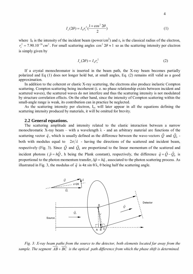

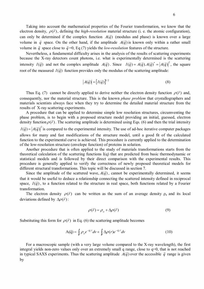


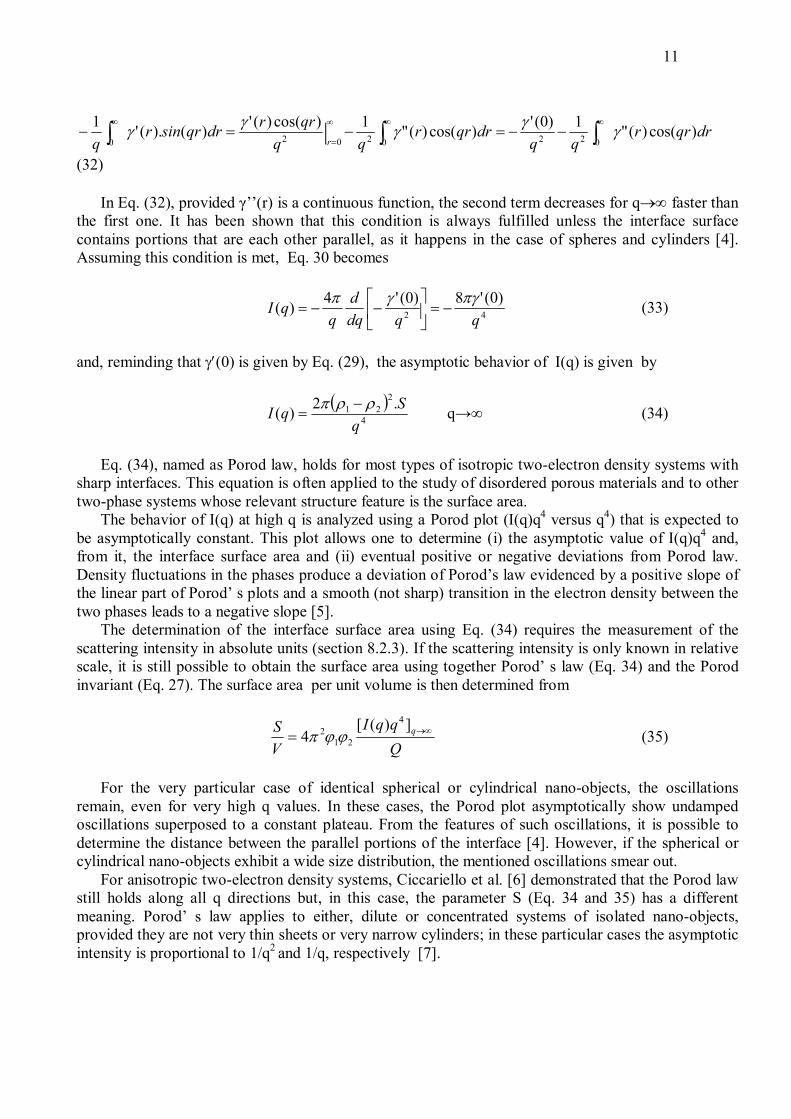


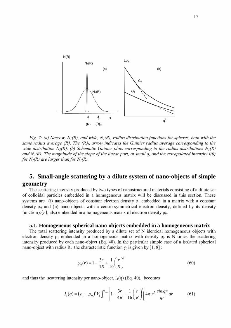
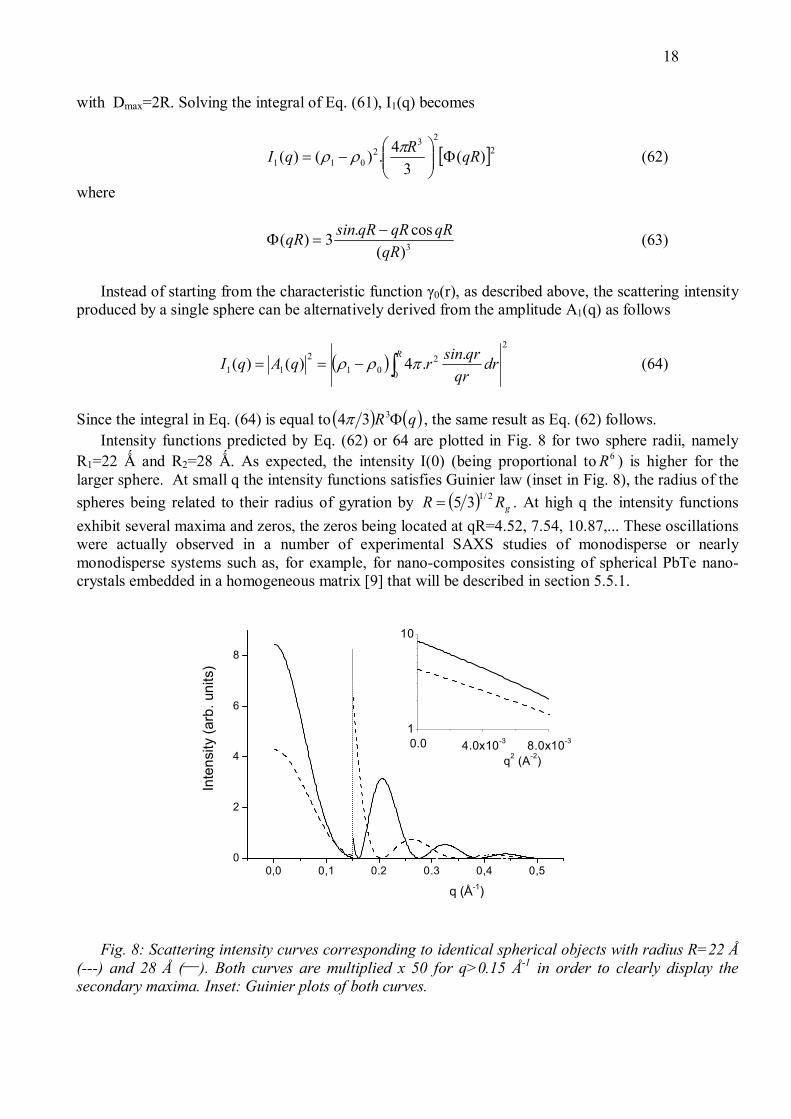
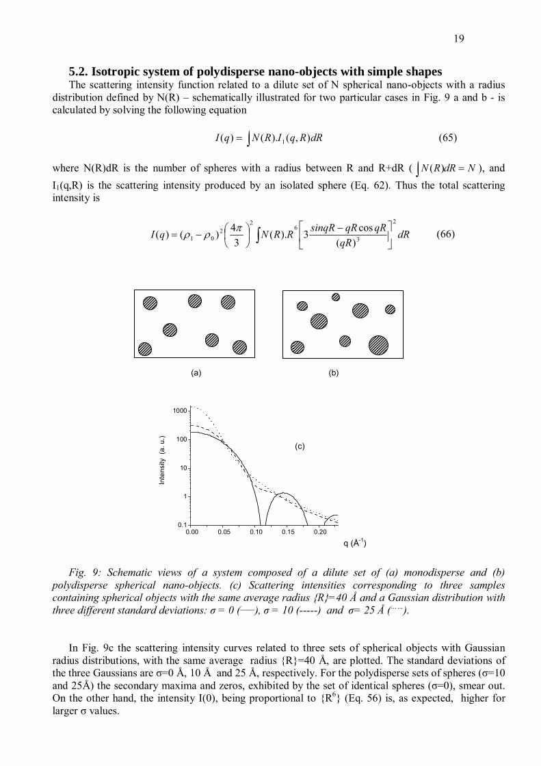


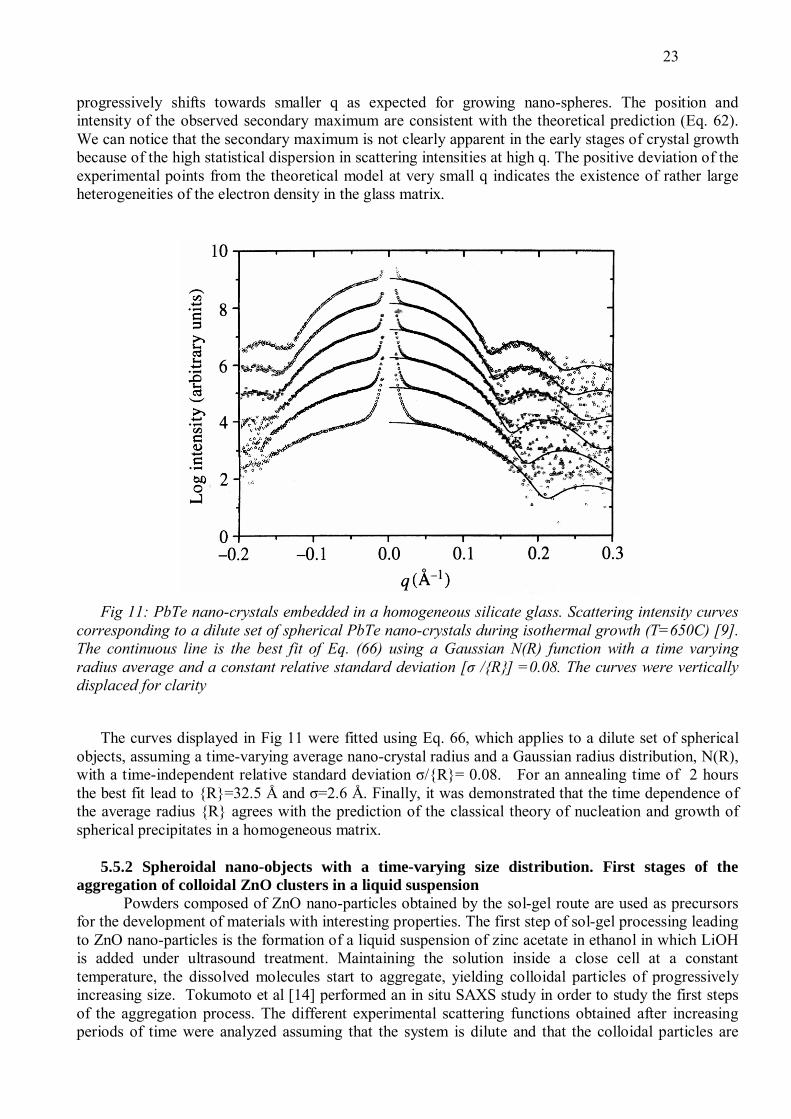


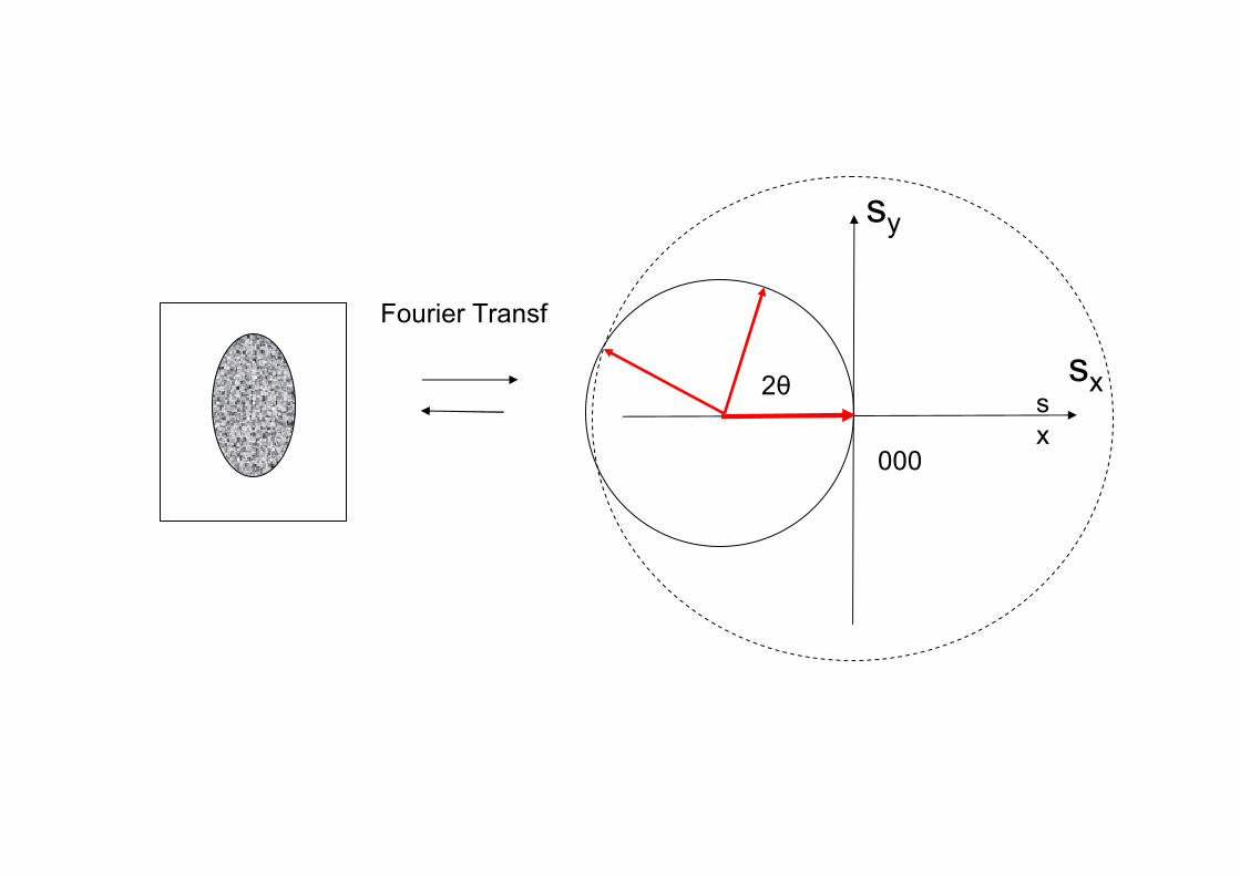

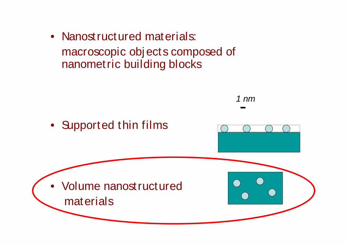
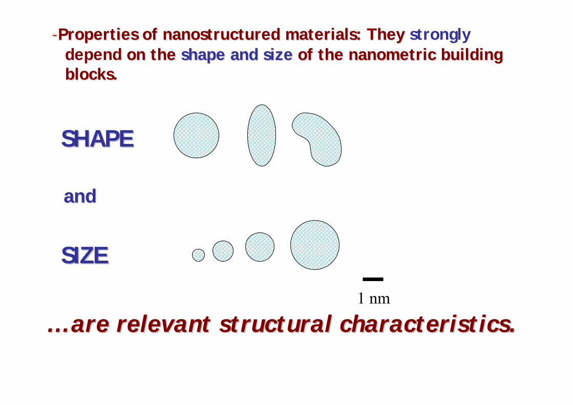


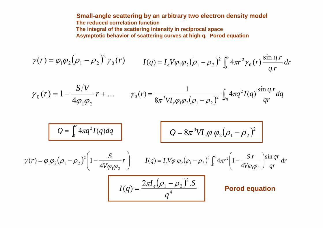


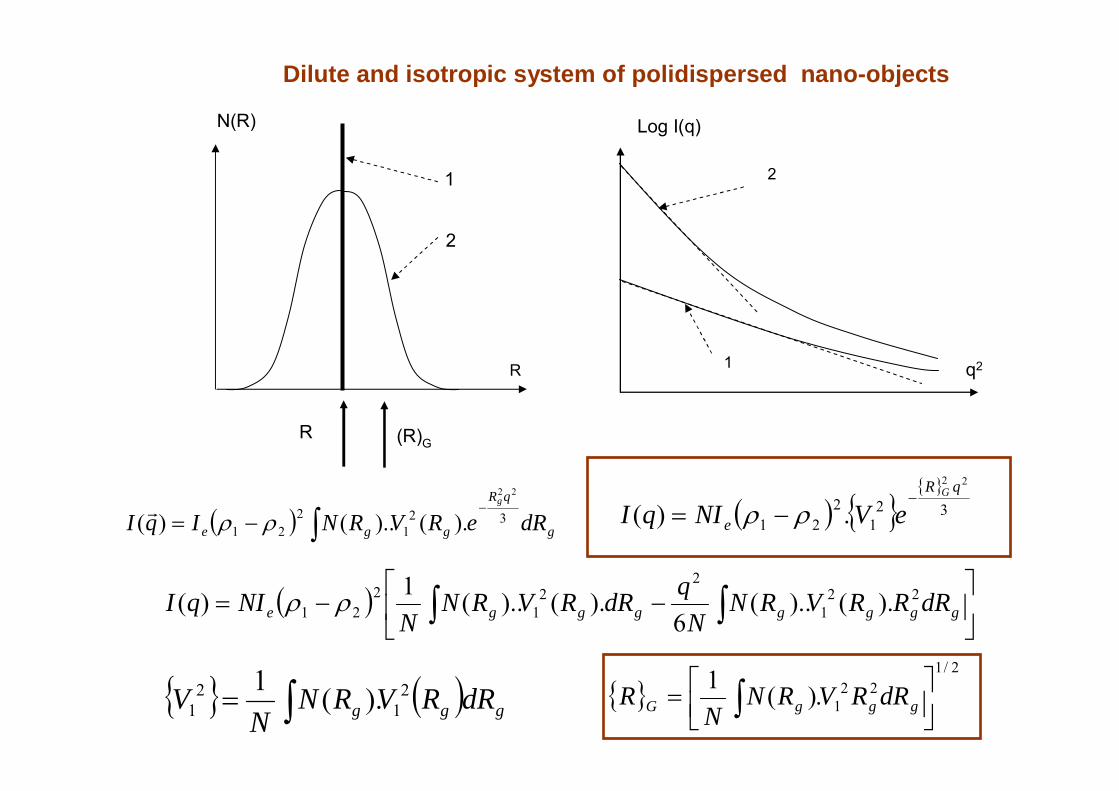


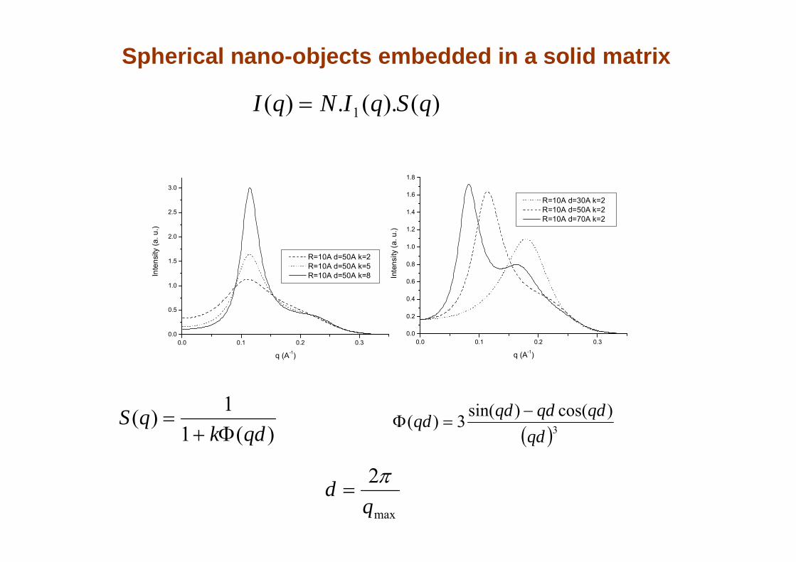


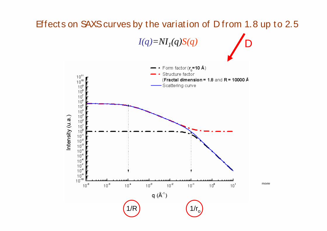


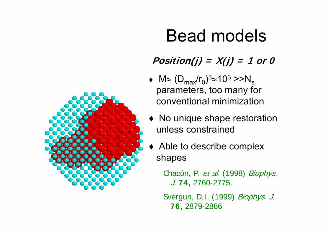


![Introduction to Linear Regression - Indico [Home]indico.ictp.it/event/a09161/session/2/contribution/1/material/0/0.pdf · Introduction to Linear Regression ... Regression Analysis:set](https://static.documents.pub/doc/80x56/5b7803f67f8b9a4c438e696d/introduction-to-linear-regression-indico-home-introduction-to-linear-regression.jpg)


