Università Politecnica delle Marche Facoltà di Ingegneria – Istituto di Idraulica ed Infrastrutture Viarie Andrea Grilli ADVANCED TESTING AND THEORETICAL EVALUATION OF BITUMINOUS MIXTURES FOR FLEXIBLE PAVEMENTS Portonovo, Ancona, Spring 2007 Portonovo, Ancona, Spring 2007 Ph.D. Coordinator: Prof. Felice A. Santagata Tutor: Prof. Amedeo Virgili Co-Tutor: Prof. Francesco Canestrari Dottorato di Ricerca in Strutture ed Infrastrutture VI ciclo – nuova sede
Transcript
Università Politecnica delle Marche Facoltà di Ingegneria – Istituto di Idraulica ed Infrastrutture Viarie
Andrea Grilli
ADVANCED TESTING AND
THEORETICAL EVALUATION OF BITUMINOUS MIXTURES FOR
FLEXIBLE PAVEMENTS
Portonovo, Ancona, Spring 2007Portonovo, Ancona, Spring 2007
Ph.D. Coordinator: Prof. Felice A. Santagata
Tutor: Prof. Amedeo Virgili
Co-Tutor: Prof. Francesco Canestrari
Dottorato di Ricerca in Strutture ed Infrastrutture VI ciclo – nuova sede
Dedicato ai miei genitori
We'd gather around all in a room fasten our belts engage in dialogue
We'd all slow down rest without guilt not lie without fear disagree sans judgment
We would stay and respond and expand and include and allow and forgive and enjoy and evolve and discern and
inquire and accept and admit and divulge and open and reach out and speak up
This is utopia this is my utopiaThis is my ideal my end in sight
Utopia this is my utopiaThis is my nirvana
My ultimate
We'd open our arms we'd all jump in We'd all coast down into safety nets
We would share and listen and support and welcome be propelled by passion not invest in outcomes
We would breathe and be charmed and amused by difference be gentle and make room for every emotion
We'd provide forums we'd all speak out We'd all be heard we'd all feel seen
We'd rise post-obstacle more defined more grateful We would heal be humbled and be unstoppable
We'd hold close and let go and know when to do which We'd release and disarm and stand up and feel safe
This is utopia this is my utopiaThis is my ideal my end in sight
Utopia this is my utopiaThis is my nirvana
My ultimate
Alanis Morissette, Under rug swept, 2002.
Spiaggia di Mezzavalle, Ancona, Summer 2007
We'd gather around all in a room fasten our belts engage in dialogue
We'd all slow down rest without guilt not lie without fear disagree sans judgment
We would stay and respond and expand and include and allow and forgive and enjoy and evolve and discern and
inquire and accept and admit and divulge and open and reach out and speak up
This is utopia this is my utopiaThis is my ideal my end in sight
Utopia this is my utopiaThis is my nirvana
My ultimate
We'd open our arms we'd all jump in We'd all coast down into safety nets
We would share and listen and support and welcome be propelled by passion not invest in outcomes
We would breathe and be charmed and amused by difference be gentle and make room for every emotion
We'd provide forums we'd all speak out We'd all be heard we'd all feel seen
We'd rise post-obstacle more defined more grateful We would heal be humbled and be unstoppable
We'd hold close and let go and know when to do which We'd release and disarm and stand up and feel safe
This is utopia this is my utopiaThis is my ideal my end in sight
Utopia this is my utopiaThis is my nirvana
My ultimate
Alanis Morissette, Under rug swept, 2002.
Spiaggia di Mezzavalle, Ancona, Summer 2007
Table of contents
Table of contents
List of tables ................................................................................. 5 List of figures................................................................................ 7 Abstract....................................................................................... 13 Sommario.................................................................................... 15 Acknowledgments ...................................................................... 17
3. Experimental program – Part I ....................................................... 43
3.1 Specimen preparation ........................................................... 43 3.2 Shear test program ................................................................ 46 3.3 Four point bending test program........................................... 48
4. Test equipments – Part I................................................................. 49
Advanced Testing And Theoretical Evaluation Of Bituminous Mixtures For Flexible Pavements
4.2 ASTRA test device ............................................................... 52 4.3 Four point bending test ......................................................... 62
5. Result analysis................................................................................ 65
5.2 Four point bending test ......................................................... 78 5.2.1 Deflection control test ................................................ 78 5.2.2 Load control test......................................................... 82 5.2.3 Integrated fatigue model for LCT .............................. 89
Part II................................................................................................ 103
Influence of water and temperature on asphalt mixtures ................. 103
6. Literature review – Part II ............................................................ 105
6.3 Cohesion theory .................................................................. 109 6.4 Review of test methods....................................................... 109
6.4.1 Effect of Water on Bituminous-Coated Aggregate Using Boiling Water (ASTM D 3625-96) ........................ 110 6.4.2 Determination of the affinity between aggregate and bitumen (EN 12697-11) .................................................... 111
2
Table of contents
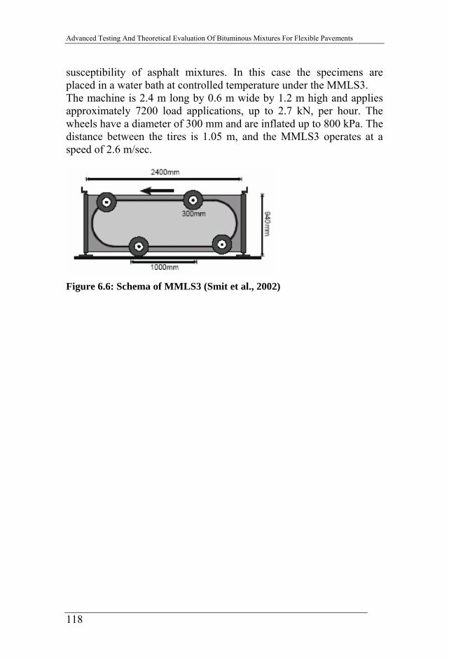
6.4.3 Net adsorption test (SHRP Designation M-001)...... 111 6.4.4 Marshall stability test (AASHTO T245).................. 112 6.4.5 Modified Lottman procedure (AASHTO T283) ...... 112 6.4.6 Effect of Moisture on Asphalt Concrete Paving Mixtures (ASTM D 4867)................................................. 113 6.4.7 Environmental Conditioning System (ECS) ............ 113 6.4.8 Nottingham Asphalt Tester ...................................... 115 6.4.9 Saturation Ageing Tensile Stiffness (SATS) test..... 115 6.4.10 Asphalt Pavement Analyzer................................... 116 6.4.11 Hamburg Wheel-Tracking Device ......................... 117 6.4.12 Model Mobile Load Simulator............................... 117
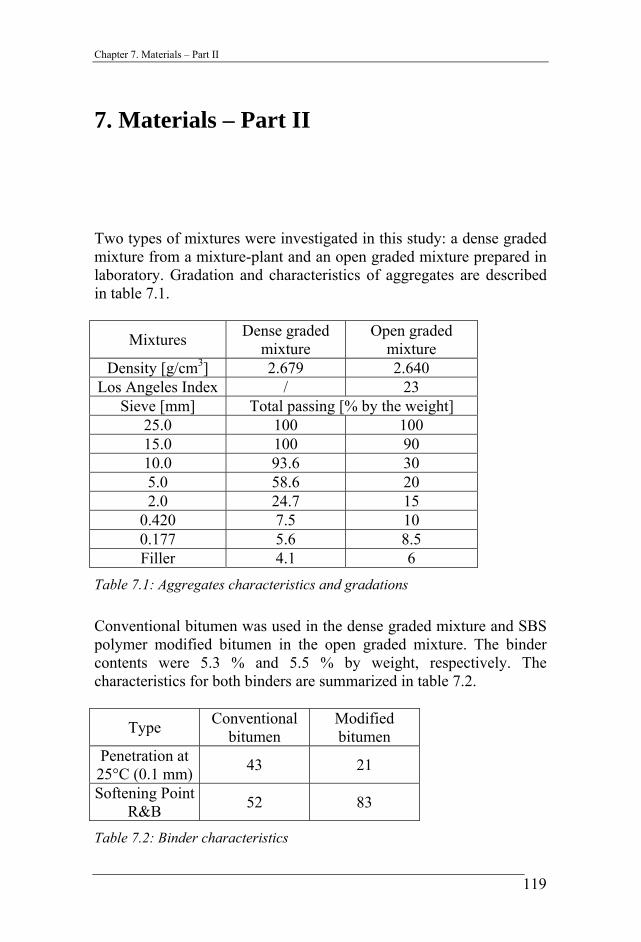
7. Materials – Part II......................................................................... 119
8. Experimental program – Part II.................................................... 121
9. Test methods and procedures – Part II ......................................... 125
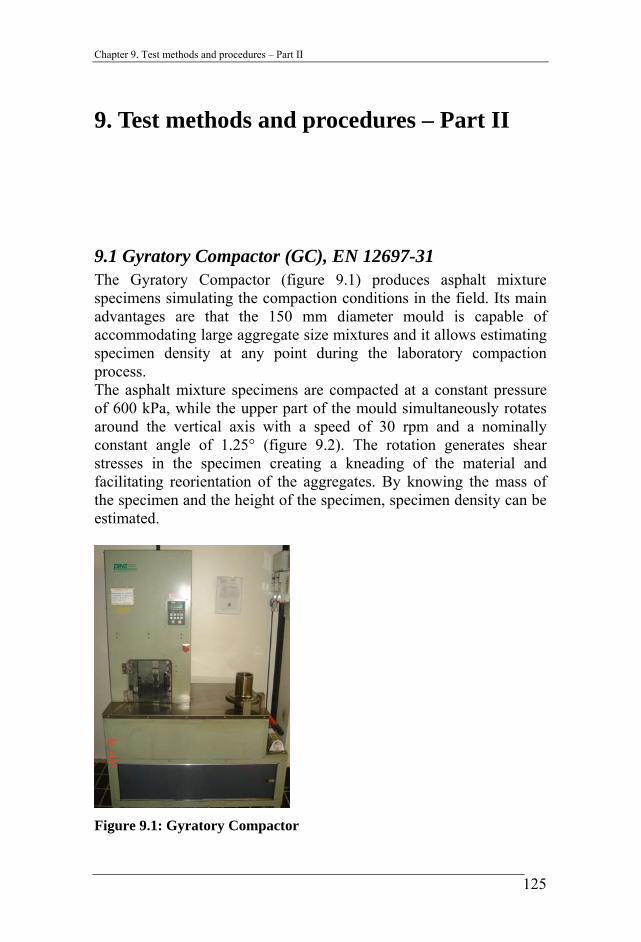
9.1 Gyratory Compactor (GC), EN 12697-31 .......................... 125 9.2 Coaxial Shear Test (CAST) ................................................ 126 9.3 Indirect tensile Test (IDT), ASTM D4867 ......................... 130 9.4 Cantabro test equipment, EN 12697-17.............................. 131
10. Result analysis – Part II.............................................................. 133
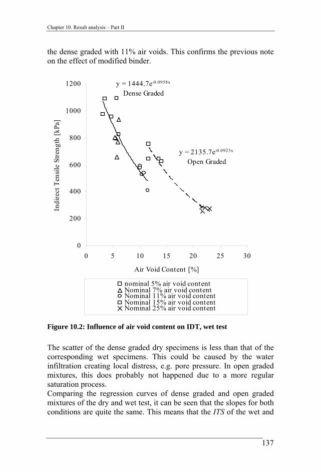
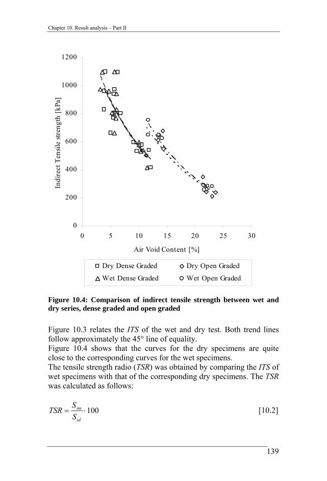
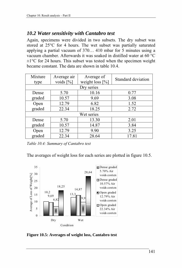
10.1 Water sensitivity with IDT ............................................... 133 10.2 Water sensitivity with Cantabro test................................. 141 10.3 Water sensitivity with CAST............................................ 144
10.3.1 Experimental output ............................................... 144 10.3.2 Statistical analysis .................................................. 147 10.3.3 Water sensitivity index........................................... 148 10.3.4 Master curve and model parameters analysis before and after dry and wet fatigue testing ................................. 157 10.3.5 Model for the first phase of fatigue test with or without temperature cycles ............................................... 162 10.3.6 Generalized model for fatigue test with or without temperature cycles............................................................. 169 10.3.7 Fatigue performance evaluation by means of the generalized model ............................................................. 174
3
Advanced Testing And Theoretical Evaluation Of Bituminous Mixtures For Flexible Pavements
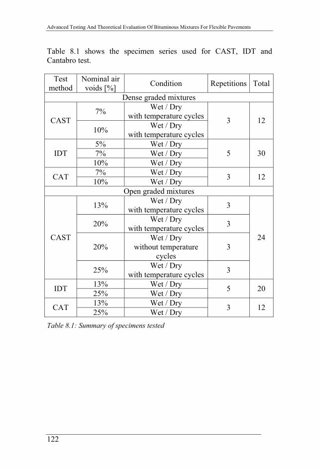
Table 8.1: Summary of specimens tested......................................... 122
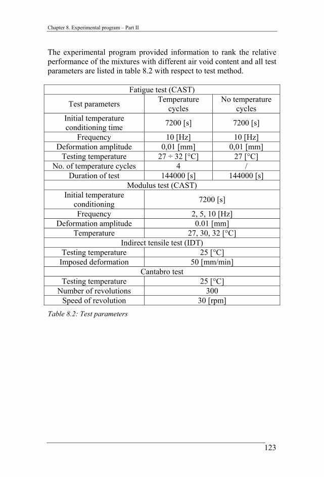
Table 8.2: Test parameters ............................................................... 123
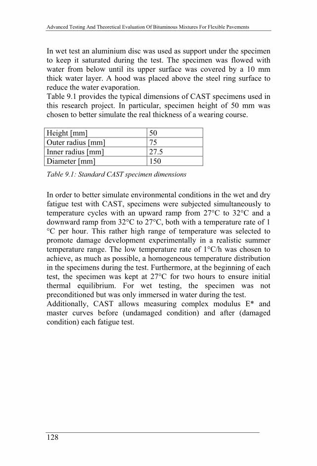
Table 9.1: Standard CAST specimen dimensions............................ 128
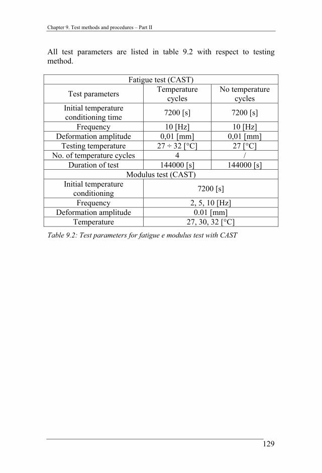
Table 9.2: Test parameters for fatigue e modulus test with CAST .. 129
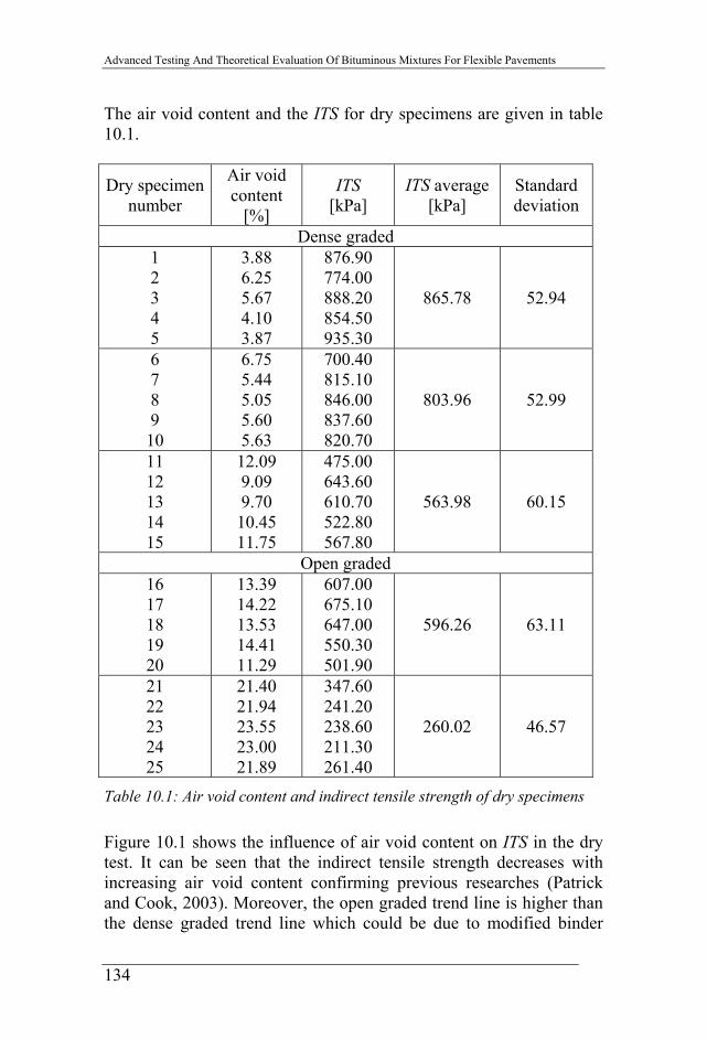
Table 10.1: Air void content and indirect tensile strength of dry specimens ......................................................................................... 134
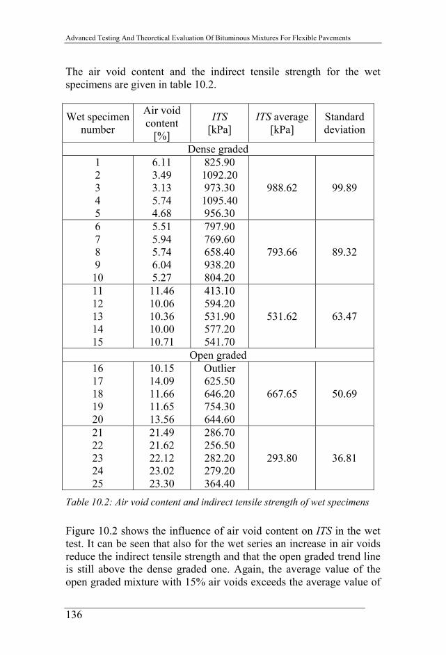
Table 10.2: Air void content and indirect tensile strength of wet specimens ......................................................................................... 136
Table 10.3: Tensile strength radio for each series............................ 140
Table 10.4: Summary of Cantabro test............................................. 141
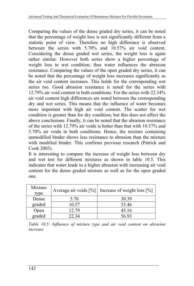
Table 10.5: Influence of mixture type and air void content on abrasion increase............................................................................................. 142
5
Advanced Testing And Theoretical Evaluation Of Bituminous Mixtures For Flexible Pavements
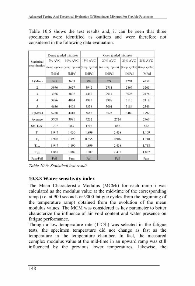
Table 10.6: Statistical test result ...................................................... 148
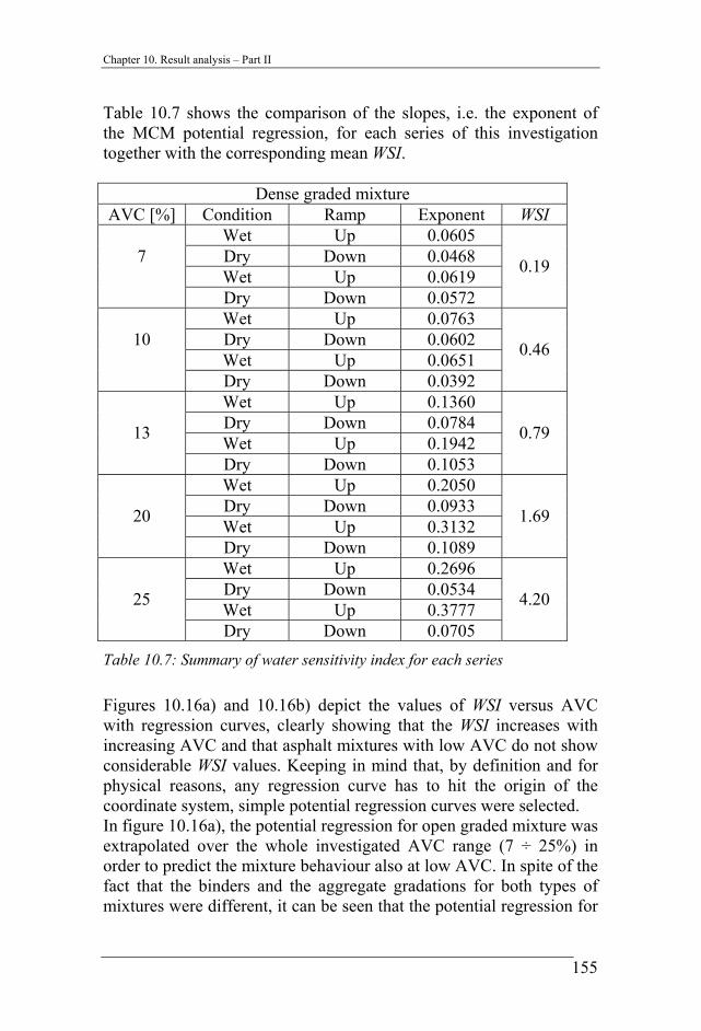
Table 10.7: Summary of water sensitivity index for each series ..... 155
Table 10.8: Parameters for SLS model for each specimen .............. 159
Table 10.9: Parameters for SLS model for each specimen .............. 161
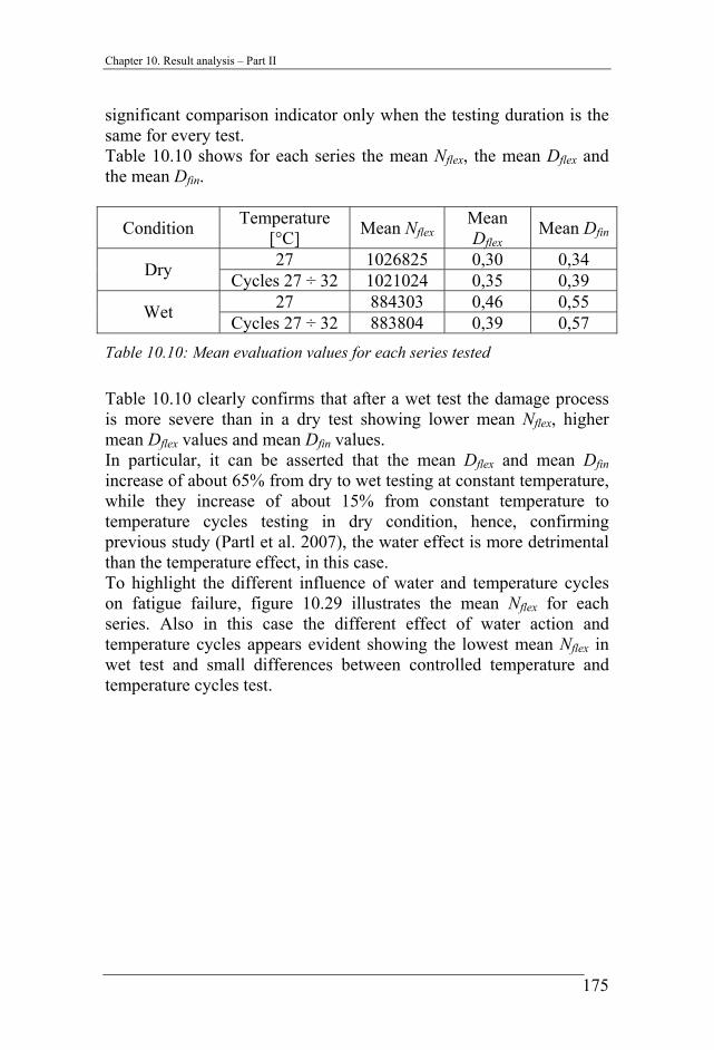
Table 10.10: Mean evaluation values for each series tested ............ 175
6
List of figures
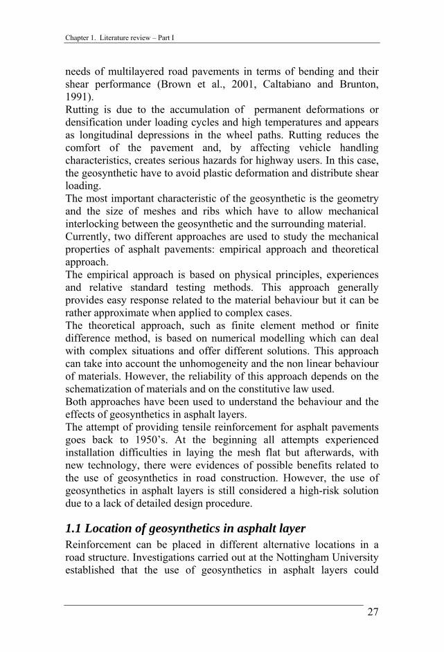
List of figures Figure 1.1: Pavement cross-sections (Brown et al., 2001)................. 28
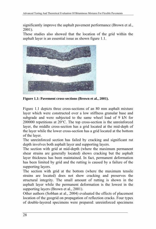
Figure 1.2: Behaviour of reinforced and unreinforced beam under repeated loading (Sobhan at al., 2004). .............................................. 29
Figure 1.4: Repeated load shear test for interfaces (Brown et al., 2001)................................................................................................... 32
Figure 1.5: Development of permanent deformation (Brown et al., 1985)................................................................................................... 33
Figure 1.6: Comparison between reinforced and unreinforced slab (Brown et al., 1985)............................................................................ 33
Figure 1.7: Fatigue curve for reinforced and unreinforced beam (Brown et al., 1985)............................................................................ 34
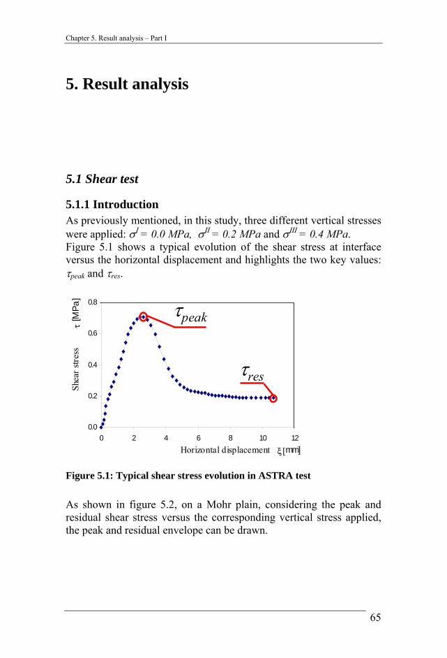
Figure 5.1: Typical shear stress evolution in ASTRA test ................. 65
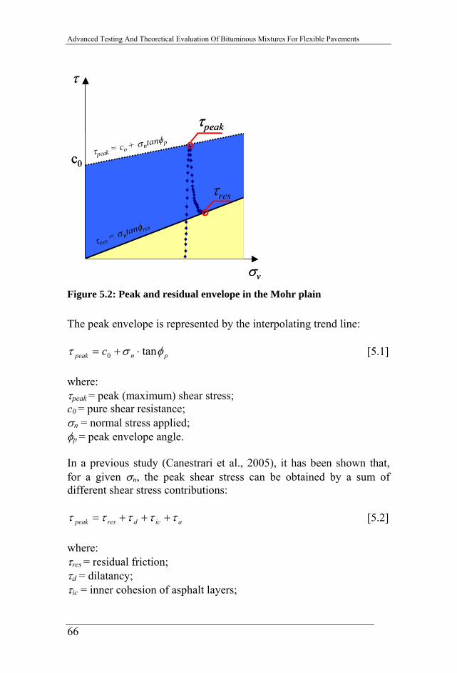
Figure 5.2: Peak and residual envelope in the Mohr plain................. 66
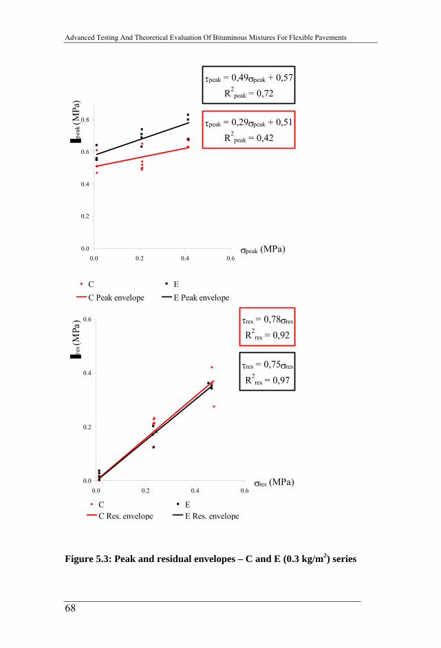
Figure 5.3: Peak and residual envelopes – C and E (0.3 kg/m2) series............................................................................................................ 68
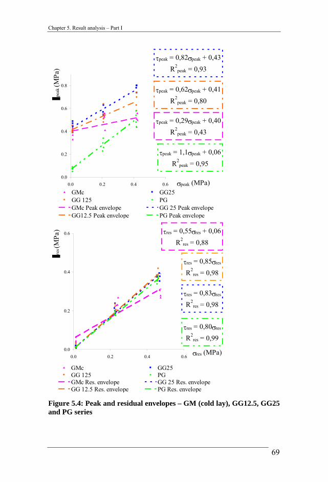
Figure 5.4: Peak and residual envelopes – GM (cold lay), GG12.5, GG25 and PG series ........................................................................... 69
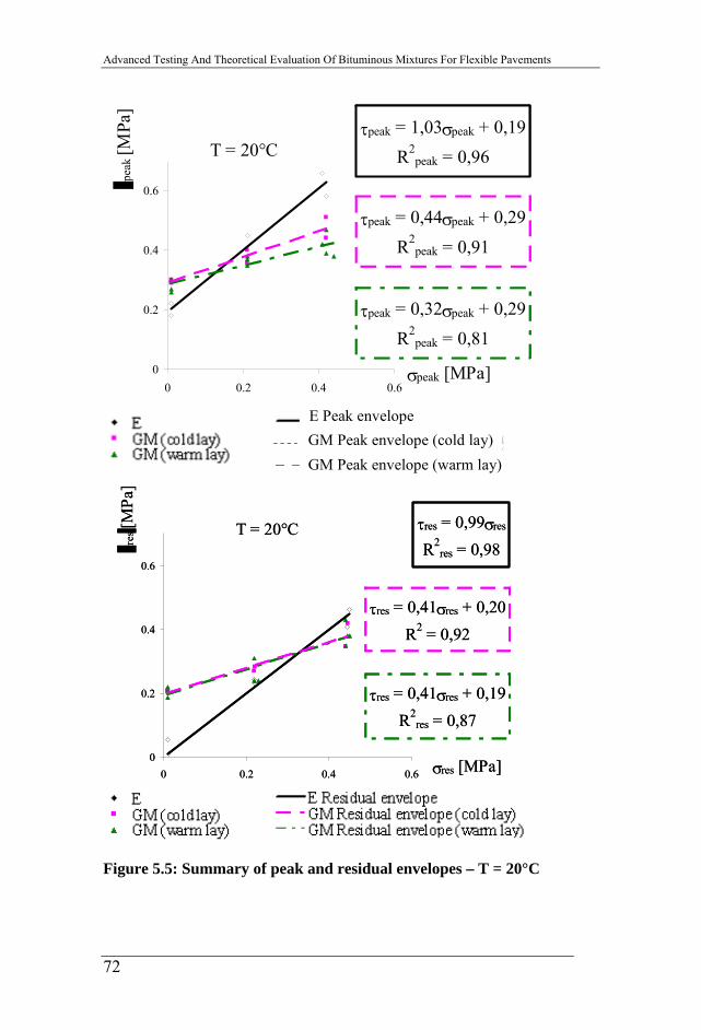
Figure 5.5: Summary of peak and residual envelopes – T = 20°C .... 72
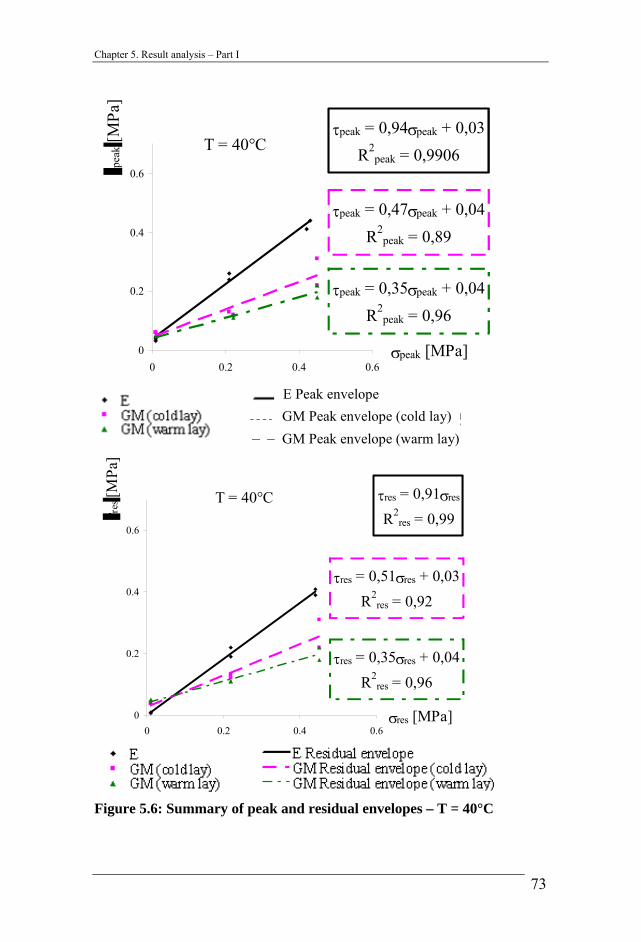
Figure 5.6: Summary of peak and residual envelopes – T = 40°C .... 73
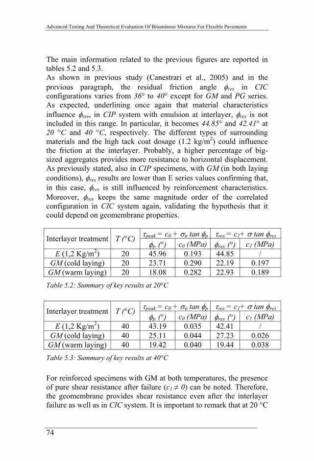
Figure 5.7: Influence of temperature on φpeak – E (1.2 kg/m2) series. 76
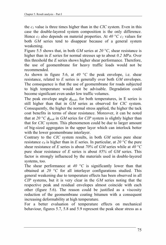
Figure 5.8: Influence of temperature on φpeak – GM series ................ 76
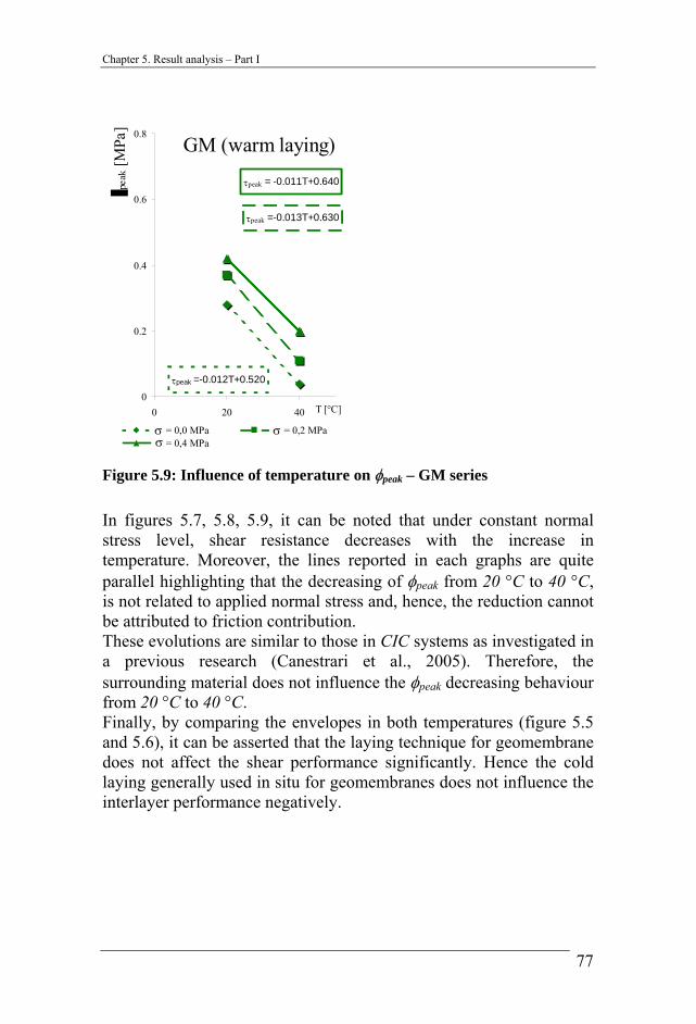
Figure 5.9: Influence of temperature on φpeak – GM series ................ 77
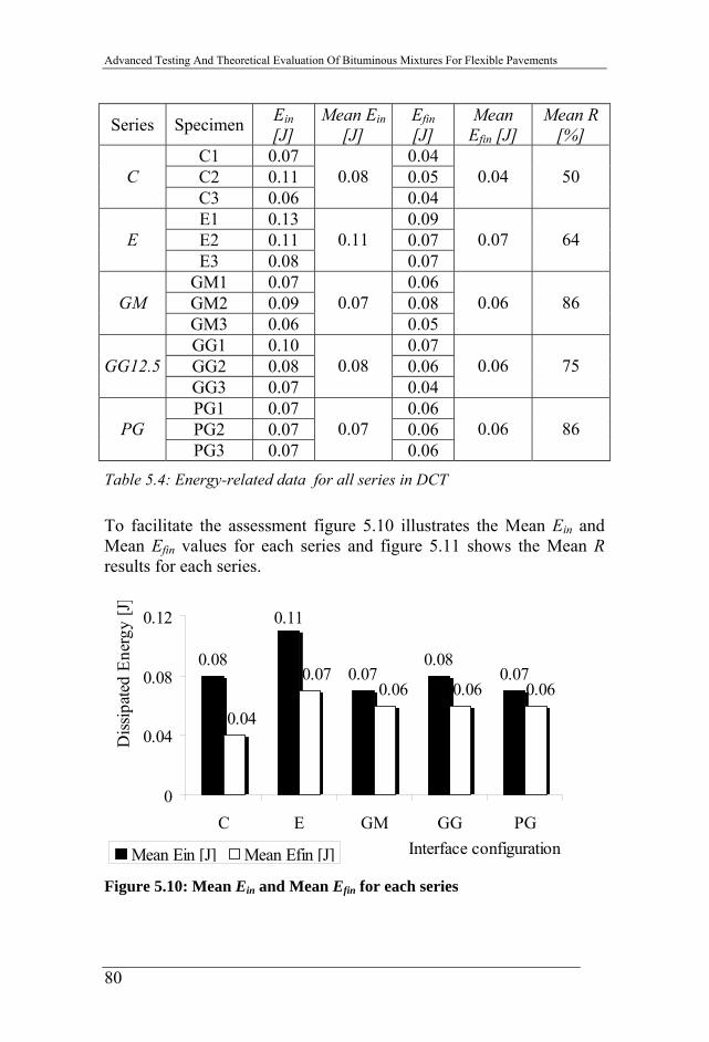
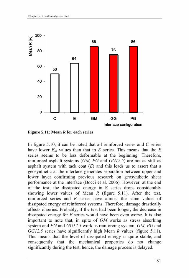
Figure 5.10: Mean Ein and Mean Efin for each series ......................... 80
Figure 5.11: Mean R for each series................................................... 81
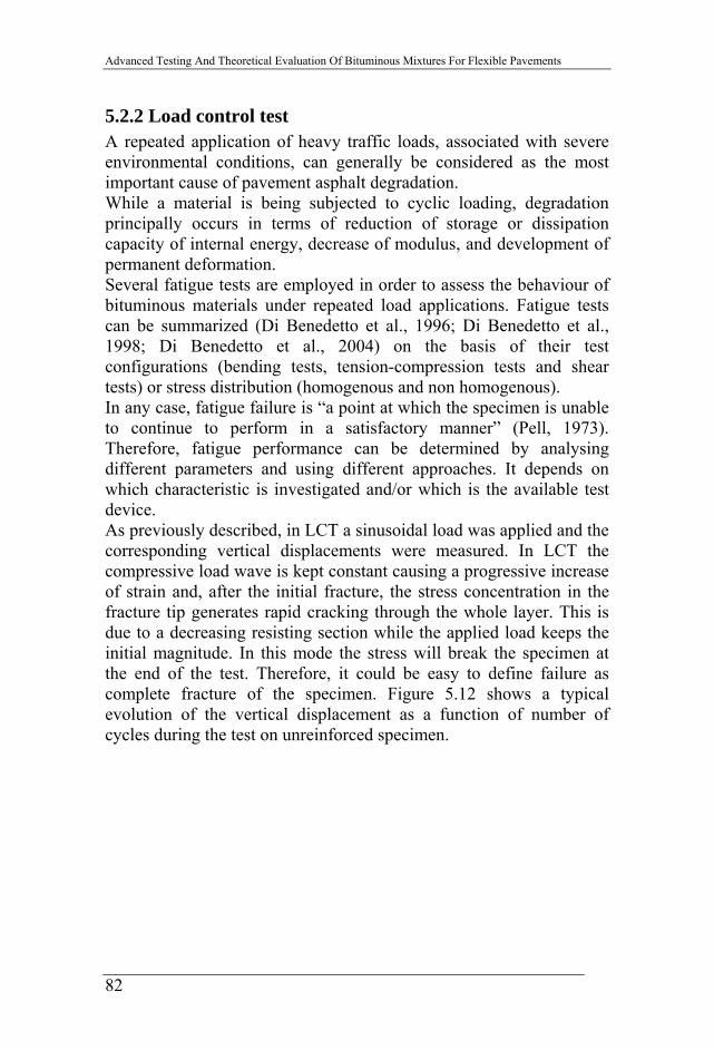
Figure 5.12: Vertical displacement versus number of cycles during a typical LCT ........................................................................................ 83
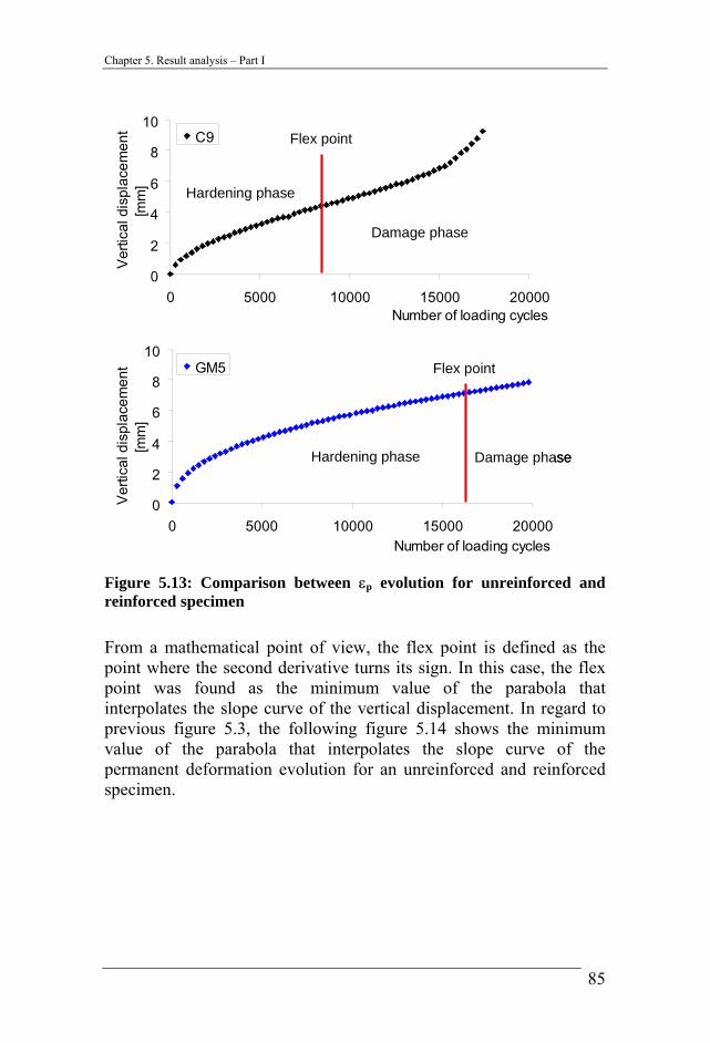
Figure 5.13: Comparison between εp evolution for unreinforced and reinforced specimen ........................................................................... 85
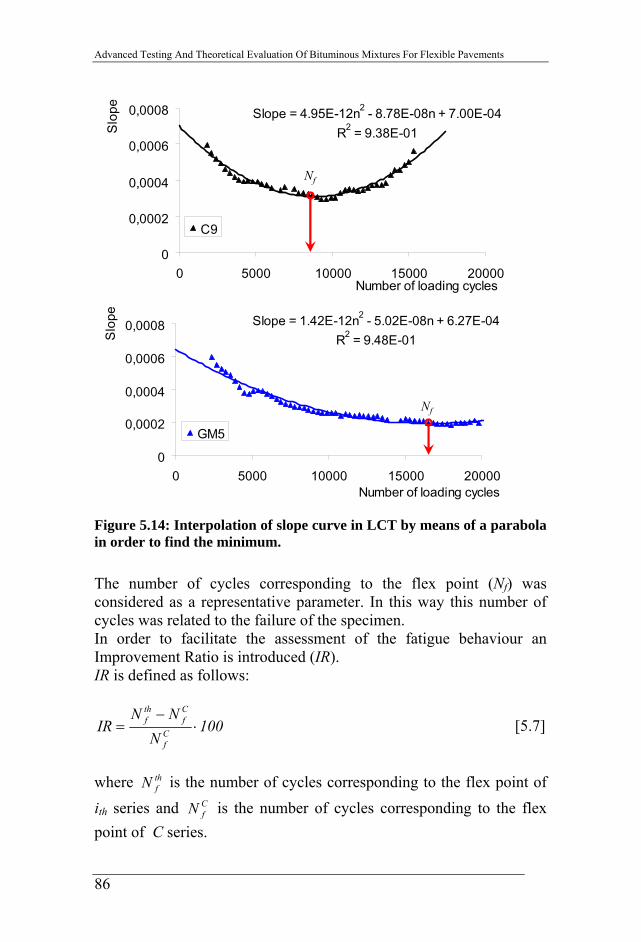
Figure 5.14: Interpolation of slope curve in LCT by means of a parabola in order to find the minimum............................................... 86
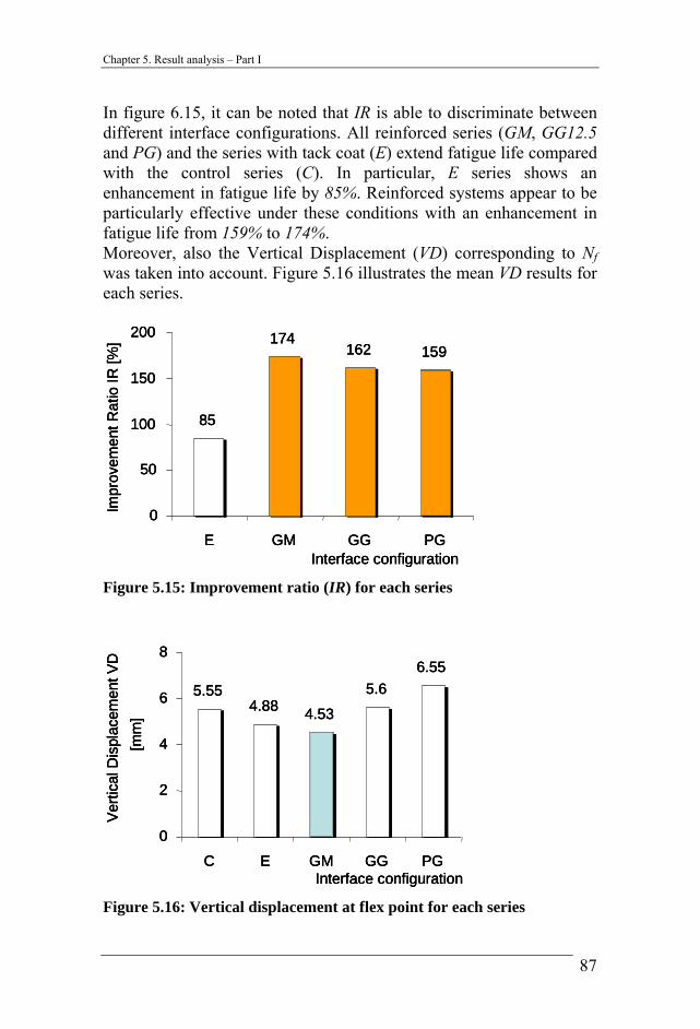
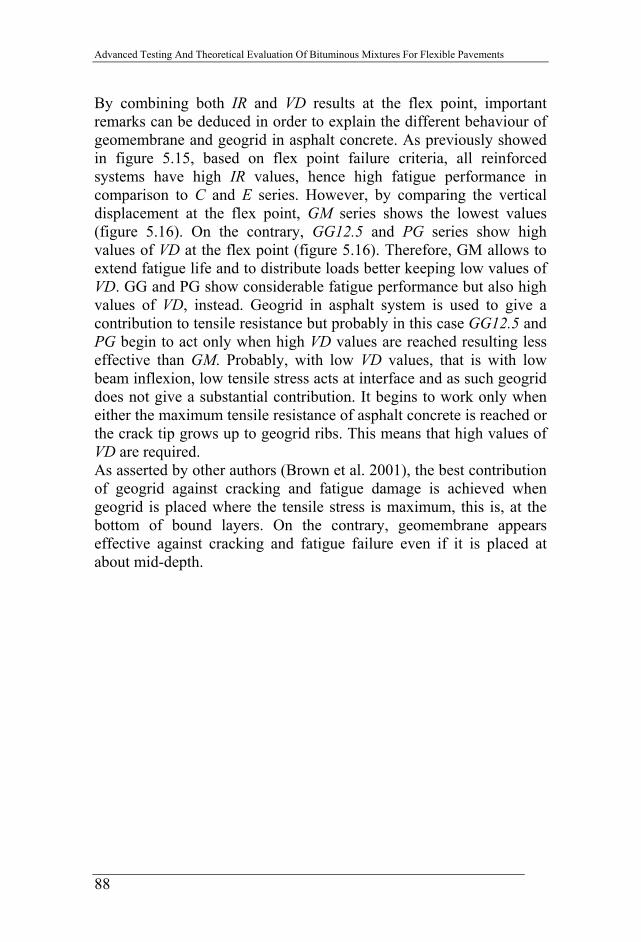
Figure 5.15: Improvement ratio (IR) for each series.......................... 87
Figure 5.16: Vertical displacement at flex point for each series ........ 87
8
List of figures
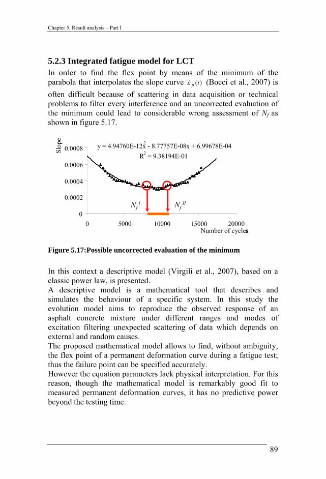
Figure 5.17:Possible uncorrected evaluation of the minimum........... 89
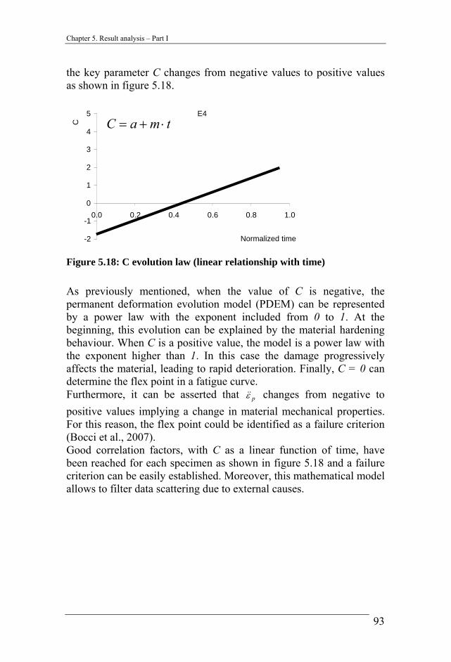
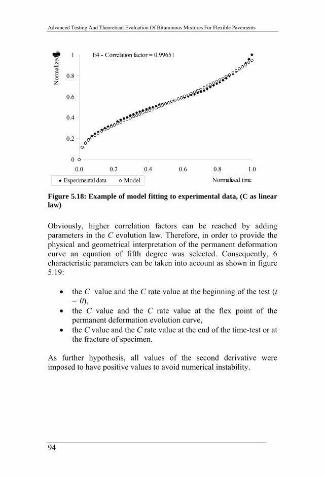
Figure 5.18: C evolution law (linear relationship with time)............. 93
Figure 5.18: Example of model fitting to experimental data, (C as linear law)........................................................................................... 94
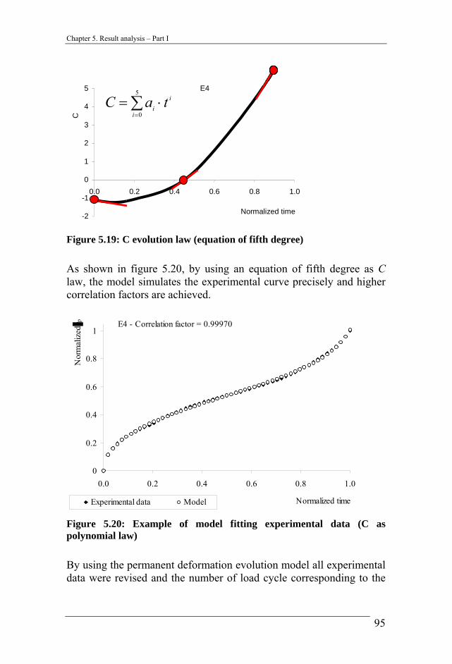
Figure 5.19: C evolution law (equation of fifth degree) .................... 95
Figure 5.20: Example of model fitting experimental data (C as polynomial law).................................................................................. 95
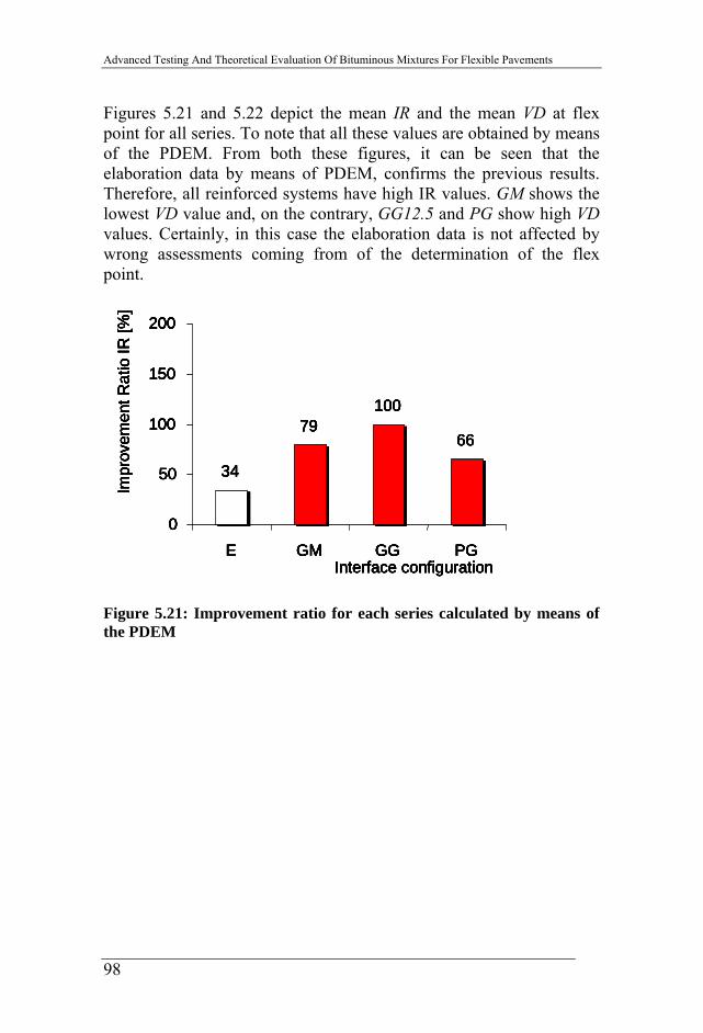
Figure 5.21: Improvement ratio for each series calculated by means of the PDEM........................................................................................... 98
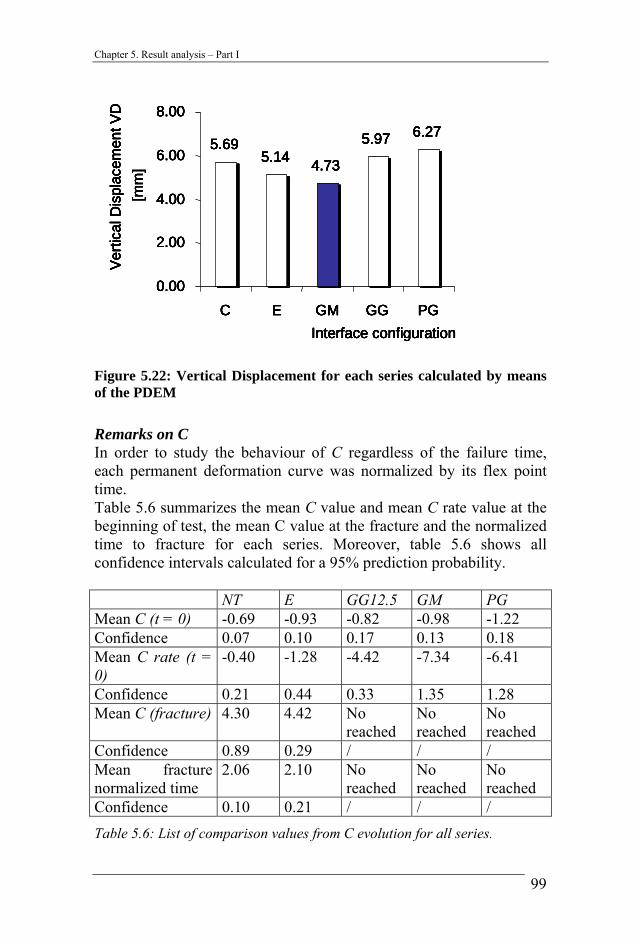
Figure 5.22: Vertical Displacement for each series calculated by means of the PDEM ........................................................................... 99
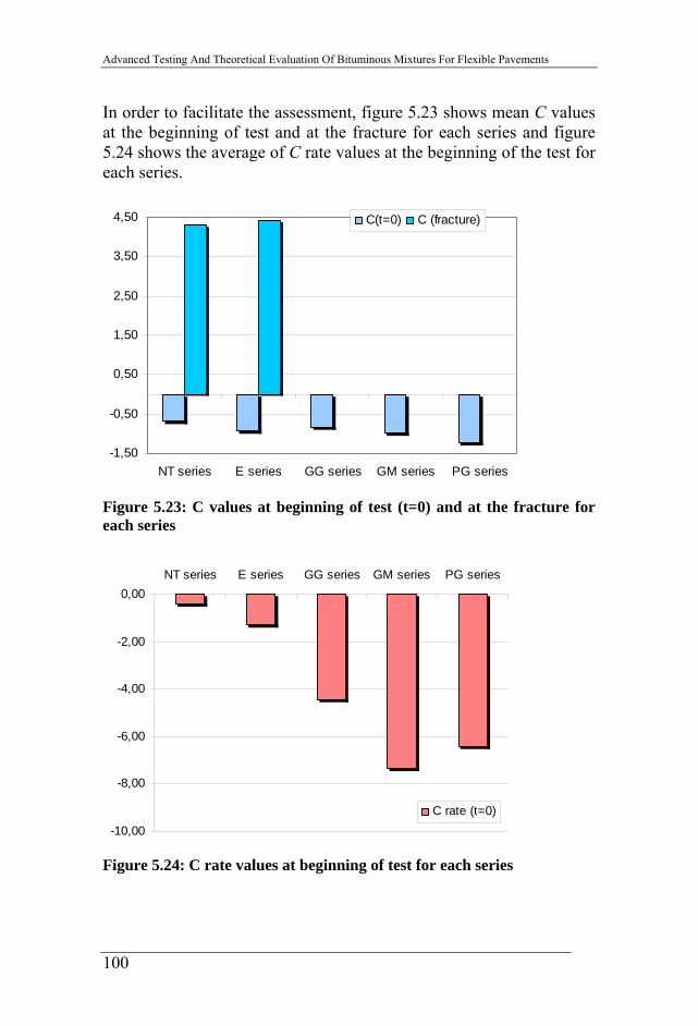
Figure 5.23: C values at beginning of test (t=0) and at the fracture for each series ........................................................................................ 100
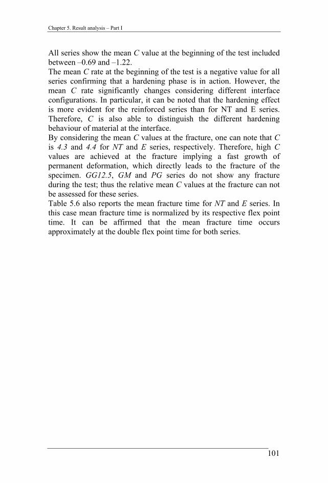
Figure 5.24: C rate values at beginning of test for each series......... 100
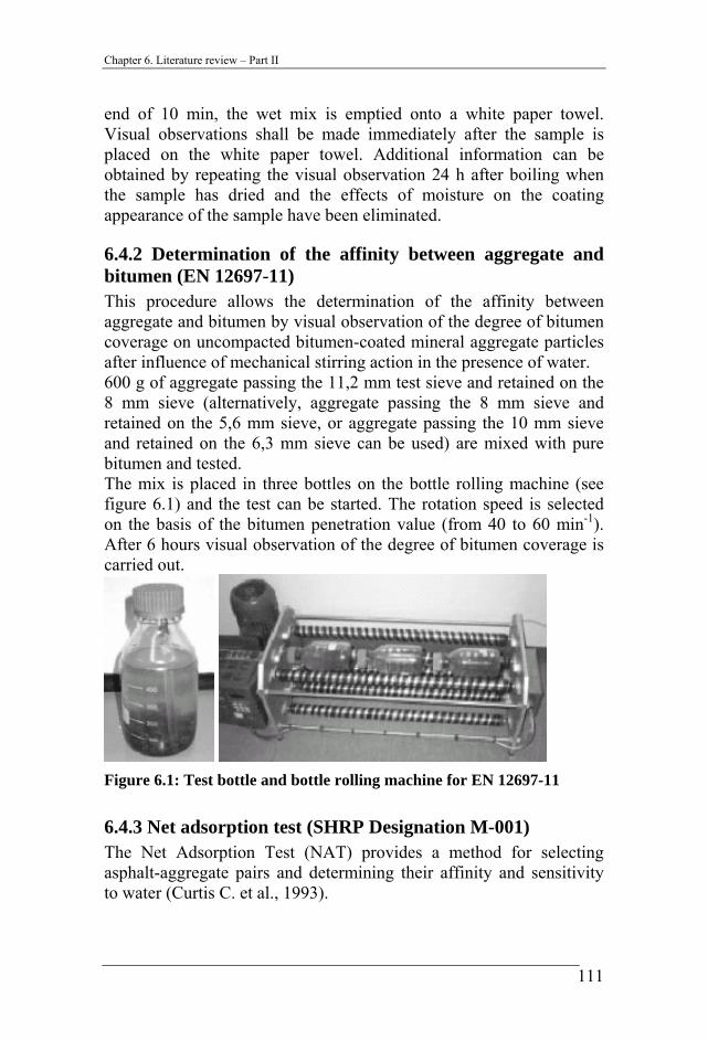
Figure 6.1: Test bottle and bottle rolling machine for EN 12697-11111
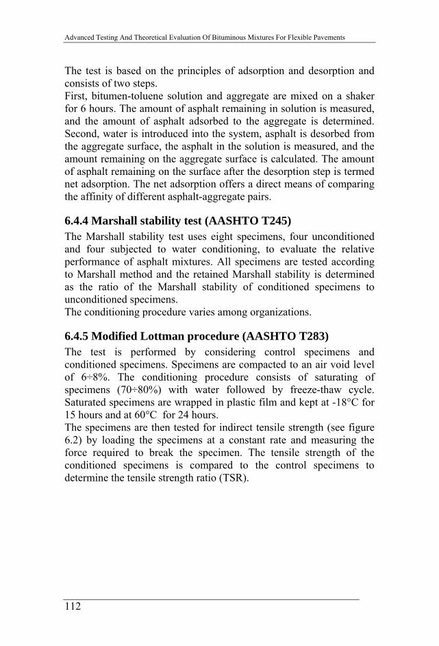
Figure 6.2: Specimen in testing frame ............................................. 113
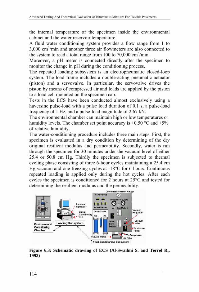
Figure 6.3: Schematic drawing of ECS (Al-Swailmi S. and Terrel R., 1992)................................................................................................. 114
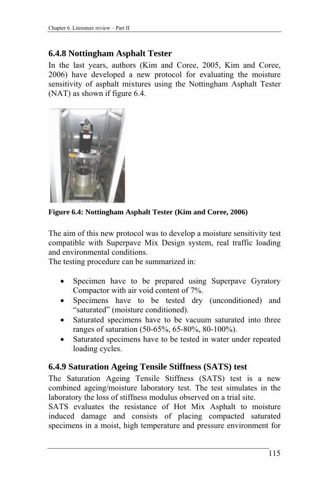
Figure 6.4: Nottingham Asphalt Tester (Kim and Coree, 2006)...... 115
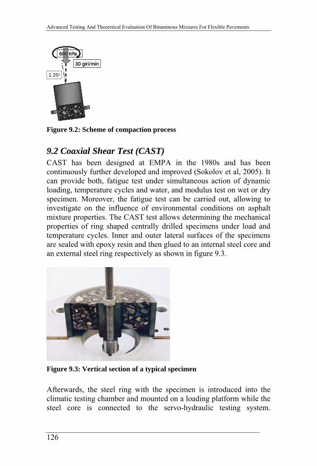
Figure 9.2: Scheme of compaction process...................................... 126
Figure 9.3: Vertical section of a typical specimen ........................... 126
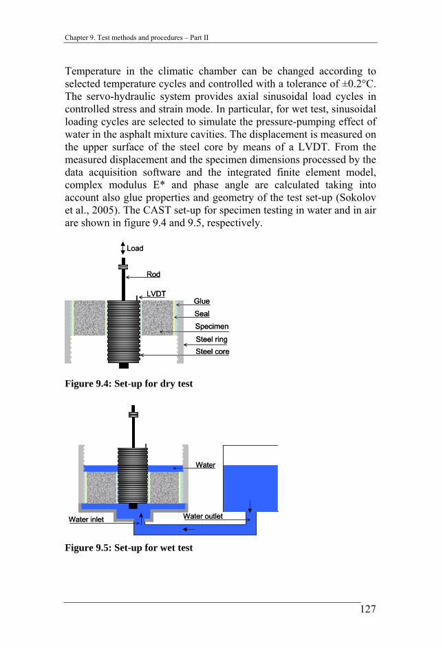
Figure 9.4: Set-up for dry test .......................................................... 127
Figure 9.5: Set-up for wet test.......................................................... 127
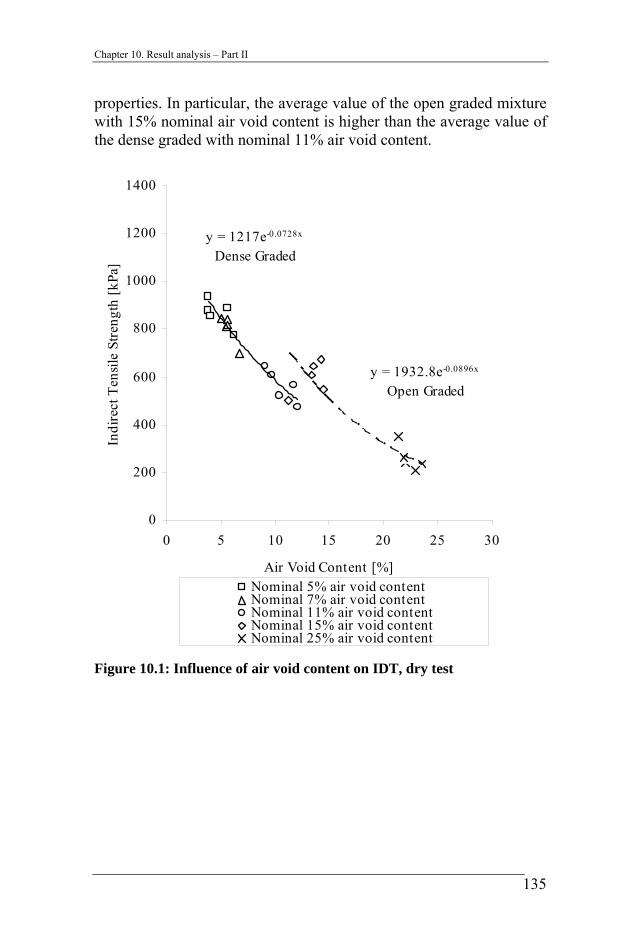
Figure 10.1: Influence of air void content on IDT, dry test ............. 135
Figure 10.2: Influence of air void content on IDT, wet test............. 137
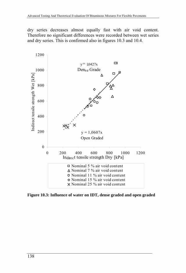
Figure 10.3: Influence of water on IDT, dense graded and open graded.......................................................................................................... 138
9
Advanced Testing And Theoretical Evaluation Of Bituminous Mixtures For Flexible Pavements
Figure 10.4: Comparison of indirect tensile strength between wet and dry series, dense graded and open graded ........................................ 139
Figure 10.5: Averages of weight loss, Cantabro test........................ 141
Figure 10.6: Rate of weight loss....................................................... 143
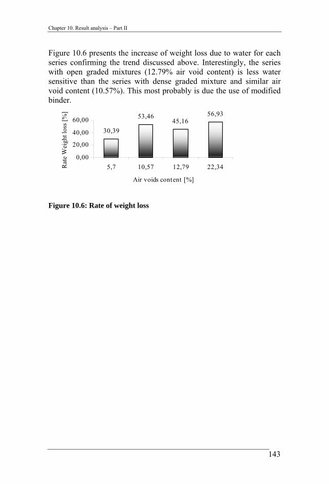
Figure 10.7: Mean evolution of modulus E* and phase angle in a dry test (25% AVC)................................................................................ 144
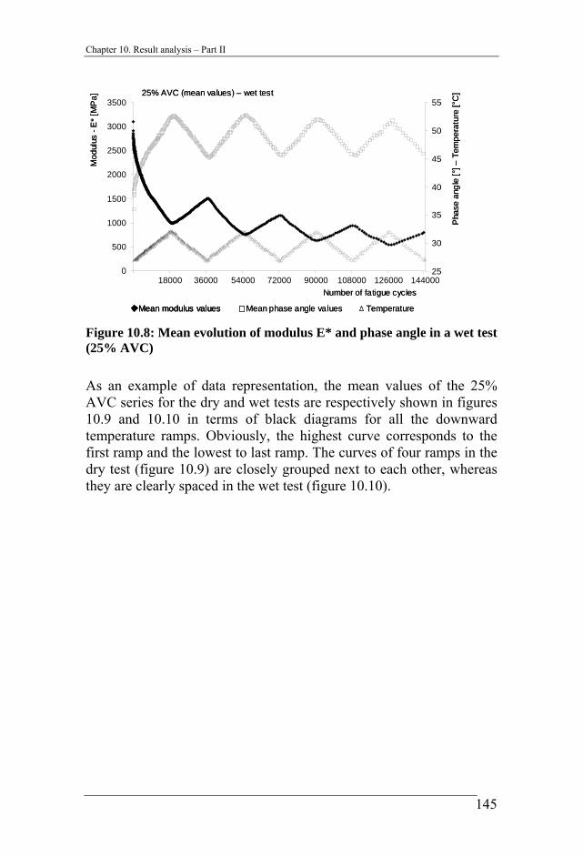
Figure 10.8: Mean evolution of modulus E* and phase angle in a wet test (25% AVC)................................................................................ 145
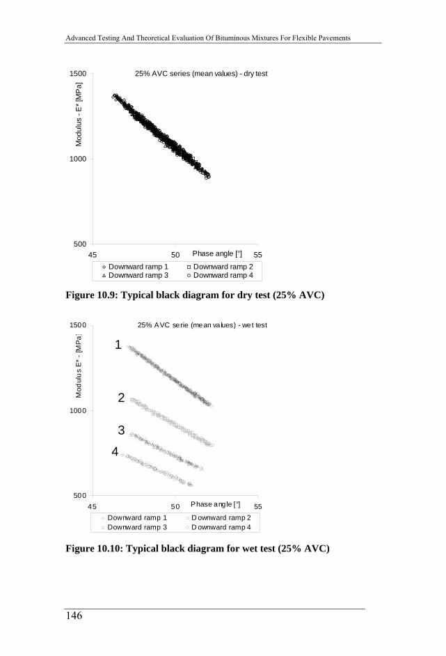
Figure 10.9: Typical black diagram for dry test (25% AVC) .......... 146
Figure 10.10: Typical black diagram for wet test (25% AVC)........ 146
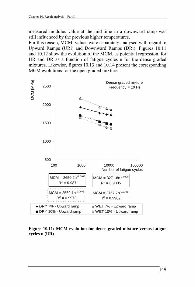
Figure 10.11: MCM evolution for dense graded mixture versus fatigue cycles n (UR).................................................................................... 149
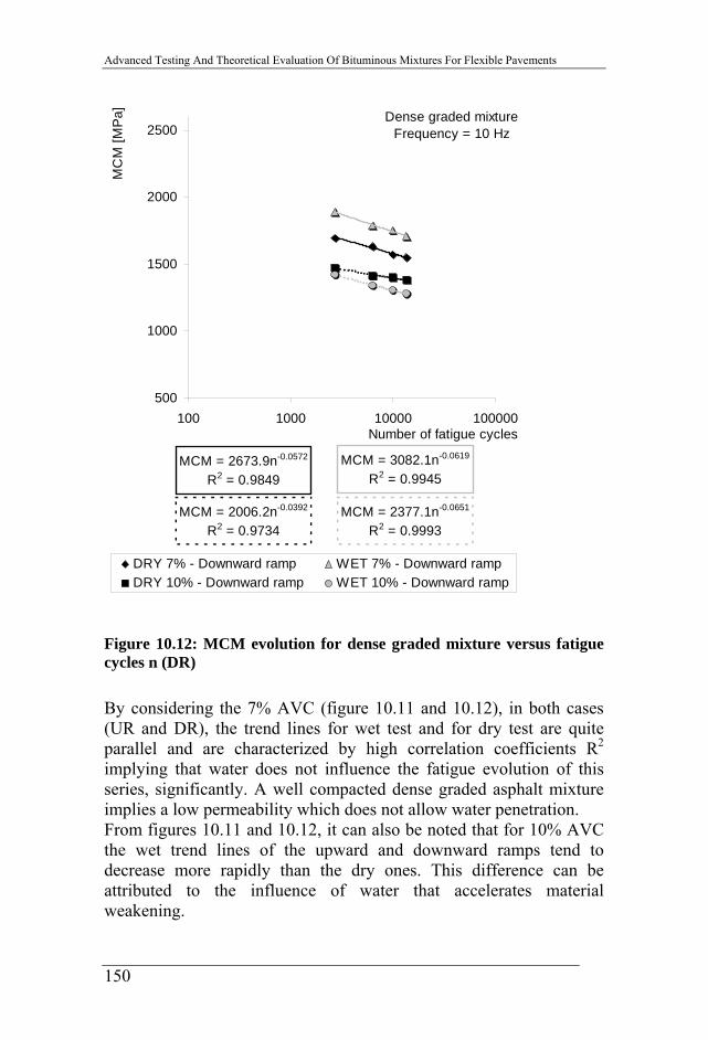
Figure 10.12: MCM evolution for dense graded mixture versus fatigue cycles n (DR).................................................................................... 150
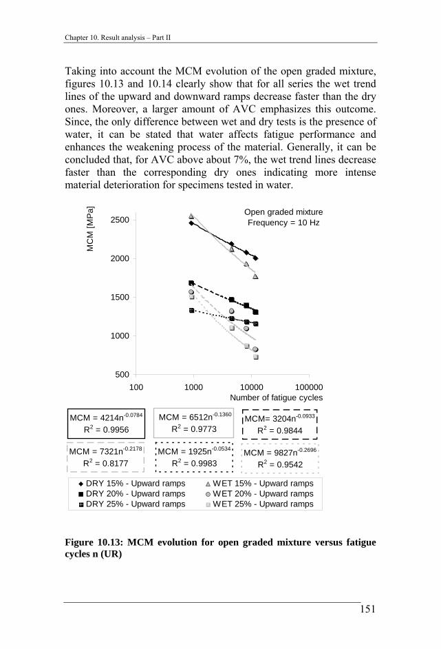
Figure 10.13: MCM evolution for open graded mixture versus fatigue cycles n (UR).................................................................................... 151
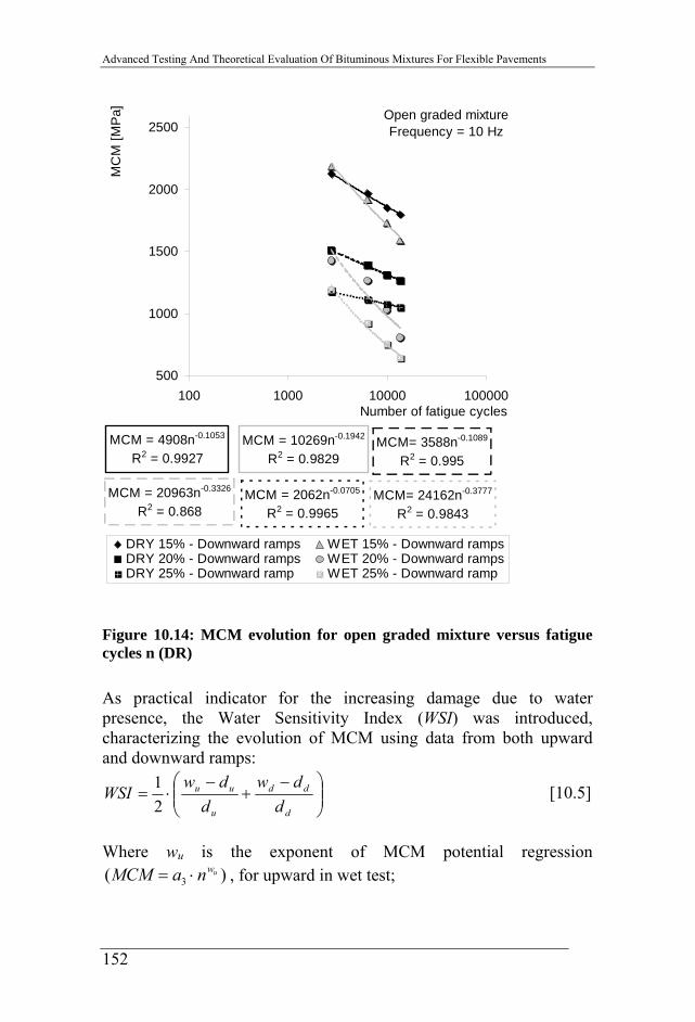
Figure 10.14: MCM evolution for open graded mixture versus fatigue cycles n (DR).................................................................................... 152
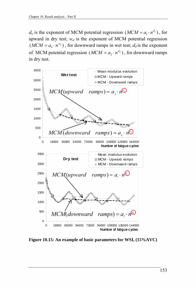
Figure 10.15: An example of basic parameters for WSI, (15%AVC).......................................................................................................... 153
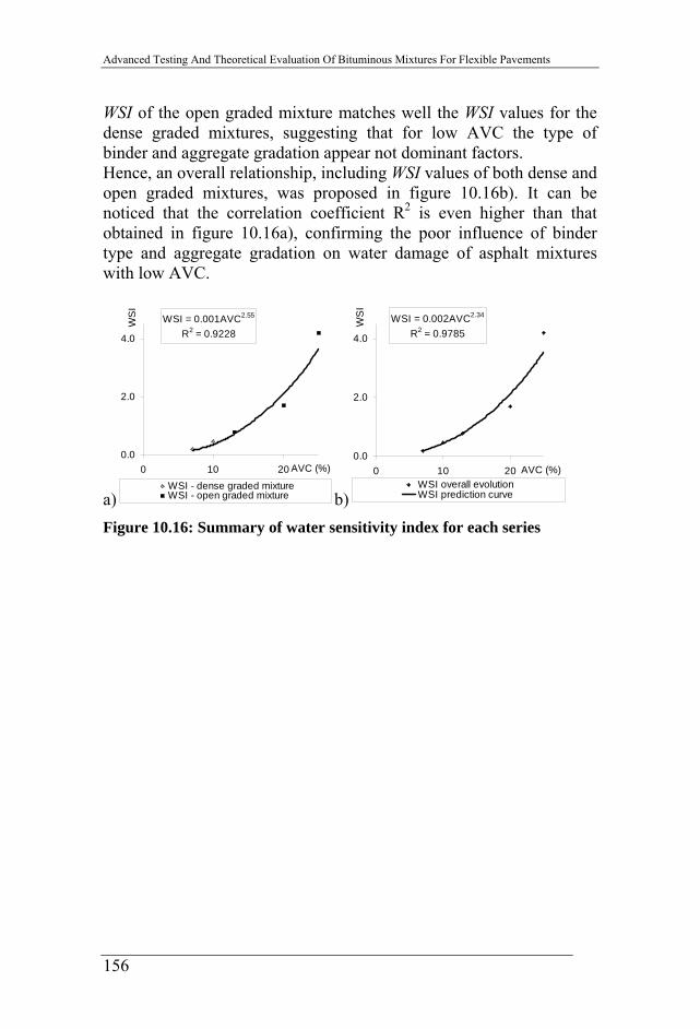
Figure 10.16: Summary of water sensitivity index for each series .. 156
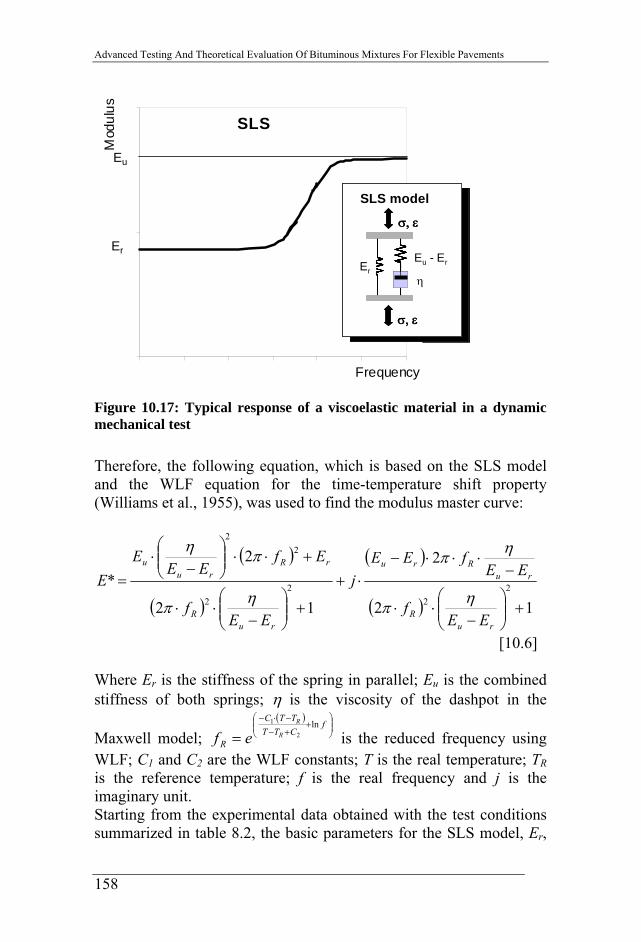
Figure 10.17: Typical response of a viscoelastic material in a dynamic mechanical test ................................................................................. 158
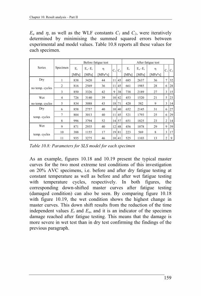
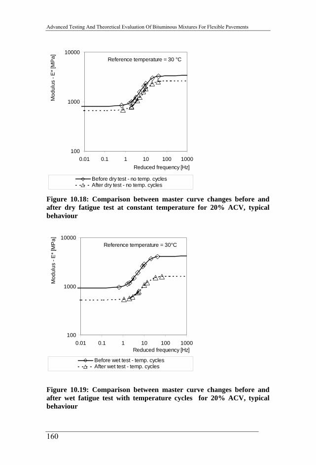
Figure 10.18: Comparison between master curve changes before and after dry fatigue test at constant temperature for 20% ACV, typical behaviour.......................................................................................... 160
Figure 10.19: Comparison between master curve changes before and after wet fatigue test with temperature cycles for 20% ACV, typical behaviour.......................................................................................... 160
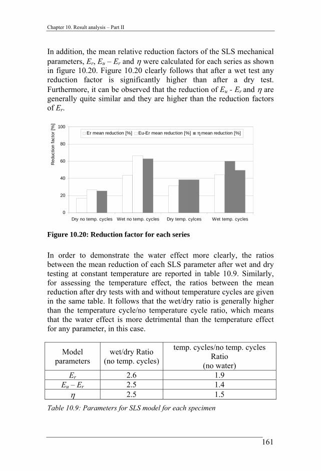
Figure 10.20: Reduction factor for each series ................................ 161
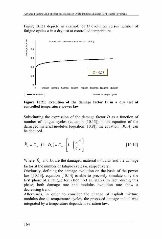
Figure 10.21: Evolution of the damage factor D in a dry test at controlled temperature, power law................................................... 164
10
List of figures
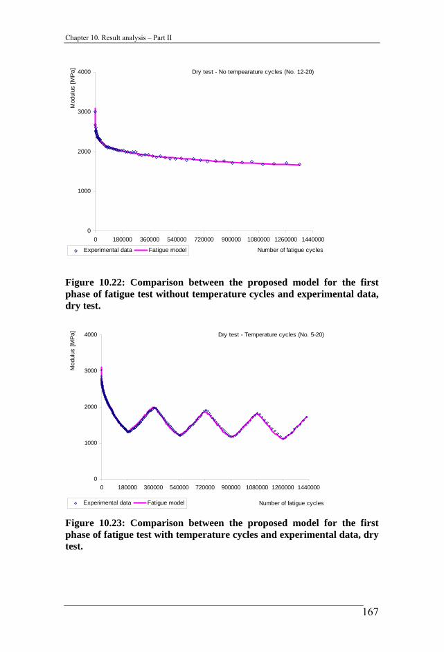
Figure 10.22: Comparison between the proposed model for the first phase of fatigue test without temperature cycles and experimental data, dry test. .................................................................................... 167
Figure 10.23: Comparison between the proposed model for the first phase of fatigue test with temperature cycles and experimental data, dry test. ............................................................................................. 167
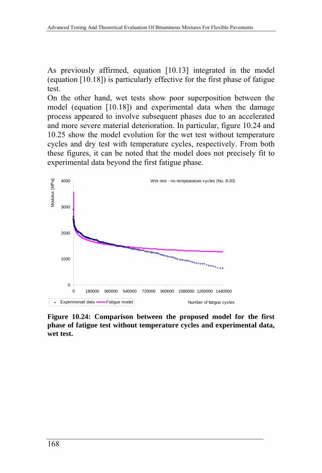
Figure 10.24: Comparison between the proposed model for the first phase of fatigue test without temperature cycles and experimental data, wet test. .................................................................................... 168
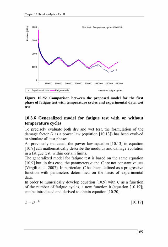
Figure 10.25: Comparison between the proposed model for the first phase of fatigue test with temperature cycles and experimental data, wet test.............................................................................................. 169
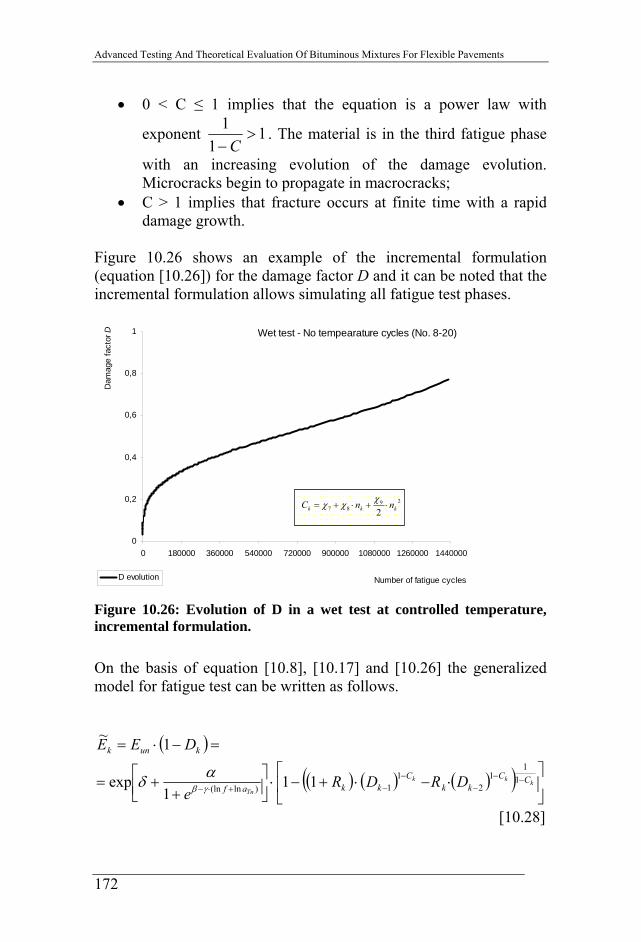
Figure 10.26: Evolution of D in a wet test at controlled temperature, incremental formulation. .................................................................. 172
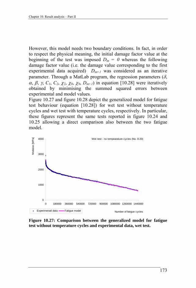
Figure 10.27: Comparison between the generalized model for fatigue test without temperature cycles and experimental data, wet test. .... 173
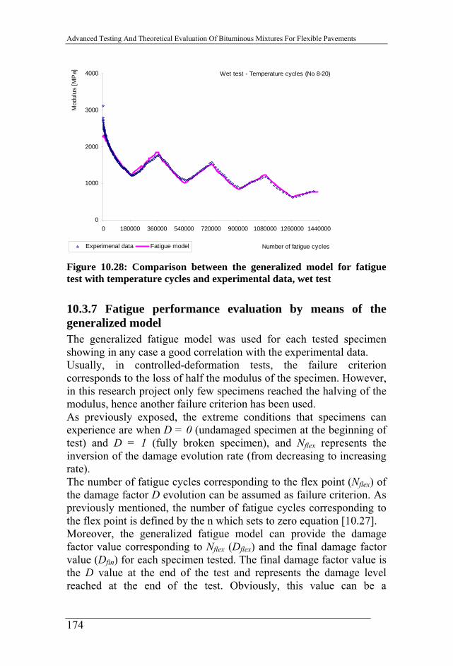
Figure 10.28: Comparison between the generalized model for fatigue test with temperature cycles and experimental data, wet test .......... 174
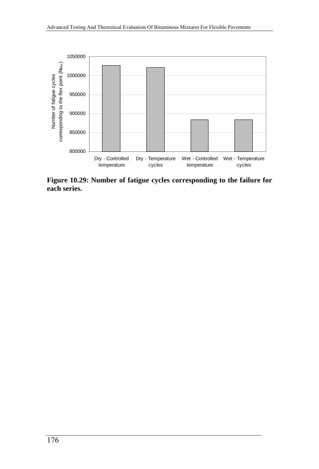
Figure 10.29: Number of fatigue cycles corresponding to the failure for each series................................................................................... 176
11
Advanced Testing And Theoretical Evaluation Of Bituminous Mixtures For Flexible Pavements
12
Abstract
Abstract It is well known that cracking and permanent deformation in asphalt pavements and their related degradation processes can be caused by traffic loading and temperature variations. Moreover, these distresses are often accelerated by water damage mechanisms that generally affect mixture cohesion and/or adhesion between binder and aggregate interface. Nowadays, the increasing traffic, higher axle loads and reduced road maintenance budget, force engineers to seek long lasting materials and reliable testing methods for the design and rehabilitation of asphalt pavements. This thesis focuses on both long-term and durability performance of asphalt pavements. In this context, on one hand the increasing interest in the use of high performance materials, like geosynthetics, drove to determine whether these products act as reinforcement and enable longer service life. On the other hand, a lack of reliable test method for the water sensitivity evaluation of asphalt mixtures led to develop a new experimental method to investigate water and temperature cycle effects in flexible pavements. In order to improve the knowledge on pavement reinforcement use, the Part I of this research project proposes an overall testing protocol analysing shear behaviour, fatigue performance and permanent deformation resistance of geosynthetic-reinforced asphalt pavements. Geosynthetics could not act as a reinforcement product if they are a cause of separation between the layers at the interface. For this reason, this study concerns a better understanding of reinforcement systems behaviour and their effects on mechanical properties of the interface. To this purpose the interlayer direct shear test ASTRA (Ancona Shear Testing Research and Analysis) is used to provide more details regarding the comprehension of the interlayer shear resistance. As previously mentioned, the present work even compares the behaviour of reinforced and unreinforced double-layered prismatic specimens under repeated loading cycles in both controlled deflection and controlled load modes.
13
Advanced Testing And Theoretical Evaluation Of Bituminous Mixtures For Flexible Pavements
Note that in controlled load mode, a theoretical model has been proposed to simulate the permanent deformation evolution curve and the number of loading cycles corresponding to the flex point of the permanent deformation evolution curve was selected as failure criterion. On the other hand, pavement durability may be improved not only by using high performance materials but also by selecting adequate combinations of materials to resist against repeated loading and to mitigate the effects of environmental factors such as water and temperature cycles. For this reason, the Part II of this thesis regards the development of a versatile test method which simultaneously couples both dynamic loading and environmental factors. Tests were carried out on differently compacted specimens with three different approaches: traditional (Indirect Tensile Test), empirical (Cantabro) and innovative (Coaxial Shear Test). In particular, the Coaxial Shear Test (CAST), designed at EMPA since 1980s, is used to determine the evolution of mechanical properties under repeated loading cycles and, in the last years, also combining water action and temperature cycles. Preliminary findings led to concentrate on developing of an effective performance related procedure to characterize water sensitivity of asphalt mixtures with respect to fatigue performance with CAST. In this sense, an elasticity-based damage model has been applied to determine the damage evolution in fatigue test with and without temperature cycles. By evaluating the damage factor evolution the influence of water and temperature cycles on the damage process can be highlighted.
14
Sommario
Sommario Nei paesi industrializzati il deterioramento delle pavimentazioni stradali flessibili, dovuto soprattutto a fenomeni di fessurazione da fatica o di ormaiamento, costituisce un problema sempre più rilevante. Inoltre tali dissesti sono spesso accelerati dall’azione dell’acqua che generalmente indebolisce le proprietà coesive del mastice e di adesione tra bitume e aggregati. Per tali motivi l’interesse nel campo della ricerca stradale si è sempre più focalizzato sullo studio di materiali ad alte prestazioni e sulla messa a punto di protocolli di prova evoluti per la progettazione delle miscele bituminose. In tale ambito, la tesi di dottorato è incentrata sia su un’analisi prestazionale di materiali innovativi di rinforzo per pavimentazioni flessibili quali i geosintetici, sia sul problema generale della durabilità di miscele bituminose. Di conseguenza sono stati considerati anche quei fenomeni di danno apportati non solo dal ripersi ciclico dei carichi, ma anche dall’azione di fattori ambientali quali l’azione dell’acqua e dei cicli termici. Da notare che, anche se entrambi gli argomenti trattati si riconducono al problema comune della “durata” di una sovrastruttura stradale, la presente tesi si struttura in due sezioni distinte. In particolare, nella prima (Part I) si sviluppa un completo protocollo di prova per la verifica degli eventuali benefici apportati dall’uso di geosintetici di rinforzo nelle pavimentazioni flesibili, mentre nella seconda (Part II) si propone una affidabile procedura di prova per la determinazione della sensibilità all’acqua di miscele bituminose. Sulla base di un ampio studio bibliografico si può dedurre che i geosintetici, se non adeguatamente posati in opera, potrebbero non agire come prodotti di rinforzo ma rappresentare un elemento di separazione tra gli strati pregiudicando così l’intera portanza della sovrastruttura. Per questa ragione lo studio inizialmente indaga il comportamento dei sistemi di rinforzo ed il loro effetto sulle proprietà meccaniche all’interstrato tramite la prova di taglio diretto ASTRA (Ancona Shear Testing and Research and Analysis). Successivamente, dopo aver
15
Advanced Testing And Theoretical Evaluation Of Bituminous Mixtures For Flexible Pavements
esaurientemente compreso l’effettiva influenza dei geosintetici nei pacchetti legati, nella seconda parte si paragona il comportamento di sistemi bistrato, rinforzati e non, sottoposti all’azione ciclica in modalità di carico o di deformazione imposta. D’altra parte, la durabilità di una pavimentazione può essere migliorata non solo con l’impiego di materiali ad elevate prestazioni ma anche con una accurata selezione e combinazione dei materiali, al fine di offrire comunque maggiori resistenze contro i carichi ripetuti e mitigare gli effetti dovuti a fattori ambientali quali azione dell’acqua e dei cicli di temperatura. A tale scopo la seconda sezione (Part II) di questa tesi si concentra sullo sviluppo di un metodo di prova versatile che simultaneamente accoppia carichi dinamici e fattori ambientali. Inizialmente lo studio si è basato sul paragone di varie metodologie di prova condotte su provini con diversi livelli di compattazione. In particolare tre approcci distinti sono stati messi a confronto: uno tradizionale (prova a trazione indiretta), uno empirico (prova Cantabro) e uno innovativo (Coaxial Shear Test). Il Coaxial Shear Test (CAST) è un prototipo progettato e realizzato nei laboratori federali svizzeri EMPA sin dagli anni ’80. Negli ultimi anni l’apparecchiatura è stata ulteriormente sviluppata per determinare l’evoluzione delle proprietà meccaniche di miscele bituminose non solo sotto il ripetersi ciclico dei carichi, ma combinando azione dell’acqua e dei cicli di temperatura. I primi risultati ottenuti hanno da subito indirizzato lo studio nella ricerca di una metodologia basata su prove dinamiche ancora più affidabile per la caratterizzazione della sensibilità all’acqua di miscele bituminose. In conclusione un modello è stato appositamente ideato e applicato per la valutazione del processo di danno in prove di fatica con e senza cicli di temperatura. Tale modello permette la valutazione del processo di danno e la determinazione dell’influenza dell’acqua e dei cicli di temperatura sulle proprietà meccaniche della miscela bituminosa studiata.
16
Acknowledgments
Acknowledgments I am indebted to Prof. F. A. Santagata for giving me the opportunity to conduct this research project and to cooperate with the Swiss Federal Laboratories for Materials Testing and Research (EMPA). I would like to express my sincere gratitude to all my supervisors, Prof. M. Bocci, Prof. F. Canestrari and Prof. A. Virgili for their availability and suggestions through these years of study. I wish to express my special thanks to Dr. M. N. Partl for his precious comments and suggestions. It has been an honour for me to have the opportunity to cooperate with him and his highly qualified staff. When working with EMPA, I also had the opportunity to meet the Imboden family. I greatly appreciate their kindness and hospitality. I would also like to thank all my fellow students Dr. G. Ferrotti, Dr. F. Cardone, Dr. E. Pasquini, Dr. V. Pannunzio and Dr. S. Tassetti for their valuable technical support and friendship (Gilda…you are first because you are the most important…honestly?...the oldest!!! Now I have a PhD but I still like joking…). I would like to acknowledge help I received from the staff of Università Politecnica delle Marche and in particular P. Priori, G. Galli and S. Mercuri. My deepest thanks go to my family for their understanding and unlimited patience.
17
Advanced Testing And Theoretical Evaluation Of Bituminous Mixtures For Flexible Pavements
18
Chapter 1: Introduction
Introduction Considering the growth of traffic volume, the deterioration of asphalt pavements is an increasing problematic issue. Nowadays, the most efforts of engineers and researchers deal with the use of high performance materials to extend the pavement service life and design and testing methods based on dynamic mechanical material properties including environmental factors to improve performance prediction and selection of materials. To these purposes this thesis consists of two main sections: the first section deals with an overall testing protocol for bi-layered reinforced asphalt systems and, the second section concerns an effective testing method to evaluate environmental factor effects on dynamic mechanical properties of asphalt mixtures. In pavement design, researchers are trying to improve the mechanical properties and service life of asphalt pavements using geosynthetics. Reinforcements could have several advantages: economic, environmental, technical and functional (Kennepohl et al. 1985). The first application of geosynthetics was in unbound layers to prevent permanent deformation, to improve bearing capacity and to filter and/or separate functions. Currently, considering the growth in traffic volume, engineers have introduced geosynthetics even in asphalt layers in order to reach higher road pavement performance (Austin & Gilchrist, 1996, Brown, 2006). Since 1950’s geosynthetics were used in road construction for providing tensile reinforcement. First attempts showed installation difficulties to lay geosynthetics implying a no correct working of the reinforcement system. Nowadays, more advanced technologies and materials seem to allow the expected improvement. The use of reinforcement systems within bound layers is mainly addressed to prevent or to delay reflective cracking (Brown et al. 2001, Cantabiano & Bruton 1991, Gillespie & Roffe, 2002, Elseifi & Al Qadi, 2003, Montestruque et al., 2004, Sobhan et al., 2004), rutting (Komatsu et al., 1998) and fatigue failure (Brown et al., 1985).
19
Advanced Testing And Theoretical Evaluation Of Bituminous Mixtures For Flexible Pavements
However, the correct action of a reinforcing system at the interface should satisfy both mechanical needs of multilayered road pavements in terms of bending and shear performance (Brown et al., 2001, Caltabiano and Brunton, 1991). In particular, the first section of this thesis studies the effects of different interlayer materials on mechanical properties of bi-layered bituminous systems. According to numerous theoretical and experimental studies the interaction between layers at interface influences the bearing capacity, the load distribution and therefore the performance of the asphalt pavements. For this reason, the experimental program has been based on shear test with Ancona Shear Testing Research and Analysis (ASTRA) and four point bending test. In particular, four types of geosynthetics at the interface were used in order to investigate the influence of the reinforcement properties (stiffness, geometry, mesh size, coating, etc.) on the interlayer shear strength and the resistance against repeated loading cycles. ASTRA considers the effects of various test parameters, such as temperature and normal stress, and distinguishes without ambiguity the performance of different interlayer configurations. In four point bending test, several parameters can be selected in order to identify a failure criterion and, then, to evaluate mechanical performance of asphalt mixtures. In this case, test results were elaborated considering the following approaches:
• dissipated energy for controlled deflection mode; • number of cycles of applied load to failure for controlled load
mode. Moreover, in controlled load mode, an original permanent deformation evolution model has been used to simulate the experimental data and to precisely determine the flex point of the permanent deformation curve. The number of loading cycles corresponding to the flex point of the permanent deformation curve has been assumed as failure criterion. In fact, considering that in this kind of test, two main phenomena may be distinguished, i.e., hardening and damage, the flex point of the permanent deformation evolution curve may represent the separation or balance point between hardening phase and damage process.
20
Chapter 1: Introduction
The second section, related to water sensitivity of asphalt mixture, has been developed in cooperation with EMPA (Swiss Federal Laboratories for Materials Testing and Research). Two mechanisms are related to water damage: cohesion failure and adhesive failure (R. G. Hicks et al., 2003). A loss of cohesion causes an overall weakening such as a reduction of strength and stiffness, based on the emulsification of water in the asphalt binder film, thus generating failure within the asphalt binder film coat of the aggregate (Fromm, 1974) and reducing resistance against stresses and strains. Adhesion failure, on the other hand, typically results in debonding of aggregate and binder, implying progressive loss of material and ravelling (Kandhal et al., 1989, Kandhal and Rickards, 2001). Since, it is difficult to distinguish between cohesion and adhesion failure modes, one can assume that, generally, deterioration of asphalt pavements in presence of water is caused by both failure modes in a coupled way. Numerous research projects have been conducted to understand and predict moisture damage in asphalt mixtures and remarkable progress has been made up to now (Al-Swailmi and Terrel, 1992, Terrel and Al-Swailmi, 1994, Nguyen et al., 1996, Epps et al., 2000, West et al., 2004, Kim and Coree, 2005, Airey et al., 2003, Kim and Coree, 2006). As a result, different test methods and procedures have been developed. In particular, they may be generally classified into two main categories: tests performed on loose mixtures and tests carried out on compacted mixtures (Kiggundu and Roberts, 1988, Brown et al. 2001, Airey and Choi, 2002, Solaimanian et al., 2003). Tests on loose asphalt mixtures focus on moisture related adhesion and cohesion failure for subjective evaluation and assessment of stripping potential. Asphalt mixtures are usually immersed in water for a specific time at constant temperature and visually inspected in search of “stripped” or uncoated aggregates (Kennedy and Ping, 1991, Dunning et al., 1993, Aschenbrener et al., 1995). Tests on compacted asphalt mixtures may be further categorized into both rutting tests on asphalt pavement slabs evaluating the development of permanent deformation under repeated wheel loading in presence of water (Smit et al., 2002, Raab et al., 2005, Solaimanian et al., 2006) and static or cyclic loading tests where the reduction of selected mechanical properties of compacted specimens or cores during or after immersion in water are determined (Al-Swailmi and Terrel, 1992, Aschenbrener et al., 1995, Kim and Coree, 2006, Solaimanian et al., 2006).
21
Advanced Testing And Theoretical Evaluation Of Bituminous Mixtures For Flexible Pavements
However, because of many different influence factors and complexity of effects, moisture damage phenomena and mechanisms are still far of being fully understood and considerable, research is still needed. So far, none of the laboratory tests has provided a conclusive method to characterize the effects of moisture on mechanical properties of asphalt mixtures in a satisfactory way and the search for improved performance-related test methods is still ongoing worldwide. Therefore the subject of the second section of this thesis is to propose a new method to characterize water sensitivity of asphalt mixtures with respect to fatigue performance. It uses the CoAxial Shear Test CAST (Gubler et al., 2004, Gubler et al., 2005, Partl 2007), which is a performance related laboratory test procedure for laboratory produced specimens and cores with lateral confinement that allows combining both climatic and traffic-like cyclic loading. Moreover, an elasticity-based damage model has been applied to determine the damage evolution in fatigue test with and without temperature cycles (Virgili et al., 2007).
22
Part I
Geosynthetics in bound layers
23
Advanced Testing And Theoretical Evaluation Of Bituminous Mixtures For Flexible Pavements
24
Chapter 1. Literature review – Part I
1. Literature review – Part I Numerous detrimental factors affect the service life of asphalt pavement in terms of mechanical and functional performance. These factors, such as environmental conditions, subgrade conditions, traffic loading and ageing, prematurely addressed to rehabilitation or maintenance of asphalt pavements if not adequately took into account during design and construction phases. Moreover, pavement maintenance treatments can be ineffective if they do not act against the real detrimental causes. Nowadays, geosynthetics can be used for both long-term road during initial construction and cost-effective maintenance (Brown 2006). The five main functions of geosynthetics in road construction are:
• Separation and filtration; • Stabilization; • Reinforcement and Stress absorption.
The separation function is primary characteristic of geotextiles in road construction. In this case, the geosynthetics acts as a separator between the soft subgrade and the aggregates avoiding the intrusion of cohesive soil in upper layers. In this way the initial thickness and mechanical characteristics of road layers are preserved. In addition, the separation function has to be combined with the filtration function to allow water drainage and to avoid interstitial pressure which can cause differential settlements. The stiffness properties of geosynthetics are essential for the stabilization function. A considerable reduction of aggregates or an increasing of bearing capacity is possible by the use of a geosynthetics which implies the membrane action, a lateral restrain and confinement of aggregates. The reinforcement function in a continuum body is obtained by insertion of reinforcing materials able to improve mechanical properties of the continuum body. The main reinforcement mechanisms are:
25
Advanced Testing And Theoretical Evaluation Of Bituminous Mixtures For Flexible Pavements
• Confinement of materials and enhancement of the load
distribution capacity; • Enhancement of ductility at low temperatures; • Reduction of tensile stress.
To note that the reinforcement behaviour in bound layers differs from the reinforcement behaviour in unbound layers. This thesis focuses on the use of geosynthetics in bound layers, hence, the following paragraphs deal with this specific issue. The reinforcement function in asphalt layers can be further summarized in:
• Extension of fatigue life or reduction of thickness layers (Brown et al., 1985, Brown et al., 2001);
• Elimination or limitation of reflective cracking (Cantabiano and Bruton 1991, Brown et al. 2001, Gillespie and Roffe, 2002, Elseifi & Al Qadi 2003, Mostafa and Al-Qadi, 2003, Montestruque et al., 2004, Sobhan et al., 2004);
• Reduction of rutting (Brown et al., 1985, Komatsu et al., 1998).
Fatigue failure occurs when a body is subjected to repeated loading cycles. The tyre weight causes a local bending of the asphalt pavement and tensile stresses are generated at the bottom of bound layers. Even though the induced-tensile stresses are lower than the failure strength of materials, the repeated action of these stresses reduces the material resistance and causes microcracking and then their propagation up to fracture. In this case, stiff geosynthetics contribute to absorb tensile stresses enabling longer service life. The reflective cracking failure typically occurs in asphalt overlay by propagation of existing cracks or discontinuities in old asphalt pavement. Repeated loading and thermal cycles generate tensile stresses on the tip of predefined cracks leading to premature failure. Once reflection cracking propagates the overlay becomes more susceptible to adverse environmental factors such as water infiltration and premature oxidation. In this case, geosynthetics give a contribution to resist against these tensile stresses at the interface and delay the rising of cracks. It is worth note that the correct action of a reinforcing system at the interface should satisfy both mechanical
26
Chapter 1. Literature review – Part I
needs of multilayered road pavements in terms of bending and their shear performance (Brown et al., 2001, Caltabiano and Brunton, 1991). Rutting is due to the accumulation of permanent deformations or densification under loading cycles and high temperatures and appears as longitudinal depressions in the wheel paths. Rutting reduces the comfort of the pavement and, by affecting vehicle handling characteristics, creates serious hazards for highway users. In this case, the geosynthetic have to avoid plastic deformation and distribute shear loading. The most important characteristic of the geosynthetic is the geometry and the size of meshes and ribs which have to allow mechanical interlocking between the geosynthetic and the surrounding material. Currently, two different approaches are used to study the mechanical properties of asphalt pavements: empirical approach and theoretical approach. The empirical approach is based on physical principles, experiences and relative standard testing methods. This approach generally provides easy response related to the material behaviour but it can be rather approximate when applied to complex cases. The theoretical approach, such as finite element method or finite difference method, is based on numerical modelling which can deal with complex situations and offer different solutions. This approach can take into account the unhomogeneity and the non linear behaviour of materials. However, the reliability of this approach depends on the schematization of materials and on the constitutive law used. Both approaches have been used to understand the behaviour and the effects of geosynthetics in asphalt layers. The attempt of providing tensile reinforcement for asphalt pavements goes back to 1950’s. At the beginning all attempts experienced installation difficulties in laying the mesh flat but afterwards, with new technology, there were evidences of possible benefits related to the use of geosynthetics in road construction. However, the use of geosynthetics in asphalt layers is still considered a high-risk solution due to a lack of detailed design procedure.
1.1 Location of geosynthetics in asphalt layer Reinforcement can be placed in different alternative locations in a road structure. Investigations carried out at the Nottingham University established that the use of geosynthetics in asphalt layers could
27
Advanced Testing And Theoretical Evaluation Of Bituminous Mixtures For Flexible Pavements
significantly improve the asphalt pavement performance (Brown et al., 2001). These studies also showed that the location of the grid within the asphalt layer is an essential issue as shown figure 1.1.
Figure 1.1: Pavement cross-sections (Brown et al., 2001).
Figure 1.1 depicts three cross-sections of an 80 mm asphalt mixture layer which were constructed over a low stiffness granular base and subgrade and were subjected to the same wheel load of 9 kN for 200000 repetitions at 20°C. The top cross-section is the unreinforced layer, the middle cross-section has a grid located at the mid-deph of the layer while the lower cross-section has a grid located at the bottom of the layer. The unreinforced section has failed by cracking and significant rut depth involves both asphalt layer and supporting layers. The section with grid at mid-depth (where the maximum permanent shear strains are generally located) shows cracking but the asphalt layer thickness has been maintained. In fact, permanent deformation has been limited by grid and the rutting is caused by a failure of the supporting layers. The section with grid at the bottom (where the maximum tensile strains are located) does not show cracking and preserves the structural integrity. The small amount of rutting is shown in the asphalt layer while the permanent deformation is the lowest in the supporting layers (Brown et al., 2001). Other authors (Sobhan at al., 2004) evaluated the effects of placement location of the geogrid on propagation of reflection cracks. Four types of double-layered specimens were prepared: unreinforced specimens
28
Chapter 1. Literature review – Part I
(as control specimens), specimens with geogrid attached at the bottom, specimens with geogrid embedded at the bottom, specimens with geogrid placed in the middle of asphalt beam. After demoulding , two plywood pieces were attached at the bottom of the specimen with a gap of 1 cm and placed on the rubber foundation for testing. Both reinforced and unreinforced specimens were tested under static and cyclic tests showing greater resistance to reflective cracking when compared with unreinforced specimens. Moreover, as shown in figure 1.2, geogrid embedded at the mid-height was more effective compared with greogrid embedded at the bottom of the asphalt layer.
Figure 1.2: Behaviour of reinforced and unreinforced beam under repeated loading (Sobhan at al., 2004).
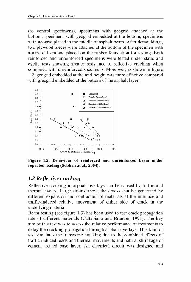
1.2 Reflective cracking Reflective cracking in asphalt overlays can be caused by traffic and thermal cycles. Large strains above the cracks can be generated by different expansion and contraction of materials at the interface and traffic-induced relative movement of either side of crack in the underlying material. Beam testing (see figure 1.3) has been used to test crack propagation rate of different materials (Caltabiano and Brunton, 1991). The key aim of this test was to assess the relative performance of treatments to delay the cracking propagation through asphalt overlays. This kind of test simulates the transverse cracking due to the combined effects of traffic induced loads and thermal movements and natural shrinkage of cement treated base layer. An electrical circuit was designed and
29
Advanced Testing And Theoretical Evaluation Of Bituminous Mixtures For Flexible Pavements
attached to the face of the beam. While the crack propagated up the beam face the electrical strips broke allowing the monitoring of crack growth.
Figure 1.3: Beam testing equipment (Brown et al., 2001).
Each series of specimens reinforced with the respective treatment was compared with the control series of unreinforced specimens. Treatments were compared through a factor on life related to the control series life. By applying a vertical traffic load of 555 kPa the factors in life were:
• 2.5 for polymer modified binder • 5.0 for geotextile interlayer • 10.0 for geogrid interlayer
By increasing the vertical traffic load up to 810 kPa the tensile properties of interlayer treatments appeared to improve their relative life as follows:
• 2.5 for polymer modified binder • 15.0 for geotextile interlayer • 31.0 for geogrid interlayer
However, the installation techniques have proved essential to the success of interlayer treatments in field. Other authors (Austin and Gilchrist, 1996) used a series of slabs trafficked by a moving wheel load over a rubber support. Slabs (60 mm thick layer of asphalt mixture and 20 mm thick sandsheet) were tack coated over a plywood support with a 100 mm gap. Interlayer treatments were applied between the asphalt mixture and sandsheet
30
Chapter 1. Literature review – Part I
layer and compared with the control series. The crack propagation thorough the slab section was caused by repeated opening and closing of the gap between the plywood supports under wheel loading which generated a cycle maximum tensile strain. By comparing the failure number of wheel passes, it can be noted that slabs reinforced with geogrid resisted 3.94 times more than slabs unreinforced while slabs reinforced with composite resisted 7.58 times more than slabs unreinforced. Furthermore, the use of fibre-reinforced membrane or interlayer stress-absorbing composite to inhibit reflective cracking was evaluated by other authors (Gillespie and Roffe, 2002, Dempsey, 2002). Laboratory research and site monitoring indicated that the use of both products (i.e. fibre-reinforced membrane and interlayer stress-absorbing composite) significantly reduces the reflective cracking.
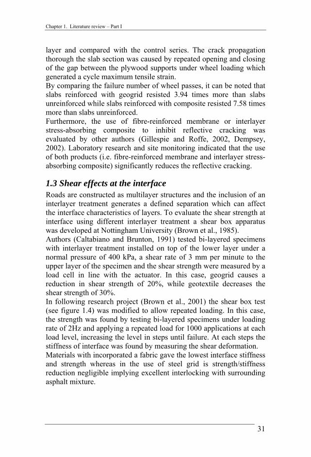
1.3 Shear effects at the interface Roads are constructed as multilayer structures and the inclusion of an interlayer treatment generates a defined separation which can affect the interface characteristics of layers. To evaluate the shear strength at interface using different interlayer treatment a shear box apparatus was developed at Nottingham University (Brown et al., 1985). Authors (Caltabiano and Brunton, 1991) tested bi-layered specimens with interlayer treatment installed on top of the lower layer under a normal pressure of 400 kPa, a shear rate of 3 mm per minute to the upper layer of the specimen and the shear strength were measured by a load cell in line with the actuator. In this case, geogrid causes a reduction in shear strength of 20%, while geotextile decreases the shear strength of 30%. In following research project (Brown et al., 2001) the shear box test (see figure 1.4) was modified to allow repeated loading. In this case, the strength was found by testing bi-layered specimens under loading rate of 2Hz and applying a repeated load for 1000 applications at each load level, increasing the level in steps until failure. At each steps the stiffness of interface was found by measuring the shear deformation. Materials with incorporated a fabric gave the lowest interface stiffness and strength whereas in the use of steel grid is strength/stiffness reduction negligible implying excellent interlocking with surrounding asphalt mixture.
31
Advanced Testing And Theoretical Evaluation Of Bituminous Mixtures For Flexible Pavements
Figure 1.4: Repeated load shear test for interfaces (Brown et al., 2001).
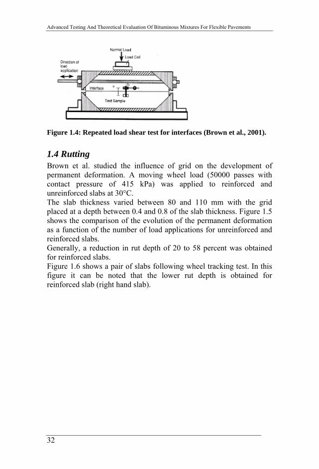
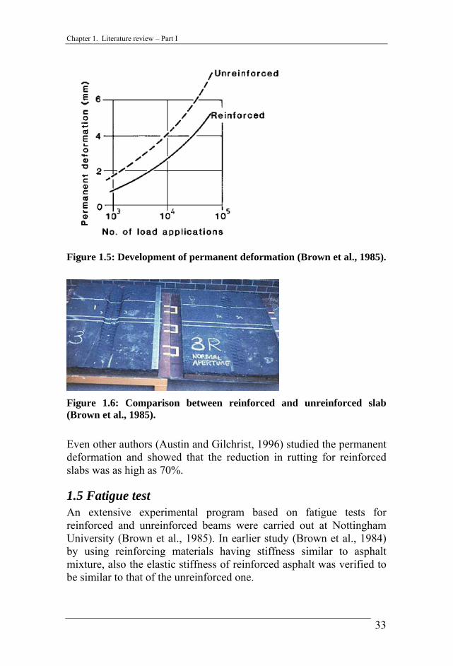
1.4 Rutting Brown et al. studied the influence of grid on the development of permanent deformation. A moving wheel load (50000 passes with contact pressure of 415 kPa) was applied to reinforced and unreinforced slabs at 30°C. The slab thickness varied between 80 and 110 mm with the grid placed at a depth between 0.4 and 0.8 of the slab thickness. Figure 1.5 shows the comparison of the evolution of the permanent deformation as a function of the number of load applications for unreinforced and reinforced slabs. Generally, a reduction in rut depth of 20 to 58 percent was obtained for reinforced slabs. Figure 1.6 shows a pair of slabs following wheel tracking test. In this figure it can be noted that the lower rut depth is obtained for reinforced slab (right hand slab).
32
Chapter 1. Literature review – Part I
Figure 1.5: Development of permanent deformation (Brown et al., 1985).
Figure 1.6: Comparison between reinforced and unreinforced slab (Brown et al., 1985).
Even other authors (Austin and Gilchrist, 1996) studied the permanent deformation and showed that the reduction in rutting for reinforced slabs was as high as 70%.
1.5 Fatigue test An extensive experimental program based on fatigue tests for reinforced and unreinforced beams were carried out at Nottingham University (Brown et al., 1985). In earlier study (Brown et al., 1984) by using reinforcing materials having stiffness similar to asphalt mixture, also the elastic stiffness of reinforced asphalt was verified to be similar to that of the unreinforced one.
33
Advanced Testing And Theoretical Evaluation Of Bituminous Mixtures For Flexible Pavements
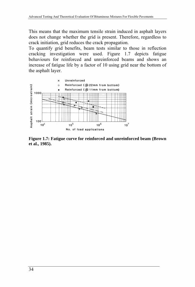
This means that the maximum tensile strain induced in asphalt layers does not change whether the grid is present. Therefore, regardless to crack initiation, grid reduces the crack propagation. To quantify grid benefits, beam tests similar to those in reflection cracking investigation were used. Figure 1.7 depicts fatigue behaviours for reinforced and unreinforced beams and shows an increase of fatigue life by a factor of 10 using grid near the bottom of the asphalt layer.
Figure 1.7: Fatigue curve for reinforced and unreinforced beam (Brown et al., 1985).
34
Chapter 2. Materials – Part I
2. Materials – Part I
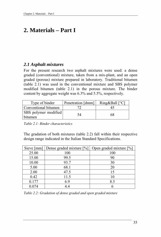
2.1 Asphalt mixtures For the present research two asphalt mixtures were used: a dense graded (conventional) mixture, taken from a mix-plant, and an open graded (porous) mixture prepared in laboratory. Traditional bitumen (table 2.1) was used in the conventional mixture and SBS polymer modified bitumen (table 2.1) in the porous mixture. The binder content by aggregate weight was 6.3% and 5.5%, respectively.
Type of binder Penetration [dmm] Ring&Ball [°C] Conventional bitumen 72 45 SBS polymer modified bitumen 54 68
Table 2.1: Binder characteristics
The gradation of both mixtures (table 2.2) fall within their respective design range indicated in the Italian Standard Specifications. Sieve [mm] Dense graded mixture [%] Open graded mixture [%]
Table 2.2: Gradation of dense graded and open graded mixture
35
Advanced Testing And Theoretical Evaluation Of Bituminous Mixtures For Flexible Pavements
2.2 Reinforcing materials In this study four different reinforcing materials were used in order to investigate their effects on shear resistance at interface and fatigue behaviour.
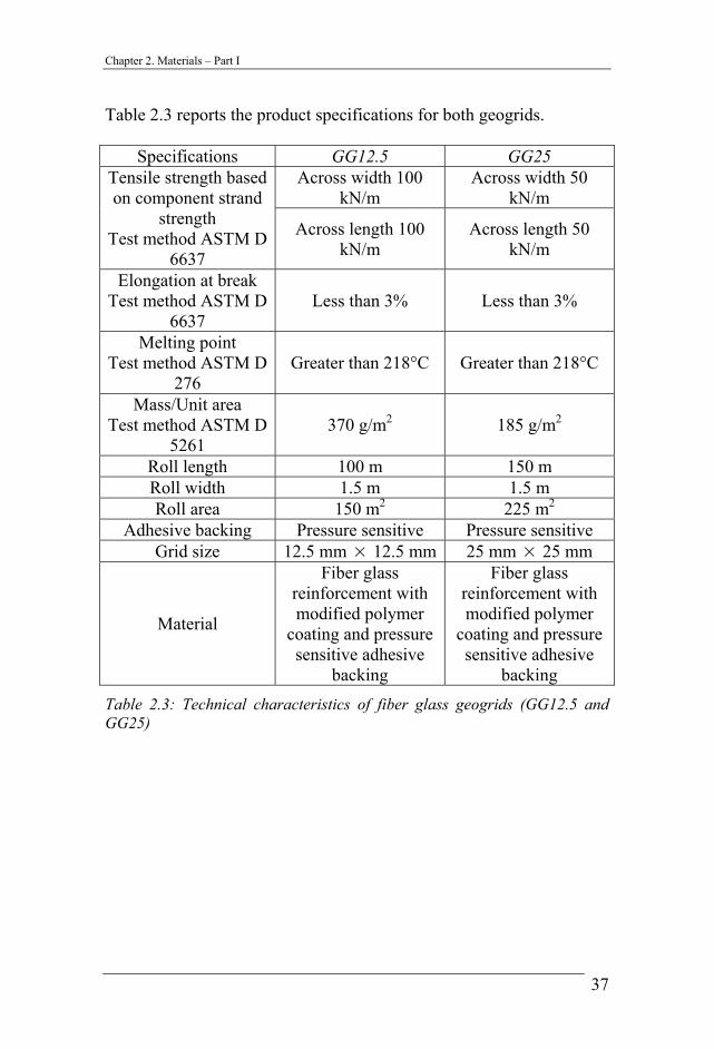
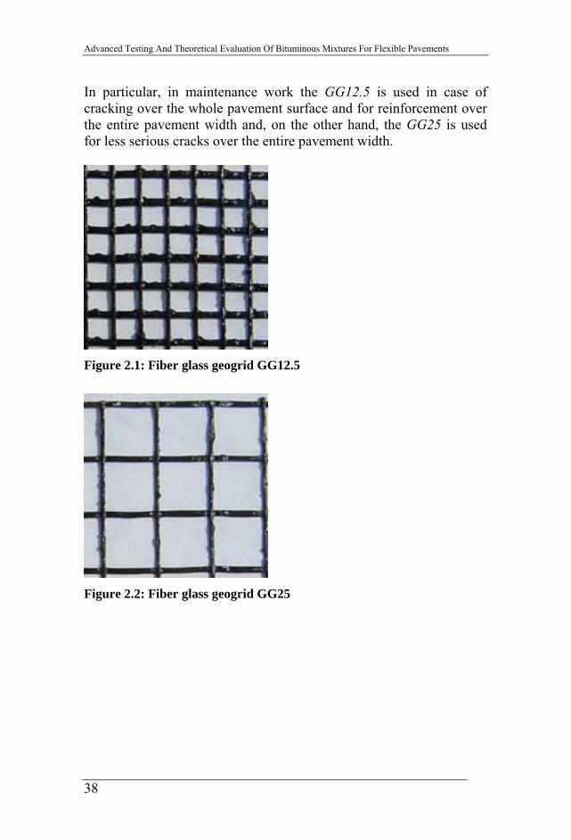
2.2.1 Geogrids A geogrid is defined as a deformed or nondeformed regular grid structure of polymeric material formed by joined intersecting ribs used for reinforcement. To be effective, it must have aperture geometry, rib, and rib junction cross sections sufficient to permit significant mechanical interlock with the material being reinforced and high tensile strength value. Two Glass fiber Geogrid, so-called GG12.5 (figure 2.1) and GG25 (figure 4.2), with modified polymer coating were used. GG12.5 is produced with a mesh size of 12.5×12.5 mm2 and tensile strength of 100 KN/m. GG25 is produced with a mesh size of 25×25 mm2 and tensile strength of 50 KN/m.
36
Chapter 2. Materials – Part I
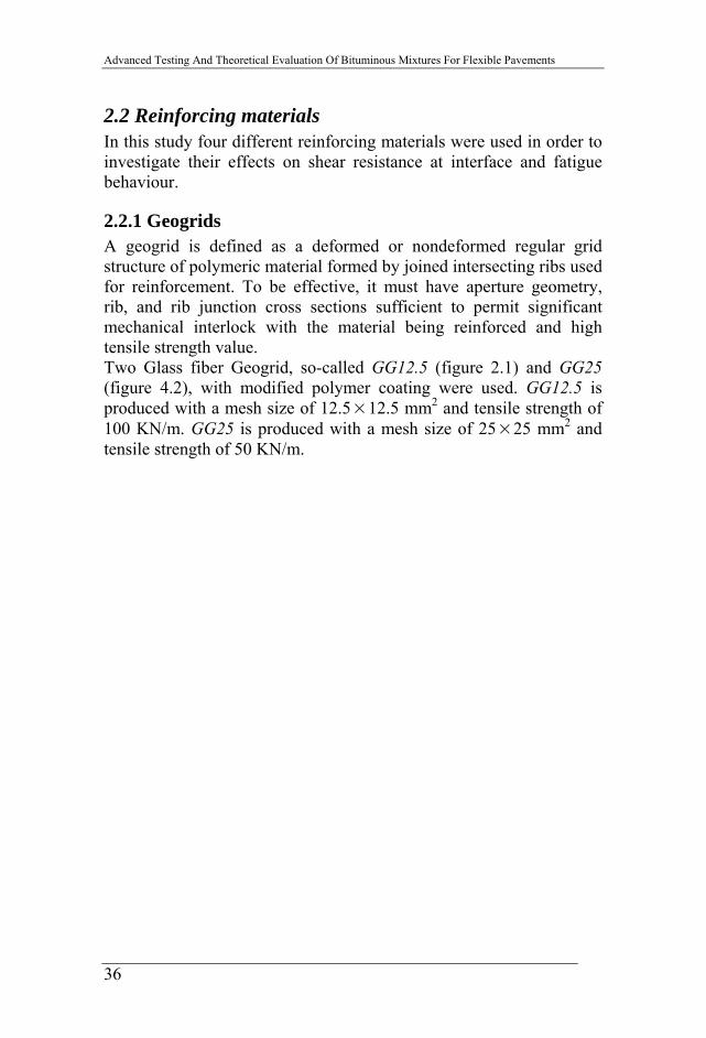
Table 2.3 reports the product specifications for both geogrids.
Specifications GG12.5 GG25 Across width 100
kN/m Across width 50
kN/m Tensile strength based on component strand
strength Test method ASTM D
6637
Across length 100 kN/m
Across length 50 kN/m
Elongation at break Test method ASTM D
6637 Less than 3% Less than 3%
Melting point Test method ASTM D
276 Greater than 218°C Greater than 218°C
Mass/Unit area Test method ASTM D
5261 370 g/m2 185 g/m2
Roll length 100 m 150 m Roll width 1.5 m 1.5 m Roll area 150 m2 225 m2
Adhesive backing Pressure sensitive Pressure sensitive Grid size 12.5 mm × 12.5 mm 25 mm × 25 mm
Material
Fiber glass reinforcement with modified polymer
coating and pressure sensitive adhesive
backing
Fiber glass reinforcement with modified polymer
coating and pressure sensitive adhesive
backing Table 2.3: Technical characteristics of fiber glass geogrids (GG12.5 and GG25)
37
Advanced Testing And Theoretical Evaluation Of Bituminous Mixtures For Flexible Pavements
In particular, in maintenance work the GG12.5 is used in case of cracking over the whole pavement surface and for reinforcement over the entire pavement width and, on the other hand, the GG25 is used for less serious cracks over the entire pavement width.
Figure 2.1: Fiber glass geogrid GG12.5
Figure 2.2: Fiber glass geogrid GG25
38
Chapter 2. Materials – Part I
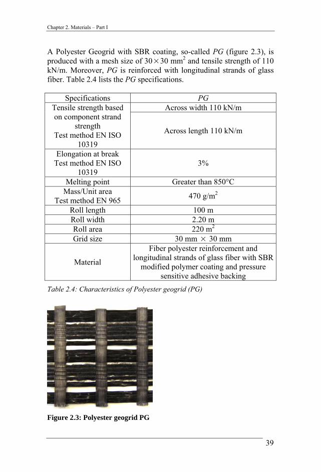
A Polyester Geogrid with SBR coating, so-called PG (figure 2.3), is produced with a mesh size of 30×30 mm2 and tensile strength of 110 kN/m. Moreover, PG is reinforced with longitudinal strands of glass fiber. Table 2.4 lists the PG specifications.
Specifications PG Across width 110 kN/m Tensile strength based
on component strand strength
Test method EN ISO 10319
Across length 110 kN/m
Elongation at break Test method EN ISO
10319 3%
Melting point Greater than 850°C Mass/Unit area
Test method EN 965 470 g/m2
Roll length 100 m Roll width 2.20 m Roll area 220 m2
Grid size 30 mm × 30 mm
Material
Fiber polyester reinforcement and longitudinal strands of glass fiber with SBR
modified polymer coating and pressure sensitive adhesive backing
Table 2.4: Characteristics of Polyester geogrid (PG)
Figure 2.3: Polyester geogrid PG
39
Advanced Testing And Theoretical Evaluation Of Bituminous Mixtures For Flexible Pavements
2.2.2 Emulsion
A cationic bituminous emulsion, with a dosage of 0.3 kg/m2 of residual bitumen, was used to fix the geogrids between the underlay and the overlay in the case of CIC system (Conventional mix/Interlayer/Conventional mix), while for CIP system (Conventional mix/Interlayer/Porous mix) the chosen residual bitumen amount was 1.2 kg/m2. Emulsion properties are shown in table 2.5.
Emulsion type % residual bitumen
Penetration [dmm] Ring&Ball [°C]
Cationic emulsion 69 69 53
Table 2.5: Emulsion characteristics
40
Chapter 2. Materials – Part I
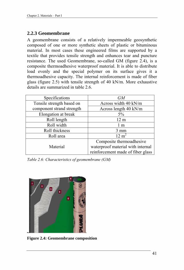
2.2.3 Geomembrane A geomembrane consists of a relatively impermeable geosynthetic composed of one or more synthetic sheets of plastic or bituminous material. In most cases these engineered films are supported by a textile that provides tensile strength and enhances tear and puncture resistance. The used Geomembrane, so-called GM (figure 2.4), is a composite thermoadhesive waterproof material. It is able to distribute load evenly and the special polymer on its surface gives it a thermoadhesive capacity. The internal reinforcement is made of fiber glass (figure 2.5) with tensile strength of 40 kN/m. More exhaustive details are summarized in table 2.6.
Specifications GM Across width 40 kN/m Tensile strength based on
component strand strength Across length 40 kN/m Elongation at break 5%
Roll length 12 m Roll width 1 m
Roll thickness 3 mm Roll area 12 m2
Material Composite thermoadhesive
waterproof material with internal reinforcement made of fiber glass
Table 2.6: Characteristics of geomembrane (GM)
Figure 2.4: Geomembrane composition
41
Advanced Testing And Theoretical Evaluation Of Bituminous Mixtures For Flexible Pavements
Figure 2.5: Internal reinforcement of fiber glass
Generally, in maintenance work this kind of geomembrane is used in case of cracking over the whole pavement surface and for reinforcement over the entire pavement width but also in case of local damage such as transverse and longitudinal cracks and for joints in asphalt and concrete pavements.
42
Chapter 3. Experimental program – Part I
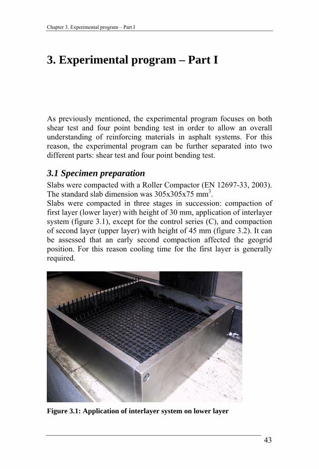
3. Experimental program – Part I As previously mentioned, the experimental program focuses on both shear test and four point bending test in order to allow an overall understanding of reinforcing materials in asphalt systems. For this reason, the experimental program can be further separated into two different parts: shear test and four point bending test.
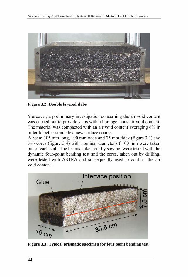
3.1 Specimen preparation Slabs were compacted with a Roller Compactor (EN 12697-33, 2003). The standard slab dimension was 305x305x75 mm3. Slabs were compacted in three stages in succession: compaction of first layer (lower layer) with height of 30 mm, application of interlayer system (figure 3.1), except for the control series (C), and compaction of second layer (upper layer) with height of 45 mm (figure 3.2). It can be assessed that an early second compaction affected the geogrid position. For this reason cooling time for the first layer is generally required.
Figure 3.1: Application of interlayer system on lower layer
43
Advanced Testing And Theoretical Evaluation Of Bituminous Mixtures For Flexible Pavements
Figure 3.2: Double layered slabs
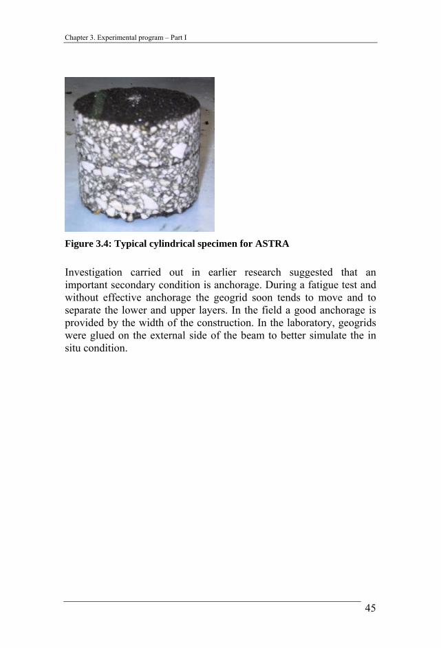
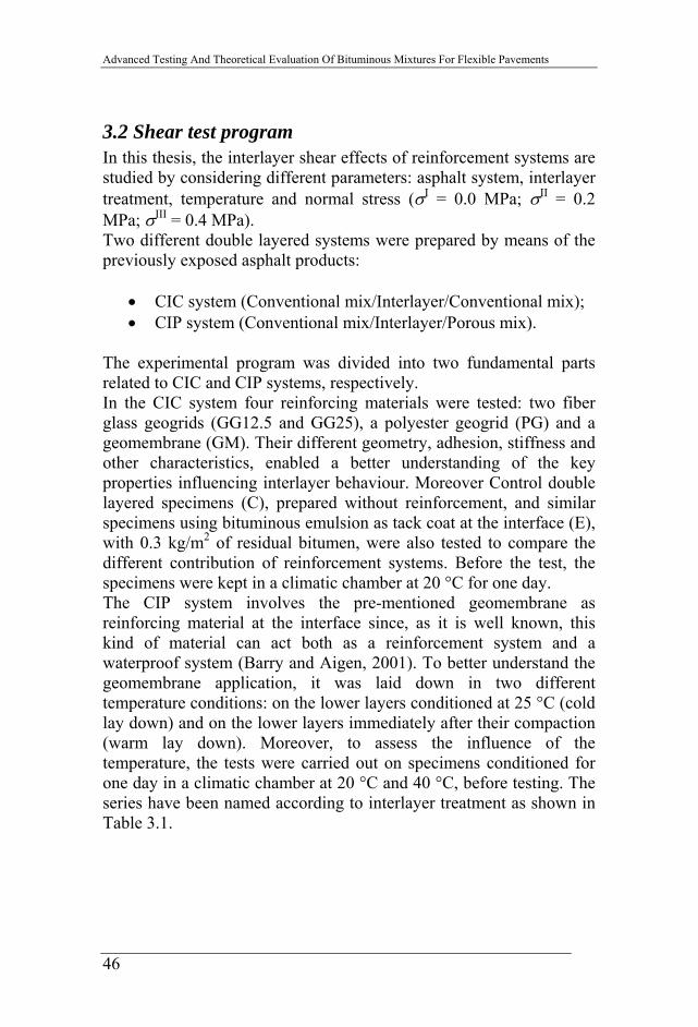
Moreover, a preliminary investigation concerning the air void content was carried out to provide slabs with a homogeneous air void content. The material was compacted with an air void content averaging 6% in order to better simulate a new surface course. A beam 305 mm long, 100 mm wide and 75 mm thick (figure 3.3) and two cores (figure 3.4) with nominal diameter of 100 mm were taken out of each slab. The beams, taken out by sawing, were tested with the dynamic four-point bending test and the cores, taken out by drilling, were tested with ASTRA and subsequently used to confirm the air void content.
10 cm 30.5 cm
7.5
cm
Interface positionGlue
10 cm 30.5 cm
7.5
cm
Interface positionGlue
Figure 3.3: Typical prismatic specimen for four point bending test
44
Chapter 3. Experimental program – Part I
Figure 3.4: Typical cylindrical specimen for ASTRA
Investigation carried out in earlier research suggested that an important secondary condition is anchorage. During a fatigue test and without effective anchorage the geogrid soon tends to move and to separate the lower and upper layers. In the field a good anchorage is provided by the width of the construction. In the laboratory, geogrids were glued on the external side of the beam to better simulate the in situ condition.
45
Advanced Testing And Theoretical Evaluation Of Bituminous Mixtures For Flexible Pavements
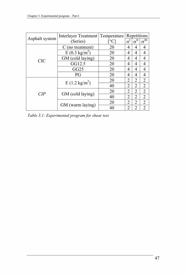
3.2 Shear test program In this thesis, the interlayer shear effects of reinforcement systems are studied by considering different parameters: asphalt system, interlayer treatment, temperature and normal stress (σI = 0.0 MPa; σII = 0.2 MPa; σIII = 0.4 MPa). Two different double layered systems were prepared by means of the previously exposed asphalt products:
• CIC system (Conventional mix/Interlayer/Conventional mix); • CIP system (Conventional mix/Interlayer/Porous mix).
The experimental program was divided into two fundamental parts related to CIC and CIP systems, respectively. In the CIC system four reinforcing materials were tested: two fiber glass geogrids (GG12.5 and GG25), a polyester geogrid (PG) and a geomembrane (GM). Their different geometry, adhesion, stiffness and other characteristics, enabled a better understanding of the key properties influencing interlayer behaviour. Moreover Control double layered specimens (C), prepared without reinforcement, and similar specimens using bituminous emulsion as tack coat at the interface (E), with 0.3 kg/m2 of residual bitumen, were also tested to compare the different contribution of reinforcement systems. Before the test, the specimens were kept in a climatic chamber at 20 °C for one day. The CIP system involves the pre-mentioned geomembrane as reinforcing material at the interface since, as it is well known, this kind of material can act both as a reinforcement system and a waterproof system (Barry and Aigen, 2001). To better understand the geomembrane application, it was laid down in two different temperature conditions: on the lower layers conditioned at 25 °C (cold lay down) and on the lower layers immediately after their compaction (warm lay down). Moreover, to assess the influence of the temperature, the tests were carried out on specimens conditioned for one day in a climatic chamber at 20 °C and 40 °C, before testing. The series have been named according to interlayer treatment as shown in Table 3.1.
GM (warm laying) 40 2 2 2 Table 3.1: Experimental program for shear test
47
Advanced Testing And Theoretical Evaluation Of Bituminous Mixtures For Flexible Pavements
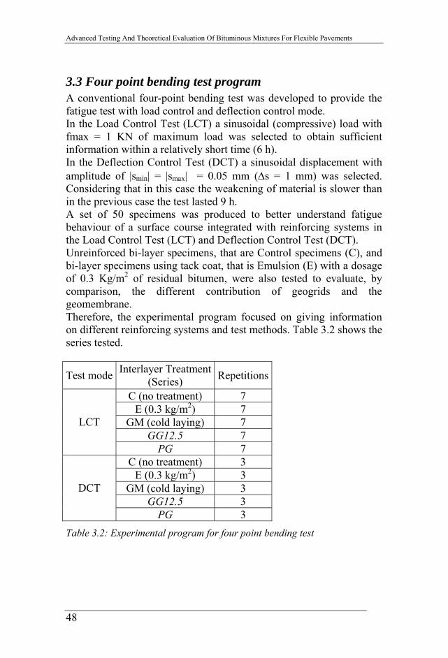
3.3 Four point bending test program A conventional four-point bending test was developed to provide the fatigue test with load control and deflection control mode. In the Load Control Test (LCT) a sinusoidal (compressive) load with fmax = 1 KN of maximum load was selected to obtain sufficient information within a relatively short time (6 h). In the Deflection Control Test (DCT) a sinusoidal displacement with amplitude of |smin| = |smax| = 0.05 mm (∆s = 1 mm) was selected. Considering that in this case the weakening of material is slower than in the previous case the test lasted 9 h. A set of 50 specimens was produced to better understand fatigue behaviour of a surface course integrated with reinforcing systems in the Load Control Test (LCT) and Deflection Control Test (DCT). Unreinforced bi-layer specimens, that are Control specimens (C), and bi-layer specimens using tack coat, that is Emulsion (E) with a dosage of 0.3 Kg/m2 of residual bitumen, were also tested to evaluate, by comparison, the different contribution of geogrids and the geomembrane. Therefore, the experimental program focused on giving information on different reinforcing systems and test methods. Table 3.2 shows the series tested.
Test mode Interlayer Treatment(Series) Repetitions
C (no treatment) 7E (0.3 kg/m2) 7
GM (cold laying) 7GG12.5 7
LCT
PG 7C (no treatment) 3
E (0.3 kg/m2) 3GM (cold laying) 3
GG12.5 3DCT
PG 3Table 3.2: Experimental program for four point bending test
48
Chapter 4. Test equipments – Part I
4. Test equipments – Part I The different experimental equipments used in this research project are described in the following paragraphs:
• Paragraph 4.1 describes the compaction method using Roller Compactor
• Paragraph 4.2 describes the shear test equipment ASTRA able to investigate interlayer shear properties of double-layered cylindrical specimens
• Paragraph 4.3 describes the four point bending tester used to investigate dissipated energy and permanent deformation in fatigue tests on double-layered prismatic specimens (beams).
49
Advanced Testing And Theoretical Evaluation Of Bituminous Mixtures For Flexible Pavements
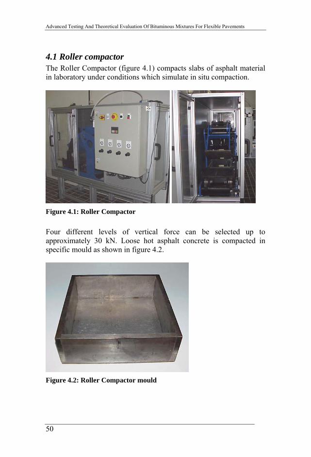
4.1 Roller compactor The Roller Compactor (figure 4.1) compacts slabs of asphalt material in laboratory under conditions which simulate in situ compaction.
Figure 4.1: Roller Compactor
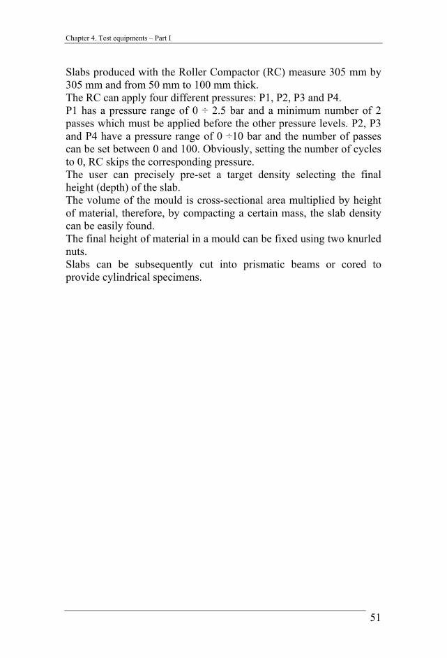
Four different levels of vertical force can be selected up to approximately 30 kN. Loose hot asphalt concrete is compacted in specific mould as shown in figure 4.2.
Figure 4.2: Roller Compactor mould
50
Chapter 4. Test equipments – Part I
Slabs produced with the Roller Compactor (RC) measure 305 mm by 305 mm and from 50 mm to 100 mm thick. The RC can apply four different pressures: P1, P2, P3 and P4. P1 has a pressure range of 0 ÷ 2.5 bar and a minimum number of 2 passes which must be applied before the other pressure levels. P2, P3 and P4 have a pressure range of 0 ÷10 bar and the number of passes can be set between 0 and 100. Obviously, setting the number of cycles to 0, RC skips the corresponding pressure. The user can precisely pre-set a target density selecting the final height (depth) of the slab. The volume of the mould is cross-sectional area multiplied by height of material, therefore, by compacting a certain mass, the slab density can be easily found. The final height of material in a mould can be fixed using two knurled nuts. Slabs can be subsequently cut into prismatic beams or cored to provide cylindrical specimens.
51
Advanced Testing And Theoretical Evaluation Of Bituminous Mixtures For Flexible Pavements
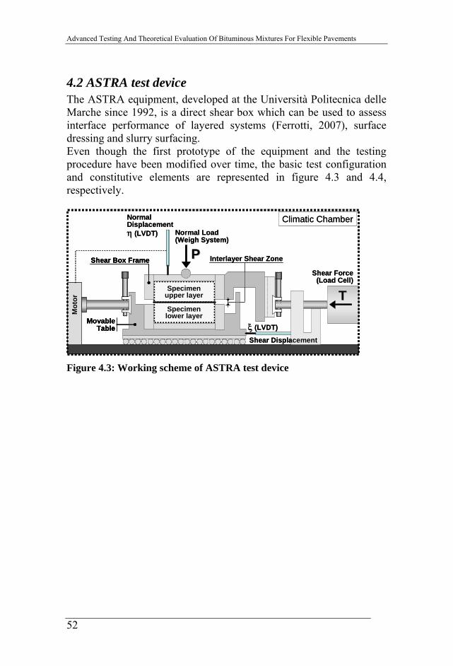
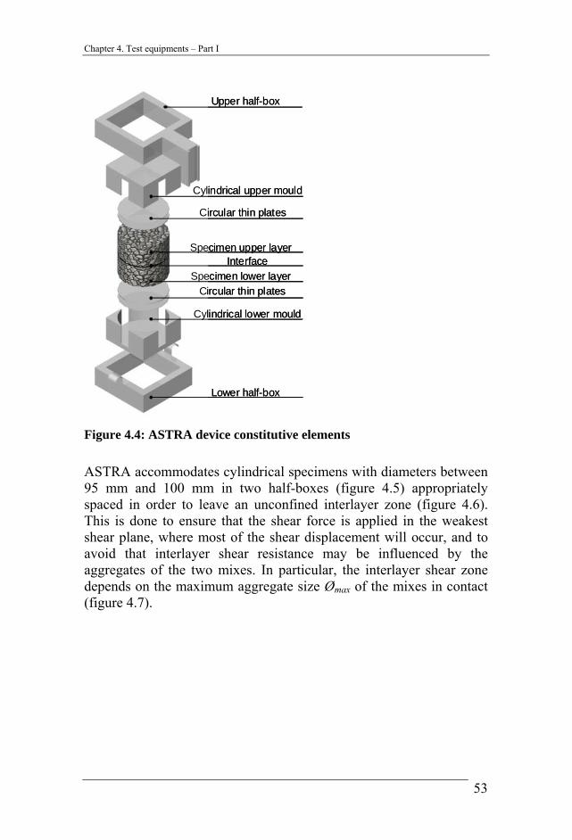
4.2 ASTRA test device The ASTRA equipment, developed at the Università Politecnica delle Marche since 1992, is a direct shear box which can be used to assess interface performance of layered systems (Ferrotti, 2007), surface dressing and slurry surfacing. Even though the first prototype of the equipment and the testing procedure have been modified over time, the basic test configuration and constitutive elements are represented in figure 4.3 and 4.4, respectively.
Specimenupper layer
Specimenlower layer
Climatic ChamberNormalDisplacementη (LVDT) Normal Load
(Weigh System)
PP
TT
Shear Force(Load Cell)
Shear Box Frame
ξ (LVDT)
Shear Displacement
Interlayer Shear Zone
MovableTable
Mot
or
Specimenupper layer
Specimenlower layer
Climatic ChamberNormalDisplacementη (LVDT) Normal Load
(Weigh System)
PP
TT
Shear Force(Load Cell)
Shear Box Frame Shear Box Frame
ξ (LVDT)
Shear Displacement
Interlayer Shear Zone
MovableTable
MovableTable
Mot
or
Figure 4.3: Working scheme of ASTRA test device
52
Chapter 4. Test equipments – Part I
Upper half-box
Cylindrical upper mould
Circular thin plates
Specimen upper layer
Specimen lower layerInterface
Circular thin plates
Cylindrical lower mould
Lower half-box
Upper half-box
Cylindrical upper mould
Circular thin plates
Specimen upper layer
Specimen lower layerInterface
Circular thin plates
Cylindrical lower mould
Lower half-box
Figure 4.4: ASTRA device constitutive elements
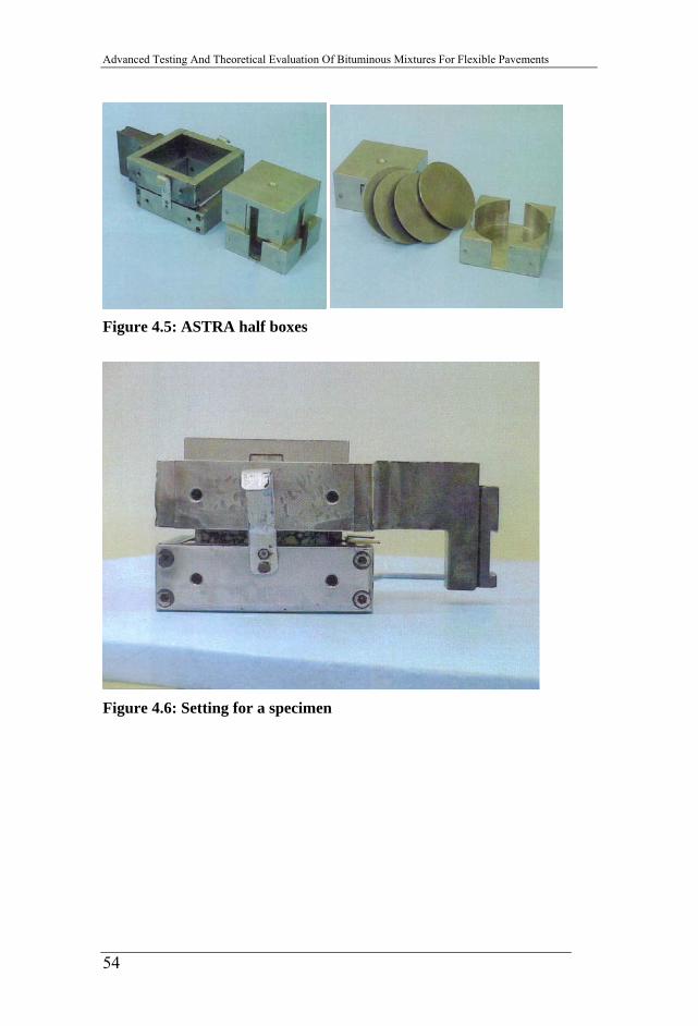
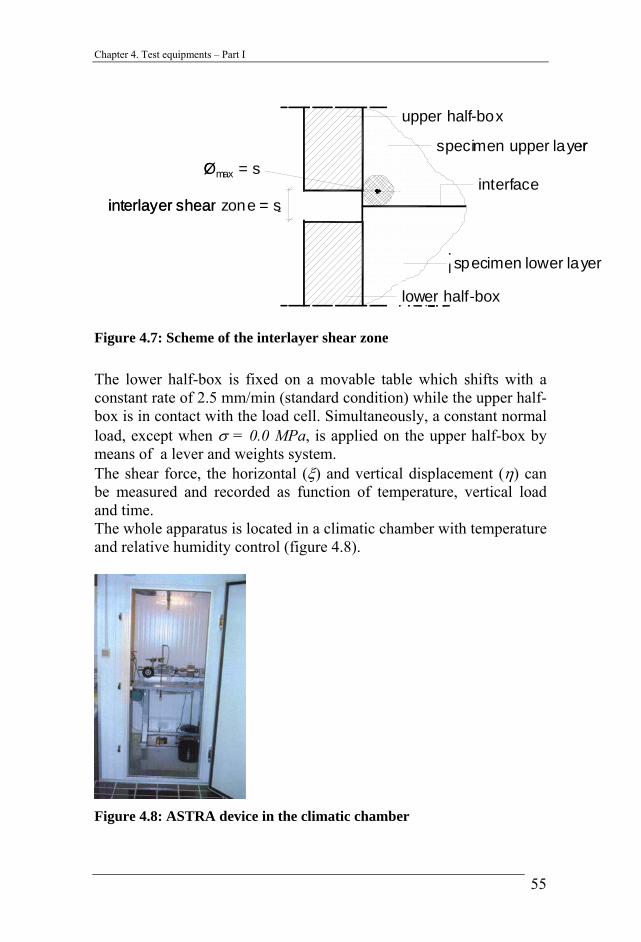
ASTRA accommodates cylindrical specimens with diameters between 95 mm and 100 mm in two half-boxes (figure 4.5) appropriately spaced in order to leave an unconfined interlayer zone (figure 4.6). This is done to ensure that the shear force is applied in the weakest shear plane, where most of the shear displacement will occur, and to avoid that interlayer shear resistance may be influenced by the aggregates of the two mixes. In particular, the interlayer shear zone depends on the maximum aggregate size Ømax of the mixes in contact (figure 4.7).
53
Advanced Testing And Theoretical Evaluation Of Bituminous Mixtures For Flexible Pavements
Figure 4.5: ASTRA half boxes
Figure 4.6: Setting for a specimen
54
Chapter 4. Test equipments – Part I
specimen upper layer
interface
specimen lower layer
lower half-box
interlayer shear zone = s
Ømax = s
upper half-box
specimen upper layer
interface
specimen lower layer
lower half-box
interlayer shear zone = s
Ømax = s
upper half-box
Figure 4.7: Scheme of the interlayer shear zone
The lower half-box is fixed on a movable table which shifts with a constant rate of 2.5 mm/min (standard condition) while the upper half-box is in contact with the load cell. Simultaneously, a constant normal load, except when σ = 0.0 MPa, is applied on the upper half-box by means of a lever and weights system. The shear force, the horizontal (ξ) and vertical displacement (η) can be measured and recorded as function of temperature, vertical load and time. The whole apparatus is located in a climatic chamber with temperature and relative humidity control (figure 4.8).
Figure 4.8: ASTRA device in the climatic chamber
55
Advanced Testing And Theoretical Evaluation Of Bituminous Mixtures For Flexible Pavements
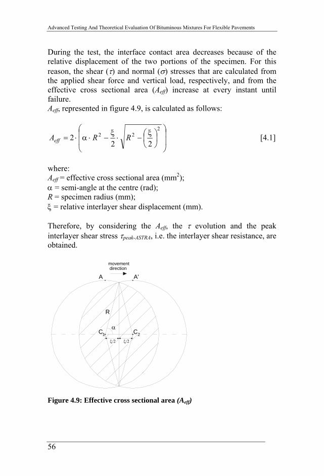
During the test, the interface contact area decreases because of the relative displacement of the two portions of the specimen. For this reason, the shear (τ) and normal (σ) stresses that are calculated from the applied shear force and vertical load, respectively, and from the effective cross sectional area (Aeff) increase at every instant until failure. Aeff, represented in figure 4.9, is calculated as follows:
⎟⎟
⎠
⎞
⎜⎜
⎝
⎛⎟⎠⎞
⎜⎝⎛ ξ
−⋅ξ
−⋅α⋅=2
22
222 RRAeff [4.1]
where: Aeff = effective cross sectional area (mm2); α = semi-angle at the centre (rad); R = specimen radius (mm); ξ = relative interlayer shear displacement (mm). Therefore, by considering the Aeff, the τ evolution and the peak interlayer shear stress τpeak-ASTRA, i.e. the interlayer shear resistance, are obtained.
α
R
C1 2C
A A'
movementdirection
ξ/2ξ/2
Figure 4.9: Effective cross sectional area (Aeff)
56
Chapter 4. Test equipments – Part I
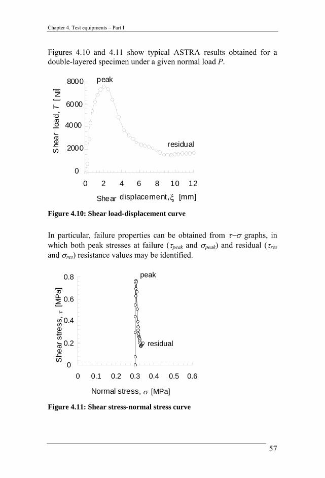
Figures 4.10 and 4.11 show typical ASTRA results obtained for a double-layered specimen under a given normal load P.
0
200
400
600
800
0 2 4 6 8 10 12
Horizontal displacement, δ [mm]
Hor
izon
tal l
oad,
T [k
g]
ξShear
peak
residual
She
arN
0
4000
2000
6000
8000
0
200
400
600
800
0 2 4 6 8 10 12
Horizontal displacement, δ [mm]
Hor
izon
tal l
oad,
T [k
g]
ξShear
peak
residual
She
arN
0
4000
2000
6000
8000
Figure 4.10: Shear load-displacement curve
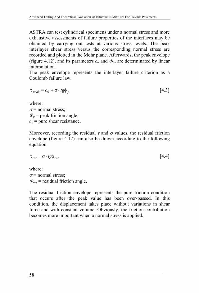
In particular, failure properties can be obtained from τ−σ graphs, in which both peak stresses at failure (τpeak and σpeak) and residual (τres and σres) resistance values may be identified.
0
2
4
6
8
0 1 2 3 4 5 6
Normal stress, σ [kg/cm2]
She
ar s
tress
, τ [k
g/cm
2 ]
0
0.4
0.2
0.6
0.8
0.1 0.2 0.3 0.4 0.50 0.6
[MPa]
[MP
a]
residual
peak
0
2
4
6
8
0 1 2 3 4 5 6
Normal stress, σ [kg/cm2]
She
ar s
tress
, τ [k
g/cm
2 ]
0
0.4
0.2
0.6
0.8
0.1 0.2 0.3 0.4 0.50 0.6
[MPa]
[MP
a]
0
2
4
6
8
0 1 2 3 4 5 6
Normal stress, σ [kg/cm2]
She
ar s
tress
, τ [k
g/cm
2 ]
0
0.4
0.2
0.6
0.8
0.1 0.2 0.3 0.4 0.50 0.6
[MPa]
[MP
a]
residual
peak
Figure 4.11: Shear stress-normal stress curve
57
Advanced Testing And Theoretical Evaluation Of Bituminous Mixtures For Flexible Pavements
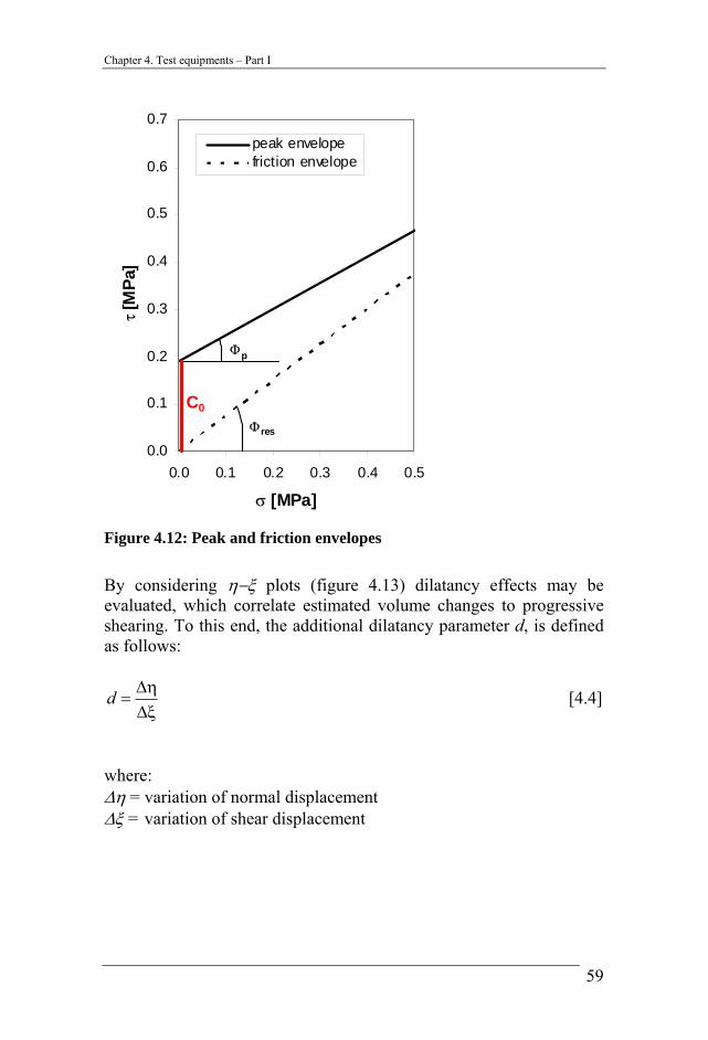
ASTRA can test cylindrical specimens under a normal stress and more exhaustive assessments of failure properties of the interfaces may be obtained by carrying out tests at various stress levels. The peak interlayer shear stress versus the corresponding normal stress are recorded and plotted in the Mohr plane. Afterwards, the peak envelope (figure 4.12), and its parameters c0 and Φp, are determinated by linear interpolation. The peak envelope represents the interlayer failure criterion as a Coulomb failure law.
ppeak tgc φ⋅σ+=τ 0 [4.3] where: σ = normal stress; Φp = peak friction angle; c0 = pure shear resistance. Moreover, recording the residual τ and σ values, the residual friction envelope (figure 4.12) can also be drawn according to the following equation.
resres tgφ⋅σ=τ [4.4] where: σ = normal stress; Φres = residual friction angle. The residual friction envelope represents the pure friction condition that occurs after the peak value has been over-passed. In this condition, the displacement takes place without variations in shear force and with constant volume. Obviously, the friction contribution becomes more important when a normal stress is applied.
58
Chapter 4. Test equipments – Part I
0.0
0.1
0.2
0.3
0.4
0.5
0.6
0.7
0.0 0.1 0.2 0.3 0.4 0.5
s [MPa]
t [M
Pa]
peak envelopefriction envelope
C0
Φres
Φp
σ [MPa]
τ[M
Pa]
0.0
0.1
0.2
0.3
0.4
0.5
0.6
0.7
0.0 0.1 0.2 0.3 0.4 0.5
s [MPa]
t [M
Pa]
peak envelopefriction envelope
C0
Φres
Φp
σ [MPa]
τ[M
Pa]
Figure 4.12: Peak and friction envelopes
By considering η−ξ plots (figure 4.13) dilatancy effects may be evaluated, which correlate estimated volume changes to progressive shearing. To this end, the additional dilatancy parameter d, is defined as follows:
ξ∆η∆
=d [4.4]
where: ∆η = variation of normal displacement ∆ξ = variation of shear displacement
59
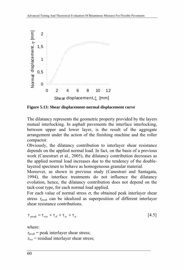
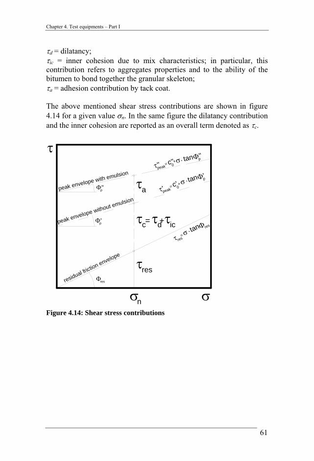
Advanced Testing And Theoretical Evaluation Of Bituminous Mixtures For Flexible Pavements
The dilatancy represents the geometric property provided by the layers mutual interlocking. In asphalt pavements the interface interlocking, between upper and lower layer, is the result of the aggregate arrangement under the action of the finishing machine and the roller compactor. Obviously, the dilatancy contribution to interlayer shear resistance depends on the applied normal load. In fact, on the basis of a previous work (Canestrari et al., 2005), the dilatancy contribution decreases as the applied normal load increases due to the tendency of the double-layered specimen to behave as homogeneous granular material. Moreover, as shown in previous study (Canestrari and Santagata, 1994), the interface treatments do not influence the dilatancy evolution, hence, the dilatancy contribution does not depend on the tack-coat type, for each normal load applied. For each value of normal stress σ, the obtained peak interlayer shear stress τpeak can be idealized as superposition of different interlayer shear resistance contributions.
τd = dilatancy; τic = inner cohesion due to mix characteristics; in particular, this contribution refers to aggregates properties and to the ability of the bitumen to bond together the granular skeleton; τa = adhesion contribution by tack coat. The above mentioned shear stress contributions are shown in figure 4.14 for a given value σn. In the same figure the dilatancy contribution and the inner cohesion are reported as an overall term denoted as τc.
σ σ
τ
τres
τc
τa
τd τic+=
τ'' σc''peak=
+Φ''ptan.
c'τ'peak
=
Φ'. tanσ+p
peak envelope with emulsion
peak envelope without emulsion
resΦ
τres= σ. tan
Φ''p
pΦ'
Φresresidual friction envelope
n
0
0
Figure 4.14: Shear stress contributions
61
Advanced Testing And Theoretical Evaluation Of Bituminous Mixtures For Flexible Pavements
4.3 Four point bending test A conventional four-point bending test (figure 4.15) was developed at the Università Politecnica delle Marche to provide dynamic and static test in load control and deflection control mode on prismatic bituminous specimens.
Figure 4.15: Four point bending test device
This apparatus mainly consists of:
• Servo-hydraulic system and load cell which allow applying load up to 5 KN with a maximum frequency of 5 Hz. The load cell can apply sinusoidal, square and triangular shaped loading wave;
• The extensometer “strain gauge CE-5” (figure 4.16) with measuring range of 0÷5 ± 1%mm. The LVDT controls the vertical displacements at the middle of the specimen and a serial communications port allows the transmission of the data directly to an external computer where data are stored.
• Climatic chamber which allows testing in a temperature range of 0÷40°C ± 0.5°C.
62
Chapter 4. Test equipments – Part I
• The acquisition software, developed at the Università Politecnica delle Marche, is based on discrete Fourier transform and it enables to extrapolate the key parameters, such as vertical displacement, phase angle and dissipated energy as functions of time. Moreover, it allows to filter noise interference and to control non-linear behaviour.
Figure 4.16: Extensometer
63
64
Chapter 5. Result analysis – Part I
5. Result analysis
5.1 Shear test
5.1.1 Introduction As previously mentioned, in this study, three different vertical stresses were applied: σΙ = 0.0 MPa, σΙΙ = 0.2 MPa and σΙΙΙ = 0.4 MPa. Figure 5.1 shows a typical evolution of the shear stress at interface versus the horizontal displacement and highlights the two key values: τpeak and τres.
0.0
0.2
0.4
0.6
0.8
0 2 4 6 8 10 1
ξ [mm]
τ [M
Pa]
2
τpeak
τres
Shea
r stre
ss
Horizontal displacement
0.0
0.2
0.4
0.6
0.8
0 2 4 6 8 10 1
ξ [mm]
τ [M
Pa]
2
τpeak
τres
Shea
r stre
ss
Horizontal displacement
Figure 5.1: Typical shear stress evolution in ASTRA test
As shown in figure 5.2, on a Mohr plain, considering the peak and residual shear stress versus the corresponding vertical stress applied, the peak and residual envelope can be drawn.
65
Advanced Testing And Theoretical Evaluation Of Bituminous Mixtures For Flexible Pavements
σv
τ
τpeak = co + σntanφp
τres = σntanφres
c0
τpeak
τres
σv
τ
τpeak = co + σntanφp
τres = σntanφres
c0
τpeak
τres
Figure 5.2: Peak and residual envelope in the Mohr plain
The peak envelope is represented by the interpolating trend line:
pnpeak c φστ tan0 ⋅+= [5.1] where: τpeak = peak (maximum) shear stress; c0 = pure shear resistance; σn = normal stress applied; φp = peak envelope angle. In a previous study (Canestrari et al., 2005), it has been shown that, for a given σn, the peak shear stress can be obtained by a sum of different shear stress contributions:
τa = interface adhesion. Obviously, if the emulsion is not applied, the term τa disappears. Taking into account the residual shear stress versus the corresponding normal stress applied at the interface, the residual envelope can also be plotted on a Mohr plain (figure 5.2). Therefore, the constitutive law after failure is the following:
resnres φστ tan⋅= [5.3] where: τres = residual shear stress; σn = normal stress; φres = residual friction angle. When a geomembrane is placed at the interface, the previous equation changes as follows:
resnres c φστ tan1 ⋅+= [5.4] where: c1 = pure shear resistance after the failure.
5.1.2 CIC evaluation Six different interlayer configurations are investigated in this paragraph as detailed in table 3.1. Figures 5.3 and 5.4 illustrate the peak and the residual envelopes studied for all interlayer configurations.
67
Advanced Testing And Theoretical Evaluation Of Bituminous Mixtures For Flexible Pavements
τpeak = 0,29σpeak + 0,51R2
peak = 0,42
τpeak = 0,49σpeak + 0,57R2
peak = 0,72
0.0
0.2
0.4
0.6
0.8
0.0 0.2 0.4 0.6σpeak (MPa)
peak
(MPa
)
C EC Peak envelope E Peak envelope
τres = 0,78σres
R2res = 0,92
τres = 0,75σres
R2res = 0,97
0.0
0.2
0.4
0.6
0.0 0.2 0.4 0.6σres (MPa)
res (
MPa
)
C EC Res. envelope E Res. envelope
Figure 5.3: Peak and residual envelopes – C and E (0.3 kg/m2) series
Figure 5.4: Peak and residual envelopes – GM (cold lay), GG12.5, GG25 and PG series
69
Advanced Testing And Theoretical Evaluation Of Bituminous Mixtures For Flexible Pavements
In order to facilitate the assessment in table 5.1 the key parameters for each interlayer configurations has been listed. In particular, table 5.1, for C and E series, confirms a previous research (Canestrari et al., 2005) which stated that the residual friction angle φres varies from 36° to 40°. The meaning could be that, without integration of reinforcement, the residual friction angle appears as an intrinsic property of the materials in contact, which only depends on their own characteristics. It is interesting to note that the residual friction angle φres of GG12.5 and GG25 series is still included within the mentioned range. The open mesh size of GG12.5 and GG25 actually allows contact between the upper and lower layer. Therefore φres is still related to the individual characteristics of the two layer materials in contact and their values are slightly higher compared to the C and E series as a consequence of the presence of the grid elements. On the contrary this is not true for GM and PG series. In fact, GM and PG do not allow real contact between the surrounding materials. Thus, in these cases, φres is influenced by reinforcement characteristics. In particular, observing the reinforced specimens with GM after testing, the failure clearly concerned only the geomembrane: the two asphalt layers shifted each other without breaking and the textile was completely torn and separated from its bitumen coating. Table 5.1 shows that in the GM series pure shear resistance after failure is not absent (c1 ≠ 0). This could be explained by considering residual resistance after failure also in terms of cohesion.
τpeak = c0 + σn tan φp τres = c1+ σ tan φresInterlayer treatment T (°C)
φp (°) c0 (MPa) φres (°) c1 (MPa) C (no treatment) 20 16.4 0.505 38.1 /
PG 20 47.4 0.060 44.8 / Table 5.1: Summary of key parameters in CIC systems
Figures 5.3 and 5.4 show that the highest shear resistance is generally obtained by E series. All reinforcement systems offer lower shear resistance. In particular, it can be supposed that geogrid affects the
70
Chapter 5. Result analysis – Part I
interlayer interaction and generates a separation layer (Caltabiano and Brunton, 1991, Brown et al., 2001), on the other hand, geomembrane produces a deformable film. Considerable results are obtained only with GG25 series because of its relatively wide mesh-size. The peak envelope angle φpeak indicates how the shear resistance changes as a function of the applied normal stress (high φpeak value means strong influence of normal stress applied on the shear resistance). As reported in table 5.1, all geogrid series denote a significant influence of normal stress showing a more sensitive behaviour in comparison with the other series. A geogrid causes discontinuity between upper and lower layers but, increasing the normal load, the interaction among surrounding materials and geogrid ribs generates a significant mechanical interlocking which could balance the disadvantages due to the discontinuity. This does not happen for the GM series that shows the lowest φpeak value. Obviously, its inner textile inhibits mechanical interlocking. By comparing pure shear resistance c0 in case of reinforced systems, a decrease from 26% up to 90% with respect to E series can be assessed. Reinforcement systems as geogrids and geomembrane appear to generate a weakened interlayer that damages the pure shear performance. From figures 5.3 and 5.4, it can be observed that, except for the PG series, the residual friction angle is higher than the peak envelope angle (φres > φpeak) implying a substantial convergence of residual and peak envelopes. It seems that under high confining normal stresses, in accordance with energy-based predictions, dilatancy contribution tends to be negligible and the overall behaviour does not depend on interlayer properties but can be expressed as a function of the asphalt mixes.
5.1.3 CIP evaluation According with the experimental program listed in table 3.1, three different interlayer configurations have been studied. Figures 5.5 and 5.6 show the peak and the residual envelopes for all interlayer configurations considered at 20 and 40 °C, respectively.
71
Advanced Testing And Theoretical Evaluation Of Bituminous Mixtures For Flexible Pavements
Figure 5.6: Summary of peak and residual envelopes – T = 40°C
73
Advanced Testing And Theoretical Evaluation Of Bituminous Mixtures For Flexible Pavements
The main information related to the previous figures are reported in tables 5.2 and 5.3. As shown in previous study (Canestrari et al., 2005) and in the previous paragraph, the residual friction angle φres in CIC configurations varies from 36° to 40° except for GM and PG series. As expected, underlining once again that material characteristics influence φres, in CIP system with emulsion at interlayer, φres is not included in this range. In particular, it becomes 44.85° and 42.41° at 20 °C and 40 °C, respectively. The different types of surrounding materials and the high tack coat dosage (1.2 kg/m2) could influence the friction at the interlayer. Probably, a higher percentage of big-sized aggregates provides more resistance to horizontal displacement. As previously stated, also in CIP specimens, with GM (in both laying conditions), φres results are lower than E series values confirming that, in this case, φres is still influenced by reinforcement characteristics. Moreover, φres keeps the same magnitude order of the correlated configuration in CIC system again, validating the hypothesis that it could depend on geomembrane properties.
τpeak = c0 + σn tan φp τres = c1+ σ tan φresInterlayer treatment T (°C) φp (°) c0 (MPa) φres (°) c1 (MPa)
GM (warm laying) 40 19.42 0.040 19.44 0.038 Table 5.3: Summary of key results at 40°C
For reinforced specimens with GM at both temperatures, the presence of pure shear resistance after failure (c1 ≠ 0) can be noted. Therefore, the geomembrane provides shear resistance even after the interlayer failure as well as in CIC system. It is important to remark that at 20 °C
74
Chapter 5. Result analysis – Part I
the c1 value is three times higher than in the CIC system. Even in this case the double-layered system composition is the only difference. Hence c1 also depends on material properties. At 40 °C c1 values for both GM series tend to disappear because of a general system weakening. Figure 5.5 shows that, in both GM series at 20 °C, shear resistance is higher than in E series for normal stresses up to about 0.2 MPa. Over this threshold the E series shows higher shear performance. Therefore, the use of geomembrane for heavy traffic loads would not be recommended. As shown in figure 5.6, at 40 °C the peak envelope, i.e. shear resistance, related to E series is generally over both GM envelopes. The consequence is that the use of geomembrane for roads subjected to high temperature would not be advisable. Degradation could become significant even under low traffic volumes. The peak envelope angle φpeak, for both temperatures, in E series is still higher than that in GM series as observed for CIC system. Consequently, the higher the normal stress applied, the higher the tack coat benefits in terms of shear resistance. Moreover, it can be noted that at 20 °C φpeak in GM series for CIP system is slightly higher than that for CIC system. This phenomenon could be due to larger amount of big-sized aggregates in the upper layer which can interlock better with the lower geomembrane interlayer. Contrary to the CIC system results, in both GM series pure shear resistance c0 is higher than in E series. In particular, at 20 °C the pure shear resistance of E series is about 70% of GM series while at 40 °C pure shear resistance of E series is about 85% of GM series. This factor is strongly influenced by the materials used in double-layered systems, too. The shear performance at 40 °C is significantly lower than that obtained at 20 °C for all interlayer configurations studied. This general weakening due to temperature effects has been observed in all CIP systems, but it is very clear in the GM series noting that the respective peak and residual envelopes almost coincide with each other (figure 5.6). The reason could be justified as a viscosity reduction of the geomembrane coating bitumen with a consequent increasing deformability at high temperature. For a better evaluation of temperature effects on mechanical behaviour, figures 5.7, 5.8 and 5.9 represent the peak shear stress as a
75
Advanced Testing And Theoretical Evaluation Of Bituminous Mixtures For Flexible Pavements
function of temperature for E series, GM (cold laying) series and GM (warm laying) series, respectively.
E τpeak = -0.010T + 0.820
τpeak = -0.012T + 0.730
τpeak = -0.009T + 0.3700
0.2
0.4
0.6
0.8
0 20 40 T [°C]
peak
[MPa
]
= 0,0 MPa = 0,2 MPa = 0,4 MPaσσ
σ
E τpeak = -0.010T + 0.820
τpeak = -0.012T + 0.730
τpeak = -0.009T + 0.3700
0.2
0.4
0.6
0.8
0 20 40 T [°C]
peak
[MPa
]
= 0,0 MPa = 0,2 MPa = 0,4 MPaσσ
σ
Figure 5.7: Influence of temperature on φpeak – E (1.2 kg/m2) series
GM (cold laying)τpeak = -0.011T + 0.680
τpeak = -0.013T + 0.640
τpeak = -0.012T + 0.540
0
0.2
0.4
0.6
0.8
0 20 40 T [°C]
peak
[MPa
]
= 0,0 MPa = 0,2 MPa = 0,4 MPaσ
σσ
GM (cold laying)τpeak = -0.011T + 0.680
τpeak = -0.013T + 0.640
τpeak = -0.012T + 0.540
0
0.2
0.4
0.6
0.8
0 20 40 T [°C]
peak
[MPa
]
= 0,0 MPa = 0,2 MPa = 0,4 MPaσ
σσ
Figure 5.8: Influence of temperature on φpeak – GM series
76
Chapter 5. Result analysis – Part I
GM (warm laying)
τpeak = -0.011T+0.640
τpeak =-0.013T+0.630
τpeak =-0.012T+0.520
0
0.2
0.4
0.6
0.8
0 20 40 T [°C]
peak
[MPa
]
= 0,0 MPa = 0,2 MPa = 0,4 MPaσ
σσ
GM (warm laying)
τpeak = -0.011T+0.640
τpeak =-0.013T+0.630
τpeak =-0.012T+0.520
0
0.2
0.4
0.6
0.8
0 20 40 T [°C]
peak
[MPa
]
= 0,0 MPa = 0,2 MPa = 0,4 MPaσ
σσ
Figure 5.9: Influence of temperature on φpeak – GM series
In figures 5.7, 5.8, 5.9, it can be noted that under constant normal stress level, shear resistance decreases with the increase in temperature. Moreover, the lines reported in each graphs are quite parallel highlighting that the decreasing of φpeak from 20 °C to 40 °C, is not related to applied normal stress and, hence, the reduction cannot be attributed to friction contribution. These evolutions are similar to those in CIC systems as investigated in a previous research (Canestrari et al., 2005). Therefore, the surrounding material does not influence the φpeak decreasing behaviour from 20 °C to 40 °C. Finally, by comparing the envelopes in both temperatures (figure 5.5 and 5.6), it can be asserted that the laying technique for geomembrane does not affect the shear performance significantly. Hence the cold laying generally used in situ for geomembranes does not influence the interlayer performance negatively.
77
Advanced Testing And Theoretical Evaluation Of Bituminous Mixtures For Flexible Pavements
5.2 Four point bending test
5.2.1 Deflection control test A new setting was developed to provide a Deflection Control Test (DCT). In DCT when microcracks are generated and material resistance decreases, the load-applied also decreases to obtain constant deflection. In this way, it is possible to analyse the fatigue behaviour, even if defining fatigue failure is often difficult. In this case, the results were analysed using the dissipated energy as a key parameter. The dissipated energy for a cycle is defined as the area within the stress-strain hysteresis loop or, in other words, as the difference between the amount of energy put into the material and the amount of energy recovered. Theoretically, considering a stress-strain curve for elastic material, the load and unload evolution are coinciding. Therefore the total amount of energy put into the material coincides with the amount of energy recovered. Damage does not affect the material. For visco-elastic materials the load curve does not correspond with the unload curve, thus a hysteresis loop is generated. In this case damage is progressively accumulated in the material. The main advantage of this approach is its simplicity. Only special data acquisition equipment is required. The acquisition software measures load, vertical displacement and phase angle. Dissipated energy is calculated as follows:
iiii sFG ρπ sin⋅⋅⋅= [5.5] where: Gi = dissipated energy during ith cycle; Fi = the load-applied amplitude at ith cycle; si = the displacement amplitude at ith cycle; ρi = the phase angle between the load and displacement wave signals at ith cycle. Several authors (Al-Khateeb & Shenov, 2004, Daniel et al., 2004, Ghuzlan & Carpenter, 2000, Van Dijk, 1975) have already investigated the criteria of energy-based fatigue failure.
78
Chapter 5. Result analysis – Part I
In this research, the main disadvantages in DCT method were that either a longer time was required to obtain material failure or the fracture was not clear, hence, only the decreasing mechanical properties were evaluated. With equation [5.5], it was possible to calculate the dissipated energy for each cycle. In order to simplify the data analysis, a mean value of dissipated energy at fixed intervals was plotted as a function of the number of cycles. It is well known that, in DCT the dissipated energy decreases as the number of cycles increases. Initially, the dissipated energy quickly decreases implying rapid alteration of material. After this first phase the decreasing rate tends to turn to a constant level as does the damage evolution. Based on equation [5.5], this process means that to obtain the fixed and constant deflection, the applied load decreases as a function of the number of cycles. The decrease in the applied load to reach the same deflection implies that deterioration of the material is in action. Even if only a part of dissipated energy damages the material, the use of evolution of dissipated energy is appropriate to describe the progress of damage. Therefore, damage effects can be studied by means of the dissipated energy theory. As previously mentioned, load and phase angle changes during the test causing a change in dissipated energy. A parameter R is introduced which is the ratio between the mean value of dissipated energy in the final interval (Efin) and that in the initial interval (Ein). Therefore, R is formulated as follows:
100EE
Rin
fin ⋅= [5.6]
This parameter recognizes structural alteration in the material. Low R value means that the deterioration process has seriously affected the material. The Mean R of each series was taken into account to compare the performance of different kinds of interface configuration. Table 5.4 shows all data obtained from DCT.
79
Advanced Testing And Theoretical Evaluation Of Bituminous Mixtures For Flexible Pavements
Series Specimen Ein[J]
Mean Ein [J]
Efin[J]
Mean Efin [J]
Mean R [%]
C1 0.07 0.04 C2 0.11 0.05 C C3 0.06
0.08 0.04
0.04 50
E1 0.13 0.09 E2 0.11 0.07 E E3 0.08
0.11 0.07
0.07 64
GM1 0.07 0.06 GM2 0.09 0.08 GM GM3 0.06
0.07 0.05
0.06 86
GG1 0.10 0.07 GG2 0.08 0.06 GG12.5 GG3 0.07
0.08 0.04
0.06 75
PG1 0.07 0.06 PG2 0.07 0.06 PG PG3 0.07
0.07 0.06
0.06 86
Table 5.4: Energy-related data for all series in DCT
To facilitate the assessment figure 5.10 illustrates the Mean Ein and Mean Efin values for each series and figure 5.11 shows the Mean R results for each series.
0.08
0.11
0.070.08
0.070.060.060.06
0.07
0.04
0
0.04
0.08
0.12
C E GM GG PGInterface configuration
Diss
ipat
ed E
nerg
y [J
]
Mean Ein [J] Mean Efin [J] Figure 5.10: Mean Ein and Mean Efin for each series
80
Chapter 5. Result analysis – Part I
50
64
86
75
86
0
20
40
60
80
100
C E GM GG PGInterface configuration
Mea
nR
[%]
50
64
86
75
86
0
20
40
60
80
100
C E GM GG PGInterface configuration
Mea
nR
[%]
50
64
86
75
86
0
20
40
60
80
100
C E GM GG PGInterface configuration
Mea
nR
[%]
Figure 5.11: Mean R for each series
In figure 5.10, it can be noted that all reinforced series and C series have lower Ein values than that in E series. This means that the E series seems to be less deformable at the beginning. Therefore, reinforced asphalt systems (GM, PG and GG12.5) are not as stiff as asphalt system with tack coat (E) and this leads us to assert that a geosynthetic at the interface generates separation between upper and lower layer confirming previous research on geosynthetic shear performance at the interface (Bocci et al. 2006). However, at the end of the test, the dissipated energy in E series drops considerably showing lower values of Mean R (figure 5.11). After the test, reinforced series and E series have almost the same values of dissipated energy of reinforced systems. Therefore, damage drastically affects E series. Probably, if the test had been longer, the decrease in dissipated energy for E series would have been even worse. It is also important to note that, in spite of GM works as stress absorbing system and PG and GG12.5 work as reinforcing system, GM, PG and GG12.5 series have significantly high Mean R values (figure 5.11). This means that the level of dissipated energy is quite stable, and consequently that the mechanical properties do not change significantly during the test, hence, the damage process is delayed.
81
Advanced Testing And Theoretical Evaluation Of Bituminous Mixtures For Flexible Pavements
5.2.2 Load control test A repeated application of heavy traffic loads, associated with severe environmental conditions, can generally be considered as the most important cause of pavement asphalt degradation. While a material is being subjected to cyclic loading, degradation principally occurs in terms of reduction of storage or dissipation capacity of internal energy, decrease of modulus, and development of permanent deformation. Several fatigue tests are employed in order to assess the behaviour of bituminous materials under repeated load applications. Fatigue tests can be summarized (Di Benedetto et al., 1996; Di Benedetto et al., 1998; Di Benedetto et al., 2004) on the basis of their test configurations (bending tests, tension-compression tests and shear tests) or stress distribution (homogenous and non homogenous). In any case, fatigue failure is “a point at which the specimen is unable to continue to perform in a satisfactory manner” (Pell, 1973). Therefore, fatigue performance can be determined by analysing different parameters and using different approaches. It depends on which characteristic is investigated and/or which is the available test device. As previously described, in LCT a sinusoidal load was applied and the corresponding vertical displacements were measured. In LCT the compressive load wave is kept constant causing a progressive increase of strain and, after the initial fracture, the stress concentration in the fracture tip generates rapid cracking through the whole layer. This is due to a decreasing resisting section while the applied load keeps the initial magnitude. In this mode the stress will break the specimen at the end of the test. Therefore, it could be easy to define failure as complete fracture of the specimen. Figure 5.12 shows a typical evolution of the vertical displacement as a function of number of cycles during the test on unreinforced specimen.
82
Chapter 5. Result analysis – Part I
0
2
4
6
8
10
0 5000 10000 15000 20000Number of loading cycles
Verti
cal d
ispl
acem
ent
[mm
]C9
Figure 5.12: Vertical displacement versus number of cycles during a typical LCT
However, in this study, using reinforcement systems, the complete fracture of the specimen would require a longer test period or too high load level. Therefore an alternative approach was used. The typical evolution of a fatigue test, apart from the type of test configuration and approach used, has three distinct phases. The first phase is characterized by a decreasing rate evolution. This phenomenon can be physically explained as a redistribution of stress, resetting of material, hardening, and healing. In the second phase, the evolution rate becomes almost constant showing an approximate linear relationship with time. This phase corresponds to initiation and propagation of microcracks. Finally, in the third phase macrocracks begin to develop and the evolution rate progressively increases up to complete fracture of specimen. Several authors have defined failure criteria as the point at which a specific geometrical property of a fatigue evolution curve changes, implying a change in the evolution phase. For instance, a previous study (Ghuzlan et al., 2000) defined the ratio between instantaneous change in dissipated energy and total energy as the key factor for the failure criterion. They determined the failure as “the number of load cycles at which the change in this energy ratio begins to increase rapidly”. This point could represent the border between the second and third phase. Whereas, based on the definition of the energy ratio (Van Dijk et al., 1977), another author (Rowe, 1993) has defined the failure criterion as “the point at which the slope of the energy ratio versus number of load cycles deviates from a
83
Advanced Testing And Theoretical Evaluation Of Bituminous Mixtures For Flexible Pavements
straight line”. This point could represent the microcrack initiation phase. On the other hand, other authors (Francken, 1977; Bodin et al., 2002) has suggested that the first phase could be described by means of a power law whereas the second and third phase by an exponential law. One of the purposes of this experimental project is to suggest a consistent failure criterion for fatigue tests considering the previous remarks as a starting point. To this end, this work proposes to distinguish two main phenomena in fatigue test: hardening and damage. For asphalt concrete, hardening could be defined as reorientation and resetting of material, and damage could be identified as deterioration and reduction of resistance performance. In particular, it can be asserted that hardening is a limited phenomenon, i.e. it can not occur ad infinitum (Scarpas et al., 1997), and damage occurs over a threshold (Lemaitre, 1996). These two phenomena tightly coexist and they cannot be separated directly. However, the point at which hardening becomes negligible and damage begins to significantly propagate can be established as a failure criterion. It can be assumed that before this point, damage can be ignored and beyond this point hardening phase ends. The flex point of a permanent deformation curve can be stated as the separation or balance point between these two different contributions. Therefore, a failure criterion can be defined by the number of load cycles (or time) required to reach the flex point in a permanent deformation curve εp(t). Obviously, under the same testing conditions, the permanent deformation evolution curve depends on the material behaviour and, in particular, figure 5.13 compares a typical permanent deformation evolution curve for unreinforced specimen with one for reinforced specimen. Moreover, in this figure hardening and damage phase can be clearly distinguished in both cases.
84
Chapter 5. Result analysis – Part I
0
2
4
6
8
10
0 5000 10000 15000 20000Number of loading cycles
Verti
cal d
ispl
acem
ent
[mm
]C9 Flex point
Hardening phase
Damage phase
0
2
4
6
8
10
0 5000 10000 15000 20000Number of loading cycles
Verti
cal d
ispl
acem
ent
[mm
]C9 Flex point
Hardening phase
Damage phase
0
2
4
6
8
10
0 5000 10000 15000 20000Number of loading cycles
Verti
cal d
ispl
acem
ent
[mm
]
GM5 Flex point
Hardening phase Damage phase
0
2
4
6
8
10
0 5000 10000 15000 20000Number of loading cycles
Verti
cal d
ispl
acem
ent
[mm
]
GM5 Flex point
Hardening phase Damage phase
Figure 5.13: Comparison between εp evolution for unreinforced and reinforced specimen
From a mathematical point of view, the flex point is defined as the point where the second derivative turns its sign. In this case, the flex point was found as the minimum value of the parabola that interpolates the slope curve of the vertical displacement. In regard to previous figure 5.3, the following figure 5.14 shows the minimum value of the parabola that interpolates the slope curve of the permanent deformation evolution for an unreinforced and reinforced specimen.
85
Advanced Testing And Theoretical Evaluation Of Bituminous Mixtures For Flexible Pavements
Figure 5.14: Interpolation of slope curve in LCT by means of a parabola in order to find the minimum.
The number of cycles corresponding to the flex point (Nf) was considered as a representative parameter. In this way this number of cycles was related to the failure of the specimen. In order to facilitate the assessment of the fatigue behaviour an Improvement Ratio is introduced (IR). IR is defined as follows:
100N
NNIR C
f
Cf
thf ⋅
−= [5.7]
where is the number of cycles corresponding to the flex point of i
thfN
th series and is the number of cycles corresponding to the flex point of C series.
CfN
86
Chapter 5. Result analysis – Part I
In figure 6.15, it can be noted that IR is able to discriminate between different interface configurations. All reinforced series (GM, GG12.5 and PG) and the series with tack coat (E) extend fatigue life compared with the control series (C). In particular, E series shows an enhancement in fatigue life by 85%. Reinforced systems appear to be particularly effective under these conditions with an enhancement in fatigue life from 159% to 174%. Moreover, also the Vertical Displacement (VD) corresponding to Nf was taken into account. Figure 5.16 illustrates the mean VD results for each series.
85
174162 159
0
50
100
150
200
E GM GG PGInterface configuration
Impr
ovem
entR
atio
IR [%
]
85
174162 159
0
50
100
150
200
E GM GG PGInterface configuration
Impr
ovem
entR
atio
IR [%
]
85
174162 159
0
50
100
150
200
E GM GG PGInterface configuration
Impr
ovem
entR
atio
IR [%
]
Figure 5.15: Improvement ratio (IR) for each series
5.554.88 4.53
5.66.55
0
2
4
6
8
C E GM GG PGInterface configuration
Verti
calD
ispl
acem
entV
D
[mm
]
5.554.88 4.53
5.66.55
0
2
4
6
8
C E GM GG PGInterface configuration
Verti
calD
ispl
acem
entV
D
[mm
]
5.554.88 4.53
5.66.55
0
2
4
6
8
C E GM GG PGInterface configuration
Verti
calD
ispl
acem
entV
D
[mm
]
Figure 5.16: Vertical displacement at flex point for each series
87
Advanced Testing And Theoretical Evaluation Of Bituminous Mixtures For Flexible Pavements
By combining both IR and VD results at the flex point, important remarks can be deduced in order to explain the different behaviour of geomembrane and geogrid in asphalt concrete. As previously showed in figure 5.15, based on flex point failure criteria, all reinforced systems have high IR values, hence high fatigue performance in comparison to C and E series. However, by comparing the vertical displacement at the flex point, GM series shows the lowest values (figure 5.16). On the contrary, GG12.5 and PG series show high values of VD at the flex point (figure 5.16). Therefore, GM allows to extend fatigue life and to distribute loads better keeping low values of VD. GG and PG show considerable fatigue performance but also high values of VD, instead. Geogrid in asphalt system is used to give a contribution to tensile resistance but probably in this case GG12.5 and PG begin to act only when high VD values are reached resulting less effective than GM. Probably, with low VD values, that is with low beam inflexion, low tensile stress acts at interface and as such geogrid does not give a substantial contribution. It begins to work only when either the maximum tensile resistance of asphalt concrete is reached or the crack tip grows up to geogrid ribs. This means that high values of VD are required. As asserted by other authors (Brown et al. 2001), the best contribution of geogrid against cracking and fatigue damage is achieved when geogrid is placed where the tensile stress is maximum, this is, at the bottom of bound layers. On the contrary, geomembrane appears effective against cracking and fatigue failure even if it is placed at about mid-depth.
88
Chapter 5. Result analysis – Part I
5.2.3 Integrated fatigue model for LCT In order to find the flex point by means of the minimum of the parabola that interpolates the slope curve )(tpε& (Bocci et al., 2007) is often difficult because of scattering in data acquisition or technical problems to filter every interference and an uncorrected evaluation of the minimum could lead to considerable wrong assessment of Nf as shown in figure 5.17.
y = 4.94760E-12x2 - 8.77757E-08x + 6.99678E-04R2 = 9.38194E-01
0
0.0002
0.0004
0.0006
0.0008
0 5000 10000 15000 20000Number of cycles
Slop
e
y = 4.94760E-12x2 - 8.77757E-08x + 6.99678E-04R2 = 9.38194E-01
0
0.0002
0.0004
0.0006
0.0008
0 5000 10000 15000 20000Number of cycles
Slop
e
NfI Nf
II
y = 4.94760E-12x2 - 8.77757E-08x + 6.99678E-04R2 = 9.38194E-01
0
0.0002
0.0004
0.0006
0.0008
0 5000 10000 15000 20000Number of cycles
Slop
e
y = 4.94760E-12x2 - 8.77757E-08x + 6.99678E-04R2 = 9.38194E-01
0
0.0002
0.0004
0.0006
0.0008
0 5000 10000 15000 20000Number of cycles
Slop
e
y = 4.94760E-12x2 - 8.77757E-08x + 6.99678E-04R2 = 9.38194E-01
0
0.0002
0.0004
0.0006
0.0008
0 5000 10000 15000 20000Number of cycles
Slop
e
y = 4.94760E-12x2 - 8.77757E-08x + 6.99678E-04R2 = 9.38194E-01
0
0.0002
0.0004
0.0006
0.0008
0 5000 10000 15000 20000Number of cycles
Slop
e
NfI Nf
II
Figure 5.17:Possible uncorrected evaluation of the minimum
In this context a descriptive model (Virgili et al., 2007), based on a classic power law, is presented. A descriptive model is a mathematical tool that describes and simulates the behaviour of a specific system. In this study the evolution model aims to reproduce the observed response of an asphalt concrete mixture under different ranges and modes of excitation filtering unexpected scattering of data which depends on external and random causes. The proposed mathematical model allows to find, without ambiguity, the flex point of a permanent deformation curve during a fatigue test; thus the failure point can be specified accurately. However the equation parameters lack physical interpretation. For this reason, though the mathematical model is remarkably good fit to measured permanent deformation curves, it has no predictive power beyond the testing time.
89
Advanced Testing And Theoretical Evaluation Of Bituminous Mixtures For Flexible Pavements
Obviously, this model can also be applied to determine the permanent deformation in creep tests. Further studies are going to present the application of the same model in creep tests as well. The study focused on the development of a mathematical model that is able to define the permanent deformation evolution of a specimen during a fatigue test by means of two boundary values and a shape function. Moreover, such model does not use a threshold for permanent deformation. The starting point is the use of the well-known power law to identify the permanent deformation evolution.
bp ta ⋅=ε [5.8]
where: εp = the permanent deformation, t = time, a and b = material parameters. Equation [5.9] can be easily deduced from equation [5.8]:
ppp
tb
dtd
εεε
⋅== & [5.9]
moreover from equation [5.8], it can be noted that:
b1
p
at ⎟
⎟⎠
⎞⎜⎜⎝
⎛=
ε [5.10]
by substituting equation [5.10] in equation [5.9]:
( )b11
pb
1
b1
p
pp ab
a
b −⋅⋅=
⎟⎠
⎞⎜⎝
⎛
⋅= ε
ε
εε& [5.11]
as mentioned above, b and a are material parameters, hence:
Cb11Aab b
1=−=⋅ ; [5.12]
90
Chapter 5. Result analysis – Part I
by substituting equations [5.12] in equation [5.11]:
Cpp A εε ⋅=& [5.13]
where:
pε& = the permanent deformation rate, A and C = material parameters. Considering that permanent deformation is directly related to damage (Lemaitre, 1996), equation [5.13] appears very similar to the damage relationship used by Bodin (Bodin et al., 2002) which is able to predict the first phase of fatigue test. Further developments have been carried out by the same authors (Bodin et al., 2006) in order to consistently simulate the second and the third fatigue phase also. In fact, regardless of the loading and testing mode, the damage growth may be assumed proportional to the power law of damage itself during the first phase of a fatigue test and proportional to the exponential law of damage itself during the second and third phase of a fatigue test (Bodin et al., 2006). In order to obtain a unique analytical law able to represent the overall fatigue behavior, a new function H is introduced as follows:
( )C
p
pCp CHH
ε
εε
&& ⋅−=⇒= − 1)1( [5.14]
replacing equation [5.13] in [5.14], a linear equation determines H:
( ) AC1H ⋅−=& [5.15] Equation [5.15] can also be expressed in terms of an equation of first degree:
( ) ( )0101 ttAC1HH −⋅⋅−+= [5.16] therefore H(t) is a linear function of time and ( ) AC1 ⋅− defines its slope. Considering three different values of H(t) in succession and with ∆t as time period, it can be asserted:
91
Advanced Testing And Theoretical Evaluation Of Bituminous Mixtures For Flexible Pavements
2i1ii2i1i1ii HH2H
tHH
tHH
−−−−− −=⇒
∆−
=∆− [5.17]
using the definition of H in equation [5.17], the incremental equation in terms of permanent deformation can be obtained as follows:
( ) ( )[ ] CipipipCC
−−−
−−−= 1
1
)2()1()(11
2 εεε [5.18] Hypothesizing that C slowly changes in a narrow and fixed interval during a test, it can be taken as a shape function that allows to simulate the evolution of permanent deformation in a fatigue test. In fact, all these three phases of a fatigue test can be simulated by C as a time-dependent function. This incremental equation allows to plot the permanent deformation evolution in a fatigue test and to filter the scattering data in experimental tests. The incremental equation is based on two boundary conditions ε0 and ε-1 and on a shape function C. In particular, four main cases can be noted:
• First case: C < 0 implies that the equation [5.18] is a power law with exponent 1C1
10 <−< . The material is in hardening phase.
• Second case: C = 0 implies that the equation [5.18] is a linear relationship.
• Third case: 0 < C ≤ 1 implies that the equation [5.18] is a power law with exponent 1C1
1 >− . The material is affected by a damage process.
• Fourth case: C > 1 implies that fracture occurs at finite time with a rapid damage growth.
In order to better simulate the permanent deformation evolution and to identify a consistent analytic law for C, several functions have been given to C: linear, linear into fixed intervals, and polynomial equation. The model parameters were iteratively fitted in order to minimize the summed squared errors between measured permanent deformation and calculated permanent deformation by means of equation [5.18]. In the first attempt (Bocci et al., 2007), the C evolution law was selected as a linear relationship with time. This allowed to assert that
92
Chapter 5. Result analysis – Part I
the key parameter C changes from negative values to positive values as shown in figure 5.18.
E4
-2
-1
0
1
2
3
4
5
0.0 0.2 0.4 0.6 0.8 1.0
Normalized time
C
E4
-2
-1
0
1
2
3
4
5
0.0 0.2 0.4 0.6 0.8 1.0
Normalized time
C tmaC ⋅+=E4
-2
-1
0
1
2
3
4
5
0.0 0.2 0.4 0.6 0.8 1.0
Normalized time
C
E4
-2
-1
0
1
2
3
4
5
0.0 0.2 0.4 0.6 0.8 1.0
Normalized time
C
E4
-2
-1
0
1
2
3
4
5
0.0 0.2 0.4 0.6 0.8 1.0
Normalized time
C
E4
-2
-1
0
1
2
3
4
5
0.0 0.2 0.4 0.6 0.8 1.0
Normalized time
C tmaC ⋅+=
Figure 5.18: C evolution law (linear relationship with time)
As previously mentioned, when the value of C is negative, the permanent deformation evolution model (PDEM) can be represented by a power law with the exponent included from 0 to 1. At the beginning, this evolution can be explained by the material hardening behaviour. When C is a positive value, the model is a power law with the exponent higher than 1. In this case the damage progressively affects the material, leading to rapid deterioration. Finally, C = 0 can determine the flex point in a fatigue curve. Furthermore, it can be asserted that pε&& changes from negative to positive values implying a change in material mechanical properties. For this reason, the flex point could be identified as a failure criterion (Bocci et al., 2007). Good correlation factors, with C as a linear function of time, have been reached for each specimen as shown in figure 5.18 and a failure criterion can be easily established. Moreover, this mathematical model allows to filter data scattering due to external causes.
93
Advanced Testing And Theoretical Evaluation Of Bituminous Mixtures For Flexible Pavements
E4 - Correlation factor = 0.99651
0
0.2
0.4
0.6
0.8
1
0.0 0.2 0.4 0.6 0.8 1.0
Normalized time
Nor
mal
ized
p
Experimental data Model
Figure 5.18: Example of model fitting to experimental data, (C as linear law)
Obviously, higher correlation factors can be reached by adding parameters in the C evolution law. Therefore, in order to provide the physical and geometrical interpretation of the permanent deformation curve an equation of fifth degree was selected. Consequently, 6 characteristic parameters can be taken into account as shown in figure 5.19:
• the C value and the C rate value at the beginning of the test (t = 0),
• the C value and the C rate value at the flex point of the permanent deformation evolution curve,
• the C value and the C rate value at the end of the time-test or at the fracture of specimen.
As further hypothesis, all values of the second derivative were imposed to have positive values to avoid numerical instability.
94
Chapter 5. Result analysis – Part I
E4
-2
-1
0
1
2
3
4
5
0.0 0.2 0.4 0.6 0.8 1.0
Normalized time
C
∑ ⋅==
5
0i
i
itaC
E4
-2
-1
0
1
2
3
4
5
0.0 0.2 0.4 0.6 0.8 1.0
Normalized time
C
∑=
⋅=5
0i
ii taC
E4
-2
-1
0
1
2
3
4
5
0.0 0.2 0.4 0.6 0.8 1.0
Normalized time
C
E4
-2
-1
0
1
2
3
4
5
0.0 0.2 0.4 0.6 0.8 1.0
Normalized time
C
∑ ⋅==
5
0i
i
itaC ∑ ⋅=
=
5
0i
i
itaC
E4
-2
-1
0
1
2
3
4
5
0.0 0.2 0.4 0.6 0.8 1.0
Normalized time
C
E4
-2
-1
0
1
2
3
4
5
0.0 0.2 0.4 0.6 0.8 1.0
Normalized time
C
∑=
⋅=5
0i
ii taC
Figure 5.19: C evolution law (equation of fifth degree)
As shown in figure 5.20, by using an equation of fifth degree as C law, the model simulates the experimental curve precisely and higher correlation factors are achieved.
E4 - Correlation factor = 0.99970
0
0.2
0.4
0.6
0.8
1
0.0 0.2 0.4 0.6 0.8 1.0
Normalized time
Nor
mal
ized
p
Experimental data Model Figure 5.20: Example of model fitting experimental data (C as polynomial law)
By using the permanent deformation evolution model all experimental data were revised and the number of load cycle corresponding to the
95
Advanced Testing And Theoretical Evaluation Of Bituminous Mixtures For Flexible Pavements
flex point of the permanent deformation curve (C = 0) were estimated as shown in table 5.5. Furthermore, table 5.5 even reports the IR calculated as explained in equation [5.7] and the VD values at flex point for all series.
Advanced Testing And Theoretical Evaluation Of Bituminous Mixtures For Flexible Pavements
Figures 5.21 and 5.22 depict the mean IR and the mean VD at flex point for all series. To note that all these values are obtained by means of the PDEM. From both these figures, it can be seen that the elaboration data by means of PDEM, confirms the previous results. Therefore, all reinforced systems have high IR values. GM shows the lowest VD value and, on the contrary, GG12.5 and PG show high VD values. Certainly, in this case the elaboration data is not affected by wrong assessments coming from of the determination of the flex point.
34
79100
66
0
50
100
150
200
E GM GG PGInterface configuration
Impr
ovem
entR
atio
IR [%
]
34
79100
66
0
50
100
150
200
E GM GG PGInterface configuration
Impr
ovem
entR
atio
IR [%
]
34
79100
66
0
50
100
150
200
E GM GG PGInterface configuration
Impr
ovem
entR
atio
IR [%
]
34
79100
66
0
50
100
150
200
E GM GG PGInterface configuration
Impr
ovem
entR
atio
IR [%
]
34
79100
66
0
50
100
150
200
E GM GG PGInterface configuration
Impr
ovem
entR
atio
IR [%
]
34
79100
66
0
50
100
150
200
E GM GG PGInterface configuration
Impr
ovem
entR
atio
IR [%
]
Figure 5.21: Improvement ratio for each series calculated by means of the PDEM
98
Chapter 5. Result analysis – Part I
5.695.14 4.73
5.97 6.27
0.00
2.00
4.00
6.00
8.00
C E GM GG PGInterface configuration
Verti
calD
ispl
acem
entV
D
[mm
]5.69
5.14 4.73
5.97 6.27
0.00
2.00
4.00
6.00
8.00
C E GM GG PGInterface configuration
Verti
calD
ispl
acem
entV
D
[mm
]5.69
5.14 4.73
5.97 6.27
0.00
2.00
4.00
6.00
8.00
C E GM GG PGInterface configuration
Verti
calD
ispl
acem
entV
D
[mm
]5.69
5.14 4.73
5.97 6.27
0.00
2.00
4.00
6.00
8.00
C E GM GG PGInterface configuration
Verti
calD
ispl
acem
entV
D
[mm
]5.69
5.14 4.73
5.97 6.27
0.00
2.00
4.00
6.00
8.00
C E GM GG PGInterface configuration
Verti
calD
ispl
acem
entV
D
[mm
]5.69
5.14 4.73
5.97 6.27
0.00
2.00
4.00
6.00
8.00
C E GM GG PGInterface configuration
Verti
calD
ispl
acem
entV
D
[mm
]
Figure 5.22: Vertical Displacement for each series calculated by means of the PDEM
Remarks on C In order to study the behaviour of C regardless of the failure time, each permanent deformation curve was normalized by its flex point time. Table 5.6 summarizes the mean C value and mean C rate value at the beginning of test, the mean C value at the fracture and the normalized time to fracture for each series. Moreover, table 5.6 shows all confidence intervals calculated for a 95% prediction probability. NT E GG12.5 GM PG Mean C (t = 0) -0.69 -0.93 -0.82 -0.98 -1.22 Confidence 0.07 0.10 0.17 0.13 0.18 Mean C rate (t = 0)
-0.40 -1.28 -4.42 -7.34 -6.41
Confidence 0.21 0.44 0.33 1.35 1.28 Mean C (fracture) 4.30 4.42 No
reached No reached
No reached
Confidence 0.89 0.29 / / / Mean fracture normalized time
2.06 2.10 No reached
No reached
No reached
Confidence 0.10 0.21 / / / Table 5.6: List of comparison values from C evolution for all series.
99
Advanced Testing And Theoretical Evaluation Of Bituminous Mixtures For Flexible Pavements
In order to facilitate the assessment, figure 5.23 shows mean C values at the beginning of test and at the fracture for each series and figure 5.24 shows the average of C rate values at the beginning of the test for each series.
-1,50
-0,50
0,50
1,50
2,50
3,50
4,50
NT series E series GG series GM series PG series
C(t=0) C (fracture)
Figure 5.23: C values at beginning of test (t=0) and at the fracture for each series
-10,00
-8,00
-6,00
-4,00
-2,00
0,00NT series E series GG series GM series PG series
C rate (t=0)
Figure 5.24: C rate values at beginning of test for each series
100
Chapter 5. Result analysis – Part I
All series show the mean C value at the beginning of the test included between –0.69 and –1.22. The mean C rate at the beginning of the test is a negative value for all series confirming that a hardening phase is in action. However, the mean C rate significantly changes considering different interface configurations. In particular, it can be noted that the hardening effect is more evident for the reinforced series than for NT and E series. Therefore, C is also able to distinguish the different hardening behaviour of material at the interface. By considering the mean C values at the fracture, one can note that C is 4.3 and 4.4 for NT and E series, respectively. Therefore, high C values are achieved at the fracture implying a fast growth of permanent deformation, which directly leads to the fracture of the specimen. GG12.5, GM and PG series do not show any fracture during the test; thus the relative mean C values at the fracture can not be assessed for these series. Table 5.6 also reports the mean fracture time for NT and E series. In this case mean fracture time is normalized by its respective flex point time. It can be affirmed that the mean fracture time occurs approximately at the double flex point time for both series.
101
102
Part II
Influence of water and temperature on asphalt mixtures
103
104
Chapter 6. Literature review – Part II
6. Literature review – Part II Rutting, ravelling and cracking are often accelerated by water damage mechanisms that generally affect mixture cohesion and/or adhesion between binder and aggregate interface (Stuart, 1990, Hicks, 1991, Kandhal, 1992, Little and Jones, 2003, Mostafa et al., 2003). First, water can reduce cohesion and hence stiffness of the mastic and asphalt mixture by interaction with the asphalt cement. Second, water can penetrate between the asphalt film and the aggregates, break the adhesive bond and strip the asphalt from aggregates by penetration. The causes of stripping or water damage are still not well determined thus, an exhaustive understanding, reliable testing methods and assessment criteria remains urgent. The complexity of the problem is highlighted by the persistent occurrence of stripping distress in spite of numerous worldwide research efforts. This chapter presents the state-of-the-art of water-related damage in asphalt pavements including definition of mechanisms, stripping theories, on-going studies and test criteria.
6.1 Stripping mechanisms Even though many factors can influence moisture damage the most important issue is how water penetrates asphalt film or aggregate-asphalt interface. Numerous mechanisms are proposed to explain stripping including: detachment, displacement, spontaneous emulsification, film rupture, pore pressure, hydraulic scouring and other secondary mechanisms. However, water damage is not limited to one mechanism but is the result of a combination of these processes (Kiggundu and Roberts, 1988, Little and Jones IV, 2003, Santucci, 2003, Mostafa et al., 2003)..
6.1.1 Detachment This mechanism is defined as the microscopic separation of asphalt film from the aggregate surface by a thin layer of water without braeking of asphalt film. Detachment takes place when water rather than asphalt becomes the preferred coating of the aggregate
105
Advanced Testing And Theoretical Evaluation Of Bituminous Mixtures For Flexible Pavements
Detachment is tightly related to the effectiveness of the aggregates-asphalt bond. Such bond depends on the ability of the asphalt to wet the aggregates, hence the surface tension of water and asphalt are the most important factors. Water is able to reduce the surface tension or free energy of adhesion more than asphalt implying a thermodynamically stable condition. The meaning is that the aggregate surface has a stronger affinity with water than with asphalt. In this case the thin film of water could result from aggregate surface no completely dried: interstitial pore water which was initially lodged into the pores but vaporized and condensed on the surface.
6.1.2 Displacement Displacement differs from detachment because it causes a break of the asphalt film. Displacement is caused by preferential removal of asphalt film from aggregate surface by water. Displacement occurs in the presence of incomplete coating of aggregate surface, discontinuity or break in the asphalt film at sharp aggregate corners such as pinholes and film rupture, where asphalt, aggregate, and free water are in contact. this mechanism can be mainly explained by the chemistry and surface energy of aggregates and asphalt.
6.1.3 Spontaneous emulsification As demonstrated, emulsion formation is an important mechanism of stripping. Spontaneous emulsification occurs when an emulsion of water droplets in asphalt cement forms and the formation of such emulsion is exacerbated by the presence of clays or asphalt additives. Moreover, traffic loading can promote this phenomenon and the rate of emulsification depends on the nature and the viscosity of asphalt.
6.1.4 Film rupture Actually, film rupture is not considered as a stripping mechanism on its own but it can contribute to initiate stripping. The rupture may occur in film defects due to construction loads, stresses of traffic at sharp aggregate corners where the asphalt film is thinner, or could be environmentally induced by freeze-thaw cycling. Once a break in the film occurs, moisture has easy access to the interface of aggregates-asphalt.
106
Chapter 6. Literature review – Part II
6.1.5 Pore pressure Asphalt mixtures with air voids between 8% and 10% (pessimum air voids) are typically affected by pore pressure (Kandhal, 1992, Terrel and Al-Swailmi, 1994). Above this range, water can flow out and below this range the asphalt pavement results relatively impermeable and thus do not become saturated with water. In the pessimum range water can enter and cannot freely flow out. Therefore, pore pressure occurs when entrapped water can circulate through the interconnected air voids and the asphalt pavement is subjected to repeated loading. Heavy traffic loadings and/or freeze-thaw cycling generate alternating pressures (compression and tension) which leads to debonding of the asphalt from the aggregates.
6.1.6 Hydraulic scouring Hydraulic scouring is caused by the action of traffic wheels on a saturated HMA structure which generates capillary tension/compression phenomenon. Hydraulic scouring usually occurs in surface courses when water is pressured into the air voids in front of tires and immediately sucked out behind the tires. The asphalt is pulled out producing defects such as surface ravelling. In addition, the presence of dust or abrasive particles can enhance the abrasion of asphalt films from the aggregate.
6.1.7 Secondary mechanisms Other mechanisms reported in literature are:, osmosis and pull-back.
• the pH of the contact water significantly influences the asphalt-aggregates adhesion in terms of contact angle and wetting characteristics at the aggregate-asphalt interface;
• osmosis occurs when salts or salt solutions create an osmosis pressure gradient that sucks water into asphalt film;
• pull-back mechanism which involves a self-healing process.
6.2 Adhesion theories Four board theories have been proposed to explain the adhesion between asphalt and aggregates: chemical reaction, surface energy, molecular orientation and mechanical interlocking. However, none of them can completely explain the adhesion. In fact, a combination of these theories describe the adhesion (Kiggundu and Roberts, 1988, Little and Jones IV, 2003, Santucci, 2003, Mostafa et al., 2003).
107
Advanced Testing And Theoretical Evaluation Of Bituminous Mixtures For Flexible Pavements
6.2.1 Chemical reaction When aggregates are wetted by asphalt cements absorption occurs at the surface which is followed by chemical reaction. The chemical reaction theory arises from the observation that stripping is more severe in acidic aggregate mixtures than in basic aggregate mixtures. Therefore, the chemical reaction between basic aggregates and most asphalt cements is stronger than that between acidic aggregates and most asphalt cements. The chemical reaction can be improved by using additives which allows reducing of aggregate acidity.
6.2.2 Surface energy The wettability is defined as the ability of a liquid to make intimate contact with the surface of a solid. This wetting ability of a liquid is influenced by its viscosity (i.e. the resistance to flow) and surface tension (i.e. stress that tends to hold a drop of a liquid in a spherical form). The wettability of aggregate surfaces by water or asphalt is strongly related to the surface energy theory. Water has lower viscosity and surface tension than asphalt and for these reasons water is a better wetting agents.
6.2.3 Molecular orientation The molecular orientation theory is often coupled with the surface energy theory because both theories consider structuring of asphalt-molecules at the aggregate-asphalt interface and establish that the adhesion between a liquid and a solid is facilitated by a surface energy reduction at the solid surface as the liquid is absorbed to the surface. The molecular orientation theory states that when asphalt is in contact with aggregates the molecules in the asphalt orient themselves to satisfy the energy demands of aggregates. Water is a dipolar whereas asphalt is generally nonpolar. Therefore, water molecules may more rapidly satisfy the energy demands of aggregates.
6.2.4 Mechanical interlocking This theory assumes the absence of chemical interaction between asphalt and aggregate and is related to physical properties of the aggregate including surface texture, porosity and absorption, surface area, particle size and surface coating.
108
Chapter 6. Literature review – Part II
6.3 Cohesion theory Cohesion can be defined as the overall integrity of the asphalt concrete. Cohesion can be generally measured by means of stability test, resilient modulus test or tensile strength test. Water can affect Cohesion can be affected by water in several ways, for example through intrusion into the asphalt binder film or through saturation and even expansion of the void system (swelling). On a smaller scale, cohesion can be considered the resistance to deformation under load that occurs at some distance from the aggregate surface beyond the influence of mechanical interlock and molecular orientation.
6.4 Review of test methods Numerous research projects have been conducted to understand and predict moisture damage in asphalt mixtures and remarkable progress has been made up to now, indeed (Al-Swailmi and Terrel, 1992, Terrel and Al-Swailmi, 1994, Nguyen et al., 1996, Epps et al., 2000, West et al., 2004, Kim and Coree, 2005, Airey et al., 2005). As a result, different test methods and procedures have been developed. They may be generally classified into two main categories: tests performed on loose mixtures and tests carried out on compacted mixtures (Kiggundu and Roberts, 1988, Brown et al. 2001, Airey and Choi, 2002, Solaimanian et al., 2003). Tests on loose asphalt mixtures focus on moisture related adhesion and cohesion failure for subjective evaluation and assessment of stripping potential. Asphalt mixtures are usually immersed in water for a specific time at constant temperature and visually inspected in search of “stripped” or uncoated aggregates (Kennedy and Ping, 1991, Dunning et al., 1993, Aschenbrener et al., 1995). They requests simple and economical equipment and procedure but provides qualitative and subjective results and do not take into account traffic, environment and mixture properties. Tests on compacted asphalt mixtures may be further categorized into empirical tests and innovative tests. Empirical traditional test methods, such as the modified Lottman procedure AASHTO T283, the Tensile Strength Ratio Test ASTM D-4867 and the Marshall stability test AASHTO T245, evaluate water sensitivity of asphalt mixtures by the ratio of a selected mechanical characteristic after to before water conditioning. Although these methods are very popular and might be useful in selecting
109
Advanced Testing And Theoretical Evaluation Of Bituminous Mixtures For Flexible Pavements
combinations of materials to mitigate the effect of water, they have only limited correlation with in-situ performance. The main difficulty is still in developing a moisture test and procedure able to simulate the real on-road conditions by measuring dynamic mechanical properties that are really influenced by the combined action of water, temperature and traffic loads. To address this matter numerous research projects have been undertaken with simulative or dynamic testing methods. Rutting tests on asphalt pavement slabs evaluate the development of permanent deformation under repeated wheel loading in presence of water (Smit et al., 2002, Raab et al., 2005, Solaimanian et al., 2006). Cyclic loading tests allows measuring the reduction of selected mechanical properties of compacted specimens or cores during or after immersion in water (Al-Swailmi and Terrel, 1992, Aschenbrener et al., 1995, Kim and Coree, 2006, Solaimanian et al., 2006). However, because of the many different influence factors and complexity of effects, moisture damage phenomena and mechanisms are still far of being fully understood and considerable research is still needed. So far, none of the laboratory tests has provided a conclusive method to characterize the effects of moisture on mechanical properties of asphalt mixtures in a satisfactory way and the search for improved performance-related test methods is still ongoing worldwide. Herein are reported some test method commonly used to evaluate moisture sensitivity in asphalt mixtures including test methods for loose materials (ASTM D3625, NAT, EN 12697-11), empirical test methods for compacted specimens (AASHTO T245, AASHTO T283, ASTM D4867) and innovative test methods.
6.4.1 Effect of Water on Bituminous-Coated Aggregate Using Boiling Water (ASTM D 3625-96) This test is used to investigate the relative susceptibility of bituminous-coated aggregate to water and it can be considered in preliminary study of asphalt mixtures but should not be used as a measure of field performance because such correlation has not been established. If loss of adhesion due to water is indicated, testing by other procedures should be conducted to further evaluate the mixture. The test procedure involves approximately 250 g of the bituminous-coated aggregate mixture which are placed in the boiling water while the container is exposed to the heat source for 10 min ± 15 s. At the
110
Chapter 6. Literature review – Part II
end of 10 min, the wet mix is emptied onto a white paper towel. Visual observations shall be made immediately after the sample is placed on the white paper towel. Additional information can be obtained by repeating the visual observation 24 h after boiling when the sample has dried and the effects of moisture on the coating appearance of the sample have been eliminated.
6.4.2 Determination of the affinity between aggregate and bitumen (EN 12697-11) This procedure allows the determination of the affinity between aggregate and bitumen by visual observation of the degree of bitumen coverage on uncompacted bitumen-coated mineral aggregate particles after influence of mechanical stirring action in the presence of water. 600 g of aggregate passing the 11,2 mm test sieve and retained on the 8 mm sieve (alternatively, aggregate passing the 8 mm sieve and retained on the 5,6 mm sieve, or aggregate passing the 10 mm sieve and retained on the 6,3 mm sieve can be used) are mixed with pure bitumen and tested. The mix is placed in three bottles on the bottle rolling machine (see figure 6.1) and the test can be started. The rotation speed is selected on the basis of the bitumen penetration value (from 40 to 60 min-1). After 6 hours visual observation of the degree of bitumen coverage is carried out.
Figure 6.1: Test bottle and bottle rolling machine for EN 12697-11
6.4.3 Net adsorption test (SHRP Designation M-001) The Net Adsorption Test (NAT) provides a method for selecting asphalt-aggregate pairs and determining their affinity and sensitivity to water (Curtis C. et al., 1993).
111
Advanced Testing And Theoretical Evaluation Of Bituminous Mixtures For Flexible Pavements
The test is based on the principles of adsorption and desorption and consists of two steps. First, bitumen-toluene solution and aggregate are mixed on a shaker for 6 hours. The amount of asphalt remaining in solution is measured, and the amount of asphalt adsorbed to the aggregate is determined. Second, water is introduced into the system, asphalt is desorbed from the aggregate surface, the asphalt in the solution is measured, and the amount remaining on the aggregate surface is calculated. The amount of asphalt remaining on the surface after the desorption step is termed net adsorption. The net adsorption offers a direct means of comparing the affinity of different asphalt-aggregate pairs.
6.4.4 Marshall stability test (AASHTO T245) The Marshall stability test uses eight specimens, four unconditioned and four subjected to water conditioning, to evaluate the relative performance of asphalt mixtures. All specimens are tested according to Marshall method and the retained Marshall stability is determined as the ratio of the Marshall stability of conditioned specimens to unconditioned specimens. The conditioning procedure varies among organizations.
6.4.5 Modified Lottman procedure (AASHTO T283) The test is performed by considering control specimens and conditioned specimens. Specimens are compacted to an air void level of 6÷8%. The conditioning procedure consists of saturating of specimens (70÷80%) with water followed by freeze-thaw cycle. Saturated specimens are wrapped in plastic film and kept at -18°C for 15 hours and at 60°C for 24 hours. The specimens are then tested for indirect tensile strength (see figure 6.2) by loading the specimens at a constant rate and measuring the force required to break the specimen. The tensile strength of the conditioned specimens is compared to the control specimens to determine the tensile strength ratio (TSR).
112
Chapter 6. Literature review – Part II
Figure 6.2: Specimen in testing frame
6.4.6 Effect of Moisture on Asphalt Concrete Paving Mixtures (ASTM D 4867) A set of laboratory-compacted specimens are compacted to air void levels of 6÷8%. The set is divided into two subsets of approximately equal air void content. One subset is maintained dry while the other subset is partially saturated (55÷80%) with water and moisture conditioned by soaking in distilled water at 60°C for 24 hours. The tensile strength of each subset is determined by the tensile splitting test. The potential for moisture damage is indicated by the ratio of the tensile strength of the wet subset to that of the dry subset.
6.4.7 Environmental Conditioning System (ECS) The Environmental Conditioning System (ECS) was designed to simulate various conditions in an asphalt pavement (Al-Swailmi S. and Terrel R., 1992, Terrel R. L. and Al-Swailmi S., 1994) and it consists of three subsystems (see figure 6.3):
The fluid conditioning system provides water, air and temperature conditioning and allows testing air and water permeability of compacted specimens. The specimen is placed in a load frame, and a vacuum regulator is used to control the desired pressure gradient across the specimen. A thermocouple controller allows determining of the flow temperature just before the specimen, the flow temperature just after the specimen,
113
Advanced Testing And Theoretical Evaluation Of Bituminous Mixtures For Flexible Pavements
the internal temperature of the specimen inside the environmental cabinet and the water reservoir temperature. A fluid water conditioning system provides a flow range from 1 to 3,000 cm3/min and another three air flowmeters are also connected to the system to read a total range from 100 to 70,000 cm3/min. Moreover, a pH meter is connected directly after the specimen to monitor the change in pH during the conditioning process. The repeated loading subsystem is an electropneumatic closed-loop system. The load frame includes a double-acting pneumatic actuator (piston) and a servovalve. In particular, the servovalve drives the piston by means of compressed air and loads are applied by the piston to a load cell mounted on the specimen cap. Tests in the ECS have been conducted almost exclusively using a haversine pulse-load with a pulse load duration of 0.1 s, a pulse-load frequency of 1 Hz, and a pulse-load magnitude of 2.67 kN. The environmental chamber can maintain high or low temperatures or humidity levels. The chamber set point accuracy is ±0.50 °C and ±5% of relative humidity. The water-conditioning procedure includes three main steps. First, the specimen is evaluated in a dry condition by determining of the dry original resilient modulus and permeability. Secondly, water is run through the specimen for 30 minutes under the vacuum level of either 25.4 or 50.8 cm Hg. Thirdly the specimen is subjected to thermal cycling phase consisting of three 6-hour cycles maintaining a 25.4 cm Hg vacuum and one freezing cycles at -18°C for 6 hours. Continuous repeated loading is applied only during the hot cycles. After each cycles the specimen is conditioned for 2 hours at 25°C and tested for determining the resilient modulus and the permeability.
Figure 6.3: Schematic drawing of ECS (Al-Swailmi S. and Terrel R., 1992)
114
Chapter 6. Literature review – Part II
6.4.8 Nottingham Asphalt Tester In the last years, authors (Kim and Coree, 2005, Kim and Coree, 2006) have developed a new protocol for evaluating the moisture sensitivity of asphalt mixtures using the Nottingham Asphalt Tester (NAT) as shown if figure 6.4.
Figure 6.4: Nottingham Asphalt Tester (Kim and Coree, 2006)
The aim of this new protocol was to develop a moisture sensitivity test compatible with Superpave Mix Design system, real traffic loading and environmental conditions. The testing procedure can be summarized in:
• Specimen have to be prepared using Superpave Gyratory Compactor with air void content of 7%.
• Specimens have to be tested dry (unconditioned) and “saturated” (moisture conditioned).
• Saturated specimens have to be vacuum saturated into three ranges of saturation (50-65%, 65-80%, 80-100%).
• Saturated specimens have to be tested in water under repeated loading cycles.
6.4.9 Saturation Ageing Tensile Stiffness (SATS) test The Saturation Ageing Tensile Stiffness (SATS) test is a new combined ageing/moisture laboratory test. The test simulates in the laboratory the loss of stiffness modulus observed on a trial site. SATS evaluates the resistance of Hot Mix Asphalt to moisture induced damage and consists of placing compacted saturated specimens in a moist, high temperature and pressure environment for
115
Advanced Testing And Theoretical Evaluation Of Bituminous Mixtures For Flexible Pavements
an extended period of time. The stiffness modulus of cylindrical specimens (100 mm in diameter and 60 mm in thickness) is measured before and after the conditioning test in order to calculate the retained stiffness modulus as an indication of the sensitivity of the compacted mixture to the effects of combined ageing and moisture. SATS test procedure can summarized as follows:
• The unconditioned stiffness modulus at 20°C is determined. • The specimens are saturated at 20°C using a partial vacuum of
68 kPa for 30 minutes. • The percentage saturation is calculated. • The pressure vessel is partially filled and kept at 85°C for at
least 2 hours. • The saturated specimens are placed into the vessel and the
conditioning procedure is performed at a pressure of 2.1 MPa and a temperature of 85°C for 65 hours.
• The specimens are extracted and surface dried and the percentage saturation is calculated.
• The conditioned stiffness modulus at 20°C is determined. • The final stiffness modulus divided by the initial stiffness
modulus is calculated.
6.4.10 Asphalt Pavement Analyzer The Asphalt Pavement Analyzer (APA) has been used to evaluate rutting, fatigue, and moisture resistance of asphalt mixtures (West et al., 2004). Test specimens for the APA can be either beam or cylindrical specimen coming from both laboratory and actual pavements. Authors (Cross and Voth, 2001) evaluated anti-stripping agents using APA. Samples were tested at 40°C using four different preconditioning procedures: dry, soaked, saturated, and saturated with a freeze cycle. The APA tests three positions simultaneously and rut depths (deformation of the specimen in the wheel path) is measured automatically. For tests with steel wheels the test temperature is 50ºC. Samples are preheated to the test temperature for four hours prior to the start of the test.
116
Chapter 6. Literature review – Part II
6.4.11 Hamburg Wheel-Tracking Device Accelerated rut testing devices such as the Hamburg Wheel-Tracking Device simulates the pavement distresses by rolling a wheel across a sample of asphalt concrete under specific temperature and humidity conditions. The Hamburg Wheel-Tracking Device (see figure 6.5), designed in Germany in the 1970s, measures the combined effects of rutting and moisture damage by rolling a steel wheel across the surface of an asphalt concrete slab that is immersed in hot water. Therefore, the test uses water instead of an environmental air chamber as a means of obtaining the required test temperature (40°C or 50°C). This device tests two slabs simultaneously. Slabs are 320 mm long and 260 mm wide, and they can be 40, 80, or 120 mm thick. The steel wheels have a diameter of 203.5 mm and a width of 47 mm. The load is fixed at 685 newtons, The average speed of each wheel is approximately 1.1 kilometres per hour. Each wheel travels approximately 230 mm before reversing direction, and the device operates at 53 ± 2 wheel passes per minute.
Figure 6.5: Hamburg wheel-tracking device
6.4.12 Model Mobile Load Simulator The Model Mobile Load Simulator (MMLS3) was developed by Hugo at Stellenbosch University and applies a scaled load on four single tires (Smit et al., 2002). The MMLS3 (see figure 6.6) performs accelerated testing in situ and in the laboratory in order to determine the mechanical properties under a wheel load, especially the rutting behaviour of surface courses. The MMLS3 has been adapted to conduct tests on cylindrical specimens under wet condition in order to investigate the water
117
Advanced Testing And Theoretical Evaluation Of Bituminous Mixtures For Flexible Pavements
susceptibility of asphalt mixtures. In this case the specimens are placed in a water bath at controlled temperature under the MMLS3. The machine is 2.4 m long by 0.6 m wide by 1.2 m high and applies approximately 7200 load applications, up to 2.7 kN, per hour. The wheels have a diameter of 300 mm and are inflated up to 800 kPa. The distance between the tires is 1.05 m, and the MMLS3 operates at a speed of 2.6 m/sec.
Figure 6.6: Schema of MMLS3 (Smit et al., 2002)
118
Chapter 7. Materials – Part II
7. Materials – Part II Two types of mixtures were investigated in this study: a dense graded mixture from a mixture-plant and an open graded mixture prepared in laboratory. Gradation and characteristics of aggregates are described in table 7.1.
Mixtures Dense graded mixture
Open graded mixture
Density [g/cm3] 2.679 2.640 Los Angeles Index / 23
Sieve [mm] Total passing [% by the weight] 25.0 100 100 15.0 100 90 10.0 93.6 30 5.0 58.6 20 2.0 24.7 15
0.420 7.5 10 0.177 5.6 8.5 Filler 4.1 6
Table 7.1: Aggregates characteristics and gradations
Conventional bitumen was used in the dense graded mixture and SBS polymer modified bitumen in the open graded mixture. The binder contents were 5.3 % and 5.5 % by weight, respectively. The characteristics for both binders are summarized in table 7.2.
Type Conventional bitumen
Modified bitumen
Penetration at 25°C (0.1 mm) 43 21
Softening Point R&B 52 83
Table 7.2: Binder characteristics
119
Advanced Testing And Theoretical Evaluation Of Bituminous Mixtures For Flexible Pavements
120
Chapter 8. Experimental program – Part II
8. Experimental program – Part II Specimens were compacted with the Superpave Gyratory Compactor (SGC) according to European Standard EN 12697-31. A set of 86 specimens was produced to determine water sensitivity of the mixtures using CoAxial Shear Test (CAST) or Indirect tensile Test IDT test method (ASTM D4867) and another set of 24 specimens was used to identify abrasion resistance of the mixtures by means of the Cantabro test method (EN 12697-17). Each series was divided into two subsets: one tested in water (wet test) and one tested in air (dry test). In order to better simulate environmental conditions in the wet and dry fatigue test with CAST, specimens were subjected simultaneously to temperature cycles with an upward ramp from 27°C to 32°C and a downward ramp from 32°C to 27°C, both with a temperature rate of 1 °C per hour. This rather high range of temperature was selected to promote damage development experimentally in a realistic summer temperature range. The low temperature rate of 1°C/h was chosen to achieve, as much as possible, a homogeneous temperature distribution in the specimens during the test. Furthermore, at the beginning of each test, the specimen was kept at 27°C for two hours to ensure initial thermal equilibrium. For wet testing, the specimen was not preconditioned but was only immersed in water during the test. Moreover, in case of the test series with 20% air void content (AVC), the experimental program was further extended to determine the influence of temperature cycles and specimens were also tested at constant temperature of 27°C, i.e. without applying temperature cycles. Additionally, for this series another evaluation method was proposed by measuring complex modulus E* and master curves before (undamaged condition) and after (damaged condition) each fatigue test.
121
Advanced Testing And Theoretical Evaluation Of Bituminous Mixtures For Flexible Pavements
Table 8.1 shows the specimen series used for CAST, IDT and Cantabro test.
Test method
Nominal air voids [%] Condition Repetitions Total
Dense graded mixtures
7% Wet / Dry with temperature cyclesCAST
10% Wet / Dry with temperature cycles
3 12
5% Wet / Dry 7% Wet / Dry IDT
10% Wet / Dry 5 30
7% Wet / Dry CAT 10% Wet / Dry 3 12
Open graded mixtures
13% Wet / Dry with temperature cycles 3
20% Wet / Dry with temperature cycles 3
20% Wet / Dry
without temperature cycles
3 CAST
25% Wet / Dry with temperature cycles 3
24
13% Wet / Dry IDT 25% Wet / Dry 5 20
13% Wet / Dry CAT 25% Wet / Dry 3 12
Table 8.1: Summary of specimens tested
122
Chapter 8. Experimental program – Part II
The experimental program provided information to rank the relative performance of the mixtures with different air void content and all test parameters are listed in table 8.2 with respect to test method.
Fatigue test (CAST)
Test parameters Temperature cycles
No temperature cycles
Initial temperature conditioning time 7200 [s] 7200 [s]
Testing temperature 27 ÷ 32 [°C] 27 [°C] No. of temperature cycles 4 /
Duration of test 144000 [s] 144000 [s] Modulus test (CAST)
Initial temperature conditioning 7200 [s]
Frequency 2, 5, 10 [Hz] Deformation amplitude 0.01 [mm]
Temperature 27, 30, 32 [°C] Indirect tensile test (IDT)
Testing temperature 25 [°C] Imposed deformation 50 [mm/min]
Cantabro test Testing temperature 25 [°C]
Number of revolutions 300 Speed of revolution 30 [rpm]
Table 8.2: Test parameters
123
Advanced Testing And Theoretical Evaluation Of Bituminous Mixtures For Flexible Pavements
124
Chapter 9. Test methods and procedures – Part II
9. Test methods and procedures – Part II
9.1 Gyratory Compactor (GC), EN 12697-31 The Gyratory Compactor (figure 9.1) produces asphalt mixture specimens simulating the compaction conditions in the field. Its main advantages are that the 150 mm diameter mould is capable of accommodating large aggregate size mixtures and it allows estimating specimen density at any point during the laboratory compaction process. The asphalt mixture specimens are compacted at a constant pressure of 600 kPa, while the upper part of the mould simultaneously rotates around the vertical axis with a speed of 30 rpm and a nominally constant angle of 1.25° (figure 9.2). The rotation generates shear stresses in the specimen creating a kneading of the material and facilitating reorientation of the aggregates. By knowing the mass of the specimen and the height of the specimen, specimen density can be estimated.
Figure 9.1: Gyratory Compactor
125
Advanced Testing And Theoretical Evaluation Of Bituminous Mixtures For Flexible Pavements
1.25o
600 kPa600 kPa
30 giri/min30 giri/min
Figure 9.2: Scheme of compaction process
9.2 Coaxial Shear Test (CAST) CAST has been designed at EMPA in the 1980s and has been continuously further developed and improved (Sokolov et al, 2005). It can provide both, fatigue test under simultaneous action of dynamic loading, temperature cycles and water, and modulus test on wet or dry specimen. Moreover, the fatigue test can be carried out, allowing to investigate on the influence of environmental conditions on asphalt mixture properties. The CAST test allows determining the mechanical properties of ring shaped centrally drilled specimens under load and temperature cycles. Inner and outer lateral surfaces of the specimens are sealed with epoxy resin and then glued to an internal steel core and an external steel ring respectively as shown in figure 9.3.
Figure 9.3: Vertical section of a typical specimen
Afterwards, the steel ring with the specimen is introduced into the climatic testing chamber and mounted on a loading platform while the steel core is connected to the servo-hydraulic testing system.
126
Chapter 9. Test methods and procedures – Part II
Temperature in the climatic chamber can be changed according to selected temperature cycles and controlled with a tolerance of ±0.2°C. The servo-hydraulic system provides axial sinusoidal load cycles in controlled stress and strain mode. In particular, for wet test, sinusoidal loading cycles are selected to simulate the pressure-pumping effect of water in the asphalt mixture cavities. The displacement is measured on the upper surface of the steel core by means of a LVDT. From the measured displacement and the specimen dimensions processed by the data acquisition software and the integrated finite element model, complex modulus E* and phase angle are calculated taking into account also glue properties and geometry of the test set-up (Sokolov et al., 2005). The CAST set-up for specimen testing in water and in air are shown in figure 9.4 and 9.5, respectively. Load
Rod
LVDTGlueSealSpecimenSteel ringSteel core
Load
Rod
LVDTGlueSealSpecimenSteel ringSteel core
Figure 9.4: Set-up for dry test
Water outletWater inlet
Water
Water outletWater inlet
Water
Figure 9.5: Set-up for wet test
127
Advanced Testing And Theoretical Evaluation Of Bituminous Mixtures For Flexible Pavements
In wet test an aluminium disc was used as support under the specimen to keep it saturated during the test. The specimen was flowed with water from below until its upper surface was covered by a 10 mm thick water layer. A hood was placed above the steel ring surface to reduce the water evaporation. Table 9.1 provides the typical dimensions of CAST specimens used in this research project. In particular, specimen height of 50 mm was chosen to better simulate the real thickness of a wearing course. Height [mm] 50 Outer radius [mm] 75 Inner radius [mm] 27.5 Diameter [mm] 150 Table 9.1: Standard CAST specimen dimensions
In order to better simulate environmental conditions in the wet and dry fatigue test with CAST, specimens were subjected simultaneously to temperature cycles with an upward ramp from 27°C to 32°C and a downward ramp from 32°C to 27°C, both with a temperature rate of 1 °C per hour. This rather high range of temperature was selected to promote damage development experimentally in a realistic summer temperature range. The low temperature rate of 1°C/h was chosen to achieve, as much as possible, a homogeneous temperature distribution in the specimens during the test. Furthermore, at the beginning of each test, the specimen was kept at 27°C for two hours to ensure initial thermal equilibrium. For wet testing, the specimen was not preconditioned but was only immersed in water during the test. Additionally, CAST allows measuring complex modulus E* and master curves before (undamaged condition) and after (damaged condition) each fatigue test.
128
Chapter 9. Test methods and procedures – Part II
All test parameters are listed in table 9.2 with respect to testing method.
Fatigue test (CAST)
Test parameters Temperature cycles
No temperature cycles
Initial temperature conditioning time 7200 [s] 7200 [s]
Testing temperature 27 ÷ 32 [°C] 27 [°C] No. of temperature cycles 4 /
Duration of test 144000 [s] 144000 [s] Modulus test (CAST)
Initial temperature conditioning 7200 [s]
Frequency 2, 5, 10 [Hz] Deformation amplitude 0.01 [mm]
Temperature 27, 30, 32 [°C] Table 9.2: Test parameters for fatigue e modulus test with CAST
129
Advanced Testing And Theoretical Evaluation Of Bituminous Mixtures For Flexible Pavements
9.3 Indirect tensile Test (IDT), ASTM D4867
The indirect tensile test (IDT) was used to determine the effect of water on the Indirect Tensile Strength (ITS) of asphalt mixtures according ASTM standard D 4867 and to compare compacted specimens with different air void content. The test was performed on cylindrical specimens with diameter (D) of 150 mm and height (t) of 75 mm. The testing apparatus applies a diametral load by imposing a deformation of 50 mm/min until the maximum failure strength is reached and recorded. The indirect tensile strength ITS is calculated as follows:
DtPITS⋅⋅
⋅=
π2 [9.1]
where P is the maximum force needed to split the specimen. This test method establishes that specimens have to be compacted to a void content corresponding to void levels expected in the field, usually in the 6% to 8% range. However, in this study specimens with different void levels (5%, 7%, 11%, 15% and 25%) were tested to evaluate the influence of air void content on water sensitivity. The test procedure can be summarized in three main steps:
• the subset to be moisture conditioned has to be partially saturated applying a partial vacuum such as 370 ÷ 410 mbar for a short time such as five minutes;
• partially saturated specimen has to be soaked in distilled water at 60 ± 1.0 °C for 24 hours;
• specimen temperature has to be adjusted in a climate chamber for 4 hours at 25 ± 1.0 °C before testing.
• specimen has to be placed into the loading apparatus. Loading strips have to be parallel and centred on the vertical diametral plane. The loading apparatus has to applied a diametral load at 50 mm/min until the specimens fractures.
130
Chapter 9. Test methods and procedures – Part II
9.4 Cantabro test equipment, EN 12697-17 The Cantabro test according to EN 12697-17 was adapted to evaluate the effect of water and air void content on the abrasion resistance of a paving mixture. Cantabro test is generally considered as good indicator for the bonding properties between binder and aggregates. The Los Angeles Rattler without steel balls is used. The machine operates for 300 revolutions at a speed of 30 to 33 rpm. The mixtures were compacted with GC to obtain specimens with diameter of 100 mm and height of 63 mm. Each test specimen was weighed to the nearest 0.1 g (P1) at 25°C and it was placed in the Los Angeles Rattler. After 300 revolutions the test specimen was removed and its mass was determined to the nearest 0.1 g (P2). The percentage abrasion loss (P) was calculated according to the following equation:
1001
21 ⋅−
=P
PPP [9.2]
131
Advanced Testing And Theoretical Evaluation Of Bituminous Mixtures For Flexible Pavements
132
Chapter 10. Result analysis – Part II
10. Result analysis – Part II
10.1 Water sensitivity with IDT Specimens were divided into two subsets, one dry and one wet. The dry subset was stored at 25°C for 4 hours. The wet subset was tested after conditioning in water. It was partially saturated applying a partial vacuum of 370…410 mbar for 5 minutes using a vacuum chamber. Afterwards the wet subset was immersed in a water bath for 24 hours at 60°C and 2 hours at 25°C according to the procedure ASTM designation D 4867/D 4867 M – 96. From the maximum load P determined with the IDT the indirect tensile strength (ITS) for a cylindrical specimen with the diameter D and the height t was estimated as follows:
DtPITS⋅⋅
⋅=
π2 [10.1]
133
Advanced Testing And Theoretical Evaluation Of Bituminous Mixtures For Flexible Pavements
The air void content and the ITS for dry specimens are given in table 10.1.
Dry specimen number
Air void content
[%]
ITS [kPa]
ITS average [kPa]
Standard deviation
Dense graded 1 2 3 4 5
3.88 6.25 5.67 4.10 3.87
876.90 774.00 888.20 854.50 935.30
865.78 52.94
6 7 8 9 10
6.75 5.44 5.05 5.60 5.63
700.40 815.10 846.00 837.60 820.70
803.96 52.99
11 12 13 14 15
12.09 9.09 9.70 10.45 11.75
475.00 643.60 610.70 522.80 567.80
563.98 60.15
Open graded 16 17 18 19 20
13.39 14.22 13.53 14.41 11.29
607.00 675.10 647.00 550.30 501.90
596.26 63.11
21 22 23 24 25
21.40 21.94 23.55 23.00 21.89
347.60 241.20 238.60 211.30 261.40
260.02 46.57
Table 10.1: Air void content and indirect tensile strength of dry specimens
Figure 10.1 shows the influence of air void content on ITS in the dry test. It can be seen that the indirect tensile strength decreases with increasing air void content confirming previous researches (Patrick and Cook, 2003). Moreover, the open graded trend line is higher than the dense graded trend line which could be due to modified binder
134
Chapter 10. Result analysis – Part II
properties. In particular, the average value of the open graded mixture with 15% nominal air void content is higher than the average value of the dense graded with nominal 11% air void content.
y = 1217e-0.0728x
Dense Graded
y = 1932.8e-0.0896x
Open Graded
0
200
400
600
800
1000
1200
1400
0 5 10 15 20 25 30
Air Void Content [%]
Indi
rect
Ten
sile
Stre
ngth
[kPa
]
Nominal 5% air void contentNominal 7% air void contentNominal 11% air void contentNominal 15% air void contentNominal 25% air void content
Figure 10.1: Influence of air void content on IDT, dry test
135
Advanced Testing And Theoretical Evaluation Of Bituminous Mixtures For Flexible Pavements
The air void content and the indirect tensile strength for the wet specimens are given in table 10.2.
Wet specimen number
Air void content
[%]
ITS [kPa]
ITS average [kPa]
Standard deviation
Dense graded 1 2 3 4 5
6.11 3.49 3.13 5.74 4.68
825.90 1092.20 973.30 1095.40 956.30
988.62 99.89
6 7 8 9 10
5.51 5.94 5.74 6.04 5.27
797.90 769.60 658.40 938.20 804.20
793.66 89.32
11 12 13 14 15
11.46 10.06 10.36 10.00 10.71
413.10 594.20 531.90 577.20 541.70
531.62 63.47
Open graded 16 17 18 19 20
10.15 14.09 11.66 11.65 13.56
Outlier 625.50 646.20 754.30 644.60
667.65 50.69
21 22 23 24 25
21.49 21.62 22.12 23.02 23.30
286.70 256.50 282.20 279.20 364.40
293.80 36.81
Table 10.2: Air void content and indirect tensile strength of wet specimens
Figure 10.2 shows the influence of air void content on ITS in the wet test. It can be seen that also for the wet series an increase in air voids reduce the indirect tensile strength and that the open graded trend line is still above the dense graded one. Again, the average value of the open graded mixture with 15% air voids exceeds the average value of
136
Chapter 10. Result analysis – Part II
the dense graded with 11% air voids. This confirms the previous note on the effect of modified binder. y = 1444.7e-0.0958x
Dense Graded
y = 2135.7e-0.0923x
Open Graded
0
200
400
600
800
1000
1200
0 5 10 15 20 25 30
Air Void Content [%]
Indi
rect
Ten
sile
Stre
ngth
[kPa
]
nominal 5% air void contentNominal 7% air void contentNominal 11% air void contentNominal 15% air void contentNominal 25% air void content
Figure 10.2: Influence of air void content on IDT, wet test
The scatter of the dense graded dry specimens is less than that of the corresponding wet specimens. This could be caused by the water infiltration creating local distress, e.g. pore pressure. In open graded mixtures, this does probably not happened due to a more regular saturation process. Comparing the regression curves of dense graded and open graded mixtures of the dry and wet test, it can be seen that the slopes for both conditions are quite the same. This means that the ITS of the wet and
137
Advanced Testing And Theoretical Evaluation Of Bituminous Mixtures For Flexible Pavements
dry series decreases almost equally fast with air void content. Therefore no significant differences were recorded between wet series and dry series. This is confirmed also in figures 10.3 and 10.4.
Nominal 5 % air void contentNominal 7 % air void contentNominal 11 % air void contentNominal 15 % air void contentNominal 25 % air void content
Figure 10.3: Influence of water on IDT, dense graded and open graded
138
Chapter 10. Result analysis – Part II
0
200
400
600
800
1000
1200
0 5 10 15 20 25 30
Air Void Content [%]
Indi
rect
Ten
sile
stren
gth
[kPa
]
Dry Dense Graded Dry Open Graded
Wet Dense Graded Wet Open Graded
Figure 10.4: Comparison of indirect tensile strength between wet and dry series, dense graded and open graded
Figure 10.3 relates the ITS of the wet and dry test. Both trend lines follow approximately the 45° line of equality. Figure 10.4 shows that the curves for the dry specimens are quite close to the corresponding curves for the wet specimens. The tensile strength radio (TSR) was obtained by comparing the ITS of wet specimens with that of the corresponding dry specimens. The TSR was calculated as follows:
100⋅=td
tm
SS
TSR [10.2]
139
Advanced Testing And Theoretical Evaluation Of Bituminous Mixtures For Flexible Pavements
Where Stm is the average ITS of wet specimens [kPa] and Std is the average ITS of dry specimens [kPa]. The TSR for each series is summarized in table 10.3. It can be noted that for the dense graded mixtures the TSR decreases with increasing air void content. This could mean that a dense graded mixture with higher air void content becomes more water susceptible. However, in the case of open graded mixtures, the TSR is quite constant and is therefore not able to discriminate between different air void content. This means that flowing water doesn’t change the tensile strength properties in open graded mixtures. Note that both open graded mixtures show very high TSR values.
ITS Average [kPa] Mixture
type Average air voids [%] Dry specimen Wet specimen
graded 22.33 % 260.02 293.80 113 Table 10.3: Tensile strength radio for each series
140
Chapter 10. Result analysis – Part II
10.2 Water sensitivity with Cantabro test Again, specimens were divided in two subsets. The dry subset was stored at 25°C for 4 hours. The wet subset was partially saturated applying a partial vacuum of 370… 410 mbar for 5 minutes using a vacuum chamber. Afterwards it was soaked in distilled water at 60 °C ±1°C for 24 hours. This subset was tested when the specimen weight became constant. The data are shown in table 10.4.
Mixture type
Average air voids [%]
Average of weight loss [%] Standard deviation
Dry series 5.70 10.16 0.77 Dense
graded 10.57 9.69 3.08 12.79 6.82 1.52 Open
graded 22.34 18.25 2.72 Wet series
5.70 13.30 2.01 Dense graded 10.57 14.87 3.84
12.79 9.90 3.25 Open graded 22.34 28.64 17.81
Table 10.4: Summary of Cantabro test
The averages of weight loss for each series are plotted in figure 10.5.
Figure 10.5: Averages of weight loss, Cantabro test
141
Advanced Testing And Theoretical Evaluation Of Bituminous Mixtures For Flexible Pavements
Comparing the values of the dense graded dry series, it can be noted that the percentage of weight loss is not significantly different from a statistic point of view. Therefore no high difference is observed between the series with 5.70% and 10.57% air void content. Considering the dense graded wet series, the weight loss is again rather similar. However both series show a higher percentage of weight loss in wet condition; thus water influences the abrasion resistance. Comparing the values of the open graded dry series, it can be noted that the percentage of weight loss increases significantly as the air void content increases. This holds for the corresponding wet series too. Good abrasion resistance is noted for the series with 12.79% air void content in both conditions. For the series with 22.34% air void content high differences are noted between the corresponding dry and wet series. This means that the influence of water becomes more important with high air void content. The scatter for wet condition is greater than for dry condition; but this does not affect the above conclusions. Finally, it can be noted that the abrasion resistance of the series with 12.79% air voids is better than that with 10.57% and 5.70% air voids in both conditions. Hence, the mixture containing unmodified binder shows less resistance to abrasion than the mixture with modified binder. This confirms previous research (Patrick and Cook 2003). It is interesting to compare the increase of weight loss between dry and wet test for different mixtures as shown in table 10.5. This indicates that water leads to a higher abrasion with increasing air void content for the dense graded mixture as well as for the open graded one.
Mixture type Average air voids [%] Increase of weight loss [%]
5.70 30.39 Dense graded 10.57 53.46
12.79 45.16 Open graded 22.34 56.93
Table 10.5: Influence of mixture type and air void content on abrasion increase
142
Chapter 10. Result analysis – Part II
Figure 10.6 presents the increase of weight loss due to water for each series confirming the trend discussed above. Interestingly, the series with open graded mixtures (12.79% air void content) is less water sensitive than the series with dense graded mixture and similar air void content (10.57%). This most probably is due the use of modified binder.
30,39
53,4645,16
56,93
0,00
20,00
40,00
60,00
5,7 10,57 12,79 22,34
Air voids content [%]
Rat
e W
eigh
t los
s [%
]
Figure 10.6: Rate of weight loss
143
Advanced Testing And Theoretical Evaluation Of Bituminous Mixtures For Flexible Pavements
10.3 Water sensitivity with CAST
10.3.1 Experimental output Figure 10.7 and 10.8 show the mean evolution of the complex modulus E* and phase angle as a function of the number of fatigue cycles during temperature cycles, for the 25% air void content (AVC) series, in a dry and wet fatigue test, respectively. In particular, the effects of temperature variation on complex modulus E* and phase angle evolution can be easily observed. Furthermore, by comparing figure 10.7 with figure 10.8, it can be noted that the modulus reduction is more evident under wet than dry testing conditions. The presence of water causes a quick and continuous weakening of the material as discussed below.
Mean phase angle values Temperature Figure 10.8: Mean evolution of modulus E* and phase angle in a wet test (25% AVC)
As an example of data representation, the mean values of the 25% AVC series for the dry and wet tests are respectively shown in figures 10.9 and 10.10 in terms of black diagrams for all the downward temperature ramps. Obviously, the highest curve corresponds to the first ramp and the lowest to last ramp. The curves of four ramps in the dry test (figure 10.9) are closely grouped next to each other, whereas they are clearly spaced in the wet test (figure 10.10).
145
Advanced Testing And Theoretical Evaluation Of Bituminous Mixtures For Flexible Pavements
Figure 10.9: Typical black diagram for dry test (25% AVC)
25% AVC serie (mean va lues) - wet test
500
1000
1500
45 50 55Phase angle [°]
Mod
ulu
s E
* - [
MPa
]
Downward ramp 1 D ownward ramp 2Downward ramp 3 D ownward ramp 4
1
2
3
4
25% AVC serie (mean va lues) - wet test
500
1000
1500
45 50 55Phase angle [°]
Mod
ulu
s E
* - [
MPa
]
Downward ramp 1 D ownward ramp 2Downward ramp 3 D ownward ramp 4
1
2
3
4
Figure 10.10: Typical black diagram for wet test (25% AVC)
146
Chapter 10. Result analysis – Part II
10.3.2 Statistical analysis In order to take into account only specimens with statistical significance and to deal with outlying observation, the standard practice ASTM E 178-02 was used. Arranging in increasing order the sample values by x1 ≤ x2 ≤ … ≤ xn and, considering xn and x1 as doubtful values, the test values for outlier detection are as follows:
( ) sxxT nn /−= [10.3] ( ) sxxT /11 −= [10.4]
Where Tn is the test value related to xn, T1 is the test value related to x1, x is the arithmetic average of n values and s is the standard deviation of n values. Supposing that outliers can occur on either the high or low side, but not on both sides simultaneously, the largest values between Tn and T1 are compared with a Tcrit value. Tcrit is a tabular value which depends on the number of observations n and the significance level. The key parameter of this paper is the complex modulus E*, therefore a sample consists of initial complex modulus values (undamaged modulus) of each specimen in a series. The significance level was selected as large as 0.05, meaning that initial complex modulus values above Tcrit would occur with a probability of less than 0.05.
147
Advanced Testing And Theoretical Evaluation Of Bituminous Mixtures For Flexible Pavements
Table 10.6 shows the test results and, it can be seen that three specimens were identified as outliers and were therefore not considered in the following data evaluation.
10.3.3 Water sensitivity index The Mean Characteristic Modulus (MCMi) for each ramp i was calculated as the modulus value at the mid-time of the corresponding ramp (i.e. at 900 seconds or 9000 fatigue cycles from the beginning of the temperature ramp) obtained from the evolution of the mean modulus values. The MCM was considered as key parameter to better characterize the influence of air void content and water presence on fatigue performance. Though a low temperature rate (1°C/h) was selected in the fatigue tests, the specimen temperature did not change as fast as the temperature in the temperature chamber. In fact, the measured complex modulus value at the mid-time in an upward ramp was still influenced by the previous lower temperatures. Likewise, the
148
Chapter 10. Result analysis – Part II
measured modulus value at the mid-time in a downward ramp was still influenced by the previous higher temperatures. For this reason, MCMi values were separately analysed with regard to Upward Ramps (URi) and Downward Ramps (DRi). Figures 10.11 and 10.12 show the evolution of the MCM, as potential regression, for UR and DR as a function of fatigue cycles n for the dense graded mixtures. Likewise, figures 10.13 and 10.14 present the corresponding MCM evolutions for the open graded mixtures. Dense graded mixture
Figure 10.12: MCM evolution for dense graded mixture versus fatigue cycles n (DR)
By considering the 7% AVC (figure 10.11 and 10.12), in both cases (UR and DR), the trend lines for wet test and for dry test are quite parallel and are characterized by high correlation coefficients R2 implying that water does not influence the fatigue evolution of this series, significantly. A well compacted dense graded asphalt mixture implies a low permeability which does not allow water penetration. From figures 10.11 and 10.12, it can also be noted that for 10% AVC the wet trend lines of the upward and downward ramps tend to decrease more rapidly than the dry ones. This difference can be attributed to the influence of water that accelerates material weakening.
150
Chapter 10. Result analysis – Part II
Taking into account the MCM evolution of the open graded mixture, figures 10.13 and 10.14 clearly show that for all series the wet trend lines of the upward and downward ramps decrease faster than the dry ones. Moreover, a larger amount of AVC emphasizes this outcome. Since, the only difference between wet and dry tests is the presence of water, it can be stated that water affects fatigue performance and enhances the weakening process of the material. Generally, it can be concluded that, for AVC above about 7%, the wet trend lines decrease faster than the corresponding dry ones indicating more intense material deterioration for specimens tested in water. Open graded mixture
Figure 10.14: MCM evolution for open graded mixture versus fatigue cycles n (DR)
As practical indicator for the increasing damage due to water presence, the Water Sensitivity Index (WSI) was introduced, characterizing the evolution of MCM using data from both upward and downward ramps:
⎟⎟⎠
⎞⎜⎜⎝
⎛ −+
−⋅=
d
dd
u
uu
ddw
ddw
WSI21 [10.5]
Where wu is the exponent of MCM potential regression
, for upward in wet test; )( 3uwnaMCM ⋅=
152
Chapter 10. Result analysis – Part II
du is the exponent of MCM potential regression , for upward in dry test; w
)( 1udnaMCM ⋅=
d is the exponent of MCM potential regression , for downward ramps in wet test; d)( 4
dwnaMCM ⋅= d is the exponent of MCM potential regression , for downward ramps in dry test.
Mean modulus evolutionMCM - Upward rampsMCM - Downward ramps
ud1 narampsupwardMCM ⋅=)(
dd2 narampsdownwardMCM ⋅=)(
Number of fatigue cycles
Figure 10.15: An example of basic parameters for WSI, (15%AVC)
153
Advanced Testing And Theoretical Evaluation Of Bituminous Mixtures For Flexible Pavements
As highlighted in figure 10.15, the exponents of MCM potential regressions (wu, wd, du, dd) represent the successive loss of modulus during each temperature cycle and, therefore, indirectly the deterioration gradient due to fatigue cycles, temperature cycles and water action in case of wet test. High WSI means that water considerably affects complex modulus of the material. On the contrary, if WSI tends to zero, fatigue performance of the material appears not significantly influenced by the presence of water and the fatigue behaviour does not differ from a dry test. Note, however, that the values of WSI are only valid for the specific testing conditions and are expected to change if temperature, fatigue cycles and testing mode are changed. Furthermore, WSI is not directly related to a failure criterion and damage law. WSI can therefore not be considered as material constant. On the other hand, in case of a standardized test, WSI can be considered as a practical assessment tool. In fact, it allows an easy evaluation of how water influences different mixtures in specific mechanical tests, such as CAST, characterizing how the regression slopes for the different temperature cycles change when testing the same material under dry and wet condition.
154
Chapter 10. Result analysis – Part II
Table 10.7 shows the comparison of the slopes, i.e. the exponent of the MCM potential regression, for each series of this investigation together with the corresponding mean WSI.
Dense graded mixture AVC [%] Condition Ramp Exponent WSI
Wet Up 0.0605 Dry Down 0.0468 Wet Up 0.0619
7
Dry Down 0.0572
0.19
Wet Up 0.0763 Dry Down 0.0602 Wet Up 0.0651
10
Dry Down 0.0392
0.46
Wet Up 0.1360 Dry Down 0.0784 Wet Up 0.1942 13
Dry Down 0.1053
0.79
Wet Up 0.2050 Dry Down 0.0933 Wet Up 0.3132 20
Dry Down 0.1089
1.69
Wet Up 0.2696 Dry Down 0.0534 Wet Up 0.3777 25
Dry Down 0.0705
4.20
Table 10.7: Summary of water sensitivity index for each series
Figures 10.16a) and 10.16b) depict the values of WSI versus AVC with regression curves, clearly showing that the WSI increases with increasing AVC and that asphalt mixtures with low AVC do not show considerable WSI values. Keeping in mind that, by definition and for physical reasons, any regression curve has to hit the origin of the coordinate system, simple potential regression curves were selected. In figure 10.16a), the potential regression for open graded mixture was extrapolated over the whole investigated AVC range (7 ÷ 25%) in order to predict the mixture behaviour also at low AVC. In spite of the fact that the binders and the aggregate gradations for both types of mixtures were different, it can be seen that the potential regression for
155
Advanced Testing And Theoretical Evaluation Of Bituminous Mixtures For Flexible Pavements
WSI of the open graded mixture matches well the WSI values for the dense graded mixtures, suggesting that for low AVC the type of binder and aggregate gradation appear not dominant factors. Hence, an overall relationship, including WSI values of both dense and open graded mixtures, was proposed in figure 10.16b). It can be noticed that the correlation coefficient R2 is even higher than that obtained in figure 10.16a), confirming the poor influence of binder type and aggregate gradation on water damage of asphalt mixtures with low AVC.
a)
WSI = 0.001AVC2.55
R2 = 0.9228
0.0
2.0
4.0
0 10 20 AVC (%)
WS
I
WSI - dense graded mixtureWSI - open graded mixture b)
WSI = 0.002AVC2.34
R2 = 0.9785
0.0
2.0
4.0
0 10 20 AVC (%)
WS
I
WSI overall evolution WSI prediction curve
Figure 10.16: Summary of water sensitivity index for each series
156
Chapter 10. Result analysis – Part II
10.3.4 Master curve and model parameters analysis before and after dry and wet fatigue testing This paragraph concentrates on the effect of fatigue and water damage on the viscoelastic properties of the 20% AVC series by comparing master curve parameters before (undamaged condition) and after (damage condition) dry and wet fatigue testing with and without temperature cycles, following the test protocols described previously. Mechanical properties of viscoelastic materials are often modelled by means of combined rheological elements such as Hook springs and Newton dashpots. The Standard Linear Solid model (SLS) used in this study, combining a Maxwell model and a Hooke spring in parallel, accounts for both creep and stress relaxation phenomena and is therefore well suited for this purpose. In particular, the Maxwell model contains the viscous component and represents the viscoelastic relaxation property of the viscoelastic SLS body. The parallel Hooke spring as well as the spring of the Maxwell element, both create the elastic component of the viscoelastic SLS body. The parallel spring together with the Maxwell model generate the viscoelastic creep property of the SLS. This parallel spring causes the model acting as a solid with finite deformability, as in case of a pure Kelvin element. In this way the data analysis can be focused on the change of the three SLS parameters, i. e. the characteristic coefficient of the spring, and dashpot in the Maxwell model and of the spring in parallel. In a dynamic test for asphalt mixture, it can be assumed that the modulus changes from the minimum value of Er at low frequencies to the maximum value of Eu at high frequencies as shown in figure 10.17. In this case, Er represents the stiffness coefficient of the spring in parallel and Eu represents the combined stiffness coefficient of both springs. Thus, the stiffness coefficient of the spring in the Maxwell model can be found as the difference Eu – Er.
157
Advanced Testing And Theoretical Evaluation Of Bituminous Mixtures For Flexible Pavements
SLS
100
1000
10000
0.001 0.01 0.1 1 10 100 1000Frequency
Mod
ulus
Er
Eu
Gr
η
Gu - Gr
Gr
η
Gu - Gr
ErEu - Er
η
σ, ε
σ, ε
SLS model
SLS
100
1000
10000
0.001 0.01 0.1 1 10 100 1000Frequency
Mod
ulus
Er
Eu
SLS
100
1000
10000
0.001 0.01 0.1 1 10 100 1000Frequency
Mod
ulus
Er
Eu
Gr
η
Gu - Gr
Gr
η
Gu - Gr
ErEu - Er
η
σ, ε
σ, ε
SLS model
Gr
η
Gu - Gr
Gr
η
Gu - Gr
ErEu - Er
η
σ, ε
σ, ε
Gr
η
Gu - Gr
Gr
η
Gu - Gr
ErEu - Er
ηGr
η
Gu - Gr
Gr
η
Gu - Gr
ErEu - Er
η
σ, ε
σ, ε
SLS model
Figure 10.17: Typical response of a viscoelastic material in a dynamic mechanical test
Therefore, the following equation, which is based on the SLS model and the WLF equation for the time-temperature shift property (Williams et al., 1955), was used to find the modulus master curve:
( )
( )
( )
( ) 12
2
12
2* 2
22
2
22
+⎟⎟⎠
⎞⎜⎜⎝
⎛−
⋅⋅
−⋅⋅⋅−
⋅+
+⎟⎟⎠
⎞⎜⎜⎝
⎛−
⋅⋅
+⋅⋅⎟⎟⎠
⎞⎜⎜⎝
⎛−
⋅=
ruR
ruRru
ruR
rRru
u
EEf
EEfEE
j
EEf
EfEE
EE
ηπ
ηπ
ηπ
πη
[10.6] Where Er is the stiffness of the spring in parallel; Eu is the combined stiffness of both springs; η is the viscosity of the dashpot in the
Maxwell model; ( )
⎟⎟⎠
⎞⎜⎜⎝
⎛+
+−−⋅−
=f
CTTTTC
RR
R
efln
2
1
is the reduced frequency using WLF; C1 and C2 are the WLF constants; T is the real temperature; TR is the reference temperature; f is the real frequency and j is the imaginary unit. Starting from the experimental data obtained with the test conditions summarized in table 8.2, the basic parameters for the SLS model, Er,
158
Chapter 10. Result analysis – Part II
Eu and η, as well as the WLF constants C1 and C2, were iteratively determined by minimising the summed squared errors between experimental and model values. Table 10.8 reports all these values for each specimen.
Table 10.8: Parameters for SLS model for each specimen
As an example, figures 10.18 and 10.19 present the typical master curves for the two most extreme test conditions of this investigation on 20% AVC specimens, i.e. before and after dry fatigue testing at constant temperature as well as before and after wet fatigue testing with temperature cycles, respectively. In both figures, the corresponding down-shifted master curves after fatigue testing (damaged condition) can also be seen. By comparing figure 10.18 with figure 10.19, the wet condition shows the highest change in master curves. This down shift results from the reduction of the time independent values Er and Eu, and it is an indicator of the specimen damage reached after fatigue testing. This means that the damage is more severe in wet test than in dry test confirming the findings of the previous paragraph.
159
Advanced Testing And Theoretical Evaluation Of Bituminous Mixtures For Flexible Pavements
Reference temperature = 30 °C
100
1000
10000
0.01 0.1 1 10 100 1000Reduced frequency [Hz]
Mod
ulus
- E
* [M
Pa]
Before dry test - no temp. cyclesAfter dry test - no temp. cycles
Figure 10.18: Comparison between master curve changes before and after dry fatigue test at constant temperature for 20% ACV, typical behaviour
Reference temperature = 30°C
100
1000
10000
0.01 0.1 1 10 100 1000Reduced frequency [Hz]
Mod
ulus
- E
* [M
Pa]
Before wet test - temp. cyclesAfter wet test - temp. cycles
Figure 10.19: Comparison between master curve changes before and after wet fatigue test with temperature cycles for 20% ACV, typical behaviour
160
Chapter 10. Result analysis – Part II
In addition, the mean relative reduction factors of the SLS mechanical parameters, Er, Eu – Er and η were calculated for each series as shown in figure 10.20. Figure 10.20 clearly follows that after a wet test any reduction factor is significantly higher than after a dry test. Furthermore, it can be observed that the reduction of Eu - Er and η are generally quite similar and they are higher than the reduction factors of Er.
0
20
40
60
80
100
Dry no temp. cycles Wet no temp. cycles Dry temp. cylces Wet temp. cycles
Red
uctio
n fa
ctor
[%]
Er mean reduction [%] Eu-Er mean reduction [%] mean reduction [%]η
0
20
40
60
80
100
Dry no temp. cycles Wet no temp. cycles Dry temp. cylces Wet temp. cycles
Red
uctio
n fa
ctor
[%]
Er mean reduction [%] Eu-Er mean reduction [%] mean reduction [%]η
Figure 10.20: Reduction factor for each series
In order to demonstrate the water effect more clearly, the ratios between the mean reduction of each SLS parameter after wet and dry testing at constant temperature are reported in table 10.9. Similarly, for assessing the temperature effect, the ratios between the mean reduction after dry tests with and without temperature cycles are given in the same table. It follows that the wet/dry ratio is generally higher than the temperature cycle/no temperature cycle ratio, which means that the water effect is more detrimental than the temperature effect for any parameter, in this case.
Model parameters
wet/dry Ratio (no temp. cycles)
temp. cycles/no temp. cycles Ratio
(no water) Er 2.6 1.9
Eu – Er 2.5 1.4 η 2.5 1.5
Table 10.9: Parameters for SLS model for each specimen
161
Advanced Testing And Theoretical Evaluation Of Bituminous Mixtures For Flexible Pavements
10.3.5 Model for the first phase of fatigue test with or without temperature cycles The damage (Krajcinovic and Lemaitre 1987, Lemaitre 1996) is defined as the deterioration which occurs in materials before cracking. A real material deforms when it is loaded and in the case of asphalt mixtures the deformation may be elastic, inelastic and time dependent. Comprehensive understanding of deformation behaviour of a material would require to define the constitutive equations, which are often derived or fitted to test measurements. Generally, the constitutive equation relates strain and stress considering the material as a continuum, thus, a material without atomic structure. Therefore, a discrete damage process is modelled by a continuous variable and the damage is assumed to grow everywhere within the body. This theory allows determining the degree of material deterioration through a dimensionless and scalar variable D. By applying the principle of the effective stress (equation [10.7]), the effective modulus or the modulus of damaged material can be defined as shown in equation [10.8].
( )DEun −⋅=
1σε [10.7]
( )DEE un −⋅= 1~ [10.8] Where ε is the measured strain, σ is the applied stress, Eun is the modulus of undamaged material (initial modulus), D the damage factor and E~ is the modulus of damaged material. Obviously, for undamaged material D = 0 and for damaged material 0 < D ≤ 1. The typical evolution of a fatigue test has three distinct phases as shown in numerous other studies (Di Benedetto et al. 1996, Di Benedetto et al. 2004). The first phase may be characterized by a decreasing rate evolution. This phenomenon may be physically explained as a redistribution of stress, resetting of material, hardening, and healing. In the second phase, the evolution rate becomes almost constant showing an approximate linear relationship with time. This phase corresponds to the beginning and propagation of microcracks. Finally, in the third phase macrocracks begin to develop and the evolution rate progressively increases up to complete fracture of specimen.
162
Chapter 10. Result analysis – Part II
On the basis of other authors studies (D. Bodin et al. 2002, D. Bodin 2002, D. Bodin et al. 2006) the elasticity-based damage model was assumed with the damage growth proportional to the power law of damage itself as shown in equation [10.9].
D&
CDaD ⋅=& [10.9]
Where D is the damage factor, a and C are material parameters, therefore they are constant during the whole test. Considering that the frequency is constant over the whole test, the number of fatigue cycles n can replace the time and the damage factor D (equation [10.10]) can be easily calculated by integration of the damage rate expression (equation [10.9]).
( )[ ] CnaCD −⋅⋅−= 11
1 [10.10] Moreover, equation [10.10] can be further simplified in the basic power law [10.13] by introducing two new material parameters, q and c, coming from the combination of the previous ones. Obviously, the use of equation [10.13] simplifies the fitting process of the model during the data elaboration.
( ) aCq
⋅−=
11 [10.11]
Cc
−=
11 [10.12]
c
qnD ⎟⎟
⎠
⎞⎜⎜⎝
⎛= [10.13]
In particular, from equation [10.13] it can be noted that D = 0 when n = 0 (undamaged specimen at the beginning of test), D = 1 when n = q therefore q represents the number of fatigue cycles corresponding to failure (fully broken specimen) and c is a shape parameter which controls the damage evolution. The power law expressed in equation [10.13] relates the damage factor D to the number of fatigue cycles n and it results significantly effective during the first phase of a fatigue test as shown latter on.
163
Advanced Testing And Theoretical Evaluation Of Bituminous Mixtures For Flexible Pavements
Figure 10.21 depicts an example of D evolution versus number of fatigue cycles n in a dry test at controlled temperature. Dry test - No temperature cycles (No. 12-20)
Figure 10.21: Evolution of the damage factor D in a dry test at controlled temperature, power law
Substituting the expression of the damage factor D as a function of number of fatigue cycles (equation [10.13]) in the equation of the damaged material modulus (equation [10.8]), the equation [10.14] can be deduced.
( )⎥⎥⎦
⎤
⎢⎢⎣
⎡⎟⎟⎠
⎞⎜⎜⎝
⎛−⋅=−⋅=
c
unnunn qnEDEE 11~ [10.14]
Where nE~ and Dn are the damaged material modulus and the damage factor at the number of fatigue cycles n, respectively. Obviously, defining the damage evolution on the basis of the power law [10.13], equation [10.14] is able to precisely simulate only the first phase of a fatigue test (Bodin et al. 2002). In fact, during this phase, both damage rate and modulus evolution rate show a decreasing trend. Afterwards, in order to consider the change of asphalt mixture modulus due to temperature cycles, the proposed damage model was integrated by a temperature dependent variation law.
164
Chapter 10. Result analysis – Part II
The temperature dependent variation law is based on the time-temperature superposition principle, which can be also applied with growing damage as shown by other authors (Chehab et al. 2002). As well known, an asphalt mixture behaves viscoelastically and the master curve allows determining the material properties at different frequencies or temperatures. Taking into account the time of loading or frequency, experimental data obtained at different temperatures can be shifted and aligned to form a master curve drawn using an arbitrary selected reference temperature Tr. Therefore, the experimental data collected are then referred to the reduced frequency fr defined as follows:
Tr aff lnlnln += [10.15] Where f is the experimental frequency and aT is the shift factor. Generally, the shift factor as a function of temperature is defined by Arrhenius equation (Francken and Clauwaert 1988), second order polynomial relationship (Witczak and Bari 2007) and the Williams-Landel-Ferry (WLF) equation (Williams et al. 1955). WLF shift factor has two fitting parameters, C1 and C2, and it was used in this work to determinate the time-temperature superposition relationship. Moreover, by considering that, for fatigue test with temperature cycles, the temperature constantly varies with a rate of 1 °C/hour, the shift factor value is related to the measured (experimental) temperature at the respective number of fatigue cycles as expressed in equation [10.16].
)()(
ln2
1
rn
rnTn TTC
TTCa
−+−⋅
−= [10.16]
Where Tn is the measured temperature corresponding to fatigue cycles n, aTn is the shift factor for the measured temperature Tn, Tr is the reference temperature (29.5°C), C1 and C2 are model constants. In this study, to model the master curve a sigmoidal function has been utilised. Extensive literature (Witczak and Bari 2004, Fonseca and Witczak 1996, Pellinen and Witczak 2002, Medani et al. 2004, Pellinen 2007) confirms that a sigmoidal function well fits with experimental measurements, even giving a contribution to physical observations of mixture behaviour.
165
Advanced Testing And Theoretical Evaluation Of Bituminous Mixtures For Flexible Pavements
The sigmoidal function with integrated the WLF shift factor (equation [10.17]) allows describing the dynamic modulus evolution at different frequencies or temperatures by means of 6 fitting parameters.
)ln(lnln 11ln
Tr aff eeE +⋅−⋅− +
+=+
+= γβγβ
αδαδ [10.17]
Where E is the dynamic modulus, δ is the ln of the minimum modulus value, f is the experimental frequency, α is the span of ln modulus values (therefore, the maximum ln modulus value is the summation of δ and α), aT is the WLF shift factor, β and γ are shape parameters. In particular, when lnfr = β/γ implies lnE = δ + α/2. By considering that the undamaged material modulus Eun depends on the temperature, the temperature-dependent term (equation [10.17]) has been inserted in equation [10.14], hence, the proposed model can be written in the following form.
( )⎥⎥⎦
⎤
⎢⎢⎣
⎡⎟⎟⎠
⎞⎜⎜⎝
⎛−⋅⎥⎦
⎤⎢⎣⎡
++=−⋅= +⋅−
c
afnunn qn
eDEE
Tn1
1exp1~
)ln(lnγβ
αδ [10.18]
Therefore, the proposed model (equation [10.18]) simulates the modulus behaviour in a fatigue test with or without temperature cycle and it enables, by comparison of the damage variable D, to evaluate the effect of water and temperature cycles on the material properties. Finally, through a MatLab program, the regression parameters (δ, α, β, γ, C1, C2, q, c) in equation [10.18] were iteratively obtained by minimising the summed squared errors between experimental and model values. In addition, to optimise the solver process and two important boundary conditions were imposed considering their physical meaning: δ > 0, α > 0. An example of the good fit between the proposed model for the first phase of a fatigue test (equation [10.18]) and the experimental data is shown in figure 10.22 and figure 10.23 for dry test without temperature cycles and dry test with temperature cycles, respectively.
Experimental data Fatigue model Figure 10.22: Comparison between the proposed model for the first phase of fatigue test without temperature cycles and experimental data, dry test.
Experimental data Fatigue model Figure 10.23: Comparison between the proposed model for the first phase of fatigue test with temperature cycles and experimental data, dry test.
167
Advanced Testing And Theoretical Evaluation Of Bituminous Mixtures For Flexible Pavements
As previously affirmed, equation [10.13] integrated in the model (equation [10.18]) is particularly effective for the first phase of fatigue test. On the other hand, wet tests show poor superposition between the model (equation [10.18]) and experimental data when the damage process appeared to involve subsequent phases due to an accelerated and more severe material deterioration. In particular, figure 10.24 and 10.25 show the model evolution for the wet test without temperature cycles and dry test with temperature cycles, respectively. From both these figures, it can be noted that the model does not precisely fit to experimental data beyond the first fatigue phase.
Experimenatl data Fatigue model Figure 10.24: Comparison between the proposed model for the first phase of fatigue test without temperature cycles and experimental data, wet test.
Experimenal data Fatigue model Figure 10.25: Comparison between the proposed model for the first phase of fatigue test with temperature cycles and experimental data, wet test.
10.3.6 Generalized model for fatigue test with or without temperature cycles To precisely evaluate both dry and wet test, the formulation of the damage factor D as a power law (equation [10.13]) has been evolved to simulate all test phases. As previously indicated, the power law equation [10.13] in equation [10.9] can mathematically describe the modulus and damage evolution in a fatigue test, within certain limits. The generalized model for fatigue test is based on the same equation [10.9] but, in this case, the parameters a and C are not constant values (Virgili et al. 2007). In particular, C has been defined as a progressive function with parameters determined on the basis of experimental data. In order to numerically develop equation [10.9] with C as a function of the number of fatigue cycles, a new function h (equation [10.19]) can be introduced and derived to obtain equation [10.20].
CDh −= 1 [10.19]
169
Advanced Testing And Theoretical Evaluation Of Bituminous Mixtures For Flexible Pavements
( ) CDDCh&
& ⋅−= 1 [10.20]
Replacing equation [10.9] in equation [10.20], a linear equation determines h.
( ) aCh ⋅−= 1& [10.21] Therefore, by considering a fixed and narrow interval t0 – t1 in which a and C may be assumed as constant values, equation [11.21] can be expressed in terms of an equation of first degree as shown in equation [11.22].
( ) ( ) ( 0101 1;11
0
1
0
ttaChhdtaCdtht
t
t
t
−⋅⋅−+=⋅⋅−=⋅∫ ∫& ) [10.22]
In this research project, the frequency is constant over the whole test, therefore the number of fatigue cycles n can replace the time t (h(t) ≡ h(n)). Based on the linear relationship in equation [10.22] and considering three different values of h and n in succession, the following equation [10.23] can be written.
21
21
1
1
−−
−−
−
−
−−
=−−
kk
kk
kk
kk
nnhh
nnhh [10.23]
Where hk-2, hk-1 and hk are three random values of the function h in succession and nk-2, nk-1 and nk are the corresponding number of fatigue cycles. In equation [10.23] the differences can be asymmetrical and this allows working with non-equidistant (differently spaced) acquisition data. In order to facilitate the writing, a new parameter Rk is introduced (equation [10.24]) and equation [10.25] can be deduced from equation [10.23].
21
1
−−
−
−−
=kk
kkk nn
nnR [10.24]
170
Chapter 10. Result analysis – Part II
( ) 211 −− ⋅−⋅+= kkkkk hRhRh [10.25] Finally, substituting the definition of h (equation [10.19]) in equation [10.25] the incremental damage equation (equation [10.26]) can be obtained.
( ) ( ) ( )[ ] CCkk
Ckkk DRDRD −−
−−
− ⋅−⋅+= 11
12
111 [10.26]
During whole test, C can be assumed as a time-dependent shape function that simulates the evolution of damage and the previously damage evolution law for the first phase of fatigue test, with C as a constant value (equation [10.9]), is a particular case of the generalized model. An equation of second degree (equation [10.27]) was used for determining of C evolution, therefore additional three parameters are considered.
2987 2 kkk nnC ⋅+⋅+=
χχχ [10.27]
In particular, four main material behaviours arise from C values in the incremental damage equation (Virgili et al. 2007):
• C < 0 implies that the equation is a power law with exponent
11
10 <−
<C
. The material is in the first fatigue phase with a
decreasing rate of the damage evolution. In this phase the damage process simultaneously happens with other phenomena such as resetting of material, redistribution of stress, and hardening;
• C = 0 implies that the equation is a linear relationship. The second fatigue phase is ideally represented by the flex point in which the damage evolution rate inverts its tendency (from decreasing to increasing rate). The flex point can be univocally determined and stated as failure criterion;
171
Advanced Testing And Theoretical Evaluation Of Bituminous Mixtures For Flexible Pavements
• 0 < C ≤ 1 implies that the equation is a power law with
exponent 11
1>
− C. The material is in the third fatigue phase
with an increasing evolution of the damage evolution. Microcracks begin to propagate in macrocracks;
• C > 1 implies that fracture occurs at finite time with a rapid damage growth.
Figure 10.26 shows an example of the incremental formulation (equation [10.26]) for the damage factor D and it can be noted that the incremental formulation allows simulating all fatigue test phases. Wet test - No tempearature cycles (No. 8-20)
Figure 10.26: Evolution of D in a wet test at controlled temperature, incremental formulation.
On the basis of equation [10.8], [10.17] and [10.26] the generalized model for fatigue test can be written as follows.
( )
( ) ( ) ( )( ) ⎥⎦
⎤⎢⎣
⎡⋅−⋅+−⋅⎥⎦
⎤⎢⎣⎡
++=
=−⋅=
−−−
−−+⋅−
kkk
Tn
CCkk
Ckkaf
kunk
DRDRe
DEE
11
12
11)ln(ln 11
1exp
1~
γβαδ
[10.28]
172
Chapter 10. Result analysis – Part II
However, this model needs two boundary conditions. In fact, in order to respect the physical meaning, the initial damage factor value at the beginning of the test was imposed Din = 0 whereas the following damage factor value (i.e. the damage value corresponding to the first experimental data acquired) Din+1 was considered as an iterative parameter. Through a MatLab program, the regression parameters (δ, α, β, γ, C1, C2, χ7, χ8, χ9, Din+1) in equation [10.28] were iteratively obtained by minimising the summed squared errors between experimental and model values. Figure 10.27 and figure 10.28 depict the generalized model for fatigue test behaviour (equation [10.28]) for wet test without temperature cycles and wet test with temperature cycles, respectively. In particular, these figures represent the same tests reported in figure 10.24 and 10.25 allowing a direct comparison also between the two fatigue model. Wet test - no tempearature cycles (No. 8-20)
Experimenal data Fatigue model Figure 10.28: Comparison between the generalized model for fatigue test with temperature cycles and experimental data, wet test
10.3.7 Fatigue performance evaluation by means of the generalized model The generalized fatigue model was used for each tested specimen showing in any case a good correlation with the experimental data. Usually, in controlled-deformation tests, the failure criterion corresponds to the loss of half the modulus of the specimen. However, in this research project only few specimens reached the halving of the modulus, hence another failure criterion has been used. As previously exposed, the extreme conditions that specimens can experience are when D = 0 (undamaged specimen at the beginning of test) and D = 1 (fully broken specimen), and Nflex represents the inversion of the damage evolution rate (from decreasing to increasing rate). The number of fatigue cycles corresponding to the flex point (Nflex) of the damage factor D evolution can be assumed as failure criterion. As previously mentioned, the number of fatigue cycles corresponding to the flex point is defined by the n which sets to zero equation [10.27]. Moreover, the generalized fatigue model can provide the damage factor value corresponding to Nflex (Dflex) and the final damage factor value (Dfin) for each specimen tested. The final damage factor value is the D value at the end of the test and represents the damage level reached at the end of the test. Obviously, this value can be a
174
Chapter 10. Result analysis – Part II
significant comparison indicator only when the testing duration is the same for every test. Table 10.10 shows for each series the mean Nflex, the mean Dflex and the mean Dfin.
Table 10.10: Mean evaluation values for each series tested
Table 10.10 clearly confirms that after a wet test the damage process is more severe than in a dry test showing lower mean Nflex, higher mean Dflex values and mean Dfin values. In particular, it can be asserted that the mean Dflex and mean Dfin increase of about 65% from dry to wet testing at constant temperature, while they increase of about 15% from constant temperature to temperature cycles testing in dry condition, hence, confirming previous study (Partl et al. 2007), the water effect is more detrimental than the temperature effect, in this case. To highlight the different influence of water and temperature cycles on fatigue failure, figure 10.29 illustrates the mean Nflex for each series. Also in this case the different effect of water action and temperature cycles appears evident showing the lowest mean Nflex in wet test and small differences between controlled temperature and temperature cycles test.
175
Advanced Testing And Theoretical Evaluation Of Bituminous Mixtures For Flexible Pavements
800000
850000
900000
950000
1000000
1050000
Dry - Controlledtemperature
Dry - Temperaturecycles
Wet - Controlledtemperature
Wet - Temperaturecycles
Num
ber o
f fat
igue
cyc
les
corre
spon
ding
to th
e fle
x po
int (
N fle
x)
Figure 10.29: Number of fatigue cycles corresponding to the failure for each series.
176
Conclusions
Conclusions This thesis focuses on both long-term and durability performance of asphalt pavements and consists of two main sections: the Part I deals with an overall testing protocol for bi-layered reinforced asphalt systems and the Part II concerns an effective testing method to evaluate environmental factor effects on dynamic mechanical properties of asphalt mixtures. The Part I is a research project developed at the Università Politecnica delle Marche to better understand the behaviour of reinforcement systems in layered pavements. These results can be divided into three parts with respect to testing and elaboration methods. Based on the observations obtained with shear test the following conclusions are drawn:
• The interlayer shear test ASTRA is able to discriminate without ambiguity the performance of different interlayer configurations. In particular, the influence of the mixes used (dense and open graded asphalt mixes) and geosynthetic characteristics have always been noted in test results.
• In terms of shear resistance the presence of the reinforcement determines, as expected, lower performance with respect to the interfaces with tack coat.
• Various types of behaviour have been observed for geogrids and geomembranes in terms of both peak and residual shear parameters.
• In case of geogrids, experimental results have shown that the mesh size is an important parameter.
• In CIP systems the shear performance at 40 °C is significantly lower than that obtained at 20 °C for all interlayer configurations, in particular for GM series.
• As shown in CIP systems, the GM shear performance does not seem to be influenced by the laying technique.
Further works in this research project plan to extend our investigation adopting different mixes, geosynthetics and test temperatures in order
177
Advanced Testing And Theoretical Evaluation Of Bituminous Mixtures For Flexible Pavements
to obtain a robust performance-based framework for reinforced systems. Based on four point bending test, the following conclusions can be drawn:
• The four-point bending test was used to investigate fatigue behaviour of reinforced and unreinforced specimens. Both test modes, DCT and LCT, are able to discriminate between the reinforced and unreinforced specimens.
• In the static scheme of four point bending test the central zone is subjected to a constant bending moment. This fact could make both a study on the stress tensor and a theoretical modeling of the material easier, hence improving evaluation and discussion of results. Future research will be directed to this approach.
• In DCT, fatigue failure has not been studied because of the length of test time. Probably the small amount of induced deflection enables healing and redistribution phenomena. The dissipated energy approach allows to determine the deterioration of asphalt systems with regard to different interface configurations even if slower damage evolution does not mean longer fatigue life.
• In DCT, the damage process is delayed for reinforced systems. • Thorough investigation could be made on hysteresis loop to
understand damage accumulation and to distinguish between the different fatigue behaviour of the materials.
• In LCT, the approach based on number of cycles corresponding to the flex point enables to identify the fatigue failure. However, by using the slope curve the accuracy could be rather poor. On the contrary, the mathematical model reproduces exactly the permanent deformation in fatigue test but it can not predict the location of the flex point over test-time.
• In LCT, by analyzing both IR and VD results, it is possible to distinguish the different behavior and effectiveness of reinforcing materials. GM extends fatigue life and keeps VD values low. GG and PG show considerable fatigue performance, but probably they begin to interact only when
178
Conclusions
high tensile stress is reached at interface. To be effective, geogrid should be placed where high tensile stress is acting.
The aim of this project is also to present a consistent mathematical tool to find the exact flex point of a permanent deformation evolution curve. The proposed model is based on a power law with a shape function as exponent. Exponent C has been defined as a polynomial equation of fifth degree. The model accurately simulates the experimental evolution of permanent deformation with correlation factors close to 1. Moreover, C changes from negative values to positive values implying a change in the behaviour of the material from hardening phase to damage phase. Normalizing each test by its respective flex point time, it can be asserted that:
• The mean C and mean C rate at the beginning of the test are negative values for all series confirming that a hardening phase is in action. Moreover, C is also able to discriminate the different hardening behaviours of the material at the interface in double layered specimens. In particular, higher values of mean C and mean C rate are showed by all reinforced series.
• High C values (4.3 for NT series and 4.4 for E series) are achieved at the fracture implying a fast growth of permanent deformation.
• The mean fracture time occurs approximately at the double flex point time for both NT and E series.
This model can also be used to measure permanent deformation in creep tests; hence further studies will include this model’s application in dynamic and static creep tests. This overall knowledge of reinforced asphalt systems should give us the base for starting a new experience on testing road sites for a final analysis of reinforced pavements. The Part II of this thesis proposes an exhaustive procedure for evaluation of the influence of environmental conditions in asphalt mixtures. To this end, the CoAxial Shear Test (CAST) has been modified to investigate on mechanical properties of asphalt mixtures
179
Advanced Testing And Theoretical Evaluation Of Bituminous Mixtures For Flexible Pavements
combining the effect of water, fatigue cycles and temperature cycles. The main conclusions of this study are the following:
• The Indirect Tensile test (IDT) is not able to discriminate between wet conditioned and dry control specimens. In addition, more scattering is observed in wet condition, which could result from irregular water penetration and local distress. Traditional test methods commonly used can be scarcely effective in mix design, in fact, they do not take into account coupled action of environmental factors, such as water and temperature, and dynamic loading.
• The IDT is able to discriminate between mixtures with modified and unmodified bitumen.
• The Indirect tensile Strength (ITS) decreases as air void content increases for both dry and wet conditioning.
• The Tensile Strength Ratio (TSR) shows no dependence of air void content.
• The Cantabro test shows increasing percentage of weight loss with increasing air void content.
• The Cantabro test shows significant differences between the behaviour of wet and dry conditioned specimens. The percentage of weight loss increases for wet conditioning.
• Modified bitumen improved the Cantabro abrasion resistance on both dry and wet conditioned specimens.
• The CoAxial Shear Test (CAST) test is able to characterize the fatigue performance of differently compacted specimens under temperature cycles and action of water.
• The CAST is able to discriminate between wet to dry conditions for specimens with elevated air void content. More reduction of modulus was noted for the wet conditioning.
• The modulus decreases as the number of temperature cycles increases.
• The variation of modulus value is not constant which means that the damage accumulation is not a linear process.
• The Water Sensitivity Index (WSI) is able to rank the water sensitivity of different asphalt mixtures by means of environmental conditioned fatigue test.
• The WSI increases as the air void content increases. Thus, it is confirmed that the air void content in asphalt mixtures is directly related to water damage. Consequently for asphalt
180
Conclusions
mixtures, higher air void content means also higher water sensitivity.
• The use of modified binder in dense graded asphalt mixtures does not seem to improve the resistance against water action.
• Fatigue tests produce a down shift of the master curves in both dry and wet testing. This down shift is higher in wet testing than in dry testing.
• The application of the Standard Linear Solid (SLS) model shows that water damage particularly affects the viscoelastic mechanical parameters Eu - Er and η.
• The reduction of elastic and viscoelastic mechanical parameters due to water action is higher than that due to the temperature cycles. In this case, the water effect is more detrimental than the temperature effect for any SLS mechanical parameter.
• To precisely evaluate both dry and environmental conditioned test, a continuum damage approach, based on the elasticity theory, has been used to determine the degree of material deterioration through the dimensionless and scalar variable D. The generalized model proposes the damage evolution law as a power law of the damage itself with the time-depended exponent C and allows simulating all three fatigue phases. Moreover, on the basis of the time-temperature superposition principle, the proposed generalized fatigue model has been adapted to take into account also temperature cycles.
• The unique scalar damage factor D can determinate the damage process severity in each specimen and it allows a rational comparison among each different condition (dry, wet, controlled temperature, temperature cycles).
• The failure criterion can be univocally defined as the number of fatigue cycles corresponding to the flex point of the damage evolution curve (Nflex). In this case, by considering the mean Nflex and the mean Dflex for each series the water effect results more detrimental than the temperature effect.
181
Advanced Testing And Theoretical Evaluation Of Bituminous Mixtures For Flexible Pavements
182
References
References
Al-Khateeb G. and Shenoy A., 2004. “A distinctive fatigue failure criterion”, Journal of the Association of Asphalt Paving Technologists, Vol. 73, p. 585-609.
Al-Swailmi S. and Terrel R., 1992. “Evaluation of water damage of asphalt concrete mixtures using the environmental conditioning system (ECS)”, Journal of the Asphalt Paving Technologists, vol. 61, pp. 405-435.
Airey G. D. and Choi Y. K., 2002. “State of the art report on moisture sensitivity test methods for bituminous pavement materials”, International Journal of Road Materials and Pavement Design, Vol. 3, p. 355-372.
Airey G. D., Choi Y. K. and Collop A. C., 2003. “Development of an accelerated durability assessment procedure for high modulus base (HMB) materials”, 6th RILEM symposium, Performance testing and evaluation of bituminous materials, Zurich.
Airey G. D., Choi Y. K., Collop A. C., Moore A. J. V. and Elliott R. C., 2005. “Combined laboratory ageing/moisture sensitivity assessment of high modulus base asphalt mixtures”, Journal of the Association of Asphalt Paving Technologists, vol. 74, p. 307-346.
Apeagyei A. K., Buttlar W. G. and Dempsey B. J., 2006. “Moisture damage evaluation of asphalt mixtures using AASHTO T283 and DC(T) fracture test”, 10th ISAP congress, Canada, Québec City.
Aschenbrener T., McGennis R. B. and Terrer R. L., 1995. “Comparison of several moisture susceptibility tests to pavements of known field performance”, Journal of the Association of Asphalt Paving Technologists, Vol. 64, pp.163-208.
183
Advanced Testing And Theoretical Evaluation Of Bituminous Mixtures For Flexible Pavements
AASHTO T283, 2002. “Standard Method of Test for Resistance of Compacted Hot Mix Asphalt (HMA) to Moisture-Induced Damage”.
AASHTO T245, “Standard Method of Test for Resistance to Plastic Flow of Bituminous Mixtures Using Marshall Apparatus”.
ASTM E 178-02, 2002. “Standard practice for dealing with outlying observations”.
ASTM D3625, 1996. “Standard Practice for Effect of Water on Bituminous-Coated Aggregate Using Boiling Water”.
ASTM D-4867, 2004. “Standard Test Method for Effect of Moisture on Asphalt Concrete Paving Mixtures”.
Austin R. A. and Gilchrist A. J. T., 1996. “Enhanced performance of asphalt pavements using geocomposites”, Geotextile and Geomembrane, Vol. 14, p. 175-186.
Barry C. and Aigen Z., 2001. “Design manual for roadway geocomposite underdrain systems”, Provided by Contech construction products.
Bocci M., Grilli A., Santagata F. A. and Virgili A., 2007. “Influence of reinforcement geosynthetics on flexion behaviour of double-layer biuminous systems”, Proceedings of international conference: Advanced Characterisation of Pavement and Soil Engineering Materials, Athens.
Bodin D., Pijaudier-Cabot G., de La Roche C. and Piau J. M., 2002. “A continuum damage approach of asphalt concrete fatigue tests”, 15th ASCE Engineering Mechanics Conference, New York.
Bodin D., de La Roche C. and Pijaudier-Cabot G., 2006. “Size effect regarding fatigue evaluation of asphalt mixture”, International Journal of Road Materials and Pavement Design, Vol. 7 special issue, p. 179-200.
Brown S. F., Brodrick B. V. and Hughes D. A. B., 1984. “Tensar reinforcement of asphalt-laboratory studies”, Proceedings of
184
References
the symposium on polymer grid reinforcement in civil engineering, SERC/Netlon Ltd., London.
Brown S. F., Brunton J. M., Hunghes D. A. B. and Brodrick B. V., 1985. “Polymer grid reinforcement of asphalt”, Proceedings of Association of the Asphalt Paving Technologists, Vol. 54, p. 18-44.
Brown S. F., Thom N. H. and Sanders P. J., 2001. “A Study of Grid Reinforced Asphalt to Combat Reflection Cracking”, Journal of Association of Asphalt Paving Technologists, Vol. 70, p. 543-569.
Brown S. F., 2006. “Reinforcement of pavements with steel meshes and geosynthetics: keynote presentation”, COST action 348 Dissemination international symposium, London.
Canestrari F. and Santagata E., 1994. “Analisi sperimentale e modelli teorici per lo studio del comportamento a taglio delle interfacce nei sistemi bituminosi multistrato”, Le strade 1/94.
Canestrari F., Ferrotti G., Partl M. N. and Santagata E., 2005. “Advanced testing and characterization of interlayer shear resistance”, 84th Transport Research Board annual meeting, Washington, D.C.
Canestrari F., Grilli A., Santagata A. F. and Virgili A., 2006. “Interlayer shear effects of geosynthetic reinforcements”, Proceedings of ISAP10th international conference, Québec City.
Caltabiano M. A. and Brunton J. M., 1991. “Reflection Cracking in Asphalt Overlays”, Journal of the Association of Asphalt Paving Technologists, Vol. 60, p. 310-330.
Castaneda E., Such C. and Hammoum F., 2004. “Towards a Better Understanding of Moisture Damage of Hot Mix Asphalt Using Complex Modulus”, 3rd Euroasphalt & Eurobitume Congress Vienna – Paper 211.
Chehab G. R., Kim Y. R., Scharpery R. A., Witczak M. W. and Bonaquist R., 2002. “Time-temperature superposition principle for asphalt concrete mixtures with growing damage in tension state”, Journal of the Association of Asphalt Paving Technologists, vol. 71, p. 1-42.
185
Advanced Testing And Theoretical Evaluation Of Bituminous Mixtures For Flexible Pavements
Cheng D. X., Little D. N., Lytton R. L., Holste J. C., 2003. “Moisture Damage Evaluation of Asphalt Mixture by Considering Both Moisture Diffusion and repeated load Conditions”, TRB.
Cross S. A. and Voth M. D., 2001. “Evaluation of anti-stripping agents using the asphalt pavement analyzer”, K-Tran Final Report.
Curtis C. W., Ensley K. and Epps J., 1993. “Fundamental Properties of Asphalt-Aggregate Interactions Including Adhesion and Absorption”, SHRP-A-341.
Daniel J. S., Bisirri W. and Kim Y. R, 2004. “Fatigue evaluation of asphalt mixtures using dissipated energy and viscoelastic continuum damage approach”, Journal of the Association of Asphalt Paving Technologists, Vol. 73, p. 557-581.
Di Benedetto H., de la Roche C., 1998. “State of the art on stiffness modulus and fatigue of bituminous mixtures”, Rilem report 17, p. 137-174.
Di Benedetto H., Soltani A. A. and Chaverot P., 1996. “Fatigue damage for bituminous mixtures: a pertinent approach”, Journal of the Association of Asphalt Paving Technologists, Vol. 65, p. 142-158.
Di Benedetto H., de La Roche C., Baaj H., Pronk A. and Lundstrom R., 2004. “Fatigue of bituminous mixtures”, Materials and Structures, Vol. 37, p. 202-216.
Dunning R. L., Schulz G. O. and Gawron W. F., 1993. “Control of stripping with polymer treatment of aggregates”, Journal of The Association of Asphalt Paving Technologists, Vol. 62, pp.223-246.
Elseifi M. M. and Al-Qadi I. L., 2003. “A simplified overlay design model against reflective cracking utilizing service life prediction”, 82th Transport Research Board annual meeting, Washington, D.C..
186
References
EN 12697-31, 2004. “Bituminous mixtures – test methods for hot mix asphalt – part 31: Specimen preparation by gyratory compactor”.
EN 12697-33, 2003. “Test Methods for Hot Mix Asphalt – Specimen Prepared by Roller Compactor”.
Epps J. A., Sebaaly P. E., Penaranda J., Maher M. R., McCann M. B. and Hand A. J., 2000. “Compatibility of a test for moisture-induced damage with superpave volumetric mix design”, National Cooperative Highway Research Program, report 444.
Ferrotti G., 2007. “Theoretical and experimental characterization of interlayer shear resistance in flexible pavements”, PhD dissetation, Università Politecnica delle Marche, Ancona.
Fonseca O. A. and Witczak M. W., 1996. “A prediction methodology for the dynamic modulus of in-place aged asphalt mixtures”, Journal of the Association of Asphalt Paving Technologists, vol. 65, p. 532-567.
Francken L., 1977. “Permanent deformation law of bituminous road mixes in repeated triaxial compression”, Proceedings of the 4th International Conference Structural Design of Asphalt Pavements, Arbor, Michican, Vol. 1, p. 483-496.
Francken L. and Clauwaert C., 1988. “Characterization and structural assessment of bound materials for flexible road structures”, Proceedings 6th international conference on the structural design of asphalt pavements, Ann Arbor, USA.
Fromm H. J., 1974. “The mechanisms of asphalt stripping from aggregate surfaces”, Proceedings of Association of Asphalt Paving Technologists, Vol. 43, pp. 191-223.
Gillespie R. and Roffe J. C., 2002. “Fibre-DEC: a fibre-reinforced membrane to inhibit reflective cracking”, 3rd International Conference Bituminous Mixtures and Pavements, Thessaloniki, Greece.
187
Advanced Testing And Theoretical Evaluation Of Bituminous Mixtures For Flexible Pavements
Ghuzlan K. A. and Carpenter S. H., 2000. “Energy-derived damage-based failure criterion for fatigue testing”, Transportation research record annual meeting, Vol. 1723, p. 141-149.
Gubler R., Baida L. G., Partl M. N., 2004. “A new method to determine the influence of water on mechanical properties”, International Journal of Road Materials and Pavement Design, special issue EATA, p. 259-279.
Gubler R., Partl M. N., Canestrari F. and Grilli A., 2005. “Influence of water and temperature on mechanical properties of selected asphalt pavements”, Materials and Structures, vol. 38, no. 279, p. 523-532.
Hicks R. G., 1991. “Moisture damage in asphalt concrete”, National Cooperative Highway Research Program 175.
Hicks R. G., Santucci L. and Aschenbrener T., 2003. “Introduction and Seminar Objectives”, Moisture sensitivity of asphalt pavements, national seminar, San Diego, California.
Kandhal P. S., Lubold Jr. C. W. and Roberts F. L., 1989. “Water damage to asphalt overlays: case histories”, Proceedings of Association of Asphalt Paving Technologists, Vol. 58, p. 40-76.
Kandhal P. S., 1992. “Moisture susceptibility of HMA mixes: identification of problem and recommended solutions”, NCAT report no. 92-01.
Kandhal P. S. and Rickards I. J., 2001. “Premature failure of asphalt overlays from stripping: case histories“, Proceedings of Association of Asphalt Paving Technologists, Vol. 70, p. 301-351.
Kanitpong K. and Bahia, 2006. “Evaluation and correlation of tensile strength ratio (TSR) and performance of asphalt pavements in Wisconsin”, 10th ISAP congress, Canada, Québec City.
Kennedy T. W. and Ping W. V., 1991. “An evaluation of effectiveness of antistripping additives in protecting asphalt mixtures from moisture damage”, Journal of The Association of Asphalt Paving Technologists, Vol. 60, p.230-263.
188
References
Kennepohl G., Kamel N., Walla J. and Haas R. C. G., 1985. “Geogrid reinforcement of flexible pavement design basis and field trials”, Proceedings of Association of the Asphalt Paving Technologists, Vol. 54, p. 45-70.
Kiggundu B. M. and Roberts F. L., 1988. “Stripping in HMA mixtures: state-of-the-art and critical review of test methods”, NCAT report 88-02.
Kim S. and Coree B. J., 2005. “Evaluation of hot mix asphalt moisture sensitivity using the Nottingham asphalt test equipment”, Centre for Transportation Research and Education, Iowa state university, Report No. IHRB Project TR-483.
Kim S. and Coree B. J., 2006. “Hot mix asphalt moisture sensitivity testing revisited”, Proceedings of Association of Asphalt Paving Technologists, Vol. 75, p. 1195-1234.
Komatsu T., Kikuta H., Tuji Y. and Muramatsu E. 1998. “Durability assessment of geogrid-reinforced asphalt concrete”, Geotextile and Geomembrane, Vol. 16, p. 257-271.
Krajcinovic D. and Lemaitre J., 1987. “Continuum damage mechanics, theory and applications”.
Lemaitre J., 1996. “A course on damage mechanics”, Springer-Verlag, second edition.
Little D. N., Jones IV D. R., 2003. “Chemical and mechanical process of moisture damage in hot-mix asphalt pavements”, National Seminar on Moisture Sensitivity of Asphalt Pavements, San Diego, California, February 4-6, p. 37-70.
Medani T. O., Huurman M. and Molenaar A. A. A., 2004. “On the computation of master curves for bituminous mixes”, Proceedings of 3rd euroasphalt & eurobitume congress, Vienna, Austria.
Montestruque G., Rodrigues R., Nods M., and Elsing A., 2004. “Stop of reflective crack propagation with the use of pet geogrid as asphalt overlay reinforcement”, Cracking in pavement–mitigation, risk assessment and prevention, RILEM meeting, Limoges, France.
189
Advanced Testing And Theoretical Evaluation Of Bituminous Mixtures For Flexible Pavements
Mostafa M. E. and Al-Qadi I. L., 2003. “A simplified overlay design model against reflective cracking utilising service life prediction”, 82nd Transport Research Board annual meeting, Washington, D.C..
Mostafa A., Abd El Halim A., Hassan Y. and Scarlett J., 2003. “Laboratory testing of moisture susceptibility of asphalt concrete mixes – an overview”, MAIREPAV’03, Pereira & Branco (eds), ISBN 972-8692-03-X.
Nguyen T., Byrd E., Bentz D. and Seiler J., 1996. “Development of a method for measuring water-stripping resistance of asphalt/siliceous aggregate mixtures”, Transport Research Board National Research Council, Washington, D. C..
Patrick J. and Cook G., 2003. “Results of Trial of High Voids Content Open Graded Porous Asphalt”, AAPA 12th International flexible Pavements conference.
Partl M. N., Flisch A. and Jonsson M., 2003. “Gyratory Compaction Analysis with Computer Tomography”, International Journal of Road Materials and Pavement Design.
Partl M. N., Canestrari F., Grilli A. and Gubler R., 2007. “Characterization of water sensitivity of asphalt mixtures with coaxial shear test”, Submitted to the International Journal of Road Materials and Pavement Design.
Pell P. S., 1973. “Characterization of fatigue behaviour, structural design of asphalt concrete pavements to prevent fatigue cracking”, HRB Special report 140, p. 49-64.
Pellinen T. K. and Witczak M. W., 2002. “Stress dependent master curve construction for dynamic (complex) modulus”, Journal of the Association of Asphalt Paving Technologists, vol. 71, p. 1-27.
Pellinen T., Zofka A., Marasteanu M. and Funk N., 2007. “Asphalt mixtures stiffness predictive models”, Journal of the Association of Asphalt Paving Technologists, vol. 76, p. x-x.
Raab C., Partl M. N., Jenkins K. and Hugo F., 2005. “Determination of rutting and water susceptibility of selected
190
References
pavement materials using MMLS3”, 7th International Conference on the Bearing Capacity of Roads, Railways and Airfields, Trondheim, Norway.
Rathmayer H., 2006. “Reinforcement of pavements with steel meshes and geosynthetics”, COST action 348 Dissemination international symposium, London.
Rowe G. M., 1993. “Performance of asphalt mixtures in the trapezoidal fatigue test”, Journal of the Association of Asphalt Paving Technologists, Vol. 62, p. 344-377.
Santucci L., 2003. “Moisture sensitivity of asphalt pavements”, Institute of Transportation Studies, UC Berkeley.
Scarpas A., van Gurp C. A. P. M., Erkens S. M. J. G . and Al-Khoury R., 1997. “Finite element simulation of damage development in asphalt concrete pavements”, 8th International Conference on Asphalt Pavements, Vol. 1, University of Washington, Seattle, Washington, p. 673-692.
Schilz T. V., Terrel R. L.,. Al-Joaib A and Bea J., 1992. “Water sensitivity: binder validation”, SHRP-A-402.
Smit A. de F., Walubita, L., Jenkins, K. and Hugo, F, 2002. “The Model Mobile Load Simulator as a tool for evaluating Asphalt Performance under Wet Trafficking”, Proceedings of the Ninth International Conference on Asphalt Pavements Copenhagen, Denmark.
Sobhan K., Crooks T., Tandon V. and Mattingly S., 2004. “Laboratory simulation of the growth and propagation of reflection cracks in geogrid reinforced asphalt overlay”, Cracking in pavement–mitigation, risk assessment and prevention, RILEM meeting, Limoges, France.
Sokolov K., Gubler R. and Partl M. N., 2005. “Extended numerical modeling and application of the coaxial shear test for asphalt pavements”, Materials and Structures, vol. 38, no. 279, p. 515-522.
191
Advanced Testing And Theoretical Evaluation Of Bituminous Mixtures For Flexible Pavements
Solaimanian M., Harvey J., Tahmoressi M. and Tandon V., 2003. “Test methods to predict moisture sensitivity of hot-mix asphalt pavements”, National Seminar on Moisture Sensitivity of Asphalt Pavements, San Diego, California, February 4-6, p. 77-110.
Solaimanian M., Fedor D., Bonaquist R., Soltani A. and Tandon V., 2006. “Simple performance test for moisture damage prediction in asphalt concrete”, Proceedings of Association of Asphalt Paving Technologists, Vol. 75, p. 345-380.
Stuart K. D., 1990. “Moisture damage in asphalt mixtures – a state of the art report”, FHWA, Report no. FHWA – RD – 90 – 019.
Terrel R. L. and Al-Swailmi S., 1994. “Water sensitivity of asphalt-aggregate mixes: test section”, SHRP-A-403.
Van Dijk W., 1975. “Practical fatigue characterization of bituminous mixes”, Proceedings of Association of the Asphalt Paving Technologists Vol. 44, p. 39-73.
Virgili A., Canestrari F., Grilli A. and Santagata F. A., 2007. “Permanent deformation evolution model for bituminous mixtures”, submitted to the International Journal of Road Materials and Pavement Design.
West R. C., Zhang J. and Cooley Jr. A., 2004. “Evaluation of the asphalt pavement analyser for moisture sensitivity testing”, NCAT report 04-04.
Williams M. L., Landel R. F. and Ferry J. D., 1955. “The temperature dependence of relaxation mechanisms in amorphous polymers and other glass-forming liquids”, Journal of the American Chemical Society, Vol. 77, p. 3701-3707.
Witczak M. W. and Bari J., 2004. “Development of a master cuve (E*) database for lime modified asphaltic mixtures”, Arizona state university research project.