Advances in engineering educationadvances.asee.org/wp-content/uploads/vol01/issue02/... · ·...

summer 2008

Advances in engineering education

Thomson’s Theorem of electrostatics: Its Applications and mathematical Verification

EZZAT G. BAKHOUM

Department of Electrical and Computer Engineering

University of West Florida

11000 University Parkway, Pensacola FL 32514

Email: [email protected]

ABSTRACT

A 100 years-old formula that was given by J. J. Thomson [1] recently found numerous applica-

tions in computational electrostatics and electromagnetics. Thomson himself never gave a proof

for the formula; but a proof based on Differential Geometry was suggested by Jackson [2] and

later published by Pappas [3]. Unfortunately, Differential Geometry, being a specialized branch

of mathematics, is normally inaccessible to the majority of engineers and engineering students.

This paper provides for the first time a proof that greatly reduces the dependence on Differential

Geometry (the reader only needs to be aware of the concept of “curvature”). The emerging

applications of the theorem in computational field problems are also discussed here.

Keywords: Thomson’s theorem, electromagnetic fields, computational field problems

INTRODUCTION

In 1891, J.J. Thomson, the discoverer of the electron, stated without a proof a formula [1] that

relates the vertical potential gradient (or electric field intensity) at any point on the surface of a

charged conductor to the mean curvature of that surface. The formula remained unrecognized and

unused for nearly 100 years, until the emerging new techniques of the rapid numerical solution of

electrostatic and electromagnetic field problems finally put Thomson’s formula in the spotlight

[4, 5, 6, 7, 8]. The formula was also found to be extremely valuable in a similar application, namely,

numerical geodesy (the study of the geoid, or the equipotential surface of the earth) [9]. (Note

that Joseph John Thomson’s theorem is often confused with another theorem of electrostatics that

was published in 1848 by Sir William Thomson. That earlier theorem discusses the minimum energy

principle in the distribution of a system of charges.)

SUmmeR 2008 1

http://advances.asee.org

2 SUmmeR 2008

ADvAnces in enGineerinG eDUcATion

Thomson’s Theorem of electrostatics: its Applications

and Mathematical verification

While Thomson didn’t originally provide a proof for his theorem, there seem to be hardly any

proof for it in the scientific literature of the past 100 years either. The few attempts to prove the

theorem that have in the past appeared in the literature show that the theorem is in fact quite

challenging to prove (except for trivial geometrical configurations). The first attempt to prove

the theorem was apparently the one suggested (but not published in a detailed manner) by

J.D. Jackson in his popular book Classical Electrodynamics [2]. The solution is based on Gauss’s

theorem of differential geometry (note that this is not the same as Gauss’s theorem of elec-

trostatics!). Unfortunately, differential geometry, being a specialized branch of mathematics, is

normally inaccessible to the majority of engineers and engineering students. In fact, Jackson’s

proof would be accessible only to mathematicians and specialized physicists. A second attempt

to prove Thomson’s theorem (aimed at providing a simpler proof for the theorem) was published

by Estevez and Bhuiyan in 1985 [10]. Those authors, however, treated the problem using an

incorrect mathematical approach (power series) and essentially failed to give a valid proof for

the formula. Finally, a proof was published by Pappas in 1986 [3]. The Pappas proof, however,

was essentially a full development of Jackson’s differential geometric idea. From 1986 to the

present, the scientific literature was once again silent about the origin of Thomson’s theorem. It

therefore appears that the only valid proof for the theorem that currently exists in the literature

is the proof based on differential geometry.

The purpose of this paper is to demonstrate, for the first time since 1891, that Thomson’s theorem

can be in fact proved in a straightforward manner directly from the fundamental laws of electro-

statics, with only minimal dependence on differential geometry (the reader only needs to be aware

of the concept of “curvature”). Since such a proof does not exist in the scientific literature, it will

be of important educational value for science and engineering students; particularly students of

electromagnetism. This paper is organized as follows: Section 2 gives an introduction to Thomson’s

theorem and its applications in the numerical solution of field problems. Specific suggestions for

incorporating the material in a typical undergraduate course in electromagnetism are given. Section

3 gives the new proof of the theorem.

THOmSON’S FORmULA AND ITS APPLICATIONS

In a small footnote written in 1891 [1], J.J. Thomson gave the following formula

(1)


SUmmeR 2008 3




This formula relates the normal derivative of the magnitude of the electric field intensity E➝

to the

so called “principal radii of curvature”, R1 and R

2, of an equipotential surface to which E

➝ is perpen-

dicular. Here, z is the normal direction to the surface at the point under con sideration and X, Y are

oriented along the “principal directions” (the directions of maximum and minimum curvature) on

the surface (see Figure 1). As shown in the Figure, the electric field E➝

is directed along the Z axis.

(Note that no prior knowledge of differential geometry is required to understand the derivations in

this paper. Differential geometry says that the maximum and the minimum curvatures at any point

on a surface will occur at orthogonal directions. See [12] for proof.)

Thomson’s theorem and its applications are currently being taught by the author as part of the Elec-

tromagnetics I course at the University of West Florida. The simplest way to understand the theorem

and visualize its application is to write software for curvilinear squares field mapping. Since the electric

field intensity at a point adjacent to an equipotential surface is directly related to the curvature of the

surface (or curve, in 2 dimensions), then a simple curvilinear squares field mapper can be written in a

language such as C11 or Matlab and used to trace and visualize the electrostatic field throughout the

domain of a given problem. Such a software application was developed by the author and is currently

being used by the students at the University of West Florida. An outline of the software algorithm is

given in the Appendix. More details can be found in [6].

Thomson’s theorem is usually taught to the students following the introduction of Laplace’s

equation, since the theorem can essentially be regarded as a “visual Laplace solver”. The student

is typically asked to write Matlab code to solve a simple boundary value problem by using the

finite-difference (mesh) technique, where potential values are assigned to the nodes in the mesh.

The student is then asked to run the code that is based on Thomson’s theorem, where a curvilinear

squares field map is actually traced step by step on the screen. The student finally compares the

graphical field map with the “numerical” map that was obtained and verifies that the two maps

Figure 1. An orthogonal coordinate system at a point on an equipotential surface.


4 SUmmeR 2008




correlate. Examples of the output of the graphical Matlab code are shown in Figure 2. Figure 2(a)

shows a plot of the potential function V X2 Y 2, which satisfies Laplace’s equation. Figure 2(b)

is a plot of the equipotentials that exist between two electrodes, where one of the electrodes is a

sphere and the other is a plane (the electric field lines have been suppressed for clarity).

In a survey that is conducted each semester, the students are asked about their experience with the

visual Matlab tool. The majority of the students typically say that the tool is very important and that it

enhances their visualization of electrostatic field problems. The majority of the students also say that

Figure 2(b). Solution of Laplace’s equation between a spherical and a planar electrodes.

Figure 2(a). Plot of the potential function V5X22Y2.


SUmmeR 2008 5




the study of Thomson’s theorem contributed significantly to their overall understanding of the subject of

electromagnetics in general and of Laplace’s equation in particular. Student test scores do in fact show

marked improvement when this graphical tool is used. It is to be noted, however, that other tools do exist

for the graphical mapping of field problems and that the real importance of Thomson’s theorem lies in its

applications in the rapid solution of those problems (see ref. [6] for a discussion of those applications).

PROOF OF THOmSON’S FORmULA

We shall now proceed to prove Equation (1) from the very basic principles of electrostatics. We

start by noting that the potential U(x, y, z) is a constant on the equipotential surface. Furthermore,

the field intensity E➝

is given by the gradient

(2)

according to the theory of electrostatics [11]. In Figure 1, we shall assume that the direction cosines

of the vector E➝

are δx, δ

y, and δ

z (shorthand notation for cos θ

x, cos θ

y and cos θ

z, or the cosines of

the angles formed between the vector and the principal axes). Since E➝

is directed along the Z axis,

then δz cos 0 1 and δ

x δ

y cos 90° 0. We now write an expression for the components of E

➝

in terms of its direction cosines:

(3)

where i x, y, z, and where |E | is the magnitude of the vector. Even though we realize that the com-

ponents Ex E

y 0, we are interested in the partial derivatives of those components, which do not

vanish. We now take the partial derivative of each term in Eq. (3) with respect to the coordinate i,

obtaining

(4)

Now we write this equation explicitly for each of the coordinates, x, y and z, noting that δz 1

and δx δ

y 0. We have:

(5)


6 SUmmeR 2008




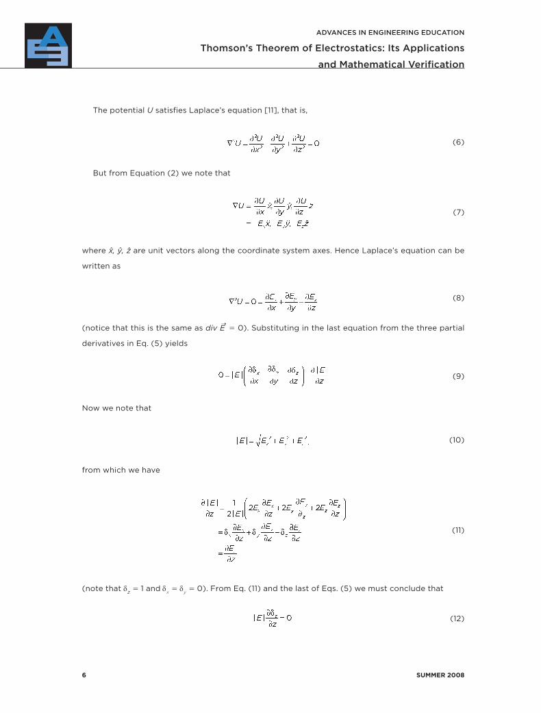
The potential U satisfies Laplace’s equation [11], that is,

(6)

But from Equation (2) we note that

(7)

where x, y, z are unit vectors along the coordinate system axes. Hence Laplace’s equation can be

written as

(8)

(notice that this is the same as div E➝

0). Substituting in the last equation from the three partial

derivatives in Eq. (5) yields

(9)

Now we note that

(10)

from which we have

(11)

(note that δz 1 and δ

x δ

y 0). From Eq. (11) and the last of Eqs. (5) we must conclude that

(12)


SUmmeR 2008 7




And hence ∂δz/∂z 0 (this result, as a matter of fact, should have been an obvious result). Eq. (9)

now reduces to

(13)

The rate of change of a direction cosine, such as δx or δ

y, is related to the concept of “curvature”

of a curve by a well known relationship. This relationship can be derived in a simple manner without

invoking differential geometry, as follows:

In Figure 3, let the arbitrary curve shown be a curve embedded in the surface under consideration

and directed along one of the principal directions. At the specific point where the electric field vector

E➝

is considered, the X axis is tangent to the curve and R is the radius of a circle that is also tangent to

the curve. In theory, if we consider R to be the “radius of curvature” of the curve at the point under

consideration, then the circle is also known as the “osculating” circle. For an infinitesimal deviation

of the vector E➝

from the vertical direction, the cosine of the angle θx can be determined from the

small triangle shown in the Figure. That is, for a small deviation from the vertical, the cosine of the

angle θx, formed between X and the electric field vector E

➝, is approximately equal to x /R, where R

is the radius of the osculating circle that defines the “radius of curvature” of the curve. We have

(14)

Hence,

(15)

Figure 3. An arbitrary curve and its tangent direction, X, at a point under consideration.


8 SUmmeR 2008




The rate of change of the direction cosine with respect to X is therefore equal to the reciprocal

of the radius of curvature along that principal direction. Since we have two principal directions on

the surface, X and Y, then Eq. (13) can be written as follows:

, (16)

where R1 and R

2 are the so called “principal radii” of curvature of the surface at the point under

consideration. This concludes the proof of Thomson’s formula. The reader who is interested in

learning more about the concept of curvature and about differential geometry in general can refer

to ref. [12]. It is to be noted that when the formula is applied to the case of geodesy (the study of

the earth’s equipotential surface), we merely replace the electric field intensity E➝

by the earth’s

acceleration of gravity g➝ . The problem is otherwise mathematically identical.

The proof given in this paper does not exist in the scientific literature, and it is hoped that it will

be a valuable reference for the researchers who are currently using Thomson’s theorem as well as

to the future generations of students.

ReFeReNCeS

[1] J.J. Thomson, footnote on p. 154 of Maxwell’s Treatise On Electricity and Magnetism, (Dover, New York, NY,

1954).

[2] J.D. Jackson, Classical Electrodynamics , (Wiley, New York, NY, 1962), p. 51.

[3] R.C. Pappas, Differential Geometric Solution of a Problem in Electrostatics, SIAM Rev., Volume 28, p. 225, 1986.

[4] R.J. Haywood, M. Renksizbulut, and G.D. Raithby, Transient Deformation of Freely Suspended Liquid Droplets in

Electrostatic Fields, J. of the American Institute of Chemical Engineers, Volume 37, No. 9, p. 1305, 1991.

[5] J.F. Holmes et al., Laser Modulation of LMI Sources, US Patent No. 5015862, 1991.

[6] E. Bakhoum and J.A. Board, Jr., The Geometric Solution of Laplace’s Equation, J. of Computational Physics, Volume

123, p. 274, 1996.

[7] J.A. Carretero-Benignos, Numerical Simulation of a Single Emitter Colloid Thruster in Pure Droplet Cone-Jet Mode,

Ph.D. Thesis, Massachusetts Institute of Technology, Feb. 2005.

[8] J. Zhanga, K. Adamiak, and G.S. Castle, Numerical Modeling of Negative Corona Discharge in Oxygen Under Dif-

ferent Pressures, Journal of Electrostatics, Volume 65, No. 3, p. 174, 2007.

[9] W.H. Smith, Seafloor Tectonic Fabric from Satellite Altimetry, Annual Review of Earth and Planetary Sciences,

Volume 26, p. 697, 1998.

[10] G.A. Estevez and L.B. Bhuiyan, Power Series Expansion Solution to a Classical Problem in Electrostatics, Am. J.

Phys., Volume 53, p. 133, 1985.

[11] W.H. Hayt, Jr. and J.A. Buck, Engineering Electromagnetics, (McGraw-Hill, New York, NY, 2006).





[12] Manfredo P. DoCarmo, Differential Geometry of Curves and Surfaces, (Prentice Hall, Englewood Cliffs, NJ,

1976).

[13] J. Stoer and R. Bulirsch, Introduction to Numerical Analysis, (Springer-Verlag, New York, NY, 1980), p. 96.

AUTHOR

ezzat G. Bakhoum received his Ph.D. degree in electrical engineering from Duke University in

1994. He was a senior engineer at Lockheed Martin and other corporations for six years, and served

as a lecturer in an academic institution for five years. He is now an Assistant Professor of electrical

and computer engineering at the University of West Florida.

Address Correspondence to:

Ezzat G. Bakhoum

Department of Electrical and Computer Engineering

University of West Florida

11000 University Parkway, Pensacola FL 32514

E-mail: [email protected]

SUmmeR 2008 9


10 SUmmeR 2008

APPeNDIX

Here we give the outline of a two-dimensional software algorithm for field mapping based on

Thomson’s theorem. The reader who is interested in obtaining more details about the actual code

should consult [6], as such details are beyond the intended scope of this paper. It is assumed that

both Dirichlet and Neumann boundary conditions are given for the problem under consideration

(if the Neumann boundary conditions are not given, see [6] for details on obtaining such boundary

conditions).

We shall use the simple problem V X2 Y2 of Figure 2(a) as an example to illustrate the field

mapping algorithm. The first step in the algorithm is to determine the points or the equipotentials

on the boundary of the problem where the potential is a local maximum or minimum. In Figure 4, the

local maxima and minima on the boundary are the four points where V 11, 1, 11, 1, as shown.

Our objective now is to determine the equipotential curves V2, V

3, etc., shown in the figure, starting

from any of the indicated four points on the boundary. By using a linearized Taylor series at every

point on the equipotential curve V2, we have

(17)

where V1 11 is the potential at the starting point, and s is the distance along the electric field line

(see figure). But since

(18)

where the potential is decreasing, thus, in Fig. 4,

(19)

Hence, by selecting a suitable voltage V2 (such that the linear approximation holds), and by

knowledge of the magnitude of the electric field intensity, a point can be obtained inside the domain

that lies on the equipotential curve V2. The magnitude of the electric field intensity is assumed to be

known on the boundary and can be calculated from the boundary conditions. It will be given by:

(20)

Now, given one support point on the equipotential curve V2, plus two points on the boundary, a

polynomial of degree 2 can be fitted to represent that equipotential curve (see any standard text


Thomson’s Theorem of electrostatics: its Applications and Mathematical

verification


SUmmeR 2008 11




on numerical analysis, such as [13]). To proceed further inside the domain, we must now obtain the

electric field intensity at 3 points on the equipotential V2 (see Fig. 4) in order to compute a new set

of distances ∆si (V

2 V

3)/E

i , and hence determine the location of the equipotential curve V

3. The

field intensity at the two points on the boundary are known from the boundary conditions. At the point

inside the domain, however, the field intensity can be computed from the linearized approximation

(21)

where |E2| is the magnitude of the field near the equipotential V

2, as shown. The quantity ∂|E

1|/∂s

must now be calculated from Thomson’s formula in two dimensions, that is,

(22)

where 1/R is the reciprocal of the radius of curvature of the equipotential curve V2 at the point inside the

domain. The quantity 1/R is also commonly known as the “curvature” of the curve, and is usually given

the symbol K. Now, if the curve will be mathematically represented by a polynomial of the form y f

(x), then the curvature K can be found from a formula that is well known in numerical analysis [13]:

(23)

where y f(x) and y f (x).

Figure 4. The field mapping.


12 SUmmeR 2008




Having a polynomial representation for the equipotential curve V2, the first and second deriva-

tives of the function y f (x) must then be computed at all the points on the curve that lie inside

the domain (one point, in this example). The most convenient method of interpolation to represent

the function y f (x) under this scheme will be the interpolation by cubic splines [13], since the

method of interpolation by cubic splines features some readily available formulas for computing

the required derivatives.

Tracing additional equipotentials beyond V3 will be carried out by simply repeating the above

steps. We have given hereinabove an outline for a field mapping algorithm that is based on Thomson’s

theorem. More details, including a breakdown of the actual working code, can be found in [6].


Date post:	10-Apr-2018
Category:	Documents
Upload:	vonhu
View:	214 times
Download:	1 times

Advances in engineering educationadvances.asee.org/wp-content/uploads/vol01/issue02/... · ·...

Documents