AECTP 600 THE TEN STEP METHOD FOR EVALUATING THE …

AECTP-600

Edition 2

ALLIED ENVIRONMENTAL CONDITIONS AND TEST PUBLICATION

AECTP 600

THE TEN STEP METHOD FOR EVALUATING THE ABILITY OF MATERIEL TO MEET

EXTENDED LIFE REQUIREMENTS AND ROLE AND DEPLOYMENT CHANGES

Downloaded from http://www.everyspec.com

AECTP-600

Edition 2

INTENTIONALLY BLANK


AECTP-600 (Edition 2)

III ORIGINAL

NORTH ATLANTIC TREATY ORGANIZATION

NATO STANDARDISATION AGENCY (NSA) NATO LETTER OF PROMULGATION April 2007 1. AECTP-600 (Edition 2) – THE TEN STEP METHOD FOR EVALUATING THE ABILITY OF MATERIEL TO MEET EXTENDED LIFE REQUIREMENTS AND ROLE AND DEPLOYMENT CHANGES is a NATO/PFP UNCLASSIFIED publication. It shall be transported, stored and safeguarded in accordance with agreed security regulations for the handling of NATO/PFP UNCLASSIFIED documents. The agreement of nations to use this publication is recorded in STANAG 4370. 2. AECTP-600 (Edition 2) is effective upon receipt. It supersedes AECTP-600 (Edition 1) which shall be destroyed in accordance with the local procedure for the destruction of documents. 3. AECTP-600 (Edition 2) contains only factual information. Changes to these are not subject to the ratification procedures; they will be promulgated on receipt from the nations concerned. 4. It is permissible to reproduce this AECTP in whole or in part provided the same level of security classification is maintained.

J. MAJ Major General, POL(A) Director, NSA


AECTP-600

Edition 2

i

ALLIED ENVIRONMENTAL CONDITIONS AND TEST PUBLICATION

AECTP 600

EXECUTIVE SUMMARY

1. A process known as the Ten Step Method has been developed for evaluating the ability of materiel to meet extended life requirements and role and deployment changes. The process is presented in this AECTP, which is a framework document. The purpose of this document is to acquaint project (program) managers with the engineering principles involved when evaluating the implications of extended life requirements, and also with the outline of a management tool that systematically addresses the issues to be resolved. Additional leaflets are included to provide further guidance for the engineering practitioner when addressing the detailed technical issues.

2. As a management tool, the Ten Step Method provides:

• a structured economical process to aid conformity and traceability when evaluating extended life requirements and role and deployment changes

• an explanation of the necessary steps to be undertaken to achieve compliance with extended life requirements and role and deployment changes

• exit criteria from the process that minimise programme costs and timescales

• a basis for tailoring the process to meet the needs of a particular item of materiel

• a mechanism to expose data voids early within the evaluation

• a code of practice to audit materiel life extension, role and deployment change programmes

3. From the engineering viewpoint, the process demands a definitive knowledge of the project specific environmental requirements, for which characteristics and data are available in STANAG 4370 AECTP 200. The process also demands an extensive knowledge of the relevant potential failure modes for the materiel, which should be well known to the original design authorities. This knowledge will provide maximum confidence in the results of the evaluation.

4. Historically, other approaches have been used to evaluate the life of materiel. However, these approaches have serious inherent limitations, particularly with regard to the level of confidence established for life estimates. One such approach applies the test methods and severities used originally to qualify the materiel with the test durations suitably modified to cover the extended life requirements, without regard to the environmental descriptions associated with real life experience to date or from the failure modes that could arise from changes in anticipated usage.

5. In short, the benefits of adopting the Ten Step Method are:

• uncertainties from materiel life evaluation are minimised because the process requires re-examination of the original environmental conditions, possible failure modes and the previous assumptions

• mismatches between the original requirements and real life experience are revealed, thereby eliminating the need to re-test if over-specified, and showing areas of critical need for re-analysis or re-test

• additional work is limited to that which this process shows to be necessary by reducing the large number of possible failure modes to those that affect the life extension criteria and then further reducing the scope of treatments to the most cost effective combination of tests and analyses


AECTP-600

Edition 2

ii

• the process is responsive to the need to reorganise programme time and cost restraints as it exposes the choices available

6. If the extension involves a role, deployment or a design change, care needs to be taken to ensure that all of the appropriate environmental conditions and possible failure modes are considered.


AECTP-600

Edition 2

iii

THE TEN STEP METHOD FOR EVALUATING THE ABILITY OF MATERIEL TO MEET EXTENDED LIFE REQUIREMENTS AND ROLE AND DEPLOYMENT CHANGES

TABLE OF CONTENTS

Page

EXECUTIVE SUMMARY..................................................................................................................................i

1 SCOPE......................................................................................................................................................1

1.1 Purpose ...............................................................................................................................................1 1.2 Application ...........................................................................................................................................1 1.3 Limitations............................................................................................................................................1

2 RELATED DOCUMENTS..........................................................................................................................1

3 INTRODUCTION TO THE METHOD.........................................................................................................2

4 PROVISIONS AND BENEFITS .................................................................................................................7

5 THE TEN STEPS.......................................................................................................................................8

5.1 Step 1: Research the original Life cycle Environmental Profile ............................................................8 5.2 Step 2: Research life history and prepare LCEP..................................................................................8 5.3 Step 3: Prepare an LCEP for the extended life ....................................................................................9 5.4 Step 4: Compare LCEPs......................................................................................................................9 5.5 Step 5: Evaluate adverse deltas to determine potentially critical cases................................................9 5.6 Step 6: Determine the probable critical cases that require additional treatment .................................10 5.7 Step 7: Formulate treatment options for each probable critical case..................................................11 5.8 Step 8: Select options and compile work programme ........................................................................12 5.9 Step 9: Undertake the planned tasks .................................................................................................13 5.10 Step 10: Evaluate results from the tasks and compile statement .....................................................13

6 CONCLUDING REMARKS .....................................................................................................................13

ANNEX A: A DEMONSTRATION OF THE TEN STEP METHOD .............................................................A-1

ANNEX B: RELATIONSHIP BETWEEN ENVIRONMENTAL CONDITIONS AND ENVIRONMENTAL DESCRIPTIONS FOR TYPICAL LCEP CONDITIONS ...........................B-1

ANNEX C: BIBLIOGRAPHY......................................................................................................................C-1

ANNEX D: GUIDANCE FOR THE ENGINEERING PRACTITIONER........................................................D-1 Leaflet 601 Reverse engineering..............................................................................................D-3 Leaflet 602 Time compression ...............................................................................................D-15 Leaflet 603 Incremental acquisition ........................................................................................D-21 Leaflet 604 Physics of failure..................................................................................................D-29 Leaflet 605 Information requirements for LCEPs (Steps 1 to 3) .............................................D-43 Leaflet 606 Probabilistic analyses .........................................................................................D-49 Leaflet 607 Materiel role and deployment changes ................................................................D-59


AECTP-600

Edition 2

iv

INTENTIONALLY BLANK


AECTP-600

Edition 2

1

THE TEN STEP METHOD FOR EVALUATING THE ABILITY OF MATERIEL TO MEET EXTENDED LIFE REQUIREMENTS AND ROLE AND DEPLOYMENT CHANGES

1 SCOPE

1.1 Purpose

1.1.1 The purpose of this AECTP is to describe the process known as the Ten Step Method that has been developed to determine the ability of materiel to meet extended life requirements and role and deployment changes. The process is presented in this AECTP, which is a framework document. The purpose of the document is to acquaint project (programme) managers with the engineering principles involved when evaluating the implications of extended life requirements, and with the outline of a management tool that systematically addresses the issues to be resolved.

1.1.2 The following Annex D leaflets are intended to provide additional guidance for the engineering practitioner when addressing the detailed technical issues.

601 Reverse Engineering 602 Time Compression 603 Incremental Acquisition 604 Physics of Failure 605 Guidance on Information Required for Steps 2 and 3 606 Probabilistic Analysis 607 Role and Deployment Changes

1.2 Application

1.2.1 The process described in this AECTP is applicable to all materiel projects. It is especially applicable to joint NATO materiel projects and multi-national materiel projects.

1.2.2 The process is comprehensive and ensures that all appropriate environmental conditions, design modifications, possible failure modes and earlier qualification assumptions have been considered. Moreover, streamlining and early exit criteria are integrated systematically into the process to eliminate unnecessary work.

1.3 Limitations

1.3.1 The application of the process is limited to materiel where life is a function of exposure to environmental stresses.

2 RELATED DOCUMENTS

- STANAG 4370 Environmental Testing - AECTP 100 Environmental Guidelines - AECTP 200 Environmental Conditions - AECTP 300 Climatic Environmental Tests - AECTP 400 Mechanical Environmental Tests - AECTP 500 Electrical/Electromagnetic Environmental Tests - STANAG 2895 Extreme Climatic Conditions and Derived Conditions for Use in

Defining Design/Test Criteria for NATO Forces Materiel - STANAG 4315 Life Assessment of Munitions


AECTP-600

Edition 2

2

- Mil-Std-810 Test Method Standard for Environmental Engineering Considerations and Laboratory Tests

- Def Stan 00-35 Environmental Handbook for Defence Materiel - GAM-EG-13 Essais Généraux en Environnement des Matériels - CIN-EG01 Guide pour la prise en compte de l’Environment dans un - Programme d’Armement - CPM 2001 Customer Product Management 2001

3 INTRODUCTION TO THE METHOD

3.1 A premise of the Ten Step Method in general, and Step 1 in particular, is that the materiel under consideration was originally developed and qualified to a recognisable form of environmental engineering control and management process such as that presented in STANAG 4370 and its AECTPs or in equivalent national or commercial standards. The environmental processes defined in these standards have been available only in recent years and consequently applied to a limited number of materiel development programmes. Therefore, most materiel requiring life extension was qualified to standardised test criteria in earlier issues of national standards, such as Mil-Std-810 (prior to revision D), Def Stan 07-55 (predecessor to Def Stan 00-35) and GAM-T-13 (predecessor to GAM-EG-13). However, the Ten Step Method can be applied retrospectively, provided that the original environmental descriptions together with the associated design and test criteria are known. A method to deduce the original Life Cycle Environmental Profile (LCEP) environmental conditions by 'reverse engineering' is given in Annex D Leaflet 601. If the extension involves a role, deployment or design change, care needs to be taken to ensure that all appropriate environmental conditions and possible failure modes are considered (see Steps 4 and 7 and the guidance provided in Annex D Leaflet 607).

3.2 The following paragraphs (3.3 to 3.11) provide a brief introduction to the Ten Step Method. The full description of the method is presented in Paragraph 5. A demonstration of the Ten Step Method can be found in Annex A. The inter-relationship between the ten steps is shown in Figure 1, while the required inputs and the expected outputs for each of the ten steps are shown in Figure 2.

3.3 The purpose of Step 1 is to research the original LCEP, especially its environmental descriptions, to establish the baseline for comparative studies with the output from the actual life history to date (Step 2), and the output from the extended LCEP (Step 3). The relationship assumed between environmental conditions and environmental descriptions for typical LCEP conditions is included as Annex B.

3.4 In Step 2, as much data and information as possible are gathered about the in-service history to date, including how the materiel was used and any failures or problems that have occurred. If the service history does not meet the conditions as defined in the original LCEP then an updated LCEP, including its associated environmental descriptions, is prepared for the in-service history to date.

3.5 The purpose of Step 3 is to prepare an LCEP to cover the extended life and/or role change requirements. It is a prerequisite for Step 3 that a fully defined LCEP is available for the future use of the materiel.

3.6 Step 4 is directed at comparing the original planned in-service environmental descriptions with those actually encountered to date (Step 2), combined with those now needed to meet the extended life requirements for the materiel (Step 3). The purpose of the comparison is to quantify the environmental descriptions so that an assessment can be made as to whether the materiel can withstand the environmental stresses expected during the required extended life. Where extended life requirements, combined with those actually encountered, produce more severe environmental descriptions than those to which the materiel was qualified, then the more severe environmental descriptions are known as ‘adverse deltas’. The results of the comparison may demonstrate that there are no adverse deltas and therefore the materiel is already qualified


AECTP-600

Edition 2

3

to withstand the environmental stresses expected during the required extended life. Consequently, the requirements for Exit Criterion 1 are met, Steps 5 through 9 are deleted and Step 10 is used to document the results (see Figure 1). When the extension involves a design change to enhance materiel performance, all environmental conditions should initially be considered as deltas. Engineering judgement is then required to determine whether these deltas can be eliminated or considered as adverse deltas.

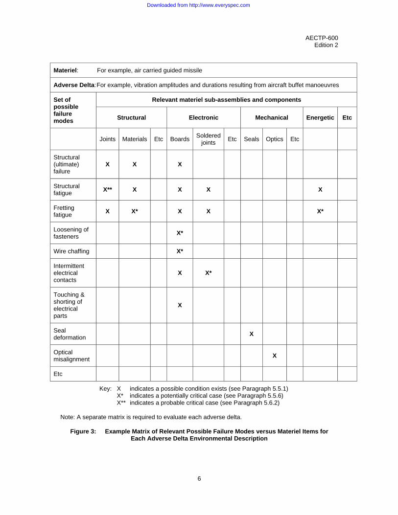
3.7 At Step 5, the Ten Step Method addresses failure modes. The process requires consideration of the possible failure modes that could occur on exposure to the environmental conditions identified as adverse deltas. Therefore, the initial task in Step 5 is to list, for each adverse delta, sets of possible failure modes for sub-assemblies and components. A simplified example of the outcome of this task is shown as a matrix in Figure 3, where the X elements depict the sets of relevant possible failure modes for the sub-assemblies and components. Next, for each identified adverse delta, the sensitivity of the materiel to the sets of relevant possible failure modes is qualitatively assessed to identify potential critical cases (X* in Figure 3), where the extended life environmental requirements may not be met without further treatment, or may even demand design modifications.

3.8 At Step 6, the potential critical cases are quantitatively evaluated for each adverse delta environmental description and the probable critical cases are identified. The sensitivity of the materiel to the original life requirement should be available in terms of analysis or test results, but if not, then it needs to be determined. Similarly, for adverse deltas for which possible failure modes have not been identified, data from additional analyses or tests may be required to detect them. If the results of these evaluations indicate that the estimated life of the materiel, based on the original environmental descriptions, is greater than the estimated life based on the actual and extended life and/or role change requirements, then no further action is required. In such cases the requirements for Exit Criterion 2 are met, Steps 7 through 9 are deleted and Step 10 is used to document the results (see Figure 1).

3.9 Further treatment is necessary where the results from the Step 6 evaluations indicate that the estimated life of the materiel, based on the original environmental descriptions, is less than the actual demonstrated in-service life based on actual history, plus the extended life and/or role change requirements. These probable critical cases are identified as X** in Figure 3. Step 7 indicates how to compile effective treatment options to meet the shortfall for a particular probable critical case.

3.10 At Step 8, the most cost and programme effective treatment options are selected to address all the shortfalls arising from all the adverse deltas and associated probable critical cases. It is intended that these treatments will verify (to an appropriate level of confidence) that the materiel will meet the extended life requirements and role and deployment changes.

3.11 The additional treatments necessary to provide the evidence for the extended life and/or role change requirements, such as analyses, testing and assessments are undertaken at Step 9. At Step 10, the activities to prepare the formal statement on life extension, role and deployment changes are addressed.


AECTP 600 Edition 2

4

Error! Objects cannot be created from editing field codes.

Figure 1: Inter-Relationship between the Ten Steps


AECTP-600

Edition 2

5

Step Action Input information Output information

1. Research the original LCEP (LCEP-1)

Platform(s) used Mission profiles Environmental design/test criteria Analysis/test reports

LCEP-1 or synthesised original LCEP containing environmental descriptions

2. Research subsequent life history, testing, modifications, upgrades

Actual scenarios Surveillance testing Design modifications Re-testing

Materiel LCEP (LCEP-2) to date, design changes and weaknesses

3. Prepare ‘extended life’ and/or role change LCEP (LCEP-3)

‘Extended life’ requirement(s) Geographical location(s) Platform(s) used and any role or deployment changes

‘Extended life’ and/or role change LCEP-3

4. Compare original LCEP-1 environmental descriptions with those for life history to date (LCEP-2) plus those for extended life and/or role change (LCEP-3)

Step 1, Step 2 and Step 3 outputs Statement of the differences in environmental descriptions (deltas). Is Exit Criterion 1 met?

5. Evaluate LCEP differences to determine potentially critical cases for each ‘adverse delta’

Knowledge of failure modes and of materiel properties for the materiel, also for any design modifications

Potentially critical cases for evaluation

6. Evaluate the potential critical cases and determine which are the probable critical cases that require treatment

Compliance statements and hazard analyses, and associated analysis and test reports

Probable critical cases requiring additional treatment. Is Exit Criterion 2 met?

7. Formulate treatment options for each probable critical case

Analysis techniques and testing options

Sets of treatment options for each probable critical case

8. Select cost effective treatment and compile work programme

Cost and programme constraints Work programme and resources required

9. Undertake the planned tasks

Work programme and resources Life assessment information

10. Evaluate results and compile life extension statement

Results of the work programme Statement on life extension and/or role change

Figure 2: Inputs and Outputs for Each of the Ten Steps


AECTP-600

Edition 2

6

Materiel: For example, air carried guided missile

Adverse Delta: For example, vibration amplitudes and durations resulting from aircraft buffet manoeuvres

Relevant materiel sub-assemblies and components Set of possible failure modes Structural Electronic Mechanical Energetic Etc

Joints Materials Etc Boards Soldered joints Etc Seals Optics Etc

Structural (ultimate) failure

X X

X

Structural fatigue X** X X X X

Fretting fatigue X X* X X X*

Loosening of fasteners

X*

Wire chaffing X*

Intermittent electrical contacts

X X*

Touching & shorting of electrical parts

X

Seal deformation

X

Optical misalignment

X

Etc

Key: X indicates a possible condition exists (see Paragraph 5.5.1) X* indicates a potentially critical case (see Paragraph 5.5.6) X** indicates a probable critical case (see Paragraph 5.6.2)

Note: A separate matrix is required to evaluate each adverse delta.

Figure 3: Example Matrix of Relevant Possible Failure Modes versus Materiel Items for Each Adverse Delta Environmental Description


AECTP-600

Edition 2

7

4 PROVISIONS AND BENEFITS

4.1 As a management tool, the Ten Step Method provides:

• a structured economical process to aid conformity and traceability when evaluating extended life requirements and role and deployment changes

• an explanation of the necessary steps to be undertaken to achieve compliance with the extended life requirements and role and deployment changes

• exit criteria from the process that minimise programme costs and timescales

• a basis for tailoring the process to meet the needs of a particular item of materiel

• a mechanism to expose data voids early within the evaluation

• a code of practice to audit completed materiel life extension, role and deployment change programmes

4.2 From the engineering viewpoint, the Ten Step Method demands a definitive knowledge of the project specific environmental requirements, for which characteristics and data are available in STANAG 4370 AECTP 200. To provide maximum confidence in the results of the evaluation, the process requires an extensive knowledge of the relevant potential failure modes for the materiel. Moreover, it is only possible to have confidence in the results of the evaluation if staff with the appropriate knowledge and training are involved in the process.

4.3 Historically, other approaches have been used to evaluate the life extension of materiel. However, these approaches have serious inherent limitations, particularly with regard to the level of confidence established for life estimates. One approach applies the original test methods and severities used to qualify the materiel, with only the test durations modified to cover the extended life requirements. This approach does not consider the environmental descriptions associated with real life experience to date or of the failure modes that could arise from changes in anticipated usage.

4.4 In short, the benefits of adopting the Ten Step Method are:

• uncertainties from the life extension evaluation are minimised because the process requires re-examination of the original environmental descriptions, potential failure modes and the previous assumptions.

• mismatches between the original requirements and in-service experience are revealed, identifying only areas of critical need for re-analysis or re-test.

• additional work is limited by reducing the large number of possible failure modes to those that affect the life extension criteria. The scope of treatments is then further reduced to the most cost effective combination of tests and analyses.

• early exit criteria allow a conclusion to be reached based upon a minimum number of steps eliminating the need to complete the remaining ten steps. These criteria take into account cost and risks.

• the process is responsive to the need to reorganise the programme time and cost restraints as it exposes the choices available.


AECTP-600

Edition 2

8

5 THE TEN STEPS

5.1 Step 1: Research the original Life Cycle Environmental Profile

5.1.1 Obtain the Manufacture to Target or Disposal Sequence (MTDS) and associated environmental descriptions which are often contained in an Environmental Requirement document. For the purpose of this AECTP it is assumed that the MTDS and environmental descriptions are contained in one document called the Life Cycle Environmental Profile (LCEP). Therefore, an LCEP is expected to consist of logistic and operational scenarios together with their associated environmental descriptions, which should include:

• Handling, transportation and storage

• Deployment platform (ie: truck, aeroplane, ship etc)

• Mission profile/service use profile

• Disposal

5.1.2 The original LCEP forms the baseline document for the Ten Step Method for evaluating the ability of materiel to meet extended life requirements. If the LCEP information is not available, then environmental descriptions will need to be synthesised from the following project specific documentation:

• Environmental Design Criteria

• Environmental Test Specification

• Analysis and Evaluation Reports

• Test and Assessment Reports

A method to deduce the original LCEP environmental conditions by 'reverse engineering' is given in Leaflet 601 of Annex D.

5.2 Step 2: Research life history and prepare LCEP

5.2.1 Obtain information concerning any modifications to the materiel or changes to its original intended usage. Investigate any additional testing performed subsequent to placing the materiel in service. This information should include the following:

• A profile of the in-service life in terms of batch/lot, design standard, age and deployment

• Results from materiel integrity and safety analyses and assessments

• Results from surveillance inspections and testing

• Recalls to fix problems, the causes of such problems, and the results of any related analyses and tests

• Design upgrades, the issues that prompted them, and the results of any related analyses and tests

• Manufacturing process changes

5.2.2 Care needs to be taken when gathering this information since the materiel in the inventory may represent several production runs produced over several years by different suppliers. The inventory may consist of pieces of materiel which are the same as originally built, or retrofitted, eg: line replacement items, or a mixture of original materiel and improved materiel.

5.2.3 For ease of comparison in Step 4 below, an updated LCEP, including its associated environmental descriptions should be prepared for the in-service history to date.


AECTP-600

Edition 2

9

5.3 Step 3: Prepare an LCEP for the extended life requirement

5.3.1 Prepare an LCEP covering the extended life and/or role change requirements based on current knowledge and understanding of in-service usage. It can be expected that, since the materiel was designed, the deployment platforms will have changed as well as the geographical locations for deployment, and perhaps the performance expected from the materiel. Each of these will affect, and may increase, the environmental stress levels.

5.3.2 As part of the content of the extended life LCEP, compile a set of environmental descriptions that represent the conditions expected during in-service usage for the required extended lifetime. If the extension involves a role or deployment change, or a design change, care needs to be taken to ensure that all of the appropriate environmental conditions and possible failure modes are considered (see the guidance provided in Leaflet 607 of Annex D).

5.3.3 Where improved data is now available, it is possible that the environmental descriptions for a particular in-service LCEP are at variance with those stated in the original LCEP, even though the requirement for those LCEP conditions remains unchanged. In such cases, the improved data in the LCEP for the extended life should be included and the consequences in Step 4 evaluated.

5.4 Step 4: Compare LCEPs

5.4.1 For each environmental description in the original and extended life LCEP documents, compare the original severities (Step 1) with those for the extended life requirements (Step 3) combined with those for the actual life history completed to date (Step 2). Care should be taken to present the differences, colloquially known as ‘deltas’, in a common format for ease and accuracy of comparison with related environmental descriptions. Refer to Annex D Leaflets 601 and 602 for guidance when performing this step. Check whether the original environmental descriptions and failure modes and associated acceptance criteria remain valid. When the extension involves a design change to enhance materiel performance, all environmental conditions should be initially considered as adverse deltas. Engineering judgement is then required to determine whether or not they can be eliminated.

5.4.2 As stated in Step 1, if the original levels were not based on an LCEP, but rather on standardised tests, then an equivalent original LCEP will need to be developed comprising synthesised environmental descriptions as necessary.

5.4.3 Recommended practices should be followed where time compression, or perhaps decompression, techniques are needed to aid comparison of levels. Refer to Annex C for a bibliography of life evaluation and test time compression documents (see Annex D Leaflet 602). Record when these techniques are used for such comparisons.

5.4.4 It may be possible to demonstrate that the original LCEP generated design and test severities represent cumulative stresses which are greater than expected during the lifetime completed to date, plus those expected during the extended life. Where this is so, and where no design modifications are proposed, a case can be made for recommending the required extended usage without further detailed investigation, analysis or testing. Should this demonstration be successful, no additional work is necessary and the requirements for Exit Criterion 1 are met, Steps 5 through 9 are deleted, and Step 10 is used to document the results (see Figure 1).

5.5 Step 5: Evaluate adverse deltas to determine potentially critical cases

5.5.1 In this step the failure modes of the materiel and of any proposed design modifications are addressed. The process requires the consideration of potential failure modes that could occur on exposure to the adverse delta environmental stresses. Therefore the initial task in this step is to list sets of possible failure modes of subassemblies and components for each adverse delta.


AECTP-600

Edition 2

10

5.5.2 This initial task is achieved by setting up a matrix for each identified adverse delta as shown in Figure 3. The rows in the matrix comprise sets of possible failure modes for the materiel and the columns represent the relevant materiel sub-assemblies and components considered to be sensitive to the adverse delta. Relevant possible failure modes for a specific sub-assembly or component are shown as X elements in Figure 3. A demonstration of the use of the matrix in the Ten Step process is shown in Annex A.

5.5.3 It is intended that the list of possible failure modes includes those which are unique to the materials and processes used in the manufacture of the materiel as well as those which experience has shown will be produced by generic environmental stresses. A bibliography is provided in Annex C to assist with the identification and processing of failure modes.

5.5.4 Extend the list of possible failure modes, as appropriate, to include situations where the original data, evaluations or assumptions, are now considered to be suspect.

5.5.5 Mission criticality tends to fall into the following three categories:

• System performance

• System safety

• Structural integrity

Matrices should be produced as necessary to accommodate all three categories. Determining criticality is based on answering the specific question under consideration, eg: will the materiel be safe to use for the required extended period, or will the materiel perform as required for the same extended period? These are separate questions and each needs to be addressed using separate criteria.

5.5.6 For each adverse environmental condition, the size of the matrix of possible failure modes versus materiel sub-assemblies and components should be reduced as much as possible. This may be achieved by conducting a review to ascertain whether each listed possible failure mode will generate a potentially critical case. A potentially critical case (depicted as an X* element in Figure 3) is defined as a case which affects mission requirements. The review will be qualitative and subjective at this stage and based mainly on experience. This experience should include knowledge of the physics of failure for the materials from which the materiel is made, and previous knowledge of this or similar materiel.

5.5.7 Further consideration only needs to be given to the matrix elements representing failure modes that could generate potentially critical cases. The nature of the potentially critical cases should be recorded. (An example of a reduced matrix in tabular form and recorded potentially critical cases is given in Annex A Figure A1 Columns 4 and 5.)

5.5.8 It is emphasised that the overall confidence in the results of the total life estimation task is directly related to the diligence employed when completing Step 5.

5.6 Step 6: Determine the probable critical cases that require additional treatment

5.6.1 The purpose of this step is to evaluate quantitatively the criticality of each identified potentially critical case so that an informed decision can be made as to whether additional treatment is required, or whether the original (or current) qualification is acceptable. The combination of assessments, analyses and/or testing is commonly referred to as ‘treatment’ in this document. Prior to making this decision, all relevant data sources available should be reviewed. With regard to the three mission categories referred to in Step 5, these sources could include:

• Materiel performance specifications to ascertain mission critical and minimum performance requirements


AECTP-600

Edition 2

11

• Project hazard analyses to ascertain the consequences of failure(s) resulting in a potentially unsafe condition

• Project compliance matrices which, for structural integrity requirements, would include references to relevant structural strength summaries, structural assessment reports, stress analyses and strength test reports

5.6.2 An assessment should be made as to which of the potentially critical cases need to be considered further. Those to be considered further are termed ‘probable critical cases’ (depicted as an X** element in Figure 3).

5.6.3 The probable critical cases that require additional treatment and the reasons for the additional treatment should be recorded.

5.6.4 A demonstration of how the critical cases can be processed through Step 6, from potential to probable, is given in Annex A Figure A2.

5.6.5 Should the results of the evaluation indicate that none of the potentially critical cases arising from the extended life and/or the role change requirements need additional treatment, and the original (or current) qualification is acceptable, no additional work is necessary and the requirements for Exit Criterion 2 are met, Steps 7 through 9 are deleted, and Step 10 is used to document the results (see Figure 1).

5.7 Step 7: Formulate treatment options for each probable critical case

5.7.1 At this point:

• all LCEP environmental conditions have been reduced to only the adverse deltas (Step 4);

• the matrices for each adverse delta listing possible failure modes of the original materiel and any design modifications have been reduced to only the potential critical cases (Step 5); and

• all associated project specific data have been evaluated to determine probable critical cases that require additional treatment to meet the extended life requirements (Step 6).

The purpose of Step 7 is to formulate treatment options for each remaining probable critical case. The treatment options could include the following:

• Sophisticated analysis/modelling and/or evaluation without testing, eg: finite element analysis with supporting technical documentation

• Analysis supported by characterisation testing, eg: modal analysis testing

• Tailored sequential environmental testing (natural or laboratory) supported by technical validation

• Minimum integrity environmental testing supported by an evaluation report to justify the validity of the testing

• Additional surveillance

5.7.2 If it is considered, based on the assessments in Steps 5 and 6, that an adverse delta is so severe that the materiel cannot possibly meet the extended life requirement, or that a sophisticated treatment is not cost effective, then it may be feasible to modify the planned usage of the materiel to alleviate the environmental condition such that the adverse delta is reduced or eliminated. Alternatively, stress mitigation measures or design changes can be incorporated, followed by re-qualification of the materiel as appropriate. Such recommendations should be documented in Step 10.


AECTP-600

Edition 2

12

5.7.3 Options involving analysis methods will need to consider the full range of techniques currently available in order to achieve the most effective solution.

5.7.4 Options involving testing will need to consider whether to test at system, sub-assembly or coupon level in order to achieve the most effective solution. STANAG 4370 AECTP 200 provides guidance on the selection of environmental tests, while in AECTPs 300, 400 and 500 a full range of both tailored and minimum integrity test methods is defined.

5.7.5 Where a relatively high level of confidence is required, consideration should be given to the merits of adopting the ‘multi-legged’ assessment approach (see Annex C Section 1 References 2 and 29). This approach is defined as a combination of analysis, modelling, testing and assessment methodologies to provide the case for materiel qualification at the required confidence level. The degree to which each methodology is used will be based on a trade-off between time, cost and required confidence.

5.7.6 A short list of the preferred treatment options for each probable critical case should be recorded together with a justification for the option chosen.

5.8 Step 8: Select options and compile work programme

5.8.1 In this step the treatment options derived in Step 7 for each probable critical case are reviewed, and the most effective approach to accommodate all the treatments in an appropriate sequence is evaluated. It may be possible to address some of the effects of environmental conditions by modelling, eg: certain structural dynamic loadings, but others will require testing, eg: solar radiation. If the treatment options derived in Step 7 are heavily analysis orientated, review the possibility of deleting most or all testing tasks. If the treatment options are orientated towards testing, review the need for pre-stressing, ie: additional tests may need to be added into the sequence to generate wear, particularly if the test specimen is relatively unused.

5.8.2 Options involving environmental testing should invoke only accepted environmental test engineering practices, using the guidance provided in the AECTPs covered by STANAG 4370. The following activities need to be addressed when considering testing solutions:

• Determine which environmental stresses can be combined. Advice is given in AECTP 200 Category 240 Leaflet 2410

• Determine the minimum acceptable sample size

• Determine the build standard of the test specimens to be extracted from service use, paying careful attention to the age and previous usage of the materiel

• Tailor test severities using, if necessary, accepted credible time compression techniques; the bibliography presented in Annex C of this document could be used as a guide

• Define fixturing and facility requirements

• Define test configurations

5.8.3 If the results from these additional treatments are likely to be phased with time, then the ‘multi-legged’ approach referred to in Step 7 may be essential to provide the necessary progressive build up of confidence.

5.8.4 A work programme to implement the selected treatments should be compiled. This should include a justification of the approach used and the severities of any test.


AECTP-600

Edition 2

13

5.9 Step 9: Undertake the planned tasks

5.9.1 The purpose of this step is to undertake the planned tasks associated with the selected treatments. The resulting evidence provides the necessary information to determine whether the extended life and/or role change requirements can be met.

5.9.2 The results of the selected treatments should be reported, making sure that the necessary information is available for the Step 10 evaluation.

5.10 Step 10: Evaluate results from the tasks and compile statement

5.10.1 Using the results obtained from Step 9 evaluate the materiel against the extended life requirements and role and deployment changes. This evaluation is likely to include the following activities:

• Assess the ability of the materiel to meet the extended life requirements and/or role and deployment changes, preferably expressed in terms of confidence levels and supported by a risk assessment where appropriate

• Compile requirements for any associated in-service surveillance activities

• Compile recommendations, where relevant, for stress mitigation measures which could include platform limitations and/or restrictions on environmental conditions

• Recommend product improvements, where relevant, to eliminate the need for stress mitigation measures and to meet the requirements in full

5.10.2 Prepare a written statement (report) for approval by the appropriate authority, providing specific information of the changes to the approved life of the materiel and stating all limitations on, or modifications to, the in-service usage.

6 CONCLUDING REMARKS

6.1 This AECTP presents a structured and economical process on which service life extension programmes, and/or role and deployment change programmes can be based. The methodical re-examination of the original LCEP environmental descriptions, potential failure modes, and previous assumptions in relation to extended life requirements minimise the uncertainties present in life extension work. The entire process needs to be thoroughly documented but the accuracy and success of this process relies on the engineers involved having programme, environmental analysis, testing and assessment experience.


AECTP-600

Edition 2

14

INTENTIONALLY BLANK


AECTP-600

Edition 2 ANNEX A

A-1

ANNEX A

A DEMONSTRATION OF THE TEN STEP METHOD

1 INTRODUCTION

1.1 The purpose of this annex is to provide a demonstration of the Ten Step Method. This demonstration provides one example of a methodology for dealing with the complex process of reducing the large number of possible failure modes down to the minimum number required to meet the life extension criteria. The demonstration is based on a question of current interest to many program managers; ‘is it possible to extend the life of the materiel from its current planned life to the required extended life?’

1.2 For this demonstration an air carried guided weapon has been chosen. As discussed in the main document, when considering the life extension for such materiel, there are many environmental issues that can be studied. In this demonstration the life extension requirements are limited to extending the number of flight carriage hours. It is also understood that mission criticality falls into several categories (see Paragraph 5.5.5 in the main document), however this demonstration is further limited to the mission criticality category ‘structural integrity’ only. Safety and performance categories can be covered in a similar manner.

1.3 To simplify the demonstration, the content of this annex is limited to providing additional guidance on the relatively complicated activity of the determination of the probable critical cases and the derivation of their additional treatments, ie: Steps 5, 6 and 7. The demonstration makes simplifying assumptions regarding Steps 1 through 4 and Steps 8 through 10. In actual tasks, other requirements are often addressed concurrently, such as the incorporation of materiel role and deployment changes which need to be addressed in a similar manner (see Annex D Leaflet 607).

1.4 For this demonstration, the steps of the Ten Step Method have been divided into four groups:

• Adverse deltas (Steps 1-4)

• Critical cases (Steps 5-6)

• Treatments (Steps 7-8)

• Compliance (Steps 9-10)

2 ADVERSE DELTAS

2.1 The aim of Steps 1 to 4, as described in Paragraphs 5.1 through 5.4 of the main document, is to identify and quantify the adverse delta environmental descriptions associated with air carried guided weapon extended life requirements. Adverse deltas are defined as any changes in environmental descriptions resulting from the LCEP which extend either the duration or amplitude of the environmental descriptions, or both. A description of the relationship between environmental conditions and environmental descriptions for typical LCEP conditions is included in Annex B.

2.2 It is assumed for this demonstration that Steps 1 to 4 have been completed in accordance with the guidance given in the main document, and that many environmental conditions with increased severity (adverse deltas) have been identified. These adverse deltas may include environmental descriptions relating to extended storage duration, increased operational temperatures, additional handling shocks and increased buffet manoeuvre vibration. However, this demonstration will only address one adverse delta, ie: that of missile buffet manoeuvre vibration, and in particular the effect of increased duration arising from the extended life requirements. For slender air carried missiles this vibration environment arises from


AECTP-600

Edition 2 ANNEX A

A-2

aerodynamic excitation of the missile (or aircraft pylon or wing) during aircraft flight manoeuvre conditions. The missile responses are often characterised by narrow band random vibration and emanate from the excitation of the missile in its fundamental bending mode. This vibration environment can significantly affect the missile’s air carriage fatigue life.

3 CRITICAL CASES

3.1 The aim of Steps 5 and 6, as described in Paragraphs 5.5 and 5.6 of the main document is to determine the critical cases and to establish whether additional treatment, in terms of assessment, analysis and/or testing, is required to demonstrate that the materiel is compliant with the extended life requirements.

3.2 Evaluate adverse deltas to determine potentially critical cases (Step 5)

3.2.1 The purpose of Step 5 is to determine the possible failure modes that could generate potentially critical cases for each of the adverse environmental descriptions (deltas) derived in Steps 1 through 4. As the list of adverse deltas could be extensive for an air carried guided weapon, this task is facilitated by the use of a matrix to evaluate each adverse delta, ie: one matrix for each adverse delta.

3.2.2 A typical matrix format to cover vibration resulting from aircraft buffet manoeuvres (the only adverse delta addressed in this demonstration) is shown in Figure 3 of the main document. Relevant sub-assemblies and components of a typical air carried guided missile are shown listed in the horizontal axis. The relevant possible failure modes for the missile are shown in the vertical axis.

3.2.3 The elements of the matrix in Figure 3 in the 'Structure - Joints' column adjacent to the set of possible failure modes associated with structural failure and fatigue are shown expanded and in tabular format in Figure A1. Shock and impact failure modes have been added. The table demonstrates the processing of each possible failure mode, ie: each populated element in the matrix, within Step 5. Columns 1 and 2 of Figure A1 portray the possible mechanical failure modes of the missile joint structure. In normal circumstances, possible failure modes for climatic, chemical, biological and electrical will also need to be addressed.

3.2.4 For this demonstration, only structural integrity is addressed (see Paragraph 1.2). However, in the general case for air carried guided missiles, the matrix will need to be developed to include elements covering the following categories of mission criticality:

• System performance: functional and reliability

• System safety

• Structural integrity: especially air worthiness

This development infers three separate matrices. Because only structural integrity is addressed, the detailed matrix shown in Figure A1 is formulated to address only airworthiness requirements. Also, to illustrate the flexibility of the Ten Step Method, the matrix content focuses on analytical approaches, but the solutions would of course default to test treatments during subsequent steps if cost effective analytical techniques were unavailable.

3.2.5 When initially completed, the matrix will contain more possible failure modes than would be practical or economical to consider. At this point the possible failure modes for the missile tubular joint structure, as listed in Column 2 of Figure A1, are reviewed against the captive flight buffet manoeuvre vibration (the adverse delta) to determine which of the possible failure modes are relevant to the missile tubular joint under consideration. The list of possible failure modes is likely to be reduced considerably as a result of this exercise, as indicated in Column 3 of Figure A1.


AECTP-600

Edition 2 ANNEX A

A-3

3.2.6 The next task is to review each of the relevant possible failure modes in Column 2 to determine which modes are likely to generate potential critical cases, ie: those that would be potentially critical to the structural integrity of the materiel. The result of this task is indicated in Column 4 as a Yes/No answer. This is complemented in Column 5 with a short narrative summarising the nature of the potentially critical case, how the case is covered, or why the case is not an issue. The review to determine potentially critical cases is subjective at this stage and based mainly on experience. This experience can be based on knowledge of the physics of failure of the material from which the materiel is made, or from experience with similar materiel. An affirmative response in Column 4 of Figure A1 denotes a commitment to carry through this case to Step 6 where its criticality will be quantified.

3.2.7 The overall confidence in the results of the life estimation task will be directly dependent on the diligence with which the matrix is addressed and completed.

Note: The processing of the large number of elements in the matrix for a complex materiel system such as an air carried guided missile would be simplified by the adoption of computer software to automate the identification of possible failure modes, and the subsequent processing to determine potentially critical cases and subsequently probable critical cases (Steps 5 and 6).

3.3 Determine the probable critical cases that require additional treatment (Step 6)

3.3.1 The purpose of this step is to evaluate each potentially critical case so that an informed decision can be made as to whether additional treatment is required, or whether the original (or current) qualification is acceptable. Prior to making this decision, check all relevant data sources available for this adverse delta. These would include project compliance matrices relating to structural integrity requirements, which should indicate references to relevant structural strength summaries and appropriate structural assessment reports, stress analyses and strength test reports.

3.3.2 Conduct the evaluation necessary to make a decision as to which of the potentially critical cases require additional analysis and/or test treatments. The evaluation process for each remaining possible failure mode (ie: each remaining populated element in the Figure 3 matrix) is demonstrated through the use of the table in Figure A2. Columns 6, 7 and 8 of this table essentially summarise the results of Step 5. The required evaluation for each remaining possible failure mode and its associated potential critical case is indicated in Column 9. The evaluation may involve a theoretical or trials analysis, such as re-visiting stress calculations or test reports and their associated assessments.

3.3.3 Considering the air carried guided missile example and Figure A2, analytical and/or test treatments are needed only to cover missile joint structural fatigue modes (see Column 10). The associated potential critical case is then referred to in Column 11 as a probable critical case.

3.3.4 The reasons for the additional treatment should be formally recorded in an appropriate report, summarised in Column 11, together with the reasons why no further work is considered necessary for the eliminated potential critical cases.

3.3.5 Had the evaluation concluded that no further treatment is needed to meet the extended life requirements, ie: Column 10 of Figure A2 had only negative responses, then the requirements for Exit Criterion 2 are met, Steps 7 through 9 are deleted, and Step 10 is used to document the results (see Figure 1 in the main document).

4 TREATMENTS

4.1 The aim of Steps 7 and 8 is to formulate, optimise and programme the treatments required to service the probable critical cases.


AECTP-600

Edition 2 ANNEX A

A-4

4.2 Formulate treatment options for each probable critical case (Step 7)

4.2.1 The purpose of Step 7 is to formulate treatment options for each remaining probable critical case which will confirm, or otherwise, that the materiel is capable of meeting the extended life requirements. The only probable critical case in this air carried guided missile demonstration is that for missile tubular joint fatigue. The following generalised approach for selecting treatment options should be considered:

• Analysis/assessment only

• Analysis supported by characterisation (eg: modal or stiffness) testing

• Tailored environmental testing supported by a minor assessment

• Minimum integrity environmental testing supported by a major assessment

4.2.2 Options involving analysis methods will need to consider the full range of techniques currently available in order to achieve the most cost-effective solution.

4.2.3 Options involving testing will need to consider whether to test at guided missile system level, sub-assembly level, or lower, to achieve the most effective solution. The selection of environmental tests is addressed in AECTP 200, while a full range of both tailored and minimum integrity test methods is defined in AECTP 400.

4.2.4 Where a relatively high level of confidence is required, as in this demonstration, consideration should be given to the merits of adopting the 'multi-legged' assessment approach. This approach is defined as a combination of analysis, modelling, testing and assessment methodologies to provide the case for materiel qualification at the required confidence level. The degree to which each technique is used will be based on a trade off between time, cost and the level of confidence required.

4.2.5 Typically, the process for setting up analysis treatment options for this particular probable critical case is as follows:

(a) Confirm the full details of the adverse delta in terms of the credible worst case, or limit, combination of concurrent load inputs and environmental conditions, eg: the full details could comprise:

• A set of missile buffet conditions that include both store rigid and flexible body motions (the basis of the adverse delta)

• A set of aircraft flight manoeuvres (inducing missile accelerations) acting concurrently

• An associated set of aerodynamic loadings acting concurrently

• Aero elastic effects acting concurrently (where relevant)

(b) Confirm, assisted by the knowledge from (a), the potentially critical areas of the structural joint when subjected to fatigue loadings, eg: critical areas could arise in:

• Joint materials

• Structural discontinuities (stress raisers)

• Fasteners

(c) With the knowledge of (a) and (b), confirm the set of detailed fatigue failure modes that could arise within the missile structural joint.


AECTP-600

Edition 2 ANNEX A

A-5

(d) From (a), (b) and (c) identify relevant fatigue analysis techniques that could confirm whether or not the missile structural joint would meet the extended life requirements. Such techniques could include:

• Fracture mechanics methods

• Cumulative damage methods

• Use of specialist data sheets

• Use of acknowledged codes of practice

(e) In parallel with (d), define specific acceptance criteria for each fatigue failure mode.

Specialist knowledge of fatigue failure modes and the associated physics of failure are required to produce satisfactory results from the above sequence.

4.2.6 For the missile structural joint example, the analysis techniques contained in AECTP 200 Leaflet 2410 - Validation of mechanical environmental test methods and severities - may be helpful when comparing the benefits of relevant treatment options.

4.2.7 Record the list of preferred treatment options for this particular probable critical case.

4.3 Select options and compile work programme (Step 8)

4.3.1 The purpose of Step 8 is to review the treatment options derived in Step 7 for the particular probable critical case, together with those for all the other probable critical cases. (In this example the Step 8 review cannot be done because no other probable critical cases were developed.)

4.3.2 For this air carried guided missile demonstration the remainder of Step 8 would be conducted using the information given under the Step 8 heading in the main document.

5 COMPLIANCE

5.1 The aim of Steps 9 and 10 is to derive and report the evidence that the air carried guided missile complies with the extended life requirements.

5.2 Upon completion of Step 8, for this air carried guided missile demonstration, Steps 9 and 10 would be conducted using the information given under the Step 9 and Step 10 headings in the main document.


AECTP-600

Edition 2 ANNEX A

A-6

INTENTIONALLY BLANK


AECTP 600

Edition 2 ANNEX A

A-7

POTENTIALLY CRITICAL CASES Materiel: Air carriage guided missile Adverse delta: Vibration resulting from aircraft buffet manoeuvres Sub-assembly: Structure - missile tubular joint

1: Sets of possible failure modes

2: Detailed sets of possible failure modes

3: Is this failure mode relevant to the joint?

4: Is this possible failure mode likely to generate a potentially critical case?

5: Record the nature of the potentially critical case

Structural (ultimate) failure Tension Compression Bending Shear Bearing Buckling (general) Buckling (local)

Yes Yes Yes Yes Yes No Yes

No No Yes Yes Yes N/A Yes

Covered by bending Covered by bending Bending stresses of the tube at the joint Shear of the joint fasteners Fasteners in tube material Not applicable Tube between fasteners

Structural fatigue Structural member fatiguePanel fatigue Joint fatigue

Yes No Yes

No N/A Yes

Covered by joint fatigue Not applicable Fatigue of tube (or fasteners)

Fretting fatigue Fretting fatigue Yes No Covered by joint fatigue

Shock and Impact Brittle fracture Strain rate effects Induced impacts

No No Yes

N/A N/A Yes

Not applicable Not applicable Induced displacements

Other

Brinelling Wear Erosion

No No No

N/A N/A N/A

Not applicable Not applicable Not applicable

Note: A ‘Yes’ in Column 3 = X in Figure 3 of the main document A ‘Yes‘ in Column 4 = X* in Figure 3 of the main document

Figure A1: Determine Potentially Critical Cases for Each Adverse Delta (Step 5)


AECTP 600

Edition 2 ANNEX A

A-8

PROBABLE CRITICAL CASES Materiel: Air carriage guided missile Adverse delta: Vibration resulting from aircraft buffet manoeuvres Sub-assembly: Structure - missile tubular joint

6: Sets of possible failure modes

7:Remaining possible failure modes

8: Potentially critical cases

9: Evaluation to be undertaken on original calculations and test results

10: Are additional treatments needed to meet extended life requirements?

11: Additional treatment required for the probable critical cases

Structural (ultimate) failure

Bending

Shear

Bearing

Buckling (local)

Bending stresses of the tube at the joint

Shear of the joint fasteners Fasteners in tube material Tube between fasteners

Check adverse delta descriptions with original stress calculations (and original static strength test results if conducted)

Ditto

Ditto

Ditto

No

No

No

No

None

None

None

None

Structural fatigue Joint fatigue Fatigue of tube or fastener

Check adverse delta descriptions with original fatigue calculations and vibration test results

Yes More calculations and/or tests necessary, in conjunction with aircraft flight manoeuvre loads (See Step 7)

Shock and impact Induced impacts Installed equipment with joint

Check adverse delta descriptions with results for original vibration test

No None

Note: A ‘Yes’ in Column 10 = X** in Figure 3 of the main document

Figure A2: Determine the Probable Critical Cases (Step 6)


AECTP 600 Edition 2

ANNEX B

B-1

ANNEX B

RELATIONSHIP BETWEEN ENVIRONMENTAL CONDITIONS AND ENVIRONMENTAL DESCRIPTIONS FOR TYPICAL LIFE CYCLE ENVIRONMENTAL PROFILE (LCEP) CONDITIONS

LCEP PHASES

CONDITION/ DESCRIPTION

HANDLING AND STORAGE DEPLOYMENT PLATFORM SERVICE USE OR DISPOSAL

Typical LCEP condition (Level 1)

Logistical handling conditions, eg: potential drop heights, fork lift truck motions, etc

Air carriage conditions, eg: number of manoeuvres associated with each specific manoeuvre type, etc

Missile flight, eg: powered flight phase, etc

Typical associated environmental condition (Level 2)

Drop shocks Vehicle vibrations Natural temperatures Natural humidities, etc

Buffet manoeuvre vibrations Manoeuvre accelerations Aerodynamic loadings Aeroelastic effects, etc

Powered flight vibration Missile accelerations Induced temperatures Pressure changes, etc

Typical associated environmental description (Level 3)

Shock formats and durations eg: SRS + number of shocks, acceleration histories + number of shocks, etc

Vibration formats & durations eg: PSDs + durations, acceleration histories, load distributions, etc

Vibration formats and durations eg: PSDs + durations, acceleration histories, temperature profiles, etc

Notes: (1) Changes in environmental descriptions resulting from LCEP changes that extend either the duration or amplitude of the environmental description, or both, are termed ‘adverse deltas’ in this AECTP

(2) This table is intended only to demonstrate the relationship. It is not a comprehensive list of LCEP conditions


AECTP 600 Edition 2

ANNEX B

B-2

INTENTIONALLY BLANK


AECTP 600

Edition 2 ANNEX C

C-1

ANNEX C

BIBLIOGRAPHY

SECTION 1: DOCUMENTS PRIMARILY ADDRESSING LIFE EVALUATION AND TEST TIME COMPRESSION

1. Aldridge, D.S., A Strategy to Integrate the 'Tailoring' and 'Simulation' Test Philosophies, IES Proceedings, 1997

2. Assessing the Effects of Service Environments on Munitions, UK Ordnance Board Proceeding, P129, January 2000

3. Carlsson, B., Towards a Methodology for Accelerated Life Testing of Solar Energy Materials - A Case Study of Some Selective Solar Absorber Coatings, IES Proceedings, 1990

4. Caruso, H., Hidden Assumptions in Temperature and Vibration Test Time Compression Models Used for Durability Testing, IES Proceedings, 1994

5. Caruso, H., A Check List for Developing Accelerated Reliability Tests, Journal of the Institute of Environmental Sciences, January/February 1997

6. Caruso, H., The Facts of Life About Accelerated Testing (Taking a Look at G's and Degrees), Test Engineering and Management, December/January 1997/98

7. Caruso, H. and Dasgupta, A., A Fundamental Overview of Accelerated Testing Analytical Models, Journal of the Institute of Environmental Sciences and Technology, January/February 1998

8. Caruso, H.J., Environmental Aspects of Accelerated Life Testing, Class Notes, Institute of Environmental Sciences and Technology Tutorial, 1998

9. Caruso, H.J., Products Don’t Have a Life (Taking a Look at Gs and Degrees), Test Engineering and Management, August/September 1999

10. Chick, S. and Mendel, M.B., Deriving Accelerated Life time Models from Engineering Curves with an Application to Tribology, IES Proceedings, 1994

11. Cluff, K.D. and Barker, D.B., Tailoring Temperature/Humidity Life Tests With In-Service Environment Data, Proceedings of the lEST, 1998

12. De Winne, J, Equivalence of Fatigue Damage Caused by Vibrations, IES Proceedings, 1986

13. ElInre, P.M. and Woodworth J., A Maturity Metric for Accelerated testing of Complex Subsystems and Assemblies, Journal of the Institute of Environmental Sciences, January/February 1996

14. Feinberg, A.A., Gibson, G.J., White, J.V. and Briggs, R.E., A Corrosion Simulation Environment for Maintenance of Aging Aircraft, IES Proceedings, 1994

15. Gatscher, J.A. and Kawiecki, G., Comparison of Mechanical Impedance Methods for Vibration Simulation, American Institute of Aeronautics and Astronautics Paper Number AIAA-95-1341-CP


AECTP 600

Edition 2 ANNEX C

C-2

16. Gottlieb, R.P., Time Acceleration in Climate Simulations, IES Proceedings, 1990

17. Henderson, G.R. and Piersol, A.G., Fatigue Damage Related Descriptor for Random Vibration Test Environments, Sound and Vibration, October 1995

18. Holcomb, C. and Lessman, K.M., Application of Modeling and Simulation to a Weapon System Sustainment Program, ITEA Modeling and Simulation Conference Proceedings

19. Hu, J.M., Life Prediction and Acceleration Based on Power Spectral Density of Random Vibration, IES Proceedings, 1994

20. Hu, J.M. and Salisbury, K., Temperature Spectrums of Automotive Environment for Fatigue Reliability Analysis, IES Proceedings, 1994

21. Hu, J.M., Correlation of a Sinusoidal Sweep Test to Field Random Vibration, Journal of the Institute of Environmental Sciences, November/December 1997

22. Hurd, A., Combining Accelerated Laboratory Durability with Squeak and Rattle Evaluation, SAE International Paper Number 911051

23. Lall, P., Pecht, M. and Barker, D., Development of an Alternative Wire Bond Test Technique, IES Proceedings, 1994

24. Lambert, R.G., Accelerated Test Rationale for Fracture Mechanics Effects, IES Proceedings, 1990

25. Lambert, R.G., Accelerated Test (Time-Compressed) Methodologies for Elastomeric Isolators Under Random Vibration, IES Proceedings, 1994

26. Lambert, R.G., Analytical Aspects of Accelerated Life Testing, Class Notes, Institute of Environmental Sciences and Technology Tutorial, 1998

27. Leak, C.E., Epilogue to MERIT: Lessons Learned in Developing an Interactive Environmental Database, IES Journal July/August 1999

28. Minor, E.O., Deppe, R.W. and Stolt, S.S., Initial Environmental Stress/Life Testing of Boeing 777 Avionics, IES Proceedings, 1994

29. Moss, R., Gasper, B.C., and Neale, M.P., The Assessment of the Response of Munitions to the Mechanical Environment, PARARI Safety Symposium, 1997

30. Richards, D.P. and Neale, M.P., The Effects of Phase Relationship in Helicopter Vibrations, IES Proceedings, 1994

31. Schubert, H., Schmitt, D. and Ziegahn, K-F., Accelerated Tests for Environmental Simulation -Benefits and Risks, IES Proceedings, 1993

32. Schutt, J.A., Accelerated Life/Reliability Testing of Electronic Interconnects, Materials and Processes, IES Proceedings, 1994

33. Socie, D. and Downing, S., Statistical Strain-Life Fatigue Analysis, SAE International Paper Number 960566

34. Stadterman, T.J., Connon, W. and Barker, D., Accelerated Vibration Life Testing of Electronic Assemblies, Proceedings of the IES, 1997


AECTP 600

Edition 2 ANNEX C

C-3

35. Sun, F-B., Kececioglu, D.B., and Yang, J., Fatigue Ageing Acceleration Under Random Vibration Stressing, Proceedings of the lEST, 1998

36. Sun, F-B and Yang, J., HDD Accelerated Life Test Modeling and Software Development, Proceedings of the lEST, 1999

37. Svensson, T. and Torstensson, H.O., Utilization of Fatigue Damage Response Spectrum in the Evaluation of Transport Stresses, IES Proceedings, 1993

38. Sweitzer, K.A., A Mechanical Impedance Correction Technique for Vibration Tests, IES Proceedings, 1987

39. Varoto, P.S. and McConnell, K.G., READI - A Vibration testing Model for the 21st Century, Sound and Vibration, October 1996

40. Yowell, L. and Connon, W.H., Efficient Testing Using Previously Acquired Data, IES Proceedings, 1997

41. Zhao, K. and Somayajuia, G., Accelerated Product Development Using Dynamic Simulation and RPC Test, SAE International Paper Number 961841

42. Ziegahn, K-F, Furrer, E. and Braunmiller, U., How to Determine Transportation Loads - New German DIN Standards for the Measurement and Analysis of Vehicle Vibrations, Proceedings of the lEST, 1998

SECTION 2: DOCUMENTS PRIMARILY ADDRESSING PHYSICS-OF-FAILURE AND FAILURE MODES

1. Colin, B., Evaluation de la durée de vie de composants mécaniques soumis à un environnement chenillé, ASTELAB 90

2. Cushing, M.J., Stadterman, T.J., Krolewski, J.G. and Malhotra, A., Design Reliability Evaluation of Competing Causes of Failure in Support of Test-Time Compression, IES Proceedings, 1994

3. Dietrich, D.L. and Hassett, T.F., A Bayesian Perspective on Using Physics-of-Failure Approaches for Test Time Compression, IES Proceedings, 1994

4. Gendre, D., Matra Baé Dynamics, Comportement thermo-hygrométrique d'emballages pressurisés, Moist control in pressurised containers ASTELAB 97

5. Grégoire, R., Analyse des sollicitations de service, Mémoires et Etudes Scientifiques, Revue de métallurgie, Novembre 1982

6. Grégoire, R., La prévision de durée de vie en service des structures travaillant en fatigue, Bulletin SFM, Revue Française de Mécanique n°1988-1, 1988

7. Hu, J.M., Accelerated Automotive Electronics Testing: A Physics-of-Failure Approach, TEST Engineering and Management, August/September 1996

8. Kowal, M., Equations for Failure Modes of Mechanical Systems, NASA Tech Briefs, LEW-16497

9. Lalane, C., CEA CESTA , A test comparison methodology for dynamic thermal environment field, ASTELAB 90


AECTP 600

Edition 2 ANNEX C

C-4

10. Oliveros, J. H., A Statistical Thermodynamic Physics of Failure Reliability Model, Proceedings of the Institute of Environmental Sciences and Technology (IEST), 1998.

11. Pecht, M. and Dasgupta, A., Physics-of-Failure: An Approach to Reliable Product Development, Journal of the Institute of Environmental Sciences, September/October 1995

12. Perrin, R., Fatigue sous chocs, Rapport ETCA 91 R 095 Décembre 1992

13. Sow, A., Dridi, C., Analyse des défaillances et estimations prévisionnelles des taux, (Synergie du retour d'expérience et de l'expertise ; approche Bayesienne), ISDF, ESSTIN, ISI, 1997

14. Spang, K., Experimental methodology for accelerated ageing of electrical component, DNV INGERANSSON AB, ASTELAB 92

15. Stadterman, T.J., Hum, B., Barker, D.B. and Dasgupta, A., A Physics-of-Failure Approach to Accelerated Life Testing of Electronic Equipment, Proceedings of the IES, 1995

16. Trinquet, P., Thomson CSF, Cosnard, J., AS, Le rayonnement solaire et son influence thermique réelle, ASTELAB 97


AECTP 600

Edition 2 ANNEX D

D-1

ANNEX D

GUIDANCE FOR THE ENGINEERING PRACTITIONER

D1 INTRODUCTION

Leaflets are included in this annex to provide further guidance for the engineering practitioner when addressing the detailed technical issues of the Ten Step Method.

D2 LIST OF LEAFLETS

601 Reverse Engineering

602 Time Compression

603 Incremental Acquisition

604 Physics of Failure

605 Information Requirements for LCEPs (Steps 1 to 3)

606 Probabilistic Analyses

607 Materiel Role and Deployment Changes


AECTP 600

Edition 2 ANNEX D

D-2

INTENTIONALLY BLANK


AECTP 600

Edition 2 ANNEX D Leaflet 601

D-3

LEAFLET 601 - REVERSE ENGINEERING

1 SCOPE

1.1 The purpose of this leaflet is to provide guidance on reverse engineering of Life Cycle Environmental Profiles (LCEP) for Phase 1 (Steps 1 to 4) of the AECTP 600 process. Reverse engineering is used to establish a common data format between the design, in-service, and laboratory test information resulting from AECTP 600 Steps 1, 2, and 3. The common format permits evaluation of the severity of specific environmental conditions in Step 4. The goal in Step 4 is to evaluate the available data sources to verify whether the severity of the environmental conditions from the sum of the 'historical' life plus the proposed extended life is greater or less than the severity of the environmental conditions defined by the original design considerations or qualification testing.

2 BACKGROUND

2.1 Reverse engineering methodology frequently necessary in Phase 1 of AECTP 600 where the direct comparison of previous in-service conditions with current in-service conditions, or with environmental test results, is often not directly possible. The necessity could arise from developments in equipment design technology, or advances in data reduction and testing technology, or the technical requirement specifications for in-service environmental conditions. For example, reverse engineering would probably be used in situations:

• where the use of higher strength components makes it easier to achieve the design load requirements, but their strength characteristics may be expressed in different formats

• where second source suppliers of equipment may require technology updates to the original qualification and acceptance testing procedures

• where initial production equipment was required to be tested to swept sine vibration methods rather than to a tailored broadband random

2.2 Phase 1 (Steps 1 to 4) of AECTP 600 (the Ten Step Method) in which the reverse engineering methodology is conducted is illustrated in Figure 1.

2.3 If the historical life plus the proposed extended life exceed the original equipment design or qualification testing, an adverse delta exists that must be addressed in the remaining life extension process steps. An adverse delta is an environmental condition determined from the LCEP data comparison that indicates a risk exists for the proposed service life extension. For example, if equipment is not suitable for exposure to further helicopter induced vibration due to a potential for mechanical isolator failure; the adverse delta is the helicopter vibration environment. The adverse delta(s) are addressed in Steps 5 through 10 of AECTP 600. If the proposed extended life does not create an adverse delta, the life extension process can be concluded at Step 4.

3 LIMITATIONS

3.1 The limitations of the reverse engineering process are:

• the accuracy of the results is highly dependent on the accuracy and detail of the original laboratory test documentation

• caution must be used in the interpretation of field failure reports to differentiate between maintenance-induced failures and materiel design limitations

• the success of the task is influenced by the expertise of the environmental engineering specialists


AECTP 600


D-4

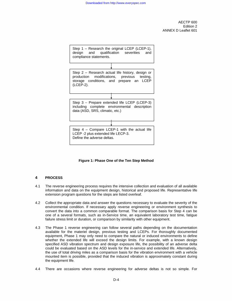
Figure 1: Phase One of the Ten Step Method

4 PROCESS

4.1 The reverse engineering process requires the intensive collection and evaluation of all available information and data on the equipment design, historical and proposed life. Representative life extension program questions for the steps are listed overleaf.

4.2 Collect the appropriate data and answer the questions necessary to evaluate the severity of the environmental condition. If necessary apply reverse engineering or environment synthesis to convert the data into a common comparable format. The comparison basis for Step 4 can be one of a several formats, such as in-Service time, an equivalent laboratory test time, fatigue failure stress limit or duration, or comparison by similarity with other equipment.

4.3 The Phase 1 reverse engineering can follow several paths depending on the documentation available for the materiel design, previous testing and LCEPs. For thoroughly documented equipment, Phase 1 may only need to compare the natural or induced environments to define whether the extended life will exceed the design limits. For example, with a known design specified ASD vibration spectrum and design exposure life, the possibility of an adverse delta could be evaluated based on the ASD levels for the in-service and extended life. Alternatively, the use of total driving miles as a comparison basis for the vibration environment with a vehicle mounted item is possible, provided that the induced vibration is approximately constant during the equipment life.

4.4 There are occasions where reverse engineering for adverse deltas is not so simple. For

Step 1 – Research the original LCEP (LCEP-1), design and qualification severities and compliance statements.

Step 2 – Research actual life history, design or production modifications, previous testing, storage conditions, and prepare an LCEP (LCEP-2).

Step 3 – Prepare extended life LCEP (LCEP-3) including complete environmental description data (ASD, SRS, climatic, etc.)

Step 4 – Compare LCEP-1 with the actual life LCEP -2 plus extended life LECP-3. Define the adverse deltas.


AECTP 600


D-5

example, the lack of a clear comparison basis to quantify adverse deltas may require the evaluator to assume a failure mode (or modes), such as fatigue, and use this failure mode for the Phase 1 evaluation. The assumption of a failure mode in Step 4 of Phase 1 is simply a mechanism to evaluate deltas when other options do not exist. It does not replace the need to undertake the full evaluation of failure modes in Step 5 (Phase 2). It may also be beneficial to perform two evaluations with different comparison bases to provide higher confidence in the adverse delta conclusion.

4.5 Examples of reverse engineering for vibration and high temperature environments are attached to this leaflet. These examples are simplified cases that only evaluate one induced environment, but illustrate the typical problems of establishing a comparison basis and the need for reverse engineering in the Phase 1 process. AECTP 600 Annex C and Leaflets 602 and 604 provide reference sources for Physics of Failure, Time Compression and other modelling techniques.

Typical Information Requirements Applicable for AECTP 600 Phase 1

Step 1

• What was the original equipment qualification requirement?

• What environmental simulation qualification tests were performed on the equipment?

Step 2

• What is the actual in-service environment history of the equipment up to the present date?

• Have any design, hardware, or configuration changes occurred during the service life?

• What are the maintenance and failure rate histories of the equipment?

• What environmental simulation re-qualification or production acceptance tests were performed on the equipment?

Step 3

• Is the extended-life in-service environment defined or a complete LCEP available?

Step 4

• Can the original qualification and historical life information be expressed in the same format as the proposed extended life information? If not, reverse engineering or transformation of the data formats is necessary to a common basis.

• Is sufficient detailed information available to reach a definitive conclusion in Step 4? If not, synthesis of design or actual life environments is necessary to permit evaluation of the information.


AECTP 600


D-6

Reverse Engineering Example 1 - Vibration Environment

Life Extension Requirement – A tracked vehicle electrical relay panel (ERP) was designed and qualified for tracked vehicles 20 years ago with swept sine and sine dwell vibration testing. The ERP is an electro-mechanical hardware component consisting of voltage regulation, switching electronics and circuit breaker functions and mounted in the vehicle crew compartment. The proposed life extension requirement is to field the ERP for an additional 10 years or for 30,000 kilometres on the same or a similar configuration tracked vehicle. The vibration environment for the vehicle is currently quantified as swept narrow band random on random (NBROR) vibration. Is the planned continued utilisation of the ERP hardware acceptable without equipment redesign and re-qualification testing?

AECTP 600 Phase 1 Evaluation – This example addresses only the vibration environment, and omits answers to some Phase 1 questions. The vehicle mission deployment time is a common basis for evaluation of the equipment. The original sine vibration tests will be converted to operational hours for comparison. A complete evaluation would need to evaluate all factors such as the thermal environment, EMI/RFI stability. Following the general reverse engineering questions listed above, current research information and remaining evaluation questions are presented below.

Step 1

What was the original equipment qualification requirement?

• The original requirement defines the equipment specification as a 20 year life on a tracked vehicle. Required reliability is 99.9 % for an average operational time (mission, training, and maintenance) of 1500 hours/year.

What environmental simulation qualification tests were performed on the equipment?

• An operational laboratory logarithmic swept sine vibration qualification test was performed on one ERP from 5 to 500 Hz, at 5 g peak to peak, for a duration of 500 hours in three orthogonal axes.

• An operational laboratory sine dwell qualification test was performed on one ERP for the frequencies of 75, 150, 225 Hz at 5 g peak to peak, for a duration of 30 minutes in three orthogonal axes.

• Equipment field reliability and maintainability tests were performed for one vehicle on paved and off-road conditions for various vehicle speeds during the vehicle development program. No problems were encountered during these initial trials.

• How many miles does the sine sweep represent? (Leaflet 602 time decompression is applied below)

Step 2

What is the actual in-service environment history of the equipment up to the present date?

• On what platform(s) was the ERP used? Two related tracked vehicles.

• What was the total exposure time and mileage? Average annual vehicle operational and deployment time for mission, training and maintenance is 1620 hours/year.

• What was the distribution of the life profile? Which part of the distribution should be used?

• In what geographic location(s) were the vehicles used? World-wide deployment.

• What are the estimated vibration levels associated with the in-service environment(s) for the


AECTP 600


D-7

vehicle? Current available data indicates a typical 5 to 500 Hz random level of less than 2.0 and 0.6 g rms for the vertical and horizontal or transverse axis respectively.

• Was the in-service environment, training, peace-time or war-time use? Both

• Was the ERP used only as intended? Yes

• Are there any special circumstances associated with the types/skills of the users? No

Have any design, hardware, or configuration changes occurred during the service life?

• Check with the program manager, test engineers and manufacturer(s).

• Were any design changes intended to correct vibration related problems? No

• Did design changes invalidate the qualification testing? Unknown

• Was there more than one manufacturer for the ERP in-service conditions? A second source supplier started manufacturing and supplying the unit after 15 years. Qualification tests were not performed for the second supplier ERP.

• Is there product consistency in the fielded units? Original and second source units are fielded.

What are the maintenance and failure rate history of the equipment?

• Use this information to validate the qualification testing.

• Use this data to focus on the critical component parts.

• Does the maintenance history invalidate the historical data?

Logistics and field user information indicate acceptable reliability for the ERP but, occasional intermittent electrical circuit failure problems of unknown origin. Maintenance records for failed units do not indicate specific sub-component reliability problems.

What environmental simulation re-qualification or production acceptance tests were performed on the equipment?

• A cycled operational laboratory logarithmic swept sine vibration operational lot production acceptance test was performed from 5 to 500 Hz, at 5 g peak to peak, for a duration of 24 hours in three orthogonal axes.

• A cycled operational laboratory sine dwell operational lot production acceptance test was performed for the frequencies of 75, 150, 225 Hz at 5 g peak to peak, for a duration of 30 minutes in three orthogonal axes.

Step 3

Is the extended-life in-service environment defined or a complete LCEP available?

• Vehicle maintenance and future upgrades are not expected change the vibration severity of the vehicle.


AECTP 600


D-8

• The estimated vehicle operational time and mileage per year in LCEP-3 is the same as current in-service life LCEP-2, 1620 hours/year operation expected.

Step 4

Can the original qualification and historical life information be expressed in the same format as the proposed extended life information?

• Convert data from the qualification, actual life and extended life into an exposure time basis

• An alternative approach would be to correlate the sine vibration qualification testing with the current NBROR environment.

Is sufficient detailed information available to reach a definitive conclusion in Step 4?

• If the sum of the historical and life extension damage potential indicates a risk of failure, then there is an adverse delta.

• Consider all mitigating data or circumstances.

Exposure Time Evaluation

With the information known and the assumptions below the exposure duration for the ERP in Steps 1-3 are summarised in the table below.

Assumptions:

1. The three axis vibration tests replicate field multi-axis vibration exposure. The calculated qualification test duration is based on one axis of the testing, 500 hours.

2. Material property factors for the ERP conform to typical electrical-mechanical hardware.

3. Material fatigue is the primary failure mode for the equipment.

Equivalent field exposure time for the sine sweep and dwell qualification tests is calculated from the application of Miner’s Rule with material factors of the stress-cycle exponent b = 9, damping exponent n = 2.4, and an acceleration exaggeration factor of 2.0.

TABLE 1 – SUMMARY OF EXPOSURE TIME

Step Number

Test or Exposure Equivalent Time, hours

Time Summation, hours

1 Design Requirement, 20 yr, 1500 hr/yr n/a 30,000 Qualification tests : Swept Sine, 5 g peak, 500 hrs. 45,225 Sine Dwell, 75, 150 225 Hz, 30 min./dwell 136 45,391

2 Production Tests, Sine Sweep & Dwell 2308 Field Deployment, 20 yrs, 1620 hr/yr 32,400 34,708

3 In-service life, 20 yrs 34,708 Extended life, 10 yrs, 1620 hr/yr 16,200 50,908


AECTP 600


D-9

Conclusion

Exposure times in Table 1 indicate the sine sweep and dwell qualification tests demonstrate an adequate exposure time (45,391 hours) exceeding the 30,000 hour design value for the ERP tests. Actual in-service exposure also is greater than 30,000 hours, however Step 2 logistic reports also indicate intermittent some field failures in current units. An additional 10-year field deployment of the existing ERP would result in an exposure time that exceeds the current laboratory equivalent vibration simulation testing time; the delta is 5571 hours or approximately 3 years.

Based on the preliminary information, the vehicle operation vibration exposure is considered an adverse delta for a 10 year ERP extended life requirement. Several factors also influence the decision. The qualification tests were performed only on one ERP unit rather than a larger sample size to provide a greater data confidence. The qualification tests were not performed under controlled climatic conditions to demonstrate the worldwide deployment reliability of the ERP.

A direct comparison of the equivalence between sine and random vibration exposure is another option, but subject to debate depending on the assumptions made and choice of equivalence calculations. Accurate correlation between the previous sine qualification test technology and current random NBROR vibration technology is difficult to permit demonstration that the original tests meet the actual environment.


AECTP 600


D-10

Reverse Engineering Example 2 - High Temperature Environment

Life Extension Requirement – A vehicle voltage regulator, installed in the engine compartment, was designed and qualified for two tracked vehicles (T1 and T2) 20 years ago. The proposed life extension requirement is to field the voltage regulator an additional 5 years (25,000 km) on tracked vehicle (T2) that will be required to operate in a high ambient temperature (+50 ºC) geographical region. Is the planned utilisation of the voltage regulator on vehicle T2 acceptable without equipment redesign and re-qualification testing?

AECTP 600 Phase 1 Evaluation – For this case the qualification tests were based on vehicle temperatures and do not state an ambient temperature condition. The original design and qualification information will be evaluated to reverse engineer a high temperature ambient design condition.

Following the general list of reverse engineering questions, current research information and remaining evaluation questions are presented below.

This example deals only with reverse engineering techniques and most of the details have been removed. For this device the operational environment is assumed to be more severe than the storage environment. Other issues related to performing Steps 2 and 3 are addressed in Leaflet 605.

Many of the temperatures are stated in degrees Fahrenheit rather than degrees Centigrade to provide a more realistic example from legacy requirements and test results.

Step 1

What was the original equipment qualification requirement?

• The original requirement defines the equipment specification as a 20 year life on two tracked vehicles (T1 and T 2) with an operational temperature range of –60 to +250 ºF, and relative humidity of 5 to 95 % at 140 to 40 ºF. The storage temperature requirement is –60 to +130 ºF.

What environmental simulation qualification tests were performed on the equipment?

• A 3000 hour + 280 ºF steady state operational qualification test was performed

• A 240 hour (10 cycles) aggravated temperature/humidity test was performed. The climatic cycle was +60 ºF to + 140 ºF with 95 % RH.

• 48 hour non-operational steady state tests were performed at temperatures of –60 ºF and +130 ºF.

Step 2

What is the actual in-service environment history of the equipment up to the present date?

• On what platform(s) was the regulator used?

• What was the total exposure time and temperature, operational and non-operational?

• What was the distribution of the life profile? Which part of the distribution should be used?

• In what geographic location(s) were the vehicles used?

• What are the ambient temperatures of the associated with the in-service environments?


AECTP 600


D-11

• What was the in-service environment, training, peace-time or war-time use?

• Was the regulator used only as intended?

• Are there any special circumstances associated with the types/skills of the users

Have any design, hardware, or configuration changes occurred during the service life?

• Check with the program manager, test engineers, or manufacturer(s).

• Were any design changes intended to correct thermal related problems?

• Did design changes invalidate the qualification testing?

• Was there more than one manufacturer for the regulator?

• Is there product consistency in the fielded units?

What are the maintenance and failure rate history of the equipment?

• Use this information to validate the qualification testing.

• Use this data to focus on the critical component parts.

• Does maintenance history invalidate previous history data?

What environmental simulation re-qualification or production acceptance tests were performed on the equipment?

• A 24 hour + 280 ºF steady state operational lot production acceptance test was performed

Although the answers to the questions above are applicable to the overall Ten Step Method, in this example the answers were simplified because the in-service use time and severities were less than the design requirement.

Step 3

Is the extended-life in-service environment defined; or a complete LCEP available?

• A thermal measurement program for T2 has been performed and data is available for review.

• A specification has been developed for the new operational temperature data.

• An estimation of the operational time use per year and associated ambient temperature is available.

A temperature LCEP-3 was developed from measured data for use in this example. The LCEP-3 presented the data as extremes and an average diurnal cycle

Step 4

Can the original qualification and historical life information be expressed in the same format as the proposed extended life information?

• Convert data from the qualification, history and new environments into terms of equivalent degradation, an Arrhenius Equation for example. How many in-service hours do the qualification tests equal? In some cases the environmental conditions provided will not make


AECTP 600


D-12

sense. In these cases engineering judgement must be used, and it might not be possible to exploit all the test results.

• In this example an alternate format was used which takes advantage of documented available analytical procedures.

• Additional method would be to use the cyclic stresses, however original qualification did not provide a detailed cyclical criteria, therefore no basis for comparison exists.

Is sufficient detailed information available to reach a definitive conclusion in Step 4?

• If the sum of the historical and life extension severities indicates a risk of failure, then there is an adverse delta.

• Consider all mitigating data or circumstances.

In this reverse engineering example the task in Step 4 is to convert the data from Steps 1 through 3 into a common format. Since the LCEP-3 presented the data in terms of extremes and a diurnal cycle the next logical step is to convert data from Steps 1 and 2 into common terms. In order to address potential failure modes there is a need to address both chemical aging and thermal stresses. Magnitude of the temperature extremes and the number of temperature reversals are critical in the evaluation of thermal mechanical stresses, while the total time at high temperature is critical to the evaluation of chemical deterioration. (More information can be found in Leaflets 602 and 604).

The original storage test (280 ºF for 3000 hours) and the successful 20 year high temperature exposure history indicate that any adverse deltas would be derived from cyclic thermal stresses rather than steady-state high temperature exposure. To evaluate those stresses, it is necessary for all data to be presented in some common applicable format. For this example, fatigue damage due to thermally induced mechanical stress was taken as the common format, and all test and life history cyclic temperature data is converted into a relative measure of fatigue damage as shown in the example.

Thermal-Mechanical Stress Evaluation:

In Step 1 the data shows that during qualification testing a total of 10 stress reversals with an 80 ºF delta each were performed. Additionally one stress reversal with a 130 ºF delta and one stress reversal with a 60 ºF delta were performed.

Step 2 logistics reports have shown that the regulator demonstrated 99% reliability during 200 days of operation in a desert region (+70 ºF to +250 ºF, 200 cycles). In addition 90% reliability with a 20 year service life in an average temperate cycle (+60 ºF to +220 º F, 1000 cycles) was demonstrated for a sample of 1,000 units.

In Step 3 the extreme temperatures measured were –20 ºF to +250 ºF, the operational low temperature cycle ranges from –20 ºF to +120 ºF for 100 cycles and a high temperature cycle ranges from +70 ºF to 250 ºF for 400 cycles.

This information is summarised in Table 1 below. Note that the letter-number designations under the Storage and Transport column refer to climatic region designations as per STANAG 2895.


AECTP 600


D-13

TABLE 1 – STORAGE AND TRANSPORT AND DEPLOYMENT CONDITIONS

Step Number

Storage & Transport Deployment

Step 1 -60 ºF for 48 hrs 130 ºF for 48 hrs

280 ºF for 3000 hrs 60 ºF to 140 ºF 95% RH, 240 hrs

Step 2 A2, A3, B2, C0 C1 20 years 90% RH A2, A3, B2, C0, C1 10 yrs 99% RH B3 200 days

280 ºF for 24 hr LAT 70 ºF to 250 ºF 200 cycles 60 ºF to 220 ºF 1000 cycles

Step 3 A2, A3, B2, C0, C1 5 year, 90% RH B3 200 days 90%

-20 ºF to 250 ºF extremes -20 ºF to 120 ºF 100 cycles 70 ºF to 250 ºF 400 cycles

There are many different approaches to assess this situation however a rudimentary approach could be to use the basic Miner-Palmgren cumulative damage hypothesis (see Leaflet 602 for details) to determine if the thermal stress cycling revealed in Step 2 is sufficient to cover the new LCEP.

Assumptions used in the Miner-Palmgren analysis:

The number of cycles to failure for any given stress range can be estimated from:

Ni = c∆Si-b

The damage for any stress range can be calculated as the number of actual cycles at that stress range divided by the allowable number (Ni) at that range

Di = ni/NI

The total damage for any condition (eg: Step 3) can be computed as the linear sum of the damage for each stress range within that condition

D = ΣDi

The stress range is linearly proportional to the temperature range (Reference 20, Annex C, Section 1) ∆S ~ k∆T, thus, Ni = ck∆Ti

-b

The rate of change in temperature and the temperature range (delta) is approximately the same between Steps 1, 2 and 3

A material constant of b = -5 is used. This provides a conservative estimate of the comparison, and is used because of the small number of cycles (<1000 cycles)

A relative measure of damage between two conditions can be described by:

D1/D2 = (n1/N1)/(n2/N2) = n1N2/n2N1 = n1/n2*N2/N1 = n1/n2 * (∆T2/∆T1)-b

The equivalent damage can be compared for each cyclic condition versus some reference condition (eg: the 400 cycle section of Step 3), and the damage for each step can be summed and compared to the sum of the damage for Step 3.


AECTP 600


D-14

TABLE 2 – THERMAL CYCLE DAMAGE

Step Number

Temperature Cycling Damage relative to 400 Cycles of Step 3

Step 1 Ambient to -60 ºF for 48 hrs (1 cycle) Ambient to +130 ºF for 48 hrs (1 cycle) 60 ºF to 140 ºF, 10 cycles

0.00049 0.00001 0.00043

Step 2 70 ºF to 250 ºF 200 cycles 60 ºF to 220 ºF 1000 cycles

0.5 1.387

Step 3 -20 ºF to 120 ºF 100 cycles 70 ºF to 250 ºF 400 cycles

0.071 1.000

TABLE 3 – THERMAL DAMAGE SUMMATION

Step Number

Total Relative Damage Damage relative to Step 3

Step 1 .00093 0.00087 Step 2 1.887 1.762 Step 3 1.071 1.000

From the above tables, it is demonstrated that the testing performed for Step 1 was insufficient to address the requirements of Step 3, but the successful history demonstrated in Step 2 indicates that the regulator has a significantly longer life (re temperature cycling) than that required for Step 3. New regulators or existing regulators with an in-service life less than the extreme examples shown in Step 2 will meet the Life Extension requirements shown in Step 3. To assess the thermal /chemical degradation a similar process could be performed using the Arrhenius equations.

Conclusion

In this example it has been concluded from the reverse engineering process that the thermal environment does not create an adverse delta. If no other adverse deltas were determined an Exit Criteria 1 could be applied.


AECTP 600


D-15

LEAFLET 602 - TIME COMPRESSION

1 SCOPE

1.1 This leaflet addresses commonly used time compression techniques, and provides guidance and limitations on how to perform reverse time compression for the purpose of estimating original measured in-service levels (see Leaflet 601) or for providing a common time based comparison of different environments. It provides a link to the available bibliography information and to STANAG 4370 AECTP 200 Leaflets 2310 and 2410. Examples of environmental conditions where time compression is appropriate and not appropriate are provided.

2 DEFINITION AND BACKGROUND

2.1 Time compression is the process of increasing the rate of degradation of materiel in a quantitative manner. The goal is to shorten the test time by increasing the severity of the environment using a physics-based method that retains the correct failure mechanisms without inducing others. When applied properly, time compression is a reversible process (ie: the rate of degradation can be increased or decreased).

2.2 As stated in AECTP 600 Paragraph 5.4.3, time compression or decompression techniques are needed to aid comparison of levels. Also as stated in AECTP 600 Paragraph 5.8.2, the techniques are required for tailoring test severities to make a cost effective test. This technique is an integral part of the reverse engineering process.

3 LIMITATIONS

3.1 The following limitations and cautions should be noted when considering the use of time compression techniques:

• some test severities were not originally based upon time compression and, therefore, are not reversible

• documentation of the original time compression may not be available and consequently the assumptions and techniques utilised may not be understood

• the relationship of the physics of failure mechanisms to time compression is not always sufficiently understood for failure modes to be predicted accurately

• the traceability of time compression techniques used for some test programmes may be unknown

• the complexity of the materiel is such that separating failure modes for time compression is difficult

• care must be taken to ensure that increasing amplitudes to shorten test time does not change failure modes

4 TIME COMPRESSION – MECHANICAL ENVIRONMENTS

4.1 General

4.1.1 Time compression can be achieved in a dynamic mechanical environment using frequency domain and time domain techniques. Both are based on equivalent fatigue between the in-service environment and the test environment and are based on forms of the Miner-Palmgren cumulative damage hypothesis. In the frequency domain, time compression is usually accomplished through the application of an 'exaggeration factor', while the technique in the time domain is known as 'fatigue editing'. The frequency domain techniques preserve the spectral


AECTP 600


D-16

content (and thus the system transfer function, if conducted properly), but makes the assumption that material stress is linearly proportional to acceleration across the spectrum. It is applicable to situations where the failure may occur at some location away from the measurement location (eg: a circuit card in a radio where the measurement is performed at the input to the radio structure). Fatigue editing does not preserve the frequency content of the data, and is generally applicable for testing the same component for which a strain measurement was made (eg: vehicle suspension control arm when in-service and in a laboratory test).

4.2 Frequency Domain Technique

4.2.1 It is preferable for materiel to be tested in real-time so that the effects of in-service conditions are simulated most effectively. However, in many instances real-time testing cannot be justified on cost grounds, and therefore it is customary to use an acceptable algorithm to reduce test duration by increasing test amplitude. Provided that fatigue is a significant potential failure criterion for the materiel under test, then this practice is acceptable within strict limits, notably that test amplitudes are not over exaggerated (or accelerated) simply to achieve short test durations. Such excessive amplitudes may lead to wholly unrepresentative failures and cause suppliers to design materiel to withstand arbitrary tests rather than the in-service conditions. Therefore any reduction in test duration should be restricted to increasing the test amplitude only to the limit severities derived for the in-service conditions. Within this constraint considerable scope usually exists for reducing test duration.

4.2.2 The most commonly used method for calculating a reduction in test duration is the Miner-Palmgren hypothesis, ie:

Equation (1)

where t1 = equivalent test time t2 = in-service time for specified condition S1 = severity (rms) at test condition S2 = severity (rms) at in-service condition n = slope of the S/N curve for the appropriate material; a value of 5

is commonly used (See AECTP 200, Leaflet 2410, Annex B, Paragraph 2.2).

4.2.3 Since most vibration environments are expressed in terms of the power spectral density function, equation 1 can also be used as:

n/2

W(f)W(f)

tt

1

2

2

1⎥⎦

⎤⎢⎣

⎡=

Equation (2)

where t1 = equivalent test time t2 = in-service time for specified condition W(f)1 = PSD at test condition W(f)2 = PSD at in-service condition

n = slope of the S/N curve for the appropriate material; a value of 5 is commonly used (See AECTP 200, Leaflet 2410, Annex B, Paragraph 2.2).

4.2.4 In many instances these equations appear to offer a satisfactory solution. However, caution should always be exercised in the application of the equations. Some methods of characterising


AECTP 600


D-17

vibration severities, notably PSDs, do not necessarily reproduce under laboratory testing the same strain responses as those experienced under in-service conditions.

4.3 Time Domain Technique

4.3.1 The time compression technique performed on time domain data is also fatigue equivalence based, but uses a process of fatigue editing rather than amplitude exaggeration. The technique is applied to data measured as strain rather than acceleration. A cycle counting technique such as 'rainflow' counting is performed on the time series data, and a fatigue damage value is computed from the results of the rainflow histogram. Thus, it is possible to assign a fatigue damage value to different test conditions or to different sections of a long data record. Time compression is achieved by eliminating all test conditions or sections of a data record that do not contribute to the overall fatigue damage. The edited sections of the overall data set are then joined to make a time-reduced, but equivalent fatigue damage version of the original record.

5 TIME DECOMPRESSION – MECHANICAL ENVIRONMENTS

5.1 It is important to realise that time decompression is only valid if the failure mechanisms are unaffected by the decompression and that the rate of change in degradation is predictable between the compressed and uncompressed values. This will only be true over a limited range of decompression where non-linearities are not significant. Non-linear (dynamically) joints and rattling components for example are not good candidates for decompression unless the maximum factored measured data are well understood.

5.2 Care should be taken when attempting to decompress a test schedule. It is unwise to decompress to the point where the decompressed result are less severe, at some part of the frequency spectrum, than the maximum factored measured data.

6 TIME COMPRESSION – CLIMATIC ENVIRONMENTS

6.1 General

6.1.1 With regard to temperature and humidity in a natural environment the duration of exposure for most materials is such that real time testing is not an option. Therefore testing is only practical for these environments using some form of time compression. Time compression of climatic environments can be achieved where there is a single dominant chemical degradation mechanism of a component material that is temperature, or temperature and humidity, dependant. There are many forms of the time compression model and their applicability is dependant upon the dominance of certain aspects of the chemical reactions taking place.

6.1.2 All models are essentially based upon an exponential relationship with the activation energy (Ea - the minimum amount of energy required to enable the reaction) in the exponent. If the activation energy of the dominant mechanism within the material is not known then time compression cannot be achieved. Stabiliser depletion (Ea 100+ kJ/mole), oxidisation (Ea 76-96 kJ/mole), plasticiser migration (Ea 75-85 kJ/mole) and diffusion of moisture (Ea 70 kJ/mole) are known degradation mechanisms that can be adequately simulated through this form of time compression. Compression can be calculated because the relationship between temperature and time is log-linear. This will only be true for a very narrow temperature range. Compression models, which go outside this temperature range, are inappropriate either because of inherent non-linearity in the material such as step changes (eg: glass transition, melting) or because the considered degradation mechanism is no longer dominant at those temperatures.

6.2 Arrhenius-Berthelot-Eyring

6.2.1 A commonly used time compression model is the model initially developed by Berthelot from the Arrhenius equation. This is shown in Equation 3, in its most useful format and includes a Humidity factor, as considered by Eyring:


AECTP 600


D-18

[ ] [ ] ( )HfeettK ××== T2R

EaT1REa-

21

Equation (3)

Where K = the ratio of test time to natural time t1 = the compressed time t2 = the natural time Ea = activation energy R = the gas constant (0.0083143 if Ea is given in kJ/mole) T1 = mean (rationalised) temperature during test/compression T2 = mean (rationalised) temperature in the natural environment f(H) = function or factor for humidity, default is 1. (See Ref. 8 of Annex C)

6.2.2 The expression f(H) is a usually unknown modifying function or factor of humidity for the material. It should only be included if it is known and has been proven by experiment.

6.2.3 In many applications this model provides a sufficiently short duration for a test without exceeding the effective temperature range for the chemical processes under investigation. However, care must be taken in applying this model and it should not be applied without good understanding of all the primary chemical, and biological, processes of the constituent materials.

6.2.4 This and most other empirical time compression models should not be used when T1 or T2 are less than 10 ºC or greater than 80 ºC, regardless of material, as the results will be at best misleading and at worst dangerous if used. Some methods of use require a reference temperature. The reference temperature must be either higher or lower than both T1 and T2 and should remain within the temperature range indicated by the degradation process under examination.

6.3 Rationalisation

6.3.1 In very simplistic terms, all of the commonly used compression models equate the overall energy imparted to the material in real environments to the overall energy imparted in a test. Temperature and time can be envisaged as the two dimensions of a rectangle with energy being the area of the rectangle. The models compare the rectangles, and if they have the same area then the overall degradation of the material is calculated to be the same. Because this is the case, where variation in temperature occurs over the time-period under consideration it is rationalised to give a single temperature for use in the models.

6.3.2 The data needs to be complete, and presented in a format with sufficiently small time steps to provide an adequate description of the continuous environment it was taken from. If this is the case, the data can be rationalised by applying the Arrhenius equation to each discrete time step and averaging this over all the results before converting back to a rationalised temperature. However, the data is not always adequate for this method and therefore maximum, mean, or mean of maximum temperatures often need to be used in the model as a fall back measure. The value to use will depend upon the application, the material, and the confidence in the data available. (See AECTP 200 Leaflet 2310 for a full description of rationalisation of temperature and humidity data.)

6.4 Diurnal Cycling, Fixed Temperature and Aggravated Ageing

6.4.1 In the natural environment, air temperatures follow a distinct daily, or diurnal, cycle. Generally, it is colder during the hours of darkness with the temperature rising steadily to a peak about mid-afternoon before dropping off again, lagging behind the movement of the sun. The most commonly used climatic time compression models do not account for diurnal cycling. However, application of the mechanical time domain technique described above can be used in


AECTP 600


D-19

association with a similar thermal model, if the application requires that level of detail. Regardless of the models, it is good practice to include diurnal cycling within any test program. The changes in temperature can expose real weaknesses in the material associated with differential expansion and gas diffusion that would not be seen with a single, rationalised, temperature. However these failure mechanisms are sensitive to the rate of change of temperature as well as the overall energy imparted, because of this diurnal cycles employed should not be different from those seen in the natural environment. The '1% maximum' cycle for the hottest climatic region in which the material will find itself is often found to be the most effective profile to employ for time compression.

6.4.2 In most cases fixed temperature ageing should only be used to represent storage in long term or temperature controlled depots. It is not appropriate for simulating storage or use in the full natural environment as it does not exercise the material thermo-mechanically. Diurnal cycling should be the preferred method for time compressed testing, unless there is a fully understood mechanism, which renders a material particularly sensitive to temperature cycling.

6.4.3 It is not appropriate to use aggravated temperature cycling in tests where time compression/decompression is necessary. Aggravated cycles where either the rate of change or the maximum (minimum) temperature (or humidity) exceeds the natural maximum level cannot be compressed/decompressed as there is no direct comparison that can be drawn between the compressed and decompressed profiles. Aggravated cycles are only really appropriate in pre-cursor testing or experimentation where the material properties are under close examination for measurement against a standard, prior to introduction to a new system.

7 TIME DECOMPRESSION – CLIMATIC ENVIRONMENTS

7.1 It is important to realise that, as in time compression, time decompression is only valid within the appropriate temperature range and if the dominant degradation mechanism is known to remain the same in both the compressed and decompressed environments.

7.2 Care should always be taken when attempting to decompress a test profile. After all if a fertilised chicken egg were heated at 95 ºC for 10 minutes the result would be a hard-boiled egg. If the same egg were heated at 37 ºC for three weeks the result would be yellow and running around the ground going 'Cheep'!


AECTP 600


D-20

INTENTIONALLY BLANK


AECTP 600


D-21

LEAFLET 603 - INCREMENTAL ACQUISITION

1 SCOPE

1.1 Incremental acquisition enables planned upgrades to be incorporated into materiel procurement programmes where improvements in technology are expected during the service life of the system and significant benefits in terms of safety and/or performance would be achieved by incorporating such technology. This activity must be addressed at the earliest possible stage of the procurement programme, and should not to be confused with mid-life upgrades which are applicable to equipment that is already in service.

1.2 This leaflet provides guidance on the strategy that should be adopted during the incremental acquisition of materiel and on how the Ten Step Method can be used to aid the management of this process .

2 APPLICABILITY

2.1 This leaflet is applicable to all materiel procurement programmes in which significant developments in the design of the system (during its service life) are planned from the outset.

3 BACKGROUND

3.1 Incremental acquisition can have significant benefits to a procurement programme in that it is intended to reduce the time taken to introduce new key technologies into service. Although this does not itself represent an extended life requirement, it is considered that the tools of the Ten Step Method lend themselves to the management of this process.

3.2 Any new procurement programme involving incremental acquisition should adopt the principles of the Ten Step Method from the outset. Thus the materiel should be developed and qualified to a recognisable form of environmental engineering control and management process such as those presented in STANAGs 4370 and 4570 and their associated AECTPs. Even if this is not the case, it should be possible to apply this process to any technically credible methodology provided that the relevant information can be re-configured to align with the Ten Step Method in AECTP 600.

3.3 Provided no role or deployment changes are invoked, then the 'deltas' in Step 4 will essentially be the original Life Cycle Environmental Profile (LCEP), but the life requirement may be reduced. If role or deployment changes are invoked then there will be changes to the LCEP and the guidance given in AECTP 607 should be followed.

3.4 Incremental acquisition provides for equipment capability to be upgraded in a planned way, from the initial delivery of a specified minimum acceptable performance to the eventual achievement of target performance, thereby.

• Reducing the risks relative to those associated with traditional procurement methods, in which large improvements in capability are introduced in a single major technological step, and reducing the risk of delivering obsolescent equipment and cost over-runs.

• Allowing systems to be developed and put into service that will incorporate evolving technology as it becomes available, thus speeding up the introduction of new technology into service.

• In very fast moving technologies (such as software intensive projects) allowing systems to be developed with an open architecture to take maximum advantage of new opportunities.


AECTP 600


D-22

3.5 Incremental acquisition, planned from the outset, is quite distinct from the application of mid-life upgrades to existing equipment. These are dealt with through the normal operation of a new acquisition cycle and arise when it is decided, after examining all available options, that a requirement for additional capability is best satisfied by the upgrading of existing in service equipment. These activities are planned, approved and conducted as projects in their own right.

3.6 An example using a generic Medium Range Air-to-Air Missile (MRAAM) system is appended to this leaflet to demonstrate the application of this outline approach.

4 IMPLICATIONS AND CONSTRAINTS

4.1 The following issues need to be addressed when considering the procurement of materiel using incremental acquisition:

• the materiel must be designed to facilitate the incorporation of the upgrades

• all potential interactions between the upgrade and the system must be considered from the outset, eg: mass, centre of gravity, electrical power requirements, software, interfaces, etc

• evidence will be required to demonstrate to what extent the upgrade meets the requirements of the system in terms of performance, safety, environmental conditions, life, etc

• life requirements for individual sub-systems may be less than the overall life of the system

• stock control and asset tracking procedures must be implemented to ensure that information is available on the build standard and service history of all assets and components

• staggering the purchase of missiles over a number of years may aid the management of the upgrade programme


AECTP 600


D-23

Example - MRAAM Missile System

Requirement

The requirement is to introduce the missile with an agreed baseline capability and an initial system life of 10 years (to be extended to 15 years).

Planned upgrades are: an enhanced seeker after 3 years in service, an enhanced safety and arming unit (SAU) after 6 years in service, and an enhanced rocket motor after 8 years in service.

An outline of the planned schedule is given in Figure 1.

Concept and Design

The user and system requirements are produced and the decision is made to procure the MRAAM system using incremental acquisition.

Industry involvement is sought and a single contractor selected.

Baseline Capability

The ability of the missile to meet the safety, performance, environmental and life requirements is assessed using the principles of the Ten Step Method.

All elements of the system are certified/qualified/approved as safe and suitable for service. (This may be achieved by allocating an initial life (eg: 5 years) for each element, with phased increases in life based on further testing, surveillance and assessments).

First Acquisition Increment (after 3 years in service)

An enhanced seeker unit is developed in accordance with the agreed time scales. Following demonstration of the ability of the unit to meet the performance and integration requirements an environmental and life assessment programme is conducted. This is achieved using of the Ten Step Method, modified as follows:

Step 1 The original LCEP was determined during concept and design phase

Step 2 N/A

Step 3 Prepare LCEP for remaining life of the missile based on the original LCEP

Step 4 The ‘deltas’ for the seeker are effectively the output from Step 3

Step 5 Identify the possible failure modes for the seeker unit and determine which produce potentially critical cases

Steps 6 to 9 are as for the standard Ten Step Method

Step 10 Evaluate the results of the tasks and compile a life statement for the seeker unit assessing to what extent the requirement is met

In this case only limited additional testing is required and the life statement is based mainly on analyses and assessments.


AECTP 600


D-24

Second Acquisition Increment (after 6 years in service)

An enhanced SAU is developed in accordance with the agreed time scales, but integration problems result in minor mechanical design modifications. Following approval of these modifications an environmental and life assessment programme is conducted by following the modified Ten Step Method:


Step 2 N/A


Step 4 The “deltas” for the SAU are effectively the output from Step 3

Step 5 Identify the possible failure modes for the SAU and determine which produce potentially critical cases


Step 10 Evaluate the results of the tasks and compile a life statement for the SAU assessing to what extent the requirement is met

As the SAU contains energetic components and performs a primary safety function in the missile design, more stringent treatment including significant testing is required. This includes mandatory safety tests, performance and reliability tests, testing to simulate the LCEP and includes accelerated ageing to assess the life of the energetic components.

Third Acquisition Increment (after 8 years in service)

An enhanced rocket motor is developed, but delays in the programme mean that a life extension programme is required for the original motor to the end of Year 10. This life extension element is carried out in accordance with the standard Ten Step Method.

Once the design issues of the enhanced rocket motor are resolved, additional treatment is carried out in accordance with outputs of the modified Ten Step Method:


Step 2 N/A


Step 4 The ‘deltas’ for the rocket motor are effectively the output from Step 3

Step 5 Identify the possible failure modes for the rocket motor and determine which produce potentially critical cases


Step 10 Evaluate the results of the tasks and compile a life statement for the rocket motor assessing to what extent the requirement is met

Due to the quantity of energetic material in the rocket motor and the potential consequences of any accident, stringent treatment including significant testing is required. The life assessment statement covers the rocket motor for the full remaining life of the missile (ie: out to 15 years service).


AECTP 600


D-25

Life Extension (after 10 years in service)

At Year 10 all upgrades have been completed and the stockpile consists of a single design standard. To accommodate the energetic components the life extension requirement to 15 years is met directly through the application of the standard Ten Step Method in two phases (see Figure 1). However, note that in this case the enhanced rocket motor does not require any life extension.


AECTP 600


D-26

INTENTIONALLY BLANK


AECTP 600


D-27

Figure 1: Planned Incremental Acquisition Schedule for MRAAM

Missile System - Years in Service Incremental Acquisition Phase

0 1 2 3 4 5 6 7 8 9 10 11 12 13 14 15

Establish Baseline Capability •

Introduction into Service •

1st Acquisition Increment - Development • •

1st Acquisition Increment - Demonstration • •

1st Acquisition Increment - Introduction into Service

•

2nd Acquisition Increment - Development • •

2nd Acquisition Increment - Demonstration

• •

2nd Acquisition Increment - Introduction into Service

•

3rd Acquisition Increment - Development • •

3rd Acquisition Increment - Demonstration • •

3rd Acquisition Increment - Introduction into Service

•

Life Extension - Phase 1 •

Life Extension - Phase 2 •

Remove from Service •

Note: Schedule assumes a single batch of missiles is purchased in Year 0


AECTP 600


D-28

INTENTIONALLY BLANK


AECTP 600


D-29

LEAFLET 604 - PHYSICS OF FAILURE

1 SCOPE

1.1 The purpose of Leaflet 604 is to provide guidance on the use of Physics of Failure (PoF) techniques to determine if the environmental conditions associated with adverse deltas will precipitate critical failures based upon the life extension requirements.

2 DEFINITION

2.1 Physics of Failure is a mathematical representation of the relationship between environmental stresses and failure mechanisms. This approach models the root causes of failure such as fatigue, fracture, wear and corrosion.

3 BACKGROUND

3.1 Computer-Aided Design (CAD) tools have been developed to address various material failure mechanisms and locations. PoF provides the ability to determine the amount of ‘life' already used by a system in-service by relating time spent in a particular environment to the amount of damage accumulated.

3.2 To apply a life extension strategy effectively, the engineer will need to know not only the relevant failure mechanism to be predicted by PoF based models, but also the actual in-service load conditions the system is experiencing. It is, therefore, necessary to develop a PoF process methodology that will ensure that the right operational and environmental data are being or have been collected for PoF fatigue and wear models. This is important because:

• failures are time and amplitude dependent so it is not possible to make quick assessments

• the PoF process allocates environmental stress levels down to a component that has been determined to be critical

• the PoF process allows you to focus on critical deployed (mission use) environmental conditions

• the PoF process links the synergistic effects (such as temperature, humidity and vibration)

• the PoF process allows evaluation of alternative design ideas or environmental mitigation techniques

• the PoF process provides a quantitative answer - not just pass or fail

4 LIMITATIONS

4.1 The limitations of this approach are:

models are deterministic rather than stochastic

models need to be validated through testing

models cannot replicate workmanship issues


AECTP 600


D-30

5 RELATIONSHIP TO AECTP 600

5.1 In Paragraph 5.5.6 of AECTP 600, the application of Physics of Failure processes is required to quantify the relationship between the environmental conditions and the potentially critical failure modes.

6 EXAMPLE OF A PHYSICS OF FAILURE PROCESS

6.1 Physics of Failure is a process that addresses root cause mechanisms and driving forces responsible for equipment failures. Mechanisms can include (but are not limited to) loss of electrical contact or structural degradation due to corrosion, stresses in materials due to dynamic or thermal environments, loss of material due to abrasion or insufficient lubrication and a thermally induced change of material state. The following example of the PoF process applied to a life extension strategy addresses only metal fatigue failure due to exposure to a harsh dynamic environment.


AECTP 600


D-31

Example of a Physics of Failure Process

General

The purpose of this example is to demonstrate the development of a process to calculate the life consumed (ie: damage accumulated) on a critical component of a military trailer. The process is based on modelling the vibration experienced by the trailer starting with a model of the applicable terrain. Specific steps for this process are developed and include a PoF analysis to calculate damage of the trailer as follows:

• development of rigid and flexible-bodied Dynamic Analysis and Design System (DYNAMIC) models of the trailer;

• development of Finite Element Model (FEM) of the trailer;

• various physical measurements of the trailer for model input and verification;

• dynamic measurement and analysis of the trailer to determine acceleration and stress history for the terrain classes selected; and

• life prediction on trailer drawbar (weakest part of trailer) for each of the terrain classes.

The selection of the critical components is a combination of what components are the least reliable and which components are functionally critical to the mission. A combination of general engineering analysis and past field and test data can be used for the selection process. If no past data are available, an engineering analysis can be performed using the known environmental stresses (ie: vehicle vibration, vehicle shock, water, and ground conditions). A simplified finite element analysis can be performed to locate areas of the trailer with high stress.

Modelling process and models

This modelling and simulation effort involves several engineering disciplines, including:

• Computer-Aided Design (CAD) solid modelling;

• Finite element analysis for deformation and stress;

• Multi-body dynamic analysis for dynamic load history simulation;

• Fatigue life simulation for durability analysis; and

• Experimental testing for model validation.

The modelling approach begins by using terrain data gathered by the test centre for use in the dynamic models. Dynamic modelling is used for a rigid-body analysis and a flexible-body analysis using finite element analysis. The flexible-body dynamic model is used to determine the dynamic accelerations at all points on the trailer during a simulated run of the trailer over a given terrain. Finally, the university developed software tool is used to integrate results from dynamic modelling and finite element modelling to determine the stress history, strain history, and fatigue life. The following sections outline the process of how these modelling approaches are applied to the trailer.

Computer Aided Design Model

The process of computationally determining the fatigue life of a mechanical system starts by developing a three-dimensional, parameterized CAD model. Mass and material properties are assigned to each part of the CAD model, and comparison is made to the physical model. This comparison includes the total mass, centre-of-gravity location, and total inertia. It is very


AECTP 600


D-32

important that the CAD model approximates the physical vehicle as closely as possible, since both the finite element and multi-body dynamics computational models will be derived from it. The CAD model also forms the basis for consistency for these other models.

Figure 1: Solid Model of Trailer

Finite Element Model (FEM)

In this PoF approach, the finite element model is used for several purposes. The first purpose is to evaluate the vibration modes, which are used to create the flexible multi-body dynamics model. These simulated modes are compared to an experimental modal analysis survey of the physical trailer to validate the analysis. The second purpose of the finite element model is to evaluate deformations of the trailer, which are used as static correction modes in the flexible multi-body model. The third purpose is to evaluate the stress and strain under dynamic loading conditions, which is used to evaluate the fatigue life of each component. For the trailer, a finite element meshed representation of the trailer, shown in Figure 2, is developed from the CAD model by exporting the frame and cargo box as an Initial Graphics Exchange Standard (IGES) representation. The IGES model is meshed using commercial software.


AECTP 600


D-33

Figure 2: Finite Element Model of Trailer

The vibrational response of the trailer is determined by performing an eigenmode analysis using a common Finite Element Analysis code. The first eigenmode analysis is derived unconstrained and an experimental modal analysis is completed approximating an unconstrained trailer. This allows for a direct comparison of the experimental and analytical mode frequencies and shapes. The second eigenmode analysis of the trailer is completed by constraining the positions where the trailer body attaches to the lunette and the axle assemblies. Three static deformation mode shapes are also determined from this constrained model by sequentially applying a unit force to each constrained location. The combination of the constrained eigenmodes and static deformation modes form the basis of the Craig-Bampton mode set which is applied by the flexible multi-body dynamics model.

Dynamic Model

The initial, rigid-body multi-body dynamics model is developed, using commercial dynamic modelling software, directly from the CAD model, and thus has matching mass and inertia properties. It should be noted that the rigid-body dynamic model is a preliminary step which is needed to create the dynamic flexible-body model. Output from the flexible-body model is used as input into the DRAW analysis tool. Dynamic properties for the shock absorbers, axles, and tyres are required to create a workable model. Experimental tests are undertaken to determine these properties. Once these properties are experimentally determined, the rigid-body model simulates the trailer assembly dropping from a short height above ground and allowing it to dynamically settle. This allows for comparison of the ride heights and final centre-of-gravity locations between the analytical and physical trailers.

The rigid-body, multi-body model is then combined with an existing rigid-body model of the tow vehicle, as shown in Figure 3. Using terrain data supplied by the test centre, the combined trailer/vehicle model is traversed across a simulated test course at constant speed. This enables the evaluation of any simulation difficulties prior to complicating the trailer model with the addition of flexibility effects.

The flexible-body dynamics model differs from the rigid-body model only in the aspect that the frame and cargo box of the trailer are made flexible by incorporation of the Craig-Bampton mode set. As mentioned previously, this involves the solution of the constrained finite element eigenmode problem and a series of deformation modes, which are referred to as the static

Number of Nodes 5114 Element Type and Number: Quadrangular 3929 Triangular 12 Beam 144 Rigid Bar 1542 Total Elements 5627 Degrees of Freedom 30684


AECTP 600


D-34

correction modes. The dynamic model software uses an assumed-modes approach to flexible multi-body dynamics. As such, it is left to the user to determine which selection of eigenmodes and static correction modes are represented in the model. In this case, the eigenmodes with the three lowest natural frequencies were selected, along with three static correction modes. The static correction modes help to compensate for higher frequency, low energy, modes that are not modelled. In order to be useful, the six modes need to be orthogonalised prior to use in simulation. Then the flexible-body trailer frame/cargo bed is substituted for what was previously a rigid-body in the dynamic simulation. Proper selection of flexible-body modes is essential when trying to calculate dynamic load history. An identical simulation to the previous rigid-body model simulation is then run, which captures the load history at the axles and lunette and also the distributed inertial loading for the flexible body.

Figure 3: Combined Vehicle and Trailer Multi-body Dynamics Model

Fatigue analysis in Durability and Reliability Analysis Workspace (DRAW)

A university developed software package called DRAW is used to determine the durability of the trailer, based on its dynamic load history calculated from the dynamic model. The dynamic load history, determined through simulation, is applied as the boundary conditions to the finite element model to quasi-statically determine the stress/strain history of the trailer frame and cargo box. In the DRAW software, the dynamic stress/strain analysis procedure couples the nonlinear gross motion with the linear elastic deformation using a new quasi-static hybrid method. The procedure estimates multi-axial, elastic-plastic stress-strain history in selected local regions. Two well-known methods, the Neuber method and the Glinka method, which are both based on matching known elastic and unknown elastic-plastic solutions in terms of energy, are used in DRAW to obtain the dynamic strain history.

The DRAW software then uses a rain-flow counting procedure to determine the cyclic loading. Since the dynamic stress history contains a very large amount of data, with variable amplitudes, it is necessary to use peak-valley editing before the fatigue life can be determined. This editing procedure removes small cyclic changes which would appear as straight lines on a stress-strain diagram, while leaving those cycles which result in closed hysteresis loops. These cycles are then transformed into a number of constant amplitude strain histories which are used in the fatigue life prediction process. The DRAW software uses the Palmgren-Miner linear damage summation law (Miner's Rule) to assess the damage caused by each loading cycle. Miner's Rule simply states that failure will occur when the summation of the damage D caused by


AECTP 600


D-35

individual cycles exceeds unity, or

11

n

ii

D D=

= =∑

where n is the total number of cycles defined by the rain-flow counting procedure, and Di is the damage accumulated from the ith cycle. Miner's Rule defines the damage per individual cycle as

( )1

if i

DN

=

where (Nf)i is the fatigue crack initiation life for the ith cycle, obtained from the nonlinear strain relationship. The fatigue crack initiation life is assumed to be where the cyclic load history will cause formation of a 2 mm crack. Let the total accumulated damage for a loading block be Dblock, Miner’s rule predicts failure when Dblock = 1. After the fatigue damage for a representative segment or block of load history has been determined, the fatigue life for each block is calculated by taking the reciprocal. It can be expressed in a form that directly yields the variable amplitude fatigue life in “block to failure” Lf as:

1 1

1 1 1 1

f n nblock

ii i f i

LD D

N= =

= = =⎛ ⎞⎜ ⎟⎜ ⎟⎝ ⎠

∑ ∑

where n = number of cycles in a loading block, Nf = cycles to failure.

For the trailer, a von Mises strain approach is initially used to determine ‘hot-spots’, or those finite element nodes which have the lowest fatigue life in a given region. Around these nodes, the finite element mesh is refined. From this refined finite element model, an updated flexible-body dynamic model is redefined and simulated in order to calculate the proper inertial loading for the dynamic stress computation procedure. DRAW is then used to apply a critical plane method (either tensile-based or shear-based) to more accurately assess the fatigue life in those regions. This two-stage procedure is required, since it is not feasible to simulate or to analyze the whole trailer using a fully refined finite element mesh. Figure 4 shows the flow of information within DRAW.


AECTP 600


D-36

Figure 4: Flow of Information within DRAW

Summary of Experimental Validation

In this study a physical trailer is available to test and compare to the virtual prototype models, which provides a distinct advantage. In general, when applying any computational tool, model verification and validation needs to be incorporated into the overall development and modelling scheme. Rather than decrease the amount of testing required to field a system, the virtual prototyping process and, in particular, computational durability analysis focuses the types of experimental tests to be performed and the types of instrumentation involved in those tests. In the case of the trailer involved in this study, the experimental tests include the following:

• Profilometer measurements of the test courses used for validating the physical trailer;

• Physical measurements of the trailer components which differed or were not included in the blueprints;

• Mass/inertia measurements of the trailer, its subassemblies, and its individual parts;

• Dynamic tests of the trailer spring rates, shock absorbers and tyres;

• Modal analysis tests of the trailer frame and cargo box; and

• Instrumented tests of the vehicle/trailer combination on the test courses used in the simulations.

Physical Measurements

The physical measurements and the mass/inertia measurements are used to validate the CAD model. Validation involves matching the component masses, the overall centre-of-gravity location, and the yaw moment of inertia of the trailer. The moments of inertia of the wheel and axle assembly and the entire vehicle are determined using a pendulum platform as shown in Figures 5 and 6.

Pro/E FEA ToolANSYS &NASTRAN

DynamicAnalysisDADS

CAD Model (LCA)

G e o m e t r y P A T R A N o rH y p e r M e s h

FE Model

FrameInformation

DADS Output File

Interface DADS_READER

DynamicInformation

Load VectorCalculation Tool

DynamicParameters

Quasi StaticLoad Vectors

StressCoefficients

SuperpositionTool

Dynamic Stress Time History

Preliminary Analysis Tool

Refined Analysis Tool

CriticalRegion

Crack Initiation Life

Vehicle System

DRAWPredicts Fatigue Life

Solid Modeler

Finite ElementAnalysis Tool


AECTP 600


D-37

Figure 5: Moment of Inertia Measurement of Wheel and Axle Assembly

Figure 6: Yaw Moment of Inertia Measurement of Entire Trailer

Since the other computational models were derived from the CAD model, these properties are required before any additional modelling can proceed. At this stage, the largest number of questions and uncertainties could arise from items such as the tyres and hitch assembly, which are not unique to this trailer. The same wheels and tyres are used by the tow vehicle.

Once the CAD model of the trailer is completed and validated, development of both the finite element and multi-body dynamic models can proceed. Each model requires different data and validation procedures. In particular, the multi-body dynamic model requires data for components which cannot be represented with strictly geometric information. Spring and damping rates are required for both the trailer suspension and tyres. Stiffness of both the suspension and the tyres are determined independently by static force-deflection measurements. Damping and natural frequency of both are determined by a quick release drop method. Cycle counting of the


AECTP 600


D-38

resultant displacement time history is used to compute natural frequency, and a log decrement and exponential curve fit technique of the same time history is used to compute the damping ratio. The trailer suspension is rendered inactive during the tyre measurement phase, and tests are conducted at tyre pressures of 17 psi (trailer inflation pressure), 26 psi, 35 psi (vehicle front tyre inflation pressure) and 40 psi (vehicle rear tyre inflation pressure). A typical decay time history is shown in Figure 7.

Typical Tire Dynamic TestAverage Time History From All Vertical Drops

Right Tire - 17 psi Inflation Pressure

-0.6

-0.4

-0.2

0.0

0.2

0.4

0.6

0.8

0.0 1.0 2.0 3.0 4.0 5.0 6.0

Time - Seconds

Dis

plac

emen

t - In

ches

Average+Decrement-Decrement+ Curve Fit- Curve Fit

Damping Fraction Values+ Decrement Method: 0.068+ Curve Fit Method: 0.067-Decrement Method: 0.056- Curve Fit Method: 0.057Overall Average: 0.062

Figure 7: Determination of Damping Ratio from Decay Time History

In addition to drop tests for tyre natural frequencies, rolling tyre tests are performed on the Belgian Block test course at four different speeds and at four tyre pressures.

Mode Frequencies and Shapes

While the finite element model can be developed strictly from the material property and geometric information, validation of the finite element model requires an experimental modal test. The experimental modal analysis is conducted using an instrumented hammer-impact technique. Response is measured at 54 locations on the frame under the trailer frame/bed assembly. The trailer is tested with the wheels and axle removed (frame and bed only) and is suspended from bungee cords connected from the trailer lifting points on each corner to an overhead frame. This configuration represents an unconstrained set of boundary conditions for the trailer. A photograph of the basic setup is shown in Figure 8, and the geometrical distribution of response measurement locations is shown in Figure 9. The first three modes from the experimental procedures and the FEA show close agreement in shape and frequency.


AECTP 600


D-39

Figure 8: Experimental Modal Analysis Setup Showing Bungee Cord Suspension and Impact Hammer


AECTP 600


D-40

Figure 9: Experimental Modal Analysis Response Locations

Strain Measurements

Final validation is accomplished with instrumented, on-course testing. This includes both accelerometers and strain gauges at locations determined by the computational analysis. The test course used for both the computational and physical testing is more than two miles long. Vertical elevations are measured by a profilometer at 3-inch increments to provide a digital representation of the course. Test course elevation data are presented as vertical elevation as a function of course distance and as a wave number spectrum (power spectral density in the spatial domain). An example of test course elevation measurement data is shown in Figure 10. Results from the flexible multi-body dynamic analysis can be validated with the accelerometer data, while the dynamic strains determined by the DRAW program are validated using the strain gauge data.


AECTP 600


D-41

Typical Test Course Microprofile Wave Number Spectrum

0.00001

0.0001

0.001

0.01

0.1

1

10

0.001 0.010 0.100 1.000 10.000

Wave Number (Cycle/Ft)

PSD

Mag

nitu

de (F

t2 /Cyc

le/F

t)

Ave + 3 dB90th PercentileAverage10th PercentileAve - 3 dB

RMS Roughness 90th Percentile = 3.16 Inches0.5 to 64 feet Average = 3.03 Inches 10th Percentile = 2.88 Inches

Figure 10: Test Course Wave Number Spectrum

Conclusions

Accurate models cannot be developed without adequate measured information as input and without validation against measured data. A project of this level of complexity is by necessity a team effort between analytical modellers and laboratory testers. In general, modellers are not testers and testers are not modellers, but both are crucial to the PoF process.

The dynamic model should be fully validated against a variety of test conditions before proceeding to further analysis (eg: fatigue prediction). The accuracy of the dynamic model proved to be the most difficult part of the process

The same error screening techniques used for measured data can and should be used for data generated from models. It is standard practice to check measured data for error sources (drop outs, dc shifts, noise spike, etc). Data generated from models are commonly accepted without such scrutiny. This omission could create a problem should it be determined (late in the project) that corrupt data from the 'settling' process occurs in the dynamic model. Such corrupt data can result in drastically skewed fatigue predictions. Problems recognised in measured data, such as aliasing, can also occur in data produced from computer generated models.


AECTP 600


D-42

INTENTIONALLY BLANK


AECTP 600


D-43

LEAFLET 605 - INFORMATION REQUIREMENTS FOR LCEPS (STEPS 1 TO 3)

1 SCOPE

1.1 The scope of this leaflet is to give specific guidance on:

• information/data required to perform Steps 1, 2 and 3 of the Ten Step Method

• how to retrieve/acquire, validate, process and store the required information/data

• existing appropriate data sources

1.2 Most of the information/data required is related to life cycle environmental profiles for the materiel at the development stage, as presented in STANAG 4370 (see AECTP 100 Paragraph 6 and Annexes D and E). Details on environment descriptions are given in AECTP 200.

1.3 Environmental data from materiel that has been developed using the principles of STANAG 4370 and in particular the tailoring process (see Paragraph 5 of AECTP 100), are more likely to provide effective inputs to a life extension process such as the Ten Step Method.

2 BACKGROUND

2.1 An extensive amount of information is available from materiel development and subsequent in-service life sources which have relevance to life extension programmes.

2.2 In the Ten Step Method Steps 1, 2 and 3 need the largest quantity of data on logistic aspects, mission profiles and operation. Ideally, these data are documented during the initial development of the materiel and in-service deployment. These data can also include design modification assessments for materiel arising from new in-service requirements.

2.3 Of particular concern are:

• changes in service usage that could produce environmental stresses not accounted for in the original design and test qualification sequence

• data from the handling techniques currently in use in the logistics community that may not be in a usable format for this process. Specifically, the information collected may be in a different format from that of the original assessment, or the mechanical conditions currently used are obviously different to those used in the original logistics cycle

2.4 Leaflet 606 is intended to assist in assembling and validating the existing information and the definition of the requirements for acquiring new information.

3 TYPES OF DATA REQUIRED

3.1 Step 1:

3.1.1 Step 1 consists primarily of researching the original Life Cycle Environment Profile (LCEP) document(s) for the materiel. The result of this research is known as LCEP-1 in AECTP 600.

3.1.2 For older materiel where the development programme was not carried out according to tailored methodology, such as STANAG 4370, that introduces the concept of Life Cycle Environmental Tailoring, it is necessary to conduct the research from existing documents such as environmental design criteria documents, environmental test specifications, logistic requirements etc.


AECTP 600


D-44

3.1.3 For recently developed materiel, most of the necessary information will be found in the programme documents compiled during the development process, eg: life cycle profiles, life cycle environmental profiles, environmental test requirements and specifications, logistic requirements, etc.

3.2 Step 2:

3.2.1 In Step 2 the actual in-service materiel history is researched. The starting point for this step can be the information gathered at Step 1, altered and/or expanded to reflect the actual use of the materiel to date. This research is achieved by evaluation of field use records including:

• system malfunction log cards and reports, design modifications and manufacturing changes

• the data from field recording equipment such as environmental data loggers (EDLs)

• stockpile reliability, system monitoring and surveillance data

3.2.2 The information could be stored in the form of data bases containing discrete or analogue data, or in field/malfunction reports.

3.2.3 This documentation is used to create the actual in-service LCEP. The result of this research is known as LCEP-2 in AECTP 600.

3.2.4 To achieve an effective LCEP-2, it is critical to complete an evaluation of the different materiel configurations currently in-service. Owing to manufacturing process changes, field repairs, and a range of usage profiles, several different materiel configurations/ usage profiles may exist. If a life extension is to be applicable to the complete materiel population, then each configuration/ profile should be included and treated as a distinct population for evaluation purposes.

3.3 Step 3

3.3.1 Step 3 focuses on the preparation of an LCEP for the proposed extended service life requirements. The result of this research is known as LCEP-3 in AECTP 600

3.3.2 As stated previously, the proposed LCEP should be presented in sufficient detail to describe fully the specified environmental conditions that induce stress in the materiel. To compile LCEP-3 requires the same categories of data to be researched as that for LCEP-2.

4 DATA BASES CONSIDERATIONS

4.1 If the principles of Steps 1, 2 and 3 are well understood, then it should also be clear that considerable effort is required to achieve an effective LCEP for each step. It should also be obvious that the three LCEPs should be compiled in a consistent format. The required data for the LCEPs can be divided into different categories.

4.2 Data non-specific to the programme

4.2.1 These data are, for instance:

• natural climatic data (characteristics of the surrounding open-sky environment)

• dynamic environments during logistic transport in non-specific carriers

• surrounding electromagnetic environments during handling and storage

4.2.2 These data may have already been acquired, processed and stored in data bases that meet the necessary quality assurance standards. Natural climatic data for instance are acquired and


AECTP 600


D-45

processed following internationally agreed procedures to provide reliable statistical information. Published Standards (such as DIN 30787) are also useful when addressing the dynamic transport environments.

4.3 Data specific to the programme

4.3.1 These data are for instance:

• induced temperatures during tactical deployment

• dynamic stresses during tactical missions

• electromagnetic environments during operational missions

4.3.2 This second category of data is more difficult to obtain without specific measurement. Numerical simulation and laboratory testing can sometimes be used to provide these data.

4.3.3 The availability of these data may be restricted to those engaged on the programme. Also such data are not always archived in multi-purpose databases. Programme managers should take into account the need to retrieve these data (and the associated data processing) after some years of deployment, when life extension capability would be expected to be evaluated for the materiel. Storage in a database specific to each programme with a standardised format would certainly help to resolve this difficulty.

5 SOURCES OF DATA/INFORMATION

5.1 This paragraph lists existing sources of published data that may be useable for life extension programmes. It is important to note that the listed sources allow only a part of the process to be conducted. The missing data are generally specific to one materiel programme and should be obtained via the Programme Manager.

Life cycle description

• STANAG 4370 AECTP 100

• CIN-EG01 (FR)

Climatic data

• STANAG 2895

• STANAG 4370, AECTP 230 and 300

• Def Stan 00-35 (UK)

• Mil-Hbk-310 (US)

• GAM-EG 13 Annexe données d'environnement (FR)

• National meteorological services

Mechanical data


• STANAG 4370, AECTP 240 and 400

• Mil-Std-810 (US)


• GAM-EG 13 Annexe données d'environnement (FR)


AECTP 600


D-46

Example of typical questions arising when preparing LCEP-2 and LCEP-3

The example chosen is an externally carried store whose air carried life is required to be extended. The store will be carried on the original aircraft platforms. This example addresses two typical environments (one mechanical and one climatic environment) to which the store would be exposed.

The following list is intended to depict the range of issues to be addressed:

SERVICE HISTORY INFORMATION

• Manufacturing/Design changes

• Service use change

• Captive carriage platform

- Fixed wing or rotary wing

- Pylon, fuselage or wing tip carriage

- Launcher type

• Storage history

- Type of shelter/duration

- Geographical location

- Anomalies

• Handling

• Transportation

• Maintenance

• Repair-work

• Deployment history

• Training history

• Testing

- Qualification reports

- Surveillance reports

- MTBF

ENVIRONMENTAL DESCRIPTION DATA

Mechanical Environment

Vibration

Captive carriage

- Platform

- Platform configuration

- Manoeuvre (event type)

- Angle of attack

- Speed


AECTP 600


D-47

- Load factor

- Altitude

- Duration of event

- Position on platform

- Launcher type

Store configuration

- Materiel

- Power On/off

Instrumentation

- Location and orientation

- Frequency response

- Transducer type

Data analysis

- Duration of acquisition

- Time history

- Spectral analysis (calculation methodology)

- Analysis frequency bandwidth

- Degrees of freedom (quality criteria)

Climatic Environment

In-flight susceptibility to:

- Sand/Dust

- Icing – freezing rain

- Hydro-meteorites (hail, snow, rain)

- Fog

- Low pressure

- Temperature

Temperature during air carriage

Captive Carriage

Platform

Manoeuvre (event type)

- Angle of attack

- Speed

- Altitude

- Weather conditions

- Duration (parameters)

- Position


AECTP 600


D-48

- Launcher type

Configuration

- Store (materiel)

- Power On/off

Instrumentation

- Location and orientation

- Frequency response

- Transducer type

Data Analysis

- Duration of acquisition

- Time history

(Calculation methodology)

Max, min, average

(Quality criteria)


AECTP 600


D-49

LEAFLET 606 - PROBABILISTIC ANALYSES

1 SCOPE

1.1 This leaflet provides guidelines for situations where probabilistic analyses are needed to consider the statistical variations in both the effects of environmental conditions and materiel design and/or manufacturing tolerances. Probabilistic analyses in this context are used to evaluate the risk of failure for probabilistic environmental stresses applied to materiel and the resulting probabilistic response (resistance) of materiel to these stresses during an extended life.

2 BACKGROUND AND DEFINITIONS

2.1 This leaflet complements the approach of the Ten Step Method by providing a method to:

a. Quantify the adverse deltas as determined in AECTP 600 (Step 4)

b. Evaluate the adverse delta and associated failure mode criticality, AECTP 600 (Step 6)

c. Define complementary test severities in the case where tests are proposed as a treatment option at AECTP 600 (Step 7)

2.2 The leaflet guidelines refer to the real environment that may be encountered according to the Life Cycle Environmental Profiles (LCEPs), relevant associated failure modes and materiel permissible stresses. Intended levels of confidence are derived for the proposed test levels which materiel would be expected to perform to prove their ability to meet the extended life.

2.3 Two coefficients are introduced which are referred to hereafter as the Guaranty Coefficient (CG) and Test Factor (TF). The understanding of these terms is key to the satisfactory application of this methodology

2.4 Definitions:

Environmental stresses:

Environmental stresses appear as a part of a LCEP where they have to be described qualitatively and quantitatively. These descriptions of environmental stresses are the baseline for comparative studies with the output from the actual life history to date (Step 2), plus the output from the extended LCEP (Step 3); see AECTP 600, Paragraph 3.2.

Cumulative distribution function :

Function associating a probability that an environmental stress is higher than a given value.

FS(x) = Probability (Stress > x)

Probability of failure :

In a case where a given failure mode is under focus, the probability of failure is defined through the particular environmental stress that will precipitate the failure:

P = probability of failure = probability (Environmental stress > Resistance)

Thus, the reliability of materiel in relation with a given failure mode is the complementary function of the probability of failure: R = (1 – P).

Probability density function :


AECTP 600


D-50

This function is the derivative of F.

fS(x) = Probability ( x < Stress < x+dx )

3 APPLICATION

3.1 The probabilistic analyses could be used in the following steps of the Ten Step Method:

Step 1, for the environmental description of the original LCEP (LCEP-1)

Step 2, for the environmental description of the history to date LCEP (LCEP-2)

Step 3, for the environmental description of the extended LCEP (LCEP-3)

Step 5, for the identification of the potentially critical cases (regarding possible failure modes)

Step 6, for the determination of probable critical cases

3.2 The approach described here needs to be applied for each potential failure mode either to quantify the criticality of the failure mode, or to provide the design margin needed for a materiel to withstand the extended life and/or the new environmental stresses associated with materiel role and deployment changes.

4 LIMITATIONS

a. The application of this methodology requires a knowledge of (and confidence in) the distribution of the environmental stresses and materiel strengths.

b. The application of a probability distribution requires verification of the environmental stress and materiel strength distributions. A normal Gaussian probability distribution allows a simplified analysis, however one or both of the distributions may not be Gaussian.

5 STATISTICAL DEFINITION OF ENVIRONMENTAL STRESSES AND MATERIEL PERMISSIBLE STRESSES

5.1 The characteristics of environmental stresses are such that they often need to be described in statistical terms. Often they are described in terms of cumulative distribution functions. For example, STANAG 2895 refers to the 1% temperature value in the most extreme calendar month. However the highest temperature of a given calendar month will not be the same from one year to another. And, if the resistance of materiel towards high temperature is under consideration, the overall Ten Step Method needs some values of temperature to be used as references in Step 1, 2 and 3 for comparison at Step 4, to determine and document deltas.

5.2 The resistance to a given environment may also vary from one item to another for a particular materiel. Therefore this will also affect the available design margin. Graphical representation of a probability of failure is presented in Figure 1. By plotting the statistical distribution of the intensity of an environmental stress and the statistical distribution of the resistance of materiel to that particular stress on the same figure, the probability that stress leads to failure as the overlap of the two curves can be shown. The upper plot of the Figure 1 shows a 5 % probability of failure and the bottom plot shows a 1% probability of failure.


AECTP 600


D-51

Error! Objects cannot be created from editing field codes.

Figure 1: Comparison Between Environmental and Materiel Permissible Stresses

6 DEFINITION OF GUARANTY COEFFICIENT

6.1 The mathematical expression associated with F (Resistance > Environmental Stresses) is defined in Equation [1] for a specific failure mode:

F=P(R>E) = P(R-E>0) = ∫+∞

−0).( dxxf ER [ 1 ]

The derivation of this formula is given in Appendix A. This defines the Guaranty Coefficient, Equation [2], that will be sufficient to prove that a materiel with mean resistance Error! Objects cannot be created from editing field codes. will withstand environmental stresses with mean Error! Objects cannot be created from editing field codes. with a given probability F

ERCG = [ 2 ]

6.2 If both environmental stresses and resistance of materiel are distributed according to a normal probability function Equation [3] is developed. Therefore the mean resistance of materiel is shown to be a simple function.

221 )21( ERFErfpER σσ +×−+= − [ 3 ]

It is often the case that the standard deviation of the resistance of materiel is not known but the ratios for the coefficient of variation of the resistance (CVR) and the coefficient of variation of the environment (CVE) are known:

E

CVER

CVR ER σσ== , Then Equation [ 1 ] can be written as:

)1(21)(

21

22222 CVRCGCVECGErfpERErfpF

ER ×+

−+=

+

−+=

σσ [ 4 ]

This can be simplified as follows:


AECTP 600


D-52

22ERAerfER σσ +×+=

Figure 2 is a plot of Aerf against the probability of failure P = (1 - F).

6.3 Knowing that the resistance of a materiel is normally distributed with a standard deviation of 2 ºC and assessing for a normal distribution of temperature, associated with a mean of 30 ºC and a standard deviation of 3 ºC, it is necessary to calculate the minimum mean resistance of materiel that will provide a probability of failure lower than 1%.

22ERAerfER σσ +×+=

CAerfR °≅+=+×−+= 4.3813*33.23032)99.01(30 22

The materiel under consideration has been designed and qualified according to the hypothesis above. It is proved to have a resistance normally distributed with a mean of 40 ºC and a standard deviation equal to 2 ºC.

Figure 2 Aerf Function Versus Probability of Failure


AECTP 600


D-53

The extended LCEP proposes deployment where maximum daily temperatures in August are normally distributed with a mean of 32 ºC and a standard deviation of 2 ºC. It is necessary to calculate the probability of failure on any given day in August.

22ERAerfER σσ +×+= ⇔

22ER

ERAerfσσ +

−=

So 83.2²2²2/)3240( ≅+−=Aerf

Hence, according to Figure 2: F = 100% x (1 – 2 x 10-3) = 99.8 %

There is approximately a 0.2 % probability that the environmental stress will exceed the resistance of the material. Thus, it can be concluded that the life extension does not require any further assessment of this environment for this material.

6.4 In the case of a non-Gaussian distribution for either the environmental stress or resistance an appropriate closed form equation or a numerical function represents the distribution. Mechanical systems often follow a log-normal distribution. The Guaranty Coefficient for a specific distribution can be developed similar to the Gaussian distribution examples shown in Appendix A.

7 DEFINITION OF TEST FACTOR

7.1 In a case where tests are proposed as a treatment option at Step 7, the following methodology will allow the calculation of the test severities that will prove whether material has the required mean resistance towards an identified failure mode and its associated environmental stresses. The introduction of a guaranty coefficient helps in defining the mean resistance of material that has to be proven in order to deal with an acceptable risk of failure. Introduction of a test factor is then used to take into account the limited number of test specimens on which the tests are performed. In Leaflet 606, if testing is performed on n test items, all n must pass the tests, where n is the sample size. The test factor is then defined as a coefficient between the mean resistance to be proven and the test level needed to prove this mean resistance.

7.2 The methodology is based upon the fact that one can demonstrate a performance over the whole population of items by demonstrating a ’something greater’ over only a limited set of items. The mathematical expressions aim at quantifying that ’something greater’ by introducing the notion of ‘confidence level’. The following applications illustrate the relationship between test factor and both number of test items and confidence level.

7.3 In a case where materiel resistance is normally distributed, the analytical expression of the confidence interval Equation [ 4 ] is the following:

nErfpXX

nErfpX σπσπ

×+≤≤×− −− )2

(ˆ)2

(ˆ 0101

Where: σ,X are the mean and standard deviation of the materiel resistance

X̂ is the mean resistance of the set of items

0π is the confidence level


AECTP 600


D-54

Function )2

( 01 π−Erfp is called probability factor and is noted a’. [ 5 ]

The test factor may then be calculated with the following equation:

nCVRErfTF ×⎟

⎠⎞

⎜⎝⎛−= −

21 01 π

[ 6 ]

Simple applications are proposed hereafter to illustrate the methodology.

Figure 3 is a plot of the probability factor a’ versus the confidence level π0

Figure 3 Probability Factor a’ Versus Confidence Level π0

7.4 Example to determine a test level in accordance with a given confidence level

We assume that a set of 4 items is devoted to the test. The experience over the technology used leads to consider a Gaussian distribution of the resistance of the items with a standard deviation of 2 ºC. We aim at a confidence level of 90%.

What is the test level that will demonstrate with a confidence level of 90% that the mean resistance of materiel is greater or equal to 40 ºC?

( 1 - Confidence Level )


AECTP 600


D-55

The formula [ 5 ] leads to determine the minimum test :

Cn

ErfpX °=×+≅×+≥ − 64.414/264,140)2

(40ˆ 01 σπ

A test level of 42 ºC applied with success to 4 specimens, n = 4, is sufficient to demonstrate a mean resistance of the materiel of 40 ºC with a confidence level of 90%.

8 BENEFITS

8.1 The following benefits are realised from the probabilistic analyses approach:

a. Uncertainties in the relationship between environmental conditions and materiel design strengths are assessed.

b. An overview and analytical methodology for determining probable critical cases are provided for use in the Ten Step Method.

c. Managers are encouraged to plan for the specified materiel reliability parameters.

d. A structured process for the calculation of test severities as part of Step 7 is provided for use in the Ten Step Method (formulate treatment options).

e. Test severities can be selected to prove an acceptable level of reliability.

f. Tests can be selected according to an identified failure mode, which may be a function of static strength or fatigue and may or may not be a function of time.

9 REFERENCES AND RELATED DOCUMENTS

a. GAM EG-13, Annexe Generale Mecanique, Annexe 8

b. Lalanne, Christian, Vibration and Mechanical Shocks, Volume 5, Hermes Edition


AECTP 600


D-56

APPENDIX A

Derivation of the Guaranty Coefficient

Assuming a normal probability density function for the environmental stresses and resistance of materiel to those environmental stresses,

F=P(R>E) = P(R-E>0) = ∫+∞

−0).( dxxf ER

Knowing that a difference of two normally distributed variables is normally distributed, the difference ∆ = R-E may be described as follows:

),( 22ERERN σσσ +=−=∆∈∆ ∆

This assumes a probability density function of the form: ( )

22²

21

∆

∆−−

∆∆ ×= σ

πσ

t

ef

Hence: ( )

∫∫∫∆

∆

∆

∞−

−∆−

−∞

∆

∞

∆ ×=×==σ

ππσσ dtedtedxxfF

tt

2²

2²

00 21

21).(

2

This may be written with the Error Function, Erfp

)(21

∆

∆+=

σErfpF where ∫

−×=

xt

dtexErfp0

2²

21)(π

221 )21( ERFErfpER σσ +×−+= −

In conclusion:

22ERAerfpER σσ +×+=

with )21()

21()( 11 PErfpFErfpxAerfp −=−= −−

Or, with the coefficient of variation of the resistance (CVR) and the coefficient of variation of the environment (CVE) notation:

ECVE

RCVR ER σσ

== , and ERCG =

)1(21)(

21

22222 CVRCGCVECGErfpERErfpF

ER ×+

−+=

+

−+=

σσ


AECTP 600


D-57

INTENTIONALLY BLANK


AECTP 600


D-58

LEAFLET 607 MATERIEL ROLE AND DEPLOYMENT CHANGES

1 SCOPE

1.1 This leaflet provides a series of precursor measures to enable the Ten Step Method to accommodate revised requirements arising from changes to the materiel's role or deployment scenarios.

1.2 The measures prevent predictable failures from interrupting the structured approach of the Ten Step Method. They comprise a precursor design assessment followed by a risk reduction exercise that applies the principles of the Ten Step method in a less rigorous manner.

2 BACKGROUND

2.1 Revised requirements affecting changes to the role and/or deployment of materiel may impose a high risk, or even a reasonable certainty, that the original design will prove to be inadequate. For example, to accommodate the associated more extreme environmental conditions it may be necessary for the design to include thermal insulation or shock isolators. In such cases it is important that the design activities associated with any necessary hardware modifications are completed before proceeding to the Ten Step Method. Otherwise, substantial time could be lost following a process that proves the concept unfeasible and where the subsequent steps cannot be completed.

3 LIMITATIONS

3.1 As stated in AECTP 600, a significant assumption is that the principles of STANAG 4370 have been adopted for the original environmental qualification of the design and life assessment of the materiel; for example it would be expected that a full Life Cycle Environmental Profile (LCEP) exists for the materiel. If this is not the case, then it will be necessary to 'reverse engineer' the environmental conditions from test data into an 'equivalent' LCEP, as indicated in Leaflet 601 of this Annex. However, it should be possible to apply the measures presented in this leaflet to any materiel, provided that the original information can be configured to align with the Ten Step Method process.

4 MEASURES

4.1 The measures are indicated in Table 1 as a precursor design assessment, followed by a risk reduction exercise prior to proceeding with the full Ten Step Method. Columns A, B and C of Table 1 detail the precursor design assessment that establishes the feasibility of the materiel to accommodate the role and/or deployment change requirements. This assessment should conclude with a statement, presented at an appropriate first design review, regarding whether the feasibility of the concept is established or otherwise. If feasibility is established, the assessment should also provide an estimate of the scope of any possible design changes.

4.2 It should also be ascertained at the first design review where clarification is required on specific issues and where risks need to be reduced. For example, the demonstration of compliance for certain elements of the original design might have been marginal and/or the technical reporting not particularly coherent.

4.3 As part of the risk reduction exercise (see Table 1 Columns D and E) it is possible that further analysis and/or limited testing might be required to support any proposed design modifications. Any risks should be resolved before a second design review where a recommendation could be made to proceed with the manufacture of the development hardware.


AECTP 600


D-59

4.4 Given the authorisation to proceed from the second design review, the full process for the Ten Step Method can be initiated, as detailed in the main text of this AECTP (and as indicated in Table 1 Column F). The output from Step 10 of the Ten Step Method forms a major input into the third design review, which will consider whether or not it is acceptable to proceed with production (see Table 1 Column G).


AECTP 600


D-60 21/09/2007

TABLE 1: SUMMARY OF MEASURES TO ACCOMMODATE MATERIEL ROLE AND DEPLOYMENT CHANGES

PRECURSOR DESIGN ASSESSMENT RISK REDUCTION EXERCISE FULL TEN STEP METHOD

A B C D E F G

Conduct baseline investigations

• Ensure that the LCEP for the role/ deployment change is defined sufficiently for this precursor design assessment.

• Investigate original LCEP and associated analysis and test reports to identify the design driving environments (simplified AECTP 600 Step 1).

• Check subsequent life history, design modifications and testing for design weaknesses (simplified AECTP 600 Step 2).

• Investigate test reports and strength summaries to establish original design margins and critical cases (partial AECTP 600 Steps 5 and 6).

• Compile provisional LCEP to identify environmental conditions that might exacerbate the original design driver conditions and design margins (simplified AECTP 600 Step 3).

Acquire evidence for design adequacy

• Determine significant adverse deltas (simplified AECTP 600 Step 4).

• Use existing critical cases and potential design weaknesses (partial AECTP 600 Step 5) to derive 'definite' and 'probable' critical cases (simplified AECTP 600 Step 6).

Output options:

1a. 'Definite' critical cases would require design modifications (and/or stress mitigation measures and/or stress alleviation waivers).

1b. 'Probable' critical cases may require design modifications (and/or stress mitigation measures and/or stress alleviation waivers).

2. Very unlikely that design modifications are required and therefore the full AECTP 600 Ten Step Method can be conducted without undue risk.

3. Materiel is considered acceptable without further work.

Conduct first design review • The aim of this review is to establish the feasibility of the materiel accommodating the proposed role changes.

• This review will need to make the recommendation on whether or not the concept is feasible (ie: whether or not to proceed) based on an evaluation of the outputs from Columns A and B.

Analyse the outstanding risks

• This task may reduce to resolving only the design uncertainties noted in Option 1b of Column B.

• Undertake design analyses and design support testing as relevant. Include FMECA where appropriate (simplified AECTP 600 Steps 7, 8 and 9).

Conduct second design review

• This review will need to make the recommendation on whether to proceed with design modifications/ stress mitigation measures/stress alleviation waivers, and to commit to the manufacture of associated development hardware.

Output options:

1. Requires design modifications and/or stress mitigation measures and/or stress alleviation waivers.

2. Considered acceptable to enter the full AECTP 600 Ten Step Method.

3. Considered acceptable without further work. (Output is a simplified AECTP 600 Step 10.)

Initiate Full Ten Step Method

• Conduct full Ten Step Method to demonstrate compliance. (See Figure 1 of the Ten Step Method.)

• The output from Step 10 of the Ten Step Method will form a major input to the third design review (see Column G).

Conduct a third design review

• This review will need to make the recommendation on whether it is acceptable to proceed to full production.


AECTP 600


D-61

INTENTIONALLY BLANK


Date post:	16-Mar-2022
Category:	Documents
Upload:	others
View:	7 times
Download:	0 times

AECTP 600 THE TEN STEP METHOD FOR EVALUATING THE …

Documents