Geographic Effects on Vehicle Reliability: Developing ... · PDF fileTable 5 – AECPT-230...

Geographic Effects on Vehicle Reliability: Developing Proportional Hazards Models for a Deployable Military

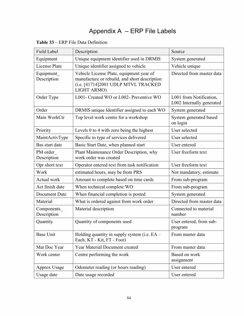
Vehicle

by

Clayton Alexander Van Volkenburg

A thesis submitted in conformity with the requirements for the degree of Master of Applied Science

Department of Mechanical and Industrial Engineering University of Toronto

© Copyright by Clayton Alexander Van Volkenburg 2014

ii

Geographic Effects on Vehicle Reliability: Developing

Proportional Hazards Models for a Deployable Military Vehicle

Clayton Alexander Van Volkenburg

Master of Applied Science

Department of Mechanical and Industrial Engineering

University of Toronto

2014

Abstract

Unlike many industries that have their equipment in one location with consistent usage patterns,

armies move their vehicles between different geographic locations with varying environmental,

and usage conditions. This creates interesting conditions for study, as those geographic changes

can be studied to detect their effect on system reliability.

Unfortunately, this is not being fully exploited, due in part to the poor capture and storage of

information, a problem faced by many operators of maintenance databases.

This thesis develops a method to characterize failure data contained in a maintenance database

using a standardized naming system, and applies a proportional hazards model for each

geographic location using covariates to represent the conditions.

In addition to understanding how a system has performed, the proportional hazards model will

allow geographic location factors to be used in predicting system reliability and spares parts

requirements in a new location.

iii

Acknowledgments

I would like to thank the members of the Centre for Maintenance Optimization and Reliability

Engineering (C-MORE) at the University of Toronto, especially the guidance and assistance of

the core staff: Professor Andrew Jardine, for allowing me to join the lab and pursue this work;

Dr. Dragan Banjevic, for always seeking a little bit more; Neil Montgomery, for his direction

and assistance optimizing EXAKT and his understanding of how the system works in the

background; and Dr. Elizabeth Thompson, for her administrative support and coffee.

I am also grateful for the assistance and support of many members of the TLAV project, and

DGLEPM; they provided a sounding board and gave clear answers to a number of problems I

encountered while cleaning the data used in this thesis. I especially would like to thank Mike

Rondeau and Frank Jutras; their intimate knowledge of the system, along with their willingness

to help, was appreciated.

Finally, I would like to thank my wife Jen, daughters Sophie, Lilian and Leia, and son Colin for

their support and more importantly their smiles.

iv

Table of Contents

Acknowledgments ......................................................................................................................... iii

Table of Contents ............................................................................................................................ iv

List of Tables .................................................................................................................................. ix

List of Plates ..................................................................................................................................xii

List of Figures .............................................................................................................................. xiii

List of Appendices ........................................................................................................................ xiv

List of Acronyms and Abbreviations ............................................................................................. xv

Chapter 1 Introduction ..................................................................................................................... 1

1.1 Overview.............................................................................................................................. 1

1.2 Army .................................................................................................................................... 1

1.3 Data Management Systems ................................................................................................. 1

1.3.1 DRMIS Data ............................................................................................................ 2

1.4 Vehicle System .................................................................................................................... 3

1.4.1 M113 History ........................................................................................................... 3

1.5 Research Motivation ............................................................................................................ 6

1.5.1 Main Research Objective ......................................................................................... 6

1.5.2 Secondary Research Objective ................................................................................ 7

1.6 Thesis Structure ................................................................................................................... 7

Chapter 2 Maintenance Processes ................................................................................................... 8

2.1 Canadian Army Maintenance .............................................................................................. 8

2.2 Spectrometric Oil Analysis Program (SOAP) ................................................................... 11

2.3 Generalized Maintenance Process ..................................................................................... 12

2.4 Data Capture ...................................................................................................................... 14

2.5 Preventive Maintenance..................................................................................................... 14

2.5.1 Definition ............................................................................................................... 14

v

2.5.2 Preventive Maintenance Themes ........................................................................... 16

2.5.3 Industry Differences .............................................................................................. 16

2.5.4 Lowest Operating Cost and Least Possible Downtime.......................................... 16

2.5.5 Refined Preventive Maintenance Statement .......................................................... 17

2.5.6 TLAV Preventive Maintenance Policy Review .................................................... 18

Chapter 3 Data Synthesis ............................................................................................................... 19

3.1 The Information Pyramid .................................................................................................. 19

3.2 Sources of Data .................................................................................................................. 20

3.3 The TLAV CMMS/ERP Dilemma .................................................................................... 21

3.3.1 Lack of Failure Mode or Failure Cause ................................................................. 22

3.3.2 Lack of Clear Dates ............................................................................................... 24

3.3.3 Freeform Text ........................................................................................................ 24

3.3.4 Incomplete Component Identification ................................................................... 25

3.3.5 Poor recording of usage data ................................................................................. 25

3.4 Remedies............................................................................................................................ 26

3.4.1 Component Identification ...................................................................................... 26

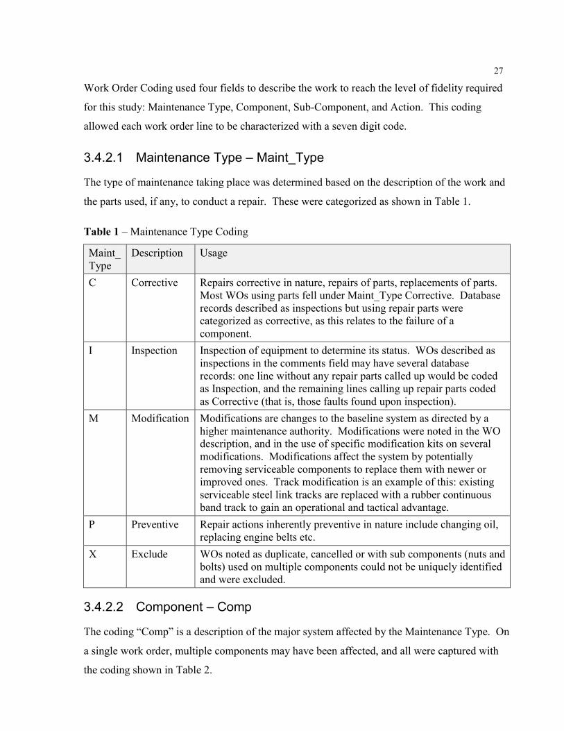
3.4.2 Work Order Coding ............................................................................................... 26

3.4.3 Vehicle Usage Calculation .................................................................................... 33

3.5 DIKW Conclusions ............................................................................................................ 34

Chapter 4 Operating Condition Effects ......................................................................................... 35

4.1 Vehicle Usage .................................................................................................................... 35

4.2 Environmental Conditions ................................................................................................. 36

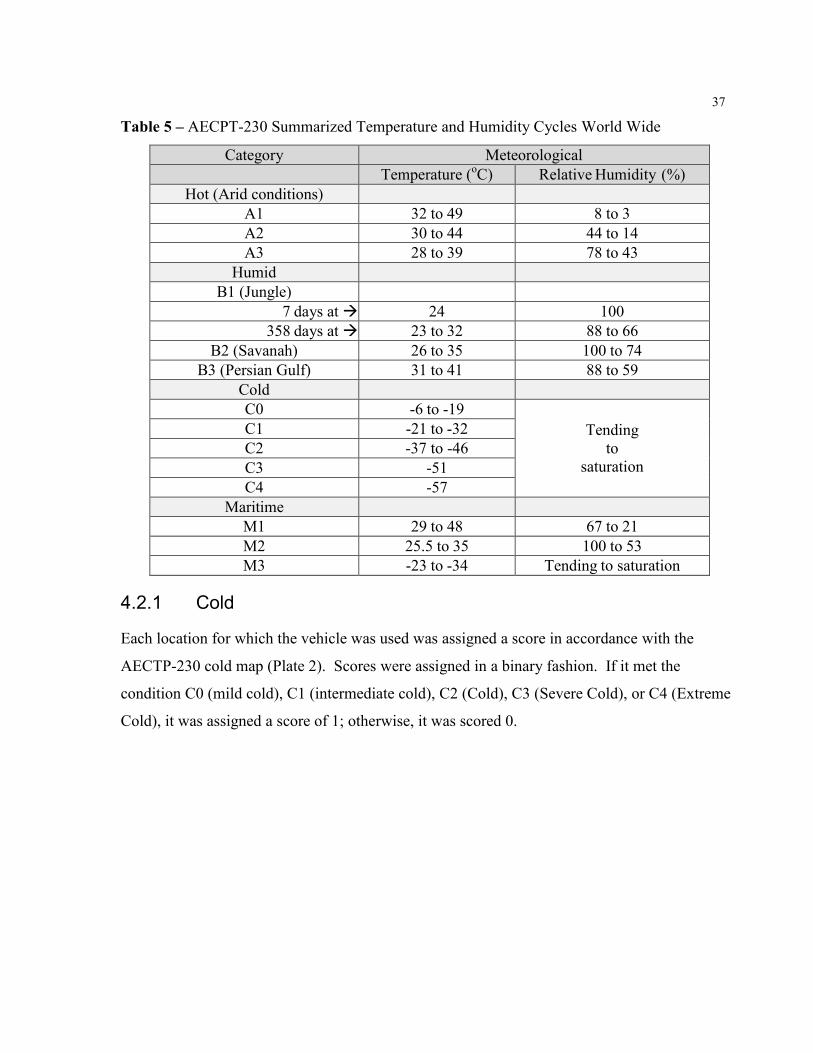
4.2.1 Cold........................................................................................................................ 37

4.2.2 Hot ......................................................................................................................... 38

4.2.3 Hot–Humid ............................................................................................................ 40

4.3 Geographic Conditions ...................................................................................................... 40

vi

4.4 Operating Conditions ......................................................................................................... 41

4.4.1 Operator Experience .............................................................................................. 41

4.4.2 Idling Time ............................................................................................................ 41

4.4.3 Add-on-Armour ..................................................................................................... 41

4.5 Additional Future Conditions ............................................................................................ 41

4.5.1 Wet or Dusty .......................................................................................................... 41

4.5.2 Extreme Cold ......................................................................................................... 42

4.5.3 Stagnation .............................................................................................................. 42

4.5.4 Rocks/Unprepared Surfaces................................................................................... 42

4.5.5 Storage ................................................................................................................... 42

4.5.6 Mountainous Terrain ............................................................................................. 42

4.5.7 Maritime Environment........................................................................................... 43

4.5.8 General Condition Covariate Summary................................................................. 43

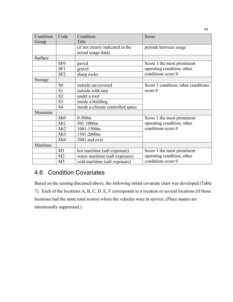
4.6 Condition Covariates ......................................................................................................... 44

4.7 SOAP Analysis .................................................................................................................. 45

Chapter 5 Proportional Hazards Model Development................................................................... 46

5.1 EXAKT .............................................................................................................................. 46

5.2 Data Input .......................................................................................................................... 46

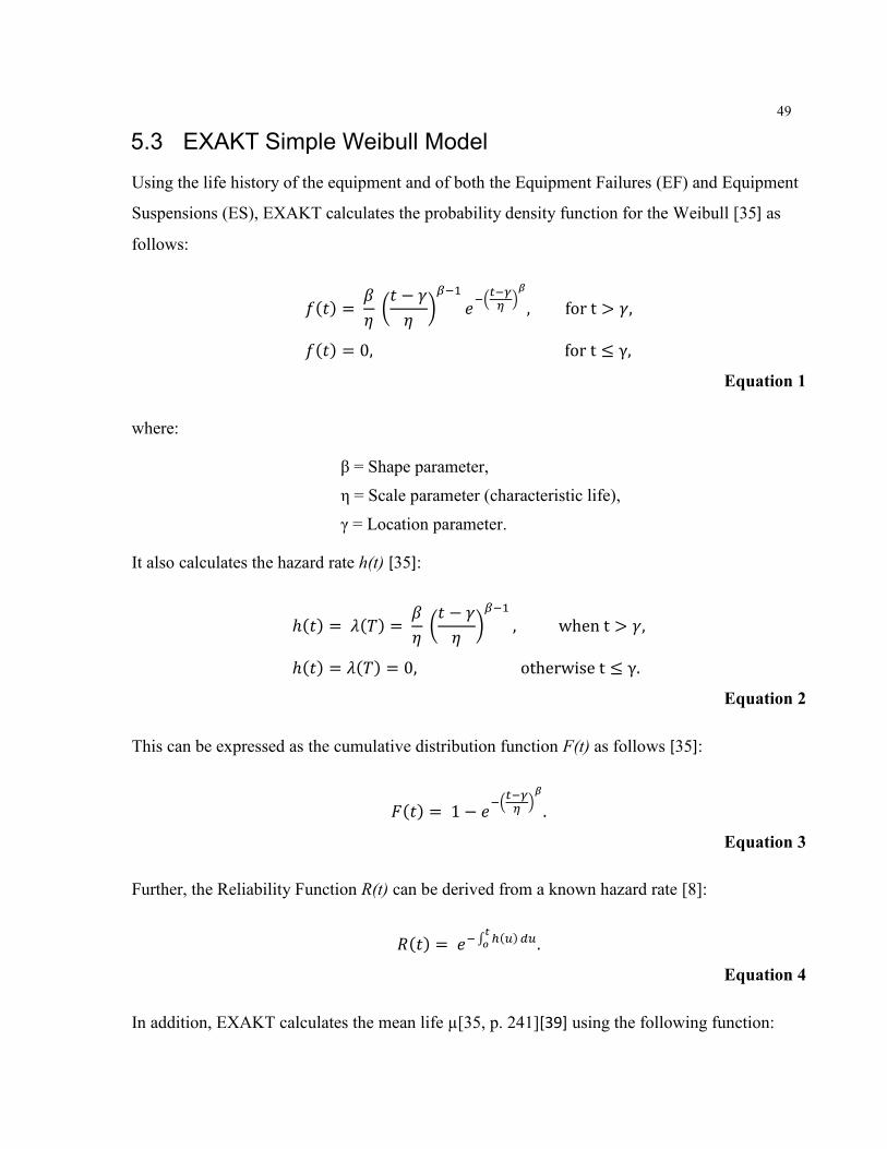
5.3 EXAKT Simple Weibull Model ........................................................................................ 49

5.3.1 EXAKT Proportional Hazards Model ................................................................... 51

5.4 Data Processing: Moving Up the DIKW Pyramid ............................................................ 53

5.4.1 Data to Information................................................................................................ 53

5.4.2 Transmissions ........................................................................................................ 53

5.4.3 Engines .................................................................................................................. 65

5.4.4 Suspension Systems ............................................................................................... 70

5.5 Summary Table .................................................................................................................. 71

vii

5.6 Information to Knowledge ................................................................................................. 72

5.7 Data to Wisdom ................................................................................................................. 73

5.7.1 General Formulation .............................................................................................. 73

5.7.2 Software Integration .............................................................................................. 75

Chapter 6 Conclusion .................................................................................................................... 77

6.1 Results ............................................................................................................................... 77

6.2 Data .................................................................................................................................... 77

6.3 Reaching the Peak of DIKW ............................................................................................. 77

6.4 Additional Data Manipulation ........................................................................................... 78

Chapter 7 Future Work .................................................................................................................. 79

7.1 ERP Data Characterization ................................................................................................ 79

7.2 Covariate Development ..................................................................................................... 79

7.3 Covariate Integration ......................................................................................................... 79

References...................................................................................................................................... 80

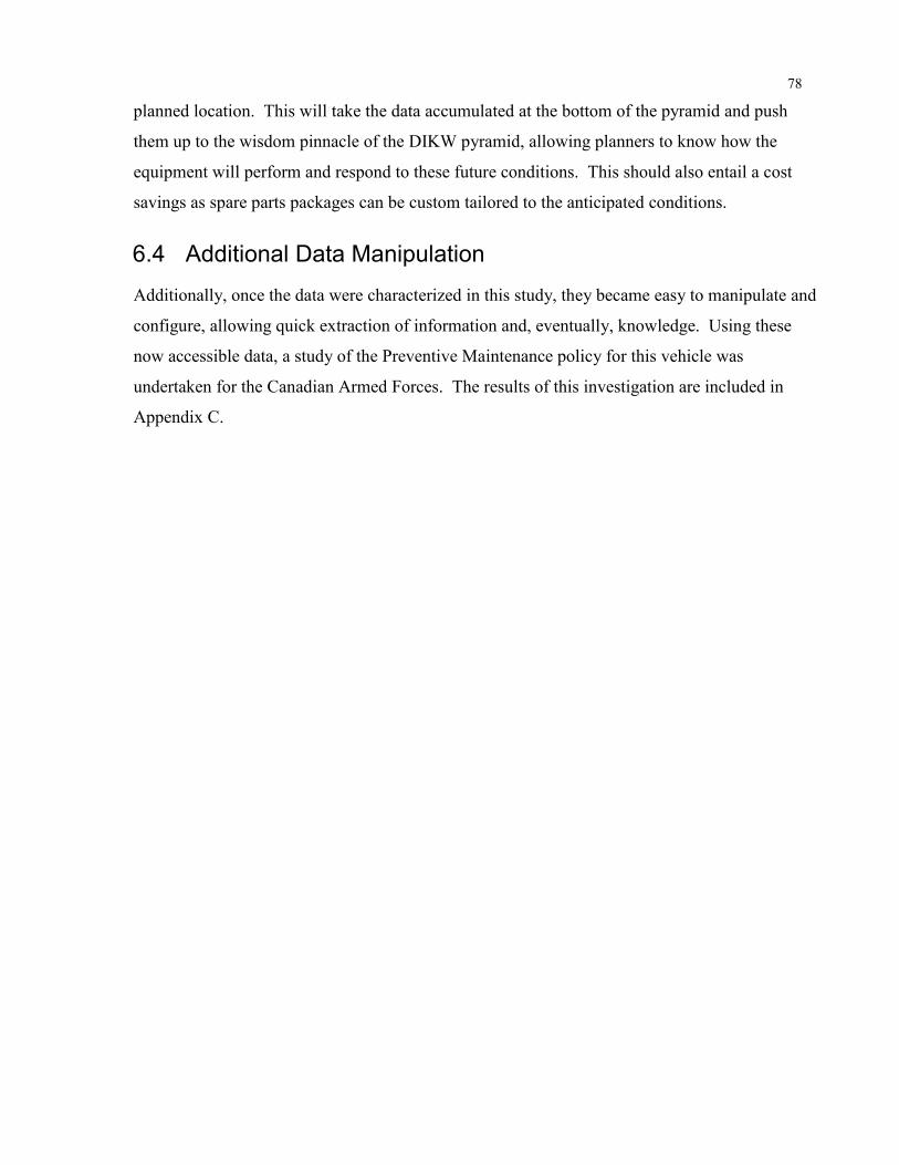
Appendix A – ERP File Labels .................................................................................................. 84

Appendix B – CMMS File Labels ............................................................................................. 85

Appendix C – Preventive Maintenance Analysis....................................................................... 86

C.1 Data .................................................................................................................................... 86

C.2 Existing Inspection Regime ............................................................................................... 86

C.3 Data Compilation ............................................................................................................... 86

C.4 Pareto Analysis .................................................................................................................. 87

C.5 Pareto Comparison to Inspection Items ............................................................................. 88

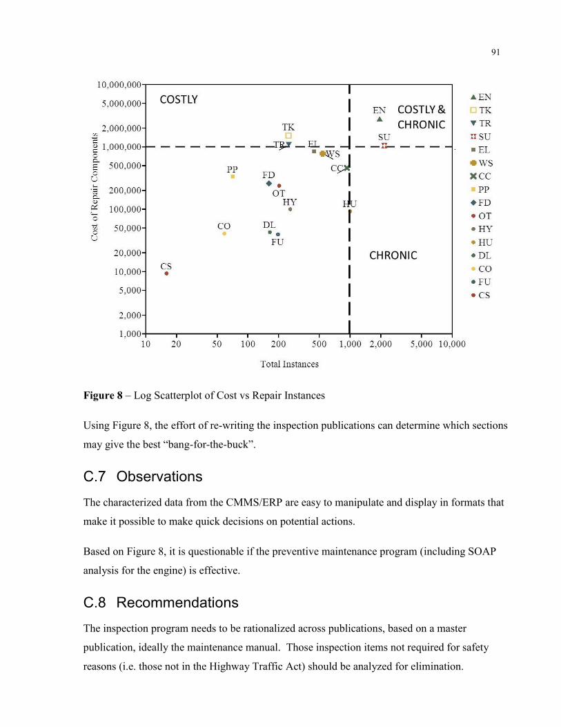
C.6 Moving Beyond Pareto ...................................................................................................... 89

C.7 Observations ...................................................................................................................... 91

C.8 Recommendations.............................................................................................................. 91

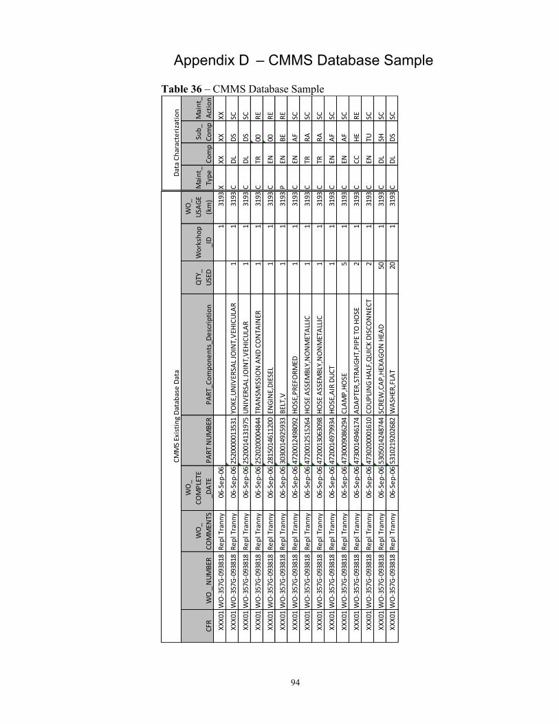
Appendix D – CMMS Database Sample .................................................................................... 94

viii

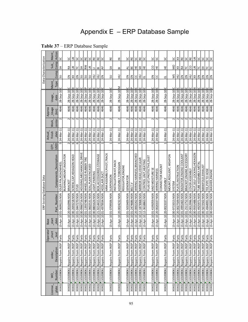
Appendix E – ERP Database Sample ........................................................................................ 95

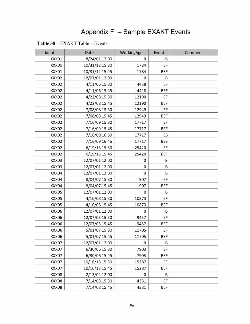
Appendix F – Sample EXAKT Events ...................................................................................... 96

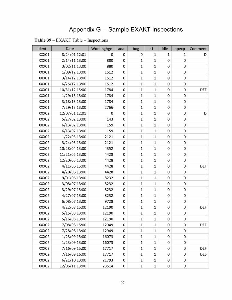
Appendix G – Sample EXAKT Inspections............................................................................... 97

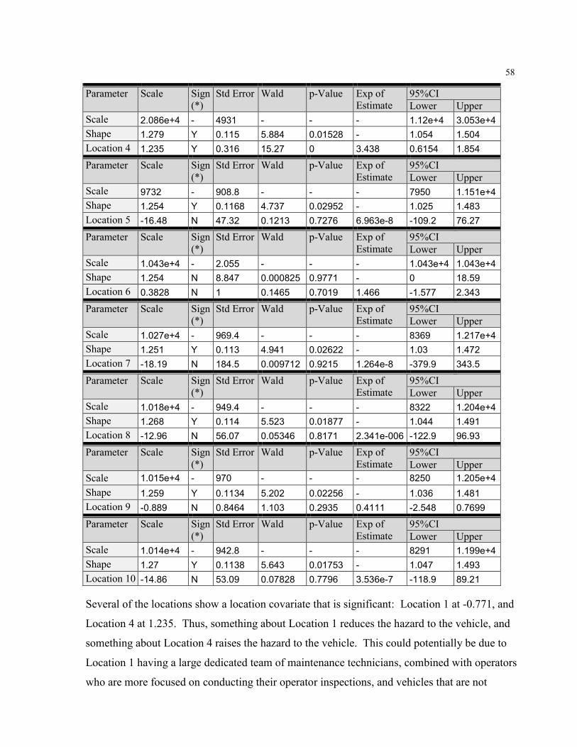
Appendix H – Transmission Location Covariate Reduction...................................................... 98

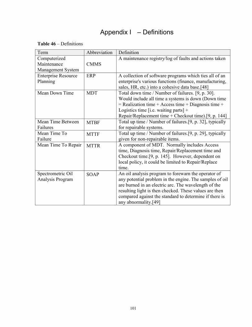
Appendix I – Definitions ........................................................................................................ 101

ix

List of Tables

Table 1 – Maintenance Type Coding........................................................................................... 27

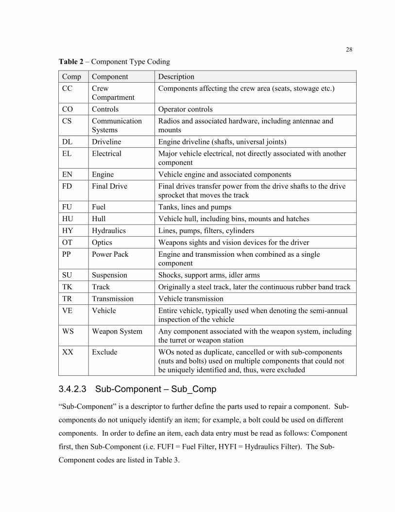
Table 2 – Component Type Coding............................................................................................. 28

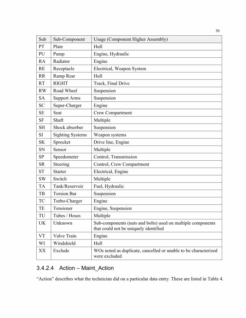
Table 3 – Sub-Component Type Coding ..................................................................................... 29

Table 4 – Maintenance Action Coding ........................................................................................ 31

Table 5 – AECPT-230 Summarized Temperature and Humidity Cycles World Wide ............... 37

Table 6 – Covariate Selection Chart ............................................................................................ 43

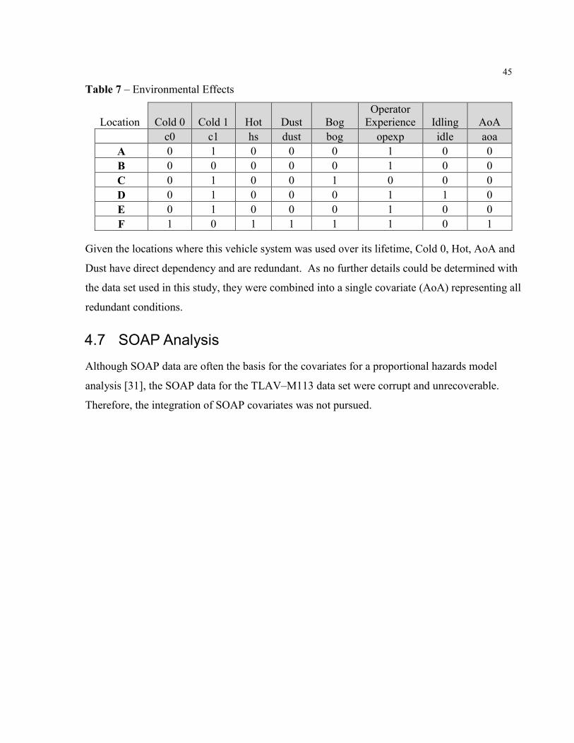
Table 7 – Environmental Effects ................................................................................................. 45

Table 8 – Event Precedence ......................................................................................................... 48

Table 9 – EXAKT Output Definitions ........................................................................................ 51

Table 10 – Weibull Shape Parameter .......................................................................................... 51

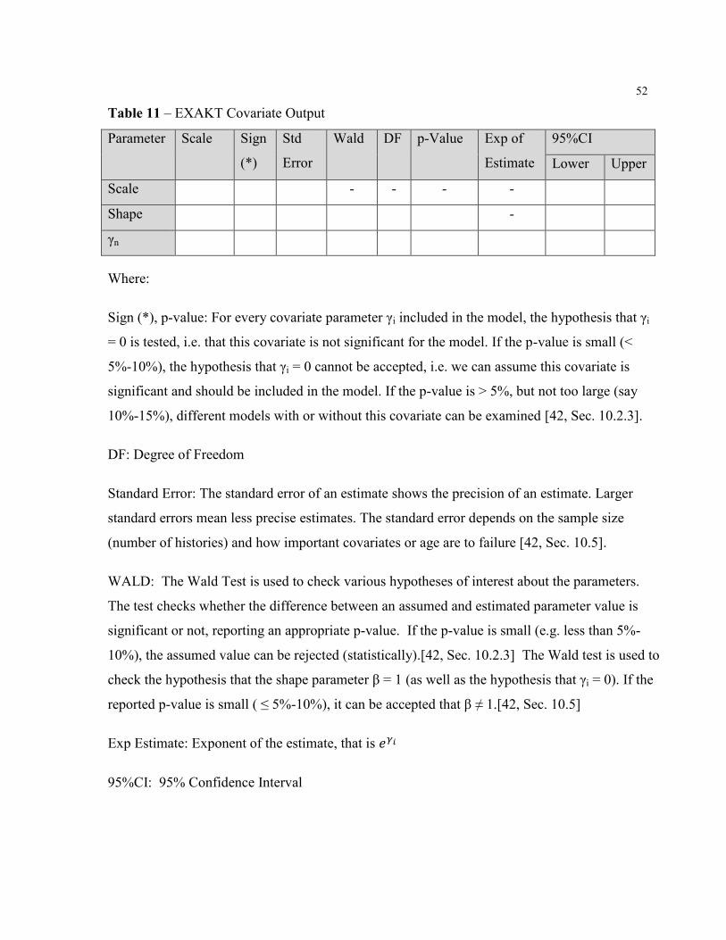
Table 11 – EXAKT Covariate Output ......................................................................................... 52

Table 12 – Transmission Weibull Distribution ........................................................................... 54

Table 13 – Location Covariates ................................................................................................... 55

Table 14 – Transmission Locational Covariates ......................................................................... 55

Table 15 – Transmission Locational Covariates – first reduction step ....................................... 56

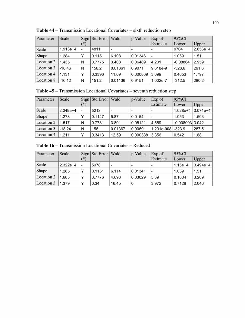
Table 16 – Transmission Locational Covariates – Reduced ....................................................... 56

Table 17 – Transmission Individual Location Analysis .............................................................. 57

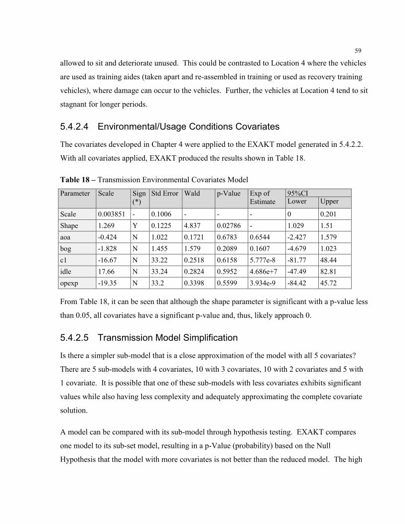
Table 18 – Transmission Environmental Covariates Model ....................................................... 59

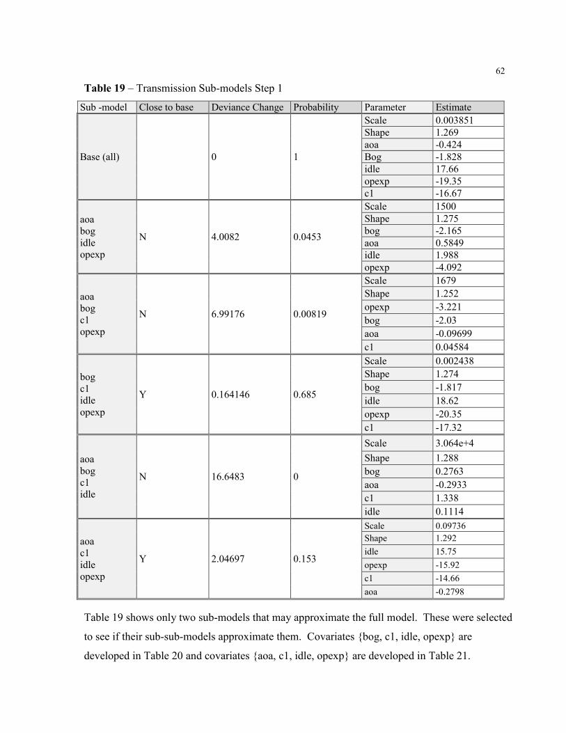
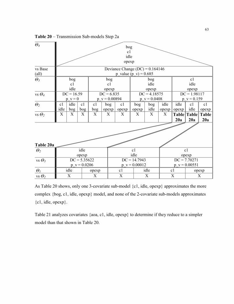
Table 19 – Transmission Sub-models Step 1 .............................................................................. 62

Table 20 – Transmission Sub-models Step 2a ............................................................................. 63

x

Table 21 – Transmission Sub-models Step 2b ............................................................................ 64

Table 22 – Transmission Three Covariate Sub-model ................................................................ 64

Table 23 – Engine Weibull Distribution ...................................................................................... 65

Table 24 – Engine, shape parameter = 1 ..................................................................................... 65

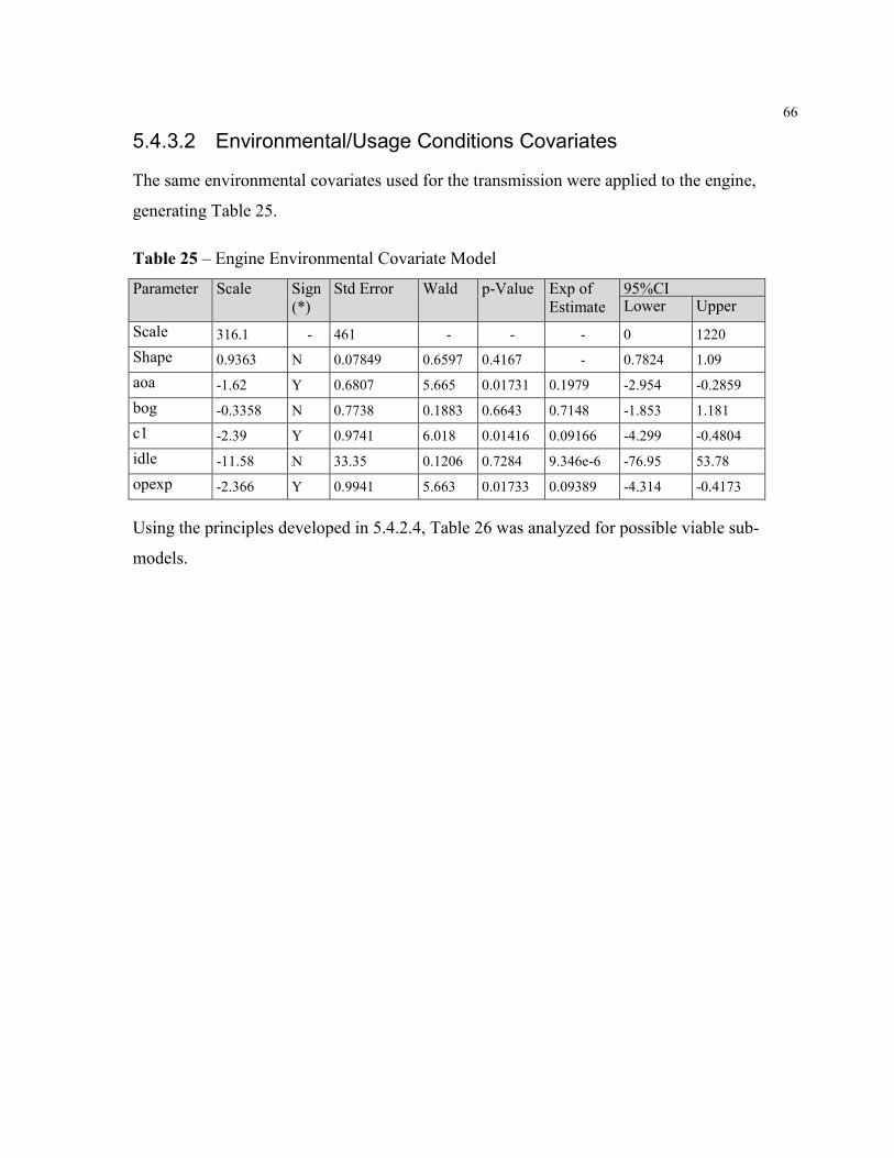
Table 25 – Engine Environmental Covariate Model ................................................................... 66

Table 26 – Engine Sub-model Step 1 .......................................................................................... 67

Table 27 – Engine Sub-models Step 2a ....................................................................................... 68

Table 28 – Engine Sub-models Step 2b ....................................................................................... 69

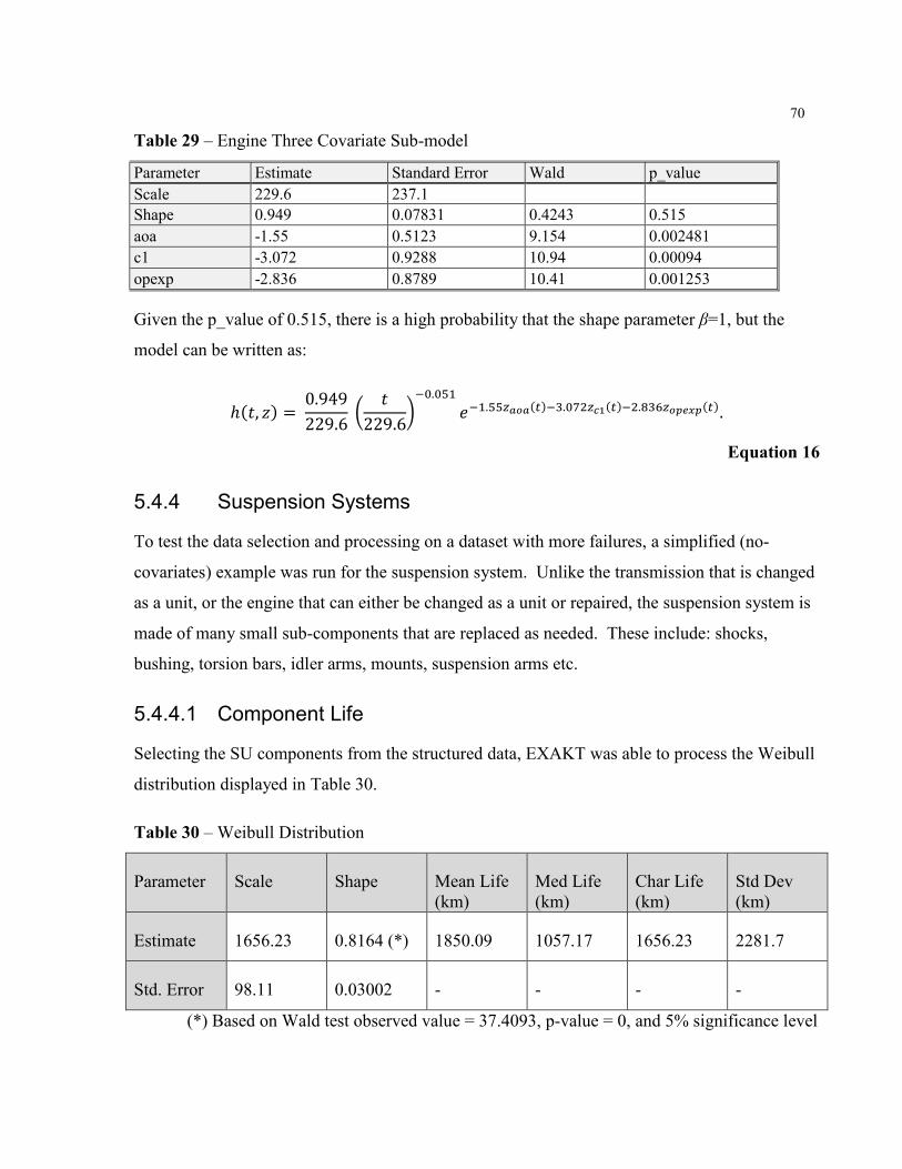
Table 29 – Engine Three Covariate Sub-model .......................................................................... 70

Table 30 – Weibull Distribution .................................................................................................. 70

Table 31 – Summary of Hazard Functions for the M113 ............................................................ 72

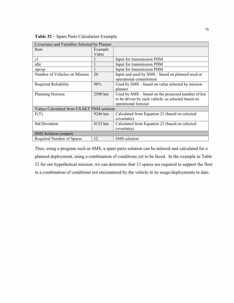
Table 32 – Spare Parts Calculation Example .............................................................................. 76

Table 33 – ERP File Data Definition ........................................................................................... 84

Table 34 – CMMS File Data Definition ...................................................................................... 85

Table 35 – TLAV Maintenance Manual and 1136 Comparison Chart ....................................... 93

Table 36 – CMMS Database Sample .......................................................................................... 94

Table 37 – ERP Database Sample ............................................................................................... 95

Table 38 – EXAKT Table – Events ............................................................................................. 96

Table 39 – EXAKT Table – Inspections ..................................................................................... 97

Table 40 – Transmission Locational Covariates – second reduction step ................................... 98

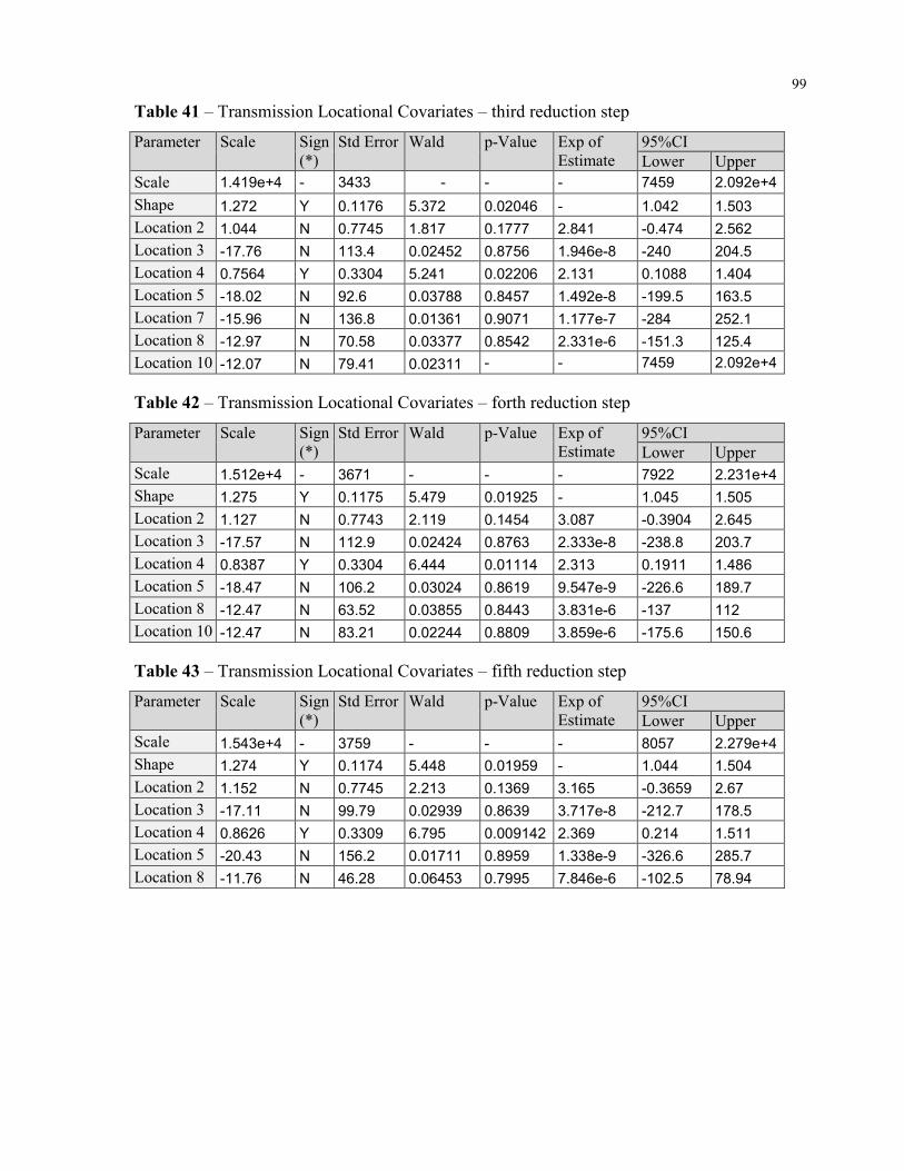
Table 41 – Transmission Locational Covariates – third reduction step ...................................... 99

xi

Table 42 – Transmission Locational Covariates – forth reduction step ...................................... 99

Table 43 – Transmission Locational Covariates – fifth reduction step ....................................... 99

Table 44 – Transmission Locational Covariates – sixth reduction step .................................... 100

Table 45 – Transmission Locational Covariates – seventh reduction step ................................ 100

Table 46 – Definitions ............................................................................................................... 101

xii

List of Plates

Plate 1 – TLAV - M113A3 ............................................................................................................ 5

Plate 2 – Climatic Categories Map: Cold [32] ............................................................................ 38

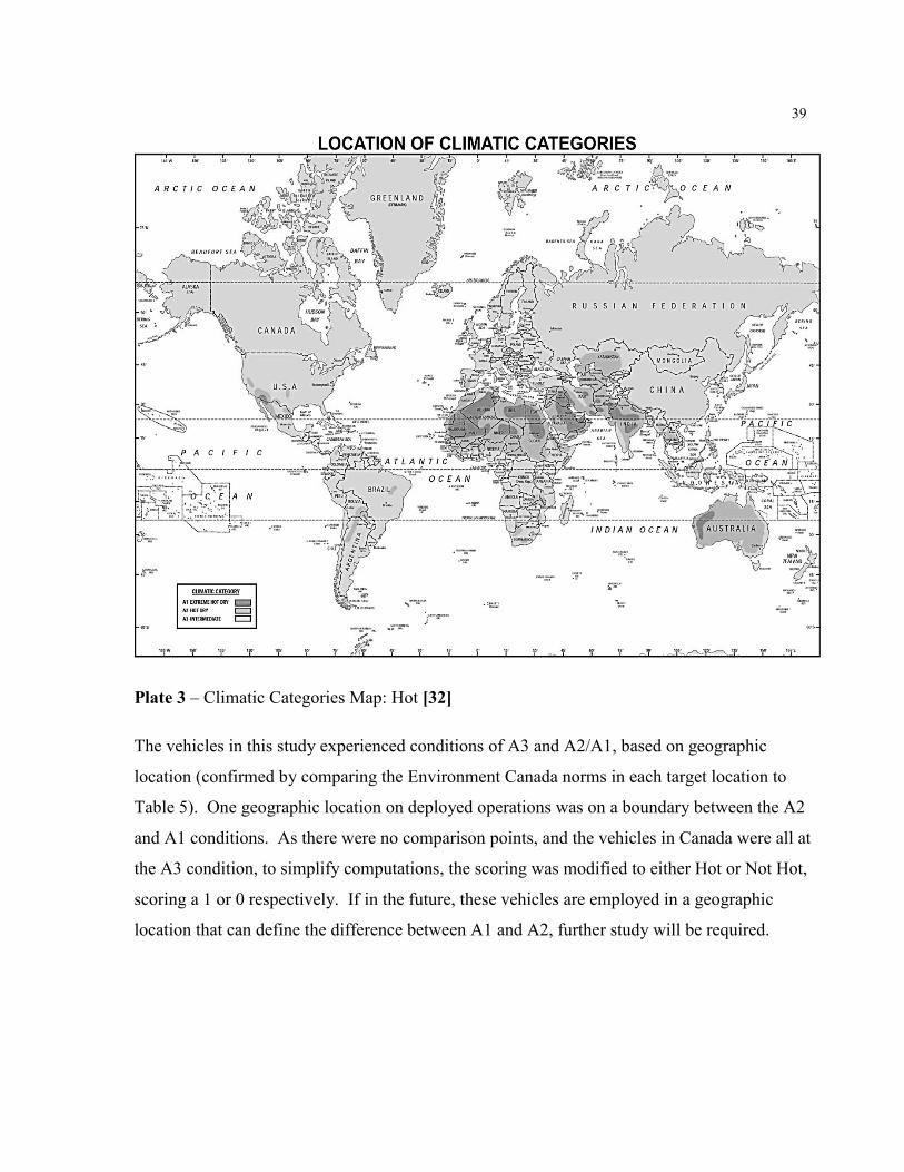
Plate 3 – Climatic Categories Map: Hot [32] .............................................................................. 39

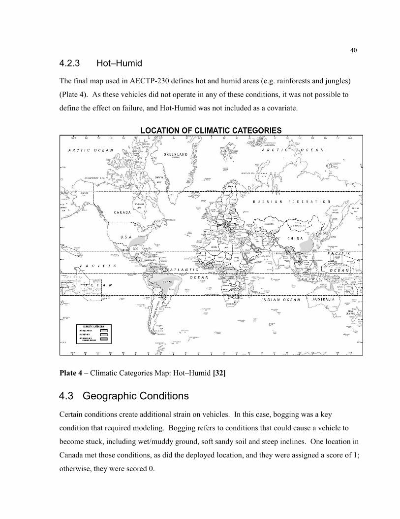
Plate 4 – Climatic Categories Map: Hot–Humid [32] ................................................................. 40

Plate 5 – Log Scatterplot Showing Limit Values from Knights .................................................. 90

xiii

List of Figures

Figure 1 – Preventive Maintenance Work Flow .......................................................................... 12

Figure 2 – Corrective Maintenance Work Flow .......................................................................... 13

Figure 3 – DIKW Pyramid .......................................................................................................... 19

Figure 4 – Example EXAKT Equipment Component Life History ............................................ 48

Figure 5 – Repair Cost Pareto Histogram .................................................................................... 87

Figure 6 – Operator Inspections vs Costs of Repair .................................................................... 88

Figure 7 – Operator Inspections vs Number of Repair Items ...................................................... 89

Figure 8 – Log Scatterplot of Cost vs Repair Instances .............................................................. 91

xiv

List of Appendices

Appendix A – ERP File Labels .................................................................................................. 84

Appendix B – CMMS File Labels ............................................................................................. 85

Appendix C – Preventive Maintenance Analysis....................................................................... 86

Annex 1 to Appendix C ............................................................................................................ 93

Appendix D – CMMS Database Sample .................................................................................... 94

Appendix E – ERP Database Sample ........................................................................................ 95

Appendix F – Sample EXAKT Events ...................................................................................... 96

Appendix G – Sample EXAKT Inspections............................................................................... 97

Appendix H – Transmission Location Covariate Reduction...................................................... 98

Appendix I – Definitions ........................................................................................................ 101

xv

List of Acronyms and Abbreviations

Abbreviation Meaning

AECTP Allied Environmental Conditions and Test Publication

AoA Add on Armour

APC Armoured Personnel Carrier

ARVL Armoured Recovery Vehicle Light

CAF Canadian Armed Forces

CBM Condition Based Monitoring

CF Canadian Forces

CFR Canadian Forces Registration

CM Corrective Maintenance

CMMS Computerized Maintenance Management System (see Appendix I –

Definitions)

C-MORE The Centre for Maintenance Optimization and Reliability Engineering

Cu Copper

DIKW Data-Information-Knowledge-Wisdom

DND Department of National Defence (Canada)

DoD Department of Defense (United States of America)

DRMIS Defence Resource Management Information System

Eqpt Equipment

ERN Equipment Registration Number

ERP Enterprise Resource Planning (see Appendix I – Definitions)

EXAKT The name of a Condition Based Monitoring software

Fe Iron

FMS Fleet Management System

FOV Family of Vehicles

Ident Identity

km Kilometre

LEMS Land Engineering Maintenance System

M113 An armoured vehicle

MRT Mobile Repair Team

MTBF Mean Time Between Failure (see Appendix I – Definitions)

MTBR Mean Time Between Replacements

MTTF Mean Time To Failure (see Appendix I – Definitions)

MTTR Mean Time To Repair (see Appendix I – Definitions)

xvi

MTV Mobile Tactical Vehicle

MTVL Mobile Tactical Vehicle Light

NATO North Atlantic Treaty Organization

NSN NATO Stock Number

OEM Original Equipment Manufacturer

PHM Proportional Hazards Model

PLANNEx PLANN Expert – a CMMS program

PM Preventive Maintenance

ppm Parts per million

RWS Remote Weapon Station

SAP A brand name of an ERP

SMS Spares Management Software

SOAP Spectrometric Oil Analysis Program

TLAV Tracked Light Armoured Vehicle

WO Work Order

1

Chapter 1

Introduction

1.1 Overview

The Canadian Armed Forces deploys vehicles, equipment, supplies and personnel on a variety

of operational missions, both domestically and internationally. Additionally, these same

equipment and vehicle types are used for a variety of training scenarios, from individual driver

training to large formation training exercises. In these deployments the vehicles experience a

wide variety of operating conditions and scenarios over their lifetime.

This thesis introduces a system to characterize data in maintenance databases and a method of

developing a proportional hazards model (PHM) to model the effects of various environmental

conditions on those vehicles used in the various geographic locations.

1.2 Army

The Canadian Army, Canada’s land element, along with the Royal Canadian Navy, Royal

Canadian Air Force and others, form the Canadian Armed Forces(CAF) (formerly the Canadian

Forces(CF)), which is supported by the Department of National Defence. The Canadian Army

is equipped with a variety of vehicles and systems that are employed by units to conduct training

and operations in a variety of environments with varying intensities. The equipment is

supported with spare parts provided from a multi-tiered supply chain, with maintenance

technician support from uniformed army mechanics, Department of National Defence civilian

employees, as well as internal and external contractors.

1.3 Data Management Systems

In order to support maintenance operations the DND uses a software solution to provide the

following[1]:

1. a centralized repository for land technical equipment data, costs and technical information;

2. storage of land technical equipment preventive maintenance plans, and the generation and

tracking of preventive maintenance work;

2

3. the management tools for processing control documentation, resource management, and

interfacing with other Canadian Forces systems; and

4. the ability to collate information to measure equipment and workshop performance.

For a number of years, the Canadian Army used a Computerized Maintenance Management

System (CMMS) called PLANN Expert, which ran locally on workshop computers and was

updated to a central server manually. Starting in the late 2000s, the Canadian Armed Forces and

the Department of National Defence began conversion to an integrated Enterprise Resource

Planning (ERP) software solution based on the SAP product known as the Defence Resource

Management Information System (DRMIS). DRMIS combines finance, task notification, work-

order documentation, inventory control, purchasing and other processes (modules) into a Forces

wide system.

The collection of data into DRMIS for the Canadian Armed Forces is an on-going process,

similar to the collection process undertaken by many industries and government organizations

around the world. PLANN Expert was the first real CMMS used by the Canadian Army; in

effect, the data were stored on “electronic paper” in a manner similar to how they were filed

prior to computerization. On some levels, the “electronic paper” data records are treated like

paper records. The information is kept closely bound and filed in discrete locations (similar to

filing papers in a cabinet) where it accumulates, ultimately becoming hard to process or access

in a meaningful manner. The ERP system with its interlinked data seeks to move away from

this model; in this system, the data are accessible and configurable, allowing decisions to be

made in a timely manner based on the stored data. Unfortunately, with the migration from the

PLANN Expert CMMS to the DRMIS ERP, some of the same attitudes towards and

expectations of the electronic data have remained. The system may not be used to its full

potential; indeed, in some instances, the users entering the data are treating the inputs simply as

data required to feed the system in order to get to the next step or screen.

1.3.1 DRMIS Data

DRMIS was implemented on a rollout, location-by-location across the Canadian Army. As

locations went “live,” data were imported from the previous system, and technicians began

3

working in the SAP DRMIS program. As such, to cover the full period of service life of

equipment, this thesis has had to analyze data from both PLANN Expert and DRMIS and

synthesis them into a single database. Thus, a complete data record for most systems contains

both older PLANN Expert data and newer DRMIS entries.

DRMIS contains multiple modules and data sources. Some data sources are resident within

DRMIS, some come from user inputs, others are tombstone data (established non-changing data

such as vehicle identification numbers), and still others are inputs from other database systems.

The entire DRMIS database is too complex and large to analyze and contains data not relevant

to the study of system reliability. The data used for this thesis comprise an extract from the SAP

system concerning vehicle maintenance on a specific fleet output to a Microsoft Excel file. The

format for the data is located in the appendices: DRMIS (ERP) data format appears in Appendix

A, PLANN Expert (CMMS) in Appendix B. In each of these extracts, the data were based on

unique work order numbers assigned to specific pieces of equipment at specific times.

1.4 Vehicle System

Although the Canadian Armed Forces has a variety of vehicles, ships and planes, this thesis has

selected the Tracked Light Armoured Vehicle (TLAV)(also known as the M113A3) for study.

The TLAV has been used in various locations and experiences a wide variety of usage patterns

and environmental conditions. It has been used in high intensity operations in hot dry locations

and during training in muddy, wet and cold conditions. Certain TLAVs have also sat for

extended periods either while the assigned users were deployed on Operations, or while the

vehicle was in transit to a new location or being held in reserve. This non-homogeneous

environmental and usage history can be complex. Specifically, the complex usage history

complicates the ERP’s ability to produce information that the fleet managers can use to modify

or improve the existing maintenance processes or practices.

1.4.1 M113 History

The current TLAV Family of Vehicles (FOV) is based on the M113 armoured vehicle platform

developed by the United States of America and introduced into service in the early 1960s.

Canada began acquiring the M113 in the 1960s; over several years, Canadian Army units were

4

equipped with these vehicles. Subsequent to purchase, Canada upgraded and converted to the

M113A2 variant which featured some performance upgrades as well as externally mounted fuel

tanks on the rear sponsons.

Primarily purchased as an Armoured Personnel Carrier (APC) vehicle for the infantry,

command and support variants based on the same chassis were also acquired. In addition to the

APC, the M113A2 family of vehicles included: a command version, the M577 Command Post;

a supply vehicle, the M548 Cargo Carrier; the Air Defence Anti-Tank System (ADATS); the

Tube-launched optically wire-guided Under Armour (TUA); a combat engineering vehicle with

dozer blade; the M113 Fitter, a Mobile Repair Team (MRT) maintenance vehicle; the Armoured

Recovery Vehicle Light (ARVL), a maintenance recovery variant; the Damaged Airfield

Reconnaissance Explosive Ordnance Disposal (DAREOD); and the Improved Land-Mine

Detection System (ILDS).

The M113A2 saw extensive service in Canada both as a training vehicle and for domestic and

international operations and was used heavily by 4 Canadian Mechanized Brigade Group

(4CMBG) while deployed to Germany during the Cold War. The M113 is widely used

throughout the world with production numbers in excess of 80,000 over 40 plus years of

production, making it one of the most common armoured vehicle platforms in service.[2]

Over several years in the late 1990s and 2000s, the Armoured Personnel Carrier Life Extension

project developed and produced several hundred new upgraded systems called TLAVs which

were upgraded from the M113A2 chassis, with the remainder of the M113A2s declared surplus

and removed from inventory.

This mid-life reset of the M113A2 to the TLAV resulted in considerable changes to the fleet

with significant performance upgrades. With the TLAV, two hull designs were implemented;

the M113A3 hull based on the M113A2, and the Mobile Tactical Vehicle (MTV) hull which

took existing M113A2 hulls, cut them and extended them to fit an additional road wheel,

allowing increased suspension and carrying capacity.

For both the M113A3 and the MTV, upgrades were made to the drive-train, armour protection,

operator systems, weapon systems and vehicle electronics. The vehicle was converted from the

5

existing tiller bar operated steering system to a steering yoke system, much like a regular car.

The existing diesel engine was replaced by an up-powered diesel engine with a modern

electronic management system. At the same time, the fleet began conversion to a Soucy

International Inc. continuous rubber band track, replacing the existing Diehl linked steel track.

The combined upgrades resulted in increased vehicle performance and comfort. In addition to

improving the performance, the upgrades were intended to improve system reliability. To aid in

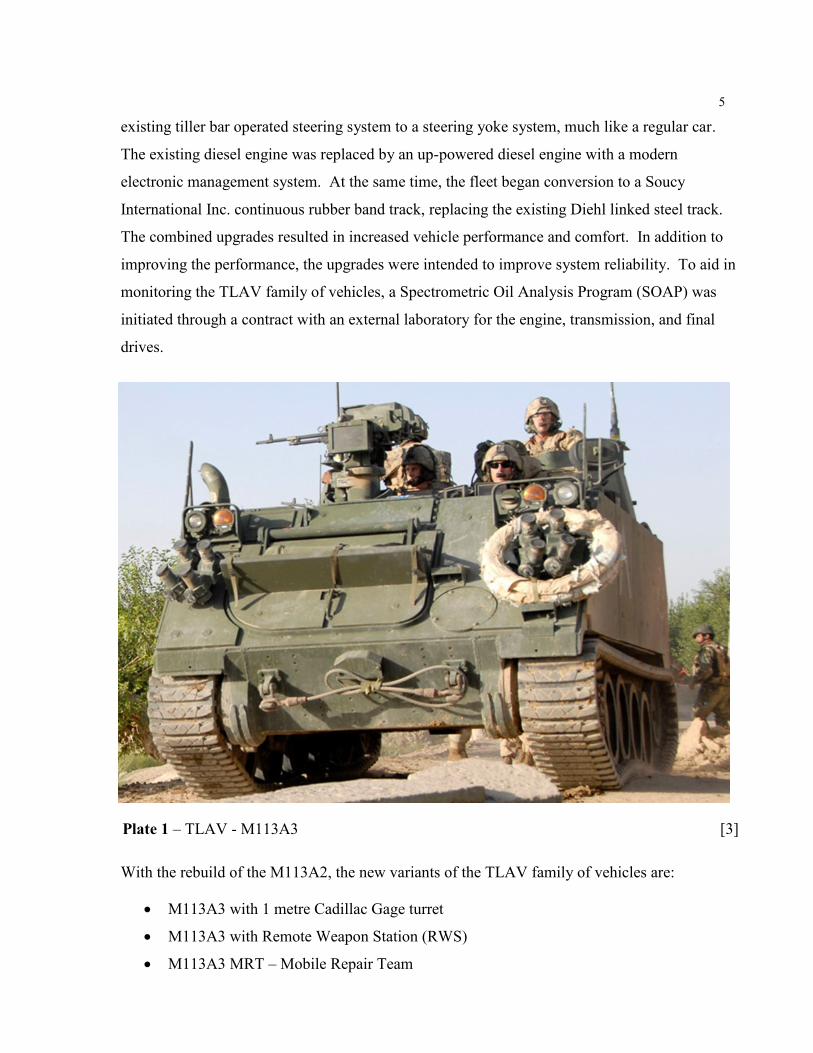
monitoring the TLAV family of vehicles, a Spectrometric Oil Analysis Program (SOAP) was

initiated through a contract with an external laboratory for the engine, transmission, and final

drives.

[3]

With the rebuild of the M113A2, the new variants of the TLAV family of vehicles are:

M113A3 with 1 metre Cadillac Gage turret

M113A3 with Remote Weapon Station (RWS)

M113A3 MRT – Mobile Repair Team

Plate 1 – TLAV - M113A3

6

M577A3 Command Post

MTVR – Mobile Tactical Vehicle Recovery

MTVE – Mobile Tactical Vehicle Engineer

MTVL with turret

MTVL with RWS

MTVF – Mobile Tactical Vehicle Fitter (Mobile Repair Team with RWS)

MTVA – Mobile Tactical Vehicle Ambulance

The introduction of turrets and RWS upgrades modified how the Army employed the M113A2,

as the TLAV demonstrated increased capabilities.

The introduction of the TLAV into service also happened to coincide with the operational

requirement for this type of vehicle in Afghanistan. The TLAV with the Soucy rubber track saw

considerable service in Afghanistan and among units in Canada training for deployment.

The M113A3’s recent re-fit and the long history and extensive use of this vehicle platform make

it an interesting vehicle for study and a good basis for devising a maintenance solution

applicable to other platforms.

1.5 Research Motivation

I was motivated to study the M113 as it has seen widespread use by many militaries; given its

deployment to different locations, it is a good candidate to study the environmental effects of

location on the reliability of a vehicle.

1.5.1 Main Research Objective

My main research objective was to develop a mechanism to quickly characterize locations using

a standard convention. These locations could then form the covariates influencing the

proportional hazards model for the component being studied. Further, I wanted to be able to use

this model to calculate spare parts requirements for locations with different combinations of

covariates, even for combinations the vehicle has yet to experience.

7

1.5.2 Secondary Research Objective

My secondary research objective was to develop a method to improve the structure of a

maintenance database to allow it to be quickly searched for work orders applicable to the

component under investigation.

1.6 Thesis Structure

Following the introduction, I will detail the maintenance process in Chapter 2, concentrating on

the maintenance process for the M113 in the Canadian Army inventory. This chapter also

includes a literature review of the definition and concept of preventive maintenance and offers

an alternative definition. Chapter 3 introduces the concept of taking raw unstructured data and

transforming and improving them into useful information; importantly, this chapter details a

method to characterize the data to make them quickly and efficiently searchable. Chapter 4

defines the effects of environmental factors on the vehicle and establishes a standardized

classification system. Chapter 5 develops the proportional hazards model for the transmission,

engine and suspension systems using the covariates developed in Chapter 4. I finish the main

body of the work with conclusions and suggest possible future work. The appendices contain

supporting information and tables as well as a study on the preventive maintenance program of

the M113 based on the characterized database developed in Chapter 3.

8

Chapter 2

Maintenance Processes

2.1 Canadian Army Maintenance

The Canadian Department of National Defence (DND) establishes its strategic Maintenance

Policy in a series of keystone publications. These publications, in combination with equipment

specific publications, provide direction and guidance to units holding equipment as to which

actions are to be taken to support that equipment. These publications define both what

maintenance is done and who does the maintenance. This is accomplished through a system

known as Lines and Levels of maintenance.

Levels of Maintenance are defined as “a measure of the work content, complexity or depth of a

maintenance support task” [4, Ch. 3]. There are four levels of maintenance: level one is the

lowest, indicating basic repair tasks; level four is the highest, indicating extensive maintenance

resources. In greater detail[4, p. 3]:

Level One. Generally involves preventive maintenance, fault finding and limited

corrective maintenance. Tasks are usually of limited complexity and short

duration. Examples of level one tasks include:

a. servicing and serviceability checks by both operator and technician;

b. periodic equipment inspections;

c. fault finding and preliminary diagnosis including classification of

equipment casualties;

d. preservation/de-preservation;

e. adjustments;

f. minor modifications;

g. replacement of parts or components before failure; and

h. replacement of failed parts, modules and components.

Level Two. Primarily involves intermediate corrective maintenance, typically

including:

a. replacement of components (including major assemblies) within

equipments or systems;

b. modifications;

9

c. repair to components and modules; and

d. detailed diagnostics and inspections.

Level Three. Involves more extensive and complex maintenance tasks that may

involve the use of a production line, special test equipment, and limited

manufacture. These tasks generally include:

a. adjustments and alignment of complete equipments and systems;

b. reconditioning of assemblies, equipments and systems, such as

engines, drive trains, guns, and electrical/electronic assemblies;

c. major modifications;

d. reclamation; and

e. calibration of electrical/mechanical test and diagnostic equipment.

Level Four. Involves the complete overhaul of equipment that generally

includes:

a. conducting salvage operations;

b. fabrication of parts;

c. returning an item or equipment to its original specifications, or to a

specified standard;

d. retrofit;

e. effecting mid-life improvements; and

f. extending the planned economical life of an equipment.

In conjunction with levels of maintenance, the lines of maintenance indicate the organization

performing the maintenance. Tasks are assigned to lines of maintenance considering such

factors as: time, tactical situation, tools, test equipment, mobility and repair parts. The

overriding factor is time. Lines of maintenance are divided into four lines, with the first line

being the most tactical and mobile in nature and the fourth being the most strategic. In greater

detail [4, p. 5]:

First Line. First line maintenance organizations are normally the first

maintenance organization to which the user turns. It principally performs level

one and possibly limited level two maintenance tasks. No task of more than

four (4) hours duration will normally be assigned to first line, regardless of the

10

level of maintenance involved. These resources could be augmented by

crews/operators from second line.

Second Line. The next higher maintenance organization. It principally

performs level two and limited level three maintenance tasks. It also carries

out level one technical maintenance services for those organizations without

integral maintenance support and handles overload from first line maintenance

organizations. Second line workshops have greater carrying capacities,

availability of repair tooling and decreased proximity to the enemy compared to

first line workshops. Time is again the overriding factor with the task duration

limits set at 12 hours for mobile repair team (MRT) in-situ repairs and 24

hours at the main workshop location.

Third Line. Third line maintenance organizations have limited mobility and

perform more specialized and/or more complex maintenance tasks. They

perform level three tasks as well as lesser level tasks as a back-up for the

formations/units it supports. In this regard, they may provide level one

maintenance services to units lacking maintenance self-sufficiency. Third line

maintenance organizations also have access to civilian industry. Depending on

the roles of the formations/units supported, MRTs and recovery equipment may

form part of this organization's resources. While a third line organization is

primarily a backup to second line, depending on the situation a significant

amount of its effort can be devoted to reconditioning equipment and assemblies

for return to the supply system rather than to a particular user. While second

line is mainly limited by time available, third line is limited by plant capacity.

All static workshops have limited third line capabilities.

Fourth Line. Fourth line maintenance organizations perform level four

maintenance tasks and those level three tasks that cannot be done by second

and third line maintenance organizations. They also carry out all levels of

repair on stock held at supply depots that cannot be done by second or third line

maintenance organizations. This line of support is not subject to the restrictions

of lower lines and has access to civilian industry giving it unlimited

11

maintenance and fabrication capability. Fourth line is the highest line of

maintenance organizations within LEMS and includes both 202 Workshop

Depot and manufacturers/contractors/original equipment manufacturers

(OEM).

The data in the CMMS and ERP used in support of this thesis for the TLAV family of vehicles

were generated while conducting Level One and Level Two maintenance at primarily First and

Second Line maintenance organizations, with some limited Third Line organizations performing

Level One and Two maintenance in support of maintaining contingency stock or shipping

vehicles to and from operational theatres. Level Three and Four maintenance was not captured

in the CMMS and ERP dataset.

The maintenance conducted on the fleet during the period of study involved: preventive

maintenance consisting of inspections and replacement of wear items; SOAP, a predictive

maintenance process; corrective maintenance via repair, or replacement; and modifications to a

vehicle subsystem due to safety, performance or engineering upgrades.

2.2 Spectrometric Oil Analysis Program (SOAP)

SOAP attempts to determine the status of a component by analyzing the state of an oil or fluid

sample taken from that system. For an internal combustion engine, SOAP may analyze various

factors; for example, measuring the quantities of particulates of metals could indicate the

breakdown of specific sub-components or assemblies within the engine. SOAP can also be used

to measure contamination from other liquids (water, coolant, fuel) which could indicate leaks in

the system or gasket/seal failures. This can help to diagnose a fault.

SOAP can determine the mechanical properties of a fluid (engine oil, transmission fluid,

coolant). It can measure such things as viscosity, break-down or degradation of additives and

contamination to determine if the fluid should be replaced. This can potentially lead to large

economic savings in a time based replacement policy, especially when dealing with expensive

specialized fluids like transmission fluid. When the cost of the fluid is factored across a large

vehicle fleet (with high volume transmissions) the economic benefit is even more evident.

12

2.3 Generalized Maintenance Process

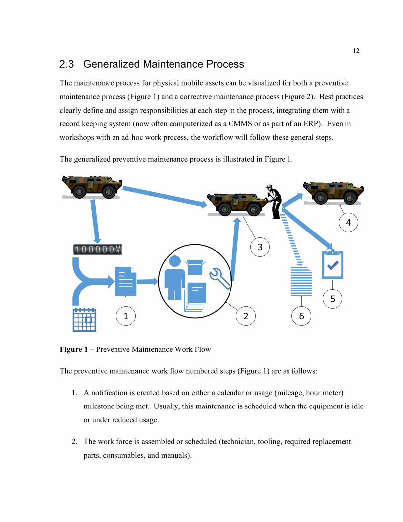
The maintenance process for physical mobile assets can be visualized for both a preventive

maintenance process (Figure 1) and a corrective maintenance process (Figure 2). Best practices

clearly define and assign responsibilities at each step in the process, integrating them with a

record keeping system (now often computerized as a CMMS or as part of an ERP). Even in

workshops with an ad-hoc work process, the workflow will follow these general steps.

The generalized preventive maintenance process is illustrated in Figure 1.

1 2

3

4

6

5

Figure 1 – Preventive Maintenance Work Flow

The preventive maintenance work flow numbered steps (Figure 1) are as follows:

1. A notification is created based on either a calendar or usage (mileage, hour meter)

milestone being met. Usually, this maintenance is scheduled when the equipment is idle

or under reduced usage.

2. The work force is assembled or scheduled (technician, tooling, required replacement

parts, consumables, and manuals).

13

3. The work force and the equipment are brought together, either in the shop or in-situ (the

equipment’s location) based on the local situation.

4. Once the preventive maintenance is complete, the work order is finalized and filed.

5. The equipment is released to operation.

6. If the preventive maintenance has discovered corrective maintenance that cannot be

completed (due to timelines based on local policy), a corrective notification/work order

is created. Depending on the severity of the fault, the equipment can be released to

operation with no restrictions, released to operation with restrictions, or queued into

corrective maintenance.

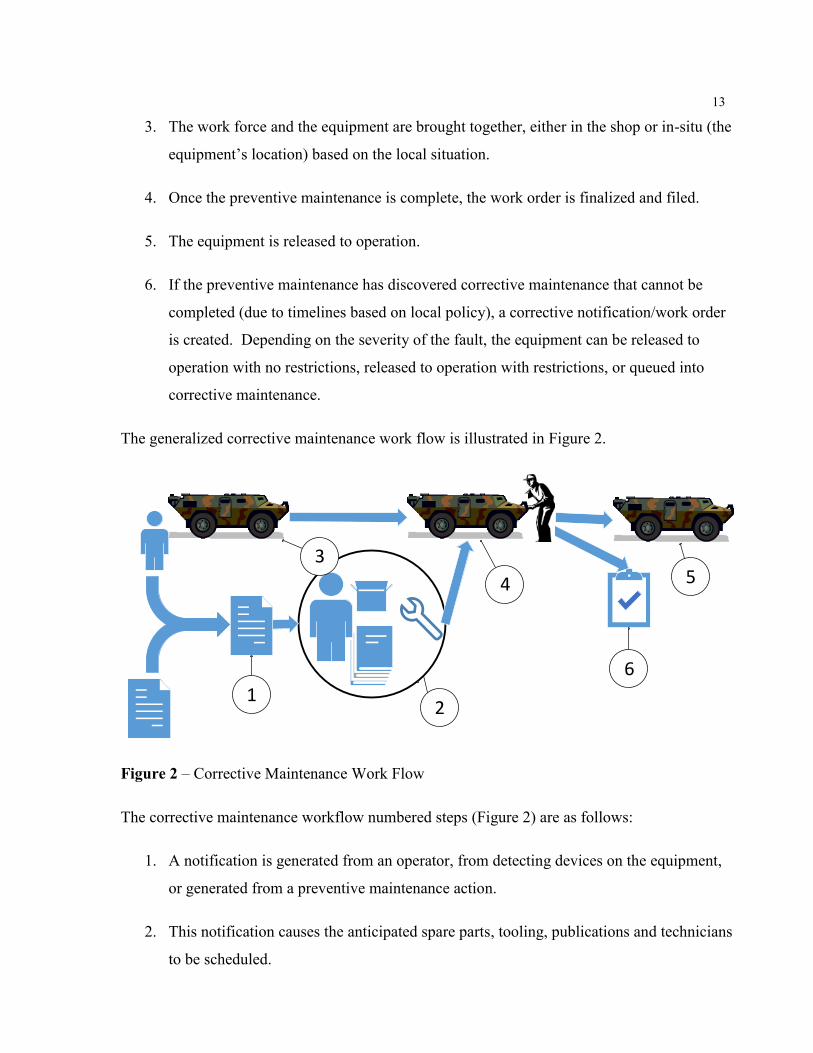
The generalized corrective maintenance work flow is illustrated in Figure 2.

12

3

4 5

6

Figure 2 – Corrective Maintenance Work Flow

The corrective maintenance workflow numbered steps (Figure 2) are as follows:

1. A notification is generated from an operator, from detecting devices on the equipment,

or generated from a preventive maintenance action.

2. This notification causes the anticipated spare parts, tooling, publications and technicians

to be scheduled.

14

3. The equipment is called in for maintenance action.

4. The maintenance action is performed using the assembled resources.

5. Once the maintenance action has finished, the equipment is released to service.

6. The work order is finalized and filed.

Modification processes are similar to corrective processes, with the original notification

generated from some type of engineering analysis. Ideally, the publications and replacement

parts will be assembled into a package and provided to the workshop conducting the work. In

certain circumstances, this package may also include external labour (in the case of a highly

technical or labour intensive modification).

2.4 Data Capture

The data are captured for the ERP system at multiple points in Figure 1 and Figure 2. While in

theory, this means the data can be checked at multiple points, in practice, there may be multiple

sources of error. Further, as there are multiple data entry points, the persons doing the data

entry can become complacent and skip the data entry on those points for which they neither

know the purpose nor receive any benefit for entering. Appendix A and Appendix B detail

where some of the data used in this study are sourced. For an ERP system, the linking of data

between modules (e.g. maintenance to finance) can become quite complex.

2.5 Preventive Maintenance

2.5.1 Definition

Preventive1 maintenance has various and sometimes conflicting definitions. The Canadian

Government’s official lexicon (Termium Plus®) says the following:

1 From the Merriam-Webster dictionary[5]:

Preventative adjective or noun, definition: Preventive.

It further says:

Preventive noun: something that prevents; especially : something used to prevent disease,

15

Maintenance intended to reduce the probability of failure or the degradation of a

functional unit [6] (taken from the Canadian Standards Association Information

Technology Vocabulary).

However, Termium Plus® also calls up a second reference:

NATO’s official definition is “Systematic and/or prescribed maintenance intended to

reduce the probability of failure” [7, p. 2–P–8].

Elsewhere, preventive maintenance is defined as:

Scheduled downtime, usually periodical, in which a well-defined set of tasks, such as

inspection and repair, replacement, cleaning, lubrication, adjustment, and alignment are

performed [8, p. 219].

Preventive maintenance or scheduled maintenance. Equipment is serviced and/or

components replaced at regular fixed intervals [9, p. 139].

Any action performed on equipment at periodic intervals with the aim of preventing

failure in service and retarding deterioration [10, Ch. GL–E–1].

Scheduled maintenance tasks performed before equipment failure to prevent it from

occurring [11, pp. 4–40].

Maintenance performed at predetermined intervals or according to prescribed criteria in

order to reduce the probability of failure or the degradation of the functioning of a

functional unit [12] [13].

The maintenance carried out at predetermined intervals or corresponding to prescribed

criteria and intended to reduce the probability of failure of the performance degradation

of an item [14].

The care and servicing by personnel for the purpose of maintaining equipment and

facilities in satisfactory operating condition by providing for systematic inspection,

detection, and correction of incipient failures either before they occur or before they

develop into major defects [15].

Simple or minor preservation operations and the replacement of small standard parts not

involving complex assembly operations [16].

Preventive adjective: : devoted to or concerned with prevention : precautionary <preventive steps against

soil erosion>: as

a : designed or serving to prevent the occurrence of disease <preventive medical care>

b : undertaken to forestall anticipated hostile action <a preventive coup>

16

2.5.2 Preventive Maintenance Themes

Several common themes are evident across these definitions. The first is a reduction in failures.

The second is periodicity, or a set time or interval in which maintenance is performed.

Therefore, to enact an effective Preventive Maintenance plan, those actions that will lessen the

risk of failure must be determined, and the correct or ideal interval must be selected.

Not included in the definitions is the goal of preventive maintenance. Several possibly

conflicting goals are evident: lowest possible operating costs, least possible downtime, and/or

greatest possible system availability, reliability, and/or availability of a group of systems. The

goal of the preventive maintenance program for the system must be in line with corporate goals

or expectations.

2.5.3 Industry Differences

What may be suitable for one industry may not be the preventive maintenance goal of another.

For example, a mining company may seek the least possible downtime of haul trucks when the

market for ore is high, and it may seek the lowest possible operating costs during normal

operation. If an industry has a high penalty for breakdown costs (i.e. unplanned idle time is very

expensive) it may seek the lowest operating cost tied to the least possible unplanned downtime.

Further, an industry with many standby systems (e.g. parallel safety systems) may seek a certain

percent reliability, such as a parallel pumping system that needs 5 of 7 pumps operating in order

to have an appropriate flow.

2.5.4 Lowest Operating Cost and Least Possible Downtime

Many of the definitions noted above refer to degradation of the unit and allude to downtime. To

understand the need for preventive maintenance, we must understand the effects of degradation,

downtime, and operating costs on the local situation. More specifically, these must be defined

with respect to the operating conditions in that situation or in that corporation.

2.5.4.1 Degradation

Worn items may have degraded performance. For example, dirty filters may restrict flow,

lengthening the production process and affecting the output and value per operating hour.

17

2.5.4.2 Downtime

When equipment is not functioning, there is a cost to the organization. If this downtime is due

to a failure or an unplanned shutdown, an elevated cost may be associated with multiple

components:

Idle staff drawing full wages

Penalties from customers due to missed deadlines

Infrastructure costs for heat/power

Lost opportunity costs (i.e. a smelter shut down when metal prices have peaked).

In contrast, planned shutdowns are often associated with reduced costs:

Work planned during times main production staff are not at facility (i.e. on weekends,

during planned shut-downs)

Work scheduled to meet customer deadlines

Infrastructure costs may be reduced as non-essential parts of the facility can be placed in

a low power state

Work planned for times when market values are favourable.

2.5.4.3 Operating Cost

Simply stated, the cost of operation is affected by many things, and cost may not be the same

over a period of time. Preventive maintenance must take this into consideration.

2.5.5 Refined Preventive Maintenance Statement

While the above definitions are useful, they all lack a “so what” type of statement. An effective

and clear definition of preventive maintenance needs to incorporate a goal statement. In other

words, preventive maintenance is intended to do or to accomplish “what”.

Ebeling provides a clear definition of preventative maintenance: “[It] is scheduled downtime,

usually periodical, in which a well-defined set of tasks, such as inspection and repair,

replacement, cleaning, lubrication, adjustment, and alignment are performed”[8, p. 219].

Adding an accomplishment statement such as “… in order to achieve the lowest possible

operating cost” or “… in order to achieve an X% system reliability” completes the definition

required in government or industry.

18

A clear definition of preventive maintenance is required for all members of an organization to

understand the requirements and goals. An unclear or incomplete definition can result in an ill-

defined preventive maintenance policy.

2.5.6 TLAV Preventive Maintenance Policy Review

Preventive maintenance for the TLAV is divided into various stages performed by different

persons. The first is the operator’s daily pre-use inspection, to be done prior to use. The second

is the operator’s periodic (or weekly) inspection, a more comprehensive inspection. The final is

the semi-annual preventive maintenance inspection and repair performed by the maintenance

technicians. This inspection occurs every six months unless the vehicle has been placed in a

state of long-term preservation.

Semi-annual inspections are typically the responsibility of first line organizations, but may be

performed by the third or fourth line if the equipment is being held as a strategic reserve stock.

The preventive maintenance instructions for the TLAV are contained in the maintenance

manuals as well as the vehicle inspection check list (known as the 1136 form) and the operator’s

instructions. The maintenance manual details the operator’s daily and weekly inspections as

well as the maintenance technician’s semi-annual inspections. The 1136 form is a generic

armoured vehicle inspection checklist guide. Additionally, a 50-point checklist has been

produced as an aide/guide for operators conducting daily inspections.

A detailed chart of these combined documents and an analysis of the inspection program is

included in Appendix E.

Although the maintenance and the process of conducting maintenance on the TLAV and other

fleets appears sound, until the data contained in the DRMIS ERP can be utilized to track the

performance of the TLAV under various conditions, there is no way to improve current

practices.

19

Chapter 3

Data Synthesis

3.1 The Information Pyramid

The collection and use of data can be represented by the Information Pyramid, also known as

the DIKW (Data-Information-Knowledge-Wisdom) Pyramid, as proposed by R.L. Ackoff[17]

(note: earlier versions of this model may also exist). Figure 3 shows the Pyramid.

Figure 3 – DIKW Pyramid

When a CMMS/ERP is being developed, the developers must understand how the data are going

to be used if they are to create methods to properly categorize the data. If the data are going to

be transformed to be used in corporate decision making as knowledge or wisdom, their

20

treatment will differ from that of data held for a short duration and not transferred up the

pyramid.

When data are being collected, the chief issue is how they will be used. Is it appropriate to

collect data for short term use and dispose of them, or must they be stored for future use? If the

latter is the case, many questions arise: for example, how are those data to be structured to allow

retrieval, and what items of data are to be captured?

If not enough data are captured, they may not be useful in the future, as key items may be

missing. But if too many data are captured, their organization and storage can become

problematic. All the data and more may be there, but the relevant data may not be immediately

discernible. Although there are various techniques to parse the data, if this is beyond the

capacity or capability of the organization holding the data, the organization is no better off than

if it held none.

Additionally, capturing more data, in this case maintenance data, requires either more sources

(automated reporting of sensors, mileage, etc.) or more data entry by human operators/

technicians or both. This may become costly in the form of infrastructure cost or the cost of

worker-hours spent entering data. Further, if there is a human involved in the capture or input

of the data, these data can be incorrectly entered, or if the task is long and laborious, it may be

neglected.

3.2 Sources of Data

Multiple data sources and repositories are often available, but organizing them to allow analysis

can be complex. Data sources may take the form of multiple computer record systems, paper

records, or even expert knowledge.

In the TLAV, data were available from: two separate maintenance logs, the original CMMS

(PLANN Expert) and the new ERP system (DRMIS). Data were also available in: Condition

Based Monitoring (CBM) (SOAP records database); a mileage tracking database (Fleet

Management System - FMS); maintenance publications; and a parts cataloguing database.

21

As the TLAV was brought into service before the DRMIS ERP was released for use, the vehicle

maintenance work orders existed in the CMMS but were closed out on the CMMS; the vehicles

transitioned to the ERP as it was rolled out by the Canadian Forces (on a location-by-location

ERP implementation). The transition to the ERP was not simultaneous for all vehicles at all

locations.

Although it did not exist in this case due to the relatively young age of the re-built vehicle

system, it is not uncommon to find paper copies of work orders. For example, a recent study of

replacement wooden electrical poles had this problem. As the poles had a lifetime exceeding 80

years, the full data were captured on both paper and electronic spreadsheets [18].

The database used in this study contains data on a lifetime of CBM. Unfortunately, as the data

were recorded and submitted by local technicians, the component specific identification

numbers were not properly recorded and the data could not be linked to a specific item of

equipment. When CBM data are properly organized they can be used to develop a PHM which

is based on internal (diagnostic) variables.[19] All of the elements of the SOAP analysis (i.e.

ppm of different metals) can be analyzed to determine which of these internal covariates are

reflective of the current state of the component.

Expert advice and tacit knowledge is often an untapped source of data. For the TLAV, such

data came from the project staff and technicians working on the vehicle. Updates to information

not captured in the publications were only available from experts, and this was used in the

characterization of the ERP/CMMS data.

3.3 The TLAV CMMS/ERP Dilemma

In the case of a CMMS or a maintenance module as part of an ERP, the immediate purpose of

the system may not be to capture data to convert them into wisdom, but to notify the appropriate

authorities that a repair or inspection is required and to facilitate the planning required to put the

failed equipment, parts, publications, and technicians (Figure 1 and Figure 2) into the right place

at the right time for repair. This may neglect some of the data required to fully define the failure

to allow the automated output of knowledge or wisdom, as the technicians are more concerned

with completing a repair than with characterizing the type of failure, its cause and effect.

22

This lack of data fitness (missing, improperly captured or structured data) is addressed in a

conference paper as part of a collaboration between the Centre for Maintenance Optimization

and Reliability Engineering (C-MORE) and the Faculty of Engineering, Computing and

Mathematics, University of Western Australia [20]. The paper addresses some of the issues

observed in the analysis of the CMMS and ERP data for the TLAV investigated in this thesis.

This failing in CMMS’ ability to process data was termed the “Black Hole” by Labib[21].

”Black hole” systems are “greedy for data input [but] seldom provide any output in terms of

decision support” [21, p. 192]. Labib adds:

Companies consume a significant amount of management and supervisory time

compiling, interpreting and analysing the data captured within the CMMS.

Companies then encounter difficulties analysing equipment performance trends

and their causes as a result of inconsistency in the form of the data captured and

the historical nature of certain elements of it. In short, companies tend to spend a

vast amount of capital in acquisition of off-the-shelf systems for data collection

and their added value to the business is questionable.[21, p. 192]

Unfortunately, this appears to be the problem with the data used in this study. The ability of the

CMMS to process day-to-day maintenance transactions is at odds with the ability to provide

integrated, seamless decision analysis.

The data accumulated in the CMMS and ERP used for this thesis seem to be concentrated or

focused on “getting the job done”. The data appear to be those required to get the parts ordered

and the vehicle into the shop to do the repair, and then close the work order to go on to the next

job. This concentration on conducting the repair and collecting data for the purpose of

conducting the immediate repair is evident and is a detriment to subsequent study and analysis.

Several key deficiencies are the result.

3.3.1 Lack of Failure Mode or Failure Cause

Failure modes are “the manner by which a failure is observed. Generally describes the way the

failure occurs and its impact on equipment operation”[22, Para. 3.1.14]. Examples of potential

failure modes include:

23

Corrosion

Hydrogen embrittlement

Electrical short

Fatigue

Deformation

Cracking [23]

A failure cause is “the physical or chemical process, design defects, quality defects, part

misapplication, or other process which are the basic reason for failure or which initiate the

physical process by which deterioration proceeds to failure” [22, Para. 3.1.12]. Examples of

potential failure causes include:

Improper torque applied

Improper operating conditions

Contamination

Improper alignment

Excessive loading

Excessive voltage[23]

A failure effect is “the consequence(s) a failure mode has on the operation, function, or status of

an item. Failure effects are classified as local effect, next higher level, and end effect”[22, Para.

3.1.13]. Examples of failure effects include:

Injury to the user

Inoperability of the product or process

Improper appearance of the product or process

Odours

Degraded performance

Noise[23]

The work orders (WOs) used by the fleet studied here did not capture these failure data, thus

limiting the possibility of further research and refinement of preventive maintenance actions.

The WOs did capture the occurrence of failure, but did not indicate why or how a failure

occurred.

24

Failure mode data could be captured in a field within the ERP data entry screen. The usefulness

of capturing these data must be weighed against the added processing time for the work order.

Further, as can be seen in the existing databases, if these fields are left for free-form data entry,

the number of possible responses (including abbreviations and misspelling) grows with

continued usage of the ERP. A further option is the use of a drop-down style list; however, this

can lead to data entry operators either choosing the first item on the list or selecting “unknown”

in order to proceed to the next step of the ERP process. This operator devaluing of the data can

be reduced by training and supervision, as well as ensuring the data entered can be manipulated

and improved and returned to the operator as either information or knowledge (a higher level on

the DIKW pyramid).

3.3.2 Lack of Clear Dates

The WOs all contained dates of return to service and hours in maintenance, but these dates do

not indicate when the item went into maintenance in all cases.

Some failures are hidden, and only express themselves when that system is selected for use;

these failures have a range of dates over which they may have failed. Further to this, poor

operator accountability means failures are not reported when they are noticed, as the operator

may want to use the system and may fear that reporting a failure could take the system out of

operation for maintenance. Operators may choose to continue using a failed/failing system,

further damaging other items in that vehicle, resulting in more extensive repair costs. For

example, an operator may identify a leaking turbo oil line but decide not to report it. This could

cause the turbocharger to become oil starved and fail, possibly damaging the engine. A $20

repair could quickly become a $20 000 repair.

3.3.3 Freeform Text

Data entered into several fields (WO Description, PM order_Description and Opr_short_ text)

were free form, user entry data. The information was inconsistent, prone to spelling errors, and

written in both French and English. The fields contained everything from detailed text

descriptions to text that simply said “repairs” (with no indication of what was repaired).

25

Further, the descriptions for some work orders differed from the work actually done. In several

cases, the description referred to repairs to one system on the vehicle, but the parts used

included components that could be installed on other systems/locations on the vehicle.

Furthermore, the descriptions could not capture opportunistic repairs done when the vehicle was

in the repair shop. Once the work order was created and described, any additional repairs

needed or found by the technician would not be included in the description.

3.3.4 Incomplete Component Identification

Key components are identified with a unique serial number, often marked on re-buildable

components such as engines and transmissions. If the location of each of these components is

known throughout their lifetime, their usage and status can be tracked. Further, bad actors can

be eliminated (i.e. those engines that even after rebuilding have shortened service lives, due to

undetected damage or re-manufacturing that has taken such items as cylinder walls outside of

specifications).

Unfortunately, the tracking of serial numbers was not implemented in the data provided, a key

reason why the SOAP database had become corrupt.

As well, several components on the vehicle lacked locational identification. The vehicle

contains many components with the same part number which can be used in multiple locations;

for example, the final drive can be used on either the right or left side, but the work order, in

many cases, did not denote which side was changed. The problem of parts used in multiple

locations extended to parts lacking serial numbers, such as road wheels, suspension arms,

shocks etc. It becomes difficult to tell if the same shock is being changed each time or if one of

the other shocks on the vehicle has failed and is being replaced.

3.3.5 Poor recording of usage data

This particular vehicle is equipped with an odometer, as well as an engine hour meter. The

engine hour meter information was not captured in the data. The vehicle mileage was captured,

but as this was a manual entry, the data were subject to corruption. Further, if an odometer was

repaired, or reset, subsequent mileage recordings did not necessarily capture this adjustment.

26

3.4 Remedies

Several solutions were implemented while cleaning the database for inclusion in the study. The

lack of failure mode data could not be overcome and was not the focus of this thesis. The

inclusion of failure mode data, if they existed, could help define “wisdom,” thus allowing the

analysis to define problem areas, leading to possible changes in system engineering. As it

stands, any engineering change would require extensive study and testing. The current data can

provide information on a troubled sub-system but lack the wisdom required to find a solution.

The lack of clear dates and mileages introduces a range of error for each of the failures, but in

light of possible security implications or perceived security implications, this error was allowed

to stand. If these data are to be cleaned for internal DND use, further operator training and

enforcement are required.

3.4.1 Component Identification

Component Identification was done manually, by comparing the NATO Stock Numbers (NSNs)

of the parts used in the repair with the parts manual that included descriptions and an exploded

parts diagram showing where the NSN was used on the vehicle. In most cases, this was enough

information to properly identify the part. For example, if the NSN was called a gasket, the

exploded parts view would show exactly which gasket and where it was used on the vehicle (i.e.

a gasket -> valve cover -> used on the engine). This identification allowed each line item in

each work order to be characterized using a coding system.

3.4.2 Work Order Coding

Each work order was coded, allowing all work orders to be easily grouped along various search

strings. As there may have been several repairs conducted or actions taken on each work order,

there may be several codings per work order. For example, if a work order was opened to

perform a repair on an engine, there could be a SOAP test, along with repair parts called up for a

sub-component turbocharger and a sub-component alternator. In coding the work order, all

three would be coded, as they served different purposes. Further, as previously mentioned, if

opportunistic maintenance occurred, e.g. repairs to the track, this was coded against the work

order where the parts were used.

27

Work Order Coding used four fields to describe the work to reach the level of fidelity required

for this study: Maintenance Type, Component, Sub-Component, and Action. This coding

allowed each work order line to be characterized with a seven digit code.

3.4.2.1 Maintenance Type – Maint_Type

The type of maintenance taking place was determined based on the description of the work and

the parts used, if any, to conduct a repair. These were categorized as shown in Table 1.

Table 1 – Maintenance Type Coding

Maint_

Type

Description Usage

C Corrective Repairs corrective in nature, repairs of parts, replacements of parts.

Most WOs using parts fell under Maint_Type Corrective. Database

records described as inspections but using repair parts were

categorized as corrective, as this relates to the failure of a

component.

I Inspection Inspection of equipment to determine its status. WOs described as

inspections in the comments field may have several database

records: one line without any repair parts called up would be coded

as Inspection, and the remaining lines calling up repair parts coded

as Corrective (that is, those faults found upon inspection).

M Modification Modifications are changes to the baseline system as directed by a

higher maintenance authority. Modifications were noted in the WO

description, and in the use of specific modification kits on several

modifications. Modifications affect the system by potentially

removing serviceable components to replace them with newer or

improved ones. Track modification is an example of this: existing

serviceable steel link tracks are replaced with a rubber continuous

band track to gain an operational and tactical advantage.

P Preventive Repair actions inherently preventive in nature include changing oil,

replacing engine belts etc.

X Exclude WOs noted as duplicate, cancelled or with sub components (nuts and

bolts) used on multiple components could not be uniquely identified

and were excluded.

3.4.2.2 Component – Comp

The coding “Comp” is a description of the major system affected by the Maintenance Type. On

a single work order, multiple components may have been affected, and all were captured with

the coding shown in Table 2.

28

Table 2 – Component Type Coding

Comp Component Description

CC Crew

Compartment

Components affecting the crew area (seats, stowage etc.)

CO Controls Operator controls

CS Communication

Systems

Radios and associated hardware, including antennae and

mounts

DL Driveline Engine driveline (shafts, universal joints)

EL Electrical Major vehicle electrical, not directly associated with another

component

EN Engine Vehicle engine and associated components

FD Final Drive Final drives transfer power from the drive shafts to the drive

sprocket that moves the track

FU Fuel Tanks, lines and pumps

HU Hull Vehicle hull, including bins, mounts and hatches

HY Hydraulics Lines, pumps, filters, cylinders

OT Optics Weapons sights and vision devices for the driver

PP Power Pack Engine and transmission when combined as a single

component

SU Suspension Shocks, support arms, idler arms

TK Track Originally a steel track, later the continuous rubber band track

TR Transmission Vehicle transmission

VE Vehicle Entire vehicle, typically used when denoting the semi-annual

inspection of the vehicle

WS Weapon System Any component associated with the weapon system, including

the turret or weapon station

XX Exclude WOs noted as duplicate, cancelled or with sub-components

(nuts and bolts) used on multiple components that could not

be uniquely identified and, thus, were excluded

3.4.2.3 Sub-Component – Sub_Comp

“Sub-Component” is a descriptor to further define the parts used to repair a component. Sub-

components do not uniquely identify an item; for example, a bolt could be used on different

components. In order to define an item, each data entry must be read as follows: Component

first, then Sub-Component (i.e. FUFI = Fuel Filter, HYFI = Hydraulics Filter). The Sub-

Component codes are listed in Table 3.

29

Table 3 – Sub-Component Type Coding

Sub Sub-Component Usage (Component Higher Assembly)

00 None Not Required, or entire competent changed; thus, no sub-

components used

AF Air Filter Engine

AL Alternator Engine

AO Add On Armour Hull

BE Belt Engine, Crew Compartment (Seat Belts)

BI Bin Crew Compartment, Hull, Weapon System

BO Bolt Multiple

BR Brakes Transmission, Control, Crew Compartment

BT Battery Electrical

CA Cable Communication System, Electrical, Weapon System

CO Cover Multiple

DS Drive Shaft Drive Line

EL Electrical Engine, Weapon System

EX Exhaust Engine, Crew Compartment

FA Fan Engine, Crew Compartment

FI Filter Engine, Hydraulic, Fuel, Transmission

FL Fuel Lines Fuel, Engine

FP Fuel Pump Fuel, Engine (high pressure pump)

FR Fire Suppression Hull, Electrical

GU Gauge Control, Electrical

HA Hatch Hull

HE Heater Engine, Crew Compartment

HR Horn Control, Hull

IA Idler Arm Suspension

IW Idler Wheel Suspension

LF LEFT Track, Final Drive

LI Light Hull, Crew Compartment, Weapon System, Electrical

MI Mirror Hull

MO Mount Communication System, Engine, Hull

OP Oil System Engine, Transmission

PA Pad Track

PL Plug Hull, Engine

30

Sub Sub-Component Usage (Component Higher Assembly)

PT Plate Hull

PU Pump Engine, Hydraulic

RA Radiator Engine

RE Receptacle Electrical, Weapon System

RR Ramp Rear Hull

RT RIGHT Track, Final Drive

RW Road Wheel Suspension

SA Support Arms Suspension

SC Super-Charger Engine

SE Seat Crew Compartment

SF Shaft Multiple

SH Shock absorber Suspension

SI Sighting Systems Weapon systems

SK Sprocket Drive line, Engine

SN Sensor Multiple

SP Speedometer Control, Transmission

SR Steering Control, Crew Compartment

ST Starter Electrical, Engine

SW Switch Multiple

TA Tank/Reservoir Fuel, Hydraulic

TB Torsion Bar Suspension

TC Turbo-Charger Engine

TE Tensioner Engine, Suspension

TU Tubes / Hoses Multiple

UK Unknown Sub-components (nuts and bolts) used on multiple components

that could not be uniquely identified

VT Valve Train Engine

WI Windshield Hull

XX Exclude WOs noted as duplicate, cancelled or unable to be characterized

were excluded

3.4.2.4 Action – Maint_Action

“Action” describes what the technician did on a particular data entry. These are listed in Table 4.

31

Table 4 – Maintenance Action Coding

Action Description Usage

00 Inspection Inspection of an item without repair

AD Adjust Physical adjustment, no parts used

FL Change fluids Oil or other fluid change

IN Install Install a new item, no removal of an old item (e.g. install Add-

on-Armour)

LU Lube Lubrication

PR Preservation Placing an item in long term storage, cleaning an item, or

removing moisture

RC Recovery Extraction of a stuck vehicle

RE Replacement Removal of a component and installation of a new component

RM Remove Removal of a component without re-installation (e.g. removal of

Add-on-Armour)

RP Repair Fixing an item without replacement (e.g.. tightening loose

mounting bolts)

SC Sub-Component

Replacement

Replacement of a sub-component or sub-sub-compoenent that is

not traceable.

SO SOAP Test Spectrometric Oil Analysis Program fluid sampling

UK Unknown Insufficient details to characterize the action

VM Vehicle

Movement

Inspections completed, sending or receiving a vehicle from

another location

XX Exclude WOs noted as duplicate, cancelled or unable to be characterized

were excluded

3.4.2.5 Coding Steps

The work order coding was a manual multiple step process:

1. Data lines with no parts usage and a description referencing inspection were coded

(typically with an I code).

2. Data lines with no parts usage were analyzed to determine the proper coding.

3. Data lines with a description of a modification were coded (typically with an M code).

32

4. Parts used on a data line were analyzed; each part number was set against an exploded

parts view to confirm where it was used on the vehicle and whether it was coded

appropriately.

Because the parts had to be looked up and visually confirmed against the exploded parts

diagram, it was not possible to fully automate the coding process. Considerable programming

would be required to have an automated system look up a part number and interpret an exploded

parts view. The lookup process might be simplified if the parts database were fully

characterized into parts dependencies.

Information that was not available or could not be characterized (blank lines, inconsistent data)

was coded with an X or XX. If it could be determined that a corrective action happened in the

crew compartment, but no other information was available, it was coded C-CC-XX-XX.

An example of the CMMS and ERP data sets available for the study and the subsequent coding

can be found in the appendices (Appendix D– CMMS Database Sample and Appendix E– ERP

Database Sample)

3.4.2.6 Data Codes

A vehicle inspection is coded as I-VE-00-00, while the replacement of a turbo-charger gasket is

C-EN-TC-SC. This allows quick searching of number of repairs to specific systems, or to focus

analysis on a particular type of maintenance, system or sub-system.

Although this detail is sufficient for this thesis, to fully define the location of every sub-

component down to the location of every nut and bolt would require several more levels of

definition and would need to be captured during the initial collection of the data. It is possible

to have coding capturing the location of the front left washer that secures the driver’s seat to the

floor, but this need to be weighed against the time taken to enter the data and the possible

introduction of errors if there is to be an advantage in moving the DIWK pyramid.

33

3.4.3 Vehicle Usage Calculation

Although it is a data field in the CMMS and ERP, usage data (accumulated kilometres) was not

consistently or properly captured for the fleet. Several error types were discovered during data

analysis:

1. Data were not entered – Null entry field

2. Re-set odometer settings were not captured – Decrease in odometer readings

3. Use of the same odometer readings over several maintenance periods – Data used from

the previous work order vs being read from the vehicle

4. Erroneous entries – Vehicle license plate or vehicle type identifier entered in field

5. Quick/rough data entry – Rounded values being entered, i.e., 900 vs 898 or 888 vs a

precise amount

Augmenting the usage data captured in the CMMS/ERP were separate odometer readings

captured in a transportation log (FMS). This system is, in theory, updated monthly by entering

the km accumulated in that month. Thus, by knowing the most current reading and subtracting

the monthly accumulated distance readings, the odometer reading in a particular month can be

determined. Unfortunately, typically for each vehicle, a large error accumulated as the

odometer reading went back to the beginning of the vehicle’s life. This accumulated error could

stem from several additional errors:

1. Double entries

2. Large corrections – Data entered, then accumulated and re-entered showing a large

single month increase

3. Not accounting for odometer resets

4. Data transcription errors

5. Inability to correct previous erroneous entries

34

Because these vehicles did not receive homogenous usage over time or across platforms, the use

of accumulated calendar time would not provide an adequate description of the state of the

vehicle. Therefore, usage data are required for even the most basic analysis of the status of the

system. To achieve an acceptable level of clarity, a manual analysis of all available usage data

was compiled as follows:

1. The vehicle was assumed to have 0 km at the beginning of life.

2. The FMS data over the life of the vehicle were plotted on a monthly basis.

3. This was compared to the sparse usage data from the CMMS and ERP.

4. For each vehicle, the data were adjusted up or down to pass through the 0 km origin and

the majority of the CMMS/ERP data points. The increase in month by month usage

came from FMS. Thus, erroneous data quickly became visible and could be addressed

or deleted.

These corrected data could be used to determine the km reading in the month the equipment

failed or an event (inspection, modification) took place. This was confirmed in the EXAKT

program by looking at the life history plots for the vehicles (see Chapter 5, Figure 4).

3.5 DIKW Conclusions

As seen in the actions taken to “clean” or categorize the data collected in the CMMS/ERP, it is

possible to take data “sitting” at the bottom of the pyramid and move them up the pyramid to

better data/information, but this process is laborious and requires considerable manual input

from an individual who is well-versed in both the equipment being analysed and the culture of

the organization entering the original data.

The easiest solution to the retroactive data categorization problem is to develop and enforce a

coding system at the time of work order creation. Through the use of smart drop-down tables,

technicians can be presented with a tailored series of options to characterize the repair they are

doing. These smart drop-down tables would aim not to overwhelm the technician with options,

allowing for subsequent accurate and precise analysis of the data.

35

Chapter 4

Operating Condition Effects

4.1 Vehicle Usage

Vehicle usage in a military context can vary greatly from other industries. The military vehicles

are often moved between locations for varying durations to perform training or on missions. A

vehicle may experience hot and dusty conditions one year before being moved to a different

mission in a cold/wet environment under a different mission profile (task profile).

Many other managers of large fleets experience vehicle usage patterns that are more suitable to

a stable homogeneous analysis. For example, mining haul trucks tend to operate in a particular

mine for their entire lifetime under nearly continual usage. Transit buses in a city operate under

fairly consistent conditions with minor cyclical variations for the seasons.

The use of covariates was investigated extensively by Ghodrati when applied to mining

vehicles; however, these conditions were site specific as the subject vehicles passed their entire

life in the same geographic location, performing the same task [24-27]. Covariates were used

by Barabadi when investigating seasonal changes to equipment (oil and gas platforms and

electrical meters) in a fixed location [28], [29]. Furuly (with Barabadi) studied operating

environments (winter to summer) in the Svea coal mine in Norway[30]. However, these studies

did not have the opportunity to investigate equipment moved between various environments.

Military vehicles are ideal for this sort of study; they are exposed to a wide range of operating

conditions and usage intensities. A vehicle may sit for long durations waiting to be sent on a

mission; while on the mission, it may see extremely high usage. In addition, military vehicles,

especially in Canada, can experience a wide range of environmental conditions, from cold to

extreme heat while on a mission. However, little work in the analysis of moving military

vehicles between environmental conditions is available. Wong in her Master’s Thesis looked at

SOAP covariates for the British Warrior armoured vehicle, and proposed in future work to look

at temperature conditions and their effect in a single training location[31].

36

In light of this, a covariate model was needed to address the possible differing conditions faced

by the vehicle and to determine if the generic model could be improved.

4.2 Environmental Conditions

Four general environmental conditions define the conditions faced by this fleet (TLAV FOV):

Cold, Hot, Wet, and Dusty.

Other environmental conditions could be faced by the vehicle fleets, including extreme cold, salt

spray etc.; however, during the period of study, these vehicles did not encounter such

conditions.

In order to study the conditions faced by the vehicles, a system of quantifying the trending

environmental condition in each geographic area had to be developed. The environmental data

from each of the relevant locations over 2001-2013 were acquired (primarily Environment

Canada data). These data showed monthly averages, maximums and minimums; however,

using this type of data quickly became cumbersome.

The use of established baselines was selected as a suitable approximation. NATO’s Allied

Environmental Conditions and Test Publication, AECTP-230 [32], maps out the environmental

trends experienced in every geographic location globally. AECTP-230 was developed to allow

test and project engineers to prepare test specifications for specific climatic effects. AECTP-

230 uses 11 categories found at the land surfaces of the world, and a further three to describe sea

conditions. Test conditions are unusually specified by selecting a condition from the high

temperature category (A1, A2, or A3) and the low temperature category (C0, C1,C2, C3, or C4),

as well as the high humidity category (B1, B2, or B3 if required), based on geographic location

where the equipment will be employed.

As AECTP-230 characterizes the world’s surface temperature conditions, it was chosen as the

basis for the covariate development. The AECPT-230 categories are summarized in Table 5

[32, p. 141].

37

Table 5 – AECPT-230 Summarized Temperature and Humidity Cycles World Wide

Category Meteorological

Temperature (oC) Relative Humidity (%)

Hot (Arid conditions)

A1 32 to 49 8 to 3

A2 30 to 44 44 to 14

A3 28 to 39 78 to 43

Humid

B1 (Jungle)

7 days at 24 100

358 days at 23 to 32 88 to 66

B2 (Savanah) 26 to 35 100 to 74

B3 (Persian Gulf) 31 to 41 88 to 59

Cold

C0 -6 to -19

Tending

to

saturation

C1 -21 to -32

C2 -37 to -46

C3 -51

C4 -57

Maritime

M1 29 to 48 67 to 21

M2 25.5 to 35 100 to 53

M3 -23 to -34 Tending to saturation

4.2.1 Cold

Each location for which the vehicle was used was assigned a score in accordance with the

AECTP-230 cold map (Plate 2). Scores were assigned in a binary fashion. If it met the

condition C0 (mild cold), C1 (intermediate cold), C2 (Cold), C3 (Severe Cold), or C4 (Extreme

Cold), it was assigned a score of 1; otherwise, it was scored 0.

38

Plate 2 – Climatic Categories Map: Cold [32]

The vehicles in this study experienced conditions of C0, C1, and C2, based on geographic

location (confirmed by comparing the Environment Canada norms in each target location to

Table 5). As these vehicles did not operate in C3, or C4, no scoring was performed, and these

values were discarded. If there was a data set with C3 and C4 exposure, based on future

operating conditions, those data would have to be captured and analyzed later.

4.2.2 Hot

Each location for which the vehicle was used was also assigned a score in accordance with the

AECTP-230 Hot map (Plate 3). Scores were given a binary assignment of 1 or 0 if they were in

those conditions (A1 (Extreme Hot Dry), A2 (Hot Dry), A3 (Intermediate)).

39

Plate 3 – Climatic Categories Map: Hot [32]

The vehicles in this study experienced conditions of A3 and A2/A1, based on geographic

location (confirmed by comparing the Environment Canada norms in each target location to

Table 5). One geographic location on deployed operations was on a boundary between the A2

and A1 conditions. As there were no comparison points, and the vehicles in Canada were all at

the A3 condition, to simplify computations, the scoring was modified to either Hot or Not Hot,

scoring a 1 or 0 respectively. If in the future, these vehicles are employed in a geographic

location that can define the difference between A1 and A2, further study will be required.

40

4.2.3 Hot–Humid

The final map used in AECTP-230 defines hot and humid areas (e.g. rainforests and jungles)

(Plate 4). As these vehicles did not operate in any of these conditions, it was not possible to

define the effect on failure, and Hot-Humid was not included as a covariate.

Plate 4 – Climatic Categories Map: Hot–Humid [32]

4.3 Geographic Conditions

Certain conditions create additional strain on vehicles. In this case, bogging was a key

condition that required modeling. Bogging refers to conditions that could cause a vehicle to

become stuck, including wet/muddy ground, soft sandy soil and steep inclines. One location in

Canada met those conditions, as did the deployed location, and they were assigned a score of 1;

otherwise, they were scored 0.

41

4.4 Operating Conditions

Operating conditions influence the serviceability of the vehicles and were defined by three

categories: Operator Experience, Idling Time, and Add-on-Armour.

4.4.1 Operator Experience

These vehicles are used on military operations, on training for missions, on general training and

as training aides for new operators. Because of this, the operator experience level can vary

greatly, placing additional strain on the vehicle. An experienced operator knows how the

vehicle is supposed to perform and can spot small problems before they become damaging.

Locations with experienced operators were scored 1; otherwise, they were scored 0.

4.4.2 Idling Time

Certain locations use the vehicles as training aides, and the vehicles see a high degree of usage,

but low accumulated km. As the engine hour meter readings were not captured, the Idling Time

covariate was created to capture this effect; these locations were scored 1; otherwise, they were

scored 0.

4.4.3 Add-on-Armour

On operations, the vehicles are fitted with an additional armour package. This provides added

protection to the vehicle and crew, but increases the vehicle weight, placing an added strain on

the drive train and suspension. Vehicles with AoA installed were scored 1; otherwise, they were

scored 0.

4.5 Additional Future Conditions

Several other conditions were examined, but there was no way to distinguish them from the

conditions chosen as covariates.

4.5.1 Wet or Dusty

This designation was to be used for locations receiving little moisture. Equipment used in

Canada was assigned a score of 0, while deployed equipment was scored 1. However, this

scoring was identical to the scoring for whether a vehicle had AOA installed, and it was not

42

possible to characterize how dusty a condition may have been at a particular time for the

vehicle.

4.5.2 Extreme Cold

As these conditions were not experienced, they could not be included.

4.5.3 Stagnation

How long a vehicle sits without use likely affects the serviceability of the vehicle platform, as

the system experiences a certain continual degradation due to exposure to the elements. This

exposure leads to corrosion of metals and degradation of rubber gaskets and seals, which can

eventually lead to failure. Unfortunately, from the data available, it was not possible to

characterize stagnation as a covariate based on geographic location.

4.5.4 Rocks/Unprepared Surfaces

Sharp rocks can flatten the tires of wheeled vehicles and damage the suspension and track

components of tracked vehicles; however, in this case there was neither sufficient definition of

rocky areas nor significant differences from other covariates.

4.5.5 Storage

Improperly stored spare parts face various degrees of degradation depending on the types and

harshness of the conditions to which they are exposed [33]. Vehicles left parked and exposed to

the environment also face these deterioration effects. In the initial design, various scores were

to be given based on storage/parking conditions: 0=outside un-covered, 1=outside covered with

a tarp, 2=under a shed/roof, 3=inside a building, 4=in a climate controlled (humidity and

temperature) space. Although the geographic location where the vehicles were stored could be

determined, however, this gave no indication of the specific storage conditions.

4.5.6 Mountainous Terrain

Mountainous terrain causes additional strain on the engine and braking system and can

potentially lead to failure. Unfortunately, there was insufficient mountainous terrain in the

locations where the vehicle was used to be able to include this in the study.

43

4.5.7 Maritime Environment

As exposure to salt spray causes corrosion, an analysis of this condition would be beneficial, but

during the data period, these vehicles were not used in a coastal zone.

4.5.8 General Condition Covariate Summary

Table 6 summarizes the list of environmental/conditions covariates, their coding, and the

scoring mechanism.

Table 6 – Covariate Selection Chart

Condition

Group

Code Condition

Title

Score

Cold

C0 mild cold Score 1 condition; other conditions

score 0 C1 intermediate cold

C2 cold

C3 severe cold

C4 extreme cold

Hot

A1 extreme hot-dry Score 1 condition; other conditions

score 0 A2 hot dry

A3 intermediate

Humid

B1 wet warm Score 1 condition; other conditions

score 0 B2 wet hot

B3 humid hot costal desert

Operator

opexp experienced operator 1 with experience, otherwise 0

Idling

idle equipment idling without

accumulating distance data (if no

hour meter in use)

1 for locations with higher instance

of idling, otherwise 0

Bogging

bog mud, sand or deep snow bogging conditions score 1,

otherwise 0

Armour

AoA add on armour installed 1 for installed armour, otherwise 0

Dust

dust dusty operating conditions 1 for dusty locations, otherwise 0

Stagnation

stag vehicles that tend to sit for

extended periods between usage

1 for locations with equipment

parked/stationary for extended

44

Condition

Group

Code Condition

Title

Score

(if not clearly indicated in the

actual usage data)

periods between usage

Surface

SF0 paved Score 1 the most prominent

operating condition; other

conditions score 0 SF1 gravel

SF2 sharp rocks

Storage

S0 outside un-covered Score 1 condition; other conditions

score 0 S1 outside with tarp

S2 under a roof

S3 inside a building

S4 inside a climate controlled space

Mountain

Mt0 0-500m Score 1 the most prominent


conditions score 0 Mt1 501-1000m

Mt2 1001-1500m

Mt3 1501-2000m

Mt4 2001 and over

Maritime

M1 hot maritime (salt exposure) Score 1 the most prominent


conditions score 0 M2 warm maritime (salt exposure)

M3 cold maritime (salt exposure)

4.6 Condition Covariates

Based on the scoring discussed above, the following initial covariate chart was developed (Table

7). Each of the locations A, B, C, D, E, F corresponds to a location or several locations (if those

locations had the same total scores) where the vehicles were in service. (Place names are

intentionally suppressed.)

45

Table 7 – Environmental Effects

Location Cold 0 Cold 1 Hot Dust Bog

Operator

Experience Idling AoA

c0 c1 hs dust bog opexp idle aoa

A 0 1 0 0 0 1 0 0

B 0 0 0 0 0 1 0 0

C 0 1 0 0 1 0 0 0

D 0 1 0 0 0 1 1 0

E 0 1 0 0 0 1 0 0

F 1 0 1 1 1 1 0 1

Given the locations where this vehicle system was used over its lifetime, Cold 0, Hot, AoA and

Dust have direct dependency and are redundant. As no further details could be determined with

the data set used in this study, they were combined into a single covariate (AoA) representing all

redundant conditions.

4.7 SOAP Analysis

Although SOAP data are often the basis for the covariates for a proportional hazards model

analysis [31], the SOAP data for the TLAV–M113 data set were corrupt and unrecoverable.

Therefore, the integration of SOAP covariates was not pursued.

46

Chapter 5

Proportional Hazards Model Development

The proportional hazards model (developed by Cox[34]; see further work by Banjevic[19])

provides a mechanism to model covariates which may have an influence on the hazard function.

5.1 EXAKT

The developed covariates were run through the condition based maintenance optimization

software called EXAKT (version 4.2).

EXAKT takes processed signals, correlates them with past failure and potential

failure events. Using modeling, it subsequently provides failure risk and residual

life estimates tuned to the economic considerations and the availability

requirements for that asset in its current operating context.[35, p. 125]

The use of EXAKT to calculate geographic influences is not part of the intended design;

however, when covariates are carefully selected, EXAKT meets this extended purpose.

5.2 Data Input

Normally, EXAKT takes readings at each inspection time as inputs for the covariates. These

readings usually take the form of observations from a CBM program (e.g. parts per million

(ppm) of iron (Fe) or copper (Cu) in the oil samples or vibration readings at each inspection

point). For example, a prominent oil analysis laboratory offers 3 levels of SOAP, with the first

level returning readings on 30 contamination, wear and oil condition items, and the highest level

returning over 57 readings[36], [37]. EXAKT solves the proportional hazards model for the

system based on all CBM observations; then, through a process of elimination, the solution is

reduced to those covariates that are significant to the model (as described by Wong [31], [38]).

For this thesis, the environmental covariates were entered as inspection readings based on the

geographic location where the vehicle was located when the inspection was performed (location

where the vehicle was held). Further, for each repair point or equipment suspension point, a

dummy inspection was created based on the vehicle location at the point of repair. This method

47

allowed the establishment of the vehicle’s life history, showing when it entered into service,

each inspection point and any component replacements.

EXAKT requires the data from the ERP/CMMS to be structured into two main spreadsheets that

it uses for its calculations. The first is the “Events” sheet (EXAKT M113 transmission Events

table excerpt at Appendix D) and the second is the “Inspection” sheet (EXAKT M113

transmission Inspection table excerpt at Appendix G).

EXAKT needs to know when the equipment went into service (“B” – Beginning) as well as each

inspection time (“I” – Inspection) and the results of the inspection (covariate

values/measurements). Each failure (“EF” – Equipment Failure) and removal before failure

(“ES” – Equipment Suspension) must be entered with the date and accumulated working age (in

this case kilometres accumulated on the odometer). Additionally, after each EF and ES

occurrence, the replacement component starts its life and thus has a Beginning, in this case

noted as BEF and BES respectively. To allow EXAKT to know where the vehicle was at all

points in time, dummy inspections were created after the initial beginning when the vehicle

went into service “D”, as well as EF and ES occurrences (DEF and DES respectively). These

dummy inspections were treated the same as any other inspection; in the case of these

covariates, it ensured the covariates were applied continually over the life of the vehicle despite

some vehicles changing operating locations during their history.

The final step to ensure the EXAKT data input was appropriately structured was the addition of

a time element to each of the date entries. As multiple events (I, EF, BEF, DEF) could happen

on the same day, the order of the events required a higher level of fidelity; this was

accomplished by giving a time to each event which was then applied to each day that particular

event occurred. This ordering forced a precedence hierarchy on all possible event combinations

(Table 8).

48

Table 8 – Event Precedence

Order

Event /

Inspection Name

Time

(24 hour clock)

1 B Beginning 12:00

2 D Dummy Inspection to initially place vehicle 12:01

3 I Inspection 13:00

4 DEF Dummy Inspection to place vehicle prior to EF 15:00

5 EF Equipment Failure 15:30

6 BEF Beginning after EF 15:45

7 DES Dummy Inspection to place vehicle prior to EF 16:00

8 ES Equipment Suspension 16:30

9 BES Beginning after ES 16:45

The resulting data could then be represented graphically for transmission replacements, as

shown in Figure 4, for each of the vehicles.

Figure 4 – Example EXAKT Equipment Component Life History

49

5.3 EXAKT Simple Weibull Model

Using the life history of the equipment and of both the Equipment Failures (EF) and Equipment

Suspensions (ES), EXAKT calculates the probability density function for the Weibull [35] as

follows:

( )

(

)

( )

( )

Equation 1

where:

β = Shape parameter,

η = Scale parameter (characteristic life),

γ = Location parameter.

It also calculates the hazard rate h(t) [35]:

( ) ( )

(

)

( ) ( )

Equation 2

This can be expressed as the cumulative distribution function F(t) as follows [35]:

( ) ( )

Equation 3

Further, the Reliability Function R(t) can be derived from a known hazard rate [8]:

( ) ∫ ( )

Equation 4

In addition, EXAKT calculates the mean life µ[35, p. 241][39] using the following function:

50

(

)

Equation 5

where Γ is the Gamma function:

( ) ∫

Equation 6

and the Median Life (B50 life) [39] is:

( )

Equation 7

EXAKT calculates the standard deviation σ given as [35, p. 241]:

√[ (

) (

)]

Equation 8

EXAKT uses these calculations to create an output chart of the equipment being investigated, as

shown in Table 9.

51

Table 9 – EXAKT Output Definitions

Parameter Scale Shape Mean Life Median Life Characteristic

Life

Standard

Deviation

η β μ B50 life η σ

Weibull

shape

parameter

[10,

Table 4.1]

Average time units

in the population

are expected to

operate before

failure. This metric

is often called

"mean time to

failure" (MTTF) or

"mean time before

failure" (MTBF)

[40]

Life

corresponding

to 50%

mortality

Time at which

63.2% of the

units will have

failed [41]

Table 10 shows the Weibull shape parameter [8, Fig. Table 4.1].

Table 10 – Weibull Shape Parameter

Value Property

0< β <1 Decreasing Failure Rate (DFR)

β = 1 Exponential Distribution, Constant Failure Rate (CFR)

1< β <2 Increasing Failure Rate (IFR), concave

β = 2 Rayleigh Distribution

5.3.1 EXAKT Proportional Hazards Model

Once the covariates are entered, EXAKT seeks to estimate the PHM using Equation 9 [35, p.

119]:

( )

(

)

∑ ( )

Equation 9

where z1, z2, …, zm are the covariates and γ1, γ2, …, γm are the covariates calculated in EXAKT.

The output from EXAKT takes the form of a chart as shown in Table 11.

52

Table 11 – EXAKT Covariate Output

Parameter Scale Sign

(*)

Std

Error

Wald DF p-Value Exp of

Estimate

95%CI

Lower Upper

Scale - - - -

Shape -

γn

Where:

Sign (*), p-value: For every covariate parameter γi included in the model, the hypothesis that γi

= 0 is tested, i.e. that this covariate is not significant for the model. If the p-value is small (<

5%-10%), the hypothesis that γi = 0 cannot be accepted, i.e. we can assume this covariate is

significant and should be included in the model. If the p-value is > 5%, but not too large (say

10%-15%), different models with or without this covariate can be examined [42, Sec. 10.2.3].

DF: Degree of Freedom

Standard Error: The standard error of an estimate shows the precision of an estimate. Larger

standard errors mean less precise estimates. The standard error depends on the sample size

(number of histories) and how important covariates or age are to failure [42, Sec. 10.5].

WALD: The Wald Test is used to check various hypotheses of interest about the parameters.

The test checks whether the difference between an assumed and estimated parameter value is

significant or not, reporting an appropriate p-value. If the p-value is small (e.g. less than 5%-

10%), the assumed value can be rejected (statistically).[42, Sec. 10.2.3] The Wald test is used to

check the hypothesis that the shape parameter β = 1 (as well as the hypothesis that γi = 0). If the

reported p-value is small ( ≤ 5%-10%), it can be accepted that β ≠ 1.[42, Sec. 10.5]

Exp Estimate: Exponent of the estimate, that is

95%CI: 95% Confidence Interval

53

5.4 Data Processing: Moving Up the DIKW Pyramid

5.4.1 Data to Information

As the databases had been characterized with coding, the information now contained was easy

to manipulate into structures that could be inputted into EXAKT. Multiple scenarios could be

run, or different components could be analyzed. The once raw data were “pushed” up the

DIKW pyramid.

5.4.2 Transmissions

The transmission was selected for full analysis as it has few sub-components that are replaceable

at the workshop level. Failures, for the most part, result in the transmission being removed and

sent for rebuilding. Therefore, it should generate the cleanest data set.

5.4.2.1 Failure History

The EXAKT fleet history showed not all vehicles had experienced a transmission failure and

several had experienced multiple failures. Further, several transmissions were replaced with 0

accumulated kilometres since the previous installation (no usage before replacement). These

failures were investigated further:

One suspension was part of a power-pack replacement. The transmission was originally

replaced as faulty, and it appears that on re-assembly, the engine was found to have

failed. This recently replaced transmission was removed when the entire power-pack

assembly (engine and transmission) was replaced. This extra work and steps could have

been the result of poor initial diagnosis or damage resulting from the initial maintenance

action.

Several transmissions were replaced soon after installation; a physical investigation

would be required to determine if a replacement was the result of installation errors,

shelf-life degradation and storage condition of the spare component or poor quality

control at the rebuild facility. As these transmissions had accumulated zero kilometres,

the EXAKT solver treated them correctly as a single event and removed the extra

replacement from the solution.

54

If the processed data could allow the managing authority to flag early failures for investigation,

the cause of said failures could be eliminated. However, retroactively addressing these sorts of

failures is not possible.

5.4.2.2 Component Life

As the data were now structured, EXAKT was able to generate the Weibull Distribution shown

in Table 12.

Table 12 – Transmission Weibull Distribution

Parameter Scale Shape Mean Life

(km)

Med Life

(km)

Char Life

(km)

Std Dev

(km)

Estimate 11526.1 1.231 (*) 10773.1 8558.63 11526.1 8797.7

Std. Error 1194 0.1172 - - - -

(*) Based on Wald test observed value = 3.89213, p-value = 0.0485129, and 5%

significance level, the hypothesis that the Shape parameter = 1 is not accepted.

This result shows support for the shape parameter being greater than 1 and establishes the

MTTF and Characteristic Life for the component. Thus, the resulting hazard function can be

written as:

( )

(

)

Equation 10

The characteristic life of the transmission is 11526.1 km, with a MTTF of 10773.1 km.

5.4.2.3 Locational Covariates

Before the environmental covariates were applied, a trial was run to see the effect of each

physical location on the fleet. Vehicles that were in a location of interest were scored 1;

otherwise, they were scored 0.

55

Table 13 – Location Covariates

Covariate Locations - Score

1 2 3 4 5 6 7 8 9 10

Location 1 1 0 0 0 0 0 0 0 0 0

Location 2 0 1 0 0 0 0 0 0 0 0

Location 3 0 0 1 0 0 0 0 0 0 0

Location 4 0 0 0 1 0 0 0 0 0 0

Location 5 0 0 0 0 1 0 0 0 0 0

Location 6 0 0 0 0 0 1 0 0 0 0

Location 7 0 0 0 0 0 0 1 0 0 0

Location 8 0 0 0 0 0 0 0 1 0 0

Location 9 0 0 0 0 0 0 0 0 1 0

Location 10 0 0 0 0 0 0 0 0 0 1

To see how the transmission was affected by each geographic location, the covariates in Table

13 were applied in accordance with the data input method detailed in section 5.2. The results of

the proportional hazards model for transmissions by location appear in Table 14.

Table 14 – Transmission Locational Covariates


(*)

Std Error Wald p-Value Exp of

Estimate

95%CI

Lower Upper

Scale 7.933e+5 - 40.32 - - - 7.932e+5 7.933e+5

Shape 1.272 N 8.521 0.001021 0.9745 - 0 17.56

Location 1 5.136 N 3.83 1.79 0.1809 170 -2.387 12.66

Location 2 6.164 Y 1.932 10.18 0.00142 475.1 2.377 9.95

Location 3 -11.34 Y 0.0199 3.248e+5 0 1.189e-5 -11.38 -11.3

Location 4 5.876 Y 1.793 10.75 0.001046 356.4 2.363 9.389

Location 5 -13.04 Y 0.01478 7.781e+5 0 2.172e-6 -13.07 -13.01

Location 6 3.88 Y 1 15.05 1.045e-4 48.41 1.92 5.84

Location 7 -9.851 Y 0.01324 5.54e+5 0 5.267e-5 -9.877 -9.826

Location 8 -6.994 Y 0.0249 7.89e+4 0 0.0009174 -7.043 -6.945

Location 9 5.045 Y 0.03478 2.104e+4 0 155.3 4.977 5.113

Location 10 -6.156 Y 1 37.89 0 0.002122 -8.116 -4.196

The results in Table 14 show a significant possibility that the shape parameter is 1, as the

corresponding p-value is significant (0.9745). Likewise, the covariate for Location 1 also

exhibits a high p-value and, thus, likely is not significant to the proportional hazards model.

In order to develop the corresponding PHM, it was necessary to remove the covariate with the

highest p-value (in this case Location 1) and re-run the EXAKT solver, resulting in Table 15.

56

Table 15 – Transmission Locational Covariates – first reduction step


(*)


Estimate

95%CI

Lower Upper

Scale 1.401e+4 - 3781 - - - 6596 2.142e+4

Shape 1.272 Y 0.1176 5.362 0.02058 - 1.042 1.503

Location 2 1.028 N 0.7898 1.693 0.1932 2.794 -0.5204 2.575

Location 3 -17.84 N 115.8 0.02372 0.8776 1.782e-8 -244.9 209.2

Location 4 0.74 Y 0.3639 4.136 0.04197 2.096 0.02685 1.453

Location 5 -17.48 N 80.33 0.04733 0.8278 2.571e-8 -174.9 140

Location 6 3.829 N 1.47e+10 6.791e-20 1 46.04 -2.88e+10 2.88e+10

Location 7 -15.7 N 127.7 0.01512 0.9021 1.518e-7 -266 234.6

Location 8 -11.01 N 42.76 0.06634 0.7967 1.646e-5 -94.83 72.8

Location 9 -0.09131 N 0.8691 0.01104 0.9163 0.9127 -1.795 1.612

Location 10 -10.8 N 58.01 0.03468 0.8523 2.034e-5 -124.5 102.9

This process of eliminating the covariate with the highest p-value was continued iteration by

iteration until only significant covariates remained. (The step-by-step reductions are at

Appendix H). When reduced, the transmissions for this particular fleet of vehicles have the

significant covariates shown in Table 16

Table 16 – Transmission Locational Covariates – Reduced


(*)


Estimate

95%CI

Lower Upper

Scale 2.322e+4 - 5978 - - - 1.15e+4 3.494e+4

Shape 1.285 Y 0.1151 6.114 0.01341 - 1.059 1.51

Location 2 1.685 Y 0.7776 4.693 0.03029 5.39 0.1604 3.209

Location 3 1.379 Y 0.34 16.45 0 3.972 0.7128 2.046

Thus, the PHM for the transmission reduces to the following equation:

( )

(

)

( ) ( )

Equation 11

where Location 2 and 3 are significant, and have a detrimental impact on the hazard function of

the transmission. Further, as the transmission has a shape parameter greater than 1, it is

showing degradation with time (wear out), an increasing failure rate in accordance with Table

10.

57

Further, if the solution is calculated with a single covariate at a time, each of the locations can

be compared individually to the others to determine if it has a detrimental effect on the hazard.

If:

then location j has an increased hazard compared to NOT being in that location. If:

then location j has a decreased hazard compared NOT being in that location. If:

then location j is “no better or worse” than NOT being in the other locations or there is

insufficient evidence to support the value of γlocation j being a value other than 0. This provides a

quick method to locate those locations detrimental to the particular component being

investigated (in this case the transmission). The aggregate table, Table 17, shows the EXAKT

solutions for the PHM observing a single covariate.

Table 17 – Transmission Individual Location Analysis


(*)


Estimate

95%CI

Lower Upper

Scale 9437 - 937.6 - - - 7599 1.127e+4

Shape 1.267 Y 0.1123 5.663 0.01733 - 1.047 1.488

Location 1 -0.771 Y 0.3892 3.924 0.04761 0.4625 -1.534 -0.00811


(*)


Estimate

95%CI

Lower Upper

Scale 1.053e+4 - 1008 - - - 8558 1.251e+4

Shape 1.257 Y 0.1131 5.161 0.02309 - 1.035 1.479

Location 2 0.6526 N 0.7224 0.8162 0.3663 1.921 -0.7632 2.069


(*)


Estimate

95%CI

Lower Upper

Scale 9952 - 940.2 - - - 8110 1.18e+4

Shape 1.241 Y 0.1122 4.619 0.03162 - 1.021 1.461

Location 3 -16.33 N 61.19 0.07124 0.7895 8.074e-8 -136.3 103.6

58


(*)


Estimate

95%CI

Lower Upper

Scale 2.086e+4 - 4931 - - - 1.12e+4 3.053e+4

Shape 1.279 Y 0.115 5.884 0.01528 - 1.054 1.504

Location 4 1.235 Y 0.316 15.27 0 3.438 0.6154 1.854


(*)


Estimate

95%CI

Lower Upper

Scale 9732 - 908.8 - - - 7950 1.151e+4

Shape 1.254 Y 0.1168 4.737 0.02952 - 1.025 1.483

Location 5 -16.48 N 47.32 0.1213 0.7276 6.963e-8 -109.2 76.27


(*)


Estimate

95%CI

Lower Upper

Scale 1.043e+4 - 2.055 - - - 1.043e+4 1.043e+4

Shape 1.254 N 8.847 0.000825 0.9771 - 0 18.59

Location 6 0.3828 N 1 0.1465 0.7019 1.466 -1.577 2.343


(*)


Estimate

95%CI

Lower Upper

Scale 1.027e+4 - 969.4 - - - 8369 1.217e+4

Shape 1.251 Y 0.113 4.941 0.02622 - 1.03 1.472

Location 7 -18.19 N 184.5 0.009712 0.9215 1.264e-8 -379.9 343.5


(*)


Estimate

95%CI

Lower Upper

Scale 1.018e+4 - 949.4 - - - 8322 1.204e+4

Shape 1.268 Y 0.114 5.523 0.01877 - 1.044 1.491

Location 8 -12.96 N 56.07 0.05346 0.8171 2.341e-006 -122.9 96.93


(*)


Estimate

95%CI

Lower Upper

Scale 1.015e+4 - 970 - - - 8250 1.205e+4

Shape 1.259 Y 0.1134 5.202 0.02256 - 1.036 1.481

Location 9 -0.889 N 0.8464 1.103 0.2935 0.4111 -2.548 0.7699


(*)


Estimate

95%CI

Lower Upper

Scale 1.014e+4 - 942.8 - - - 8291 1.199e+4

Shape 1.27 Y 0.1138 5.643 0.01753 - 1.047 1.493

Location 10 -14.86 N 53.09 0.07828 0.7796 3.536e-7 -118.9 89.21

Several of the locations show a location covariate that is significant: Location 1 at -0.771, and

Location 4 at 1.235. Thus, something about Location 1 reduces the hazard to the vehicle, and

something about Location 4 raises the hazard to the vehicle. This could potentially be due to

Location 1 having a large dedicated team of maintenance technicians, combined with operators

who are more focused on conducting their operator inspections, and vehicles that are not

59

allowed to sit and deteriorate unused. This could be contrasted to Location 4 where the vehicles

are used as training aides (taken apart and re-assembled in training or used as recovery training

vehicles), where damage can occur to the vehicles. Further, the vehicles at Location 4 tend to sit

stagnant for longer periods.

5.4.2.4 Environmental/Usage Conditions Covariates

The covariates developed in Chapter 4 were applied to the EXAKT model generated in 5.4.2.2.

With all covariates applied, EXAKT produced the results shown in Table 18.

Table 18 – Transmission Environmental Covariates Model


(*)


Estimate

95%CI Lower Upper

Scale 0.003851 - 0.1006 - - - 0 0.201

Shape 1.269 Y 0.1225 4.837 0.02786 - 1.029 1.51

aoa -0.424 N 1.022 0.1721 0.6783 0.6544 -2.427 1.579

bog -1.828 N 1.455 1.579 0.2089 0.1607 -4.679 1.023

c1 -16.67 N 33.22 0.2518 0.6158 5.777e-8 -81.77 48.44

idle 17.66 N 33.24 0.2824 0.5952 4.686e+7 -47.49 82.81

opexp -19.35 N 33.2 0.3398 0.5599 3.934e-9 -84.42 45.72

From Table 18, it can be seen that although the shape parameter is significant with a p-value less

than 0.05, all covariates have a significant p-value and, thus, likely approach 0.

5.4.2.5 Transmission Model Simplification

Is there a simpler sub-model that is a close approximation of the model with all 5 covariates?

There are 5 sub-models with 4 covariates, 10 with 3 covariates, 10 with 2 covariates and 5 with

1 covariate. It is possible that one of these sub-models with less covariates exhibits significant

values while also having less complexity and adequately approximating the complete covariate

solution.

A model can be compared with its sub-model through hypothesis testing. EXAKT compares

one model to its sub-set model, resulting in a p-Value (probability) based on the Null

Hypothesis that the model with more covariates is not better than the reduced model. The high

60

p-value supports the Null Hypothesis and, thus, supports that the simpler model can replace the

more complex one.

EXAKT creates the likelihood function (L) [43] given the input data of failures and suspensions:

( ) ∏ ( )

∏ ( )

Equation 12

where q is the number of failures, m is the total number of endings (failures and suspensions),

and Θn is the parameters making up the function such that:

{ }

Equation 13

h(xi, Θ n) is the hazard function for each failure time, and R(yj, Θ n) is the reliability function at

each ending (suspension and failure time) (yj). EXAKT finds the maximum of the likelihood

function.

It is possible to compare two sets of covariates to see if a sub-model is a good approximation for

a more complex model. Where Θreduced is Θn with some of the γi parameters removed, the

difference in number of parameters between Θn and Θreduced is the Degree of Freedom (DF).

The sample value [44, Sec. 10.3.1]

( ( )

( ))

Equation 14

is calculated, where ( ( )

( )) is what EXAKT calls the Deviance Change[42, Sec.

10.2.5] and the p-value is calculated from the resulting χ² distribution. Note: “If the p-value for

some sub-model is small (e.g. < 5%-10%), then this sub-model can be considered as a sub-

model not good enough to replace the basic one. If two non-basic sub-models are compared,

then the one with the higher p-value can be considered as the one that better represents the data”

[42, Sec. 10.2.5]. Models can only be compared with their sub-models. Further, the fit of the

61

likelihood of a larger model (more covariates) ≥ fit of the likelihood of a sub-model (fewer

covariates). Given this, if a model is reduced to a sub-model and is not a good fit (p_value is

low), there is no need to investigate the fit of a sub-sub-model.

EXAKT also generated Table 19, comparing the base model Θall covariates with all possible sub-

models Θ4 covariates (also showing the new β, η, and, γi values).

62

Table 19 – Transmission Sub-models Step 1

Sub -model Close to base Deviance Change Probability Parameter Estimate

Base (all) 0 1

Scale 0.003851

Shape 1.269

aoa -0.424

Bog -1.828

idle 17.66

opexp -19.35

c1 -16.67

aoa

bog

idle

opexp

N 4.0082 0.0453

Scale 1500

Shape 1.275

bog -2.165

aoa 0.5849

idle 1.988

opexp -4.092

aoa

bog

c1

opexp

N 6.99176 0.00819

Scale 1679

Shape 1.252

opexp -3.221

bog -2.03

aoa -0.09699

c1 0.04584

bog

c1

idle

opexp

Y 0.164146 0.685

Scale 0.002438

Shape 1.274

bog -1.817

idle 18.62

opexp -20.35

c1 -17.32

aoa

bog

c1

idle

N 16.6483 0

Scale 3.064e+4

Shape 1.288

bog 0.2763

aoa -0.2933

c1 1.338

idle 0.1114

aoa

c1

idle

opexp

Y 2.04697 0.153

Scale 0.09736 Shape 1.292

idle 15.75

opexp -15.92

c1 -14.66

aoa -0.2798

Table 19 shows only two sub-models that may approximate the full model. These were selected

to see if their sub-sub-models approximate them. Covariates {bog, c1, idle, opexp} are

developed in Table 20 and covariates {aoa, c1, idle, opexp} are developed in Table 21.

63

Table 20 – Transmission Sub-models Step 2a

Θ4

bog

c1

idle

opexp

vs Base

(all)

Deviance Change (DC) = 0.164146

p_value (p_v) = 0.685

Θ3 bog

c1

idle

bog

c1

opexp

bog

idle

opexp

c1

idle

opexp

vs Θ4 DC = 16.59

p_v = 0

DC = 6.835

p_v = 0.00894

DC = 4.18575

p_v = 0.0408

DC = 1.98117

p_v = 0.159

Θ2 c1

idle

idle

bog

c1

bog

c1

bog

bog

opexp

c1

opexp

bog

opexp

bog

idle

idle

opexp

idle

opexp

c1

idle

c1

opexp

vs Θ2 X X X X X X X X X Table

20a

Table

20a

Table

20a

Table 20a

Θ2 idle

opexp

c1

idle

c1

opexp

vs Θ3 DC = 5.35622

p_v = 0.0206

DC = 14.7943

p_v = 0.00012

DC = 7.70271

p_v = 0.00551

Θ1 idle opexp c1 idle c1 opexp

vs Θ2 X X X X X X

As Table 20 shows, only one 3-covariate sub-model {c1, idle, opexp} approximates the more

complex {bog, c1, idle, opexp} model, and none of the 2-covariate sub-models approximates

{c1, idle, opexp}.

Table 21 analyzes covariates {aoa, c1, idle, opexp} to determine if they reduce to a simpler

model than that shown in Table 20.

64

Table 21 – Transmission Sub-models Step 2b

Θ4

aoa

c1

idle

opexp

vs Base

(all)


p_value (p_v) = 0.153

Θ3 aoa

c1

idle

aoa

c1

opexp

aoa

idle

opexp

c1

idle

opexp

vs Θ4 DC = 14.797

p_v = 0.00012

DC = 7.783

p_v = 0.00528

DC = 5.15546

p_v = 0.0232

DC = 0.0983521

p_v = 0.754

Θ2 c1

idle

idle

bog

c1

bog

c1

bog

bog

opexp

c1

opexp

bog

opexp

bog

idle

idle

opexp

idle

opexp

c1

idle

c1

opexp


21a

Table

21a

Table

21a

Table 21a

Θ2 idle

opexp

c1

idle

c1

opexp

vs Θ3 DC = 5.35622

p_v = 0.0206

DC = 14.7943

p_v = 0.00012

DC = 7.70271

p_v = 0.00551

Θ1 idle opexp c1 idle c1 opexp

vs Θ2 X X X X X X

Likewise, analyzing Table 21 for 3-covariates, only {c1, idle, opexp} approximates {aoa, c1,

idle, opexp}; again, the 2-covariate sub-models do not approximate {c1, idle, opexp}.

Thus, using only the covariates {c1, idle, opexp}, EXAKT can generate a new model, as shown

in Table 22.

Table 22 – Transmission Three Covariate Sub-model

Parameter Estimate Standard Error Wald p_value

Scale 0.00395 2708 - -

Shape 1.296 8.3 0.001273 0.972

c1 -18.86 3.197 34.8 0

idle 20.08 1.708 138.1 0

opexp -20.33 1 413.1 0

65

Given the p_value of 0.972, there is a high probability that the Shape parameter β=1, but the

model can be written as:

( )

(

)

( ) ( ) ( )

Equation 15

5.4.3 Engines

As the data were now structured, the life of the engine could be compared to the transmission

component life data.


Table 23 – Engine Weibull Distribution


(km)

Med Life

(km)

Char Life

(km)

Std Dev

(km)

Estimate 8443.6 0.9693 (*) 8560.23 5785.08 8443.6 8832.7

Std. Error 874.8 0.07777 - - - -

(*) Based on Wald test observed value =0.155949, p-value = 0.692914, and 5%

significance level

This shows strong support for the shape parameter being 1. If EXAKT fixes the shape

parameter to 1, Table 24 can be derived.

Table 24 – Engine, shape parameter = 1


(km)

Med Life

(km)

Char Life

(km)

Std Dev

(km)

Estimate 8389.94 1(fixed) 8389.94 5815.46 8389.94 8389.9

Std. Error 830.8 - - - - -

Thus, the characteristic life of the engine is 8389.94 km, with a MTTF of 8389.94 km, which is

shorter than the characteristic life of the transmission.

66


The same environmental covariates used for the transmission were applied to the engine,

generating Table 25.

Table 25 – Engine Environmental Covariate Model


(*)


Estimate

95%CI Lower Upper

Scale 316.1 - 461 - - - 0 1220

Shape 0.9363 N 0.07849 0.6597 0.4167 - 0.7824 1.09

aoa -1.62 Y 0.6807 5.665 0.01731 0.1979 -2.954 -0.2859

bog -0.3358 N 0.7738 0.1883 0.6643 0.7148 -1.853 1.181

c1 -2.39 Y 0.9741 6.018 0.01416 0.09166 -4.299 -0.4804

idle -11.58 N 33.35 0.1206 0.7284 9.346e-6 -76.95 53.78

opexp -2.366 Y 0.9941 5.663 0.01733 0.09389 -4.314 -0.4173

Using the principles developed in 5.4.2.4, Table 26 was analyzed for possible viable sub-

models.

67

Table 26 – Engine Sub-model Step 1

Sub -model Close to base Deviance Change Probability Parameter Estimate

Base (all) 0 1

Scale 260.4 Shape 0.9356 c1 -2.558 bog -0.3468 opexp -2.533 idle -12.31 aoa -1.626

aoa

bog

c1

idle

N 10.8656 0.00098

Scale 1.178e+4 Shape 0.9467 c1 -0.5056 bog 1.104 idle -15.84 aoa -0.7233

aoa

bog

c1

opexp

Y 2.13484 0.144

Scale 121.6 Shape 0.9431

c1 -3.11

bog -0.5409

aoa -1.831

opexp -3.11

aoa

bog

idle

opexp

N 10.0725 0.00151

Scale 5958 Shape 0.9317

bog 0.02686

aoa -0.5968

opexp -0.6984

idle -16.78

aoa

c1

idle

opexp

Y 0.196891 0.657

Scale 407.1

Shape 0.9381

aoa -1.424

opexp -2.33

idle -12.16

c1 -2.493

bog

c1

idle

opexp

N 5.01328 0.0252

Scale 2155 Shape 0.9368

opexp -1.867

idle -15.24

c1 -1.876

bog 0.9498

The table shows that only two sub-models may approximate the full 5-covariate model.

Therefore, covariates {aoa, bog, c1, opexp} are investigated in Table 27 and {aoa, c1, idle,

opexp} are investigated in Table 28.

68

Table 27 – Engine Sub-models Step 2a

Θ4

aoa

bog

c1

opexp

vs Base

(all)


p_value (p_v) = 0.144

Θ3 aoa

bog

c1

bog

c1

opexp

aoa

bog

opexp

aoa

c1

opexp

vs Θ4 DC = 18.624

p_v = 0

DC = 17.241

p_v = 0

DC = 7.9059

p_v = 0.00493

DC = 0.53868

p_v = 0.463

Θ2 aoa

bog

aoa

c1

bog

c1

bog

c1

bog

opexp

c1

opexp

aoa

bog

aoa

opexp

bog

opexp

aoa

c1

aoa

opexp

c1

opexp


27a

Table

27a

Table

27a

Table 27a

Θ2 aoa

c1

aoa

opexp

c1

opexp

vs Θ3 DC = 22.5533

p_v = 0

DC = 17.1844

p_v = 0

DC = 8.98137

p_v = 0.00273

Θ1 aoa c1 aoa opexp c1 opexp

vs Θ2 X X X X X X

Table 27 shows only one 3-covariate sub-model {aoa, c1, opexp} approximates the more

complex {aoa, bog, c1, opexp} model, and none of the 2-covariate sub-models approximates

{aoa, c1, opexp}.

Table 28 analyses covariates {aoa, c1, idle, opexp} to determine if they reduce to a simpler

model than that shown in Table 27.

69

Table 28 – Engine Sub-models Step 2b

Θ4

aoa

c1

idle

opexp

vs Base

(all)


p_value (p_v) = 0.657

Θ3 c1

idle

opexp

aoa

c1

idle

aoa

idle

opexp

aoa

c1

opexp

vs Θ4 DC = 7.05664

p_v = 0.0079

DC = 14.838

p_v = 0.000117

DC = 9.87873

p_v = 0.00167

DC = 2.47663

p_v = 0.116

Θ2 c1

idle

c1

opexp

idle

opexp

c1

aoa

aoa

c1

aoa

opexp

c1

opexp


28a

Table

28a

Table

28a

Table 28a

Θ2 aoa

c1

aoa

opexp

c1

opexp

vs Θ3 DC = 22.5533

p_v = 0

DC = 17.1844

p_v = 0

DC = 8.98137

p_v = 0.00273

Θ1 aoa c1 aoa opexp c1 opexp

vs Θ2 X X X X X X

As before, when analyzing Table 28 for 3-covariates, only {aoa, c1, opexp} approximate {aoa,

c1, idle, opexp}, and again, the 2-covariate sub-models do not approximate {aoa, c1, opexp}.

Thus, using only the covariates {aoa, c1, opexp}, EXAKT can generate a new model, as shown

in Table 29.

70

Table 29 – Engine Three Covariate Sub-model

Parameter Estimate Standard Error Wald p_value

Scale 229.6 237.1

Shape 0.949 0.07831 0.4243 0.515

aoa -1.55 0.5123 9.154 0.002481

c1 -3.072 0.9288 10.94 0.00094

opexp -2.836 0.8789 10.41 0.001253

Given the p_value of 0.515, there is a high probability that the shape parameter β=1, but the

model can be written as:

( )

(

)

( ) ( ) ( )

Equation 16

5.4.4 Suspension Systems

To test the data selection and processing on a dataset with more failures, a simplified (no-

covariates) example was run for the suspension system. Unlike the transmission that is changed

as a unit, or the engine that can either be changed as a unit or repaired, the suspension system is

made of many small sub-components that are replaced as needed. These include: shocks,

bushing, torsion bars, idler arms, mounts, suspension arms etc.


Selecting the SU components from the structured data, EXAKT was able to process the Weibull

distribution displayed in Table 30.

Table 30 – Weibull Distribution


(km)

Med Life

(km)

Char Life

(km)

Std Dev

(km)

Estimate 1656.23 0.8164 (*) 1850.09 1057.17 1656.23 2281.7

Std. Error 98.11 0.03002 - - - -

(*) Based on Wald test observed value = 37.4093, p-value = 0, and 5% significance level

71

This shows strong support for a shape parameter that is less than 1, meaning the system is

improving with time and has a higher probability of surviving the next time period, than it did

surviving the last time period. The resulting hazard function can be written as:

( )

(

)

Equation 17

Thus, the characteristic life of the of the suspension system as a whole is 1656.23 km, with a

MTTF of 1850.09 km. As multiple sub-components were replaced, the characteristic life of the

suspension was 1656.23 km before a repair was required.


Suspension systems were not selected as candidates for further analysis, as it is believed the

improving condition of the suspension is due to the effect of the track on the hazard of the

suspension system. During the life of this vehicle fleet, the track was changed from a steel link

track to a continuous band rubber track. Operators reported a smoother ride, with less vibration

and jarring. The improved ride conditions for the operator also appear to have positively

affected the suspension system.

As the data did not show the timing of the track upgrade for each vehicle, the running time with

each suspension system was not known; developing a covariate model for the suspension would

likely depend on the type of track.

It is also doubtful that the rubber track will continue to show such a low shape parameter effect

on the suspension system, but when looked at on the macro level, the suspension system is

improving with time.

5.5 Summary Table

As the characterized data are relatively easy to manipulate, they can be quickly tailored for a

program like EXAKT. These accumulated data are finally able to produce Knowledge, and can

be summarized in a hazard function, shown in table form below.

72

Table 31 – Summary of Hazard Functions for the M113

Parameter Scale Sign (*) Std Error Wald p-Value

Scale 0.00395 - 2708 - -

Shape 1.296 N 8.3 0.001273 0.972

c1 -18.86 Y 3.197 34.8 0

idle 20.08 Y 1.708 138.1 0

opexp -20.33 Y 1 413.1 0


Scale 229.6 - 237.1

Shape 0.949 N 0.07831 0.4243 0.515

aoa -1.55 Y 0.5123 9.154 0.002481

c1 -3.072 Y 0.9288 10.94 0.00094

opexp -2.836 Y 0.8789 10.41 0.001253


Scale 1656.23

Shape .8164 Y 37.4093 0

5.6 Information to Knowledge

Although the engine and transmission are interconnected and subject to many of the same

stresses and forces, something in the environment affects their hazard rate differently.

From Equation 15, it seems temperatures of intermediate cold are less harmful to the

transmission (than extreme cold and hot), being in locations where they idle is more damaging,

and having experienced operators improves the system.

Comparatively, the factors affecting the engine are different from those affecting the

transmission. From Equation 16, the engine actually does better when faced with the deployed

location conditions (noted as AoA, but also several other factors; see para 4.5). Like the

transmission, the engine does better in intermediate cold temperature conditions and having

experienced operators improves the system. The relative impact of operator experience is

greater for the transmission.

73

Additionally, the data now support the effects of the improved rubber band track on the hazard

rate of the suspension system. Changing to the rubber track has caused the suspension system to

improve with time.

Finally, the shape parameter of both the transmission and engine is close to 1. That is, failures

are constant (or approaching a constant). As the constant failure rate model has a

memorylessness property[8, p. 47] (its continued survival is not contingent on its current

survival duration), there is no reason to preventively change an engine or transmission after a

fixed period of time. More careful collection of data (precise collection of mileage and date

data) may establish a more exact shape parameter.

5.7 Data to Wisdom

Now that Information and Knowledge have been developed from the original raw data, is it

possible to refine the information even further into Wisdom?

5.7.1 General Formulation

Although the programming for this integration would have to be tailored to each specific ERP

program, it is possible to calculate the expected number of failures and, thus, project the number

of spare parts required.

When calculating the number of spares required in a single location (i.e. missions are in one

location, not moving between locations with different covariate conditions), the covariates can

be represented by a constant C, so we can let ∑ ( ) ; thus, the hazard function becomes:

( )

(

)

∑ ( )

(

)

Equation 18

As the hazard rate of a Weibull distribution can be re-written as:

( )

(

)

Equation 19

74

and:

(

)

then:

Equation 20

Calculating the mean a Weibull distribution[35] becomes:

( ) (

)

(

)

Equation 21

where Γ(1+1/β) is the gamma function of (1+1/β).

Likewise, the standard deviation can be calculated using the form of the standard deviation

formula[35]:

√ (

) (

)

Equation 22

75

5.7.2 Software Integration

With this results for E(T)=MTTF and the standard deviation, the number of required spare parts

for a given duration (or planned number of km for the number of vehicles to be used) can be

calculated in a variety of existing software platforms. For example, SMS [45], a spares

optimization software developed at the University of Toronto could be used to project the

number of required spare parts for a mission of a given duration.

SMS requires the number of systems in use, the MTBR, which given a short repair period to a

large Time To Failure, can be approximated by the MTTF, as well as the standard deviation.

With these, a selected reliability level, and the planning horizon, SMS can project the number of

required spare parts.

Thus, when a new mission profile is selected, the military planner could select from a list of

covariates those conditions which best match the new mission location. This, along with a

planning horizon (duration of mission, repair duration, time to replenish stock), would allow a

tailored calculation of spares requirements for a specific location, even if the vehicles had not

previously been deployed or tested in that location.

5.7.2.1 Transmission Spare Parts Requirement Example

If mission planners want to calculate the spares requirement for a new mission they could select

the appropriate covariates for that location, the number of vehicles to be deployed, the required

reliability and the planning horizon (in number of km per vehicle for the duration of the

mission). The following table provides a sample solution using SMS.

76

Table 32 – Spare Parts Calculation Example

Covariates and Variables Selected by Planner

Item Example

Value

c1 1 Input for transmission PHM

idle 1 Input for transmission PHM

opexp 1 Input for transmission PHM

Number of Vehicles on Mission 20 Input and used by SMS – based on planned need or

operational commitment

Required Reliability 98% Used by SMS – based on value selected by mission

planner

Planning Horizon 2500 km Used by SMS – based on the projected number of km

to be driven by each vehicle, as selected based on

operational forecast

Values Calculated from EXAKT PHM solution

E(T) 9246 km Calculated from Equation 21 (based on selected

covariates)

Std Deviation 8152 km Calculated from Equation 22 (based on selected

covariates)

SMS Solution (output)

Required Number of Spares 12 SMS solution

Thus, using a program such as SMS, a spare parts solution can be tailored and calculated for a

planned deployment, using a combination of conditions yet to be faced. In the example in Table

32 for our hypothetical mission, we can determine that 12 spares are required to support the fleet

in a combination of conditions not encountered by the vehicle in its usage/deployments to date.

77

Chapter 6

Conclusion

6.1 Results

As seen in Chapter 5, it is possible to develop proportional hazards models for components

based on environmental conditions at various geographic locations. Further, the models are not

the same for every component. The environmental conditions that affect one system (i.e.

transmission) affect another system differently (i.e. suspension). Because the combination of

covariates and their influence on a component system depend on that component, there is no

global covariate model that can be applied to each component.

6.2 Data

As the covariates are not universal for all components, model development would need to be run

for each component studied, but once the data are structured, this is relatively easy to

accomplish.

The data improvement used in this thesis is likely to be to time intensive to run for each vehicle

system contained in the master database. The effort to “push” the data “up” the DIKW pyramid

requires careful categorization by someone familiar with the existing data, the system being

repaired and the intent behind the data collection.

However, the principles of data characterization used retroactively on the data could be applied

at data entry, thus reducing the processing time and allowing an automation of the process of

calculating the proportional hazards model for any chosen component. The characterization of

the data at the point of entry must still be weighed against the increased processing time and the

problems with erroneous data entries (note: additional complexity causes additional potential

data entry error points).

6.3 Reaching the Peak of DIKW

The ability to plan for and predict how systems will perform (i.e. maintenance) in yet unseen

environmental conditions is a possibility with this concept. As more covariates are developed,

future reliability could be predicted by selecting those conditions the equipment will face in a

78

planned location. This will take the data accumulated at the bottom of the pyramid and push

them up to the wisdom pinnacle of the DIKW pyramid, allowing planners to know how the

equipment will perform and respond to these future conditions. This should also entail a cost

savings as spare parts packages can be custom tailored to the anticipated conditions.

6.4 Additional Data Manipulation

Additionally, once the data were characterized in this study, they became easy to manipulate and

configure, allowing quick extraction of information and, eventually, knowledge. Using these

now accessible data, a study of the Preventive Maintenance policy for this vehicle was

undertaken for the Canadian Armed Forces. The results of this investigation are included in

Appendix C.

79

Chapter 7

Future Work

Several future projects could be extended from this thesis.

7.1 ERP Data Characterization

Although likely too labour intensive to apply retroactively to data in the DND ERP,

modifications to the existing ERP entry system could allow data to be characterized at the point

of entry in a manner similar to that used in this thesis; this would create a quick method to

investigate other fleets.

7.2 Covariate Development

A wider range of covariates for a fleet of vehicles exposed to a wider range of locations and

conditions could be developed. A fleet with more exposure would allow the covariates to be

refined, including covariates proposed in this thesis (e.g. dust, wet) that were indefinable with

the available data.

7.3 Covariate Integration

Covariate development and spare parts estimation could be integrated into the planning module

of the ERP. When a new mission profile is selected, various covariates could be selected for

that location’s environment and conditions, and the ERP could project the MTTF and spares

requirement (as developed manually in section 5.7). The integration of this concept into an ERP

would have to be coded for each specific ERP software system.

80

References

[1] Department of National Defence, “C-04-xxx Draft LEMS Management Policy - V0.4.”

Department of National Defence, 30-Sep-2013.

[2] BAE Systems, “M113A2MK1 - BAE Systems - Brochure.” BAE Systems, Inc, 2011.

[3] K. Paul, Photo - IS2007-7242 - Canadian Forces Imagery Gallery. 2007.

[4] Department of National Defence, “B-GL-342-002 EME in LEMS - Draft V1.0.”

Department of National Defence, May-2012.

[5] “Preventative,” Merriam-Webster.com. 6 Aug 2014.

[6] Government of Canada, “PREVENTIVE MAINTENANCE - TERMIUM Plus® —

Search,” TERMIUM Plus®. Government of Canada, Canada.

[7] NATO, AAP-6 NATO Glossary of Terms and Definitions (English and French), 2012

Version 2. NATO Standardization Agency, 2012.

[8] C. E. Ebeling, An Introduction to Reliability and Maintainability Engineering, 2nd ed.

Long Grove, Ill: Waveland Press, 2010.

[9] J. Bentley, Introduction to Reliability and Quality Engineering, Second. Essex, England:

Pearson Education Limited, 1999.

[10] Department of National Defence, LOMMIS MK II - Maintenance Documentation

Preparation Procedures - Land Maintenance Control and Accounting Procedures.

Government of Canada, 1991.

[11] Department of National Defence, Guidance Manual - Logistic Support Analysis. Canada:

Government of Canada, 1998.

[12] Department of National Defence, “Preventive Maintenance,” Defence Terminology Bank.

Government of Canada, Canada.

[13] Department of National Defence, Sustainment. Canada: Government of Canada.

[14] British Standard Institute, “Preventive Maintenance,” Quality vocabulary. Availability,

reliability and maintainability terms Guide to concepts and related definitions. British

Standards Institute, London, 31-Oct-1991.

[15] US DoD, “Preventive Maintenance,” JP 1-02, Department of Defense Dictionary of

Military and Associated Terms. 15-Oct-2013.

[16] Federal Aviation Administration, TITLE 14—Aeronautics and Space, vol. 14 CFR 1.1.

1962.

[17] R. L. Ackoff, “From Data to Wisdom,” J. Appl. Syst. Anal., vol. 16, pp. 3–9, 1989.

81

[18] M. Aramon Bajestani, N. Montgomery, D. Banjevic, and A. K. S. Jardine, “Maintenance

Resource Planning for Utility Poles in a Power Distribution Network,” presented at the

61st Annual Reliability & Maintainability Symposium (RAMS 2015), 2015.

[19] D. Banjevic, A. K. S. Jardine, V. Makis, and M. Ennis, “A control-limit policy and

software for condition-based maintenance optimization,” INFOR-Ott.-, vol. 39, no. 1, pp.

32–50, 2001.

[20] M. R. Hodkewicz and N. Montgomery, “Data fitness for purpose: assessing the quality of

industrial data for use in mathematical models,” presented at the 8th IMA International

Conference on Modelling in Industrial Maintenance and Reliability, Oxford, UK, 2014.

[21] A. W. Labib, “A decision analysis model for maintenance policy selection using a

CMMS,” J. Qual. Maint. Eng., vol. 10, no. 3, pp. 191–202, 2004.

[22] US DoD, “MIL-STD-1629 - Procedures for Performing a Failure Mode, Effects and

Criticality Analysis (Cancelled).” Department of Defense (DoD), 24-Nov-1980.

[23] M. Mraz and B. Huber, “FMEA-FMECA.” Rep. Ljubljana: University of Ljubljana, 2005.

[24] B. Ghodrati, F. Ahmadzadeh, and U. Kumar, “Mean Residual Life Estimation Considering

Operating Environment,” presented at the International Conference on Quality, Reliability,

Infocom Technology and Industrial Technology Management, Delhi, 2012.

[25] B. Ghodrati, A. Ahmadi, and D. Galar, “Spare Parts Estimation For Machine Availability

Improvement Addressing Its Reliability And Operating Environment — Case Study,” Int.

J. Reliab. Qual. Saf. Eng., vol. 20, no. 03, p. 1340005, Jun. 2013.

[26] B. Ghodrati and U. Kumar, “Reliability and operating environment-based spare parts

estimation approach: A case study in Kiruna Mine, Sweden,” J. Qual. Maint. Eng., vol. 11,

no. 2, pp. 169–184, 2005.

[27] G. Ghodrati, “Optimizing Product Support (spare Parts Procurement) Strategy by

Considering System Operating Environment a Case Study,” presented at the 13th IFAC

Symposium on Information Control Problems in Manufacturing, V.A. Trapeznikov

Institute of Control Sciences, Russia, 2009, vol. 13, pp. 1322–1327.

[28] A. Barabadi and T. Markeset, “Reliability and maintainability performance under Arctic

conditions,” Int. J. Syst. Assur. Eng. Manag., vol. 2, no. 3, pp. 205–217, Sep. 2011.

[29] A. Barabadi, B. Ghodrati, J. Barabady, and T. Markeset, “Reliability and Spare Parts

Estimation taking into Consideration the Operational Environment-A Case Study,” in

IEEE International Conference on Industrial Engineering and Engineering Management,

Hong Kong, China, 2012, pp. 1924–1929.

[30] S. Furuly, A. Barabadi, and J. Barabady, “Reliability Analysis of Mining Equipment

Considering Operational Environments - A Case Study,” Int. J. Perform. Eng., vol. 9, no.

3, pp. 287–294, May 2013.

82

[31] E. L. Wong, “An EXAKT Proportional Hazards Model of Armoured Fighting Vehicle

Diesel Engine Failures,” Masters of Engineering, University of Toronto, Toronto, 2007.

[32] NATO, “AECTP-230 Climatic Conditions.” Allied Environmental Conditions and Test

Publication.

[33] C. Van Volkenburg, N. Montgomery, D. Banjevic, and A. Jardine, “The effect of

deterioration on spare parts holding,” presented at the Reliability and Maintainability

Symposium (RAMS), 2014 Annual, Colorado Springs, 2014, pp. 1–6.

[34] D. R. Cox, “Regression Models and Life-Tables,” J. R. Stat. Soc. Ser. B Methodol., vol. 34,

no. 2, pp. 187–220, 1972.

[35] A. K. S. Jardine and A. H. C. Tsang, Maintenance, Replacement, and Reliability - Theory

and Applications, 2nd ed. CRC Press, 2013.

[36] WearCheck International, “WearCheck - How to read MOB1 Report,” WearCheck.com.

[Online]. Available:

http://www.wearcheck.com/virtual_directories/Literature/WearCheck/WC-HOW-TO-

READ-MOB1.pdf. [Accessed: 31-Aug-2014].

[37] WearCheck International, “WearCheck - How to read MOB3 Report,” WearCheck.com.

[Online]. Available:

http://www.wearcheck.com/virtual_directories/Literature/WearCheck/WC-HOW-TO-

READ-MOB3.pdf. [Accessed: 31-Aug-2014].

[38] E. L. Wong, T. Jefferis, and N. Montgomery, “Proportional hazards modeling of engine

failures in military vehicles,” J. Qual. Maint. Eng., vol. 16, no. 2, pp. 144–155, 2010.

[39] “Weibull Distribution: Characteristics of the Weibull Distribution,” Reliability HotWire,

no. 14, Apr-2002.

[40] “Reliability Life Data Analysis (Weibull Analysis) - Statistical Analysis Using the Weibull

Model and Other Lifetime Distributions,” weibull.com. [Online]. Available:

http://www.weibull.com/basics/lifedata.htm. [Accessed: 28-Jul-2014].

[41] “Tool Tips: Difference between the mean life and characteristic life for the Weibull

distribution,” Reliability HotWire, no. 45, Nov-2004.

[42] “CBM Optimizer Software - EXAKT Version 4.2 - Guide and Manual.” CBM Lab, Dec-

2006.

[43] “Maximum Likelihood Function,” Reliability HotWire, no. 33, Nov-2003.

[44] G. Casella and R. L. Berger, Statistical Inference, Second Edition. Duxbury, 2002.

[45] C-MORE, Spares Management Software - SMS. Toronto: University of Toronto, 2013.

[46] Government of Ontario, Highway Traffic Act - R.R.O. 1990, Reg. 611. 2011.

83

[47] P. F. Knights, “Rethinking Pareto analysis: maintenance applications of logarithmic

scatterplots,” J. Qual. Maint. Eng., vol. 7, no. 4, pp. 252–263, 2001.

[48] Government of Canada, “ERP - TERMIUM Plus® — Search,” TERMIUM Plus®.

Government of Canada, Canada.

[49] B. Kumar, D. Deremer, and D. Marshall, Eds., “Preventive Maintenance,” An Illustrated

Dictionary of Aviation. McGraw-Hill, 2005.

84

Appendix A – ERP File Labels

Table 33 – ERP File Data Definition

Field Label Description Source

Equipment Unique equipment identifier used in DRMIS System generated

License Plate Unique identifier assigned to vehicle Vehicle unique

Equipment_

Description

Vehicle License Plate, equipment year of

manufacture or rebuild, and short description

(i.e. [41714]2001 UDLP MTVL TRACKED

LIGHT ARMO)

Directed from master data

Order Type L001- Created WO or L002- Preventive WO L001 from Notification,

L002 Internally generated

Order DRMIS unique Identifier assigned to each WO System generated

Main WorkCtr Top level work centre for a workshop System generated based

on login

Priority Levels 0 to 4 with zero being the highest User selected

MaintActivType Specific to type of services delivered User selected

Bas start date Basic Start Date, when planned start User entered

PM order_

Description

Plant Maintenance Order Description, why

work order was created

User freeform text

Opr short text Operator entered text from task notification User freeform text

Work estimated hours, may be from PRS Not mandatory, estimate

Actual work Amount to complete based on time cards From sub-program

Act finish date When technical complete WO From sub-program

Document Date When financial completion is posted System generated

Material What is ordered against from work order Directed from master data

Components_

Description

Material description Connected to material

number

Quantity Quantity of components used User entered, from sub-

program

Base Unit Holding quantity in supply system (i.e. EA –

Each, KT - Kit, FT - Foot)

From master data

Mat Doc Year Year Material Document created From master data

Work center Centre performing the work Based on work

assignment

Approx Usage Odometer reading (or hours reading) User entered

Usage date Date usage recorded User entered

85

Appendix B – CMMS File Labels

Table 34 – CMMS File Data Definition

Field Label Description Source

ERN Equipment Registration Number – Notes the type of

sub-fleet to which the vehicle belongs

From master data

ERN_DESC ERN Description in Text From master data

CFR Canadian Forces Registration Number – the unique

license plate of the vehicle

Vehicle unique

CIN_ID A unique identification number for the workshop

completing the work

Based on who is

entering the data

WO_COMP_DATE Work Order completion date Based on data

entry

WO_NUM Work Order identifier System generated

WO_USAGE Number of hours of labour on the Work Order User entered

based on sub-

program

WO_COMMENTS Comments text field entered by the operator User entered

freeform text

LAB_TR_ID Labour Trade ID – Trade skill of the technician

completing the work

User assigned

LAB_THRS Number of hours used by that trade on that line of

the Work Order

User entered

based on sub-

program

NSN_ID NATO stock number identification number From master data

NSN_QTY_USED Number of that stock used User entered

NSN_UOI_COST Cost per unit of issue of the NSN From master data

86

Appendix C – Preventive Maintenance Analysis

C.1 Data

As the existing data-bases became searchable and configurable, other actions could be taken to

move the data up the DIKW pyramid. As the data could now show the instances of repairs on

vehicle sub-systems, the quality of the preventive maintenance program could be commented

on.

C.2 Existing Inspection Regime

In order to assess the quality of the preventive maintenance routine, the existing preventive

maintenance inspection had to be inventoried. As this vehicle was on its third version, having

gone through two previous re-builds, the inspection instructions appear to have accumulated

inspection items over time. The instructions were located in multiple publications and were

directed at both operators and maintenance technicians.

C.3 Data Compilation

Generally, the inspections involve a daily operator inspection, a weekly operator inspection and

a semi-annual detailed maintenance technician inspection. The instructions titled “Daily”,

Periodic” and “Semi-Annual” were found in the vehicle maintenance manual; the “50-pt

checklist” was a supplemental guide for operators; “Op Instr-Daily” and “Op Instr- Prev Maint”

were found in the operator’s vehicle operation instruction; the “1136 Gen” were generic

armoured vehicle inspection instructions. The M113/TLAV table was compiled from various

sources (see sample in Appendix C Annex 1 Table 35).

Several of the inspection items did not seem to have an effect on improving the reliability of the

vehicle; however, they do have a safety aspect. To highlight those items, the inspection points

were compared to the Ontario Highway Traffic Act[46]. Although the Canadian Armed Forces

are not bound by a provincial highway traffic act, the Ontario Highway Traffic Act provided a

good reference for which safety items are normally addressed on civilian heavy trucks.

The existing inspections were characterized using the Component Type Coding (Table 2) used

to characterize the database.

87

C.4 Pareto Analysis

A common method of visualizing maintenance data and determining priorities is the use of a

Pareto chart [47]. The Pareto normally plots the failure codes against the duration of downtime

or the cost of repair.

As the data were characterized by components that have failed and the master NSN database

also contained the cost of the item, it was possible to produce a modified Pareto comparing

repair cost to that of the failed component (total cost of parts, no cost for downtime or labour)

over the lifetime of the fleet. As most of the engines, transmissions and power-packs used in

replacement are rebuilt items, the cost of a rebuild for these components versus the cost of a new

purchase was used.

Figure 5 – Repair Cost Pareto Histogram

Interestingly, if the full replacement value of power-packs, transmissions and engines was used,

their repair costs climb to $2M, $8M, $8M respectively. The cost of track repairs is also

artificially elevated due to the cost of modifying the vehicle and installing the Soucy rubber

88

track. As the Soucy track was installed before the older steel track wore out, an added cost is

captured in the data. Careful selection of the expenses has a considerable impact on this

particular Pareto histogram.

C.5 Pareto Comparison to Inspection Items

The Pareto analysis in Figure 5 is displayed as a comparison to the number of instances a

component system was referenced as an inspection item in the maintenance manual publication.

Figure 6 compares the Figure 5 Pareto diagram to those inspection items conducted by the

operator (from Table 35) either daily or periodically as an indicator of the effort and importance

the manual places on the fitness/serviceability of those components.

Figure 6 – Operator Inspections vs Costs of Repair

As can now be seen, certain components receive considerable attention on the inspections but

may not be getting the results intended. Assuming the operator has a finite time to conduct the

inspection, is the hull (HU) being over-inspected? Although it could be argued the cost of

repairs is low due to the quality of inspection, it is a likely candidate for analysis of

effectiveness (as most hull items are non-technical). Likewise, the engine (EN) has the most

inspection items, but it also has the highest repair costs; therefore, for the effort expended

inspecting engine related items, is it getting the best “bang for the buck”?

89

The data in Figure 6 can also be displayed as Operator Inspections vs Number of Repairs

(Figure 7).

Figure 7 – Operator Inspections vs Number of Repair Items

When presented in this format, we get a different appreciation of the data. The suspension (SU)

which was relatively inexpensive for parts cost has a very large number of repairs/components

used, largely because many of the components that make up the suspension are small hardware

items (gaskets, seals, nuts and bolts). This high number of repairs places a burden on the

maintenance technicians as they translate into maintenance technician repair time.

An alternative approach would be to time the operator at each inspection point and plot the

inspection times against the repairs. This would allow an analysis to determine if the inspection

time required is gaining a benefit when compared to the cost/time of repairs.

C.6 Moving Beyond Pareto

As can be seen in Figure 6 and Figure 7, with a Pareto (or a modified Pareto in our case), not all

of the data are adequately captured in the histogram. Knights [47] proposed the use of scatter

plots, specifically a scatter plot called a “Jack-knife diagram". Knights used Mean Time To

90

Repair (log scale y-axis) vs Number of Failures (log scale x-axis) and labelled his quadrants as

shown in Plate 5[47, Fig. 4].

Plate 5 – Log Scatterplot Showing Limit Values from Knights

As this characterized data for the M113 did not have MTTR information, material cost was

plotted on the y-axis with a similar effect, with the quadrants labeled: COSTLY, CHRONIC and

COSTLY & CHRONIC. In accordance with Knight, the quadrants can be set by several means;

in this case, a corporate policy (created for this study) set the COST boundary at $1,000,000 and

the CHRONIC boundary at 1000 items.

91

Figure 8 – Log Scatterplot of Cost vs Repair Instances

Using Figure 8, the effort of re-writing the inspection publications can determine which sections

may give the best “bang-for-the-buck”.

C.7 Observations

The characterized data from the CMMS/ERP are easy to manipulate and display in formats that

make it possible to make quick decisions on potential actions.

Based on Figure 8, it is questionable if the preventive maintenance program (including SOAP

analysis for the engine) is effective.

C.8 Recommendations

The inspection program needs to be rationalized across publications, based on a master

publication, ideally the maintenance manual. Those inspection items not required for safety

reasons (i.e. those not in the Highway Traffic Act) should be analyzed for elimination.

92

The inspection program also needs to be progressive; a progression from weekly to periodic to

semi-annual is required. If an item is inspected weekly, it must be determined if it also needs to

be inspected periodically and semi-annually. Those items inspected semi-annually by the

maintenance technicians should be of a technical nature (e.g. requiring longer duration, special

skills or tools, or of key safety consideration).

Despite the considerable number of inspection items directed at the engine, it is COSTLY &

CHRONIC. The engine inspection items need to be closely investigated. Specifically, the poor

collection of SOAP data may be causing a lack of situational awareness. If the SOAP data were

better managed, there is the potential to investigate whether a PHM could be developed for the

engine based on oil analysis data.

93

Annex 1 to Appendix C

Item

Component

Daily

50-pt checklist

Op Instr-Daily

Op Instr- Prev

Maint

Periodic

Semi-Annual

1136 Gen

(Ontario

Highway

Traffic Safety

Act) - RRO

1990 Reg 611

Reg 611 title

Exte

rio

r/H

ull

(in

spec

t)

Scr

apes

H

U

X

X

X

X

S

ched

1, 1

(4)

chas

sis

fram

e

scar

s H

U

X

X

X

Sch

ed 1

, 1

(4)

chas

sis

fram

e

ind

enta

tion

s H

U

X

X

S

ched

1, 1

(4)

chas

sis

fram

e

loo

se b

rack

ets

HU

X

X

X

bro

ken

wel

ds

HU

X

X

X

S

ched

1, 1

(4)

chas

sis

fram

e

loo

se o

r m

issi

ng h

ard

war

e H

U

X

X

exte

rior

ligh

ts a

nd

fix

ture

s H

U

X

X

X

Sch

ed 1

, 6

(1)

pre

scri

bed

lig

hti

ng

fluid

lea

ks

and

tam

per

ing

VE

X

X

X

pin

tle

ho

ok f

or

lubri

cati

on

an

d p

arts

H

U

X

X

X

X

X

X

X

Sch

ed 1

, 1

(12)(

a,b

,c,d

) tr

aile

r hit

ch s

ervic

eab

ilit

y

trai

ler

ou

tlet

for

dam

age

and

co

rro

sio

n

EL

X

X

X

X

X

bo

xes

an

d s

tow

age

fast

ened

sec

ure

ly

HU

X

X

X

X

X

S

ched

1, 1

(3)

ext

com

par

tmen

t d

oo

rs

secu

re t

ie d

ow

n s

trap

s H

U

X

X

X

chec

k f

inal

dri

ve

and

hull

dra

in p

lugs

HU

X

X

X

X

X

X

chec

k b

ott

om

acc

ess

cover

H

U

X

X

X

X

S

ched

1, 1

(3)

ext

com

par

tmen

t d

oo

rs

gla

cis

pla

te f

or

secu

rity

an

d m

issi

ng h

ard

war

e H

U

X

X

engin

e m

ain

acc

ess

cover

sea

ls

HU

X

X

X

X

engin

e ac

cess

han

dle

H

U

X

X

S

ched

1, 1

(1)(

e)

ho

od

lat

ch

engin

e ac

cess

co

ver

clo

ses

pro

per

ly

HU

X

chec

k g

ren

ade

lau

nch

er a

nd c

aps

WS

X

X

X

X

X

lub

rica

te g

ren

ade

laun

cher

W

S

X

X

air

inta

ke

dam

age,

co

nd

itio

n a

nd

cle

anli

nes

s E

N

X

X

X

X

Table 35 – TLAV Maintenance Manual and 1136 Comparison Chart

94

Appendix D – CMMS Database Sample

CFR

WO

_ N

UM

BER

WO

_

CO

MM

ENTS

WO

_

CO

MP

LETE

_DA

TEP

AR

T N

UM

BER

PA

RT_

Co

mp

on

en

ts_D

esc

rip

tio

n

QTY

_

USE

D

Wo

rksh

op

_ID

WO

_

USA

GE

(km

)

Mai

nt_

Typ

eC

om

p

Sub

_

Co

mp

Mai

nt_

Act

ion

XX

X01

WO

-357

G-0

9381

8

Re

pl T

ran

ny

06-S

ep

-06

131

93X

XX

XX

XX

XX

X01

WO

-357

G-0

9381

8

Re

pl T

ran

ny

06-S

ep

-06

2520

0000

1353

1YO

KE,

UN

IVER

SAL

JOIN

T,V

EHIC

ULA

R1

131

93C

DL

DS

SC

XX

X01

WO

-357

G-0

9381

8

Re

pl T

ran

ny

06-S

ep

-06

2520

0141

3197

5U

NIV

ERSA

L JO

INT,

VEH

ICU

LAR

11

3193

CD

LD

SSC

XX

X01

WO

-357

G-0

9381

8

Re

pl T

ran

ny

06-S

ep

-06

2520

2000

0484

4TR

AN

SMIS

SIO

N A

ND

CO

NTA

INER

11

3193

CTR

00R

E

XX

X01

WO

-357

G-0

9381

8

Re

pl T

ran

ny

06-S

ep

-06

2815

0146

1120

0EN

GIN

E,D

IESE

L1

131

93C

EN00

RE

XX

X01

WO

-357

G-0

9381

8

Re

pl T

ran

ny

06-S

ep

-06

3030

0149

2593

3B

ELT,

V1

131

93P

ENB

ER

E

XX

X01

WO

-357

G-0

9381

8

Re

pl T

ran

ny

06-S

ep

-06

4720

0124

9809

2H

OSE

,PR

EFO

RM

ED1

131

93C

ENA

FSC

XX

X01

WO

-357

G-0

9381

8

Re

pl T

ran

ny

06-S

ep

-06

4720

0125

1526

4H

OSE

ASS

EMB

LY,N

ON

MET

ALL

IC1

131

93C

TRR

ASC

XX

X01

WO

-357

G-0

9381

8

Re

pl T

ran

ny

06-S

ep

-06

4720

0130

6309

8H

OSE

ASS

EMB

LY,N

ON

MET

ALL

IC1

131

93C

TRR

ASC

XX

X01

WO

-357

G-0

9381

8

Re

pl T

ran

ny

06-S

ep

-06

4720

0149

7993

4H

OSE

,AIR

DU

CT

11

3193

CEN

AF

SC

XX

X01

WO

-357

G-0

9381

8

Re

pl T

ran

ny

06-S

ep

-06

4730

0090

8629

4C

LAM

P,H

OSE

51

3193

CEN

AF

SC

XX

X01

WO

-357

G-0

9381

8

Re

pl T

ran

ny

06-S

ep

-06

4730

0149

4617

4A

DA

PTE

R,S

TRA

IGH

T,P

IPE

TO H

OSE

21

3193

CC

CH

ER

E

XX

X01

WO

-357

G-0

9381

8

Re

pl T

ran

ny

06-S

ep

-06

4730

2000

0161

0C

OU

PLI

NG

HA

LF,Q

UIC

K D

ISC

ON

NEC

T2

131

93C

ENTU

SC

XX

X01

WO

-357

G-0

9381

8

Re

pl T

ran

ny

06-S

ep

-06

5305

0142

4874

4SC

REW

,CA

P,H

EXA

GO

N H

EAD

501

3193

CD

LSH

SC

XX

X01

WO

-357

G-0

9381

8

Re

pl T

ran

ny

06-S

ep

-06

5310

2192

0268

2W

ASH

ER,F

LAT

201

3193

CD

LD

SSC

Dat

a C

har

acte

riza

tio

nC

MM

S Ex

isti

ng

Dat

abas

e D

ata

Table 36 – CMMS Database Sample

95

Appendix E – ERP Database Sample

Lice

nse

_

pla

te

WO

_

Nu

mb

er

ord

er_

De

scri

pti

on

Op

era

tor

_sh

ort

_te

xt

Bas

e

_sta

rt

_dat

eP

art_

Nu

mb

er

Co

mp

on

en

ts_D

esc

rip

tio

n

QTY

_

USE

D

Act

ual

_

fin

ish

_dat

e

Wo

rk_

cen

ter

Ap

pro

x

_Usa

ge

(km

)

Usa

ge_

dat

e

Mai

nt_

Typ

eC

om

p

Sub

_

Co

mp

Mai

nt_

Act

ion

XX

X02

1101

0080

61R

ep

airs

fro

m IN

SPP

arts

13-A

pr-

1001

-069

9223

:NSN

IDLE

R P

IN,R

OA

DW

HEE

L5

24-M

ar-1

12

4646

28-S

ep

-10

CSU

SASC

XX

X02

1101

0080

61R

ep

airs

fro

m IN

SPP

arts

13-A

pr-

1020

-001

6996

:NSN

BU

SHIN

G,M

OU

NT,

RA

DIA

TOR

BR

AC

KET

224

-Mar

-11

246

4628

-Se

p-1

0C

ENR

ASC

XX

X02

1101

0080

61R

ep

airs

fro

m IN

SPP

arts

13-A

pr-

1000

-269

3218

:NSN

SCR

EW,C

AP

,HEX

AG

ON

HEA

D6

24-M

ar-1

12

4646

28-S

ep

-10

XX

XU

KU

K

XX

X02

1101

0080

61R

ep

airs

fro

m IN

SPP

arts

13-A

pr-

1001

-044

7270

:NSN

STU

D6

24-M

ar-1

12

4646

28-S

ep

-10

CEN

TCSC

XX

X02

1101

0080

61R

ep

airs

fro

m IN

SPP

arts

13-A

pr-

1000

-996

0716

:NSN

HO

USI

NG

,MEC

HA

NIC

AL

DR

IVE

124

-Mar

-11

246

4628

-Se

p-1

0C

SUSA

SC

XX

X02

1101

0080

61R

ep

airs

fro

m IN

SPP

arts

13-A

pr-

1001

-139

3748

:NSN

WH

EEL,

SOLI

D R

UB

BER

TIR

E1

24-M

ar-1

12

4646

28-S

ep

-10

PSU

RW

RE

XX

X02

1101

0080

61R

ep

airs

fro

m IN

SPP

arts

13-A

pr-

1001

-060

2531

:NSN

SEA

L,P

LAIN

EN

CA

SED

224

-Mar

-11

246

4628

-Se

p-1

0C

SUU

KSC

XX

X02

1101

0080

61R

ep

airs

fro

m IN

SPP

arts

13-A

pr-

1000

-880

1624

:NSN

LIG

HT,

PA

RK

ING

124

-Mar

-11

246

4628

-Se

p-1

0C

HU

LIR

E

XX

X02

1101

0080

61R

ep

airs

fro

m IN

SPP

arts

13-A

pr-

1021

-921

4415

:NSN

BO

X,A

CC

ESSO

RIE

S ST

OW

AG

E1

24-M

ar-1

12

4646

28-S

ep

-10

CH

UB

IR

E

XX

X02

1101

0080

61R

ep

airs

fro

m IN

SPP

arts

13-A

pr-

1001

-497

9934

:NSN

HO

SE,A

IR D

UC

T1

24-M

ar-1

12

4646

28-S

ep

-10

CEN

AF

SC

XX

X02

1101

0080

61R

ep

airs

fro

m IN

SPP

arts

13-A

pr-

1001

-070

9506

:NSN

AR

M A

SSEM

BLY

,PIV

OT,

TRA

CK

SUSP

ENSI

ON

124

-Mar

-11

246

4628

-Se

p-1

0C

SUSA

RE

XX

X02

1101

0080

61R

ep

airs

fro

m IN

SPP

arts

13-A

pr-

1020

-002

4232

:NSN

INST

ALL

ATI

ON

KIT

,RA

CK

ASS

EMB

LY,T

OB

OG

GA

N1

24-M

ar-1

12

4646

28-S

ep

-10

MH

UB

IIN

XX

X02

1101

0080

61R

ep

airs

fro

m IN

SPP

arts

13-A

pr-

1001

-503

3409

:NSN

REG

ULA

TOR

,EN

GIN

E

GEN

ERA

TOR

124

-Mar

-11

246

4628

-Se

p-1

0C

ENA

LSC

XX

X02

1101

0080

61R

ep

airs

fro

m IN

SPP

arts

13-A

pr-

1001

-247

4686

:NSN

BEL

T,V

124

-Mar

-11

246

4628

-Se

p-1

0P

ENB

ER

E

XX

X02

1101

0080

61R

ep

airs

fro

m IN

SPP

arts

13-A

pr-

1020

-000

2262

:NSN

WIR

ING

HA

RN

ESS,

BR

AN

CH

ED1

24-M

ar-1

12

4646

28-S

ep

-10

CC

CH

ESC

XX

X02

1101

0080

61R

ep

airs

fro

m IN

SPP

arts

13-A

pr-

1012

-187

3068

:NSN

MIR

RO

R H

EAD

,VEH

ICU

LAR

124

-Mar

-11

246

4628

-Se

p-1

0C

HU

MI

RE

XX

X02

1101

0080

61R

ep

airs

fro

m IN

SPP

arts

13-A

pr-

1012

-361

8863

:NSN

CO

NTR

OL

UN

IT,H

EATI

NG

124

-Mar

-11

246

4628

-Se

p-1

0C

ELH

ESC

XX

X02

1101

0080

61R

ep

airs

fro

m IN

SPP

arts

13-A

pr-

1001

-419

5059

:NSN

PLU

G S

ET,P

RO

TEC

TIV

E,D

UST

AN

D M

OIS

TUR

E SE

124

-Mar

-11

246

4628

-Se

p-1

0C

ENC

OSC

XX

X02

1101

0080

61R

ep

airs

fro

m IN

SPP

arts

13-A

pr-

1020

-002

0337

:NSN

WIR

ING

HA

RN

ESS

124

-Mar

-11

246

4628

-Se

p-1

0C

CC

HE

SC

XX

X02

1101

0080

61R

ep

airs

fro

m IN

SPP

arts

13-A

pr-

1020

-002

3337

:NSN

CO

NN

ECTO

R M

OU

NT

ASS

EMB

LY1

24-M

ar-1

12

4646

28-S

ep

-10

CEL

HE

SC

XX

X02

1101

0080

61R

ep

airs

fro

m IN

SPP

arts

13-A

pr-

1000

-971

5013

:NSN

MO

UN

T,R

ESIL

IEN

T, W

EAP

ON

SYST

EM1

24-M

ar-1

12

4646

28-S

ep

-10

CW

SM

OSC

XX

X02

1101

0080

61R

ep

airs

fro

m IN

SPP

arts

13-A

pr-

1020

-002

7509

:NSN

PLA

TE,I

NST

RU

CTI

ON

124

-Mar

-11

246

4628

-Se

p-1

0C

HU

XX

XX

XX

X02

1101

0080

61R

ep

airs

fro

m IN

SPP

arts

13-A

pr-

1001

-499

1465

:NSN

RA

DIA

TOR

,EN

GIN

E C

OO

LAN

T1

24-M

ar-1

12

4646

28-S

ep

-10

CEN

RA

RE

XX

X02

1101

0080

61R

ep

airs

fro

m IN

SPP

arts

13-A

pr-

1001

-251

1752

:NSN

BR

AC

KET

,EN

GIN

E A

CC

ESSO

RY

124

-Mar

-11

246

4628

-Se

p-1

0C

ENTC

SC

XX

X02

1101

0080

61R

ep

airs

fro

m IN

SPP

arts

13-A

pr-

1020

-001

2996

:NSN

CO

VER

ASS

EMB

LY1

24-M

ar-1

12

4646

28-S

ep

-10

CH

UC

OR

E

XX

X02

1101

0080

61R

ep

airs

fro

m IN

SPP

arts

13-A

pr-

1000

-959

1488

:NSN

NU

T,SE

LF-L

OC

KIN

G,H

EXA

GO

N1

24-M

ar-1

12

4646

28-S

ep

-10

XX

XU

KU

K

XX

X02

1101

0080

61R

ep

airs

fro

m IN

SPP

arts

13-A

pr-

1001

-492

5971

:NSN

TUB

E A

SSEM

BLY

,MET

AL

124

-Mar

-11

246

4628

-Se

p-1

0C

ENTC

SC

XX

X02

1101

0080

61R

ep

airs

fro

m IN

SPP

arts

13-A

pr-

1000

-567

2502

:NSN

MA

NIF

OLD

,EX

HA

UST

124

-Mar

-11

246

4628

-Se

p-1

0C

ENEX

SC

XX

X02

1101

0080

61R

ep

airs

fro

m IN

SPP

arts

13-A

pr-

1001

-494

4991

:NSN

TEE,

PIP

E TO

HO

SE1

24-M

ar-1

12

4646

28-S

ep

-10

CEN

TCSC

XX

X02

1101

0080

61R

ep

airs

fro

m IN

SPP

arts

13-A

pr-

1000

-023

4492

:NSN

WA

SHER

,EN

GIN

E1

24-M

ar-1

12

4646

28-S

ep

-10

CEN

TCSC

Dat

a C

har

acte

riza

tio

nER

P E

xist

ing

Dat

abas

e D

ata

Table 37 – ERP Database Sample

96

Appendix F – Sample EXAKT Events

Table 38 – EXAKT Table – Events

Ident Date WorkingAge Event Comment

XXX01 8/24/01 12:00 0 B

XXX01 10/31/12 15:30 1784 EF

XXX01 10/31/12 15:45 1784 BEF

XXX02 12/07/01 12:00 0 B

XXX02 4/11/06 15:30 4428 EF

XXX02 4/11/06 15:45 4428 BEF

XXX02 4/22/08 15:30 12190 EF

XXX02 4/22/08 15:45 12190 BEF

XXX02 7/08/08 15:30 12949 EF

XXX02 7/08/08 15:45 12949 BEF

XXX02 7/16/09 15:30 17717 EF

XXX02 7/16/09 15:45 17717 BEF

XXX02 7/16/09 16:30 17717 ES

XXX02 7/16/09 16:45 17717 BES

XXX02 6/19/13 15:30 25420 EF

XXX02 6/19/13 15:45 25420 BEF

XXX03 12/07/01 12:00 0 B

XXX03 12/07/01 12:00 0 B

XXX04 12/07/01 12:00 0 B

XXX04 8/04/07 15:30 907 EF

XXX04 8/04/07 15:45 907 BEF

XXX05 12/07/01 12:00 0 B

XXX05 4/10/08 15:30 10873 EF

XXX05 4/10/08 15:45 10873 BEF

XXX06 12/07/01 12:00 0 B

XXX06 12/07/05 15:30 9457 EF

XXX06 12/07/05 15:45 9457 BEF

XXX06 5/01/07 15:30 11705 EF

XXX06 5/01/07 15:45 11705 BEF

XXX07 12/07/01 12:00 0 B

XXX07 6/30/06 15:30 7903 EF

XXX07 6/30/06 15:45 7903 BEF

XXX07 10/16/13 15:30 15287 EF

XXX07 10/16/13 15:45 15287 BEF

XXX08 2/13/02 12:00 0 B

XXX08 7/14/08 15:30 4381 EF

XXX08 7/14/08 15:45 4381 BEF

97

Appendix G – Sample EXAKT Inspections

Table 39 – EXAKT Table – Inspections

Ident Date WorkingAge aoa bog c1 idle opexp Comment

XXX01 8/24/01 12:01 0 0 0 1 1 1 D

XXX01 2/14/11 13:00 880 0 1 1 0 0 I

XXX01 3/02/11 13:00 880 0 1 1 0 0 I

XXX01 1/09/12 13:00 1512 0 1 1 0 0 I

XXX01 3/14/12 13:00 1512 0 1 1 0 0 I

XXX01 6/25/12 13:00 1512 0 1 1 0 0 I

XXX01 10/31/12 15:00 1784 0 1 1 0 0 DEF

XXX01 1/29/13 13:00 1784 0 1 1 0 0 I

XXX01 3/18/13 13:00 1784 0 1 1 0 0 I

XXX01 7/29/13 13:00 2766 0 1 1 0 0 I

XXX02 12/07/01 12:01 0 0 1 1 0 0 D

XXX02 5/27/02 13:00 143 0 1 1 0 0 I

XXX02 6/13/02 13:00 159 0 1 1 0 0 I

XXX02 6/13/02 13:00 159 0 1 1 0 0 I

XXX02 1/22/03 13:00 2121 0 1 1 0 0 I

XXX02 3/24/03 13:00 2121 0 1 1 0 0 I

XXX02 10/28/04 13:00 4352 0 1 1 0 0 I

XXX02 11/21/05 13:00 4428 0 1 1 0 0 I

XXX02 12/20/05 13:00 4428 0 1 1 0 0 I

XXX02 4/11/06 15:00 4428 0 1 1 0 0 DEF

XXX02 4/20/06 13:00 4428 0 1 1 0 0 I

XXX02 9/01/06 13:00 8232 0 1 1 0 0 I

XXX02 3/08/07 13:00 8232 0 1 1 0 0 I

XXX02 3/29/07 13:00 8232 0 1 1 0 0 I

XXX02 4/27/07 13:00 8232 0 1 1 0 0 I

XXX02 6/08/07 13:00 9728 0 1 1 0 0 I

XXX02 4/22/08 15:00 12190 0 1 1 0 0 DEF

XXX02 5/15/08 13:00 12190 0 1 1 0 0 I

XXX02 5/16/08 13:00 12190 0 1 1 0 0 I

XXX02 7/08/08 15:00 12949 0 1 1 0 0 DEF

XXX02 7/28/08 13:00 12949 0 1 1 0 0 I

XXX02 1/23/09 13:00 16073 0 1 1 0 0 I

XXX02 1/23/09 13:00 16073 0 1 1 0 0 I

XXX02 7/16/09 15:00 17717 0 1 1 0 0 DEF

XXX02 7/16/09 16:00 17717 0 1 1 0 0 DES

XXX02 6/21/10 13:00 21793 0 1 1 0 0 I

XXX02 12/06/11 13:00 23514 0 1 1 0 0 I

98

Appendix H – Transmission Location Covariate Reduction


(*)


Estimate

95%CI

Lower Upper

Scale 1.401e+4 - 3781 - - - 6596 2.142e+4

Shape 1.272 Y 0.1176 5.362 0.02058 - 1.042 1.503

Location 2 1.028 N 0.7898 1.693 0.1932 2.794 -0.5204 2.575

Location 3 -17.84 N 115.8 0.02372 0.8776 1.782e-8 -244.9 209.2

Location 4 0.74 Y 0.3639 4.136 0.04197 2.096 0.02685 1.453

Location 5 -17.48 N 80.33 0.04733 0.8278 2.571e-8 -174.9 140

Location 6 3.829 N 1.47e+10 6.791e-20 1 46.04 -2.88e+10 2.88e+10

Location 7 -15.7 N 127.7 0.01512 0.9021 1.518e-7 -266 234.6

Location 8 -11.01 N 42.76 0.06634 0.7967 1.646e-5 -94.83 72.8

Location 9 -0.09131 N 0.8691 0.01104 0.9163 0.9127 -1.795 1.612

Location 10 -10.8 N 58.01 0.03468 0.8523 2.034e-5 -124.5 102.9

Table 40 – Transmission Locational Covariates – second reduction step


(*)


Estimate

95%CI

Lower Upper

Scale 1.401e+4 - 3781 - - - 6596 2.142e+4

Shape 1.272 Y 0.1176 5.363 0.02057 - 1.042 1.503

Location 2 1.028 N 0.7898 1.693 0.1932 2.794 -0.5204 2.575

Location 3 -17.69 N 111.6 0.02515 0.874 2.07e-8 -236.4 201

Location 4 0.74 Y 0.3639 4.137 0.04196 2.096 0.0269 1.453

Location 5 -18.39 N 100.9 0.03319 0.8554 1.033e-8 -216.2 179.4

Location 7 -16.46 N 154.4 0.01136 0.9151 7.111e-8 -319.1 286.2

Location 8 -13.55 N 81.3 0.02776 0.8677 1.308e-6 -172.9 145.8

Location 9 -0.09033 N 0.8687 0.01081 0.9172 0.9136 -1.793 1.612

Location 10 -12.42 N 87.14 0.02032 0.8866 4.026e-6 -183.2 158.4

99

Table 41 – Transmission Locational Covariates – third reduction step


(*)


Estimate

95%CI

Lower Upper

Scale 1.419e+4 - 3433 - - - 7459 2.092e+4

Shape 1.272 Y 0.1176 5.372 0.02046 - 1.042 1.503

Location 2 1.044 N 0.7745 1.817 0.1777 2.841 -0.474 2.562

Location 3 -17.76 N 113.4 0.02452 0.8756 1.946e-8 -240 204.5

Location 4 0.7564 Y 0.3304 5.241 0.02206 2.131 0.1088 1.404

Location 5 -18.02 N 92.6 0.03788 0.8457 1.492e-8 -199.5 163.5

Location 7 -15.96 N 136.8 0.01361 0.9071 1.177e-7 -284 252.1

Location 8 -12.97 N 70.58 0.03377 0.8542 2.331e-6 -151.3 125.4

Location 10 -12.07 N 79.41 0.02311 - - 7459 2.092e+4

Table 42 – Transmission Locational Covariates – forth reduction step


(*)


Estimate

95%CI

Lower Upper

Scale 1.512e+4 - 3671 - - - 7922 2.231e+4

Shape 1.275 Y 0.1175 5.479 0.01925 - 1.045 1.505

Location 2 1.127 N 0.7743 2.119 0.1454 3.087 -0.3904 2.645

Location 3 -17.57 N 112.9 0.02424 0.8763 2.333e-8 -238.8 203.7

Location 4 0.8387 Y 0.3304 6.444 0.01114 2.313 0.1911 1.486

Location 5 -18.47 N 106.2 0.03024 0.8619 9.547e-9 -226.6 189.7

Location 8 -12.47 N 63.52 0.03855 0.8443 3.831e-6 -137 112

Location 10 -12.47 N 83.21 0.02244 0.8809 3.859e-6 -175.6 150.6

Table 43 – Transmission Locational Covariates – fifth reduction step


(*)


Estimate

95%CI

Lower Upper

Scale 1.543e+4 - 3759 - - - 8057 2.279e+4

Shape 1.274 Y 0.1174 5.448 0.01959 - 1.044 1.504

Location 2 1.152 N 0.7745 2.213 0.1369 3.165 -0.3659 2.67

Location 3 -17.11 N 99.79 0.02939 0.8639 3.717e-8 -212.7 178.5

Location 4 0.8626 Y 0.3309 6.795 0.009142 2.369 0.214 1.511

Location 5 -20.43 N 156.2 0.01711 0.8959 1.338e-9 -326.6 285.7

Location 8 -11.76 N 46.28 0.06453 0.7995 7.846e-6 -102.5 78.94

100

Table 44 – Transmission Locational Covariates – sixth reduction step


(*)


Estimate

95%CI

Lower Upper

Scale 1.913e+4 - 4811 - - - 9704 2.856e+4

Shape 1.284 Y 0.115 6.108 0.01346 - 1.059 1.51

Location 2 1.435 N 0.7775 3.408 0.06489 4.201 -0.08864 2.959

Location 3 -18.46 N 158.2 0.01361 0.9071 9.618e-9 -328.6 291.6

Location 4 1.131 Y 0.3396 11.09 0.000869 3.099 0.4653 1.797

Location 8 -16.12 N 151.2 0.01136 0.9151 1.002e-7 -312.5 280.2

Table 45 – Transmission Locational Covariates – seventh reduction step


(*)


Estimate

95%CI

Lower Upper

Scale 2.049e+4 - 5213 - - - 1.028e+4 3.071e+4

Shape 1.278 Y 0.1147 5.87 0.0154 - 1.053 1.503

Location 2 1.517 N 0.7781 3.801 0.05121 4.559 -0.008003 3.042

Location 3 -18.24 N 156 0.01367 0.9069 1.201e-008 -323.9 287.5

Location 4 1.211 Y 0.3413 12.59 0.000388 3.356 0.542 1.88

Table 16 – Transmission Locational Covariates – Reduced


(*)


Estimate

95%CI

Lower Upper

Scale 2.322e+4 - 5978 - - - 1.15e+4 3.494e+4

Shape 1.285 Y 0.1151 6.114 0.01341 - 1.059 1.51

Location 2 1.685 Y 0.7776 4.693 0.03029 5.39 0.1604 3.209

Location 3 1.379 Y 0.34 16.45 0 3.972 0.7128 2.046

101

Appendix I – Definitions

Table 46 – Definitions

Term Abbreviation Definition

Computerized

Maintenance

Management System

CMMS

A maintenance registry/log of faults and actions taken

Enterprise Resource

Planning

ERP A collection of software programs which ties all of an

enterprise's various functions (finance, manufacturing,

sales, HR, etc.) into a cohesive data base.[48]

Mean Down Time MDT Total down time / Number of failures. [9, p. 30].

Would include all time a systems is down (Down time

= Realization time + Access time + Diagnosis time +

Logistics time [i.e. waiting parts] +

Repair/Replacement time + Checkout time).[9, p. 144]

Mean Time Between

Failures MTBF Total up time / Number of failures.[9, p. 32], typically

for repairable systems.

Mean Time To

Failure MTTF Total up time / Number of failures.[9, p. 29], typically

given for non-repairable items.

Mean Time To Repair MTTR A component of MDT. Normally includes Access

time, Diagnosis time, Repair/Replacement time and

Checkout time.[9, p. 145]. However, dependent on

local policy, it could be limited to Repair/Replace

time.

Spectrometric Oil

Analysis Program SOAP An oil analysis program to forewarn the operator of

any potential problem in the engine. The samples of oil

are burned in an electric arc. The wavelength of the

resulting light is then checked. These values are then

compared against the standard to determine if there is

any abnormality.[49]

Date post:	06-Mar-2018
Category:	Documents
Upload:	ngolien
View:	220 times
Download:	2 times

Geographic Effects on Vehicle Reliability: Developing ... · PDF fileTable 5 – AECPT-230...

Documents