Aerodynamic Shape Optimization Techniques

Based On Control Theory

Antony Jameson1 and Luigi Martinelli2

1 Department of Aeronautics & AstronauticsStanford UniversityStanford, California 94305 USA

2 Department of Mechanical & Aerospace EngineeringPrinceton UniversityPrinceton, NJ 08544, USA

Abstract

These Lecture Notes review the formulation and application of optimization techniques based on controltheory for aerodynamic shape design in both inviscid and viscous compressible flow. The theory is appliedto a system defined by the partial differential equations of the flow, with the boundary shape acting asthe control. The Frechet derivative of the cost function is determined via the solution of an adjoint partialdifferential equation, and the boundary shape is then modified in a direction of descent. This process isrepeated until an optimum solution is approached. Each design cycle requires the numerical solution of boththe flow and the adjoint equations, leading to a computational cost roughly equal to the cost of two flowsolutions. Representative results are presented for viscous optimization of transonic wing-body combinationsand inviscid optimization of complex configurations.

1 Introduction: Aerodynamic Design

The definition of the aerodynamic shapes of modern aircraft relies heavily on computational simulationto enable the rapid evaluation of many alternative designs. Wind tunnel testing is then used to confirmthe performance of designs that have been identified by simulation as promising to meet the performancegoals. In the case of wing design and propulsion system integration, several complete cycles of computationalanalysis followed by testing of a preferred design may be used in the evolution of the final configuration.Wind tunnel testing also plays a crucial role in the development of the detailed loads needed to completethe structural design, and in gathering data throughout the flight envelope for the design and verificationof the stability and control system. The use of computational simulation to scan many alternative designshas proved extremely valuable in practice, but it still suffers the limitation that it does not guarantee theidentification of the best possible design. Generally one has to accept the best so far by a given cutoff date inthe program schedule. To ensure the realization of the true best design, the ultimate goal of computationalsimulation methods should not just be the analysis of prescribed shapes, but the automatic determinationof the true optimum shape for the intended application.

This is the underlying motivation for the combination of computational fluid dynamics with numericaloptimization methods. Some of the earliest studies of such an approach were made by Hicks and Henne [1,2].The principal obstacle was the large computational cost of determining the sensitivity of the cost functionto variations of the design parameters by repeated calculation of the flow. Another way to approach theproblem is to formulate aerodynamic shape design within the framework of the mathematical theory for thecontrol of systems governed by partial differential equations [3]. In this view the wing is regarded as a deviceto produce lift by controlling the flow, and its design is regarded as a problem in the optimal control of theflow equations by changing the shape of the boundary. If the boundary shape is regarded as arbitrary withinsome requirements of smoothness, then the full generality of shapes cannot be defined with a finite numberof parameters, and one must use the concept of the Frechet derivative of the cost with respect to a function.Clearly such a derivative cannot be determined directly by separate variation of each design parameter,because there are now an infinite number of these.

Using techniques of control theory, however, the gradient can be determined indirectly by solving anadjoint equation which has coefficients determined by the solution of the flow equations. This directly cor-responds to the gradient technique for trajectory optimization pioneered by Bryson [4]. The cost of solvingthe adjoint equation is comparable to the cost of solving the flow equations, with the consequence that thegradient with respect to an arbitrarily large number of parameters can be calculated with roughly the samecomputational cost as two flow solutions. Once the gradient has been calculated, a descent method can beused to determine a shape change which will make an improvement in the design. The gradient can thenbe recalculated, and the whole process can be repeated until the design converges to an optimum solution,usually within 50 to 100 cycles. The fast calculation of the gradients makes optimization computationally fea-sible even for designs in three-dimensional viscous flow. There is a possibility that the descent method couldconverge to a local minimum rather than the global optimum solution. In practice this has not proved a diffi-culty, provided care is taken in the choice of a cost function which properly reflects the design requirements.Conceptually, with this approach the problem is viewed as infinitely dimensional, with the control being theshape of the bounding surface. Eventually the equations must be discretized for a numerical implementationof the method. For this purpose the flow and adjoint equations may either be separately discretized fromtheir representations as differential equations, or, alternatively, the flow equations may be discretized first,and the discrete adjoint equations then derived directly from the discrete flow equations.

The effectiveness of optimization as a tool for aerodynamic design also depends crucially on the properchoice of cost functions and constraints. One popular approach is to define a target pressure distribution,and then solve the inverse problem of finding the shape that will produce that pressure distribution. Sincesuch a shape does not necessarily exist, direct inverse methods may be ill-posed. The problem of designing atwo-dimensional profile to attain a desired pressure distribution was studied by Lighthill, who solved it forthe case of incompressible flow with a conformal mapping of the profile to a unit circle [5]. The speed overthe profile is

q =1

h|∇φ| ,

where φ is the potential which is known for incompressible flow and h is the modulus of the mapping function.The surface value of h can be obtained by setting q = qd, where qd is the desired speed, and since the mappingfunction is analytic, it is uniquely determined by the value of h on the boundary. A solution exists for agiven speed q∞ at infinity only if

1

2π

∮

q dθ = q∞,

and there are additional constraints on q if the profile is required to be closed.The difficulty that the target pressure may be unattainable may be circumvented by treating the inverse

problem as a special case of the optimization problem, with a cost function which measures the error in thesolution of the inverse problem. For example, if pd is the desired surface pressure, one may take the costfunction to be an integral over the the body surface of the square of the pressure error,

I =1

2

∫

B

(p− pd)2dB,

or possibly a more general Sobolev norm of the pressure error. This has the advantage of converting apossibly ill posed problem into a well posed one. It has the disadvantage that it incurs the computationalcosts associated with optimization procedures.

The inverse problem still leaves the definition of an appropriate pressure architecture to the designer.One may prefer to directly improve suitable performance parameters, for example, to minimize the drag at agiven lift and Mach number. In this case it is important to introduce appropriate constraints. For example,if the span is not fixed the vortex drag can be made arbitrarily small by sufficiently increasing the span. Inpractice, a useful approach is to fix the planform, and optimize the wing sections subject to constraints onminimum thickness.

2 Formulation of the Design Problem as a Control Problem

The simplest approach to optimization is to define the geometry through a set of design parameters, whichmay, for example, be the weights αi applied to a set of shape functions bi(x) so that the shape is represented

asf(x) =

∑

αibi(x).

Then a cost function I is selected which might, for example, be the drag coefficient or the lift to drag ratio,and I is regarded as a function of the parameters αi. The sensitivities ∂I

∂αimay now be estimated by making

a small variation δαi in each design parameter in turn and recalculating the flow to obtain the change in I .Then

∂I

∂αi

≈I(αi + δαi) − I(αi)

δαi

.

The gradient vector ∂I∂α

may now be used to determine a direction of improvement. The simplest procedureis to make a step in the negative gradient direction by setting

αn+1 = αn − λδα,

so that to first order

I + δI = I −∂IT

∂αδα = I − λ

∂IT

∂α

∂I

∂α.

More sophisticated search procedures may be used such as quasi-Newton methods, which attempt to estimate

the second derivative ∂2I∂αi∂αj

of the cost function from changes in the gradient ∂I∂α

in successive optimization

steps. These methods also generally introduce line searches to find the minimum in the search direction whichis defined at each step. The main disadvantage of this approach is the need for a number of flow calculationsproportional to the number of design variables to estimate the gradient. The computational costs can thusbecome prohibitive as the number of design variables is increased.

Using techniques of control theory, however, the gradient can be determined indirectly by solving anadjoint equation which has coefficients defined by the solution of the flow equations. The cost of solving theadjoint equation is comparable to that of solving the flow equations. Thus the gradient can be determinedwith roughly the computational costs of two flow solutions, independently of the number of design variables,which may be infinite if the boundary is regarded as a free surface. The underlying concepts are clarified bythe following abstract description of the adjoint method.

For flow about an airfoil or wing, the aerodynamic properties which define the cost function are functionsof the flow-field variables (w) and the physical location of the boundary, which may be represented by thefunction F , say. Then

I = I (w,F) ,

and a change in F results in a change

δI =

[

∂IT

∂w

]

I

δw +

[

∂IT

∂F

]

II

δF (1)

in the cost function. Here, the subscripts I and II are used to distinguish the contributions due to thevariation δw in the flow solution from the change associated directly with the modification δF in the shape.This notation assists in grouping the numerous terms that arise during the derivation of the full Navier–Stokes adjoint operator, outlined later, so that the basic structure of the approach as it is sketched in thepresent section can easily be recognized.

Suppose that the governing equation R which expresses the dependence of w and F within the flowfielddomain D can be written as

R (w,F) = 0. (2)

Then δw is determined from the equation

δR =

[

∂R

∂w

]

I

δw +

[

∂R

∂F

]

II

δF = 0. (3)

Since the variation δR is zero, it can be multiplied by a Lagrange Multiplier ψ and subtracted from thevariation δI without changing the result. Thus equation (1) can be replaced by

δI =∂IT

∂wδw +

∂IT

∂FδF − ψ

T([

∂R

∂w

]

δw +[

∂R

∂F

]

δF

)

=

{

∂IT

∂w− ψ

T[

∂R

∂w

]

}

I

δw +

{

∂IT

∂F− ψ

T[

∂R

∂F

]

}

II

δF . (4)

Choosing ψ to satisfy the adjoint equation

[

∂R

∂w

]T

ψ =∂I

∂w(5)

the first term is eliminated, and we find that

δI = GδF , (6)

where

G =∂IT

∂F− ψT

[

∂R

∂F

]

.

The advantage is that (6) is independent of δw, with the result that the gradient of I with respect to anarbitrary number of design variables can be determined without the need for additional flow-field evaluations.In the case that (2) is a partial differential equation, the adjoint equation (5) is also a partial differentialequation and determination of the appropriate boundary conditions requires careful mathematical treatment.

In reference [6] Jameson derived the adjoint equations for transonic flows modeled by both the potentialflow equation and the Euler equations. The theory was developed in terms of partial differential equations,leading to an adjoint partial differential equation. In order to obtain numerical solutions both the flow andthe adjoint equations must be discretized. The control theory might be applied directly to the discrete flowequations which result from the numerical approximation of the flow equations by finite element, finitevolume or finite difference procedures. This leads directly to a set of discrete adjoint equations with a matrixwhich is the transpose of the Jacobian matrix of the full set of discrete nonlinear flow equations. On athree-dimensional mesh with indices i, j, k the individual adjoint equations may be derived by collectingtogether all the terms multiplied by the variation δwi,j,k of the discrete flow variable wi,j,k . The resultingdiscrete adjoint equations represent a possible discretization of the adjoint partial differential equation. Ifthese equations are solved exactly they can provide an exact gradient of the inexact cost function whichresults from the discretization of the flow equations. The discrete adjoint equations derived directly from thediscrete flow equations become very complicated when the flow equations are discretized with higher orderupwind biased schemes using flux limiters. On the other hand any consistent discretization of the adjointpartial differential equation will yield the exact gradient in the limit as the mesh is refined. The trade-offbetween the complexity of the adjoint discretization, the accuracy of the resulting estimate of the gradient,and its impact on the computational cost to approach an optimum solution is a subject of ongoing research.

The true optimum shape belongs to an infinitely dimensional space of design parameters. One motivationfor developing the theory for the partial differential equations of the flow is to provide an indication inprinciple of how such a solution could be approached if sufficient computational resources were available.Another motivation is that it highlights the possibility of generating ill posed formulations of the problem.For example, if one attempts to calculate the sensitivity of the pressure at a particular location to changesin the boundary shape, there is the possibility that a shape modification could cause a shock wave to passover that location. Then the sensitivity could become unbounded. The movement of the shock, however,is continuous as the shape changes. Therefore a quantity such as the drag coefficient, which is determinedby integrating the pressure over the surface, also depends continuously on the shape. The adjoint equationallows the sensitivity of the drag coefficient to be determined without the explicit evaluation of pressuresensitivities which would be ill posed.

The discrete adjoint equations, whether they are derived directly or by discretization of the adjointpartial differential equation, are linear. Therefore they could be solved by direct numerical inversion. Inthree-dimensional problems on a mesh with, say, n intervals in each coordinate direction, the number ofunknowns is proportional to n3 and the bandwidth to n2. The complexity of direct inversion is proportionalto the number of unknowns multiplied by the square of the bandwidth, resulting in a complexity proportionalto n7. The cost of direct inversion can thus become prohibitive as the mesh is refined, and it becomes moreefficient to use iterative solution methods. Moreover, because of the similarity of the adjoint equations tothe flow equations, the same iterative methods which have been proved to be efficient for the solution of theflow equations are efficient for the solution of the adjoint equations.

Studies of the use of control theory for optimum shape design of systems governed by elliptic equationswere initiated by Pironneau [7]. The control theory approach to optimal aerodynamic design was first appliedto transonic flow by Jameson [8,6,9–12]. He formulated the method for inviscid compressible flows withshock waves governed by both the potential flow and the Euler equations [6]. Numerical results showing themethod to be extremely effective for the design of airfoils in transonic potential flow were presented in [13],and for three-dimensional wing design using the Euler equations in [14]. More recently the method has beenemployed for the shape design of complex aircraft configurations [15,16], using a grid perturbation approachto accommodate the geometry modifications. The method has been used to support the aerodynamic designstudies of several industrial projects, including the Beech Premier and the McDonnell Douglas MDXX andBlended Wing-Body projects. The application to the MDXX is described in [10]. The experience gained inthese industrial applications made it clear that the viscous effects cannot be ignored in transonic wing design,and the method has therefore been extended to treat the Reynolds Averaged Navier-Stokes equations [12].Adjoint methods have also been the subject of studies by a number of other authors, including Baysal andEleshaky [17], Huan and Modi [18], Desai and Ito [19], Anderson and Venkatakrishnan [20], and Peraireand Elliot [21]. Ta’asan, Kuruvila and Salas [22], who have implemented a one shot approach in whichthe constraint represented by the flow equations is only required to be satisfied by the final convergedsolution. In their work, computational costs are also reduced by applying multigrid techniques to the geometrymodifications as well as the solution of the flow and adjoint equations.

The next section presents the formulation for the case of airfoils in transonic flow. The governing equationis taken to be the transonic potential flow equation, and the profile is generated by conformal mapping froma unit circle. Thus the control is taken to be the modulus of the mapping function on the boundary. Thisleads to a generalization of Lighthill’s method both to compressible flow, and to design for more generalcriteria. The subsequent sections discuss the application of the method to automatic wing design with theflow modeled by the three-dimensional Euler and Navier-Stokes equations. The computational costs are lowenough that it has proved possible to determine optimum wing designs using the Euler equations in a fewhours on workstations such as the IBM590 or the Silicon Graphics Octane.

3 Airfoil Design for Potential Flow using Conformal Mapping

Consider the case of two-dimensional compressible inviscid flow. In the absence of shock waves, an initiallyirrotational flow will remain irrotational, and we can assume that the velocity vector q is the gradient of apotential φ. In the presence of weak shock waves this remains a fairly good approximation.

D

C

1a: z-Plane.

D

C

1b: σ-Plane.

Fig. 1. Conformal Mapping.

Let p, ρ, c, and M be the pressure, density, speed-of-sound, and Mach number q/c. Then the potentialflow equation is

∇· (ρ∇φ) = 0, (7)

where the density is given by

ρ =

{

1 +γ − 1

2M2

∞

(

1 − q2)

}1

(γ−1)

, (8)

while

p =ργ

γM2∞

, c2 =γp

ρ. (9)

Here M∞ is the Mach number in the free stream, and the units have been chosen so that p and q have avalue of unity in the far field.

Suppose that the domain D exterior to the profile C in the z-plane is conformally mapped on to thedomain exterior to a unit circle in the σ-plane as sketched in Figure 1. Let R and θ be polar coordinates inthe σ-plane, and let r be the inverted radial coordinate 1

R. Also let h be the modulus of the derivative of the

mapping function

h =

∣

∣

∣

∣

dz

dσ

∣

∣

∣

∣

. (10)

Now the potential flow equation becomes

∂

∂θ(ρφθ) + r

∂

∂r(rρφr) = 0 in D, (11)

where the density is given by equation (8), and the circumferential and radial velocity components are

u =rφθ

h, v =

r2φr

h, (12)

whileq2 = u2 + v2. (13)

The condition of flow tangency leads to the Neumann boundary condition

v =1

h

∂φ

∂r= 0 on C. (14)

In the far field, the potential is given by an asymptotic estimate, leading to a Dirichlet boundary conditionat r = 0 [23].

Suppose that it is desired to achieve a specified velocity distribution qd on C. Introduce the cost function

I =1

2

∫

C

(q − qd)2dθ,

The design problem is now treated as a control problem where the control function is the mapping modulush, which is to be chosen to minimize I subject to the constraints defined by the flow equations (7–14).

A modification δh to the mapping modulus will result in variations δφ, δu, δv, and δρ to the potential,velocity components, and density. The resulting variation in the cost will be

δI =

∫

C

(q − qd) δq dθ, (15)

where, on C, q = u. Also,

δu = rδφθ

h− u

δh

h, δv = r2

δφr

h− v

δh

h,

while according to equation (8)∂ρ

∂u= −

ρu

c2,∂ρ

∂v= −

ρv

c2.

It follows that δφ satisfies

Lδφ = −∂

∂θ

(

ρM2φθ

δh

h

)

− r∂

∂r

(

ρM2rφr

δh

h

)

where

L ≡∂

∂θ

{

ρ

(

1 −u2

c2

)

∂

∂θ−ρuv

c2r∂

∂r

}

+ r∂

∂r

{

ρ

(

1 −v2

c2

)

r∂

∂r−ρuv

c2∂

∂θ

}

. (16)

Then, if ψ is any periodic differentiable function which vanishes in the far field,

∫

D

ψ

r2Lδφ dS =

∫

D

ρM2∇φ·∇ψ

δh

hdS, (17)

where dS is the area element r dr dθ, and the right hand side has been integrated by parts.Now we can augment equation (15) by subtracting the constraint (17). The auxiliary function ψ then

plays the role of a Lagrange multiplier. Thus,

δI =

∫

C

(q − qd) qδh

hdθ −

∫

C

δφ∂

∂θ

(

q − qdh

)

dθ −

∫

D

ψ

r2Lδφ dS +

∫

D

ρM2∇φ·∇ψ

δh

hdS.

Now suppose that ψ satisfies the adjoint equation

Lψ = 0 in D (18)

with the boundary condition∂ψ

∂r=

1

ρ

∂

∂θ

(

q − qdh

)

on C. (19)

Then, integrating by parts,∫

D

ψ

r2Lδφ dS = −

∫

C

ρψrδφ dθ,

and

δI = −

∫

C

(q − qd) qδh

hdθ +

∫

D

ρM2∇φ·∇ψ

δh

hdS. (20)

Here the first term represents the direct effect of the change in the metric, while the area integralrepresents a correction for the effect of compressibility. When the second term is deleted the method reducesto a variation of Lighthill’s method [5].

Equation (20) can be further simplified to represent δI purely as a boundary integral because the mappingfunction is fully determined by the value of its modulus on the boundary. Set

logdz

dσ= F + iβ,

where

F = log

∣

∣

∣

∣

dz

dσ

∣

∣

∣

∣

= logh,

and

δF =δh

h.

Then F satisfies Laplace’s equation∆F = 0 in D,

and if there is no stretching in the far field, F → 0. Also δF satisfies the same conditions. Introduce anotherauxiliary function P which satisfies

∆P = ρM2∇ψ·∇ψ in D, (21)

andP = 0 on C.

Then, the area integral in equation (20) is

∫

D

∆P δF dS =

∫

C

δF∂P

∂rdθ −

∫

D

P∆δF dS,

and finally

δI =

∫

C

G δF dθ,

where Fc is the boundary value of F , and

G =∂P

∂r− (q − qd) q. (22)

This suggests settingδFc = −λG

so that if λ is a sufficiently small positive quantity

δI = −

∫

C

λG2 dθ < 0.

Arbitrary variations in F cannot, however, be admitted. The condition that F → 0 in the far field, and alsothe requirement that the profile should be closed, imply constraints which must be satisfied by F on theboundary C. Suppose that log

(

dzdσ

)

is expanded as a power series

log

(

dz

dσ

)

=

∞∑

n=o

cnσn, (23)

where only negative powers are retained, because otherwise(

dzdσ

)

would become unbounded for large σ. Thecondition that F → 0 as σ → ∞ implies

co = 0.

Also, the change in z on integration around a circuit is

∆z =

∫

dz

dσdσ = 2πi c1,

so the profile will be closed only ifc1 = 0.

In order to satisfy these constraints, we can project G onto the admissible subspace for Fc by setting

co = c1 = 0. (24)

Then the projected gradient G is orthogonal to G − G, and if we take

δFc = −λG,

it follows that to first order

δI = −

∫

C

λGG dθ = −

∫

C

λ(

G + G − G)

G dθ

= −

∫

C

λG2 dθ < 0.

If the flow is subsonic, this procedure should converge toward the desired speed distribution since thesolution will remain smooth, and no unbounded derivatives will appear. If, however, the flow is transonic,one must allow for the appearance of shock waves in the trial solutions, even if qd is smooth. Then q − qdis not differentiable. This difficulty can be circumvented by a more sophisticated choice of the cost function.Consider the choice

I =1

2

∫

C

(

λ1Z2 + λ2

(

dZ

dθ

)2)

dθ, (25)

where λ1 and λ2 are parameters, and the periodic function Z(θ) satisfies the equation

λ1Z −d

dθλ2dZ

dθ= q − qd. (26)

Then,

δI =

∫

C

(

λ1Z δZ + λ2dZ

dθ

d

dθδZ

)

dθ =

∫

C

Z

(

λ1 δZ −d

dθλ2

d

dθδZ

)

dθ =

∫

C

Z δq dθ.

Thus, Z replaces q − qd in the previous formulas, and if one modifies the boundary condition (19) to

∂ψ

∂r=

1

ρ

∂

∂θ

(

Z

h

)

on C, (27)

the formula for the gradient becomes

G =∂P

∂r−Zq (28)

instead of equation (22). Smoothing can also be introduced directly in the descent procedure by choosingδFc to satisfy

δFc −∂

∂θβ∂

∂θδFc = −λG, (29)

where β is a smoothing parameter. Then to first order

∫

G δF = −1

λ

∫(

δF2c − δFc

∂

∂θβ∂

∂θδFc

)

dθ = −1

λ

∫

(

δF2c + β

(

∂

∂θδFc

)2)

dθ < 0.

The smoothed correction should now be projected onto the admissible subspace.The final design procedure is thus as follows. Choose an initial profile and corresponding mapping function

F . Then:

1. Solve the flow equations (7–14) for φ, u, v, q, ρ.2. Solve the ordinary differential equation (26) for Z .3. Solve the adjoint equation (16 and 18) or ψ subject to the boundary condition (27).4. Solve the auxiliary Poisson equation (21) for P .5. Evaluate G by equation (28)6. Correct the boundary mapping function Fc by δFc calculated from equation (29), projected onto the

admissible subspace defined by (24).7. Return to step 1.

Numerical Tests of Optimal Airfoil Design

The practical realization of the design procedure depends on the availability of sufficiently fast and accuratenumerical procedures for the implementation of the essential steps, in particular the solution of both theflow and the adjoint equations. If the numerical procedures are not accurate enough, the resulting errorsin the gradient may impair or prevent the convergence of the descent procedure. If the procedures are tooslow, the cumulative computing time may become excessive. In this case, it was possible to build the designprocedure around the author’s computer program FLO36, which solves the transonic potential flow equationin conservation form in a domain mapped to the unit disk. The solution is obtained by a very rapid multigridalternating direction method. The original scheme is described in Reference [24]. The program has been muchimproved since it was originally developed, and well converged solutions of transonic flows on a mesh with128 cells in the circumferential direction and 32 cells in the radial direction are typically obtained in 5-20multigrid cycles. The scheme uses artificial dissipative terms to introduce upwind biasing which simulates therotated difference scheme [23], while preserving the conservation form. The alternating direction method is ageneralization of conventional alternating direction methods, in which the scalar parameters are replaced byupwind difference operators to produce a scheme which remains stable when the type changes from ellipticto hyperbolic as the flow becomes locally supersonic [24]. The conformal mapping is generated by a powerseries of the form of equation (23) with an additional term

(

1 −ε

φ

)

log

(

1 −1

σ

)

GAWX AIRFOIL MACH 0.720 ALPHA -2.526

CL 0.5982 CD 0.0191 CM -0.2381

GRID 128X32 NCYC 0 RES0.119E-04

1.

20

0.80

0.

40

0.00

-0.

40 -

0.80

-1.

20 -

1.60

-2.

00

Cp

++++++++++++++++

++

++

++

++

++

++++++++++++++++++++++++++++++

+

+

+

+

+

+

++++

+

+

+

+

+

+

++++++++++++++++++++++++++

++

++

++

++

+++

+

+

+

++++++++++++++++++

2a: Cp after Zero Design Cycles.

Design Mach 0.72, Cl = 0.5982,Cd = 0.0191.

GAWX AIRFOIL MACH 0.200 ALPHA 0.165

CL 0.5998 CD -0.0001 CM -0.1288

GRID 128X32 NCYC 0 RES0.488E-11

1.

20

0.80

0.

40

0.00

-0.

40 -

0.80

-1.

20 -

1.60

-2.

00

Cp

+++++++++++++++++++++++

+++++++++++++++++++++++++++++++

+++

+

+

+

++++

+

+

+

+

+

+

++++

++++++++++++++++++++++++++++++++

++

+++++++++++++++++

+++++

2b: Cp after Zero Design Cycles.

Design Mach 0.2, Cl = 0.5998,Cd = −0.0001.

GAWX AIRFOIL MACH 0.720 ALPHA -1.834

CL 0.5999 CD 0.0001 CM -0.1793

GRID 128X32 NCYC 8 RES0.923E-08

1.

20

0.80

0.

40

0.00

-0.

40 -

0.80

-1.

20 -

1.60

-2.

00

Cp

+++++++++++++++++++

++

++

++

+++++++++++++++++++++++++++++++

+

+

+

+

+

++++

+

+

+

+

+

+

+

+

++++++++++++++++++++++++++++

++

++

++

++

++

+++++++++++++

++++++

2c: Cp after Eight Design Cycles.

Design Mach 0.72, Cl = 0.5999,Cd = 0.0001.

GAWX AIRFOIL MACH 0.200 ALPHA 0.218

CL 0.5998 CD -0.0001 CM -0.1236

GRID 128X32 NCYC 8 RES0.700E-11

1.

20

0.80

0.

40

0.00

-0.

40 -

0.80

-1.

20 -

1.60

-2.

00

Cp

++++++++++++++++++++++++

+++++++++++++++++++++++++++++++++

+

+

+

+++

+

+

+

+

+

+

+

++++

++++++++++++++++++++++++++++++++++++++++++++++++++++++++

2d: Cp after Eight Design Cycles.

Design Mach 0.2, Cl = 0.5998,Cd = −0.0001.

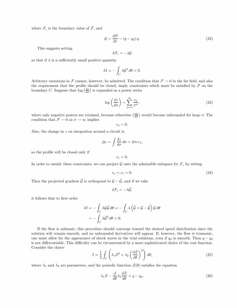
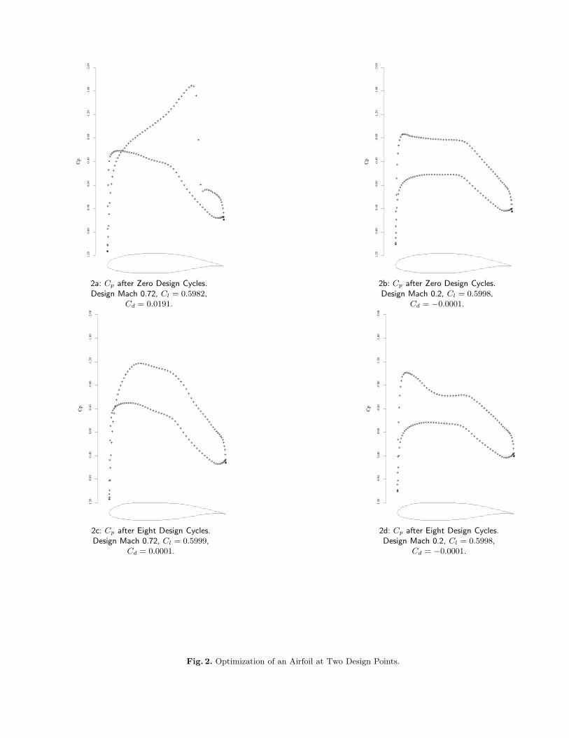
Fig. 2. Optimization of an Airfoil at Two Design Points.

to allow for a wedge angle ε at the trailing edge. The coefficients are determined by an iterative process withthe aid of fast Fourier transforms [23].

The adjoint equation has a form very similar to the flow equation. While it is linear in its dependentvariable, it also changes type from elliptic in subsonic zones of the flow to hyperbolic in supersonic zonesof the flow. Thus, it was possible to adapt exactly the same algorithm to solve both the adjoint and theflow equations, but with reverse biasing of the difference operators in the downwind direction in the adjointequation, corresponding to the reversed direction of the zone of dependence. The Poisson equation (21) issolved by the Buneman algorithm.

The efficiency of the present approach, which uses separate discretizations of the flow and adjoint equa-tions, depends on the fact that in the limit of zero mesh width the discrete adjoint solution converges tothe true adjoint solution. This allows the use of a rather simple discretization of the adjoint equation mod-eled after the discretization of the flow equation. Numerical experiments confirm that in practice separatediscretizations of the flow and adjoint equations yields good convergence to an optimum solution.

As an example of the application of the method, Figure 2 presents a calculation in which an airfoil wasredesigned to improve its transonic performance by reducing the pressure drag induced by the appearanceof a shock wave. The drag coefficient was therefore included in the cost function so that equation (25) isreplaced by

I =1

2

∫

C

(

λ1Z2 + λ2

(

dZ

dθ

)2)

dθ + λ3 Cd,

where λ3 is a parameter which may be varied to alter the trade-off between drag reduction and deviationfrom the desired pressure distribution. Representing the drag as

D =

∫

C

(p− p∞)dy

dθdθ,

the procedure of Section 3 may be used to determine the gradient by solving the adjoint equation witha modified boundary condition. A penalty on the desired pressure distribution is still needed to avoid asituation in which the optimum shape is a flat plate with no lift and no drag.

It was also desired to preserve the subsonic characteristics of the airfoil. Therefore two design pointswere specified, Mach 0.20 and Mach 0.720, and in each case the lift coefficient was forced to be 0.6. Thecomposite cost function was taken to be the sum of the values of the cost function at the two design points.The transonic drag coefficient was reduced from 0.0191 to 0.0001 in 8 design cycles. In order to achieve thisreduction the airfoil had to be modified so that its subsonic pressure distribution became more peaky at theleading edge. This is consistent with the results of experimental research on transonic airfoils, in which ithas generally been found necessary to have a peaky subsonic presure distribution in order to delay the onsetof the transonic drag rise. It is also important to control the adverse pressure gradient on the rear uppersurface, which can lead to premature separation of the viscous boundary layer. It can be seen that there isno steepening of this gradient due to the redesign.

4 The Navier-Stokes Equations

For the derivations that follow, it is convenient to use Cartesian coordinates (x1,x2,x3) and to adopt theconvention of indicial notation where a repeated index “i” implies summation over i = 1 to 3. The three-dimensional Navier-Stokes equations then take the form

∂w

∂t+∂fi

∂xi

=∂fvi

∂xi

in D, (30)

where the state vector w, inviscid flux vector f and viscous flux vector fv are described respectively by

w =

ρρu1

ρu2

ρu3

ρE

, fi =

ρui

ρuiu1 + pδi1ρuiu2 + pδi2ρuiu3 + pδi3

ρuiH

, fvi =

0σijδj1σijδj2σijδj3

ujσij + k ∂T∂xi

. (31)

In these definitions, ρ is the density, u1, u2, u3 are the Cartesian velocity components, E is the total energyand δij is the Kronecker delta function. The pressure is determined by the equation of state

p = (γ − 1) ρ

{

E −1

2(uiui)

}

,

and the stagnation enthalpy is given by

H = E +p

ρ,

where γ is the ratio of the specific heats. The viscous stresses may be written as

σij = µ

(

∂ui

∂xj

+∂uj

∂xi

)

+ λδij∂uk

∂xk

, (32)

where µ and λ are the first and second coefficients of viscosity. The coefficient of thermal conductivity andthe temperature are computed as

k =cpµ

Pr, T =

p

Rρ, (33)

where Pr is the Prandtl number, cp is the specific heat at constant pressure, and R is the gas constant.For discussion of real applications using a discretization on a body conforming structured mesh, it is also

useful to consider a transformation to the computational coordinates (ξ1,ξ2,ξ3) defined by the metrics

Kij =

[

∂xi

∂ξj

]

, J = det (K) , K−1ij =

[

∂ξi∂xj

]

.

The Navier-Stokes equations can then be written in computational space as

∂ (Jw)

∂t+∂ (Fi − Fvi)

∂ξi= 0 in D, (34)

where the inviscid and viscous flux contributions are now defined with respect to the computational cellfaces by Fi = Sijfj and Fvi = Sijfvj , and the quantity Sij = JK−1

ij represents the projection of the ξi cellface along the xj axis. In obtaining equation (34) we have made use of the property that

∂Sij

∂ξi= 0 (35)

which represents the fact that the sum of the face areas over a closed volume is zero, as can be readily verifiedby a direct examination of the metric terms.

5 Formulation of the Optimal Design Problem for the Navier-Stokes Equations

Aerodynamic optimization is based on the determination of the effect of shape modifications on some perfor-mance measure which depends on the flow. For convenience, the coordinates ξi describing the fixed compu-tational domain are chosen so that each boundary conforms to a constant value of one of these coordinates.Variations in the shape then result in corresponding variations in the mapping derivatives defined by Kij .

Suppose that the performance is measured by a cost function

I =

∫

B

M (w, S) dBξ +

∫

D

P (w, S) dDξ ,

containing both boundary and field contributions where dBξ and dDξ are the surface and volume elementsin the computational domain. In general, M and P will depend on both the flow variables w and the metricsS defining the computational space. The design problem is now treated as a control problem where theboundary shape represents the control function, which is chosen to minimize I subject to the constraints

defined by the flow equations (34). A shape change produces a variation in the flow solution δw and themetrics δS which in turn produce a variation in the cost function

δI =

∫

B

δM(w, S) dBξ +

∫

D

δP(w, S) dDξ. (36)

This can be split asδI = δII + δIII , (37)

with

δM = [Mw]I δw + δMII ,

δP = [Pw]I δw + δPII , (38)

where we continue to use the subscripts I and II to distinguish between the contributions associated withthe variation of the flow solution δw and those associated with the metric variations δS. Thus [Mw]I and[Pw]I represent ∂M

∂wand ∂P

∂wwith the metrics fixed, while δMII and δPII represent the contribution of the

metric variations δS to δM and δP .In the steady state, the constraint equation (53) specifies the variation of the state vector δw by

δR =∂

∂ξiδ (Fi − Fvi) = 0. (39)

Here, also, δR, δFi and δFvi can be split into contributions associated with δw and δS using the notation

δR = δRI + δRII

δFi = [Fiw]I δw + δFiII

δFvi = [Fviw]I δw + δFviII . (40)

The inviscid contributions are easily evaluated as

[Fiw]I = Sij

∂fi

∂w, δFviII = δSijfj .

The details of the viscous contributions are complicated by the additional level of derivatives in the stressand heat flux terms.

Multiplying by a co-state vector ψ, which will play an analogous role to the Lagrange multiplier introducedin equation (4), and integrating over the domain produces

∫

D

ψT ∂

∂ξiδ (Fi − Fvi) dDξ = 0. (41)

Assuming that ψ is differentiable the terms with subscript I may be integrated by parts to give

∫

B

niψT δ (Fi − Fvi)I dBξ −

∫

D

∂ψT

∂ξiδ (Fi − Fvi)I dDξ +

∫

D

ψT δRIIdDξ = 0. (42)

This equation results directly from taking the variation of the weak form of the flow equations, where ψ istaken to be an arbitrary differentiable test function. Since the left hand expression equals zero, it may besubtracted from the variation in the cost function (36) to give

δI = δIII −

∫

D

ψT δRIIdDξ −

∫

B

[

δMI − niψT δ (Fi − Fvi)I

]

dBξ

+

∫

D

[

δPI +∂ψT

∂ξiδ (Fi − Fvi)I

]

dDξ. (43)

Now, since ψ is an arbitrary differentiable function, it may be chosen in such a way that δI no longerdepends explicitly on the variation of the state vector δw. The gradient of the cost function can then be

evaluated directly from the metric variations without having to recompute the variation δw resulting fromthe perturbation of each design variable.

Comparing equations (38) and (40), the variation δw may be eliminated from (43) by equating all fieldterms with subscript “I” to produce a differential adjoint system governing ψ

∂ψT

∂ξi[Fiw − Fviw]I + [Pw]I = 0 in D. (44)

The corresponding adjoint boundary condition is produced by equating the subscript “I” boundary termsin equation (43) to produce

niψT [Fiw − Fviw]I = [Mw]I on B. (45)

The remaining terms from equation (43) then yield a simplified expression for the variation of the costfunction which defines the gradient

δI = δIII +

∫

D

ψT δRIIdDξ , (46)

which consists purely of the terms containing variations in the metrics with the flow solution fixed. Hencean explicit formula for the gradient can be derived once the relationship between mesh perturbations andshape variations is defined.

Comparing equations (38) and (40), the variation δw may be eliminated from (43) by equating all fieldterms with subscript “I” to produce a differential adjoint system governing ψ

∂ψT

∂ξi[Fiw − Fviw]I + Pw = 0 in D. (47)

The corresponding adjoint boundary condition is produced by equating the subscript “I” boundary termsin equation (43) to produce

niψT [Fiw − Fviw]I = Mw on B. (48)

The remaining terms from equation (43) then yield a simplified expression for the variation of the costfunction which defines the gradient

δI =

∫

B

{

δMII − niψT [δFi − δFvi] II

}

dBξ +

∫

D

{

δPII +∂ψT

∂ξi[δFi − δFvi] II

}

dDξ . (49)

The details of the formula for the gradient depend on the way in which the boundary shape is parameterized asa function of the design variables, and the way in which the mesh is deformed as the boundary is modified.Using the relationship between the mesh deformation and the surface modification, the field integral isreduced to a surface integral by integrating along the coordinate lines emanating from the surface. Thus theexpression for δI is finally reduced to the form of equation (6)

δI =

∫

B

GδF dBξ

where F represents the design variables, and G is the gradient, which is a function defined over the boundarysurface.

The boundary conditions satisfied by the flow equations restrict the form of the left hand side of theadjoint boundary condition (48). Consequently, the boundary contribution to the cost function M cannotbe specified arbitrarily. Instead, it must be chosen from the class of functions which allow cancellation ofall terms containing δw in the boundary integral of equation (43). On the other hand, there is no suchrestriction on the specification of the field contribution to the cost function P , since these terms may alwaysbe absorbed into the adjoint field equation (47) as source terms.

It is convenient to develop the inviscid and viscous contributions to the adjoint equations separately. Also,for simplicity, it will be assumed that the portion of the boundary that undergoes shape modifications isrestricted to the coordinate surface ξ2 = 0. Then equations (43) and (45) may be simplified by incorporatingthe conditions

n1 = n3 = 0, n2 = 1, dBξ = dξ1dξ3,

so that only the variations δF2 and δFv2 need to be considered at the wall boundary.

6 Derivation of the Inviscid Adjoint Terms

The inviscid contributions have been previously derived in [13,25] but are included here for completeness.Taking the transpose of equation (44), the inviscid adjoint equation may be written as

CTi

∂ψ

∂ξi= 0 in D, (50)

where the inviscid Jacobian matrices in the transformed space are given by

Ci = Sij

∂fj

∂w.

The transformed velocity components have the form

Ui = Sijuj ,

and the condition that there is no flow through the wall boundary at ξ2 = 0 is equivalent to

U2 = 0,

so thatδU2 = 0

when the boundary shape is modified. Consequently the variation of the inviscid flux at the boundary reducesto

δF2 = δp

0

S21

S22

S23

0

+ p

0

δS21

δS22

δS23

0

. (51)

Since δF2 depends only on the pressure, it is now clear that the performance measure on the boundaryM(w, S) may only be a function of the pressure and metric terms. Otherwise, complete cancellation of theterms containing δw in the boundary integral would be impossible. One may, for example, include arbitrarymeasures of the forces and moments in the cost function, since these are functions of the surface pressure.

In order to design a shape which will lead to a desired pressure distribution, a natural choice is to set

I =1

2

∫

B

(p− pd)2dS

where pd is the desired surface pressure, and the integral is evaluated over the actual surface area. In thecomputational domain this is transformed to

I =1

2

∫ ∫

Bw

(p− pd)2 |S2| dξ1dξ3,

where the quantity|S2| =

√

S2jS2j

denotes the face area corresponding to a unit element of face area in the computational domain. Now, tocancel the dependence of the boundary integral on δp, the adjoint boundary condition reduces to

ψjnj = p− pd (52)

where nj are the components of the surface normal

nj =S2j

|S2|.

This amounts to a transpiration boundary condition on the co-state variables corresponding to the momen-tum components. Note that it imposes no restriction on the tangential component of ψ at the boundary.

In the presence of shock waves, neither p nor pd are necessarily continuous at the surface. The boundarycondition is then in conflict with the assumption that ψ is differentiable. This difficulty can be circumventedby the use of a smoothed boundary condition [25].

7 Derivation of the Viscous Adjoint Terms

In computational coordinates, the viscous terms in the Navier–Stokes equations have the form

∂Fvi

∂ξi=

∂

∂ξi

(

Sijfvj

)

.

Computing the variation δw resulting from a shape modification of the boundary, introducing a co-statevector ψ and integrating by parts following the steps outlined by equations (39) to (42) produces

∫

B

ψT(

δS2jfvj + S2jδfvj

)

dBξ −

∫

D

∂ψT

∂ξi

(

δSijfvj + Sijδfvj

)

dDξ ,

where the shape modification is restricted to the coordinate surface ξ2 = 0 so that n1 = n3 = 0, and n2 = 1.Furthermore, it is assumed that the boundary contributions at the far field may either be neglected or elseeliminated by a proper choice of boundary conditions as previously shown for the inviscid case [13,25].

The viscous terms will be derived under the assumption that the viscosity and heat conduction coefficientsµ and k are essentially independent of the flow, and that their variations may be neglected. This simplificationhas been successfully used for may aerodynamic problems of interest. In the case of some turbulent flows,there is the possibility that the flow variations could result in significant changes in the turbulent viscosity,and it may then be necessary to account for its variation in the calculation.

Transformation to Primitive Variables

The derivation of the viscous adjoint terms is simplified by transforming to the primitive variables

wT = (ρ, u1, u2, u3, p)T ,

because the viscous stresses depend on the velocity derivatives ∂ui

∂xj, while the heat flux can be expressed as

κ∂

∂xi

(

p

ρ

)

.

where κ = kR

= γµPr(γ−1) . The relationship between the conservative and primitive variations is defined by

the expressionsδw = Mδw, δw = M−1δw

which make use of the transformation matrices M = ∂w∂w

and M−1 = ∂w∂w

. These matrices are provided intransposed form for future convenience

MT =

1 u1 u2 u3uiui

20 ρ 0 0 ρu1

0 0 ρ 0 ρu2

0 0 0 ρ ρu3

0 0 0 0 1γ−1

M−1T=

1 −u1

ρ−u2

ρ−u3

ρ

(γ−1)uiui

2

0 1ρ

0 0 −(γ − 1)u1

0 0 1ρ

0 −(γ − 1)u2

0 0 0 1ρ

−(γ − 1)u3

0 0 0 0 γ − 1

.

The conservative and primitive adjoint operators L and L corresponding to the variations δw and δw arethen related by

∫

D

δwTLψ dDξ =

∫

D

δwT Lψ dDξ ,

withL = MTL,

so that after determining the primitive adjoint operator by direct evaluation of the viscous portion of (44),

the conservative operator may be obtained by the transformation L = M−1TL. Since the continuity equation

contains no viscous terms, it makes no contribution to the viscous adjoint system. Therefore, the derivationproceeds by first examining the adjoint operators arising from the momentum equations.

Contributions from the Momentum Equations

In order to make use of the summation convention, it is convenient to set ψj+1 = φj for j = 1, 2, 3. Thenthe contribution from the momentum equations is

∫

B

φk (δS2jσkj + S2jδσkj) dBξ−

∫

D

∂φk

∂ξi(δSijσkj + Sijδσkj) dDξ . (53)

The velocity derivatives in the viscous stresses can be expressed as

∂ui

∂xj

=∂ui

∂ξl

∂ξl∂xj

=Slj

J

∂ui

∂ξl

with corresponding variations

δ∂ui

∂xj

=

[

Slj

J

]

I

∂

∂ξlδui +

[

∂ui

∂ξl

]

II

δ

(

Slj

J

)

.

The variations in the stresses are then

δσkj ={

µ[

Slj

J∂

∂ξlδuk + Slk

J∂

∂ξlδuj

]

+ λ[

δjkSlm

J∂

∂ξlδum

]}

I

+{

µ[

δ(

Slj

J

)

∂uk

∂ξl+ δ

(

Slk

J

) ∂uj

∂ξl

]

+ λ[

δjkδ(

Slm

J

)

∂um

∂ξl

]}

II.

As before, only those terms with subscript I , which contain variations of the flow variables, need be consideredfurther in deriving the adjoint operator. The field contributions that contain δui in equation (53) appear as

−

∫

D

∂φk

∂ξiSij

{

µ

(

Slj

J

∂

∂ξlδuk +

Slk

J

∂

∂ξlδuj

)

+λδjk

Slm

J

∂

∂ξlδum

}

dDξ.

This may be integrated by parts to yield

∫

D

δuk

∂

∂ξl

(

SljSij

µ

J

∂φk

∂ξi

)

dDξ

+

∫

D

δuj

∂

∂ξl

(

SlkSij

µ

J

∂φk

∂ξi

)

dDξ

+

∫

D

δum

∂

∂ξl

(

SlmSij

λδjk

J

∂φk

∂ξi

)

dDξ,

where the boundary integral has been eliminated by noting that δui = 0 on the solid boundary. By exchangingindices, the field integrals may be combined to produce

∫

D

δuk

∂

∂ξlSlj

{

µ

(

Sij

J

∂φk

∂ξi+Sik

J

∂φj

∂ξi

)

+ λδjk

Sim

J

∂φm

∂ξi

}

dDξ ,

which is further simplified by transforming the inner derivatives back to Cartesian coordinates

∫

D

δuk

∂

∂ξlSlj

{

µ

(

∂φk

∂xj

+∂φj

∂xk

)

+ λδjk

∂φm

∂xm

}

dDξ . (54)

The boundary contributions that contain δui in equation (53) may be simplified using the fact that

∂

∂ξlδui = 0 if l = 1, 3

on the boundary B so that they become

∫

B

φkS2j

{

µ

(

S2j

J

∂

∂ξ2δuk +

S2k

J

∂

∂ξ2δuj

)

+ λδjk

S2m

J

∂

∂ξ2δum

}

dBξ. (55)

Together, (54) and (55) comprise the field and boundary contributions of the momentum equations to theviscous adjoint operator in primitive variables.

Contributions from the Energy Equation

In order to derive the contribution of the energy equation to the viscous adjoint terms it is convenient to set

ψ5 = θ, Qj = uiσij + κ∂

∂xj

(

p

ρ

)

,

where the temperature has been written in terms of pressure and density using (33). The contribution fromthe energy equation can then be written as

∫

B

θ (δS2jQj + S2jδQj) dBξ −

∫

D

∂θ

∂ξi(δSijQj + SijδQj) dDξ . (56)

The field contributions that contain δui,δp, and δρ in equation (56) appear as

−

∫

D

∂θ

∂ξiSijδQjdDξ = −

∫

D

∂θ

∂ξiSij

{

δukσkj + ukδσkj +κSlj

J

∂

∂ξl

(

δp

ρ−p

ρ

δρ

ρ

)}

dDξ. (57)

The term involving δσkj may be integrated by parts to produce

∫

D

δuk

∂

∂ξlSlj

{

µ

(

uk

∂θ

∂xj

+ uj

∂θ

∂xk

)

+λδjkum

∂θ

∂xm

}

dDξ , (58)

where the conditions ui = δui = 0 are used to eliminate the boundary integral on B. Notice that the otherterm in (57) that involves δuk need not be integrated by parts and is merely carried on as

−

∫

D

δukσkjSij

∂θ

∂ξidDξ (59)

The terms in expression (57) that involve δp and δρ may also be integrated by parts to produce both afield and a boundary integral. The field integral becomes

∫

D

(

δp

ρ−p

ρ

δρ

ρ

)

∂

∂ξl

(

SljSij

κ

J

∂θ

∂ξi

)

dDξ

which may be simplified by transforming the inner derivative to Cartesian coordinates

∫

D

(

δp

ρ−p

ρ

δρ

ρ

)

∂

∂ξl

(

Sljκ∂θ

∂xj

)

dDξ . (60)

The boundary integral becomes

∫

B

κ

(

δp

ρ−p

ρ

δρ

ρ

)

S2jSij

J

∂θ

∂ξidBξ. (61)

This can be simplified by transforming the inner derivative to Cartesian coordinates

∫

B

κ

(

δp

ρ−p

ρ

δρ

ρ

)

S2j

J

∂θ

∂xj

dBξ, (62)

and identifying the normal derivative at the wall

∂

∂n= S2j

∂

∂xj

, (63)

and the variation in temperature

δT =1

R

(

δp

ρ−p

ρ

δρ

ρ

)

,

to produce the boundary contribution∫

B

kδT∂θ

∂ndBξ. (64)

This term vanishes if T is constant on the wall but persists if the wall is adiabatic.There is also a boundary contribution left over from the first integration by parts (56) which has the

form∫

B

θδ (S2jQj) dBξ, (65)

where

Qj = k∂T

∂xj

,

since ui = 0. Notice that for future convenience in discussing the adjoint boundary conditions resulting fromthe energy equation, both the δw and δS terms corresponding to subscript classes I and II are consideredsimultaneously. If the wall is adiabatic

∂T

∂n= 0,

so that using (63),

δ (S2jQj) = 0,

and both the δw and δS boundary contributions vanish.On the other hand, if T is constant ∂T

∂ξl= 0 for l = 1, 3, so that

Qj = k∂T

∂xj

= k

(

Slj

J

∂T

∂ξl

)

= k

(

S2j

J

∂T

∂ξ2

)

.

Thus, the boundary integral (65) becomes

∫

B

kθ

{

S2j2

J

∂

∂ξ2δT + δ

(

S2j2

J

)

∂T

∂ξ2

}

dBξ . (66)

Therefore, for constant T , the first term corresponding to variations in the flow field contributes to theadjoint boundary operator and the second set of terms corresponding to metric variations contribute to thecost function gradient.

All together, the contributions from the energy equation to the viscous adjoint operator are the threefield terms (58), (59) and (60), and either of two boundary contributions ( 64) or ( 66), depending on whetherthe wall is adiabatic or has constant temperature.

The Viscous Adjoint Field Operator

Collecting together the contributions from the momentum and energy equations, the viscous adjoint operatorin primitive variables can be expressed as

(Lψ)1 = − pρ2

∂∂ξl

(

Sljκ∂θ∂xj

)

(Lψ)i+1 = ∂∂ξl

{

Slj

[

µ(

∂φi

∂xj+

∂φj

∂xi

)

+ λδij∂φk

∂xk

]}

+ ∂∂ξl

{

Slj

[

µ(

ui∂θ∂xj

+ uj∂θ∂xi

)

+ λδijuk∂θ

∂xk

]}

for i = 1, 2, 3

− σijSlj∂θ∂ξl

(Lψ)5 = 1ρ

∂∂ξl

(

Sljκ∂θ∂xj

)

.

The conservative viscous adjoint operator may now be obtained by the transformation

L = M−1TL.

8 Viscous Adjoint Boundary Conditions

It was recognized in Section 5 that the boundary conditions satisfied by the flow equations restrict the formof the performance measure that may be chosen for the cost function. There must be a direct correspondencebetween the flow variables for which variations appear in the variation of the cost function, and those variablesfor which variations appear in the boundary terms arising during the derivation of the adjoint field equations.Otherwise it would be impossible to eliminate the dependence of δI on δw through proper specification ofthe adjoint boundary condition. As in the derivation of the field equations, it proves convenient to considerthe contributions from the momentum equations and the energy equation separately.

Boundary Conditions Arising from the Momentum Equations

The boundary term that arises from the momentum equations including both the δw and δS components(53) takes the form

∫

B

φkδ (S2jσkj) dBξ .

Replacing the metric term with the corresponding local face area S2 and unit normal nj defined by

|S2| =√

S2jS2j , nj =S2j

|S2|

then leads to∫

B

φkδ (|S2|njσkj) dBξ.

Defining the components of the surface stress as

τk = njσkj

and the physical surface elementdS = |S2| dBξ,

the integral may then be split into two components∫

B

φkτk |δS2| dBξ +

∫

B

φkδτkdS, (67)

where only the second term contains variations in the flow variables and must consequently cancel the δwterms arising in the cost function. The first term will appear in the expression for the gradient.

A general expression for the cost function that allows cancellation with terms containing δτk has the form

I =

∫

B

N (τ)dS, (68)

corresponding to a variation

δI =

∫

B

∂N

∂τkδτkdS,

for which cancellation is achieved by the adjoint boundary condition

φk =∂N

∂τk.

Natural choices for N arise from force optimization and as measures of the deviation of the surface stressesfrom desired target values.

For viscous force optimization, the cost function should measure friction drag. The friction force in thexi direction is

CDfi =

∫

B

σijdSj =

∫

B

S2jσijdBξ

so that the force in a direction with cosines qi has the form

Cqf =

∫

B

qiS2jσijdBξ.

Expressed in terms of the surface stress τi, this corresponds to

Cqf =

∫

B

qiτidS,

so that basing the cost function (68) on this quantity gives

N = qiτi.

Cancellation with the flow variation terms in equation (67) therefore mandates the adjoint boundary condi-tion

φk = nk.

Note that this choice of boundary condition also eliminates the first term in equation (67) so that it neednot be included in the gradient calculation.

In the inverse design case, where the cost function is intended to measure the deviation of the surfacestresses from some desired target values, a suitable definition is

N (τ) =1

2alk (τl − τdl) (τk − τdk) ,

where τd is the desired surface stress, including the contribution of the pressure, and the coefficients alk

define a weighting matrix. For cancellation

φkδτk = alk (τl − τdl) δτk.

This is satisfied by the boundary condition

φk = alk (τl − τdl) . (69)

Assuming arbitrary variations in δτk, this condition is also necessary.In order to control the surface pressure and normal stress one can measure the difference

nj {σkj + δkj (p− pd)} ,

where pd is the desired pressure. The normal component is then

τn = nknjσkj + p− pd,

so that the measure becomes

N (τ) =1

2τ2n

=1

2nlnmnknj {σlm + δlm (p− pd)} {σkj + δkj (p− pd)} .

This corresponds to settingalk = nlnk

in equation (69). Defining the viscous normal stress as

τvn = nknjσkj ,

the measure can be expanded as

N (τ) =1

2nlnmnknjσlmσkj +

1

2(nknjσkj + nlnmσlm) (p− pd) +

1

2(p− pd)

2

=1

2τ2vn + τvn (p− pd) +

1

2(p− pd)

2.

For cancellation of the boundary terms

φk (njδσkj + nkδp) ={

nlnmσlm + n2l (p− pd)

}

nk (njδσkj + nkδp)

leading to the boundary conditionφk = nk (τvn + p− pd) .

In the case of high Reynolds number, this is well approximated by the equations

φk = nk (p− pd) , (70)

which should be compared with the single scalar equation derived for the inviscid boundary condition (52).In the case of an inviscid flow, choosing

N (τ) =1

2(p− pd)

2

requiresφknkδp = (p− pd)n

2kδp = (p− pd) δp

which is satisfied by equation (70), but which represents an overspecification of the boundary condition sinceonly the single condition (52) need be specified to ensure cancellation.

Boundary Conditions Arising from the Energy Equation

The form of the boundary terms arising from the energy equation depends on the choice of temperatureboundary condition at the wall. For the adiabatic case, the boundary contribution is (64)

∫

B

kδT∂θ

∂ndBξ,

while for the constant temperature case the boundary term is (66). One possibility is to introduce a contri-bution into the cost function which depends on T or ∂T

∂nso that the appropriate cancellation would occur.

Since there is little physical intuition to guide the choice of such a cost function for aerodynamic design, amore natural solution is to set

θ = 0

in the constant temperature case or∂θ

∂n= 0

in the adiabatic case. Note that in the constant temperature case, this choice of θ on the boundary wouldalso eliminate the boundary metric variation terms in (65).

9 Implementation of Navier-Stokes Design

The design procedures can be summarized as follows:

1. Solve the flow equations for ρ, u1, u2, u3, p.2. Solve the adjoint equations for ψ subject to appropriate boundary conditions.3. Evaluate G .4. Project G into an allowable subspace that satisfies any geometric constraints.5. Update the shape based on the direction of steepest descent.6. Return to 1 until convergence is reached.

Practical implementation of the viscous design method relies heavily upon fast and accurate solvers for boththe state (w) and co-state (ψ) systems. This work uses well-validated software for the solution of the Eulerand Navier-Stokes equations developed over the course of many years [26–28].

For inverse design the lift is fixed by the target pressure. In drag minimization it is also appropriate to fixthe lift coefficient, because the induced drag is a major fraction of the total drag, and this could be reducedsimply by reducing the lift. Therefore the angle of attack is adjusted during the flow solution to force aspecified lift coefficient to be attained, and the influence of variations of the angle of attack is included in thecalculation of the gradient. The vortex drag also depends on the span loading, which may be constrained byother considerations such as structural loading or buffet onset. Consequently, the option is provided to forcethe span loading by adjusting the twist distribution as well as the angle of attack during the flow solution.

Discretization

Both the flow and the adjoint equations are discretized using a semi-discrete cell-centered finite volumescheme. The convective fluxes across cell interfaces are represented by simple arithmetic averages of thefluxes computed using values from the cells on either side of the face, augmented by artificial diffusive termsto prevent numerical oscillations in the vicinity of shock waves. Continuing to use the summation conventionfor repeated indices, the numerical convective flux across the interface between cells A and B in a threedimensional mesh has the form

hAB =1

2SABj

(

fAj+ fBj

)

− dAB ,

where SABjis the component of the face area in the jth Cartesian coordinate direction,

(

fAj

)

and(

fBj

)

denote the flux fj as defined by equation (12) and dAB is the diffusive term. Variations of the computerprogram provide options for alternate constructions of the diffusive flux.

The simplest option implements the Jameson-Schmidt-Turkel scheme [26,29], using scalar diffusive termsof the form

dAB = ε(2)∆w − ε(4)(

∆w+ − 2∆w +∆w−)

,

where∆w = wB − wA

and ∆w+ and ∆w− are the same differences across the adjacent cell interfaces behind cell A and beyondcell B in the AB direction. By making the coefficient ε(2) depend on a switch proportional to the undividedsecond difference of a flow quantity such as the pressure or entropy, the diffusive flux becomes a third orderquantity, proportional to the cube of the mesh width in regions where the solution is smooth. Oscillations aresuppressed near a shock wave because ε(2) becomes of order unity, while ε(4) is reduced to zero by the sameswitch. For a scalar conservation law, it is shown in reference [29] that ε(2) and ε(4) can be constructed tomake the scheme satisfy the local extremum diminishing (LED) principle that local maxima cannot increasewhile local minima cannot decrease.

The second option applies the same construction to local characteristic variables. There are derived fromthe eigenvectors of the Jacobian matrix AAB which exactly satisfies the relation

AAB (wB − wA) = SABj

(

fBj− fAj

)

.

This corresponds to the definition of Roe [30]. The resulting scheme is LED in the characteristic variables.The third option implements the H-CUSP scheme proposed by Jameson [31] which combines differences

fB − fA and wB − wA in a manner such that stationary shock waves can be captured with a single interiorpoint in the discrete solution. This scheme minimizes the numerical diffusion as the velocity approaches zeroin the boundary layer, and has therefore been preferred for viscous calculations in this work.

Similar artificial diffusive terms are introduced in the discretization of the adjoint equation, but withthe opposite sign because the wave directions are reversed in the adjoint equation. Satisfactory results havebeen obtained using scalar diffusion in the adjoint equation while characteristic or H-CUSP constructionsare used in the flow solution.

i jσ

dual cell

Fig. 3. Cell-centered scheme. σij evaluated at vertices of the primary mesh

The discretization of the viscous terms of the Navier Stokes equations requires the evaluation of the

velocity derivatives∂ui

∂xj

in order to calculate the viscous stress tensor σij defined in equation (32). These

are most conveniently evaluated at the cell vertices of the primary mesh by introducing a dual mesh whichconnects the cell centers of the primary mesh, as depicted in Figure (3). According to the Gauss formula fora control volume V with boundary S

∫

V

∂vi

∂xj

dv =

∫

S

uinjdS

where nj is the outward normal. Applied to the dual cells this yields the estimate

∂vi

∂xj

=1

vol

∑

faces

uinjS

where S is the area of a face, and ui is an estimate of the average of ui over that face. In order to determinethe viscous flux balance of each primary cell, the viscous flux across each of its faces is then calculated fromthe average of the viscous stress tensor at the four vertices connected by that face. This leads to a compactscheme with a stencil connecting each cell to its 26 nearest neighbors.

The semi-discrete schemes for both the flow and the adjoint equations are both advanced to steady stateby a multi-stage time stepping scheme. This is a generalized Runge-Kutta scheme in which the convective anddiffusive terms are treated differently to enlarge the stability region [29,32]. Convergence to a steady state isaccelerated by residual averaging and a multi-grid procedure [33]. These algorithms have been implementedboth for single and multiblock meshes and for operation on parallel computers with message passing usingthe MPI (Message Passing Interface) protocol [9,34,35].

In this work, the adjoint and flow equations are discretized separately. The alternative approach ofderiving the discrete adjoint equations directly from the discrete flow equations yields another possible

discretization of the adjoint partial differential equation which is more complex. If the resulting equationswere solved exactly, they could provide the exact gradient of the inexact cost function which results from thediscretization of the flow equations. On the other hand, any consistent discretization of the adjoint partialdifferential equation will yield the exact gradient as the mesh is refined, and separate discretization hasproved to work perfectly well in practice. It should also be noted that the discrete gradient includes bothmesh effects and numerical errors such as spurious entropy production which may not reflect the true costfunction of the continuous problem.

Mesh Generation and Geometry Control

Meshes for both viscous optimization and for the treatment of complex configurations are externally gen-erated in order to allow for their inspection and careful quality control. Single block meshes with a C-Htopology have been used for viscous optimization of wing-body combinations, while multiblock meshes havebeen generated for complex configurations using GRIDGEN [36]. In either case geometry modifications areaccommodated by a grid perturbation scheme. For viscous wing-body design using single block meshes, thewing surface mesh points themselves are taken as the design variables. A simple mesh perturbation schemeis then used, in which the mesh points lying on a mesh line projecting out from the wing surface are allshifted in the same sense as the surface mesh point, with a decay factor proportional to the arc length alongthe mesh line. The resulting perturbation in the face areas of the neighboring cells are then included inthe gradient calculation. For complex configurations the geometry is controlled by superposition of analytic“bump” functions defined over the surfaces which are to be modified. The grid is then perturbed to conformto modifications of the surface shape by the WARP3D and WARP-MB algorithms described in [34].

Optimization

Two main search procedures have been used in our applications to date. The first is a simple descent methodin which small steps are taken in the negative gradient direction. Let F represent the design variable, and Gthe gradient. Then the iteration

δF = −λG

can be regarded as simulating the time dependent process

dF

dt= −G

where λ is the time step ∆t. Let A be the Hessian matrix with elements

Aij =∂Gi

∂Fj

=∂2I

∂Fi∂Fj

.

Suppose that a locally minimum value of the cost function I∗ = I(F∗) is attained when F = F∗. Then thegradient G∗ = G(F∗) must be zero, while the Hessian matrix A∗ = A(F∗) must be positive definite. SinceG∗ is zero, the cost function can be expanded as a Taylor series in the neighborhood of F ∗ with the form

I(F) = I∗ +1

2(F −F∗)A (F −F∗) + . . .

Correspondingly,G(F) = A (F −F∗) + . . .

As F approaches F∗, the leading terms become dominant. Then, setting F = (F −F∗), the search processapproximates

dF

dt= −A∗F .

Also, since A∗ is positive definite it can be expanded as

A∗ = RMRT ,

where M is a diagonal matrix containing the eigenvalues of A∗, and

RRT = RTR = I.

Settingv = RT F ,

the search process can be represented asdv

dt= −Mv.

The stability region for the simple forward Euler stepping scheme is a unit circle centered at −1 on thenegative real axis. Thus for stability we must choose

µmax∆t = µmaxλ < 2,

while the asymptotic decay rate, given by the smallest eigenvalue, is proportional to

e−µmint.

In order to make sure that each new shape in the optimization sequence remains smooth, it provesessential to smooth the gradient and to replace G by its smoothed value G in the descent process. This alsoacts as a preconditioner which allows the use of much larger steps. To apply smoothing in the ξ1 direction,for example, the smoothed gradient G may be calculated from a discrete approximation to

G −∂

∂ξ1ε∂

∂ξ1G = G (71)

where ε is the smoothing parameter. If one sets δF = −λG, then, assuming the modification is applied onthe surface ξ2 = constant, the first order change in the cost function is

δI = −

∫ ∫

GδF dξ1dξ3

= −λ

∫ ∫(

G −∂

∂ξ1ε∂G

∂ξ1

)

G dξ1dξ3

= −λ

∫ ∫

(

G2 + ε

(

∂G

∂ξ1

)2)

dξ1dξ3

< 0,

assuring an improvement if λ is sufficiently small and positive, unless the process has already reached astationary point at which G = 0.

It turns out that this approach is tolerant to the use of approximate values of the gradient, so thatneither the flow solution nor the adjoint solution need be fully converged before making a shape change.This results in very large savings in the computational cost. For inviscid optimization it is necessary to useonly 15 multigrid cycles for the flow solution and the adjoint solution in each design iteration. For viscousoptimization, about 20-30 multigrid cycles are needed.

Our second main search procedure incorporates a quasi-Newton method for general constrained opti-mization. In this class of methods the step is defined as

δF = −λPG,

where P is a preconditioner for the search. An ideal choice is P = A∗−1, so that the corresponding timedependent process reduces to

dF

dt= −F ,

for which all the eigenvalues are equal to unity, and F is reduced to zero in one time step by the choice∆t = 1 if the Hessian, A, is constant. The full Newton method takes P = A−1, requiring the evaluation of the

Hessian matrix, A, at each step. It corresponds to the use of the Newton-Raphson method to solve the non-linear equation G = 0. Quasi-Newton methods estimate A∗ from the change in the gradient during the searchprocess. This requires accurate estimates of the gradient at each time step. In order to obtain these, boththe flow solution and the adjoint equation must be fully converged. Most quasi-Newton methods also requirea line search in each search direction, for which the flow equations and cost function must be accuratelyevaluated several times. They have proven quite robust in practice for aerodynamic optimization [37].

In the applications to complex configurations presented below the optimization was carried out usingthe existing, well validated software NPSOL. This software, which implements a quasi-Newton method foroptimization with both linear and non-linear constraints, has proved very reliable but is generally moreexpensive than the simple search method with smoothing.

10 Industrial Experience and Results

The methods described in this paper have been quite thoroughly tested in industrial applications in whichthey were used as a tool for aerodynamic design. They have proved useful both in inverse mode to findshapes that would produce desired pressure distributions, and for direct minimization of the drag. Theyhave been applied both to well understood configurations that have gradually evolved through incrementalimprovements guided by wind tunnel tests and computational simulation, and to new concepts for whichthere is a limited knowledge base. In either case they have enabled engineers to produce improved designs.

Substantial improvements are usually obtained with 20−200 design cycles, depending on the difficulty ofthe case. One concern is the possibility of getting trapped in a local minimum. In practice this has not provedto be a source of difficulty. In inverse mode, it often proves possible to come very close to realizing the targetpressure distribution, thus effectively demonstrating convergence. In drag minimization, the result of theoptimization is usually a shock-free wing. If one considers drag minimization of airfoils in two-dimensionalinviscid transonic flow, it can be seen that every shock-free airfoil produces zero drag, and thus optimizationbased solely on drag has a highly non-unique solution. Different shock-free airfoils can be obtained by startingfrom different initial profiles. One may also influence the character of the final design by blending a targetpressure distribution with the drag in the definition of the cost function.

Similar considerations apply to three-dimensional wing design. Since the vortex drag can be reducedsimply by reducing the lift, the lift coefficient must be fixed for a meaningful drag minimization. In orderto do this the angle of attack α is adjusted during the flow solution. It has proved most effective to makea small change δα proportional to the difference between the actual and the desired lift coefficient at everyiteration in the flow calculation. A typical wing of a transport aircraft is designed for a lift coefficient inthe range of 0.4 to 0.6. The total wing drag may be broken down into vortex drag, drag due to viscouseffects, and shock drag. The vortex drag coefficient is typically in the range of 0.0100 (100 counts), whilethe friction drag coefficient is in the range of 45 counts, and the shock drag at a Mach number just beforethe onset of severe drag rise is of the order of 15 counts. With a fixed span, typically dictated by structurallimits or a constraint imposed by airport gates, the vortex drag is entirely a function of span loading, and isminimized by an elliptic loading unless winglets are added. Transport aircraft usually have highly taperedwings with very large root chords to accommodate retraction of the undercarriage. An elliptic loading maylead to excessively large section lift coefficients on the outboard wing, leading to premature shock stall orbuffet when the load is increased. The structure weight is also reduced by a more inboard loading whichreduces the root bending moment. Thus the choice of span loading is influenced by other considerations. Theskin friction of transport aircraft is typically very close to flat plate skin friction in turbulent flow, and is veryinsensitive to section variations. An exception to this is the case of smaller executive jet aircraft, for whichthe Reynolds number may be small enough to allow a significant run of laminar flow if the suction peakof the pressure distribution is moved back on the section. This leaves the shock drag as the primary targetfor wing section optimization. This is reduced to zero if the wing is shock-free, leaving no room for furtherimprovement. Thus the attainment of a shock-free flow is a demonstration of a successful drag minimization.In practice range is maximized by maximizing M L

D, and this is likely to be increased by increasing the lift

coefficient to the point where a weak shock appears. One may also use optimization to find the maximumMach number at which the shock drag can be eliminated or significantly reduced for a wing with a givensweepback angle and thickness. Alternatively one may try to find the largest wing thickness or the minimumsweepback angle for which the shock drag can be eliminated at a given Mach number. This can yield both

savings in structure weight and increased fuel volume . If there is no fixed limit for the wing span, such asa gate constraint, increased thickness can be used to allow an increase in aspect ratio for a wing of equalweight, in turn leading to a reduction in vortex drag. Since the vortex drag is usually the largest componentof the total wing drag, this is probably the most effective design strategy, and it may pay to increase thewing thickness to the point where the optimized section produces a weak shock wave rather than a shock-freeflow [25].

The first major industrial application of an adjoint based aerodynamic optimization method was thewing design of the Beech Premier [38] in 1995. The method was successfully used in inverse mode as a toolto obtain pressure distributions favorable to the maintenance of natural laminar flow over a range of cruiseMach numbers. Wing contours were obtained which yielded the desired pressure distribution in the presenceof closely coupled engine nacelles on the fuselage above the wing trailing edge.

During 1996 some preliminary studies indicated that the wings of both the McDonnell Douglas MD-11and the Boeing 747-200 could be made shock-free in a representative cruise condition by using very smallshape modifications, with consequent drag savings which could amount to several percent of the total drag.This led to a decision to evaluate adjoint-based design methods in the design of the McDonnell DouglasMDXX during the summer and fall of 1996. In initial studies wing redesigns were carried out for inviscidtransonic flow modeled by the Euler equations. A redesign to minimize the drag at a specified lift and Machnumber required about 40 design cycles, which could be completed overnight on a workstation.

Three main lessons were drawn from these initial studies: (i) the fuselage effect is to large to be ignoredand must be included in the optimization, (ii) single-point designs could be too sensitive to small variationsin the flight condition, typically producing a shock-free flow at the design point with a tendency to break upinto a severe double shock pattern below the design point, and (iii) the shape changes necessary to optimizea wing in transonic flow are smaller than the boundary layer displacement thickness, with the consequencethat viscous effects must be included in the final design.

In order to meet the first two of these considerations, the second phase of the study was concentratedon the optimization of wing-body combinations with multiple design points. These were still performed withinviscid flow to reduce computational cost and allow for fast turnaround. It was found that comparativelyinsensitive designs could be obtained by minimizing the drag at a fixed Mach number for three fairly closelyspaced lift coefficients such as 0.5, 0.525, and 0.55, or alternatively three nearby Mach numbers with a fixedlift coefficient.

The third phase of the project was focused on the design with viscous effects using as a starting pointwings which resulted from multipoint inviscid optimization. While the full viscous adjoint method was stillunder development, it was found that useful improvements could be realized, particularly in inverse mode,using the inviscid result to provide the target pressure, by coupling an inviscid adjoint solver to a viscousflow solver. Computer costs are many times larger, both because finer meshes are needed to resolve theboundary layer, and because more iterations are needed in the flow and adjoint solutions. In order to forcethe specified lift coefficient the number of iterations in each flow solution had to be increased from 15 to100. To achieve overnight turnaround a fully parallel implementation of the software had to be developed.Finally it was found that in order to produce sufficiently accurate results, the number of mesh points had tobe increased to about 1.8 million. In the final phase of this project it was planned to carry out a propulsionintegration study using the multiblock versions of the software. This study was not completed due to thecancellation of the entire MDXX project.

In the next subsections we present examples of the use of the adjoint method for viscous inverse anddrag minimization in two dimensional flow. We then show a three-dimensional wing design using the Eulerequations and a wing design using the full viscous adjoint method in its current form, implemented in thecomputer program SYN107. These calculations were all performed using the simple descent method withsmoothing of the gradient. This has proved to be very efficient: in all cases the final optimum design wasachieved with a total computational cost equivalent to the cost of from 2 to 10 converged flow solutions. Theremaining subsections present results of optimizations for complete configurations in inviscid transonic andsupersonic flow using the multiblock parallel design program, SYN107-MB.

Inverse design of an airfoil in transonic viscous flow

Our first example shows an inverse design in two dimensional viscous transonic flow obtained using thetwo-dimensional design code SYN103. The target pressure is that of the section of the ONERA M6 wingat Mach .75 and a lift coefficient of .50. It was calculated using SYN103 in analysis mode, thus it shouldbe exactly realizable. A C-type mesh was used which contained 256 intervals in the chordwise and 96 cellsin the normal direction for a total of 24, 576 cells. The design calculation was started with the NACA 0012airfoil as the initial profile, and the ONERA M6 pressure distribution was almost exactly recovered in 25design cycles. In the first cycle 120 iterations were used in both the flow and the adjoint solutions. In thesubsequent cycles only 30 iterations were used in both the flow and adjoint solutions. Figure 4 showsthe initial profile and pressure distribution with the pressure coefficient plotted vertically in the negativedirection. It then shows the results after one, five and twenty five design cycles, with the target representedby circles. It also superposes on each redesigned profile the smoothed gradient plotted in the direction of theshape modification. A fixed scale is used so that it is possible to observe the decrease in the magnitude ofthe gradient as the calculation converges enough to ensure that they were fairly close to convergence. Theroot mean square error between the target and actual pressure was reduced from .0530 to .0016 in the courseof the entire calculation which took 3569 seconds using a single Silicon Graphics R10000 processor. A fullyconverged flow solution using 500 iterations on the same mesh took 936 seconds, so the cost of the entiredesign calculation was about that of three flow solutions.

Drag reduction of an airfoil in viscous flow

The next example shows a redesign of the RAE2822 airfoil to reduce the drag at a fixed lift coefficient of.65 in transonic flow at Mach .75. In this case a shock free flow was obtained after 10 design cycles, ineach of which both the flow and the adjoint solutions were calculated with 25 multigrid cycles. A grid with512×64 cells was used. The pressure drag was reduced from .0091 to .0041, while the viscous drag remainedessentially constant. The constraint was imposed that the thickness of the profile could not be reducedby only permitting outward movement from the initial profile. Figure 5 displays the sequence of pressuredistributions, showing the elimination of the shock wave. It also shows the initial profile, and the smoothedgradient superposed on the subsequent profiles. It can be seen that the gradient continues to have an inwardcomponent, indicating that the drag might be further reduced if a thickness reduction were permitted. Itshould be noted that the unsmoothed gradient is in the sense of crossing over the trailing edge, because theresulting non physical shape would correspond to a sink in the free stream which would have a negativedrag. The solution of the smoothing equation (71) with a two point boundary condition allow the trailingedge to be frozen.

Three point inviscid redesign of the Boeing 747 wing

The third example shows a redesign of the wing of the Boeing 747 to reduce its drag in a typical cruisingcondition. It has been our experience that drag minimization at a single point tends to produce a wingwhich is shock free at its design point, but tends to display undesirable characteristics off its design point.Typically, a double shock pattern forms below the design lift coefficient and Mach number, and a singlefairly strong shock above the design point. To alleviate this tendency the calculation was performed withthree design points. In carrying out multipoint designs of this kind a composite gradient is calculated as aweighted average of the gradients calculated for each design point separately. In this case the design pointswere selected as lift coefficients of .38,.42 and .46 for the exposed wing at Mach .85. Because the fuselage hasa significant effect on the flow over the wing, the calculations were performed for the wing body combination,but the shape modifications were restricted to the wing alone. The fuselage also contributes to the lift, sothat the total lift coefficient at the mid design point was estimated to be .50.

The results are displayed in Figures 6- 8 and in Table 1 which shows the drag at three design pointsof the initial wing, and the final wing after 30 design cycles. It can been seen that a drag reduction wasobtained over the entire range of lift coefficients, and at the mid design point the redesigned wing is almostshock free. Figure 9 shows the modification in the wing section about half way out the span. It can be seenthat a useful drag reduction can be obtained by a very small change in the wing shape. This is because ofthe extreme sensitivity of the transonic flow. Also, it is clear that without a tool of this kind it would bealmost impossible to find an optimum shape.

Design Conditions Initial Three Point DesignMach CL CD Original CD Redesign CD Reduction (%)

0.85 0.38 0.0071 0.0064 9.80.85 0.42 0.0086 0.0077 10.40.85 0.46 0.0106 0.0095 10.3

Table 1. Drag Reduction for Multipoint Design.

Transonic Viscous Wing-Body Design

A typical result for drag minimization of a wing body combination in transonic viscous flow is presentednext. The viscous adjoint optimization method was used with a Baldwin-Lomax turbulence model. Theinitial wing is similar to one produced during the MDXX design studies. Figures 10-12 show the result of thewing-body redesign on a C-H mesh with 288 × 96 × 64 cells. The wing has sweep back of about 38 degreesat the 1/4 chord. A total of 44 iterations of the viscous optimization procedure resulted in a shock-free wingat a cruise design point of Mach 0.86, with a lift coefficient of 0.61 for the wing-body combination at aReynolds number of 101 million based on the root chord. Using 48 processors of an SGI Origin2000 parallelcomputer, each design iteration takes about 22 minutes so that overnight turnaround for such a calculationis possible. Figure 10 compares the pressure distribution of the final design with that of the initial wing. Thefinal wing is quite thick, with a thickness to chord ratio of about 14 percent at the root and 9 percent atthe tip. The optimization was performed with a constraint that the section modifications were not allowedto decrease the thickness anywhere. The design offers excellent performance at the nominal cruise point. Adrag reduction of 2.2 counts was achieved from the initial wing which had itself been derived by inviscidoptimization. Figures 11 and 12 show the results of a Mach number sweep to determine the drag rise. Thedrag coefficients shown in the figures represent the total wing drag including shock, vortex, and skin frictioncontributions. It can be seen that a double shock pattern forms below the design point, while there is actuallya slight increase in the drag coefficient at Mach 0.85. This wing has a low drag coefficient, however, over awide range of conditions. Above the design point a single shock forms and strengthens as the Mach numberincreases.

Transonic Multipoint Constrained Aircraft Design

As a first example of the automatic design capability for complex configurations, we show drag reductionfor a typical business jet configuration. The objective of the design is to alter the geometry of the wing inorder to minimize the configuration inviscid drag at three different flight conditions simultaneously. Realisticgeometric spar thickness constraints are enforced. The geometry chosen for this analysis is a full configurationbusiness jet composed of wing, fuselage, pylon, nacelle, and empennage. The inviscid multiblock mesh aroundthis configuration follows a general C-O topology with special blocking to capture the geometric details of thenacelles, pylons and empennage. A total of 240 point-to-point matched blocks with 4, 157, 440 cells (includinghalos) are used to grid the complete configuration. This mesh allows the use of 4 multigrid levels obtainedthrough recursive coarsening of the initial fine mesh. The upstream, downstream, upper and lower far fieldboundaries are located at an approximate distance of 15 wing semispans, while the far field boundary beyondthe wing tip is located at a distance approximately equal to 5 semispans. An engineering-accuracy solution(with a decrease of 4 orders of magnitude in the average density residual) can be obtained in 100 multigridcycles. This kind of solution can be routinely accomplished in under 20 minutes of wall clock time using 32processors of an SGI Origin2000 computer.

The initial configuration was designed for Mach = 0.8 and CL = 0.3. The three operating points chosenfor this design are Mach = 0.81 with CL = 0.35, Mach = 0.82 with CL = 0.30, and Mach = 0.83 withCL = 0.25. For each of the design points, both Mach number and lift coefficient are held fixed. In order todemonstrate the advantage of a multipoint design approach, the final solution at the middle design point willbe compared with a single point design at the same conditions. As the geometry of the wing is modified, thedesign algorithm computes new wing-fuselage intersections. The wing component is made up of six airfoildefining sections. Eighteen Hicks-Henne design variables are applied to five of these sections for a total of 90

design variables. The sixth section at the symmetry plane is not modified. Spar thickness constraints werealso enforced on each defining station at the x/c = 0.2 and x/c = 0.8 locations. Maximum thickness wasforced to be preserved at x/c = 0.4 for all six defining sections. To ensure an adequate included angle atthe trailing edge, each section was also constrained to preserve thickness at x/c = 0.95. Finally, to preserveleading edge bluntness, the upper surface of each section was forced to maintain its height above the camberline at x/c = 0.02. Combined, a total of 30 linear geometric constraints were imposed on the configuration.

Figures 13 – 15 show the initial and final airfoil geometries and Cp distributions after 5 NPSOL designiterations. It is evident that the new design has significantly reduced the shock strengths on both upper andlower wing surfaces at all design points. The transitions between design points are also quite smooth. Forcomparison purposes, a single point drag minimization study (Mach = 0.81 and CL = 0.25) is carried outstarting from the same initial configuration and using the same design variables and geometric constraints.

Figures 16 – 18 show comparisons of the solutions from the three-point design with those of the singlepoint design. Interestingly, the upper surface shapes for both final designs are very similar. However, in thecase of the single point design, a strong lower surface shock appears at the Mach = 0.83, CL = 0.25 designpoint. The three-point design is able to suppress the formation of this lower surface shock and achieves a9 count drag benefit over the single point design at this condition. However, it has a 1 count penalty atthe single point design condition. The three-point design features a weak single shock for one of the threedesign points and a very weak double shock at another design point. Table 2 summarizes the drag results forthe two designs. The CD values have been normalized by the drag of the initial configuration at the seconddesign point. Figure 19 shows the surface of the configuration colored by the local coefficient of pressure, Cp,

Design Conditions Initial Single Point Design Three Point DesignMach CL Relative CD Relative CD Relative CD

0.81 0.35 1.00257 0.85003 0.854130.82 0.30 1.00000 0.77350 0.779150.83 0.25 1.08731 0.81407 0.76836

Table 2. Drag Reduction for Single and Multipoint Designs.

before and after redesign for the middle design point. One can clearly observe that the strength of the shockwave on the upper surface of the configuration has been considerably reduced.

Finally, Figure 20 shows the parallel scalability of the multiblock design method for the mesh in questionusing up to 32 processors of an SGI Origin2000 parallel computer. Despite the fact that the multigridtechnique is used in both the flow and adjoint solvers, the demonstrated parallel speedups are outstanding.

Supersonic Constrained Aircraft Design

For supersonic design, provided that turbulent flow is assumed over the entire configuration, the inviscid Eulerequations suffice for aerodynamic design since the pressure drag is not greatly affected by the inclusion ofviscous effects. Moreover, flat plate skin friction estimates of viscous drag are often very good approximations.In this study we show drag reduction of a generic supersonic transport configuration used in reference [39]using the inviscid Euler equations to model the flow.

The baseline supersonic transport configuration was sized to accommodate 300 passengers with a grosstake-off weight of 750, 000 lbs. The supersonic cruise point is Mach 2.2 with a CL of 0.105. Figure 21 showsthat the planform is a cranked-delta configuration with a break in the leading edge sweep. The inboardleading edge sweep is 68.5 degrees while the outboard is 49.5 degrees. Since the Mach angle at M = 2.2is 63 degrees it is clear that some leading edge bluntness may be used inboard without a significant wavedrag penalty. Blunt leading edge airfoils were created with thickness ranging from 4% at the root to 2.5% atthe leading edge break point. These symmetric airfoils were chosen to accommodate thick spars at roughlythe 5% and 80% chord locations over the span up to the leading edge break. Outboard of the leading edgebreak where the wing sweep is ahead of the Mach cone, a sharp leading edge was used to avoid unnecessarywave drag. The airfoils were chosen to be symmetric, biconvex shapes modified to have a region of constant

thickness over the mid-chord. The four-engine configuration features axisymmetric nacelles tucked close tothe wing lower surface. This layout favors reduced wave drag by minimizing the exposed boundary layerdiverter area. However, in practice it may be problematic because of the channel flows occurring in thejuncture region of the diverter, wing, and nacelle at the wing trailing edge.

The computational mesh on which the design is run has 180 blocks and 1, 500, 000 mesh cells (includinghalos), while the underlying geometry entities define the wing with 16 sectional cuts and the body with 200sectional cuts. In this case, where we hope to optimize the shape of the wing, care must be taken to ensurethat the nacelles remain properly attached with diverter heights being maintained.

The objective of the design is to reduce the total drag of the configuration at a single design point (Mach= 2.2, CL = 0.105) by modifying the wing shape. Just as in the transonic case, 18 design variables of theHicks-Henne type are chosen for each wing defining section. Similarly, instead of applying them to all 16sections, they are applied to 8 of the sections and then lofted linearly to the neighboring sections. Sparthickness constraints are imposed for all wing defining sections at x/c = 0.05 and x/c = 0.8. An additionalmaximum thickness constraint is specified along the span at x/c = 0.5. A final thickness constraint is enforcedat x/c = 0.95 to ensure a reasonable trailing edge included angle. An iso-Cp representation of the initial andfinal designs is depicted in Figure 21 for both the upper and lower surfaces.

It is noted that the strong oblique shock evident near the leading edge of the upper surface on theinitial configuration is largely eliminated in the final design after 5 NPSOL design iterations. Also, it isseen that the upper surface pressure distribution in the vicinity of the nacelles has formed an unexpectedpattern. However, recalling that thickness constraints abound in this design, these upper surface pressurepatterns are assumed to be the result of sculpting of the lower surface near the nacelles which affects theupper surface shape via the thickness constraints. For the lower surface, the leading edge has developed asuction region while the shocks and expansions around the nacelles have been somewhat reduced. Figure 22shows the pressure coefficients and (scaled) airfoil sections for four sectional cuts along the wing. These cutsfurther demonstrate the removal of the oblique shock on the upper surface and the addition of a suctionregion on the leading edge of the lower surface. The airfoil sections have been scaled by a factor of 2 so thatshape changes may be seen more easily. Most notably, the section at 38.7% span has had the lower surfacedrastically modified such that a large region of the aft airfoil has a forward-facing portion near where thepressure spike from the nacelle shock impinges on the surface. The final overall pressure drag was reducedby 8%, from CD = 0.0088 to CD = 0.0081.

11 Conclusions

The adjoint design method presented in these notes is now well established and has proved effective in avariety of industrial applications. The method combines the versatility of numerical optimization methodswith the efficiency of inverse design methods. The geometry is modified by a grid perturbation techniquewhich is applicable to arbitrary configurations. Both the wing-body and multiblock version of the designalgorithms have been implemented in parallel using the MPI (Message Passing Interface) Standard, andthey both yield excellent parallel speedups. The combination of computational efficiency with geometricflexibility provides a powerful tool, with the final goal being to create practical aerodynamic shape designmethods for complete aircraft configurations.

Acknowledgment

This work has benefited from the generous support of AFOSR, ONR, the NASA-IBM Cooperative Re-search Agreement, and the DoD under the Grand Challenge Projects of the High Performance ComputingModernization Program.

References

1. R. M. Hicks, E. M. Murman, and G. N. Vanderplaats. An assessment of airfoil design by numerical optimization.NASA TM X-3092, Ames Research Center, Moffett Field, California, July 1974.

2. R.M. Hicks and P.A. Henne. Wing design by numerical optimization. AIAA Paper 79-0080, 1979.

3. J.L. Lions. Optimal Control of Systems Governed by Partial Differential Equations. Springer-Verlag, New York,1971. Translated by S.K. Mitter.

4. A. E. Bryson and Y. C. Ho. Applied Optimal Control. Hemisphere, Washington, DC, 1975.5. M.J. Lighthill. A new method of two dimensional aerodynamic design. R & M 1111, Aeronautical Research

Council, 1945.6. A. Jameson. Aerodynamic design via control theory. J. Sci. Comp., 3:233–260, 1988.7. O. Pironneau. Optimal Shape Design for Elliptic Systems. Springer-Verlag, New York, 1984.8. A. Jameson. Optimum aerodynamic design using CFD and control theory. AIAA paper 95-1729, AIAA 12th

Computational Fluid Dynamics Conference, San Diego, CA, June 1995.9. A. Jameson and J.J. Alonso. Automatic aerodynamic optimization on distributed memory architectures. AIAA

paper 96-0409, 34th Aerospace Sciences Meeting and Exhibit, Reno, Nevada, January 1996.10. A. Jameson. Re-engineering the design process through computation. AIAA paper 97-0641, 35th Aerospace

Sciences Meeting and Exhibit, Reno, Nevada, January 1997.11. A. Jameson, N. Pierce, and L. Martinelli. Optimum aerodynamic design using the Navier-Stokes equations. AIAA

paper 97-0101, 35th Aerospace Sciences Meeting and Exhibit, Reno, Nevada, January 1997.12. A. Jameson, L. Martinelli, and N. A. Pierce. Optimum aerodynamic design using the Navier-Stokes equations.

Theoret. Comput. Fluid Dynamics, 10:213–237, 1998.13. A. Jameson. Automatic design of transonic airfoils to reduce the shock induced pressure drag. In Proceedings of

the 31st Israel Annual Conference on Aviation and Aeronautics, pages 5–17, Tel Aviv, February 1990.14. A. Jameson. Optimum aerodynamic design via boundary control. In AGARD-VKI Lecture Series, Optimum

Design Methods in Aerodynamics. von Karman Institute for Fluid Dynamics, 1994.15. J. Reuther, A. Jameson, J. J. Alonso, M. J. Rimlinger, and D. Saunders. Constrained multipoint aerodynamic

shape optimization using an adjoint formulation and parallel computers. AIAA paper 97-0103, 35th AerospaceSciences Meeting and Exhibit, Reno, Nevada, January 1997.

16. J. Reuther, J. J. Alonso, J. C. Vassberg, A. Jameson, and L. Martinelli. An efficient multiblock method foraerodynamic analysis and design on distributed memory systems. AIAA paper 97-1893, June 1997.

17. O. Baysal and M. E. Eleshaky. Aerodynamic design optimization using sensitivity analysis and computationalfluid dynamics. AIAA Journal, 30(3):718–725, 1992.

18. J.C. Huan and V. Modi. Optimum design for drag minimizing bodies in incompressible flow. Inverse Problems

in Engineering, 1:1–25, 1994.19. M. Desai and K. Ito. Optimal controls of Navier-Stokes equations. SIAM J. Control Optim., 32(5):1428–1446,

1994.20. W. K. Anderson and V. Venkatakrishnan. Aerodynamic design optimization on unstructured grids with a con-

tinuous adjoint formulation. AIAA paper 97-0643, 35th Aerospace Sciences Meeting and Exhibit, Reno, Nevada,January 1997.

21. J. Elliott and J. Peraire. 3-D aerodynamic optimization on unstructured meshes with viscous effects. AIAA

paper 97-1849, June 1997.22. S. Ta’asan, G. Kuruvila, and M. D. Salas. Aerodynamic design and optimization in one shot. AIAA paper 92-005,

30th Aerospace Sciences Meeting and Exibit, Reno, NV, January 1992.23. A. Jameson. Iterative solution of transonic flows over airfoils and wings, including flows at Mach 1. Comm. on

Pure and Appl. Math., 27:283–309, 1974.24. A. Jameson. Acceleration of transonic potential flow calculations on arbitrary meshes by the multiple grid

method. AIAA paper 79-1458, Fourth AIAA Computational Fluid Dynamics Conference, Williamsburg, Virginia,July 1979.

25. A. Jameson. Optimum aerodynamic design using the Control Theory. Computational Fluid Dynamics Review,pages 495–528, 1995.

26. A. Jameson, W. Schmidt, and E. Turkel. Numerical solutions of the Euler equations by finite volume methodswith Runge-Kutta time stepping schemes. AIAA paper 81-1259, January 1981.

27. L. Martinelli and A. Jameson. Validation of a multigrid method for the Reynolds averaged equations. AIAA

paper 88-0414, 1988.28. S. Tatsumi, L. Martinelli, and A. Jameson. A new high resolution scheme for compressible viscous flows with

shocks. AIAA paper To Appear, AIAA 33nd Aerospace Sciences Meeting, Reno, NV, January 1995.29. A. Jameson. Analysis and design of numerical schemes for gas dynamics 1, artificial diffusion, upwind biasing,

limiters and their effect on multigrid convergence. Int. J. of Comp. Fluid Dyn., 4:171–218, 1995.30. P.L. Roe. Approximate Riemann solvers, parameter vectors, and difference schemes. J. Comp. Phys., 43:357–372,

1981.31. A. Jameson. Analysis and design of numerical schemes for gas dynamics 2, artificial diffusion and discrete shock

structure. Int. J. of Comp. Fluid Dyn., 5:1–38, 1995.32. L. Martinelli. Calculations of viscous flows with a multigrid method. Princeton University Thesis, May 1987.

33. A. Jameson. Multigrid algorithms for compressible flow calculations. In W. Hackbusch and U. Trottenberg,editors, Lecture Notes in Mathematics, Vol. 1228, pages 166–201. Proceedings of the 2nd European Conferenceon Multigrid Methods, Cologne, 1985, Springer-Verlag, 1986.

34. J. J. Reuther, A. Jameson, J. J. Alonso, M. Rimlinger, and D. Saunders. Constrained multipoint aerodynamicshape optimization using an adjoint formulation and parallel computers: Part i. Journal of Aircraft, 1998.Accepted for publication.

35. J. J. Reuther, A. Jameson, J. J. Alonso, M. Rimlinger, and D. Saunders. Constrained multipoint aerodynamicshape optimization using an adjoint formulation and parallel computers: Part ii. Journal of Aircraft, 1998.Accepted for publication.

36. J.P. Steinbrenner, J.R. Chawner, and C.L. Fouts. The GRIDGEN 3D multiple block grid generation system.Technical report, Flight Dynamics Laboratory, Wright Research and Development Center, Wright-Patterson AirForce Base, Ohio, July 1990.

37. J. Reuther and A. Jameson. Aerodynamic shape optimization of wing and wing-body configurations using controltheory. AIAA paper 95-0123, AIAA 33rd Aerospace Sciences Meeting, Reno, Nevada, January 1995.

38. J. Gallman, J. Reuther, N. Pfeiffer, W. Forrest, and D. Bernstorf. Business jet wing design using aerodynamicshape optimization. AIAA paper 96-0554, 34th Aerospace Sciences Meeting and Exhibit, Reno, Nevada, January1996.

39. J. Reuther, J.J. Alonso, M.J. Rimlinger, and A. Jameson. Aerodynamic shape optimization of supersonic aircraftconfigurations via an adjoint formulation on parallel computers. AIAA paper 96-4045, 6th AIAA/NASA/ISSMOSymposium on Multidisciplinary Analysis and Optimization, Bellevue, WA, September 1996.

NACA 0012 TO ONERA M6 TARGET MACH 0.750 ALPHA 2.773

CL 0.5008 CD 0.0225 CM 0.0021 CLV 0.0000 CDV 0.0050

GRID 256X96 NDES 0 RES0.797E-01 GMAX 0.100E-05

0.1E

+01

0.8E

+00

0.4E

+00

-.2E

-15

-.4E

+00

-.8E

+00

-.1E

+01

-.2E

+01

-.2E

+01

Cp

++++++

+++++++++++++++++++++++++++++++++++++++++++++++++++++++++++

++++++++

+

+

+

++++

+

+

+

+

+

+

+

+

++++++++++

++++++

+++++++++++++++++++

+

+

+

+

++++++++++++++++++++++++++++++++++

4a: Cp after Zero Design Cycles.

Design Mach 0.75, Cl = 0.5008,Cd = 0.0225.

NACA 0012 TO ONERA M6 TARGET MACH 0.750 ALPHA 2.842

CL 0.4841 CD 0.0185 CM 0.0284 CLV 0.0000 CDV 0.0051

GRID 256X96 NDES 1 RES0.155E+01 GMAX 0.102E-01

0.1E

+01

0.8E

+00

0.4E

+00

-.2E

-15

-.4E

+00

-.8E

+00

-.1E

+01

-.2E

+01

-.2E

+01

Cp

++++++

++++++++++++++++++++++++++++++++++++++++++++++++++++++++++++++++

++

+

+

+

+

+

++++

+

+

+

+

+

+

+

+

+

+

+++++

+++++++++++++++++++++++++

+

+

+

+

+++++++++++++++++++++++++

+++++++++++ooo

ooooo

ooooooooooooooooooooooooooooooooooooooooooooooooooooooooooooooo

o

o

o

o

o

o

ooo

o

o

o

o

o

o

o

o

o

oooooooooooooooooooooooooooo

o

o

o

o

ooooooooooooooooooooooooooooooooooooooo

4b: Cp after One Design Cycle.

Design Mach 0.75, Cl = 0.4841,Cd = 0.0185.

NACA 0012 TO ONERA M6 TARGET MACH 0.750 ALPHA 2.865

CL 0.4994 CD 0.0148 CM 0.0257 CLV -0.0001 CDV 0.0052

GRID 256X96 NDES 5 RES0.357E+00 GMAX 0.171E-02

0.1E

+01

0.8E

+00

0.4E

+00

-.2E

-15

-.4E

+00

-.8E

+00

-.1E

+01

-.2E

+01

-.2E

+01

Cp

+++++

++++++

+++++++++++++++++++++++++++++++++++++++++++++++++++++++++++++

+

+

+

+

++++

+

+

+

+

+

+

+

+

+

+

++++++

+++++++++++++++++++++++

+

+

+

+++++++++++++++++++++++++++++++++++++++

ooooooo

ooooooooooooooooooooooooooooooooooooooooooooooooooooooooooooooooo

o

o

o

o

o

ooo

o

o

o

o

o

o

o

o

oooooooooooooooooooooooooooo

o

o

o

o

o

ooooooooooooooooooooooooooooooooooooooo

4c: Cp after Five Design Cycles.

Design Mach 0.75, Cl = 0.4994,Cd = 0.0148.

NACA 0012 TO ONERA M6 TARGET MACH 0.750 ALPHA 2.698

CL 0.5007 CD 0.0118 CM 0.0199 CLV -0.0001 CDV 0.0052

GRID 256X96 NDES 25 RES0.223E-01 GMAX 0.614E-04

0.1E

+01

0.8E

+00

0.4E

+00

-.2E

-15

-.4E

+00

-.8E

+00

-.1E

+01

-.2E

+01

-.2E

+01

Cp

+++++++

+++++++++++++++++++++++++++++++++++++++++++++++++++++++++++++++++

+

+

+

+

+

++++

+

+

+

+

+

+

+

+

+

++++++++++++++++++++++++++++

+

+

+

+

+++++++++++++++++++++++++++++++++++++++ooooo

oooooo

ooooooooooooooooooooooooooooooooooooooooooooooooooooooooooooo

o

o

o

o

o

ooo

o

o

o

o

o

o

o

o

o

oooooooooooooooooooooooooooo

o

o

o

o

ooooooooooooooooooooooooooooooooooooooo

4d: Cp after Twenty five Design Cycles.

Design Mach 0.75, Cl = 0.5007,Cd = 0.0118.

Fig. 4. Inverse Design of an ONERA Airfoil. The vectors on the airfoil surface represent the direction and magnitudeof the gradient.

RAE 2822 DRAG REDUCTION MACH 0.750 ALPHA 1.632

CL 0.6449 CD 0.0091 CM -0.1054 CLV 0.0001 CDV 0.0056

GRID 512X64 NDES 0 RES0.379E-01 GMAX 0.100E-05

0.1E

+01

0.8E

+00

0.4E

+00

-.2E

-15

-.4E

+00

-.8E

+00

-.1E

+01

-.2E

+01

-.2E

+01

Cp

+++++++++++++++++++++++++++++++++++++++++++++++

+++++++++++++

+++++++++

+++++++

++++++

++++++

++++++

+++++++++++++++++++++++++++++++++++++++++++++++++++++++++++++++++++++++++++++++++++++++++++++++++++++++++++++++++++++++++++++++++++++++++++++++++++++++++++++++++

+++++++++++++

++++++++++++++

++++++++++++++

+++++++++

++++++

+

+

++++++++++++++++++++++++++++++++++++++++++++++++++++++++++++++++++++++++

5a: Cp after Zero Design Cycles.

Design Mach 0.75, Cl = 0.6450,Cd(pressure) = 0.0091,Cd(viscous) = 0.0056.

RAE 2822 DRAG REDUCTION MACH 0.750 ALPHA 1.647

CL 0.6512 CD 0.0066 CM -0.1014 CLV 0.0000 CDV 0.0057

GRID 512X64 NDES 1 RES0.630E-01 GMAX 0.837E-02

0.1E

+01

0.8E

+00

0.4E

+00

-.2E

-15

-.4E

+00

-.8E

+00

-.1E

+01

-.2E

+01

-.2E

+01

Cp

+++++++++++++++++++++++++++++++++++++++++++++++

+++++++++++++

+++++++++

+++++++

++++++

++++++

++++++

++++++++++++++++++++++++++++++++++++++++++++++++++++++++++++++++++++++++++++++++++++++++++++++++++++++++++++++++++++++++++++++++++++++++++++++++++++++++++

+++++++++++++++

+++++++++++++++++++++++++++++++++++

++++++++++++

+

+

+

++++++++++++++++++++++++++++++++++++++++++++++++++++++++++++++++++++++++

5b: Cp after One Design Cycle.

Design Mach 0.75, Cl = 0.6512,Cd(pressure) = 0.0066.Cd(viscous) = 0.0057.

RAE 2822 DRAG REDUCTION MACH 0.750 ALPHA 1.653

CL 0.6510 CD 0.0054 CM -0.0993 CLV 0.0000 CDV 0.0057

GRID 512X64 NDES 2 RES0.324E-01 GMAX 0.586E-02

0.1E

+01

0.8E

+00

0.4E

+00

-.2E

-15

-.4E

+00

-.8E

+00

-.1E

+01

-.2E

+01

-.2E

+01

Cp

+++++++++++++++++++++++++++++++++++++++++++++++

+++++++++++++

+++++++++

+++++++

++++++

++++++

++++++

++++++++++++++++++++++++++++++++++++++++++++++++++++++++++++++++++++++++++++++++++++++++++++++++++++++++++++++++++++++++++++++++++++++++++++++++++++++++++

+++++++++++++++++++++++++++++++++++++++++++++++++++++++

+++++++

++

+

++++++++++++++++++++++++++++++++++++++++++++++++++++++++++++++++++++++++

5c: Cp after Two Design Cycles.

Design Mach 0.75, Cl = 0.6510,Cd(pressure) = 0.0054,Cd(viscous) = 0.0057.

RAE 2822 DRAG REDUCTION MACH 0.750 ALPHA 1.813

CL 0.6460 CD 0.0041 CM -0.0910 CLV 0.0000 CDV 0.0058

GRID 512X64 NDES 10 RES0.220E-01 GMAX 0.178E-02

0.1E

+01

0.8E

+00

0.4E

+00

-.2E

-15

-.4E

+00

-.8E

+00

-.1E

+01

-.2E

+01

-.2E

+01

Cp

++++++++++++++++++++++++++++++++++++++++++++++++

+++++++++++++

+++++++++

+++++++

++++++

+++++

+++++

+++++++++++++++++++++++++++++++++++++++++++++++++++++++++++++++++++++++++++++++++++++++++++++

++++++++++++++++++++++++++++++++++++++++++++++++++++++++++++++++++++++++++++++++++++++++++++++++++++++++++++++++++++++++++++++++++

+++++++++++++++++++++++++++++++++++++++++++++++++++++++++++++++++++++

5d: Cp after Ten Design Cycles.

Design Mach 0.75, Cl = 0.6460,Cd(pressure) = 0.0041.Cd(viscous) = 0.0058.

Fig. 5. Drag Minimization of an RAE2822 Airfoil. The vectors on the airfoil surface represent the direction andmagnitude of the gradient.

SYMBOL

SOURCE SYN88 DESIGN 0SYN88 DESIGN 0SYN88 DESIGN 0

ALPHA 2.432 2.076 2.771

CL 0.420 0.380 0.460

CD 0.00857 0.00706 0.01063

COMPARISON OF CHORDWISE PRESSURE DISTRIBUTIONSBOEING 747 WING-BODY

REN = 0.00 , MACH = 0.850

Antony Jameson10:36 Fri 1 Oct 99

COMPPLOTJCV 1.13

COMPPLOTJCV 1.13

COMPPLOTJCV 1.13

COMPPLOTJCV 1.13

COMPPLOTJCV 1.13

COMPPLOTJCV 1.13

COMPPLOTJCV 1.13

COMPPLOTJCV 1.13

COMPPLOTJCV 1.13

COMPPLOTJCV 1.13

MCDONNELL DOUGLAS

Solution 1 Upper-Surface Isobars

( Contours at 0.05 Cp )

0.2 0.4 0.6 0.8 1.0

-1.5

-1.0

-0.5

0.0

0.5

1.0

Cp

X / C 11.1% Span

0.2 0.4 0.6 0.8 1.0

-1.5

-1.0

-0.5

0.0

0.5

1.0

Cp

X / C 28.0% Span

0.2 0.4 0.6 0.8 1.0

-1.5

-1.0

-0.5

0.0

0.5

1.0

Cp

X / C 42.3% Span

0.2 0.4 0.6 0.8 1.0

-1.5

-1.0

-0.5

0.0

0.5

1.0

Cp

X / C 60.4% Span

0.2 0.4 0.6 0.8 1.0

-1.5

-1.0

-0.5

0.0

0.5

1.0

Cp

X / C 75.8% Span

0.2 0.4 0.6 0.8 1.0

-1.5

-1.0

-0.5

0.0

0.5

1.0

Cp

X / C 91.4% Span

Fig. 6. Pressure distribution of the Boeing 747 Wing-Body before optimization.

SYMBOL

SOURCE SYN88 DESIGN 30SYN88 DESIGN 30SYN88 DESIGN 20

ALPHA 2.485 2.125 2.805

CL 0.420 0.380 0.460

CD 0.00769 0.00642 0.00958

COMPARISON OF CHORDWISE PRESSURE DISTRIBUTIONSBOEING 747 WING-BODY

REN = 0.00 , MACH = 0.850

Antony Jameson10:40 Fri 1 Oct 99

COMPPLOTJCV 1.13

COMPPLOTJCV 1.13

COMPPLOTJCV 1.13

COMPPLOTJCV 1.13

COMPPLOTJCV 1.13

COMPPLOTJCV 1.13

COMPPLOTJCV 1.13

COMPPLOTJCV 1.13

COMPPLOTJCV 1.13

COMPPLOTJCV 1.13

MCDONNELL DOUGLAS

Solution 1 Upper-Surface Isobars

( Contours at 0.05 Cp )

0.2 0.4 0.6 0.8 1.0

-1.5

-1.0

-0.5

0.0

0.5

1.0

Cp

X / C 11.1% Span

0.2 0.4 0.6 0.8 1.0

-1.5

-1.0

-0.5

0.0

0.5

1.0

Cp

X / C 28.0% Span

0.2 0.4 0.6 0.8 1.0

-1.5

-1.0

-0.5

0.0

0.5

1.0

Cp

X / C 42.3% Span

0.2 0.4 0.6 0.8 1.0

-1.5

-1.0

-0.5

0.0

0.5

1.0

Cp

X / C 60.4% Span

0.2 0.4 0.6 0.8 1.0

-1.5

-1.0

-0.5

0.0

0.5

1.0

Cp

X / C 75.8% Span

0.2 0.4 0.6 0.8 1.0

-1.5

-1.0

-0.5

0.0

0.5

1.0

Cp

X / C 91.4% Span

Fig. 7. Pressure distribution of the Boeing 747 Wing-Body after a three point optimization.

SYMBOL

SOURCE SYN88 DESIGN 30SYN88 DESIGN 0

ALPHA 2.485 2.432

CD 0.00769 0.00857

COMPARISON OF CHORDWISE PRESSURE DISTRIBUTIONSBOEING 747 WING-BODY

REN = 0.00 , MACH = 0.850 , CL = 0.420

Antony Jameson10:43 Fri 1 Oct 99

COMPPLOTJCV 1.13

COMPPLOTJCV 1.13

COMPPLOTJCV 1.13

COMPPLOTJCV 1.13

COMPPLOTJCV 1.13

COMPPLOTJCV 1.13

COMPPLOTJCV 1.13

COMPPLOTJCV 1.13

COMPPLOTJCV 1.13

COMPPLOTJCV 1.13

MCDONNELL DOUGLAS

Solution 1 Upper-Surface Isobars

( Contours at 0.05 Cp )

0.2 0.4 0.6 0.8 1.0

-1.5

-1.0

-0.5

0.0

0.5

1.0

Cp

X / C 11.1% Span

0.2 0.4 0.6 0.8 1.0

-1.5

-1.0

-0.5

0.0

0.5

1.0

Cp

X / C 28.0% Span

0.2 0.4 0.6 0.8 1.0

-1.5

-1.0

-0.5

0.0

0.5

1.0

Cp

X / C 42.3% Span

0.2 0.4 0.6 0.8 1.0

-1.5

-1.0

-0.5

0.0

0.5

1.0

Cp

X / C 60.4% Span

0.2 0.4 0.6 0.8 1.0

-1.5

-1.0

-0.5

0.0

0.5

1.0

Cp

X / C 75.8% Span

0.2 0.4 0.6 0.8 1.0

-1.5

-1.0

-0.5

0.0

0.5

1.0

Cp

X / C 91.4% Span

Fig. 8. Comparison of Original and Optimized Boeing 747 Wing-Body at the mid design point

FOILDAGNAirfoil Geometry -- Camber & Thickness Distributions

Antony Jameson10:16 Fri 1 Oct 99

FOILDAGNJCV 0.94

MCDONNELL DOUGLAS

0.0 10.0 20.0 30.0 40.0 50.0 60.0 70.0 80.0 90.0 100.0-10.0

0.0

10.0

Percent Chord

Air

foil

-1.0

0.0

1.0

2.0

Cam

ber

0.0

1.0

2.0

3.0

4.0

5.0

6.0

7.0

Hal

f-Th

ickn

ess

SYMBOL

AIRFOIL Wing 1.018Wing 2.018

ETA 56.9 56.9

R-LE 0.224 0.253

Tavg 2.70 2.70

Tmax 3.98 3.97

@ X 44.5043.02

Fig. 9. Original and Re-designed Wing section for the Boeing 747 Wing-Body at mid-span.

SYMBOL

SOURCE SYN107P DESIGN44SYN107P DESIGN 0

ALPHA 2.267 2.223

CD 0.01496 0.01518

COMPARISON OF CHORDWISE PRESSURE DISTRIBUTIONSMPX5X WING-BODY

REN = 101.00 , MACH = 0.860 , CL = 0.610

COMPPLOTJCV 1.13

COMPPLOTJCV 1.13

COMPPLOTJCV 1.13

COMPPLOTJCV 1.13

COMPPLOTJCV 1.13

COMPPLOTJCV 1.13

COMPPLOTJCV 1.13

COMPPLOTJCV 1.13

COMPPLOTJCV 1.13

COMPPLOTJCV 1.13

Solution 1 Upper-Surface Isobars

( Contours at 0.05 Cp )

0.2 0.4 0.6 0.8 1.0

-1.0

-0.5

0.0

0.5

1.0

Cp

X / C 9.3% Span

0.2 0.4 0.6 0.8 1.0

-1.0

-0.5

0.0

0.5

1.0

Cp

X / C 26.1% Span

0.2 0.4 0.6 0.8 1.0

-1.0

-0.5

0.0

0.5

1.0

Cp

X / C 42.7% Span

0.2 0.4 0.6 0.8 1.0

-1.0

-0.5

0.0

0.5

1.0

Cp

X / C 58.4% Span

0.2 0.4 0.6 0.8 1.0

-1.0

-0.5

0.0

0.5

1.0

Cp

X / C 76.1% Span

0.2 0.4 0.6 0.8 1.0

-1.0

-0.5

0.0

0.5

1.0

Cp

X / C 92.0% Span

Fig. 10. Pressure distribution of the MPX5X before and after optimization.

SYMBOL

SOURCE SYN107P DESIGN 44SYN107P DESIGN 44SYN107P DESIGN 44SYN107P DESIGN 44SYN107P DESIGN 44

MACH 0.860 0.855 0.850 0.840 0.830

ALPHA 2.267 2.355 2.419 2.518 2.607

CD 0.01496 0.01523 0.01525 0.01494 0.01463

COMPARISON OF CHORDWISE PRESSURE DISTRIBUTIONSMPX5X WING-BODYREN = 101.00 , CL = 0.610

COMPPLOTJCV 1.13

COMPPLOTJCV 1.13

COMPPLOTJCV 1.13

COMPPLOTJCV 1.13

COMPPLOTJCV 1.13

COMPPLOTJCV 1.13

COMPPLOTJCV 1.13

COMPPLOTJCV 1.13

COMPPLOTJCV 1.13

COMPPLOTJCV 1.13

Solution 1 Upper-Surface Isobars

( Contours at 0.05 Cp )

0.2 0.4 0.6 0.8 1.0

-1.0

-0.5

0.0

0.5

1.0

Cp

X / C 9.3% Span

0.2 0.4 0.6 0.8 1.0

-1.0

-0.5

0.0

0.5

1.0

Cp

X / C 26.1% Span

0.2 0.4 0.6 0.8 1.0

-1.0

-0.5

0.0

0.5

1.0

Cp

X / C 42.7% Span

0.2 0.4 0.6 0.8 1.0

-1.0

-0.5

0.0

0.5

1.0

Cp

X / C 58.4% Span

0.2 0.4 0.6 0.8 1.0

-1.0

-0.5

0.0

0.5

1.0

Cp

X / C 76.1% Span

0.2 0.4 0.6 0.8 1.0

-1.0

-0.5

0.0

0.5

1.0

Cp

X / C 92.0% Span

Fig. 11. Off design performance of the MPX5X below the design point.

SYMBOL

SOURCE SYN107P DESIGN 44SYN107P DESIGN 44SYN107P DESIGN 44SYN107P DESIGN 44

MACH 0.860 0.865 0.870 0.880

ALPHA 2.267 2.201 2.130 2.008

CD 0.01496 0.01530 0.01596 0.01807

COMPARISON OF CHORDWISE PRESSURE DISTRIBUTIONSMPX5X WING-BODYREN = 101.00 , CL = 0.610

COMPPLOTJCV 1.13

COMPPLOTJCV 1.13

COMPPLOTJCV 1.13

COMPPLOTJCV 1.13

COMPPLOTJCV 1.13

COMPPLOTJCV 1.13

COMPPLOTJCV 1.13

COMPPLOTJCV 1.13

COMPPLOTJCV 1.13

COMPPLOTJCV 1.13

Solution 1 Upper-Surface Isobars

( Contours at 0.05 Cp )

0.2 0.4 0.6 0.8 1.0

-1.0

-0.5

0.0

0.5

1.0

Cp

X / C 9.3% Span

0.2 0.4 0.6 0.8 1.0

-1.0

-0.5

0.0

0.5

1.0

Cp

X / C 26.1% Span

0.2 0.4 0.6 0.8 1.0

-1.0

-0.5

0.0

0.5

1.0

Cp

X / C 42.7% Span

0.2 0.4 0.6 0.8 1.0

-1.0

-0.5

0.0

0.5

1.0

Cp

X / C 58.4% Span

0.2 0.4 0.6 0.8 1.0

-1.0

-0.5

0.0

0.5

1.0

Cp

X / C 76.1% Span

0.2 0.4 0.6 0.8 1.0

-1.0

-0.5

0.0

0.5

1.0

Cp

X / C 92.0% Span

Fig. 12. Off design performance of the MPX5X above the design point.

0.00 0.10 0.20 0.30 0.40 0.50 0.60 0.70 0.80 0.90 1.00

X/C

--- Cp* ---

Optimized Beech Configuration (SYN87-MB Euler Calculation)Mach Alpha Re CL CD Z Cl Cd Cm Load0.810 0.706 9.00E+00 -0.27063 0.00221 50.000 0.27894 0.01855 -0.12484 0.399820.810 0.793 9.00E+00 -0.26996 -0.00277 50.000

Original Configuration

0.26889 0.02041 -0.11054 0.38541

13a: span station z = 0.190

0.00 0.10 0.20 0.30 0.40 0.50 0.60 0.70 0.80 0.90 1.00

X/C

--- Cp* ---

Optimized Beech Configuration (SYN87-MB Euler Calculation)Mach Alpha Re CL CD Z Cl Cd Cm Load0.810 0.706 9.00E+00 -0.27063 0.00221 125.000 0.40376 0.00744 -0.17796 0.383400.810 0.793 9.00E+00 -0.26996 -0.00277 125.000

Original Configuration

0.40862 0.01025 -0.18205 0.38802

13b: span station z = 0.475

0.00 0.10 0.20 0.30 0.40 0.50 0.60 0.70 0.80 0.90 1.00

X/C

--- Cp* ---

Optimized Beech Configuration (SYN87-MB Euler Calculation)Mach Alpha Re CL CD Z Cl Cd Cm Load0.810 0.706 9.00E+00 -0.27063 0.00221 175.000 0.43037 0.00253 -0.18460 0.335040.810 0.793 9.00E+00 -0.26996 -0.00277 175.000

Original Configuration

0.43927 0.00795 -0.19480 0.34197

13c: span station z = 0.665

0.00 0.10 0.20 0.30 0.40 0.50 0.60 0.70 0.80 0.90 1.00

X/C

--- Cp* ---

Optimized Beech Configuration (SYN87-MB Euler Calculation)Mach Alpha Re CL CD Z Cl Cd Cm Load0.810 0.706 9.00E+00 -0.27063 0.00221 225.000 0.38790 -0.00640 -0.16525 0.235590.810 0.793 9.00E+00 -0.26996 -0.00277 225.000

Original Configuration

0.39403 -0.00105 -0.17014 0.23931

13d: span station z = 0.856

Fig. 13. Business Jet Configuration. Multipoint Drag Minimization at Fixed Lift.Design Point 1, M = 0.81, CL = 0.3590 Hicks-Henne variables. Spar Constraints Active.– – –, Initial Pressures———, Pressures After 5 Design Cycles.

0.00 0.10 0.20 0.30 0.40 0.50 0.60 0.70 0.80 0.90 1.00

X/C

--- Cp* ---

Optimized Beech Configuration (SYN87-MB Euler Calculation)Mach Alpha Re CL CD Z Cl Cd Cm Load0.820 0.365 9.00E+00 -0.23534 0.00381 50.000 0.23642 0.01734 -0.11471 0.338870.820 0.470 9.00E+00 -0.23469 -0.00169 50.000

Original Configuration

0.22692 0.01987 -0.09949 0.32525

14a: span station z = 0.190

0.00 0.10 0.20 0.30 0.40 0.50 0.60 0.70 0.80 0.90 1.00

X/C

--- Cp* ---

Optimized Beech Configuration (SYN87-MB Euler Calculation)Mach Alpha Re CL CD Z Cl Cd Cm Load0.820 0.365 9.00E+00 -0.23534 0.00381 125.000 0.35001 0.00516 -0.16778 0.332370.820 0.470 9.00E+00 -0.23469 -0.00169 125.000

Original Configuration

0.35451 0.00967 -0.17221 0.33665

14b: span station z = 0.475

0.00 0.10 0.20 0.30 0.40 0.50 0.60 0.70 0.80 0.90 1.00

X/C

--- Cp* ---

Optimized Beech Configuration (SYN87-MB Euler Calculation)Mach Alpha Re CL CD Z Cl Cd Cm Load0.820 0.365 9.00E+00 -0.23534 0.00381 175.000 0.37694 0.00024 -0.17539 0.293440.820 0.470 9.00E+00 -0.23469 -0.00169 175.000

Original Configuration

0.38489 0.00771 -0.18712 0.29963

14c: span station z = 0.665

0.00 0.10 0.20 0.30 0.40 0.50 0.60 0.70 0.80 0.90 1.00

X/C

--- Cp* ---

Optimized Beech Configuration (SYN87-MB Euler Calculation)Mach Alpha Re CL CD Z Cl Cd Cm Load0.820 0.365 9.00E+00 -0.23534 0.00381 225.000 0.33817 -0.00798 -0.15729 0.205380.820 0.470 9.00E+00 -0.23469 -0.00169 225.000

Original Configuration

0.34347 -0.00064 -0.16377 0.20861

14d: span station z = 0.856

Fig. 14. Business Jet Configuration. Multipoint Drag Minimization at Fixed Lift.Design Point 2, M = 0.82, CL = 0.3090 Hicks-Henne variables. Spar Constraints Active.– – –, Initial Pressures———, Pressures After 5 Design Cycles.

0.00 0.10 0.20 0.30 0.40 0.50 0.60 0.70 0.80 0.90 1.00

X/C

--- Cp* ---

Optimized Beech Configuration (SYN87-MB Euler Calculation)Mach Alpha Re CL CD Z Cl Cd Cm Load0.830 0.067 9.00E+00 -0.19964 0.00462 50.000 0.19452 0.01689 -0.10443 0.278820.830 0.176 9.00E+00 -0.19899 -0.00135 50.000

Original Configuration

0.18496 0.02109 -0.08642 0.26512

15a: span station z = 0.190

0.00 0.10 0.20 0.30 0.40 0.50 0.60 0.70 0.80 0.90 1.00

X/C

--- Cp* ---

Optimized Beech Configuration (SYN87-MB Euler Calculation)Mach Alpha Re CL CD Z Cl Cd Cm Load0.830 0.067 9.00E+00 -0.19964 0.00462 125.000 0.29563 0.00396 -0.15945 0.280720.830 0.176 9.00E+00 -0.19899 -0.00135 125.000

Original Configuration

0.30011 0.01155 -0.15888 0.28498

15b: span station z = 0.475

0.00 0.10 0.20 0.30 0.40 0.50 0.60 0.70 0.80 0.90 1.00

X/C

--- Cp* ---

Optimized Beech Configuration (SYN87-MB Euler Calculation)Mach Alpha Re CL CD Z Cl Cd Cm Load0.830 0.067 9.00E+00 -0.19964 0.00462 175.000 0.32204 -0.00044 -0.16846 0.250700.830 0.176 9.00E+00 -0.19899 -0.00135 175.000

Original Configuration

0.33037 0.00856 -0.17809 0.25719

15c: span station z = 0.665

0.00 0.10 0.20 0.30 0.40 0.50 0.60 0.70 0.80 0.90 1.00

X/C

--- Cp* ---

Optimized Beech Configuration (SYN87-MB Euler Calculation)Mach Alpha Re CL CD Z Cl Cd Cm Load0.830 0.067 9.00E+00 -0.19964 0.00462 225.000 0.28755 -0.00783 -0.15170 0.174640.830 0.176 9.00E+00 -0.19899 -0.00135 225.000

Original Configuration

0.29340 0.00012 -0.15809 0.17820

15d: span station z = 0.856

Fig. 15. Business Jet Configuration. Multipoint Drag Minimization at Fixed Lift.Design Point 3, M = 0.83, CL = 0.2590 Hicks-Henne variables. Spar Constraints Active.– – –, Initial Pressures———, Pressures After 5 Design Cycles.

0.00 0.10 0.20 0.30 0.40 0.50 0.60 0.70 0.80 0.90 1.00

X/C

--- Cp* ---

Optimized Beech Configuration (SYN87-MB Euler Calculation)Mach Alpha Re CL CD Z Cl Cd Cm Load0.810 0.706 9.00E+00 -0.27063 0.00221 50.000 0.27894 0.01855 -0.12484 0.399820.810 0.652 9.00E+00 -0.27065 0.00026 50.000

Single Point Design

0.27897 0.01872 -0.12795 0.39986

16a: span station z = 0.190

0.00 0.10 0.20 0.30 0.40 0.50 0.60 0.70 0.80 0.90 1.00

X/C

--- Cp* ---

Optimized Beech Configuration (SYN87-MB Euler Calculation)Mach Alpha Re CL CD Z Cl Cd Cm Load0.810 0.706 9.00E+00 -0.27063 0.00221 125.000 0.40376 0.00744 -0.17796 0.383400.810 0.652 9.00E+00 -0.27065 0.00026 125.000

Single Point Design

0.40229 0.00720 -0.18054 0.38201

16b: span station z = 0.475

0.00 0.10 0.20 0.30 0.40 0.50 0.60 0.70 0.80 0.90 1.00

X/C

--- Cp* ---

Optimized Beech Configuration (SYN87-MB Euler Calculation)Mach Alpha Re CL CD Z Cl Cd Cm Load0.810 0.706 9.00E+00 -0.27063 0.00221 175.000 0.43037 0.00253 -0.18460 0.335040.810 0.652 9.00E+00 -0.27065 0.00026 175.000

Single Point Design

0.43207 0.00243 -0.18959 0.33636

16c: span station z = 0.665

0.00 0.10 0.20 0.30 0.40 0.50 0.60 0.70 0.80 0.90 1.00

X/C

--- Cp* ---

Optimized Beech Configuration (SYN87-MB Euler Calculation)Mach Alpha Re CL CD Z Cl Cd Cm Load0.810 0.706 9.00E+00 -0.27063 0.00221 225.000 0.38790 -0.00640 -0.16525 0.235590.810 0.652 9.00E+00 -0.27065 0.00026 225.000

Single Point Design

0.39241 -0.00659 -0.17170 0.23833

16d: span station z = 0.856

Fig. 16. Business Jet Configuration. Single Point vs. Multipoint Drag Minimization at Fixed Lift.Design Point 1, M = 0.81, CL = 0.3590 Hicks-Henne variables. Spar Constraints Active.– – –, Single Point Design Pressures.———, Multipoint Design Pressures.

0.00 0.10 0.20 0.30 0.40 0.50 0.60 0.70 0.80 0.90 1.00

X/C

--- Cp* ---

Optimized Beech Configuration (SYN87-MB Euler Calculation)Mach Alpha Re CL CD Z Cl Cd Cm Load0.820 0.365 9.00E+00 -0.23534 0.00381 50.000 0.23642 0.01734 -0.11471 0.338870.820 0.317 9.00E+00 -0.23539 0.00166 50.000

Single Point Design

0.23647 0.01756 -0.11782 0.33894

17a: span station z = 0.190

0.00 0.10 0.20 0.30 0.40 0.50 0.60 0.70 0.80 0.90 1.00

X/C

--- Cp* ---

Optimized Beech Configuration (SYN87-MB Euler Calculation)Mach Alpha Re CL CD Z Cl Cd Cm Load0.820 0.365 9.00E+00 -0.23534 0.00381 125.000 0.35001 0.00516 -0.16778 0.332370.820 0.317 9.00E+00 -0.23539 0.00166 125.000

Single Point Design

0.34828 0.00471 -0.17053 0.33072

17b: span station z = 0.475

0.00 0.10 0.20 0.30 0.40 0.50 0.60 0.70 0.80 0.90 1.00

X/C

--- Cp* ---

Optimized Beech Configuration (SYN87-MB Euler Calculation)Mach Alpha Re CL CD Z Cl Cd Cm Load0.820 0.365 9.00E+00 -0.23534 0.00381 175.000 0.37694 0.00024 -0.17539 0.293440.820 0.317 9.00E+00 -0.23539 0.00166 175.000

Single Point Design

0.37854 -0.00012 -0.18047 0.29469

17c: span station z = 0.665

0.00 0.10 0.20 0.30 0.40 0.50 0.60 0.70 0.80 0.90 1.00

X/C

--- Cp* ---

Optimized Beech Configuration (SYN87-MB Euler Calculation)Mach Alpha Re CL CD Z Cl Cd Cm Load0.820 0.365 9.00E+00 -0.23534 0.00381 225.000 0.33817 -0.00798 -0.15729 0.205380.820 0.317 9.00E+00 -0.23539 0.00166 225.000

Single Point Design

0.34281 -0.00795 -0.16423 0.20820

17d: span station z = 0.856

Fig. 17. Business Jet Configuration. Single Point vs. Multipoint Drag Minimization at Fixed Lift.Design Point 2, M = 0.82, CL = 0.3090 Hicks-Henne variables. Spar Constraints Active.– – –, Single Point Design Pressure.———, Multipoint Design Pressures.

0.00 0.10 0.20 0.30 0.40 0.50 0.60 0.70 0.80 0.90 1.00

X/C

--- Cp* ---

Optimized Beech Configuration (SYN87-MB Euler Calculation)Mach Alpha Re CL CD Z Cl Cd Cm Load0.830 0.067 9.00E+00 -0.19964 0.00462 50.000 0.19452 0.01689 -0.10443 0.278820.830 0.035 9.00E+00 -0.19969 0.00214 50.000

Single Point Design

0.19496 0.01804 -0.10612 0.27944

18a: span station z = 0.190

0.00 0.10 0.20 0.30 0.40 0.50 0.60 0.70 0.80 0.90 1.00

X/C

--- Cp* ---

Optimized Beech Configuration (SYN87-MB Euler Calculation)Mach Alpha Re CL CD Z Cl Cd Cm Load0.830 0.067 9.00E+00 -0.19964 0.00462 125.000 0.29563 0.00396 -0.15945 0.280720.830 0.035 9.00E+00 -0.19969 0.00214 125.000

Single Point Design

0.29333 0.00499 -0.15772 0.27854

18b: span station z = 0.475

0.00 0.10 0.20 0.30 0.40 0.50 0.60 0.70 0.80 0.90 1.00

X/C

--- Cp* ---

Optimized Beech Configuration (SYN87-MB Euler Calculation)Mach Alpha Re CL CD Z Cl Cd Cm Load0.830 0.067 9.00E+00 -0.19964 0.00462 175.000 0.32204 -0.00044 -0.16846 0.250700.830 0.035 9.00E+00 -0.19969 0.00214 175.000

Single Point Design

0.32323 0.00011 -0.17053 0.25163

18c: span station z = 0.665

0.00 0.10 0.20 0.30 0.40 0.50 0.60 0.70 0.80 0.90 1.00

X/C

--- Cp* ---

Optimized Beech Configuration (SYN87-MB Euler Calculation)Mach Alpha Re CL CD Z Cl Cd Cm Load0.830 0.067 9.00E+00 -0.19964 0.00462 225.000 0.28755 -0.00783 -0.15170 0.174640.830 0.035 9.00E+00 -0.19969 0.00214 225.000

Single Point Design

0.29239 -0.00755 -0.15823 0.17758

18d: span station z = 0.856

Fig. 18. Business Jet Configuration. Single Point vs. Multipoint Drag Minimization at Fixed Lift.Design Point 3, M = 0.83, CL = 0.2590 Hicks-Henne variables. Spar Constraints Active.– – –, Single Point Design Pressures.———, Multipoint Design Pressure.

Fig. 19. Geometry Surface Colored by local Cp Before and After Redesign.

0 5 10 15 20 25 30 350

5

10

15

20

25

30

35Parallel Speedup of SYN87−MB

Number of Processors

Par

alle

l Spe

edup

Fig. 20. Scalability Study for Multiblock Design Method.

Fig. 21. Supersonic Transport Configuration. Iso-Cp Contours on Upper and Lower Surfaces. Baseline and OptimizedDesigns. M = 2.2, CL = 0.105.

0.00 0.10 0.20 0.30 0.40 0.50 0.60 0.70 0.80 0.90 1.00

X/C

0.

32

0.24

0.

16

0.08

0.

00 -

0.08

-0.

16 -

0.24

-0.

32

Cp

Generic HSCT Configuration (SYN87-MB Euler Calculation)Mach Alpha Re CL CD Z Cl Cd Cm Load2.200 2.944 9.00E+00 -0.08598 -0.00494 150.000

Y stretch factor: 2.0 Y stretch factor: 2.0 Y stretch factor: 2.0

0.08236 0.00601 -0.03975 0.06285

Y stretch factor: 2.0 Y stretch factor: 2.0 Y stretch factor: 2.0 Y stretch factor: 2.0 Y stretch factor: 2.0 Y stretch factor: 2.0

2.200 3.118 9.00E+00 -0.08755 -0.00515 150.000

Y stretch factor: 2.0 Y stretch factor: 2.0

Original Configuration

Y stretch factor: 2.0

0.07926 0.00650 -0.03084 0.06049

Y stretch factor: 2.0 Y stretch factor: 2.0 Y stretch factor: 2.0 Y stretch factor: 2.0 Y stretch factor: 2.0 Y stretch factor: 2.0

22a: span station z = 0.194

0.00 0.10 0.20 0.30 0.40 0.50 0.60 0.70 0.80 0.90 1.00

X/C

0.

32

0.24

0.

16

0.08

0.

00 -

0.08

-0.

16 -

0.24

-0.

32

Cp

Generic HSCT Configuration (SYN87-MB Euler Calculation)Mach Alpha Re CL CD Z Cl Cd Cm Load2.200 2.944 9.00E+00 -0.08598 -0.00494 300.000

Y stretch factor: 2.0 Y stretch factor: 2.0 Y stretch factor: 2.0 Y stretch factor: 2.0

0.11567 0.00707 -0.05658 0.06088

Y stretch factor: 2.0 Y stretch factor: 2.0 Y stretch factor: 2.0 Y stretch factor: 2.0 Y stretch factor: 2.0

2.200 3.118 9.00E+00 -0.08755 -0.00515 300.000

Y stretch factor: 2.0 Y stretch factor: 2.0 Y stretch factor: 2.0

Original Configuration

Y stretch factor: 2.0

0.11389 0.00729 -0.04653 0.05995

Y stretch factor: 2.0 Y stretch factor: 2.0 Y stretch factor: 2.0 Y stretch factor: 2.0 Y stretch factor: 2.0

22b: span station z = 0.387

0.00 0.10 0.20 0.30 0.40 0.50 0.60 0.70 0.80 0.90 1.00

X/C

0.

32

0.24

0.

16

0.08

0.

00 -

0.08

-0.

16 -

0.24

-0.

32

Cp

Generic HSCT Configuration (SYN87-MB Euler Calculation)Mach Alpha Re CL CD Z Cl Cd Cm Load2.200 2.944 9.00E+00 -0.08598 -0.00494 450.000

Y stretch factor: 2.0 Y stretch factor: 2.0 Y stretch factor: 2.0 Y stretch factor: 2.0 Y stretch factor: 2.0

0.15374 0.00899 -0.06683 0.04450

Y stretch factor: 2.0 Y stretch factor: 2.0 Y stretch factor: 2.0 Y stretch factor: 2.0

2.200 3.118 9.00E+00 -0.08755 -0.00515 450.000

Y stretch factor: 2.0 Y stretch factor: 2.0 Y stretch factor: 2.0 Y stretch factor: 2.0

Original Configuration

Y stretch factor: 2.0

0.16358 0.01001 -0.06406 0.04736

Y stretch factor: 2.0 Y stretch factor: 2.0 Y stretch factor: 2.0 Y stretch factor: 2.0

22c: span station z = 0.581

0.00 0.10 0.20 0.30 0.40 0.50 0.60 0.70 0.80 0.90 1.00

X/C

0.

32

0.24

0.

16

0.08

0.

00 -

0.08

-0.

16 -

0.24

-0.

32

Cp

Generic HSCT Configuration (SYN87-MB Euler Calculation)Mach Alpha Re CL CD Z Cl Cd Cm Load2.200 2.944 9.00E+00 -0.08598 -0.00494 600.000

Y stretch factor: 2.0 Y stretch factor: 2.0 Y stretch factor: 2.0 Y stretch factor: 2.0 Y stretch factor: 2.0

0.18931 0.01220 -0.09634 0.03090

Y stretch factor: 2.0 Y stretch factor: 2.0 Y stretch factor: 2.0 Y stretch factor: 2.0

2.200 3.118 9.00E+00 -0.08755 -0.00515 600.000

Y stretch factor: 2.0 Y stretch factor: 2.0 Y stretch factor: 2.0 Y stretch factor: 2.0

Original Configuration

Y stretch factor: 2.0

0.19465 0.01378 -0.09419 0.03177

Y stretch factor: 2.0 Y stretch factor: 2.0 Y stretch factor: 2.0 Y stretch factor: 2.0

22d: span station z = 0.775

Fig. 22. Supersonic Transport Configuration. Drag Minimization at Fixed Lift.M = 2.20, CL = 0.105144 Hicks-Henne variables. Spar Constraints Active.– – –, Initial Pressures———, Pressures After 5 Design Cycles.