ASIAN METACENTRE RESEARCH PAPER SERIES Age-Sex Pattern of Migrants and Movers: A Multilevel Analysis on an Indonesian Data Set Aris Ananta Evi Nurvidya Anwar Riyana Miranti ASIAN METACENTRE FOR POPULATION AND SUSTAINABLE DEVELOPMENT ANALYSIS HEADQUARTERS AT NATIONAL UNIVERSITY OF SINGAPORE Founded 1905 no. 1
Transcript
ASIAN METACENTRE RESEARCH PAPER SERIES
Age-Sex Pattern of Migrants and Movers: A Multilevel Analysis on an Indonesian Data Set
Aris Ananta Evi Nurvidya Anwar
Riyana Miranti ASIAN METACENTRE FOR POPULATION AND SUSTAINABLE DEVELOPMENT ANALYSIS
1
Founded 1905
HEADQUARTERS AT NATIONAL UNIVERSITY OF SINGAPORE
no.
Age-Sex Pattern of Migrants and Movers: A Multilevel Analysis on an Indonesian Data Set
Aris AnantaEvi Nurvidya Anwar
Riyana Miranti
Aris Ananta is currently a senior research fellow in theInstitute of Southeast Asian Studies. He was a senior fellow inthe Department of Economics, National University ofSingapore, in 1999-2000. Before joining National Universityof Singapore, he had been teaching and researching in theUniversity of Indonesia since 1983. He was also engaged ininformation dissemination in the area of population. Hisinterest in research and information dissemination activitiesinclude demographic and human resources analyses as well aspopulation projection and its implication. Indonesia is hismain regional specialisation. He speaks Indonesian, English,and some Javanese (one local language in Indonesia). Evi Nurvidya Anwar is a postdoctoral fellow at AsianMetaCentre for Population and Sustainable DevelopmentAnalysis, Singapore. She received her Ph.D from theDepartment of Social Statistics, University of Southampton,with dissertation titled �Contraceptive Use Dynamics inIndonesia with a Special Focus on Bali: Measurements andDeterminants�. She received her master degree in Populationand Labour from the University of Indonesia. Since 1991, shehas been a junior researcher in the Demographic Institute,Faculty of Economics, University of Indonesia. Her researchinterest covers: population projection, demographicestimation, reproductive health, and multilevel statisticalanalysis on demographic phenomena. She speaks Indonesian,English, and Sundanese (one local language in Indonesia).Indonesia is her region of specialisation. Riyana Miranti is currently a research associate in theInstitute of Southeast Asian Studies. She gets her Masters inEconomics from National University of Singapore. Her thesisis on the role of human capital in economic growth and thecrisis, with special investigation in the �first tigers� and�second tigers� nations. Her undergraduate is in Accountancyfrom the University of Indonesia. Her current research interestcovers human resources and economic development. Shespeaks Indonesian and English.
i
Contents Contents i Acknowledgement ii List of Tables iii List of Figures iv Section 1 Introduction 1 Section 2 Pattern on Population Mobility 4
2.1 Migrant versus Mover 2.2 Age-Pattern of Migration 2.3 Migration in Indonesia
2.3.1 Life Time and Recent Migration 2.3.2 Age-Pattern Pattern
2.4 Studies on Moving in Indonesia Section 3 Data Set and Statistical Model 16
3.1 Source of Data 3.2 Migrations, Movers and Stayers 3.3 Description of Sampled Population 3.4 Multinomial Analysis 3.5 Multilevel Analysis
Section 4 Statistical Results 22
4.1 Impact of Age and Sex 4.2 Pattern by Age and Sex 4.3 Household and Regional Impact
his research was carried out when Aris Ananta was a senior fellow at the Department of Economics, National University of Singapore, Evi Nurvidya
Anwar was a Ph.D. student at the Department of Social Statistics, University of Southampton, UK, and Riyana Miranti was a graduate student in the Department of Economics, National University of Singapore and, then, a research associate in the Institute of Southeast Asian Studies, Singapore. The research was made possible with the grant R-122-000-020-112 from the Faculty of Arts and Social Sciences, National University of Singapore. We are grateful for the conducive academic environment in the Department of Economics, National University of Singapore, the Department of Social Statistics, University of Southampton, and the Institute of Southeast Asian Studies. We owe to Salahudin Muhidin, a Ph.D. student at the Faculty of Spatial Science, University of Groningen, the Netherlands, who has provided an intensive discussion to this research. We are mostly obliged to the Central Bureau of Statistics (Indonesia) for allowing us to use this rich data set. Finally, as usual, the remaining errors belong to us.
T
iii
List of Tables Table 2.1 Distribution of Life Time Migration : Indonesia, 1971-1995 8 Table 2.2 Grouping of Trend of In-Migration and Out-Migration in Indonesian 10
Provinces 1975-1990 Table 3.1 Some Characteristics of the Migrants, Movers, and Stayers 18 Table 4.1 Impact of Age and Sex without Other Variables: Ordinary Model and 22
Multilevel Model Table 4.2 Impact of Age and Sex with Some Other Variables: Ordinary Model 23
and Multilevel Model Table 4.3 Impact of Age and Sex with Some Other Variables and District: 30
Ordinary Model and Multilevel Model
iv
List of Figures Figure 1.1 Age-Pattern of Fertility: Indonesia, 1994-1997 1 Figure 1.2 Age-Pattern of Mortality: Indonesia, 1987-1997 2 Figure 1.3 Age-Pattern of Out-Migrant: Indonesia, 1990-1995 2 Figure 2.1 Full Model of Migration Schedule 6 Figure 2.2.1 Age Pattern of Out-Migrants from Jakarta, 1990-1995 11 Figure 2.2.2 Age Pattern of Out-Migrants from the Remaining Indonesia, 11
1990-1995 Figure 2.3.1 Age-Pattern of Out-Migrant from Different Regions: Indonesia, 12
1985-1990 Figure 2.3.2 Age-Pattern of Out-Migrant from Different Regions: Indonesia, 13
1990-1995 Figure 2.4.1 Age Pattern of Female Out-Migrants from Java-Bali, 1990-1995 13 Figure 2.4.2 Age Pattern of Male Out-Migrants from Java Bali, 1990-1995 13 Figure 2.4.3 Age Pattern of Female Out-Migrants from the Remaining Indonesia, 14
1990-1995 Figure 2.4.4 Age Pattern of Male Out-Migrants from the Remaining Indonesia, 14
1990-1995 Figure 4.1.1 Estimated Probability of Being a Migrant, Mover or Stayer By 24
Age According to Sex without Controlling for Other Variables Figure 4.1.2 Estimated Probability of Being a Migrant, Mover or Stayer By 25
Age According to Sex Controlled by Other Variables Figure 4.2.1 Estimated Probability of Being a Migrant, Mover or Stayer By 26
Age According to Sex for People with No Schooling Figure 4.2.2 Estimated Probability of Being a Migrant, Mover or Stayer By 26
Age According to Sex for People with Having Primary School Figure 4.2.3 Estimated Probability of Being a Migrant, Mover or Stayer By 27
Age According to Sex for People with Junior School and Above Figure 4.2.4 Estimated Probabilities of Being a Migrant, Mover or Stayer By 27
Age According to Sex for People Who Live in Urban Areas Figure 4.2.5 Estimated Probabilities of Being a Migrant, Mover or Stayer By 28
Age According to Sex for People Who Live in Rural Areas Figure 4.2.6 Estimated Probabilities of Being a Migrant, Mover or Stayer By 28
Age According to Sex for Married People Figure 4.2.7 Estimated Probabilities of Being a Migrant, Mover or Stayer By 29
Age According to Sex for Unmarried People Figure 4.3.1 Variation in Probability of Being a Migrant and Mover Among 31
Enumeration Area Figure 4.3.2 Variation in Probability of Being a Migrant and Mover Among 31
Sub-Districts
1
Section 1 Introduction
ndonesia has been undergoing rapid demographic changes. Ananta (1995) calls it as demographic revolution, consisting of both vital (fertility and mortality) transition
and mobility transition. Fertility (measured by total fertility rate) has declined from 5.6 in the late 1960s to about 2.7 in the middle of 1990s. Even, the fertility has achieved below replacement level in some provinces such as Jakarta, Yogyakarta, East Java and Bali since early 1990s. Infant Mortality Rate has declined from around 142 per 1,000 live births by the end of 1960s to about 46 in the middle of 1990s. The rate has even been lower than 30 in Jakarta and Yogyakarta. There have been much information on the age pattern of fertility and mortality in Indonesia. For example, Figure 1.1 shows the age pattern of fertility in 1994-1997; and Figure 1.2 illustrates the age pattern of mortality in 1987-1997. Though not as many as in fertility and mortality, there are also some information on migration pattern. Figure 1.3 describes the migration pattern in 1990-1995.
Figure 1.1 Age-Pattern of Fertility: Indonesia, 1994-1997
Source: Central Bureau of Statistics et al, 1998
I
020406080
100120140160
15-19 20-24 25-29 30-34 35-39 40-44 45-49
Age
Birt
h R
ate
per 1
000
wom
en
2
Figure 1.2 Age-Pattern of Mortality: Indonesia, 1987-1997
Note: drawn from IMR equals to 52.2 in 1987-1997 (Central Bureau of Statistics, State Ministry of Population/ National Family Planning Coordinating Board, Ministry of Health, and Macro International, 1998) and the West Family of Coale-Demeny�s Regional Life Table (1983).
Figure 1.3 Age-Pattern of Out-Migrant: Indonesia, 1990-1995
Note: Out-migrants are those who lived in province A in 1995 but did not live in province A in 1990
Source: Muhidin, forthcoming
However, as found in many countries, it is difficult to present quantitative data on population mobility in Indonesia, despite that there have been many �stories� about rising population mobility in Indonesia, as mentioned in Ananta (1995). Yet, some quantitative estimations, showing the age-sex pattern of population mobility, have been started in Indonesian literature though these efforts are still limited to the so
called �migrants� and have not covered the �movers�. The analysis on movers remains mostly qualitative. The objective of the paper is to contribute information on age-sex pattern of population mobility in Indonesia, using a small-scale data set collected in August 1998 by the Central Bureau Statistics, Indonesia. This paper is also a first step to a better understanding on the comparison of magnitude and pattern of migrants and movers in Indonesia. Because of the nature of the data set, we cannot make inferences at provincial or even at national level, but we are able to quantify the difference between movers and migrants. The result is presented according to the education status, marital status, and urban-rural residence of the population. Data sets, with a much larger coverage, should follow this study to be able to produce a much better picture of population mobility in Indonesia. Another novelty in this paper is in its statistical technique. First, the pattern of population mobility is not only described according to age and sex, but it is also controlled by educational status, marital status, and urban-rural residence. Second, because population mobility is often a chain process, clustering becomes a problem in the statistical analysis. To solve this problem, we use a multilevel statistical analysis with individual in the first level, followed by household in the second level, enumeration area in the third level, sub-district (kecamatan) at the fourth level and district (kabupaten) in the fifth level. Section 2 reviews two kinds of literature. First is the quantitative information on age-sex pattern of population mobility, especially in Indonesia; and the second, general model of age pattern of migration rates. This study utilizes a multilevel multinomial regression analysis. It uses a multiple classification analysis to describe the results. Section 3 discusses the empirical statistical model and the variables used. It also describes the source of the data, including the data definition and construction. The empirical statistical finding is presented in Section 4, which also presents the resulting age-sex pattern of population mobility. The paper is concluded in Section 5. In short, this paper focuses on the quantitative estimation of age-sex pattern of population mobility in Indonesia. Future studies should go on the socio-economic and political explanation of the age-sex pattern.
4
Section 2 Pattern on Population Mobility 2.1 Migrant versus Mover
opulation mobility consists of the so-called "permanent" or "long-term" and "non-permanent" or "short-term� are called as circular or seasonal population mobility.
In this study we call them as movers. Rogers and Castro (1986, pp. 157-158) define
"A mover is an individual who has made a move at least once during a given interval. A migrant, on the other hand, is an individual who at the end of a given interval no longer inhabits the same community of residence as at the start of the interval."
Therefore, in this study, we have migrants, movers, and stayers (those who are neither migrants nor movers). Unfortunately, it is usually difficult to have quantitative measurement on movers. Most studies on this issue are so small in scales that they cannot represent the whole region. Worse, it is impossible to make a quantitative trend analysis. Hugo (1997), however, still maintains, without any quantitative trend analysis, that "short term" or "non permanent" population mobility in Indonesia had been increasing in the decades of 1980s and 1990s. The increase in "short term" movement includes those within urban areas. The analysis on migration in Indonesia is more fortunate than the one on moving. Quantitative data on migration are available, though the information is only at province as the unit of analysis. The data with district as the unit of analysis has been available only in the 1995 Intercensal Population Survey and 2000 Population Census. Yet, we "know" that there have been much and increasing flow of people within a province. On the other hand, it is difficult to measure the flow of out of the country, though we can measure the flow to Indonesia. The data is simply based on population censuses and intercensal population surveys. 2.2 Age-Pattern of Migration Demographers have been studying age-sex patterns of fertility and mortality for a long time. But, the age-sex pattern of population mobility has just been mathematically formulated in Rogers, Raquillet, and Castro (1978). They study regularities in the age pattern of out-migration, the so-called "model migration schedule" with the following formula:
f x a a x x c( ) exp( ) exp{ ( ) exp[ ( )]}= − + − − − − − +1 1 2 2 2 2 2α α µ λ µ (eq.2.1)
P
5
where : f(x) refers to the migration rate at age x. α1, α2, µ2 and λ2 are parameters defining the shape or profile of the schedule, while a1, a2, and c are constants that define the level of the schedule. Equation 2.1 has three components. First is the pre-labor force ages, with a negative exponential curve and a1 as the level parameter and α1 as its decent parameter. Second is the labour force ages. It is a left-skewed unimodal curve with a2 as the level parameter, λ2 as the ascent parameter, α2 as the descent parameter, and µ2 as the mean age. The third is simply to improve the mathematical fit. This is the straight line at c. Rogers, Raquillet, and Castro limit their study on out-migration. They do not study in-migration because in-migration to region A from region B is simply out-migration from region B to region A. In addition, it is difficult to find the denominator of the in-migration. The denominator must be all potential in-migration in the world. Later on, Rogers and Castro (1986) add the fourth component to the equation. This is the post-labour force ages. This is stream of out-migration toward warmer climates or out of large cities when they are in the retirement age. The formula becomes:
cxxaxxaxamx
+−−−−−+−−−−−+−=
)]}(exp[)(exp[{)]}(exp[)(exp{)exp(
33333
2222211
µλµαµλµαα
(eq.2.2)
This full model schedule has 11 parameters: a1, α1, a2, µ2, α2, λ2, a3, µ3, α3, λ3 and c. The profile of the model is defined by α1, µ2, α2, λ2, µ3, and λ3 and its level is determined by a1, a2, a3 and c. This full model can be also shown in Figure 2.1.
6
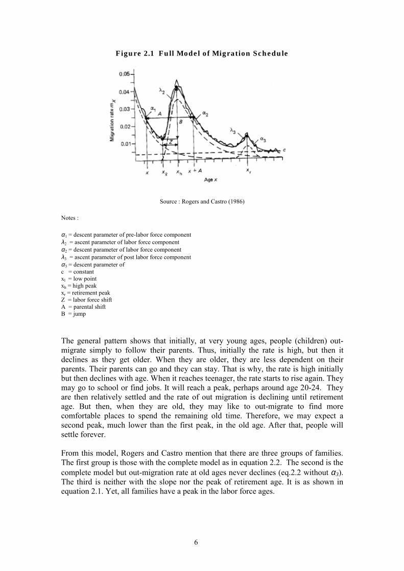
Figure 2.1 Full Model of Migration Schedule
Source : Rogers and Castro (1986)
Notes : α1 = descent parameter of pre-labor force component λ2 = ascent parameter of labor force component α2 = descent parameter of labor force component λ3 = ascent parameter of post labor force component α3 = descent parameter of c = constant xl = low point xh = high peak xr = retirement peak Z = labor force shift A = parental shift B = jump The general pattern shows that initially, at very young ages, people (children) out-migrate simply to follow their parents. Thus, initially the rate is high, but then it declines as they get older. When they are older, they are less dependent on their parents. Their parents can go and they can stay. That is why, the rate is high initially but then declines with age. When it reaches teenager, the rate starts to rise again. They may go to school or find jobs. It will reach a peak, perhaps around age 20-24. They are then relatively settled and the rate of out migration is declining until retirement age. But then, when they are old, they may like to out-migrate to find more comfortable places to spend the remaining old time. Therefore, we may expect a second peak, much lower than the first peak, in the old age. After that, people will settle forever. From this model, Rogers and Castro mention that there are three groups of families. The first group is those with the complete model as in equation 2.2. The second is the complete model but out-migration rate at old ages never declines (eq.2.2 without α3). The third is neither with the slope nor the peak of retirement age. It is as shown in equation 2.1. Yet, all families have a peak in the labor force ages.
7
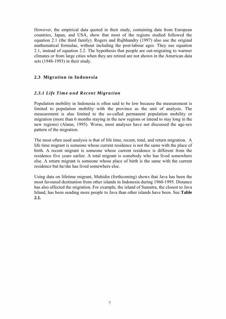
However, the empirical data quoted in their study, containing data from European countries, Japan, and USA, show that most of the regions studied followed the equation 2.1 (the third family). Rogers and Rajbhandry (1997) also use the original mathematical formulae, without including the post-labour ages. They use equation 2.1, instead of equation 2.2. The hypothesis that people are out-migrating to warmer climates or from large cities when they are retired are not shown in the American data sets (1948-1993) in their study. 2.3 Migration in Indonesia 2.3.1 Life Time and Recent Migration Population mobility in Indonesia is often said to be low because the measurement is limited to population mobility with the province as the unit of analysis. The measurement is also limited to the so-called permanent population mobility or migration (more than 6 months staying in the new regions or intend to stay long in the new regions) (Alatas, 1995). Worse, most analyses have not discussed the age-sex pattern of the migration. The most often used analysis is that of life time, recent, total, and return migration. A life time migrant is someone whose current residence is not the same with the place of birth. A recent migrant is someone whose current residence is different from the residence five years earlier. A total migrant is somebody who has lived somewhere else. A return migrant is someone whose place of birth is the same with the current residence but he/she has lived somewhere else. Using data on lifetime migrant, Muhidin (forthcoming) shows that Java has been the most favoured destination from other islands in Indonesia during 1960-1995. Distance has also affected the migration. For example, the island of Sumatra, the closest to Java Island, has been sending more people to Java than other islands have been. See Table 2.1.
8
Table 2.1 Distribution of Life Time Migration: Indonesia, 1971-1995
Place of Residence (at census or survey time) Place of birth Year Sumatra Java Kalimantan Sulawesi Other Islands
Alatas (1995) calculates that the percentage of lifetime migrant in the whole Indonesia has increased from 4.94% in 1971 to 8.25% in 1990. The percentage of total migrant has risen from 6.24% in 1971 to 9.95% in 1990; and the percentage of recent migrant has increased from 2.97% in 1971 to 3.32% in 1990. This pattern indicates the rising population mobility in Indonesia, even though the data is still limited to long term, population mobility and inter-provincial migration. Following Tirtosudarmo (1997), Muhidin explains that the rising volume of population mobility in Indonesia is due to three factors. First is the relative surplus of unskilled labor, fighting to get good jobs in the labor market. Second is the improvement in transportation and information networking. The labor market has been widening. The third is the booming of informal sector in the urban area. The informal sector has been an easy target for job seekers.
9
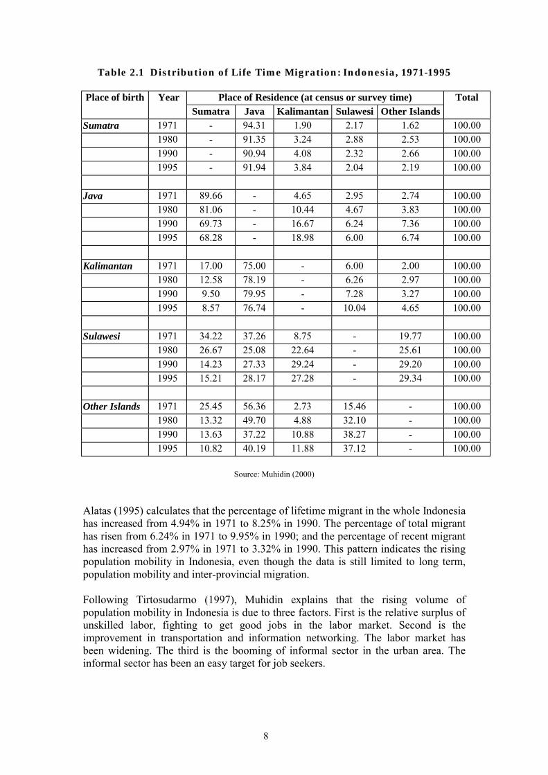
2.3.2 Age-Sex Pattern Ananta and Anwar (1995) have started to produce estimates of migration by age and sex for the 27 provinces in Indonesia. They estimate for periods of 1975-1980 and 1985-1990. They produce both age-sex specific in-migration and out-migration rates in each province. Yet, the in-migration rate is still calculated based on the population at destination, instead of the number of population at origin. They find that the pattern of out-migration for all provinces in both periods have the left-skewed unimodal curve, with the peak mostly at age 20-24. Very few are in 15-19 or 25-29. Male Bengkulu, South Sumatra, Central Sulawesi, West Nusa Tenggara, Irian Jaya and Maluku 1975-1980 and Male Jambi, Irian Jaya, male and female East Kalimantan 1985-1990 show the complete model (eq.2.2) without α3. Female Irian Jaya, male and female Southeast Sulawesi 1975-1980 and female Southeast Sulawesi 1985-1990 show the complete model. The old-age out-migration in the above provinces may be because they are the transmigrants who return to their homeland when they are old. The female may be married to the local and that may be why there is no increase in the female out-migration in the retirement ages. The remaining, the majority, shows the pattern without retirement ages (eq.2.1). Interestingly, they find a similar pattern for the in-migration. The pattern also has a left-skewed unimodal curve, with the peak around 20-24. As in out-migration, most pattern does not have a retirement age pattern, though some, but very few, have a rising in-migration during the retirement age. Jakarta in both periods and West Sumatra in 1975-1980 are two examples. The people in West Sumatra are famous for its merantau and so they may be those perantau who return home when they are old.1 The absence of such a pattern in 1985-1990 may indicate that they did not want to return to West Sumatra. Alternatively, the merantau had diminished because they did not have to merantau. West Sumatra had already been prospering and it was easy for people from West Sumatra to go everywhere without having to settle for a long time in the new regions. In terms of trend, Ananta and Anwar find seven groups. First group (West Sumatra, West Java, Central Java, East Java, Bali, South Sulawesi, West Nusa Tenggara, and Maluku) consists of eight provinces with rising in-migration and declining out-migration. Second group is those with declining of both out- and in-migration with five provinces: Jambi, Bengkulu, South Sumatra, North Sumatra, and Central Sulawesi. Third one consists of four provinces (with no change in migration rate), Aceh, North Sumatra, West Kalimantan, and Central Kalimantan. Fourth group, rising in both in- and out-migration: Yogyakarta, East Kalimantan, and Irian Jaya. The fifth is the provinces, which observed rising in out-migration and no change in in-migration, Southeast Sulawesi and East Nusa Tenggara. The sixth group is those with declining in-migration and rising out-migration: Jakarta and Lampung. The last, seventh group, experienced rising in-migration and no change in out-migration: Riau and South Kalimantan. They measure migration with Gross Migra Out Production Rate and Gross Migra In-Production Rate.2 See Table 2.2.
10
Table 2.3 Grouping of Trend of In-Migration and Out-Migration in Indonesian Provinces, 1975-1990
First Group: Rising In Migration and Declining Out Migration West Sumatra West Java Central Java East Java Bali South Sulawesi West Nusa Tenggara Maluku
Second Group : Declining in both In and Out Migration Jambi Bengkulu South Sumatra North Sumatra Central Sulawesi
Third Group : No Change in Migration Rate Aceh North Sumatra West Kalimantan Central Kalimantan
Fourth Group : Rising in both In and Out Migration Yogyakarta East Kalimantan Irian Jaya
Fifth Group : Rising Out Migration but no change in In Migration Southeast Sulawesi East Nusa Tenggara
Sixth Group : Declining In Migration and Rising Out Migration Jakarta Lampung
Seventh Group : Rising In Migration and no change in Out Migration Riau South Kalimantan
Source: Ananta and Anwar (1995)
Chotib (1998) estimates the age-sex pattern for out-migration and in-migration for Jakarta in 1990-1995. The in-migration is calculated as those lived in Jakarta in 1995 but lived outside Jakarta in 1990. The denominator is the number of population
11
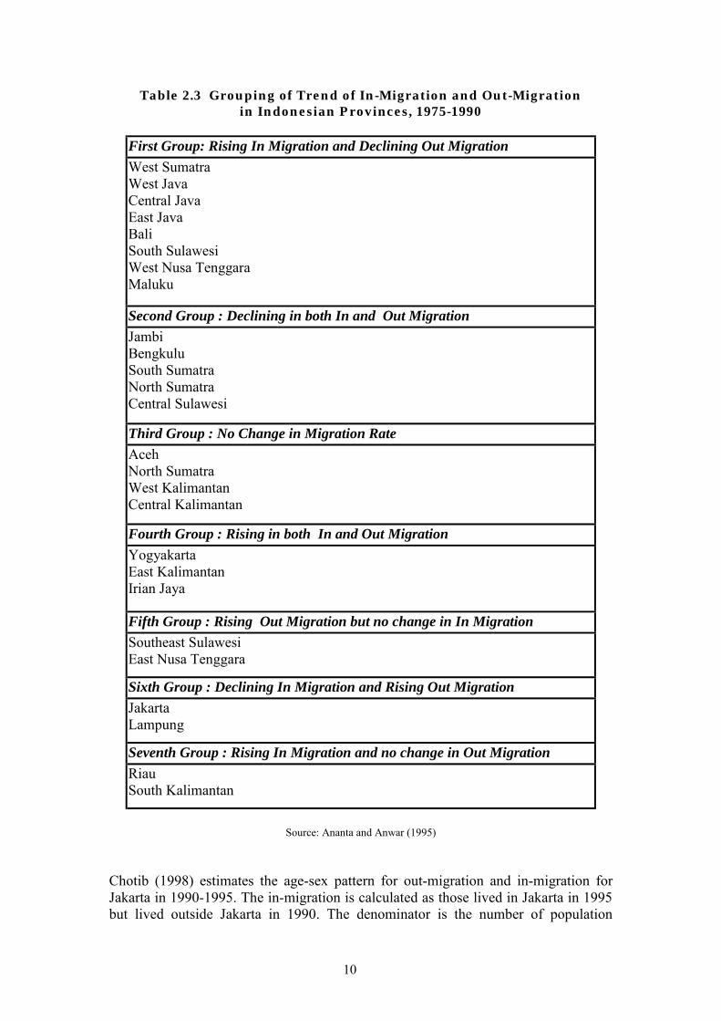
outside Jakarta in 1995 plus the migrants to the Jakarta in 1995. Actually, what he calculates is out-migration from "the rest of Indonesia". Therefore, we refer his estimate on "in-migration to Jakarta" as "out-migration from the rest of Indonesia". He works with individual age and uses a non-linear least square analysis to estimate equation 2.2. He then gets the estimated probability of out-migration from Jakarta and the rest of Indonesia. He groups the individual age group into five-year groups and represent his result in Figure 2.2.1 and Figure 2.2.2.
Figure 2.2.1 Age Pattern of Out-Migrants from Jakarta, 1990-1995
Figure 2.2.2 Age Pattern of Out-Migrants from the Remaining Indonesia, 1990-1995
Source : Chotib (1998) The sharp steep during age 50-65 for out-migration female in DKI is surprising. Does it mean that the female population has an earlier retirement period? The rate of out-migration from the rest of Indonesia is much lower than from Jakarta. This relatively much lower rate may be because the "remaining Indonesia" is simply too big compared to Jakarta, whose population is only about 4.7% of the total Indonesian population. It is also interesting that Chotib finds that rate of out-migration from Jakarta is greater for those born outside Jakarta and that out-migration from the rest of
Male
0
0.02
0.04
0.06
0.08
0.1
0.12
0.14
0.16
5-9
15-1
9
25-2
9
35-4
0
45-4
9
55-5
9
65-6
9
75-7
9
85+
Ag e
Rat
e
ASM R
Es t-ASM R
Female
0
0.02
0.040.06
0.08
0.1
0.120.14
0.16
5-9
15-1
9
25-2
9
35-4
0
45-4
9
55-5
9
65-6
9
75-7
9
85+
Ag e
Rat
e
ASM R
Es t-ASM R
Male
0
0.02
0.04
0.06
0.08
0.1
0.12
0.14
0.16
5-9
15-1
9
25-2
9
35-4
0
45-4
9
55-5
9
65-6
9
75-7
9
85+
Ag e
Rat
e
ASM R
Es t-ASM R
Female
0
0.02
0.04
0.06
0.08
0.1
0.12
0.14
0.16
5-9
15-1
9
25-2
9
35-4
0
45-4
9
55-5
9
65-6
9
75-7
9
85+
Ag e
Rat
e
ASM R
Es t-ASM R
12
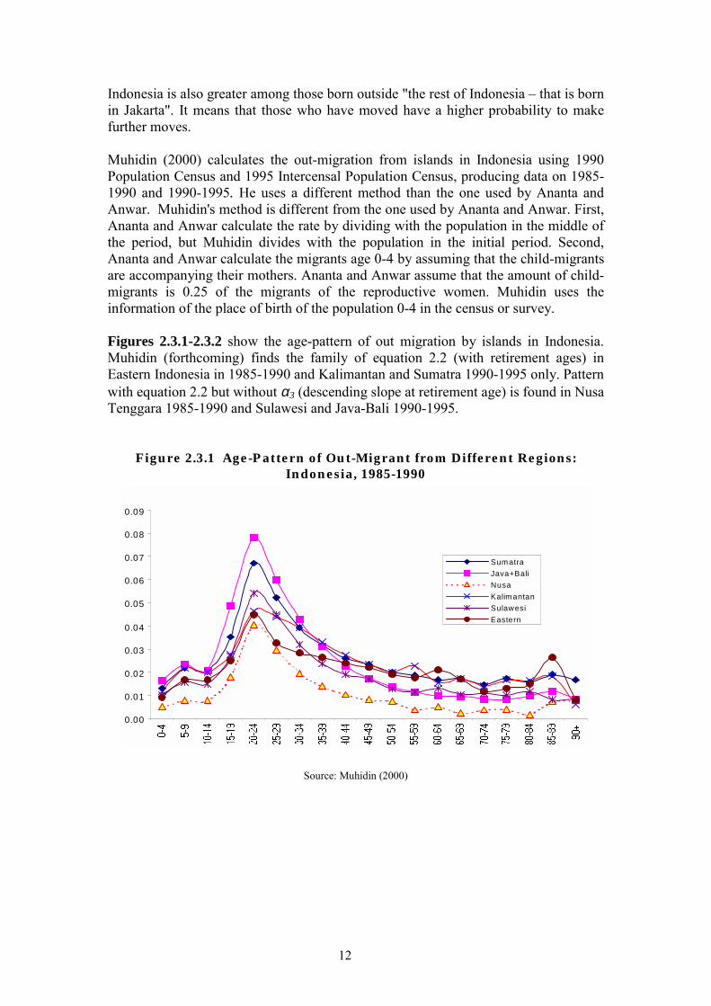
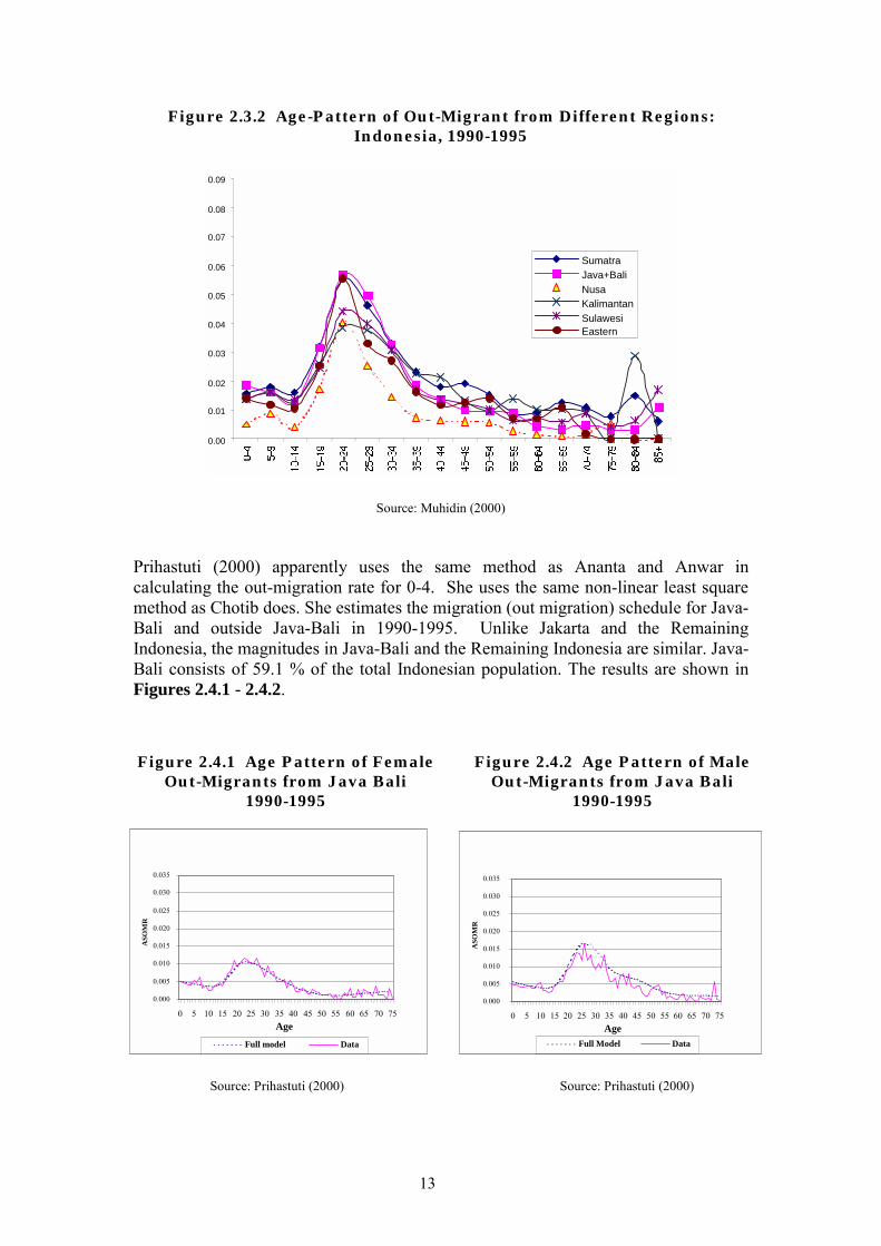
Indonesia is also greater among those born outside "the rest of Indonesia � that is born in Jakarta". It means that those who have moved have a higher probability to make further moves. Muhidin (2000) calculates the out-migration from islands in Indonesia using 1990 Population Census and 1995 Intercensal Population Census, producing data on 1985-1990 and 1990-1995. He uses a different method than the one used by Ananta and Anwar. Muhidin's method is different from the one used by Ananta and Anwar. First, Ananta and Anwar calculate the rate by dividing with the population in the middle of the period, but Muhidin divides with the population in the initial period. Second, Ananta and Anwar calculate the migrants age 0-4 by assuming that the child-migrants are accompanying their mothers. Ananta and Anwar assume that the amount of child-migrants is 0.25 of the migrants of the reproductive women. Muhidin uses the information of the place of birth of the population 0-4 in the census or survey. Figures 2.3.1-2.3.2 show the age-pattern of out migration by islands in Indonesia. Muhidin (forthcoming) finds the family of equation 2.2 (with retirement ages) in Eastern Indonesia in 1985-1990 and Kalimantan and Sumatra 1990-1995 only. Pattern with equation 2.2 but without α3 (descending slope at retirement age) is found in Nusa Tenggara 1985-1990 and Sulawesi and Java-Bali 1990-1995.
Figure 2.3.1 Age-Pattern of Out-Migrant from Different Regions: Indonesia, 1985-1990
0.00
0.01
0.02
0.03
0.04
0.05
0.06
0.07
0.08
0.09
SumatraJava+BaliNusaKalimantanSulawesiEastern
Source: Muhidin (2000)
Figure 2.3.2 Age-Pattern of Out-Migrant from Different Regions: Indonesia, 1990-1995
0.00
0.01
0.02
0.03
0.04
0.05
0.06
0.07
0.08
0.09
SumatraJava+BaliNusaKalimantanSulawesiEastern
Source: Muhidin (2000) Prihastuti (2000) apparently uses the same method as Ananta and Anwar in calculating the out-migration rate for 0-4. She uses the same non-linear least square method as Chotib does. She estimates the migration (out migration) schedule for Java-Bali and outside Java-Bali in 1990-1995. Unlike Jakarta and the Remaining Indonesia, the magnitudes in Java-Bali and the Remaining Indonesia are similar. Java-Bali consists of 59.1 % of the total Indonesian population. The results are shown in Figures 2.4.1 - 2.4.2.
Figure 2.4.1 Age Pattern of FemaleOut-Migrants from Java Bali
1990-1995
13
Source: Prihastuti (2000)
0.000 0.005 0.010 0.015 0.020 0.025 0.030 0.035
0 5 10 15 20 25 30 35 40 45 50 55 60 65 70 75 Age
ASO
MR
Full model Data
Figure 2.4.2 Age Pattern of Male Out-Migrants from Java Bali
2.4 Studies on Moving in Indonesia There is no quantitative data on moving, though moving is believed to have been much more common with the progress of economic development in Indonesia. Progress in economic development had brought better income (which is needed to move), better transportation, and better information. The relative flexibility of the labor market had also allowed for an increasing number of moving. Migration needs much bigger effort than moving and hence, it is not surprising that during crisis people may tend to move more than to migrate. Hugo (2000) concludes that during the recent crisis people had moved more than migrated to cope with the crisis. Hugo (1997) notes that, compared to the 1970s, women have participated more in both migration and moving. Yet, with the more formalization of the jobs, moving has also been more difficult. Women who work in factories in the urban areas, for example, have less flexibility to move between the rural and urban area. They then tended to migrate to the urban areas. However, at the same time, urbanization had also increased vary rapidly. This rapid urbanization had created more informal jobs, which in turn provided opportunities for more moving. They might work in the boundaries of the cities and they moved between the cities and their homes. In short, he asserts that, at least in Java, moving from rural areas to urban areas had increased very rapidly, more than the increase in migration from rural areas to urban areas. Quoting several small scale qualitative studies, Hugo (1997) has found that the increasing moving from Javanese villages had contributed to the increase in their economic welfare. He cites Collier et al in a longitudinal study in 37 villages in Java for the period of 1967-1991:
"Twenty years ago many of the landless labourers on Java had very few sources of income...Now most of the landless rural families on Java have at least one person who is working outside of the village, and in a factory or service job."
Figure 2.4.3 Age Pattern of Female Out-Migrants from the Remaining
Indonesia 1990-1995
Figure 2.4.4 Age Pattern of Male Out-Migrants from the Remaining
Indonesia 1990-1995
0.000 0.005 0.010 0.015 0.020 0.025 0.030 0.035
0 5 10 15 20 25 30 35 40 45 50 55 60 65 70 75 Age
ASO
MR
Full Model Data
0.000 0.005 0.010 0.015 0.020 0.025 0.030 0.035
0 5 10 15 20 25 30 35 40 45 50 55 60 65 70 75 Age
ASO
MR
Full Model Data
15
With the current trend toward regional autonomy, to be implemented in the year 2001, where the regions will have more authority to decide what they want to do, the difference in the pattern between moving and migration can be ambiguous. For example, if East Kalimantan province, which is rich with oil, gets a much higher share of its oil revenue and they can have more freedom to decide what they want, the province can lure people to come to East Kalimantan. Will people come to East Kalimantan to migrate, that is to stay there for a relatively long time, more than six months? Or, they will just circulate: they will come to East Kalimantan for three months, than return to their own province. Or, will the people in East Kalimantan themselves circulate more to exploit the rising opportunities in around the growth centers?
Unfortunately, there have not been any quantitative study comparing moving and migration, even at a small-scale study. This paper attempts to fill in the gap in this literature. The data set used is at a small scale, not representing the province in even Indonesia, but it incorporates information on both migrants and movers. With this data set, the paper attempts to compare the magnitude and pattern of migrants and movers by age and sex. The framework follows the one described by the first family of the previously described model of migration (equation 2.1). However, the data set does not have information on out-migration and even we cannot calculate the rate of out-migration. What it has is the migrants in the area. They came from other areas. Therefore, our result cannot be directly comparable to those based on data on rates of out-migration. Yet, our result is expected to contribute toward a better understanding on the comparison between migrants and movers. A better data set, which allows the calculation of out-migration and moving at district and provincial levels, is required. Unfortunately, the current 2000 Population Census still does not include questions on moving; it is still limited to migration.
16
Section 3 Data Set and Statistical Model 3.1 Source of Data
he data was collected by the Central Board of Statistics, Indonesia, funded by the United Nations Development Program in Jakarta and the National Development
Planning Board (Bappenas), in August 1998, one year after the crisis hit Indonesia. This is the first quantitative survey on population mobility which includes information on both �short term� and "non-permanent" population mobility. Other quantitative information is also asked through population censuses and intercensal population surveys, but they are limited to migration � the "long term" or "permanent" population mobility. The survey, which is called "Study Dampak Krisis terhadap Ketahanan Ekonomi Rumah Tangga: Migrasi" [Study on the Impact of the Crisis on Household Economic Resilience: Migration], is much smaller in scale compared to the intercensal surveys or even the population censuses. Yet, its advantage lies on its information about "non-permanent" or "short-term" population mobility along with one on the usual migration data. Therefore, this survey enables a comparison between these two types of population mobility. The survey also asks a set of socioeconomic information including the coping mechanism during the crisis The survey was conducted in seven provinces. From each province the survey selected one district (kabupaten). The districts covered were: North Lampung district (Lampung province), Indramayu district (West Java province), Wonogiri district (Central Java province), Bangkalan disrtrict (East Java province), Central Lombok district (West Nusa Tenggara province), Banjar district (South Kalimantan province), and Bone district (South Sulawesi province). The sample of the survey is households where at least one of the members was a "migrant" or a "mover". Three sub-districts were purposively selected from each district; two villages from each sub-district; and then two enumeration areas from each village. From the listing of households, 20 households were purposively selected in one enumeration area. An exception is in Banjar, where they had only 26 households in two selected villages. It should be noted that the choice of district, sub-district, village, and enumeration area is merely based on the recommendation of local key persons, either provincial/ district local statistical offices or heads of villages. They recommended according to what they believed as the areas with a tradition of out-migration. In other words, the sample can be biased for those areas where the respondents were likely to out-migrate.
Then, information was asked to all members of the households. The survey covers 7,738 individuals within 1,662 households in 42 villages, distributed almost equally in each of the seven provinces. The unit of analysis for defining a migrant, a mover, or a stayer is sub-district (kecamatan).
T
17
3.2 Migrants, Movers, and Stayers It is always difficult to define �migrant�. In Indonesian censuses and national surveys, a migrant is often defined as a �life time migrant�, a person whose place of current residence is different from his/her place of births. Or, a migrant is defined as a current migrant, a person whose current place of residence is different from his/her residence five years earlier. A person is said to stay in one residence if he/she has lived in that area for at least six months or that he/she intends to stay in that area. All definitions use province as the geographical unit.
In this study a migrant is defined as a current migrant, but different from the usual operational definition in the census and national surveys. Here, a (current) migrant is someone who either: a. has moved into the current residence (sub-district) between August 17, 1997 and
February 1998 (six months) before the survey or b. has moved into the current residence (sub-district) after February 1998 (6 months
before the survey) but he/she intends to stay in the current residence..
This definition of current migrant is more �current� than ones used in the census and national surveys. This definition should be maintained for future purposes, such as in SUPAS (Survey Penduduk Antar Sensus Intercensal Population Survey) and Population Censuses. It reflects more �current� phenomenon. The smaller geographical unit, the sub-district, is expected to be better able to capture population mobility. Further, the time period between August 17, 1997 and February 1998 is to catch the immediate impact of the crisis, which began by the end of July 1997, on migration. This survey also collected information on movers, the "non-permanent" or "short-term" population mobility. In this survey, a mover is defined as someone who either: a. has always been staying in the current residence (sub-district), but often going
outside the sub-district for at least one month. or b. has moved in before August 17, 1997 (that is, more or less, before the crisis
began) and often gone outside the sub-district for at least one month.
The remaining, the stayers, are those who are neither migrants nor movers. In the data used here, it is impossible to be both a migrant and a mover simultaneously, though, in reality, it is possible that he/she is a current migrant, who moved between 6 to 12 months earlier, and also a mover, who often goes outside the sub-district. Next survey should consider this one. 3.3 Description of Sampled Population In total there were 7,738 individuals. We then exclude 125 individuals who were out-migrants (who had not been members of the households since August 17, 1997.) We
18
also limit our study to population age 10-80. We exclude those age above 80 because they may be outlier or wrong information. We do not include those under 10 because we want to know the correlation of the probability with marital status and education.
With this limitation, there were 6,412 individuals, consisting of 3,995 (62.31%) stayers; 1,053 (16.42%) movers; and 1,364 (21.27%) migrants. As shown in Table 3.1, the movers, compared to the migrants and stayers, tend to consist more male and more rural. The migrants tend to be more urban, more educated, and more not married. The stayers tend to be more female and less educated. In other words, leaving the place of origin seems to require more "flexibility" (reflected in urban, more educated, and being not married).
Table 3.1 Some Characteristics of the Migrants, Movers, and Stayers
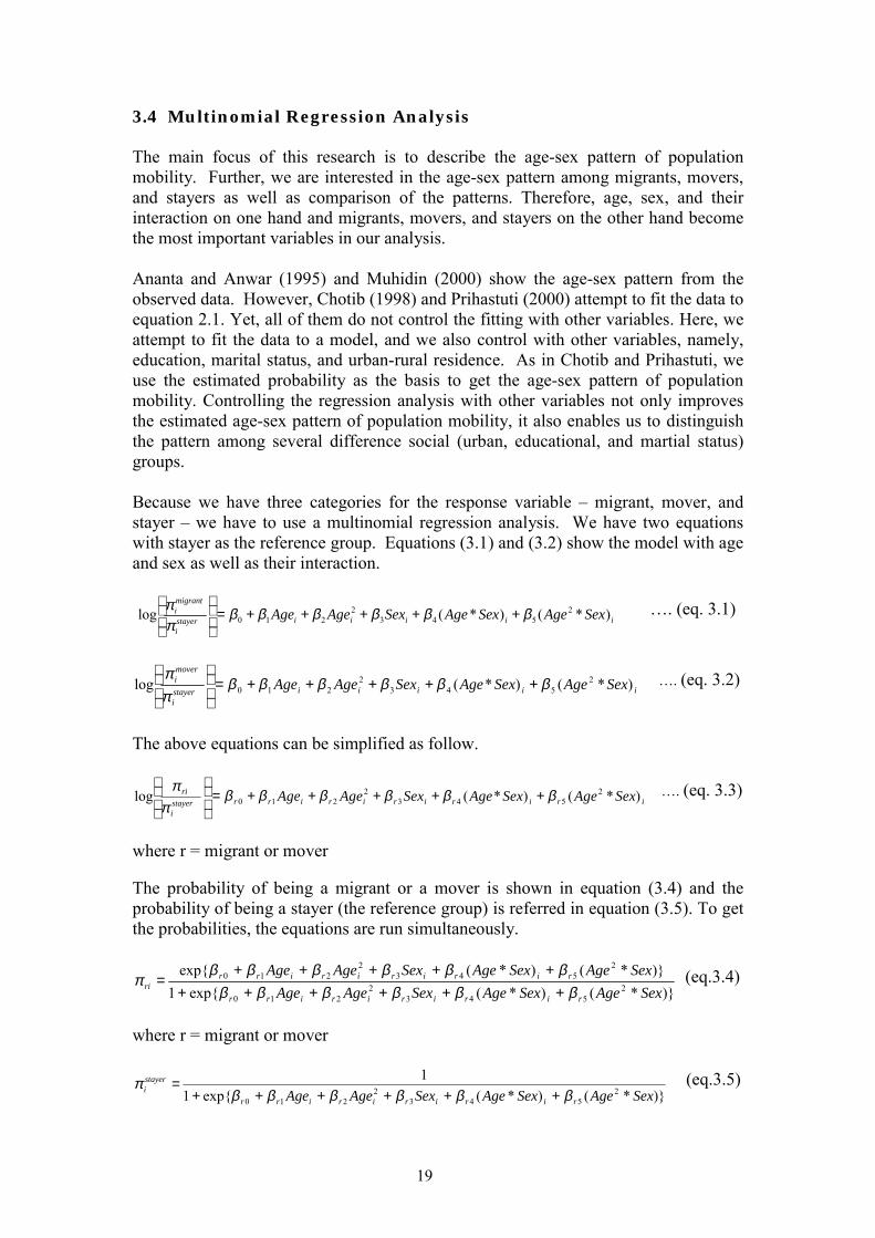
3.4 Multinomial Regression Analysis The main focus of this research is to describe the age-sex pattern of population mobility. Further, we are interested in the age-sex pattern among migrants, movers, and stayers as well as comparison of the patterns. Therefore, age, sex, and their interaction on one hand and migrants, movers, and stayers on the other hand become the most important variables in our analysis. Ananta and Anwar (1995) and Muhidin (2000) show the age-sex pattern from the observed data. However, Chotib (1998) and Prihastuti (2000) attempt to fit the data to equation 2.1. Yet, all of them do not control the fitting with other variables. Here, we attempt to fit the data to a model, and we also control with other variables, namely, education, marital status, and urban-rural residence. As in Chotib and Prihastuti, we use the estimated probability as the basis to get the age-sex pattern of population mobility. Controlling the regression analysis with other variables not only improves the estimated age-sex pattern of population mobility, it also enables us to distinguish the pattern among several difference social (urban, educational, and martial status) groups. Because we have three categories for the response variable � migrant, mover, and stayer � we have to use a multinomial regression analysis. We have two equations with stayer as the reference group. Equations (3.1) and (3.2) show the model with age and sex as well as their interaction.
iiiiistayer
i
migranti SexAgeSexAgeSexAgeAge )*()*(log 2
5432
210 ββββββππ +++++=
�. (eq. 3.1)
iiiiistayeri
moveri SexAgeSexAgeSexAgeAge )*()*(log 2
5432
210 ββββββππ
+++++=
�. (eq. 3.2)
The above equations can be simplified as follow.
iririririrrstayeri
ri SexAgeSexAgeSexAgeAge )*()*(log 2543
2210 ββββββ
ππ
+++++=
�. (eq. 3.3)
where r = migrant or mover The probability of being a migrant or a mover is shown in equation (3.4) and the probability of being a stayer (the reference group) is referred in equation (3.5). To get the probabilities, the equations are run simultaneously.
)}*()*(exp{1)}*()*(exp{
2543
2210
2543
2210
SexAgeSexAgeSexAgeAgeSexAgeSexAgeSexAgeAge
ririririrr
ririririrrri ββββββ
ββββββπ
+++++++++++
= (eq.3.4)
where r = migrant or mover
)}*()*(exp{11
2543
2210 SexAgeSexAgeSexAgeAge ririririrr
stayeri ββββββ
π++++++
= (eq.3.5)
20
We use a quadratic age function because we want to capture the labor force pattern with a peak.3 We do not estimate the post labor force pattern because previous studies show no significant post-labor force age pattern. We also exclude the pre labor force age pattern (under 10) because we want to investigate the relationship between the probability of migrant, mover, and stayer on one hand with educational status and marital status on the other hand. We incorporate all possible interactions between age and all other variables. Therefore in the model we also have the following variables: age, agesquare, sex, marital status, educ1, educ 2, urban, age*sex, agesquare*sex, age*marital status, agesquare*marital status, age*educ1, age*educ2, agesquare*educ1, agesquare*educ2, age*urban, agesquare*urban, K1, K2, K3, K4, K5, and K6. Marital status equals to 1 if married and 0 if unmarried. Sex equals to 1 if male and 0 otherwise, reference group is female. Educ1 is 1 if no schooling and 0 otherwise, and educ2 is 1 if primary school and 0 otherwise. Reference group is junior high school and above. Urban equals to 1 if urban and 0 otherwise. Rural is the reference group. Reference group for district (K) is Bone district, with K1 = 1 if Lampung Utara and 0 otherwise K2 = 1 if Indramaju and 0 otherwise K3 = 1 if Wonogiri and 0 otherwise K4 = 1 if Bangkalan and 0 otherwise K5 = 1 if Lombok Tengah and 0 otherwise K6 = 1 if Banjar and 0 otherwise We do not put interaction between the non age-sex variables because our attention is more on the age-sex pattern of population mobility. We also try models which control the age-sex pattern with some other explanatory variables, namely the urban-rural residence, education (no schooling, primary school, junior high school and above), marital status (married or not), and six dummy variables for the seven kabupatens (district). All variables refer to the time at the survey. 3.5 Multilevel Analysis Population mobility often occurs as a group. If one member of a household moves to one region, it is more likely that another member goes to the same place. In another words, we may have household clustering and region clustering. In our analysis, we have four levels of analysis. The first level is the individual. The second level, which is the first clustering, is the household. The third level (second clustering) is the enumeration area. The fourth level (third clustering) is sub-district (kecamatan) and the last level is district (kabupaten). Because there are only seven districts, we simply treat each district as a dummy variable. As shown by Goldstein (1999), statistical analysis which incorporates these clustering explicitly has the following advantages. First, the estimates of the regression coefficients are more efficient. Second, the results can be more "conservative" � those estimates which are insignificant without multilevel analysis can become significant once clustering is explicitly modeled in the analysis. Third, the multilevel analysis
21
enables the researchers to explore the contribution of clusters relative to the contribution of individual. In our research, multi level analysis will help us to learn whether clustering in migration affects probability of population mobility. Our multi-level analysis modifies equations 3.3.
rlrklrjklijklijklijklijklijkistayerijkl
rijkl swuSexAgeSexAgeSexAgeAge ++++++++=
)*()*(log 2
5432
210 ββββββππ (eq.3.3a)
where urjkl represents random effect in household level, wrkl represents random effect in enumeration area; and ssl is random effects in sub-district level. The three random effects are assumed to be mutually independent and normally distributed with mean zero and variances σrjkl
2, σrkl2 and σrl
2 respectively. The individual error term erijkl is assumed to follow a multinomial distribution.
where πrijkl represents the probability of being r for individual i in the jth household within kth enumeration area in lth sub-district. r can be either migrant or mover. And the probability of being a stayer is
})*()*(exp{11
2543
2210 ijklrijklrijklrijklrijkirr
stayerijkl SexAgeSexAgeSexAgeAge ββββββ
π++++++
= (eq.3.5a)
22
Section 4 Statistical Results 4.1 Impact of Age and Sex
able 4.1 shows the effect of age and sex without being controlled with other variables (education, marital status, and urban-rural residence). All coefficients
are significant, except for the impact of the interaction between agesquared and sex on probability of being a mover/ probability of a stayer. In other words, age and sex seem to have important effect on the probability of being a migrant, probability of being a mover, and probability of being a stayer. Further, the coefficients of the fixed parameters do not appear to be significantly different between those with unilevel model and those with multilevel model. Indeed, the data do not allow the examination of the variability of the fixed parameters across levels of analysis. The multilevel analysis conducted here focuses on the examination of the difference in the variation of the probability from one level to another.
Table 4.1 Impact of Age and Sex without Other Variables: Ordinary Model and Multilevel Model
Ordinary Model Multilevel Model
Migrant Mover Migrant Mover Parameter estimate of Variable
Notes: **** p < 0.001 *** p < 0.01 ** p < 0.05 * p < 0.1
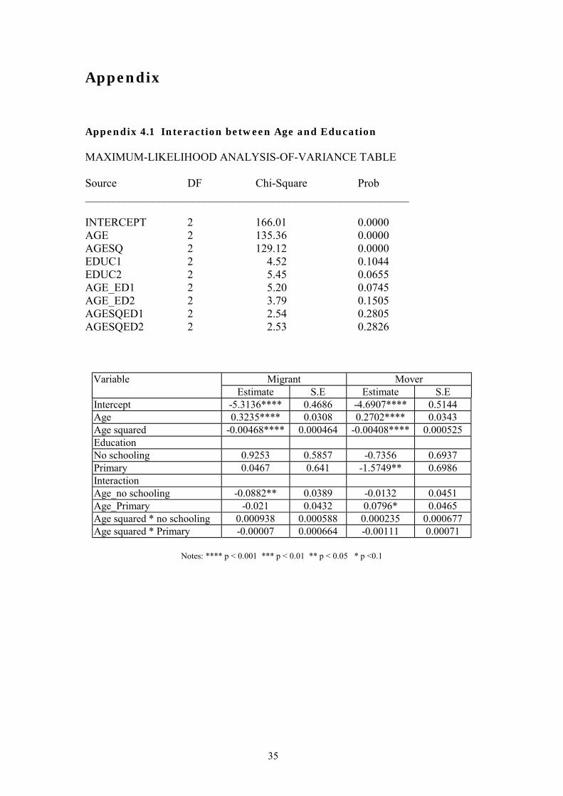
Table 4.2 shows the impact of age and sex on the ln (natural logarithm) of probability of being a migrant/probability of being a stayer and of probability of being a mover/ probability of being a stayer after being controlled by marital status, educational status, and urban-rural residence where the respondent stayed at the time of interview. We do not put interactions between age and education because we find serious multi-colinearity between age and interaction between age and education. Appendix 4.1 shows the result if we put the interaction between education and age.
T
23
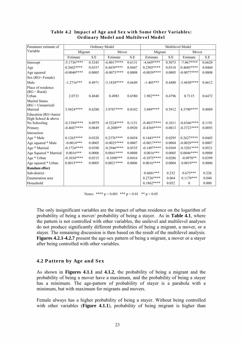
Table 4.2 Impact of Age and Sex with Some Other Variables: Ordinary Model and Multilevel Model
Ordinary Model Multilevel Model
Migrant Mover Migrant Mover Parameter estimate of Variable
Estimate S.E Estimate S.E Estimate S.E Estimate S.E Intercept -5.1736**** 0.5245 -6.8017**** 0.6131 -4.669**** 0.5073 -7.067**** 0.6628 Age 0.2602**** 0.0357 0.4439**** 0.0447 0.2505**** 0.0318 0.4605**** 0.0460 Age squared -0.0040**** 0.0005 -0.0073**** 0.0008 -0.0039**** 0.0005 -0.0077**** 0.0008 Sex (RG= Female) Male -1.2716*** 0.4971 -3.1838**** 0.6649 -1.405*** 0.4480 -3.4430**** 0.6612 Place of residence (RG = Rural)
Married 3.9424**** 0.6280 3.9787**** 0.8342 3.049**** 0.5912 4.3790**** 0.8089 Education (RG=Junior High School & above
No Schooling -0.3394**** 0.0979 -0.5224**** 0.1151 -0.4037**** 0.1011 -0.6366**** 0.1191 Primary -0.4687**** 0.0849 -0.2089** 0.0920 -0.4369**** 0.0813 -0.3723**** 0.0893 Interaction Age * Male 0.1265**** 0.0328 0.2376**** 0.0454 0.1443**** 0.0295 0.2627**** 0.0445 Age squared * Male -0.0014*** 0.0005 -0.0025**** 0.0007 -0.0017**** 0.0004 -0.0029**** 0.0007 Age * Married -0.1724**** 0.0398 -0.2946**** 0.0535 -0.1497**** 0.0369 -0.3201**** 0.0521 Age Squared * Married 0.0016*** 0.0006 0.0041**** 0.0008 0.0016*** 0.0005 0.0046**** 0.0008 Age * Urban -0.1034**** 0.0315 -0.1098*** 0.0416 -0.1075**** 0.0286 -0.0978** 0.0399 Age squared * Urban 0.0015**** 0.0005 0.0021**** 0.0006 0.0016**** 0.0004 0.0019*** 0.0006 Random effect Sub-district 0.6601*** 0.232 0.675*** 0.226 Enumeration area 0.2726**** 0.064 0.1179*** 0.040 Household 0.1862**** 0.052 0 0.000
Notes: **** p < 0.001 *** p < 0.01 ** p < 0.05
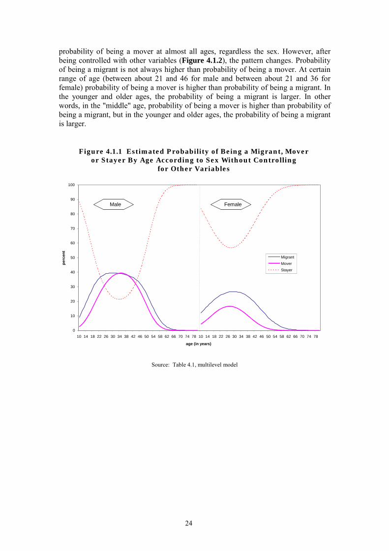
The only insignificant variables are the impact of urban residence on the logarithm of probability of being a mover/ probability of being a stayer. As in Table 4.1, where the pattern is not controlled with other variables, the unilevel and multilevel analyses do not produce significantly different probabilities of being a migrant, a mover, or a stayer. The remaining discussion is then based on the result of the multilevel analysis. Figures 4.2.1-4.2.7 present the age-sex pattern of being a migrant, a mover or a stayer after being controlled with other variables. 4.2 Pattern by Age and Sex As shown in Figures 4.1.1 and 4.1.2, the probability of being a migrant and the probability of being a mover have a maximum, and the probability of being a stayer has a minimum. The age-pattern of probability of stayer is a parabola with a minimum, but with maximum for migrants and movers. Female always has a higher probability of being a stayer. Without being controlled with other variables (Figure 4.1.1), probability of being migrant is higher than
probability of being a mover at almost all ages, regardless the sex. However, after being controlled with other variables (Figure 4.1.2), the pattern changes. Probability of being a migrant is not always higher than probability of being a mover. At certain range of age (between about 21 and 46 for male and between about 21 and 36 for female) probability of being a mover is higher than probability of being a migrant. In the younger and older ages, the probability of being a migrant is larger. In other words, in the "middle" age, probability of being a mover is higher than probability of being a migrant, but in the younger and older ages, the probability of being a migrant is larger.
0
10
20
30
40
50
60
70
80
90
100
perc
ent
Figure 4.1.1 Estimated Probability of Being a Migrant, Mover or Stayer By Age According to Sex Without Controlling
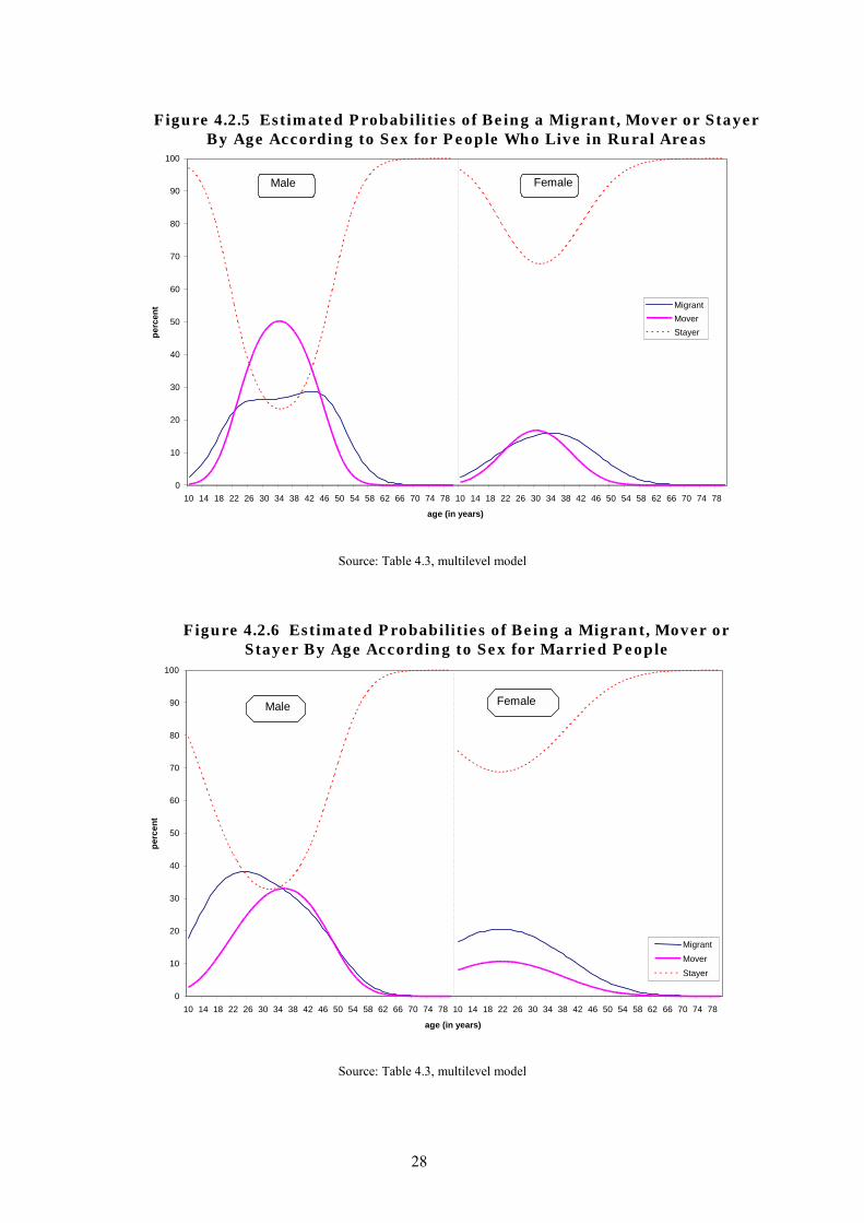
This pattern does not change when we differentiate by education, holding other variables at their mean values. See Figures 4.2.1 - 4.2.3. An exception is found only among female with no schooling, where probability of being a migrant is almost higher than probability of being a mover. The two probabilities coincide at about age 26-29. Figures 4.2.4 and 4.2.5 illustrate that the pattern neither changes after being controlled with urban-rural residence, with an exception for female in urban areas, where probability of being a migrant is always higher than probability of being a mover. The pattern of female in rural areas is almost similar to the pattern of female with no education. As shown in Figures 4.2.6 and 4.2.7, the pattern is still the same even after being controlled with marital status. Again, an exception is found among female respondents. Among married female, the probability of being a migrant is always higher than probability of being a mover.
Figure 4.2.6 Estimated Probabilities of Being a Migrant, Mover or Stayer By Age According to Sex for Married People
29
Source: Table 4.3, multilevel model
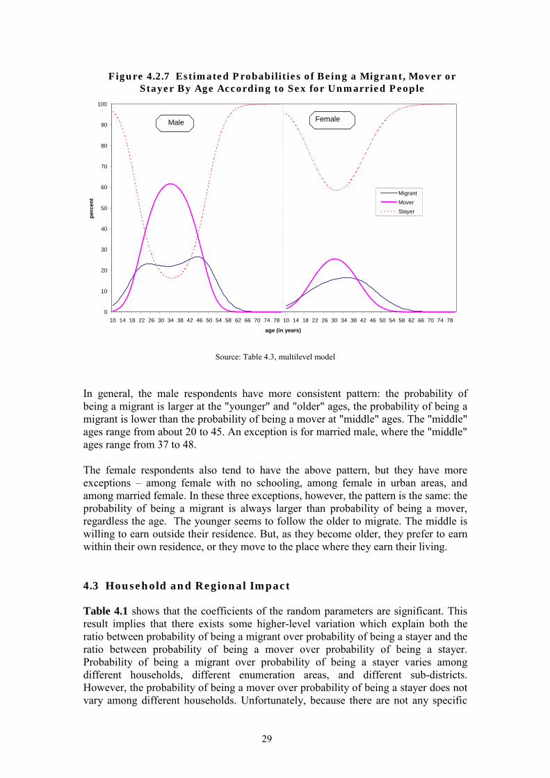
In general, the male respondents have more consistent pattern: the probability of being a migrant is larger at the "younger" and "older" ages, the probability of being a migrant is lower than the probability of being a mover at "middle" ages. The "middle" ages range from about 20 to 45. An exception is for married male, where the "middle" ages range from 37 to 48. The female respondents also tend to have the above pattern, but they have more exceptions � among female with no schooling, among female in urban areas, and among married female. In these three exceptions, however, the pattern is the same: the probability of being a migrant is always larger than probability of being a mover, regardless the age. The younger seems to follow the older to migrate. The middle is willing to earn outside their residence. But, as they become older, they prefer to earn within their own residence, or they move to the place where they earn their living. 4.3 Household and Regional Impact Table 4.1 shows that the coefficients of the random parameters are significant. This result implies that there exists some higher-level variation which explain both the ratio between probability of being a migrant over probability of being a stayer and the ratio between probability of being a mover over probability of being a stayer. Probability of being a migrant over probability of being a stayer varies among different households, different enumeration areas, and different sub-districts. However, the probability of being a mover over probability of being a stayer does not vary among different households. Unfortunately, because there are not any specific
Figure 4.2.7 Estimated Probabilities of Being a Migrant, Mover or Stayer By Age According to Sex for Unmarried People
30
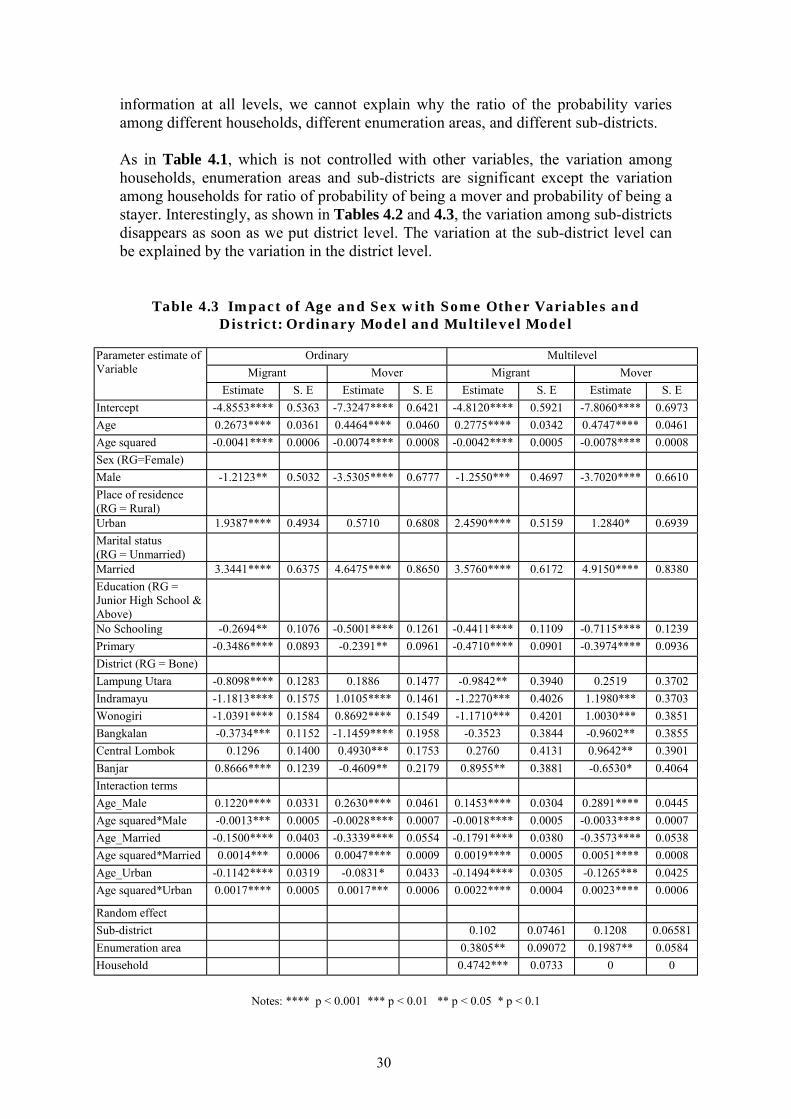
information at all levels, we cannot explain why the ratio of the probability varies among different households, different enumeration areas, and different sub-districts. As in Table 4.1, which is not controlled with other variables, the variation among households, enumeration areas and sub-districts are significant except the variation among households for ratio of probability of being a mover and probability of being a stayer. Interestingly, as shown in Tables 4.2 and 4.3, the variation among sub-districts disappears as soon as we put district level. The variation at the sub-district level can be explained by the variation in the district level.
Table 4.3 Impact of Age and Sex with Some Other Variables and District: Ordinary Model and Multilevel Model
Ordinary Multilevel
Migrant Mover Migrant Mover Parameter estimate of Variable
Estimate S. E Estimate S. E Estimate S. E Estimate S. E Intercept -4.8553**** 0.5363 -7.3247**** 0.6421 -4.8120**** 0.5921 -7.8060**** 0.6973 Age 0.2673**** 0.0361 0.4464**** 0.0460 0.2775**** 0.0342 0.4747**** 0.0461 Age squared -0.0041**** 0.0006 -0.0074**** 0.0008 -0.0042**** 0.0005 -0.0078**** 0.0008 Sex (RG=Female) Male -1.2123** 0.5032 -3.5305**** 0.6777 -1.2550*** 0.4697 -3.7020**** 0.6610 Place of residence (RG = Rural)
Random effect Sub-district 0.102 0.07461 0.1208 0.06581 Enumeration area 0.3805** 0.09072 0.1987** 0.0584 Household 0.4742*** 0.0733 0 0
Notes: **** p < 0.001 *** p < 0.01 ** p < 0.05 * p < 0.1
31
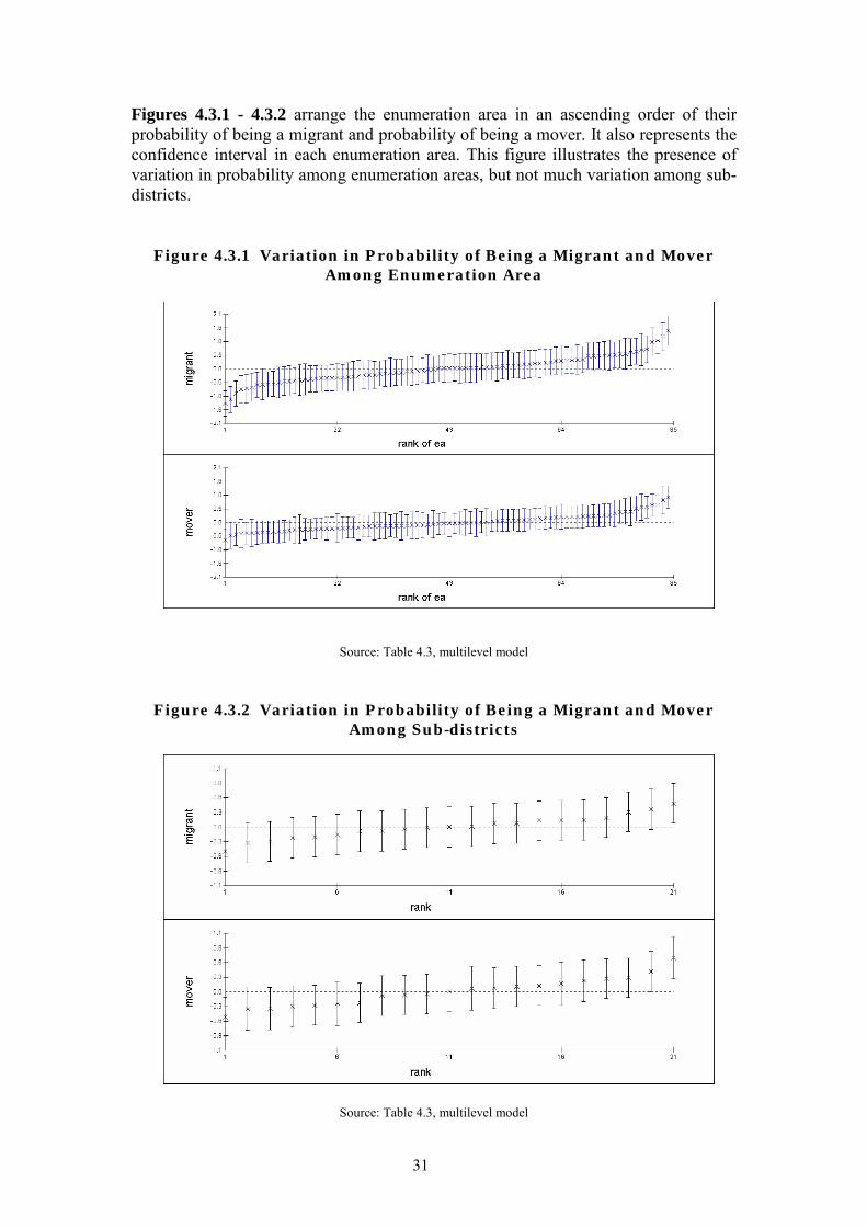
Figures 4.3.1 - 4.3.2 arrange the enumeration area in an ascending order of their probability of being a migrant and probability of being a mover. It also represents the confidence interval in each enumeration area. This figure illustrates the presence of variation in probability among enumeration areas, but not much variation among sub-districts.
Figure 4.3.1 Variation in Probability of Being a Migrant and Mover Among Enumeration Area
Source: Table 4.3, multilevel model
Figure 4.3.2 Variation in Probability of Being a Migrant and Mover Among Sub-districts
Source: Table 4.3, multilevel model
32
Therefore, the hypothesis of the impact of "chain networking" in being a migrant is not to reject at household level, enumeration area level, and district level. Some common "pull factors" at household, enumeration area, and district levels may have operated to pull people to in-migrate. However, the clustering for being a mover is only found at enumeration area and districts level. There may be some common "push factors", at enumeration and district levels, that drive people to earn outside their residence. Yet, there have not been any information on what variables at household, enumeration area, or district level which have contributed to the explanation of being a migrant, a mover, or a stayer.
33
Section 5 Conclusion
his study has contributed to the knowledge on the difference between the quantitative pattern of migrants and movers. In general, being a migrant has a
higher probability than being a mover at younger and older ages. In between, probability of being a mover is higher than probability of being a migrant. However, the ages at which they are called as younger or older vary depending on the characteristics of the respondents. "Older" can start as early as 34 as in the case of female respondents; and "younger" can last as late as 35 as shown in the case of male married respondents. In general, the "middle ages" range from 20 to 45. During the "middle ages" people are still willing to earn their living outside their residences. As they become older, they prefer to work within their own residence. The "younger" may follow the older and therefore the probability of being a migrant is higher than probability of being a mover for the "younger". There are some exceptions to this general pattern. Among female population with no schooling, probability of being a migrant is almost always higher than probability of being a mover. At around age 27, the probabilities are almost the same. Another exception is found among female population who live in urban area and among female married respondents. In this case, the probability of being a migrant is always higher than probability of being a mover. Yet, they have the same pattern: the probability of being a migrant is at least as high as the probability of being a mover. This study also shows that pattern of population mobility (either as migrant or as mover) can be different if the pattern is controlled with some other variables. Without being controlled with other variables, but only controlled by age and sex, probability of being a migrant is at least as high as the probability of being a mover. Though some studies have shown that age-sex pattern of out-migrants is similar to the age-sex pattern of in-migrants, the pattern produced in this study cannot be directly compared with the age-pattern of migration discussed in Section 2. The information collected in this study deals with in-migrants, instead of out-migrants. In addition, with the focus on in-migrants, this study can compare the probability of being a migrant, being a mover, and being a stayer. Among female, whatever the characteristics of the female respondents, the probability of being a stayer is always higher than probability of being a migrant and probability of being a mover. Among male, the probability of being a stayer is initially higher than probability of being a migrant and a mover, but at a certain point, the probability of being a stayer is lower than probability of being a mover and/ or a mover. At some later ages, the probability of being a stayer is again higher than probability of being a migrant or a mover. Further, the use of multilevel statistical analysis has enabled the study to conclude not to reject the hypothesis of the existence of "chain effect" in population mobility. Some common "pull factors" may have pushed people to earn their living outside their residence. Yet, further studies, with better data sets, should be carried out to explain
T
34
what kind of variables at household, enumeration area, and district which may explain the variation in probability of being a migrant and a mover.
Intercept -5.3136**** 0.4686 -4.6907**** 0.5144 Age 0.3235**** 0.0308 0.2702**** 0.0343 Age squared -0.00468**** 0.000464 -0.00408**** 0.000525 Education No schooling 0.9253 0.5857 -0.7356 0.6937 Primary 0.0467 0.641 -1.5749** 0.6986 Interaction Age_no schooling -0.0882** 0.0389 -0.0132 0.0451 Age_Primary -0.021 0.0432 0.0796* 0.0465 Age squared * no schooling 0.000938 0.000588 0.000235 0.000677 Age squared * Primary -0.00007 0.000664 -0.00111 0.00071
Notes: **** p < 0.001 *** p < 0.01 ** p < 0.05 * p <0.1
36
Bibliography Alatas, Secha. 1995. �Studi Migrasi Penduduk Indonesia� [A Study on Indonesian Population Migration] in Migrasi & Distribusi Penduduk di Indonesia [Migration and Population Distribution in Indonesia] edited by Secha Alatas. Jakarta: State Ministry of Population/ National Family Planning Coordinating Board. Ananta, Aris. 1995. "Transisi Mobilitas Penduduk Indonesia" [Transition of Indonesian Population Mobility] in Transisi Demografi, Transisi Pendidikan, dan Transisi Kesehatan di Indonesia [Demographic Transition, Education Transition and Health Transition in Indonesia] edited by Aris Ananta. Jakarta: State Ministry of Population/National Family Planning Coordinating Board. Ananta, Aris and Anwar, Evi Nurvidya. 1995. �Perubahan Pola dan Besaran Migrasi Propinsi: Indonesia, 1975-1980 dan 1985-1990� [Changes in Pattern and Magnitude of Provincial Migration: Indonesia, 1975-1980 and 1985-1990] in Migrasi & Distribusi Penduduk di Indonesia [Migration and Population Distribution in Indonesia] edited by Secha Alatas. Jakarta: State Ministry of Population/National Family Planning Coordinating Board. Central Bureau of Statistics (Indonesia); State Ministry of Population/National Family Planning Coordinating Board; Ministry of Health; and Macro International Inc. 1998. Indonesia Demographic and Health Survey 1997. Calverton, Maryland: CBS and MI. Chotib. 1998. "Skedul Model Migrasi dari DKI Jakarta/Luar DKI Jakarta: Analisis Data Supas 1995 dengan Pendekatan Demografi Multiregional" [Migration Model Schedule for Jakarta and outside Jakarta: An Analysis on 1995 Supas Data with Multiregional Demographic approach]. Thesis submitted for Master Degree in Population and Labor Study Program, Graduate Program, University of Indonesia. Coale, Ansley J. and Demeny, Paul. 1983. Regional Model Life Tables and Stable Populations. 2nd edition . New York : Academic Press. Collier, W.L.; Santoso, K.; Soentoro; and Wibowo, R. "New Approach to Rural Development in Java". mimeo as quoted in Hugo (1997). Goldstein, H. 1995. Multilevel Statistical Model. London: Edward Arnold and New York: Wiley. Hugo, Graeme. 1997. "Changing Patterns and Processes in Population Mobility" in Indonesia Assessment. Population and Human Resources. Edited by Gavin W. Jones and Terence H. Hull. Singapore: Institute of Southeast Asian Studies. Hugo, Graeme. 2000. "The Impact of the Crisis on Internal Population Movement in Indonesia" Bulletin of Indonesian Economic Studies, vol.36, no.2, August. Muhidin, S. Salut. 2000. "Regional Dimension of Migration by Education and Employment: The Case of Indonesia", paper presented at the International Conference "Immigration Societies and Modern Education". Singapore: Center for Advanced Studies, National University of Singapore, August 31 - September 3. Muhidin, S. Salut. forthcoming. Future Demographic of Indonesian Population. Multiregional Population Projection Using Various Data Sources. Ph.D dissertation, University of Groningen. Prihastuti, Dewi. 2000. "Model Pertumbuhan Penduduk Lanjut Usia (Lansia) di Indonesia Dengan Pendekatan Multiregional" [Growth Model for Aging Population in Indonesia with Multiregional Approach]Thesis submitted for Master Degree in Population and Labor, Graduate Program, University of Indonesia.
37
Rogers, Andrei. 1995. Multiregional Demography: Principles, Methods, and Extensions. Chichester: John Wiley. Rogers, Andrei and Castro, Luis J. 1986. "Migration" in Migration and Settlement. A Multiregional Comparative Study. Edited by Andrei Rogers and Frans J. Willekens, pp.157-210. Dordrecht, Holland: D. Reidel Publishing Company Rogers, Andrei and Rajbhandary, Sameer. 1997. "Period and Cohort Age Pattern of US Migration, 1948-1993: Are American Males Migrating Less?" Population Research and Policy Review 16:513-530. Rogers, Andrei; Raquillet, R; and Castro, L. J. 1978. "Model Migration Schedules and Their Applications" Environment and Planning A 10: 475-502. Tirtosudarmo, Riwanto. 1997. �Economic Development, Migration, and Ethnic Conflict in Indonesia: a preliminary observation� SOUJURN, Social Issues in Southeast Asia, Vol. 12, No.2.
38
Notes 1 Merantau can be roughly explained as the tradition of venturing outside the home region to earn money. Perantau is the person who merantau. 2 Gross Migra Production Rate is the summation of age specific migration rate. It is similar to Gross Fertility Rate in fertility analysis and it uses only out-migration. ( Rogers, 1995) However, Ananta and Anwar (1995) also calculate in-migration rate. Thus, they have Gross out Migra Production Rate and gross in Migra Production Rate. The trend in their analysis is based on these measurements. 3 Age is measured at single year.