26
AGGREGATE PLANNING (from Course Production Analysis) Advanced Production Planning Models 1
| Date post: | 19-Dec-2015 |
| Category: |
Documents |
| View: | 227 times |
| Download: | 0 times |
1
AGGREGATE PLANNING(from Course Production Analysis)
Advanced Production Planning Models

2
Extensions
• multiple products• different resource capacities
• backorders
• overtime
• subcontracting• capacities in different production areas
• alternative routing
3
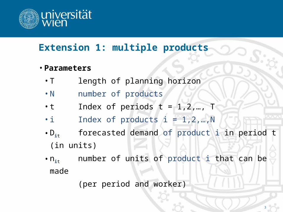
Extension 1: multiple products
• Parameters
• T length of planning horizon
• N number of products
• t Index of periods t = 1,2,…, T
• i Index of products i = 1,2,…,N
• Dit forecasted demand of product i in period t (in
units)
• nit number of units of product i that can be made
(per period and worker)

4
Extension 1: multiple products
• Parameters (cont)
• CitP costs to produce one unit of product i in t
• CtW cost of one worker in period t
• CtH cost of hiring one worker in t
• CtL costs to lay one worker off in t
• CitI inventory holding costs in t
(per unit of product i and period)
• CitB backorder costs in t
(per unit of product i and period)

5
Extension 1: multiple products
• Pit number of units of product i produced in period t
• Wt number of workers available in period t
• Ht number of workers hired in period t
• Lt number of workers laid off in period t
• Iit number of units of product i held in inventory at
end of period t
• Bit number of units of product i backordered at end
of period t
6
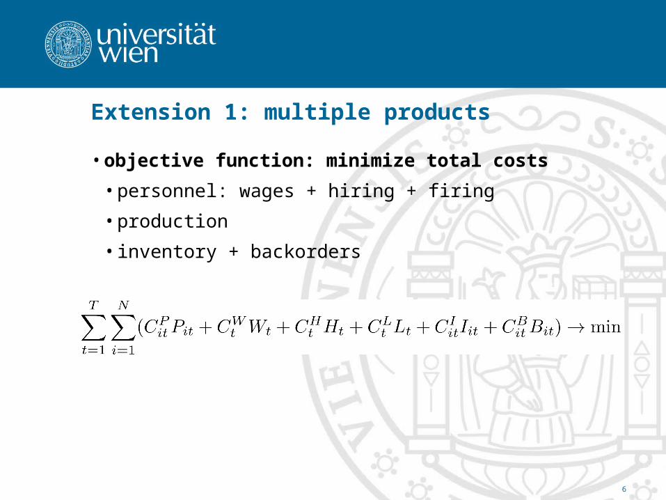
Extension 1: multiple products
• objective function: minimize total costs
• personnel: wages + hiring + firing
• production
• inventory + backorders

7
Extension 1: multiple products
• constraints
• capacity
• inventory balance
• workforce balance
• non-negativity
8
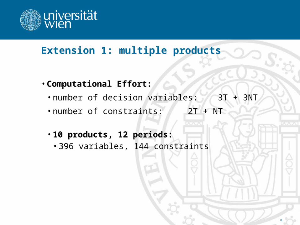
Extension 1: multiple products
• Computational Effort:
• number of decision variables: 3T + 3NT
• number of constraints: 2T + NT
• 10 products, 12 periods: • 396 variables, 144 constraints
9
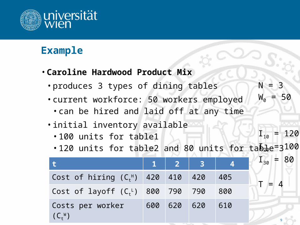
Example
• Caroline Hardwood Product Mix
• produces 3 types of dining tables
• current workforce: 50 workers employed • can be hired and laid off at any time
• initial inventory available• 100 units for table1• 120 units for table2 and 80 units for table 3
N = 3
W0 = 50
I10 = 120
I20 = 100
I30 = 80
T = 4
t 1 2 3 4
Cost of hiring (CtH) 420 410 420 405
Cost of layoff (CtL) 800 790 790 800
Costs per worker (CtW) 600 620 620 610
10
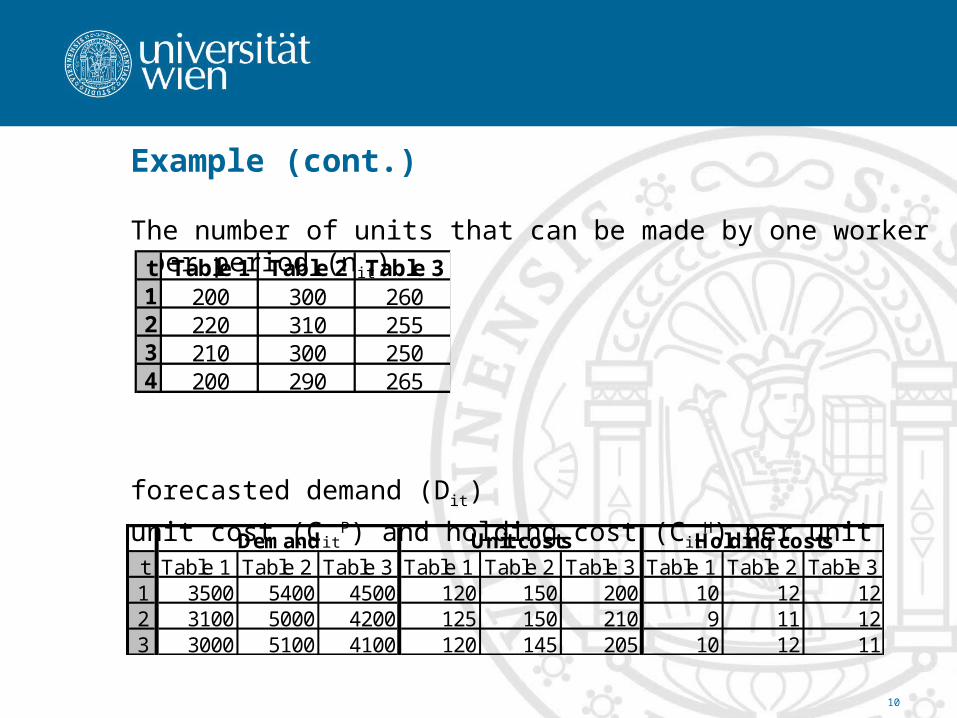
Example (cont.)
The number of units that can be made by one worker per period (nit)
forecasted demand (Dit)
unit cost (CitP) and holding cost (Cit
H) per unit
t Table 1 Table 2 Table 31 200 300 2602 220 310 2553 210 300 2504 200 290 265
t Table 1 Table 2 Table 3 Table 1 Table 2 Table 3 Table 1 Table 2 Table 31 3500 5400 4500 120 150 200 10 12 122 3100 5000 4200 125 150 210 9 11 123 3000 5100 4100 120 145 205 10 12 11
Demand Unit costs Holding costs
11
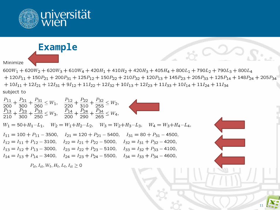
Example

12
Example
• Solution: total costs $ 8354165.72 Workers 1 2 3 4Hired (Ht) 1.60 0.00 0.00 5.64Laid Off (Lt) 0.00 3.91 0.00 0.00Workers (Wt) 51.60 47.69 47.69 53.32
Production (Pit) 1 2 3 4Table 1 (i=1) 3400.00 3100.00 3000.00 3400.00Table 2 (i=2) 5280.00 5000.00 5100.00 5500.00Table 3 (i=3) 4420.00 4200.00 4100.00 4600.00
Inventory (Iit) 1 2 3 4Table 1 (i=1) 0.00 0.00 0.00 0.00Table 2 (i=2) 0.00 0.00 0.00 0.00Table 3 (i=3) 0.00 0.00 0.00 0.00
13
Extension 2: Multiple Processes
• multiple products
• each of which may be manufactured in a different way
• different processes (with zero setup times)• possibly at different locations
• mi ways to produce product i
• different resources• workers, machines, departement• making one unit of product i using process j
requires aijk units of resource k

14
Extension 2: Multiple Processes
• Parameters
• T length of planning horizon
• N number of products
• K number of resource types
• t Index of periods t = 1,2,…, T
• i Index of products i = 1,2,…,N
• k Index of resource types k = 1,…,K
• mi number of different processes available for
making i

15
Extension 2: Multiple Processes
• Parameters (cont.)
• Dit forecasted demand of product i in period t (in
units)
• Akt amount of resource k available in period t
• aijk amount of resource k required to produce one
unit of product i if produced by process j
• CitP costs to produce one unit of product i in t
• CitI inventory holding costs in t
(per unit of product i and period)
16
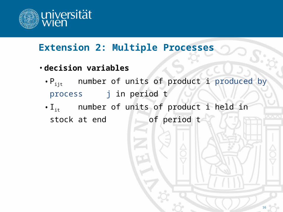
Extension 2: Multiple Processes
• decision variables
• Pijt number of units of product i produced by
process j in period t
• Iit number of units of product i held in stock at
end of period t
17
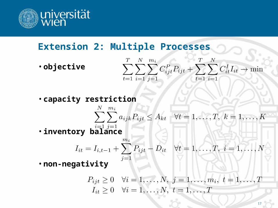
Extension 2: Multiple Processes
• objective
• capacity restriction
• inventory balance
• non-negativity
18
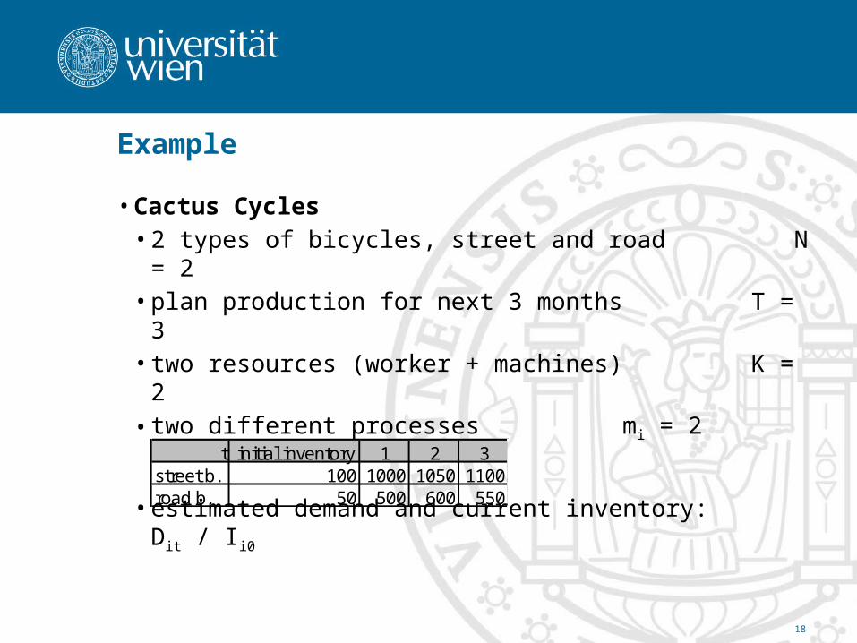
Example
• Cactus Cycles• 2 types of bicycles, street and road N = 2• plan production for next 3 months T = 3• two resources (worker + machines) K = 2
• two different processes mi = 2
• estimated demand and current inventory: Dit / Ii0 t initial inventory 1 2 3street b. 100 1000 1050 1100road b. 50 500 600 550

19
Example (cont.)
• available capacity Akt (hours) and holding costs per bike Iit
• process costs (Pijt) and resource requirement (aijk) per unit
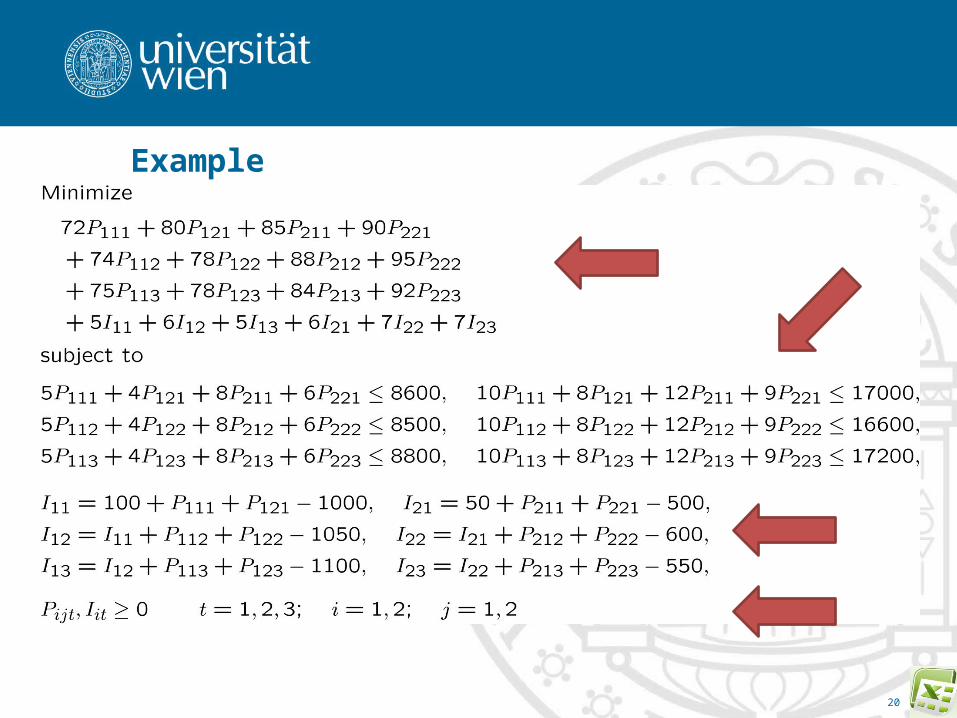
t Machine Worker Street Road1 8600 17000 5 62 8500 16600 6 73 8800 17200 5 7
Capacity(hours) Holding
t Street Road Street Road1 72 85 80 902 74 88 78 953 75 84 78 92
Machine hours required 5 8 4 6Worker hours required 10 12 8 9
Process1 Process2
20
Example

21
Example
• Solution
• objective (min costs) $ 368756.25
Produce (Pi1t) Produce (Pi2t)
1 2 3 1 2 3
Street (i=1) 900.00 1050.00 0.00 0.00 0.00 1100.00
Road (i=2) 118.75 406.25 550.00 525.00 0.00 0.00
Inventory (Iit) 1 2 3
Street (i=1) 0.00 0.00 0.00
Road (i=2) 193.75 0.00 0.00
22
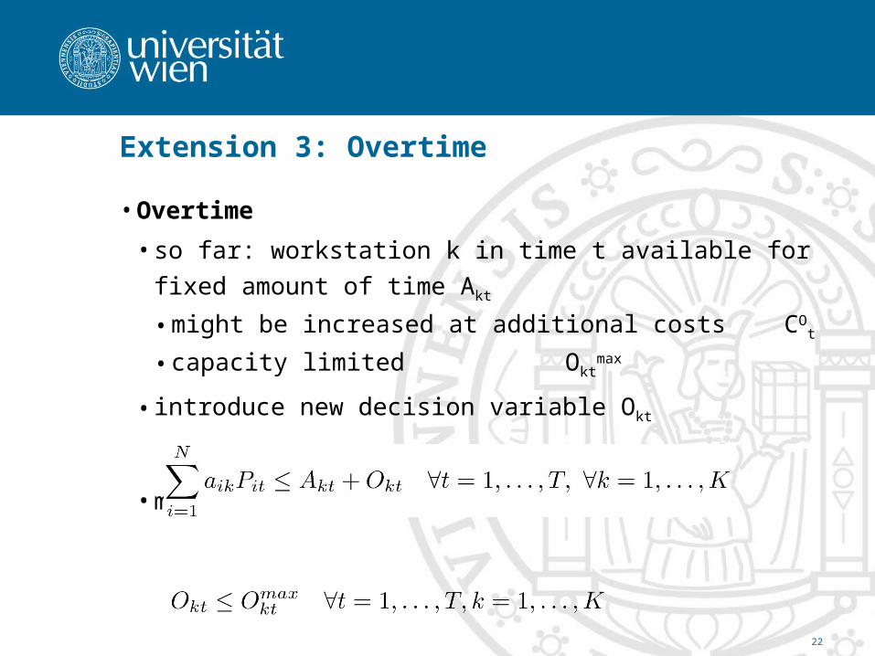
Extension 3: Overtime
• Overtime
• so far: workstation k in time t available for fixed amount of time Akt
• might be increased at additional costs COt
• capacity limited Oktmax
• introduce new decision variable Okt
• modify capacity restriction
• limit its availability

23
Extension 4: Yield Loss
• Yield Loss
• products may be scrapped at various points in the production
line (quality problems)
• release additional material to compensate for loss
• upstream workstations more heavily utilized
24
Extension 4: Yield Loss
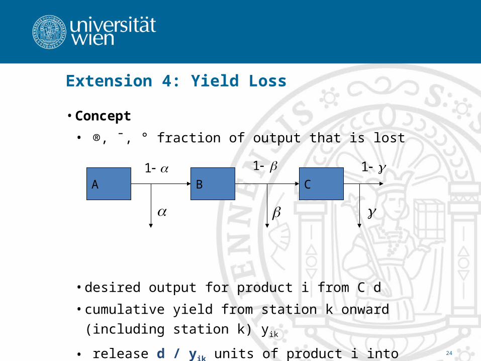
• Concept
• ®, ¯, ° fraction of output that is lost
• desired output for product i from C d
• cumulative yield from station k onward (including station k) yik
• release d / yik units of product i into station k
A B C1 1
1
25
Extension 4: Yield Loss
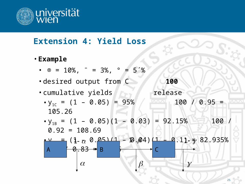
• Example
• ® = 10%, ¯ = 3%, ° = 5´%
• desired output from C 100
• cumulative yields release
• y1C = (1 – 0.05) = 95% 100 / 0.95 = 105.26
• y1B = (1 – 0.05)(1 – 0.03) = 92.15% 100 / 0.92 = 108.69
• y1A = (1 – 0.05)(1 – 0.04)(1 – 0.1) = 82.935% 100 / 0.83 = 120.5
A B C1 1
1

26
Extension 4: Yield Loss
• LP Formulation


![[PPT]Production and Operations Management: …sureten/(aggregate planning)5.ppt · Web viewDisaggregating the Aggregate Plan Aggregate Planning Aggregate planning Intermediate-range](https://static.documents.pub/doc/80x56/5aec86827f8b9ab24d902697/pptproduction-and-operations-management-suretenaggregate-planning5pptweb.jpg)


