Page 1
Agricultural and Rural Finance Markets in Transition
Proceedings of Regional Research Committee NC-1014
St. Louis, Missouri
October 4-5, 2007
Dr. Michael A. Gunderson, Editor
January 2008
Food and Resource Economics
University of Florida
PO Box 110240
Gainesville, Illinois 32611-0240
Page 2
1
Commodity Linked Credit:
A Risk Management Instrument for the Agrarians in India
Prepared by
Apurba Shee
Pennsylvania State University
Calum Turvey
Cornell University
Page 3
2
Abstract
This research analyzes daily commodity spot prices and designs risk contingent
structured financial instruments as a means to mitigate business and financial risk by
reducing debt obligations depending on the embedded commodity options whose payoffs
are linked with commodity price fluctuations. Models are developed for operating loans and
farm mortgages. The results show that the distributions with the embedded option have
higher probability of greater returns and the embedded option with the repayment
contingent on the price fluctuation reduces the downside risk of the return from the
investment.
Page 4
3
Introduction
The problem of endemic poverty in the agriculture of developing countries is largely
attributed to low-return economies of scale with any opportunity for increasing either the
scale or size of farm operations constrained by access to credit. On the matter of scale the
inability of farmers to access short run operating credit to purchase inputs limits the value of
total product that can be achieved. On the matter of size the inability to acquire longer term
credit, i.e. a mortgage, constrains farms to seemingly perpetual state of low output
livelihoods; a poverty trap. The two reasons that commercial lenders or rural cooperatives
are so reserved in their lending to developing agriculture is because these farmers have in
limited resources insufficient collateral to support the loan, and second, even if collateral
were sufficient, because the business risks arising from adverse price and weather
movements is so high relative to scale, that the likelihood of default is almost
insurmountable.
The question then is what can be done to resolve this problem in a practical way?
This paper offers a very novel and practical solution in the form of commodity-linked credit.
Commodity-linked credit are structured financial products that have imbedded options
against price movements. We present two formulations in this paper each designed to deal
with different problems. On the operating side we evaluate a standard single period
operating loan with repayment tied to the price of an underlying commodity. The built-in
price protection reduces downside risk to the farmer and simultaneously the risk of default
to the lender and this unto itself would increase the supply of credit to agriculture. To
manage growth and increase economies of size we evaluate a commodity-linked mortgage.
This product offers contingent credit in each year of the mortgage; that is in any year that
commodity prices fall below a stated target the principal payment required in that year is
reduced. It is important not to confuse these products with schemes that merely postpone
Page 5
4
payment in times of adversity. The products discussed in this paper remove entirely from
present or future liability the indemnified risk. The removal of risk of course comes at a cost,
and in this paper the formulas presented solve for the risk adjusted interest rate for the
operating and mortgage products.
The formulas we present are unique. Turvey (2007) developed the formulas for
weather-linked credit and indeed in agricultural economies that face greater peril from
weather risk than price risk the formulas can be as easily applied. We also believe that the
formulas can be used in developing micro-loans. Micro-finance institutions have in many
regions entered into group-lending activities that provide entrepreneurial and consumption
capital. Group lending activity to farmers however is constrained by the commonality of risk
across its members; that is if all members are involved in the same or highly correlated
production activities then any price fall will impact all of the group members at once. The
operating loan discussed in this paper resolves this problem because the commodity linkage
will protect all group members equally.
The region we address in this paper is particularly well suited for the type of product
we propose. Indian agriculture faces wide commodity price fluctuation which makes the
return from investment vulnerable and risks the debt repayment ability of farmers. When
farmers face adverse market prices, they frequently receive less revenue and when that
occurs they often can not repay the debt they took for the investment. The accumulation of
unpaid loans limits their access to new capital, which in turn makes their investment in
agriculture vulnerable. To meet their financial obligations farmers are forced to sell fixed
assets such as land, trees, jewelries etc. leading to an abysmally poverty trap from which few
escape. Sometimes the situation becomes so unbearable that farmers in large numbers
commit suicide (Mohanty (2005), Mishra (2007), Jeromi (2007)).
Page 6
5
There is also a political will in India that makes our credit products attractive.
Government intervention offers some relief with subsidized credit (e.g SGSY ;Swarnajayanti
Gram Swarozgar Yojana) with the intent of increasing credit access; however, the subsidized
SGSY loan is limited to farmers Below Poverty Line (BPL) leaving with limited or no access a
large percentage of the population. To encourage commercial lending the government has
been promoting community organization around small saving and credit groups49 and banks
then provide loans to the groups considering the groups as social collateral. This aids lenders
in the mitigating information imperfections (adverse selection and moral hazard) 50
(Armendariz and Morduch 2005) but group lending unto itself does not hedge against price
risks, especially if all group members are involved in growing the same commodity or
commodities that are highly correlated in price. Despite the group lending and peer pressure
for the repayment, the business risk (price-fluctuation) can lead to default by the entire
group. Consequently, group lending amongst poor farmers is not that common in Indian
agriculture and because of the inherent business risks individual lending is heavily rationed.
As discussed earlier, commodity-linked credit can be plied by MicroFinance Institutions (MFI)
to micro loans of farmer-centric self help groups as well as to individual farmers with only
limited access to collateral.
The overall objective of this study is to investigate the applicability of price contingent
credit as a means of balancing business and financial risks for pulse crops in India. We
49
A Self Help Group is an informal and socio-economically homogeneous association of 10 to 20
persons, who meet weekly for the business of savings and credit for enhancing the financial security
and raising the economic status of its members. It acts not only as a microfinance intermediary but also
a platform for sustainable livelihood and women empowerment. 50
Adverse selection is the lenders inability to assess which borrower is risky and which one is safe.
Moral hazard problem in lending is referred to as banker‘s inability to observe the effort taken or the
realization of the return by the borrower.
Page 7
6
investigate three types of commodity dominated structured financial products- operating
loans, farm mortgages and commodity bonds. The specific objectives are:
i. To investigate historical pattern of price movements for pulses in India. In order to
accomplish this objective, we calculate annual volatilities of pulse cash price series in
some Indian local wholesale markets.
ii. To determine the range of interest rates that could be charged to risk contingent
credit for pulses. To accomplish this goal, we construct model structures of
contingent claims such that the repayments of the credit instruments are contingent
on the pulse market price variable in India.
iii. To test the effectiveness of commodity credits on the livelihood of a typical
household in Sunderpahari, a block in eastern India. To investigate this, we generate
the distributions of the portfolio return of the household by simulation.
Commodity-Linked Credit
In this section we present the basic model for commodity linked credit. The
principles involved follow from Turvey (2006) who explores a range of commodity-linked
bond structures and Turvey (2008) who develops the formulas used here in an application to
weather-linked credit. Most medium and small farmers require operating loans for a crop
year (around 8 months to 1 year). Farmers take money for the investment on the crop
production and generally repay the loan amount by selling their produce after the harvest.
Price variation of the commodities directly affects their repayment ability to the banks. The
repayment risk can be hedged by structuring the repayment of the operating loan with
commodity price fluctuation. The lenders portfolio of an initial operating loan of f amount
with embedded commodity option can be written as,
Page 8
7
(1) ))]](,0[max([*
tSKfeeB TrrT
where r is the discount rate, K is strike price, *r is the interest rate charged on the operating
loan which reflect the lender’s cost of capital, and K
f. Now, the present value of the
operating loan without the commodity can be written as,
(2) TrrT feeB )(
1
**
Therefore, to hedge the price risk with the embedded commodity option, the interest rate
charged by the lender ( *r ) can be calculated by equating (1) and (2);
(3) TrrTTrrT feetSKEfee )( ***
))]](,0[max([ ,
and solving for *r ;
(4) T
ef
tSKE
r
Tr )(
*
**))](,0[max(ln
Equation (4) provides the exact formula for calculating the interest rate on an operating loan
with payment protection against low commodity prices.
To see how equation (4) works, we determine the interest rate for a non-revolving
operating loan for Ranchi bengalgram a pulse crop. From calculations that will be described
presently, the price for Ranchi bengalgram has a natural Brownian drift of 11.6% and
annualized volatility of 31.5%. Assuming a risk-free discount rate of 5%, a one year at-the-
Page 9
8
money put option premium priced with a general equilibrium formula with the current cash
price of Rs. 2,825 is Rs. 215.43 assuming the market price of risk is 0. Assuming a base
interest rate of 12% for conventional loans and an operating loan of Rs.20,000 then
08.72825
000,20
K
f, and from equation (4) the interest rate on the operating loan
(5) 1854.0000,20
43.21508.7ln 12.* er .
Hence, the risk adjusted interest rate is 18.54% or a risk premium of 6.54% above the
price of a loan without the contingencies. If the cash price of Ranchi bengalgram falls below
the strike, Rs. 2,825, the loan repayment obligation also falls. For example, if the commodity
price at termination falls to Rs.2542.5, then the payout on the option part is
2000)0,5.25422825(08.7 Max , and the loan amount repaid after 1 year
0.185420,000 2,000 22,075e Rupees. In comparison the loan without the embedded
option would be .1220,000 22,550e Rupees. What this boils down to is that producers
get a protection against the downside price risk. Figure 1 shows the decreasing loan
repayment obligation as the prices decrease. The loan repayment without the option is
depicted by the horizontal line.
Page 10
9
Figure 3.1: Commodity price and the loan obligations with options
Farm mortgage
A farm mortgage is one of the established ways for a farm owner to get a loan from a
financial institution. In this case the farmer has to keep the farm as collateral for the
borrowed money with the provision that if the loan is not repaid the lender has the right to
the borrower’s farm. Mathematically an annuity formula for a T year mortgage of the total
loan amount F can be written as;
(6)
1
)1(1)(
i
iFiA
T
,
where )(iA is the amortization of the lump-sum amount F into T smaller cash flows. Now
applyingK
iA )(, the value of the mortgage with an embedded commodity option is as
follows;
Commodity price vs loan obligation
0
5000
10000
15000
20000
25000
30000
0 500 1000 1500 2000 2500 3000 3500 4000
Ranchi Bengalgram prices
Lo
an
rep
aym
en
t
Page 11
10
(7) r
etSKE
K
iAe
r
iAB
rTrT )1(
))](,0[max()(
)1()( *
If r is the discount rate applied to the present value of the amortization without any option
then the value of the mortgage to the lender is:
(8) )1()(
1
rTer
iAB
Now to completely hedge the amortization repayment against commodity output price risk,
the mortgage rate ( *i ) can be calculated by equating (7) and (8) to obtain
(9)
1
*
* ))](,0[max(1
)1(1)1(1
K
tSKE
i
i
i
i TT
,
which can be solved using an iterative process.
Suppose a farmer wants to raise Rs (INR) 150,000 for investment in bengalgram
cultivation by mortgaging the property for ten years. The amortization for Rs. 150,000 of 10-
year mortgage at 12% base interest rate is Rs. 26,547.62 per year. The embedded a-the-
money option as calculated previously is 215.43. Solving equation (9) we get i * =14% which is
2% higher than the base interest rate of 12% and when applied to the farm mortgage, yields
an amortization of Rs.28,572.04 per year. If we suppose in a particular time the price of
Ranchi Bengalgram is 2,542.5, then the repayment in that year would be
26,547.6228,572.04 [max(2,825 2,542.5),0]
2,825 or Rs. 25,917.28 which is less than the
base amortization value. Figure 2 depicts the decreasing amortization payments with the fall
Page 12
11
in commodity prices where horizontal line represent the amortization payment without the
option51.
Figure 5.1: Commodity prices with bond repayment
Background area and local wholesale market price data
The study focuses on a block called Sundarpahari in the Godda district of Eastern
India, which is home to indigenous Santhal and Paharia tribes. The Santhals live in the plain
51 An alternative which we do not present in this paper is a commodity-linked bond. with the
entire periodic cash flow requirement for coupon payment and sinking fund;
r
etSKMaxE
K
T
Fc
Feer
cB
rTrTrT 1
))](,0([)1( ,
where the bond yield rate r =discount rate.
Commodity prices vs bond repayment
0.00
50000.00
100000.00
150000.00
200000.00
250000.00
300000.00
0 500 1000 1500 2000 2500 3000 3500
Prices
Rep
aym
en
t
Page 13
12
area and cultivate rice, maize and different types of pulses such as Bengalgram (Cicer
aritinum L.), Masur(Lentil), field pea, lathyrus (khesari) and rajmas during rabi season and
Arhar( Cajanus cajan), Greengram (Vigna radiate), horse gram, Cowpea (Vigna unguiculata)
during kharif52 season. The paharias reside on the hilltops and practice shifting cultivation on
the slopes and produce Cowpeas, Arhar, maize, and pearl millets.
The motivation for examining different pulses crop in this paper is that farmers who
produce pulses in significant portions require credit for pulse cultivation. In the absence of
access to commercial lending most of the Santhal and Paharia family borrow money from the
local moneylenders. In the months of July and August people take loans ranging from Rs 500
to Rs 10,000 for the labor intensive pulses cultivation53. These loans are in the form of seeds,
rice and cash from local money lenders. The loans are normally repaid by December-January
and the interest charged by moneylenders is 50 to 100%. However, it is often the case that
low harvest prices lead to loan default. In this process of indebtedness, many families resort
to distress sale of fixed assets huge live trees of Mango, Jackfruit, Mahua etc. at low prices.
Many families lose their land to the money lenders. The lack of formal lending has been a
major impediment to economic growth in the region. Despite efforts through government
and non government initiatives to develop formal lending activities, lender concerns about
price variation still constrain capital.
Volatility in Pulse Crop Prices
Commodity price data was downloaded from the Agricultural Marketing Information
System Network (AGMARKNET) (http://www.agmarknet.nic.in), a central sector scheme of
52
There are two major cropping seasons in India, namely, Kharif and Rabi. The Kharif season is during
the south-west monsoon (July-October). During this season, agricultural activities take place both in
rain-fed areas and irrigated areas. The Rabi season is during the winter months, when agricultural
activities take place only in the irrigated areas. 53
This is based on survey data collected by senior author in 2003-2004 during in Sundarpahari
Page 14
13
Directorate of Marketing and Inspection (DMI), Department of Agriculture & Cooperation,
Ministry of Agriculture, India and compiled into a historical time series of daily commodity
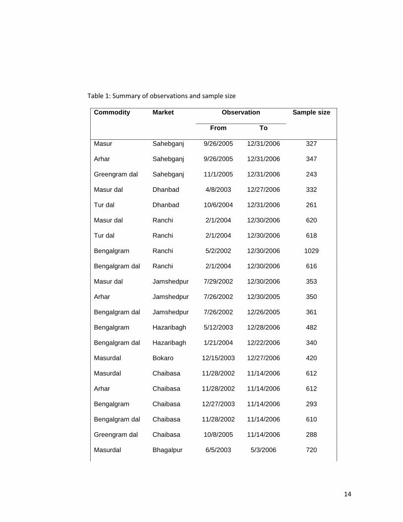
cash prices. Summary of observations and sample sizes of daily modal cash prices of pulse (a
leguminous commercial crop) commodities namely Masurdal, Arhar, Greengram dal, Turdal,
Bengalgram, Bengalgram dal, and Cowpea are provided in Table 1 with their respective local
wholesale markets. The Cowpea does not have a local wholesale market, more generally
selling in the south and west Indian markets. Therefore, the study analyzes some wholesale
markets for Cowpea like Koppal and Gadag in Karnataka, Jhunjhunu in Rajastan, and Lalitpur
in UP. Prices in these markets can influence the return of the farmers of the outlined area.
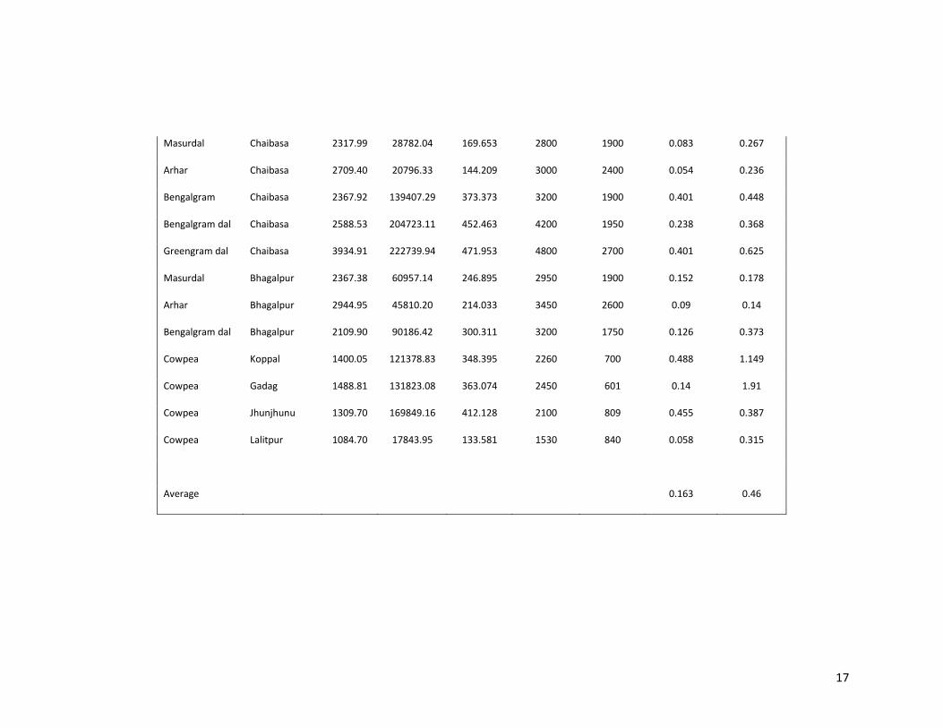
The data are summarized Table 2. Prices are represented by Rs (INR) per quintal (100 kg).
Prices have high variances (standard deviations) within the period, the highest standard
deviation being 641.5 for Ranchi Bengalgram dal, 520.2 for Sahebgang Greengram dal, and
472 for Chaibasa Greengram dal. The data show that except for Sahebganj Masur and Ranchi
Masur, all commodities in the respective markets enjoy annual price gains over the study
period with the average annual gain being 16.3%. The largest annual price increases are
Koppal Cowpea, Jhunjhunu Cowpea, Hazaribagh Bengalgram dal, and Chaibasa Greengram
dal at 48.8%, 45.5%, 43% and 40.1% respectively. Sahebganj Masur and Ranchi Masur show
the annual price decline of 1.6% and 4.7% respectively. The most volatile pulse is Gadag
Cowpea at 191% followed by Koppal Cowpea at 114.9%, Hazaribagh Bengalgram at 75.4%,
Chaibasa Greengram dal at 62.5% and Hazaribagh Bengalgram dal at 58.2%. Volatility of 14%
for Bhagalpur Arhar is the least volatile while Bhagalpur Masurdal has the second lowest
volatility of 17.8%. On an average the annual volatility of all the combination is 46%.
Page 15
14
Table 1: Summary of observations and sample size
Commodity Market Observation Sample size
From To
Masur Sahebganj 9/26/2005 12/31/2006 327
Arhar Sahebganj 9/26/2005 12/31/2006 347
Greengram dal Sahebganj 11/1/2005 12/31/2006 243
Masur dal Dhanbad 4/8/2003 12/27/2006 332
Tur dal Dhanbad 10/6/2004 12/31/2006 261
Masur dal Ranchi 2/1/2004 12/30/2006 620
Tur dal Ranchi 2/1/2004 12/30/2006 618
Bengalgram Ranchi 5/2/2002 12/30/2006 1029
Bengalgram dal Ranchi 2/1/2004 12/30/2006 616
Masur dal Jamshedpur 7/29/2002 12/30/2006 353
Arhar Jamshedpur 7/26/2002 12/30/2005 350
Bengalgram dal Jamshedpur 7/26/2002 12/26/2005 361
Bengalgram Hazaribagh 5/12/2003 12/28/2006 482
Bengalgram dal Hazaribagh 1/21/2004 12/22/2006 340
Masurdal Bokaro 12/15/2003 12/27/2006 420
Masurdal Chaibasa 11/28/2002 11/14/2006 612
Arhar Chaibasa 11/28/2002 11/14/2006 612
Bengalgram Chaibasa 12/27/2003 11/14/2006 293
Bengalgram dal Chaibasa 11/28/2002 11/14/2006 610
Greengram dal Chaibasa 10/8/2005 11/14/2006 288
Masurdal Bhagalpur 6/5/2003 5/3/2006 720
Page 16
15
Arhar Bhagalpur 6/5/2003 5/3/2006 758
Bengalgram dal Bhagalpur 6/5/2003 5/3/2006 705
Cowpea Koppal 5/2/2003 12/28/2006 278
Cowpea Gadag 5/2/2002 12/18/2006 639
Cowpea Jhunjhunu 10/11/2003 12/30/2006 438
Cowpea Lalitpur 12/20/2002 12/30/2006 525
Page 17
16
Table 2: Sample statistics of commodity market prices, annualized geometric growth rates and volatilities
Commodity Market Mean Variance
Standard
deviation Maximum Minimum
Annual
Geometric
mean
Annualize
volatility
Masur Sahebganj 2478.13 45487.00 213.277 2850 2050 -0.016 0.243
Arhar Sahebganj 3041.90 55345.22 235.256 3500 2400 0.0202 0.389
Greengram dal Sahebganj 3959.47 270571.20 520.165 4800 3050 0.383 0.5108
Masur dal Dhanbad 2475.66 25151.44 158.592 2800 2025 0.118 0.393
Tur dal Dhanbad 2984.70 28293.08 168.205 3250 2550 0.032 0.395
Masur dal Ranchi 2331.18 16002.00 126.499 2700 2000 -0.047 0.228
Tur dal Ranchi 2801.87 21244.30 145.754 3200 2400 0.007 0.208
Bengalgram Ranchi 1988.31 190790.09 436.795 3425 1550 0.116 0.315
Bengalgram dal Ranchi 2523.37 411485.85 641.472 4225 1700 0.254 0.334
Masur dal Jamshedpur 2206.17 28438.08 168.636 2700 1900 0.075 0.503
Arhar Jamshedpur 2466.76 56790.19 238.307 2933 2100 0.076 0.359
Bengalgram dal Jamshedpur 1989.12 29288.72 171.139 2350 1600 0.045 0.413
Bengalgram Hazaribagh 2129.24 77224.93 277.894 3590 1700 0.219 0.754
Bengalgram dal Hazaribagh 2268.84 84195.33 290.164 3410 1800 0.43 0.582
Masurdal Bokaro 2588.63 32639.35 180.664 2930 2050 0.008 0.271
Page 18
17
Masurdal Chaibasa 2317.99 28782.04 169.653 2800 1900 0.083 0.267
Arhar Chaibasa 2709.40 20796.33 144.209 3000 2400 0.054 0.236
Bengalgram Chaibasa 2367.92 139407.29 373.373 3200 1900 0.401 0.448
Bengalgram dal Chaibasa 2588.53 204723.11 452.463 4200 1950 0.238 0.368
Greengram dal Chaibasa 3934.91 222739.94 471.953 4800 2700 0.401 0.625
Masurdal Bhagalpur 2367.38 60957.14 246.895 2950 1900 0.152 0.178
Arhar Bhagalpur 2944.95 45810.20 214.033 3450 2600 0.09 0.14
Bengalgram dal Bhagalpur 2109.90 90186.42 300.311 3200 1750 0.126 0.373
Cowpea Koppal 1400.05 121378.83 348.395 2260 700 0.488 1.149
Cowpea Gadag 1488.81 131823.08 363.074 2450 601 0.14 1.91
Cowpea Jhunjhunu 1309.70 169849.16 412.128 2100 809 0.455 0.387
Cowpea Lalitpur 1084.70 17843.95 133.581 1530 840 0.058 0.315
Average 0.163 0.46
Page 19
18
Summary of Results
Table 3 summarizes the actuarial interest rates that would be charged to the risk
contingent operating loan and mortgage instruments. All pulse market combinations were
found to be consistent with geometric Brownian motion by the scaled variance ratio test
(Turvey 2007). At the money option premiums were calculated using a general equilibrium
formula assuming market price of risk was zero. The base interest rate was assumed to be
12%. Interest rates charged by the instruments are proportional to the volatilities of the cash
commodities. It can be seen from the table that for the commodities with higher volatilities
the interest rate charged by the contingent credits are higher denoting higher compensation
for the lender for taking extra risk. For example, Koppal cowpea has the highest volatility of
115% and the interest rates charged by an operating loan and mortgage are 34.61% and
18.64% which are much greater than the base interest rate of 12%. Therefore the risk
premiums for the credit instruments are 22.61% and 6.64% respectively. Bhagalpur arhar has
the lowest volatility (14%) and the interest rates charged by the credit instruments were
13.92% and 12.53% respectively with risk premiums of 1.92%, and 0.53%.
Page 20
19
Table 3: Interest rates of the instruments with commodity market combinations
Sl
no Commodity Market Drift Volatility Put premium
1 Yr Operating loan
loan=Rs.20,000
10 Yrs Mortgage
loan=Rs.150,000
1 Masur Sahebganj -0.016 0.243 237.611 20.416 14.372
2 Arhar Sahebganj 0.0202 0.389 402.181 23.6 15.298
3 Masur dal Dhanbad 0.118 0.393 251.616 20.891 14.509
4 Tur dal Dhanbad 0.032 0.395 409.121 23.417 15.245
5 Masur dal Ranchi -0.047 0.228 240.229 21.144 14.582
6 Tur dal Ranchi 0.007 0.208 208.371 18.504 13.823
7 Bengalgram Ranchi 0.116 0.315 215.432 18.544 13.834
8 Bengalgram dal Ranchi 0.254 0.334 168.234 16.006 13.115
9 Arhar Jamshedpur 0.076 0.359 289.969 21.018 14.547
10 Bengalgram dal Jamshedpur 0.045 0.413 324.867 23.565 15.288
11 Bengalgram dal Hazaribagh 0.43 0.582 305.473 19.645 14.152
12 Masurdal Bokaro 0.008 0.271 271.706 20.429 14.375
13 Masurdal Chaibasa 0.083 0.267 186.979 17.96 13.668
Page 21
20
14 Arhar Chaibasa 0.054 0.236 203.467 17.841 13.634
15 Bengalgram Chaibasa 0.401 0.448 166.304 16.506 13.253
16 Bengalgram dal Chaibasa 0.238 0.368 256.294 17.27 13.472
17 Greengram dal Chaibasa 0.401 0.625 512.614 21.425 14.662
18 Masurdal Bhagalpur 0.152 0.178 58.709 13.749 12.484
19 Arhar Bhagalpur 0.09 0.14 75.458 13.921 12.532
20 Bengalgram dal Bhagalpur 0.126 0.373 274.602 20.064 14.27
21 Cowpea Koppal 0.488 1.149 646.579 34.613 18.642
22 Cowpea Lalitpur 0.058 0.315 121.279 20.192 14.307
Page 22
1
Conclusion
To investigate the applicability of price contingent credits as a means of mitigating business and
financial risks for pulse farmers in India we provide an overview of local Indian wholesale markets for
pulse commodity, how volatile is the daily commodity prices, how loan instruments can be designed
contingent on the daily price variation to mitigate business and financial risk associated with agriculture
and finally, we present a real life case of a farm household showing the operating loan instrument
reducing the downside risk of the return from the farm investment.
The key findings are as follows. Objective (1) investigates historical pattern of price movements
for pulses in India and finds that the wholesale cash prices of pulse commodities are highly volatile with
average volatility being 46%. Objective (2) determines the range of interest rate that would be charged
to risk contingent credits for Indian pulses and finds that interest rate charged to operating loans and
mortgages and coupon rate to commodity bonds are higher than the interest rate charged by a normal
loan and increase with the volatility of a commodity prices. It also finds that repayment obligations
reduce with a fall in pulse prices. Objective (3) test the effectiveness of commodity credits on the
livelihood of a representative household and finds that the distributions of the portfolio returns of the
household have higher probability of a greater return and effectively reduces downside commodity
price risks.
Implications of this research are as follows. Contingent credits can effectively reduce the
downside commodity price risk, and as a result of our analyses we recommend the instruments as a
means of mitigating price risks faced by Indian farmers. Although, the interest rates charged by the
Page 23
2
instruments are higher than that charged by a normal loan, the loan repayment obligations reduces with
a fall in commodity price. For extremely volatile commodities, the interest rates charged by the
instruments can be very high and could deter farmers from using the instruments. For those
commodities, a government interest rate subsidy could be beneficial if the crops are socially or
economically significant..
The innovative credit instruments, as this research suggests, can reduce the risk of return and
credit risk and propel the rural credit market, nevertheless, it is also important to see how the
communities and the local financial institutions respond to these kinds of risk management credit
instruments. Therefore, incorporating their responses would help to decide on the strike prices and
other criterion to design the instruments. Moreover, this paper deals only with commodity price risk,
however, the other frontier issues like crop failure, weather and other hazards should be mitigated for
the development of agriculture and rural credit market in developing economies. As a further scope of
research, the model for the contingent claim debt instruments with the commodity market price series
that are mean reverting in nature should be studied. Some adaptive models would be useful to design
credit instruments for those kinds of markets. In addition to pulses, the price behavior of other
commercial crops such as vegetables, cottons etc. needs to be studied in the context of managing
business and financial risk.
Page 24
3
References and Bibliography
Alan J. Marcus, and David M. Modest. (1986). The valuation of a random number of put options: An
application to agricultural price supports. Journal of Financial and Quantitative Analysis, vol21, no1,
March
Anderson, R.W., Gilbert, C.L., and Powell, A. (1989). Securitization and Commodity Contingency in
International Lending. American Journal of Agricultural Economics, 71(1989): 523-30.
Armendariz, Beatriz and Morduch, Jonathan (2005). The Economics of Microfinance. The MIT Press.
Atta-Mensah, J. (2004). Commodity-linked bonds: A potential Means for Less-Developed Countries to
Raise Foreign Capital. Bank of Canada Working Paper 2004-20, June 2004
Black, F. and M. Scholes (1973). The Pricing of Options and Corporate Liabilities. Journal of Political
Economy 81:637-659
B. B. Mandelbrot. (1997) Fractals and Scaling in Finance. Springer
Buraschi, A. and Jackwerth, J. (2001). The price of a smile: Hedging and spinning in options markets.
Review of Financial Studies 14(2) 495-527
Cox, J. C. and Ross, S. A. (1976). The valuation of option for alternative stochastic processes. Journal of
Financial Economics 3: 145-66
Eduardo S. Schwartz. (1982). The pricing of commodity-linked bonds. Journal of Finance, 37, 525-
539.Heath, D., Jarrow, R., & Morton, A. (1992). Bond pricing and the term structure of interest
rates: A new methodology for contingent claims valuation. Econometrica, 60, 77-105.
Hull, J. C. (2006). Options, Futures, and Other Derivatives, Sixth Edition, Prentice-Hall
Jeromi, P. D. (2007). Farmers’ Indebtedness and Suicides: Impact of Agricultural Trade Liberalization in
Kerala. Economic and Political Weekly, vol. XL11, No. 31 pp.3241-3247.
Jin, Y., and Turvey, C.G. (2002). Hedging financial and business risks in agriculture with commodity-linked
loans. Agricultural Finance Review, 62(1), 41-57.
J. E. Ingersoll. (1982). The pricing of commodity-linked bonds: Discussion. Journal of Finance, 37, 540-
541.
Lo, A. W. and A. C. MacKinlay. (1999). A Non-Random Walk Down Wall Street. Princeton Press,
Princeton, New Jersey
Longstaff, F. A. (1995). Option pricing and the Martingale restriction. Review of Financial Studies Vol 8
No-4: 1091-1124
Page 25
4
Maureen O'Hara. (1984). Commodity bonds and consumption risks. Journal of Finance,39,193-206
Mishra, Srijit. (2007). Risk, Farmers’ Suicides and Agrarian Crisis in India: Is There a Way Out? Indira
Gandhi Institute od Development Research, Mumbai, WP-2007-014
Miura, R., and Yamauchi, H. (1998). The pricing formula for commodity-linked bonds with stochastic
convenience yields and default risk. Asia-Pacific Financial Markets, 5, 129-158.
Mohanty, B.B. (2005). ‘We are like the living dead’: Farmer suicides in Maharastra, Western India.
Journal of Peasant Studies, 32(2), 243-76
Myers, R. J. (1992). Incomplete markets and commodity-linked finance in developing countries. World
Bank Research Observer, 79(12), 79-94.
Nerlove, Marc. (May, 1958). Adaptive Expectations and Cobweb Phenomena, Quarterly Journal of
Economics, 72:227-240
Panos Varangis and Don Larson (1996). Dealing with Commodity Price Uncertainty. World Bank Policy
Research Working Paper 1667.
Peter Carr. (1987). A note on the pricing of commodity-linked bonds. Journal of Finance, 42, 1071-1076.
Rajan, R. (1988). Pricing commodity bonds using binomial option pricing. The World Bank, Policy
Research Working Paper Series: 136.
Robert J. Myers, & Stanley R. Thompson. (1989). Optimal portfolios of external debt in developing
countries: The potential role of commodity-linked bonds. American Journal of Agricultural
Economics, 71(2), 517-522.
Todd E. Petzel. (1989). Financial risk management needs of developing countries: Discussion. American
Journal of Agricultural Economics, May, 1989.
Tomek, W. G. and Robinson K. L. Agricultural Product Prices. Second Edition, Cornell University Press,
Turvey, C. G. (2006). Managing Food Industry Business and Financial Risks with Commodity-Linked Credit
Instruments. Agribusiness, Vol. 22(4) 523-545
Turvey, C.G., Komar Sridar (2006). Martingale Restrictions and the Implied Market Price of Risk.
Canadian Journal of Agricultural Economics, 54 (2006) 379-399
Turvey, C. G. (2007). A note on scaled variance ratio estimation of the Hurst exponent with application
to agricultural commodity prices. Physica A, 377 (2007) 155-165
Turvey, C. G., Stokes, J. (2007) Market Structure and the Value of Agricultural Contingent Claims.
Forthcoming Canadian Journal of Agricultural Economics
Page 26
5
Turvey, C. G., Chantarat, Sommarat (2006). Weather-Linked Bonds. Paper presented at NCIOIU annual
meeting, Washington DC, October 2006
Marketing Research and Information Network (AGMARKNET), Ministry of Agriculture pulses database.
http://agmarknet.nic.in/dirpulses.asp