Page 1
Agricultural expansion and climate change in
the Taita Hills, Kenya: an assessment of
potential environmental impacts
Eduardo Eiji Maeda
Department of Geosciences and Geography
Faculty of Science
University of Helsinki
Finland
Academic dissertation
To be presented, with the permission of the Faculty of Science of the University of
Helsinki, for public criticism in Porthania III, Yliopistonkatu 3, on 4th
February 2011,
at 12 o’clock.
Helsinki 2011
Page 2
II
Supervisor: Dr. Petri Pellikka
Professor
Department of Geosciences and Geography
University of Helsinki
Finland
Pre-examiners: Dr. Niina Käyhkö
Adjunct Professor
Department of Geography
University of Turku
Finland
Dr. Bjørn Kløve
Professor
Department of Process and Environmental Engineering
University of Oulu
Finland
Opponent: Dr. Tom A. Veldkamp
Professor/ Rector/ Dean
Faculty of Geo-Information Science and Earth
Observation (ITC)
University of Twente
Netherlands
Publisher:
Department of Geosciences and Geography
Faculty of Science
PO Box 64, FI-00014 University of Helsinki
Finland
ISSN-L 1798-7911
ISSN 1798-7911 (print)
ISBN 978-952-10-6752-5 (paperback)
ISBN 978-952-10-6753-2 (PDF)
http://ethesis.helsinki.fi
Helsinki University Print
Helsinki 2011
Page 3
In memory of my father
Page 5
V
ABSTRACT
The indigenous cloud forests in the Taita Hills have suffered substantial degradation
for several centuries due to agricultural expansion. Currently, only 1% of the original
forested area remains preserved in this area. Furthermore, climate change imposes an
imminent threat for local economy and environmental sustainability. In such
circumstances, elaborating tools to conciliate socioeconomic growth and natural
resources conservation is an enormous challenge. This dissertation tackles essential
aspects for understanding the ongoing agricultural activities in the Taita Hills and
their potential environmental consequences in the future. Initially, alternative methods
were designed to improve our understanding of the ongoing agricultural activities.
Namely, methods for agricultural survey planning and reference evapotranspiration
(ETo) estimation were evaluated, taking into account a number of limitations
regarding data and resources availability. Next, this dissertation evaluates how
upcoming agricultural expansion, together with climate change, will affect the natural
resources in the Taita Hills up to the year 2030. The driving forces of agricultural
expansion in the region were identified as aiming to delineate future landscape
scenarios and evaluate potential impacts from the soil and water conservation point of
view. In order to investigate these issues and answer the research questions, this
dissertation combined state of the art tools with renowned statistical methods. A set of
modelling frameworks were designed integrating remote sensing, geographical
information systems (GIS), a landscape dynamic model and other environmental
modelling tools. The results present a simple and effective approach to improve
sampling strategy for agricultural survey. The proposed method is expected to reduce
uncertainties and costs involved in agricultural survey, allowing an improved
allocation of time and resources. Furthermore, a method to estimate ETo, integrating
remote sensing data and empirical models, is presented as an alternative for areas with
limited ground data availability. The combined use of an empirical ETo model and
land surface temperature data obtained from the MODIS sensor retrieved an average
RMSE close to 0.5 mm d-1
. The results of the environmental modelling exercises
present a set of scenarios, which indicate that, if current trends persist, agricultural
areas will occupy roughly 60% of the study area by 2030. Although the simulated
land use changes will certainly increase soil erosion figures, new croplands are likely
to come up predominantly in the lowlands, which comprises areas with lower soil
erosion potential. By 2030, rainfall erosivity is likely to increase during April and
November due to climate change. All scenarios converge to a slight erosivity decrease
tendency during March and May. Finally, this thesis addressed the potential impacts
of agricultural expansion and climate changes on Irrigation Water Requirements
(IWR), which is considered another major issue in the context of the relations
between land use and climate. Although the simulations indicate that climate change
will likely increase annual volumes of rainfall during the following decades, IWR will
continue to increase due to agricultural expansion. By 2030, new cropland areas may
cause an increase of approximately 40% in the annual volume of water necessary for
irrigation.
Keywords: Land changes; climate variability; simulation models; water resources; soil
erosion.
Page 6
VI
ACKNOWLEDGMENTS
I would like to thank my supervisor, Professor Petri Pellikka, for receiving me with
open arms at the University of Helsinki and providing consistent assistance in many
important aspects of my studies and research. I am very grateful for the opportunity
he gave me to work in Kenya.
I am greatly thankful for the support I received from the members of the
Geoinformatics research group. Particularly, I would like to thank Dr Barnaby Clark
and Dr Mika Siljander for sharing with me datasets created by them in previous years
and helping me edit my papers. My thesis would not be possible without their help. I
am also grateful for the friendship and advice from Dr Alemu Gonsamo and Dr Matti
Mõttus. Either at work or having a beer, it has been always a pleasure chatting with
you. For all the members of the group, I express my sincere gratitude.
I am very thankful for the suggestions and words of encouragement given by Dr Tuuli
Toivonen during the last corrections of my thesis. To my officemates Maria Salonen,
Jari-Pekka Mäkiaho and Johanna Hohenthal, I would like to express my gratitude for
the peaceful and friendly working environment we shared during these last years. Dr
Gareth Rice, thank you very much for proof reading some of my papers and projects.
I am also thankful for the logistical support given by Johanna Jaako, Airi Töyrymäki,
Hilkka Ailio and Tom Blom.
The Young Scientists Summer Program (YSSP) at the International Institute for
Applied System Analysis (IIASA) was certainly a decisive factor for my thesis. My
research during the YSSP directly contributed to four research papers from this thesis,
clearly showing the importance of the scientific supervision and amazing working
environment at IIASA during the YSSP. I would like to thank the IIASA staff and the
2009 YSSPers for this lovely and important summer in Austria. My participation at
the YSSP was possible due to full financial support given by the Academy of Finland.
I am also grateful for the insightful comments and suggestions given by the pre-
examiners of my thesis, Dr Bjørn Kløve and Dr Niina Käyhkö. Thank you for your
time and serious work in revising my thesis.
I greatly appreciate the financial support given by the Centre of International Mobility
(CIMO), University of Helsinki research foundation and the Graduate School
‗Atmospheric Composition and Climate Change: From Molecular Processes to Global
Observations and Models‘.
I would like to thank Dr Cláudia Maria Almeida from Brazil‘s National Institute for
Space Research (INPE) for helping me to set up and analyse the results of the
landscape dynamic model used in this thesis.
I am thankful to Dr Taikan Oki for receiving me for a research visit at the University
of Tokyo. I am very impressed by the cutting edge research carried out at the ‗Oki
laboratory‘ and the competency with which Dr Oki manages his research group.
Lauri, Maili, Nora, Netta and Christopher, you warmly received me in your homes
and family. I will be forever thankful for that and you will always have a special place
reserved in my heart.
To my mother, sister, Tia Lídia and entire family I would like to express my sincere
appreciation for the unconditional support I received throughout my life. Particularly,
I would like to thank my deceased father, an outstanding engineer whose knowledge,
wisdom and generosity still inspire every day of my life. I dedicate this thesis to him.
Page 7
VII
Nea, I cannot possibly thank you enough. You were not only the main reason I came
to Finland, but also my main source of energy and motivation to overcome the
challenges during my PhD. Your kindness and ability of seeing the good side of
everything was all I needed to enlighten even the darkest days here in Finland. I am
very grateful for having you by my side during this important phase in my life.
Helsinki, 1st December, 2010.
Eduardo Eiji Maeda
Page 8
VIII
Some images from the Taita Hills that were not taken from space
--
Taken in September 2009 during field work campaign
Page 9
IX
LIST OF ORIGINAL ARTICLES
I. Maeda, E.E., Pellikka, P., Clark, B.J.F. (2010) Monte Carlo Simulation and
remote sensing applied to agricultural survey sampling strategy in Taita Hills,
Kenya. African Journal of Agricultural Research, 5(13), 1647-1654.
II. Maeda, E.E., Wiberg, D.A., Pellikka, P.K.E. (2011) Estimating reference
evapotranspiration using remote sensing and empirical models in a region
with limited ground data availability in Kenya. Applied Geography, 31(1),
251-258.
III. Maeda, E.E., Clark, B.J.F., Pellikka, P.K.E., Siljander, M. (2010) Modelling
agricultural expansion in Kenya‘s eastern arc mountains biodiversity hotspot.
Agricultural Systems, 103 (9), 609-620.
IV. Maeda, E.E., Pellikka, P., Siljander, M., Clark, B.J.F. (2010) Potential
impacts of agricultural expansion and climate change on soil erosion in the
Eastern Arc Mountains of Kenya. Geomorphology, 123 (3-4), 279-289.
V. Maeda, E.E., Pellikka, P.K.E., Clark, B.J.F., Siljander, M. (2011) Prospective
changes in irrigation water requirements caused by agricultural expansion and
climate changes in the Eastern Arc Mountains of Kenya. Journal of
Environmental Management, 92 (3), 982-993.
AUTHOR‘S CONTRIBUTION
I am responsible for writing, delineating the research questions, designing the
methodologies and analyzing the results obtained in all research papers listed above.
Dr Clark provided the land cover maps used as inputs in papers I, III, IV and V. Dr
Clark also wrote part of the methodological description concerning the SPOT images
classification used to obtain the land cover maps. Dr Pellikka provided funding for the
field work activities, participated in the data collection for paper I, participated in
editing the manuscripts and gave assistance in finding financial support for my PhD
research. Dr Siljander provided part of the geospatial datasets used as input for the
studies carried out in papers III, IV and V. Dr Wiberg participated in the research
paper number II by offering scientific supervision on the analysis of the results and
editing the paper. Moreover, all co-authors contributed with corrections and
suggestions after reading the research papers.
Page 10
X
LIST OF ABBREVIATIONS
ASTER Advanced Spaceborne Thermal Emission and Reflection Radiometer
AVHRR Advanced Very High Resolution Radiometer
BAU Business as usual
DEM Digital Elevation Model
ET Evapotranspiration
ETo Reference Evapotranspiration
ETc Crop Evapotranspiration
FAO Food and Agriculture Organization of the United Nations
GCM General Circulation Model
GDP Gross Domestic Product
GHGs Greenhouse gases
GIS Geographic Information System
GPS Global Positioning System
IPCC Intergovernmental Panel on Climate Change
IWR Irrigation Water Requirements
Kc Crop coefficient
LUCC Land Use and Land Cover Change
LULCM Land Use and Land Cover Maps
LST Land Surface Temperature
SCF Synthetic Crop Field
SPOT Satellite Pour l'Observation de la Terre
MAE Mean Absolute Error
MODIS Moderate Resolution Imaging Spectroradiometer
NDVI Normalized Difference Vegetation Index
PDF Probability Distribution Function
RMSE Root Mean Squared Error
TM Thematic Mapper
UN United Nations
USLE Universal Soil Loss Equation
UTM Universal Transverse Mercator
Page 11
XI
CONTENTS
ABSTRACT ................................................................................................................. V
ACKNOWLEDGMENTS ......................................................................................... VI
LIST OF ORIGINAL ARTICLES ........................................................................... IX
LIST OF ABBREVIATIONS .................................................................................... X
1. INTRODUCTION.................................................................................................. 13
1.1 Overview and motivation ................................................................................... 13
1.2 Research problems and Objectives .................................................................... 16
2 BACKGROUND ..................................................................................................... 17
2.1 Taita Hills .......................................................................................................... 17
2.2 Agriculture in Kenya ......................................................................................... 19
2.3 Monitoring agricultural activities using remote sensing .................................... 20
2.4 Evapotranspiration ............................................................................................. 21
2.5 Climate change .................................................................................................. 22
2.6 Scenario analysis ................................................................................................ 23
3. DATA ...................................................................................................................... 24
3.1. Remote sensing data ......................................................................................... 24
3.2 Geospatial landscape attributes .......................................................................... 26
3.3 Climatic data ...................................................................................................... 27
4. METHODS ............................................................................................................. 30
4.1 Alternative approach for agricultural survey planning ...................................... 30
4.2 Alternative methods for estimating reference evapotranspiration ..................... 31
4.3 Agricultural expansion modelling in the Taita Hills ......................................... 33
4.4 Assessment of potential impacts on soil erosion ............................................... 35
4.5 Assessment of potential impacts on irrigation water requirement ..................... 37
5. RESULTS ............................................................................................................... 38
5.1 Agricultural survey strategy based on Monte Carlo simulations ....................... 38
5.2 Remote sensing based methods for estimating evapotranspiration ................... 40
5.3 The driving forces of agricultural expansion and scenarios for 2030 ................ 41
5.4 Potential impacts on soil erosion by 2030 ......................................................... 43
5.5 Potential impacts on irrigation water requirement by 2030 ............................... 45
6. DISCUSSION ......................................................................................................... 46
7. CONCLUSIONS AND FURTHER STUDIES .................................................... 49
REFERENCES ........................................................................................................... 51
Page 13
13
1. INTRODUCTION
1.1 Overview and motivation
The world population has grown from 2.5 billion people in the 1950s to
approximately 6.8 billion people in 2008 (UN, 2008). Projections indicate that by
2050 about 9 billion people will populate the planet. The ability of mankind to
cultivate crops and raise livestock, together with recent advances in agricultural
techniques, is perhaps the main factor that allowed this fast population increase.
Nevertheless, agriculture has changed the face of the planet‘s surface and continues to
expand at alarming rates. Currently, almost one-third of the world's land surface is
under agricultural use and millions of hectares of natural ecosystems are converted to
croplands or pastures every year (Foley et al., 2005). If current trends persist, it is
expected that by 2050 around 10 billion hectares of natural ecosystems will be
converted to agriculture (Tilman et al., 2001).
In sub-Saharan Africa, 16% of the forests and 5% of the open woodlands and
bushlands were lost between 1975 and 2000, while the agricultural land has expanded
55% and agricultural production has increased almost by 50% (Brink and Eva, 2009).
In this context, the development of the agricultural sector is essential to provide food
for the population and combat food insecurity in poor countries. However, the
expansion of croplands without logistical and technological planning is a severe threat
to the environment. Hence, the dilemma of integrating economic and population
growth with environmental sustainability is an undeniable issue that needs to be
addressed.
Fresh water is perhaps the natural resource mostly affected by agricultural
activities. Currently, roughly 70% of freshwater withdraws are used for agriculture
(FAO, 2005). Although global withdrawals of water resources are still below the
critical limit, more than two billion people live in highly water-stressed areas due to
the uneven distribution of this resource in time and space (Oki and Kanae, 2006).
Simulated scenarios indicate that up to 59% of the world population will face some
sort of water shortage by 2050 (Rockström et al., 2009). In Kenya, currently over 55%
of the rural population do not have access to quality drinkable water (FAO, 2005). In
such regions, the accurate assessment of water demand and distribution is crucial to
improve water management and avoid scarcity.
Another major environmental problem associated with the expansion of
agriculture is soil erosion. Although soil erosion is a natural and inevitable process,
changes in the landscape structure caused by the replacement of natural vegetation are
likely to result in accelerated rates of soil loss. The natural vegetation protects the soil
against the impacts of rainfall and it is a source of organic matter to the soil. These
factors improve infiltration and enhance the recharging of groundwater reservoirs.
When vegetation cover is displaced, infiltration capacity is decreased resulting in
surface runoff, which will carry sediments and nutrients into rivers (Zuazo and
Pleguezuelo, 2008). Increased rates of soil erosion are directly associated with
nutrient loss, which may reduce agricultural productivity (Bakker et al., 2007) and
cause water bodies‘ eutrophication (Istvánovics, 2009). In some cases, advanced
stages of soil erosion, such as rill and gully erosions, can devastate entire areas,
turning them unsuitable for agricultural purposes (Kirkby and Bracken, 2009).
Besides the local and regional environmental problems potentially aggravated
by agricultural expansion, land use and land cover changes (LUCC) may also have
Page 14
14
global consequences. LUCC play a central role in the emissions of gaseous
compounds, both primary and secondary aerosol particle emissions. Aerosol particles
have been identified as potentially significant contributors to global climate change
with radiative forcing of the same order of magnitude as the greenhouse gases
(GHGs) methane, nitrous oxide or halocarbons (IPCC, 2007).
At the same time that agricultural activities contribute to climate change,
variations in precipitation and temperature patterns associated with climate change
also have important impacts on the sustainability of agricultural systems. For instance,
changes in precipitation volume and intensity may increase the energy available in
rainfall for detaching and carrying sediments, accelerating soil erosion. According to
Yang et al. (2003), the global average soil erosion is projected to increase
approximately 9% by 2090 due to climate changes. Furthermore, the climate exerts
great influence on water needs for agriculture. Projections indicate that, without
proper investments in water management, climate change may increase global
irrigation water needs by roughly 20% by 2080 (Fischer et al., 2007).
In the context of the environmental issues discussed above, the improvement
of models and computer capacity in the past decades contributed to an increasing
number of studies aiming at the sustainable use of natural resources and land use
planning. A model can be defined as a simplified representation of reality, in a way
that its parameters and variables aggregate more complex and heterogeneous real-
world characteristics in a simple mathematical form.
For instance, LUCC simulation models provide robust frameworks to cope
with the complexity of land use systems (Veldkamp and Lambin, 2001). Such models
are considered efficient tools to project alternative scenarios into the future and to test
the stability of interrelated ecological systems (Koomen et al., 2008). Understanding
the circumstances and driving forces of land changes is an essential step for
elaborating public policies that can effectively lead to the conservation of natural
resources.
Soil erosion models, in turn, are designed to estimate soil loss by simulating
the processes involved in the detachment, transport and deposition of sediments.
Existing soil erosion models vary in terms of complexity and data requirement. The
concept of such models can be based on empirical observations, physical equations or
a combination of both (Merritt et al., 2003).
From the agricultural systems and water resources management perspectives,
the development of evapotranspiration (ET) models resulted in important contributions
at global, regional and local scales. ET is defined as the combination of two separate
processes, in which water is lost from the soil surface by evaporation and from the
crop by transpiration (Allen et al., 1998). Reliable estimates of ET are essential to
identify temporal variations on irrigation requirements, improve water resource
allocation and evaluate the effect of land use and management changes on the water
balance (Ortega-Farias et al., 2009).
Despite important advances attributed to these computational tools, science is
currently facing new challenges in order to advance in the direction of environmental
sustainability. One major challenge lies in the need for understanding the interactions
and feedbacks between human activities and the environment (Figure 1). Therefore,
interdisciplinary studies are essential to improve our knowledge on the relationships
between different components of environmental systems.
Page 15
15
Figure 1. Flow chart showing a simplified illustration of interactions between
agricultural expansion, climate and environment addressed in this thesis. The gray
balloons indicate specific topics addressed in the research papers from this thesis.
Another important challenge is the acquisition of reliable and appropriate data
for environmental modelling. For instance, solar radiation, relative humidity and wind
speed are some of the variables usually necessary to estimate ET using physically
based models. However, assembling and maintaining meteorological stations capable
of measuring such variables is, in general, expensive. In many poor countries,
meteorological stations are insufficient to acquire the information necessary to
represent the spatial-temporal variation of ET. As a result, the irrigation management
in such areas is usually inappropriate, increasing the risks of water scarcity and water
conflicts.
Therefore, in order to conciliate agricultural systems productivity and
environmental sustainability it is imperative to create appropriate tools for monitoring
current activities and delineating appropriate strategies for coping with expected
changes in the future. This thesis addresses important elements of this challenge,
focusing on environmental issues and methodological drawbacks currently faced in
the Taita Hills region, Kenya. The Taita Hills is home for an outstanding diversity of
flora and fauna, with a high level of endemism (Burgess et al., 2007). Despite the
huge importance of this region from environmental and biological conservation
perspectives, the Taita Hills have suffered substantial degradation for several
centuries due to agricultural expansion (Pellikka et al., 2009). Hence, the area is
considered to have high scientific interest, and there is an urgent need for tools and
information that are able to assist the sustainable management of agricultural systems
and natural resources. This Thesis presents a series of interdisciplinary studies, which
integrate different technologies and modelling techniques aiming to understand
specific environmental aspects and delineate future environmental scenarios for the
Taita Hills. Furthermore, defined methodological drawbacks with central importance
for monitoring of agricultural activities were addressed. The specific research
problems and objectives are delineated below.
Page 16
16
1.2 Research problems and Objectives
I. Crop area estimation is an essential procedure in supporting policy decisions
on land use allocation, food security and environmental issues. Currently, crop
areas in the Taita Hills are estimated using a subjective approach, which is
mostly based on interviews carried out with local producers. Such an approach
is highly subject to biases and uncertainties. Moreover, it is costly and slow,
given that it requires a large number of agents and vehicles to carry out the
interviews. In this context, remote sensing and Geographic Information
Systems (GIS) can be used to assist agricultural surveys by defining sampling
units, optimizing sample allocation and size of sampling units. This thesis
aims to develop a sampling scheme methodology for agricultural survey in the
Taita Hills by integrating Monte Carlo simulations, GIS and remote sensing
(Paper I).
II. The availability of ground meteorological data is extremely limited in the
Taita Hills. This limitation is a serious bottleneck for the management of water
resources used for irrigation, given that it prevents an accurate assessment of
ET. In order to overcome this drawback, the combination of ET models with
remote sensing data is considered a promising alternative to obtaining
temporally and spatially continuous variables necessary for ET calculation.
This thesis evaluates three empirical ET models using as input land surface
temperature data acquired by the MODIS/Terra sensor, aiming to delineate an
alternative approach for estimating ET in the Taita Hills (Paper II).
III. Despite the large importance of agricultural activities for the economy and
food security in the Taita Hills, the expansion of croplands imposes serious
threats for the environment. Understanding the driving forces, tendencies and
patterns of land changes is an essential step for elaborating policies that can
conciliate land use allocation and natural resources conservation. This thesis
aims to investigate the role of landscape attributes and infrastructure
components as driving forces of agricultural expansion in the Taita Hills and
to simulate future landscape scenarios up to the year 2030 (Paper III).
IV. Land use and soil erosion are closely linked with each other, with local climate
and with society. The expansion of agricultural areas in the Taita Hills and
changes in precipitation patterns associated with climate change are imminent
threats for soil conservation. In this context mathematical models and
scenario exercises are useful tools to assist stakeholders in delineating soil
conservation practices that are consistent with plausible environmental
changes in the future. One of the specific objectives of this thesis is to
investigate the potential impacts of future agricultural expansion and climate
change on soil erosion in the Taita Hills (Paper IV).
Page 17
17
V. In Africa, as well as in most parts of the world, the agricultural sector is the
main consumer of water resources. As agricultural areas increase at fast rates
in the Taita Hills, there is an escalating concern regarding the sustainable use
of water resources. Furthermore, future changes in temperature and rainfall
patterns may directly affect the water requirements for agricultural activities.
Understanding the relations between these components is crucial to identify
potential risks of water resources depletion and delineate appropriate public
policies to deal with the problem. The objective of this thesis is to evaluate
prospective changes on irrigation water requirements caused by future
agricultural expansion and climate change (Paper V).
2 BACKGROUND
This section provides a brief overview on the main topics involved in this thesis. As
illustrated in Figure 2, the research papers are interconnected by at least three major
topics, assembling multidisciplinary studies with clear objectives but also with a
comprehensible link between each study.
Figure 2. Relationship between the research papers and the major topics involved in
this thesis.
2.1 Taita Hills
The Taita Hills are the northernmost part of the Eastern Arc Mountains of Kenya and
Tanzania, situated in the middle of the Tsavo plains in the Coast Province, Kenya
(Figure 3). The Eastern Arc Mountains sustain some of the richest concentrations of
endemic animals and plants on Earth, and thus it is considered one of the world‘s 25
biodiversity hotspots (Myers et al., 2000).
Page 18
18
Figure 3. Geographical location of the study area shown in a TM-Landsat image from
April 3, 2001.
The Taita Hills cover an area of approximately 850 km2. The population of the
whole Taita-Taveta county has grown from 90146 persons in 1962 to approximately
280000 in the year 2009 (KNBS, 2010). According to Clark (2010), population
growth has been a central driving factor behind rising environmental pressure. The
indigenous cloud forests have suffered substantial loss and degradation for several
centuries as abundant rainfall and rich soils have created good conditions for
agriculture. Between 1955 and 2004, approximately half of the cloud forests in the
hills have been cleared for agricultural lands (Pellikka et al., 2009). Population growth
and increasing areas under cultivation for subsistence farming have caused a serious
scarcity of available land in the hills and contributed to the clearance of new
agricultural land in the lowlands (Clark 2010). Currently, it is estimated that only 1%
of the original forested area remains preserved (Pellikka et al., 2009).
The agriculture in the hills is characterised by intensive small-scale
subsistence farming. In the lower highland zone and in upper midland zone, the
typical crops are maize, beans, peas, potatoes, cabbages, tomatoes, cassava and
banana (Soini, 2005; Jaetzold and Schmidt, 1983). In the slopes and lower parts of
the hills with average annual rainfall between 600 and 900 mm, early maturing maize,
sorghum and millet species are cultivated. In the lower midland zones with average
rainfall between 500 and 700 mm, dryland maize varieties and onions are cultivated,
among others.
Located in the inter-tropical convergence zone, the area has a bimodal rainfall
pattern, the long rains occurring in March–May and short rains in November-
December. The region has two crop growing seasons, which coincide with the long
and the short rains (Jaetzold and Schmidt, 1983). Together, both crop growing
seasons account for 150–170 days. The land is prepared during the dry season, and the
crops are seeded prior to the short rains and long rains. Harvesting takes place after
the end of the rainy seasons.
Page 19
19
Supplementary irrigation practice is common, especially in the highlands, and
profitable production is highly dependent on the availability of water resources
(Jaetzold and Schmidt, 1983). Despite the small average farm size, the income of
many families in the Taita Hills relies solely on agricultural production. Although the
technological level of farmers is not high, many carry out basic soil conservation
practices, such as terraces.
2.2 Agriculture in Kenya
Agriculture is the main economic activity in Kenya. By 2009, agriculture was
responsible for approximately 21% of the country‘s Gross Domestic Product (GDP),
followed by industry, with approximately 16% (KMA, 2009a). The main agricultural
products currently produced are corn, wheat, tea, coffee, sugarcane, fruits, vegetables,
beef, pork, and poultry.
Kenya has a great variety of climatic and topographic conditions, ranging from
low arid plains to fertile environments in the Kenyan highlands. This diversity is
reflected in the agricultural characteristics. Throughout the country it is possible to
observe a large range of agricultural activities, from small-scale and low-productive
subsistence practices to market-oriented, large-scale mechanized farms.
The poor performance of the agricultural sector in the last years severely
affected Kenya‘s economic growth. In particular for the year 2008, post-election
violence associated with reduced and inconsistent rainfall significantly affected the
national GDP growth. Namely, the GDP growth rate felt from 7.1% in 2007 to 1.7%
in 2008 (KMA, 2009a). This situation was aggravated by an international financial
crisis, which affected global economy during this same period. These recent events
clearly expose the fragility of Kenya‘s agricultural sector in relation to economic and
environmental factors.
Agriculture in Kenya continues to face many endemic and emerging
constrains at global, regional and national levels. From a global perspective,
international financial crises and climate change are considered the main treats to the
country‘s economy in recent years (KMA, 2009b). From the regional point of view,
armed conflicts in neighbouring countries, crop pests and diseases are issues that have
continuously threaten the agriculture sector growth. Finally, the Kenyan‘ Ministry of
Agriculture points out several factors that currently constrain agriculture from a
national level. For instance, poor infrastructure, low access to affordable credit,
multiplicity of taxes, corruption and outdated technology are some of the issues that
limit the growth of agricultural activities (KMA, 2009b).
Besides the risk that global climate change may impose to the agricultural
industry, regional climate instabilities have constantly damage the country's food
production. A recent example occurred in the year 2009, when rainfall during the
short rains season, did not provide the moisture crops required during its maturing
period in eastern Kenya. This event resulted in a poor harvest by the end of the year,
obligating the government to declare a state of emergency to free up funds for food
aid.
Despite all constrains, agriculture is expected to play a central role in the
future of Kenya‘s economy. According to the country‘s national planning strategy for
2030, agriculture was identified as one of the six key economic sectors expected to
Page 20
20
drive the economy to the projected 10% annual economic growth over the next two
decades (Republic of Kenya, 2007).
2.3 Monitoring agricultural activities using remote sensing
Reliable and timely information on agricultural activities are essential to guarantee the
construction of adequate infrastructure, provide proper crop management and efficient
economic planning. Nevertheless, changes in agricultural activities through time and
space are in general very dynamic, making the achievement of such goals a
challenging task. Hence, the importance of earth-observing satellite systems for
monitoring agricultural activities has been well recognized since the first sensors for
civilian usage were launched in the early 1970‘s.
The capability of acquiring frequent information from large areas makes
satellite remote sensing a unique and indispensable tool for monitoring and managing
agriculture. Moreover, the development of new sensors and techniques continues to
expand the range of applications available. The improvement of the spectral and
spatial resolution of satellite sensors has allowed important progress in agricultural
remote sensing. Among the remote sensing applications for agriculture it is worth
mentioning precision agriculture, crop yield forecast and crop area estimation.
In precision agriculture, remote sensing is often used to retrieve information
on the spatial variability of crops‘ biophysical characteristics or to detect priority
management areas. For instance, Zhang et al. (2010) created a web-based decision
support tool to determine the optimal number of management zones using satellite
imagery provided by users. In another example, da Silva and Ducati (2009) used
multispectral satellite imagery from the Advanced Spaceborne Thermal Emission and
Reflection Radiometer (ASTER) in order to distinguish different grape varieties in
Brazil. The study concluded that the applied techniques can be used to measure area
and grape variety identification, having large potential to be used for precision
viticulture.
Remote sensing is also an important component for crop yield forecast. Prasad
et al. (2006) designed a crop yield estimation model by combining AVHRR spectral
data with soil moisture, surface temperature and rainfall data. The authors found that
the model was successful in predicting corn (r2=0.78) and soybean (r
2=0.86) yield in
Iowa State, US and concluded that similar models can be developed for different
crops and locations. In another similar study, Pan et al. (2009) integrated QuickBird
imagery with a production efficiency model to estimate crop yield in Zhonglianchuan,
China. The results showed that high spatial resolution imagery can improve crop yield
estimates in areas with fragmented landscapes and also offer additional information to
manage agricultural production.
Finally, one of the most conventional and important usages of remote sensing
in agriculture is in estimating crop areas. A large range of studies have been carried
out during the last decades in order to estimate crop areas at local, regional and global
scales using satellite imagery. In general, satellite sensors with high or moderate
spatial resolution, such as the TM-Landsat or the HRVIR-SPOT, are widely used for
local and regional estimates. However, the low temporal resolution of these sensors is
a limitation for its use in global assessments due to the high dynamism of agricultural
activities together with the high incidence of clouds in tropical regions. To overcome
Page 21
21
this problem, sensors with coarser spatial resolution (e.g. MODIS, AVHRR) are
usually applied, as such sensors are able to re-visit a target with higher periodicity.
In Africa, remote sensing has been largely applied during the last decades in
order to monitor agricultural activities. For instance, Brink and Eva (2008) carried out
a comprehensive analysis of land changes in Africa between 1975 and 2000. The
results showed that agricultural areas increased by 57% during this period, and
approximately 5 million hectares of forest and non-forest natural vegetation were lost
per year. Remote sensing has also been recently applied in Africa to assess drought
probability in agricultural areas, achieving promising results for future drought
monitoring (Rojas et al., 2010).
2.4 Evapotranspiration
Evapotranspiration (ET) is the water released from the Earth‘s surface to the
atmosphere by the combination of two processes: evaporation from the soil surface
and vegetation transpiration. For irrigation water management purposes, the ET is
usually divided into two categories, crop ET (ETc) and reference ET (ETo). ETo is
defined as the ET rate from a reference surface, where the reference surface is a
hypothetical grass with specific and well-known physical characteristics. The concept
of ETo was introduced to study the evaporative demand of the atmosphere
independently of crop type, crop phenology and management practices. On the other
hand, ETc is the actual ET from disease-free, well-fertilized crops, under optimum
soil water conditions (Allen et al., 1998).
The ETc can be directly measured (e.g. using lysimeters) or estimated
indirectly using models based on mass transfer or energy balance. However, reliable
direct measurements of ETc are scarce and usually difficult to obtain. Furthermore,
consistent information on the aerodynamic and canopy resistances of different
cropped surfaces are not yet fully consolidated, which complicates the use of models
to estimate ETc. For these reasons, modelling based approaches are usually applied
only to estimate ETo.
Given that ETo is able to incorporate the effects of different weather
conditions, it can be used to indirectly assess ETc by multiplying it by a crop
coefficient (Kc) (i.e. ETc=Kc x ETo). The Kc incorporates into the estimates the crop
type, variety and development stage. In general, three Kc values are used to describe
the crop‘s phenological changes during an agricultural season: those during the initial
stage (Kci), the mid-season stage (Kcm) and at the end of the late season stage (Kce).
This approach also enables the transfer of standard values for Kc between locations
and between climates (Allen et al., 1998).
Hydrometeorological models to estimate ETo are considered essential tools in
irrigation management. A large variety of empirically and physically based ETo
models have been developed during the past decades, varying in complexity and data
requirements. Generally, complex physically based models incorporate a more
comprehensive set of variables and parameters, which allows the model to perform
well in a greater variety of climatic conditions. Unfortunately, such methods demand
very detailed meteorological data, which are frequently missing from meteorological
stations (Jabloun and Sahli, 2008). Moreover, setting up new stations capable of
recording these data is highly expensive.
Page 22
22
2.5 Climate change
The term ‗climate’ refers to general weather patterns over long periods of time (i.e.
decades or longer). The climate of a particular region is usually defined based on
conditions that last over 30 years or more. Many factors have influence on the climate
characteristics of a specific site. For instance, latitude and topography are important
features in the definition of the climate conditions.
The term ‗climate change’, in turn, is used to define statistical changes in the
mean and/or variability of climate properties that persists for long periods of time,
usually decades or longer (IPCC, 2007). The Earth's climate has continuously
changed throughout history. Climate change can be caused by natural internal
processes, natural external forcings or anthropogenic factors.
Natural internal processes affecting climate change account for intrinsic
variability in the climate system. For instance, oceans are considered a major
component of the climate system. Changes in large-scale ocean circulation are likely
to affect regional and global climate. Ocean currents move enormous amounts of heat
across the planet, absorbing about twice as much of the sun's radiation as the
atmosphere or the land surface (Rahmstorf, 2006).
External forcings refer to agents outside the climate system that can
potentially cause climate change (IPCC, 2007). Volcanic eruptions and solar
variations are natural external forcings, which are frequently linked to climate change.
Volcanic activities may affect climate by releasing gases and particulates into the
atmosphere, contributing to increase in the greenhouse effect (Ammann and Naveau,
2003). Variations in solar intensity are also known to affect global climate. Although
recent studies indicate that solar variation is unlikely to explain recent global warming
tendency since 1980 (Benestad and Schmidt, 2009), solar-related trends are believed
to have great influence on climate variations throughout Earth‘s history.
The anthropogenic factors affecting climate change are also considered
external forcings. These factors usually account for human activities that cause
persistent changes in the composition of the atmosphere and in land use (IPCC, 2007).
The carbon dioxide (CO2) emissions caused by fossil fuel combustion are considered
the largest man-made climate forcing. Another important forcing is Methane (CH4),
which accounts for the second largest human-induced GHG emission and is
considered to be twenty times more potent than CO2 (Forster et al., 2007). Global
surface temperature increased 0.74 ± 0.18 °C during the 20th century due to human-
induced climate change and is likely to rise a further 1.1 to 6.4 °C during the 21st
century (IPCC, 2007).
According to the last IPCC Assessment Report (AR4), temperature increases
in Africa are very likely to be larger than the global in all seasons, with drier
subtropical regions warming more than the moister tropics. Although annual rainfall
is likely to decrease in most of Mediterranean Africa and northern Sahara, an increase
in annual mean rainfall is likely to occur in East Africa (Christensen et al., 2007).
Page 23
23
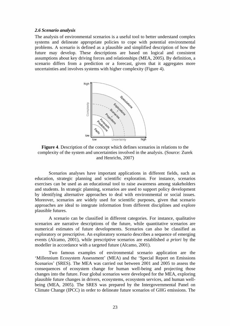
2.6 Scenario analysis
The analysis of environmental scenarios is a useful tool to better understand complex
systems and delineate appropriate policies to cope with potential environmental
problems. A scenario is defined as a plausible and simplified description of how the
future may develop. These descriptions are based on logical and consistent
assumptions about key driving forces and relationships (MEA, 2005). By definition, a
scenario differs from a prediction or a forecast, given that it aggregates more
uncertainties and involves systems with higher complexity (Figure 4).
Figure 4. Description of the concept which defines scenarios in relations to the
complexity of the system and uncertainties involved in the analysis. (Source: Zurek
and Henrichs, 2007)
Scenarios analyses have important applications in different fields, such as
education, strategic planning and scientific exploration. For instance, scenarios
exercises can be used as an educational tool to raise awareness among stakeholders
and students. In strategic planning, scenarios are used to support policy development
by identifying alternative approaches to deal with environmental or social issues.
Moreover, scenarios are widely used for scientific purposes, given that scenario
approaches are ideal to integrate information from different disciplines and explore
plausible futures.
A scenario can be classified in different categories. For instance, qualitative
scenarios are narrative descriptions of the future, while quantitative scenarios are
numerical estimates of future developments. Scenarios can also be classified as
exploratory or prescriptive. An exploratory scenario describes a sequence of emerging
events (Alcamo, 2001), while prescriptive scenarios are established a priori by the
modeller in accordance with a targeted future (Alcamo, 2001).
Two famous examples of environmental scenario application are the
‗Millennium Ecosystem Assessment‘ (MEA) and the ‗Special Report on Emissions
Scenarios‘ (SRES). The MEA was carried out between 2001 and 2005 to assess the
consequences of ecosystem change for human well-being and projecting those
changes into the future. Four global scenarios were developed for the MEA, exploring
plausible future changes in drivers, ecosystems, ecosystem services, and human well-
being (MEA, 2005). The SRES was prepared by the Intergovernmental Panel on
Climate Change (IPCC) in order to delineate future scenarios of GHG emissions. The
Page 24
24
SRES scenarios comprise an extensive range of forces driving GHG emission, from
demographic to technological developments, and accounts for the emissions of all
relevant species of GHGs (IPCC, 2007).
3. DATA
This section provides a brief description of the dataset used in the thesis. Figure 5
illustrates in which research paper each of the datasets was applied. Due to a close
linkage between the studies, some datasets are mutually applied in more than one
research paper.
Figure 5. Illustration presenting an overview of the datasets used in each of the
research papers presented in this thesis
3.1. Remote sensing data
A) Land cover maps derived from SPOT imagery
The land use and land cover of the Taita Hills played a central role in this thesis, in
particular for the papers I, III, IV and V. Land use/land cover maps for the years 1987
and 2003 were created by mapping SPOT 4 HRVIR satellite images (path and row
143-357), with a 20 m spatial resolution and green, red and NIR spectral bands. The
images were orthorectified using a 20 m planimetric resolution DEM. Atmospheric
correction was implemented utilizing the historical empirical line method (HELM).
The SPOT images were classified according to a nomenclature derived using the land
cover classification system protocol of the Food and Agriculture Organization (FAO)
of the United Nations and the United Nations Environment Programme (UNEP) (Di
Gregorio, 2005) (Table 1). The classification methodology utilized a multi-scale
segmentation/object relationship modelling approach implemented with the Definiens
software tool. An accuracy assessment for the 2003 classification was undertaken
based on ground reference test data, independent of the training data, collected during
field visits in 2005/2006 using stratified random road sampling. Additional reference
points for the test data were collected from a 0.5 m resolution airborne true-colour
Page 25
25
digital camera imagery acquired in January 2004. All the procedures describe above
were performed in a previous study carried out by Clark (2010).
Table 1. LCCS nomenclature adopted for SPOT imagery LULC mapping of the Taita
Hills
Land Cover Classes
Cropland
Shrubland and Thicket (>20% Cover with
Emergent Trees)
Woodland
Plantation Forest
Broadleaved Closed Canopy Forest
Grassland with scattered shrubs and trees
Bare Soil and Other Unconsolidated Material
Built-up Area
Bare Rock
Water
B) MODIS land surface temperature
The Moderate Resolution Imaging Spectroradiometer (MODIS) (Justice et al., 2002)
was launched in 1999 and 2002 on board the Terra and Aqua satellites, respectively. It
can provide images in 36 different spectral bands, with spatial resolutions of 250, 500
and 1000 m, depending on the spectral band. The United States National Aeronautics
and Space Administration (NASA), responsible for processing and distributing
MODIS sensor data, makes available a large variety of products for Land, Ocean and
Atmospheric uses.
The MOD11A2 product was used in papers II and V. This product offers
daytime and nighttime Land Surface Temperature (LST) data stored on a 1-km
sinusoidal grid as the average values of clear-sky LSTs during an 8-day period (Wang
et al., 2005). The MODIS LST represents the radiometric temperature related to the
thermal infrared (TIR) radiation emitted from the land surface observed by an
instantaneous MODIS observation (Wan, 2008). The day-time LST corresponds to
measurements acquired around 10:30 am, while night-time LST records are acquired
around 10:30 pm (local solar time).
The MOD11A2 products are validated over a range of representative
conditions, meaning that the product uncertainties are well defined and have been
satisfactorily used in a large variety of scientific studies. This product was extensively
tested using comparisons with in-situ values and radiance-based validation (Wan et
al., 2002; Wan et al., 2004; Wan, 2008). The results of these tests indicate that in most
cases the MODIS LST error is lower than 1 K.
In total, 368 LST images (8-day composite), corresponding to the entire
MOD11A2 product dataset from the years 2001 to 2008, were downloaded from the
Land Processes Distributed Active Archive Center (LP DAAC). The images were
reprojected to the UTM coordinate system (datum WGS84) using the software
MODIS Reprojection Tool (MRT). The temperature values, which are originally in
Page 26
26
Kelvin, were transformed to degrees Celsius in order to fit the models, and the 8-days
composite images compiled into monthly averages.
C) MODIS Normalized Difference Vegetation Index
Normalized Difference Vegetation Index (NDVI) imagery, obtained from the
MOD13Q1 product, were used in paper V. The MOD13Q1 product provides 16-day
composite NDVI imagery from the MODIS Terra and Aqua sensors at 250-meter
spatial resolution (Justice et al., 2002). The MODIS NDVI imagery are computed
from atmospherically corrected bi-directional surface reflectances that have been
masked for water, clouds, heavy aerosols and cloud shadows. In total, 184 images
were used, representing the entire MOD13Q1 product dataset from 2001 to 2008. The
NDVI is widely used to measure and monitor plant growth, vegetation cover and
biomass production. It has the advantage of minimizing band-correlated noises, cloud
shadows, sun and view angles, topography and atmospheric attenuation. The NDVI is
obtained using the following equation:
NDVI =𝜌𝑁𝐼𝑅 −𝜌𝑟𝑒𝑑
𝜌𝑁𝐼𝑅 +𝜌𝑟𝑒𝑑 (1)
3.2 Geospatial landscape attributes
In papers III, IV and V, spatially represented landscape attributes were used in
supporting the analyses. In total, nine attributes were used as inputs for the model,
eight of which were static and one of them was dynamic (distance to croplands).
Static inputs are those that are kept constant throughout the model run, while dynamic
inputs refer to those that undergo changes during the model run. All landscape
attributes were represented by raster layers with a 20 m spatial resolution. The
description of each layer is detailed below:
Distance to Roads: Euclidian distance in meters to the main and secondary
roads. In order to carry out this operation, vector map layers for main roads
were digitized from Kenya‘s 1:50 000 scale topographic maps. The road
network maps were obtained by Siljander (2010).
Distance to Markets: the markets were represented by the main villages in
the region; the distance to markets raster was created by calculating the
Euclidian distance in kilometres to the centre of each village.
Digital Elevation Model: The 20-m spatial resolution DEM was interpolated
from 50-feet interval contours captured from 1:50 000 scale topographic maps,
deriving an estimated altimetric accuracy of ± 8 m and an estimated
planimetric accuracy of ± 50 m (Clark, 2010).
Distance to Rivers: represented by the Euclidian distance in meters to the
main rivers. Two sources were used to extract the river network in the study
area. Firstly, GIS tools were used to automatically identify the rivers based on
a flow accumulation grid obtained using the DEM. Subsequently, eventual
errors in the automatic classification were corrected using a 1:50000 scale
topographic map. The rivers networks were mapped in a previous study
carried out by Siljander (2010).
Page 27
27
Protected Areas: characterized by the national parks and conservation areas
close to the Taita Hills. Namely, a segment of the Tsavo East National Park is
located in the northeastern part of the study area and a small section of the
Taita Hills Game Sanctuary in the southwest.
Soil Type: Soil map obtained from the Soil and Terrain Database for Kenya
(KENSOTER), at scale 1:1M, compiled by the Kenya Soil Survey (Batjes and
Gicheru, 2004).
Slope: slope in percentage extracted from the DEM.
Insolation: Annual average solar radiation in watt hours per square meter
(W.h/m2) for a whole year created from the DEM using ArcGIS 9.3. The
calculations for this landscape attribute were carried out by Siljander (2010).
Distance to Croplands: represented by the Euclidian distance to already
established croplands. This layer was the only dynamic landscape attribute
used as an input for the model, which means that this variable undergoes
changes during the model run as new cropland patches are created.
3.3 Climatic data
A) Observed precipitation
High-spatial-resolution precipitation grids were created by interpolating rainfall
observations from eleven ground stations in the Taita Hills and surrounding lowlands
(Table 2). The data was provided by the Kenya Meteorological Department and the
interpolation procedure was carried out using the ANUSPLINE software (Hutchinson
1995). In total, 17 years of observations, from 1989 to 2005, were used to create
monthly average rainfall maps at a 20 m spatial resolution.
Table 2. Location and name of rainfall gauges
Station Name Station ID Longitude (o) Latitude (o) Altitude (m)
Meteorological Station, Voi 9338001 38.57 -3.40 597
D.C.'S Office, Wundanyi 9338003 38.40 -3.40 1463
Wesu Hospital 9338005 38.35 -3.40 1676
Maktau Railway Station, Maktau 9338007 38.13 -3.40 1099
Taita Sisal Estate LTD, Mwatate 9338012 38.40 -3.55 869
Chief‘s Office, Mgange 9338031 38.32 -3.40 1768
Primary School, Msorongo 9338032 38.22 -3.43 1082
Chief‘s Office, Mbale 9338033 38.42 -3.38 1067
Taita Farmers Training Centre,
Kidaye 9338035 38.35 -3.43 1676
Irima Exclosure, Irima 9338050 38.52 -3.27 610
Kedai Farm , Kedai 9338073 38.37 -3.27 808
Page 28
28
The technique used to interpolate the ground station data is based on tri-variate
functions of longitude, latitude, and elevation to fit thin plate spline functions, which
can be viewed as a generalization of standard multi-variate linear regression. The
degree of smoothness of the fitted function is usually determined automatically from
the data by minimizing a measure of predictive error of the fitted surface given by the
generalized cross validation (Craven and Wahba 1979). The altitude variable
necessary for the function was obtained from a DEM with 20 m spatial resolution
(described in section 4.2).
B) Synthetic precipitation datasets
Climate change scenarios simulated by General Circulation Models (GCMs) generally
provide datasets at spatial resolutions that are considered too coarse for studies at
local scales. Moreover, many spatial downscaling approaches, such as dynamic
downscaling, require additional datasets that are frequently unavailable in developing
countries. Hence, a simplified approach was carried out to generate synthetic
precipitation datasets and simulate plausible climate change scenarios for the study
area.
Firstly, 17 years of monthly average rainfall observations, from 1989 to 2005
(see section 4.3), were used to assess the rainfall statistical distribution in this study
area. The probability distribution function (PDF) for monthly precipitation was
estimated at each point of the grid using a gamma distribution function. The gamma
distribution was chosen for being able to provide flexible representation of a variety
of distribution shapes (Wilks, 1990). Moreover, this type of distribution has been
successfully applied in recent studies to represent monthly rainfall in East Africa
(Husak et al., 2007).
The parameters of the distribution were estimated in the software MATLABTM
using the maximum likelihood approach. After the gamma PDF parameters were
solved for every point in the grid, a Monte Carlo simulation was carried out to
generate synthetic monthly precipitation datasets. For the Monte Carlo simulation,
100 random values were extracted from the PDF in each point of the grid, with each
value representing an estimated monthly volume of precipitation in the respective grid
point. The synthetic precipitation observation in the point is then considered to be the
average of the 100 iterations.
Four synthetic precipitation datasets were generated for this study in order to
simulate different scenarios. In the first scenario (Sy), a synthetic precipitation dataset
was generated by running the Monte Carlo simulation using the same characteristics
observed in the historical dataset (1989 to 2005). In other words, the Sy represents the
monthly precipitations in a scenario without climate change. The Sy scenario is
considered throughout the present study the reference for comparisons with the
climate change scenarios.
In the three other scenarios, climatic changes were simulated by perturbing the
PDF during the Monte Carlo simulation. In order to delineate plausible scenarios, the
PDFs were perturbed based on precipitation responses to climate change (percent
changes) simulated by a GCM between the years 2011 and 2030. Given the coarser
spatial resolution of the GCM, just the GCM grid point closest to the study area was
used as reference for the precipitation response values.
Page 29
29
The GCM chosen for use in this study was the ECHAM version 5, developed
at the Max Planck Institute for Meteorology in Hamburg. In a comparison with five
other GCMs, the ECHAM achieved the best results in simulating the rainfall patterns
in the East-African region (McHugh, 2005). Moreover, the ECHAM5 was
successfully used in recent studies aiming to evaluate the impacts of climate changes
on agricultural systems in East Africa (Thornton et al., 2009; Thornton et al., 2010).
The climate changes simulated by the ECHAM5 for three greenhouse-gas
emission scenarios (SRES, Special Report on Emissions Scenarios) were used as
reference in this study for perturbing the precipitation PDFs. Namely, the emission
scenarios SRA1B, SRA2 and SRB1 (Nakicenovic et al., 2000) were used to generate
three synthetic precipitation datasets: SyA1B, SyA2 and SyB1, respectively. The data
necessary for this procedure were obtained from the IPCC data distribution centre
(http://www.ipcc-data.org).
The SRA1B emission scenario simulates a future world of rapid economic
growth, low population growth and rapid introduction of new and more efficient
technology. The SRA2 scenario represents a very heterogeneous world, with high
population growth, slow technological changes and less concern for rapid economic
development. Lastly, the SRB1 simulates a world with rapid changes in economic
structures toward a service and information economy, with the introduction of clean
and resource-efficient technologies (IPCC, 2007).
C) Synthetic land surface temperature datasets
The calculation of the synthetic temperature datasets followed the same procedure
carried out for defining the precipitation datasets. That is to say, historical
observations were used to assess the variability of the LST in the study area. This
information was used to define the temperature probability distribution function for
each grid point in the study area. The probability distribution functions were applied
to Monte Carlo simulations in order to generate synthetic temperature datasets.
Climate change scenarios were simulated by perturbing the distribution functions
during the Monte Carlo simulation based on temperature responses simulated by a
General Circulation models.
Thus, an important assumption should be highlighted in this approach. The air
temperature changes projected by the GCM were used to perturb the Monte Carlo
simulations in order to represent the respective responses on LST. Therefore, it was
assumed that responses on LST will have similar magnitudes as for the air
temperature.
The probability distribution function used to describe the variability of the
monthly LST in the study area was the normal distribution. The assumption that
temperature is normally distributed is widely used in stochastic weather generation
models (e.g. Semenov and Barrow, 1997; Stockle and Nelson, 1999). Although the
normal distribution may not be ideal to represent daily maximum and minimum
temperatures, studies have shown that it is adequate to reproduce monthly means and
standard deviations (e.g. Harmel et al., 2002).
The scenarios simulated in the synthetic temperature datasets were the same as
for the precipitation datasets. Namely, three datasets were created (SyA1B, SyA2 and
SyB1) based on temperature anomalies simulated by a GCM considering different
greenhouse-gas emission scenarios (SRA1B, SRA2 and SRB1, respectively) for the
Page 30
30
period between the years 2011 to 2030. In this case, the Model for Interdisciplinary
Research on Climate (MIROC3.2) was used as the reference. The MIROC3.2 results
were chosen for being the most appropriate data available at the IPCC data
distribution centre able to provide estimates of maximum and minimum temperatures
for the three greenhouse-gas emission scenarios used in the present study.
4. METHODS
4.1 Alternative approach for agricultural survey planning
An alternative approach to assist agricultural survey in the Taita Hills was evaluated
using an adaptation of the method proposed by Epiphanio et al. (2002). The method
combines statistical analysis with GIS and remote sensing techniques to assist surveys
aiming at crop area estimation. The first step of the approach consisted of applying
remote sensing techniques to identify the areas where agricultural activities are taking
place within the study area. For this, a SPOT 4 HRVIR 1 satellite image, dated 15th
October, 2003, was used in the analysis.
Next, a stratified random sampling scheme was performed using GIS. In the
stratified random sampling, the population is first divided into a number of parts or
'strata' according to characteristics that are considered to be associated with the main
variables being studied. In the particular case of this study, the stratification was
performed by separating the agricultural areas from the remaining land use classes.
Hence, the pixels of the image classified as agricultural area were inserted in a
subpopulation with N members. After the stratification is defined, a random sampling
algorithm is applied to collect n samples inside the subpopulation. The stratified
random sampling is likely to achieve better results than the simple random sampling,
provided that the strata has been chosen so that members of the same stratum are as
similar as possible in respect of the characteristic of interest.
In order to identify the type of crop cultivated in the area represented by each
sample, field work is carried out assisted by GIS and Global Position Systems (GPS)
receivers. After the crop type of each sample is defined, the proportion in which a
determined crop type occurs in n is equivalent to the proportion of this respective crop
type in N (Cochran, 1977).
However, defining an optimal number of samples (n) to be visited in the field
is a challenging task, which is frequently made subjectively. To overcome this
problem, this study carried out a Monte Carlo simulation (Metropolis and Ulam,
1949) prior to the field work. The results of the simulation were used to define the
most suitable sampling strategy taking into account the errors inherent in the analysis
and the time and resources available for the field work. The Monte Carlo method uses
random numbers and probability to solve problems by directly simulating the process.
It may be used to iteratively evaluate a deterministic model using sets of random
numbers as inputs.
The first step in performing the analysis was to assemble a simple model to
simulate field work activities. An image representing a Synthetic Crop Field (SCF)
was generated by creating a matrix with the same number of pixels (N) as observed in
the stratum classified as agricultural areas in Taita Hills. A crop type class was
randomly assigned to each element of the SCF. In order to create a consistent
proportion, the number of classes and the percentage of each class in the SCF were
Page 31
31
based on values acquired from previous surveys carried out by the Kenyan‘ Ministry
of Agriculture.
After setting the SCF, random samples were collected within the matrix, and
used to estimate the proportion of crop types. The number of samples (n) used to
estimate the crop type proportion in the SCF ranged from 10 to 1000. The simulation
was repeated 100 times for each n value. The error in estimating the crop type
proportion was monitored in every iteration. A flowchart illustrating the steps taken in
this research is presented in Figure 6.
Figure 6. Flowchart illustrating the agricultural survey approach assisted by remote
sensing and Monte Carlo simulation.
4.2 Alternative methods for estimating reference evapotranspiration
In order to identify feasible approaches for estimating ETo in the Taita Hills, three
empirical ETo models that require only air temperature data were evaluated, namely
the Hargreaves, the Thornthwaite and the Blaney-Criddle methods.
a) Hargreaves:
The Hargreaves method was developed by Hargreaves et al. (1985), using
eight years of daily lysimeter data from Davis, California, and tested in
different locations such as Australia, Haiti and Bangladesh. The method has
been successfully applied worldwide (e.g. Gavilán et al., 2006). The
Hargreaves equation requires only daily mean, maximum and minimum air
temperature and extraterrestrial radiation.
b) Thornthwaite:
The Thornthwaite method (Thornthwaite, 1948) is based on an empirical
relationship between ETo and mean air temperature. It was initially
developed for the central and eastern regions of the United States, where the
predominant climate is characterized by wet winters and dry summers.
Although the method has been successfully applied in different regions of the
world (e.g. Ahmadi and Fooladmand, 2008; Dinpashoh, 2006), some authors
argue that the method should be carefully applied in regions with climate
characteristics different from the ones where the method was developed.
Page 32
32
c) Blaney-Criddle:
The Blaney-Criddle equation (Blaney and Criddle, 1962) is another early
empirical model developed to estimate ETo. This model was designed for the
arid western portion of the United States and it was demonstrated to provide
accurate estimates of ETo under these conditions. Although it was developed
some decades ago, this method is still successfully applied in many water
management studies (e.g. Fooladmand and Ahmadi, 2009).
To overcome the low data availability from ground stations, this study made
use of LST data obtained from the MOD11A2 product (Wang et al., 2005). In order to
clearly distinguish this approach, when LST data is used in replacement of air
temperature data from ground stations, the Hargreaves, the Thornthwaite and the
Blaney-Criddle models will be hereafter denominated as Hargreaves-LST,
Thornthwaite-LST, and Blaney-Criddle-LST, respectively.
The empirical equations were calibrated using as a reference the FAO
Penman–Monteith (FAO-PM) method. The FAO-PM method is recommended as the
standard ETo method and has been accepted by the scientific community as the most
precise, this is because of its good results when compared with other equations in
different regions worldwide (Cai et al., 2007; Jabloun and Sahli, 2008). Although the
FAO-PM method also carries intrinsic uncertainties and errors, it has behaved well
under a variety of climatic conditions, and for this reason the use of such methods to
calibrate or validate empirical equations has been widely recommended (Allen et al.,
1998; Itenfisu et al., 2003; Gavilán et al., 2006).
The meteorological data necessary for the FAO-PM equations were obtained
from a synoptic station placed at Voi town and operated by the Kenya meteorological
department. ETo values were also calculated for this exact point using the empirical
models and MODIS LST data. The calibration parameters were defined using the
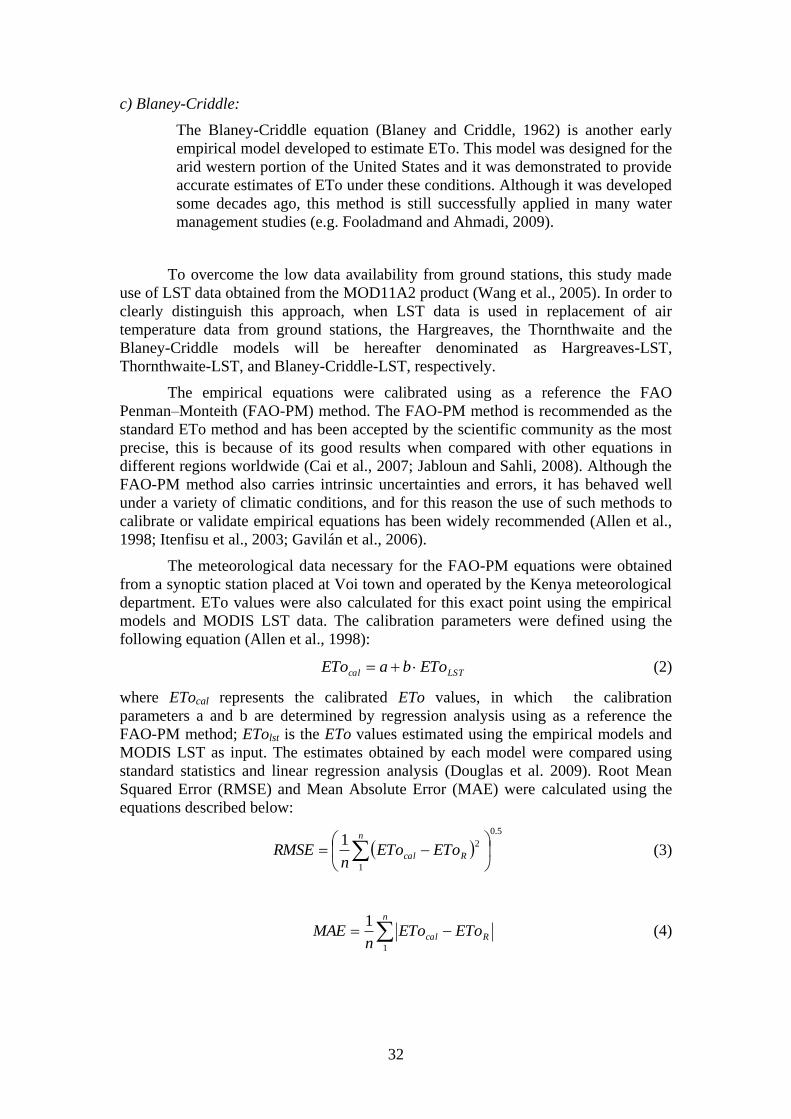
following equation (Allen et al., 1998):
LSTcal ETobaETo
(2)
where ETocal represents the calibrated ETo values, in which the calibration
parameters a and b are determined by regression analysis using as a reference the
FAO-PM method; ETolst is the ETo values estimated using the empirical models and
MODIS LST as input. The estimates obtained by each model were compared using
standard statistics and linear regression analysis (Douglas et al. 2009). Root Mean
Squared Error (RMSE) and Mean Absolute Error (MAE) were calculated using the
equations described below:
5.0
1
21
n
Rcal EToETon
RMSE (3)
n
Rcal EToETon
MAE1
1 (4)
Page 33
33
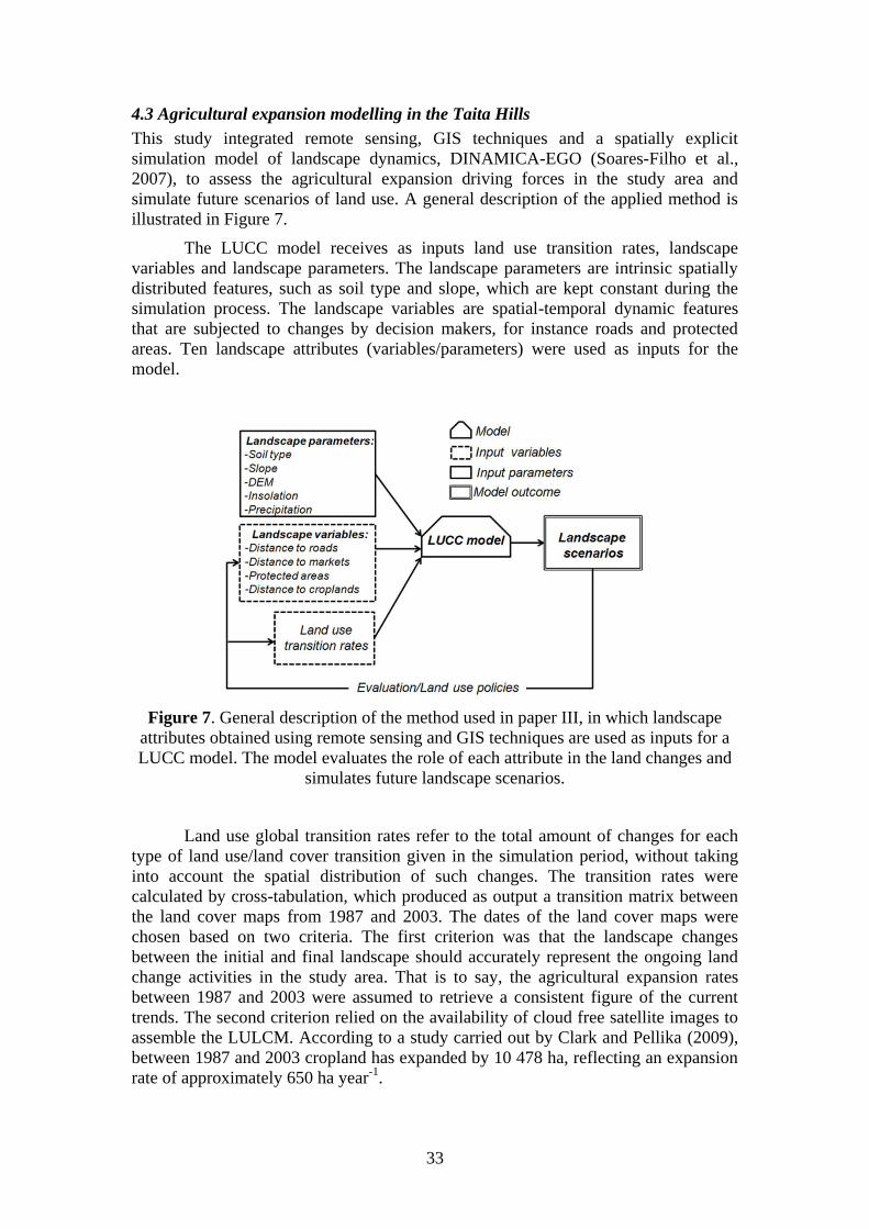
4.3 Agricultural expansion modelling in the Taita Hills
This study integrated remote sensing, GIS techniques and a spatially explicit
simulation model of landscape dynamics, DINAMICA-EGO (Soares-Filho et al.,
2007), to assess the agricultural expansion driving forces in the study area and
simulate future scenarios of land use. A general description of the applied method is
illustrated in Figure 7.
The LUCC model receives as inputs land use transition rates, landscape
variables and landscape parameters. The landscape parameters are intrinsic spatially
distributed features, such as soil type and slope, which are kept constant during the
simulation process. The landscape variables are spatial-temporal dynamic features
that are subjected to changes by decision makers, for instance roads and protected
areas. Ten landscape attributes (variables/parameters) were used as inputs for the
model.
Figure 7. General description of the method used in paper III, in which landscape
attributes obtained using remote sensing and GIS techniques are used as inputs for a
LUCC model. The model evaluates the role of each attribute in the land changes and
simulates future landscape scenarios.
Land use global transition rates refer to the total amount of changes for each
type of land use/land cover transition given in the simulation period, without taking
into account the spatial distribution of such changes. The transition rates were
calculated by cross-tabulation, which produced as output a transition matrix between
the land cover maps from 1987 and 2003. The dates of the land cover maps were
chosen based on two criteria. The first criterion was that the landscape changes
between the initial and final landscape should accurately represent the ongoing land
change activities in the study area. That is to say, the agricultural expansion rates
between 1987 and 2003 were assumed to retrieve a consistent figure of the current
trends. The second criterion relied on the availability of cloud free satellite images to
assemble the LULCM. According to a study carried out by Clark and Pellika (2009),
between 1987 and 2003 cropland has expanded by 10 478 ha, reflecting an expansion
rate of approximately 650 ha year-1
.
Page 34
34
The local transition probabilities, different from the global transition rates, are
calculated for each grid cell considering the natural and anthropogenic characteristics
of the site. The transition probability of each cell was calculated in DINAMICA-EGO
using the weights of evidence (WoE) method (Soares-Filho et al., 2002; Almeida et
al., 2008). The WoE is a Bayesian method in which the effect of each landscape
variable on a transition is calculated independently of a combined solution (Soares-
Filho et al., 2002). The spatial probability of a transition is given by the following
equation (Bonham-Carter, 1994):
t
j
W
W
n
yx
n
i
yx
n
i
eTO
eTOVVVT
1
21yx,
,
1
,
1
}{1
}{}.../{P , (5)
where Px,y is the probability of transition in a cell with coordinates x,y; T represents
the land use/land cover transition; Vn accounts for all possible landscape variables i
selected to explain transition T; O{T} is the odd of a transition, represented by the
ratio between a determined transition probability and the complementary probability
of non-occurrence, described by equation 6:
}TP{
P{T} O{T} , (6)
where P{T} is the probability of occurrence of transition T, given by the number of
cells where the concerned land use/land cover transition occurred divided by the total
number of cells in the study area; P{ T } is the probability of non-occurrence of
transition T, given by the number of cells where the concerned land use/land cover
transition is absent divided by the total number of cells in the study area, and W+
x,y is
the weight of evidence for a determined landscape variable range, defined by the
following equation:
}/{
}/{log
TViP
TViPW e , (7)
where P{Vi /T} is the probability of occurring variable Vi in face of the previous
presence of transition T, given by the number of cells where both Vi and T are found
divided by the total number of cells where T is found and P{Vi /T } accounts for the
probability of occurring variable Vi in face of the previous absence of transition T,
given by the number of cells where both Vi and are found divided by the total
number of cells where T is not found.
The W+ values represent the attraction between a determined landscape
transition and a certain variable. The higher the W+ value is, the greater is the
probability of a certain transition to take place. On the other hand, negative W+ values
indicate lower probability of a determined transition occurring in the presence of the
respective variable range. Based on the W+ values of each range for every considered
variable, DINAMICA-EGO generates a spatially explicit probability map, in which
the cell receives as attributes the probability for a determined transition.
After defining the weight of each landscape variable, transition probability
maps are created for every simulated year. Based on spatial probabilities, new
agricultural patches are stochastically allocated using two algorithms: ―expander‖ and
Page 35
35
‗patcher‘. The expander function performs the expansion of previously existing
patches of a certain class. The patcher function, in turn, is designed to generate new
patches through a seed formation mechanism (Soares-Filho et al., 2002).
The model performance was evaluated using an adaptation of the method
proposed by Hagen (2003) in which multiple resolution windows are used to compare
the simulated and the reference maps within a neighbourhood context. Approaches
considering neighbourhood contexts are useful in comparing maps that do not exactly
match on a cell-by-cell basis, but still present similar spatial patterns within certain
cell vicinity (Soares-Filho et al., 2002). The method retrieves a fuzzy similarity index
defined within a window that is gradually expanded, allowing the assessment of the
model‘s performance at multiple resolutions. This fuzzy similarity index is based on
the concept of fuzziness of location, in which a representation of a cell is influenced
by the cell itself and by the cells in its vicinity (Hagen, 2003). The degree of similarity
for each pixel is represented on a scale of 0 to 1, where zero represents total
disagreement and one represents identical maps.
4.4 Assessment of potential impacts on soil erosion
Future agricultural expansion and climate change scenarios were used in order to
evaluate their potential impacts on soil erosion in the Taita Hills. To achieve this
objective a modelling framework was assembled by coupling a landscape dynamic
simulation model, an erosion model and synthetic precipitation datasets generated
through a Monte Carlo simulation (section 3.5). This approach aimed to evaluate how
agricultural expansion, together with climate change, can modify the variables of a
widely used soil erosion model, allowing a qualitative assessment of the impacts of
these changes for soil conservation.
The soil erosion model used was the Universal Soil Loss Equation (USLE)
(Wischmeier and Smith, 1978). Remote sensing and GIS techniques were combined
to provide the necessary inputs for the modelling framework. A flow chart illustrating
the components of the modelling framework is presented in Figure 8.
Figure 8. Flow chart illustrating the integrated modelling framework concept used in
paper IV.
Page 36
36
The USLE and its revised version, RUSLE (Renard et al., 1997), have been
extensively used worldwide during the last decades (Kinnell, 2010). Even though
these models are known for their simplicity, their effectiveness has been demonstrated
in many recent studies (e.g. Beskow et al., 2009; Terranova et al., 2009; Nigel and
Rughooputh, 2010), including several studies in Kenya (e.g. Angima et al., 2003;
Mutua et al., 2008). The USLE is given as:
𝐴 = 𝑅 × 𝐾 × 𝐿𝑆 × 𝐶 × 𝑃 (8)
where A is the annual average soil loss [t ha–1
ano–1
], R is the rainfall erosivity factor
[MJ mm ha–1
h–1
], K is soil erodibility [t ha h MJ–1
mm–1
], L and S are the
topographical factor [-], C is the vegetation cover factor [-], and P represents erosion
control practices [-].
Provided the fact that the K and LS factors are intrinsic characteristics of the
landscape, they can be kept constant in all simulated scenarios. On the other hand,
land changes directly affect the C factor. These changes were analysed by evaluating
the average C factor value in the study area during 1987, 2003 and in the simulated
scenario for 2030. The potential impacts of agricultural expansion for soil
conservation were also assessed by analysing the spatial distribution of croplands in
relation to the K and LS factors. Possible changes on the P factor were not addressed
in the present study.
The rainfall erosivity factor (R) is a numerical index that expresses the
capacity of the rain to erode a soil (Wischmeier and Smith, 1978). Hence, the R factor
is directly affected by changes in precipitation pattern. These changes were evaluated
at monthly and yearly time steps. Additionally, the soil erosion potential was
calculated by excluding the anthropogenic variables from the USLE equation (C and
P). This approach is needed to clearly understand the role of external factors in the
system without the influence of the changes in the landscape cause by human
activities.
Although the USLE provides a simple and useful tool for soil conservation,
studies commonly neglect the calibration and validation of this model. Given the
absence of reliable data for calibration, the presented study did not attempt to provide
soil loss estimation figures. Instead, the evaluation of the soil erosion potential among
the different scenarios was based mainly on a comparative analysis of changes,
following the procedure proposed by Kepner et al. (2004) and Miller et al. (2002).
Such procedure assumes that, using percent change observations, the parameters
incorporated in an eventual calibration would be partially or totally cancelled,
providing more realistic figures than absolute values of soil loss. The absolute
changes in soil erosion potential were analysed only qualitatively, taking into account
the spatio-temporal distribution of changes.
The R factor was calculated using the method proposed by Renard and
Freimund (1994), and recently applied by Beskow et al. (2009). The method is based
on an empirical relationship between rainfall erosivity and the Fournier Index (FI).
The FI (Fournier 1960) indicates climatic aggressiveness, which has a high
correlation with the amount of sediment washed into the stream by surface runoff.
The K factor was calculated using the method proposed by Williams and
Renard (1983). This approach was chosen for being broadly used in recent studies
(e.g. Xiaodan et al., 2004; Rahman and Chongfa, 2009) and for requiring input
variables that are commonly available worldwide. The data necessary for calculating
Page 37
37
the K factor were obtained from the Soil and Terrain Database for Kenya
(KENSOTER), which provides a harmonized set of soil parameter estimates for
Kenya (Batjes and Gicheru, 2004).
The topographical factor (LS) was calculated in the software USLE2D (Van
Oost et al., 2000), using the algorithm proposed by Wischmeier and Smith (1978).
This calculation was performed based on a 20 m spatial resolution DEM.
4.5 Assessment of potential impacts on irrigation water requirement
In this last investigation, agricultural expansion and climate change scenarios were
used to evaluate their potential impacts on Irrigation Water Requirements (IWR).
Remote sensing and GIS techniques were combined to provide the necessary inputs
for the modelling framework described in Figure 9.
Figure 9. Flow chart illustrating the integrated modelling framework concept used in
paper V.
Crop water requirement (CWR) is defined as the amount of water required to
compensate the ET loss from a cropped field (Allen et al., 1998). In cases where all
the water needed for optimal growth of the crop is provided by rainfall, irrigation is
not required and the IWR is zero. In cases where all water has to be supplied by
irrigation the IWR is equal to the crop ET (ETc). However, when part of the CWR is
supplied by rainfall and the remaining part by irrigation, the IWR is equal to the
difference between the ETc and the Effective Precipitation (Peff). In such cases, the
IWR was computed using the following equation (FAO, 1997):
mmmm PeffEToKcIWR 30 (9)
where: IWRm = monthly average crop water requirement in month m, [mm]; Kcm=
crop coefficient in month m, [-]; ETom= mean daily reference evapotranspiration in
month m, [mm day-1
]; Peffm = average effective precipitation in month m, [mm].
Page 38
38
The Peff is defined as the fraction of rainfall retained in the root zone, which
can be effectively used by the plants. That is, the portion of precipitation that is not
lost by runoff, evaporation or deep percolation. The monthly total rainfall was
converted to Peff using a simplified method proposed by Brouwer and Heibloem
(1986), which is based on empirical observations and requires only the total monthly
volume of precipitation.
Based on the results obtained in paper II, the Hargreaves model was chosen to
estimate the ETo in the study area. The Kc values were obtained from tables
recommended by FAO (Allen et al., 1998). Nevertheless, to assign the appropriate Kc
values it is essential to identify the agriculture calendar in the study area, that is, the
period of the year when crops are planted, grown and harvested. For this, monthly
NDVI obtained from MODIS imagery were used to identify the phenological stages
of croplands during the year.
5. RESULTS
5.1 Agricultural survey strategy based on Monte Carlo simulations
Figure 10 shows the results of the simulations carried out to estimate the proportion of
the hypothetical crop types 1, 2, 3, 4 and 5 in the SCF using different number of
samples.
Page 39
39
Figure 10. RMSE retrieved from the Monte Carlo simulation using a number
of samples from 10 to 1000.
The total average RMSE ranged from around 10%, using 10 samples, to less
than 1%, when 1000 samples were used to estimate the crop type‘s proportion in the
SCF. In general, it is noted that the predominant crops (1 and 2) retrieved higher
RMSE, although the error curve in both cases followed the same trend observed in the
other crops. The trend line that best fits all regressions can be described by an
exponential function. The exponential regression between the total average RMSE
and the number of samples achieved a coefficient of determination (R2) of 0.985.
Based on the error curves showed in Figure 10, 300 random points were
distributed in the areas classified as croplands. These points were visited during field
work and the gathered information processed in a spreadsheet to calculate the
proportion of each crop type. The results were consistent with previous agricultural
surveys carried out by the Kenyan‘ Ministry of Agriculture and could properly reflect
the current trends observed in the field. Maize and beans continue to be the
predominant crops in the region. Cassava, cowpeas and pigeon peas are also
cultivated throughout Taita Hills, although in a lower proportion.
Page 40
40
5.2 Remote sensing based methods for estimating evapotranspiration
The results obtained in the evaluation of the ETo models are summarized in Table 3.
The global average RMSE and MAE are fairly homogeneous for each of the
evaluated models. The RMSE ranged from 0.47 mm day-1
, with the Hargreaves-LST
model, to 0.53 mm day-1
, with the Blaney-Criddle-LST model. The MAE achieved
similar figures, ranging from 0.39 mm day-1
, with the Hargreaves-LST model, to 0.46
mm day-1
, with the Blaney-Criddle-LST model.
Table 3. Summary of the results obtained from the models‘ error analysis and linear
regression analysis
Hargreaves-
LST
Thornthwaite-
LST
Blaney-Criddle-
LST
Correlation coefficient (R) 0.67 0.66 0.55
RMSE (mm day-1
) 0.47 0.49 0.53
MAE (mm day-1
) 0.39 0.42 0.46
Calibration parameter (a) 3.221 3.507 -1.980
Calibration parameter (b) 0.497 0.543 1.379
The monthly errors obtained by the tested models, in comparison with the
reference method, are presented in Figure 11. Although the monthly performance of
the models is uniform between March and July, important differences are observed in
January, February and between August and December (Figure 11). In particular for
the Blaney-Criddle-LST model, it is possible to notice a clear increase of the RMSE
and MAE in January, November and December. The Blaney-Criddle-LST model
performed better in months when air temperature was closely related to LST, but had
its performance reduced in months when air temperature and LST are less correlated.
However, the Hargreaves-LST model was more efficient in minimizing the effects of
the differences observed between air temperature and LST during November,
December and January. The model performed well during these months, retrieving
RMSEs of 0.51, 0.61 and 0.51 mm day-1
, respectively.
Figure 11. Root Mean Squared Error (RMSE) and Mean Absolute Error (MAE). The
errors are used to quantify the differences between the ETo estimated using the
reference method (FAO-PM) and the estimates obtained using the empirical models
parameterized using MODIS LST data.
Page 41
41
Considering the results achieved in this study and comparisons with previous
research, it is concluded that the Blaney-Criddle-LST model is not appropriated for
this region when using the proposed methodology. However, the Hargreaves-LST
model achieved the best results in the linear regression and in the analysis of errors.
The results obtained using the Hargreaves-LST are compatible with the errors
observed by Gavilán et al. (2006), which evaluated the Hargreaves equation under
semiarid conditions in southern Spain, finding RMSE ranging from 0.46 to 1.65 mm
d-1
. Furthermore, the correlation coefficients obtained by the Hargreaves-LST and
Thornthwaite-LST models are consistent with the results reported by Narongrit and
Yasuoka (2003), which achieved R2 of 0.57 and 0.60 when comparing these
respective models with the FAO-PM method.
5.3 The driving forces of agricultural expansion and scenarios for 2030
The annual average agricultural expansion rates observed from 1987 to 2003 are
shown in Table 4. The highest conversion rates were observed in the transition from
woodlands to agriculture. However, considering absolute numbers, shrubland areas
are the most affected, given that currently they represent the predominant vegetation
type in the region. The small regions covered with broadleaved forests were nearly
untouched, presenting low conversion rates, the total area decreased from 7.7 to 6.9
km2 during the observed period.
Table 4. Annual average agricultural expansion rates (baseline 1987-2003)
Original vegetation Annual conversion rate
(%) (baseline 1987-2003)
Shrubland 1.305
Woodland 2.013
Plantation forest 1.161
Broadleaved forest 0.289
Grassland 0.310
The most relevant W+ values obtained during the model calibration are shown in
Figure 12. This information represents the attraction between a determined landscape
transition and a certain landscape attribute. Distance to rivers, insolation, distance to
croplands, DEM, distance to roads and distant to markets were particularly associated
with the land-use transitions. The distance to croplands is an important driving factor
for all transitions indicating that the proximity to previously established croplands is a
key factor for agricultural expansion in this region.
Although areas close to rivers did not retrieve high positive W+ values, the
importance of water bodies for croplands is clearly reflected in regions distant fom
rivers, where high negative W+ values are observed. Hence, the results indicate that
patches further than 1 km from water bodies have lower probability of being
converted to cropland. Distance to roads also presents a clear pattern in influencing
the transition from shrublands to croplands. Nevertheless, this attribute did not
retrieve very high W+ values, possibly due to the fact that the Taita Hills comprise a
Page 42
42
relatively dense road network, diminishing the contrast between areas nearby and
away from roads. The distance to markets, here represented by the Euclidean distance
to the main villages, was the most representative driving force for the agricultural
expansion.
Figure 12. W+ values attributed for each range of six landscape attributes most
related to the ‗shrublands to croplands‘ transition.
After the model is calibrated and the role of each landscape variable is defined,
transition probability maps are created for each simulated year. The spatial
probabilities are used to guide the distribution of new simulated agricultural patches,
which are stochastically allocated by the ‗expander‘ and ‗patcher‘ algorithms. In
Page 43
43
Figure 13, the land use maps for 1987 and 2003 are displayed (upper left and upper
right) together with the land use maps for 2030 resulted from the BAU and GOV
scenarios simulations (lower left and lower right). It is observed that, in 1987,
croplands were already clearly established along highlands (central area in the maps).
This is explained by the favourable climatic and edaphic conditions for agricultural
activities (e.g. high precipitation rates), which resulted in the clearance of large areas
of forest during the last century.
In the BAU scenario, the cropland areas expanded to around 515 km2 in 2030,
corresponding to about 60% of the study area. This represents an increase of 40% in
comparison to the year 2003, when croplands occupied around 365 km2. Although the
effects of the governance scenario cannot be easily identified in the map shown in
Figure 13, the simulated land use policies resulted in a significant reduction of the
agricultural expansion. The total area used for agriculture in 2030 for the GOV
scenario was approximately 485 km2.
Figure 13. Land use maps for 1987 and 2003 (upper left and upper right) and
simulated scenarios for 2030 (lower left and lower right).
5.4 Potential impacts on soil erosion by 2030
The results show that agricultural patches established during the last decades were
carefully settled in areas with favourable topography from the soil conservation
perspective, i.e. lower LS factor. This pattern was reinforced after 1987, when the
availability of space in the hills was scarce and the agriculture started expanding to
flat areas along the foothills. In the agricultural expansion simulated for 2030, a slight
Page 44
44
increase is noted in cropland patches settled in areas with LS factor between 1 and 10,
whereas the most significant increase was again in areas with a topographic factor
between 0 and 1.
The soil erodibility factor in the study area varied from 0.0139 to 0.0307,
allowing the distinction of eight different erodibility classes. Because soil erodibility
figures may vary according to the method used for calculation, the results were
analysed only in a comparative base, taking into account the soil erodibility range
found in the study area. In 1987 and 2003 agricultural areas were established mainly
in soils with medium erodibility (0.0205-0.0255). The simulated agricultural
expansion for 2030 was also higher in these soils. The low occurrence of agricultural
activities in soils with higher erosivity is explained firstly by the low area occupied by
these soils in the study area and secondly by the fact that such soils, together with
climatic variables, create unfavourable conditions for agricultural practices.
Therefore, the results indicate that agricultural activities are unlikely to expand into
areas with higher soil erodibility.
The average R factor for the study area was approximately 3040 MJ mm ha-1
h-1
year-1
when considering the Sy scenario, which simulates the historically observed
precipitation variability. This result is consistent with figures obtained in other semi-
arid regions. Da Silva (2004) found that erosivity varied from 2000 to 4000 MJ mm
ha-1
h-1
year-1
in semi-arid regions in the north-east of Brazil. However, in regions
with high topographic heterogeneity, such as the Taita Hills, it is crucial to consider
local variations at detailed spatial scales.
The erosivity values obtained in the SyA2 scenario resulted in the most
evident differences in comparison with the Sy scenario. In January, March, May and
December the changes in precipitation resulted in a clear but slight decrease in rainfall
erosivity. The erosivity reduction during these months varied from 4 to 120 MJ mm
ha-1
h-1
month-1
. However, still for the SyA2 scenario, a large increase was observed
in April (280 MJ mm ha-1
h-1
month-1
) and November (260 MJ mm ha-1
h-1
month-1
).
For the SyB1 scenario, the increases in rainfall erosivity during April and
November were lower, approximately 217 and 40 MJ mm ha-1
h-1
month-1
,
respectively. A slight decrease was also observed during March, May and December,
but in contrast with the SyA2 scenario, the erosivity during January was almost
constant, with a minor increase of 27 MJ mm ha-1
h-1
month-1
. The SyA1B was the
most conservative scenario, although clear changes are still present. Namely, it
showed the highest erosivity increases during January and December, while it
confirmed the tendency of a decrease in erosivity during March and May.
In general, it is plausible to assert that the climate changes simulated for the
study area are likely to decrease rainfall erosivity during March and May due to a
slight reduction in precipitation rates in these months. However, the model indicates
the possibility of an increase, of much higher magnitudes during April and November.
The disagreements between the simulated scenarios in January and December indicate
higher uncertainties during these months. For June, July, August and September
rainfall erosivity values are likely to continue to be very low.
For all simulated scenarios it is noted that low or no change occurs in the
lowlands (roughly 500 m above sea level). The changes, however, start to be more
evident along areas higher than 1000 m a.s.l., where precipitation rates are historically
higher. In particular for the SyA2 scenario, changes are very high above 1500 m,
Page 45
45
reaching absolute differences up to 1500 MJ mm ha-1
h-1
year-1
when compared with
the Sy scenario.
5.5 Potential impacts on irrigation water requirement by 2030
Spatial and temporal variations on ETo are strong both in the lowlands and in the
hills. In general ETo is higher in the months of September and October, and reaches
the lowest values between April and June. The correlation between ETo and altitude
varies according to season and altitude range. ETo follows more closely the changes
in the altitude in October than in May. In May, the variation ranges from 4.5 to 5.4
mm day-1
while in October the variation is from 5.3 to 6.9 mm day-1
. From 1987 to
2003, a large number of cropland patches were created in areas with ETo between 5.7
and 5.9 mm day-1
, while few new patches were implemented in areas with lower ETo
(<5 mm day-1
). This tendency was strongly sustained during the scenario simulated
for 2030. Hence, it is feasible to assert that by 2030 new croplands are likely to take
place in areas where ETo values are historically higher.
Considering an invariable climate condition (Sy scenario), the agricultural
expansion observed between 1987 and 2003 resulted in an IWR increase of 42%. An
integrated analysis of this result with the historical precipitation volumes in the study
area indicates that the agricultural expansion has likely reached unsustainable levels
from the water resources point of view. That is to say, by 2003 the annual average
precipitation volume in the entire study area (~390 million m3 year
-1) was already
insufficient to meet the water resource requirements necessary to achieve optimal
crop production in every agricultural property.
Among the scenarios simulated for 2030, the Sy scenario resulted in the
highest annual IWR volume, reaching approximately 610 million m3 year
-1. All the
climate change scenarios (SyA1B, SyA2 and SyB1) caused a slight reduction in the
IWR when compared with the Sy scenario. Therefore, the results indicate that the
climate change tendencies up to 2030 are likely to decrease the total annual volume of
IWR in this study area. A comparison between the annual IWR maps for 1987, 2003
and 2030, considering they Sy scenario, is presented in Figure 14.
Figure 14. Annual irrigation water requirement maps for 1987, 2003 and 2030,
considering the Sy scenario. The black areas in the map represent regions where no
agricultural activities are taking place.
Page 46
46
Figure 15 shows the monthly IWR values for all simulated scenarios. The
increase in IWR caused by the agricultural expansion component is clearly identified
in an offset of the curves among different years. Considering only the curves for the
year 2030, the climate changes simulated in the SyA1B, SyB1 and SyA2 datasets
indicate a tendency of increase in the IWR during March and May when compared
with the Sy scenario. This tendency is inverted in April and November, when a slight
decrease is observed in the IWR. During the other months, the IWR is kept relatively
constant among the different climate scenarios. In these cases, eventual increases in
the temperature were likely to be compensated by increases in rainfall volume,
keeping the IWR constant. From the practical point of view, the results indicate a
higher water demand during the seeding season, in February/March, and during the
period of maximum development of the crops, in May. Climate changes are likely to
decrease the water demand for irrigation during both crop growing seasons in April
and November.
Figure 15. Monthly irrigation water requirements volume for the entire study area
during the years 1987, 2003 and 2030. For the year 2030, four climate scenarios are
considered.
6. DISCUSSION
The Taita Hills are among the most degraded areas in the Eastern Arc Mountains,
having lost approximately 99% of their original forest during the last few centuries
(Pellikka et al., 2009). Although this number may sound discouraging, it also makes
the Taita Hills a unique learning environment for the protection of more preserved
areas in the Eastern Arc, such as Udzungwas, East Usambaras and Ulugurus.
Therefore, the causes behind this massive forest loss must not be ignored. In
particular, the fact that these highlands have significant importance for providing food
and income to local population should be acknowledged.
Previous studies have clearly shown that agriculture was the main cause of
forest conversion in the Taita Hills (e.g. Clark, 2010). Consequently, it is already
Page 47
47
known that agricultural activities are actively present in the Taita Hills, and continues
to expand. Nevertheless, the answers for other important questions remain unclear or
unsolved. To better understand the degradation process in the Eastern Arc it is
essential to determine what type of agricultural activities are taking place, to where it
may expand in the future and what impacts it will cause. The combined results of this
thesis provide initial arguments to deal with these important questions.
This thesis proposes an alternative method for agricultural survey in the Taita
Hills, which provides instruments for controlling and planning the survey activities.
The major contribution of the results lies in the possibility of significantly reducing
costs and uncertainties in the survey. In regions with limited technical and financial
resources, such as the Taita Hills, these changes have large potential to quickly
improve availability and reliability of the data provided by local authorities. The
agricultural survey is a fundamental step to characterize agricultural activities.
Knowing what is being cultivated provides additional instruments to identify the
reasons of agricultural expansion and, therefore, it can be considered a tool for
environmental conservation. On the other hand, the information retrieved from
agricultural surveys is also essential for food security and economic planning, given
that it can inform authorities and experts whether or not farmers are planting crop
varieties that are appropriate for current and future climate conditions. Furthermore, a
consistent survey can provide an estimation of nutrients that are lacking for the proper
nutrition of the population, therefore it can provide directions for food subsidy
policies to combat food insecurity.
Besides knowing what is being cultivated, public policies need to take into
consideration the areas where agriculture is more likely to expand in the future. The
answer for this question can only be answered through a detailed assessment of the
forces driving the land changes. In this context, this thesis presents a pioneer
assessment of the driving forces of agricultural expansion in the Taita Hills. The
results obtained in this analysis closely agree with previous studies carried out in
other locations in Kenya. For instance, studying the Narok District in Kenya, Serneels
and Lambin (2001) found that the expansion of small-holder agriculture is mainly
controlled by proximity to permanent water, land suitability and vicinity to villages.
In another similar study, Mertens and Lambin (2000) designed a spatially explicit
model driven by a spectrum of socio-economic and infrastructure variables to
simulate deforestation in southern Cameroon. According to the authors, in this study
case results suggest that roads mostly increased the accessibility of the forest for
migrants rather than providing incentives for the establishment of market oriented
farming systems.
Comparisons with previous studies also highlight the fact that, although many
similarities are evident at large scales, some characteristics of the landscape dynamic
are intrinsic and can only be assessed locally. According to Lambin et al. (2003), land
changes are in general caused by multiple interacting factors, which vary in time and
space, according to specific human-environment conditions. In this context,
similarities and disparities are observed when comparing the driving forces in the
Taita Hills with agricultural expansion areas in other tropical forests. For instance, in
the rain forests of South America, distance to roads and distance to markets arise as
common factors affecting croplands expansion (Aguiar et al., 2007). On the other
hand, in contrast to the industrial agricultural activities in the Brazilian Amazon, new
cropland patches in the Taita Hills are predominantly small, targeting subsistence or
local production. New cropland patches in the Taita Hills were found to have an
Page 48
48
average size of 3 ha, with a variance of 10 ha, while in the agricultural expansion
areas in São Felix do Xingu, Brazilian Amazon, new agricultural patches have an
average size of 300 ha, with a standard deviation of 22.3 ha (Ximenes et al., 2008).
In addition to delineating agricultural expansion scenarios for the year 2030, this
thesis also addressed potential environmental impacts caused by land changes. It is
worth mentioning that due to the particular characteristics of the Taita Hills, the
impacts of environmental changes on natural resources must be carefully analysed.
The highlands of Kenya and Tanzania are considered natural water towers, given that
the higher precipitation rates in these areas historically provide water resources for
large regions along the lowlands throughout the year (Aeschbacher et al., 2005;
Viviroli and Weingartner, 2008). However, the results presented in this study, and
confirmed by field work observations, indicate that the average precipitation rates in
the Taita Hills are no longer able to provide water resources for the lowlands during
the entire year. It is plausible to consider that the changes observed in water resources
availability in the Taita Hills are likely to be caused by two main factors. Firstly, the
increasing use of water resources for irrigation in the hills might be causing a decrease
in rivers‘ flow, diminishing or in some case depleting the volume of water in the
downstream portion of the rivers. The second, but not less important, factor
contributing to this issue is likely to be related to changes in the hydrological response
of the rivers‘ basins caused by the replacement of natural vegetation in favour of
croplands. Previous studies have shown that land changes may increase surface runoff
(e.g. Germer et al., 2010; Githui, et al., 2009) and have direct impacts on water
balance (e.g. Li et al., 2009). These factors can potentially reduce water retention in
the watershed, decreasing the flow during the dry seasons.
The replacement of natural vegetation cover will also contribute for
accelerated soil erosion. Therefore, the undertaken soil conservations practices must
be set as a priority action in the Taita Hills. Although changes in erosion control
practices (P factor) were not considered in this study, previous investigations have
shown that appropriate land management can significantly decrease soil erosion. For
instance, studying soil erosion risk scenarios in Calabria, southern Italy, Terranova et
al. (2009) show that erosion control practices can cause a significant reduction of the
erosive rate, decreasing from roughly 30 to 12.3 Mg ha-1
year-1
. Feng et al. (2010)
demonstrated that soil conservation measures taken by the Chinese government
(Grain-for-Green project) significantly decreased soil erosion in the Loess Plateau
between the years 1990 and 2005.
Finally, it is important to mention that the issues addressed in this thesis
involving water resources and soil conservation can and should be tackled in an
integrated manner. For instance, the adoption of practices to reduce surface runoff,
such as terraces, is an important step to avoid soil erosion, and at the same time it
enhances water infiltration into the soil, allowing a better recharge of groundwater
reservoirs. Furthermore, opting for cultivars capable of maintaining some vegetation
protection over the soil for longer periods can contribute to avoiding the direct impact
of rainfall in the soil and improve soil structure. These factors not only reduce soil
erosion, but also contribute to lower soil evaporation rates and a better water
infiltration. In this context, the consolidation of agroforestry systems using native
plant species may be highly beneficial to the local agriculture, and an excellent
alternative for replacing the eucalyptus plantation forests in the Taita Hills.
Page 49
49
7. CONCLUSIONS AND FURTHER STUDIES
Two general contributions can be highlighted from the results obtained in this thesis.
The first contribution lies in the development and assessment of alternative
approaches to improve the acquisition of data related to key aspects of agricultural
activities in the Taita Hills. The second, but not less important contribution, relates to
the establishment of novel knowledge by delineating unprecedented insights on future
environmental scenarios for the region. Considering the above contributions, the
results of this thesis have a large potential to attain researchers, policy makers and
local population.
A simple and effective approach is proposed to improve the sampling strategy
for agricultural survey in the Taita Hills. By integrating GIS, remote sensing and a
Monte Carlo simulation, the method decreases the uncertainties and costs involved in
the agricultural survey. It was shown that the average RMSE in estimating crop types‘
proportion can vary from around 10%, using 10 samples, to less than 1%, when 1000
samples are used. Nevertheless, despite the clear indications that the method retrieved
appropriated results, further investigations are necessary to perform a detailed
validation. For this, the results obtained in the presented research should be compared
with upcoming reports from the Kenyan‘ Ministry of Agriculture and the possible
sources of errors and uncertainties investigated.
Furthermore, an alternative method for estimating ETo was evaluated by
integrating remote sensing data and empirical models. The combined use of the
Hargreaves ETo model and MODIS LST data retrieved an average RMSE close to 0.5
mm d-1
. This outcome is consistent with results obtained by previous studies reported
in the literature using weather data collected by ground stations. Moreover, the errors
and uncertainties identified in the use of remote sensing LST can be tolerated
considering the reduced weather data collection network in this region. Further studies
are necessary to expand this method for other regions in East-Africa. In particular, the
spatial variability of the calibration parameters for different climate conditions over
East-Africa needs to be identified. Moreover, the method can be significantly
improved by using low cost direct methods (e.g. lysimeters) to calibrate the empirical
equations.
In relation to the agricultural expansion modelling in the Taita Hills, a
connected relation between villages and roads is evident in the definition of new
cropland patches. The proximity to already established crop fields is also one of the
key factors driving the agricultural expansion. If current trends persist, it is expected
that agricultural areas will occupy 60% of the study area by 2030. LUCC simulations
indicate that agricultural expansion is likely to take place predominantly in lowlands
and foothills throughout the next 20 years. Current trends indicate that the small
residual areas of tropical cloud forest, home to a great part of the biodiversity in the
Taita Hills, is likely to remain intact throughout the coming years. Nevertheless, the
impact of the increasing habitat fragmentation in such biodiversity is a relevant issue
that must be addressed in further studies.
The replacement of shrublands and woodlands in favour of croplands expected
for the next decades is very likely to reduce the vegetation cover protecting the soil
against the direct impact of rainfall, resulting in accelerated soil erosion. By the year
2030, rainfall erosivity is likely to increase during April and November. All scenarios
converge to a slight erosivity decrease tendency during March and May. The highest
uncertainties were observed in January and December, when some scenarios indicate
Page 50
50
a small reduction in erosivity while some indicate an increase. Accounting for land
changes and climate changes in an integrated manner, it is plausible to conclude that
the highlands of the Taita Hills must be prioritized for soil conservation policies
during the next 20 years. Although new croplands are likely to be settled in lowlands
over the next decades, increases in precipitation volumes are expected to be higher in
highlands. Moreover, it was demonstrated that in areas with elevated LS factor,
typically in the highlands, increasing rainfall will have significantly higher impacts on
soil erosion potential.
Due to the very limited availability of non-agricultural land in the highlands,
new cropland areas are being settled in areas with low precipitation and higher
temperatures. The continuity of this trend is likely to drive agricultural lands to areas
with a higher IWR, increasing the spatial dependence on distance to rivers and other
water bodies. Although the simulated scenarios indicate that climate change will
likely increase annual volumes of rainfall during the following decades, IWR will
continue to increase due to agricultural expansion. By 2030, new cropland areas may
cause an increase of approximately 40% in the annual volume of water necessary for
irrigation.
Page 51
51
REFERENCES
Aeschbacher, J., Liniger, H., Weingartner, R., 2005. River Water Shortage in a
Highland–Lowland System. Mountain Research and Development 25(2), 155–
162.
Aguiar, A.P.D., Câmara, G., Escada, M.I.S., 2007. Spatial statistical analysis of land-
use determinants in the Brazilian Amazonia: exploring intra-regional
heterogeneity. Ecological Modelling 209(2-4), 169-188.
Alcamo, J., 2001. Scenarios as tools for international environmental assessments,
Experts corner reports - Prospects and Scenarios No 5. European Environment
Agency, Copenhagen.
Allen, R.G, Pereira, L.S., Raes, D. and Smith,M., 1998. Crop evapotranspiration -
Guidelines for computing crop water requirements - FAO Irrigation and
drainage paper 56, FAO, Rome.
Almeida, C.M., Gleriani, J.M., Castejon, E.F., Soares-Filho, B.S., 2008. Using neural
networks and cellular automata for modeling intra-urban land use dynamics.
International Journal of Geographical Information Science 22(9), 943-963.
Alves, D.S., Skole, D.L., 1996. Characterizing land cover dynamics using multi-
temporal imagery. International Journal of Remote Sensing 17(4), 835–839.
Alves, D.S., 2002. Space-time dynamics of deforestation in Brazilian Amazonia.
International Journal of Remote Sensing 23(14), 2903-2908.
Ammann C.M., Naveau, P., 2003. Statistical analysis of tropical explosive volcanism
occurrences over the last 6 centuries. Geophysical Research Letters, 30(5),
1210, doi:10.1029/2002GL016388
Angima, S.D., Scott, D.E., O‘Neill, M.K., Ong, C.K., Weesies, G.K., 2003. Soil
erosion using RUSLE for central Kenyan highlands conditions. Agricultural
Ecosystems and Environment 97(1-3), 295–308.
Bakker, M.M., Govers, G., Jones, R.A., Rounsevell, M.D.A., 2007. The Effect of Soil
Erosion on Europe‘s Crop Yields. Ecosystems 10(7), 1209-1219.
Batjes, N.H. and Gicheru, P., 2004. Soil data derived from SOTER for studies of
carbon stocks and change in Kenya (ver. 1.0; GEFSOC Project). Report
2004/01, ISRIC - World Soil Information, Wageningen.
Benestad, R.E., Schmidt, G.A., 2009. Solar trends and global warming, Journal of
Geophysical Research 114, D14101, doi:10.1029/2008JD011639.
Beskow, S., Mello, C.R., Norton, L.D., Curi, N., Viola, M.R., Avanzi, J.C., 2009. Soil
erosion prediction in the Grande River Basin, Brazil using distributed
modelling. Catena 79(1), 49-59.
Blaney, H. F., Criddle, W. D. 1962. Determining Consumptive Use and Irrigation
Water Requirements. USDA Technical Bulletin 1275, US Department of
Agriculture, Beltsville.
Bonham-Carter, G., 1994. Geographic information systems for geoscientists:
Modelling with GIS. Elsevier Science, Pergamon, Kidlington.
Page 52
52
Brink, A.B., Eva, H.D., 2009. Monitoring 25 years of land cover change dynamics in
Africa: A sample based remote sensing approach. Applied Geography 29(4),
501-512.
Brouwer, C., Heibloem, M., 1986. Irrigation Water Management. Training Manual
(FAO), no. 3 / Rome (Italy), FAO, Prov. ed., 60 p.
Burgess, N.D., Butynski, T.M., Cordeiro, N.J., Doggart, N.H., Fjeldså, J, Howell,
K.M., Kilahama, F.B., Loader, S.P., Lovett, J.C., Mbilinyi, B., Menegon, M.,
Moyer, D.C., Nashanda, E., Perkin, A., Rovero, F., Stanley, W.T., Stuart, S.N.,
2007. The biological importance of the Eastern Arc Mountains of Tanzania and
Kenya. Biological Conservation 134(2), 209-231.
Cai J., Liu Y., Lei T., Pereira L.S., 2007. Estimating reference evapotranspiration with
the FAO Penman-Monteith equation using daily weather forecast messages.
Agricultural and Forest Meteorology 145(1-2), 22-35.
Clark, B., 2010. Enhanced processing of SPOT multispectral satellite imagery for
environmental monitoring and modelling. Doctoral dissertation. University of
Helsinki, Faculty of Science. ISBN:978-952-10-6306-0.
Cochran, W.G., 1977. Sampling Techniques. 3.ed. New York: John Wiley & Sons,
428p.
Craven, P., Wahba, G., 1979. Smoothing noisy data with spline functions: estimating
the correct degree of smoothing by the method of generalized cross-validation.
Numerical Mathematics 31, 377–403.
Christensen, J.H. et al., 2007: Regional Climate Projections. In: Climate Change
2007: The Physical Science Basis. Contribution of Working Group I to the
Fourth Assessment Report of the Intergovernmental Panel on Climate Change
[Solomon, S. et al., (eds.)]. Cambridge UniversityPress, Cambridge, United
Kingdom and New York, NY, USA.
Da Silva, A.M., 2004. Rainfall erosivity map for Brazil. Catena 57(3), 251-259.
Da Silva, P.R., Ducati, J.R., 2009. Spectral features of vineyards in south Brazil from
ASTER imaging. International Journal of Remote Sensing 30(23), 6085-6098.
Dinpashoh, Y., 2006. Study of reference crop evapotranspiration in I.R. of Iran.
Agricultural Water Management 84, 123–129
Douglas, E.M., Jacobs, J.M., Sumner, D.M., Ray, R.L., 2009. A comparison of
models for estimating potential evapotranspiration for Florida land cover types.
Journal of Hydrology 373(3-4), 366-376.
Epiphanio, J.C.N., Luiz, A.J.B., Formaggio, A.R., 2002. Crop area estimates using
simple sampling scheme on satellite images. Bragantia 61, 187-197.
FAO - Food and Agriculture Organization of the United Nations, Land and Water
Development Division. Irrigation potential in Africa: A basin approach, FAO ,
1997, 177p.
FAO - Food and Agriculture Organization of the United Nations, Land and Water
Development Division. 2005. AQUASTAT Information System on Water and
Agriculture: Online database. Rome: FAO.
Page 53
53
Feng, X., Wang, Y., Chen, L., Fu, B., Bai, G., 2010. Modeling soil erosion and its
response to land-use change in hilly catchments of the Chinese Loess Plateau.
Geomorphology 118(3-4), 239-248.
Fischer, G., Tubiello, F.N., van Velthuizen, H., Wiberg, D.A., 2007. Climate change
impacts on irrigation water requirements: Effects of mitigation, 1990-2080.
Technological Forecasting and Social Change 74(7), 1083-1107.
Foley, J., de Fries, R., Asner, G.P., Barford, C., Bonan, G., Carpenter, S.R., et. al.,
2005. Global consequences of land use. Science 309, 570-574.
Fooladmand, H.R., Ahmadi, S.H., 2009. Monthly spatial calibration of Blaney-
Criddle equation for calculating monthly ETo in south of Iran. Irrigation and
Drainage 58(2), 234 – 245.
Forster, P., et al., 2007. Changes in atmospheric constituents and in radiative forcing,
in Climate Change 2007: The Physical Science Basis. Contribution of Working
Group I to the Fourth Assessment Report of the Intergovernmental Panel on
Climate Change, edited by S. Solomon et al., chap. 2, pp. 131–234, Cambridge
Univ. Press, Cambridge, U. K.
Gavilán, P., Lorite, I.J., Tornero, S., Berengena, J., 2006. Regional calibration of
Hargreaves equation for estimating reference ET in a semiarid environment.
Agriculture Water Management 81, 257–281.
Germer, S., Neill, C., Krusche, A.V., Elsenbeer, H., 2010. Influence of land-use
change on near-surface hydrological processes: Undisturbed forest to pasture.
Journal of Hydrology 380(3-4), 473-480.
Githui, F., Mutua, F., Bauwens, W., 2009. Estimating the impacts of land-cover
change on runoff using the soil and water assessment tool (SWAT): Case study
of Nzoia catchment, Kenya. Hydrological Sciences Journal 54(5), 899-908.
Hagen, A., 2003. Fuzzy set approach to assessing similarity of categorical maps.
International Journal of Geographical Information Science. 17(3), 235–249.
Hargreaves, G.H., Samani, Z.A., 1985. Reference crop evapotranspiration from
temperature. Applied Engineering in Agriculture 1(2), 96–99.
Harmel, R.D., Richardson, C.W., Hanson, C.L., Johnson, G.L., 2002. Evaluating the
Adequacy of Simulating Maximum and Minimum Daily Air Temperature with
the Normal Distribution. Journal of Applied Meteorology 41, 744–753.
Husak, G.J., Michaelsen, J., Funk, C., 2007. Use of the gamma distribution to
represent monthly rainfall in Africa for drought monitoring applications.
International Journal of Climatology 27, 935–944.
Hutchinson, M. F., 1995. Interpolating mean rainfall using thin plate smoothing
splines. International Journal of Geographical Information Science 9, 305–403.
Intergovernmental Panel on Climate Change (IPCC), 2007. Summary for
Policymakers: Synthesis Report. Paris.
Istvánovics, V., 2009. Eutrophication of Lakes and Reservoirs. Encyclopedia of
Inland Waters, pp. 157-165. doi:10.1016/B978-012370626-3.00141-1
Itenfisu, D., Elliott, R.L., Allen, R.G.,Walter, I.A., 2003. Comparison of reference
evapotranspiration calculation as part of the ASCE standardization effort.
Journal of Irrigation and Drainage Engineering ASCE 129(6), 440–448.
Page 54
54
Jabloun, M., Sahli, A., 2008. Evaluation of FAO-56 methodology for estimating
reference evapotranspiration using limited climatic data. Application to Tunisia.
Agricultural Water Management 95(6), 707-715.
Jaetzold, R., Schmidt, H., 1983. Farm Management Handbook of Kenya, vol. II. East
Kenya. Ministry of Agriculture, Kenya.
Justice, C.O., Townshend, J.R.G., Vermote, E.F., Masuoka, E., Wolfe, R.E., Saleous,
N., Roy, D.P., Morisette, J.T., 2002. An overview of MODIS Land data
processing and product status. Remote Sensing of Environment 83 (1-2), 3-15.
Kepner, W.G., Semmens, D.J., Bassett, S.D., Mouat, D.A., Goodrich, D.C., 2004.
Scenario Analysis for the San Pedro River, Analysing Hydrological
Consequences of a Future Environment. Environmental Monitoring and
Assessment 94, 115–127.
Kinnell, P.I.A., 2010 Event soil loss, runoff and the Universal Soil Loss Equation
family of models: A review, Journal of Hydrology, doi:
10.1016/j.jhydrol.2010.01.024
Kirkby, M.J., Bracken, L.J., 2009. Gully processes and gully dynamics. Earth Surface
Processes and Landforms 34(14), 1841-1851.
KMA – Kenya Ministry of Agriculture, 2009a. Economic review of agriculture 2009.
ISBN: 9966-776-04-4.
KMA – Kenya Ministry of Agriculture, 2009b. Strategic plan 2008-2012. ISBN:
9966-776-04-4.
KNBS - Kenya National Bureau of Statistics, 2010. 2009 Population and Housing
Census.
Koomen, E. Rietveld, P., Nijs, T. de., 2008. Modelling land-use change for spatial
planning support. The Annals of Regional Science 42(1), 1-10.
Lambin, E.F., Geist, H.J., Lepers, E., 2003. Dynamics of land-use and land-cover
change in tropical regions. Annual Review of Environment and Resources 28,
205-241
Li, Z., Liu, W., Zhang, X., Zheng, F., 2009. Impacts of land use change and climate
variability on hydrology in an agricultural catchment on the Loess Plateau of
China. Journal of Hydrology 377(1-2), 35-42.
McHugh, M.J., 2005. Multi-model trends in East African rainfall associated with
increased CO2, Geophysical Research Letters 32, L01707,
doi:10.1029/2004GL021632.
Merritt, W.S., Letcher, R.A., Jakeman A.J., 2003. A review of erosion and sediment
transport models. Environmental Modelling & Software 18(8-9), 761–799.
Metropolis, N., Ulam, S., 1949. The Monte Carlo Method. Journal of the American
Statistical Association 44(247), 335–341.
MEA-Millennium Ecosystem Assessment, 2005. Ecosystems and Human Well-
Being: Scenarios. Volume 2, Millennium Ecosystem Assessment. Island Press,
Washington DC, USA.
Miller, S.N., Kepner, W.G., Mehaffey, M.H., Hernandez, H., Miller, R.C., Goodrich,
D.C., Devonald, K.K., Heggem, D.T., Miller, W.P., 2002. Integrating Landscape
Page 55
55
Assessment and Hydrologic Modeling for Land Cover Change Analysis. Journal
of the American Water Resources Association 38, 915-929.
Myers, N., Mittermeier, R.A., Mittermeier, C.G., Fonseca, G.A.B., Kent, J., 2000.
Biodiversity hotspots for conservation priorities. Nature 403(6772), 853-858.
Mutua, B.M., Klik, A., Loiskandl, W., 2006. Modelling soil erosion and sediment
yield at a catchment scale: the case of Masinga catchment, Kenya. Land
Degradation & Development 17, 557–570.
Nakicenovic, N., Alcamo, J., Davis, G., de Vries, B., Fenhann, J., Gaffin, S., Gregory,
K., Grübler, A., Jung, T.Y., Kram, T., Lebre la Rovere, E., Michaelis, L., Mori,
S., Morita, T., Pepper, W., Pitcher, H., Price, L., Riahi, K., Roehrl, A., Rogner,
H.H., Sankovski, A., Schlesinger, M., Shukla, P., Smith, S., Swart, R., van
Rooijen, S., Victor, N., Dadi, Z., 2000. Emissions Scenarios: A Special Report
of the Intergovernmental Panel on Climate Change (IPCC). Cambridge
University Press, Cambridge, 509p.
Narongrit, C., Yasuoka, Y., 2003. The Use of Terra-MODIS Data for Estimating
Evapotranspiration and Its Change Caused By Global Warming. Environmental
Informatics Archives 1, 505-511.
Nigel, R., Rughooputh, S., 2010. Mapping of monthly soil erosion risk of mainland
Mauritius and its aggregation with delineated basins. Geomorphology 114(3),
101-114.
Oki, T., Kanae, S., 2006. Global Hydrological Cycles and World Water Resources.
Science 313(1068), 1068-1072.
Ortega-Farias, S., Irmak, S., Cuenca, R., 2009. Special issue on evapotranspiration
measurement and modeling. Irrigation Science 28(1), 1-3.
Pan, G., Sun, G.J., Li, F.M., 2009. Using QuickBird imagery and a production
efficiency model to improve crop yield estimation in the semi-arid hilly Loess
Plateau, China. Environmental Modelling and Software 24(4), 510-516.
Pellikka, P.K.E, Lötjönen, M., Siljander, M., Lens, L., 2009. Airborne remote sensing
of spatiotemporal change (1955-2004) in indigenous and exotic forest cover in
the Taita Hills, Kenya. International Journal of Applied Earth Observations and
Geoinformation 11(4), 221-232.
Prasad, A.K.; Chai, L., Singh, R. P., Kafatos, M., 2006. Crop yield estimation model
for Iowa using remote sensing and surface parameters. International Journal of
Applied Earth Observation and Geoinformation 8, 26-33.
Rahman, M.R., Shi, Z.H., Chongfa, C., 2009. Soil erosion hazard evaluation - An
integrated use of remote sensing, GIS and statistical approaches with
biophysical parameters towards management strategies. Ecological Modelling
220(13-14), 1724-1734.
Rahmstorf, S., 2006. Thermohaline Ocean Circulation. In: Encyclopedia of
Quaternary Sciences, Edited by S. A. Elias. Elsevier, Amsterdam.
Renard, K.G., Foster, G.R., Weesies, G.A., McCool, D.K., Yoder, D.C., 1997.
Predicting soil erosion by water: a guide to conservation planning with the
Revised Universal Soil Loss Equation (RUSLE). USDA Agric Handbook 703,
27–28.
Page 56
56
Renard, K.G., Freimund, J.R., 1994. Using monthly precipitation data to estimate the
Rfactor in the revised USLE. Journal of Hydrology 157, 287–306
Republic of Kenya, 2007. Kenya Vision 2030 - The popular version. (Available
online at: www.planning.go.ke)
Rockström, J., Falkenmark, M., Karlberg, L., Hoff, H., Rost, S., Gerten, D., 2009.
Future water availability for global food production: The potential of green
water for increasing resilience to global change. Water Resources Research 45,
W00A12, doi:10.1029/2007WR006767
Semenov, M.A., and Barrow, E.M., 1997. Use of a stochastic weather generator in the
development of climate change scenarios. Climatic Change 35, 397–414.
Serneels, S., Lambin, E.F., 2001. Proximate causes of land-use change in Narok
district, Kenya: A spatial statistical model. Agriculture, Ecosystems and
Environment 85(1-3), pp. 65-81.
Siljander, M., 2010. Geospatial environmental data modelling applications using
remote sensing, GIS and spatial statistics. Doctoral dissertation. University of
Helsinki, Faculty of Science. ISBN: 978-952-10-6110-3.
Soares-Filho, B.S., Pennachin, C.L., Cerqueira, G., 2002, DINAMICA – a stochastic
cellular automata model designed to simulate the landscape dynamics in an
Amazonian colonization frontier. Ecological Modelling 154(3), 217-235.
Soares-Filho, B.S., Garcia, R.A., Rodrigues, H.O. et al., 2007, Coupling
socioeconomic and demographic dimensions to a spatial simulation model of
deforestation for the Brazilian Amazon. Paper presented at the LBA-ECO 11th
Science Team Meeting.
Soini E., 2005. Livelihood capital, strategies and outcomes in the Taita hills of Kenya.
ICRAF Working Paper no. 8. Nairobi, Kenya: World Agroforestry Centre, 48p.
Stockle, C. O., Nelson, R., 1999. ClimGen, A Weather Generator Program.
Washington State University.
Terranova, O., Antronico, L., Coscarelli, R., Iaquinta, P., 2009. Soil erosion risk
scenarios in the Mediterranean environment using RUSLE and GIS: An
application model for Calabria (southern Italy). Geomorphology 112(3-4), 228-
245.
Thornton, P.K., Jones, P.G., Alagarswamy, G., Andresen, J., 2009. Spatial variation
of crop yield response to climate change in East Africa. Global Environmental
Change 19(1), 54-65.
Thornton, P.K., Jones, P.G., Alagarswamy, G., Andresen, J., Herrero, M., 2010.
Adapting to climate change: Agricultural system and household impacts in East
Africa. Agricultural Systems 103(2), 73-82.
Thornthwaite, C.W., 1948. An approach toward a rational classification of climate.
Geographical Review 38, 55–94.
Tilman, D., Fargione, J., Wolff, B., et al., 2001. Forecasting agriculturally driven
global environmental change. Science 292, 281–284.
UN-United Nations, 2008. World Population Prospects: The 2008 Revision
Population Database.
Page 57
57
Wagner, S., Kunstmann, H., Bárdossy, A., Conrad, C., Colditz, R.R., 2008. Water
balance estimation of a poorly gauged catchment in West Africa using
dynamically downscaled meteorological fields and remote sensing information.
Physics and Chemistry of the Earth 34(4-5), 225-235.
Wan, Z., Zhang, Y., Zhang, Y.Q., Li, Z.-L., 2002. Validation of the land-surface
temperature products retrieved from Moderate Resolution Imaging
Spectroradiometer data. Remote Sensing of Environment 83, 163-180.
Wan, Z., Zhang, Y., Zhang, Y.Q., Li, Z.-L., 2004. Quality assessment and validation
of the global land surface temperature. International Journal of Remote Sensing,
25,261-274.
Wan, Z., 2008. New refinements and validation of the MODIS land-surface
temperature/emissivity products, Remote Sensing of Environment 112(1), 59-
74.
Wang, K., Wan, Z., Wang, P., Sparrow, M., Liu, J., Zhou, X., et al., 2005. Estimation
of surface long wave radiation and broadband emissivity using Moderate
Resolution Imaging Spectroradiometer (MODIS) land surface
temperature/emissivity products. Journal of Geophysical Research 110, D11109.
Wilks, D., 1990. Maximum likelihood estimation for the gamma distribution using
data containing zeros. Journal of Climate 3, 1495–1501.
Williams, J.R., Renard, K.G., 1983. EPIC: A new method for assessing erosion‘s
effects on soil productivity. Journal of Soil and Water Conservation 38(5), 381–
383.
Wischmeier, W.H., Smith, D.D., 1978. Predicting Rainfall Erosion Losses. A Guide
to Conservation Planning. United States Department of Agriculture, Agricultural
Handbook #537, 58p.
Van Oost, K., Govers, G., Desmet, P., 2000. Evaluating the effects of changes in
landscape structure on soil erosion by water and tillage. Landscape Ecology
15(6), 577-589.
Veldkamp, T. and Lambin, E.F., 2001. Predicting land-use change. Editorial. Special
issue. Agriculture, Ecosystems & Environment 85(1-3), 1-6.
Viviroli, D., Weingartner, R., 2008. ―Water Towers‖—A Global View of the
Hydrological Importance of Mountains, in: Wiegandt, E. (Eds) Mountains:
Sources of Water, Sources of Knowledge, pp. 15-20.
Yang, D., Kanae, S., Oki, T., Koike, T., Musiake, K., 2003. Global potential soil
erosion with reference to land use and climate changes. Hydrological Processes
17 (14), 2913-2928.
Xiaodan, W., Xianghao, Z., Jianrong, F., 2004. Assessment and spatial distribution of
sensitivity of soil erosion in Tibet. Journal of Geographical Sciences 14(1), 41-
46.
Ximenes, A.C., Almeida, C.M., Amaral, S. et al., 2008. Dynamic deforestation
modeling in the Amazon. Boletim de Ciências Geodésicas, 14, pp. 370-391. (in
Portuguese)
Page 58
58
Zhang, X., Shi, L., Jia X., Seielstad, G., Helgason, C., 2010. Zone mapping
application for precision-farming: a decision support tool for variable rate
application. Precision agriculture 11(2), 103-114.
Zuazo, V.H.D., Pleguezuelo, C.R.R., 2008. Soil-erosion and runoff prevention by
plant covers. A review. Agronomy for Sustainable Development 28(1), 65-86.
Zurek, M.B., Henrichs, T., 2007. Linking scenarios across geographical scales in
international environmental assessments. Technological Forecasting and Social
Change 74(8), 1282-1295.