372
Aimsun 8 Users’ Manual July 2014 © 2005-2014 TSS-Transport Simulation Systems

Aimsun 8 Users’ Manual July 2014
© 2005-2014 TSS-Transport Simulation Systems

Draft 2
About this Manual
In this document we summarise some of the key developments in version 8 of the Aimsun environment and their application to your modelling work. Our aim is to keep you informed of any changes so that you can continue to get the best from Aimsun. As always, please be aware that product data is subject to change without notice. Features labelled 'Fast Track' have been added after the Aimsun 8 Final Release and they are only available to users in possession of a valid SUS. TSS-Transport Simulation Systems has made every effort to ensure that all the information contained within this manual is as accurate as possible. It should be stressed however, that this is a draft version of the latest Aimsun Users’ Manual and as such, some of the contents may be subject to change. As always, we welcome your feedback ([email protected]) in our continued improvement and addition of new features to Aimsun.
Copyright
Copyright 1992-2014 TSS-Transport Simulation Systems, S.L. All rights reserved. TSS-Transport Simulation Systems products contain certain trade secrets and confidential and proprietary information of TSS-Transport Simulation Systems. Use of this copyright notice is precautionary and does not imply publication or disclosure.
Trademark
Aimsun is trademark of TSS-Transport Simulation Systems. S.L. Other brand or product names are trademarks or registered trademarks of their respective holders.

Draft 3
ABOUT THIS MANUAL ........................................................................................... 2 COPYRIGHT ..................................................................................................... 2 TRADEMARK .................................................................................................... 2
1 INTRODUCTION ........................................................................................ 12
1.1 THE AIMSUN ENVIRONMENT ......................................................................... 12 1.2 AIMSUN EXTENSION AND THE SOFTWARE DEVELOPMENT KIT ........................................ 13
1.2.1 Example ....................................................................................... 13
2 NEW FEATURES ....................................................................................... 15
2.1 AIMSUN 8 ........................................................................................... 15
3 AIMSUN FILES .......................................................................................... 16
4 AIMSUN GRAPHICAL USER INTERFACE ........................................................... 17
4.1 THE WELCOME WINDOW ........................................................................... 17 4.2 THE APPLICATION WINDOW ........................................................................ 18
4.2.1 The Menu bar ................................................................................ 18 4.2.2 Task tool bar area .......................................................................... 18 4.2.3 2D Views Toolbars .......................................................................... 19 4.2.4 Windows ...................................................................................... 20
4.3 GRAPHICAL VIEWS .................................................................................. 22 4.4 CONTEXT MENU .................................................................................... 22 4.5 DIRECT MANIPULATION ............................................................................. 23 4.6 UNDO AND REDO ................................................................................... 23 4.7 COPY AND PASTE ................................................................................... 24
4.7.1 Graphical Objects ........................................................................... 24 4.7.2 Paste Context ................................................................................ 24 4.7.3 Drag and Drop ............................................................................... 24 4.7.4 Group/Ungroup .............................................................................. 25 4.7.5 Copy Snapshot ............................................................................... 25
5 AIMSUN CUSTOMIZATION............................................................................ 26
5.1 MODELS ............................................................................................ 26 5.2 PREFERENCES ....................................................................................... 26
5.2.1 Preferences Editor .......................................................................... 26 5.3 TEMPLATES ......................................................................................... 30 5.4 AIMSUN PROJECT ................................................................................... 31
5.4.1 Aimsun Project properties ................................................................ 31 5.5 COMMAND LINE OPTIONS ............................................................................ 35
6 NETWORK ELEMENTS ................................................................................ 37
6.1 SECTIONS ........................................................................................... 37 6.1.1 Main and side lanes ......................................................................... 37 6.1.2 Lane identification ......................................................................... 38 6.1.3 Geometry specification .................................................................... 38 6.1.4 Reserved lanes ............................................................................... 38
6.2 DETECTORS ......................................................................................... 38 6.3 METERINGS ......................................................................................... 40 6.4 VARIABLE MESSAGE SIGNS (VMS'S) ................................................................. 41 6.5 NODES .............................................................................................. 41
6.5.1 Join nodes .................................................................................... 41 6.5.2 Junctions ..................................................................................... 42 6.5.3 Turns .......................................................................................... 42 6.5.4 Give-way and stop .......................................................................... 43 6.5.5 Stop Lines .................................................................................... 43 6.5.6 Signal groups ................................................................................. 43
6.6 PEDESTRIAN CROSSINGS ............................................................................ 44 6.7 CONTROLLERS ...................................................................................... 44 6.8 PUBLIC TRANSPORT STOPS ......................................................................... 44

Draft 4
6.9 PUBLIC TRANSPORT STATIONS ...................................................................... 44 6.10 PUBLIC TRANSPORT SECTIONS ...................................................................... 44 6.11 VEHICLE TYPES ..................................................................................... 45 6.12 CAMERAS ........................................................................................... 45 6.13 TEXTS, POLYGONS, POLYLINES AND 3D IMAGES .................................................... 45 6.14 CENTROIDS ......................................................................................... 45 6.15 CONTROL PLANS .................................................................................... 45 6.16 TRAFFIC STATES .................................................................................... 46 6.17 O/D MATRICES ..................................................................................... 46 6.18 O/D ROUTES ....................................................................................... 46 6.19 PUBLIC TRANSPORT LINES AND PUBLIC TRANSPORT PLANS.......................................... 46 6.20 SUBPATHS .......................................................................................... 47 6.21 SCENARIOS, EXPERIMENTS AND REPLICATIONS ...................................................... 47 6.22 SUBNETWORKS...................................................................................... 48
7 NETWORK EDITING ................................................................................... 49
7.1 VIEW NAVIGATION .................................................................................. 49 7.1.1 Bookmarks .................................................................................... 49
7.2 THE MOUSE ........................................................................................ 53 7.3 EDITING TOOLS ..................................................................................... 54
7.3.1 Continuous mode ............................................................................ 54 7.3.2 Keyboard Shortcuts ......................................................................... 54
7.4 COMMON OPERATIONS .............................................................................. 54 7.5 MARKS IN EDITORS .................................................................................. 55 7.6 LAYERS ............................................................................................. 55
7.6.1 Layers window ............................................................................... 56 7.6.2 Working with Layers ........................................................................ 56 7.6.3 Active Layer .................................................................................. 56 7.6.4 Layer Settings ............................................................................... 57 7.6.5 Layer editor .................................................................................. 57 7.6.6 Retrieving external layers................................................................. 58 7.6.7 Layer Level and Arrange Objects ........................................................ 58 7.6.8 Fast Objects Editing in a Layer ........................................................... 59 7.6.9 Filtering layers in the Layers window ................................................... 59
7.7 THE SELECTION TOOL .............................................................................. 60 7.7.1 Other Ways to Select ....................................................................... 61 7.7.2 Object Editor ................................................................................ 61 7.7.3 Translation ................................................................................... 61 7.7.4 Altitude Editing ............................................................................. 62 7.7.5 Direct Manipulation ........................................................................ 62
7.8 ROTATION TOOL .................................................................................... 62 7.9 PAN AND ZOOM TOOLS ............................................................................. 63 7.10 CAMERA ROTATION TOOL........................................................................... 64
8 NETWORK BACKGROUNDS .......................................................................... 65
8.1 IMPORTING ......................................................................................... 65 8.2 RETRIEVING ........................................................................................ 67
8.2.1 Automatic Retrieve ......................................................................... 67 8.2.2 Manual Retrieve ............................................................................. 67
8.3 PLACEMENT AND SCALE ............................................................................. 67 8.3.1 Placement .................................................................................... 68 8.3.2 Scale ........................................................................................... 68 8.3.3 Using the Positioner tab ................................................................... 69
9 LINE AND POLYGON EDITING ....................................................................... 72
9.1 LINE GRAPHICAL EDITING ........................................................................... 72 9.2 LINE TOOLS ........................................................................................ 74
9.2.1 New Straight Vertex Tool ................................................................. 74 9.2.2 New Curve Vertex Tool .................................................................... 74 9.2.3 Cut Tool ...................................................................................... 75

Draft 5
9.3 POLYLINE EDITOR .................................................................................. 76 9.4 EXTRUDED POLYLINE EDITOR ....................................................................... 76 9.5 POLYGON GRAPHICAL EDITING ..................................................................... 78 9.6 POLYGON EDITOR .................................................................................. 79 9.7 EXTRUDED POLYGON EDITOR ....................................................................... 81
10 SECTION EDITING ..................................................................................... 84
10.1 GRAPHICAL EDITING ................................................................................ 84 10.1.1 Section Segments ........................................................................... 85
10.2 SECTION EDITOR .................................................................................... 86 10.2.1 Name and External ID ...................................................................... 87 10.2.2 Road Type, Maximum Speed and Capacity ............................................. 88 10.2.3 Altitude ....................................................................................... 88 10.2.4 Dynamic models data....................................................................... 89 10.2.5 Static models data .......................................................................... 90 10.2.6 Lanes .......................................................................................... 90
10.3 SOLID LINES ........................................................................................ 93 10.4 LANE TYPES AND RESERVED LANES ................................................................. 94
10.4.1 Lane Reservation ............................................................................ 95 10.5 ROAD TYPES ........................................................................................ 96
10.5.1 Road Type Editor ............................................................................ 96 10.5.2 Default Road Type .......................................................................... 99
10.6 ADVANCED SECTION EDITING ...................................................................... 100 10.6.1 Section Altitude Editing .................................................................. 100 10.6.2 Cutting Sections in Two ................................................................... 100 10.6.3 Joining Sections ............................................................................ 101
11 SECTION OBJECTS EDITING ....................................................................... 103
11.1 DETECTOR GRAPHICAL EDITING ................................................................... 103 11.2 DETECTOR EDITOR ................................................................................ 104 11.3 METERING GRAPHICAL EDITING .................................................................... 104 11.4 METERING EDITOR ................................................................................. 105 11.5 VMS GRAPHICAL EDITING ......................................................................... 106 11.6 VMS EDITOR ...................................................................................... 107 11.7 PUBLIC TRANSPORT STOP GRAPHICAL EDITING .................................................... 108 11.8 PUBLIC TRANSPORT STOP EDITOR .................................................................. 108 11.9 PEDESTRIAN CROSSING GRAPHICAL EDITING ....................................................... 112
12 NODE EDITING ....................................................................................... 114
12.1 NODE GRAPHICAL EDITING ........................................................................ 114 12.2 NODE EDITOR ..................................................................................... 114
12.2.1 Main Folder ................................................................................. 114 12.2.2 Turns ......................................................................................... 115 12.2.3 Note for Aimsun Micro and Meso Users ................................................ 121 12.2.4 Signal Groups folder ....................................................................... 122 12.2.5 Give way folder ............................................................................ 123
12.3 ROUNDABOUT CREATION ........................................................................... 124 12.3.1 Changing the number of lanes ........................................................... 126
12.4 SUPERNODES ...................................................................................... 126
13 CENTROIDS AND CENTROIDS CONFIGURATION EDITING .................................... 129
13.1 CENTROIDS CONFIGURATION ....................................................................... 129 13.1.1 Active Centroids Configuration ......................................................... 129 13.1.2 Centroids Configuration Editing ........................................................ 130
13.2 CENTROID MANIPULATION ......................................................................... 130 13.3 CENTROID EDITOR ................................................................................. 131
13.3.1 Connection Editing......................................................................... 133 13.3.2 Trips .......................................................................................... 134 13.3.3 O/D Routes .................................................................................. 134

Draft 6
14 O/D ROUTE EDITING ................................................................................ 136
14.1 O/D ROUTE EDITOR............................................................................... 136
15 SUBNETWORK EDITING ............................................................................ 138
16 NON-GRAPHICAL DATA EDITING ................................................................. 142
17 USER CLASSES, TRANSPORTATION MODES, TRIP PURPOSES, VEHICLE TYPES AND VEHICLE CLASSES EDITING .............................................................................. 144
17.1 VEHICLE TYPE EDITOR ............................................................................. 144 17.2 VEHICLE CLASSES .................................................................................. 146 17.3 TRANSPORTATION MODES .......................................................................... 147 17.4 TRIP PURPOSES .................................................................................... 147 17.5 USER CLASSES ..................................................................................... 147
18 TRAFFIC DEMAND ................................................................................... 149
18.1 EDITING ORDER.................................................................................... 149 18.2 O/D MATRIX EDITING ............................................................................. 149
18.2.1 O/D Matrix Editor .......................................................................... 149 18.3 TRAFFIC STATES EDITING .......................................................................... 160
18.3.1 Traffic state editor ........................................................................ 161 18.4 TRAFFIC DEMAND .................................................................................. 163
18.4.1 Traffic demand Editor .................................................................... 164
19 CONTROL PLANS .................................................................................... 168
19.1 EDITING ORDER.................................................................................... 168 19.2 CONTROL PLAN EDITING ........................................................................... 168
19.2.1 Control Plan editor ........................................................................ 168 19.2.2 Control Plan Editor for Nodes ........................................................... 169 19.2.3 Control Plan Editor for Meterings ...................................................... 174
19.3 MASTER CONTROL PLAN ........................................................................... 176
20 PUBLIC TRANSPORT ................................................................................ 179
20.1 PUBLIC TRANSPORT LINE .......................................................................... 179 20.1.1 Public Transport Route ................................................................... 179 20.1.2 Public Transport Stops .................................................................... 179 20.1.3 Timetables and Schedules ................................................................ 180 20.1.4 Reserved Public Transport Lanes ....................................................... 180
20.2 PUBLIC TRANSPORT LINE EDITOR .................................................................. 180 20.2.1 Main folder .................................................................................. 181 20.2.2 Timetables folder .......................................................................... 182 20.2.3 Static Model folder ........................................................................ 185 20.2.4 Public Transport Sections folder ........................................................ 185 20.2.5 Public Transport Assignment Outputs folder ......................................... 186
20.3 PUBLIC TRANSPORT PLAN ......................................................................... 186 20.4 PUBLIC TRANSPORT PLAN EDITOR ................................................................. 187
20.4.1 Graphical Timetable ...................................................................... 187
21 SUBPATHS ............................................................................................ 188
21.1 SUBPATH EDITOR .................................................................................. 188 21.1.1 Editing a Subpath .......................................................................... 189
22 FUNCTIONS .......................................................................................... 190
22.1 BASIC COST FUNCTIONS / COST FUNCTIONS USING VEHICLE TYPES ................................. 190 22.2 K-INITIALS COST FUNCTIONS / K-INITIALS COST FUNCTIONS USING VEHICLE TYPES ............... 191 22.3 ROUTE CHOICE FUNCTIONS ........................................................................ 192 22.4 MACRO VOLUME DELAY FUNCTIONS ............................................................... 193 22.5 MACRO TURN PENALTY FUNCTIONS ................................................................ 195 22.6 MACRO JUNCTION DELAY FUNCTIONS .............................................................. 196 22.7 MACRO FUNCTION COMPONENTS .................................................................. 197

Draft 7
22.8 STOCHASTIC UTILITY FUNCTIONS .................................................................. 198 22.9 DISTRIBUTION + MODAL SPLIT FUNCTIONS ......................................................... 198 22.10 PUBLIC TRANSPORT WAITING TIME FUNCTIONS .................................................... 199 22.11 PUBLIC TRANSPORT DELAY FUNCTIONS ............................................................ 200 22.12 PUBLIC TRANSPORT TRANSFER PENALTY FUNCTIONS .............................................. 200 22.13 PUBLIC TRANSPORT BOARDING FUNCTIONS ........................................................ 201 22.14 ADJUSTMENT WEIGHT FUNCTIONS ................................................................. 201 22.15 FUNCTION EDITOR ................................................................................. 202
23 GROUPING CATEGORIES ........................................................................... 204
23.1 GROUPING ......................................................................................... 204 23.1.1 Grouping Object Selection ............................................................... 205 23.1.2 Grouping Statistics ........................................................................ 206
24 NETWORK ATTRIBUTE OVERRIDES .............................................................. 207
24.1 APPLYING THE OVERRIDES ......................................................................... 207
25 CONNECTION TOOL ................................................................................ 209
25.1 CONNECTION TOOL TO CREATE CONNECTIONS ...................................................... 209 25.2 CONNECTION TOOL TO CREATE TURNS ............................................................. 209
26 FIND ................................................................................................... 211
26.1 WORKING WITH SEARCH RESULTS.................................................................. 212 26.1.1 Refining a Search .......................................................................... 212 26.1.2 Result Selection ............................................................................ 212 26.1.3 Use of the Context Menu ................................................................. 212
27 TABLE VIEW .......................................................................................... 213
27.1 THE DATA VIEW ................................................................................... 214 27.2 THE SUMMARY VIEW ............................................................................... 214 27.3 FILTERING ......................................................................................... 214 27.4 COLUMN VISIBILITY ................................................................................ 215 27.5 CONFIGURATIONS .................................................................................. 215
28 INSPECTOR WINDOW ............................................................................... 216
28.1 MAIN VIEW ........................................................................................ 216 28.2 MULTIPLE SELECTION EDITING ..................................................................... 217 28.3 TIME SERIES ....................................................................................... 217
29 DYNAMIC LABELS ................................................................................... 218
30 PRINTING ............................................................................................. 221
30.1 DIRECT PRINT ..................................................................................... 221 30.1.1 PRINT PREVIEW .................................................................................... 221 30.1.2 EXPORT TO PDF ................................................................................... 222 30.2 PRINT LAYOUT [FAST TRACK: JULY 2013] ........................................................ 222 30.2.1 CREATION ......................................................................................... 222 30.2.2 WIZARD ........................................................................................... 222
30.2.2.1 Page Settings section ............................................................... 223 30.2.2.2 Layout Composition section ....................................................... 223
30.2.3 EDITOR ............................................................................................ 224 30.2.3.1 Configuring the elements .......................................................... 225 30.2.3.2 Adding and removing elements ................................................... 227 30.2.3.3 Configure the page format ........................................................ 227 30.2.3.4 Exporting the Print Layout ........................................................ 227
31 COLOUR RAMPS ..................................................................................... 228
32 MODES AND STYLES IN 2D VIEWS ............................................................... 230
32.1 VIEW STYLES ...................................................................................... 230 32.2 VIEW MODES ...................................................................................... 232

Draft 8
32.3 EXAMPLES ......................................................................................... 233 32.4 WIZARDS .......................................................................................... 238
32.4.1 View Style Wizard ......................................................................... 238 32.4.2 View Mode Wizard ......................................................................... 239
33 STATIC SHORTEST PATH .......................................................................... 241
34 CHECK AND FIX NETWORK ERRORS ............................................................. 242
35 TIME SERIES .......................................................................................... 245
35.1 TIME SERIES FOR A SINGLE OBJECT ................................................................ 245 35.2 TIME SERIES FOR MULTIPLE OBJECTS .............................................................. 247
35.2.1 Adding Time Series ........................................................................ 248 35.2.2 Removing Time Series ..................................................................... 248 35.2.3 Available Actions ........................................................................... 249 35.2.4 Available Options .......................................................................... 249
35.3 COPYING DATA TO THE CLIPBOARD ................................................................ 249
36 EXTERNAL DATA .................................................................................... 251
36.1 REAL DATA SETS .................................................................................. 251 36.1.1 Real Data Set Creation .................................................................... 251 36.1.2 Real Data Set Filters ...................................................................... 252 36.1.3 Simple File Reader ......................................................................... 252 36.1.4 Retrieving Real Data ...................................................................... 256
37 PATH ANALYSIS TOOL ............................................................................. 257
37.1 PATH ANALYSIS .................................................................................... 257 37.1.1 Path Assignment ........................................................................... 257 37.1.2 Path Statistics .............................................................................. 262 37.1.3 En-Route Path Assignment Information ................................................ 264
38 SUPPORT FOR MULTI-NETWORK PROJECTS .................................................. 266
38.1 REVISIONS ......................................................................................... 266 38.1.1 New Revision ................................................................................ 266 38.1.2 Consolidate Revision ...................................................................... 268
38.2 MULTI-MODEL ..................................................................................... 268
39 COLUMNS ............................................................................................. 269
40 ADVANCED AIMSUN 3D ............................................................................ 270
40.1 3D INFO WINDOW ................................................................................. 270 40.1.1 Vehicles folder ............................................................................. 270 40.1.2 Shapes folder ............................................................................... 271 40.1.3 Textures folder ............................................................................. 272
40.2 VEHICLE'S 3D SHAPE EDITOR ...................................................................... 273 40.2.1 Colour definition ........................................................................... 274 40.2.2 Vehicle Shape rotations .................................................................. 274 40.2.3 Vehicle Shape dimensions ................................................................ 275 40.2.4 Camera displacement ..................................................................... 275 40.2.5 Shape animation ........................................................................... 276
40.3 VEHICLE EDITOR’S 3D SHAPES FOLDER............................................................. 277 40.3.1 Non-articulated vehicles ................................................................. 278 40.3.2 Articulated vehicles ....................................................................... 278
40.4 3D SHAPE EDITOR ................................................................................. 279 40.5 3D SHAPE OBJECTS ............................................................................... 280 40.6 3D SHAPE OBJECT EDITOR ........................................................................ 282 40.7 TEXTURE EDITOR .................................................................................. 282 40.8 3D IMAGES ........................................................................................ 283
40.8.1 3D Image Editor ............................................................................ 284 40.9 CAMERAS .......................................................................................... 285
40.9.1 Camera Editor .............................................................................. 286

Draft 9
40.9.2 Camera commands ......................................................................... 287 40.9.3 Default cameras ............................................................................ 287 40.9.4 Camera Routes ............................................................................. 287
40.10 SELECTED OBJECTS IN 3D VIEWS ................................................................... 288 40.11 NAVIGATION IN 3D VIEWS .......................................................................... 288
40.11.1 Selection tool ............................................................................... 288 40.11.2 Pan tool ...................................................................................... 289 40.11.3 Camera rotation tool ...................................................................... 289 40.11.4 Moving and rotating using the keyboard .............................................. 290
41 QUICK REFERENCE GUIDE TO AIMSUN COMMANDS .......................................... 291
41.1 MENU COMMANDS .................................................................................. 291 41.1.1 File Menu .................................................................................... 291 41.1.2 Edit Menu .................................................................................... 291 41.1.3 View Menu ................................................................................... 292 41.1.4 Arrange Menu ............................................................................... 293 41.1.5 Project Menu................................................................................ 293 41.1.6 Tools Menu .................................................................................. 293 41.1.7 Data Analysis Menu ........................................................................ 294 41.1.8 Bookmarks Menu ........................................................................... 294 41.1.9 Window Menu ............................................................................... 294 41.1.10 Help Menu ................................................................................... 294
41.2 GRAPHICAL OBJECTS’ CONTEXT MENUS ............................................................ 295 41.2.1 Polyline ...................................................................................... 295 41.2.2 Bezier Curve ................................................................................ 296 41.2.3 Polygon ...................................................................................... 296 41.2.4 Section ....................................................................................... 296 41.2.5 Node .......................................................................................... 296 41.2.6 Centroid ..................................................................................... 297 41.2.7 Controller ................................................................................... 297 41.2.8 Subnetwork ................................................................................. 297
41.3 NON GRAPHICAL OBJECTS’ CONTEXT MENUS ....................................................... 297 41.3.1 Road Type ................................................................................... 298 41.3.2 Centroid Configuration ................................................................... 298 41.3.3 Dynamic Scenario .......................................................................... 298 41.3.4 Dynamic Experiment ...................................................................... 298 41.3.5 Replication .................................................................................. 298 41.3.6 Average ...................................................................................... 299 41.3.7 Public Transport Line ..................................................................... 299 41.3.8 Strategy ...................................................................................... 299 41.3.9 Policy ......................................................................................... 299 41.3.10 Traffic Condition ........................................................................... 299 41.3.11 Python Script ............................................................................... 300 41.3.12 Real Data Set ............................................................................... 300 41.3.13 Grouping Category ......................................................................... 300
41.4 LAYER CONTEXT MENU ............................................................................. 300 41.5 LEGEND CONTEXT MENU ........................................................................... 301 41.6 LOG WINDOW CONTEXT MENU ..................................................................... 301 41.7 PROJECT FOLDERS CONTEXT MENUS ............................................................... 301 41.8 HOTKEYS LIST ..................................................................................... 301
42 AIMSUN SCRIPTING ................................................................................. 303
42.1 SCRIPTING ......................................................................................... 303 42.1.1 Creating a Python Script .................................................................. 303 42.1.2 Executing Scripts ........................................................................... 304
43 GIS IMPORTER/EXPORTER ......................................................................... 306
43.1 GIS IMPORTER ..................................................................................... 306 43.1.1 Importing in the Aimsun file ............................................................. 306 43.1.2 Importing as an External Layer .......................................................... 306

Draft 10
43.2 SHAPEFILE INTRODUCTION ......................................................................... 307 43.3 GIS FILE UNITS .................................................................................... 307 43.4 DATA REQUIREMENTS .............................................................................. 308 43.5 NETWORK CREATION .............................................................................. 308
43.5.1 Customization Services ................................................................... 308 43.6 IMPORTING A GIS FILE ............................................................................. 308 43.7 NETWORK IMPORTER .............................................................................. 310
43.7.1 Road Types .................................................................................. 310 43.8 HOW THE NETWORK IMPORTER WORKS ............................................................ 311
43.8.1 Section Creation ........................................................................... 312 43.8.2 Node Creation .............................................................................. 314 43.8.3 Centroid Creation .......................................................................... 317
43.9 NAVTEQ IMPORTER ................................................................................ 317 43.10 CENTROID, VMS, DETECTOR AND BUILDING IMPORTER ............................................ 318 43.11 EXPORTING AN AIMSUN NETWORK TO SHAPEFILES .................................................. 318
43.11.1 Sections file ................................................................................. 319 43.11.1.1 Sections geo file ..................................................................... 319 43.11.2 Nodes file .................................................................................... 320 43.11.3 Turns file .................................................................................... 320 43.11.4 VMSs file ..................................................................................... 321 43.11.5 Meterings file ............................................................................... 321 43.11.6 Detectors file ............................................................................... 321 43.11.7 Centroids file ............................................................................... 321 43.11.8 Centroid connections file................................................................. 322 43.11.9 Public transport stops file ............................................................... 322 43.11.10 Labels file ............................................................................ 323 43.11.11 Polygons file.......................................................................... 323
43.12 TYPES AND OBJECTS IN AIMSUN ................................................................... 323 43.12.1 Incompatible Types ........................................................................ 324
44 OPENSTREETMAP IMPORTER ..................................................................... 325
44.1 IMPORT FROM TEMPLATE ........................................................................... 325 44.2 IMPORT FROM MENU ............................................................................... 327 44.3 OSM 3D IMPORTATION [FAST TRACK: NOVEMBER 2013] ......................................... 328 44.4 OSM LICENSING ................................................................................... 328
45 TRANSCAD IMPORTER .............................................................................. 329
45.1 IMPORTING TRANSCAD GEOMETRY ................................................................ 329
46 CUBE IMPORTER .................................................................................... 330
46.1 IMPORTING CUBE GEOMETRY ..................................................................... 330 46.2 IMPORTING CUBE MATRICES ....................................................................... 330
47 CONTRAM IMPORTER ............................................................................... 331
47.1 IMPORTATION FROM CONTRAM TO AIMSUN ....................................................... 331 47.1.1 Importing a network from CONTRAM .................................................. 331 47.1.2 Importing CONTRAM simulation results ............................................... 332
47.2 RELATION BETWEEN CONTRAM AND AIMSUN OBJECTS ............................................ 333 47.2.1 Translation a CONTRAM network to an Aimsun network ........................... 333 47.2.2 Vehicle Types ............................................................................... 334 47.2.3 CONTRAM Maximum Speed ............................................................... 334 47.2.4 O/D matrices ............................................................................... 334 47.2.5 Control Plans ............................................................................... 334 47.2.6 Turn Closures ............................................................................... 334
48 PARAMICS IMPORTER .............................................................................. 335
48.1 IMPORTATION FROM PARAMICS TO AIMSUN ......................................................... 335 48.1.1 Importing a network from Paramics .................................................... 335
48.2 RELATION BETWEEN PARAMICS AND AIMSUN OBJECTS .............................................. 337 48.2.1 Nodes and centroids translation ........................................................ 337

Draft 11
48.2.2 Links translation ........................................................................... 339 48.2.3 Turns definition ............................................................................ 342 48.2.4 Priorities and Control Plans .............................................................. 343 48.2.5 Vehicles ...................................................................................... 344 48.2.6 O/D matrices ............................................................................... 344 48.2.7 Public Transport Lines .................................................................... 346 48.2.8 Detectors, Beacons (VMS) and Annotations ........................................... 347
49 VISSIM IMPORTER ................................................................................... 348
49.1 IMPORTATION FROM VISSIM TO AIMSUN ............................................................ 348 49.1.1 Importing a network from Vissim ....................................................... 349
49.2 RELATION BETWEEN VISSIM AND AIMSUN OBJECTS ................................................. 349 49.2.1 Vissim Links and Aimsun Sections ....................................................... 349 49.2.2 Vissim Parking Lots and Aimsun Centroids ............................................ 350 49.2.3 Aimsun Nodes ............................................................................... 350 49.2.4 Control Plans ............................................................................... 352 49.2.5 Vissim Matrices and Aimsun O/D matrices ............................................ 353 49.2.6 Vissim Vehicle Types ...................................................................... 353 49.2.7 Vissim Public Transport ................................................................... 353
50 VISUM IMPORTER ................................................................................... 354
50.1 IMPORTING A NETWORK FROM VISUM ............................................................... 354 50.2 RELATION BETWEEN VISUM AND AIMSUN OBJECTS .................................................. 354
51 ROAD XML IMPORTER .............................................................................. 356
51.1 RELATION BETWEEN ROADXML AND AIMSUN OBJECTS ............................................. 356
52 SYNCHRO IMPORTER AND EXPORTER .......................................................... 358
52.1 SYNCHRO IMPORTER ............................................................................... 358 52.2 IMPORTING THE SIGNAL INFORMATION .............................................................. 359 52.3 IMPORTING THE WHOLE MODEL .................................................................... 360 52.4 SYNCHRO EXPORTER ............................................................................... 360 52.5 NAMING CONVENTIONS FOR SIGNAL CONTROL PARAMETERS ......................................... 365
53 3D FILE IMPORTER AND EXPORTER ............................................................. 366
53.1 IMPORTER ......................................................................................... 366 53.2 EXPORTER ......................................................................................... 366
54 AIMSUN LICENSING ................................................................................. 368
54.1 LICENSING TECHNOLOGY ........................................................................... 368 54.1.1 Updating a HASP SRM license ............................................................ 369 54.1.2 Checking the state of a HASP SRM license ............................................ 369 54.1.3 HASP SRM Network licenses .............................................................. 369
54.2 LICENSING OPTIONS ................................................................................ 370 54.2.1 Multiple dongle options .................................................................. 370
54.3 LEGION FOR AIMSUN LICENSING .................................................................... 370 54.4 LICENSE TROUBLESHOOTING ....................................................................... 371

Draft 12
1 Introduction
The actual Aimsun manual conducted by TSS transportation environment includes parts of Aimsun dynamic traffic simulators, Microscopic, Mesoscopic and Hybrid, Aimsun Macroscopic modelling tools and Aimsun travel demand modelling tools. However, there is a variety of Aimsun manuals, each one, solid and thorough explaining every detail of Aimsun. The manual of Aimsun Dynamic Simulators provides the user with more detailed information on the microscopic, mesoscopic and hybrid simulators, the Aimsun Macroscopic Modelling Manual on the static model and its operation in Aimsun, and furthermore the Aimsun Travel Demand Modelling Manual on the four-step transportation planning process.
1.1 The Aimsun Environment
Aimsun is an extensible environment that offers, in a single application, all necessary tools that a transportation professional would need. TSS offers some of these tools. Other companies, using the Aimsun Software Development Kit (platformSDK), incorporate with their own solutions. Currently, the Aimsun environment includes:
A network editor for 2D and 3D visualisations.
CAD files importer, GIS files importer/exporter and raster images importer. Refer to the Network Backgrounds section for more information.
OpenStreetMap importer.
Third party traffic and transportation software importers. Refer to the CONTRAM Importer, Paramics Importer and Vissim Importers for more information.
The microscopic simulator in Aimsun.
The mesoscopic simulator in Aimsun.
The hybrid simulator in Aimsun.
A macroscopic module that includes a static traffic assignment feature, a collection of O/D matrix manipulation functionalities (adjustment, traversal, balancing) and an optimal detector location calculation.
A travel demand modelling module that includes trip generation, trip distribution and modal split (which is simultaneous with trip distribution).
An embedded pedestrian simulator from LEGION performed by Aimsun microscopic simulator. Available only in the Windows versions (both 32bit and 64bit).
Extensive scripting using the Python programming language. Refer to the Aimsun scripting section for more information.

Draft 13
Full extensibility and customization of the environment using C++ and the Aimsun platformSDK (Software Development Kit).
An API to connect externally to the microsimulator during the microsimulation to get and set information about vehicles, demand, control, and traffic management ... The microsimulator API is offered in both C and Python.
A microsimulator SDK (microSDK) to modify the behavioural models of the desired vehicles. This microsimulator SDK is offered in C++.
Planning software interfaces with Emme and SATURN.
Signal optimisation interface with SYNCHRO.
Adaptive control interfaces with SCATS, SCOOT, VS-Plus and UTOPIA.
The application consists of two distinct versions, one with a graphical interface and another one without it. This second version is addressed Aimsun Console. The version with graphical interface is available in five different editions: Small, Standard, Professional, Advanced and Expert. The Aimsun Console, however, is only available in the Professional, Advanced and Expert Editions. The Professional, the Advanced and the Expert editions allow using more than one CPU in order to accelerate the calculation during the simulation as well as to enhance the O/D matrix manipulation functionalities. Eventhough they are limited to use four cores (or four single CPUs) for the Professional and Advanced and eight cores for the Expert, additional core support can be provided separately.
1.2 Aimsun Extension and the Software Development Kit
Extension in Aimsun means that a developer can, using the platformSDK, add new functionalities to the application. The database can be extended with new elements, or new attributes can be added to the current ones. The developer can add new editors, new drawers (to represent the new elements in 2D and, optionally, in 3D) and functions. New Importers/Exporters to import any kind of data or to export the network to any format can be also programmed. Everything can be incorporated into Aimsun.
1.2.1 Example
A company called FLCL wants to incorporate an application to locate, in case of a traffic accident, the most appropriate hospital. It has to be nearby and with capacity enough to attend the injured people. This new application will need two new elements to be added to Aimsun: Hospital and Traffic Accident. The developer, using the platformSDK, will write a plug-in in C++ that incorporates these elements.

Draft 14
The developer will also add some editors to these new elements (classes in C++) to edit some parameters (as the specialties of the hospital and the type of injures of the people involved in the accident). A hospital-icon to represent its location on the map will also be added. Then, the user will be allowed to connect the hospital to several sections in the network to indicate the hospital’s entries (using an editing process similar to that of a centroid). The developer will create the two user’s tools for the creation of hospitals and traffic accidents in the tool bar. The last addition will be a context menu in the traffic incident to find the most appropriate hospital based on the kind of injures and the distance.
1.2.1.1 Synergy
Developers can also offer functionalities based on other components. For example, if the ALMO Content component (from Momatec GmbH, http://www.momatec.de/) is present, then the developer can allow the user to select a day of the week and search for the nearest hospital based on travel time, and not on distance, using the traffic conditions of that day. Developers can also use the Aimsun Microsimulator to simulate the movement of the ambulance from the hospital and back, possibly applying some traffic management actions to facilitate the access to the accident position.

Draft 15
2 New Features
2.1 Aimsun 8
Please refer to the Aimsun 8 New Features document. There you will find information about the main new features added to Aimsun. The highlights are:
Four-step modelling
Control plan outputs in dynamic simulations
Traffic management outputs in dynamic simulations
Improved 3D visualization

Draft 16
3 Aimsun Files
By structuring a model in Aimsun, a main file with extension ANG will be created. Example: network.ang Furthermore, several backup files will be created. The extensions of these files are mentioned below:
ANG.OLD File: It is a backup copy of the model without the last modifications. Once the model is saved, firstly the information saved from the last time that is located in the *.ang file will be written into the *.ang.old file and then the current model information will be saved into the *.ang file.
ANG.AUTO File: By selecting the Auto Save option in the Preferences, the model will be saved in every defined number of minutes in this file. Note that the *.ang file is only overwritten when the Save option has been explicitly selected.
ANG.LCK File: Aimsun file (*.ANG File) is used to lock the current saved file as well as to inform any other user that the existing file may be used or it is currently used by a different user. It will also show the identity of the actual user. Hereafter Aimsun will provide the second user with the information either to open the Aimsun model as read-only or to break the lock that was created by the initial user.
SANG File: This file contains the model information at the beginning of a session. When the user will save the network for the first time after its loading, the actual file *.sang will be created. The information saved is the one contained in the *.ang file before saving for the first time. Note, that the *.sang file is not able to keep in memory any of the modifications done during the last session.
ANG.TMP File: When an Aimsun model is about to be saved, this file extension would be temporarily created during the process. If the process of saving is successful, this file will be deleted automatically. If the saving process fails, this file may be stored in the memory. However, its contents would be unpredictable. Lack of disk space, loss of network connection to the disk where the file is about to be saved etc. are some obstacles that can make the process of saving fail.

Draft 17
4 Aimsun Graphical User Interface
Aimsun offers a state of the art interface that includes easy to use editors, direct manipulation of all the graphical elements, unlimited undo and redo, copy and paste within Aimsun, copy from and paste to other applications and print support. The following subsections will cover the application window organization, the use of the mouse, the navigation on 2D and 3D views, the selection and editing of elements and the use of the context menu.
4.1 The Welcome Window
The welcome window that appears when Aimsun is launched displays the following items (see next figure for details):
Existing projects: a list of the last open networks. The number of items displayed can be user-customized in the preferences menu. Refer to the Preferences section for details.
Aimsun News: direct access to information located in the Aimsun webpage regarding to the last software versions released, the upcoming events and the latest news.
New project: a list of the available templates to be used when a new project wants to be created. The UTM zone for the new project can also be specified. Check the Northing checkbox if you are referring to the north hemisphere. Uncheck it if you use the south hemisphere.
Tutorials: Diversified tasks (exercises) explained in detail in order to help the user to be more familiar with the Aimsun environment.
The menu bar and application toolbars: covered in detail in the next section.
Figure 1 Aimsun Welcome window

Draft 18
4.2 The Application Window
The main application window includes three basic elements: a menu bar, a tool button area and a collection of windows (editors, drawing areas, information browser etc.). Any of these elements can be opened and closed individually except for the Menu Bar that cannot be closed.
Figure 2 Aimsun GUI in Windows
Figure 2 shows an example of Aimsun application window. It contains:
A menu bar.
The active experiment and a task tool bar area (above).
A 2D View with a detailed representation of the network.
Project browser with all the non-graphical objects on it (Scenarios, Experiments, Control Plans, O/D matrices etc.)
A list of all the available layers, including the layers on the DWG drawing, in a non-visible side window under the Project one.
A main tool bar area (far left).
4.2.1 The Menu bar
The Menu bar is located in the top part of the application window. It cannot be moved nor hidden. Several functionalities are accessible in Aimsun via the Menu bar. Please refer to the Menu commands section for detailed information of all the options available in the menus.
4.2.2 Task tool bar area
Three different boxes are available:

Draft 19
Experiment Box: This toolbar contains the main replication operations such as Scenario Properties, Experiment Properties and the types of replication to be chosen.
Figure 3 Experiment Box
Task Box: This box displays information about the processes in Aimsun. It also hosts the play controls of the replication such as the pause, fast forward, record and stop functions, as well as the information box about an ongoing replication running.
Figure 4 Task Box (empty and with content)
Find Box: In this field you can search for any graphical or non-graphical elements anywhere inside the project.
4.2.3 2D Views Toolbars
2D Views in Aimsun offer a main graphical area where the network is drawn and two toolbars with specific view information. These two toolbars are explained below:
Mode View Tools: The view drawing mode used to draw the selected graphical network elements in the view. A filter to be applied to the drawing elements can also be chosen. There will be a filter for the whole network and another one for each subnetwork defined. Refer to the Subnetwork Editing sections for details.
Time View Tools: The date and time of the 2D View can be defined. If the drawing mode is based on a Time Series (refer to the Time Series section for details), the Play button will start an animation drawing the elements depending on the values in every predefined number of seconds and during a predefined interval. The dialog that opens when selecting the Set Time option in the View Menu can be used to define the parameters of this animation.
These toolbars can be shown by activating any of them from the Tools submenu located in the View context menu accessed by double-clicking on it. Once they are shown, the user can locate them inside the 2D View window.

Draft 20
Figure 5 2D View context menu
Using the View context menu the user can also:
Set that view as a Master View: all the pan actions applied to this view will be also applied to all the other opened 2D Views keeping the same centre point for all the views. Refer to the Pan and Zoom Tools section for details on pan.
Apply a Filter: A filter to be applied to the drawing elements can also be chosen. There will be a filter for the whole network and another one for each subnetwork defined. Refer to the Subnetwork Editing sections for details.
4.2.4 Windows
Aimsun shows information not only in views but also in other windows that can be opened at the same time as the views. These windows are:
Layers Window (shortcut key L): Includes all layers of a network.
Project Window (shortcut key P): Contains all the non-graphical elements organized in a hierarchical list.
Types Window: Used to view and edit Aimsun types (or classes) and their columns (or attributes). This is predominantly for scripting operations.
Legend Window (shortcut key E): If the network elements are drawn or coloured using a Drawing Mode, information about the mode appears here.
Log Window (shortcut key O): Contains free text comments related to elements in the Project Window. Various message types appear here.
3D Info Window: A library of available textures and 3D models available for the network. Refer to the Advanced Aimsun 3D section for more information.
Table View Window (shortcut key T): Used to access and modify attributes of Aimsun objects displayed in a table.
Inspector (shortcut key I): Used to quickly access and modify attributes of the selected objects, and visualize their Time Series.
Any of these windows can be opened by activating it from the Windows submenu located in the Window menu, or pressing the relevant shortcut key while no other windows is in focus.

Draft 21
Once they are opened, they can be located wherever inside the application window. Organized in tab folders: just drop any open window over another to add the dropped one into a new tab. An open window can be closed by pressing the relevant shortcut key, or by deactivating it from the Windows submenu located in the Window menu. By pressing [SHIFT] plus the relevant shortcut key, all other non-view windows will be closed, and the relevant window will be open alone. By pressing the [F11] key all active windows will be hidden. Pressing [F11] again will reveal these windows. By pressing [Ctrl+F11] the Aimsun application will fill the whole screen and by pressing [Ctrl+F11] again it will recover its original dimensions. When an editor has the focus, by pressing [F11] the active editor will become more and more translucent as the [F11] is being pressed and more and more opaque as the [F12] key is being pressed.
Remember that the mouse’s right button will activate a context menu in these windows when it is relevant.
4.2.4.1 Common Windows Functionality
Some Windows (Project, Legend, Types, 3D...) offer a tool bar with options to filter the data, create new elements and select view modes. The tool bar changes from Window to Window offering the relevant options. The filter is a text area labelled as Filter (see below). To create new elements there is an ‘add’ button (labelled with the plus symbol).
Figure 6 Filter and Add button in a Window
4.2.4.2 Filter Object in Project Window
Aimsun can filter the objects shown in the Project Window by name, which is set in the Filter line edit, and by type, where any type of object shown in the Project Window is listed. Filtering by name is case insensitive, so it will not distinguish capital letters from lower case letters, as Figure 7 depicts. It is also possible to filter by ID or by external ID setting ID: and eid: respectively before the value.

Draft 22
Figure 7 Filter in Project
4.2.4.3 Filter Objects in Types Window
Aimsun allows the user to filter Aimsun types using the name shown in the Types Window. Matching types will be expanded automatically, as shows Figure 8.
Figure 8 Filter in Types
4.2.4.4 Filter Objects in Layers Window
Aimsun allows the user to filter Aimsun layers using the layers name and also depending on the objects they contain, if they are internal or external, active or even visible. Refer to the Filtering layers in the Layers window section for more details.
4.3 Graphical Views
Aimsun offers multiple 2D and 3D views, up to four, for a network. Use the command New View or New 3D View in the View menu to create a new 2D or 3D view. Close any view using either the View context menu or the Close command from the View menu. Use the separator between views to enlarge or reduce the view size.
4.4 Context Menu
Aimsun uses, as many modern applications, the mouse’s right button to access to a context menu. This kind of menu displays a list of operations that can be performed on the selected item. Any object that can be selected will show a context menu.

Draft 23
The shown menu will depend on the current selection. The context menu of a section is different from the context menu of a node. When the user chooses a command, Aimsun will apply this command to all the selected objects and not only to the object that the menu shows. This allows us, for example, to change the speed of more than one section at the same time. If any of the objects of a multiple selection does not accept the command (for example section’s Change Direction command cannot be applied to a node), no change will take place on this object.
4.5 Direct Manipulation
As defined in Wikipedia, the free encyclopedia: Direct manipulation is a human-computer interaction style that was defined by Ben Shneiderman and which involves continuous representation of objects of interest, and rapid, reversible, incremental actions and feedback. The intention is to allow a user to directly manipulate objects presented to them, using actions that correspond at least loosely to the physical world. Having real-world metaphors for objects and actions can make it easier for a user to learn and use an interface (some might say that the interface is more natural or intuitive), and rapid, incremental feedback allows a user to make fewer errors and complete tasks in less time, because they can see the results of an action before completing the action. In Aimsun context that definition means, for example, changing the section length dragging the end of the section to make it longer or shorter, or moving an object up (in a 3D view) to change its altitude or dropping an image on the face of a 3D object to change its texture.
4.6 Undo and Redo
Any operation done using direct manipulation can be undone and redone. Both operations are accessible from the Edit menu, from the Edit operations toolbar or using the standard shortcuts Control+Z for undo and Control+Y for redo. If the user opens an editor and accepts the changes (pressing either the OK button or the Enter key) the current undo/redo list of commands will be discarded. That means that no undo will be possible for commands applied before the modification made by using the editor. This does not apply to the Inspector Window, that will maintain the undo/redo capabilities even when modifying parameters for different objects.

Draft 24
There is no limit in the number of commands that can be stored in the undo list except for the physical limit imposed by the available amount of memory in the computer.
4.7 Copy and Paste
Aimsun allows the user to copy graphical elements (such as sections or centroids) and non-graphical elements (such as O/D matrices or vehicle types). The copy operation can be done using the Copy, or Cut, and Paste commands (from the Edit menu, from the Edit operations toolbar or using the standard shortcuts Control+C for Copy, Control+X for cut and Control+V for paste) or via drag and drop.
4.7.1 Graphical Objects
For graphical objects, the whole selection will be copied or cut at once. When copying the selection, the selected objects will not be affected. When cutting the selection, the selected objects will be removed after placing a copy in the clipboard. After copying or cutting objects, they can be pasted in a 2D view, either in the current network or in another network edited in a different Aimsun application instance. After a paste operation, pasted objects will be selected. Any other selected object will be unselected.
4.7.2 Paste Context
The paste operation needs a context, a place to put the data that comes from the clipboard. This context will be a view (in the case of graphical objects) or another object (for non-graphical objects). This “another object” means the new owner of the pasted data. For example, if an experiment is copied then the paste must be executed on a scenario (as all the experiments must belong to a scenario), it would be impossible to paste it to a replication (a replication cannot contain an experiment). The context where the paste operation will take place is the object that has been selected by the user when the user executes the Paste command, either from the Edit menu, from the Edit operations toolbar or using the Control+V shortcut.
4.7.3 Drag and Drop
The Project browser supports drag and drop for copy/paste operations. In a drag and drop operation the user selects the data to be copied (an O/D matrix for example) and, without releasing the mouse’s button, drags the data to drop it afterwards, releasing the button while the mouse pointer is over the object where the dragged data is to be copied.

Draft 25
4.7.4 Group/Ungroup
Often it is convenient to group objects together to be copied and pasted within the 2D view. By selecting several objects, then selecting Group from the Arrange menu on the menu bar or in the context menu, simple items (e.g. 2D shapes) can be combined into more complex items to be copied elsewhere within the view.
4.7.5 Copy Snapshot
This operation (accessible from the Edit menu or the View context menu) will take a snapshot of the current 2D view and will place it as an image in the clipboard. This image can be pasted afterwards in other applications (as an image editor or a text processor).

Draft 26
5 Aimsun Customization
Aimsun can be customized in three ways: selecting the models to work with and using preferences and templates. Preferences change settings and the behaviour of the application. Templates are files used as an initial state when a new project is created. Furthermore, Aimsun can be launched using several commands to define some properties.
5.1 Models
When working with an Aimsun Advanced or Aimsun Expert Edition, Aimsun allows the user to hide, from the Edit menu, information for anyone of the available models (Static, Meso and Micro). Untick a model when the model is not going to be used in your project to hide its parameters in the editors.
5.2 Preferences
Preferences are stored at two levels: system and document. Preferences at system level are common to all the documents that Aimsun will create and open. Preferences at document level are only valid for the document in which they are set. Some preferences only make sense at system level, as they are not related to any particular document, for example, the number of last opened files to be remembered and shown in the File menu. Other preferences should be set in every particular document, for example, the road side of vehicle movement. Different documents can have different values for the same preference. Both levels are accessible from the Preferences command in the Edit menu. When no document has been opened, this command will be used to edit the preferences at system level. When a document has been loaded, the command will edit the model preferences.
5.2.1 Preferences Editor
The preferences that can be defined are:
General Preferences o Use Auto Save: when checked, the current document will
be saved periodically. The time interval between saves is defined in the Auto Save Time (in minutes) option.
o Ask for a new name after creating non graphical objects: whenever a new object is added to the project window, a dialog will pop up to rename the object.
o Files in Open History. System preference to define the number of documents previously open to be shown in the

Draft 27
Aimsun’s Welcome Window. It is only available when no project is open.
Localisation Preferences o Units: allows the metric or the English (Imperial) system
to be used. o Rule of the Road: used to indicate to the simulator which
side will be used by slow traffic. o North Angle: Indicates the angle (in degrees) between
the horizontal line, that is, the positive X-axis, and the North direction of the network. There is no need to fill in this preference as in Aimsun it is only used for information purposes.
o Latitude and Longitude: Defines whether the Latitude and Longitude will be shown as a decimal or using the degree notation. Note that Latitude and Longitude will be shown in 2D Views instead of the UTM coordinates when the option Show Latitude and Longitude in the View Menu is ticked.
o User Interface Language: allows the user to select the language Aimsun will be displayed in. It can be set to automatic, which will select the operating system language, or to any of the languages available in the drop down list. It is a system preference thus only available when no project is open.
o Regional Settings: allows the user to specify Country and Language he works with to be able to display numbers, dates, … in the expected format.
Nodes Preferences o Distinguish Destination Lanes in Turns: Checking this
option allows us to define not only the origin lanes but to select which subset of the destination section is going to be the destination of the turn movement. When this option is not set, the destination lanes in the destination section of a turn don’t have to be selected one by one, but are all simultaneously selected just by selecting the destination section. On the other hand, there might be special turns for which vehicles coming from a certain origin lane might not be allowed to all lanes of the destination section but only to a subset of them. If this is the case, it is not necessary to design the whole network by checking this option. It is only necessary to change the destination turn lanes when designing these particular intersections.
o Default Road Type for Roundabouts: Indicates the default road type of the internal sections belonging to a newly created roundabout. If none is selected, the default road type will be used. It is available only as a model preference.
Oracle Preferences

Draft 28
o Enable logging in insert and delete: Unmark this option to disable the logging when inserting or deleting data in an Oracle database. This will speed-up the operation and minimize the log usage.
Do not uncheck this option unless using an Oracle database. Doing so will make the operation fail.
2D Preferences o Background Colour: it is used to define the colour of the
network’s background. o Altitude Increment: it is the minimum increment applied
to the Z component of a selected vertex, when the altitude is changed by pressing the CTRL key and dragging the mouse in a 2D view.
o Lateral Size Factor: Used to calculate the inclination of the end or beginning of a side lane. 0.5 is the default value that will result in a 45º angle when drawing the end or beginning of a side lane.
o Rotation Angle: It defines a rotation angle, expressed in degrees, to be applied in the 2D views to the graphical objects. Currently, this rotation is not applied to the images or to any background.
3D Preferences They will be used when drawing objects and animating the simulation in 3D Views.
o General Used to select whether to draw sections, blocks and nodes, whether to draw yellow boxes nodes as normal or yellow, whether to draw incidents or not and whether to draw vehicles as boxes or as 3D models in 3D Views.
o Advanced Light
Used to define the intensity of the ambient, diffuse and specular components of the lighting system. The range of the values allowed goes from 0 to 255, 0 being equivalent to no brightness and the 255 to a full bright setup. Ambient light simulates the sort of light that comes from every direction, lighting every face of the objects whether those are facing the direction of the light or not. Diffuse light represents the direct component of the light, that is, the one that comes from the light source and only lights up the light-source-facing areas. Finally, specular light simulate the reflective intensity of shiny and glossy areas.
Sky and Floor Sky Colour: colour used to draw the sky with
when not using a texture.

Draft 29
Sky Texture: texture that will be applied to the sky. To define a texture just click on the button located at the right of the line and a file dialog to choose the file will appear. It is only valid to select a texture file from the (AIMSUN_HOME)/shapes/textures directory or the <network_directory>/shapes/textures directory.
Floor Colour: colour used to draw the floor with when not using a texture.
Floor Texture: texture that will be applied to the floor. The process to select a texture is the same as the one defined for the sky.
Simulation Ramp meter as Barrier’s moving time: In 3D
views, any ramp meter can be drawn as a traffic light or as a barrier. For a ramp meter with the barrier drawing chosen (see the Metering Editor section for details), the number of seconds defined here will be the time that it takes the barrier to move from the horizontal position to the totally vertical one.
Position Traffic Lights after Intersections: To locate the traffic lights after (when ticked) or before (otherwise) the intersection where vehicles stop.
Fog Use Fog: to select whether or not to use fog in
the visualisation. When the user chooses to use fog by checking this option, fog properties can be set. These properties are:
Fog Colour: when clicking on the colour button a colour dialog appears, in which the desired fog colour can be selected.
Fog density: value that indicates the fog density used in the fog equation.
The fog equation is:
f = e-(density*z)
where z is the distance in eye coordinates from origin to the fragment being fogged.
Microsimulator preferences will be covered in the Aimsun Dynamic Simulators Users’ Manual
Adaptive Control Interfaces will be covered in the Adaptive Control Interfaces Manual
CAD Preferences

Draft 30
o Retrieve OFF Layers: When retrieving a CAD drawing this preference controls whether layers marked as OFF (non-visible) will be retrieved.
o Fast Draw (makes layer opaque): When selected, the CAD layer is made opaque to increase the speed when being drawn/redrawn.
o Deviation (a higher value lowers the quality but increases the drawing speed): By default it is 0.000001 and it does not need to be changed unless you experience an extremely low speed when zooming or panning in a 2D View and the background is being drawn. The recommended value in that specific case is 1.
5.3 Templates
There are two ways of creating a new project:
Using the New command in the File menu, a new project without any object defined will be created
Selecting a template from the list of templates in the 'Welcome window’ (see image below).
Figure 9 Template Chooser Window

Draft 31
Once the template file is selected a new project will be created containing all the objects in the template file. The Save command will ask for a project name and location instead of overwriting the used template file. A template file is a normal Aimsun file and, thus, it can contain any kind of objects but usually it will be used to:
Set the units type (Metric or English systems) and the road side of vehicle movement.
Have some already created objects to be used later on such as: o Vehicle types and classes. o Lane types. o Drawing Styles and Modes.
To create a new template file just create a new project, add new objects, change the required preferences settings and save it in the templates folder (this folder is in the Aimsun Application Home).
5.4 Aimsun project
Once a new project has been created either a blank new project or using a template, it is recommended to define the project properties.
5.4.1 Aimsun Project properties
The project properties can be edited by accessing the Project Menu -> Properties option. The following editor will appear:

Draft 32
Figure 10 Project editor
The properties to define are the Project Name, Projection, Project Outputs Database, User Info and the Aimsun Version required if any.
5.4.1.1 Project name
The project name can be specified using the editor shown in Figure 10. It can also be specified in the Project Window either by clicking on the Project Name or by right-clicking and selecting the Rename option.

Draft 33
Figure 11 Project renaming in the Project Window
5.4.1.2 Projection
The UTM Zone as well as whether the network is in the northern or southern hemisphere can be specified there.
5.4.1.3 Project Outputs database
The available options are:
Automatic Databases (Access and SQLite)
Custom The supported Databases are:
Windows 32 bits: Access, SQLite, ODBC and Postgres 8.
Windows 64 bits: SQLite and ODBC.
Linux: SQLite, MySQL, ODBC and Postgres 8.
Mac OS X: SQLite, MySQL, ODBC and Postgres 8.
In Windows versions, ODBC is the preferred method as it is faster than Access and SQLite. Note that an Access database can be accessed via ODBC.
Automatic Databases

Draft 34
Aimsun can create two types of databases automatically, either an Access database or a SQLite database. When selecting the Automatic using Access option, Aimsun will create a new Access database, if it doesn’t exist, with the network name and at the network folder. When selecting the Automatic using SQLite option, Aimsun will create a new SQLite database, if it doesn’t exist, with the network name and at the network folder.
Custom
When selecting this option a list of all the available database drivers will appear. They can be:
o Access (only available in the Windows 32bit version): If
Access is chosen, the user can browse to search for the
appropriate Access database, (file with the .mdb
extension) by pressing the browse button on the right.
The database, that needs to be previously created using
Microsoft Access, can be an empty database or can
contain previous data. If the database is not empty, the
simulation output data having the same replications ID’s
will be overwritten, otherwise it will be added to the
existing data.
o ODBC: The user can select the ODBC data source among
all the data sources available in the computer in which
Aimsun is running. In this case the Parameters button will
allow the specification of the host that is running the
database and also it allows specification of a user name
and password if required by the database (Access
databases don’t require it, Oracle usually does).
Figure 12 Project editor – Database Parameters editor

Draft 35
o Postgres 8: For this kind of database the user must select
the QPSQL driver, specify the database name and the
database parameters: username, password, host and
port.
o SQLite: For this kind of database the user must select the
QSQLite driver and a file with the extension *.sqlite or
*.db. If the file selected doesn’t exist it will be
automatically created when storing the output data.
o MySQL: For this kind of database the user must select the
QMySQL driver, specify the database name and the
database parameters: username, password, host and
port.
5.4.1.4 Aimsun version required by the project
Once a project is finished and if the user wants to store the Aimsun version used to calibrate the project it can be specified in the ‘Requires’. If afterwards, the Aimsun project is open using a different version of Aimsun, the application will issue a warning message.
5.5 Command line options
When Aimsun is launched several options can be added to the command line to launch it with specific properties. Aimsun can be launched in a console with or without graphical user interface. The way to do launch Aimsun with graphical user interface would be to execute: Aimsun.exe -<option> <option parameters> The way to do launch Aimsun without graphical user interface would be to execute: aconsole.exe -<option> <option parameters> The available options are:
-project XXXX Loads a network where XXXX is the Aimsun file name or the UID of the Aimsun network.
-force Avoids checking whether the file to be open is locked or not and it opens it no matter its state.
-dontlookformissing Does not open dialogs to look for the missing files not found while loading the Aimsun network.
-cmd XXXX Executes an action named XXXX over a target (specified using a target command). The

Draft 36
action currently available is: “execute” to run a simulation or a static traffic assignment depending on the scenario type.
-target YYYY Object with ID YYYY to execute the kernel action.
-testplugins Writes a testplugins.txt file with the plugins loaded and quits Aimsun.
-server Server mode when running the console.
-proxy XXXX Proxy to use, where XXXX is the proxy URL.
-script XXXX Loads and executes the Python script from file XXXX.
-locale XXXX Forces the locale to XXXX.
-translation XXXX Forces the translation locale to XXXX.
-stop_at H:MM:SS Stops an interactive simulation at H:MM:SS.
-home XXXX Sets the Aimsun Home to folder XXXX.
-instance XXXX Sets the Aimsun instance UID to XXXX.
-dongleid XXXX Forces Aimsun to use only dongle XXXX (if there are other dongles available).
-version Returns the Aimsun version and quits.
-v Shows all messages in console mode.
-log Writes all the messages in a log file. The log file will be located where the operating system stores the log files by user and application. For example in Windows it will be in: “C:\Users\your_user\AppData\Roaming\ TSS-Transport Simulation Systems\Aimsun\ Logs“
-force_th XXXX Forces to run the object executed with XXXX threads or the maximum you license allows.
Examples:
Running replication with ID=147 without graphical user interface:
aconsole.exe – project “C:/models/myproject.ang” –cmd execute -target 147
Running macro experiment with ID=147 without graphical user
interface and showing all messages:
aconsole.exe – project “C:/models/myproject.ang” –cmd execute -target 147 –v
Launching Aimsun with graphical user interface in spanish forcing
to use dongle with ID=1456274627:
Aimsun.exe –dongleid 1456274627 –translation es

Draft 37
6 Network Elements
For the purpose of defining the network —network geometry, movements and so on—Aimsun uses certain basic objects that provide the foundations upon which more elaborate concepts—control plans, O/D matrices, traffic states and so on—are built. These basic objects are texts, polygons, lines, sections, nodes, centroids, controllers, detectors, ramp meters, Variable Message Signs (VMS), public transport stops, public transport lines, vehicle types, cameras and 3D images.
6.1 Sections
A section is a group of contiguous lanes where vehicles move in the same direction. The partition of the traffic network into sections is usually governed by the physical boundaries of the area and the existence of turn movements. In an urban network, a section corresponds closely to the road from one intersection to the next. In a freeway area, a section can be the part of the road between two ramps. Entrance, exit, and right and left sides of a section are defined according to the vehicles’ movement, as shown in Figure 13.
Figure 13 Notation used in sections
6.1.1 Main and side lanes
Lanes in a section are classified as main lanes or side lanes. In a main lane, vehicles can enter from other sections and exit to other sections: a main lane is both an entrance and exit lane. A side lane can be positioned either on the right or on the left side of the section, and is either an entrance or an exit lane (see Figure 14). While a section cannot exist without one or more main lanes, side lanes are optional. A section is not allowed to have more than one side lane per side.
exit side lane
section
entrance side lane
section
Figure 14 Types of side lanes
exitentranc e
left
right

Draft 38
6.1.2 Lane identification
Each lane in the section is identified with a number in the range 1,…, n lanes, from the left to the right of the section, where side lanes are also counted. Note: when using Aimsun Scripting or Aimsun SDK functions and structures, the range goes from 0,…, n-1.
6.1.3 Geometry specification
A section is mainly specified by its centerline and side lanes are characterized by their width and length. A section can have several straight or curve segments and its entrance and exit angle can be modified. It can also have solid lines defined between its lanes to forbid vehicles’ lane changing.
6.1.4 Reserved lanes
Reserved lanes in a section are lanes where only one class of vehicles is allowed. Reserved lanes can include both main and side lanes. The most obvious example is bus lanes. Sometimes taxis can also use these lanes, and this can be specified by defining the ‘public transport’ class of vehicles which the ‘public bus’ and ‘taxi’ vehicle types may belong to. Reserved lanes may be of two types: compulsory or optional. “Compulsory” means that vehicles allowed in that reserved lane are forced to use it, and “optional” means that vehicles allowed in that reserved lane may use it or not depending on the traffic conditions (e.g., bus lanes and high-occupancy vehicle lanes).
6.2 Detectors
Many types of detectors exist: pressure, magnetic, loop, video, and others, but all of them are characterized by their measuring capabilities. Measuring capabilities include vehicle count, presence, speed, occupancy, density, headway and, as a special one, whether the detected vehicle is an equipped one. The detector will always distinguish between different vehicle types. A detector can be positioned at any point in a section, and its width can extend to more than one lane. A section can have no, one, or multiple detectors. The only restriction is that a detector cannot be shared by more than one section. Figure 15 shows examples of detector positioning in a section. In Section A, detector b is used to detect right-turn vehicles. Multiple detectors as in (B) are possible using video detection.

Draft 39
Figure 15 Examples of detector positioning in a section
Figure 16 Examples of how a detector’s position is specified
Figure 17 shows an example of standard detector positioning at a ramp meter point. In Aimsun, flow meterings do not require detectors in order to be functional, except for ALINEA meterings that need to be associated with the main line downstream detector. The examples below could be used in Aimsun to influence meterings through API:
Queue detector: this detector will point out the existence of a queue before it blocks the upstream section.
Check-in detector: it detects if there are vehicles waiting.
Check-out detector: they are used to adjust the green time to the desired platoon length (in Aimsun, meterings include this capability automatically, but the detector is needed to collect statistics if desired).
Merge detector: to detect vehicles waiting to merge, and thus inhibit the green time in the ramp meter.
Main line detector (upstream or downstream): to detect the vehicles in the freeway and thus adapt the control policy.
Figure 17 Example of detector positioning at a ramp metering point
A B a b
distance
length
distance length

Draft 40
6.3 Meterings
Ramp meter takes place on entrance ramps to a freeway in order to limit the flow of vehicles entering, thus ensuring a non-congested flow on the freeway itself. Figure 18 shows an example in a single-lane section. Meterings can be implemented in a variety of ways. Aimsun uses five types:
Green-time metering. Works as a traffic light.
Green-time by lane metering. Works as a traffic light but giving green to each lane after the other from right to left with a delay.
Flow metering. Assures a constant flow, let’s vehicles go through in platoons of a certain size. Not available in mesoscopic simulation.
Flow-ALINEA metering. Implements the ALINEA ramp metering strategy. Not available in mesoscopic simulation.
Delay metering. Gives a mean delay per vehicle.
For a summary of the editor parameters and control parameters, check Metering Editor and Control Plan Editor for Meterings respectively, or for more in depth information check the Dynamic Simulators Users Manual. Meterings can be positioned anywhere along the section; all lanes are affected (unlike detectors, single lane metering is not possible).
Figure 18 Ramp meter in a lane
There are three types of control policies for meterings: uncontrolled, fixed, or external. In the real world, selective metering is used, i.e., an adjacent lane with no metering where only certain selected classes of vehicles (for example, public vehicles) are allowed through. In Aimsun, this is modelled by considering the unmetered lane as a different section. Figure 19 shows an example: vehicles that are not metered turn from section 1 into section 3.
ramp meter

Draft 41
Vehicle class-dependent turning %s
rampmeteringg
join
1 2
3
4
Figure 19 Modelling a selective meter
6.4 Variable Message Signs (VMS's)
Variable message signs (VMS's) are used to inform drivers of regulations or instructions that are applicable only during certain periods of the day or under certain traffic conditions (Doughty, 1982). The VMS is modelled as being located at a given position in a section (see Figure 20) and as having a set of possible messages.
Figure 20 A VMS in a section
6.5 Nodes
A node is a point or an area in the network where vehicles change their direction and/or disperse. Hence, a node has one or more origin sections and one or more destination sections. Nodes can be distinguished in two types: join nodes (joins) and junction nodes. The main difference of these is that, while in a junction there is a space between the origin and destination sections, in the join node there is no space between these two sections. In a join node, the number of origin lanes equals the number of destination lanes. Junction nodes are often found on arterials and streets; join nodes, on roads and highways. Aimsun automatically identifies join and junction nodes and applies the more suitable simulation model when running Aimsun Micro.
6.5.1 Join nodes
Joins often model bifurcations (A), exit ramps (B), mergings (C), and entrance ramps (D). Figure 21 shows how these various situations can be modelled.

Draft 42
join join
join
join
A B
C D
Figure 21 Examples of joins
6.5.2 Junctions
Turns occur within a junction. The user can specify give-ways and stop signs between them that can solve conflicts between turns arising in junctions without signals. In signalised junctions, a sequence of stages is designed to avoid conflicts, but give-ways and stops can also be specified. RTOR (right turn allowed on red) in signalised intersections can also be defined. Signal lights at a junction can be connected to a controller that sends signal light changes according to a Pre-timed (fixed controlled), Actuated or Adaptive strategy. Controllers are explained in the Controllers section.
6.5.3 Turns
Turns are the allowed movements in a node between origin sections and destination sections. Not all the lanes in both sections have to be involved in a turn, as shown in Figure 22.

Draft 43
Figure 22 Notation used in turns
6.5.4 Give-way and stop
Vehicles approaching a give-way check the trajectory and speed of crossing vehicles and make the appropriate corrections to avoid collisions. In the case of a stop sign, the vehicle stops at the entrance of the junction and accelerates when it finds a big enough gap between two successive vehicles.
6.5.5 Stop Lines
By default, when setting a give-way or a stop, Aimsun will place a stop line by default at the end of the section. The user can also create additional stop lines using the Turn context menu. In order to create a new stop line, select the turn, right-click on it, and choose New from the Stop Lines option in the context menu. If it is the first stop line added, it will substitute the default one at the end of the origin section It is possible to remove a stop line placing the cursor over it and using, in the Turn context menu, the Remove command from the Stop Lines submenu. This submenu also contains a command to remove all the stop lines. After removing all the stop lines, the default one will be considered again.
6.5.6 Signal groups
A signal group is the set of turn movements given right of way when a given traffic light turns green. A phase-based approach is applied, in which the cycle of the junction is divided into phases, each one activating a particular set of signal groups. The stop line for each signal group can be located at a certain distance from the beginning of the junction.
orig in lanes
destination
sec tion
destination
sec tion
destination
sec tion

Draft 44
Furthermore, different signal groups per vehicle type can be defined for the same turn movement.
6.6 Pedestrian Crossings
Aimsun supports pedestrian crossings of an arbitrary length either at the beginning or at the end of a section. Pedestrian movements will be part of the node in where the section is. Crossings at the end of the section will be part of the node at the end of that section. Crossings at the beginning of the section will be part of the node at the beginning of that section.
6.7 Controllers
Controllers are entities designed to group network equipment: signal groups, VMS's, metering devices and detectors together. Their purpose is to represent the equivalent real world devices used by traffic control systems or traffic management software such as SCATS, for example.
6.8 Public Transport Stops
Public transport Stops are objects that can be positioned on and associated with sections. There are three types of public transport stops: normal, bus bay and terminal. In normal public transport stops the public vehicles stop in the stop area, in bus bays the vehicles stop outside the section nearby the public transport stop area and terminals are public transport stations with a certain capacity of vehicles.
6.9 Public Transport Stations
Public transport Stations group a set of Public Transport Stops and contain information on connection times and walking times. Connection times, when specified, will override the waiting time for the following line to be boarded when making a transfer. Public Transport Stations information is only taken into account for the Static Public Transport Assignment and Adjustment.
6.10 Public Transport Sections
Public transport Sections are created automatically each time a Public Transport Line is defined, and they are the segments from one stop to the next one following the PT Line route. PT Sections are afterwards editable, and contain the public transport cost for the in-vehicle time in that segment, that is, a PT Delay function must be selected for each PT Section. Public Transport Sections information is only taken into account for the Static Public Transport Assignment and Adjustment.

Draft 45
6.11 Vehicle types
A vehicle type is the group into which a set of vehicles and drivers with common physical characteristics have been aggregated for their modelling in the simulation environment. For instance, types such as car, taxi, public bus, private bus, LRT (Light Rail Transit), SUV (Sport Utility Vehicle), truck and long truck can be defined.
6.12 Cameras
This object both models real life cameras and/or sets the main perspectives for the later 3D visualization of the simulation animation. Cameras can be translated, rotated in the 3D environment, they can also zoom the image and a route can be set for a given camera so that it automatically guides us through the network during the animation.
6.13 Texts, Polygons, Polylines and 3D Images
Texts, polygons and polylines are used to write text and represent the framework of additional features (walls, squares, buildings…) in which the traffic network is embedded. These can be convenient for clarifying the view of a network, and adding reference points that help to recognise the area to be modelled. 3D images are used to add objects such as trees and traffic lights, to make the 3D views more realistic. Polylines are composed of several segments that can be either straight or curve.
6.14 Centroids
A centroid is a source and/or a sink of vehicles. They are used to define O/D matrices, as origin and destination points of the trips.
6.15 Control plans
A control plan specifies the control parameters applied to a set of junctions and meterings in an area and starting at a specified time. The main parameters for a junction are:
Control type: uncontrolled, fixed control, external or actuated.
Critical junction flag: a critical junction could be treated differently in an external model.
Offset: used to set the beginning of the sequence of phases regarding to the control plan's initial time, and therefore synchronise adjacent junctions within the same control plan.
Phases: determine the different time periods of signal activation.
Metering control parameters depend on the type of metering. The main parameters for each case are:
Green-time metering: the cycle time and the green-time duration.

Draft 46
Green-time by lane metering: the cycle time, the green-time duration and the lane offset.
Flow metering: maximum allowed flow.
Flow-ALINEA metering: initial flow, minimum flow, maximum flow, regulator parameter, calculation interval, desired downstream occupancy.
Delay metering: mean delay for each vehicle and the standard deviation from the specified mean.
6.16 Traffic States
Each traffic state is a description of the state in each section in the network and it is defined for a time interval. The traffic state in a section is characterised by the following averaged measurements:
For those sections with entries not connected to any other section (sections that act as vehicle entries to the network), the entrance flow per vehicle type.
For each following section and turn: turn percentage.
6.17 O/D matrices
An O/D matrix contains data (for example, trips) for each origin/destination pair of centroids in the centroid configuration, for a given user class and time period.
6.18 O/D routes
O/D Routes for a Centroid Configuration can be defined, in order to be used later in dynamic simulations.
6.19 Public Transport Lines and Public Transport Plans
When creating a public transport line, a set of timetables is edited with the departure times and stop times for each period of the day. A public transport plan simply consists of assigning one timetable to each public transport line. In this way, a set of PT plans can be used to model the different departure times and stop times of each line at each time period through the simulation.
A Public transport line is modelled as a set of connected sections (a fixed route) with a set of assigned public transport stops subset to the total number of public transport stops on those sections. The information associated with the bus line also includes the timetable for that line for the different periods of the day. That information includes departure times at the initial stop and stop times for each bus stop. Different values can be input for different scenarios for different days and time periods; one of those scenarios is then chosen when designing a Public Transport Plan. Public transport lines and public transport stops are connected in the following way: a public transport line has several stops and, reciprocally, several lines pass through a unique public transport

Draft 47
stop. Different public transport lines can be connected to each other if they give a coordinated service, and the timetable departure times will then be conditioned to the on-time arrival of its complementary line.
6.20 Subpaths
A subpath is a set of consecutive sections that can be used for different purposes such as gathering statistics from the simulators or be considered in a rerouting traffic management action as part of the vehicle's path.
6.21 Scenarios, Experiments and Replications
A scenario is the container for the input data and experiments to execute one of several processes: Aimsun microsimulations, Aimsun mesosimulations, Aimsun hybrid simulations, Aimsun static traffic and public transport assignments, Aimsun static demand and public transport adjustments, trip generation, distribution + modal split and the generic four-step model process. The scenarios for the microscopic, mesoscopic and hybrid simulators are Dynamic Scenarios, while the scenario for the static traffic assignment is called Macro Assignment Scenario and the one for the static demand adjustment is the Macro Adjustment Scenario. A scenario is composed of several parameters. For the ones mentioned above, the main parameters are a traffic demand (a group of O/D matrices or traffic states), and optionally, a public transport plan, and a master control plan (a group of control plans) for micro, meso and hybrid. In Aimsun Microscopic, Mesoscopic and Hybrid simulators, each dynamic scenario can have different dynamic experiments and each experiment can have different replications. A replication will be the object to be simulated. Refer to the Aimsun Dynamic Simulators Manual for more details. Each Macro Assignment Scenario can have different macro experiments to calculate a static traffic assignment. The experiment will be the object to be assigned. The same happens with Macro Adjustment Scenarios, where the experiment will be used to execute the adjustment. Refer to the Aimsun Macroscopic Modelling Manual for more details. The Trip Generation Scenario, the Distribution + Modal Split Scenario and Four-step Model Scenario and corresponding Experiments are additional processes that together with the Macro Assignment, Public Transport Assignment and respective Adjustment Scenarios and Experiments offer the complete

Draft 48
functionalities for the Travel Demand Modelling using the Four-step methodology. Refer to the Aimsun Travel Demand Modelling Manual for more details.
6.22 Subnetworks
A subnetwork is a subarea of the global network that can be analysed individually. Usually, subnetworks are used in combination with the Aimsun Macroscopic modelling component as it generates O/D matrices for a sub-area. Hereafter, the O/D matrices can be introduced into the submodels traffic demand in order to perform the Meso or the Microscopic simulator of Aimsun. If the demand information is known, the O/D matrices or Traffic states can be also input manually as it is normally done with the whole network.

Draft 49
7 Network Editing
Aimsun includes a graphical editor (this means that all the graphical properties of the elements can be edited using the mouse) for the main traffic components: sections, nodes and centroids. It also adds decorative elements as labels, lines, curves and polygons. This chapter will explain the common operations for all the graphical objects and how they are organized. The following chapters will describe in detail the editing of each object type.
7.1 View Navigation
In 2D views, the user can use the pan and the zoom tools to move around and change the drawing scale of a view.
The View menu includes two commands to change the view scale (the zoom factor) and the position in 2D views:
Whole World to display in the view all the network elements.
Centre World to display the centre of the network in the centre of the view (the zoom factor is not changed).
In 3D views, the user can also use the pan and the zoom tools as well as the camera rotation tool to move around the view. Refer to the Selected objects in 3D views section for more details.
7.1.1 Bookmarks
A bookmark is a useful way to move fast to an important area of a network (static bookmarks) or to cover different areas of the network automatically, showing one after the other (dynamic bookmarks). The user can create as many bookmarks as required.
Figure 23 Bookmarks menu
To create new bookmarks use the Bookmark this Position command from the Bookmarks menu. A dialog as the one in Figure 24 will appear. The user must choose whether to create a Static or a Dynamic Bookmark, and fill in its name. The new bookmark will be

Draft 50
created with the current view position and zoom (on 2D views) or the camera placement and settings (on 3D Views).
Figure 24 Bookmark Creation Dialog
Bookmarks can have 2D and 3D information, so the effect of the bookmark will depend on whether it is activated on a 2D or a 3D view. Select a static bookmark from the Bookmarks menu to move to the marked area or a dynamic bookmark to start the animation of the different areas. Use the Back and Forward options to change from one bookmark to the previous or the next in the list of bookmarks defined. Use the Edit command from the Bookmarks menu to create more bookmarks, to edit both types of bookmarks parameters and to add more positions to the dynamic bookmarks. Select a bookmark to view its information in the editor and in the current view. Press the Delete button to delete it if desired.
7.1.1.1 Editing Static Bookmarks
There are two possibilities to edit the 2D or 3D settings of a static bookmark. One is to prepare the desired view in the current 2D or 3D view and then press the Set Position From View button, the second one is to fill in manually all the 2D or 3D parameters. Furthermore, when creating a static bookmark the current time of the view can be stored by checking the Store Time option so that the view time will be changed to that time anytime the bookmark is played. The parameters defined for a bookmark can be copied and pasted from one network to another by using the Copy and Paste buttons.

Draft 51
Figure 25 Static Bookmark editing
7.1.1.2 Editing Dynamic Bookmarks
A dynamic bookmark consists of a set of positions along the network that are followed one after the other. Add as many positions as desired by using the Add button at the Dynamic Bookmark Settings box, and set the time to change to the next position for each of them. Positions will be added with a default value of 10 seconds. For every dynamic bookmark, there are two options to move from one position to the next one. When the Move Camera option is checked, the view will move continuously in the specified number of seconds from one position to the next, by linear interpolation of the settings. If this option is not checked, then the view will move from one position to the next after the specified number of seconds.

Draft 52
When creating a dynamic bookmark the current time of the view can be stored by checking the Store Time option so that the view time will be changed to that time anytime the bookmark is played. The parameters defined for a bookmark can be copied and pasted from one network to another by using the Copy and Paste buttons. The way of editing each position’s settings is the same as in static bookmarks.
Figure 26 Dynamic Bookmark editing
When a position is selected, it is shown in the current view. Select a position and press the Remove button to remove it. When editing or selecting a dynamic bookmark from the Bookmarks menu, the following buttons will be available to control the position changes:

Draft 53
It starts the movement from the last shown position of the bookmark.
It goes back to the first position of the dynamic bookmark.
Skips to the next position.
Stops the movement at the current position. If the play button is pressed, then the movement will continue from this position on.
In Figure 27 is shown the dialog when a dynamic bookmark is activated.
Figure 27 Dynamic Bookmark Dialog
When the Auto-Rewind and Play option is checked, the dynamic view bookmark animation will restart automatically once it has reached the end. There will be no need to press the play button each time it reaches the end.
7.2 The Mouse
The uses of the mouse’s buttons in 2D views are:
Left button click: performs an operation depending on the selected tool (selection, rotation, object creation …).
Middle button click and drag: pan.
Wheel button: zoom in or zoom out (depending of the wheel movement).
Right button click: context menu. In 3D views, the mouse’s buttons are used in the following way:
Left button click: while the selection tool is active, clicking onto an object will select it in both 2D and 3D views, and clicking onto a vehicle will create a new camera placed inside the vehicle to follow its movement.
Middle button click and drag: to move up, down, left or right (depending on the mouse movement done while the button is pressed).
Wheel button: to move the camera forward or backwards (depending of the wheel movement).
Right button click: not used.

Draft 54
7.3 Editing Tools
There are three main types of editing tools:
Selection tools: Used to select objects.
Modifier tools: Used to change some attributes of graphical objects using direct manipulation.
Creator tools: Used to add new graphical objects.
7.3.1 Continuous mode
Some tools (creators and connection) will become inactivate automatically after a single use. This means that for creating, let say, two centroids, the user must select the centroid tool, create the centroid and select again the centroid tool to create another one. The continuous mode for a tool will keep the designed tool active until it is explicitly deactivated (activating another tool). This mode is activated by selecting the tool with a double click instead of a single click. Note that when the continuous mode of a tool is activated by no other action rather than the tool action can be performed.
7.3.2 Keyboard Shortcuts
The main tools can be activated from the keyboard pressing the following keys:
Key Sequence Tool
F5 Selection
F6 Pan
F7 Zoom
Control + R Rotation
F9 Connection
7.4 Common Operations
All the graphical objects support some common operations and their editors offer similar functionalities. Objects can be selected, either individually or in groups (by area or using the Shift key). Then, operations can be applied to the whole selection at once. They can be translated and rotated, their altitude can be modified, they can be deleted pressing the Delete key. Other, more specific, operations can be applied to objects of the same type using the context menu (for example setting all the selected nodes as Yellow Box). Note that commands invoked from the context menu will be applied (when possible) to all the

Draft 55
selected objects and not just to the object that showed the context menu. A double click on an object will make its editor appear (and if the object is already edited the editor will be sent to front). Selected objects will be renamed pressing the Rename key (F2 key by default). When the user wants to show the object identifier for an object in a 2D view, the Show Label command found in its context menu can be used. For example, to show the identifiers of all the sections in a 2D view, just select all the sections, open the context menu of any section and select the Show Label option. The label will be the section’s identifier followed by the section’s name, if any. When the objects’ labels are shown, they can be hidden again by selecting the Hide Label option.
7.5 Marks in Editors
When an object is edited and it affects or uses other objects, these objects will be drawn in the active 2D view (if any) using the mark colours. If more than one object must be marked and they play different roles, then different mark colours will be used as follow:
Name Colour
First mark colour (primary)
Second mark colour (secondary)
Third mark colour
Fourth mark colour
Fifth mark colour
Sixth mark colour
This colour ramp, as any colour ramp used in Aimsun, can be customized. See the Colour Ramps section for details. Examples of the mark colour usage are:
The public transport line will show the sections that are part of the route using the primary mark colour.
While assigning turns to a Signal Group the turns that are already part of the signal are drawn using the primary mark colour. The turn selected is drawn using the secondary mark colour.
In general, the editor will try to offer as much context information as possible to ease the editing process.
7.6 Layers
Aimsun organizes objects in layers. The use of layers has a dual role: to determine the drawing order (what is drawn over what) and

Draft 56
to hold together related objects (for example, decorative elements in a layer and main roads in another…). In GIS applications, a layer contains a feature that corresponds to a single element type. In the same layer, it is not possible to mix different object types (roads and rivers for example). Aimsun, on the other hand, does not force any particular aggregation of the graphical objects. In Aimsun, there are two types of layers: the internal ones, where the objects contained in them are stored into the Aimsun database, and external ones, where the objects contained in them are stored in a separated file or files.
7.6.1 Layers window
The list of layers in the current project is displayed in the Layers window. The Layers window can be displayed or hidden by accessing the Window ->Windows ->Layers window.
7.6.2 Working with Layers
New layers can be created either accessing the New Layer option located in the View Menu or clicking on the + button in the top part of the layers window. When done, an untitled layer with no objects will be added to the model. By opening a layer’s context menu and selecting the New Layer option, a new layer inside the selected one will be added. To rename a layer, open its context menu and select the Rename option. To delete a layer, open its context menu and select the Remove option. All the objects inside the layer will also be removed.
7.6.3 Active Layer
When a graphical object is created it will be added to the active layer (an active layer has its icon in blue, the rest are drawn in dark grey if data is available and in light grey when data has not been retrieved). Using the layer context menu (Activate option) the user can turn on the desired layer into the active one.

Draft 57
Figure 28 Layers Browser: the active layer is “Network”
7.6.4 Layer Settings
Layers can be visible (ON) or non-visible (OFF). The check mark in the Layers Window controls the visibility of the layer. When a layer is visible, its objects are drawn in the 2D views and when it is non-visible, its objects are hidden.
7.6.5 Layer editor
Using the layer editor, it is also possible to control the layer visibility by zoom scale (that is, make a layer visible based on the current zoom level).
Figure 29 Layer Editor
Draft 58
Objects in a layer can be editable or non-editable (when it appears in the Layer Browser with a cross). When editing is not possible, the layer’s objects are drawn but no object can be selected. Check the Allow Object Editing option to be able to select the layer’s objects in the 2D Views. The level parameter defines which layers will be drawn over other layers in 2D Views. Layers with high level are drawn over layers with a lower level. All the objects inside a layer are drawn in any order. See the Layer Level and Arrange Objects section for more details. A layer can also have its units specified in different ways such as meters, inches and pixels. The user should also specify the Universal Transverse Mercator (UTM) longitude zone (in the range 1-60) to ensure correct handling of coordinates (particularly important if looking to export data to external applications, such as vehicle trajectories). Simple geometry (points, lines and polygons) can be drawn using either its own colour and brush attributes or the ones specified in the layer dialog. Finally the Transformation tab provides simple transformation functions for the layer.
7.6.6 Retrieving external layers
At the time of opening, external layers will be retrieved if they were saved with the Auto Retrieve button (located in the Layer editor) checked. At any moment, a non-retrieved external layer can be explicitly retrieved by opening its upper layer (the one that contains all the sub-layers) context menu and selecting the Retrieve External Data option or by clicking in the Retrieve button located in the Retrieve folder of the main layer’s editor.
For CAD drawings, there is a preference (Retrieve OFF Layers, in the Preferences command in the Edit menu) that controls if the data contained in OFF layers will be also retrieved. Retrieving OFF layer’s data allows the user to see the contents of the layer later on but consumes more memory. If OFF layers are not retrieved then these layers cannot show its contents (as this data has not been loaded) but less memory is required. Anyway, OFF layers can be retrieved at any time if desired.
7.6.7 Layer Level and Arrange Objects
A layer has a level used to specify the drawing order on 2D views. Layers with a higher level will be drawn over lower level layers.

Draft 59
This property can be used to draw correctly elevated bridges or roads over other elements. In 3D views, the Z coordinate is used to determine what is over what. No level information will be used in 3D views. Objects can be moved, using the Arrange option in their context menu to a new layer (Move to Layer). This command is applied over all the currently selected objects.
7.6.8 Fast Objects Editing in a Layer
All the objects in a layer can be selected with the Select All command from the layer context menu. Combining this command with the Move Selection to View Centre command from the Edit menu the user can move quickly graphical objects to a new location. Using the Select All command, it is possible to change other parameters of the objects contained in a layer. To do so, select all the objects in a layer, then open the context menu of any of the selected objects and execute the desired command.
7.6.9 Filtering layers in the Layers window
The layers that are displayed in the Layers window can be filtered (see Figure 30) by:
Name: when a name is written in the filter part on the top of the layers window, only the layers whose name contains the one specified, will be displayed among the layers in one of the following groups:
All: All the layers.
Non empty: The layers that contain any object.
Empty: The layers without objects.
Internal: the internal layers.
External: the external layers:
Active: the active layer.
Visible: the visible layers.

Draft 60
Figure 30 Filtering layers
7.7 The Selection Tool
Use this tool to select objects, to open the editor for an object and to manipulate the graphical elements.
Figure 31 Selection Tool
A click on an object will select it and any other selected object will be deselected. If the user clicks on no object, the previously selected objects will be deselected. If the Shift button is pressed during a selection, the process will be modified as:
If the object is not selected, it will be selected and the rest of the selected objects will remain selected.
If the object was selected it will be unselected, keeping the rest of the selected objects selected.
Another possibility is to select all the objects inside an area. Press on the drawing area and, without releasing the button, move the mouse to define a selection rectangle. Release the mouse’s button to select all the objects placed totally inside this rectangle. When more than one object lie at the same point, if the Alt key is pressed while the left mouse button is clicked, then a list with all the objects laying at that point will appear to be able to select the desired one. For example, in Figure 32 two sections and a polygon are located where the mouse has been clicked.

Draft 61
Figure 32 Object selection when several ones lie at the same point
7.7.1 Other Ways to Select
It is also possible to select objects using mechanisms as:
Select all the found objects in the Find Dialog.
Select all the objects inside a layer.
Select all the objects in the current network using the Select All command in the Edit menu.
Inverse Selection in the Edit menu that will deselect the current selected objects and it will select the ones that were not selected.
7.7.2 Object Editor
A double click on an object will open its editor. The editor dialog will always show the OK and Cancel buttons. Pressing the ESC key is equivalent to pressing the Cancel button. If an object is completely behind one of its dynamic labels, pressing the Alt key while double-clicking will open the object editor and not the dynamic label editor. Even when more than one object is selected, only one editor will be opened, the corresponding to the target object (the object that receives the double click). The commands in the context menu, however, will be applied to all the relevant selected objects. It is not possible to do an Undo of a change performed by an editor dialog.
7.7.3 Translation
The selection tool can also be used to translate all the selected objects to a new position. Press on a selected object and, without releasing the button, move the mouse to translate the current selection to a new position. Release the button to end the translation operation. This operation, as all the direct manipulation operations, is undoable.

Draft 62
7.7.4 Altitude Editing
The altitude of each object can be changed if the translation is done while pressing the CONTROL key. This will tell Aimsun to change the Z coordinate of the selection instead of its X and Y coordinates. There are two other possibilities to change the altitude of a graphical object or a selection of them: by using the Change Altitude option in the Arrange menu, or this same option (Arrange / Change Altitude) in the graphical object's context menu. On both cases, the dialog in Figure 33 is shown. The new Altitude can be defined in this dialog, and if the Relative option is checked, then the meters specified will be added to the current altitude.
Figure 33 Change Altitude Dialog
It is possible to change the altitude of one or several points of a section, polyline or polygon. Select the points to be changed instead of the whole object.
7.7.5 Direct Manipulation
The shape attributes of a selected object can also be edited using the selection tool using direct manipulation. For example, it is possible to change the length of a section, to change its lane width or to add a new side lane (on-ramp or off-ramps). Refer to the Section Editing for details about how to do it.
7.8 Rotation Tool
This tool allows the rotation around a centre (that can be changed) of all the selected objects. Press on the view and move the mouse to rotate the current selection.
Figure 34 Rotation Tool

Draft 63
Press and translate the rotation centre (that appears as a big cross) to a new placement using the mouse. By default, the rotation centre is the centre of the current selection. The rotation tool can be used as a selection tool to select or unselect elements using the click and Shift + click operations.
7.9 Pan and Zoom Tools
Use the Pan tool to move around a 2D view. Select the tool, press on the view and, without releasing the mouse, move the pointer to navigate in the view.
Figure 35 Pan and Zoom Tools
The Pan tool is also available using the middle mouse button when another tool is being used. This allows the user to move around even when another tool is selected and in use (for example, during the section creation, it is possible to move the view). The Zoom tool is used to change the 2D view scale. This tool is also available using the wheel mouse. The view scale determines not only how close the objects will appear but also which objects are visible (using the layer visibility setting). When two 2D views are available, using the Zoom to select an area while pressing the Alt key in one view will make the other view show this area. Another useful feature to move around the network methodically is available when the Pan or the Zoom tools are selected. When any of these tools is active, the arrow keys and the extended keyboard number keys with the Num Lock deactivated will produce the corresponding views:
‘Up’ key: moves up keeping the top half of the current view at the bottom of the new view.
‘Down’ key: moves down keeping the bottom half of the current view at the top of the new view.
‘Left’ key: moves to the left keeping the right half of the current view on the left of the new view.
‘Right’ key: moves to the right keeping the left half of the current view on the right of the new view.
‘5’ key: centres the view.

Draft 64
‘Page up’ key: zooms in.
‘Page down’ key: zooms out.
‘Insert’ key: shows the whole view. When any of the four arrow keys is pressed while pressing the Control key, a whole view and not only half of it is moved.
7.10 Camera Rotation Tool
This tool is used in 3D views to rotate the view camera for changing the current viewed area of the network.
Figure 36 Camera Rotation
Refer to the Selected objects in 3D views section for more details about navigation in 3D views.

Draft 65
8 Network Backgrounds
The user can place images and vectorial drawings in Aimsun as blueprints to draw the network on them. At this moment the accepted formats are:
Vector formats: CAD files in DXF, DWG and DGN formats, and GIS files in Shapefile format.
Raster Images, manual geolocation: JPEG, GIF, PNG, BMP.
Raster Images, automatic geolocation: JPEG 2000, ECW, MrSID. Normally any file to be used as a background will be in one of these formats or can be converted easily to one of them.
8.1 Importing
The import process starts using the Import command from the File menu. Select the file type to import and, from a file browser dialog, the file to be imported. Depending on the file type, a second dialog will ask for additional information.
Figure 37 Import options
The imported file will not be stored in the Aimsun database, only the location of the file will be saved, minimizing the database size. It is possible then that the user changes the location of the Aimsun network to another computer or any of these external files to a new folder. In the case that it is not possible to find the imported file in the original location, when the user opens again the network, the application will try to locate automatically the missing files looking in the same folder where the Aimsun network

Draft 66
is. If the file cannot be found, then the application will ask for its new location. However, a network can be opened again even if none of its external files can be located. To be able to import any file an existing network must be open or a new one must be created first.
8.1.1.1 CAD Files
CAD files, such as DWG, DXF or DGN files, are imported in a layer with the same name as the imported file and each CAD layer is imported as a sublayer. The CAD objects cannot be translated or scaled but the user can hide any individual layer and change how Aimsun draws each layer content. Individual objects in a CAD file can neither be edited nor selected. When importing a CAD file, the dialog in Figure 38 will be shown. The geo units in which the CAD file is codified, either meters, feet or user defined must be specified, and also the type of text encoding of the CAD file. User defined units let the user supply a multiplication factor used to scale the coordinates. If System encoding is chosen, the settings of the Operating System will be used.
Figure 38 CAD Importer Dialog
8.1.1.2 GIS Files
They will be placed, as CAD files, in their own layer. Objects imported from a GIS file, unlike the CAD ones, can be selected and, by doing a double click, an information window will be opened where all the non-graphical information will be shown. For more information about importing GIS files, see the GIS Importer/Exporter.

Draft 67
8.1.1.3 Raster Files
Each image will be placed in a layer as a graphical object, as a sublayer of the Images layer. An image can be selected, translated and scaled. The automatic creation and distribution on layers of the network backgrounds has the aim of simplifying the task of choosing which background layers are shown and which are not.
8.2 Retrieving
When a network is loaded, the user can manually select which external files will be read automatically and which ones will be read later on. Reading all the external files automatically saves the user the operation of selecting what to load but increases the load time and the memory usage. It is therefore advisable to select for automatic load only those files that will be useful for the current task.
8.2.1 Automatic Retrieve
Use the Background editor (that can be opened by double-clicking on the Background Layer in the Layers Window) to set the Auto Retrieve property. This option is in the Retrieve folder, and when checked, every time the network is loaded this file will be retrieved.
Figure 39 External file retrieve operations
8.2.2 Manual Retrieve
Use the Retrieve button in the editor, the Retrieve command in the image context menu or the Retrieve External Data from the layer context menu that has the image or vector drawing. Note that this layer command will retrieve all the external data found in it and also in all its sublayers.
8.3 Placement and Scale
Some formats already include information about their position, scale and rotation (DXF, DWG, DGN, Shapefiles, JPEG 2000, ECW and MrSID) so they will be placed at the correct position automatically. Other formats (JPEG, GIF, PNG and BMP) must be translated to the desired location and scaled to their correct size in meters or feet.

Draft 68
If its layer is protected against editing, it will not be possible to select an image to move it or scale it. See Layer editor section for more information.
8.3.1 Placement
Select the image (CAD files cannot be moved) by clicking on it and use the mouse to drag it to its final position. When selected, the image will not be shown; only its position will be pointed out. To make the image visible while selected, double click on it to show its editor and check the option Show contents while selected.
Figure 40 Selection and translation of an image
8.3.2 Scale
An image scale can be modified using its editor. From there, the user can select two different scale methods: pixel factor or image scale. Ask your image provider about the method to be used and values.

Draft 69
Figure 41 Image Editor
The DPIs method sets the image scale (as for example 1:5000) and its resolution in DPIs (Dots per Inch). The pixel factor is used to specify the size of each pixel in either meters or feet. For example, an image of 1000 horizontal pixels with a pixel size of 1 meter will have a total width of 1000 metres; if the pixel size is 0.5 then the width will be 500 metres.
8.3.3 Using the Positioner tab
An alternative method to place and scale the image is to use the Positioner tab folder in the image editor. This allows the image to be placed at the desired location and at the desired scale by specifying two corresponding points on both the layer (usually against the underlying CAD file) and the image. First, select Reference Point 1, in this case the centre of a roundabout, by clicking in the view as shown in Figure 42:

Draft 70
Figure 42 Selecting the first reference point
Then select the second reference point (the roundabout to the south, Figure 43):
Figure 43 Selecting the second reference point
Then select the corresponding points on the image (Figure 44 and Figure 45):
Figure 44 Selecting corresponding image point 1

Draft 71
Figure 45 Selecting corresponding image point 2
With all points set, clicking Scale and Translate (Figure 46) positions and scales the image according to the chosen points (Figure 47).
Figure 46 Select Scale and Translate
Figure 47 Positioned and Scaled according to points specified

Draft 72
9 Line and Polygon Editing
A line is composed of a collection of points that defines straight segments and curved ones. Each point can be edited and removed individually. Once the line is created, new vertexes can be added. A polygon is a group of straight lines where the first vertex matches with the last one. A polygon can be extruded to become a 3D block.
9.1 Line Graphical Editing
There are two tools to create lines. A straight line can be created using the Polyline tool. To do it, click on the tool, press on the view and then press again as many times as vertexes are wanted to be added to the polyline. A vertex will be created on each of the points where the user clicks on the view. A double click ends the editing (this last point will also be part of the polyline).
Figure 48 Polyline Tool
The context menu of a polyline allows it to be extruded to convert it into a 3D wall. Use the Extrude polyline option in its context menu to do this.
Figure 49 Polyline Extrusion

Draft 73
A curve line can be created using the Bezier Curve tool. To do it, follow the same instructions as for the straight polyline creation.
Figure 50 Bezier Curve Tool
Every segment of the curve polyline will be created with one control point. Control points are used to define the curvature of the segment. In the next figure, control points are circled in red and the segments start and end vertexes are circled in blue.
Figure 51 Bezier Curve with two control points
Once a line is created, new vertexes can be added (using the New Vertex Tool), new control points can be added to curve lines (using the New Curve Vertex Tool) and it can also be broken into two lines, using the Cut tool. See the Line Tools section for details. Furthermore, whenever a vertex is dragged, the total line length will be shown. The context menu of both types of lines allows converting them to sections. Use the Convert to section option to do it. First, select the line, then right-click on it with the mouse to access its context menu and finally select the Convert to section option. A new section, with the selected line as centerline, will be created.

Draft 74
Figure 52 Bezier Curve converted into a section
9.2 Line Tools
Three tools deal with lines: New Vertex, New Curve Vertex and Cut tool.
9.2.1 New Straight Vertex Tool
Tool used to add new vertexes to either a straight or a curve polyline, that is, create two segments from an existing one.
Figure 53 New Vertex Tool
To add a new vertex, first select the polyline, and then click on the New Vertex Tool and finally left-click with the mouse on the view where the polyline was selected and without releasing the mouse button draw a line that intersects with the point in the line where the vertex is to be added. Release the mouse button and a new vertex will appear in the line.
Figure 54 Adding a new vertex to a polyline
Selecting a vertex and dragging it will change the shape of the line in both segments to which the vertex belongs.
9.2.2 New Curve Vertex Tool
Tool used to add new control points to a curve polyline’s segment. A maximum of two control points can be added to a segment.
Figure 55 New Control Point
To do it, first select the curve, and then click on the New Curve Vertex Tool and finally left-click with the mouse on the view where the curve was selected and without releasing the mouse button draw a line that intersects with the point in the curve where the

Draft 75
control point is to be added. Release the mouse button. A new control point will appear in the line.
Figure 56 Adding a control point to a curve segment
Selecting a control point and dragging it will change the shape of the curve segment to which the control point belongs. Sections and turns offer this tool as an entry in the context menu.
9.2.3 Cut Tool
Tool used to divide any kind of line into two.
Figure 57 Cut Tool
To do it, first select the line to be converted into two, and then click on the Cut Tool and finally left-click with the mouse on the view where the line was selected and without releasing the mouse button draw a line that intersects with the selected line where the cut is to be performed. Release the mouse button. Two new vertexes will be created, one for each of the new lines. Only one of the resulting lines will remain selected.

Draft 76
9.3 Polyline Editor
The polyline editor is used to change the values of different attributes for a single polyline.
Figure 58 Polyline Editor – Main Folder
The following parameters can be defined:
Object Name
External ID
Altitude: distance to the Z = 0 plane at which the polyline will be located.
Line Colour: Colour used to draw the polyline in the 2D View.
Line Style: solid, dash, dots or a combination.
Line Width, either in meters, feet or pixels.
The length of the polyline is also shown.
9.4 Extruded Polyline Editor
The extruded polyline editor is used to change the values of different attributes for a single extruded polyline.

Draft 77
Figure 59 Extruded polyline Editor – Main Folder
All the properties that can be defined in the polyline editor can also be defined in the extruded polyline editor. Furthermore, the Brush Colour can be also defined in the Main folder of the editor. In the 3D folder, shown in the next figure, the parameters that can be defined are the height of the extruded polyline and textures used in 3D views.
Figure 60 Extruded polyline Editor – 3D Folder

Draft 78
Figure 61 Textures Editor
For each possible texture (a row in the table), there is a button to select the desired texture (Select column) and another one to discard the current one (Discard column). When the button to select a texture is pressed, a textures editor with all the available textures will appear. Note that only image files located in the AIMSUN_HOME/shapes/textures or in the <network_directory>/shapes/textures folders will appear. The number of horizontal repetitions and the number of vertical repetitions of the texture can also be defined.
Figure 62 Texture Example
The textures can also be assigned to a polyline by selecting the desired texture in the 3D Info window (see the section 3D Info Window for more details) and dragging it over the polygon either in a 2D or 3D view. When dragging a texture without any other key pressed, the texture will be applied to all the faces. If it is dragged with the Ctrl key pressed then it will be applied to only the pointed face.
9.5 Polygon Graphical Editing
A polygon can be created using the Polygon Tool. To do it, click on the tool, press on the view and then press again as many times as

Draft 79
vertexes have to be added to the polygon. A double click ends the editing connecting the last point with the first one.
Figure 63 Polygon Tool
Once a polygon has been created, new vertexes can be added using the New Vertex Tool. See the New Straight Vertex Tool section for details. The context menu of a polygon allows it to be extruded to convert it into a 3D block, a polyhedron with the initial polygon as base. Use the Extrude polygon option in its context menu to do it.
Figure 64 Polygon Extrusion
9.6 Polygon Editor
The polygon editor is used to change the values of different attributes for a single polygon. On the other hand, when using the context menu, all the selected polygons will be changed at once.

Draft 80
Figure 65 Polygon Editor – Main Folder
There are several folders in this editor. In the Main folder, shown in the previous figure, the following parameters can be defined:
Altitude: distance to the Z = 0 plane at which the polygon will be located.
Line Colour and Line Style for 2D views.
Brush Colour and Brush Style for 2D views.
Line width, in either pixels, meters or feet.
In the 3D folder, shown in the next figure, the parameters that can be defined are the top and bottom textures used in 3D views.
Figure 66 Polygon Editor – 3D Folder
As explained for the Extruded Polyline Editor section, the textures can also be assigned to a polygon by selecting the desired texture

Draft 81
in the 3D Info window (see the section 3D Info Window for more details) and dragging it over the polygon either in a 2D or 3D view. When dragging a texture without any other key pressed, the texture will be applied to the top face. If it is dragged with the Ctrl key pressed then it will be applied to the bottom face. In the OSM tab we have the Open Street Map information if we are working from a file opened or created with the Open Street Map importer. It is simply informative and we can assign the object a group and a type name.
Figure 67 Polygon Editor – OSM Folder
Note that this tab does not appear if we are not using a file created with OSM data.
9.7 Extruded Polygon Editor
The extruded polygon editor is used to change the values of different attributes for a single extruded polygon. On the other hand, when using the context menu, all the selected extruded polygons will be changed at once.

Draft 82
Figure 68 Extruded polygon Editor – Main Folder
As in the Polygon editor, there are two folders in this editor. All the properties that can be defined in the polygon editor can be defined in the extruded polygon editor. Furthermore, in this editor new properties can be defined in the 3D folder:
The block height, that is, the height of the lateral faces or the distance between the bottom and top faces.
Whether to set different textures for each lateral face or one for all lateral faces.
All the textures for the lateral faces, which can be defined in the same way as the bottom and top ones (see the Polygon Editor section for details). When the user has set to have different textures in the lateral faces, a line for each face appears and when selecting one of these lines in the editor, the two vertexes that define the face will be drawn in red in the 2D views.

Draft 83
Figure 69 Extruded polygon Editor – 3D folder
As explained for the bottom and top faces in the Polygon Editor section, the textures in the lateral faces can also be defined without using the editor. That is, selecting the desired texture in the 3D Info window (see the section 3D Info Window for more details) and dragging it over the desired face either in a 2D or 3D view. When dragging it into a 2D view, the point to release the mouse is any point in the line’s faces. When dragging a texture without any other key pressed, the texture will be applied to all the lateral faces. If it is dragged with the Ctrl key pressed then it will only be applied to the face where the mouse button has been released.

Draft 84
10 Section Editing
The section geometry is specified by a collection of points that define straight segments and curves. Each point can be edited and removed individually.
10.1 Graphical Editing
To create a section choose the Section tool, press on the view where the section will start and then press again to add a new section point. A double click ends the editing (this last point will be the end of the section). To create a simple, straight section, press once to specify the section start and then double click in the position of the section’s end.
Figure 70 Section Tool
When a section is selected, the center line and the update points appear. Use the center line update points to modify the length and shape of the section. Use the lateral update points to create or remove side lanes. In a section without any side lane, by moving a lateral update point from the section center line outwards, a new lane is created as a side lane. On the other hand, moving it inwards converts a full lane into a side lane. Use the angle section points to change the entry and exit angles of the section. Figure 71 shows a selected section showing its center line in red. The points to modify the shape and length are circled in red. The points to create side lanes are circled in green. Finally, the points to modify the entrance or exit angle are circled in blue.
Figure 71 A selected section showing its center line in red
Update points can be removed simplifying the section geometry. New points can be added using the New Vertex tool (either for straight or curve segments). See the New Straight Vertex Tool and New Curve Vertex Tool sections for more details. An entry in the

Draft 85
section context menu allows also the creation of vertex in the selected sections and turns. If more than one section or turn is selected then the vertex of the target one (the one that shows the menu) will be created on the selected location, in the rest of sections or turns the vertex will be created in the middle. A section can be cut in two using the Cut tool; see the Cutting Sections in Two section for more details. And two sections can be joined using the Join tool; see the Joining Sections section for more details. Lane width can be changed by clicking on any point in the contour lines and dragging the mouse outside the section to increase the width and inside the section to decrease the lane width. While dragging, the new current width is shown. Note that the lane width can be also changed using the section editor. See the Section Editor section for more details. The context menu (select the section and then right-click) can also be used to change the lane width. The context menu can also be used to change the number of lanes, change its direction, its type, and so on. The number of lanes can also be changed using the Ctrl key combined with the numeric key that indicates the number of desired lanes. If this is done while having one or some sections selected, the change will only apply to them. If no section is selected, then the change will apply to the sections created from that moment on, that is, it will set the default number of lanes. There is another useful command using the section’s context menu to create a parallel section that goes in the opposite direction. To do so, select the section, open its context menu and click on the Generate Opposite direction option. Finally, when opening the section’s context menu, the lane on which the pointer was is also selected and some properties of the lane, such as the lane type, can also be set.
10.1.1 Section Segments
A section is formed by several segments. Each segment can be either a straight segment (defined by the origin and the end points) or a curve segment (defined by an origin point, an end point and one or two control points). Figure 71 shows a section with one segment, the middle point on the red line is a control point for that segment. Aimsun allows the user to apply some settings (for example the speed or a reserved lane) to all the segments (that is, to all the section) or to some segments of the section only.

Draft 86
10.2 Section Editor
The section editor is used to change the values of different attributes for a single section. Some of these attributes (such as the name, the road type, the speed or the capacity) can be edited without opening the editor using the section’s context menu. When using the context menu, more than one section can be changed at once. The attributes of a section can be categorized into:
Identifier: name and external ID.
Generic information: road type, speed, capacity and user defined costs.
Physical characteristics: the initial and final altitude.
Dynamic models (Micro, Meso and Hybrid) related data.
Static models (Macro) related data.
Lanes data. The editor also offers information on the section length (taking into account the altitude or Z coordinate), the slope percentage and, in the Lanes tab folder, the type of each lane. The next image shows the main attributes that are defined for a section.
Figure 72 Section Editor – Main Folder
The next image shows the options that will appear when the three models (micro, meso and macro) are selected.

Draft 87
Figure 73 Section Editor – Models Folder
10.2.1 Name and External ID
Aimsun does not validate these text fields in any way and they can be empty. Although a section can be renamed using its editor, it is more convenient to use the Rename command from the section context menu. The External ID is useful to store in Aimsun an identifier, for the same object, from an external database. For example, when a network is created automatically from a GIS database, the External ID will keep the identifier from that database automatically. Aimsun allows discovery, manipulation and results presentation using the External ID, which simplifies the data interchange.

Draft 88
10.2.2 Road Type, Maximum Speed and Capacity
Sections are classified according to road types. A road type sets default values for all the section parameters.
Changing the road type in the section editor will change all the section’s attributes defined in the Road Type. Changing values in the road type editor will only change all the sections that use the edited road type when the Update Sections button is pressed. See the Road Type Editor section for more information. For Aimsun Micro and Meso, the Maximum Speed is the observed speed in a section that should correspond to the maximum legal speed. And, again for Aimsun Micro, Meso and Macro, the capacity is the theoretical section capacity. Aimsun Micro and Meso use these two values during simulation, although the capacity is only used in Route Choice functions depending on how the attractiveness parameter has been defined. Other tools, for example Emme or the Aimsun Macro, can use capacity or speed for their volume delay functions calculations. Aimsun Macro will use the capacity as it is, expressed in PCU’s, in its calculations.
10.2.2.1 Capacity and Number of Lanes
The section capacity is presented and edited in this dialog. This capacity, however, will be altered automatically if the user changes the number of lanes of a section. In this case, the old capacity will be used to calculate the lane capacity (before the change) and the new capacity will be calculated using the lane capacity and the new number of lanes. Side lanes will not be considered to calculate the capacity per lane or the new section capacity. Examples:
The number of lanes of a section with two main lanes and a capacity of 2000 veh/h is changed to three. The new capacity will be 3000 veh/h ( 3 * 2000 / 2)
A section with a main lane and a side lane has a section capacity of 1000 veh/h. The user removes the side lane. The capacity is still 1000 veh/h.
The three user defined costs are available to contain any data the user may need to store, for example they may be used as a cost expressed in terms of time representing an economic value associated with the section that can be used in any VDF function.
10.2.3 Altitude
The editor allows the modification of the altitude of both the initial and end points. If the section has intermediate points and the Calculate Intermediates option is checked, then the altitude of these points will be calculated using linear interpolation.
Draft 89
The altitude of the initial, ending and intermediate points can also be edited using direct manipulation. See Advanced Section Editing below.
10.2.4 Dynamic models data
The common data used by both dynamic simulators. The parameters to define are:
Attractiveness: attractiveness of the section to be used in the route choice model. By default, it has the same value as the section capacity but the user can define a different value for it, if desired.
Maximum Give Way Time Variation: local variability of the Maximum Give Way Time attribute of the vehicle. It is an absolute value that increases or decreases the vehicle’s value.
10.2.4.1 Aimsun Microscopic simulator data
Attributes only used by Aimsun Micro can also be set in this editor. The meaning of these attributes and how they are used is documented in detail in the Aimsun Dynamic Simulators Users’ Manual. These parameters are:
Distance On-Ramp: distance, in seconds, before getting to the end of a side lane considered as an on-ramp lane. By default it is set to the Whole Ramp but a smaller distance can be set.
Yellow Box Speed: A vehicle approaching a Yellow Box junction will avoid entering the junction area whenever the preceding vehicle is moving at a speed below this parameter (in km/h or miles/h depending on the units set in Preferences).
Visibility distance: distance to the end of a section, where the gap-acceptance model will start to be applied.
Reaction Time Variation: Parameter that changes locally the reaction time of the vehicles
Lane changing cooperation: Percentage of upstream vehicle cooperation to create a gap for the vehicle that tries to change lanes. It is used in Aimsun 7 dynamic simulators behavioural core models.
For compatibility with Aimsun 6.1 and previous versions networks two other parameters can be set:
Distance to Zone 1: distance, in seconds, from the end of zone 1 to the next turn point, which is equal to the end of the current section.

Draft 90
Distance to Zone 2: distance, in seconds, from the end of zone 2 to the next turn point, which is equal to the end of the current section.
10.2.4.2 Aimsun Mesoscopic simulator data
Aimsun Mesoscopic simulator data has the following parameters:
Jam Density: denotes the capacity of the link.
Reaction Time Factor: it is a local parameter for the global vehicle reaction time.
Lane Selection Model: o Penalise shared lanes: Sets the lane selection model
to penalise lanes with shared turns. o Penalise slow lanes: Sets the lane selection model to
penalise slow lanes. All parameters are explained in the Aimsun Dynamic Simulators Users’ Manual.
10.2.5 Static models data
The section editor allows selection of the VDF (volume delay function) to be used by the transport planning operations. The additional volume is a parameter representing a fixed flow on a section specified in PCU’s, which will go through it independently of the rest of the flow on the network. Also, in order to specify the restrictions that some vehicles might have to access a part of the network (for example, bicycles banned in highways) the Non-allowed Vehicle Types can be specified here (or use the list defined at the Road Type level).
10.2.6 Lanes
This tab folder allows the editing of lane types (used to reserve a lane for a particular vehicle class), to set speed by lane and/or by segment and to modify the lane width for all the lanes in the section.

Draft 91
Figure 74 Lanes tab folder
10.2.6.1 Lane Width
The lane width is a value shared by all the lanes in the section.
10.2.6.2 Reserved Lanes Visibility Distance:
The visibility distance of the reserved lanes that will be used in the target lanes model of the dynamic simulators. Refer to the Aimsun Dynamic Simulators Users’ Manual for details.
10.2.6.3 Lane Types
Use the combo box to select the lane type of the lanes, if they are reserved. See Lane Types and Reserved Lanes for more information.
10.2.6.4 Unreserving the First and/or Last Segment
It is possible to unreserve the first and/or the last segment of a section lane, by unchecking the corresponding options (Reserve the First Lane Segment and Reserve the Last Lane Segment). Unreserving the first lane segment makes sense where the reserved lane is introduced some distance into the section. Unreserving the last lane segment makes sense where any traffic is allowed to enter

Draft 92
in the final segment of the section, for example to maintain discharge capacity at a signalized junction. When using the Aimsun Microsimulator, unreserving the last lane segment is not required where vehicles must enter the lane to make a turn only available from that lane. Vehicles will enter the lane based on reaching Distance Zone 2. Figure 75 shows reserved lanes with last and first segments unreserved for discharge capacity, but vehicles entering last segment for turn even though it is reserved.
Figure 75 Reserved Lanes
Note that it is also possible to split the section in two (using the Cut Tool) but it is better to use the reservation options to keep the model as simple as possible (and as close to the physical model as possible).
10.2.6.5 Detailed Speed
The speed can be set by lane and/or segment. If no speed is specified, the section’s maximum speed will be used by default and the field will appear empty. Use the Add button to create a new detailed speed. Select the segment and the lane where the speed will be used and edit the new speed limit. It is possible to select all the segments of a particular lane (put Any in the segment column) or all the lanes of a particular segment (put Any in the lane column). If both the segment and the lane are set to Any, the speed defined will be ignored, as it is equivalent to defining the section speed. To remove detailed speed information, select it and press the Remove button.

Draft 93
Figure 76 Speeds defined for each segment and lane
10.2.6.6 Shoulder
Defines the width of a decorative shoulder that can be drawn at each side of the section.
10.3 Solid Lines
Solid lines are created on the section using direct manipulation. The steps required for editing a solid line are:
Activate the Solid Line tool and press on the section lane to the left of the lane separator where the solid line needs to be located.
Using the selection tool select the solid line (the section where the solid line is placed needs to be selected first) and drag to change its start or end points or move it to the left, right or centre of the lane line.
Figure 77 Solid Line Tool
Solid lines are used in Aimsun microscopic simulator to prevent vehicle changing lanes where they are located. Solid lines can be located in three different ways obtaining different behaviours in vehicles:
On top of the dotted line that separates two lanes. In this case
vehicles will not be allowed to change lanes from left to right
neither from right to left.
Figure 78 Solid Line between two lanes influencing both lanes

Draft 94
On the left of the dotted line that separates two lanes in the sense
of vehicle circulation. In this case vehicles will not be allowed to
change lanes from left to right but they will be allowed to change
lanes from right to left.
Figure 79 Solid Line between two lanes influencing left lane
On the right of the dotted line that separates two lanes in the
sense of vehicle circulation. In this case vehicles will not be
allowed to change lanes from right to left right but they will be
allowed to change lanes from left to right.
Figure 80 Solid Line between two lanes influencing right lane
10.4 Lane Types and Reserved Lanes
Aimsun uses Lane Types to define different types of reserved lanes. These types may be assigned to any lane in a section using the section’s context menu. Before any editing, the lane type requires the existence of a Vehicle Class, as the reservation is by class. Refer to the Vehicle classes section for details.

Draft 95
Figure 81 Lane Type Editor
10.4.1 Lane Reservation
The process to reserve a lane for a particular vehicle type is:
Create a Vehicle Class (using New Vehicle Class command from the Project menu, or the context menu of the Vehicles folder in the Project window) inside the Demand Data main folder.
For each vehicle type to be associated to this class, open the vehicle type (double click on it), go to the Classes page and mark the class.
Create a Lane Type (using New Lane Type command from the Project menu or the Lane Types folder´s context menu located inside the Infrastructure main folder).
Open the newly created Lane Type and assign to the class the type of reserved use (select the class and change the type value using the combo box).
Select the section, activate the context menu with the mouse over the lane that will be changed, and choose the created Lane Type from the list.
To change the type of a lane or to remove any lane type for a lane, use the context menu. Note that more than one section can be edited at the same time. Just open the context menu with more than one section selected to change the lane type for all the lanes selected. Aimsun supports two types of reserved lanes: optional and compulsory. Compulsory means that vehicles allowed in the reserved lane are forced to use it and optional means that vehicles allowed in the reserved lane may use it or not depending on the traffic conditions (e.g., bus lanes and high-occupancy vehicle lanes).

Draft 96
A lane type can be defined as to be considered in the Two-Lane Car Following model of the microscopic simulator or not. Refer to the Aimsun Dynamic Simulators manual for further details.
10.5 Road Types
Road Types allow the classification of sections and the fast editing of a set of sections with the Road Type Editor. They are created using the Project menu (either from the menu bar or from the Project Window) and are located inside the Infrastructure main folder. All the common operations (rename, remove and properties) are available for the Road Types by using their context menu. When removing a Road Type, the sections belonging to it won't be removed, but they will become associated to the default Road Type instead. The default Road Type can be chosen at any time by accessing the desired Road Type context menu and clicking on the Set as Default option.
10.5.1 Road Type Editor
When the editor is open (see Figure 83), it shows, in the 2D views, in primary mark colour (red by default) all the sections that belong to this type as well as showing this number of sections in the Information part of the editor.
The default parameters that can be defined in this dialog are: In the Main folder:
Functional Class: the classification of the road according to the character of service they are intended to provide. Aimsun will use this information to hide low functional class sections when the zoom level is very high, revealing more details as the user zooms in. There are several possible classifications as:
o The Federal Highway Administration defines three: 1 for Arterial, 2 for Collector and 3 for Local roads.
o Navteq defines five: 1 for high volume and maximum speed roads to 5 for low volume roads.
Maximum Speed, Capacity (per lane), Lane Width, User Defined Cost, Second User Defined Cost and Third User Defined Cost that are all explained in detail in the Section Editor section.
Draw mode: sets the way sections belonging to this road type will be drawn. The different possibilities are:
o As road: the default option. o As Tramtrack: Two black lines inside the section will
be drawn as the tram rails. o As Railway: Two black lines and rectangles all along
the section will be drawn to look like a railway.

Draft 97
o Not drawn: In 2D views, sections with this draw mode selected, together with their objects, will be drawn when editing but they will not be drawn while simulating. They will never be drawn in 3D views.
o Traffic lights only: Similar to the Not drawn mode but, in this case, traffic lights and meterings will be drawn while running a simulation in 2D and in 3D views.
The textures used in the first three options in 3D views will also be different among different options.
Internal (in a node): when this option is checked, sections belonging to this type will be considered as being inside a node so the whole section geometry will be taken into account when calculating the conflict areas by the Aimsun Microsimulator. Graphically, these sections will not be taken into account when calculating and drawing the node polygon. The Draw Mode can be set to Not Drawn to hide sections of this type.
Shoulder: decorative shoulder to place at the sides of the sections.
Figure 82 Road Type editor – Main folder
In the Dynamic Models folder:
Give Way Model parameters for the dynamic models; Distance Zone 1, Distance Zone 2, On-ramp Cooperation

Draft 98
Distance, On-ramp Merging Distance, On-ramp Merge: first Vehicle On is First Vehicle Off, Waiting Time Before Losing Turn, Reaction Time Variation, Reaction Time At Stop Variation, Reaction Time At Traffic Light Variation, Lane Changing Cooperation, Imprudent Lane-Changing Factor, Sensitivity to Imprudent Lane-Changing Factor, Acceleration Variation Factor, Deceleration Variation Factor, Yellow Box Speed and Consider Two-Lane Car-Following Model for the microscopic model; Jam Density, Reaction Time Factor and Look-ahead Distance for the mesoscopic model.
Figure 83 Road Type editor – Dynamic Models folder
Refer to the Aimsun Dynamic Simulators Users’ Manual for details on each one of the above parameters.
In the Static Model folder:
The Volume Delay Function and Additional volume for the macroscopic model.
The list of Non-Allowed Vehicle Types. This list can be overridden at the Section level.

Draft 99
Figure 84 Road Type editor – Macrocopic Model folder
Refer to the Aimsun Macroscopic Modelling Manual for details on the above parameters.
It is possible to change the values of all the sections of a particular type at once by pressing the Update Sections button. If the Update Sections button is not pressed, the changes in this editor will not affect to the existing sections, but to the sections created later and assigned to this type.
10.5.2 Default Road Type
The Road Type is used as a template for newly created sections. The one marked as the Default will be set as the type for new sections and all the values of the attributes in the road type will be copied in these new sections. When the Road Type of a section is changed, all the section values are also changed to the ones defined in the new Road Type. Use the context menu to set a Road Type as the default one. In the Project Window, the default road type will be marked in red.

Draft 100
10.6 Advanced Section Editing
Some additional actions simplify network editing and refinement. They are:
Altitude Editing
Section Cutting
Section Joining
10.6.1 Section Altitude Editing
Using the editor only the altitude of the first and last update points can be modified directly. Intermediate points are set using linear interpolation if the check Calculate Intermediates is marked.
Figure 85 Altitude Editing
It is possible to edit the altitude of each point individually using the Selection Tool. To do so:
Press on the update point to be modified while pressing also the Control key.
Drag the mouse up to increase the altitude of the selected point
Or drag the mouse down to decrease the altitude. The point that is being modified will show its coordinates but only the Z coordinate (corresponding to the altitude) will change. It is also possible to change the altitude of all the section points at once if no update point (but the section) is selected and the previous operation is applied. The Z coordinate will be shown as the mouse is moved. After releasing the mouse, the Z coordinate will be applied to the whole section as an increment. Positive values will be added to the current Z coordinates of all the section’s points. Negative vales will be subtracted.
10.6.2 Cutting Sections in Two
Sections can also be cut in two using the Cut Tool. This tool can be used on selected sections. Once the desired sections are selected and the Cut Tool button is pressed, a cutting line can be drawn (by pressing, moving the mouse, releasing the mouse) and all the selected sections will be cut in two in the intersection point between each section’s center line and the cut line.

Draft 101
Figure 86 Cut Tool
As the cut will divide each section into two, a new section with the same characteristics as the original one will be created for the second part of the cutting while the original section will change its geometry to fit in the first part. When a section is cut into two, a node is created between both sections. If the user cuts while pressing the Control key no node will be created.
Figure 87 Cutting a section in two
10.6.3 Joining Sections
The Join command, available from the Section context menu, can be used for joining two sections into one or to create a node (and the related turns) used by the selected sections.
10.6.3.1 Joining Two Sections
Select two close sections (the end of one section must be close to the beginning of another) and select the Join command. Both sections will be joined into one or, more precisely, the section from which the command has been executed will be expanded to accommodate the other one. The other section will be removed. Only sections that have the same number of lanes at the join point can be joined.
10.6.3.2 Joining More Than Two Sections
Select the sections that will participate in the join node and select the Join command. A node will be created with the corresponding turns. The current implementation works only for N to 1 and 1 to N combinations. It is useful for the creation of merging and diverging nodes as seen in Figure 88. As in the previous case, the number of lanes at the end of the origin sections must be the same as the number of lanes at the start of the destination sections.

Draft 102
Figure 88 Creating a merging using the Join command

Draft 103
11 Section Objects Editing
Several objects such as detectors, meterings, variable message signs, bus stops and pedestrian crossings are located on sections. All the tools to create these objects can be used in continuous mode. If one of the tools is double-clicked, then several objects can be added to the same or to different sections without having to press the tool as many times as objects have to be added to the network. Let’s see each one of them in detail.
11.1 Detector Graphical Editing
A detector can be created using the Detector Tool. To do this, single click on the tool and then press on the section where the detector is to be located in a 2D view.
Figure 89 Detector Tool
If all the detectors’ labels (ID and name) should be shown in a 2D View, select the Show Label option found in the detector’s context menu of any detector. Once the detector is located on a section it can be translated to any position along the section by selecting and dragging it using the mouse. If it wants to be moved to a different section, the Ctrl key must be pressed when selecting and dragging it using the mouse to the destination section. A detector can be located in any number of section lanes. When created it occupies all the lanes in the section. To change the lanes it occupies, select it, click on any of the two lateral points (red points in Figure 90) and drag the point to adapt the detector to the desired lanes. To change the length of a detector, select it, click on the front or back point (blue points in Figure 90) and drag the point to adapt the detector’s length to the desired one.

Draft 104
Figure 90 Detector selected
11.2 Detector Editor
Double-click on the desired detector to open its editor.
Figure 91 Detector Editor
Using this editor the detector can be renamed. Note that this option is also available opening the detector’s context menu, Rename command. All the detector’s measuring capabilities are specified here. Refer to the Aimsun Dynamic Simulators Users’ Manual for details on the measuring capabilities.
11.3 Metering Graphical Editing
A metering can be created using the Metering Tool. To do it, single click on the tool and then press on the section where the metering is to be located in a 2D view.

Draft 105
Figure 92 Metering Tool
If all the meterings’ labels (ID and name) should be shown in a 2D View, select the Show Label option found in the metering’s context menu of any metering. Once the metering is located on a section it can be translated to any position along the section by selecting and dragging it using the mouse. If it wants to be moved to a different section, the Ctrl key must be pressed when selecting and dragging it using the mouse to the destination section. A metering always occupies all the section lanes.
11.4 Metering Editor
Double-click on the desired metering to open its editor.
Figure 93 Metering Editor
Using this editor the metering can be renamed. Note that this option is also available opening the metering’s context menu, Rename command. Also, the type of metering (and eventually some parameters related to the type) must be set:
Green-time metering.
Green-time by lane metering.
Flow metering. Vehicles are allowed in platoons (of usually just 1 vehicle each time). The number of vehicles per platton is set

Draft 106
here and assumed to be fixed throughout the history of the device.
Flow-ALINEA metering. Each Flow-ALINEA metering needs to be associated with a set of downstream detectors - single lane detectors with occupancy measuring capability placed on the main road after the merging. Since Flow-ALINEA is a particular type of flow metering, the platoon size must also be set; it is assumed to be fixed throughout the history of the device.
Delay metering. Finally, in the main folder the way the metering will be drawn in 3D views can be selected among as drawing it as a traffic light, as a barrier or as a bollard.
Figure 94 Meterings drawn as a Traffic Light, as a Barrier and as Bollards
The time a barrier will take to move from the stop (horizontal) position to the completely open (vertical) position is specified in the 3D Preferences. The same preference applies to bollards. To edit the control information associated with a metering please see Control Plan Editor for Meterings. Also, extensive information can be found in the Dynamic Simulators User Manual.
11.5 VMS Graphical Editing
A VMS (variable message sign) can be created using the VMS Tool. To do this, single click on the tool and then press on the section where the VMS is to be located in a 2D view.
Figure 95 VMS Tool
If all the VMSs’ labels (ID and name) should be shown in a 2D View, select the Show Label option found in the VMS’s context menu of any VMS.

Draft 107
Once the VMS is located on a section it can be translated to any position along the section selecting and dragging it using the mouse. If it wants to be moved to a different section, the Ctrl key must be pressed when selecting and dragging it using the mouse to the destination section. A VMS occupies all the section lanes always.
11.6 VMS Editor
Double-click on the desired VMS to open its editor.
Figure 96 VMS Editor
VMS can be renamed using the editor. Note that this option is also available opening the VMS’s context menu, Rename command. There are two different types of VMS, namely Gantry signs and Boom poles. This differentiation is included for the sake of completeness; it has no effect on simulations with Aimsun Micro. In the Messages window, a list of all the existing messages for the VMS is shown. Messages are created when defining actions. See the Aimsun Dynamic Simulators Users’ Manual (Actions section) for details.

Draft 108
When simulating using the Aimsun Simulator, the VMS active message at each simulation step will be shown in the Current Message label.
11.7 Public Transport Stop Graphical Editing
A public transport stop can be created using the Public Transport Stop Tool. To do it, single click on the tool and then press on the section where the public transport stop is to be located in a 2D view.
Figure 97 Public transport Stop Tool
If all the public transport stops’ labels (ID and name) should be shown in a 2D View, select the Show Label option found in the public transport stop’s context menu of any public transport stop. Once the public transport stop is located on a section it can be translated to any position along the section by selecting and dragging it using the mouse. If it wants to be moved to a different section, the Ctrl key must be pressed when selecting and dragging it using the mouse to the destination section. A public transport stop occupies a single section lane. To change the lane it occupies, select it and drag it to the desired lane. To change the length of a public transport stop, select it, click on the front or back point and drag the point to adapt the public transport stop’s length to the desired one.
Figure 98 Public Transport Stop selected: points circled in red change Stop length
11.8 Public transport Stop Editor
Double-click on the desired public transport stop to open its editor.

Draft 109
Figure 99 Public transport Stop Editor
Using this editor the public transport stop can be renamed. Note that this option is also available opening the public transport stop’s context menu, Rename command. Public Transport stops are common within road networks and they can influence the behaviour of traffic nearby. A critical element in the efficiency of public transport operations is also the behaviour of passengers boarding and alighting at stops. For that reason, Aimsun Micro, Meso and Hybrid are able to model various types of PT stops that can be found in road networks throughout the world. Three types of PT stops are considered in Aimsun: Normal, Bus Bay and Terminal.
11.8.1.1 Normal Stop
Normal public transport stops are those that occupy a certain lane length. These are the simplest types of PT Stops. They are just indicated by a sign on the roadside and the public transport vehicle stops alongside it to pick up or drop off passengers. Figure 100 shows the layout of this type of PT stop.

Draft 110
Figure 100 Normal Stop
11.8.1.2 Bus Bay Stop
Bays are those public transport stops located at one side of the section so that public transport vehicles stopped within the bay do not cause an obstruction within the section. The Bus Bay stop provides a space for a public transport vehicle to pull in at the stop and thus allows following traffic to pass the public transport vehicle while it stops. The capacity of the bus bay stop depends on the length of the bay (the lane aside) and on the length of the public transport vehicles that stop there. Figure 101 illustrates a bus bay stop.
Figure 101 Bus Bay Stop
11.8.1.3 Terminal Stop
Finally, the Terminal Stops are used to model public transport stations or bus parking. They have room for a limited number of public transport vehicles, which is a capacity defined as an attribute of the stop. A picture of what is considered as a Bus Terminal is shown in Figure 102.
Bus Station
Figure 102 Terminal Stop

Draft 111
The graphical representation of the different types of Public Transport Stops considered in Aimsun is shown in Figure 103.
Figure 103 Public Transport Stops in Aimsun
To obtain basic information about a particular PT Stop, double-click on the public transport stop icon in the network view and the Public transport Stop editor shown in Figure 104 will appear.
Figure 104 Public transport Stop editor
A list of all the Public Transport Lines using the public transport stop is also shown in the editor. Refer to the Public Transport section for information on defining public transport lines and more detailed information on public transport stops.

Draft 112
The Visibility Distance parameter is used by the Aimsun Microsimulator, and is described in the public transport modelling section of the Aimsun Dynamic Simulators Users’ Manual.
11.9 Pedestrian Crossing Graphical Editing
Use the Pedestrian Crossing Tool to create a new pedestrian crossing. Select the tool and press over the start or the end of the section to create a new one. Pedestrian crossings can be located at the start or the end of a section (or in both) only but not anywhere else on the section.
Figure 105 Pedestrian Crossing Tool
To change the length, select it, click on the front or back point and drag the point to adapt the length to the desired one.
Figure 106 Pedestrian Crossing with the points to change its length circled in red
If the pedestrian crossing wants to be moved to a different section, the Ctrl key must be pressed when selecting and dragging it using the mouse to the destination section. Pedestrian crossings are, for Aimsun Micro, an extension of the node. On top of them, the user can place turns to allow the movement of pedestrians. These movements, as any other movement in a node, can be controlled by traffic lights (as part of a signal group). When simulating a non-signalized pedestrian crossing, Aimsun Microscopic simulator will give priority to the pedestrians over the rest of vehicles. A give way or stop in the section is not required. If placed, the give way or stop will be used in the intersection to control the conflict movements there. If the pedestrian area wants to be modelled as a yellow box area (where no vehicles can stop inside) the ‘Consider as Yellow Box’ option must be ticked.

Draft 113
The Safety Margin front and Safety Margin back parameters are used to model the distance the vehicles will keep with the pedestrians generated using Legion for Aimsun.
Figure 107 Pedestrian crossing Editor

Draft 114
12 Node Editing
A node is a point or an area in the network where vehicles change their direction and/or disperse.
12.1 Node Graphical Editing
To create a node, press on the node tool and the editor for the new node will open.
Figure 108 Node Tool
It is possible to create a node without using the node editor as seen in the Joining More Than Two Sections section. It is also possible to use the connection tool to create a node. Refer to the Connection Tool section for details.
12.2 Node Editor
The editing of a node, including the modification of turns and signal groups, is done in this editor. The node editor is divided in four tab folders:
Main: Where turns will be created and edited.
Signal Groups: To create and assign turns to signal groups.
Give Way: To define manually priorities in conflicting turns.
12.2.1 Main Folder
The editor allows the renaming of the node and defining its external ID. It is also possible to mark the node as a yellow box (no vehicles are allowed to stop on it).

Draft 115
Figure 109 Node Editor (Node Data and Turns)
12.2.2 Turns
The Node editor Main folder (see Figure 109) shows all the turns in a node.
12.2.2.1 Turn Data Editing
Select a turn to list and/or edit its data. To remove a turn, select it and press the Delete button. In the turn table, the signs that can be associated to a turn are: None, Give Way sign, Stop or RTOR (right turn on red allowed). The turn will be drawn using the primary mark colour in the active 2D view. Its information is distributed in four different folders:
Turn: (ID number): For each turn it lists the turn name, turn external ID, length of the turn, the turn speed, whether this speed is calculated automatically or not and whether it has a warning sign (either a Stop, a Give Way or a RTOR (Right turn on red allowed) ) or not. If the node is a ‘Yellow box’ it lists the Yellow Box Speed of the turn and whether to use the Yellow Box Speed of the origin section as the turn Yellow Box Speed or not. The speed can be either manually inputted, that is, set by the user, or automatic, then it is calculated by Aimsun. If it is set to automatic, the speed will be evaluated whenever the origin section, destination section or the turn geometry change. When

Draft 116
turns are curved, the automatic speed is calculated using the maximum curvature of the turn, whereas for straight turns a tabulated dependency between angles and speeds is used (see section 12.2.2.5 for more detail). Also, a list of all the stop lines defined for the turn with their position and length will be displayed. Refer to the Aimsun Dynamic Simulators Manual for additional information about stop lines.
Figure 110 Stop lines and additional turn attributes
Dynamic Models: The cost functions for the dynamic simulators route choice calculations (see section Note for Aimsun Micro and Meso Users) are found here.

Draft 117
Also the distance zones for the microscopic simulator, look-ahead distance for the mesoscopic simulator and give way parameters for both can be specified here. See Figure 111.
Figure 111 Dynamic Models turn attributes
Static Model: The macroscopic functions and parameters to be used in the macroscopic model are found here. See Figure 112.
Figure 112 Static Model turn attributes
Attributes: All the additional turn attributes such as the ones generated after a dynamic simulation or a static traffic assignment as output will be listed there.
12.2.2.2 Turn Creation
Turns are created pressing the New button in the editor. Then press over the origin section. The lane pressed will be used as the origin lane. If more origin lanes should be added, the user must click on them while pressing the Shift key. End the editing by pressing on the destination section. In the destination section it is also possible to specify which lanes will be used in the turns if the preference value Distinguish Destination Lanes in Turns is true (see section Preferences Editor). If not, all the lanes will be selected by default. To specify the destination lanes, use the Shift key as explained for the origin lanes of the turn.

Draft 118
12.2.2.3 Curve Turns
As with sections, new points can be added using the New Vertex tool (either for straight or curve segments). See the New Straight Vertex Tool and New Curve Vertex Tool sections for more details. An entry in the turn context menu allows also the creation of vertex in the selected sections and turns. If more than one section or turn is selected then the vertex of the target one (the one that shows the menu) will be created on the selected location, in the rest of sections or turns the vertex will be created in the middle.
Figure 113 Curve Turn
12.2.2.4 Automatic Curve Turns
An easy way to curve all the turns in a node is to use the automatic curve option. Select the desired node to curve its turns. Press the right mouse button and select Curve Turns (Figure 114).

Draft 119
Figure 114 Auto curve turns
Aimsun will automatically curve all the turns belonging to the selected node. Bear in mind that for this purpose Aimsun will take into account the entrance and exit angles of the sections to curve the turns. See the result on Figure 115.

Draft 120
Figure 115 Auto curve turns result
12.2.2.5 Automatic turn speed
In curved turns, the speed is calculated as the maximum speed a vehicle can take without sliding off the road. The formula used is:
V=sqrt(g*Rmean*ft)
where g is the gravitational acceleration (g=127 for V in km/h and Rmean in meters), Rmean the average radius found along the turn and ft the friction coefficient (taken as 0.9). Rmean is obtained from the equations of the first and second derivatives of the Bezier Curve representing the turn. Rmean is computed as the average of
R(t)=||C´(t)||^3/|C´(t)C´´(t)| over the 20 points that define the turn movement. To deal with the infinite values taken by the radius in straight portions, we take its inverse to compute the mean and invert it back to obtain the final result. Note that this method favours small radius values. We apply a lower bound of 15 km/h to the result. To avoid unrealistic low speed values caused by rough editing, we filter the result for small turn length (less than 5 meters) and small angle between preceding and following sections (less than 30 degrees). In those cases a maximum speed variation with respect to the mean speed of the turn Vmean, obtained by the mean of the speed limit of the preceding and following section, is applied: for short turns, a lower bound speed of Vmean - 5.0 * turn length is applied whereas for small angle the lower bound speed is Vmean * cosinus (3.*section angle).

Draft 121
When turns are represented by straight lines, the speed is adapted using a linear interpolation of the following tabulated dependency between turn angle and speed, corrected for the length of the turn by an additional term of 0.1 * turn length.
Angle in degrees
10 22 40 62 100
Speed in km/h
115 60 25 15 9
12.2.3 Note for Aimsun Micro and Meso Users
When running the simulation with an O/D matrix, a route choice system distributes the vehicles over the different paths from each origin to each destination. The distribution per path can depend on the cost of each link that composes the path. A link, for Aimsun Micro and Aimsun Meso, is a concept illustrated by Figure 116 and Figure 117: it is the section length dedicated to a turn movement from one node to the next plus the length of that turn movement. The cost of each link depends on the cost function associated to it. A different cost function can be used for the very first calculation of routes at the beginning of the simulation (Initial in Figure 109) or K-Initials in Figure 109), depending on the use of K-Initial shortest path algorithm is applied or not, and for the successive calculations from that point on (Dynamic in Figure 109). The default cost function is travel time, but the user can select other cost functions for specific situations like tolls or, for instance, cost functions that take into account other factors like the psychological weight of low speeds. In order to do this, it is only necessary to edit the desired cost functions (refer to section Functions for details) and associate them to the specific links. In order to associate a cost function to a link it is only necessary to click at the ‘Initial’ , ‘K-Initials’, and/or ‘Dynamic’ fields and select the desired cost function.

Draft 122
Figure 116 Representation of Network as Sections and Nodes
1
6
4
3
2
7
8
5
Figure 117 Representation of Network as Links for Shortest Routes calculation
12.2.4 Signal Groups folder
The Signal Groups folder is where the user can store the groups of turn movements associated to each traffic light. When the Signal Groups folder is selected, the display will change to the dialog window in Figure 118.
Figure 118 Signal Group Folder
Figure 118 shows that:
‘Signal 1’ has been selected.
Two turn movements belong to this signal group (from section ‘111’ to sections ‘122’ and ‘114’). This information is shown both at the editor window and graphically (by

Draft 123
colouring the turns and sections involved using the primary mark colour).
The vehicle class this signal group affects to ('Any' for all vehicle classes).
The distance from the end of the sections, the vehicles affected by this signal group will stop at.
To define a signal group, click on the New button and check the turns belonging to the signal group. Note that a turn can belong to one signal group only. Additionally, when a microsimulation that includes Legion pedestrians is going to be defined, it is possible to assign pedestrian crossings to Signal Groups in order to define phases for pedestrians. Refer to Aimsun Dynamic Simulators Users’ Manual section 13.3.1 for a detailed description. To define different stop lines for different vehicle types select the desired vehicle class and its distance from the end of the section. In the following figure an example showing different stoplines for 2-wheelers and the rest of vehicles has been defined.
12.2.5 Give way folder
For the turn movements with a warning sign defined (Give Way or Stop sign) the user can define the relative turn priorities through the Give Way folder.
The Give Way tab shows a table for the Dynamic Simulators in which each cell corresponds to a pair of movements at the node. If both turn movements have a give way or stop sign, the cell has a "Priority" checkbox that allows defining which has right of way over the other. If only one turn movement has a give way or stop sign, the other has right of way over it by default. If the option User Defined Priorities (Rows Give Way to Columns) is not checked, the table is not editable. In this case, Aimsun microsimulator will assign the relative priority between turns with a give way or stop sign depending on the rule of the road. If the rule of the road is set to Right, then priority to the right is assigned; if the rule of the road is set to Left, then priority to the left is assigned. If this rule has to be overridden, check the option User Defined Priorities (Rows Give Way to Columns) and check the cells in which the turn movement of the row has to give way to the turn movement of the column.

Draft 124
Figure 119 Turn Priorities
Also the information for conflictive turnings is (optionally) filled in here for the static models. For Macroscopic Junction Delay functions, the geometrical conflicts among turnings can be calculated automatically, but the user also has the possibility to specify conflicts manually. The conflicting volume will always be automatically calculated based on the information available (user edited or default).
Figure 120 Conflict Turns
12.3 Roundabout creation
To create a roundabout, first create all the sections that will be entering or leaving the roundabout as you can see on Figure 121.

Draft 125
Figure 121 Roundabout entering/leaving sections
Once the sections are created, select all the participant sections and press on the roundabout creation tool (Figure 122 Roundabout tool).
Figure 122 Roundabout tool
Then, left click without releasing the mouse button to define the centre of the roundabout. Drag the mouse to obtain the desired radius and then release the mouse button.
Figure 123 Roundabout creation

Draft 126
The roundabout tool will shorten the sections to maintain the chosen radius, will create the intermediate sections and the nodes with their turns to build the final roundabout (Figure 124).
Figure 124 Final roundabout
12.3.1 Changing the number of lanes
By default, the roundabout tool will create sections with the default number of lanes. To change this, press CTRL + number of lanes before releasing the left mouse button. For example, CTRL + 3 will create three lanes per section. Don’t forget to readjust the desired radius after changing the number of lanes per section.
12.4 Supernodes
Supernodes are only considered in macroscopic procedures. They are used to represent situations in which it is not possible to model the cost of traversing the sections and turns by the sum of the individual components. The cost of traversing these set of sections and turnings is rather dependent on the movement (e.g. roundabout, coordinated junctions). A Supernode can be created selecting one or more nodes, right clicking on one of the nodes and selecting Create Supernode in the context menu.
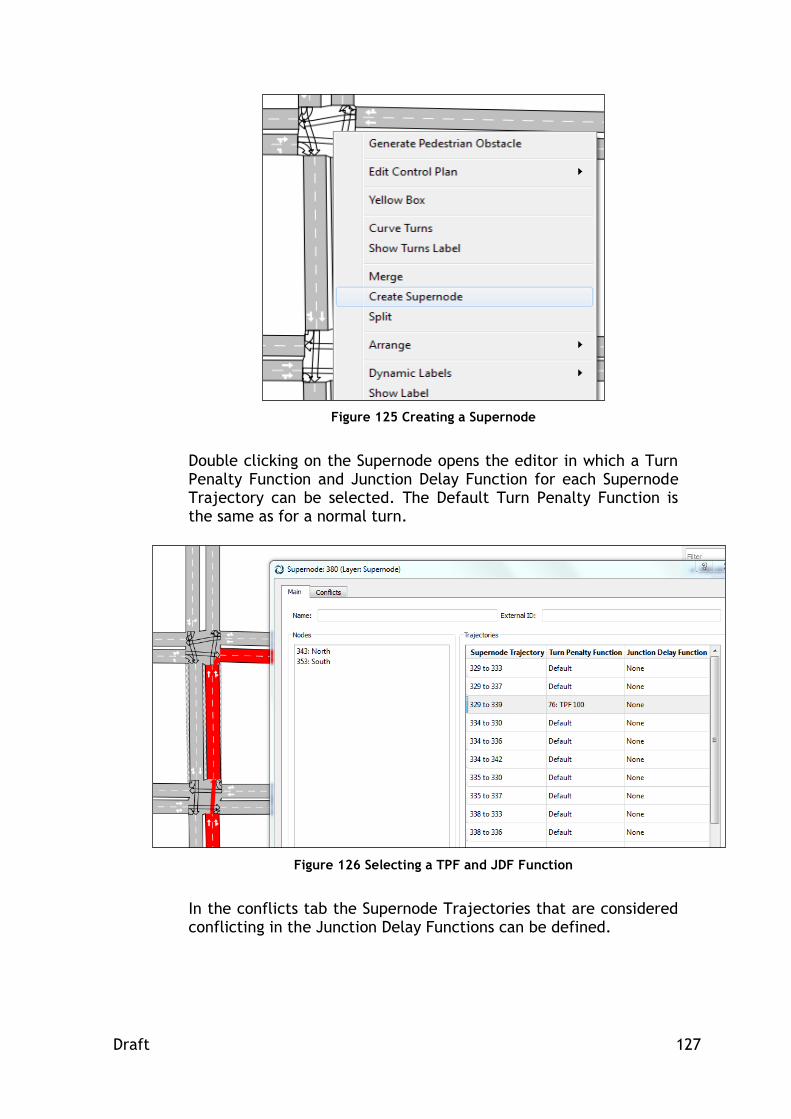
Draft 127
Figure 125 Creating a Supernode
Double clicking on the Supernode opens the editor in which a Turn Penalty Function and Junction Delay Function for each Supernode Trajectory can be selected. The Default Turn Penalty Function is the same as for a normal turn.
Figure 126 Selecting a TPF and JDF Function
In the conflicts tab the Supernode Trajectories that are considered conflicting in the Junction Delay Functions can be defined.

Draft 128
Figure 127 Defining Supernode Trajectory conflicts

Draft 129
13 Centroids and Centroids Configuration Editing
Centroids are origin and/or destination of trips in a transportation network when using O/D matrices. They can be connected to either sections or nodes. A connection is used to introduce flow in the network (a ‘To’ connection), in which case it is drawn in blue, or to extract flow from the network (a ‘From’ connection) in which case it is drawn in green. Centroids can be connected to more than one object. This means that the centroid will introduce and/or extract flow in/from more than one section or node. In this case, the user can decide how the flow is assigned to each connection by setting the usage percentage. A set of centroids are grouped in a centroids configuration.
13.1 Centroids Configuration
Aimsun allows multiple configurations in a network. This is useful to hold O/D matrices for the whole network and O/D matrices for sub areas of this global network. They can also be used to represent variations of demand due to future infrastructures (for example a new road or a new park and ride area). A centroids configuration holds a set of centroids and the related (to these centroids) O/D matrices and O/D routes. A centroid is in one, and only one, configuration.
13.1.1 Active Centroids Configuration
More than one configuration can exist in the same network but only one can be active (for editing) or in use (in a simulation for example) at the same time. Only centroids from the active configuration will be drawn. The active configuration is marked in the Project window with the
icon in blue colour. The rest of configurations are marked in
grey . A Centroids Configuration can be activated by right clicking on it in the Project window and choosing the Activate option. The previously active Centroids Configuration will automatically be deactivated.

Draft 130
Figure 128 Activating a Centroids Configuration
When the user creates a new centroid, it will be added to the active configuration.
13.1.2 Centroids Configuration Editing
A new centroids configuration can be created from the Project menu or using the Project Centroids Configuration folder’s context menu. The new configuration becomes the active one. Using its context menu, a centroids configuration can be deleted using the Remove command, it can be activated with the Activate command or renamed using the Rename command. It can also be renamed by selecting it and pressing the rename key (F2 by default). Centroids configurations can be duplicated using drag and drop (over the Centroids Configuration folder). This command will duplicate the configuration and all the centroids, O/D matrices and O/D routes in it.
13.2 Centroid Manipulation
Use the Centroid Tool to create new centroids. Select the tool and press over a 2D view to mark the position of the new created centroid.
Figure 129 Centroid Tool
A centroid can be moved (although changing its position will not change the point where the flow enters or leaves the network), renamed and duplicated (using Copy and Paste commands). A centroid represents a zone, an area in the network, and so for graphical visualisation it’s linked to a Polygon that can be edited from its context menu.

Draft 131
Figure 130 Editing the Centroid’s Polygon
The shape of the Polygon can be edited by the user, or the menu option Tools -> Centroid Tessellator can be used to calculate an automatic partition of the network:
Figure 131 Centroid Tessellator
13.3 Centroid Editor
Double click on the centroid to edit it. The user can, from its editor (see Figure 132), connect the centroid to sections and nodes using different settings. The editor also names the centroids configuration that holds the centroid and in which matrices (Trips folder) and routes (O/D Routes folder) it is used.

Draft 132
Figure 132 Centroid Editor
When a centroid is connected to more than one object to insert or attract traffic flow, it is possible to determine how these different connections will be used in the dynamic simulators. When set in Same Percentages to All, the usage percentage will be evenly shared by all the connections - no editing of the percentage is allowed. When Same Percentages to All is not set, the user must edit the usage percentage for each connection. The sum of percentages per type must be 100. Independently of the assigned percentage Aimsun is allowed to discard this data and put or get the flow from the more attractive connected object (as calculated by the Route Choice model). The attributes Use Origin Percentage and Use Destination Percentage control this behaviour. See the Aimsun Dynamic Simulators Manual for more information. The Use Best Entrance parameter sets whether the route choice algorithm will take into account, for each origin centroid and for each calculation, only the one shortest path from the entrance with the lowest cost (Use Best Entrance checked) or one shortest path from each entrance section (Use Best Entrance not checked).

Draft 133
With any of the connections selected in the table (click on the desired row, at the Object or ID column), pressing the Show Connection Attributes button will change the editor view to the connections information.
Figure 133 Connection Attributes editor
Press the Show All Connections to come back to the original view.
13.3.1 Connection Editing
Press the New button and then press on the section or node that will be connected to the centroid. A connection has the following attributes:
Type: To define if the vehicles will be generated to the object or attracted from the object where this centroid is connected to.
Percentage (Dynamic simulators): Whenever the Use Origin Percentage or Use Destination Percentage options are ticked, this parameter defines the percentage of vehicles to use this connection.
Vehicle Class (Dynamic simulators): A centroid connection can be used by specific vehicle types only. If that is the case, a vehicle class with the allowed vehicle types must be defined and selected here.
VDF (Macro): The Volume Delay Function that corresponds to this connection.
Select the connection in the editor to change any of the above parameters.

Draft 134
Select a connection and press the Delete button to remove a connection. Connections can also be created outside the editor using the Connection tool. Refer to the Connection Tool section for details.
13.3.2 Trips
In the Trips folder, the summarised information about the number of O/D pair trips defined in each matrix, where the edited centroid is origin or destination of the O/D pair, is shown. When an information line is clicked, the other centroid in the O/D pair is marked in the primary colour in the active 2D view. The total generation and attraction capacity of the centroid for every matrix is also shown.
Figure 134 Trips Folder
13.3.3 O/D Routes
In the O/D Routes folder, all the routes that start or end in the edited centroid are shown.

Draft 135
Figure 135 Routes Folder
When selecting any one of them, it is drawn in the 2D views using the primary colour. See the O/D Route Editing section for details on editing O/D Routes.

Draft 136
14 O/D Route Editing
An O/D route contains all the sections defining a path between an origin centroid and a destination centroid. Use the context menu of a Centroid Configuration to create a new O/D Route. Then, a new empty O/D route will be added to the O/D Routes folder inside the centroid configuration. These O/D Routes are afterwards accessible from the O/D matrices, so that the percentage of use of each of them can be defined. Refer to the Path Assignment section for details. O/D Routes are also listed in their origin and destination centroid editors. Refer to the O/D Routes section for details.
14.1 O/D Route Editor
The O/D Route editor can be opened by double-clicking on the O/D route in the Project Window (O/D Routes folder) or accessing to the Properties in its context menu. The O/D Route editor is used either to set the sections that will define the O/D route, to modify the O/D route, or simply display the O/D route.

Draft 137
Figure 136 O/D Route Editor
Once the editor is open, an O/D route is defined by clicking on the active 2D view the sections (in order) that will form the path. Some intermediate sections can be omitted as long as there is a unique path to go from the last specified section to the next one. The sections belonging to the O/D route when the O/D route editor is opened are drawn in the primary mark colour in the active 2D view.

Draft 138
15 Subnetwork Editing
A subnetwork is a subarea of the global network that can be analysed individually. Once the geometry for the area that needs to be analysed (without taking into account the rest of the network) has been created, the subnetwork can be defined. To do this, first create a polygon that encloses the area. Refer to the Polygon Graphical Editing section for details on creating a polygon. Once the polygon has been created, it can be converted to a Subnetwork right clicking on the polygon and selecting Convert To / Subnetwork. This can be shown in Figure 137.
Figure 137 Subnetwork Creation
The polygon shape will change to a red discontinuous line defining the border of the Subnetwork. Furthermore, a new subnetwork will be added to the Project Window -> Subnetworks folder, as shown in Figure 138.

Draft 139
Figure 138 Subnetwork Polygon and line in the Project Browser
The Subnetwork editor can be accessed either by double clicking on the subnetwork in the Project window or by double clicking on the subnetwork polygon (provided that the subnetwork layer allows edition, otherwise the subnetwork polygon is not selectable). The appearance of the polygon can be changed in the subnetwork editor, exactly as with regular polygons.
Figure 139 Subnetwork editor
If no information is entered in the editor’s Sections folder (that is, the default state), the part of the network within the polygon lines will belong to the subnetwork. A node is considered to belong to the Subnetwork if at least one of its turns is completely inside the polygon. A section belongs to the Subnetwork if at least the initial or ending point in its central line is inside the polygon or if any of its origin or destination nodes belongs to the Subnetwork. Another way to define a subnetwork is by the selection of a set of sections (for example, the highway part of a network).

Draft 140
Figure 140 Sections folder in the Subnetwork editor
Then, the list of sections must be specified in the Sections folder. Sections are selected directly in the view, and by pressing the Add Selection button, they will be added to the list. In this case, the subnetwork contains all the sections listed, plus all the nodes with any of its turns connecting sections in the list, plus the sections connected to the nodes belonging to the subnetwork. For example, if all the sections of road type highway are listed, the subnetwork will contain the highways as well as the on- and off-ramps As usual, by opening a subnetwork’s context menu (right click on the Subnetwork in the Project menu), the subnetwork can be renamed. Other commands available using the context menu (see Figure 141) are the creation of a centroids configuration for the subnetwork, a traffic state, a traffic demand and scenarios for an Aimsun Dynamic simulation or Macro Assignment or Adjustment or Travel Demand Modelling scenarios. All these objects have the same properties in a subnetwork as they have in the global network. Refer to their specific sections for details.
Figure 141 Subnetwork Context Menu

Draft 141
When creating the first subnetwork a new layer will be created named subnetworks into which all subnetwork polygons will be added, as shown in Figure 142.
Figure 142 Subnetworks Layer
If the existing subnetwork borders want to be protected from editing the corresponding layer parameter Allow Object Editing will need to be unchecked. By default, the subnetworks will be editable. In order to access the context menu of the Subnetwork, to access its editor by selection of the Subnetwork on the 2D View, or to add/remove/modify its vertices, this parameter must be checked. In 2D views, when no filter is selected the whole network is drawn. If only a subnetwork must be drawn in a 2D view, select it in the Filters option from the View context menu.

Draft 142
16 Non-Graphical Data Editing
All the non-graphical data (traffic demands, vehicle types, control plans, dynamic scenarios…) is located in the Project Browser and data items are created from: (i) the Project menu; (ii) the context menu on Project folders (for example, right clicking on the Vehicles folder, as shown in Figure 143, reveals a context menu where a new vehicle type or a new vehicle class may be created); or (iii) using the context menu of some objects (O/D matrices are created from, and placed into, a centroids configuration).
Figure 143 Right click on a project folder to access its context menu
From the Project Browser the user can edit (double click), rename (context menu), duplicate (drag and drop) and delete (context menu) this data. The Project Browser organizes related data into folders. The current version does not allow the free organization of the data into user-defined folders. The only possible customization is to change the name of these predefined folders.

Draft 143
There are several main folders where all the objects are organised. These folders and the objects that they contain are:
Scenarios: where the dynamic, macro and travel demand modelling scenarios will be located.
Network Attributes Overrides: where the Network Attributes’ Overrides can be set.
Demand data: where the centroid configurations, generation/attraction areas, distribution areas, parking areas, generation/attraction data set and data set attributes, the distribution data set, the traffic states, the traffic demands, the traffic arrivals, the time periods, the transportation modes, the initial states, the functions, the macro function components, the traffic profiles, the vehicle types, the vehicle classes, the trip purposes and the user classes will be located.
Control: where the control plans and master control plans will be located.
Public Transport: where the public transport lines, public transport plans and public transport stations will be located.
Infrastructure: where the road types, the lane types, subpaths and the optimal detector locations analysis (if the Aimsun macro is loaded) will be listed.
Traffic Management: where all the traffic management objects will be listed.
Data Analysis: where the view modes, view styles, real data sets and grouping categories will be listed.
Subnetworks: where all the different subnetworks defined for the global network will be listed.
Scripts: where all the existing python scripts will be listed.

Draft 144
17 User Classes, Transportation Modes, Trip Purposes, Vehicle Types and Vehicle Classes Editing
These five concepts are found in the Demand Data Folder, in the Project window. Use the Project menu or the Demand Data context menu to create a new User Class, Transportation Mode, Trip Purpose, Vehicle Type or Vehicle Class. They can also be created from their own folder context menu (User Classes, Trip Purposes, Transportation Modes and Vehicles, the last one containing both Vehicle Types and Vehicle Classes).
Figure 144 User Classes, Vehicles, Transportation Modes and Trip Purposes folders
17.1 Vehicle Type Editor
The vehicle type editor is used to specify the physical characteristics and the models’ parameters of a type of vehicle. In the Main folder, the vehicle type’s Name and External ID can be defined.
Also the vehicle type’s main parameters such as Length, Width and Maximum Desired Speed can be defined. They are:
Length: Mean, deviation, maximum and minimum values.
The length, in meters or feet, for this type of vehicle. This
parameter is used both for graphical and modelling purposes.
It has a direct influence on traffic modelling, as vehicle
length is taken into account in all vehicle behaviour models.

Draft 145
Width: Mean, deviation, maximum and minimum values. This
is the width, in meters or feet, for this type of vehicle. This
parameter is only used for graphical purposes and does not
have a direct influence on the traffic modelling.
Maximum desired speed: Mean, deviation, maximum and
minimum values.
This is the maximum speed, in km/h or miles/h, that this
type of vehicle can travel at any point in the network.
For example, one could define a ‘sports car’ vehicle type
with a mean desired speed of 110 km/h, a deviation of 10
km/h, a maximum value of 140 km/h and a minimum value
of 90 km/h. Sports cars would be sampled from a Normal
(110,10) distribution.
To edit any of these values, click on the desired cell and type the new value. These three parameters are defined using a mean value, deviation, minimum and maximum value. When generating a vehicle belonging to this vehicle type, the value for this parameter will follow a normal distribution based on the values edited. Please refer to the Aimsun Dynamic Simulators manual for more information about it.
The Maximum Capacity denotes the maximum number of passengers that can travel inside a vehicle of this vehicle type. This value can be set either as a multiplying factor of vehicle length or as a total value. This parameter is used by the Legion for Aimsun module when loading pedestrians into public transport vehicles and also in the Public Transport Assignment. Please refer to the Aimsun Dynamic Simulators manual or the Aimsun Travel Demand Modelling Manual for more information about it. To set the vehicle as articulated and to define the articulated parts, the Articulated folder must be used. Check the Articulated button to set the vehicle as articulated. Add new articulated parts by clicking on the Add button. Remove any undesired articulated part by selecting it on the list and clicking on the Delete button. In this folder the doors of the vehicle are also specified. This information will only be used in Public Transport vehicles when simulating pedestrians with Legion. See Aimsun Dynamic Simulators manual for details on Legion for Aimsun.

Draft 146
Figure 145 Vehicle Type Editor’s Main Folder
In the Dynamic Models and Microscopic Model folders the parameters used by the dynamic simulators are defined. They are mainly parameters such as the deceleration, giveway times, pollutant emission and fuel consumption, 2D and 3D visualization shapes, vehicle classes and default dynamic experiment parameters. Please refer to the Aimsun Dynamic Simulators Manual for more information about them. In the Static Models folder, two parameters are defined: Transportation Mode and PCUs. A Vehicle Type can belong to a Transportation Mode (for example, Car can belong to Mode Private). This information is used when modelling the Travel Demand with the Four-step Model. Please refer to the Aimsun Travel Demand Modelling Manual for more details on Transportation Modes and their usage. The PCUs parameter (Passenger Car Unit) is a measure of the space a Type of Vehicle needs compared to a passenger car. That is, the private car is considered as the unit, 1 PCU, and the rest of vehicles are converted to this unit by a factor.
17.2 Vehicle classes
The concept vehicle class is not associated with the physical characteristics of each type of vehicle (e.g., cars, buses, and trucks), but rather with the use of the network that vehicles make. Examples include private vehicles, public vehicles, and emergency vehicles. This is used later to specify for which sort of vehicles a reserved lane is defined. For example, a ‘bus’ vehicle type can

Draft 147
have selective authorisation in some lanes because it belongs to the ‘public transport’ class. A vehicle type can belong to several vehicle classes. For example, a ‘guided taxi’ type can belong to the ‘public transport’ and ‘guided’ classes. The process of defining a class begins by selecting the New…Demand Data… Vehicle Class in the Project menu or in the Project window either in the Demand data or in the Vehicles folders’ context menu. This action will add a new Vehicle Class in the Vehicles folder in the Project window. Use the Rename option in its context menu to rename it. To set a vehicle type as a member of a vehicle class, the vehicle type editor must be used. See the Vehicle Type Editor section for details.
17.3 Transportation Modes
Transportation Modes are used for the Travel Demand Modelling. Every Vehicle Type (and thus, every User Class) can belong to only one Transportation Mode.
17.4 Trip Purposes
If there is information on Trip Purposes, they can be listed and then used to constitute a User Class pairing it with a Vehicle Type. This allows having trip matrices for different trip purposes and also assign them considering different generalized costs. No extra information is contained in the Trip Purpose editor, apart from its Name and External ID.
17.5 User classes
A User Class in Aimsun is the pair formed by a Vehicle Type + Trip Purpose. In a User Class, setting the Vehicle Type is mandatory, but not the Trip Purpose. When no information on the Trip Purpose is available and therefore no specific trip purpose is set, the user-class considered will be the pair VehicleType–Any (for example Car-Any, we specify the vehicle type but not the trip purpose). Also, when setting the Vehicle Type + Trip Purpose in the matrix editor, if the combination does not exist yet as a User Class, it will be automatically created. There can only be a unique User Class for each Vehicle Type + Trip Purpose combination.

Draft 148
Figure 146 User Class editor
Each Vehicle Type can belong only to one Transportation Mode (see Vehicle Type Editor section for more info) and consequently, a User Class will be related with only on Transportation Mode, which is listed in the editor (non-editable).

Draft 149
18 Traffic Demand
18.1 Editing Order
The order for editing traffic demand data is:
Create and edit the vehicle types to be used.
Create and edit the Origin/Destination matrices or the Traffic States that will be used for each vehicle type and time interval.
Create a new Traffic Demand and assign the O/D matrices or the Traffic States that will compose it.
Also before Aimsun Macro, Meso, Hybrid or Micro simulations are used we have to:
Assign the traffic demand to a scenario.
If required, assign values to variables in the scenario or in the experiments.
18.2 O/D Matrix Editing
An O/D matrix contains all the trips that will be generated in a network for a particular vehicle type and in a defined time period. The cell (i,j) of an O/D matrix contains the number of vehicles going from centroid i to centroid j. Matrices with other kind of contents (cost, travel times, distances, etc.) can be also defined in Aimsun, their edition is completely the same regardless of the type of contents of the matrix. Use the context menu of a Centroid Configuration to create a new O/D matrix for it. The Centroid configurations folder is located inside the Demand data in the Project window or inside the subnetwork folder if the centroid configuration belongs to a subnetwork. For every new O/D matrix, its name will be assigned following the structure ‘matrix vehType: initialTime duration’ (for example, ‘matrix car: 08:00 01:00’). When any of these parameters changes, the name will be automatically updated, unless the user edits the matrix name, in which case the automatic update will be cancelled. The auto naming will be activated again if the user introduces a void name, as it is compulsory for a matrix to have a name.
18.2.1 O/D Matrix Editor
18.2.1.1 Main
In the Main folder, the user will specify the vehicle type to be used and the time interval to which the data belongs. This information is compulsory for later assignments/simulations. Optionally, the user can specify the Trip Purpose and the Contents (what kind of data the matrix contains: trips, travel times, distances, etc.). In order to

Draft 150
define a Traffic Demand, the contents of the matrices should be trips, but other kind of contents can be used for other meanings (like skim matrices containing costs). The pair formed by a Vehicle Type + Trip Purpose constitutes a User Class in Aimsun (see section 17.5 User classes).
Figure 147 O/D Matrix editor – Main folder
Also in the Main window, we can see a Summary of the matrix data, with the number of Origins and Destinations, the Total value of the matrix (adding all the cells up), the Minimum (different than zero) and Maximum Value, and the number of Empty and Non Empty cells. Finally, the Store Location info is also available in this folder. Regarding to the O/D matrix storage, it can be stored in the Aimsun file, in an external text file or in the project outputs database defined in the Project Properties. Storing an O/D matrix in Aimsun means that the O/D matrix information will be stored in the Aimsun file (the .ang file). For big networks or even when working with networks where the matrix information can be shared among different software packages, storing the O/D matrix outside the Aimsun file can be useful. When storing an O/D matrix in an external ASCII file, the file path, the field separator to be used (tabulation or comma) and the parameter used as ID for identifying the centroids in the ASCII file must be defined (see Figure 148). For all the centroids, the stored ID used can be the ID used in Aimsun, the External ID, or the Name.

Draft 151
Figure 148 Parameters folder - Storing as ASCII file
The format of the ASCII file is the same one that is explained in the Copy and Paste Matrix Options section e.g. the format can be of Aimsun, Visum, Saturn or Emme. Only the centroids' IDs and the trips information are stored in the ASCII file. If the storing type chosen is the project outputs database, the parameter used as the identifier must be defined (see Figure 149). This ID, Name or external ID will be used to identify the centroids and the O/D matrix itself.
Figure 149 Parameters folder – Storing in a database
The data source, the username and password (these last two parameters may be omitted, depending as to whether the database requires them or not) are defined in the menu Project / Properties, in the main tab folder (see Figure 150).

Draft 152
Figure 150 Project Properties Editor – Setting the Outputs Data Source
The information stored in the database will be the O/D matrix From Time, its duration, all the trips, and the context information (that is, weekday, season, weather and event). When the storing type chosen is not the Aimsun file, that is, for both external ASCII files and database, only data about the matrix data location will be stored in the Aimsun file. When the Aimsun file is opened again, it will automatically retrieve the matrix if the external file is found or it will ask for the new location otherwise. In any case, while the network is open, the matrix information can be reread at any moment by using the Retrieve button. The Store button is used to store the current matrix information in the external file whenever it is pressed. If the Store Matrix is checked then whenever the Aimsun model is saved the O/D matrix information will also be stored in the external file.
18.2.1.2 Cells
In the Cells tab folder, the number of trips (or any applicable data) from each origin to each destination is listed/edited. During the editing of a cell, if the centroid configuration to which the matrix belongs is active, the origin (in rows) and the destination (in columns) centroids will be marked in the active 2D view. The primary mark colour will be used for the origin and the secondary mark colour for the destination.

Draft 153
The combo box to the top right of the editor, entitled Headers, allows the specification of which centroid attribute should be shown as row/column headers for the matrix, choosing among: “ID”, “External ID”, “Name”, or combinations of these. Columns and rows are ordered automatically based on these headers.
Figure 151 O/D Matrix Editor – Editing trips from one centroid to another
Any Centroid Grouping Category can be selected in the Grouping combo, in order to reduce the dimensions of the matrix while visualizing it. All cells in the same grouping will be either added or averaged depending on the Matrix Contents. For contents: Not Set, Trips, Parking Slots, Distribution: Through Traffic and Individuals, the sum is calculated for the aggregated cells, and for contents: Costs, Travel Times, Distances, Tolls, Speed and Ratio, the average (not weighted) is calculated. For Distribution: Blocked Cells, if one of the cells is Blocked, the cell aggregated by Grouping Category will also appear as Blocked. The Allow Negative Values checkbox allows to have a negative value in a cell when checked. For the user’s convenience, when the checkbox Execute Operations with Current Cell Value is active, a shortcut to add, subtract, multiply or divide by a constant value (also available with Add and Multiply operations) can be used by first selecting the desired cell, then typing the desired operation (for example: +4) and then pressing the Enter key. If no operation but a single value is written (for example: 100), after pressing Enter, the selected cell will be filled in with this value.

Draft 154
By default, only centroids with entrance connections will be listed as origin centroids and only centroids with exit connections will be listed as destination centroids. To list all the centroids as origin and destination without considering their current connections the Show All Centroids checkbox needs to be checked.
18.2.1.3 Operations
The operations, available from a combo box in the same editor, are:
Join: to add another matrix to this one. This command modifies the original matrix. The join types are:
o Concatenate: Sums the trip values of both matrices and sums the time durations.
Figure 152 Joining two O/D matrices as Concatenate
o Add: Sums the trip values but the duration of the original matrix is not modified. The duration of the second matrix is not taken into account
Figure 153 Joining two O/D matrices as Sum
Split: Creates N new matrices dividing the number of trips among the new matrices (see Figure 154). This command doesn’t modify the original matrix.
Figure 154 Split of trips in two matrices
A: 100 Trips-Vehicles
A 82%: 82 Trips-Cars
A 18%: 18 Trips-Trucks
9:00
10:00
11:00
A: 100 Trips B: 100 Trips
A + B: 200 Trips
9:00
10:00
11:00
A: 100 Trips B: 100 Trips A join B: 200 Trips
9:00
10:00
11:00

Draft 155
If the option Split Duration is activated, the new matrices will have an initial time and duration automatically calculated to cover, as time intervals, the one from the original matrix. The duration will be splitted proportionally to the number of new matrices, not to their percentage.
Figure 155 Split of trips and duration in two matrices
If the option Automatic Factor is activated, then the percentages will be distributed uniformly among all the new matrices specified.
Add: Adds trips to the cells of the matrix, either to all the cells of the matrix, to a selection of cells or by a condition. The option Apply to Empty Cells allows adding trips to the empty cells. When the option is not activated, the trips will be added to the cells with defined trips only (i.e., with a number of trips greater than 0).
Figure 156 Add operation
Multiply: Multiplies the trips in the matrix by a factor, either for the entire matrix, for a selection of cells or by a condition.
Transpose: Transposes the matrix or part of it.
Furness: Balances the matrix taking into account new generation or attraction values in some centroids. See Aimsun Macroscopic Modelling Manual for more details on this operation.
Filter: Does a filtering action (hide or highlight) on the cells of the matrix that match the comparison condition given.
Classify: Colours the cells of the matrix according to a range of values. These ranges can be calculated automatically or specified by the user.
Redistribute: An O/D matrix has a specific cost distribution based on any of its corresponding skim matrices (for example,
A: 100 Trips
A 50%: 50 Trips
A 50%: 50 Trips
9:00
10:00
11:00

Draft 156
the O/D distances matrix). After an adjustment, this distribution might have been distorted, and it can be recovered by executing a Redistribute operation that will need the following as input: the matrix to be redistributed; its current corresponding skim matrix; the original demand matrix; the original skim matrix (these last two giving the cost distribution that you want to recover).
Correction: This operation will apply the same (multiplicative) changes to the current matrix that were made from an original matrix to a manipulated matrix (for example, an adjusted matrix) up to a maximum correction factor.
Cell-by-Cell Operations: adds, substracts, multiplies or divides the cell values of the current matrix by the cell values in the specified matrix.
Apply Traffic Profiles: This operation will apply the traffic profiles selected per cell, obtaining O/D matrices for each interval in the profile and with values multiplied by the percentage stated in the profile.
18.2.1.4 Histogram
In this folder, a histogram based on the cell values is available. The user can choose the number of intervals, and edit the ranges. The Units can be number of Vehicles, or PCUs or any of these two in percentages. Also, the Empty Cells (with a zero value) can be included or not in the plot. By selecting a secondary matrix, the histogram will be calculated by weighting each cell by the corresponding cell in the secondary matrix (for example, a distance matrix weighted by the number of trips).

Draft 157
Figure 157 Matrix Histogram
18.2.1.5 Path Assignment
In this folder, the percentage of use of the paths previously defined as well as the percentage for the ICSP (Initial Calculated Shortest Path) between a pair of O/D centroids can be assigned, so that these values are taken into account for Dynamic simulations. To do so, select an origin and a destination centroid (or list all of them by selecting All). Then, all the paths defined for this O/D pair will be listed. If it does not have any user-defined path, then only its corresponding ICSP will be shown. The percentage of use of each path in the current matrix can be set here. The total sum of the percentages for each O/D pair and cannot be higher than 100. Figure 158 shows how to set 65% of cars travelling from centroid SE to centroid NE to use a user-defined path. The remaining 35% of cars will choose among that path or other alternative paths according to the active route choice function.

Draft 158
Figure 158 Stochastic Path Assignment
In this folder, there is also a button to set the same percentage for all the ICSP (Initial Calculated Shortest Paths). To do this, click on the Set Common ICSP Percentage button. A new dialog will appear in which the new ICSP percentage for all the O/D Pairs may be defined.
Figure 159 Dialog to set the ICSP Percentage for all the O/D Pairs
18.2.1.6 Parameters
The editor has also a Parameters tab folder to define context data to classify the O/D matrix. This context data is not used by the simulator but can be relevant for other functionalities. The user can store information about the day of the week, weather, season, event and methodology used to calculate the O/D matrix.

Draft 159
Figure 160 Parameters Folder
18.2.1.7 Copy and Paste Matrix Options
The O/D matrix editor allows the interchange of data with other software using the copy and paste command. To copy an O/D matrix or a selection of the cells from Aimsun to any other software, select the desired cells and either click the Copy button or press CTRL+C. The selection will be copied together with its ID context, that is, the ID heading, and the centroid ID for each row and column. When no cell is selected, the copy operation will copy the whole matrix. There are two possibilities to paste information into an O/D matrix: with or without context. When pasting without context, the paste data will be copied exactly starting at the currently selected cell in the O/D matrix.
Figure 161 Structure of an O/D matrix with context

Draft 160
There are three types of context, which must be specified in the source table:
‘id’: the centroids ID will be used to locate a cell.
‘name’: the centroids name will be used to locate a cell.
‘eid’: the centroids external ID will be used to locate a cell. If the paste includes a context, the context type must be specified in the heading (as in Figure 161 bordered in blue in Figure 162). In this case, the cell that is currently selected in the editor is not important and neither the order of the rows and columns: as each cell is correctly identified by the context, the paste will automatically fill the corresponding cells.
Figure 162 Result of the paste operation in an O/D matrix
18.2.1.8 Duplicate Matrix
The Duplicate button, in the bottom part of the matrix editor, can be used to create a new matrix in the same centroid configuration with the exact same data as the matrix that is being duplicated.
18.3 Traffic States editing
A traffic state contains all the input flows that will be generated in a network for a particular vehicle type and a defined time period as well as the turn proportions at nodes (when more than one turn is possible from a section).

Draft 161
Traffic States can be only used in Aimsun Dynamic Simulators, that is Micro, Meso or Hybrid but not in Aimsun Macro. Aimsun Macro requires O/D matrices. Use the New…/ Demand data / Traffic State option in the Project menu, the Demand Data folder’s context menu or the Traffic States folder’s context menu of the Project Window to create a new Traffic State. For every new Traffic State, its name will be assigned following the structure ‘state vehType: initialTime duration’ (for example, ‘state car: 08:00 01:00’). When any of these parameters changes, the name will be automatically updated, unless the user edits the traffic state name, in which case the automatic update will be cancelled. The auto naming will be activated again if the user introduces a void name, as it is compulsory for a state to have a name.
18.3.1 Traffic state editor
The traffic state editor is used to define all the traffic state’s properties. Open it by double clicking on the desired traffic state in the Project Window.
Figure 163 Input Folder
In the Input Flow folder, the vehicle type, the initial time and the duration of the traffic state can be defined. In addition, the flows entering each section can be specified. All the sections in the network or only the ones that are entrance points to the network

Draft 162
can be shown. Note that the Aimsun Micro Simulator will not take into account the input flows defined in the intermediate sections. Finally, a percentage (value between 0 and 100) of flow that will be kept in a section, that is, will enter the section but not exit it, can also be defined. Note that the Aimsun Simulator will not take into account this value. When defining the input flows, there is the possibility to do it taking into account the input turns, that is, distinguishing among the previous sections, or not. To do this, select, in this editor, the desired section where to select among its entrances and press the Use Input Turns button. One line for each section entrance will appear. In the Turn Info folder, all the turn percentages from a section to all the sections accessible from it can be defined. This folder can show all the sections or only sections where the percentages are relevant, that is, sections with more than one turn. Similar to the previous folder, the turn percentage can take into account where the flow into the current section came from. If the flow’s preceding section must be taken into account, select the section, in the editor, and press the Use Input Turns button, if not, select the section and press again in the Don’t Use Input Turns button.
Figure 164 Traffic State Editor – Turns Info folder
The user can also define exit flows instead of turn percentages when these values are available. If the exit flows are specified, then the turn percentages can be automatically calculated using

Draft 163
the Recalculate Turn Percentage using Exit Flows button. Note that the Aimsun Micro simulator will not take into account the turn flows defined. It will use the turn percentages. For example, when a traffic state is created using the flow information of a static traffic assignment (done with the Aimsun Macro) both the turn percentages and the turn flows are known. The Highlight wrong definitions checkbox activates colouring on the first column of the table. The cells will remain “uncoloured” when the turn percentages are correctly defined; they will be painted in red when the sum of the turn percentages coming from a section is not equal to 100; and will be painted in orange when no value is entered in the table for all the turns coming from a same section. This orange highlighting does not necessarily mean the definition is wrong, but it will be interpreted as if 100% of flow was assigned to the first turn and 0% to the remaining turns. Finally, in this editor, as in the O/D matrix editor, values can be copied into or pasted from an external spreadsheet application using the Copy/Paste buttons, and some parameters such as the day of the week, weather, season, event and methodology used to calculate the traffic state can be set.
18.4 Traffic Demand
In Aimsun, both the Traffic States and the O/D matrices are for a unique vehicle type (plus trip purpose in the case of O/D matrices, that is, for a unique user class) and for a unique time interval. For example, an O/D matrix for the vehicle “car”, trip purpose “Any” that starts at 8:00 AM and has a duration of 1 hour. Several O/D matrices or Traffic States (but not a mixture of both) will be grouped into a Traffic Demand. A Traffic Demand thus contains traffic data for several vehicles (or several user classes) and time intervals and can be used, for example, as input for an Aimsun scenario (either static or dynamic).
Figure 165 A Traffic Demand for three vehicle types
A traffic demand can be created by accessing the New…/ Demand Data / Traffic Demand command either in the Project Menu, the Demand Data folder’s context menu in the Project Window or in
Cars, O/D 1
Trucks, O/D 2 Trucks, O/D 3
9:00
10:00
11:00
HOV, O/D 4

Draft 164
the Traffic Demand folder’s context menu. Once done, a new traffic demand will be added to the Traffic Demands folder in the Project Window.
18.4.1 Traffic demand Editor
Open the traffic demand editor by double clicking on the desired traffic demand in the Project Window.
Figure 166 Traffic Demand Editor
In this editor, the user can select whether the traffic demand will be composed of matrices or traffic states. The time interval where this traffic demand will be applicable can be defined modifying the Initial Time and Duration. To add a demand item, that is, either an O/D matrix or a Traffic State, the Add Demand Item button must be pressed. When pressed, a list of all the O/D matrices grouped by Centroid Configurations or all the Traffic states will be shown from which the user can select the desired one. If the user chooses matrices, by checking any of the Centroid Configurations all of its O/D matrices are selected. User can also select single items or even all of them by checking Select All.

Draft 165
Figure 167 Traffic Demand Editor – Select objects of type O/D matrix
Once selected, the item will be added to the Gantt diagram. Click on the item in the Gantt diagram to select it. Once selected, it can be scaled and moved to fit in the desired interval.
Figure 168 Gantt Editor
Press the Add Demand Item and repeat all the steps as many times as demand items must be added. As the traffic demand items are defined for a single vehicle type, there will be a line in the Gantt Diagram for every vehicle type selected in the added items. To remove an item, just select it in the Gantt diagram and press the Remove Demand Item button. The editor also offers the possibility to modify the initial time and duration of an item without moving or scaling it in the Gantt diagram but by typing times in the Demand Item properties folder once it is selected.
Figure 169 Demand Item properties
NOTE: when using O/D Matrices, the duration defined for each demand item in the Traffic Demand will be the duration used to enter all the trips defined in the O/D matrix. Therefore, if the user has defined an O/D matrix of 6000 trips from A to B with duration

Draft 166
of 2 hours, and the demand item is defined for one hour, then Aimsun Dynamic simulators will try to put 6000 vehicles in one hour. The user can change the Factor to multiply any O/D matrix or Traffic State by a factor to increase or decrease the flow or number of trips without modifying the item itself. There is also a global factor that affects all the traffic demand items in a traffic demand. These factors can be a percentage or a variable. If it’s a percentage, the user can set 100 % to use all the trips, 50 % to use half the trips, 120 % to generate 20 % more trips than the number found in the O/D matrix or traffic state, and so on. If it is a variable, the percentage value to be used (100 %, 120 %, 80 %,...) will be set at the scenario or the experiment level. Look in the Aimsun Dynamic Simulators Manual for more information about defining variables. When the traffic demand is based on O/D Matrices, a Traffic Arrivals object can be also specified. This object is generated and can be used in a dynamic simulation. Look in the Aimsun Dynamic Simulators Manual for more information about defining and using traffic arrivals. The traffic demand includes also a Summary with the total number of trips per O/D pair for each user class. Note that the summary doesn’t take into account factors defined as variables (as the final value depends on the chosen scenario).
Figure 170 Traffic Demand summary showing trips for the car vehicle type

Draft 167
The Profile folder shows the demand profile, that is, a diagram showing the total number of trips of each of the matrices in the demand, for each user class.
Figure 171 Traffic Demand profile

Draft 168
19 Control Plans
A control plan specifies the control parameters applied to each junction and metering in a network.
19.1 Editing Order
The editing order for control plan data is:
Create and edit the Control Plans that will be used.
Create a new Master Control Plan and assign the Control Plans that will compose it.
When Aimsun Micro, Aimsun Meso or Aimsun Hybrid are going to be used:
Assign the master control plan to a scenario.
19.2 Control Plan Editing
To create a new control plan select the New…/ Control / Control Plan option either in the Project Menu, in the Project Window Control folder’s context menu or in the Project Window Control Plan folder’s context menu. Once done, the new control plan will be added inside the Control Plans folder in the Project Window.
19.2.1 Control Plan editor
Open the control plan editor by double-clicking on the desired control plan in the Project Window.
Figure 172 Control plan editor

Draft 169
In this editor, the control plan can be renamed. Use also the Rename option in the Control Plan’s context menu to rename it. The Initial Time at which this control plan was designed to start at can be defined here. It is the absolute time at which the nodes' group of phases will be set at time 0. This parameter was known as Offset in previous versions. The Initial Time doesn’t have to match the time at which the Control Plan will be set to start in the Master Control Plan. The Control Plan will be applied in any case taking into account its Initial Time. So, for example, if the Initial Time is set to 00:00:00, the cycle on one node is 90 seconds and the Master Control Plan states that the Control Plan is applied from 08:00:00, then at 08:00:00 the Control Plan in that node will be at second 30 of the cycle. A list with all the nodes in the network and the control type associated to each of them is shown. When the control information has not been specified in a node, the control type is set to Unspecified. Otherwise, the control can be uncontrolled, fixed, external or actuated. To specify the control information in a node, double-click on the desired node in this editor’s node list or right-click on the node in any 2D view and select Edit Control Plan and the desired control plan. The Control Plan editor for the node will open. A list with all the meterings in the network and the control type associated to each of them is also shown. As it happens with nodes, when the control information has not been specified in a metering, the control type is set to Unspecified. Otherwise, the control can be uncontrolled, fixed, or external. To specify the control information in a metering double-click on the desired metering in this editor’s metering list or right-click on the metering itself in any 2D view and select Edit Control Plan and the desired control plan.
19.2.2 Control Plan Editor for Nodes
Use the node context menu to open the editor for the chosen control plan. If there is not a control plan, you can create a new one from this menu.

Draft 170
Figure 173 Node context menu
You can also use the control plan editor, from the Project window, to select the node to edit as previously discussed.
Figure 174 - Control editor for a node
Five different node types are available:
Uncontrolled: node managed by stops and give-ways. The traffic lights, if any, are disconnected.
Fixed (or pre-timed): node managed by traffic lights with fixed green-light phases. Different control plans may be assigned to different time periods, to simulate the change of timings depending on the time of day.
Actuated: Traffic control system that follows the NEMA (National Electrical Manufacturers Association) standards. For further details on those standards, please refer to NEMA

Draft 171
Standards Publication TS 2-2003 v02.06 Traffic Controller Assemblies with NTCIP Requirements.
External: It follows pre-timed control but can be combined with an external control policy implemented using the Aimsun Microsimulator API Extensions.
Unspecified: node without any control plan information defined. This type is used when working with different zones to let the simulator know that the control plan for the previous zone is still in use.
The Offset parameter is used to synchronise adjacent nodes (green wave). It formally specifies the displacement that is applied to the node's cycle when the control plan is initialised (e.g., an offset of –3 means that 0 seconds after the beginning of the control plan, the state of the traffic lights at this node will be the ones defined for second 3 in the node's control plan). The specified Yellow time is not inserted between one phase and the next but it replaces the initial seconds of the red phase. Consequently, if for a certain turn movement its green phase is assigned 34 seconds and the rest of the cycle lasts 66 seconds, then setting a 4 second yellow time will model that traffic light as 34 seconds of green light plus 4 seconds of yellow plus 62 seconds of red light. The behaviour of vehicles under yellow light has two phases depending on the red percentage defined, that indicates the percentage of yellow time the vehicles will consider as red. The first phase is the percentage of the yellow time (i.e. 3 seconds in case of a 4 seconds yellow time with a red percentage of 25%) when the drivers consider that yellow time is basically the same as green time. During the rest of the yellow time (i.e. 1 second in case of a 4 seconds yellow time with a red percentage of 25%), the vehicles apply a normal braking rate, instead of the maximum one they could reach under red light. The yellow time defined for the node can be overwritten at the level phase specifying a different yellow time for the desired phase. The yellow time at the phase applies to movements becoming red at the beginning of the phase. Then, for example, a yellow time on an interphase will apply to the movements that were green in the previous phase and that turn to red in the interphase. The Rest in Red parameter is only necessary for actuated control and consequently it will only appear when the control type is
Red percentage
Figure 175 - Red percentage modelling of the yellow time

Draft 172
defined as Actuated. For further details on the Actuated and Detectors folders please refer to Aimsun Dynamic Simulators User’s Manual. When the type is external, there is a critical check option used to mark those nodes that may have a preferential treatment in a given external adaptive system. This parameter is only considered when the simulator is plugged to an external adaptive control system that requires it as input. Clicking the button where the cycle length is shown opens a dialog where the cycle duration is defined in seconds.
19.2.2.1 Timing folder
In the Timing folder, the different phases of the intersection cycle are defined. A phase is defined as a time period for which there are no changes in the state of the traffic lights at that node. The timing defined can be viewed as Phases or as Signal Groups. When viewed as Phases, in the Gantt diagram the different phases defined are drawn. When viewed as Signal Groups, the phases visualization will change to a signals visualization where the green and yellow times for each signal can be seen. Phases are built in the following way: first the phase is created by clicking on the Add Phase button; then it is modified by adapting it in the Gantt diagram to its desired start time and duration and finally selecting the signal groups (each active signal group enables its associated turns) as being active (green) during that phase. When making a phase longer by dragging its border, the neighbouring phase is shrunk if necessary. If the drag is to the right, and the [Ctrl] key is pressed the cycle time will grow instead, maintaining the duration of the following phase. The signal groups are listed in the Basics subfolder and they are selected by ticking the Assigned to Phase column on the desired signal group. The Flash in Green column is merely used for display purposes and ticking it means the signal group will flash in yellow during its green time instead of being drawn in green. The Interphase parameter located in the Basics subfolder is an optional type of phase to model the fixed clearance time in between phases. This type of phase is then set between phases. For instance, an intersection with a 60-second cycle and two equally important movements (symmetric distribution of time), could be modelled with:
2 phases
2 interphases (each interphase in between the two phases)
24 second phases and 6 second interphases

Draft 173
3 second yellow time (either at the global level for the node or at the interphases)
This would produce 24 seconds of green light, 3 seconds of yellow light and 3 seconds of clearance time plus 30 additional seconds of red light (that is a total of 33 seconds of red light) for each one of the movements. In Fixed Controls, a Minimum Duration field, taken into account for Preemption, will be shown. Refer to the Aimsun Dynamic Simulators User’s Manual for further information. For External Control, the Minimum Duration and Maximum Duration fields are available. Finally, the yellow time for each phase can be defined as a global one defined for the node or as a different value specific for the movements changing to red at the beginning of the phase being edited. When a phase is selected, the allowed turns, that is, the turns associated with the active signal groups, are drawn in the active 2D view in the primary mark colour. When the Control type has been set to Fixed and the timing is set to be viewed as Signal Groups, it enables a different way of defining the control plan. This method bypasses the need to define Phases and consists of defining Start Time and Duration for each signal group. The buttons Add Signal Column and Remove Signal Column can be used to add or remove a pair of columns from the end of the table so more than one Start Time-Duration pair can be inserted per signal group. When the Control type has been set to Actuated or External, a Minimum and Maximum Duration for each phase can also be specified. For further details on the Actuated and Detectors folders please refer to Aimsun Dynamic Simulators User’s Manual or to NEMA Standards Publication TS 2-2003 v02.06 Traffic Controller Assemblies with NTCIP Requirements.

Draft 174
Figure 176 Editing a Control Plan using Signal Start Time and Duration
19.2.2.2 Pre-emption folder
The pre-emption folder is an editing window for the different pre-emption strategies, which lines to attend, the nature of the service and which detector will trigger the service. For further details on the Pre-emption folder, please refer to the Aimsun Dynamic Simulators User’s Manual.
19.2.3 Control Plan Editor for Meterings
Use the metering context menu to open the editor for the chosen control plan. If there is not a control plan, you can create a new one from this menu.

Draft 175
Figure 177 - Metering context menu
You can also use the control plan editor, from the Project window, to select the metering to edit as previously discussed.
Figure 178 - Metering Control folder
The control type policies associated to the metering can be:
Unspecified: when no control editing has been made.
Uncontrolled: when the metering device is assumed to be disconnected.
Fixed: when a fixed criterion for allowing flow to go through is used. That means that none of the parameters of the metering will vary in time for this control.
External: the parameters initially set can vary between a given maximum and minimum depending on traffic conditions and according to an external user-set algorithm (using the Aimsun Micro API).

Draft 176
Depending on the metering type, different parameters need to be defined:
For green time meterings, the user must set the cycle’s total time (that is, the time of green plus the time of red), the offset of the first green time related to the initial time of the control plan, the time of green,, the yellow time, flashing green or not and, if the control type is external, a minimum and a maximum time of green.
For green time by lane meterings, the user must set the same parameters than for green time meterings, plus the lane offset in seconds, that is the delay to activate the green of a lane once the lane on its right has activated its green.
For flow meterings, the user must set the desired flow in vehicles per hour that is to be achieved with the metering, and max and min flow if control is external.
For Flow-ALINEA meterings, the user must set an initial value of flow to be used before the first calculation, the range (minimum and maximum) of admissible values of flow, a regulator parameter, the interval at which the flow is recalculated and the target occupancy on the main road.
For delay meterings, the user must set the metering mean delay for each vehicle and the standard deviation from the specified mean.
Check the Dynamic Simulators Users Manual for detailed information on Control edition for Meterings.
19.3 Master Control Plan
The user can have several control plans by time period that will be combined in a master control plan. A master control plan can be created by accessing the New…/ Control / Master Control Plan command either in the project Menu, in the Project Window Control folder’s context menu or in the Project Window Master Control Plan folder’s context menu. Once done, a new master control plan will be added to the Master Control Plans folder in the Project Window. The editor is similar to the one used to edit a traffic demand. Double-click on the desired master control plan in the Project Window or open its context menu and select the Properties option to open the editor.

Draft 177
Figure 179 Master Control Plan Editor
The time interval where this master control plan will be applicable can be defined editing the initial time and the duration of the Master Control Plan. To add a control plan the Add Control Plan Item button must be pressed. When pressed, a list of all the Control Plans will be shown from where the user can select the desired one.
Figure 180 Add Control Item
Once selected, the item will be added to the Gantt diagram. If no initial time and duration was set, then the control plan will be added at its own Initial Time with a default duration of one hour. Click on the item to select it, then it can be scaled and moved to fit in the desired interval.

Draft 178
Figure 181 - Gantt editor’s item editing
If a different Control Plan must be applied for the following time period, press the Add Control Plan Item and repeat all the steps as many times as control plans must be added. To remove an item, just select it in the Gantt diagram and press the Remove Control Plan Item button. The editor also offers the possibility to modify the initial time and duration of an item without moving or scaling it in the Gantt diagram but typing times in the Control Item properties folder once it is selected. As usual, when dealing with big networks, control plans can be grouped by areas, each one with a different collection of intersection. Every time the first control plan is selected for a zone, a new empty zone will appear in the Master Control Plan editor. Select the desired zone by clicking on its label, and then press Add Control Plan Item button.
Figure 182 - Zone selection button
Control information is processed from top to bottom, from the first to the last zone. If two control plans contain information for the same node different that Unspecified, the last one will prevail.

Draft 179
20 Public Transport
The main difference between public transport vehicles and other road traffic is that they follow fixed routes and that they also try to adhere to a pre-defined timetable. Public Transport Modelling is applied in Aimsun Micro, Meso, Hybrid or Macro, whenever a Public Transport Plan is loaded in a Scenario. Refer to the Aimsun Dynamic Simulators Manual and the Aimsun Macroscopic Modelling Manual for details on defining Scenarios. Also, from a macroscopic point of view, Static Public Transport Assignments and Adjustments can be executed in Aimsun. In this case, a Demand of Public Transport passengers use the Public Transport infrastructure to get to their destination. Please refer to the Aimsun Travel Demand Modelling Manual for more details.
20.1 Public Transport Line
A Public Transport (PT) Line is composed of a route and a set of public transport stops as well as of a set of timetables. Each Schedule (slice of time with the same characteristics) or each Departure in the case of a Schedule of type Fixed will use the specified Public Transport Vehicle (bus, minibus, tram, etc.). Notice that PT Lines are not taken into account in the simulation model unless a Public Transport Plan is chosen in the scenario to be simulated by Aimsun Micro, Meso, Hybrid or Macro. A network can contain as many PT Lines as required. All the existing PT lines are listed in the Project Window in the Public Transport Lines folder inside the Public Transport main folder. To create a new public transport line, select the New…/ Public Transport / Public Transport Line option either in the Project Menu or in the Project Window Public Transport Lines folder’s context menu. Once done, the new public transport line will be added inside the Public Transport Lines folder in the Project Window inside the Public Transport main folder.
20.1.1 Public Transport Route
A Public Transport Route is a fixed series of consecutive sections through which each PT vehicle of the line will have to pass, from an origin to a destination. The first section of the PT route is the origin, where the PT vehicles are input into the network. The departure frequencies or times are defined in each Schedule of a Timetable. The last section of the PT route is the destination, where the vehicles are removed from the network.
20.1.2 Public Transport Stops
Public Transport Stops (for example, bus stops) are the locations along the Public Transport Route at which public transport vehicles

Draft 180
must stop for a certain amount of time in order to pick up or drop off passengers. Each PT stop belongs to only one section, while a section may have several PT stops. However, for a particular PT Line, no more than one PT stop can be used in the same section. Different public transport lines can use the same PT stop.
20.1.3 Timetables and Schedules
The passage of public transport vehicles along a route is usually governed by a timetable, which contains different intervals (schedules) with different frequencies. The PT vehicle starts at its origin at a given time according to the timetable, it stops at the defined stops for a predefined amount of time and it can also be expected to leave intermediate stops along the route at predicted times. This last option allows passengers along the route to know when they should arrive at the stop in order to catch the vehicle they require.
20.1.4 Reserved Public Transport Lanes
Reserved PT Lanes can be optionally defined along a PT Route. A reserved PT lane is an area of the carriageway reserved for the use of PT vehicles and occasionally other permitted vehicles, for all or part of the day. They allow PT vehicles to bypass traffic queues, usually on approaches to signalised junctions or roundabouts. To define a reserved lane for PT vehicles only, it is required that the PT vehicles belong to the class allowed in the reserved lane and that the reserved lane is defined as ‘Compulsory’. Please refer to sections Error! Reference source not found. and Error! Reference source not found. for more information on how to reserve lanes.
20.2 Public Transport Line Editor
Double-click on a PT Line in the Project Window or open its context menu and click on the Properties command to open the Public Transport Line editor. All the sections composing the line will be highlighted in a different colour on the network (see Figure 183). The selected route will be highlighted in red, the selected section in the route list is highlighted in orange, and the PT Stops belonging to the PT Line are highlighted in green.

Draft 181
Figure 183 - 2D View when a Public line editor is opened
20.2.1 Main folder
The Main folder in the Public Transport Line editor is shown in Figure 184. It contains the Route the PT Line follows. Each section can have a PT Stop associated in case a PT Stop has been created on the section (refer to the Public Transport Stop Graphical Editing section for details). Note that a section can have more than one PT Stop defined but only one PT Stop per section can be associated to each particular line.
Figure 184 - Public Transport Line Editor

Draft 182
Each route may have a number of PT stops, at which the PT vehicles will have to stop along their trip for a certain amount of time. The stop times are defined in the Timetable. PT lines with no PT stops are also accepted and in that case, PT vehicles will not stop at any PT stop during their trip.
20.2.1.1 Editing a Public Transport Line Route
To add sections to the route, ensure the Edit Route checkbox is selected, and then simply click on them in the 2D view. Sections are added after the currently highlighted section in the route list. If no section is selected the new section will be added as the last one. When the Auto Connect option is on, the editor automatically connects two unconnected sections using the shortest path (in distance) between the two, so it is not necessary to select each section individually, instead it is possible to select a section several sections ahead. If new sections must be added in the middle of a route, just select in the editor the preceding section and then click on the view for each new section. Pressing the [Ctrl] key while clicking on a section will add this section before the one selected in the list. If no section is selected, the section will be added as the first one. The Delete All button will completely erase the route, while the Delete button will just erase the selected section from the route list. It is possible to change the route order or a selected section using the Up and Down buttons. If the user unchecks the Edit Route toggle, no section will be added when clicking over it on the view. The dialog will instead select that section on the route list (if it is present). The option Auto Connect helps the edition by automatically connecting two unconnected sections using the shortest path (in distance). Also, if the geometry of the network has changed and a section used by a line was deleted, this option will try to reconstruct the PT Line too. The Auto Pan will pan the view to the selected objects if active.
20.2.2 Timetables folder
Timetable data is presented in the ‘Timetables’ tab folder of the Public Transport Line editor, as shown in Figure 185. A Timetable consists of a set of Time Slices, each one indicating the Public Transport Vehicle's Departures Schedule and the Dwell Times (time the vehicle remains stopped) at each PT stop allocated to the line.

Draft 183
Each Schedule has an Initial Time and a Duration to allow defining the interval when the Public Transport Vehicles will be generated.
Figure 185 - Public Transport Line Timetables
The PT Vehicle Departures Schedule can be defined in terms of Frequency of Departure or by a set of Fixed Departure Times. The types of schedules that can be selected in the dialog are:
Interval (Punctual): type of schedule selected when PT vehicles are generated periodically at regular intervals for the time interval of the selected slice. This regular interval is defined as the frequency of vehicle departures based on the theoretical time defined. In order to define this, the time interval between departures and the standard deviation from that value must be specified. If, for example, a time interval of 5 minutes with a deviation of 1 minute has been defined, the departure time will be at 5 minutes (plus/minus the deviation), at 10 minutes, at 15 minutes, …
Interval (Cumulative): type of schedule selected when PT vehicles are generated periodically at regular intervals for the time interval of the selected slice. This regular interval is defined as the frequency of vehicle departures based on the time of the previous departure. In order to define this, the time elapsed from previous departure and the standard deviation from that time must be specified. If, for example, a time interval of 5 minutes with a deviation of 1 minute has been defined, the first departure time will be at 5 minutes (plus/minus the deviation). Imagine it results in a vehicle

Draft 184
generated at 8:05:45. Then, 5 minutes will be added to this time and the deviation will be also considered again but with a mean time of 8:10:45 instead of 8:10:00 as it will be in the Interval (Punctual) type.
Fixed: this third option allows creating a list or timetable with the departure time for each vehicle, and also the standard deviation from that departure time, as in the other schedules.
In the three cases, the Deviation value will be used as standard deviation to sample the PT vehicles departures from a Normal Distribution. The Vehicle Type toggle is where to define which of the vehicle types in a model is to depart at the selected departure for the selected schedule slice. If the Schedule Interval is defined, all vehicles will be of the same type for the entire slice. If the Fixed Schedule is defined, a different type to each departure of the same slice can be associated. The Linked to Line parameter makes it possible to provide a precondition for the generation of each vehicle of a line, linked to the arrival of another PT vehicle during the simulation. Before a new vehicle is generated for a line whose departure has been set as linked, it will check whether a vehicle from the line to which it is linked arrived after the departure of the previous vehicle from the current line). If the Interval Schedules are being used, all vehicles on the edited line will be linked to the other line. If a Fixed Schedule is being used, not all departures have to be linked, optionally only a selected subset can be linked. This means that it will be checked if a vehicle from the linked PT line arrived in the period since the last linked departure. Also, in order to give time to passengers to move from one PT Line to the other, a Link Delay Time can be specified, that will delay the departure of the second vehicle after the arrival of the first one. Furthermore, the linked behaviour can be applied starting at the second vehicle. If the first vehicle wants to be generated always, untick the ‘Link First Vehicle’ option. This is useful when modelling circular lines, for example, as the first vehicle will not wait for any other to arrive. Finally, for each PT Stop along the route, the mean stop time and a deviation are defined. The time that the PT vehicle will remain stopped at each PT stop is also sampled from a Normal distribution. There is no passenger generation model implemented. Only the waiting time of public transport vehicles at stops is used to model the passengers boarding and alighting times. The user can model different passenger rates just by ensuring that public transport vehicles stop for a suitable length of time at each stop. The Set All Times... button opens an editor (show in Figure 186) that allows a mean time and a deviation to be set so that when the
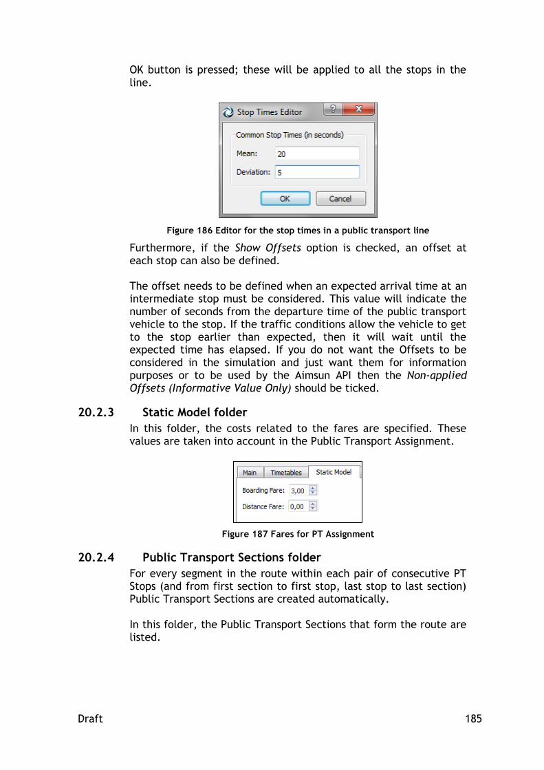
Draft 185
OK button is pressed; these will be applied to all the stops in the line.
Figure 186 Editor for the stop times in a public transport line
Furthermore, if the Show Offsets option is checked, an offset at each stop can also be defined. The offset needs to be defined when an expected arrival time at an intermediate stop must be considered. This value will indicate the number of seconds from the departure time of the public transport vehicle to the stop. If the traffic conditions allow the vehicle to get to the stop earlier than expected, then it will wait until the expected time has elapsed. If you do not want the Offsets to be considered in the simulation and just want them for information purposes or to be used by the Aimsun API then the Non-applied Offsets (Informative Value Only) should be ticked.
20.2.3 Static Model folder
In this folder, the costs related to the fares are specified. These values are taken into account in the Public Transport Assignment.
Figure 187 Fares for PT Assignment
20.2.4 Public Transport Sections folder
For every segment in the route within each pair of consecutive PT Stops (and from first section to first stop, last stop to last section) Public Transport Sections are created automatically. In this folder, the Public Transport Sections that form the route are listed.

Draft 186
Figure 188 List of Public Transport Sections that form the PT Route
20.2.5 Public Transport Assignment Outputs folder
One of the main outputs of a Public Transport Assignment is the PT Line loads, together with the boardings and alightnings. In this folder, this information is presented as a histogram and also in tables.
Figure 189 Line loads, boardings and alightnings for a PT Assignment
20.3 Public Transport Plan
A Public Transport Plan consists of a list of Timetables that will be used for each line included in it. As many PT Plans as required can be defined. All the existing PT plans are listed in the Project Window in the Public Transport Plans folder inside the Public Transport main folder. To create a new public transport plan select the New…/ Public Transport / Public Transport Plan option either in the Project Menu, in the Project Window Public Transport folder’s context menu or in the Project Window Public Transport Plans folder’s context menu. Once done, the new public transport plan will be listed in the Public Transport Plans folder in the Project Window.
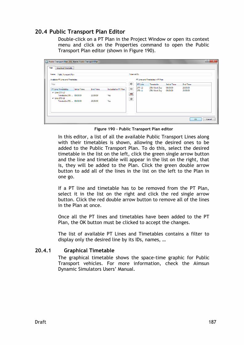
Draft 187
20.4 Public Transport Plan Editor
Double-click on a PT Plan in the Project Window or open its context menu and click on the Properties command to open the Public Transport Plan editor (shown in Figure 190).
Figure 190 - Public Transport Plan editor
In this editor, a list of all the available Public Transport Lines along with their timetables is shown, allowing the desired ones to be added to the Public Transport Plan. To do this, select the desired timetable in the list on the left, click the green single arrow button and the line and timetable will appear in the list on the right, that is, they will be added to the Plan. Click the green double arrow button to add all of the lines in the list on the left to the Plan in one go. If a PT line and timetable has to be removed from the PT Plan, select it in the list on the right and click the red single arrow button. Click the red double arrow button to remove all of the lines in the Plan at once. Once all the PT lines and timetables have been added to the PT Plan, the OK button must be clicked to accept the changes. The list of available PT Lines and Timetables contains a filter to display only the desired line by its IDs, names, …
20.4.1 Graphical Timetable
The graphical timetable shows the space-time graphic for Public Transport vehicles. For more information, check the Aimsun Dynamic Simulators Users’ Manual.

Draft 188
21 Subpaths
A subpath is a set of consecutive sections that can have any length and can be located anywhere on the model. Subpaths have two main uses:
To gather statistics for a stream.
To be used in rerouting traffic management actions as part of the new vehicle's route.
A network can contain as many subpaths as desired. All the existing subpaths are listed in the Project Window in the Subpaths folder inside the Infrastructure main folder. To create a new subpath, select the New…/ Infrastructure / Subpath option either in the Project Menu or in the Project Window Infrastructure folder’s context menu. Once done, the new will be added inside the Subpaths folder in the Project Window inside the Infrastructure main folder.
21.1 Subpath Editor
Double-click on a subpath in the Project Window or open its context menu and click on the Properties command to open the Subpath editor (shown in the figure below).
Figure 191 Subpath editor
The sections belonging to the subpath will be listed and highlighted in the active 2D view. The length of the sections plus turns that connect them will be displayed in the bottom part of the editor.

Draft 189
21.1.1 Editing a Subpath
To add sections to the subpath simply click on them in the 2D view. Sections are added after the currently highlighted section in the subpath list. If no section is selected the new section will be added as the last one. When the Autoconnect option is ticked, the editor automatically connects two unconnected sections using the shortest path (in distance) between the two (so it is not necessary to select each section individually, instead it is possible to select a section several sections ahead. If new sections must be added in the middle a route just select in the editor the preceding section and the start to click on the view for each new section. Pressing the [Ctrl] key while clicking on a section will add this section before the one selected in the list. If no section is selected the section will be added as the first one. The ‘Clear’ button will completely erase the route, while the ‘Delete’ button will just erase the selected section. It is possible to change the route order or a selected section using the Up and Down buttons. At any time and once the sections have been selected, the Check connectivity option will detect any unconnected pair of sections and warn accordingly.

Draft 190
22 Functions
The function editor allows the user to define cost functions using the Python language. Several types of functions can be defined:
Basic Cost Functions for the dynamic simulators
Cost Functions for the dynamic simulators using Vehicle Types
K-Initials Cost Functions for the dynamic simulators
K-Initials Cost Functions for the dynamic simulators using Vehicle Types
Route Choice Functions for the dynamic simulators
Macro VDF (Volume Delay Functions)
Macro TPF (Turn Penalty Functions)
Macro JDF (Junction Delay Functions)
Distribution + Modal Split
Public Transport Waiting Time
Public Transport Delay
Public Transport Transfer Penalty
Public Transport Boarding Function
Stochastic Utility Function
Adjustment Weight Function For an overview of the Python programming language and its syntax the reader is referred to the reference manual of python which can be found at: http://docs.python.org/reference/. In the following descriptions, all measurements have been expressed using the metric system. If the network has been built using English system units, the user should read miles instead of kilometres and feet instead of meters.
22.1 Basic Cost Functions / Cost functions using vehicle types
Basic Cost Functions allow the user to define, for each link, a generalised cost function not restricted to travel time only. These functions will be used in the Dynamic Route Assignment. They return the cost of a link without distinguishing per vehicle type. Therefore, they cannot make use of variables that have any vehicle type reference, so all vehicle types will have a common cost. The Cost functions using vehicle type are the same as the basic cost functions with the only difference that now the vehicle type can be used to distinguish between costs for vehicles.
Signature: cost(context, manager, section, turn, travelTime) double
where: context is a GKFunctionCostContext python object.
manager is a DTAManager python object. section is a DTASection python object.

Draft 191
turn is a DTATurn python object. travelTime is an unused object.
A complete overview of the methods that can be used for each object can be found in the Aimsun Scripting Documents. In this section the most common methods are mentioned and an example of a basic cost function will be given. The context object contains the user class for which the Volume Delay Function is being evaluated. In the case of a basic cost function this object will not be available. In the case of a cost function using vehicle type, the user class will provide the vehicle for which the function is being evaluated. The manager object contains the maximum section attractiveness, maximum turn attractiveness, attractiveness weight and user defined cost weight. The section object contains among others the section attractiveness, speed, length and capacity. The turn object contains among others the turn origin, destination, attractiveness, length and speed. The travelTime object which is not used. Example:
def cost(context, manager, section, turn, travelTime): time = section.getStaTravelT(manager) dist = section.length3D() w = manager.getUserDefinedCostWeight() aSec = section.getAttractiveness() aMax = manager.getMaxSectAttractiveness() attract = w * (1 - aSec/aMax) cost = time + dist + attract return cost
22.2 K-Initials Cost Functions / K-Initials Cost Functions using Vehicle Types
K-Initials Cost Functions allow the user to define, for each link, a generalised cost function not restricted to travel time only. These functions will be used in the Dynamic Route Assignment to calculate the K-Initial Shortest Paths. They return the cost of a link without distinguishing per vehicle type. Therefore, they cannot make use of variables that have any vehicle type reference, so all vehicle types will have a common cost. The K-Initials Cost Functions Using Vehicle Type are the same as the K-Initials Cost Functions with the only difference that now the vehicle type can be used to distinguish between costs for vehicles.
Signature: kinicost(context, manager, section, turn,
funcVolume) double

Draft 192
where: context is a GKFunctionCostContext python object.
manager is a DTAManager python object. section is a DTASection python object. turn is a DTATurn python object. funcVolume is the volume to evaluate this
function with. A complete overview of the methods that can be used for each object can be found in the Aimsun Scripting Documentation. In this section the most common methods are mentioned and an example of a basic cost function is given. The context object contains the user class for which the Volume Delay Function is being evaluated. In the case of a basic cost function this object will not be available. In the case of a cost function using vehicle type, the user class will provide the vehicle for which the function is being evaluated. The manager object contains the maximum section attractiveness, maximum turn attractiveness, attractiveness weight and user defined cost weight. The section object contains among others the section attractiveness, speed, length and capacity. The turn object contains among others the turn origin, destination, attractiveness, length and speed. The funcVolume object is the volume to evaluate this function with. Example:
def kinicost(context, manager, section, turn, funcVolume): dist = section.length3D()
cost = 10*funcVolume + dist return cost
22.3 Route Choice Functions
Route Choice functions are defined to be used as a user-defined Route Choice Model. They give the probability for a shortest path. Signature: rcf (context, manager, path, section, origin,
secondPath) double where: context is a GKFunctionCostContext python
object . manager is a DTAManager python object.
path is a DTAPossiblePath python object. section is a DTASection python object. origin is a DTACentroid python object. secondPath is a DTAPossiblePath python object.

Draft 193
The context object contains the user class for which the Route Choice Function is being evaluated. The manager object contains the maximum section attractiveness, maximum turn attractiveness, attractiveness weight and user defined cost weight. The path object contains variables for the path cost, travel time and distance. The section object contains among others the entrance section attractiveness, speed, length and capacity. The origin object contains variables for the entrances sections and percentages. The secondPath object contains variables for the path cost, travel time and distance for a second path to evaluate the function when needed. Example:
def rcf(context, manager, path, section, origin, secondPath): cost = path. getSPCurrentCost ( manager, context.userClass.getVehicle())
return cost
22.4 Macro Volume Delay Functions
The Macro VDF (Volume Delay Function) is used to model the travel time or the cost on a section or connection as a function of different parameters such as the volume of the section, its capacity, its length, etc. This type of function is taken into account when doing a static traffic assignment. For more information about VDFs and their role in the assignment, please refer to the Aimsun Macroscopic Modelling Manual. Section modelling:
Signature: VDF (context, section, volume) double where: context, section and volume are Python objects
of the following type: GKFunctionCostContext, CMacroSection and GKFunctionVolume.
A complete overview of the methods that can be used for each object can be found in the Aimsun Scripting Documents. In this section the most common methods are mentioned and an example of a basic Volume Delay Function is given. The context object contains the user class for which the Volume Delay Function is being evaluated. The section object contains the sections parameters that can be used in the macroscopic assignment. The parameters that can be consulted are: capacity, length, speed, user defined costs, additional costs, number of lanes and user defined attributes. The volume object contains the volume for which the Volume Delay Function must be evaluated. Three different volumes can be

Draft 194
consulted, total volume, volume per vehicle type and volume per user class. The Volumes are variable values that change during the assignment process. Function Body: In the body of the VDF any other arbitrary function that has been defined before the function declaration of the VDF can be used. Example:
def distance(context, section, volume): return section.length3D() / 1000.0 def tTime(context, section, volume): t0 = 60.0 * distance(context,section,volume) / section.getSpeed() c = section.getCapacity() v = volume.getVolume() t = t0 * ( 1 + 0.15 * (v/c)**4 ) return t def vToll(context, section, volume): t = 0.15 * distance(context,section,volume) return t def fToll(context, section, volume): t = section. getUserDefinedCost() return t def vdf(context, section, volume): c1 = 1.0
c2 = 0.1 purpose = context.userClass.getPurpose() if purpose != None: if purpose.getName() == “work”: c2 = 0.15 c3 = 0.2 time = tTime(context,section,volume) dist = distance(context,section,volume) toll = vToll(context,section,volume) toll = toll + fToll(context,section,volume) cost = c1 * time + c2 * dist + c3 * toll return cost
Connection modelling:
Signature: VDF (context, connection, volume) double where: context, connection and volume are Python
objects of the following type: GKFunctionCostContext, CMacroConnection and GKFunctionVolume.
A complete overview of the methods that can be used for each object can be found in the Aimsun Scripting Documents. In this section the most common methods are mentioned. The context and volume objects are the same as for the Volume Delay Function used for sections. The connection object contains

Draft 195
the parameters of the connection that can used during a macroscopic assignment. The parameters that can be consulted are: length and user defined attributes. Function Body: In the body of the VDF any other arbitrary function that has been defined before the function declaration of the VDF can be used. Example:
def vdf(context, connection, volume): length = connection.getLength() c1 = 0.05 return c1 * length
22.5 Macro Turn Penalty Functions
The Macro TPF (Turn Penalty Function) is used to model the travel time or the cost on a turn as a function of different parameters such as the volume of the turn, its length, etc. This function is taken into account when doing a static traffic assignment. For more information about TPFs and their role in the assignment, please refer to the Aimsun Macroscopic Modelling Manual.
Signature: TPF (context, turn, volume) double where: context, turn and volume are Python objects of
the following type: GKFunctionCostContext, CMAcroTurn and GKFunctionVolume.
A complete overview of the methods that can be used for each object can be found in the Aimsun Scripting Manual. In this section the most common methods are mentioned. The context and volume objects are the same as for the Volume Delay Function. The turn object contains the parameters of the turn that may be used during a macroscopic assignment. The parameters that can be consulted are: length, speed, additional volume, additional costs and user defined attributes. Function Body: In the body of the TPF any other arbitrary function that has been defined before the function declaration of the function can be used. Example:
def distance(context, turn, volume): return turn.length3D() / 1000.0 def tTime(context, turn, volume): t = 60.0 * distance(context,turn,volume) / turn.getSpeed() return t def tpf(context, turn, volume):

Draft 196
c1 = 1.0 c2 = 0.1 purpose = context.userClass.getPurpose() if purpose != None: if purpose.getName() == "work": c2 = 0.15 time = tTime(context,turn,volume) dist = distance(context,turn,volume) cost = c1 * time + c2 * dist return cost
22.6 Macro Junction Delay Functions
The JDF (Junction Delay Function) is used to model the travel time or the cost on a turn as a function of volumes of conflicting turns. This function is taken into account when doing a static traffic assignment. For more information about JDFs and their role in the assignment, please refer to the Aimsun Macroscopic Modelling Manual. Signature: JDF (context, turn, singleVolume, ownVolume,
conflictVolume) double
where: context, turn and singleVolume, ownVolume, conflictVolume are Python objects of the following type: GKFunctionCostContext, CMAcroTurn and GKFunctionVolume.
A complete overview of the methods that can be used for each object can be found in the Aimsun Scripting Manual. In this section the most common methods are mentioned. context and turn are identical to the context and turn of the TPF. singleVolume is the volume passing through the turn. ownVolume is the total volume of all the turns that share an origin lane with the turn. conflictVolume is the total volume of turns that geometrically conflict with the turn (automatic option) or the volume of turns specified by the user in the Conflict Turns table in the Node editor. Function Body: In the body of the JDF any other arbitrary function that has been defined before the function declaration of the function can be used. Example:
def jdf(context, turn, singleVolume, ownVolume, conflictVolume): volume = singleVolume.getVolume() conflict = conflictVolume.getVolume() ratio = 0.0 if ( volume != 0.0): ratio = conflict / volume

Draft 197
delay = 0.2 * ratio return delay
22.7 Macro Function Components
In the Functions folder we can also create Macro Function Components. They are used to get extra Outputs from the Static Traffic Assignment at the level of Sections, Connections and Turnings but also for Paths statistics. Any of the subfunctions in a VDF, TPF or JDF can be declared as a Component, by stating the key word which is the subfunctions name. Then, the code corresponding to this subfunction will be evaluated separately and a new column for sections, connections, turnings and paths will be created containing the subfunction values.
Figure 192 - Macro Function Component
The Function String must coincide with the name of the corresponding subfunction. Also, Derived Components can be declared, that is, the combination of other components. For example, if we create a Travel Time component and a Distance component, we can also calculate Speed without declaring it as a subfunction in the VDF, TPF or JDF, but as a combination of the existing components, as shown in the image below. Defining the Speed as a derived component will give us the path mean speed, whereas defining it as a non-derived component would add up the speeds through the path.

Draft 198
Figure 193 Macro Function Derived Component
22.8 Stochastic Utility Functions
The SUF (Stochastic Utility Function) is a utility function that is used to calculate the probabilities each path is being used. This function is taken into account when doing a Stochastic Traffic Assignment. For more information about SUFs and their role in the assignment, please refer to the Aimsun Macroscopic Modelling Manual.
Signature: SUF (context, pathChoice) double
where: context and pathChoice are Python objects of the following type: GKFunctionCostContext and GKPathChoice.
A complete overview of the methods that can be used for each object can be found in the Aimsun Scripting Manual. In this section the most common methods are mentioned. context is identical to the context of the VDF. pathChoice is a set of paths and their costs. Example:
def suf(context, pathChoice): mu = 100 total = 0.0 cost = 0.0 res = [] for pathCost in pathChoice.getCosts(): total += math.exp( mu * 1.0/pathCost ) for pathCost in pathChoice.getCosts(): res.append( math.exp(mu* 1.0/pathCost) / total ) return res
22.9 Distribution + Modal Split Functions
The DMS (Distribution + Modal Split Function) is used to model the resistance to make a trip with each of the available Transportation

Draft 199
Modes. This function is taken into account when executing the Distribution + Modal Split process. For more information about DMSs and their role in the Four-step Model, please refer to the Aimsun Travel Demand Modelling Manual.
Signature: DMS (mode, cost) double
where: mode is a Python object of type GKTransportationMode and cost is a double.
A complete overview of the methods that can be used for each object can be found in the Aimsun Scripting Manual. In this section the most common methods are mentioned. mode is a Transportation Mode and cost is the skim matrix value. Example:
def dms(mode, cost): res = 0.0 name = str(mode.getName()) if name == “Car”: res = 100.0 * math.exp(-0.00008*cost**3) if name == “Bicycle”: res = 70.0 * math.exp(-0.0005*cost**3) return res
22.10 Public Transport Waiting Time Functions
The PWF (Public Transport Waiting Time Function) is used to model the waiting time on a Public Transport Stop until boarding a vehicle. This function is taken into account when doing a Public Transport Assignment. For more information about PWFs and their role in the Public Transport Assignment, please refer to the Aimsun Travel Demand Modelling Manual.
Signature: PWF (context, interval) double
where: context is a Python object of type GKFunctionCostContext and interval is a double.
A complete overview of the methods that can be used for each object can be found in the Aimsun Scripting Manual. In this section the most common methods are mentioned. context gives the experiment context and interval is the combined mean headway between public transport vehicle arrivals of the possible boarding lines. Example:
def pwf( context, interval ): frequency = 60.0 / interval res = 20.0 * math.exp(-0.3 * frequency)

Draft 200
return res
22.11 Public Transport Delay Functions
The PDF (Public Transport Delay Function) is used to model the travel time or the cost on a Public Transport Section (that is, the in-vehicle time). This function is taken into account when doing a Public Transport Assignment. For more information about PDFs and their role in the assignment, please refer to the Aimsun Travel Demand Modelling Manual.
Signature: PDF (context, line, ptsection) double
where: context, line and ptsection are Python objects of the following type: GKFunctionCostContext, GKPublicLine and GKPTSection.
A complete overview of the methods that can be used for each object can be found in the Aimsun Scripting Manual. In this section the most common methods are mentioned. context is identical to the context of the PWF. line is the volume Public Transport Line. ptsection is the Public Transport Section being evaluated. Example:
def getFare( line, ptsection ): distFact = line.getDistanceFare() distance = ptsection.getDistance() res = distFact * distance return res def pdf( context, line, ptsection ): inVehicleTime = 0.0 distance = ptsection.getDistance() speed = 25.0 inVehicleTime = distance / speed fare = getFare(line, ptsection) c1 = 1.0 c2 = 1.0 res = c1 * inVehicleTime + c2 * fare return res
22.12 Public Transport Transfer Penalty Functions
The PTP (Public Transport Transfer Penalty Function) is used to model the penalty for doing a transfer from line to line during a public transport trip. Usually people avoid transfers in public transport because of the discomfort they produce, so this function will penalise the decision to make a transfer. For more information about PTPs and their role in the Public Transport Assignment, please refer to the Aimsun Travel Demand Modelling Manual.

Draft 201
Signature: PTP (context) double
where: context is a Python object of type GKFunctionCostContext.
A complete overview of the methods that can be used for each object can be found in the Aimsun Scripting Manual. In this section the most common methods are mentioned. context is identical to the context of the PWF. Example:
def ptp( context ): res = 7.0 return res
22.13 Public Transport Boarding Functions
The PBF (Public Transport Boarding Function) is used to model the cost for boarding a public transport vehicle. This function is taken into account when doing a Public Transport Assignment. For more information about PBFs and their role in the assignment, please refer to the Aimsun Travel Demand Modelling Manual.
Signature: PBF (context, line, stop) double
where: context, line, and stop are Python objects of the following type: GKFunctionCostContext, GKPublicLine and GKBusStop.
A complete overview of the methods that can be used for each object can be found in the Aimsun Scripting Manual. In this section the most common methods are mentioned. context is identical to the context of the PWF. line is the Public Transport Line the passenger wants to board to. stop is the stop at which the passenger is waiting to board. Example:
def pbf(context, line, stop): res = line.getBoardingFare() return res
22.14 Adjustment Weight Functions
The ADW (Adjustment Weight Function) is used to give different (not fixed) weights to the counts (to the difference between counts and assigned volumes) in the adjustment process. It returns a value that multiplies the Reliabilites previously set by the user (1 by

Draft 202
default). This function is taken into account when doing an Adjustment. For more information about ADWs and their role in the Adjustment, please refer to the Aimsun Macroscopic Modelling Manual.
Signature: ADW (observed) double
where: observed is a double. observed is the value in the Time Series used in the Adjustment, the count that has to be compared with the assigned volume. Example:
def adw(observed): res = 1.0
if observed>0.0: res = 1.0/math.pow(observed,0.5) else: res = 0.0 return res
22.15 Function Editor
Using the editor, the function can be renamed; its type can be selected among the available ones (cost, cost with vehicle type, route choice, macro volume delay function, macro turn penalty or junction delay function) and its definition (or function code) can be written. In the current version, this definition is set by typing it in the function code box. To ease the task a button that verifies if the code is right (in terms of following the predefined function items) or wrong is also available. When pressing the Verify button a window informs the user if the function is well written or it indicates where the first error is found.

Draft 203
Figure 194 Function Editor
A graph can also be drawn by selecting a specific experiment, a specific vehicle type and the trip purpose (if applicable). The Usage folder shows how many objects use this function, colouring them in the active 2D view.

Draft 204
23 Grouping Categories
A Grouping Category is an Aimsun object type and can keep as many groupings as desired. Having groupings allows to automatically obtain the mean or average data of the objects included in the grouping. It is easy to get the number of vehicles generated in a certain area or the mean speed of all the sections entering a particular neighbourhood, for example. Screen lines can also be calculated by means of groups. To create a new Grouping Category object right click on the DATA ANALYSIS folder in the Project window and select New/Grouping Category.
Figure 195 - New Grouping Category Object context menu
Open the Grouping Category editor to define the type of objects it will contain. If the Groupings inside the Grouping Category cannot share objects, then the Exclusive Objects checkbox must be checked.
Figure 196 - Grouping Category editor
23.1 Grouping
A Grouping is a set of objects of the same type (defined inside a Grouping Category). It can also be linked to an area defined by a polygon. There are two ways of creating a Grouping: The first option is available from any Grouping Category object New.../Grouping context menu. The second option becomes available after building a Polygon object. Right click on it and select Convert To/ Grouping.

Draft 205
After converting a Polygon into a Grouping, the following dialog pops up to select the Grouping Category that you want to add the new Grouping to.
Figure 197 - Grouping Category Selection
Double click on any Grouping object to access the list of objects belonging to the Grouping and edit it. In addition to adding an object to the grouping, the user can set an And or Or. Usually all the objects will be added with an And, but for some usages of the Groupings the Or may be useful, for example for a Link Analysis of paths that either use a section X or a section Y. And takes precedence over Or.
Figure 198 Group Editor
23.1.1 Grouping Object Selection
It is possible to add objects to a Grouping in four different ways:

Draft 206
Once the Grouping editor is open, by clicking on objects that
have the same type than the type defined in the Grouping
Category.
Having selected some objects in the 2D View and clicking
Add Selection button in the Grouping editor.
For those Grouping Objects that are linked to a polygon area,
select Build option in the Grouping Category context menu.
It will automatically calculate which objects are inside the
Grouping areas and add those that belong to the Grouping
Category Object Type.
Figure 199 Grouping Category Build
For those Groupings linked to a polygon area, select Build
option in the Grouping context menu. It will automatically
calculate which objects are inside the Grouping area and add
those that belong to the Grouping Category Object Type.
Figure 200 Grouping Build
23.1.2 Grouping Statistics
After simulating a network, the Refresh Statistics option, available in the Grouping Category context menu, calculates for all groupings the aggregation or mean (depending on the Time Series aggregation type) of all available statistics in the Grouping objects. It is also available at a Grouping level to calculate just the statistic for the specific grouping.
Figure 201 Refresh Statistics for all the Groupings of a Grouping Category

Draft 207
24 Network Attribute Overrides
One of the reasons to create different Aimsun .ang files for each scenario you want to simulate or assign is to change attribute values that are used in the simulation or assignment process but cannot be modified with traffic management actions, such as section distance zones, capacities, section VDFs, turn penalties and so on. The aim of the Network Attribute Override objects is to allow the modification of those attributes without having to replicate networks for each configuration. To create a new Network Attribute Override object, select Project/New/Network Attributes Override menu Double click on it and the following editor will bring up:
Figure 202 - Network Attributes Override Editor
To add new objects, the user has to click over, select the object and the attribute to override, then press the Add (+) button Once the object has been added, it is possible to change the attribute as desired.
24.1 Applying the Overrides
From any experiment main tab folder (see Figure 203), it is possible to select which overrides you want to apply before starting the simulation or assignment process.

Draft 208
Figure 203 Override object selection
Note that the original values in the Aimsun network are always kept and the changes defined in the overrides are only present in the static or dynamic simulation model.

Draft 209
25 Connection Tool
The connection tool is used to create connections between two objects. These connections can be between centroids and sections, centroids and nodes, controllers and detectors ... But also, they can be used between two sections to create a turn.
25.1 Connection tool to create connections
To create all types of connections between objects, click on the Connection tool. The use of the Connection tool to create turns between sections is more complex than the other cases so it is explained in detail in the next section. Click once if only one connection must be created or double click to activate it in continuous mode if more than one connection must be created.
Figure 204 Connection Tool
After that, click on the object that will be the origin of the connection and without releasing the mouse button drag the mouse to the destination object of the connection. Finally, release the mouse on the destination object and a new connection will be created. In the case of centroids, when the Connection tool is selected if the user clicks on the centroid and without releasing the mouse button moves the mouse to the desired section or node and then releases the mouse, a ‘To’ connection will be created. If the mouse click starts on a section or node and ends on the centroid then a ‘From’ connection will be created.
25.2 Connection tool to create turns
To use the connection tool to create turns, first click on the tool, then press on the origin section of the turn and without releasing the mouse move it to the destination section. When the mouse button is released, the connection, that is a node with a single turn, is added.
Figure 205 Creating a node using the Connection Tool
If the user wants to add more than one turn to the same node using the connection tool and the sections involved in the second turn do

Draft 210
not belong to the node yet, just select the node before creating the second turn. Remember that the tool can be used in continuous mode (by double-clicking on it) if more than one turn is to be added. The behaviour of the connection tool when connecting two sections is the following one:
If the Ctrl key is pressed while creating the connection, a turn from all the origin lanes to all the destination lanes will be created.
If the Ctrl key is not pressed while creating the connection, when the number of origin and destination lanes is different, for the turn the section with fewer lanes will be matched with the closest lanes in the other section. See Figure 206 for details.
Figure 206 Creating a turn with the connection tool
If the Ctrl key is not pressed and the origin section or the destination one have all its lanes already involved in a turn, then the new turn will use the rightmost or leftmost lane of the sections that have all their lanes already involved in turns or the lanes that are still not assigned in the sections if any. In Figure 207, an example where the origin section has all its lanes already involved in a turn is shown.
Figure 207 Creating a turn with the connection tool
The connection tool tries to ease the process of creating the geometry but at anytime the node editor can be opened to refine the turns created or to create special turns that cannot be created using this tool.

Draft 211
26 Find
Aimsun includes a find box that allows objects to be found by any of their attributes. For example:
Find all sections whose speed is lower than 50 km/h.
Find all centroids connected to one object.
Find all VMSs in the network displaying a message (during a simulation).
Figure 208 Find all the centroids connected to one object
The find dialog allows the user to specify an alphanumeric value, an attribute, a particular type of object and an operator. The attribute list varies in function of the object type (i.e. number of lanes for a section, messages for a VMS…). The user can select the operators:
=: the value of the attribute of the objects the user is looking for must be equal to the given value.
<>: the value of the attribute must be different.
>: the value of the attribute must be greater than the given value.
<: the value of the attribute must be lower than the given value.
[]: range, a second field appears. The value of the attribute must be in the range.
~: the found value matches the given regular expression (Perl's regexp language).
It is possible to set All as the attribute to be used. In this case, the dialog will look for the value in the Find field in all the attributes of each object.

Draft 212
It is also possible not to set a specific value in the Find field, using the character ‘*’. A search of this symbol will produce a list of all the objects specified in the Type field, whatever their attributes are. The result of a search will appear in the find dialog as a result list. It will show the object type (section, node, centroids, O/D matrix,…), the ID, name and the value of the used attributed. If the All attribute is used, the found value and the attribute in which the value was found will be shown. It the result of the search include graphical objects, they can be selected by using the Select Results in view option.
26.1 Working with Search Results
Graphical objects, when selected in the result list, will be highlighted using the primary mark colour. A double click on any item in the list will open the editor for this object.
26.1.1 Refining a Search
The Find in Results button activates a second search, based on a different criterion, but this time only among the objects found on the first search (to refine the search).
26.1.2 Result Selection
The Select Results selects on the view all the found graphical objects (non-graphical objects will not be selected).
26.1.3 Use of the Context Menu
Select any item in the result list and press the right button to bring its context menu. In a graphical view, commands in the context menu are applied when possible to all the selected graphical objects and not only to the object that brought out the context menu. On the other hand, commands executed from the search result list are executed only on the object that brought the context menu. It is possible, however, to execute a command for more than one object in the search result list. Use the Select Results button and then execute the command from the view.

Draft 213
27 Table View
Aimsun provides a new way of accessing and modifying data of Aimsun objects. It can be opened via the Window->Windows menu or using the W quick shortcut.
Figure 209 An empty table view
On a regular Table View, there are six main interaction areas:
Type: Lets the user choose which Type should be listed on the Data View.
Show: Lets the user choose which objects of the current type should be shown on the Data View.
o All: Shows all the objects of the current type. o Selected (in View): Shows the objects of the current
type that are selected in the current view. o Filter: Lets the user define a condition to filter which
objects of the current type should be shown. o Filter Selected (in View): Lets the user define a
condition to filter which of the objects of the current type that are selected in the current view should be shown.
Configuration: Lets the user choose which Table View configuration to use.
Action: The Action button lets the user do some miscellaneous actions:
o Column Visibility: Specifies which columns to show o Show Inherited Types: Specifies whether to show or
not objects of types that inherit from current type, for example, having it checked would show also SubNetworks when Type is Polygon
o Save Configuration: Lets the user save the current Table View Configuration
o Delete Configuration: Lets the user delete saved Table View Configurations
o Copy: Copies data from the either the Data or the Summary View
The Data View: Shows the data of all the objects that should be shown according to the specified options

Draft 214
The Summary View: Shows the common data of all the objects that are shown on the Data View
27.1 The Data View
The Data View is the main part of the Table View. It is a table where each column represents a property of the given type and each row represents an object of the given type.
Figure 210 Table View showing polygon data
Columns of the Data View might be editable or not. For example, the number of connections of Centroids is not editable while the brush style of a Polygon is. To edit a given value, just double click in the appropriate cell and an editor suitable for the column data type will appear. Remember to press Return to finish data modification. When an object is selected in the Data View, it will appear marked in the View if it is a View object. Double clicking on the ID will centre the object in the View if it is a View Object.
27.2 The Summary View
The Summary View shows the same columns than the Data View but only one row. In that row, each cell will be empty if not all objects of the Data View have the same value in that column or will have the value of all objects of the Data View if they are the same. Changing the value of a column in the Summary View changes the value of that property for all objects shown on the Data View.
27.3 Filtering
The Table View provides filtering options to restrict the objects shown on the Data View. Filtering works over any or a particular Attribute of the current Type and the user can choose six different filtering methods over that attribute.
=: the value of the attribute of the objects the user is looking for must be equal to the given value.
<>: the value of the attribute must be different.

Draft 215
>: the value of the attribute must be greater than the given value.
<: the value of the attribute must be lower than the given value.
~: the found value is matched by the given regular expression.
[]: range, a second field appears. The value of the attribute must be in the range.
27.4 Column Visibility
Types often have many attributes and sometimes it is interesting to show only some of them. Using the column Visibility dialog it is possible to choose which columns should be shown and which ones should be hidden.
Figure 211 Editing the visibility of some columns
27.5 Configurations
Configurations are predefined queries for the Table View. A configuration stores:
The type
The visible columns
The show mode
Filtering options
The current configuration can be changed using the Configurations option list. Configurations can be saved and deleted using the Action Menu.

Draft 216
28 Inspector Window
The Inspector Window allows you to quickly check and modify attributes of the selected objects, or to look at their time series, if any. Go to Window / Windows / Inspector or use the I quick shortcut and a window will pop up showing the attributes of the currently selected objects as seen in the images below.
Figure 212 Opening the Inspector Window
Figure 213 Inspector dialog
28.1 Main View
The Inspector will display suitable editors to see and edit attributes of the selected objects. Just change the value of the corresponding field, and the attribute is directly modified, without the need of any validation – but remember that you can always cancel the modification with the Undo command. Similarly to the Table View, some of the attributes might not be editable.

Draft 217
28.2 Multiple Selection Editing
If the selection contains various objects, you will be able to edit all of them at the same time, similarly to the Summary of the Table View. Likewise, for a given attribute, the field appears blank if the selected objects have different values. If the selection contains objects of different types (p.e. three Sections and two Turns), only the attributes they have in common will be displayed.
28.3 Time Series
Along with the ‘Main’ tab where you can edit the objects’ attributes, the Inspector offers a ‘Time Series’ tab. In this tab, you can visualize the Time Series exactly as you would do in a typical object editor, at the difference that you can only see the Time Series of one variable at a time. In counterpart, as you can select various objects at a time, the ‘Time Series’ tab will display the variables of all of them in the same graph.

Draft 218
29 Dynamic Labels
Dynamic label functionality provides a method of displaying both static and dynamic information about network elements as textual labels. To add a dynamic label to an element, right click on the element in the 2D view to access its context menu, then select Dynamic Labels / Attribute Dynamic Label.
Figure 214 Dynamic Labels Context Menu
Select the required label, in this case, the detector name,
Figure 215 Dynamic Label Attribute Editor
Check tick boxes to show attribute name, units, change the colour or the font size if required, then select OK in the editor. The label will appear over the element, but it can be dragged to any desired position.

Draft 219
Figure 216 Label positioning
Multiple labels can be added, in this case the SI Section Speed as well as the name.
Being dynamic, labels are updated with relevant information, for example during a running simulation.

Draft 220
Labels may be added to more than one element at once by selecting all (for example by holding down the [Shift] key) then selecting from the context menu on a selected element as normal.
Dynamic labels may be closed by selecting the label or labels, and either pressing the [Delete] key, or by selecting Dynamic Labels / Close / Selected from a label’s context menu. Selecting Dynamic labels / Close / All closes all labels in the view, while Dynamic Labels / Close / Equal closes all labels in the model of the same type as the first label selected.
There is another kind of Dynamic Labels, which are specific to show Turn Attributes. See the Aimsun Dynamic Simulators Users’ Manual for a detailed explanation.

Draft 221
30 Printing
Aimsun offers tools for printing the active 2D view either in a printer or to a PDF document for any paper size and orientation.
30.1 Direct Print
Use the Print command from the File menu to print the current 2D view. A dialog will appear asking for the printer and the printer’s settings. From this dialog, the user can select to print the entire network or just the visible area in the current view. To do so select, in Page Range, select All to print the whole network or Selection to print the current view area.
30.1.1 Print Preview
The Print Preview command, from the File menu, will open a dialog allowing the user to prepare the document for printing and reviewing the final result.
Figure 217 Print Preview dialog
Both the Print and the Export PDF will use the settings set using the Page Setup command. This command allows the user to select the

Draft 222
paper size, orientation, printer, colour print… Finally, one can also select the Drawing Mode to be printed.
30.1.2 Export to PDF
This command creates a new PDF document printing either the whole network or the visible area as seem in a 2D view. It will ask first for the name of the PDF file to be created and then for the printing preferences as paper size and orientation.
Figure 218 Export to PDF settings
30.2 Print Layout [Fast track: July 2013]
The Print Layout allows you to compose a graphic scene on a page,
including elements such as views of the network, legends, text, Time
Series graphs, or images. You can then print the Print Layout, or export it
to a PDF or an image.
30.2.1 Creation
To create a new Print Layout, right-click on the Data Analysis folder in the Project Dock, and choose New/Print Layout; to edit it, double-click on it in the Project Dock.
30.2.2 Wizard
When editing a new layout (or any empty layout), before displaying the actual layout editor, you will be presented the Print Layout Wizard dialog. This dialog will help you to quickly and easily fill a Print Layout with a title, a subtitle, 1 or more maps or images, and other common elements.

Draft 223
30.2.2.1 Page Settings section
In the Page Settings section, you can define the page format to use for the Print Layout: either a standard one, or a custom format. Note about custom formats: when using a custom format, the Print Layout will actually use a standard format, and adjust the margins to match the custom parameters. It's most likely that your printer won't allow you to print a custom format page, but there are no such constraints with images: you can use custom formats to export the Print Layout to an image of any dimension.
30.2.2.2 Layout Composition section
Here you can define which elements to include in your Print Layout:
A title, a subtitle, a text containing document information (note
that by default, some special variables are used in this text.
Special variables for text are detailed below.), and a footer text.
The central part of the Print Layout will be occupied by one or
several maps, Time Series graph, or images. They can be laid out
vertically, horizontally, or in a grid.
by default, by creating a map element, a scale, a legend,
and a label indicating the view's time context will also be
created ;
by default, by creating a Time Series graph element, a
label indicating the graph title (automatically updated
according the displayed Time Series) will also be created ;
optionally, an individual footer label that will be created
and placed at the bottom of each element.
Clicking on Ok will create and fill the Print Layout with the chosen elements; then you will only have to configure the specific parameters of each element (map region and view mode, image file, etc.) to obtain the desired Print Layout.

Draft 224
You can also click on Ignore to leave the Print Layout empty.
Figure 219 The Print Layout Wizard: setting up a Landscape A4 Print Layout with the central spaced shared horizontally by 2 elements: a map and an image.
30.2.3 Editor
The Print Layout editor will allow you to configure the specific parameters of each element, add new elements or remove existing ones, change the page format, and more importantly, print or export the Print Layout to PDF or an image file. At the center of the Print Layout editor, you can see a preview of the Print Layout. Use the zoom in/out buttons in the top tool bar, or your standard keyboard shortcuts for zooming in/out (Ctrl+Plus and Ctrl+Minus on Windows), to zoom in/out the preview.

Draft 225
Figure 220 The Print Layout Editor showing the resulting Print Layout of the wizard example, configured with a view mode and an image. The title element is currently selected, for example to edit its text.
30.2.3.1 Configuring the elements
To configure an element, select it by clicking on it (you can select several elements at a time with Ctrl+click, or by selecting): you will see its attributes displayed in the editor at the right side of the preview.
General attributes. All the elements have those attributes in
common:
X,Y, Width and Height: they are expressed in % of the page
and allows to define the position and size of an element.
You can move the selected elements by drag & drop, and
resize them by moving their edges. You can also move the
selected elements by 1% increments using the keyboard
arrows.
Background: check it to draw an opaque background for the
element, and define its colour with the Colour button.
Draw frame: check it to draw a black frame at the border
of the element.
Z-ordering: click on 'To front' or 'To back' to bring the
element to the foreground or send it to the background.
Map:
When a map element is selected, you can check "Enable
Pan & Zoom Edition" to change the visible region of a map
by drag & dropping (exactly like the Pan of Aimsun's main
view) or using your mouse wheel. You can also set the
visible region using the editor's Center and Scale fields.
Time: to define the time context of the view.
Mode: to define the View Mode to be used on the view.

Draft 226
Legend
Scale: changes the size of the font and of the legend's
items.
Mode: defines the mode to be shown by the legend. If the
legend element is above a map element, you can leave it
to 'Automatic' and the legend will use the mode defined in
the map element.
Style: defines the style to be shown by the legend, or
shows all the mode's styles if set to 'All'. Note that by
default, the selected style is the first color style of the
mode, as it is the most likely to be the interesting one.
Scale
The scale element will display the scale used by the map
element below it. If the scale is not above a map element,
it will show the scale of the closest map element.
Show Scale Label: check it to show the scale value in
"1:xxxx" format.
Time Series graph
This element displays Time Series graphs in the same way
as the Time Series Viewer.
To add Time Series to the graph, select it: a widget similar
to the Time Series Viewer appears and allow you to add
Time Series to your graph and configure it.
To have more details on how to use the Time Series
Viewer, see: 35.2 Time Series for Multiple Objects.
Text
The text of the text element supports special variables,
that are automatically replaced by the corresponding
value:
- ${A_AUTHOR}: author of the document
- ${A_VERSION}: Aimsun version
- ${A_PATH}: document path (file name not included)
- ${A_FILE_NAME}: document file name
- ${A_VIEW_CONTEXT}: underneath view's context
- ${A_VIEW_CONTEXT_NO_DATE}: underneath view's
context without date
- ${A_DATE}: current date
- ${A_TIME}: current time
- ${A_DATE_ISO}: current date in ISO format
- ${A_TIME_ISO}: current time in ISO format
- ${A_TIMESERIES_GRAPH_TITLE}: underneath Time Series
graph's title
You can also change the font, font size, color and
alignment of the text.
Image
By clicking on the 'Browse' button, you can choose in your
file system the image to be shown.

Draft 227
Line
The line element draws vertical, horizontal and diagonal
lines. The color of the line is always black.
30.2.3.2 Adding and removing elements
To create a new element, click on one of the buttons in the left tool bar. The corresponding new element will be added around the center of the Print Layout. You can also create new elements using the Copy-Paste keyboard standard shortcuts: select some elements and trigger the copy shortcut (Ctrl+C on Windows); then trigger the paste shortcut (Ctrl+V on Windows) to create clones of the items. To remove one (or several) elements, select it and press the delete key.
30.2.3.3 Configure the page format
To change the page format, click on the 'Page Format' button in the top tool bar. If you want to use a custom format (to export an image of specific dimensions), choose one of the standard page format, and adjust the margins to match your needs.
30.2.3.4 Exporting the Print Layout
There are 3 ways to export the print layout. Print
Export to PDF
Export to Image: creates a PNG image. The pixel size of the image
will be 4 times bigger than the defined size of the layout in points
(ex: 500 points width -> 2000 pixel width). Margins of the page are
not included in the image.
Note that only 'Export to Image' supports custom page formats.

Draft 228
31 Colour Ramps
A colour ramp is a predefined group of colours used in Aimsun to colour a group of objects when drawing in a 2D view depending on any objects attribute. They are also used to colour the selected object. In Aimsun, several colour ramps are used. These colour ramps are:
MARK_COLORS: defined in the mark.xml file and used, for example, to colour the selected objects
TIME_SERIES_WIDGET: defined in the lines.xml file and used when drawing the time series graphics.
ASSIGNED_VOLUMES: defined in the assignedVolumes.xml file and used in the Aimsun Macro component when showing the static assignment results. See the Aimsun Macroscopic Modelling manual for more details.
The colour ramps are defined in xml files that are located in the <AIMSUN_HOME>/shared/color_ramps folder. There is an xml file for each colour ramp. The way to change the colours in a colour ramp is to edit directly the xml file. The format of the colour ramps xml files is: <color_ramp name="RAMP_NAME" type="RAMP_TYPE" coded="RAMP_CO/DED"> <color>COLOR_DATA</color> <color>COLOR_DATA</color> ... </color_ramp>
where:
RAMP_NAME: it is the name of the ramp.
RAMP_TYPE: it is the colour space to be used when interpolating, either RGB or HSV.
RAMP_CO/DED: how colours are specified, either HEX or DECIMAL
COLOR_DATA: the colour information. The format varies according to RAMP_CO/DED:
o HEX: #RRGGBB, where: RR is the hexadecimal red component from 00
to ff GG is the hexadecimal green component from
00 to ff BB is the hexadecimal blue component from 00
to ff o DECIMAL: RRR GGG BBB (space separated), where:
RRR is the decimal red component from 0 to 255
GGG is the decimal green component from 0 to 255

Draft 229
BBB is the decimal blue component from 0 to 255
Note that colours are specified in RGB. The RAMP_TYPE is used only in the interpolation. Example 1: a gray ramp using HEX <color_ramp name="GRAY" type="RGB" coded="HEX"> <color>#000000</color> <color>#ffffff</color> </color_ramp>
Example 2: a gray ramp using DECIMAL <color_ramp name="GRAY" type="RGB" coded="DECIMAL"> <color>0 0 0</color> <color>255 255 255</color> </color_ramp>

Draft 230
32 Modes and Styles in 2D Views
Aimsun can show any graphical object in several ways based on the values of its attributes. It can also show these attributes as labels on the network. For example, it can show sections with a speed of 50 Km/h in red, 60 Km/h in blue… or it can draw bars of 3 meters width on sections with a density of 1000 and bars of 6 meters width on the ones with a density of 2000.
32.1 View Styles
These effects are achieved using View Styles. To create a new View Style select the New…/ Data analysis / View Style option in the Project Menu, or in the Project Window Data Analysis folder’s context menu or in the Project Window View Styles folder’s context menu. Once done, the new View Style will appear in the View Styles folder inside the Data Analysis main folder in the Project Window. Open the Style editor by double-clicking on it. A View Style contains information on:
The type of object to be drawn (sections, nodes, centroids, polygons…)
The value of a selected attribute it will be based on (speed, capacity, mean queue, length…). The value can be that of an attribute or the value of an attribute divided by other attribute. Also the values can be normalised if the Normalise tick is checked resulting in values ranging from 0.0 to 1.0.
The style chosen to draw the object (in red colour, using a width of 3 meters, …)
The conditions on when to apply this style, either for a predefined zoom range or based on the value of an attribute.
The following table shows the different ways the object may be drawn:
Type Effect
Colour Changes the colour
Pen Width Changes the pen width
Pen Style Changes the pen style
Brush Style Changes the brush style
Spot Draws extra information over the object
Hide Hides the object (it will not be drawn)
Colour Opacity Changes the opacity of the colours defined in another style
Attribute Adds a label with the value of the specified attribute
Diagram Draws a diagram (circles, pies, histograms...) on each object

Draft 231
After selecting the object, the attribute, and how it will be drawn, different values for the effect must be selected (for example different colours) based on the values of the selected attribute. An attribute can be either continuous or discrete. The user will group continuous values using ranges. Discrete values cannot be grouped. For each discrete value or each range of continuous values, the final effect can be modified (see Figure 221). The user can use the Calculate Ranges button to calculate automatic ranges. When a label is displayed, the number of decimal digits to use in the label can also be specified. When defining a style that displays a label or a spot, the units of the specified size can be defined, that is, if the value specified is in meters or pixels.
Figure 221 View Style Editor – Main folder
In the Conditions folder (see Figure 222), the zoom range this style will be visible can be specified as well as if the style is going to be applied to a subset of objects. This subset can be specified by

Draft 232
selecting the attribute to filter objects by and the range of matching values to apply the view style.
Figure 222 View Style Editor – Conditions folder
32.2 View Modes
Several styles can be combined into one View Mode. The user will then select, among all the available modes, which one will be applied to the current view. To create a new View Mode select the New…/ Data Analysis / View Mode option either in the Project Menu, in the Project Window Data Analysis folder’s context menu or in the Project Window View Modes folder’s context menu. Once done, the new View Mode will appear in the Project Window inside the Data Analysis main folder. Open the Mode editor by double-clicking on it.
Figure 223 View Mode Editor

Draft 233
In the View Mode editor, the user can assign styles to the mode. The dialog offers two lists with styles. The list above contains all the styles that are not in the current mode. The list below contains the styles that are already assigned to it. Use the arrows to add or remove styles to/from the mode. When drawing styles using spots, the user can select when these spots are drawn: either after drawing all the objects in the layer (in this case the spots will be over the objects) or before drawing the objects (in this case the sport will be behind the objects). If the style uses big spots is a good idea to draw them behind the objects to clarify the plot. A second option can be used to set the drawing orders of objects in a layer (each layer will be draw in the order specify by its level) based on the value of the attribute used in one of the styles in the mode. The sorting will occur only when selecting the view mode. Combined with the previous option can help to clarify a view mode (for example when drawing isochrones). It is also possible to set the view mode automatic activation:
Never: it will never be activated automatically.
Micro: it will be activated when a Microscopic simulation
finishes.
Meso: it will be activated when a Mesoscopic simulation
finishes.
Macro: it will be activated when a Macroscopic Traffic
assignment finishes.
Hybrid: it will be activated when a Hybrid simulation
finishes.
Dynamic: it will be activated when a dynamic simulation is
running.
Paths: it will be activated when checking the paths from any
dialog (i.e. Replication editor: Path Assignment tab folder).
32.3 Examples
The following example will create a View Mode that colours the vehicles according to their origin centroids.

Draft 234
Figure 224 - Vehicle by Origin Style
Create a New Mode and call it Vehicles by Origin. Create a new Style and add it to the new mode. Edit the new style. In the style editor, shown in Figure 224, choose Simulation Vehicle as the Type, and Origin as the Attribute. Change the type of the variable to Discrete. Keep Colour as the Representation. Press the Calculate Ranges button. In the Automatic Ranges Calculator dialog (Figure 225), choose Unique Values as the Method. Press Calculate to get all the unique values. Press OK.

Draft 235
Figure 225 Unique Values Classification
Edit the ranges if necessary. Select the new mode from the Drawing Mode list in the current view.

Draft 236
Figure 226 Vehicles by Origin Mode in action
Next example will create a View Mode where centroids are hidden. Create a New Mode and call it Hide Centroids. Create a new Style and add it to the new mode. Edit the new style. In the style editor, shown in Figure 227, choose Type: Centroid, and Attribute: ID. Set the type of the variable to Continuous, and the Representation to Hide. Press the New button and set the range to 0.00 – inf.

Draft 237
Figure 227 Hide Centroids View Style
Figure 228 shows the network with the Drawing Mode set to Hide Centroids.
Figure 228 Drawing Mode ‘Hide Centroids’

Draft 238
32.4 Wizards
There are two wizards accessible via the Tools menu, Data Analysis sub menu, to create new styles and new modes easily.
32.4.1 View Style Wizard
This wizard will assist the user in the creation of a new style and optionally assigning it to an existing mode. Figure 229 shows how to create a style that will colour the sections based on the section speed.
Figure 229 Style creation using Wizard
If the Finish button is selected the style will be created with a default group of ranges. If the Next button is pressed, the ranges calculated will be shown and the user will be able to edit them.

Draft 239
Figure 230 Style ranges
If the Next button is pressed, a list of all the existing modes will be shown to assign the new style to the desired modes. To do it, tick the desired modes.
Figure 231 List of available modes
32.4.2 View Mode Wizard
This wizard will assist the user in the creation of a new mode and optionally assigning some existing styles to it. Figure 232 shows the wizard dialog, which allows to define the mode name as well as to decide whether to use existing styles, create a new style or adapt an existing one.

Draft 240
Figure 232 - Mode creation wizard
When selecting Use existing Styles a list of styles will be shown. If the user chooses to Create a new style then the steps followed in the View Style Wizard section must be done and finally, if the option chosen is to Adapt an existing Style then a window to choose the existing style to adapt and the style attribute will be shown.
Figure 233 List of available styles

Draft 241
33 Static Shortest Path
The Shortest Path between two centroids or sections of the network can be calculated with this tool, available in menu Data Analysis/Shortest Path Calculator. To start, the origin section or centroid must be selected, by clicking on it in the view. The destination section or centroid is chosen by clicking on it while holding the Control key pressed. Another option is to write directly the ID of the desired object in the corresponding box. The dialog asks then for the criteria to calculate the shortest path. There are three options: by distance, by time and by attribute. Note that the calculation of a Shortest Path basing on Time takes into account the free flow times to go through sections and nodes. If the Attribute option is chosen, then the user must select the section attribute and/or the turn attribute based on which the shortest path will be calculated. The restrictions box is used to specify the vehicle type for which we want to calculate the shortest path, so that the reserved lanes not allowed for that type are not taken into account. Finally, the Shortest Path, if any, is shown in the view in the primary colour, and the cost of the path is also shown in the dialog window.
Figure 234 - Static Shortest Path

Draft 242
34 Check and Fix Network Errors
Aimsun includes a network/subnetwork checker to point out coding errors and warnings. The checker reports an error when it finds an issue that must be fixed before using the network (for example prior to a simulation or a traffic assignment). A warning is reported when the issue permits the use of the network but it might be a coding error (for example, a non-connected section).
Figure 235 Network checker
The network checker is available from the menu Tools as shown in Figure 236:
Figure 236 Network checker options in menu Tools
The basic checks for network elements (sections, nodes, centroids and road types) are: Section Checks:
If a section has no Road Type → Error.

Draft 243
If the section is connected to more than one node at destination or at origin → Error.
If the section has only lateral lanes → Error.
If not all the lanes at the beginning or at the end of the section are connected → Error.
If there is more than one Metering per segment → Error.
If the section is a Floating Section (not connected) → Warning.
If a Non-Internal Section has the same origin and destination node → Warning.
If an entrance or exit section is not connected to any centroid → Warning
Road Type Checks:
If a road type has no VDF function → Error. Node Checks:
If the node type has been set to Node but should be either Auto or Join → Warning.
If the node type has been set as Join but should be either Auto or Node → Warning.
If origin or destination lanes in a turn are out of range (this problem is fixed automatically) → Warning.
If origin lanes in a turn intersect wrongly with origin lanes in another turn → Warning.
Conflicting turns not protected with a give-way, stop or traffic light.
Centroid Checks:
If a centroid is unconnected → Warning Cost Functions:
If the syntax is incorrect → Error
Route Checks:
If a route is not connected (this problem is fixed automatically in some cases) → Warning
If any subnetwork is available, the user can choose between checking the whole network or one of the subnetworks. The user can also check an O/D matrix, using a traffic demand, to discover O/D pairs with a demand defined but no path between the origin and the destination. The checker will look at any origin and destination combination to which trips have been specified. Note that this check can take a long time to complete. Depending on each centroids percentage usage configuration, it will check that there is a path from/to each centroid or from/to each connector.

Draft 244
After running it, the checker information will appear both in the Log Window and in the dialog. The dialog offers the same capabilities as the Find Dialog, that is, the possibility to select an object and to use its context menu or open its editor, as well as centring the view on the selected object and colouring it with the primary mark colour. In order to prevent huge listings of errors and warnings in big networks, the convention to list a maximum of 100 messages per type of error or mistake has been taken.

Draft 245
35 Time Series
Time series hold observations of a variable made over time. The variable observations can be produced by a simulator (speed on a road, vehicle’s number of stops…); they can come from real world data as detection measures or be calculated as an aggregation of several values (level of service for nodes). Aimsun offers a collection of tools to visualize, compare and print this data. It is possible to show one or more time series of a single object (a vehicle, a section…) and also to show several (related) time series of various objects.
35.1 Time Series for a Single Object
When the variables of an object have values for time series, they are displayed in the object editor. The editor will contain a new tab folder called Time Series as shown in Figure 237. Not only graphical objects, such as sections or simulated vehicles, but also Replications and Averages listed on the Project window will also have this tab folder on its editor after being simulated/calculated. See the Aimsun Dynamic Simulators Users’ Manual for more information on the simulation objects.
Figure 237 Time Series tab folder
In this tab folder, up to ten time series can be visualized at the same time, choosing them from the Variables tab folder. Press the

Draft 246
Variables button to select the time series. Press any representation buttons (graph, area, table) to show the selected data.
Figure 238 Selecting the variables in a time series plot
In the Variables tab folder the user can select as many variables to plot as desired, including one as the X (time by default), with the following limitations:
Only up to two variables with different units can be shown, either using the left and right scale (speed and capacity) or the left and bottom (density vs. capacity)
The time series must share the same interval and a common time period (although one time series can be large than another).
Check Lock Variable to change all time series to the same the variables. Check the Lock User Class to change all the vehicles types at once. Check the Lock Originator to change all the replications (or real data sets) to the same. This tab folder allows the representation of the data in three different ways:
Graph: plots the selected time series.
Area: plots the selected time series as a filled area. There are two possibilities, to show the data as it is, or to sum the time series to the next one before drawing it, accumulating values.
Table: shows the numeric values of the selected time series. The Use Date must be activated when the time series date in the time series to be compared must to be used. In this case, only time series matching in time and date can be simultaneously plotted.

Draft 247
When this option is not checked, only the time in the time series will need to match. When the data is represented in Graph mode, the limits of the graph can be adjusted (selecting the desired option in the Adjust limits menu, inside the Action menu) either taking into account the current object values only or all the object's values for the time series. Taking into account all the objects' values is useful when several objects must be compared, as the different graphs will be in the same scale. If the Deviation option is checked, then for time series that consist of mean values, the deviation will be shown for each value: it will be shown in brackets next to its value in the Table, as shown in
Figure 239, and in the Graph, the deviation is plotted.
Figure 239 Time Series Data in Table showing deviations
35.2 Time Series for Multiple Objects
The user can also plot time series from several objects on a unique plot area. Use the Time Series Viewer available from the Tools/Data Analysis menu (see Figure 240). There are two ways to plot the time series:

Draft 248
- Temporal graph: (this is the standard way) display the whole time series as a curve using the time as absciss axis. - Histogram: displays the value of the time series at just one specific time as a histogram. The time is defined using the widget in the top-right corner of the Time Series Viewer. Apart from the Time defining widget, the other widget at the top of the Time Series Viewer lets you define how the object should be labeled: by Name, Id, External Id, ...
35.2.1 Adding Time Series
With the dialog opened, press on any object on a 2D View to select it. Replications and Averages listed on the Project window can also be selected. The available time series from the object will appear in the Time Series combo box. Choose the desired time series and press the Add button. Repeat the selection operation to choose more objects and more time series. When the first time series has been chosen, only compatible time series with this first time series can be added. The Time Series combo box will only show the compatibles ones.
Figure 240 Time Series Viewer
35.2.2 Removing Time Series
Use the Delete option after clicking on the Action button to remove all the time series from the plot. Individual time series can be removed too. To do so, click once on the time series label, shown below the Interval label, to bring a context menu. Choose the Remove command as shown in Figure 241.

Draft 249
Figure 241 Removing a Time Series
35.2.3 Available Actions
Copy Data: see Copying Data to the Clipboard.
Copy Graph (Snapshot): see Copying Data to the Clipboard.
Set Scale... : opens a dialog to define the Min and Max of the
ordinate axis of the graph.
User Defined Scale : adjust the ordinate axis to the Min and
Max defined with the "Set Scale..." action.
Auto Scale: adjust the ordinate axis to the values of the
displayed Time Series of the displayed objects.
Auto Scale (All Objects): same as "Auto Scale", but
considering all the objects of the network.
Clear: clears the graph of all its Time Series.
Clear and Unselect: same as "Clear", but also unselecting all
selected objects in the view.
35.2.4 Available Options
Use Date: take the date information of the Time Series into
account (you can uncheck that option to compare two Time
Series that occur at the same time but at different days).
Show Value Labels: display the value of each point of the
Time Series as a text label on the graph.
Draw Scale Marks: display horizontal scale marks in the
background of the graph.
Smooth Curve: display the Time Series as smoothed curves
(instead of the default straight-lines).
35.3 Copying Data to the Clipboard
When Aimsun shows a time series, either in an object editor or in the Time Series Viewer, it is possible to copy the displayed data to the clipboard. Activate the Copy command pressing the Action button then selecting Copy Data (to copy the data in tabular format) or Snapshot (to copy a snapshot of the time series) or using its shortcut (CONTROL+C). Then the data can be pasted to an application such as Excel or Gnumeric, as seen in Figure 242.

Draft 250
Figure 242 Two Time Series pasted in Excel

Draft 251
36 External Data
Aimsun can read external data from text files and databases. Real Data Sets are used to read external time series.
36.1 Real Data Sets
Aimsun can read external detection data as time series that can be used to validate and calibrate a model, to adjust an O/D matrix or to present the current traffic conditions on the Internet. This section will show how to import the data. Its use is covered in other sections (validation and calibration of a simulation in the Aimsun Dynamic Simulators Users’ Manual for example). A Real Data Set is a collection of one or more external sources of information that contain detection data, for either detectors or sections (cooked data). Usually this source will be a file but it can be a database. A Reader is assigned to each source. The Reader has the responsibility for reading the data and allocating it to one or several time series. At this moment, only two Readers exist, for files that contain detection speed and/or count and for ALMO data. Other Readers, for different file formats or different information location (as databases), can be implemented using the Aimsun SDK which would be used to code an extension that would read the information.
36.1.1 Real Data Set Creation
Create a new Real Data Set using the Project menu. The new set will appear in the Project Browser. Open the Real Data Set editor by double-clicking on it (Figure 243).

Draft 252
Figure 243 Editing a Real Data Set
Add as many readers as are necessary. When using the Real Data Simple File Reader, one reader for each file that needs to be imported at once will be required.
36.1.2 Real Data Set Filters
A real data set can contains a huge amount of data. For this reason is possible to filter it by subnetwork or by time:
When filtering by subnetwork only data for objects inside the subnetwork will be considered, the rest of the data will be discarded.
When filtering by time only data that falls into the time interval will be considered.
36.1.3 Simple File Reader
The reader must be configured before importing the data. It allows the user to specify which is the file to be used, how to match data from the file with objects in the network (ID Settings Area), the time context (Date and Time Settings) and the columns to import (Columns Area).

Draft 253
Figure 244 Configuring a Simple File Retriever
36.1.3.1 ID Settings
Objects in Aimsun can be discriminated either by their identifier (unique, assigned automatically to an object when it is created), by their name or by their external identifier. The user can modify both the name and the external identifier. We recommend editing the external identifier in Aimsun and naming it as the real object (the physical detector). As neither external identifiers nor names have a uniqueness restriction, the field Object Type can be used to avoid confusion among several objects with the same name. Usually the detector ID is in one of the columns but it can be coded on the name of the file. In this case, the user must activate the Use File Name As ID and must not include an ID when defining the column’s contents.

Draft 254
36.1.3.2 Date and Time Settings
Values on the detection files must contain the time where the data was collected. This time can be either absolute or relative and might contain the data about day, month and year. All the formats allowed are listed in the Type: combo box. Time data will be used by Aimsun to create the time series that will hold the values. The initial date has a dual role: it sets the time when the data collection was started and is used to calculate the interval between measures. Even when there is only one measure for each object, Aimsun requires the start date to calculate the duration of the interval during which the data was collected. An aggregation interval can be specified to generate a Real Data Set in Aimsun with aggregated data for an interval multiple of the data read. For example, read data every 5 minutes and generate a Real Data Set in Aimsun with data every 15 minutes.
36.1.3.3 Reading Settings
The data to be read in the detection files do not need to start at the beginning of the file. A preference to skip several lines that mights contain headers, descriptions, … can be specified in the Lines to Skip parameter.
36.1.3.4 Columns
The data in the file to be read must be specified in columns. The separator between columns can be a space, a tabulation, a comma or a semi-colon. The type of contents for each input file column must be specified in the Type column. The possibilities are: ID, Time, Vehicle, Count, Speed, Flow, Reliability, Not Used, Count Min, Count Max, Count Dev, Speed Min, Speed Max, Speed Dev, Flow Min, Flow Max and Flow Dev. The Vehicle Type column can be used where specific vehicle type data is assigned to specific columns in the same file. The number of columns is adjusted by adding or removing rows in this dialog. For example, if data was for a single detector and the input file format was:
Time Car Count Bus Count Truck Count Average Speed
hh:mm:ss integer integer integer float
The columns dialog would be filled as follows:

Draft 255
Figure 245 Importing data from a single detector
Or, for example, if data was for multiple detectors in columns as follows:
Detector Time Vehicle AuditInfo Count Speed
string hh:mm:ss string string integer float
Then columns would be specified as below:
Figure 246 Importing data from multiple detectors in one file
36.1.3.5 Example: Reading turns data
Turn data can be read using the turn identifiers but also through the IDs of the section from which the turn originates and the section at which the turn ends. An example of text file containing count data for turns using the second option would be as shown in Figure 247 below:
Figure 247 Turns count data on a text file
The first column contains the Section_From, the second column is the Section_To, the third contains the count data and finally the fourth is the time at which the count was collected. It is compulsory that the text file lists the Section_From and the Section_To in this order (some columns might be placed between them, but the Section_To column cannot appear before the Section_From column).

Draft 256
The Real Data Simple File Reader Editor should be filled in as shown in the next image (the Object Type must be set to Turn):
Figure 248 RD Simple File Reader Editor for Turns Data
36.1.4 Retrieving Real Data
To retrieve real data from a file, for example after a network has been loaded in which real data sets have previously been specified, right click on the real data set in the Project window to reveal its context menu, and select Retrieve. Progress is shown in the Log window (see Figure 249). Any errors during the retrieval are shown in the log, in which case the retrieval fails.
Figure 249 Retrieving a real data set, showing success or failure

Draft 257
37 Path Analysis Tool
37.1 Path Analysis
To get the insight into what is happening in a traffic assignment (either static or dynamic), the user should have access to the analysis of the used paths. There are two main sources of information:
Path Assignment: the user can view all considered probabilities when a vehicle enters the system.
Path Statistics: the user can view all paths statistics result of a dynamic traffic assignment.
En-Route Paths: the user can view all probabilities considered when a vehicle makes a path reassignment during the trip in a dynamic traffic assignment.
All editors can be accessed by clicking the replication editor. See Figure 250.
Figure 250 Replication editor
37.1.1 Path Assignment
This is the editor used to get the path assignment information. The displayed information differs a little bit depending on the assignment approach. When the assignment approach is the Dynamic Traffic Assignment, the information can be visualized either during the simulation or at the end of the simulation. During the simulation, the current path assignment is displayed while at the end of the simulation the final state (those paths used during the last route choice cycle) is displayed. In both cases, a table with

Draft 258
all paths information is available. Then by clicking over a row/path, the path is shown in the centre view. There are some filters to apply:
Show paths by origin centroid, click directly on the centroid in the 2D centre view with the focus placed in the Origin Centroid selector.
Show paths by destination centroid, click on a centroid in the 2D view, with the focus placed in the Destination Centroid selector.
Show paths by time slice. The user has the option to select a interval time slice or all intervals including or excluding the warm-up period. Warm-up intervals are indicated with the tag Warm-up before the time interval.
Show paths by user class. When the route choice takes into account different vehicle types for calculating the shortest path trees this filter can be applied to display only those paths related to a specific vehicle type.
Show paths by entrance section. When a centroid has more than one entrance connector and the Use Origin Percentage is active the different connectors are considered as different sources of entrance vehicles. The filter can be used to display only those paths that are using a concrete entrance section.
Show paths by exit section. The same argument can be used for exit sections.
Show paths using a determined section. This filter can be used to show all paths that are using a concrete section.
Figure 251 - Path Assignment editor

Draft 259
Once the filters have been selected there are some options that can be defined:
Show Paths with Different Colours. This option shows every
selected path with a different colour, otherwise all paths use
the same colour.
Aggregate Paths. For Static assignments, when using a
Incremental, MSA or Frank&Wolfe assignment method Aimsun
can show full set of paths in the order they have been
obtained for each iteration or can be aggregated to show
unique paths with the final usage percentages.
Expand All. Show the detailed information for all O/D pairs.
For each path, the following information is displayed:
User Class.
Origin Centroid.
Destination Centroid.
Volume. Number of generated trips considering the traffic demand.
Percentage. Proportion of vehicles that are using the path during the current state.
The cost in time (seconds) from each of the sections in the path to the destination centroid. This can be calculated as either the sum of IniCost(a) or Cost(a, vt) of all the arcs composing the path.
The distance (metres) from each of the sections in the path to the destination centroid.
The travel time in seconds from each of the sections in the path to the destination centroid. This is equal to the cost only if the attractiveness weight and user defined cost weight parameters are set to zero. This information will be only available when the Provide Travel Time parameter has been checked. Refer to the Dynamic Traffic Assignment section for details.
For each Origin/Destination pair the total volume and the average cost, distance and travel time (weighted using the volume) is calculated. For example in Figure 252 the information for the O/D pair from South to East is depicted for two vehicle types: car and truck. The total volume for cars is 95 and the total volume for trucks is 5. The average cost and travel time for cars is 78.29 and 21.14 respectively.
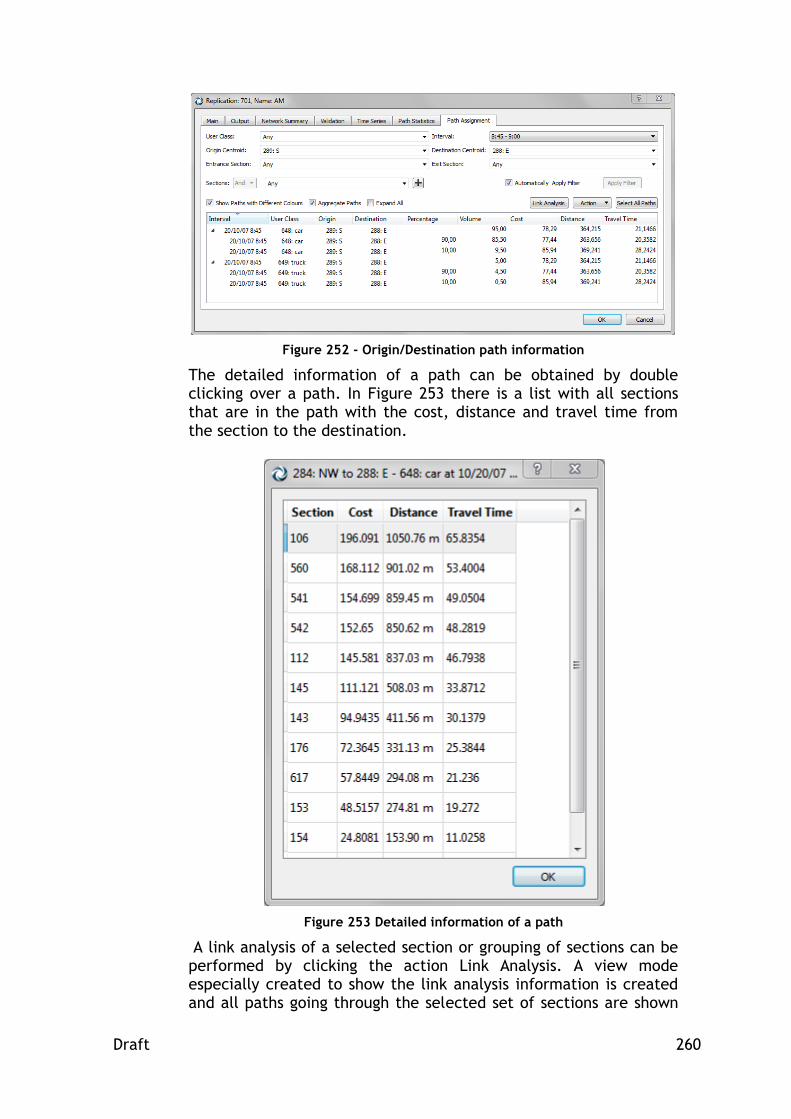
Draft 260
Figure 252 - Origin/Destination path information
The detailed information of a path can be obtained by double clicking over a path. In Figure 253 there is a list with all sections that are in the path with the cost, distance and travel time from the section to the destination.
Figure 253 Detailed information of a path
A link analysis of a selected section or grouping of sections can be performed by clicking the action Link Analysis. A view mode especially created to show the link analysis information is created and all paths going through the selected set of sections are shown

Draft 261
with the respective volumes. In there is an example of a link analysis. In Figure 254 there is an example of a link analysis where one section is selected.
Figure 254 Link Analysis
There are other options that can be performed:
Create Routes from selected paths. This option creates OD
Routes from the selected set of paths.
Output Matrices. This option creates the skim matrices using
the current filter values. There are four basic output skim
matrices: trips, cost, distance and travel time. In addition,
for the static assignment, also the matrices corresponding to
the Function Components defined will be calculated. In
Figure 255 the trips output matrix for all intervals and O/D
pairs is depicted.

Draft 262
Figure 255 Trips skim matrix
37.1.2 Path Statistics
While the Path Assignment tool can be used to study the assignment process and only those paths that were calculated by the route choice process are displayed, in the Path Statistics tab all used paths (user defined routes, user defined shortest path trees and route choice paths) are displayed. For each path the following information is displayed: (by checking the deviation toggle button the deviation is shown)
Origin Centroid. This is the origin centroid identifier.
Destination Centroid. This is the destination centroid identifier.
Type: RC (Calculated by the Route Choice process), UDR (User Defined routes), UDSPT (User Defined Shortest Path Tree).
Vehicles Assigned: Number of assigned vehicles to the path during a specific time interval.
% of Vehicles Assigned. The percentage of assigned vehicles that use the path for a selected origin/destination. Any vehicle that enters into the networks is counted as assigned.
Vehicles Entered. Number of vehicles that were assigned to this path at a specific time interval and were able to follow the path completely during the simulation time. (They finished the path.)

Draft 263
Travel Time (Entrance) Mean. The mean travel time path for all vehicles that used the path and start the simulation during a specific interval time.
Vehicles Exited. Number of vehicles that exited the path during a specific time interval.
Travel Time (Exit) Mean. The mean travel time path for all vehicles that used the path and exit the simulation during a specific interval time.
In Figure 256 there is an example of an O/D pair with all used paths. Notice that one of them is a user defined route. As can be done in the Path Assignment editor the user can display more than one path at the same time. These paths are coloured with different colours.
Figure 256 Path Statistics window
Another graphical visualization that can be obtained in this page, more suited for link analysis is available when a section, a list of sections or a group of sections is selected. By checking the Link Analysis checkbox, the view mode is switched to one where all the paths in the list are coloured in red and the width of the bars on the sections with volumes is proportional to the volume on them.

Draft 264
Figure 257 Link Analysis for one section
The View Styles included in the Link Analysis View Mode are:
A style for the width of each section, proportional to its
volume.
A style for the colour: used sections are painted in red.
A style for the label of the assigned volumes on the sections.
Two styles to hide section objects and nodes.
37.1.3 En-Route Path Assignment Information
When a vehicle decides to make a reassignment of the path during its trip, the decision is taken using probabilities calculated by the Route Choice model. En-Route Path Assignment dialog is located in the replication editor in the same way as the path assignment and path statistics editor. It is always accessed via the destination centroid. Consequently, a destination centroid must be selected first. This can be done either by selecting the centroid in the ‘Destination’ list or by clicking on it in the active 2D view. Once the destination centroid is selected, the next step is to select an origin section to obtain the particular path from that section to the destination centroid. This can be done by selecting the section in the ‘Origin Section’ list or by clicking on it in the active 2D view. For the shortest path, a list of probabilities of all shortest paths per vehicle type and per exit section calculated by considering the route choice model is displayed as can be seen in Figure 258.

Draft 265
Figure 258 En-Route Path Assignment Information

Draft 266
38 Support for Multi-network Projects
Aimsun includes the possibility to create revised networks from a base network as well as two open two different models at the same time. See the details in the following sub-sections.
38.1 Revisions
Network revisions arise from projects that start from an initial situation and want to study changes or event A revision is a network modification, which only stores those elements that have been changed editing the network1.
38.1.1 New Revision
To create a revision of your current network (we will call it base network) select Project/New Revision... and the following dialog will bring up:
Figure 259 New Revision Dialog
where,
Base Network: Base network name
Configuration Name: It is the suffix network name
New Initial ID: It is the starting Aimsun object ID for the new revision. By default, Aimsun calculates the value, but we strongly recommend to increase it in order to let future modifications in base network avoiding duplicate object IDs.
1 It's very important to define the project outputs database in base network before starting producing new revisions.

Draft 267
For example, in Figure 264, 30000 should be a reasonable value.
Network Revision File: Destination revision folder. Click Ok button and, automatically, Aimsun closes the base network and opens the new revision, so it is ready to start the modifications. Figure 260 shows the base and the revised networks.
Figure 260 Revision modifications
Once we've got the some revisions, it is possible to make changes on base network. Those changes will be applied when opening the revision network, unless they affect some modified elements in the revision (see Figure 261).
Figure 261 - Base to Revisions

Draft 268
The figure above shows that base network (leftmost image) has a couple of reserved lanes. When these changes are applied in revisions, those that affect to updated elements are discarded.
38.1.2 Consolidate Revision
A Revision needs the base network to load the whole network, as it only contains the modifications. It is possible to transform a revision into a full network by joining the base and the revision information in the same file. This can be done from Project/Consolidate Revision
38.2 Multi-model
Aimsun can now open two files at the same time. A separate view is created when you open two networks, as shown below:
Figure 262 Separate views for each network
The Project window shows which project is active. You make the project active simply by clicking on it.
Figure 263 Project Window opened networks

Draft 269
39 Columns
Columns contain data related to a type of object, as for example statistical data. Simulating a replication, reading a real data set, and executing a static assignment are examples of processes that generate columns. Examples of columns are: level of service of nodes during a simulation, observed counts for detectors, assigned volumes for sections, etc. These columns are created automatically, but there is a tool to manage them that allows the user to delete any undesired temporal columns. This feature is available at menu Tools/Data Analysis/Remove Columns.
Figure 264 Remove Columns Dialog
To make easier to find a specific group of columns in the list, a filter is available. The user can filter results by Type of object, Name of the column and type of storage (whether it is a Temporal Column or not). The Select All button selects all the columns in the current list, and the Delete button removes all the selected columns. The Don’t Remove Used Columns option prevents the deletion of columns that are currently used, even if they are checked to be deleted.

Draft 270
40 Advanced Aimsun 3D
Presently the editing is undertaken in a 2D view, but it is updated in real time in a 3D view. The main 3D features have been already introduced where applicable, but let’s see some of them in more detail.
40.1 3D Info Window
The 3D Info Window shows the library of textures and 3D models available for the network. It can be shown by accessing the Window Menu, Windows submenu, 3D Info option.
Figure 265 3D Info Window
There are three folders in this window:
The Vehicles folder: All the available 3DS files to be used as vehicles in the 3D views will be shown.
The Shapes folder: All the available 3DS files to be used as shapes, that is, decoration, in the 3D views will be shown.
The Textures folder: All the available image files to be used in the 3D views will be shown.
40.1.1 Vehicles folder
Any simulation can be presented in a 2D View and/or in a 3D View. In 3D views, the simulation vehicles use a 3DS shape to be visualized. Refer to the Vehicle Type Editor section for details on associating 3DS shapes to vehicles.

Draft 271
Figure 266 3D Info Window’s Vehicles Folder
The 3DS shapes that will be shown in this folder must be located in the <AIMSUN_HOME>/shapes/cars or in the <network folder>/shapes/cars folder. The AIMSUN_HOME folder is the folder where Aimsun is installed and the network folder is the folder where the current .ang file is located. There is a group of 3DS shapes available with the Aimsun installation. However, the user can use its own 3DS files by just copying them into the folders already explained. When double-clicking on a vehicle shape in the vehicles folder, the Vehicle's 3D Shape Editor will appear. There, all the shape parameters can be defined. See the Vehicle's 3D Shape Editor section for more details.
40.1.2 Shapes folder
The shapes used in 3D views as decoration objects will be shown here. In order to use any 3DS file as shape they need to be located either in the <AIMSUN_HOME>/shapes folder or in the <network folder>/shapes folder.

Draft 272
Figure 267 3D Info Window’s Shapes Folder
As it happens with the 3DS used for vehicles, the user can use their own 3DS files just copying them into the folders already explained. When double-clicking on a shape in the Shapes folder, the 3D Shape Editor will appear. There, all the shape parameters can be defined. See the 3D Shape Editor section for more details.
40.1.3 Textures folder
The textures that can be used in 3D views will be shown here. Image formats available to be used as textures are jpg, png, tga, and gif files.
Figure 268 3D Info Window’s Textures Folder
The images to be used as textures must be located in the <AIMSUN_HOME>/shapes/textures folder or in the <network folder>/shapes/textures folder.

Draft 273
Textures can be applied to the sky and floor, to polygons, to blocks (or extruded polygons) and to 3D Images. When double-clicking on a texture in the Textures folder the Texture Editor will appear. There, all the texture parameters can be defined. See the Texture Editor section for more details.
40.2 Vehicle's 3D Shape Editor
The Vehicle's 3D Shape editor can be opened by double-clicking on a 3DS Shape in the Vehicles folder in the 3D Info Window. It is used to select the different colour sets that the 3DS shape will be drawn with, as well as to define its dimensions, its rotations, the camera displacement of the cameras that will be located inside it and its animation parameters if any (see Figure 269). It also has an online visualization of the shape with the current colour set definition.
Figure 269 Vehicle's 3D Shape Editor

Draft 274
40.2.1 Colour definition
Any number of colour sets can be defined for a vehicle shape. The only requirement is that the colour sets percentages must sum up 100. To define a new colour set, the Add button must be pressed. This action will add a new line in the Set/Percentage column and a list of random colours associated to each of the parts of the vehicle shape in the columns <Material, Colour>. The colour associated to each material (or part) has three components, Ambient, Diffuse and Specular, which can be changed by clicking on the corresponding coloured square. A colour editor will appear. To remove any undesired colour set, select it and press the Remove button. To change the name of the colour set, double-click on the current name and, when it becomes editable, type the new name. To change the percentage assigned to the colour set, double-click on the current percentage and, when it becomes editable, type the new percentage. While defining the colour sets for a vehicle shape, the Automatic Percentages button can be checked to equally distribute all the colour sets’ percentages. Figure 270 displays three different colours for the same vehicle shape.
Figure 270 Definition of different colours for the same vehicle shape
40.2.2 Vehicle Shape rotations
To draw the vehicles correctly while simulating, the shapes associated to them must be rotated correctly, that is, in the picture of the vehicle shown in this dialog:
- its front must face to the right of the dialog. - its upper part must face up.
The following figure displays a shape before rotating it and the same shape correctly rotated with its rotations defined.

Draft 275
Figure 271 Vehicle Shape Rotations
These rotations are expressed in degrees and they can be set using the Shape rotations part of the dialog
40.2.3 Vehicle Shape dimensions
In the Dimensions dialog section, the real length, width and height of the shape can be defined. These dimensions are used to scale a vehicle proportionally with a different length than the one specified here.
40.2.4 Camera displacement
During the simulation, if the user clicks on a vehicle, a camera is placed inside it to allow the user to follow its movement along the network as the vehicle’s driver. The values defined here are used to locate the camera inside the vehicle. The origin point (with coordinates (0.0, 0.0, 0.0)) is the middle upper front point (see Figure 272). The x coordinate is the distance the camera will move from the origin point towards the back of the vehicle. The y coordinate is the distance the camera will move towards the left of the vehicle (the left supposing that the user is inside it). The z coordinate is the distance the camera will move from the upper part of the vehicle towards the bottom.
Figure 272 Camera Displacement

Draft 276
40.2.5 Shape animation
A 3DS shape can have more than one frame to represent movement. If a shape has frames to animate, these can be used in the simulation. The properties found in this group define the shape animation (see Figure 273).
Figure 273 Shape Animation Properties
A 3DS shape may have one frame that represents the stop position, another one that represents the starting movement and several more that make the movement loop. Our convention is that the stop frame, if any, is the first frame; the start frame, if any, is the following frame; and finally the rest of frames define the movement. Then, the properties that can be defined are:
Use animation: when selected, all the frames will be used in loops during the simulation and when not selected, only the first one will be used.
: when this button is pressed, the animation can be seen in the bottom right section of the Shapes Dialog. In this
case, its shape changes to . When the button is pressed, the animation is stopped.
Use Stopped Frame: when selected, the first frame will be considered as the stop frame so it will only be used when the vehicle is stopped, that is, the movement loop will not use it.
: when this button, next to the Stop or to the Start Frame, is pressed, the frame can be seen in the bottom right green square of the Dialog.
Use Start Frame: when selected, the second frame will be used whenever the vehicle needs to start its movement, that is, the movement loop will not use it.
Distance: here the user sets the distance that the shape will cover when moving from the first animation frame to the last one.

Draft 277
40.3 Vehicle editor’s 3D Shapes folder
In the vehicle editor in the Project Window, Vehicle Types and Classes folder, there is a folder in which to define the 3DS shapes that will be used in 3D views to draw all the simulation vehicles that belong to the edited vehicle type.
Figure 274 Vehicle’s 3D Shapes Folder
The Calculate % is a utility that distributes the shapes equally in each interval, saving users the work of inputting all the data if merely a uniform distribution is required. The Always vertical tick sets the shapes as to keep their vertical line when moving on slopes. This option should be ticked for pedestrians to make their movement realistic when going up or down stairs but should be unticked for road vehicles to make them look correctly when they go through sloped sections. Two examples for editing non-articulated and articulated vehicle’s 3D Shapes follow.

Draft 278
40.3.1 Non-articulated vehicles
In the case of a vehicle type called car, whose minimum and maximum lengths are 3 and 6 meters, the user could, for example, press the Add button six times to generate six different cases.
Each row in the list defines a 3DS shape that will be used in a sub-interval of the vehicle’s minimum and maximum length in a certain percentage. The interval’s initial length (called from), the interval’s final length (called to) and the percentage parameters can be changed by clicking on any of them and typing the new value. The 3DS shape can be changed by selecting the desired one in the list of available shapes that appears when clicking on the current shape. The percentage must be a value between 0 and 100.
The following image shows that vehicles between 3 and 4 meters will use the shapes s3 and sei with a probability of 50% each. Those between 4 and 5 meters will use the shapes 4x4, bora and pickup with probabilities 33%, 33%, 34% respectively, and all vehicles between 5 and 6 meters will all use the shape espace_2909.
Figure 275 Definition of 3D Shapes for a vehicle
When a new shape is selected, it is drawn in the green square on the bottom right (see Figure 274). In the green square, the mouse can be used to rotate or zoom in and out on the vehicle being previewed. Clicking without releasing the left mouse button and moving the mouse up, down, left or right rotates the vehicle. Clicking without releasing the right mouse button and moving the mouse up/down zooms in and out on the vehicle.
40.3.2 Articulated vehicles
An articulated vehicle is a vehicle that has a set of shapes connected one after the other (see the example in Figure 276). To define a vehicle as articulated, please refer to Vehicle Type Editor section.

Draft 279
Figure 276 Example of an articulated vehicle
When clicking the Add button for an articulated vehicle, a new vehicle shape interval is added where the user can change the initial and end length of the interval and the percentage (a value between 0 and 100). In the articulated Properties part of the editor, the shape for each part of the articulated vehicle can be selected.
As it happens when the vehicle is not articulated, the current 3DS shape selected is drawn in the green square and it can be rotated and zoomed using the mouse.
Figure 277 shows the dialog when the shapes of an articulated vehicle type have been defined.
Figure 277 Shapes definition for an articulated vehicle type
40.4 3D Shape Editor
The 3D Shape editor can be opened by double-clicking on a 3DS Shape in the Shapes folder in the 3D Info Window. It is used to define the dimensions the 3DS Shape will be drawn with in the views (see Figure 278).

Draft 280
Figure 278 3D Shape Editor
In this editor, the length, width and height defined in the 3DS file are shown. The user can decide whether to use these dimensions when adding a shape to the model or to define new ones. To do it, the Use Original Dimensions option must be checked or unchecked. When unchecked, a new length, width and height can be defined. These last values will be the initial dimensions of the shape when added to any model. Note that, once added, any shape can be rescaled using its own editor. Refer to the 3D Shape Object Editor section for more details.
40.5 3D Shape Objects
3D Shape objects are decoration objects that can be added to any model to add realism. To add a 3D Shape object, open the 3D info window, activate the Shapes folder, drag the desired 3D Shape among the available ones and drop it into a 2D view.

Draft 281
Figure 279 Drag and drop a 3D Shape to create a 3D shape object
Once the 3D Shape has been dropped, the 3D Shape object will be created. A 2D wireframe projection of the shape will appear in the 2D views and the realistic representation of the 3D Shape will appear in the 3D Views (see Figure 280).
Figure 280 3D Shape Object in a 2D view and in a 3D view
The 3D Shape object created will have the dimensions defined for the 3D Shape used. Refer to the section for details. To define new dimensions for this 3D Shape object different from the initial ones the 3D Shape Object editor can be opened by

Draft 282
double clicking on the 3D Shape Object. Refer to the 3D Shape Object Editor section for details.
40.6 3D Shape Object Editor
When double-clicking on a 3D Shape Object on a 2D or 3D View, the 3D Shape Object Editor appears.
Figure 281 3D Shape Object Editor
In this editor, the length, width and height of the 3D Shape object can be defined. When clicking on the OK button, the 3D Shape object will be rescaled in all views. A checkbox allows defining whether rendering in 2D will be a box or the 2D wireframe projection of the shape. There is also a slider that overrides the original “brightness” of the 3D model by adjusting its material’s properties. This is useful when your imported models, due to differences in lighting between different programs, appear darker or brighter than expected.
40.7 Texture Editor
When double-clicking on a Texture in the Textures folder of the 3D Info Window the Texture Editor appears.

Draft 283
Figure 282 Texture editor
Using this editor, a width and height for the texture can be defined. When a texture has a width and height defined and the Use Texture's Width and Height option is checked, then the texture will be scaled following these dimensions whenever applied into any object and it will be automatically replicated. If the Use Texture's Width and Height option is not checked then the texture will be scaled following the number of horizontal and vertical repetitions defined. Refer to the Polygon Editor and the Extruded Polygon Editor sections for more details.
40.8 3D Images
3D images are used to add objects, such as trees and traffic lights, to make the 3D views more realistic. To add a 3D Image, select the 3D Image tool and click on a 2D view. In a 2D View a 3D image is represented using a 2-point segment and a circle on it that indicates the face where the texture will be applied. This segment is going to become the ‘support’ of the 3D image.
Figure 283 3D Image Tool
Note that the 3D Image tool can be used in continuous mode (by double-clicking on the icon) to add as many 3D images as desired efficiently. A 3D Image is like a wall but without depth. These images have two main uses:
To add trees to the network. This option is very useful because the tga files can have a transparent area and then the trees are drawn efficiently (using a single polygon

Draft 284
instead of thousands) but realistically using the texture (See Figure 284).
Figure 284 Different trees representations used in 3D Views
To add any object (i.e.: advertisements) drawn in a tga or png file. This is especially useful when adding textures that have a transparent component. Figure 285 provides an example of drawing a realistic streetlamp using a tga texture.
Figure 285 Original TGA file vs. its representation in a 3D View
40.8.1 3D Image Editor
When double-clicking on a 3D Image the 3D image Editor appears.
Figure 286 3D Image Editor
In this editor, the image’s height as well as its texture can be defined. To define the texture click on the texture path button and select it. It also has a check box to set whether the image will

Draft 285
always face the camera or not. The image is placed on a rectangle and by selecting this option, the rectangle will rotate as the camera moves in order to be permanently facing the camera so that the face with the associated texture will be the only one seen. In Figure 287, three different positions of the image can be seen.
Figure 287 3D Image’s different positions
A 3D image has an altitude, that is, the Z at which the base of the image will be located. This altitude can be modified by selecting the image in a 2D View and with the Control key pressed dragging the mouse up or down. The current altitude will be shown while dragging. The width of a 3D image can be changed by editing the two segment points that represents it in 2D. Finally, a texture can be applied without using the editor by dragging the desired texture from the 3D Info Window to the 3D image in either a 2D or a 3D view.
40.9 Cameras
A camera sets up a point from which it will be possible to view the network and the 3D animation in the 3D viewer environment. The number of cameras that the user can create is not limited.
To add a new camera, select the Camera tool and click on a 2D view.
Figure 288 Camera Tool
In a 2D View a camera is represented using the following shape:

Draft 286
Figure 289 - 2D Camera representation
The camera head indicates where the camera is pointing. As with any graphical object, a camera can be translated by selecting it and dragging it in a 2D view to its new position. Using the Rotation
tool , selecting the camera and rotating it in a 2D view can change the aiming point.
40.9.1 Camera Editor
The camera editor will show the camera parameters. The editor pops up by double clicking on a camera in a 2D view and by pressing the Parameters button located in a 3D view (that will open the 3D view’s current camera editor).
Figure 290 Camera Editor
Using the editor, the camera can be renamed and its location parameters can be changed. To rename a camera its context menu can also be used. The parameters that define the camera location and where it is pointing to are:
Position: Point at which the camera is located.
Centre: Any point in the camera’s vision line.
VUp: Vector that defines the camera orientation in the plane perpendicular to the Position-Centre line.

Draft 287
Field of View: Changes the degrees of the angular extend of the view that is seen in any given moment.
Figure 291 Camera Parameters
40.9.2 Camera commands
In the View menu, there are three commands that apply to cameras:
Reset camera to place the camera in the active 3D view at its initial position, undoing all the rotations, translations and zooms that it may have undergone.
Set Camera parallel to floor to set the current camera in the active 3D view parallel to the floor’s surface. This option is particularly useful for fixing the camera’s position from any undesired rotations.
Set Camera perpendicular to floor to set the current camera in the active 3D view perpendicular to the floor’s surface.
40.9.3 Default cameras
When a 3D view is opened for the first time, if no cameras exist then four default cameras are created. These cameras are:
Main Camera: camera located at a default point from where the whole network can be seen. Translations and rotations are allowed.
Camera fixed X: fixed camera with the view line parallel to the X-axis; only translations are allowed.
Camera fixed Y: fixed camera with the view line parallel to the Y-axis; only translations are allowed.
Camera fixed Z: fixed camera with the view line parallel to the Z-axis; only translations are allowed. This camera is similar to the 2D views.
40.9.4 Camera Routes
A camera route is a group of camera positions that will be played and animated in 3D views. Refer to the Editing Dynamic Bookmarks for details on defining camera routes.

Draft 288
40.10 Selected objects in 3D views
Selected objects are drawn with extra red lines in 3D views to recognise them. See Figure 292.
Figure 292 - Selected object in a 2D and in a 3D View
40.11 Navigation in 3D views
To navigate in 3D views, the mouse and the keyboard can be used. If it is desired to use the mouse, then the appropriate icons in the View Commands tool bar must be selected previously.
Figure 293 Navigation tools
40.11.1 Selection tool
In 3D views, the selection tool is used to open the object editors (by double-clicking on the desired object) and to create and locate a camera inside a simulation vehicle during a simulation. This camera will be updated with the vehicle’s position at every simulation step. To do so, just single click on the desired vehicle. Whenever a vehicle with a camera inside leaves the network, the views that have the vehicle’s camera as the current one, change

Draft 289
back to the camera that was being used before the vehicle was selected.
40.11.2 Pan tool
The pan tool is used in 3D views to move the 3D view’s active camera to a new location. To move it over the 2D plane perpendicular to the view’s orientation, the left mouse button must pressed on any point of the graphic area, and without releasing it, move the mouse to the desired position (up, down, to the right or to the left). If the desired movement is forward/backward, press the Ctrl key, click and drag the mouse upwards/downwards to move the camera forward/backwards. Pressing the Shift key provides another function. Keeping the Shift key pressed, the first mouse movement determines the direction of movement. This means that, for instance, if the desired movement is upwards and any other displacement due to lateral mouse drifts is to be avoided, the way to proceed is to press the Shift key, click on the graphic area and drag the mouse upwards. Maintaining the Shift key pressed will also accelerate the displacement speed of the camera. That is, if the Shift key is hold pressed and the movement is maintained in the same direction:
moving the mouse
releasing the mouse’s button when the border of the application window is reached
moving the mouse to the graphic area again
pressing the mouse's left button and keeping it pressed
going back to step 1 the displacement speed will meanwhile also increase.
40.11.3 Camera rotation tool
The camera rotation mode allows the user to rotate the view’s active camera taking as the centre of rotation the position of the camera. To rotate the camera, the left mouse button must be pressed and, without releasing it, the mouse must be moved in the desired direction.
If the Ctrl key is pressed while moving the mouse, the camera moves forward or backwards as in translation mode.
The effect of pressing the Shift key is the same as in translation mode: it filters movement drifts and accelerates the rotation speed.

Draft 290
The rotation tool is not used in 3D Views.
40.11.4 Moving and rotating using the keyboard
As explained previously, the user can move and rotate a camera using the mouse. It is also possible to move and rotate it using the keyboard arrows and the control and shift keys. The main camera movements and rotations are movement forwards and backwards and rotation right or left. The arrows used to do this are as follows:
However, for all the movements and rotations to be accessible via the keyboard, the function of the arrows changes depending upon whether the ctrl or shift keys are pressed. When the Ctrl key is pressed, the arrow keys functions are:
Finally, when the shift key is pressed the arrow keys functions are:
These movements are valid for cameras that allow translations and rotations. When a camera only allows translations, the movements with the keyboard are only translations.

Draft 291
41 Quick reference guide to Aimsun Commands
Brief explanation of all the commands available using either the menu or the object’s context menu.
41.1 Menu commands
41.1.1 File Menu
New: opens a new empty network.
Open: opens an existing network.
Close: closes the current network.
Save: saves the currently open network.
Save as…: saves the currently open network, with the option to provide a new name.
Import: imports CAD files or other third-party software files depending on the components loaded as, for example, Emme networks or CONTRAM networks into the current Aimsun network.
Export: exports the current Aimsun network to several formats (as shapefiles, image files, Emme, …).
Print: prints the current 2D view.
Print Preview: opens the print preview window.
Export to PDF: saves the current 2D view in PDF format.
Recent Files: list of the last opened files for a fast access in case any of them is to be opened again.
Quit: exits the application.
41.1.2 Edit Menu
Undo: undoes last action.
Redo: redoes last action.
Cut: removes the selected objects and places them on the clipboard.
Copy: copies the selected objects to the clipboard.
Copy Snapshot: stores in the clipboard an image similar to the active 2D View.
Paste: copies from the clipboard to the center of the drawing area.
Paste at Original Location: copies from the clipboard to the drawing area keeping the original coordinates of the copied objects.
Clear: deletes the selected objects.
Select All: selects all the objects in the drawing area.
Inverse Selection: unselects all selected objects and selects all those that were not selected.
Find: opens an editor where to find objects that match the criteria.
Move Selection to View Centre: locates the selected objects in the centre of the view.

Draft 292
Models: show or hide parameters for Aimsun Macro and Travel Demand Modelling, Aimsun Meso and Aimsun Micro. Only visible when the edition is an Aimsun Advanced or Aimsun Expert.
Labels: customizes the font size of on view labels. Customizes also the content of the Show Label command (ID, name, external ID)
Preferences: opens the Preferences editor where to specify the overall parameters of the traffic network currently being edited if any or the overall system parameters otherwise.
41.1.3 View Menu
New 2D View: creates a new 2D View of the current network.
New 3D View: creates a new 3D View of the current network.
Close Current View: closes the active view.
Full Screen: Maximises the Aimsun application.
New Layer: adds an empty layer to the group of layers.
Set Time: opens a dialog where to set the view current time, the time interval that must be shown, the animation refreshing rate and parameters about the time series used in the view mode used.
Centre World: locates the whole network in the centre of the active 2D View.
Whole World: changes the zoom of the current 2D view to fit the whole network.
Max Zoom for Visible Car Detail: Adapts the 2D view zoom to allow the simulation vehicles visualisation.
Pan to...: opens a dialog to select the coordinates where to centre the view.
Pan to Object being edited: centres the view in the current edited object in a dialog.
Show Latitude and Longitude: toggles the display of coordinates as latitude and longitude instead of UTM coordinates.
Show Object Tooltips: Activates tooltips in 2D view objects.
Centroids: toggles whether to display the centroid polygon, centroid points and centroid connections in the views.
Supernodes: toggles whether to display supernodes and supernodes objects in the views.
Reset Camera: retrieves the initial parameters of the current camera in the active 3D view.
Set Camera Parallel To Floor: removes all the vertical rotations (pitch angle) of the current camera in the active 3D view.
Set Camera Perpendicular To Floor: changes the rotations of the current camera in the active 3D view to make it similar to a 2D View camera.

Draft 293
Show/Hide Dynamic Labels: shows or hides the dynamic labels defined in the currently open Aimsun networks.
Select Equal Dynamic Labels: selects all the dynamic labels that are defined as the one currently selected.
Close All Dynamic Labels: closes all the dynamic labels.
Close Selected Dynamic Labels: closes all the selected dynamic labels.
Close Equal Dynamic Labels: closes all the dynamic labels that are equal (showing the same attribute) as the selected one.
Quality: Defines the quality of the 2D visualization among Low, Medium or High.
Grey Mode: Visualizes the current 2D view with a white, black and grey aspect.
41.1.4 Arrange Menu
Group: groups the current selection of 2D objects in one
Ungroup: breaks an object.
Align Centres: translates the current selection to align the centre of all selected objects.
Change Altitude: changes the altitude of the selected objects.
Move to Layer…: moves the selected objects to the selected layer (i.e. Network, Network Layers…, Images, Images Layers…).
41.1.5 Project Menu
New…: creates Aimsun objects, in the current Aimsun project.
New Revision: creates a revision network of the current Aimsun project.
Consolidate Revision in Base: applies all the changes done in this revision to the base network and removes the link between the base and the revised networks.
Consolidate Revision in this Revision: converts the current open revision network into a base network removing the link between the base and the revised networks.
Revision Info: opens the properties of the current revision.
Properties: opens the properties of the current project.
41.1.6 Tools Menu
Public Transport Sections: opens the list of public transport sections available.
Check and Fix Network: checks the network for errors. If errors are found it opens an editor to fix the errors.
Set External IDs: sets external IDs automatically for objects of a given type.

Draft 294
Show Location in Google Maps: Opens a browser and loads into Google Maps the visible location (requires a network in UTM coordinates and a correct UTM Zone in the layers).
Import Turns from Shapefile
Import Nodes from Turns
Translate Selected Sections
41.1.7 Data Analysis Menu
New View Mode Wizard: opens a wizard dialog for creating view modes.
New View Style Wizard: opens a wizard dialog for creating view styles.
Time Series Viewer: opens the dialog for viewing Time Series.
Close All open Time Series Viewers: closes all opened time series viewers.
Delete Temporary Columns: opens the dialog for removing existing columns in the model.
Space Time Diagram: shows a space-time diagram of a selection of detector.
Data Comparison: opens the dialog for comparing two different experiments or sets of data.
Decision Table:
Shortest Path Calculator: opens the shortest path viewer tool.
Isochrones: opens the isochrones dialog.
41.1.8 Bookmarks Menu
Bookmark this Position: adds the current network view position and scale to the list of existing bookmarks.
Edit: opens and editor for editing existing bookmarks.
List of existing bookmarks: list of previously added bookmarks.
41.1.9 Window Menu
Windows: lets the user define which windows are visible or not. If the window is currently visible, a check mark will appear next to the name in the menu.
Tools Toolbar: lets the user define which toolbars are visible or not. If the toolbar is currently visible, a check mark will appear next to its name in the menu.
Welcome: displays the Welcome Widget to be able to open a second model.
41.1.10 Help Menu
Manuals: opens a window with the selected users manual.
Licenses…: opens a window containing a list of all the licences modules, their expiration date and SUS information.

Draft 295
About: opens the Aimsun intro window.
About Plug-ins: for the selected component opens its intro window if any.
41.2 Graphical objects’ context menus
The context menu of any graphical object is opened by right clicking on the desired object in a 2D View. For all the graphical objects there are several common operations accessible opening their context menu. These commands are:
Show Label: shows in the 2D views the labels “identifier: name” for all the objects belonging to the same type as the type of the object owning the opened context menu.
Dynamic Labels: o New:
Attribute Dynamic Label: Opens a dialog where to select the attribute the dynamic label in the 2D views will be based on.
o Select Equal: Selects all the dynamic labels that are equal to the one displayed for the object right-clicked.
o Close: All: Closes all the current visible dynamic labels Selected: Closes all the selected dynamic labels Equal: Closes all the dynamic labels that are
showing the same attribute, but for other objects, as the one that open the context menu.
Rename: opens a window where the object can be renamed.
Delete: deletes the object.
Properties: opens the object editor.
Arrange: o Group: groups the current selected objects all
together. o Align Centres: translates the current selected objects
to make their central point be located at the same place.
o Change Altitude: changes the object's altitude, that is, places its bottom part where indicated.
o Move to Layer: moves the selected objects to the selected layer (i.e. Network, Network Layers…, Images, Images Layers…).
Generate Pedestrian Obstacle: generates a pedestrian obstacle for Legion for Aimsun with the object’s shape.
For each graphical object its operations are:
41.2.1 Polyline
Convert to Section: converts the polyline to a section.

Draft 296
Convert to Polygon: converts the polyline to a polygon by adding the line that joins the first and last point.
Extrude: converts the polyline to a 3D polyline.
Join: joins two selected polylines.
41.2.2 Bezier Curve
Convert to Section: converts the Bezier curve to a section.
Convert to Polygon: converts the Bezier curve to a polygon by adding the line that joins the first and last point.
41.2.3 Polygon
Select objects inside: selects in the 2D view all the objects that have some part inside the polygon.
Convert to: converts the polygon into a grouping, subnetwork or microsimulation area.
Extrude: converts the polygon to a 3D block.
41.2.4 Section
Change Section Direction: changes the direction of the section to the opposite direction.
Generate Opposite Direction: creates a new section next to the current section with the opposite direction.
Add curve vertex: adds a curve vertex to the section.
Join: joins the selected sections.
Speed…: opens a dialog to select the new speed for all the selected sections.
Capacity…: opens a dialog to select the new capacity for all the selected sections.
Lane Width…: opens a dialog to select the new lane width for all the selected sections.
Road Type: changes the road type of the selected sections updating the section attributes to the ones defined in the road type.
Road Type (Keeping Attributes): changes the road type of the selected sections without updating the other attributes of the section.
Number of lanes: changes the number of lanes of the selected sections.
Lane Type: changes the type of the clicked lane.
Convert to Polygon: converts the section to a polygon by adding the line that joins the first and last point.
41.2.5 Node
Edit Control Plan: All the defined control plans will be listed to select the one to be edited.
Yellow Box: the node will be considered as a yellow box node when checked and as a normal node otherwise.

Draft 297
Curve Turns: curves all the turns in the node changing the geometry of each one of them.
Show/Hide Turns Label: shows or hides in the 2D views the labels “identifier: name” for all the turns belonging to the node that opened the context menu.
Merge: merges the selected nodes into one.
Split: splits the selected node in several nodes, one being each one of the polygons the original node had.
Advanced Editor: Opens the advanced node editor where to see the connections and conflicts that will be used in the microsimulation. Refer to the Aimsun Dynamic Simulators Users’ Manual for more details.
41.2.6 Centroid
Join Centroids: When two centroids are selected, this option will join all their connections into one centroid updating the O/D matrices and O/D routes accordingly.
Edit Polygon: draws the points that define the centroid polygon to be able to edit it.
Hide/Show Connections: hides or shows the connections of the selected centroids with the sections or nodes.
41.2.7 Controller
Hide/Show Connections: hides or shows the connections of the selected controllers with the nodes.
41.2.8 Subnetwork
Generate Static Traversal: Refer to the Aimsun Macroscopic Modelling Tools Manual for details.
Generate Dynamic Traversal: Refer to the Aimsun Dynamic Simulators Users’ Manual for details.
New… o Scenario: creates a new scenario, either dynamic or
macro, for the subnetwork. o Traffic Demand: creates a new traffic demand for the
subnetwork. o Centroids Configuration: creates a new centroid
configuration for the subnetwork. o Traffic State: creates a new traffic state for the
subnetwork.
Select objects inside: selects in the 2D view all the objects that have some part inside the subnetwork.
41.3 Non Graphical objects’ context menus
The context menu of any non-graphical object is opened by right clicking on the desired object in the Project Window.

Draft 298
For all the non-graphical objects there are several common operations accessible opening their context menu. These commands are:
Rename: opens a window where the object can be renamed.
Delete: deletes the object.
Properties: opens the object editor. For each non-graphical object the rest of its operations, if any, are:
41.3.1 Road Type
Set As default: sets the road type as default. It means that from this instant all sections will be created using this road type.
41.3.2 Centroid Configuration
New: o O/D matrix: creates a new matrix in the selected
centroid configuration. o O/D route: creates a new route in the selected
centroid configuration.
Activate: sets the centroid configuration as the active one.
41.3.3 Dynamic Scenario
New Experiment: creates a new experiment in the selected scenario.
41.3.4 Dynamic Experiment
New o Replication: opens an editor for creating replications
in the experiment. o Average: creates a new average in the experiment for
a set of replications.
41.3.5 Replication
Animated Simulation: starts an interactive simulation. It opens the interactive simulation editor, which lets the user start the simulation, define the simulation speed and a simulation stop time.
Animated Simulation (Quick start): starts an interactive simulation. It opens the interactive simulation editor, which lets the user define the simulation speed and a simulation stop time. After the warm-up the simulation is automatically started.
Batch Simulation: starts a batch simulation.
Save Simulation State:
Retrieve Replication Data: loads the replication data that was stored into the database.
Retrieve Path Assignment Results:

Draft 299
Retrieve Path Costs:
41.3.6 Average
Calculate: calculates the average of the chosen set of replications. If a database is set in the scenario, it stores the average in the database too.
Simulate Pending Replications: simulates those replications with status set as ‘Not simulated yet’.
Reset Replications: Sets the status of all the replications that belong to this average to ‘Not simulated yet’.
Retrieve Average Data: loads the average data that was stored into the database.
Retrieve Average and Replications Data: loads the average data that was stored into the database as well as the data for all the replications belonging to it.
41.3.7 Public Transport Line
Select Route Sections: selects those sections that belong to the public transport line.
41.3.8 Strategy
New Policy: creates a new policy for the selected strategy.
41.3.9 Policy
New: o Lane closure: creates a new lane closure action for
the selected policy. o Turn closure: creates a new turn closure action for
the selected policy. o Speed change: creates a new speed change action for
the selected policy. o Force turn: creates a new force turn action for the
selected policy. o Rerouting: creates a new rerouting action for the
selected policy. o Section incident: creates a new section incident
action for the selected policy. o Periodic Section incident: creates a new periodic
section incident action for the selected policy. o Control plan change: creates a new control plan
change action for the selected policy. o Meso Behavioural Parameters Change: o Deactivate Reserved Lane:
41.3.10 Traffic Condition
New: o Lane closure: creates a new lane closure action for
the selected traffic condition.

Draft 300
o Turn closure: creates a new turn closure action for the selected policy.
o Speed change: creates a new speed change action for the selected traffic condition.
o Force turn: creates a new force turn action for the selected traffic condition.
o Rerouting: creates a new rerouting action for the selected traffic condition.
o Section incident: creates a new section incident action for the selected traffic condition.
o Periodic Section incident: creates a new periodic section incident action for the selected policy.
o Control plan change: creates a new control plan change action for the selected traffic condition.
o Meso Behavioural Parameters Change: o Deactivate Reserved Lane:
41.3.11 Python Script
Execute: executes the python script. Refer to the Aimsun Scripting Manual for details on defining scripts.
41.3.12 Real Data Set
Retrieve: retrieves the data of the selected real data set.
41.3.13 Grouping Category
New…: creates a new grouping.
Build: adds to the groupings linked to a polygon area the objects inside the polygon that belong to the Grouping Category Object Type.
Refresh Statistics: recalculates the statistics of all the groupings defined in the grouping category.
41.4 Layer context menu
The context menu of a layer is opened by right clicking on the desired layer in the Layers Window. The available operations for layers are:
Generate Pedestrian Obstacles: generates a pedestrian obstacle to be used with Legion for Aimsun for each one of the objects in the layer.
Retrieve External Data: retrieves the layer so all its contents can be accessible by the user.
Unload External Data: unloads the layer contents so they will be no longer accessible by the user and the amount of memory used by Aimsun will decrease.
New Layer: creates a new sublayer.
Activate: sets the layer as the active one so all the new created objects will be added to it.

Draft 301
Centre in View: centres the view on the centre point of the layer
Move Selection to this layer: Moves all the selected objects to this layer.
Select All: selects all the layer objects in the active 2D View.
Show All: shows all the layer objects in the active 2D View.
Hide All: hides all the layer objects in the active 2D View.
Rename: opens a window where the layer may be renamed.
Remove: removes the layer.
Properties: opens the layer’s editor.
41.5 Legend context menu
Copy snapshot: copies the contents of the legend to the clipboard.
41.6 Log Window context menu
Save Log: Saves the log messages into an html file.
Clear: clears the log window by removing all of its contents.
41.7 Project Folders context menus
Right clicking on root folders within the Project window reveals their context menus. Apart from the Rename option available to all folders, new non-graphical objects relevant to each folder may be created. For example, a New / Vehicle Type may be created from the Vehicle Types and Classes folder’s context menu, which will be placed in this folder.
41.8 Hotkeys list
The hotkeys currently implemented inside the Aimsun application are:
F5 : Selection
F6 : Pan
F7 : Zoom
Control + R : Rotation
F9 : Connection
L : Layers Windows
P : Project Window
E : Legend Window
O : Log Window
T : Table View Window
I : Inspector
F2 : Rename.
F11 : Decrease current editor's opacity.
F12 : Increase current editor's opacity.

Draft 302
ESC : Closes current editor.
Ctrl+Q : Quit Aimsun.
Ctrl+G : Group the selection.
Ctrl+U : Ungroup the selection.
Ctrl+F11 : Maximizes the app (returns to the original size when
clicked again).
Ctrl+P : Print.
Ctrl+M : Joins the two selected sections
Ctrl+Number : when a section is selected changes the number of
lanes. Without a section selected changes the default number of
lanes for the future sections that will be created.
When an object is selected, the arrows move it.
When the pan tool is selected, the arrows move the view.

Draft 303
42 Aimsun scripting
42.1 Scripting
Python scripting is ideal for writing small utilities to automate some operations that would be done manually with the GUI. Typical tasks that might be performed with scripting are:
Modifying the model
Importing or exporting data
Performing calculations with the data of the model
Modifying the meta data model A prerequisite to using the scripting capabilities of Aimsun is some knowledge of how to program in Python (something not covered in this manual), and with this background the users can introduce themselves to classes and methods within Aimsun, and the conventions of their use. There’s a specific manual for scripting (Aimsun Scripting Manual) which includes examples that will introduce the reader to the effective use of scripting. It will also explain the conventions of use: what is it allowed, what is it not allowed and what it is the best way to do common tasks. The documentation of all the Aimsun classes and methods available in scripting is provided as a collection of browsable HTML documents (TSS-Transport Simulation Systems\Aimsun 7.0\programming\scripting\docs\index.html).
42.1.1 Creating a Python Script
Python Scripts can be created from Project/New/Python Script menu.
Figure 294 New Python Script
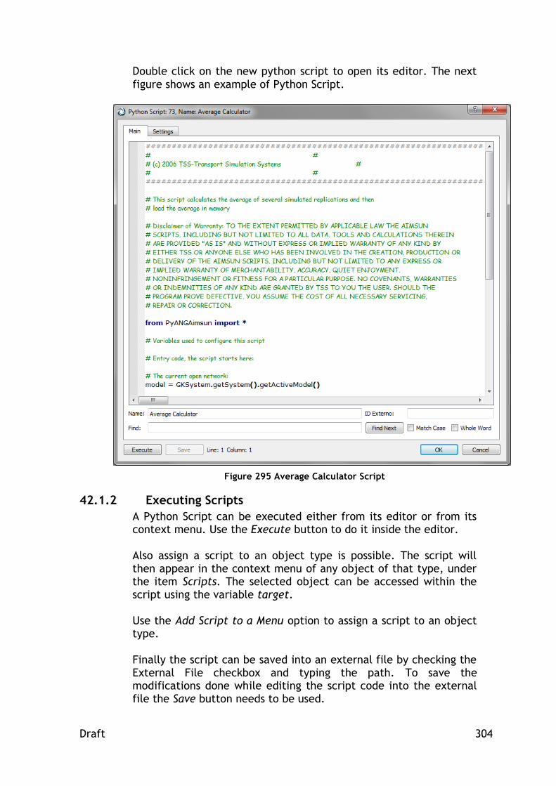
Draft 304
Double click on the new python script to open its editor. The next figure shows an example of Python Script.
Figure 295 Average Calculator Script
42.1.2 Executing Scripts
A Python Script can be executed either from its editor or from its context menu. Use the Execute button to do it inside the editor. Also assign a script to an object type is possible. The script will then appear in the context menu of any object of that type, under the item Scripts. The selected object can be accessed within the script using the variable target. Use the Add Script to a Menu option to assign a script to an object type. Finally the script can be saved into an external file by checking the External File checkbox and typing the path. To save the modifications done while editing the script code into the external file the Save button needs to be used.

Draft 305
Figure 296 - Assigning a script to Sections
For example, the script to print the ID of the selected object is:
print target.getId()
42.1.2.1 Automatic Initializations
The scripting environment in Aimsun is initialized executing the script initial.py located in the folder TSS-Transport Simulation Systems\Aimsun 7.0\shared\scripts\model\. It imports the following Python modules that contain the fundamental Aimsun classes required for model editing:
PyANGBasic: Qt classes
PyANGKernel: Aimsun Kernel classes
PyANGGui: Aimsun GUI classes In order to use the capabilities offered by the plug-ins, it is required to import the related modules. For example, to launch a Microscopic simulation within a script the PyANGAimsun module must be imported
from PyANGAimsun import *
Then, redirects the standard output to Aimsun Log window. Finally, it preinitializes the following variables:
model: contains the current network model
target: contains the object from which the script is executed, if the script is linked to an object type (see Figure 296)
selection: contains the objects currently selected

Draft 306
43 GIS Importer/Exporter
The objective of this plug-in is to load GIS files (ESRI Shapefiles or MapInfo Files) into Aimsun and to extract as much information as possible from it to create a transportation network. Using this tool is possible to create networks from several sources as Navteq or TeleAtlas maps or from other transportation packages as Cube, TransCAD or any other that can export its network data into GIS files. It also allows the export of certain information from the network geometry to shapefiles.
43.1 GIS importer
The importer can put the data in Aimsun in two different ways: 1. As Aimsun objects stored in the ANG file. 2. As an external layer
43.1.1 Importing in the Aimsun file
Aimsun stores all the network information in a single binary file with the ANG extension. When importing data from another format it creates Aimsun objects that are stored in such file. The GIS file will no longer be used.
43.1.2 Importing as an External Layer
For some file formats (CAD, GIS, Raster Images) it is possible to store not the contents of the imported data but a pointer to the file where the data was imported from. In this case, some part of the information will reside in the Aimsun file and some part will be on external files in its original format.
Figure 297 External Data on Aimsun

Draft 307
Aimsun uses external layers to know when the data in a drawing layer comes from an external source. This kind of layer, on document retrieval, reads the external data and incorporates it into the Aimsun model (if the Auto Retrieve is active, otherwise the user can load the data at any moment using the Retrieve command). On document save, only the location of the external file will be stored. Data in an external layer cannot be edited in Aimsun.
43.2 Shapefile Introduction
The Shapefile spatial data format is open and published by ESRI. Shapefiles store non-topological geometry and attribute information for the spatial features in a data set. Shapefiles can support point, line, and area features. The shapefile concept includes as many as five file types with specific file extensions. These files should be stored in the same workspace2. Shapefile file extensions and their function: 1. .shp: the feature geometry. 2. .shx: an index to the feature geometry. 3. .dbf: the associated dBASE file of attribute information. 4. .sbn and .sbx: a spatial index of the features. 5. .ain and .aih: the attribute index of active fields in a table or a
theme’s attribute table. When the user imports a shapefile to create data in the Aimsun file the importer will use the feature geometry (shp) to create one object for each object found in the shapefile. It will then use the attribute information to set the Aimsun object attributes. For example: if the user chooses to create a network from a shapefile the importer will create a section for each object in shapefile. The geometry (must be either a line or polyline) will be used as the centre line of each section. The attribute information will be used to set the number of lanes, capacity, road type, etc.
43.3 GIS File Units
Aimsun uses the metric system internally. When importing a GIS file, its coordinates are transformed to metres if they are in feet or latitude and longitude. In the second case, a conversion to WGS84 UTM coordinates is used.
2 http://www.uky.edu/KGS/mapping/pages/glossary.html

Draft 308
43.4 Data Requirements
The amount and quality of the data found in the GIS file will determine the quality of the imported data. If no number of lanes information is present, the importer will create single lane sections, if no speed information is found a default speed will be set (using the active road type) and so on.
43.5 Network Creation
Usually GIS data does not contain detailed geometry information of a traffic network. The missing information can be:
On ramp or off ramp information: A section contains only the main lanes or, if the on/off ramp is included, it is coded as a full lane.
Space for the nodes: a node is coded as a point instead of as an area.
Turn information: The section connectivity, if present, only codes “all to all” lanes turns (instead of, for example, only left most lane is used to turn to section Y from section X).
The importer will automatically create the node area based on the in and out sections geometry and will do its best to create the correct turn information. No on or off ramp will be created. However, the importer can be enhanced to extract non-standard information, see Customization Services.
43.5.1 Customization Services
The main objective of the importer is to create a network with the highest quality and amount of information. If the information is coded in a format not supported by Aimsun, or if extra data can be extracted from other sources of information then TSS offers customization services to enhance the importer. These services include modification of the importer logic (to add implicit rules) and the inclusion of interfaces to other data sources (such as Access or Excel files, spatial databases and files in custom data formats).
43.6 Importing a GIS File
This initial dialog asks for the importing process to use (create an external layer, create the network geometry and topology, create detectors or centroids or VMS, create buildings), the units and locale and the attributes in the GIS file to use as name and external IDs of the created objects.
1. Start Aimsun. 2. Create a new document using a template. 3. From the File menu, execute the Import / GIS command. 4. Locate the GIS file to import 5. The GIS Importer dialog appears:

Draft 309
Figure 298 GIS Importer Dialog
6. The type name is used to assign a type to each object imported. The type name must refer either to a type that doesn’t exist or to the name of an already existing type that can be used by the objects that will be imported. For more information, see the point Types and Objects in Aimsun below.
7. Set the correct units. The importer will try to guess the correct value.
8. If you are importing data in a language not covered by the ASCII character set (as Chinese, Japanese…) set the correct Encoding.
9. Set the attribute in the shape file to be used as the external identifier. Aimsun will put its own identifier on each imported object. The external identifier is also used to keep the identifier used in the shape file.
10. Set the attribute to be used as the name of each object. 11. Set how Aimsun will import the file:
As an External Layer: the file is imported as it is, no modification is carried out and no data is created in the Aimsun file. Only the path to the GIS file is stored. When

Draft 310
the user retrieves an Aimsun file that contains an external layer it will load the data from this GIS file.
As an Internal Layer: the file is converted into lines and points. After the conversion, the original file will no longer be used. The created objects will be stored in the Aimsun file.
As a Network: the file will be converted into an Aimsun network. After the conversion, the original file will no longer be used. The created objects will be stored in the Aimsun file. A dialog asking for extra information will appear.
As Centroids, VMS, Detectors or Bus Stops: the file will be used to create the selected Aimsun objects (centroids, VMS, detectors or public transport stops). After the conversion, the file will not be used. The created objects will be stored in the Aimsun file.
As Buildings: For each polygon on the file, an extruded polygon with the selected height will be created. The height can be either random, fixed, or can come from one of the attributes of the objects.
12. The imported objects will be placed in a new layer whose name will be the name of the used type.
43.7 Network Importer
The network importer will extract as much information as possible from a GIS file to create an Aimsun network. See How the Network Importer Works for a detailed description. Only GIS files that contain lines or polylines can be used to create a network. The importer will not work with polygons, arcs, points or multi-patch files. The dialog will ask for information about the sections (in the Main tab folder), how to connect these sections (Topology tab folder), whether the links include Centroid Connections (Centroids tab folder) and whether any attribute can be used to assign VDFs to the sections. The attributes number of lanes, speed and capacity can have two values, for the normal direction and for opposite directions in the case that a single link generates both directions.
43.7.1 Road Types
Before importing, the user can create as many road types as desired, which will be used to initialize values in the section when it is created.

Draft 311
Figure 299 Road Type Editor
When the network importer creates the sections on the network it is possible to use an attribute in the shapefile to specify the road type to be used. If no equivalence is defined, the new sections will have the default road type (as designed by the user using the Set as Default command in the Road Type context menu). If no value or attribute correspondence is specified in the network importer dialog for a particular section attribute then the importer will use, if possible, the values found in the road type. If the user wants to set the values from the road type instead, this can be done by setting the following values in the importer:
Speed: Select None
Capacity: Select None
Lane Width: Leave the field blank.
43.8 How the Network Importer Works
The network importer will create a section for each polyline found in the GIS file. Then it will create the nodes using the From Node and To Node attributes. Each node will contain all the possible turns between all the sections in that node. Then it will process each turn to remove the U-Turns and to fine-tune the lanes used in each turn. It will expand the nodes from a point to an area

Draft 312
(optional step). The last (optional) step will be the import of extra node information from another GIS file.
43.8.1 Section Creation
Each polyline or line found in the GIS file will be converted to a new section.
Figure 300 Network Importer Dialog: Sections
It is currently possible to specify, based on the attributes on the GIS file, values for number of lanes, speed and capacity. If no information is present for any of these attributes the following values will be used:
Attribute Value

Draft 313
Number of lanes 1
Speed Speed from Road Type
Capacity Capacity from Road Type
The road type can be set in the Network Importer dialog. If no road type is set then the default Road Type will be set. It is possible to add a number of lanes by road type if no attribute for number of lanes is specified in the Section Basic area. Note that Aimsun uses metric units internally. The imported GIS file will create sections in metres. If the GIS file units were metres then the geometry in the GIS file and the centre line of the sections will be the same (unless some post processing is applied such as making space for the nodes).
43.8.1.1 Links to Skip
Some GIS files can include links that maybe are not required, for example a metro or train line. It is possible to skip using the Road Type Attribute and setting a 0 as the number of lanes. In this case it is not required to assign an Aimsun Road Type.
43.8.1.2 Single and Dual Direction
Usually the polyline in the GIS file codes a centreline of a single section, and the order of the points in the polyline determines the direction of flow. However, the importer also supports the following alternatives:
Inverse sections: The direction of flow is the inverse of the point order.
Dual directions: The polyline codes the separation line between two sections, one in each direction. It is possible to combine both possibilities (inverse and dual).
Use the Direction of Flow area to tell the importer how to discover the right direction and if the polyline codes dual direction. To do so select the attribute that has the information and put for each possibility the number, character or text that identifies the correct setting. Put a non-valid entry if a setting is not possible. Example: a GIS file has an attribute named DIR with these possible values:
1: Single Direction
-1: Inversed Direction
0: Dual Direction So write 1, -1 and 0 for the three first possibilities. For the last possibility (Dual Direction Inversed) put anything that is not 1, -1 or 0.

Draft 314
43.8.1.3 Number of Lanes and Dual Direction
When a single polyline generates two sections, one in each direction, the number of lanes attribute found in the GIS file can be considered as the sum of all the lanes in both directions or as the number of lanes for each direction. Activate the toggle button Share Lanes in Dual Direction to divide the number of lanes between both sections.
43.8.1.4 Overlapped Sections
Some shapefiles contain two overlapped centrelines for each direction of flow. Figure 301 shows two links, 1 and 2, which connect two nodes, A and B. Aimsun can automatically move these overlapped centrelines to ensure a more correct network geometry.
Figure 301 Dual direction using two centerlines
This operation is activated by checking the Unoverlap Sections option. The application will look for pair of sections that connects opposite nodes (section 1 goes from A to B, section 2 from B to A) and will displace the sections outside the original centreline. The current Rule of the Road will be used (as set in Preferences) to determine which section will be translated to the left of the centreline and which one will be translated to the right.
43.8.2 Node Creation
If the GIS file contains topological information (in our case how objects are connected), it can be used to create nodes where sections on the network are connected. The “From Node” and “To Node” attributes are used to create such nodes.
A B
1
2

Draft 315
Figure 302 Network Importer Dialog: Nodes
After a node is created, turns on the node are also created to physically connect sections, to each other. As no information is available on which section is connected with which, the importer creates a connection between all the sections in the node.
43.8.2.1 Turn Refinement
Aimsun can specify not only which sections are connected to which sections in a node but also which lanes are used in a turn. For example, in a right turn, maybe only the rightmost lane of a section allows such a turn and the rest of the lanes are used to go straight ahead.

Draft 316
Figure 303 Example of a turn in Aimsun
The importer classifies the turns to determine if they are a u-turn, left, right or straight turn. It uses the angle that forms the sections that are connected before the node is expanded. After the turn angles have been calculated and the turns classified the importer will assign some or all of the lanes to the turn, considering other turns that start in the section, as follows:
Turn Type Other Turns on Sections
Lanes Used
Left Straight Left most
Left None All
Left Right Half (left most)
Right Straight Right most
Right None All
Right Left Half (right most)
Straight None All
43.8.2.2 Expanding the Node
The last step will convert the node from a point to an area giving space to the turns. It will compress the sections that are part of the node reducing each section. The compression will make the section shorter but neither section will be removed nor any point on it. The compression size will depend of the number of lanes of the sections involved. The importer will use the maximum size of the section width (number of lanes * lane size) divided by 2 and, to the result, it will add a 10%. This space will ensure a correct node area for most of the cases but it will not try to guarantee that some sections do not overlap the node.
43.8.2.3 Adding Extra Node Information
The user can specify a second GIS file with node information. The importer creates nodes based on the “From Node” and “To Node”

Draft 317
settings. Each node created will have as its external identifier the value of the “From Node” or “To Node” attribute. In order to use this second GIS file the importer must match the nodes created when importing the network with the nodes found in this shapefile. The importer will ask for the attribute that contains the identifier of the node. It will also ask for the attribute that contains the name of the node. No geometrical information will be loaded, only the attributes and its values.
43.8.3 Centroid Creation
Some GIS files contain centroid connections as links. In this case, Aimsun can automatically create the centroids and connect them to the corresponding section or node. In the Centroid tab folder, enable the Centroid connections in Links option and then tell the importer how it can recognize connections. You can either differentiate from links using a range of identifiers or the value of an attribute. The second option allows a list of identifiers and/or a close range of values. The IDs are separated by commas, the range by the “-“ symbol. In order to differentiate the minus symbol from a negative number please add a space after the symbol, for example: “- 9”. If the second value in the range is not present, then all the range from the lower value up will be used. Example of valid inputs are:
Links 1,2 and 3: 1,2,3
From 1 to 20 (included): 1 – 20
From 20 (included): 20 -
43.9 Navteq Importer
Aimsun includes an importer of Navteq maps in Shapefiles format. It sets automatically the correspondence between Aimsun and Navteq attributes and then uses internally the previously documented Network Importer.

Draft 318
Figure 304 Navteq Importer dialog
The importer dialog allows filtering the data that will be imported using Zip codes. When defining a range of zip codes only the features matching them will be imported. If no zip code range is set, the importer will import all the data.
43.10 Centroid, VMS, Detector and Building Importer
The centroid importer creates unconnected centroids in the network so, if possible, it’s better to create centroids using the Network Importer (see Centroid Creation). It can be used with shapefiles that contains points or areas: 1. From points: each point will be used to create a centroid. The
point will not be created. 2. From areas: a centroid will be created in the centre of each
area. The area will not be created. For VMS and detectors the importer asks for the section in which the object resides and the offset to the section start. The building importer will use the polygon in the shapefile to create an extruded polygon (with 3D information) and with the height as specified either in an attribute of the shapefile or using a random number.
43.11 Exporting an Aimsun network to shapefiles
Using the Export command from the File menu it is possible to export some network information in several shapefiles. The exporter will ask for the folder where the files will be generated. If the folder contains previous files, they will be

Draft 319
overwritten. Then it will generate files for the following type of objects:
Sections
Nodes
Turns
VMSs
Meterings
Detectors
Centroids
Centroid connections
Public transport stops
Labels
Polygons
43.11.1 Sections file
Sections will be placed in a shapefile with multiple arc shapes with Z coordinate (SHPT_ARCZ). The generated files are:
sections.shp
sections.shx
sections.dbf The attributes written in the DBF file are:
id: Aimsun Identifier.
name: Object name.
nb_lanes: Number of lanes.
speed: Section speed in km/h.
capacity: Section capacity in PCUs/h.
fnode: Origin node (using the Aimsun node identifier).
tnode: Destination node (using the Aimsun node identifier).
rd_type: Road Type identifier
43.11.1.1 Sections geo file
Additional files to provide the X and Y coordinates of the two extreme points on the axis of the section, and of the 4 extreme points to the edge of the section (entrance point at right, entrance point at left, exit point at left and exit point at right; left and right considering the section direction) are also created. These files are:
sectionsgeo.shp
sectionsgeo.shx
sectionsgeo.dbf The attributes written in the DBF file are the X and Y coordinates of the above mentioned 6 points:
fx -> X of the axis point at the entrance
fy -> Y of the axis point at the entrance
tx -> X of the axis point at the exit
ty -> Y of the axis point at the exit

Draft 320
lfx -> X of the left point at the entrance
lfy -> Y of the left point at the entrance
rfx -> X of the right point at the entrance
rfy -> Y of the right point at the entrance
ltx -> X of the left point at the exit
lty -> Y of the left point at the exit
rtx -> X of the right point at the exit
rty -> Y of the right point at the exit
43.11.2 Nodes file
Nodes will be placed in a shapefile with one point shape with Z coordinate (SHPT_POINTZ). The generated files are:
nodes.shp
nodes.shx
nodes.dbf The attributes written in the DBF file are:
id: Aimsun Identifier.
name: Object name.
intersection: a 0 if it is a simple node or a 1 if it is a complex node.
43.11.3 Turns file
Turns will be placed in a shapefile with multiple arc shapes with Z coordinate (SHPT_ARCZ). The generated files are:
turns.shp
turns.shx
turns.dbf The attributes written in the DBF file are:
id: Aimsun Identifier.
id_node: Aimsun node identifier.
speed: Turn speed in km/h.
sign: Warning sign. Possible values are: o 0: no sign o 1: give-way o 2: stop
fsection: origin section (using the Aimsun section identifier)
tsection: destination section (using the Aimsun section identifier)
flaneA: Origin lane, left most.
flaneB: Origin lane, right most.
tlaneA: Destination lane, left most.
tlaneB: Destination lane, right most.

Draft 321
43.11.4 VMSs file
VMSs will be placed in a shapefile with one point shape with Z coordinate (SHPT_POINTZ). The generated files are:
vms.shp
vms.shx
vms.dbf The attributes written in the DBF file are:
id: Aimsun Identifier.
name: Object name.
section_id: identifier of the section
position: position, in metres, from the entrance of the section
43.11.5 Meterings file
Meterings will be placed in a shapefile with one point shape with Z coordinate (SHPT_POINTZ). The generated files are:
meterings.shp
meterings.shx
meterings.dbf The attributes written in the DBF file are:
id: Aimsun Identifier.
name: Object name.
section_id: identifier of the section
position: position, in metres, from the entrance of the section
43.11.6 Detectors file
Detectors will be placed in a shapefile with one point shape with Z coordinate (SHPT_POINTZ). The generated files are:
detectors.shp
detectors.shx
detectors.dbf The attributes written in the DBF file are:
id: Aimsun Identifier.
name: Object name.
section_id: identifier of the section.
position: position, in metres, from the entrance of the section.
length: detector length in metres.
from_lane: left most lane in where the detector is (numbered from 0 to N-1).
to_lane: right most lane in where the detector is (numbered from 0 to N-1).
43.11.7 Centroids file
Centroids will be placed in a shapefile with one point shape with Z coordinate (SHPT_POINTZ). The generated files are:
centroids.shp

Draft 322
centroids.shx
centroids.dbf The attributes written in the DBF file are:
id: Aimsun Identifier.
name: Object name.
type: type of the centroid connections, either from, to, from_to or none.
percentages: percentages defined for the centroid, either nothing, origin, destination, both or same.
43.11.8 Centroid connections file
Centroids will be placed in a shapefile with multiple point shapes with Z coordinate (SHPT_ARCZ). The generated files are:
centroid_connections.shp
centroid_connections.shx
centroid_connections.dbf The attributes written in the DBF file are:
id_cent: Aimsun Identifier for the centroid.
id_object: Aimsun Identifier for the object connected (either a section or a node).
obj_type: Whether the connection is to a section or to a node
direction: whether the connection is a from (from the object to the centroid) or a to connection (to the object from the centroid).
percentage: percentage defined for the connection in the centroid editor.
43.11.9 Public transport stops file
Public transport stops will be placed in a shapefile with one point shape with Z coordinate (SHPT_POINTZ). The generated files are:
bus_stops.shp
bus_stops.shx
bus_stops.dbf The attributes written in the DBF file are:
id: Aimsun Identifier.
name: Object name.
section_id: identifier of the section
position: position, in metres, from the entrance of the section
length: length, in meters.
Lane: lane where the stop is located
stop_type: stop type, either 0 if normal, 1 if bus bay or 2 if bus terminus.

Draft 323
43.11.10 Labels file
Labels will be placed in a shapefile with one point shape with Z coordinate (SHPT_POINTZ). The generated files are:
labels.shp
labels.shx
labels.dbf The attributes written in the DBF file are:
id: Aimsun Identifier.
name: Object name.
label: ASCII version of the label (Aimsun uses UNICODE strings but shapefiles do not).
43.11.11 Polygons file
Labels will be placed in a shapefile with multiple point shapes with Z coordinate (SHPT_POINTZ). The generated files are:
polygons.shp
polygons.shx
polygons.dbf The attributes written in the DBF file are:
id: Aimsun Identifier.
name: Object name.
layer: Polygon’s layer.
fill: a 1 if it is filled and 0 otherwise
color: polygon’s brush colour.
43.12 Types and Objects in Aimsun
A GIS file contains geometry and attribute information for spatial features. The geometry can be points, lines and areas. The information assigned to the geometry is what makes a feature type different from another one. For example, a GIS file can contain points that represent airports or cities. The difference between one type and another is the information associated with it (number of terminals in an airport or number of inhabitants in a city). When Aimsun imports a GIS file it creates objects of a type based on the geometry type used in it. The problem is how to deal with the attributes. For example, when importing airports (points) and later on cities (points too), Aimsun will create points for each new object. If it adds the attributes to all the points then a given point will have airport and city attributes but some of them, depending of the type, will be unused. On the other hand, if the attributes are only added to the relevant points, then the same type of objects (point) will have different information on different instances of it.
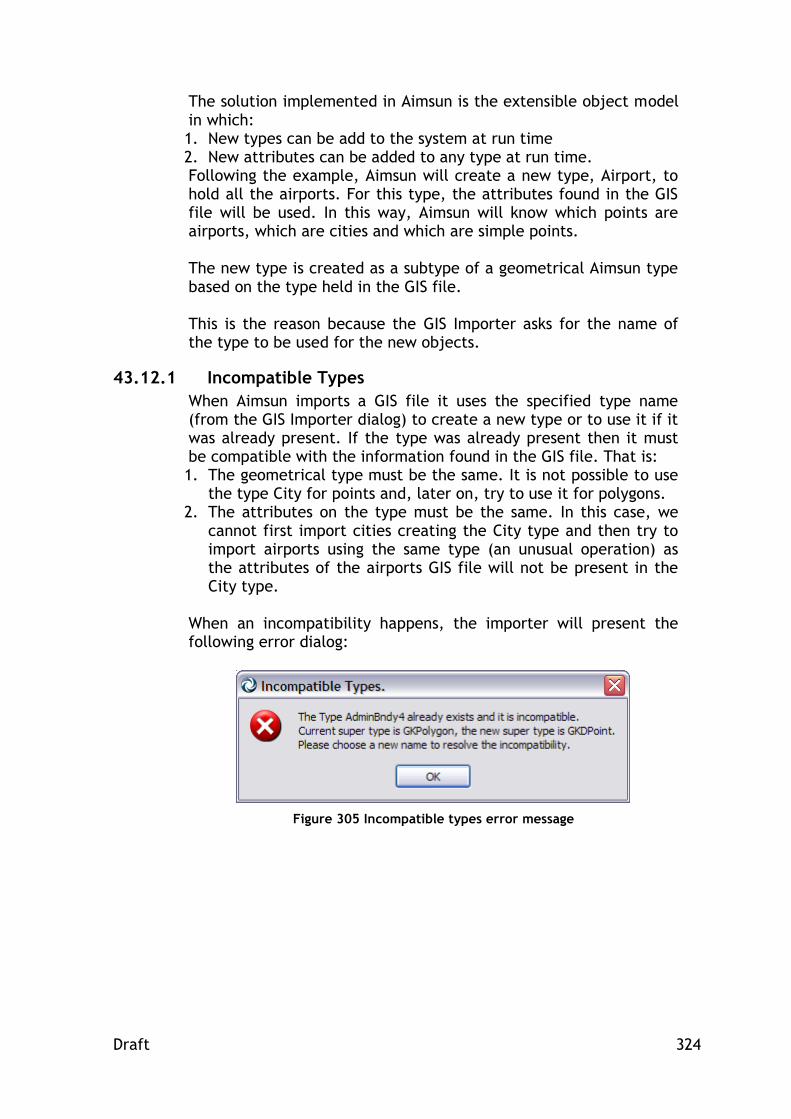
Draft 324
The solution implemented in Aimsun is the extensible object model in which: 1. New types can be add to the system at run time 2. New attributes can be added to any type at run time. Following the example, Aimsun will create a new type, Airport, to hold all the airports. For this type, the attributes found in the GIS file will be used. In this way, Aimsun will know which points are airports, which are cities and which are simple points. The new type is created as a subtype of a geometrical Aimsun type based on the type held in the GIS file. This is the reason because the GIS Importer asks for the name of the type to be used for the new objects.
43.12.1 Incompatible Types
When Aimsun imports a GIS file it uses the specified type name (from the GIS Importer dialog) to create a new type or to use it if it was already present. If the type was already present then it must be compatible with the information found in the GIS file. That is: 1. The geometrical type must be the same. It is not possible to use
the type City for points and, later on, try to use it for polygons. 2. The attributes on the type must be the same. In this case, we
cannot first import cities creating the City type and then try to import airports using the same type (an unusual operation) as the attributes of the airports GIS file will not be present in the City type.
When an incompatibility happens, the importer will present the following error dialog:
Figure 305 Incompatible types error message

Draft 325
44 OpenStreetMap Importer
You can start a new project importing a map from OpenStreetMap or you can import an OpenStreetMap onto an existing project.
44.1 Import from template
To create a new project importing an OpenStreetMap file, go to the New Project tab and zoom in at the place of interest.
Figure 306 Open Street Map New Project options
Select the desired template. By default when Aimsun is installed 4 templates customized for OSM are provided distinguishing by language. The UTM zone of the area to be imported will be set automatically. Before creating the new network, pressing the Create button, choose one of these options:

Draft 326
Do nothing: no import, just load the template as it is.
Set Area: no import, load the template and zoom to the area
(and set the UTM zone) corresponding to the map.
Import Area from the Internet: import the visible map from OSM
servers, zoom to it and set the UTM zone. Note that OSM servers
will not allow you to import large areas.
Import Area from File: import the visible map from an OSM file
in your computer. It will filter the data outside the visible map.
Will also zoom to the area and set the UTM zone.
Figure 307 Open Street Map Importation options
The last option requires that you download an OSM file from, probably, OSM Planet (http://wiki.openstreetmap.org/wiki/Planet.osm). There you will find maps by country and, sometimes, by region. When using this option, Aimsun will filter objects outside the visible map. You can for example use the map of Germany to import an area in Berlin. Note that loading and filtering large OSM files will require a lot of CPU and RAM. The OSM Importer dialog box will then come up as shown below:
Figure 308 Open Street Map New Importation options

Draft 327
The map can be used to create a draft Aimsun network (Import Road as a Network) or to import extra objects for decoration purposes (Import Decoration). It is also possible to use to map to decorate an existing network (importing parks, buildings, lakes…) without adding any traffic network element. Use, in this case the option “Import Roads: No”.
Figure 309 Open Street Map imported network
OSM can hold information on several aspects of how objects are in reality regarding its shape, size, etc. as well as regarding land use of certain areas, besides network information.
44.2 Import from menu
To add information from an OpenStreetMap to an existing Aimsun project, select the File -> Import -> OpenStreetMap files option. A file browser will appear where to select the osm file. After selecting the file to import, the dialog with the importing options described in the previous section will appear. Please refer to section 44.1 for more details. If you are importing an OpenStreetMap file to a project that was not originally created with aOSM template and you are interested in importing sections with their OSM road type please edit first the External ID of the road types that you want the new sections to

Draft 328
belong to. The Road Type’s external ID that will be used should contain the following words:
motorway
trunk
primary
secondary
tertiary
residential
pedestrian
rail
tram
subway
unclassified
For all sections with a road type defined that is not present in the Aimsun project the default road type will be assigned.
44.3 OSM 3D importation [Fast track: November 2013]
In the 3D section of the OSM Importer dialog, several options can be set up so Aimsun takes advantage of this additional information, if provided by OSM, and builds a more detailed scene for 3D rendering. The user can set up the following options:
Create Blocks for all Buildings. Aimsun creates buildings with
the height that OSM provides it with. When no height data is
provided, a flat polygon will be created instead. With this
option enabled, the user can set up a rage of heights
buildings with no height information should be created with.
This gives a much realistic look of urban areas in the 3D View
in Aimsun.
Texturize Polygons According to Land Use. With this option
enabled, Aimsun will add textures to polygons created for
known Land Uses such as parks and forest.
Create Trees. With this option enabled, Aimsun will
randomly place 3D models of trees over areas marked as
“wood” or “forest” Land Use.
44.4 OSM Licensing
Please review the license terms before using OSM data at: http://wiki.openstreetmap.org/wiki/OpenStreetMap_License

Draft 329
45 TransCAD Importer
Aimsun can import TransCAD geometry and TransCAD O/D matrices.
45.1 Importing TransCAD Geometry
To import a TransCAD network in Aimsun the following steps need to be done:
Export the TransCAD geometry to shapefiles.
Using the GIS importer in Aimsun, import the shapefiles from TransCAD into an Aimsun network. Use the option to import the shapefiles as a network. Refer to the Network Creation section for details about mapping the TransCAD attributes with the Aimsun attributes.
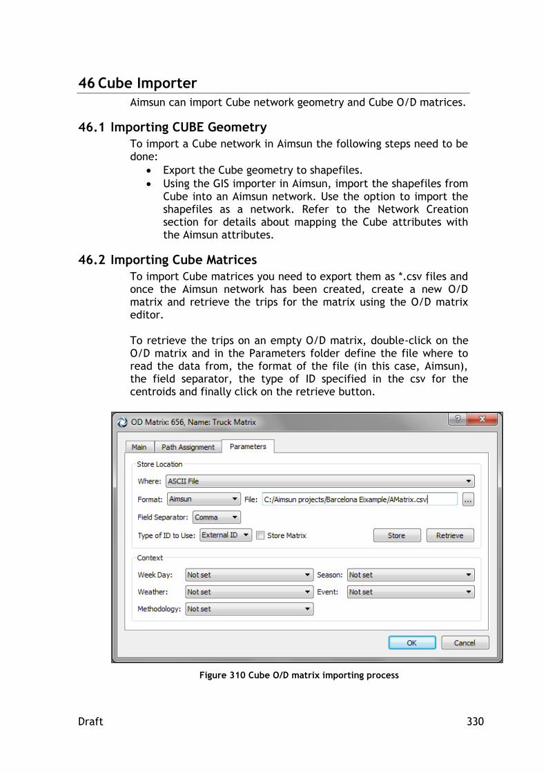
Draft 330
46 Cube Importer
Aimsun can import Cube network geometry and Cube O/D matrices.
46.1 Importing CUBE Geometry
To import a Cube network in Aimsun the following steps need to be done:
Export the Cube geometry to shapefiles.
Using the GIS importer in Aimsun, import the shapefiles from Cube into an Aimsun network. Use the option to import the shapefiles as a network. Refer to the Network Creation section for details about mapping the Cube attributes with the Aimsun attributes.
46.2 Importing Cube Matrices
To import Cube matrices you need to export them as *.csv files and once the Aimsun network has been created, create a new O/D matrix and retrieve the trips for the matrix using the O/D matrix editor. To retrieve the trips on an empty O/D matrix, double-click on the O/D matrix and in the Parameters folder define the file where to read the data from, the format of the file (in this case, Aimsun), the field separator, the type of ID specified in the csv for the centroids and finally click on the retrieve button.
Figure 310 Cube O/D matrix importing process

Draft 331
47 CONTRAM Importer
Two importation features from CONTRAM to Aimsun are available from the menu File -> Import -> CONTRAM Network (see Figure 311): to import a CONTRAM network and its CONTRAM simulation results.
Figure 311 Access to the Import CONTRAM Network menu
47.1 Importation from CONTRAM to Aimsun
The importation of a CONTRAM network consists in reading CONTRAM files3, where the main information is defined, and then translate it to an Aimsun model.
47.1.1 Importing a network from CONTRAM
To import a network, the first condition is to open a new network from menu File -> New. It is not allowed to import any CONTRAM network into an already existing Aimsun network. Then, select the menu File -> Import -> CONTRAM Network to get to the Import from CONTRAM dialog (see Figure 312). All geometrical data is described in the *.net file, so in the first slot, the user must select a file with this extension. If there isn’t any file selected, the other importing features are not allowed.
3 Only files with extension .net, .dem, .res and .rte are needed.

Draft 332
Figure 312 Import from CONTRAM dialog
The importer loads automatically all INCLUDED files, so i.e. there is no need to specify which demand files the user wants to import. The imported information relates to network geometry, control plans, vehicle types, O/D matrices, Public Transport, Traffic Management (Turn Closures) and O/D routes.
47.1.2 Importing CONTRAM simulation results
It is also possible to import the simulation results from the CONTRAM simulation and then compare them with Aimsun results. CONTRAM .res file contains time series data relative to sections such as aggregated flow, aggregated speed and flow by vehicle type; and also to turns such as aggregated turn flows. This information generates an Aimsun Real Data Set. All this information is stored in four different .csv files (located in $AIMSUN_HOME folder) and grouped in a real data set object. The time series data also contains information about centroid connectors. Note that Aimsun does not support Time Series on this kind of objects, so the retrieve real data set process will generate lots of warning messages about not finding objects. The .res file also contains information about the use percentage of simulation routes. CONTRAM .rte file contains all routes, so when loading both files, the importer will create all these routes and will assign the use percentage to the related O/D matrix.

Draft 333
47.2 Relation between CONTRAM and Aimsun objects
47.2.1 Translation a CONTRAM network to an Aimsun network
This interface imports two kinds of nodes: centroids and junctions. Centroids are defined from ZONE data, which is available in the CONTRAM network file. In the file, the position and the identifier are specified. Also, each junction is defined in NO/DE area, in the same CONTRAM file. Aimsun nodes are defined as a set of turns, so as turn data is read it is added in its Aimsun node.
Figure 313 Centroid connected to a node
Figure 314 Centroid connected to sections

Draft 334
CONTRAM also defines turns from sections that are used as centroid connectors. All this turns are translated as centroid connections that can be connected to sections or to nodes depending on node definition. In other words, if the node only contains turns from, or to, centroid connectors, then the Aimsun centroid is connected to all sections that start or end at this node (see example in Figure 314), else the centroid is connected to the node as Figure 313 shows.
47.2.2 Vehicle Types
The importer creates all vehicles defined in CONTRAM .net file. It sets Aimsun default parameters but the pcus, the Length, which is initialised with the Headway value, the Min Distance Veh, which is set to 0, the Max Desired Speed, which is set to 130km/h, and the Speed Acceptance, which is initialised with Speed value.
47.2.3 CONTRAM Maximum Speed
Maximum link speed parameter is obtained from SPEED_FLOW area, defined in CONTRAM network file. This area contains information about link categories; s_max parameter is the one that the CONTRAM Interface uses to initialize the Maximum Speed attribute.
47.2.4 O/D matrices
The number of O/D matrices that this interface creates depends on how many time slices are defined. The duration of each time slice is defined in CONTRAM network file and then assigned to each O/D matrix.
47.2.5 Control Plans
Control Plan definition is obtained from two areas: SIGNAL_PLAN and SIGNAL_TIMING, where every phase has its duration and cycle time for each node with traffic lights. Also, all turn movements that are included in each phase are specified.
47.2.6 Turn Closures
Depending on lanes restrictions, the importer will create Turn Closures that should be be added in the simulation scenario. Note that, it will create traffic management objects if all origin link groups have the same vehicle class constraint and all destination link groups have the same constraint. The aim is to keep the less restrictive condition.

Draft 335
48 Paramics Importer
The Paramics importer has two main features. The first one is the import of geometrical data of the network, so objects like sections, nodes or centroids are defined. The second one is the import of O/D matrices. This feature is available when importing geometrical data and also afterwards, when geometrical data has already been imported. The O/D matrix is created using the Centroid external ID’s. Both features are available after a new network is created using the template library. Figure 315 shows the menu path.
Figure 315 - Access to Paramics Importer Dialog
48.1 Importation from Paramics to Aimsun
Importing networks from Paramics consists of reading network files and then creation of all defined elements maintaining a very accurate correspondence between Paramics and Aimsun objects.
48.1.1 Importing a network from Paramics
The first step to import a network from Paramics is to set the directory in which Paramics files are stored. Once the path is
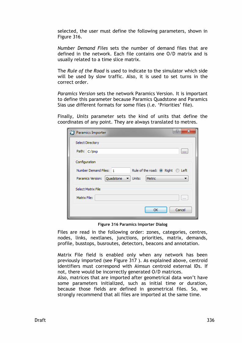
Draft 336
selected, the user must define the following parameters, shown in Figure 316. Number Demand Files sets the number of demand files that are defined in the network. Each file contains one O/D matrix and is usually related to a time slice matrix. The Rule of the Road is used to indicate to the simulator which side will be used by slow traffic. Also, it is used to set turns in the correct order. Paramics Version sets the network Paramics Version. It is important to define this parameter because Paramics Quadstone and Paramics Sias use different formats for some files (i.e. ‘Priorities’ file). Finally, Units parameter sets the kind of units that define the coordinates of any point. They are always translated to metres.
Figure 316 Paramics Importer Dialog
Files are read in the following order: zones, categories, centres, nodes, links, nextlanes, junctions, priorities, matrix, demands, profile, busstops, busroutes, detectors, beacons and annotation. Matrix File field is enabled only when any network has been previously imported (see Figure 317 ). As explained above, centroid identifiers must correspond with Aimsun centroid external IDs. If not, there would be incorrectly generated O/D matrices. Also, matrices that are imported after geometrical data won’t have some parameters initialized, such as initial time or duration, because those fields are defined in geometrical files. So, we strongly recommend that all files are imported at the same time.

Draft 337
Figure 317 Matrix Importer Dialog
48.2 Relation between Paramics and Aimsun objects
48.2.1 Nodes and centroids translation
This importer simplifies all kinds of Paramics nodes and classifies them into two categories: junction and ramp. Roundabouts are imported as junction nodes avoiding U-turns and a warning message is printed indicating the node reference, just to let the user to locate and modify it by clicking on the reference. An example of node translation is shown in Figure 318 . Only nodes with any control plan associated are marked as yellow box.
Figure 318 Node translation
Aimsun centroids and Paramics zones are strongly related. A zone is defined as an area where vehicles enter or leave the network. In Aimsun, this concept doesn’t exist, so centroids are created in the following way: 1. - The importer locates the node with the least connections that is contained in zone area.

Draft 338
2. - The position of this node will be the position of the new centroid. 3. - Centroid external ID will be set with the zone identifier. 4. - The new centroid will be connected to all sections that end or begin inside the zone area and that are floating sections; this means that one of its extreme points is not connected to any node. An example of centroid translation is shown in Figure 319 and in Figure 320.
Figure 319 Importing centroids
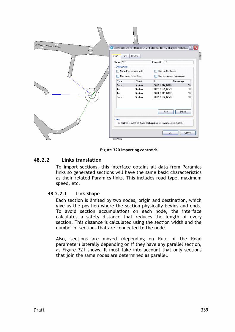
Draft 339
Figure 320 Importing centroids
48.2.2 Links translation
To import sections, this interface obtains all data from Paramics links so generated sections will have the same basic characteristics as their related Paramics links. This includes road type, maximum speed, etc.
48.2.2.1 Link Shape
Each section is limited by two nodes, origin and destination, which give us the position where the section physically begins and ends. To avoid section accumulations on each node, the interface calculates a safety distance that reduces the length of every section. This distance is calculated using the section width and the number of sections that are connected to the node. Also, sections are moved (depending on Rule of the Road parameter) laterally depending on if they have any parallel section, as Figure 321 shows. It must take into account that only sections that join the same nodes are determined as parallel.

Draft 340
Figure 321 Parallel sections
48.2.2.2 Ramps
Two situations are derived from the definition of node ramps: The first one is shown in Figure 322.
Figure 322 Ramp of Type 1
Section N4_N8 has to be connected by a ramp to the section N2_N3. This kind of ramps is easy to import since section N4_N8 ends near origin node of section N2_N3. So, this interface only has to add a new lateral lane on section N2_N3 and connect section N4_N8 to this new lane. The result of the import is shown in Figure 323.

Draft 341
Figure 323 - Connecting Ramp for Type 1
The second kind of ramp is shown in Figure 324.
Figure 324 Ramp of Type 2
In this kind of ramp, section N3479_N1823w ends in an intermediate point of section N58_N3436. The procedure to import is the following:
1. - Divide section N58_N3436 in two sections. The point where the section is cut is the projection of the N3479_N1823w end point to section N58_N3436. 2. - Connect both sections 3. - Add a lateral lane and connect N3479_N1823w to it.
Figure 325 shows the result of importing a ramp of this type. If any section has more than one ramp, this procedure is repeated for every one of them.

Draft 342
Figure 325 - Connecting Ramp for Type 2
48.2.3 Turns definition
This interface reads nextlanes and junctions files to import turns from Paramics. For each node that doesn’t appear in these files, all possible turns are created, avoiding U-turns.
Nextlanes
Nextlanes file defines specific turns from some lanes from origin section to some lanes of the i-th exit section. Figure 326 shows an example of the nextlanes import.
Figure 326 Nextlanes translation
Link 10:445 has 4 lanes at the end of the section. The white Aimsun turn is the resultant turn of the import, where all origin lanes of section N10_N445 join with the first 4 lanes of destination section (N445_N108).
Next Lanes
link 10:445
lane 1 next 1 0
lane 2 next 2 0
lane 3 next 3 0
lane 4 next 4 0
link 437:445
lane 1 next 0 5

Draft 343
The second defined turn is the red turn, which joins section N437_N445 with the 5th lane of destination section. Paramics defines two possible exits in node 445, but Aimsun only has 1, this is because Paramics also defines barred links (that are not imported). Exits are arranged in clockwise or counterclockwise direction, depending on the Rule of the Road. In this example, the vehicles drive on the right.
48.2.3.1 Junctions
The Junctions file defines, for every available exit, which are the origin lanes to which vehicles can turn (see Figure 327).
Figure 327 Junction translation
48.2.4 Priorities and Control Plans
Paramics priorities are mapped with Aimsun priorities; the next table shows the corresponding relation:
junction 401:81
out 1 lanes 1
out 2 lanes 2 3

Draft 344
Paramics Priority Aimsun Priority
Minor4 Stop
Medium Give Way
Major None
Control Plan translation is achieved as follows: For each possible turn, this interface assigns to it a signal group, so when a phase contains a turn, automatically it adds the related signal group, avoiding barred turns. Paramics importer only imports fixed control plans5, so Paramics max parameter, which initializes Minimum Green and Max-Out Aimsun parameters of an actuated control plan, is not taken into account in fixed control plans but, in actuated ones, it is used to draw the control plan in its editor.
48.2.5 Vehicles
Paramics importer creates paramics vehicles setting the Aimsun vehicle ‘car’ default values to all attributes but Length, Width, Maximum Speed, Maximum Acceleration and Maximum Deceleration, which values are adopted from Paramics Vehicles.
48.2.6 O/D matrices
All matrices are created from data obtained by processing profiles, matrix and demand files. The Profile file contains information about time slices of every related O/D matrix. Figure 328 shows an import example: In left square there is data from a profile file that specifies the time interval of the periods and the start time of every period. The percentage to apply to the matrix for the time interval is also defined. This means that, starting at 6:30 and ending at 6:45, the matrix related to period 1 represents the 100% of trips in this time.
4 Networks in Paramics SIAS don’t have Stop priority, so they will be imported as Give
Way 5 In priorities file only the max duration parameter is defined, AIMSUN actuated control
plans need more parameters (such as recall type, time to reduce, etc.) and detectors
associated to these kinds of control plans, so it is better that the user configure actuated
control plans manually.

Draft 345
Figure 328 O/D matrix import
In the case shown in Figure 329, this interface will generate 2 O/D matrices. The first one starting at 6:45 and trips will be equal to the 50% of the related Paramics matrix; the second one will start at 7:00 and will have the same trips of the first O/D matrix. Both will have 15 minutes of duration.
Figure 329 O/D matrix import
Also, the Paramics interface imports matrices defined in the ‘matrix’ file. Those matrices are not related with any time period, so they are imported as they are defined in Paramics matrix file. This interface initializes Initial Time parameter to 08:00 and 1 hour of duration. Additionaly, the vehicle type is also set to the matrix considering the vehicle’s proportion (defined in vehicles file).
Demand Profile
Profile Count 1
Profile 1
Period Count 12
Divisor 1
Interval 15
period 2 start 6:45:00
50 50
Demand Profile
Profile Count 1
Profile 1
Period Count 12
Divisor 1
Interval 15
period 1 start 6:30:00
100
...
demand period 1
matrix count 1
divisor 1.0000

Draft 346
48.2.7 Public Transport Lines
The first step to import public transport lines is to create all bus stops in the network. Then this interface creates all defined Paramics public lines and sets the time schedules for each one. The route of each public line is built taking the sections between nodes. Remember that Aimsun only allows one bus stop to be added in a section. If there is more than one bus stop on a section that is related with the same public line, it won’t be added to the public line. Figure 330 shows an example of public transport line translation.
Figure 330 Imported Public Transport Line

Draft 347
48.2.8 Detectors, Beacons (VMS) and Annotations
Detectors are placed at the distance from the beginning of the section specified in Paramics Detectors file. Next figure shows an import of a Paramics detector. Default parameters are checked on each new detector.
Figure 331 Importing a Paramics detector
Paramics beacons, as with detectors, are placed at the distance from the beginning of the related section. The user can add any text to every VMS. In order to import annotations without any problems, be sure that the text coordinates format is the following:
(xcoord_[m,ft],ycoord_[m,ft],zcoord_[m,ft])
where [m,ft] means that it is read m (metres) or ft (feet) and blank spaces are marked as ‘_’.

Draft 348
49 Vissim Importer
This importer has two main features. The first one is to import geometrical data of the network, so objects like sections, nodes or centroids are defined. The second one is to import O/D matrices. This feature is available when importing geometrical data. The O/D matrix is created using the Centroid external ID’s. The Vissim importer can import also control plan and public transport information. Both features are available after a new network is created using the template library. Figure 332 shows the menu path.
Figure 332 - Access to Vissim Importer Dialog
49.1 Importation from Vissim to Aimsun
Importing networks from Vissim consists of reading network files and then creation of all defined elements maintaining a very accurate correspondence between Vissim and Aimsun objects. This interface supports Vissim version 4.30

Draft 349
49.1.1 Importing a network from Vissim
The first step to import a network from Vissim is to set the directory in which Vissim files are stored. Once the path is selected, the geometry file *.inp and all matrices *.fma in the folder are automatically added to the editor settings, shown in Figure 333. However, it is possible to add matrices from any other folder (by clicking on Add button). Only checked matrices will be imported.
Figure 333 Vissim Importer Dialog
49.2 Relation between Vissim and Aimsun objects
49.2.1 Vissim Links and Aimsun Sections
49.2.1.1 Similarities
Vissim Links have a unique identifier, which is kept in Aimsun Sections External ID. Vissim Links can have many control points, which define the shape of the link. Aimsun Sections try to keep the original shape but simplifying the number of points Aimsun Sections will keep information like number of lanes, lane width and the length. Properties related to Road type are not imported in this version.

Draft 350
49.2.1.2 Differences
Vissim Links can have turns at any part of the link, as Vissim doesn’t define turns as Aimsun does; so, the implemented solution implies the following steps:
Split the Vissim Link in segments of length Segment Length (parameter defined in Vissim Geometry file)
Read the connectors and associate them into the segments which is at the beginning of the connector (exit turn) and the one which is at the end of the connector (input turn)
The Aimsun section will be splitted depending on the number of turns and the type of the turns at each link segment, as it is shown in the following picture
Figure 334 Section Splitting
49.2.2 Vissim Parking Lots and Aimsun Centroids
Each Vissim Parking Lot belongs to a single Zone, which are indexed by unique identifiers. In fact, the Zone plays the role of a Centroid, so when translating the network, Aimsun Centroids External ID is initialized with the Zone identifier. The Vissim Parking Lot defines the connection to or from a Vissim Link. Taking into account the FRACTION parameter, the connection can be either to a section (Fraction = 1.0) or from a section (Fraction = 0.0) The position of each Aimsun Centroid is calculated from its connections.
49.2.3 Aimsun Nodes
This is, maybe, the most difficult part of the importation. Vissim doesn’t define any kind of node, so there’s a process to join nodes once all turns have been created in Aimsun; considering the following:

Draft 351
Origin Section: All turns from a section must be at the same node
Destination Section: All turns to a section must be at the same node
Turn Intersection: A pair of intersecting turns must be at the same node
All these constraints may generate nodes either having too many turns, see Figure 335, or disjoining turns that should be in the same node, see Figure 336:
Figure 335 Node too big
Figure 336 Nodes disjoined

Draft 352
Vissim can set different stop points for vehicles while defining a control plan independently if the stop points correspond to any turn defined, so as, it may imply the creation of new turns to keep the stop points of vehicles in Vissim.
Figure 337 Node with control plan
The selected turn in Figure 337 has been created to define the control plan. Figure 338 shows that this turn belongs to the imported signal group 9.
49.2.4 Control Plans
Vissim Control Plans can be defined at any position in a section, thus, the importer will try to locate an existing node to define the control plan, if it fails, it will split the section at the specified position giving a small gap to create the a new node. Once the node has been selected, only fixed control plans will be imported.

Draft 353
Figure 338 Imported Control Plan
49.2.5 Vissim Matrices and Aimsun O/D matrices
Vissim Matrices have the trips between each pair of zones. Vissim also defines the time when the matrix is applied to the network and a scaling factor, which multiplies every single value of the matrix. Aimsun also has the same kind of definition, so the importer just sets the same values when creating new O/D matrices. The only thing it cannot initialize is the vehicle type because Vissim does not define (in the matrix file) which is the vehicle associated to the matrix.
49.2.6 Vissim Vehicle Types
From all Vissim vehicle type attributes, Aimsun can only use the length and width. So, when creating new vehicle types, car default parameters are set but length and width that are imported from Vissim.
49.2.7 Vissim Public Transport
The importer creates all public transport infrastructure (stops and lines) and then sets the timetable schedules according to Vissim definition. It also assigns the imported Vissim vehicle type if it is already defined in Vissim network file; otherwise, Aimsun "bus" vehicle type is set.

Draft 354
50 Visum Importer
50.1 Importing a network from Visum
Visum importer allows the user to import Visum networks (.net files) whose language is English, German or French. Currently supported versions range from 2.8 up to 6.0. In order to import a Visum network, go to File, Import menu and select Visum Network Files:
Figure 339 - Access to Visum Importer Dialog
50.2 Relation between Visum and Aimsun objects
Every Visum file contains a set of elements that refer to an object in the network. These objects have their counterpart in an Aimsun network:

Draft 355
Nodes and Turns: used to create Aimsun nodes and turns.
Zones: Aimsun centroids.
Connectors: Aimsun connections between objects.
Links, Link Polygons, Transport Systems and Stop Points (for public transport): A combination of these four objects result in Aimsun sections and Aimsun road types.
Lines, Line Routes and Line Route Items: they define Aimsun public transport lines and their schedules.
Detectors and Count Locations: Aimsun detectors. Also the importer looks for all the *.mtx files located in the same folder than the *.net file and creates an Aimsun matrix for each *.mtx file read. These matrices will not store the trips inside the Aimsun file but will be created as External Matrices and therefore read the trips from the corresponding *.mtx file.

Draft 356
51 Road XML Importer
Road XML is an open file format for the logical description of road networks (http://www.road-xml.org/) Road XML importer allows the user to import Road XML networks (.rnd files). In order to import a Road XML network, go to File, Import menu and select RoadXML Network:
Figure 340 Access Road XML Importer Dialog
51.1 Relation between RoadXML and Aimsun objects
Every RoadXML file contains a set of elements that refer to network objects:
Intersection: A Road XML Intersection is imported as an
Aimsun node. The link between both objects is made by
setting the Node name as the Intersection name.
All possible turns are created, except those that are banned
on each intersection.
Track: A RoadXML track is imported as an Aimsun section,
taking into account the track shape. Note that tracks can
also be reversed, so in order to link both objects, section

Draft 357
names contains the track name and also specify whether it is
reversed or not.
Tracks can have different profiles that define the width,
number of lanes, etc. Section geometry is adapted according
to the profile definition.
The information about tracks altitude is also imported.

Draft 358
52 SYNCHRO Importer and Exporter
The Synchro Importer and Exporter is aimed at using Synchro in combination with Aimsun to perform the following tasks:
optimize in Synchro the signal timings of a network modelled in Aimsun, and then quantify with a micro or meso simulation in Aimsun the results achieved
execute a Level of Service analysis in Synchro of a network modelled in Aimsun
create a draft Aimsun model from a Synchro network Starting from a calibrated Aimsun model, the workflow for the first two tasks is:
if only a portion of the whole model need to be exported, define a SubNetwork
if the turn volumes have to be read from Traffic States, create the Traffic States (either manually or with the results of a macro assignment) and group them in a Traffic Demand
if the model contains several Control Plans, create a Master Control Plan containing the Control Plan to export
launch the Synchro Exporter and select the output UTDF file to create, either the whole network or a Subnetwork, a Master Control Plan, and either a Traffic Demand based on Traffic States or a meso or micro Replication to fill the turn volumes
perform the signal optimisation and/or the Level of Service analysis in Synchro
launch the Synchro Importer to import the optimized signal timings in Aimsun
For the third task, the workflow is to create a new model in Aimsun and import the draft geometry, a Control Plan and a Traffic Demand composed by Traffic State from an existing UTDF file. The information that is interchanged includes:
geometry of the network
signal phasing and timings
turn volumes
52.1 Synchro Importer
The Synchro Importer reads a .csv file in UTDF Combined format and imports into an existing Aimsun model the signal phasing and timings, or creates a new draft Aimsun network using the geometry contained in the file, a Control Plan using signal phasing and timings and a Traffic State using the turn volumes. The Synchro Exporter is launched from the File menu, Export, Synchro Network (UTDF) option (Figure 341).

Draft 359
Figure 341 Access to the Import SYNCHRO menu
The dialog that appears allows the user to select the file to import from and whether to import everything or just the signal information.
Figure 342 Importing a Synchro Control Plan
52.2 Importing the signal information
To import only the signal information, the Import Whole Network option must not be checked.

Draft 360
The Importer will map Aimsun Nodes to Synchro Nodes using the Synchro Node ID attribute and Aimsun Turns to Synchro Lane Groups using the cardinal directions in Aimsun (Table 1). A new Control Plan containing the phasing and timings defined in the UTDF file will be created. Note that the Signal Groups are not modified, so the assignment of the Phases to the Lane Groups must be feasible with the Signal Groups defined in Aimsun6.
52.3 Importing the whole model
Create a new Aimsun Project from a template and launch the Synchro Importer. To create an Aimsun model from an UTDF file, the Import Whole Network option must be checked and the rule must be provided. The Synchro Importer builds the geometry creating a Section for each Link and a Turn and a Signal Group for each Lane Group, creates a Control Plan with the Timing Plan and Phasing information, and creates a Traffic State for light and one for heavy vehicles with the Turn Volumes. Moreover, a Master Control Plan containing the Control Plan, a Traffic Demand containing the Traffic States, a Scenario, a micro one-shot Experiment and a Replication are automatically configured.
Figure 343 Importing a Synchro network
52.4 Synchro Exporter
The Synchro Exporter creates a .csv file compliant with the UTDF (Universal Traffic Data Format) Combined format defined by Trafficware7, containing the geometry of the network, the turn volumes and the signal timings.
6 This is not an important constraint, because the correspondence between signal groups and turns in reality can be changed only changing the physical traffic lights, which is normally out of the scope of a signal optimisation study. 7 See Synchro Studio 7 User Guide, chapter 16.

Draft 361
The Synchro Exporter is launched from the File menu, Export, Synchro Network (UTDF) option (Figure 344).
Figure 344 - Access to Synchro Exporter
The dialog that appears allows the user to select the file to be created and the source of information about the geometry, the signal plans and the turn volumes (Figure 345). The path and filename of the output file is set in UTDF Combined File, under Output File. The geometry can be either taken from the whole network or from any existing Subnetwork8 that is listed in the drop-down list under Network. Aimsun allows to model different types of road infrastructures (freeways, signalized roads, etc.) in the same model, and different sizes of networks (from an isolated intersection to a whole city), while Synchro is mainly intended for isolated signalized intersections or corridors of signalized intersections. The possibility to export a Subnetwork allows reusing any existing Aimsun model, without the need to create a specific one for the study with Synchro.
8 About defining a Subnetwork in Aimsun, please refer to chapter 15 of the Aimsun User’s Manual.

Draft 362
Figure 345 Synchro exporter dialog
If the Use Geometry from an Existing UTDF File option is checked the user has the possibility to reuse an UTDF file previously exported rather than to generate it from the Aimsun model. In this case, the geometry will be taken from that file, while the signals and the turn volumes from the Aimsun model. For this option to work, the UTDF file needs to have the same node identifiers as the Aimsun network, so the best is to use a previously exported file. Provided that the network topology is not changed, in order to preserve the correspondence between the nodes and turns in Aimsun and the nodes and movements in Synchro, and that the assignment of the phases to the lane groups is feasible with the Signal Groups defined in Aimsun, this option allows conserving any subsequent editing done in Synchro, when repeating the export in order to consider a different signal plan. The signal phasing and timings are taken from the Control Plan contained into the Master Control Plan chosen among those listed under Signal Plan. Please note that only Master Control Plans containing a single Control Plan are listed: Synchro can handle only one set of phasing and timings for each intersection, therefore it is possible to export only a single control plan at a time.

Draft 363
The turn volumes can be either taken from a set of Traffic States, or from the outputs of a dynamic simulation (meso or micro). Note that it is possible to use the turn volumes of a macro assignment by creating the Traffic States from its results (Figure 346).
Figure 346 Creating Traffic States from the results of a macro assignment
If Use Traffic States is selected, a Traffic Demand containing the Traffic States to use must be chosen among those listed. To be listed, a Traffic Demand must be based on Traffic States and have one or two Vehicle Types: the Traffic State of the Vehicle Type having a PCU of 1 defines light traffic, while that of the Vehicle Type having a PCU greater than 1 defines heavy traffic. Light and heavy flows are added to calculate the total volume, and then the percentage of heavy vehicles is calculated. If Use Simulated Flows is selected, a Dynamic Scenario, a meso or micro Experiment and a Replication must be chosen from the drop-down lists. The selected replication has to be simulated with the calculation of outputs for Turns and Nodes active (Figure 347), or it has to be retrieved from the database9. The turn flow for any Vehicle Type having a PCU of 1 defines light traffic, while that for any Vehicle Type having a PCU greater than 1 defines heavy traffic10. Light and heavy flows are added to calculate the total volume, and then the percentage of heavy vehicles is calculated. Note that the start time and duration of the Master Control Plan selected under Signal Plan determines the interval of the outputs that will be exported11. Note that the turn volumes produced by a macro assignment represent the total demand, while those produced by a meso or micro simulation represent the demand served by the actual signal timings.
9 If the selected replication has not been simulated with the calculation of outputs for Turns and Nodes active, or it has not been retrieved from the database, the exported volumes will be 0. 10 Note that, unlike when using Traffic State, using simulated flows there is no limit to the number of Vehicle Types. 11 The exported flow is the average of the flows during the intervals that fall at least partially inside the schedule of the Master Control Plan, weighted with the proportion between the portion that falls inside the schedule and the total duration of the interval.

Draft 364
Figure 347 - Output calculation for Turns and Nodes
The Exporter assigns a new unique ID to all the nodes exported to Synchro (intersection, bend and external nodes)12; it adds a column to the Nodes in Aimsun, called Synchro Node ID, where the automatically generated Synchro ID for the exported nodes is stored, and adds two columns to the Sections in Aimsun, called Synchro Node Origin and Synchro Node Destination, where the Synchro IDs of the extreme nodes are. These attributes are used by the Exporter, in case Use Geometry from an Existing UTDF File is checked, and by the Importer, in case Import Whole Network is not checked, to establish a correspondence between Nodes and Sections in Aimsun and Nodes and Links in a UTDF file. Note that the Exporter assigns the cardinal directions to approaches and lane groups according to the actual angle in Aimsun (Table 1), and doesn’t apply any automatic rotation to simplify diagonal intersections with four or less legs.
Angle13 Direction
-π/8 < α ≤ π/8 EB π/8 < α ≤ 3π/8 NEB 3π/8 < α ≤ 5π/8 NB 5π/8 < α ≤ 7π/8 NWB
7π/8 < α or α ≤ -7π/8 WB -7π/8 < α ≤ -5π/8 SWB -5π/8 < α ≤ -3π/8 SB -7π/8 < α ≤ -π/8 SEB
Table 1 Approach and lane group designations
12 Synchro node numbers can range from 1 to 9999. 13 Angles in Aimsun are measured from the east direction and are positive (from 0 to π) going to north and negative (from 0 to -π) going to south.

Draft 365
Ideally, it is possible to change the values stored to match those of an existing Synchro network even if not exported from Aimsun, but it is user’s responsibility to assure that the orientation of the network and the topology are the same.
52.5 Naming conventions for signal control parameters The following table shows the relation between the names used in Aimsun and those used in the UTDF file for signal control parameters.
Aimsun UTDF
Barrier, Ring, Position BRP Minimum Green, Maximum
Initial Green MinGreen
Max-Out MaxGreen Passage Time VehExt
Time Before Reduce TimeBeforeReduce Time To Reduce TimeToReduce
Passage Time MinGap Yellow Time Yellow
Interphase Time AllRed Recall Recall
Table 2. Naming conventions for NEMA parameters
Permissive Period From, Permissive Period To and Force Off are initialized automatically.

Draft 366
53 3D File Importer and Exporter
53.1 Importer
The 3D File Importer allows the user to include 3D models into an Aimsun network. Found under File-> Import -> 3D File it can import 3D models in the following formats:
Autodesk 3ds Max (.3ds filename extension)
Wavefront OBJ (.obj filename extension)
Open Scene Graph native formats o Binary format (.ive filename extension) o Text format (.osg filename extension)
Once the 3D model is selected through the “Open File” dialog, it will be imported into the current document in Aimsun. It’s editing will be therefore available at the 2D and 3D Views.
53.2 Exporter
The 3D File Exporter allows the user to export the network’s geometry into 3rd party 3D modelling software tools, enabling the user to create rich 3D scenes around networks created with Aimsun. The geometry exported currently includes Nodes and Sections. The option is found under File-> Export -> Network as 3D File. Notice that before exporting a network in 3D format, a 3D View should be opened in Aimsun. The following formats are supported:
Autodesk 3ds Max (.3ds filename extension)
Open Scene Graph native formats o Binary format (.ive filename extension) o Text format (.osg filename extension)

Draft 367

Draft 368
54 Aimsun Licensing
This chapter covers how to deal with Aimsun licenses successfully.
54.1 Licensing technology
Aimsun can be licensed using the HASP SRM technology.
In this type of license the information is written inside the dongle. When the user receives the dongle for the first time the license is already written in the dongle. It contains the expiry date, the features and the SUS date.
To consult any license details and perform other actions the user has to go to the following address:
http://localhost:1947
Selecting the option HASP Keys all the dongles used will be shown. All the dongles belonging to TSS will have the vendor number 78046.
Selecting the option Products a list of the available products is shown as below:
Similarly the option Features can show relevant details as shown below:

Draft 369
These details include the features contracted, the number of users and the expiration date of the license.
If no products or features are listed this might indicate the Aimsun license for that dongle is based on Flexlm instead of HASP SRM. Please contact [email protected] in case of doubt.
54.1.1 Updating a HASP SRM license
In order to update dongles based on this type of license the user has to receive a v2c file from TSS and apply it to the dongle just once. To update a HASP SRM type dongle there are two options:
1. Run [Aimsun Folder]\licenses\utils\rus_Aimsun.exe and
select the Apply License Update tab. Then load the v2c file received from TSS.
2. From the page http://localhost:1947 select the option Update/Attach and load the v2c file received from TSS.
54.1.2 Checking the state of a HASP SRM license
To verify the state of a HASP SRM license, TSS might ask the user to generate and send to TSS a c2v file with the dongle details.
In order to create the c2v file, the user must go to [Aimsun Folder]\licenses\utils\rus_Aimsun.exe and run it. Under the tab Collect Key Status Information the c2v file can be generated by pressing the Collect Information button.
54.1.3 HASP SRM Network licenses
To configure HASP SRM network licenses refer to the Aimsun HASP SRM Network License Installation Guide.
For this type of network licences the user has to set the following options in the server and the client computer as shown below:

Draft 370
Server configuration
Client configuration
54.2 Licensing options
54.2.1 Multiple dongle options
In case the user has more than one Aimsun dongle, in Aimsun 7 there is a new option for the user to force Aimsun to work with a certain dongle. Using either the command prompt or editing the Aimsun shortcut the user can write:
[Aimsun Directory]\aimsun.exe –dongleid XXX (where XXX is
the dongle ID that you want Aimsun to work with)
54.3 Legion for Aimsun licensing
A Legion for Aimsun license is required to use the embedded Legion pedestrian simulator in Aimsun. It is available for the 32bits and 64 versions for Windows. In order to get it:
Open the Help/Licenses... menu from Aimsun
Click on Request License button and the following dialog
brings up:

Draft 371
Click on Email Request button to send an automatically
generated form file to [email protected] or click on Save
To File button to generate the form. Remember to send the
form to TSS ([email protected]).
Once TSS sends you back the Legion for Aimsun license, open
the Help/Licenses... menu from Aimsun.
Click on Install License button and the following dialog brings
up:
You can have a look at the licence as well as at the schedule
that will give you the details about your Legion for Aimsun
licence.
Select I Agree to install your licence and then click on the
Close button.
54.4 License troubleshooting
If after following the steps to correctly install a license, Aimsun does not execute please try the following:
Verify that the dongle is connected and the light (when
applicable) is on)
Go to http://localhost:1947 and verify that all the data is
correct (expiry date and features) according to what was
contracted with TSS.
The SUS is not visible to the user, therefore it can be
consulted by asking TSS. In the case that Aimsun is executing
the information is in Help -> Licenses.

Draft 372
If after installing the license, Aimsun does execute but the user cannot simulate the replications it is definitely not a license problem:
Go to Help -> About Plugins
If there are modules marked with a red icon, please re-
install Aimsun after making sure that the previous install
directory is totally deleted.
If after installing the license, Aimsun’s Legion for Aimsun cannot simulate pedestrians:
In the Aimsun directory check if there are following Legion
library files (.dll). If not re-install Legion for Aimsun.
In Help -> Licenses, make sure the Legion license is loaded
correctly such as below. If not load the .lic file.
If after those checks the license is still not activating Aimsun please contact [email protected] .


