DEVELOPMENT OF AVAILABILITY AND SUSTAINABILITY SPARES OPTIMIZATION MODELS FOR AIRCRAFT REPARABLES THESIS Edmund K.W. Pek, Major (Military Expert 5), RSAF (Republic of Singapore Air Force) AFIT-ENS-13-S-4 DEPARTMENT OF THE AIR FORCE AIR UNIVERSITY AIR FORCE INSTITUTE OF TECHNOLOGY Wright-Patterson Air Force Base, Ohio DISTRIBUTION STATEMENT A: APPROVED FOR PUBLIC RELEASE; DISTRIBUTION UNLIMITED.
Transcript
DEVELOPMENT OF AVAILABILITY AND SUSTAINABILITY
SPARES OPTIMIZATION MODELS FOR AIRCRAFT REPARABLES
THESIS
Edmund K.W. Pek, Major (Military Expert 5), RSAF (Republic of Singapore Air Force)
AFIT-ENS-13-S-4
DEPARTMENT OF THE AIR FORCE AIR UNIVERSITY
AIR FORCE INSTITUTE OF TECHNOLOGY
Wright-Patterson Air Force Base, Ohio
DISTRIBUTION STATEMENT A: APPROVED FOR PUBLIC RELEASE; DISTRIBUTION UNLIMITED.
The views expressed in this thesis are those of the author and do not reflect the official policy or position of the United States Air Force, Department of Defense, or the United States Government nor do it reflect the official policy or position of the Republic of Singapore Air Force, Ministry of Defence, or the Singapore Government.
AFIT-ENS-13-S-4
DEVELOPMENT OF AVAILABILITY AND SUSTAINABILITY SPARES OPTIMIZATION MODELS FOR AIRCRAFT REPARABLES
THESIS
Presented to the Faculty
Department of Operational Sciences
Graduate School of Engineering and Management
Air Force Institute of Technology
Air University
Air Education and Training Command
In Partial Fulfillment of the Requirements for the
Degree of Master of Science in Logistics and Supply Chain Management
Edmund K.W. Pek
Major (Military Expert 5), RSAF
September 2013
DISTRIBUTION STATEMENT A: APPROVED FOR PUBLIC RELEASE; DISTRIBUTION UNLIMITED.
AFIT-ENS-13-S-4
DEVELOPMENT OF AVAILABILITY AND SUSTAINABILITY SPARES OPTIMIZATION MODELS FOR AIRCRAFT REPARABLES
Edmund K.W. Pek, Major (Military Expert 5), RSAF
Approved:
//signed// 05 September 2013 Dr. Alan W. Johnson (Chair) Date
//signed// 05 September 2013 LtCol. Joseph R. Huscroft, Ph.D. (Member) Date
iv
AFIT-ENS-13-S-4
Abstract
The Republic of Singapore Air Force (RSAF) conducts Logistics Support
Analysis (LSA) studies in various engineering and logistics efforts on the myriad of air
defense weapon systems. In these studies, inventory spares provisioning, availability and
sustainability analyses are key focus areas to ensure asset sustenance. In particular,
OPUS10, a commercial-off-the-shelf software, is extensively used to conduct reparable
spares optimization in acquisition programs. However, it is limited in its ability to
conduct availability and sustainability analyses of time-varying operational demands,
which are crucial in Operations & Support (O&S) and contingency planning. As the
RSAF seeks expansion in its force structure to include more sophisticated weapon
systems, the operating environment will become more complex. Agile and responsive
logistics solutions are needed to ensure the RSAF engineering community stays abreast
and consistently push for deepening competencies, particularly in LSA capabilities.
This research is aimed at the development of a model solution that combines
spares optimization and sustainability capabilities to meet the dynamic requirements in
O&S and contingency operations planning. In particular, a unique dynamic operational
profile conversion model was developed to realize these capabilities in the combined
solution. It is envisaged that the research effort would afford the ease of use, versatility,
speed and accuracy required in LSA studies, in order to provide the necessary edge in
inventory reparable spares modeling.
v
Dedication
This thesis is dedicated to my Wife and soon to be born Son for their patience and understanding throughout my time at the Air Force Institute of Technology.
vi
Acknowledgments
My most sincere thanks go to my family for their patience and understanding
throughout my AFIT experience, but especially for the many endless hours I spent
developing this research. Also, I would like to express my gratitude to Dr. Alan Johnson
for his valuable guidance, complete trust and autonomy shown to me, without whom I
could not have imagined putting this research together in a short span of time. Likewise,
I would like to acknowledge my thesis reader, LtCol. (Dr.) Joseph Huscroft, for his
frequent and pertinent advice throughout my research and coursework in AFIT. In
addition, I wish to acknowledge the friendship and hard work of my fellow logistics
management students, who have made my journey this one year all the more meaningful.
Finally, I would like to thank my colleagues in both Air Engineering and Logistics
Department and Defence Science & Technology Agency who provided the valuable
support which I so crucially required in the course of this research.
vii
Table of Contents
Abstract .............................................................................................................................. iv Dedication ........................................................................................................................... v Acknowledgments.............................................................................................................. vi List of Figures .................................................................................................................... ix List of Tables ...................................................................................................................... x List of Equations ................................................................................................................ xi List of Acronyms ............................................................................................................. xiii I. Introduction .................................................................................................................. 1
Overview ................................................................................................................. 1 Problem Background .............................................................................................. 2 Research Objectives ................................................................................................ 3 Research Motivation ............................................................................................... 4
II. Literature Review ........................................................................................................ 6
RSAF Reparable Repair Cycle ............................................................................... 6 OPUS10 .................................................................................................................. 8 METRIC Models .................................................................................................. 11 Perspectives of the Current Research ................................................................... 13
III. Methodology ............................................................................................................ 17
Conceptual Flow ................................................................................................... 17 Assumptions .......................................................................................................... 19 Data Collection ..................................................................................................... 21 Fundamental Inventory Modeling Equations........................................................ 22
Utilization Rate Effects .............................................................................. 34 UR vs Ao................................................................................................ 34 UR vs LI/LD TAT ................................................................................. 35 UR vs OD TAT ...................................................................................... 36
Sustainability Analysis Treatment .................................................................... 37 Non-Linear Programming (NLP) Model Development ........................................ 38
IV. Results and Analysis ................................................................................................ 40
Verification and Validation................................................................................... 40 Model Setup ...................................................................................................... 40 NLP and OPUS10 Models Comparison ........................................................... 42 NLP Binomial/ Negative Binomial and Poisson Models Comparison ............. 43
Sustainability Analysis.......................................................................................... 45 Model Run-Time Performance ............................................................................. 48
V. Conclusion and Recommendation ............................................................................ 50
Conclusion of Research ........................................................................................ 50 Significance of Research....................................................................................... 51 Recommendations for Action ............................................................................... 51 Recommendations for Future Research ................................................................ 52
Appendix A. Spares Data ................................................................................................. 54 Appendix B. Combined Spares Data and Logistics Parameters ...................................... 55 Appendix C. Dynamic Operational Profile Conversion Model ....................................... 56 Appendix D. Item Backorders and System Performance Computations ......................... 59 Appendix E. Excel VBA® Macro Programming Scripts ................................................ 61 Appendix F. Non-Linear Programming Logic................................................................. 65 Appendix G. NLP Poisson Model vs OPUS Model Data Output ................................... 66 Appendix H. OPUS Model Cost-Effectiveness Output ................................................... 67 Bibliography ..................................................................................................................... 68 Vita .................................................................................................................................... 70
ix
List of Figures
Page
Figure 2-1. RSAF Reparable Maintenance Support Scenario ........................................... 6 Figure 2-2. OPUS10 Sample Cost-Effectiveness (Availability vs Cost) Curve ................ 9 Figure 2-3. VARI-METRIC Pipeline Visualization ........................................................ 14 Figure 3-1. Research Conceptual Flow Chart .................................................................. 18 Figure 3-2. RSAF Reparable Calculation Sequence ........................................................ 30 Figure 4-1. NLP Model vs OPUS Model Poisson Output ............................................... 42 Figure 4-2. NLP Model Bin/NegBin vs Poisson Outputs ................................................ 44 Figure 4-3. NLP Model Output for Spares Package Selection ........................................ 45 Figure 4-4. Sustainability Analyses of Spares Packages ................................................. 46
x
List of Tables
Page
Table 2-1. Time Required in OPUS10 LSA Studies ....................................................... 10 Table 4-1. Comparison of Time Required for OPUS10 and NLP Model Studies ........... 49
Equation 22. Weighted LI/LD Item TAT Equation ......................................................... 36 Equation 23. Average Utilization Rate Equation ............................................................. 37 Equation 24. Weighted OD Item TAT Equation (for Optimization) ............................... 37 Equation 25. Weighted OD Item TAT Equation (for Sustainability Analysis) ............... 38
xiii
List of Acronyms
AAM: Aircraft Availability Model AELO: Air Engineering and Logistics Organization Ao: Operational Availability ASM: Aircraft Sustainability Model Bin: Binomial CE: Cost-Effectiveness D: Depot DSTA: Defence Science & Technology Agency DYNA-METRIC: Dynamic Multi-Echelon Technique for Recoverable Item Control EBO: Expected Backorder EOQ: Economic Order Quantity ERP: Enterprise Resource Planning FH: Flying Hours FMS: Foreign Military Sales GRG: Generalized Reduced Gradient HQ: Headquarters I: Intermediate ILS: Integrated Logistics Support LCM: Life Cycle Management LD: Local Depot LI: Local Intermediate LRU: Line Replaceable Unit LSA: Logistics Support Analysis METRIC: Multi-Echelon Technique for Recoverable Item Control MOD-METRIC: Modified Multi-Echelon Technique for Recoverable Item Control MSD: Mean Supply Delay MTBF: Mean Time Between Failure MTTR: Mean Time To Repair Neg Bin: Negative Binomial NLP: Non-Linear Programming O: Operational O&S: Operations & Support OD: Overseas Depot OEM: Original Equipment Manufacturers OID: Operational, Intermediate and Depot OPUS10: Optimization of Units as Spares OST: Order & Ship Time PLT: Procurement Lead Time PM: Preventive Maintenance QPNHA: Quantity Per Next Higher Assembly RAMS: Reliability, Availability, Maintainability & Supportability RLT: Repair Lead Time RSAF: Republic of Singapore Air Force
xiv
SRU: Shop Replaceable Unit SSRU: Sub-Shop Replaceable Unit TAT: Turnaround Time TPTA: Third-Party Technology Transfer Agreements UR: Utilization Rate USAF: United States Air Force V&V: Verification and Validation VARI-METRIC: Variance Multi-Echelon Technique for Recoverable Item Control VBO: Variance Backorder VTMR: Variance To Mean Ratio WF: Weighting Factor WUC: Work Unit Code WYSIWYG: What You See Is What You Get
1
I. Introduction
Overview
This paper discusses Republic of Singapore Air Force inventory modeling of
reparable spares. The Republic of Singapore Air Force (RSAF) conducts Logistics
Support Analysis (LSA) studies in support of the various engineering and logistics efforts
on the myriad of air defense weapon systems. Depending on the Life Cycle Management
(LCM) phases of the weapon system, these studies can take the form of Reliability,
Availability, Maintainability & Supportability (RAMS) front-end system definition
analyses; and Maintenance Support Planning & Capability Generation analyses for
Integrated Logistics Support (ILS) during Acquisition and Operations & Support (O&S)
phases. In particular, spares provisioning, availability and sustainability are focus areas
in LSA studies to optimize the support for weapon systems, spanning all phases of the
LCM. This is especially crucial in an Air Force that operates with a relatively small force
structure and heavily reliant on both Foreign Military Sales (FMS) and Original
Equipment Manufacturers (OEM) for the continuous supply of aircraft spares to sustain
fast changing operational requirements. In addition, the deterrence and diplomacy nature
of the RSAF mission means that operational requirements manifest as planning
parameters rather than real operations, and hence, grounded forecasting mechanisms play
vital roles in resource optimization.
Because of the realities that the RSAF faces in the conduct of her missions, a
comprehensive suite of commercial off-the-shelf software had been acquired over the
years for performing the various LSA studies. Specifically, reparable spares inventory
modeling is conducted through the Optimization of Units as Spares (OPUS10) software
2
(DISO, 2009:10-1 to 10-2). OPUS10 is a computer-based analytical software developed
by Systecon®, a Swedish company with customers that include Defense Authorities in
USA, Great Britain and Australia. It is an optimization software that uses a mathematical
analytic model to analyze critical factors affecting a weapon system’s availability and its
associated spares build-up costs. The RSAF had been employing OPUS10 in many
weapon system acquisition studies to primarily determine the optimum spares support
package, given expected operating parameters and logistics & maintenance design plans
on new induction platforms. Due to its extensive use in the RSAF, OPUS10 is also being
employed during O&S phases to conduct regular reparable spares review and “top-up”
purchases, complementing consumable spares Economic Order Quantity (EOQ) studies
automated through the integrated SAP® Enterprise Resource Planning (ERP) information
system of the RSAF. A more in-depth review of OPUS10 capabilities will be provided in
the Literature Review chapter.
Problem Background
Although OPUS10 provides a compatible tool in acquisition settings where
advance planning can be undertaken with detailed construction of the spares hierarchical
structure, its performance is rather stretched in analyzing O&S phases of spares
sustainment which warrants time-sensitive assessment of spares bottlenecks and the
consequent effects on weapon system availability assessment. In particular, it is not well
suited for analyzing multi-indenture and multi-echelon interactions of aircraft reparables
and sensitivity analyses, which are evident in RSAF’s O&S logistics structures,
organized around Operational, Intermediate and Depot (OID) level maintenance systems.
Moreover, the heavy reliance on OPUS10 over the years, results in curtailing of
3
fundamental competencies in spares reserve planning. Users become inapt to provide
additional insights on effects of surge planning and supply chain constraints as a result of
the limitations of the OPUS10 software. The author of this research had first-hand
experience with operating OPUS10 and constantly faced the challenge to provide
accurate and quick assessment of weapon system availability to decision makers in
Exercise planning scenarios.
It became apparent that a novel solution that affords ease of use, versatility, speed
and accuracy must be developed for studying spares optimization and sustainability in
O&S planning and contingency operations. This forms the basis of the research problem.
Research Objectives
The intent of this research is to develop a model solution that affords ease of use,
versatility, speed and accuracy in spares optimization and sustainability analyses
conducted for O&S planning and contingency operations.
From the above main problem statement, three investigative questions were
examined in this research:
(1) What model solution can be developed to combine ease of use, versatility, speed
and accuracy for spares analyses?
(2) What model solution can be developed to conduct spares optimization and
sustainability analyses for O&S planning and contingency operations?
(3) How can the developed model solution be validated for practical deployment?
4
Research Motivation
This research is timely as the RSAF seeks expansion in its force structure to
include more sophisticated weapon systems, such as the F-35 Joint Strike Fighter. The
Engineering and Logistics arm of the RSAF, the Air Engineering and Logistics
Organization (AELO), must constantly seek agile and responsive logistics solutions in
ensuring she meets the engineering demand of the Third Generation RSAF
transformation (Ng, 2012:36). In addition, the roll out of the Military Domain Experts
Scheme (MINDEF, 2009:7) in the RSAF engineering community also meant a push for
deepening competencies in all logistics career fields and it is opportune to fundamentally
reshape expertise in functional areas like the RSAF Supply Chain Management. It is thus
envisioned that the conduct of this research will not only ground supply chain material
planners in their core competencies but also ensure that they are able to conduct swift,
accurate and credible inventory spares analyses to support O&S and Exercise planning
and hence expand expertise on operational spares planning on future operating concepts.
This paper explores the development of a model solution that affords ease of use,
versatility, speed and accuracy in spares optimization and sustainability analyses
conducted for O&S planning and contingency operations. First, a literature review
provides an overview of the RSAF reparable repair cycle, outlining the limitations of
OPUS10 in the conduct of LSA studies. The review will also cover fundamental
inventory METRIC models in use in other military establishments to build the foundation
for development of the unique model solution. A description of the solution
methodology will then be discussed, followed by an analysis of the results of model
5
development, verification and validation. Finally, recommendations for implementation
of the model and avenues for further research will be presented.
6
II. Literature Review
RSAF Reparable Repair Cycle
Operational, Intermediate and Depot (OID) Levels Maintenance Support
Concepts are documented in Air Force Logistics Orders (AELO, 2012:1-4) and the
Singapore Ministry of Defence Life Cycle Management Manual (DISO 2009:5-1 to 5-5).
Such concepts describe the inter-relationships of repair processes of RSAF’s organic
operational (O) level Line Replaceable Units (LRUs) and intermediate (I) level Shop
Replaceable Units (SRUs), and strategic contractor’s depot (D) Level Sub-Shop
Replaceable Units (SSRUs). Figure 2-1 depicts a typical maintenance support scenario:
Figure 2-1. RSAF Reparable Maintenance Support Scenario
On-Site Workshop (I Level Repair)
Off-Site Local Depot (LD Level Repair)
Site Store (Spares Warehouse)
Operating Site (O Level Maintenance)
Failed LRUs Operational
LRUs
MTTR
Failed LRUs with I Level Repair Cap
Failed SRUs with Local D Level Repair Cap
Operational LRUs
Operational SRUs
Failed LRUs with Overseas OEM Repair Cap
Failed SRUs with Overseas OEM Repair Cap
Off-Site Overseas
OEM Depot (OD Level
Repair
TWS TSW
TLDW TWLD
TOD
TOD
RLTI
RLTLD
RLTOD
7
With reference to Figure 2-1, each operating site (air base) has several weapon
systems (aircraft), the use of which generates LRU failures and thus demands for
replacement components. Each site has its own aircraft repair crew that removes and
replaces failed LRUs based on an average Mean Time To Repair (MTTR), inclusive of
the time it takes for drawing serviceable spares from the site store. A spare LRU is
issued if one is on hand, else a backorder is established.
A failed LRU enters the pipeline network when it is sent from the store to either
the on-site workshop for I level repairs or to the OEM for Overseas Depot (OD) repair,
based on the maintenance capability designated for the LRU. For LRU with I level repair
capability only, the associated turnaround time (pipeline time) comprises both shipment
times from store to on-site workshop (Tsw) and from on-site workshop back to store
(Tws), plus the repair lead time (RLT) of the I level workshop (RLTI). While for LRU
with OD repair capability only, the turnaround time comprises the shipment time to and
from the OEM (TOD) and the agreed contractual RLT (RLTOD).
During the process when a failed LRU is repaired in the on-site workshop, a
second-indenture, SRU is identified as having failed. If a spare SRU is available in the
workshop, the failed SRU is removed and replaced by the workshop repair crew and the
LRU repair is completed, otherwise an SRU backorder is established at either the
strategic contractor Local Depot (LD) or the OEM for OD repair, depending again on the
maintenance capability designated for the SRU.
The weapon systems supported by the store constantly generates demands that
consume spares in the store. The average pipeline time translates to average pipeline size
(average lead time demand) through the individual component failure rate (that is,
8
demand rate). This pipeline size describes the total number of LRUs or SRUs that have
left either the on-site store or workshop for repair but have not returned from the
respective repair agency. AELO uses this concept in its spares acquisition programs to
define peacetime requirements for weapon system induction (DISO, 2009:10-1).
OPUS10
OPUS10 (Optimisation of Units as Spares) is a steady-state Logistics Support
Analysis (LSA) software designed to calculate optimized cost-availability of spares and
their distribution in the maintenance support organization (Systecon AB, 2007:1-4). An
operational scenario with aircraft deployment, utilisation profiles and logistics stations
(stores, workshops and depots) is modeled to establish a joint pattern of demand for
logistics support. Maintenance and logistics activities (e.g. failure rate, inventory support
concept) are also modeled. With this information, the software outputs optimal spares
packages to support different required operational availability (Ao). This optimal spare
package is a result of the “best-possible” relationship between cost and operational
availability.
Central to the OPUS10 model is an analytic stationary Poisson process model.
The computations are based on evaluating the pipeline sizes of the components given the
maintenance structure, operational demands and average failure rates. These pipeline
sizes translate to expected backorders and an optimization is performed to trade-off
between Ao and cost of spares to produce a Cost-Effectiveness Curve as shown in Figure
2-2:
9
Figure 2-2. OPUS10 Sample Cost-Effectiveness (Availability vs Cost) Curve
OPUS10 modeling concept is purely analytical and requires stationary operational
demand parameters. While this ensures LSA studies can be easily and quickly computed,
it is rather limited in its ability to model highly varied operational demand patterns (for
example, frequently changing flying profiles in contingency operations). In addition, the
highly customized graphic user interface also meant that the optimization engine behind
OPUS10 modeling is completely hidden from the user. While this takes away the
mathematical woes of the analyst, it results in curtailing of competencies in
understanding the fundamentals behind the model, which is key when conducting
sensitivity analyses of changes of logistics variables often encountered in O&S and
contingency operations. In addition, the speed afforded by OPUS10 is only as good as
the run time and much attention is instead spent in constructing the model inputs. The
author of this research collated data for a prior study in 2009 and determined a 90
minutes average requirement for conducting an OPUS10 LSA analysis:
10
Category Sequential tasks for a single analysis Time Required
(mins)
Data Entry
Collate and manipulate input data in Excel 15
Convert input data to software input format 30
Modeling
Create / Modify existing software's operations and logistics profile model 25
Input of data into OPUS10 software 10
Results Output
Generate run results 5
Analyze results 5
Total Time Required 90 mins
Table 2-1. Time Required in OPUS10 LSA Studies
Another limitation of OPUS10 is its (s-1, s) inventory model for reparables.
Although this is well suited for modeling low demand, high cost LRUs and SRUs, it may
not accurately represent the high demand and low cost SSRUs. This is apparent in AELO
case where current inventory policies do not spell out the modelling techniques for such
items. OPUS10 was never designed for modelling these lower indenture items and an
Economic Order Quantity (EOQ) model may perform better to implement a reorder
point, order quantity (R, Q) policy for SSRUs. Finally, the Poisson process assumption
used by OPUS10 postulates all components fail at random, with a Variance-to-Mean-
Ratio (VTMR) of 1. This may not accurately represent in-service reparables which
commonly fail due to wear-out (VTMR < 1) or due to reliability deterioration (VTMR >
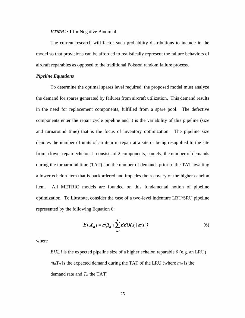
1) (Adams et al., 1994:7 and 26-27; Sherbrooke, 2004: 62-63, 89-91).
Notwithstanding the limitations, this research will build upon the strength of the
analytical methodology of OPUS10 to harness its concept of ease of use and speed, while
11
negating the limitations by revisiting the fundamentals in reparables inventory modeling
and modifying the baseline concept for more accurate and versatile model development.
METRIC Models
The mathematical concepts behind OPUS10 can be traced to the Multi-Echelon
Technique for Recoverable Item Control (METRIC) (Sherbrooke, 1968: 122-141).
METRIC is a base-depot supply system model that calculates the optimal (s-1, s)
stockage level for LRU items at each of several bases and the supporting depot. It
utilizes the concept of minimization of the base backorders in relation to the demand
patterns in both the base and the depot. This results in a systems level approach to
stocking spares by analyzing the relation between backorders and system availability. A
systems cost effectiveness curve is obtained by analysing the marginal benefit of
increased availability from the next best option in spares purchase in terms of reduced
overall system backorders (“bang per buck”). The METRIC model was a natural
transition from Sherbrooke’s prior work on the single indenture, single echelon Base
Stockage Model (Feeney et al., 1965: 391-411).
Central to the METRIC model is the infinite channel queueing assumption of the
Palm’s Theorem (Sherbrooke, 2004: 22), which assumes demand for an item follows a
Poisson process and that the probability distribution of the pipeline size is also Poisson.
While this simplifies computations, item failure rates are consequently assumed to follow
a VTMR of 1. However, this poorly models reliability deterioration and wear-out
phenomena associated with aircraft components. This resulted in less than optimal
prediction performance of the METRIC model, underestimating the items backorders
leading to higher than observed operational availabilities and lower spare stockage levels.
12
The MOD-METRIC model (Muckstadt, 1973: 472-481) extended the multi-
echelon base-depot supply to encompass analysis of multi-indenture systems (LRUs and
SRUs) while retaining the stationary Poisson assumption. The complex dependencies
from both the echelon and indenture structures further understate the backorders by
nearly a factor of 4 (Sherbrooke, 2004: 67). Subsequent works from Gross, Graves and
1256; Sherbrooke, 1986: 311-319) perfected the inventory modeling technique with the
introduction of the VARI-METRIC model to generalize the stationary Poisson process to
better model failure distributions described by the Binomial probabilities (for VTMR < 1)
and Negative Binomial (for VTMR > 1).
The VARI-METRIC model afforded better accuracy with stock level deviation of
1 unit observed only in less than 1% of the case studies analyzed (Sherbrooke, 2004:
102). It was eventually adopted by USAF in the form of the Aircraft Availability Model
(AAM) and is used for computing peacetime spares requirement (O’Malley, 1983: 1-3;
Sherbrooke, 2004: 228; Blazer, 2007: 67-68). It became the benchmark inventory
modeling technique, even till today, due to its robust modeling fundamentals and well
documented mathematical solutions. However, it was strictly confined to peacetime
spares modeling due to its requirement of a homogeneous Poisson process (that is,
constant failure/demand rate). The concepts of VARI-METRIC were later modified into
the Dyna-METRIC model to allow the conduct of wartime sustainability studies, which
are characterized by varying periods of operational demands. Dyna-METRIC utilizes a
dynamic form of Palm’s theorem to effectively change the items’ failure/demand rates
based on planned changes to the flying profile. However, it is best described as an
13
assessment model rather than an optimization model and users have to first specify a
level of spares and Dyna-METRIC determines the fleet availability that can be met with
the planned flying intensities (Sherbrooke, 2004: 194). In addition, the adoption of a
hazard rate λ(t) instead of a constant failure rate λ also meant that the computations
become rather complex for model development. The Dyna-METRIC was adopted by
USAF in the form of the Aircraft Sustainability Model (ASM) and was extensively used
in modeling contingency operations (Slay et al., 1996: 1-3 to 1-6, Sherbrooke, 2004:
194; Blazer, 2007: 68).
Perspectives of the Current Research
Given the insights of the RSAF reparable cycle, OPUS10 limitations and the
foundations of the METRIC models, the current research can be aligned to develop a
unique model solution, harnessing the advantages of the various perspectives and
mitigate the limitations. To aid in the alignment, the investigative questions are analyzed
to seek the best adaptation of the solution methodology:
(1) What model solution can be developed to combine ease of use, versatility, speed
and accuracy for spares analyses?
The VARI-METRIC model, with its well-founded mathematical solutions,
emerges as the best fit for tailoring the current research model solution. The ability to
model stationary Poisson processes but yet generalized to handle failure rate variances,
provide analytically tractable computations, which can be easily optimized in a
spreadsheet non-linear programming (NLP) model. This will afford ease of use and
speed for the solution. Versatility and accuracy of the model will depend on the
14
modifications of the VARI-METRIC to tailor to the unique RSAF context of reparable
repair cycle. For this, the differences in repair pipeline depiction from the RSAF context
need to be analyzed. The VARI-METRIC model is represented by the following
visualization (Sherbrooke, 2004: 107):
(Arrows represent sequence of backorder computations)
Figure 2-3. VARI-METRIC Pipeline Visualization
Comparing Figure 2-1 and 2-3, two unique differences can be deduced. First, the
VARI-METRIC model is tailored to the USAF mode of operations where LRUs and
SRUs repairs are carried out by the Base or Depot depending on complexity of repair,
whereas in the RSAF case, repair agencies are identified upfront for the different
component types, and LRUs and SRU repairs are allocated distinctly to either local or
overseas depot repair depending on the state of organic capability and standing third-
party technology transfer agreements (TPTA) with the US Foreign Military Sales (FMS)
Program and the respective OEMs. Second, the local depot capability (provided by
commercial strategic contractor to the RSAF) was developed to solely focus on the repair
of SRUs and a healthy level of SSRU stock is important to provide self-sustaining in-
country capability, especially important during contingency operations where effects of
4. Base LRU Pipeline 2. Depot LRU Pipeline
3. Base SRU Pipeline 1. Depot SRU Pipeline
15
embargo are expected. As most SSRUs are low-cost, high demand items, their stockage
policies cannot rely solely on backorder computations and a unique solution is required
which favors concepts from a (R, Q) EOQ model.
Given the applicability of the VARI-METRIC model, the current research will
employ this technique as the basis of the model, while designing modifications to
accommodate the distinctiveness of the RSAF context. A spreadsheet model would be
the main platform to deploy this optimization model given the strength of a “What You
See Is What You Get” (WYSIWYG) interface1. This allows analysts to better appreciate
the interactions between the model specifics and hence create the needed edge for
conducting quick sensitivity analyzes (Seila, 2005: 34). This consequently assists to
ground the necessary knowledge and expertise in inventory modeling, one of the main
hurdles that limits OPUS10 usage in such settings.
(2) What model solution can be developed to conduct spares optimization and
sustainability analyses for O&S planning and contingency operations?
VARI-METRIC was developed as a peacetime spare model and limited in its
application for handling contingency analyses. Dyna-METRIC was more suitable but the
complex modeling nature may impede the ease of use characteristics required of the
research solution. If a novel approximate solution can be derived from the relationship of
flying operational demands to other related factors, rather than failure rate changes
1 “What You See Is What You Get” (WYSIWYG) is a computing concept popularized in desktop publishing design. It is extensively used in Web 2.0 design to create interactive web pages where the man-website interface is made to mimic desktop applications to enhance the user experience (Wolber et al., 2002: 228-229).
16
suggested by the Dyna-METRIC, the stationary Poisson process suggested by Palm’s
theorem can be retained for model simplicity, preserving the VARI-METRIC
characteristics. This challenge will be a main focus area for the model development.
(3) How to ensure that the developed model solution is validated for practical
deployment?
OPUS10 was a software solution that was constantly validated with real logistics
operations in the RSAF. With that in mind, the research solution will be validated with
OPUS10 to compare the output results. While OPUS10 may be limited in modeling
versatility when compared to the objectives of this research, it is hypothesized that the
validation results will be comparatively close since fleet availability is only a function of
LRU backorders. In addition, if the proposed model is developed from a small subset of
reparables, the compounding variances will not be too significant. These will ensure that
the two platforms will be comparable in their respective models and valid conclusions
from the results can be analyzed.
17
III. Methodology
This chapter documents the development of the unique solution models for
analyzing the availability and sustainability of the RSAF reparable inventory. First, the
conceptual flow of the model development will be constructed to guide the research
effort. Second, valid assumptions that aid in aligning the focus of the model will be
described. Third, the data requirement and collection for the model input will be
expounded to form the basis of the analysis parameters. Fourth, the fundamental
inventory modeling equations will be presented to provide a theoretical foundation for
implementing the model. This will then guide the unique customization of the equations
required for studying the RSAF reparable inventory concept. Subsequently, to tailor the
model for both optimization and sustainability analyses, a novel solution will be
developed to treat varying operational demand requirements to a form suitable for the
analytical model. Finally, the development of the model solution will be explained
through the steps necessary to chart out the analysis in a spreadsheet environment.
Conceptual Flow
Figure 3-1 details the conceptual flow of this research effort. Three distinct
development phases will help guide the process of model development. First, in the
‘Definition’ phase, the fundamental inventory equations are visited to make sense of their
applicability to the RSAF reparable maintenance context. In addition, the mechanics of
dynamically changing operational demands will be examined to understand the variables
that affect the utilization of spares in sustainability scenarios. These will aid in
conceptualizing the principles behind the model solution. Concurrently, data collection
18
of both logistics and operational parameters will also proceed to facilitate the scanning of
available information that will shape the model solution.
Figure 3-1. Research Conceptual Flow Chart (Excerpted from Banks et al., 2010:34-39)
Phase 3 (Deployment)
Phase 2 (Development)
Phase 1 (Definition)
Documentation and Reporting
Verified?
Model Solution Conceptualization (a) Inventory Model Equations (b) Dynamic Profile Equations
Detailed operational and logistics parameters are shown in Appendices A, B and C.
The NLP logic was setup with the use of Excel Solver® add-in. The Generalized
Reduced Gradient (GRG) method was selected to resolve the NLP model. This method
was chosen for its robust and reliable approach to solving non-linear problems (such as
that presented in this research) as opposed to the Evolutionary method. Although one of
the main limitations with the GRG method is its guarantee of only locally optimal
solutions (Frontline Systems, 2010: 15), the accompanied Multistart technique to find a
global solution casts too wide a solution space, hindering efficient run-time. A unique
technique was engaged in this research to overcome this limitation by running the GRG
method over 30 replications to obtain various local optimal solutions, enough for
inference statistics to estimate the global solution; and by alternating these runs between
spares cost increasing from 0 and decreasing from max budget, to ensure the obtained
optima are independent indicators of the solution space. This technique not only
estimates the probable global solution, but importantly, it conserves required run-time.
42
NLP and OPUS10 Models Comparison
Software validation was utilized to evaluate the NLP model performance. A
Cost-Effectiveness (CE) curve from the NLP model was produced for comparison with
an equivalent OPUS10 model output2, a total of 2700 data points were captured over the
30 replications. As OPUS10 only produces a cost-effectiveness solution based on the
Poisson pipeline assumption, the NLP model was modified to induce the same Poisson
assumptions (i.e. VTMR = 1 for all sub-system components) for comparison. Appendix
G details the results from both models. Figure 4-1 summarizes both model results in the
form of a cost-effectiveness curve:
Figure 4-1. NLP Model vs OPUS10 Model Poisson Output
2 An OPUS10 Model was developed with the assistance from AELO HQ and Defence Science & Technology Agency (DSTA) Systems Engineering Programme Centre. The OPUS10 results are detailed in Appendix H.
43
With reference to Figure 4-1, various observations for validation can be deduced.
First, the boundary conditions are justifiably validated at 6% initial Ao for no spares
investment and at 89% when infinite spares are catered. Second, the NLP CE curve
shows the same tracking behavior as the OPUS10 output, both Ao proportionately
increasing with spares investment up till a diminishing region around 75 – 80% Ao.
Third, in terms of tracking performance, the NLP Model was statistically indifferent
(95% confidence interval and normally distributed) from the OPUS10 output from 0 –
40% and 85 – 89% Ao. Although the NLP Model is statistically different within the
region of 40 - 85% Ao, the practical significant difference is not great, at around 5 – 10%
from the OPUS10 output. Further evaluation of the spares output revealed that the Ao
difference was due to the proposed stock level for the Engine LRU. The NLP model
proposed 2 engines with accompanying reduced levels of SRUs and SSRUs, while the
OPUS10 output proposed 1 engine with higher levels of the sub components. The NLP
model was able to achieve this with a higher Ao and less cost investment. In addition, an
emphasis to LRU stock is more advantageous in a sustainability setting since aircraft
turnaround is vital in maintenance operations.
NLP Binomial/ Negative Binomial and Poisson Models Comparison
To further validate the model, the Binomial and Negative Binomial (Bin/Neg Bin)
modeling capability was evaluated. Instead of VTMR = 1 for OPUS10 comparison, the
various VTMRs assumed were utilized. With the majority of components at VTMR < 1
(i.e. 25 components out of 32 assumed VTMR = 0.75 and the remaining 7 components
with VTMR = 3), the variability of the pipeline sizes is hypothesized to be smaller than
44
the Poisson case and therefore higher certainty that less spares would be needed for same
Ao performance. The NLP outputs for this analysis can be summarized in Figure 4-2:
Figure 4-2. NLP Model Bin/NegBin vs Poisson Outputs
It can be observed that the less variability of pipeline sizes in the Bin/NegBin
model results in a smaller budget needed for spares top-up to achieve a same level of Ao
as the Poisson output. In addition, the saturation of Ao also happens at a lower budget in
comparison to the Poisson model, further supporting the hypothesized behavior of the
assumed model.
With all these observations, the developed model is sufficiently validated to
model the failure behavior of aircraft sub-system spares. In addition, the model was able
to achieve these outputs while conserving run time in a WYSIWYG spreadsheet
45
environment. We can conclude that the model is appropriately effective in its
optimization capability.
Sustainability Analysis
In this section, the optimization capability of the model is translated to a form
suitable for sustainability analysis to evaluate the performance of spares over the assigned
segments’ duration within the sustainability period. Referring to the previously obtained
optimization output of the Bin/Neg Bin model, 2 optimization spares packages were
chosen to demonstrate this portion of the model capability. Figure 4-3 shows the 2 spares
package chosen for the sustainability analysis:
Figure 4-3. NLP Model Output for Spares Package Selection
46
The first package (78.4% Ao, $22M spares cost – henceforth referred to as
Package 1) was selected as the most cost-effective spares mix at the end of increasing
marginal returns. The second package (84.1% Ao, $29M spares cost – henceforth
referred to as Package 2) was selected based on planning experience to ensure a certain
level of fleet serviceability state but however may not be a cost-effective mix since it is
within the region of diminishing marginal returns. These 2 spares packages were
deliberately chosen to illustrate the sensitivity performance that the model affords to
influence decision-making on spares acquisition.
The spares level for every component in each selected package is input to the
model and the UR/TAT parameters computed in the dynamic operational profile
conversion model for each segment is also varied to generate the Ao variation over the
segments. The results from the analyses are summarized in Figure 4-4:
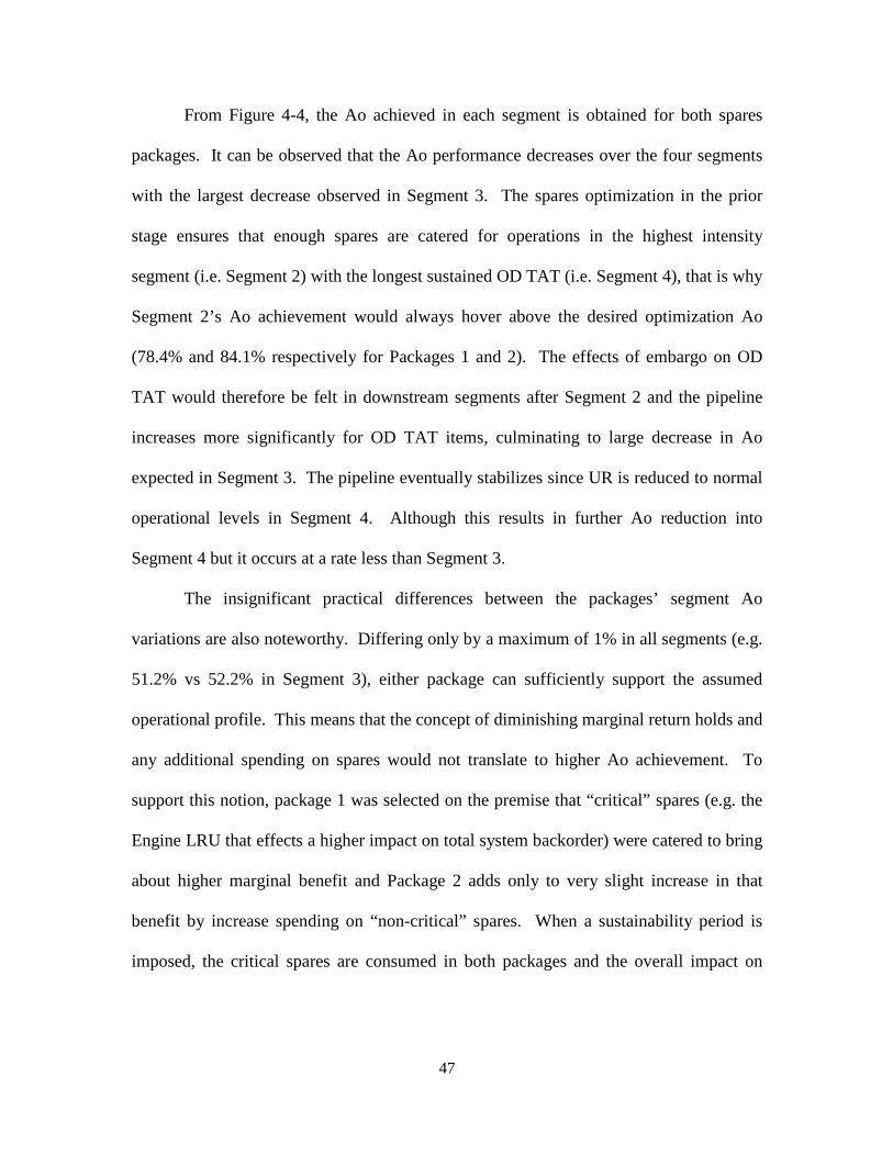
Figure 4-4. Sustainability Analyses of Spares Packages
47
From Figure 4-4, the Ao achieved in each segment is obtained for both spares
packages. It can be observed that the Ao performance decreases over the four segments
with the largest decrease observed in Segment 3. The spares optimization in the prior
stage ensures that enough spares are catered for operations in the highest intensity
segment (i.e. Segment 2) with the longest sustained OD TAT (i.e. Segment 4), that is why
Segment 2’s Ao achievement would always hover above the desired optimization Ao
(78.4% and 84.1% respectively for Packages 1 and 2). The effects of embargo on OD
TAT would therefore be felt in downstream segments after Segment 2 and the pipeline
increases more significantly for OD TAT items, culminating to large decrease in Ao
expected in Segment 3. The pipeline eventually stabilizes since UR is reduced to normal
operational levels in Segment 4. Although this results in further Ao reduction into
Segment 4 but it occurs at a rate less than Segment 3.
The insignificant practical differences between the packages’ segment Ao
variations are also noteworthy. Differing only by a maximum of 1% in all segments (e.g.
51.2% vs 52.2% in Segment 3), either package can sufficiently support the assumed
operational profile. This means that the concept of diminishing marginal return holds and
any additional spending on spares would not translate to higher Ao achievement. To
support this notion, package 1 was selected on the premise that “critical” spares (e.g. the
Engine LRU that effects a higher impact on total system backorder) were catered to bring
about higher marginal benefit and Package 2 adds only to very slight increase in that
benefit by increase spending on “non-critical” spares. When a sustainability period is
imposed, the critical spares are consumed in both packages and the overall impact on
48
system backorders is the same. As such, the systemic Ao reduction would be similar in
both cases, differing only by the slight effect of additional “non-critical” spares.
Overall, these observations allow analysts to critically examine the effort of
spares optimization to evaluate the impact on sustainability performance and better
position them in such inventory modeling domain knowledge. Both the optimization and
sustainability models must be utilized in synchronized mode to create better sense and
decision making in spares acquisition, trading between their costs, benefits and effects.
Model Run-Time Performance
With reference to Table 2-1 of the literature review section, one of OPUS10
limitations was the need for considerable effort in constructing the data and model inputs.
The objective in OPUS10 was to eliminate the need to understand the optimization
engine but this inevitably meant more time spent on customizing the information to a
form suitable for the software. In comparison, the NLP model provides the same
WYSIWYG platform for both data inputs and model construction. There is no
requirement to further manipulate the data as it is already entered in a form built for the
modeling phase. Although Solver run-time is not as comparable to the speed of OPUS10
analytical engine, the overall effort to conduct an analysis is substantially less. Table 4-1
summarizes the time comparison between the two platforms in carrying out optimization
studies:
49
Category Sequential tasks for a single analysis OPUS10 Model Analysis Time
(mins)
NLP Model Analysis Time
(mins)
Data Entry
Collate and manipulate input data in Excel 15 15
Convert input data to software input format 30 Nil
Modeling
Create / Modify existing software's operations and logistics profile model 25 15
Input of data into software 10 Nil
Results Output
Generate run results 5 15
Analyze results 5 5
Total Time Required 90 mins 50 mins
Table 4-1. Comparison of Time Required for OPUS10 and NLP Model Studies
With all the favourable observations and analyses of the output results, the NLP
model can be concluded as satisfactorily verified and validated for turnkey
implementation.
50
V. Conclusion and Recommendation
This chapter closes out the effort of this research. First, the objectives are re-
visited to ensure that the requirements have been met by the research outcomes. Second,
the significance of the effort is examined for its relevance in potential applications and
benefits in the RSAF’s context. Third, recommendations for action are proposed so that
follow-on implementation of the research model can be realized. Finally, the research
assumptions are reassessed to examine areas where future research can be explored.
Conclusion of Research
The objectives put forth at the start of this research were satisfactorily met. The
model provided an easy-to-use interface to simultaneously allow the handling of data
input and modeling interactions that ensure analysts are able to systematically step
through the modeling process. This logical flow also enables the model to customize
different maintenance support scenarios, making the solution versatile in its adaptation.
Accuracy was achieved by the ability to model variations of component VTMRs to better
represent all failure behaviors. These capabilities were realized through a model
designed with readily developed templates for dynamic operational profile conversion
and NLP optimization logic, allowing speedy analyses to be conducted. The outputs
provided insights on the most cost-effective spares proposal. Coupled with the
appreciation of spares performance over dynamically changing operations, the model
delivered the edge needed to conduct spares optimization and sustainability analyses for
O&S planning and contingency operations, which would otherwise be difficult in a
“black-box” software. Finally, the successful validation results culminated the basis for
practical deployment of the tool for implementation within the RSAF.
51
Significance of Research
This research is in tandem with AELO’s push towards seeking new, agile and
responsive logistics solutions to support an expanding RSAF’s force structure. As more
complex and sophisticated weapon systems are acquired, the requirements change to take
new forms and the maintenance support concepts have to be synchronized to better
sustain these operations. The optimization/sustainability model developed in this
research provides a versatile platform to provide this edge in inventory modeling. It was
designed around inventory modeling fundamentals and can be easily adapted to study
different reparable maintenance scenarios. The analysts need only modify the model
structures to best suit the problem on hand, but the computations are similar. This was
possible due to the strength of the WYSIWYG design interface. Moreover, because of
this design principle, the analysts are equipped with the tool necessary to deepen their
competencies in supply chain management expertise within the inventory-modeling
domain. They will be able to conduct swift, accurate and credible inventory spares
analyses to support O&S and Contingency operations and hence expand expertise on
spares planning for future operating concepts, grounding their knowledge to meet the
engineering demand in the Third Generation RSAF.
Recommendations for Action
The research model was developed on a representative set of aircraft sub-system
components. The next stage would be to implement a turnkey version to include all
components. The 6-steps process of model development, explained in Chapter 3, will
logically step the analyst through the model deployment, as it would be done in actual
implementation of any optimization and sustainability studies. Further validation should
52
be conducted, both with OPUS10 and with actual field data (actual component VTMRs
and spares utilization rates over time) to solidify the implementation of the model. Once
that is achieved, the model can be deployed in contingency operations planning to carry
out analyses and real-time performances would aid to improve and modify the model in
areas like modeling structures and planning parameters. Subsequent rollout of the model
on all aircraft platforms will eventually see widespread adoption and unique
modifications tailored to support aircraft-specific maintenance scenarios.
Recommendations for Future Research
Some of the assumptions made in Chapter 2 can be relaxed to develop areas
where future research can be explored. First, the assumption of an in-country fighter fleet
can be expanded to include various operating sites. The model can be tailored to
compute the unique pipeline characteristics that individual sites experience and the spares
optimization can be conducted for each site. The overall fleet availability is then
aggregated from these individual site performances. However, the behavior of the model
needs to be studied further if such expansion can be accommodated while sustaining run-
time and accuracy of analysis. Second, while this research assumes Ao performance is
affected only by the cost of spares, the variability of other maintenance factors (e.g.
MTTR manpower constraints and cannibalization effects) and logistics parameters (e.g.
OST and lateral base support) can be studied further to generate more systemic measures
on the total effect on operational performance. Third, corrective maintenance MTBF is
assumed the driving factor behind the demand rates in the model. The study can be
expanded to explore the effects of preventive maintenance policies and how that affects
the overall optimization. The resulting stock levels may be used to assess the viability of
53
conducting preventive maintenance in the sustainability period. Finally, the sustainability
analysis portion of the model is an analytical solution and provides a fixed Ao
performance metric in each individual segment. However, better fidelity of the Ao on a
per unit time basis (e.g. day to day) will better track the time-varying performance and
not be confined as a segment metric. This is especially crucial and valuable for decision-
making in time-sensitive operations. To deliver this capability, Monte Carlo simulation
can be utilized in a secondary model to collect unit time status of spares consumption and
backorders count as the aircraft system is subjected to varying utilization; and
accordingly the sustainability analysis can be made to output Ao variation over time.
54
Appendix A
Spares Data
55
Appendix B
Combined Spares Data and Logistics Parameters (Propulsion System Excerpt)
56
Appendix C
Dynamic Operational Profile Conversion Model (4-segment Sustainability Period)
57
58
59
Appendix D
Item Backorders and System Performance Computations (Propulsion System)
60
61
Appendix E
Excel VBA® Macro Programming Scripts
EBO and VBO for Poisson Distribution: Public Function EBOPOISSON(Mean As Double, Stock As Integer) As Double EBOPOISSON = Mean - Stock For x = 0 To Stock EBOPOISSON = EBOPOISSON + (Stock - x) * Application.WorksheetFunction.Poisson(x, Mean, False) Next x End Function Public Function VBOPOISSON(Mean As Double, Stock As Integer) As Double VBOPOISSON = 0 For x = (Stock + 1) To 999 VBOPOISSON = VBOPOISSON + ((x - Stock) ^ 2) * Application.WorksheetFunction.Poisson(x, Mean, False) Next x VBOPOISSON = VBOPOISSON - (EBOPOISSON(Mean, Stock) ^ 2) End Function
62
EBO and VBO for Binomial Distribution: Public Function EBOBINOM(Mean As Double, Stock As Integer, VTMR As Double) As Double n = Application.WorksheetFunction.RoundDown(((Mean / (1 - VTMR)) + 0.99), 0) p = Mean / n EBOBINOM = Mean - Stock For x = 0 To Stock EBOBINOM = EBOBINOM + (Stock - x) * Application.WorksheetFunction.BinomDist(x, n, p, False) Next x End Function Public Function VBOBINOM(Mean As Double, Stock As Integer, VTMR As Double) As Double n = Application.WorksheetFunction.RoundDown(((Mean / (1 - VTMR)) + 0.99), 0) p = Mean / n VBOBINOM = 0 For x = (Stock + 1) To n VBOBINOM = VBOBINOM + ((x - Stock) ^ 2) * Application.WorksheetFunction.BinomDist(x, n, p, False) Next x VBOBINOM = VBOBINOM - (EBOBINOM(Mean, Stock, VTMR) ^ 2) End Function
63
EBO and VBO for Negative Binomial Distribution: Public Function COMBINATIO(a, x) As Double If (x = 0) Then COMBINATIO = 1 ElseIf (x = 1) Then COMBINATIO = a ElseIf (x = 2) Then COMBINATIO = ((a + x - 1) * a) / Application.WorksheetFunction.Fact(x) ElseIf (x = 3) Then COMBINATIO = ((a + x - 1) * (a + x - 2) * a) / Application.WorksheetFunction.Fact(x) ElseIf (x = 4) Then COMBINATIO = ((a + x - 1) * (a + x - 2) * (a + x - 3) * a) / Application.WorksheetFunction.Fact(x) ElseIf (x = 5) Then COMBINATIO = ((a + x - 1) * (a + x - 2) * (a + x - 3) * (a + x - 4) * a) / Application.WorksheetFunction.Fact(x) ElseIf (x = 6) Then COMBINATIO = ((a + x - 1) * (a + x - 2) * (a + x - 3) * (a + x - 4) * (a + x - 5) * a) / Application.WorksheetFunction.Fact(x) ElseIf (x = 7) Then “Recursive”, continue to cover till x = 50 Else End…. End If End Function Public Function EBONEGBINOM(Mean As Double, Stock As Integer, VTMR As Double) As Double a = Mean / (VTMR - 1) b = (VTMR - 1) / VTMR EBONEGBINOM = Mean - Stock For x = 0 To Stock EBONEGBINOM = EBONEGBINOM + (Stock - x) * ((COMBINATIO(a, x)) * (b ^ x) * ((1 - b) ^ a)) Next x End Function
64
Public Function VBONEGBINOM(Mean As Double, Stock As Integer, VTMR As Double) As Double a = Mean / (VTMR - 1) b = (VTMR - 1) / VTMR VBONEGBINOM = 0 For x = (Stock + 1) To 50 VBONEGBINOM = VBONEGBINOM + ((x - Stock) ^ 2) * ((COMBINATIO(a, x)) * (b ^ x) * ((1 - b) ^ a)) Next x VBONEGBINOM = VBONEGBINOM - (EBONEGBINOM(Mean, Stock, VTMR) ^ 2) End Function
65
Appendix F
Non-Linear Programming Logic
Logic: Microsoft Excel Solver® Setup:
66
Appendix G
NLP Poisson Model vs OPUS Model Data Output
VTMR = 1 for all items
67
Appendix H
OPUS Model Cost-Effectiveness Output
68
Bibliography
Adams, J. L., Abell, J. B., & Isaacson, K. E., 1993, Modeling and Forecasting the Demand for Aircraft Recoverable Spare Parts, pp. 7, 26 & 27, DTIC. Retrieved from http://www.dtic.mil/cgi-bin/GetTRDoc?Location=U2&doc=GetTRDoc.pdf&AD=ADA282492 AELO (Air Engineering and Logistics Organisation), 2012, Provisioning and Procurement Policy, Vol. 302.11.003, pp. 1-4. Banks, J., Carson, J., Nelson, B., Nicol, D. (2010), Discrete-Event System Simulation, pp. 34-39, 5th Edition, Pearson Education. Blazer, D. J., & Sloan, J. D., 2007, Logistics Support: Relating Readiness to Dollars, Air Force Journal of Logistics, Vol. 31, Issue 2, pp. 67-68. Retrieved from http://go.galegroup.com/ps/i.do?id=GALE%7CA169715720&v=2.1&u=fl3319&it=r&p=SPJ.SP00&sw=w DISO (Defence Industry and Systems Office), 2009, MINDEF Life Cycle Management Manual, LCM-III-4-HDBK (Amendment no. 1.0), ILS Handbook, pp. 5-1 to 5-5 and 10-1 to 10-2. Feeney, G. J., & Sherbrooke, C. C., 1966, The (s-1, s) Inventory Policy under Compound Poisson Demand, Management Science, Vol. 12, Issue 5, pp. 391-411. Retrieved from http://mansci.journal.informs.org/content/12/5/391.short Frontline Systems Inc., 2010, Premium Solver Platform for Mac, User Guide, Version 10.5, pp. 15. Retrieved from http://www.solver.com/system/files/access/PremiumSolverPlatformforMac_0.pdf Graves, S. C., 1985, A Multi-Echelon Inventory Model for a Repairable Item with One-for-One Replenishment, Management Science, Vol. 31, Issue 10, pp. 1247-1256. Retrieved from http://mansci.journal.informs.org/content/31/10/1247.short Gross, D., 1982, On the Ample Service Assumption of Palm's Theorem in Inventory Modeling, Management Science, Vol. 28, Issue 9, pp. 1065-1079. Retrieved from http://mansci.journal.informs.org/content/28/9/1065.short Gross, D., Miller, D. R., & Soland, R. M., 1983, A Closed Queueing Network Model for Multi-Echelon Repairable Item Provisioning, IIE Transactions, Vol. 15, Issue 4, pp. 344-352. Retrieved from http://www.tandfonline.com/doi/abs/10.1080/05695558308974658 MINDEF (Ministry of Defence, Singapore), 2009, Military Domain Experts Scheme Guidebook., pp. 8. Retrieved from http://www.mindef.gov.sg/imindef/press_room/clarification/20jul11_clarification.html
Muckstadt, J. A., 1973, A Model for a Multi-Item, Multi-Echelon, Multi-Indenture Inventory System, Management Science, Vol. 20, Issue 4, Part I, pp. 472-481. Retrieved from http://mansci.journal.informs.org/content/20/4-Part-I/472.short Ng, C. M., 2012, Reflections 2: Practical Aspects of Leadership, Leading in the Third Generation SAF, Pointer Monograph no. 9, pp. 36. Retrieved from http://www.mindef.gov.sg/imindef/publications/pointer/monographs/mono9.html O'Malley, T. J., 1983, The Aircraft Availability Model: Conceptual Framework and Mathematics, Logistics Management Institute, pp. 1-3. Retrieved from http://www.dtic.mil/dtic/tr/fulltext/u2/a132927.pdf Seila, A. F., 2005, Spreadsheet Simulation, Proceedings of the 2005 Winter Simulation Conference, WSC '05, pp. 33-40. Retrieved from http://www.informs-sim.org/wsc05papers/005.pdf Sherbrooke, C. C., 1968, METRIC: A Multi-Echelon Technique for Recoverable Item Control, Operations Research, Vol. 16, Issue 1, pp. 122-141. Retrieved from http://or.journal.informs.org/content/16/1/122.short Sherbrooke, C. C., 1986, VARI-METRIC: Improved Approximations for Multi-Indenture, Multi-Echelon Availability Models, Operations Research, Vol. 34, Issue 2, pp. 311-319. Retrieved from http://or.journal.informs.org/content/34/2/311.short Sherbrooke, C. C., 2004, Optimal Inventory Modeling of Systems: Multi-Echelon Techniques, 2nd Edition, Vol. 72, International Series in Operations Research & Management Science, Kluwer Academic Publishers. Retrieved from http://books.google.com/books?id=FTHA4HKBzLwC Slay, F.M., Bachman, T.C., Kline R.C., O'Malley, T.J., Eichorn, F.L., King, R.M., 1996, Optimizing Spares Support: The Aircraft Sustainability Model, pp. 1-3 to 1-6, Logistics Management Institute. Retrieved from www.dtic.mil/dtic/tr/fulltext/u2/a320502.pdf Systecon AB., 2007, Introducing OPUS10, Reference Guide, pp. 1-12. Retrieved from http://www.systecon.se/documents/Introducing_OPUS10.pdf Wolber, D., Su, Y., & Chiang, Y. T., 2002, Designing Dynamic Web Pages and Persistence in the WYSIWYG Interface, Proceedings of the 7th International Conference on Intelligent User Interfaces, pp. 228-229. Retrieved from http://delivery.acm.org/10.1145/510000/502770/p228-wolber.pdf?ip=129.92.250.40&id=502770&acc=ACTIVE%20SERVICE&key=C2716FEBFA981EF181036934DE0C3997E5DA8DA67DCD2AC9&CFID=235988845&CFTOKEN=87629846&__acm__=1374866416_2072838f3b607dcd4f366fd171331d20
Military Expert 5 (ME5 - Major equivalent) Edmund K.W. Pek is a Material
Acquisition Engineering Officer with the Republic of Singapore Air Force (RSAF). He
was enlisted as an F-5 Aircraft J85 Engine Senior Technician in August 1997. Following
officer conversion, he was commissioned in April 2000. ME5 Pek’s assignments in
maintenance squadrons include Officer-In-Charge (OIC) A-4 Skyhawk Maintenance
Section, Aircraft Maintenance Flight, Air Logistics Squadron, Tengah Air Base (2000 –
2004); and Deputy Officer Commanding (Dy OC) Maintenance Control Flight, Air
Logistics Squadron, Tengah Air Base (2004). Following his maintenance assignments,
he was awarded the Singapore Armed Forces (SAF) Academic Training Award (ATA) to
pursue a Mechanical Aerospace Engineering Degree in Nanyang Technological
University (NTU) of Singapore. Graduated with an Honours Bachelor degree, he was
assigned to Headquarters RSAF (HQ RSAF) in July 2007 as aircraft material acquisition
staff officer in Materials System Branch (MSB) of Air Engineering and Logistics
Department (ALD). Progressed to head the fighters/ transports/ air defence weapon
systems acquisition section in July 2010, he led the material acquisition program for the
F-35 Joint Strike Fighter platform. Subsequently, he was conferred the prestigious SAF
Postgraduate Award (SPA) in Jan 2012 to pursue double masters degrees in Defence
Technology and Systems (MDTS) in National University of Singapore (NUS) and
Logistics Supply Chain Management (LSCM) in the Air Force Institute of Technology
(AFIT), Wright-Patterson Air Force Base (WPAFB), United States Air Force. Following
graduation, he will be assigned to the Unmanned Aerial Vehicle Command (UC) as
Mechanical OC.
REPORT DOCUMENTATION PAGE Form Approved OMB No. 074-0188
The public reporting burden for this collection of information is estimated to average 1 hour per response, including the time for reviewing instructions, searching existing data sources, gathering and maintaining the data needed, and completing and reviewing the collection of information. Send comments regarding this burden estimate or any other aspect of the collection of information, including suggestions for reducing this burden to Department of Defense, Washington Headquarters Services, Directorate for Information Operations and Reports (0704-0188), 1215 Jefferson Davis Highway, Suite 1204, Arlington, VA 22202-4302. Respondents should be aware that notwithstanding any other provision of law, no person shall be subject to an penalty for failing to comply with a collection of information if it does not display a currently valid OMB control number. PLEASE DO NOT RETURN YOUR FORM TO THE ABOVE ADDRESS. 1. REPORT DATE (DD-MM-YYYY)
15/09/2013 2. REPORT TYPE
Master’s Thesis 3. DATES COVERED (From – To)
01/10/2012 – 15/09/2013 4. TITLE AND SUBTITLE Development of Availability and Sustainability Spares Optimization Models for Aircraft Reparables
5a. CONTRACT NUMBER
5b. GRANT NUMBER 5c. PROGRAM ELEMENT NUMBER
6. AUTHOR(S) Pek, Edmund K.W., Major (Military Expert 5)
5d. PROJECT NUMBER 5e. TASK NUMBER 5f. WORK UNIT NUMBER
7. PERFORMING ORGANIZATION NAMES(S) AND ADDRESS(S) Air Force Institute of Technology Graduate School of Engineering and Management (AFIT/EN) 2950 Hobson Street, Building 642 WPAFB OH 45433-7765
8. PERFORMING ORGANIZATION REPORT NUMBER
AFIT-ENS-13-S-4
9. SPONSORING/MONITORING AGENCY NAME(S) AND ADDRESS(ES) Col. Lim Soon Chia Deputy Chief Research & Technology Officer (Ops)/(C4) Defence Research and Technology Office (DRTO) 303, Gombak Drive, Ministry of Defence, Singapore 669645 DID: +65-67683181; Email: [email protected]
10. SPONSOR/MONITOR’S ACRONYM(S)
MINDEF 11. SPONSOR/MONITOR’S REPORT NUMBER(S)
12. DISTRIBUTION/AVAILABILITY STATEMENT Distribution A. Approved for Public Release; Distribution Unlimited. 13. SUPPLEMENTARY NOTES 14. ABSTRACT The Republic of Singapore Air Force (RSAF) conducts Logistics Support Analysis (LSA) studies in various engineering and logistics efforts on the myriad of weapon systems. In these studies, inventory spares provisioning, availability and sustainability analyses are key focus areas to ensure asset sustenance. In particular, OPUS10, a commercial-off-the-shelf software, is extensively used to conduct reparable spares optimization in acquisition programs. However, it is limited in its ability to conduct availability and sustainability analyses of time-varying operational demands, crucial in Operations & Support (O&S) and contingency planning. As the RSAF seeks force structure expansion to include more sophisticated weapon systems, the operating environment will become more complex. Agile and responsive logistics solutions are needed to ensure the RSAF engineering community consistently pushes for deepening competencies, particularly in LSA capabilities. This research is aimed at the development of a model solution that combines optimization and sustainability capabilities to meet the dynamic requirements in O&S and contingency planning. In particular, a unique dynamic operational profile conversion model was developed to realize these capabilities. It is envisaged that the research would afford the ease of use, versatility, speed and accuracy required in LSA studies, to provide the necessary edge in inventory reparable spares modeling. 15. SUBJECT TERMS