REPRODUCIBILITY, DISTINGUISHABILITY, AND CORRELATION OF FIREBALL AND SHOCKWAVE DYNAMICS IN EXPLOSIVE MUNITIONS

DETONATIONS

THESIS

Bryan J. Steward, BS, Civilian

AFIT/GAP/ENP/06-19

DEPARTMENT OF THE AIR FORCE AIR UNIVERSITY

AIR FORCE INSTITUTE OF TECHNOLOGY

Wright-Patterson Air Force Base, Ohio

APPROVED FOR PUBLIC RELEASE; DISTRIBUTION UNLIMITED

The views expressed in this thesis are those of the author and do not reflect the official policy or position of the United States Air Force, Department of Defense, or the United States Government.

AFIT/GAP/ENP/06-19

REPRODUCIBILITY, DISTINGUISHABILITY, AND CORRELATION OF FIREBALL AND SHOCKWAVE DYNAMICS IN EXPLOSIVE MUNITIONS

DETONATIONS

THESIS

Presented to the Faculty

Department of Engineering Physics

Graduate School of Engineering and Management

Air Force Institute of Technology

Air University

Air Education and Training Command

In Partial Fulfillment of the Requirements for the

Degree of Master of Science (Applied Physics)

Bryan J. Steward, BS

Civilian

March 2006

APPROVED FOR PUBLIC RELEASE; DISTRIBUTION UNLIMITED

AFIT/GAP/ENP/06-19

REPRODUCIBILITY, DISTINGUISHABILITY, AND CORRELATION OF FIREBALL AND SHOCKWAVE DYNAMICS IN EXPLOSIVE MUNITIONS

DETONATIONS

Bryan J. Steward, BS Civilian

Approved:

\\Signed\\ ________ Glen P. Perram (Chairman) date

\\Signed\\ ________ Ronald F. Tuttle (Member) date

\\Signed\\ ________ Dave Bunker (Member) date

iv

AFIT/GAP/ENP/06-19

Abstract

The classification of battlespace detonations, specifically the determination of

munitions type and size using temporal and spectral features of infrared emissions, is a

particularly challenging problem. The intense infrared radiation produced by the

detonation of high explosives is largely unstudied. Furthermore, the time-varying fireball

imagery and spectra are driven by many factors including the type, size and age of the

chemical explosive, method of detonation, interaction with the environment, and the

casing used to enclose the explosive. To distinguish between conventional military

munitions and improvised or enhanced explosives, the current study investigates fireball

expansion dynamics using high speed, multi-band imagery. Instruments were deployed

to three field tests involving improvised explosives in howitzer shells, simulated surface-

to-air missiles, and small caliber muzzle flashes. The rate of shockwave expansion for the

improvised explosives was determined from apparent index of refraction variations in the

visible imagery. Fits of the data to existing drag and explosive models found in the

literature, as well as modifications to these models, showed agreement in the near- and

mid-fields (correlation coefficient, r2 > 0.985 for t < 50 msec); the modified models

typically predicted the time for the shockwave to arrive a kilometer away to better than

10%; and fit parameters typically had an uncertainty of less than 20%. The shockwave

was distinctive (Fisher Ratio, FR > 1) within the first 2-10 milliseconds after detonation,

then it decayed to an indistinguishable acoustic wave (coefficient of variation, CV < 0.05).

The area profiles of the fireballs were also examined and found to be highly variable,

especially after 10 milliseconds (CV > 0.5), regardless of munitions type. Scaling

v

relationships between properties of the explosive (mass, specific energies, and theoretical

energies) and detonation areas, characteristic times, and properties of the shockwave

were assessed for distinguishing weights and types: Efficiency decreased with mass (FR

> 19); early-time Mach number and overpressure were primarily dependent on energy

release (FR ~ 1.5-10); fireball area increased cubically with specific energies (r2 ~ 0.3-

0.76) but its time of occurrence decreased cubically (r2 ~ 0.4-0.67). The relationship

between fireball and shockwave features was fairly independent of variability (r2 ~ 0.5-

0.9), indicating that both fireball and shockwave features scale similarly with variability

in detonations.

vi

Acknowledgments

I would like to sincerely thank my faculty advisor, Dr. Glen Perram, for his

motivation and support. Throughout this research effort, his knowledge and experience

played a large role in guiding this work to completion. I would also like to thank the

members of my committee, Dr. Ron Tuttle and Dr. Dave Bunker, for their time and

guidance. I am appreciative of those who provided or supported data acquisition,

including Mark Houle and Greg Smith, and teams from NASIC, ATK Mission Research,

WPAFB’s 46th Test Wing, the Sensors Directorate’s Electro-optics Division, and TPL,

Inc. I am grateful for the guys in the Remote Sensing Lab (Kevin, Andy, Mike, Carl,

Randy, and Trevor) for making coming to work that much more enjoyable; and I am

especially thankful for all the times Kevin Gross has taken away from his research to

assist me in mine. I would also like to express gratitude to Amanda for her assistance. I

appreciate ASEE’s and the ARO’s support of my education and allowing me the

opportunity to pursue this work.

Finally, my deepest thanks go to my parents for their continual support,

encouragement, advice, and love. Without them, this would have been so much more

challenging than it already was.

Bryan J. Steward

vii

Table of Contents

Page

Abstract .............................................................................................................................. iv

Acknowledgments.............................................................................................................. vi

List of Figures .................................................................................................................... ix

List of Tables .................................................................................................................. xxii

List of Abbreviations and Symbols................................................................................ xxvi

List of Subscripts, Superscripts, and Suffixes .................................................................xxx

I. Introduction ..................................................................................................................1

Background..............................................................................................................1 Problem Statement ...................................................................................................2 Research Focus ........................................................................................................3 Investigative Questions............................................................................................4 Methodology............................................................................................................6 Assumptions/Limitations .........................................................................................7 Implications..............................................................................................................8

II. Theory ..........................................................................................................................9

Chapter Overview ....................................................................................................9 Combustion Chemistry ............................................................................................9 TNT........................................................................................................................12 RDX .......................................................................................................................13 Composition B .......................................................................................................14 Simple Theory of an Ideal Detonation...................................................................15 Shock Relations .....................................................................................................16 Shock Expansion....................................................................................................17 Explosive Model ....................................................................................................20 Drag Model ............................................................................................................22 Statistical Metrics...................................................................................................23 Summary ................................................................................................................26

III. Methodology ..............................................................................................................28

Chapter Overview ..................................................................................................28 Instrumentation ......................................................................................................29 Field Tests..............................................................................................................31 Data Extraction ......................................................................................................38 Data Processing......................................................................................................41 Area Profiles ..........................................................................................................43 Combustion Features .............................................................................................49

viii

Shock Expansion Models.......................................................................................51 Shock Expansion Fits.............................................................................................54 Shockwave Features...............................................................................................55 Feature Analysis.....................................................................................................58 Summary ................................................................................................................62

IV. Analysis and Results ..................................................................................................63

Chapter Overview ..................................................................................................63 Reproducibility of Area Profiles............................................................................64 Reproducibility of Fireball Features ......................................................................67 Shockwave Fits ......................................................................................................73 Reproducibility and Physicality of Shockwave Fit Parameters.............................78 Reproducibility of Temporal Shockwave Features................................................82 Distinguishability of Combustion Classes and Simple Types ...............................87 Distinguishability of Explosive Munitions ............................................................91 Correlation of Munitions Characteristics with Extracted Features........................98 Correlation of Fireball Features with Shockwave Features.................................108 Summary ..............................................................................................................114

V. Conclusions and Recommendations.........................................................................116

Chapter Overview ................................................................................................116 Previous Work .....................................................................................................117 Conclusions..........................................................................................................118 Recommendations for Future Work.....................................................................123 Summary ..............................................................................................................126

Appendix 1: Instrument Settings .....................................................................................128

Appendix 2: Fit Parameters .............................................................................................132

Bibliography ....................................................................................................................136

Vita ..................................................................................................................................139

ix

List of Figures

Figure Page

1. Internal energy is plotted as a function of reaction coordinate. As the

reaction proceeds (left to right), the reactants overcome the activation

energy, Ea, and are converted to products with a lower internal energy.

The process is typically a two step process: detonation is where the

reactants are converted to intermediate products with the oxygen present

in the system, releasing some energy, ∆HD. As additional oxygen is

introduced, the reaction continues and additional energy is released, ∆HA.

The total excess energy released is known as the heat of combustion, ∆HC. ........10

2. TNT molecular structure........................................................................................12

3. RDX molecular structure. ......................................................................................14

4. The scaled distance is plotted as a function of overpressure for a

detonation shockwave............................................................................................19

5. The distributions of values (x) for five sets of data are shown in the upper

plot. The mean (•) and standard deviation (I) of each set is offset to the

right of the data points. The lower plot shows the coefficient of variation

for each set of data. A CV value of ~0.5 or greater indicates large

variability of the data, whereas a value of ~0.1 or less indicates decent

reproducibility........................................................................................................24

6. Two sets of Gaussian distributed data are shown. Data points from set one

(○) have a distribution represent by the solid line. Data points from set

two (∆) have a distribution represent by the dotted line. From top to

x

bottom, the widths of the Gaussians (variability in the data sets) increase.

The resulting overlap in the distributions causes a decrease in separability,

as indicated by the lower Fisher Ratio. Decease in the FR will also occur

if the variability remains fixed but the means become closer together..................25

7. Correlation of two sets of data points, x and y, is shown. Complete

correlation 1r = (upper left) through poor correlation (lower right) can be

seen. .......................................................................................................................26

8. Relative spectral response of InGaAs FPA in the Indigo Alpha NIR

imager. ...................................................................................................................31

9. 155mm Composition B shell, 155mm TNT shell, and 105mm TNT shell

(left to right) detonated during the Bronze Scorpio field tests...............................32

10. Bronze Scorpio test layout. Both instrumentation sites were located above

ground zero, approximately 1100 meters away. ....................................................33

11. Dual Thrust Smokey SAM test setup at Wright Patterson AFB, Area B

Test Range. The DTSS was fixed approximately 1.5 meters above a

concrete runway. ....................................................................................................35

12. Muzzle Flash Test setup geometry ........................................................................37

13. Static image of a Bronze Scorpio detonation with its shockwave (left) and

the same image after image processing (right). The index change due to

the shockwave is difficult to see in the original image, but with

background subtraction and contrast adjustment, it can be seen as a nearly

spherical shell propagating away from the detonation. .........................................40

xi

14. Detonation fireball as seen from the Indigo Alpha NIR imager’s full field

of view (left) and the cropped image (right). .........................................................41

15. Detonation fireball as viewed by the Phantom camera in the red (upper

left), green (upper right), and blue (lower left) bands. Due to the

brightness of the smoke and debris in the blue band, the blue image was

masked (lower right) so that only hot fireball pixels would be seen. The

mask was based on hot pixels in the red band, with a ten pixel buffer on

each side.................................................................................................................42

16. The MWIR histogram of a Bronze Scorpio detonation event (left),

representative of all Bronze Scorpio events, shows excellent separation

between dark pixels and hot pixels. The temporal histogram of a typical

DTSS in the NIR (right) also exhibits separation between background and

hot pixels, but the distributions are wider. This is indicative of a wide

range of intensity levels in the combustion event, and can be attributed to

reflection from gases and surroundings. ................................................................44

17. The histogram as a function of time shows a minima near DN 3000.

Setting the threshold here (dashed line) assumes that all DNs above this

level are due to combustion emissions and that all DNs below this are due

to background or reflected light. ............................................................................45

18. NIR histograms (left) for the corresponding frame of the combustion even

(right). From top to bottom, the events are a muzzle flash, DTSS plume,

and afterburn fireball. The gray shading in the histogram corresponds to

xii

the average background, and the black shading corresponds to the DNs of

the event. The threshold levels are indicated with a dashed line. .........................46

19. The MWIR area profile of Bronze Scorpio event 26 is relatively

independent of the threshold level. Changing the threshold from 20% of

the dynamic range through 90% changes only the magnitude of the area,

but not its shape as a function of time. The scaling factors, S, for each

threshold level, th, are indicated below the plots...................................................47

20. The five area profiles are plotted for a Bronze Scorpio event in the red

band. Threshold area (solid dark line) is several orders of magnitude

below the maximum static (dotted dark like) and maximum dynamic

(dotted gray line) areas. The three sigma static profile (dashed dark line)

predicts the largest area, but the three sigma dynamic area (dashed gray

line) has a much lower magnitude. ........................................................................49

21. Threshold area profile as a function time for a Bronze Scorpio detonation

in the red band. The features that may be extracted from the profile are

indicated.................................................................................................................50

22. The area profiles for all erect 155mm TNT detonations are shown (thin

line) with their mean (thick line) and standard deviation (shaded region) in

the upper plot. The CV as a function of time for the area profiles is shown

on bottom. The mean CV value for the six events of this type’s feature is

1.22.........................................................................................................................64

23. The area profiles for all TNT detonations are shown (thin line) with their

mean (thick line) and standard deviation (shaded region) in the upper plot.

xiii

The CV as a function of time for the area profiles is shown on bottom. The

mean CV value for the thirteen events of this type’s feature is 1.6. .......................65

24. The area profiles for all Composition B detonations are shown (thin line)

with their mean (thick line) and standard deviation (shaded region) in the

upper plot. The CV as a function of time for the area profiles is shown on

bottom. The mean CV value for the five events of this type’s feature is

1.58.........................................................................................................................66

25. The area profiles for all TNT and Composition B detonations are shown

(thin line) with their mean (thick line) and standard deviation (shaded

region) in the upper plot. The CV as a function of time for the area profiles

is shown on bottom. The mean CV value for the eighteen events of this

type’s feature is 1.98. .............................................................................................67

26. The time to the peak detonation area in the red band is shown for each

event (thin bars) of the eleven munitions groups. The mean feature value

is also shown for each group (wide bars) and the value is indicated below

the top plot. The bottom plot shows the coefficient of variation for the

feature in each group. detredt is a very reproducible feature for all groups,

indicating it may be a feature common to explosives in general. ..........................70

27. The peak detonation area in the blue band is shown for each event of the

eleven munitions groups (thin bars). The mean feature value is also

shown for each group (wide bars) and the value is indicated below the top

plot. The bottom plot shows the coefficient of variation for the feature in

xiv

each group. For TNT, detblueA shows correlation for a single weight and

may be a good feature for classification. ...............................................................70

28. The time required for the fireball’s area to fall below the noise level in the

NIR is shown for each event of the eleven munitions groups (thin bars).

The mean feature value is also shown for each group (wide bars) and the

value is indicated below the top plot. The bottom plot shows the

coefficient of variation for the feature in each group. ...........................................72

29. The time required for the fireball’s area to fall below the noise level in the

MWIR is shown for each event of the eleven munitions groups (thin bars).

The mean feature value is also shown for each group (wide bars) and the

value is indicated below the top plot. The bottom plot shows the

coefficient of variation for the feature in each group. ...........................................72

30. Position of the shockfront (•) is shown with its uncertainty for an erect

155mm TNT detonation. The shock fit (solid line), modified shock fit

(dashed line), and shock 350 fit (dotted line) are also shown. The

functions were fit to the early-time data (lower left) with the late-time data

point used to evaluate the fits in the far-field (upper right). ..................................74

31. Position of the shockfront (•) is shown with its uncertainty for an erect

155mm TNT detonation. The drag fit (solid line), modified drag fit

(dashed line), and drag 350 fit (dotted line) are also shown. The functions

were fit to the early-time data (lower left) with the late-time data point

used to evaluate the fits in the far-field (upper right). ...........................................75

xv

32. The coefficient of determination calculated from the near, mid, and early

far-field shockwave positions, is shown for each fit function and all events

(top). The deviation of the fit from the far-field data point is also shown

(below). All of the fits show good correlation in early-time data, but in the

far-field the shock 350 and drag 350 models show the best agreement with

observations. ..........................................................................................................77

33. The speed of sound fit parameter for the modified drag (dark bars) and

modified shock (light bars) fit functions are plotted for each event of each

type in the upper plot. The shaded region was the average range of speeds

of sound (based on the temperature) for the Bronze Scorpio field tests. On

the lower plot, the Coefficients of Variation are plotted for the fit

parameter by type. The modified drag best-fit speed of sound was

consistently high whereas the modified shock best-fit speed of sound was

consistently low. ....................................................................................................78

34. The characteristic radius from the drag 350 fit function is shown for each

event of the eleven munitions groups (thin bars). The mean feature value

is also shown for each group (wide bars) and the value is indicated below

the top plot. The bottom plot shows the coefficient of variation for the

feature in each group. The reproducibility of 350draga for munitions types

indicates that it is representative of a feature of the munitions, and perhaps

will be useful in classification................................................................................81

35. The time exponent fit parameter from the explosive fit function is shown

for each event of the eleven munitions groups (thin bars). The mean

xvi

feature value is also shown for each group (wide bars) and the value is

indicated below the top plot. The bottom plot shows the coefficient of

variation for the feature in each group. This feature is very reproducible

for all groups yet increases for multiple munitions groups, indicating

potential for classification......................................................................................82

36. The mean Mach number as a function of time (solid line) with the

corresponding standard deviation (shaded region) for the modified drag fit

to the shockwave is shown in the upper plot for all TNT and Composition

B events The lower plot shows the coefficient of variation for each time

step. ........................................................................................................................85

37. The mean shock pressure as a function of time (solid line) with the

corresponding standard deviation (shaded region) for the modified drag fit

to the shockwave is shown in the upper plot for all TNT and Composition

B events The lower plot shows the coefficient of variation for each time

step. ........................................................................................................................85

38. The mean detonation energy predicted at each time step (solid line) with

the corresponding standard deviation (shaded region) for the modified

drag fit to the shockwave is shown in the upper plot for all TNT and

Composition B events The lower plot shows the coefficient of variation

for each time step. ..................................................................................................86

39. The time required for the area to fall to the noise level (in the NIR) is

plotted for all detonations (○) DTSS plumes (∆) and muzzle flashes (□).

The upper plot shows the data points assuming normal distributions

xvii

(detonations are represented by the solid line, plumes by the dotted line,

and muzzle flashes by the dashed line). The lower plot represents the

probability that a given time will be one of the three combustion classes,

based on the normal distributions. Those events whose group has a higher

probability are classified correctly (•) and those whose group has a lower

probability are classified incorrectly (x). ...............................................................88

40. The peak area (in the NIR) is plotted for all detonations (○) DTSS plumes

(∆) and muzzle flashes (□). The upper plot shows the data points

assuming normal distributions (detonations are represented by the solid

line, plumes by the dotted line, and muzzle flashes by the dashed line).

The lower plot represents the probability that a given area will be one of

the three combustion classes, based on the normal distributions. Those

events whose group has the highest probability are classified correctly (•)

and those whose group has a lower probability are classified incorrectly

(x)...........................................................................................................................89

41. The peak area (in the NIR) is plotted for all conventional (○) novel (∆)

and novel FMJ (□) muzzle flashes. The upper plot shows the data points

assuming normal distributions (conventional are represented by the solid

line, novel by the dotted line, and novel FMJ by the dashed line). The

lower plot represents the probability that a given area will be one of the

three muzzle flash types, based on the normal distributions. Those events

whose group has the highest probability are classified correctly (•) and

those whose group has a lower probability are classified incorrectly (x)..............91

xviii

42. The efficiency of detonation at 14.8 msec (from the modified drag model)

is plotted for all 105mm TNT (○) and Composition B (∆) detonations.

The upper plot shows the data points assuming normal distributions,

where 105mm TNT is represented by the solid line and Composition B by

the dotted line. The lower plot represents the probability that a given

efficiency will be one munitions group or the other, based on the normal

distributions. Those events whose group has a higher probability are

classified correctly (•) and those whose group has a lower probability are

classified incorrectly (x). The FR is 103...............................................................94

43. The energy of detonation at 14.8 msec (from the modified drag model) is

plotted for all 105mm TNT (○) and Composition B (∆) detonations. The

upper plot shows the data points assuming normal distributions, where

105mm TNT is represented by the solid line and Composition B by the

dotted line. The lower plot represents the probability that a given

efficiency will be one munitions group or the other, based on the normal

distributions. Those events whose group has a higher probability are

classified correctly (•) and those whose group has a lower probability are

classified incorrectly (x). The FR is 1.8314..........................................................95

44. The time to the peak fireball area (in the green band) is plotted for all TNT

(○) and Composition B (∆) detonations. The upper plot shows the data

points assuming normal distributions, where TNT is represented by the

solid line and Composition B by the dotted line. The lower plot represents

the probability that a given time will be one munitions group or the other,

xix

based on the normal distributions. Those events whose group has a higher

probability are classified correctly (•) and those whose group has a lower

probability are classified incorrectly (x). The FR is 2.28. ....................................96

45. The detonation area (in the red band) is plotted for all 155mm TNT (○)

and 105mm TNT (∆) detonations. The upper plot shows the data points

assuming normal distributions, where 155mm TNT is represented by the

solid line and 105mm TNT by the dotted line. The lower plot represents

the probability that a given area will be one weight or the other, based on

the normal distributions. Those events whose group has a higher

probability are classified correctly (•) and those whose group has a lower

probability are classified incorrectly (x). The FR is 5.25. ....................................97

46. Detonation efficiency is plotted against the afterburn and detonation

energies in the upper plots, heat of detonation (which follows the same

correlation as the specific afterburn energy) initial mass in the lower plots.

As all quantities increase, the efficiency decreases. ............................................101

47. The highest non-efficiency correlations are shown for each munition

characteristic. The Mach number tends to increase with mass and

afterburn energy, although correlation is poor. The decrease in Mach

number with detonation energy is due to the use of the drag model outside

of its intended field and is not physically accurate. The time to the peak

fireball area increases with the third power of the heat of detonation,

neglecting the outliers. .........................................................................................103

xx

48. The highest non-efficiency correlations are shown for each TNT and

Composition B characteristic. The Mach number tends to increase with

mass and afterburn energy, although correlation is poor. The decrease in

Mach number with detonation energy is due to the use of the drag model

outside of its intended field and is not physically accurate. The time to the

peak fireball area increases with the third power of the heat of detonation,

neglecting the outliers. In all cases, correlation is higher than when C-4

was included.........................................................................................................105

49. Efficiency is plotted against the two masses of TNT and the correlation is

shown. Because there were only two weights of TNT, this plot indicate

separation of the data more than correlation. However, the trend is

apparent and can be used as a scaling rule of thumb. ..........................................107

50. Selected comparisons of fireball and shockwave features are shown for

detonations of all munitions. In general, the fireball and shockwave

features have a greater degree of correlation with each other than with

munitions characteristics, as indicated by the higher coefficients of

determination. The trends in the data are also fairly evident. .............................111

51. Selected comparisons of fireball and shockwave features are shown for

detonations of TNT and Composition B munitions. The degree of

correlation is not significantly affected by excluding C-4, indicating that

the relationship between the fireball and shockwave is explosive

composition independent. ....................................................................................112

xxi

52. Selected comparisons of fireball and shockwave features are shown for

TNT detonations only. The correlation between the features is the highest

when only a single explosive composition is used and there are very clear

trends....................................................................................................................113

xxii

List of Tables

Table Page

1. Selected properties of TNT isomer 2-4-6 [18].......................................................13

2. Selected properties of RDX [18]............................................................................14

3. Test matrix for Bronze Scorpio. Data collected and examined are denoted

by a “Y”; data that have yet to be acquired by AFIT (not examined) are

denoted by an “X”..................................................................................................34

4. Test matrix for Muzzle Flash Tests indicating ammunition type, number of

rounds fired, and number of rounds acquired with the Indigo imager...................38

5. Threshold DN for each instrument used in the three field tests. In the

Muzzle Flash test, there were two thresholds. The first measured

everything above background and was variable for each event. It was set

where the background DN spike drop below 1% of its maximum value,

typically around DN 600. The second threshold quantized only the DNs

of the bright flash and was fixed............................................................................46

6. Features extracted from the afterburn fireball in each band, denoted by an

“x”. .........................................................................................................................51

7. Material properties are shown for each munition in the Bronze Scorpio

tests. These, along with the assumed atmospheric properties (also shown),

allowed the near- and far-field radii to be calculated. ...........................................52

8. Types used in analysis. “Y” indicates use as a stand-alone type, “X”

indicated that the type was not analyzed separately but was used in groups

with other types, and “N” indicates no analysis was performed on the type.........59

xxiii

9. Grouping of types for reproducibility, distinguishability, and correlation

analysis...................................................................................................................59

10. The groups to be compared using the Fisher Ration are shown for each set

of comparisons. These include comparing groups of all combustion

events, groups of muzzle flashes only, and groups of munitions

detonations only. ....................................................................................................61

11. The most reproducible fireball features and the corresponding Coefficients

of Variation are given for each group of combustion events.................................68

12. The most reproducible shockwave fit parameters and the corresponding

Coefficients of Variation are given for each group of munitions. .........................80

13. The most reproducible shockwave features in the near-and mid-fields

( 0 30t≤ ≤ msec) and the corresponding Coefficients of Variation are given

for each group of munitions. The time in milliseconds where the CV was a

minimum for the feature is indicated. ....................................................................83

14. The Fisher Ratios for all features used in comparing detonations, DTSS

plumes, and muzzle flashes are shown for each combination of

combustion event classes. ......................................................................................87

15. The Fisher Ratios for all features used in comparing muzzle flashes are

shown for each combination of ammunition types. ...............................................90

16. Fisher Ratios for highly reproducible fireball and shockwave features are

shown for comparisons of explosive type (TNT and Composition B) and

weight (155mm and 105mm TNT). .......................................................................92

xxiv

17. The highest Fisher Ratios for each comparison are shown. Only a single

physical quantity of each model is shown because they are all

transformations of the same data. When multiple bands or models had

similar values, the one with the largest FR is given and indicated by *.

For time-dependent features, the time is given is milliseconds. ............................94

18. The coefficient of determination, r2, is shown for the features of the

shockwave (highest 10) and fireball (highest 4) that are most highly

correlated with all of the munitions’ afterburn energy, detonation energy,

specific energy released in the afterburn, heat of detonation, and mass. HA

and HD were found to be redundant and are shown together.................................99

19. The markers used to designate munitions type in Figure 46 through Figure

52 are shown below. All types containing C-4 are designated with the

same marker because these types were not independently examined..................100

20. The coefficient of determination, r2, is shown for the features of the

shockwave (highest 10) and fireball (highest 4) that are most highly

correlated with all of the TNT and Composition B munitions’ afterburn

energy, detonation energy, specific energy released in the afterburn, heat

of detonation, and mass. HA and HD were found to be redundant and are

shown together. ....................................................................................................104

21. The coefficient of determination, r2, is shown for the features of the

shockwave (highest 10) and fireball (highest 4) that are most highly

correlated with all of the TNT munitions’ afterburn energy, detonation

xxv

energy, specific energy released in the afterburn, heat of detonation, and

mass......................................................................................................................106

22. The shockwave and fireball features that showed a moderate or greater

degree of correlation with munitions characteristics are shown. The

typical range of r2 values are given, with all munitions representing the

lower end and TNT representing the upper. The trend indicates how the

feature behaves with increases in the munitions characteristic. ..........................108

23. For each fireball feature, the most correlated shockwave feature from each

group (all munitions, TNT and Composition B, and TNT) is shown. The

time at which temporal features were evaluated is indicated in

milliseconds. ........................................................................................................109

24. The Phantom camera’s resolution, full field of view, integration time, and

framerate are given for each detonation event in the Bronze Scorpio tests.........129

25. The Indigo imager’s instantaneous field of view, focal length, and full

field of view are given for each detonation event in the Bronze Scorpio

tests. .....................................................................................................................130

26. Munitions groups .................................................................................................132

27. Drag model fit parameters and uncertainties. ......................................................132

28. Modified drag model fit parameters and uncertainties. .......................................133

29. Drag350 model fit parameters and uncertainties. ................................................133

30. Explosive model fit parameters and uncertainties. ..............................................134

31. Modified explosive model fit parameters and uncertainties. ...............................134

32. Explosive350 model fit parameters and uncertainties. ........................................135

xxvi

List of Abbreviations and Symbols

A .....................................................................................................................................area

3A σ ................................................................................. statistical area with dynamic mean

03A σ .......................................................................................statistical area with static mean

tA .................................................................................. area integrated with respect to time

maxA ............................................................................... maximum area with dynamic mean

0maxA .................................................................................... maximum area with static mean

detA ................................................................................................... peak area of detonation

pkA ................................................peak area of combustion (fireball, plume, muzzle flash)

pxA ........................................................................................ area of event viewed per pixel

thA ................................................................................................................... threshold area

satA ......................................................................................................saturation (flash) area

β ............................................................................................................................. drag rate

0c ......................................................................................................ambient speed of sound

Pc ......................................................................................specific heat at constant pressure

VC .....................................................................................................coefficient of variation

Vc ....................................................................................... specific heat at constant volume

D .......................................................................... detonation velocity, shockwave velocity

d ................................................................................................................ distance to target

DN.................................................................................................................. digital number

xxvii

maxDN ...........................................................................................maximum digital number

thDN ............................................................................................... threshold digital number

DTSS............................................................................................. dual-thrust smokey SAM

AE .......................................................................... energy released in the afterburn fireball

aE ...............................................................................................................activation energy

DE .........................................................................theoretical energy released in detonation

( )DE t .................................... observed energy released in detonation as a function of time

|D tE = .................... observed energy released in detonation evaluated at the indicated time

FFOV ..........................................................................................................full field of view

FMJ ..........................................................................................................full metal jacketed

FN ................................................................................................................... frame number

FR.......................................................................................................................Fisher Ratio

γ .............................................................................................ratio of specific heats, /P Vc c

H∆ ...........................................................................heat of reaction, enthalpy of formation

AH∆ ................................................................specific energy released in afterburn fireball

CH∆ ........................................................................................................heat of combustion

DH∆ ........................................... heat of detonation, specific energy released in detonation

IFOV .......................................................................................... instantaneous field of view

InGaAs ......................................................................................... Indium Gallium Arsenide

InSb........................................................................................................Indium Antimonide

IR............................................................................................................................... infrared

xxviii

LWIR ...................................................................................................... long-wave infrared

M .................................................................................................shockwave mach number

m ...................................................................................................................................mass

MWIR ......................................................................................................mid-wave infrared

N ....................................................................................................... total number of pixels

iN ..............................................................................number of pixels at ith digital number

n .......................................................................................... number of values in feature set

NIR....................................................................................................................near-infrared

0p ......................................................................................initial pressure, ambient pressure

1p ........................................................................................... final pressure, shock pressure

R ............................................................................. shockwave radius, shockwave position

maxR ..........................................................................................maximum shockwave radius

r ......................................................................................................... correlation coefficient

2r ..............................................................................................coefficient of determination

2r .................................................................................... mean coefficient of determination

RDX ......................................................................................Cyclotrimethylenetrinitramine

RGB .......................................................................................................red, green, and blue

ρ ................................................................................................................................density

s ................................................................................................................... scaled distance

SAM.....................................................................................................surface-to-air missile

,X Yσ σ ................................................................................ standard deviation of feature set

2 2,X Yσ σ ................................................................................................ variance of feature set

xxix

T ........................................................................................................................ temperature

t ..................................................................................................................................... time

10t ................................................................ time at which area falls below 10% of its peak

50t .......................................................time at which area falls below 50% of its peak value

dett .......................................................................... time at which the detonation area peaks

nt .......................................................................... time at which area falls to the noise level

pkt ......................................................................... time at which the combustion area peaks

TNT............................................................................................................... Trinitrotoluene

pxθ ............................................................ instantaneous field of view of instrument (pixel)

V ................................................................................................................................volume

,X Y ...................................................................................................................... feature set

,X Y ........................................................................................................mean of feature set

,i ix y ................................................................................................... ith value in feature set

ξ .............................................................................................................reaction coordinate

0ξ ............................................................................................................ numerical constant

xxx

List of Subscripts, Superscripts, and Suffixes

0 ...........................................................................................................initial condition/state

1 ..............................................................................................................final condition/state

blue ..........................................................................................................................blue band

CompB .............................................................................................................. Composition B

drag ....................................................................................................................... drag model

exp ......................................................................................................explosive/shock model

350drag ............................................................................................................ drag 350 model

exp350 ...........................................................................................explosive/shock 350 model

green .......................................................................................................................green band

mdrag ......................................................................................................modified drag model

expm .................................................................................... modified explosive/shock model

MWIR ................................................................................................. mid-wave infrared band

NIR ............................................................................................................near-infrared band

RDX ................................................................................................................................ RDX

red .............................................................................................................................red band

( )t ................................................................................................................function of time

|t= ...............................................................evaluated at the time indicated (in milliseconds)

TNT ..................................................................................................................................TNT

1

REPRODUCIBILITY, DISTINGUISHABILITY, AND CORRELATION OF

FIREBALL AND SHOCKWAVE DYNAMICS IN EXPLOSIVE MUNITIONS

DETONATIONS

I. Introduction

Background

The ability to remotely monitor and classify high explosive events that occur

around the world can be essential to the vital interests of the United States of America.

Furthermore the ability to distinguish between legitimate uses of high explosives (mining,

demolitions, construction, etc.) and the testing of enhanced or improvised weapons may

avert subsequent events with cataclysmic outcomes. Current technology allows optical

information from such events to be captured, but not enough is known about the

underlying physics of these events for the data obtained to allow discernment of exactly

what has occurred. Optical remote sensing is a growing field, but much work remains to

be done before identifying specific events based on the interpretation of the optical data

collected from remote sensing instruments is practical.

Optical remote sensing is the use of instruments or sensors to obtain the spectral

and spatial characteristics of target objects from a distance. It is used extensively for the

monitoring of static scenes such as crop growth, geological surveys, and urban patterns

[1][2][3], as well as faster transient events like forest fires [4][5]. Its range of use has

been from monitoring terrestrial events like the Kuwaiti oil fires [6][7] to collecting data

2

on extraterrestrial bodies light years away [8].

Remote sensing has also been used in military applications, for example, in

detecting missile launches [9][10], gun muzzle flashes [11][12] and explosive detonations

[13]. It is becoming increasingly important, however, not only to detect certain types of

events, but also to distinguish them – specifically high explosives. The ability to

distinguish a high explosives detonation from small arms fire or a missile plume, or to

take the classification a step further and allow munitions types to be uniquely identified

would give the war fighter a distinct tactical advantage.

Problem Statement

Currently, the ability to identify munitions types based on the remote sensing of

detonations is limited. While munitions may be distinguished with high confidence, this

is only true when enough a priori information is known [14]. The extent of a priori

information may be as minimal as knowing whether the munition was statically detonated

or air dropped, or it may be as specific as knowing the weight and casing. As the

understanding of detonations improves, however, superior classification features can be

chosen, and the extent of a priori information needed to classify the munitions type will

decrease.

Unfortunately, data collected from remote sensors result in hundreds of features

that may or may not correlate specifically with the type of event taking place or with the

specific explosive used. In order to choose the best features to classify munitions types,

it is important to understand how the features obtained from observation relate to

particular explosives. This can only be accomplished by developing phenomenological

3

relationships between the characteristics of the munitions (weight, casing, explosive

compound, etc.) and the detonation effects it produces, specifically the shockwave

immediately following detonation and the lingering afterburn fireball. In essence, a

phenomenological model of detonations is needed with identifiable specific correlatable

features that can be used to classify subsequent events.

Research Focus

High explosive detonations generate two major phenomena of interest; a

shockwave and an afterburn fireball. Identifying unique, correlatable signatures that

relate the detonation event to a classable munition is highly desirable. There is an

abundance of literature regarding the phenomenology of shockwaves for detonation

events [15][16][17]. This literature describes the pressure, velocity, energy, and extent of

shockwaves resulting from the initial detonation of an explosive material, which can be

difficult (but not impossible) to monitor optically. Furthermore, the detonation of an

explosive spans only a couple of milliseconds, making it difficult to identify; and

acquiring a temporal profile of the emissions is even more challenging. For practical

sensing of explosive detonations from aerial or spaced based platforms, it is the fireball

resulting from the afterburn (mixing of unburned reactants with atmospheric oxygen

resulting in explosive combustion) that is most easily monitored. The intense portion of

the afterburn spans hundreds of milliseconds, with the cooling fireball lingering for

seconds.

Thus improvements to the classification problem rely on understanding fireball

phenomenology, and while the aforementioned understanding of detonation shocks

4

exists, there is little understanding of the relationship between the initial characteristics of

the explosive and the resulting afterburn. There is much to be learned about these

relationships, including how the initial conditions affect the afterburn’s temperature

distribution, turbulent flow, emissivity, size, etc. It will be the properties that are most

easily remotely monitored, however, that may prove the most useful to the classification

problem, and the simplest properties that will provide for general understanding of

phenomenology. To this end, observations of fireball size as a function of time are an

ideal starting point – it is easily remotely observed and should have a direct relationship

to the characteristics of the munition type.

Additionally, because the shockwave resulting from a detonation of high

explosives is well understood and can be monitored optically, determining a

phenomenological relation between physical features that can be extracted from it

(velocity, pressure, etc.) and the explosive material characteristics should also be

possible. Furthermore, there is no clear connection between the characteristic features of

the shockwave and the behavior of the afterburn fireball. Examination of the

relationships between the shockwave and the fireball provides a great deal of insight into

the phenomenology of explosive munitions detonations and was a major focus of this

research.

Investigative Questions

Because detonation physics encompasses a wide range of subjects (the more

prominent fields including combustion chemistry, fluid flow, thermodynamics, and

spectral radiometry), it was necessary to narrow down the list of subjects that were

5

investigated by determining what specific questions needed to be answered. These were:

1. Which features are reproducible for munitions of the same type, yet

different for munitions of dissimilar types?

2. Which features of the shockwave and fireball are highly correlated with

characteristics of the explosive material?

3. How are features of the shockwave related to features of the afterburn

fireball?

The first question was important because the development of a phenomenological

understanding of detonations requires that the observations of the fireball and shockwave

be reproducible. Furthermore, for the understanding to be more than a characterization of

detonations in general there must be a noticeable difference in the fireball or shockwave

as the characteristics of the munitions change; i.e. features must be distinguishable.

Answering this question also served the practical purpose of aiding in the classification

problem, since classification of remotely sensed explosive detonations requires distinct,

reproducible signatures.

This led to the second question to be answered in this work. By identifying which

features are affected by changes in the explosive munitions’ characteristics, it was

possible to physically relate these features to those characteristics.

The final question answered was the major focus of this research. While the

fireball and shockwave resulting from explosive detonations were seemingly independent

of each other – the shockwave was supersonic ahead of the fireball and thus should not be

influenced by it – identifying which features were correlated helped to understand the

phenomenology of the features. High correlation between a feature of the shockwave and

6

one of the fireball indicated an underlying characteristic of the explosive material.

Having been found, they may be used as predictors of fireball and shockwave features.

Or, working the problem from the other end, classification may be accomplished by

relating observation of shockwave and fireball features to the originating explosive

material.

Methodology

This research was not approached from a purely theoretical standpoint; i.e. the

phenomenology was not developed from first principles. Rather, experimental

observations of explosive munitions detonations – and other combustion events (muzzle

flashes, missile plumes) for variety of data – were examined in several spectral bands.

Features of the fireball and the shockwave were extracted for the detonation events. The

majority of these features were physical in nature (i.e. the size of the fireball and the

velocity of the shockwave), which served to aid in developing phenomenological

relationships between the features and the explosive’s characteristics, as well as between

the features themselves. Other features, however, were extracted by fitting observed data

to theoretical models and using the fit parameters as features.

The extracted features of the fireball and shockwave were assessed in a number of

ways. They were examined for reproducibility for explosives of a single type,

distinguishability for explosives of different types, and correlation with features of the

explosive and other extracted features. All of the features for all of the munitions types

were compared in a brute force manner by iterating through several groups of munitions

to determine reproducibility and all possible combinations of two features to determine

7

both their correlation and their ability to differentiate munitions types. Evaluation was

based on the use of several statistical metrics.

Assumptions/Limitations

Due to the complexity of the problem, this research did not attempt to study the

in-depth, detailed mechanics of shockwaves and fireball dynamics. Instead, it looked at

the first-order problem by treating the explosive material, detonation, shockwave, and

fireball using a simple model methodology. This meant using basic models of

detonations. For the purpose of extracting and comparing features, this approach proved

beneficial since the simple models capture the most important characteristics of explosive

detonations. Although more complicated models exist, they only add refinements that

contribute to a lesser extent.

The classification problem is as complex of a topic as understanding detonation

phenomenology. For the practical classification of munitions detonations, robust

classifications schemes, such as those outlined by Major Andy Dills in his PhD

dissertation, Classification of battle space detonations from temporally-resolved multi-

band imagery and mid-infrared spectra, are necessary [14]. Such methods were not used

here. Rather, the separability of features was determined as a simplistic measure of their

classification potential. Those with high potential may be examined in further research to

determine their true utility.

Further, the results that are presented here were obtained using a limited set of

data. There were three explosive compositions, only two of which were studied in-depth.

There were also only two weights for each composition. In addition, there was not a

8

statistically meaningful sampling for many of the features examined. Thus, the

conclusions that are drawn are limited to the explosives and weights examined and

should be verified with a greater number of tests before they are accepted as truth.

Implications

Finding the correlation between shockwave features, fireball features, and

characteristics of the explosive munitions served two purposes. First, it furthered the

phenomenological understanding of explosive detonations. A great deal is known about

shockwave physics, but little is known about a detonation’s afterburn fireball or the

shockwave’s relation to it. By studying these relations, a more complete picture of

detonations was formed, which allowed scaling relations to be developed, laying the

foundation for more complete theories and predictive models to be developed.

The second (and perhaps more practical) purpose of studying shockwave, fireball,

and explosive material correlation was in supporting the classification effort. Although

this research’s focus was on developing a theoretical understanding of explosive

detonation behavior, it also serves the interests of the Air Force and ultimately the war

fighter.

9

II. Theory

Chapter Overview

Conventional explosive munitions release large amounts of energy in a very short

time through the oxidation of an explosive fuel. The result is a high speed, high pressure

shockwave immediately following detonation, as well as an afterburn fireball as the

reactants continue to burn over a longer timeframe. In military applications, the

shockwave is the primary means of affecting the target and is engineered so that it

contains a great deal of energy, but the ongoing combustion of reactants in the fireball

also releases a significant amount of energy.

The first three sections of this chapter give a brief overview of combustion

reactions and the explosives used in this research (TNT, RDX, and Composition B) as

detailed in Explosives by Josef Köhler [18] and Explosives Engineering by Paul Cooper

[19]. The latter sections address the basic theory of detonations in explosive materials

and shockwave propagation. General information on these topics was drawn from

Detonation by Fickett and Davis [17], Physics of Shock Waves and High-Temperature

Hydrodynamic Phenomena by Zel’dovich and Raizer [15], and the Army Materiel

Command’s Engineering Design Handbook. Principles of Explosive Behavior [16].

Finally, the statistical metrics used in analyzing shockwave and fireball features are

discussed.

Combustion Chemistry

Conventional explosives are primarily composed of carbon, hydrogen, nitrogen,

and oxygen in the form of a molecule, CxHyNwOz. When these compounds react, they

10

undergo a process known as oxidation in which the reactants are converted to products

with lower internal energies. The excess energy is released exothermically and is known

as the heat of combustion, ∆HC. Most conventional explosives are fairly stable in their

latent form because they must overcome an energy barrier (called the activation energy),

Ea, for the reaction to proceed (Figure 1).

The oxidation (burning) of explosives is a combustion reaction. While the

process can be quite complex, the typical chemistry follows Equation1, where a1-a5 are

dependent on the constituents of the explosive molecule [19]. With the exception of CO,

the final products shown are the highest oxidation states (lowest internal energies) for

each atom, and thus the most stable. Ideally, when there is enough oxygen present, the

Figure 1: Internal energy is plotted as a function of reaction coordinate. As the reaction proceeds (left to right), the reactants overcome the activation energy, Ea, and are converted to products with a lower internal energy. The process is typically a two step process: detonation is where the reactants are converted to intermediate products with the oxygen present in the system, releasing some energy, ∆HD. As additional oxygen is introduced, the reaction continues and additional energy is released, ∆HA. The total excess energy released is known as the heat of combustion, ∆HC.

Ea

∆HD Reactants

Products

Intermediate Products ∆HA

∆HC

11

reactants burn completely and the energy release is the heat of combustion, CH∆ . This is

the total amount of energy that can be released from the combustion of the molecule.

Most conventional explosives are oxygen deficient and cannot fully oxidize without

mixing with atmospheric oxygen. When this occurs, the products may not be the states

of lowest energy for each atom, typically resulting in CO and NOx.

1 2 2 2 3 4 2 5 2x y w zC H N O a N a H O a CO a CO a O→ + + + + (1)

The amount of energy released from a detonation reaction with oxygen present in

the molecule is the heat of detonation, DH∆ . The remaining energy, AH∆ , can be

liberated by introducing additional oxygen into the system and allowing the reaction to

proceed to the final product states. When an oxygen deficiency exists, there is a

hierarchy of how the reactants burn to form products. These are summarized by Cooper

[19] in the following rules of thumb that give a general guide for determining products:

1. all N combines to form N2

2. H2 combines with O to form H2O

3. remaining O combines with C to form CO

4. remaining O combines with CO to form CO2

5. remaining O combines to form O2

In addition, there are always NOx molecules formed, but these account for less

than 1% of all products. The above is known as the simple product hierarchy of CHNO

explosives and models an ideal detonation. Non-ideal behavior includes unburned

hydrocarbons as products, as well as unreacted pieces of explosive material being ejected

from the detonation. This results in a lower than expected release of energy.

12

TNT

Trinitrotoluene (TNT) is a well understood explosive that is important in military

and commercial applications. It has a high inherent stability and the capacity to be

combined with a wide variety of materials for fine-tuning its explosive characteristics.

The molecular formula of TNT is C7H5N3O6, which includes several isomers. Military

specifications are very stringent and allow only the symmetric 2-4-6 to be used (Figure

2). TNT for use in military applications is optimized for the greatest detonation energy,

shockwave velocity, and overpressure. This requires a high density of the explosive

material, and so military grade TNT is either cast (molten and then shaped) or pressed

(mechanically compressed) to obtain higher densities. Some relevant properties of high

density TNT are found in Table 1.

Pure TNT has a negative oxygen balance, indicating that it does not have enough

oxygen present in molecular form to completely oxidize. An oxygen balance of -73.9%

means there is an oxygen deficiency of 73.9% by weight, so that according to the CHNO

rules given above, a TNT detonation will be of the form shown in Equation 2. Per

Figure 2: TNT molecular structure.

13

kilogram, DH∆ is approximately 4563 kJ of energy released in the initial detonation. As

the products mix with atmospheric oxygen, combustion can occur to release additional

energy as the carbon atoms and carbon monoxide molecules form the more stable CO2

molecule (Equation 3) [19]. Assuming complete oxidation of all reactants occurs, the

additional release of energy in the afterburn fireball, A C DH H H∆ = ∆ −∆ , was calculated

to be approximately 10444 kJ/kg.

Table 1: Selected properties of TNT isomer 2-4-6 [18] Molecular Weight (kg/mole) 0.2271 Oxygen Balance (%) -73.9 Heat of Detonation, ∆HD (kJ/kg) 4563 Heat of Combustion, ∆HC (kJ/kg) 15007 Density, ρ (kg/m3) 1654 Detonation Velocity*, D (m/s) 6900

* at ρ = 1600 kg/m3

7 5 3 6 2 21.5 2.5 3.5 3.5 DC H N O N H O CO C H→ + + + + ∆ (2)

2 23.5 3.5 5.25 7 ACO C O CO H+ + → +∆ (3)

RDX

Cyclotrimethylenetrinitramine (RDX) is a powerful explosive due to its high

density and high detonation velocity. Like TNT, it is a very stable explosive. The

molecular formula for RDX is C3H6N6O6 (Figure 3). RDX, like TNT, has a negative

oxygen balance. The detonation follows the reaction shown in Equation 4 [19]. In the

initial detonation reaction 6322 kJ/kg of energy is released. The remaining energy,

approximately 3825 kJ/kg, is released as the CO reacts with atmospheric oxygen to

produce CO2. This gives a greater initial release of energy than TNT, but the total release

of energy per kilogram is lower. Some pertinent properties are shown in Table 2.

14

Figure 3: RDX molecular structure.

Table 2: Selected properties of RDX [18] Molecular Weight (kg/mole) 0.2221 Oxygen Balance (%) -21.6 Heat of Detonation, ∆HD (kJ/kg) 6322 Heat of Combustion, ∆HC (kJ/kg) 10147 Density, ρ (kg/m3) 1820 Detonation Velocity*, D (m/s) 8750

* at ρ = 1760 kg/m3

3 6 6 6 2 23 3 3 DC H N O N H O CO H→ + + +∆ (4)

Composition B

Composition B is an explosive compound cast from 59.5% RDX, 39.5% TNT,

and 1% wax by weight and is used primarily in military applications. It has a density

near that of TNT, ρ = 1650 kg/m3, although it may be raised to 1700 kg/m3 and higher

with special casting techniques. Its detonation velocity is approximately 7800 m/s at a

density of 1650 kg/m3 [18].

15

Simple Theory of an Ideal Detonation

Detonations involve many complex phenomena including chemical kinetics, fluid

dynamics, and thermodynamics. Even for relatively basic explosives in simple

geometries, the mathematical treatment is quite difficult. To obtain a basic understanding

of what happens in a detonation, a number of simplifying assumptions can be used,

providing a first-order perspective. The assumptions generally used are as follows [19 pp

253-254]:

1. There is only flow in one dimension

2. The detonation front discontinuously jumps from high pressure behind the

front to ambient pressure ahead of the front

3. Reactants and products are in a state of chemical and thermodynamic

equilibrium

4. The chemical reaction zone is infinitely thin

5. The velocity of the detonation front is constant

6. The reaction products may be affected by the rest of the system or by

boundary conditions after the detonation front has passed

When combustion is initiated in an explosive material, the burn front propagates

outward, consuming reactants in the process. The reaction products in the wake of the

front are in a gaseous state and very energetic due to the large amounts of energy

liberated in the reaction, resulting in high pressures immediately behind the front. If the

reaction front is propagating supersonically, there will be a discontinuous region between

the high pressures behind the front and the unaffected material ahead of the front. This

discontinuity is known as a shockfront, shockwave, or shock.

16

While inside the explosive, the shockwave is supported by the energy released in

the reaction. Very shortly after the detonation is initiated, the shockwave velocity, D,

reaches an equilibrium value. This velocity is maintained as the shock passes through the

rest of the explosive before finally breaching the surface. The process, from the initiation

of combustion to the shockwave proceeding through the explosive and breaching the

surface, happens on such a short timescale that it is effectively instantaneous. The result

is a nearly instantaneous release of energy as the shock breaches the surface, ED. Once

outside of the explosive, the energy driving the shock is no longer present and the shock

dissipates.

Shock Relations

Before describing the behavior of the shockwave’s expansion outside of the

explosive, it is helpful to describe some of the relations that it is assumed to obey (taken

from assumptions used by Zel’dovich [15]). First, it is assumed that the atmosphere the

shock is traveling in is a perfect gas, i.e. the initial (ambient) pressure, p0, and final

(shock) pressure, p1, obey the Ideal Gas Law (Equation 5). It is also assumed that the

atmosphere is homogeneous and has a constant specific heat (at constant pressure, cP, and

constant volume, cV) for all temperatures, T. The ratio of specifics heats (Equation 6), γ,

takes on values of 5/3, 7/5, and 9/7 for monatomic, diatomic, and triatomic ideal gases,

respectively.

0 1

0 0 1 1

p pT Tρ ρ

= (5)

P

V

cc

γ = (6)

17

With these assumptions, the relationship in Equation 7 can be derived [20]. This

relation gives the pressure of the shockwave (overpressure) as a function of the ratio of

specific heats and the mach number of the shockwave, M. The mach number is defined

as the speed of the shockwave divided by the speed of sound, c0, in the medium in which

the shock is propagating – the atmosphere in this case (which is almost entirely diatomic,

establishing the value of γ to be 7/5). With this basic relationship between the pressures

of the gases and the shock velocity established, it is possible to determine the

characteristics of the shockwave at any point along its propagation path.

( )21

0

1 2 11

p Mp

γ γγ

⎡ ⎤= − −⎣ ⎦+ (7)

Shock Expansion

Propagation of the shockwave outside of the explosive material has a dampening

effect on both its pressure and velocity because it is no longer supported by the reaction

energy of the explosive. Its peak pressure and velocity are initially determined by the

shock’s properties as it leaves the explosive, but then decrease due to drag and geometry

effects. Assuming the initial shock in the explosive is strong (very high overpressures),

the resulting shockwave outside of the explosive material gradually decays to a weak

shock and then finally to an acoustic wave [15 pp 100].

The exact form of the transition from shockwave to acoustic wave depends on the

medium in which the shock is propagating. Continuing with the assumption of a

homogenous atmosphere composed of perfect gases with constant specific heats, if a

strong shock (which is most often the case in explosive munitions detonations) is

expanding into it, a number of additional relations can be derived. These relations, given

18

by Zel’dovich, hold true independent of the functional form of the shock’s expansion [15

pp 51-52].

Equation 8, states that the limiting value of the density of particles behind the

front does not increase without limit as the shock’s pressure increases, but rather

approaches a finite value. Equation 9, shows that the velocity of the shockfront is

proportional to the square-root of its overpressure. In both of these relations, the constant

of proportionality is dependent on the ratio specific heats of the gas into which the shock

is expanding.

1 011

γρ ργ+

<−

(8)

1

21

0

12

pD γρ

⎛ ⎞+= ⋅⎜ ⎟⎝ ⎠

(9)

The above formulas provide relationships amongst the thermodynamic properties

of the shockwave. Accurately relating these properties to the initial release of energy in

the detonation, however, is accomplished using empirical observations with known

detonation sources. Figure 4 shows the distance the shockwave has propagated from the

origin of the detonation (scaled down by a factor of the cube root of the mass equivalent

of TNT of the explosive material) as a function of overpressure in the shockwave. The

data were obtained for vapor cloud explosions, but should be valid for munitions

detonations because it relates the pressure in the shockwave to an initial energy release,

using the same assumptions of an ideal point detonation [21].

If the overpressure, p1, is found at a distance from the point of detonation, R, the

scaled distance, s, can be used as a conversion factor to determine the equivalent mass of

19

TNT, m, that was detonated (TNT equivalent mass is a standard that is often used to

describe an explosive’s energy release). This is then easily converted to a detonation

energy, ED, using TNT’s heat of TNT, DH∆ . The detonation energy is the amount of

energy that would have had to have been instantaneously released in a detonation to

generate a shock of a given pressure at a given distance. Based on descriptions provided

in the SFPE Handbook of Fire Protection Engineering [21], the functional form was

determined and is shown in Equation 10.

3

1( )TNT

D DRE H

s p⎛ ⎞

= ⋅∆⎜ ⎟⎝ ⎠

(10)

Figure 4: The scaled distance is plotted as a function of overpressure for a detonation shockwave.

20

Explosive Model

There are two basic models in the literature that describe the radial evolution of

the shockwave as a function of time. The first model, known as the explosive or shock

model, was developed in 1966 by Zel’dovich and Raizer [15 pp 93-94] and is based on

the following assumptions:

1. A large amount of energy, ED, is released into a small volume nearly

instantaneously

2. The shock expanding from the point release of energy has spherical

symmetry (one-dimensional, radial)

3. The mass of the explosive, m0, is negligible compared to the mass of gases

encompassed by the shock, m1

4. The pressure of the shock, p1, is much greater than ambient pressure, p0

5. Motion of the expanding gas is determined only by the energy released in

the detonation, ED, and the ambient atmospheric density, ρ0

The only combination of ED and ρ0 that gives only units of distance and time is

0/DE ρ which has dimensions of [m5/s2]. Accordingly, the radius of the shock, R, as a

function of time, t, is given in Equation 11, where ξ0 is a unitless constant that depends on

the ratio of specific heats, γ, given by Equation 12 [22]. Taking the derivate of R(t) with

respect to time gives an expression for the detonation velocity, D(t), as shown in

Equation 13. In terms of the radius of the shockfront, the velocity is given in the form

shown in Equation 14. It should be noted that although the form given here requires a

time dependence of t0.4, experimental work often finds more accurate fits in the range of

t0.4 to t0.6 [24 pp 2733].

21

1

52

00

( ) DE tR t ξρ

⎛ ⎞= ⎜ ⎟

⎝ ⎠ (11)

2 1 2

5 5 5

05 3 12 4 2

γξπ

+⎛ ⎞ ⎛ ⎞ ⎛ ⎞= ⎜ ⎟ ⎜ ⎟ ⎜ ⎟⎝ ⎠ ⎝ ⎠ ⎝ ⎠

(12)

1

5 35

00

2( )5

DEdRD t tdt

ξρ

−⎛ ⎞= = ⎜ ⎟

⎝ ⎠ (13)

1

25 32 2

00

2( )5

DED R Rξρ

−⎛ ⎞= ⎜ ⎟

⎝ ⎠ (14)

In the near-field the source mass is not negligible compared to the mass

encompassed by the shockwave, which violates the third assumption. In the far-field, the

shockwave’s overpressure attenuates to near ambient pressure, violating the fourth

assumption. Thus the equations given above are only valid in the mid-field. This is

defined as the region satisfying Equations 15 and 16 [15 pp 94]. The second assumption,

that the shock is spherical, allows the mass encompassed by the shock, m1, to be defined

as the volume of the sphere enclosed by the shock times the ambient air density, ρ0.

Combining these equations, along with Equations 8 and 9, allows the mid-field to be

described by Equation 17.

30 1 0

43

m m Rπ ρ= (15)

1 011

p pγγ

⎛ ⎞+⎜ ⎟−⎝ ⎠

(16)

( )( )

1 12 3 33 5 030 2

00

2 1 325 41

DE mRp

γξ

πργ

⎡ ⎤− ⎛ ⎞⎛ ⎞ ⎢ ⎥ ⎜ ⎟⎜ ⎟⎝ ⎠ +⎢ ⎥ ⎝ ⎠⎣ ⎦

(17)

22

Beyond the mid-field, the overpressure approaches ambient pressure and the

shock velocity approaches the speed of sound, c0. This transition is gradual with the end

resulting being a nearly spherical acoustic wave expanding according to Equation 18 [15

pp 99-100][23 pp 6131].

0( )R t c t= (18)

Drag Model

Also commonly used to model the expansion of an explosive shock is the drag

model. This model treats the shockwave’s expansion as being dampened in proportion to

its velocity due to viscous forces. Equation 19 shows the differential equation governing

this deceleration and Equation 20 shows its solution [24 pp 2733-2734]. β is the drag

rate, D is the velocity of the shock as a function of time, t, and D0 is the initial velocity of

the shock immediately following detonation. Integrating the solution with respect to time

and imposing the boundary condition that at detonation the radius must be zero, the radial

extent, R, of the shock as a function of time is found (Equation 21).

dD Ddt

β= − (19)

0( ) tD t D e β−= (20)

( ) ( )0max( ) 1 1t tDR t e R eβ β

β− −= − = − (21)

The drag model of shock expansion accurately models the shock’s growth at early

times while the mass of expanding product gases is greater than the mass of atmospheric

gases displaced and the velocity is still considerable [24 pp 2743]. In this region the

deceleration is also large, but gradually decreases as the radius of the shock

23

asymptotically approaches its maximum value, Rmax. This is defined as the initial

velocity divided by the drag coefficient and physically represents the distance at which

the shock pressure reaches ambient pressure [25 pp 1557].

Statistical Metrics

With the end goal of characterizing munitions detonations being classification, it

is important to find features that are both reproducible within a munitions type yet

distinguishable across munitions types. A simple way to evaluate how well a feature

satisfies these requirements is to use the coefficient of variation and the Fisher Ratio.

Both of these metrics are statistical and assess the set of values obtained for the given

feature.

The coefficient of variation, CV, is a measure of a set of values’ variability about

its mean. For a feature, X, it is defined as the standard deviation of the set of all values in

the set, Xσ , divided by the mean of the feature set, X (Equation 22). Because the

standard deviation of the feature set is normalized by its mean, CV allows the variability

of features of any value to be directly compared. This metric assumes a normal

distribution, which may or may not be accurate for all features it is used to examine.

Because of its simplicity, however, it is often a valid metric for characterizing the

dispersion of experimentally determined values. Figure 5 gives an idea of how variability

in a data set translates to CV values. Qualitatively, CV values above 0.2 begin to show a

great deal of variability, while those below 0.2 begin to appear reproducible.

XVC

Xσ

= (22)

24

Figure 5: The distributions of values (x) for five sets of data are shown in the upper plot. The mean (•) and standard deviation (I) of each set is offset to the right of the data points. The lower plot shows the coefficient of variation for each set of data. A CV value of ~0.5 or greater indicates large variability of the data, whereas a value of ~0.1 or less indicates decent reproducibility.

The Fisher Ratio, FR, is a measure of the separation of multiple sets of values.

While it may be used to characterize a number of sets, its form is simplest and most

easily understood for only two sets, X and Y. Here, the Fisher Ratio is given as the square

of the difference of the means of the sets, X and Y , divided by the sum of the variances

of the sets, 2Xσ and 2

Yσ , as shown in Equation 23. The meaning of the Fisher Ratio can

be visualized with Figure 6. This figure assumes normal distributions – which is not

always the case – making the relationship between the means and standard deviations of

the two sets apparent. Separation of the sets can be thought of as depending on how

much the distributions of the sets overlap, which for normal distributions depends on how

25

Figure 6: Two sets of Gaussian distributed data are shown. Data points from set one (○) have a distribution represent by the solid line. Data points from set two (∆) have a distribution represent by the dotted line. From top to bottom, the widths of the Gaussians (variability in the data sets) increase. The resulting overlap in the distributions causes a decrease in separability, as indicated by the lower Fisher Ratio. Decease in the FR will also occur if the variability remains fixed but the means become closer together.

far apart the means of the set are (where the Gaussians are centered) and how

reproducible the values are about their means (the width of the Gaussians). The more the

distributions overlap, the less separated the data are.

( )2

2 2X Y

X YFR

σ σ−

=+

(23)

Another metric, the correlation coefficient, r, is a measure of how correlated two

sets of data are, with one definition given by Equation 24 (where xi and yi are the ith

values in X and Y, and n is the number of pairs in X and Y). For complete correlation, i.e.

a linear relationship, 1r = ± (positive if both sets of data increase together or negative if

one set increases while the other decreases). As the correlation between the sets

decreases, r approaches zero. This is shown in Figure 7 for data with perfect correlation

(upper left) through poor correlation (lower right). The magnitude of the correlation

FR = 7.368

FR = 2.606

FR = 0.8998

26

between the two sets is measured by the square of the correlation coefficient and is called

the coefficient of determination, r2.

1

2 2 2 2

1 1

n

i ii

n n

i ii i

x y nXYr

x nX y nY

=

= =

−=

⎛ ⎞⎛ ⎞− −⎜ ⎟⎜ ⎟

⎝ ⎠⎝ ⎠

∑

∑ ∑ (24)

Figure 7: Correlation of two sets of data points, x and y, is shown. Complete correlation 1r = (upper left) through poor correlation (lower right) can be seen.

Summary

Combustion chemistry and the ideal theory of detonation, while not capturing all

of the intricacies of high explosive detonations, provide a background for understanding

the primary results of detonations. These include a nearly instantaneous release of energy

that is primarily in the form of a shockwave which – in the ideal model – expands

r = 1.00 r = 0.978

r = 0.778 r = 0.242

27

symmetrically in the radial direction. This shockwave gradually transitions to an acoustic

wave as its pressure decreases to ambient pressure and its velocity to the speed of sound.

Energy also goes into visible and infrared emissions as the explosive reactants

detonate. Because many munitions (TNT and Composition B in this research) are

oxygen deficient, the reactants do not fully oxidize in the initial detonation. As these

unburned reactants and detonation byproducts mix with atmospheric oxygen, the reaction

continues, resulting in an afterburn fireball that lingers for hundreds of milliseconds to

seconds after the initial detonation.

Features from the shockwave and afterburn fireball can be assessed for

reproducibility, distinguishability, and correlation using a number of statistical metrics.

This allows these properties of the features to be compared quantitatively for a more

exact understanding of them.

28

III. Methodology

Chapter Overview

The preceding theory applies to simple detonations under ideal conditions where

flow is all one dimensional (in the radial direction), the explosive fuel is fully detonated

(not necessarily to the lowest oxidation state, but to a state where no unreacted fuel

remains), and the energy released due to the combustion of detonation byproducts in the

afterburn fireball is neglected.

Detonation of real munitions rarely follows this idealized model. Often, the

detonation is far from symmetric due to the geometry of the munitions, and even when

geometry does allow for a spherical detonation, the resulting shockwave and afterburn

will be influenced by turbulence and temperature gradients in an inhomogeneous

atmosphere. Complicating the situation even further, the explosive detonation can throw

out pieces of explosive material before it combusts, leading to secondary detonations or

sustained combustion of the afterburn fireball.

Because of these effects, characteristics that are very reproducible in the lab

become uncertain in the real world. Relatively simple munitions detonations can appear

wildly different in different environments or – even more frustrating to the classification

process – they can appear different under seemingly similar conditions. By determining

which features are reproducible and distinguishable, it may be possible to model some of

the basic phenomenology of detonation shocks and fireballs.

An attempt was made at accomplishing these goals by investigation a number of

emission events, not just munitions detonations. While ultimately it is the features

29

extracted from detonation shockwaves and afterburn fireballs that are important,

developing and verifying the techniques to extract useful features was also important. To

this end, data from missile plumes and small arms muzzle flashes were examined in

addition to munitions detonations. This established reproducibility of features and

differentiation between dissimilar classes of combustion events. Once this was

accomplished, distinguishing between types within a specific class of combustion events,

i.e. bomb detonations, was attempted.

This chapter begins with an overview of the instrumentation and field tests used

to collect the data. It discusses the methods used for processing data. Finally, this

section concludes with a description of the metrics and models used to analyze the data.

Instrumentation

Three instruments provided data that were examined in this research: a high speed

visible Phantom camera, an Indigo Alpha near-infrared (NIR) imager, and an Irris mid-

wave infrared (MWIR) imager. The Canon imager was also used for documentation

purposes. This section gives a basic description of each instrument, paraphrased from

the Bronze Scorpio Test Report [26] and Major Andy Dill’s PhD dissertation,

Classification of battle space detonations from temporally-resolved multi-band imagery

and mid-infrared spectra [14]. Additionally, any settings that affected data analysis are

discussed. A detailed list of instruments settings used in this research for each field test

is given in Appendix 1.

The tool of primary interest for examining detonation events was a high speed

Phantom camera. The Phantom is a 24 bit Truecolor imager (8 bits in each of the red,

30

green, and blue bands) that can record up to 4,800 full frames per second, or exceeding

150,000 frames per second on smaller regions of the focal plane array (FPA). The FPA is

an 800x600 SR-CMOS array with 22 µm pixels. It integrates over propriety red, green,

and blue (RGB) bandpasses with integration times adjustable from as low as 2 µs to as

long as ~95% of the inverse of the frame-rate. The primary drawback of the Phantom

camera is the long times required to download data from the camera; because of this, on

average only every other detonation event was captured.

The Indigo Alpha NIR imager has an InGaAs FPA that integrates over the 0.9–1.7

µm band with the relative spectral response shown in Figure 8. The FPA provides a

resolution of 320x256 with 30 µm pixels and 12 bit dynamic range. It was non-

uniformity corrected using dark, medium, and bright sources in order to correct any offset

and gain differences in the individual pixels. The imager frames at a maximum of 30 Hz

but is often slower due to the duty cycle of the FPA (readout and data transfer time).

This slow-down can be minimized by keeping the variable integration time low (in the

hundreds of microseconds or less) and the total recording time less than is capable of

being stored in the buffer (typically ~7 seconds). For high intensity events, such as

detonation events or missile plumes, this was not an issue. Measurement of the muzzle

flashes required long integration times (33 milliseconds) to ensure that the short-lived

flash (less than 2 milliseconds) was acquired. Although this slowed the frame-rate to

11~15 Hz, it provided the best fraction of captured muzzle flashes to rounds fired.

The Cincinnati Electronics IRRIS MWIR imager collects thermal imagery in the

3–5 µm band with a 256x256 InSb FPA. It has a spatial resolution and dynamic range

that is equivalent to the Indigo NIR imager: 30 µm pixels that bin data into 12 bits. It

31

Figure 8: Relative spectral response of InGaAs FPA in the Indigo Alpha NIR imager.

was used to collect MWIR imagery of detonations at 40 Hz. While this allowed temporal

information of the fireball to be analyzed, the detonation emissions occurred much too

quickly to be acquired. Thus the Irris imager was of limited use in studying the evolution

of detonation events and was used to obtain MWIR area profiles only.

The Canon imager is an RGB camera that records video at 30 Hz and also

features a microphone for recording audio. It was used to acquire low-speed RGB

imagery of the detonation events, which was not analyzed in this research. Rather, the

audio track was used in conjunction with the timestamp in the video to determine at what

time the shockwave arrived at the measurement site.

Field Tests

This section discusses the three field tests from which data were collected. The

Bronze Scorpio tests were of small munitions detonations. The Dual Thrust Smokey

32

SAM tests measured missile plumes emissions. Finally, the Muzzle Flash tests were used

to characterize the flashes from small arms fire.

The Bronze Scorpio field tests were conducted at the US Army Yuma Proving

Ground in Yuma, Arizona from 17-19 November, 2004 as part of the National Air and

Space Intelligence Center’s effort to “investigate signatures from Improvised Explosive

Devices” [26]. These tests consisted of 65 detonation events, primarily of 105mm M760

howitzer shells and 155mm M107 howitzer shells filled with either TNT or Composition

B (Figure 9). The munitions were either erect (standing on end with the nose vertical) or

prone (nose horizontal). A smaller number of C-4 and improvised (multiple munitions

placed in a barrel) detonations were also included. Additional information on the Bronze

Scorpio tests can be found in the Bronze Scorpio Test Report [26].

There were two measurement sites, both approximately 1100 meters from ground

zero (Figure 10). Instrumentation of interest to this research was the Canon, Phantom,

Indigo, and Irris imagers. Not all events were acquired by each instrument (due to

pointing and focusing issues, downtime required to download data, instrument

Figure 9: 155mm Composition B shell, 155mm TNT shell, and 105mm TNT shell (left to right) detonated during the Bronze Scorpio field tests.

33

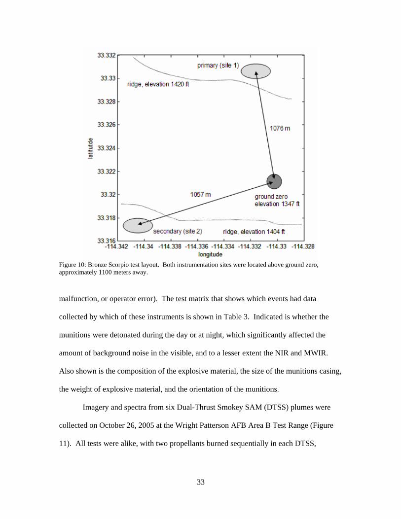
Figure 10: Bronze Scorpio test layout. Both instrumentation sites were located above ground zero, approximately 1100 meters away.

malfunction, or operator error). The test matrix that shows which events had data

collected by which of these instruments is shown in Table 3. Indicated is whether the

munitions were detonated during the day or at night, which significantly affected the

amount of background noise in the visible, and to a lesser extent the NIR and MWIR.

Also shown is the composition of the explosive material, the size of the munitions casing,

the weight of explosive material, and the orientation of the munitions.

Imagery and spectra from six Dual-Thrust Smokey SAM (DTSS) plumes were

collected on October 26, 2005 at the Wright Patterson AFB Area B Test Range (Figure

11). All tests were alike, with two propellants burned sequentially in each DTSS,

34

Table 3: Test matrix for Bronze Scorpio. Data collected and examined are denoted by a “Y”; data that have yet to be acquired by AFIT (not examined) are denoted by an “X”.

# Light Munitions Size Weight Orient. Phantom Indigo Irris Canon 1 day TNT 155mm 6.64 kg Erect Y Y X Y 2 day TNT 155mm 6.64 kg Erect Y X Y 3 day TNT 155mm 6.64 kg Erect Y Y X Y 4 day TNT 155mm 6.64 kg Erect Y X Y 5 day TNT 155mm 6.64 kg Erect Y Y X Y 6 day TNT 155mm 6.64 kg Prone Y X Y 7 day TNT 155mm 6.64 kg Prone Y Y X Y 8 day TNT 155mm 6.64 kg Prone Y X Y 9 day TNT 155mm 6.64 kg Prone Y Y X Y 10 day TNT 155mm 6.64 kg Prone Y Y X Y 11 day TNT 105mm 2.09 kg Erect Y X Y 12 day TNT 105mm 2.09 kg Erect Y Y X Y 13 day TNT 105mm 2.09 kg Erect Y X Y 14 day TNT 105mm 2.09 kg Erect Y Y X Y 15 day TNT 105mm 2.09 kg Erect Y X Y 16 day TNT 105mm 2.09 kg Prone Y Y X Y 17 day TNT 105mm 2.09 kg Prone Y X Y 18 day TNT 105mm 2.09 kg Prone Y Y X Y 19 day TNT 105mm 2.09 kg Prone Y Y X Y 20 day TNT 105mm 2.09 kg Prone Y X Y 21 day C-4 3x0.57 kg Y Y Y Y 22 night TNT 155mm 6.64 kg Erect Y Y X 23 night TNT 155mm 6.64 kg Erect Y Y Y X 24 night TNT 155mm 6.64 kg Erect Y Y X 25 night TNT 155mm 6.64 kg Erect Y Y X 26 night TNT 155mm 6.64 kg Erect Y Y Y X 27 night TNT 155mm 6.64 kg Prone Y Y Y X 28 night TNT 155mm 6.64 kg Prone Y Y X 29 night TNT 155mm 6.64 kg Prone Y Y Y X 30 night TNT 155mm 6.64 kg Prone Y Y X 31 night TNT 155mm 6.64 kg Prone Y Y X 32 night TNT 105mm 2.09 kg Erect Y Y X 33 night TNT 105mm 2.09 kg Erect Y Y Y X 34 night TNT 105mm 2.09 kg Erect Y Y X 35 night TNT 105mm 2.09 kg Erect Y Y Y X 36 night C-4 4.55 kg Y Y X 37 night TNT 105mm 2.09 kg Erect Y Y X 38 night TNT 105mm 2.09 kg Erect Y Y X 39 night TNT 105mm 2.09 kg Erect Y Y Y X 40 night TNT 105mm 2.09 kg Erect Y Y X 41 night TNT 105mm 2.09 kg Erect Y Y X 42 night TNT 105mm 2.09 kg Erect Y Y Y X 43 night C-4 4.55 kg Y Y X 44 night C-4 4.55 kg Y Y X

35

# Light Munitions Size Weight Orient. Phantom Indigo Irris Canon 45 night TNT 155mm 6.64 kg Erect Y Y X 46 day TNT 155mm 6.64 kg Erect Y Y Y X 47 day TNT 155mm 6.64 kg Erect Y Y Y Y 48 day C-4 4.55 kg Y Y Y 49 day TNT 155mm 6.64 kg Erect Y Y 50 day TNT 155mm 6.64 kg Erect Y Y Y 51 day TNT 155mm 6.64 kg Erect Y Y Y 52 day TNT 155mm 6.64 kg Erect Y Y Y Y 53 day C-4 4.55 kg Y Y Y Y 54 day Comp. B 155mm 6.64 kg Erect Y Y Y Y 55 day Comp. B 155mm 6.64 kg Erect Y Y 56 day Comp. B 155mm 6.64 kg Erect Y Y Y Y 57 day Comp. B 2x155mm 2x6.64 kg Erect Y Y Y Y 58 day Comp. B 155 mm 6.64 kg Erect Y Y Y 59 day Comp. B 2x155mm 2x6.64 kg Erect Y Y Y Y 60 day Comp. B 155mm 6.64 kg Erect Y Y Y 61 day Comp. B 2x155mm 2x6.64 kg Erect Y Y Y Y 62 day TNT 155mm 6.64 kg Erect Y Y 63 day TNT/C-4* 155mm/ 6.64/13.64 kg Y Y Y 64 day TNT/C-4* 155mm/ 6.64/13.64 kg Y Y 65 day C-4 13.64 kg Y Y Y

* munitions placed in a barrel

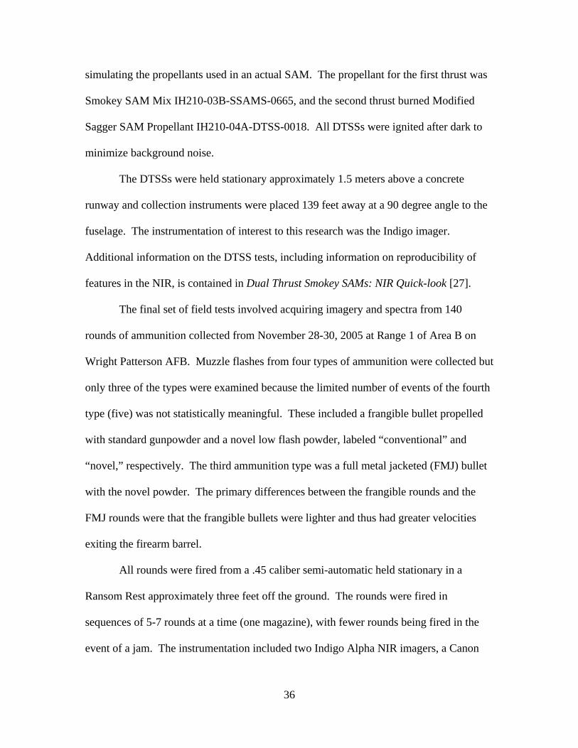
Figure 11: Dual Thrust Smokey SAM test setup at Wright Patterson AFB, Area B Test Range. The DTSS was fixed approximately 1.5 meters above a concrete runway.

36

simulating the propellants used in an actual SAM. The propellant for the first thrust was

Smokey SAM Mix IH210-03B-SSAMS-0665, and the second thrust burned Modified

Sagger SAM Propellant IH210-04A-DTSS-0018. All DTSSs were ignited after dark to

minimize background noise.

The DTSSs were held stationary approximately 1.5 meters above a concrete

runway and collection instruments were placed 139 feet away at a 90 degree angle to the

fuselage. The instrumentation of interest to this research was the Indigo imager.

Additional information on the DTSS tests, including information on reproducibility of

features in the NIR, is contained in Dual Thrust Smokey SAMs: NIR Quick-look [27].

The final set of field tests involved acquiring imagery and spectra from 140

rounds of ammunition collected from November 28-30, 2005 at Range 1 of Area B on

Wright Patterson AFB. Muzzle flashes from four types of ammunition were collected but

only three of the types were examined because the limited number of events of the fourth

type (five) was not statistically meaningful. These included a frangible bullet propelled

with standard gunpowder and a novel low flash powder, labeled “conventional” and

“novel,” respectively. The third ammunition type was a full metal jacketed (FMJ) bullet

with the novel powder. The primary differences between the frangible rounds and the

FMJ rounds were that the frangible bullets were lighter and thus had greater velocities

exiting the firearm barrel.

All rounds were fired from a .45 caliber semi-automatic held stationary in a

Ransom Rest approximately three feet off the ground. The rounds were fired in

sequences of 5-7 rounds at a time (one magazine), with fewer rounds being fired in the

event of a jam. The instrumentation included two Indigo Alpha NIR imagers, a Canon

37

RGB imager, a high speed Phantom RGB imager, an ABB Bomem MR-254 spectro-

radiometer, an ABB Bomem MR-154 spectro-radiometer, and an Acton visible grating

spectrometer, with the latter three not being discussed because they were not used in this

research.

Of importance to the current analysis was the Indigo imager located perpendicular

to the barrel at 181 cm. The test matrix indicating how many and what type of rounds

were fired in each sequence, as well as how many rounds were acquired with the Indigo

imager used, is shown in Table 4. Additional information on the Muzzle Flash tests and

the novel “flashless” powder can be found in Muzzle Flash Test: NIR Quick-look and

Conventional and Q30 Flashless Gunpowder Preliminary Test Report [28][29].

Figure 12: Muzzle Flash Test setup geometry.

38

Table 4: Test matrix for Muzzle Flash Tests indicating ammunition type, number of rounds fired, and number of rounds acquired with the Indigo imager.

Sequence Ammunition # rounds # acquired fraction 001 conventional 7 4 0.571 002 conventional 6 3 0.500 003 conventional 4 2 0.500 004 conventional 7 2 0.286 005 novel 7 1 0.143 006 novel 6 4 0.667 007 novel 7 3 0.429 008 novel 7 1 0.143 009 conventional 1 1 1.000 010 conventional 7 4 0.571 011 conventional 1 1 1.000 012 conventional 7 4 0.571 013 conventional 5 1 0.200 014 conventional 2 0 0.000 015 conventional 1 0 0.000 016 conventional 6 1 0.167 017 conventional 5 0 0.000 018 novel 3 2 0.667 019 novel 4 1 0.250 020 novel 7 1 0.143 021 novel 7 5 0.714 022 novel 2 1 0.500 023 novel FMJ 1 1 1.000 024 novel FMJ 6 4 0.667 025 novel FMJ 6 3 0.500 026 novel FMJ 6 3 0.500 027 novel FMJ 6 2 0.333 028 Wolf 1 1 1.000 029 Wolf 5 1 0.200 Total 140 57 0.407

Data Extraction

Analysis of the afterburn fireballs, DTSS plumes, and muzzle flashes was not

conducted on the raw imagery files acquired by each instrument. Rather, the data were

input into Matlab where more sophisticated data processing could be used. For the

Indigo and Irris imagers, this was accomplished with Matlab scripts (written by Tom

39

Fitzgerald of ATK Mission Research) that read the raw data directly from the

instrument’s imagery file and saved them in a Matlab structure. For every frame of

imagery, the Matlab structure contained a matrix representing the digital numbers (DNs)

of each pixel. Since both imagers are 12-bit, these DNs ranged between zero (no signal)

and 4095 (saturation).

Importing the Phantom imagery into Matlab was more complicated because the

imagery files use a proprietary file structure. Without knowing how the files were

encoded, a reader could not be developed. Instead, imagery from the Phantom camera

was converted to an uncompressed, 24-bit AVI movie. These were read into Matlab

structures using built-in Matlab functions. The structures were similar to that of the IR

imagers, with the difference being that the Phantom structures contained a matrix of 8-bit

DN values for each of the RGB bands for each frame. This preserved the quality of the

data, but due to the extremely large AVI file sizes, processing time was extensive.

The Phantom camera provided imagery of the shockwave in addition to the

fireball. The shocks were visible, albeit faintly, due to the change in index of refraction

they caused as they passed through the atmosphere (see Figure 13 – the shockwave is

visible in the video but very difficult to distinguish in a static image without image

processing). Since viewing the shock depends on viewing the disturbance it causes to

light passing through it (from the landscape in the background), the shock could only be

seen for events that occurred during the day. Additionally, due to the variations in the

landscape, automated processing of the shockwave’s position was not attempted. Instead,

the position of the shock relative to the point of detonation was measured manually in

steps of 5-10 ms from the time it was first visible until the shock exited the field of view;

40

Figure 13: Static image of a Bronze Scorpio detonation with its shockwave (left) and the same image after image processing (right). The index change due to the shockwave is difficult to see in the original image, but with background subtraction and contrast adjustment, it can be seen as a nearly spherical shell propagating away from the detonation.

this amounted to six to ten data points. A late-time data point was obtained using the

Canon video to determine the time of detonation and then listening for the boom as the

shockwave reached the camera on the audio track.

There was an uncertainty of approximately 10 pixels in the measurement of the

shockwave’s position. This was due to the thickness of the shockwave and its faintness,

both of which made it difficult to distinguish where its position could consistently be

measured. Taking the IFOV of the Phantom camera into account, this translates into

approximately half of a meter. The uncertainty in the late-time measurement of the shock

position was approximately 0.3 seconds. This is an uncertainty of approximately ten

percent, but it gave a rough approximation of the velocity of the shockwave at the

measurement site (and thus the extent to which the shockwave had transformed to an

acoustic wave).

Ideally, the shockwave would be spherically symmetric and measurements of the

shockwave shockwave

41

shock position could be taken in any direction. In reality, the shock appeared elliptical at

early times (although it approached spherical rather quickly) and so for consistency, the

position of the shock was measured in the vertical direction. The position and time

values were stored in an Excel spreadsheet that was accessible to both TableCurve 2D for

curve fitting and Matlab for analysis.

Data Processing

In general, the events being observed occupied only a fraction of the field of view

of the instrument and an even smaller fraction of the total number of frames recorded.

This inflated file sizes with useless data and made processing go much more slowly. To

more efficiently handle data, the Matlab structures were truncated by eliminating all but a

handful of background frames. Additionally, the event matrices were cropped on all

sides to slightly larger than the event dimensions. This can be seen for the NIR imagery

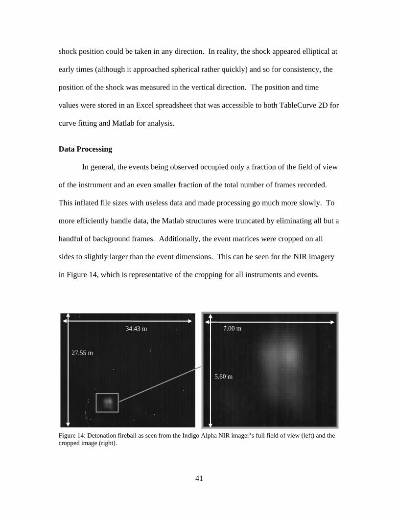
in Figure 14, which is representative of the cropping for all instruments and events.

Figure 14: Detonation fireball as seen from the Indigo Alpha NIR imager’s full field of view (left) and the cropped image (right).

34.43 m

27.55 m

7.00 m

5.60 m

42

The above processing did not alter the data from their raw format. In order to

perform calculations for the fireballs in the Phantom’s blue band, however, hot pixels –

pixels with a DN above some threshold value – that were not associated with the fireball

needed to be removed. This was because calculations of the fireball area were dependent

on hot pixels, and non-fireball hot pixels would skew the result (the exact criteria for a

pixel being hot are discussed in the Area Profiles section). These were pixels that viewed

the smoke and debris cloud near to the ground and were saturated by reflected or emitted

light in the blue band only (see Figure 15). Removing them was accomplished by

applying a mask to each frame of the blue imagery so that only the region around the

fireball remained. The mask was computed by identifying the hot pixels in the red band

and defining a rectangular region with a ten pixel buffer to each side. Everything in the

blue matrix outside of this mask was set to a digital number of zero.

Figure 15: Detonation fireball as viewed by the Phantom camera in the red (upper left), green (upper right), and blue (lower left) bands. Due to the brightness of the smoke and debris in the blue band, the blue image was masked (lower right) so that only hot fireball pixels would be seen. The mask was based on hot pixels in the red band, with a ten pixel buffer on each side.

red green

blue

22.20 m

17.75 m

masked blue

43

Area Profiles

The simplest features of the fireball to extract from imagery were those relating to

the size and duration of the fireball (missile plumes and muzzle flashes had many of the

same features and, although not always explicitly mentioned, these types of combustion

events are assumed to be included in descriptions of fireball feature extraction). To

examine the fireballs’ characteristics quantitatively, metrics had to be established that

gauged the fireball’s size and duration. The metrics used were taken from the histograms

of the imagery as a function of time, as in Figure 16. In these temporal histograms, the

numbers of pixels, N, as functions of digital number are plotted for each frame of

imagery for a munition detonation in the MWIR (left) and a DTSS plume in the NIR

(right). While the distribution of DNs was band dependent and varied for event type, the

common characteristics included a spike in pixel number at low DNs corresponding to

background, low pixel numbers in the mid DNs before and during the combustion event,

and a smaller spike in the high DNs from pixels illuminated by combustion emissions.

Because of the bimodal distribution, the histograms provided an opportune way to

determine fireball size – the spike in high DNs corresponds to fireball illuminated pixels.

The size of the fireball (for each frame of the image) was calculated by summing over the

number of pixels at each digital number in the histogram, Ni, that were above some

threshold and then multiplying by the area viewed per pixel (Equation 25). From

geometry, the area viewed per pixel, Apx, as a function of the IFOV of the instrument, θpx,

and the distance from the event, d, is given in Equation 26.

This metric provides an area profile as a function of frame (but was converted to a

function of time by dividing by the instrument’s frame-rate) and is referred to as the

44

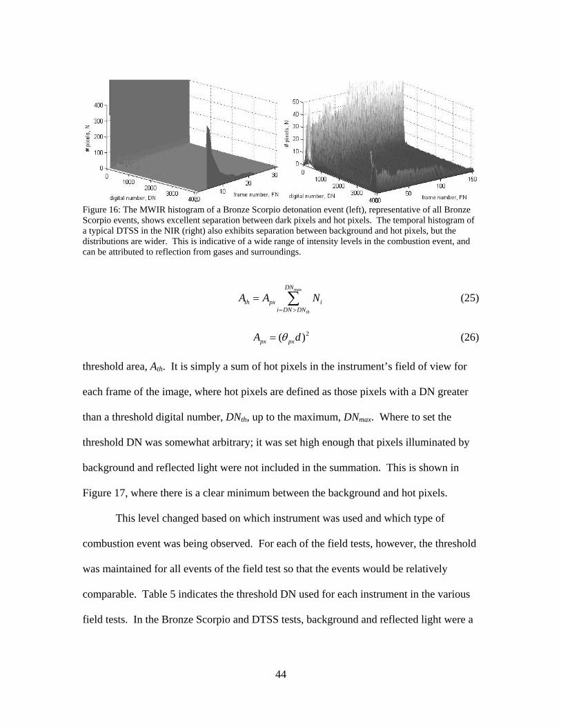
Figure 16: The MWIR histogram of a Bronze Scorpio detonation event (left), representative of all Bronze Scorpio events, shows excellent separation between dark pixels and hot pixels. The temporal histogram of a typical DTSS in the NIR (right) also exhibits separation between background and hot pixels, but the distributions are wider. This is indicative of a wide range of intensity levels in the combustion event, and can be attributed to reflection from gases and surroundings.

max

th

DN

th px ii DN DN

A A N= >

= ∑ (25)

2( )px pxA dθ= (26)

threshold area, Ath. It is simply a sum of hot pixels in the instrument’s field of view for

each frame of the image, where hot pixels are defined as those pixels with a DN greater

than a threshold digital number, DNth, up to the maximum, DNmax. Where to set the

threshold DN was somewhat arbitrary; it was set high enough that pixels illuminated by

background and reflected light were not included in the summation. This is shown in

Figure 17, where there is a clear minimum between the background and hot pixels.

This level changed based on which instrument was used and which type of

combustion event was being observed. For each of the field tests, however, the threshold

was maintained for all events of the field test so that the events would be relatively

comparable. Table 5 indicates the threshold DN used for each instrument in the various

field tests. In the Bronze Scorpio and DTSS tests, background and reflected light were a

45

Figure 17: The histogram as a function of time shows a minima near DN 3000. Setting the threshold here (dashed line) assumes that all DNs above this level are due to combustion emissions and that all DNs below this are due to background or reflected light.

concern, so the threshold was set where there appeared to be a minimum in the

histogram. In the Muzzle Flash test, however, all events occurred in the dark with a

black background, so background and reflected light were not an issue. Because of this,

all DNs above the background (calculated as the DNs above which the number of pixels,

N, dropped below 1% of the maximum of the background spike) were considered muzzle

flash areas. This level was variable, but was typically around DN 600 and was most

likely due to light reflected from gases ejected from the muzzle. The area of the brightest

part of the plume (the part thought to be emitting) was based on a threshold of DN 3800.

Histograms, thresholds, and imagery of a single frame of each combustion event are

shown in Figure 18.

46

Table 5: Threshold DN for each instrument used in the three field tests. In the Muzzle Flash test, there were two thresholds. The first measured everything above background and was variable for each event. It was set where the background DN spike drop below 1% of its maximum value, typically around DN 600. The second threshold quantized only the DNs of the bright flash and was fixed.

Instrument DNmax Bronze Scorpio DNth DTSS DNth Muzzle Flash DNth Phantom 255 254 Indigo 4095 3276 3000 600* / 3800 Irris 4095 3276

* typical value

Figure 18: NIR histograms (left) for the corresponding frame of the combustion even (right). From top to bottom, the events are a muzzle flash, DTSS plume, and afterburn fireball. The gray shading in the histogram corresponds to the average background, and the black shading corresponds to the DNs of the event. The threshold levels are indicated with a dashed line.

As can be seen in the histograms, the value at which the threshold DN should be

set was not always obvious – there was not always a clear minimum in the separation of

background/reflected light and emitted light. Moving the threshold DN up or down,

however, did not affect the threshold area profile as a function of time. If it had,

determination of the threshold level would have been much more important because it

47

would have indicated new features were being included or discarded. Rather, changing

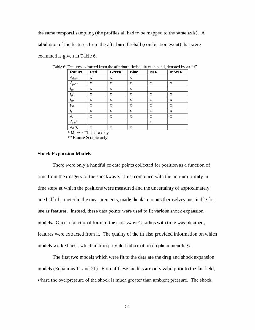
the threshold merely changed the magnitude of the area profile, as is seen in Figure 19.

Maintaining a consistent threshold level for all events in the test was more important to

feature comparison than determining the absolute level (if one exists) at which DNs

shifted from background and reflection to combustion emissions.

The threshold area was not the only area profile used to examine the size of the

afterburn fireball. Four other methods were used to characterize the area profile as a

function of time, all of which (erroneously) approximate the fireball as spherical. Two of

these included finding the mean location of the hot pixels at the time of detonation, thus

Figure 19: The MWIR area profile of Bronze Scorpio event 26 is relatively independent of the threshold level. Changing the threshold from 20% of the dynamic range through 90% changes only the magnitude of the area, but not its shape as a function of time. The scaling factors, S, for each threshold level, th, are indicated below the plots.

48

locating the detonation origin. The distance to the maximum hot pixel from the origin

defined a radius, that when squared and multiplied by π, gave an area profile termed the

maximum static area, 0maxA . The maximum dynamic area, maxA , was calculated in the

same manner as 0maxA except that the origin was calculated for each frame (under the

assumption that the fireball translated as it evolved). Both of these metrics overestimated

fireball size by assuming that cool pixels (those below threshold) closer to the origin than

the maximum radius were fireball that was obscured by dirt, smoke, and other debris.

The remaining two area metrics also used the static and dynamic origin. In these,

however, the standard deviation of the distance between the origin and all hot pixels in

the image was found. This defined a statistical radius that assumed the obscured fireball

was distributed normally and that the area determined by taking three times this radius

(three standard deviations) encompassed 99% of the fireball. These area profiles were

termed three sigma static area, 03A σ , and three sigma dynamic area, 3A σ .

The five area profiles of a munitions detonation are shown in Figure 20 for

reference. Because of the range of magnitudes involved – less than ten to greater than

one hundred square meters – the log of the areas are plotted as a function of time. It is

clear that each profile is different, and thus each will have different features that can be

extracted from it. In this research, however, time was limited and features were only

extracted from the threshold area profile. The others are mentioned because they show

potential for use in classification and phenomenology in future study. In the remainder of

this paper, the terms area and area profile will refer to threshold area and threshold area

profiles.

49

Figure 20: The five area profiles are plotted for a Bronze Scorpio event in the red band. Threshold area (solid dark line) is several orders of magnitude below the maximum static (dotted dark like) and maximum dynamic (dotted gray line) areas. The three sigma static profile (dashed dark line) predicts the largest area, but the three sigma dynamic area (dashed gray line) has a much lower magnitude.

Combustion Features

By examining the area profile for a typical Bronze Scorpio detonation (Figure

21), several features are apparent. These include the sharp spike in the area profile due to

the initial flash at detonation, detA , the peak area of the afterburn fireball (or more

generically, the peak area of the combustion event), pkA , and the times after detonation

that these peaks occur, dett and pkt . Three additional features relating to the duration of

the fireball are the time at which its area falls below 50% and 10% of pkA , denoted by t50

and t10, and the time at which the area falls within three standard deviations of the

average noise level, tn. The total area under the curve, At, is found by integrating the area

profile with respect to time.

With the exception of the detonation peak features, these features were valid for

all of the imagers (the detonation features could not be extracted in the IR because the

Ath

A3σ

03A σ

0maxA

Amax

50

instruments were too slow to resolve the initial spike). These features were also extracted

from the DTSS plume, excluding the detonation spike (because there was no detonation

flash in the missile plume). The muzzle flashes, however, were very short lived and

occupied only a single frame of imagery. Because of this, there was no area profile, but

rather a single (peak) area – the area of the muzzle flash, pkA . The goal of these tests was

to determine the visibility of the flash; thus pkA includes everything above background,

both from reflection and emission. A second feature that was extracted from the muzzle

flash is the area of strong emission characterized by DNs near saturation. This is the

flash (or saturation) area, Asat, and as mentioned previously, includes DNs above 3800.

Finally, because of the extremely high temporal resolution of the Phantom

camera, the area profiles in the red, green, and blue were used as features. This was

accomplished by interpolating the area profiles for each event onto a uniform time axis

ranging from zero (detonation) to 200 milliseconds (well after the fireball has decayed) in

steps of 0.1 milliseconds. This interpolation was necessary for comparing the time

dependent features, since a point by point comparison required all of the profiles to have

Figure 21: Threshold area profile as a function time for a Bronze Scorpio detonation in the red band. The features that may be extracted from the profile are indicated.

tA

det det( , )t A ( , )pk pkt A

10t

50t

nt

51

the same temporal sampling (the profiles all had to be mapped to the same axis). A

tabulation of the features from the afterburn fireball (combustion event) that were

examined is given in Table 6.

Table 6: Features extracted from the afterburn fireball in each band, denoted by an “x”. feature Red Green Blue NIR MWIR Adet** x x x Apk** x x x x x tdet x x x tpk x x x x x t50 x x x x x t10 x x x x x tn x x x x x At x x x x x Asat* x Ath(t) x x x

* Muzzle Flash test only ** Bronze Scorpio only

Shock Expansion Models

There were only a handful of data points collected for position as a function of

time from the imagery of the shockwave. This, combined with the non-uniformity in

time steps at which the positions were measured and the uncertainty of approximately

one half of a meter in the measurements, made the data points themselves unsuitable for

use as features. Instead, these data points were used to fit various shock expansion

models. Once a functional form of the shockwave’s radius with time was obtained,

features were extracted from it. The quality of the fit also provided information on which

models worked best, which in turn provided information on phenomenology.

The first two models which were fit to the data are the drag and shock expansion

models (Equations 11 and 21). Both of these models are only valid prior to the far-field,

where the overpressure of the shock is much greater than ambient pressure. The shock

52

model is also not valid in the near-field, where the mass of the explosive is not negligible.

The region where both models are valid is quantized by Equation 17. Inserting values of

ED, and m0 from the properties of TNT and Composition B, and assuming values of 1.4,

1.2 kg/m3, and 1 atm for γ, ρ0, and p0, the limiting values of the mid-range for the

munitions studied in the Bronze Scorpio tests were calculated and are shown in Table 7.

The values of detonation energy used for Composition B were not found in the

literature and had to be approximated. By assuming the energies released by the TNT

and the RDX in the initial detonation are independent of each other, the heat of

detonation of Composition B can be assumed to scale in proportion to the mixture ratios

(Equation 27). This estimates the energy released in the detonation of Composition B to

be 5573 kJ/kg, which when multiplied by the mass of Composition B, is the value that

was used for the energy released in the detonation, ED, in the above table.

0.39 0.6 0.39(4563) 0.6(6322) 5573CompB TNT RDX

D D DH H H∆ = ∆ + ∆ = + = (27)

Because the position of the shock was examined at distances extending well into

the far-field (both from data points taken from the Phantom imagery and the late-time

Table 7: Material properties are shown for each munition in the Bronze Scorpio tests. These, along with the assumed atmospheric properties (also shown), allowed the near- and far-field radii to be calculated.

property 155mm TNT 105mm TNT 155mm Comp. B 2x155mm Comp. B ED (J) 30298320 9536670 37004720 74009440 p0 (Pa) 101325 101325 101325 101325 ρ0 (kg/m3) 1.2 1.2 1.2 1.2 m0 (kg) 6.64 2.09 6.64 13.28 γ 1.4 1.4 1.4 1.4 ξ0 1.165 1.165 1.165 1.165 near-field R (m) 1.097 0.746 1.097 1.382 far-field R (m) 2.426 1.650 2.593 3.267

53

point from the Canon audio), it was necessary to also use models which could take the

late-time behavior of the shockwave into account. As stated previously, as the shock’s

overpressure and velocity decrease, it gradually transitions from a shockwave to an

acoustic wave traveling at the speed of sound, c0. A modification of the explosive model

that approximates the mid-field and far-field behavior is the linear combination of the

mid-field and far-field solutions (Equations 11 and 18). While this functional form

causes deviation from the true model, it captures the basic growth of the fireball in both

the mid-field and far-field. The t2/5 causes the mid-field term to dominate at early times

but become negligible later, whereas the t makes the far-field term small at early times

but more important at later times. The form shown in Equation 28 approximates the

extent of the shockwave as a function of time in both regions.

1

52

0 00

( ) DE tR t c tξρ

⎛ ⎞⋅= +⎜ ⎟

⎝ ⎠ (28)

The basic drag model also fails to capture the far-field approach to the speed of

sound and instead has the shock approaching a zero final velocity. By modifying the

equation of motion governing the shock’s behavior, however, a functional form with a

final velocity of c0 can be found. This is shown in Equation 29 where the deceleration is

set proportional to the difference between shock’s velocity and the speed of sound; when

the shock’s velocity reaches the speed of sound it stops decelerating. Solving for the

shock velocity as a function of time (Equation 30) and then integrating with respect to

time (and imposing the boundary condition of zero radius at detonation) yields Equation

31. This modified drag model captures the viscous deceleration of the drag model with

the recognized asymptotic behavior of shockwaves at late times.

54

( )0dD D cdt

β= − − (29)

0 0( ) tD t D e cβ−= + (30)

( ) ( )00 max 0( ) 1 1t tDR t e c t R e c tβ β

β− −= − + = − + (31)

Shock Expansion Fits

The four models given above were used to generate six fit functions of the time

dependence of the shock’s position, R(t). All physical quantities that could be combined,

such as 1

50 0( / )DEξ ρ , were combined into single fit parameters a, b, or c. These fit

functions are shown in Equations 32 through 37. The first two are the explosive and drag

models as functions of only two fit parameters, a and b. The second pair of fit functions

consists of the modified explosive and modified drag models as functions of three fit

parameters: a, b, and c. In these functions, the final velocity of the shock (the speed of

sound in air, represented by the c fit parameter) is left variable. The purpose of this was

to improve the quality of the fit as well as to verify that the shock velocity did indeed

approach the speed of sound – if fit parameter c took on values near c0 as a result of the

best fit, it would be evidence that the shockwave did indeed transition to an acoustic

wave. The final two equations are the modified explosive and drag models with the

speed of sound fixed. This was to ensure that the modified shock and drag models did

not fit the data better than their unmodified counterparts merely because they contained

an additional fit parameter. The value used for c0 was 350 m/s, which corresponds to a

temperature of 30.33°C. This was warm for November in Yuma, AZ; the actual range of

55

temperatures was 11°C to 26°C which corresponds to values of c0 ranging from 338.11

m/s to 347.26 m/s [30][31].

( ) bR t a t= ⋅ (32)

( ) (1 )b tR t a e− ⋅= ⋅ − (33)

( ) bR t a t c t= ⋅ + ⋅ (34)

( ) (1 )b tR t a e c t− ⋅= ⋅ − + ⋅ (35)

0( ) bR t a t c t= ⋅ + ⋅ (36)

0( ) (1 )b tR t a e c t− ⋅= ⋅ − + ⋅ (37)

The position as a function of time, excluding the late-time data point from the

Canon camera, was imported into TableCurve 2D (the late-time data point was used to

evaluate the quality of the fit at late times). TableCurve 2D uses least-squares fitting

routines to fit the input data to user-defined functions. After fitting the functions to the

data for each event, the fit parameters, their uncertainties, and the correlation coefficient

between the fit and the data were exported into Matlab for feature extraction.

Shockwave Features

Because the only shockwave information that was used was the position at

various times, all of the extracted features were directly or indirectly related to its

expansion. Because of how the features were compared (discussed in the Feature

Analysis section), however, it was useful to transform the position fits to other physical

quantities using known relations.

The first of these transformations was simply a determination of the velocity of

56

the shockwave as a function of time, accomplished by taking the derivative of the fit

function with respect to time. This was put in terms of the Mach number, M. This is

shown in Equation 38, where, for consistency the temperature was fixed at 30.33 °C and

c0 was 350 m/s.

0 0

( ) 1( ) D t dRM tc c dt

= = (38)

With the Mach number known as a function of time, the pressure of the

shockwave was found using Equation 7. Using the empirical relationship between

overpressure and scaled distance, the shockwave’s pressure could be related back to an

initial release of energy in the detonation, ED. An analytic approximation was

determined, however, so that all calculations could remain analytic. The least-squares fit

of the base 10 log of the scaled distance to the base 10 log of the pressure was found,

with the base 10 logs used to more equally weight the data (because the data spanned

several orders of magnitude). The approximation is shown in Equation 39 and had

excellent correlation for the weighted data ( 2 0.988r = ) and agreement within 30% for

the unweighted data.

03/51

psp

= (39)

If the detonation were truly ideal, all of the energy would have been released

instantaneously and ED would have been constant. Since real munitions detonations are

not ideal, however, the apparent energy released became functionally dependent on the

time at which the shockwave was examined. Substituting Equation 39 into Equation 10

provides this relationship, which is shown in Equation 40.

57

3

9/51

0

( )( ) ( ) TNTD D

R tE t p t Hp

⎛ ⎞= ∆⎜ ⎟⎝ ⎠

(40)

All of the above physical quantities, R(t), M(t), p1(t), and ED(t), as calculated from

all six fit functions, were used as features of the shockwave. Since they all evolve with

time, the function for each physical quantity was evaluated for all times between 0 and

200 milliseconds in steps of 0.1 milliseconds. This led to an enormous number of

features that for small separations in time were very closely related. Because of this, only

one time step of each feature was used (in comparisons to other features) – but all were

evaluated to determine which time yielded the best results.

Another feature of the shockwave (for each fit function) was the efficiency of the

detonation, f. This was calculated as a ratio of the detonation energy that was derived

from experimental data to the theoretically determined energy of detonation, as shown in

Equation 41. It was used as a feature to determine if there was a correlation between the

fractions of energy released in the detonation to the variability in other extracted features.

Like the other time-dependent shock features, it was sampled in 0.1 ms increments from

0 to 200 ms, but only one value was used per comparison.

0

( )( ) D

D

E tf tH m

=∆

(41)

Finally, the fit parameters a, b, and c for each of the fit functions were used as

features of the shockwave. This brought the number of shockwave related features to a

total of forty-four (five time dependent features for each of the six fit functions giving a

total of thirty physical features, plus an additional fourteen fit parameters from the fit

functions themselves).

58

Feature Analysis

The primary questions to be answered in this research (which features of the

shockwave, fireball, and explosive munitions are reproducible, provide distinguishability,

and are correlated with other features?) guided this research in the final phase of data

analysis. The first step in answering these questions was to specify how the combustion

events were to be categorized. There were five different munitions used in the Bronze

Scorpio field tests, detonated in nine total arrangements. Each of the unique

arrangements was referred to as a type. Combinations of arrangements were referred to

as a group, and categories of combustion events were referred to as a class. For example,

155 mm TNT was a group, but when specifying an orientation, such as 155 mm TNT

erect, the unique arrangement was a type. DTSS plumes and muzzle flashes (along with

detonations) were classes of combustion events. If all tests were included, the number of

types of combustion events was brought up to fourteen. These types and their use in

analysis are shown in Table 8.

Grouping these types together was necessary for two reasons. The primary need

was the sparsity of the data set. There were a limited number of events of each type and

an even fewer number of events acquired by all of the instruments for each type. If only

a single type was examined, there were approximately half a dozen or fewer acquired

events. By grouping the types, such as all TNT (types 1-4), the number of data points for

any given feature increased and became more statistically meaningful. The second

reason for grouping the types was to determine which features were unique to the group

and which features were unique to the type. Some features were independent of weight

but depended very strongly on explosive material, indicating they were features of the

59

explosive material group. On the other hand, a feature that did depend on the weight was

a type feature. Grouping showed which features scaled with which properties of the

group and type.

The groups that were examined are given in Table 9. The five munitions were

examined individually, as well as in combination with other munitions of the same

weight or explosive material. These small groups of one or two types provided

information on reproducibility of features and the ability of these features to differentiate

between other types or groups. Many of these did not contain enough data points to be

Table 8: Types used in analysis. “Y” indicates use as a stand-alone type, “X” indicated that the type was not analyzed separately but was used in groups with other types, and “N” indicates no analysis was performed on the type.

Type # Field Test Arrangement Used in Analysis 1 Bronze Scorpio 155mm TNT erect Y 2 Bronze Scorpio 155mm TNT prone Y 3 Bronze Scorpio 105mm TNT erect Y 4 Bronze Scorpio 105mm TNT prone Y 5 Bronze Scorpio 3x1.25# C-4 X 6 Bronze Scorpio 10# C-4 X 7 Bronze Scorpio 155mm Composition B erect Y 8 Bronze Scorpio 2x155mm Composition B erect Y 9 Bronze Scorpio 155mm TNT / 30# C-4 / barrel X 10 DTSS Dual Thrust Smokey SAM Y 11 Muzzle Flash Conventional Y 12 Muzzle Flash Novel Y 13 Muzzle Flash Novel FMJ Y 14 Muzzle Flash Wolf N

Table 9: Grouping of types for reproducibility, distinguishability, and correlation analysis Group # 1 2 3 4 5 6 7 8 Types 1 2 3 4 1,2 3,4 1-4 8

Group # 9 10 11 12 13 14 15 16 Types 7,8 1-4,7,8 1-9 10 11 12 13 11-13

60

meaningful, but it was still useful to see if they produced any results that showed promise

for further investigation. The broader groups, i.e. all explosive munitions (types 1-9),

weren’t particularly useful for reproducibility or distinguishability, but gave a large range

of values in the feature sets to determine correlations.

The next step was to determine which features are reproducible. This was

performed by calculating the coefficient of variation. Since the CV is a statistical metric

based on the mean and standard deviation of the feature set, differing which types of

munitions were included in the set (group) changed its value. The CV was calculated in

Matlab for all extracted features in all bands for all groups. For features with time

dependence, the CV was calculated for each time step and the mean value used as a

characterization of the feature’s reproducibility. This generated an extensive list of

values that were sorted from best to worst (lowest CV to highest) for examination.

The Fisher Ratio was then determined by comparing two groups at a time to

determine distinguishability. Instead of using all groups in these comparisons, the groups

containing only a single munitions type were excluded. This was guided by the low

number of data points for each feature in single type groups. While this was acceptable

for calculating CV, comparisons of two groups where one is not statistically significant

would be meaningless for distinguishability. There were three sets of comparisons. The

first was a comparison of each class of combustion events against the others – this

demonstrated the ability to distinguish very dissimilar events and provided a baseline for

how well distinguishability using the FR performed. The second comparison used only

events from the Muzzle Flash test because these types contained features that are

relatively simple and reproducible within types. The more complex problem of

61

distinguishing groups of munitions detonations based on extracted features was also

examined. The groups that were compared are shown in Table 10. As with the CV, these

comparisons generated an extensive list of FR values that were sorted from best to worst

(highest to lowest).

Finally, the correlation between shockwave, fireball, and munitions features in the

Bronze Scorpio data set was evaluated based on their coefficient of determination, r2. In

these comparisons, the munitions features used were the mass, m0; energy released in the

detonation, ED; energy released in the afterburn fireball due to combustion, EA; heat of

detonation, DH∆ ; and the specific energy released in the afterburn fireball, AH∆ . The

time dependent features of the shockwave and fireball were compared at all time steps

and the one with the highest r2 was used as the feature. Since a wide range of feature

values were necessary to compute correlation, the groups were all TNT (group 7), all

TNT and Composition B (group 10), and all munitions (group 11).

The form of the correlation coefficient used here (Equation 24) determines the

linear correlation between two sets of data. A more general form could have been used if

other functional forms relating the two features were tested (such as exponential, inverse

power, etc.) but in this research, only power laws were tested (with one exception,

discussed in the Analysis and Results: Efficiency section). This was accomplished by

Table 10: The groups to be compared using the Fisher Ration are shown for each set of comparisons. These include comparing groups of all combustion events, groups of muzzle flashes only, and groups of munitions detonations only.

Field Tests Groups Types All 11,12,16 [1-9] [10] [11-13] Muzzle Flash 13-15 [11] [12] [13] Bronze Scorpio 5,6,7,9 [1,2] [3,4] [1-4] [7,8]

62

taking the square-root and cube-root of each of the fireball features and determining the

linear correlation of these features with the shockwave and munitions features. This

effectively determined whether the correlation with the fireball feature was best with a

linear, quadratic, or cubic power of the shockwave and munitions features. This is also

why all of the position-dependent shockwave features were used; even though the

pressure, Mach number, and apparent energy released all depended on measurements of

the shock’s position as a function of time, they are not related in a linear fashion. Thus,

when determining linear correlation, different forms of the same basic information

proved to be more useful. Because of the large number of coefficients of determination,

the values were sorted, and those features that were highly correlated were examined.

Summary

Detonations of explosive munitions are anything but simple phenomena.

Understanding them requires studying their behavior and trying to draw physically

meaningful conclusions. This was attempted here, with the results of the process –

experimentally observing fireballs and shockwaves in several bands of imagery,

determining profiles of the fireball area and models of the shockwave’s characteristics,

extracting features from the fireball area and shockwave properties, and assessing these

features for reproducibility, distinguishability, and correlation – providing a number of

findings. The next step was to examine these findings to try to extract the

aforementioned conclusions.

63

IV. Analysis and Results

Chapter Overview

This chapter attempts to answer the questions first posed in this research: which

features of the shockwave and afterburn fireball are reproducible and provide

distinguishability? Which of these features are correlated to characteristics of the

explosive munitions? And which of the features of the shockwave are correlated to

features of fireball?

Since reproducibility of features is dependent on only a single feature in a single

group of munitions, it was the simplest metric to examine and is the first one looked at

here. Next, the distinguishability of features was examined between different groups of

munitions. Those features with the highest reproducibility are best suited for recognizing

munitions types because they identify a consistent signature of an explosive munitions

group. These were not always the best features for classification, however, because some

features with low reproducibility still provided a high degree of classification, and vice

versa. Those features with promise for classification are presented.

Finally, the correlation of features extracted from the shockwave, fireball, and

munitions was examined. Those features that had the highest coefficients of

determination were used to find scaling laws for to all detonations, detonations of

explosives containing TNT, and pure TNT explosives. Also investigated were those

features that had low reproducibility to determine if variability in one feature was

correlated to variability in the other feature. A number of specific feature correlations

were examined and are discussed throughout the analysis.

64

Reproducibility of Area Profiles

Before examining which specific features are the most reproducible, looking at

the reproducibility of the area profiles as a function of time is instructive. Figure 22

shows the area profiles for the six individual erect 155mm TNT detonations (thin lines),

along with the mean profile (thick line) and the standard deviation (shaded region) of the

set; the plots shown are for the red band, but the green and blue bands show very similar

profiles. It is clear that even for events of the same weight, composition, and orientation

there is a great deal of variability in the fireball size as a function of time – the peak

fireball areas differ in both magnitude and time of occurrence, and the duration of the

fireball varies by a factor of two. The most reproducible aspects of the detonation appear

to occur at very early times (less than 10 milliseconds) and include the time and peak area

of the detonation.

If all TNT (155mm erect, 155mm prone, 105mm erect, and 105mm prone)

detonations are grouped together, the variability of the area profiles does not appreciably

Figure 22: The area profiles for all erect 155mm TNT detonations are shown (thin line) with their mean (thick line) and standard deviation (shaded region) in the upper plot. The CV as a function of time for the area profiles is shown on bottom. The mean CV value for the six events of this type’s feature is 1.22.

65

increase. This is evidenced in Figure 23 where the area profiles for all thirteen TNT

events are plotted, again from the red band. The magnitude of the mean profile decreases

for the afterburn fireball, but its shape remains nearly the same. The individual

detonation profiles show that there is also as much variation in the afterburn area, time to

afterburn peak, and duration as there was in the erect 155mm TNT. The conclusion that

can be inferred is that the variability in the area profiles of a single type is nearly the

same as it is for a group of munitions of the same composition, i.e. reproducibility is not

affected by weight or orientation. The average CV before the fireballs begin to decay

(prior to ~40 milliseconds, on average) is approximately one, indicating that the

variability in the area profile is of the same magnitude as the area itself.

The other explosives examined in this research were munitions containing

Composition B. The red band area profiles for all Composition B detonation events are

shown in Figure 24 (note that the timescale is different than for the TNT profiles). These

detonations have a shape that is very reproducible – a sharp spike in area at detonation

Figure 23: The area profiles for all TNT detonations are shown (thin line) with their mean (thick line) and standard deviation (shaded region) in the upper plot. The CV as a function of time for the area profiles is shown on bottom. The mean CV value for the thirteen events of this type’s feature is 1.6.

66

and then a very small area in the afterburn. The reproducibility of the magnitudes and

time to peak of the areas, however, is quite poor and has an average CV of 1.58 (possibly

due to obscuration, in which case a scaling factor accounting for this may improve

reproducibility). Without correction, however, the Composition B detonations showed as

much variability as the TNT detonations, indicating that the variability in observed area

profiles was not a function of explosive composition in the Bronze Scorpio field tests.

Finally, although the result is easily anticipated, plotting the area profiles of all

TNT and Composition B detonations shows greater variability for the combined group

than for either single composition group alone. This is seen in Figure 25 where the

average CV value is 1.98. The least reproducible features are the area, time to peak, and

duration of the afterburn fireball. Although the variability of the two groups of

compositions is approximately the same, the reproducibility of the area profiles decreases

when the two groups are combined into a single group. This is indicative that there are

features in the area profile that show some distinguishability for the different explosive

Figure 24: The area profiles for all Composition B detonations are shown (thin line) with their mean (thick line) and standard deviation (shaded region) in the upper plot. The CV as a function of time for the area profiles is shown on bottom. The mean CV value for the five events of this type’s feature is 1.58.

67

compositions, and is a preview of characterizing distinguishability using the Fisher

Ration – the variability in the two groups are of the same magnitude, but the means of the

groups are separated, leading to a greater variability when all feature values from both

groups are examined as a single set.

Figure 25: The area profiles for all TNT and Composition B detonations are shown (thin line) with their mean (thick line) and standard deviation (shaded region) in the upper plot. The CV as a function of time for the area profiles is shown on bottom. The mean CV value for the eighteen events of this type’s feature is 1.98.

Reproducibility of Fireball Features

There were an extremely large number of Coefficients of Variation calculated –

nearly 500 for the afterburn fireball alone (all features for all groups of munitions in all

bands) – so only those features that showed the least variation or that were particularly

interesting are presented here. The three most reproducible features (and their CV value)

for each group of munitions, DTSS plume, and muzzle flash are presented in Table 11; in

the case where the feature showed nearly the same reproducibility in the red, green, and

blue bands, it was only listed for the band with the highest CV value. The reproducible

features tended to be the detonation area in one of the RGB bands (with blue providing

68

the most reproducibility by a small fraction), detblueA , the time to the peak detonation area in

the RGB (with red typically providing the best reproducibility), detredt , or the duration of

the afterburn in the near- and mid-infrared as characterized by the time to decay to the

noise level, NIRnt and MWIR

nt . For many of these features, the CV is less than 0.2, signifying

moderate reproducibility. Some of the groups even contain features with a CV less than

0.1, indicating a very high degree of reproducibility.

Table 11: The most reproducible fireball features and the corresponding Coefficients of Variation are given for each group of combustion events.

group types feature CV feature CV feature CV

1 155mm TNT erect detblueA * 0.142

detredt * 0.156

50MWIRt 0.307

2 155mm TNT prone detbluet 0.163

detredA 0.165 MWIR

pkA 0.168

3 105mm TNT erect detblueA * 0.0658 red

pkt 0.158 detredt 0.163

4 105mm TNT prone redpkA 0.0819

detblueA * 0.102 NIR

nt 0.123

5 155mm TNT detredt * 0.165

detgreenA * 0.23 NIR

nt 0.356

6 105mm TNT detblueA * 0.0991

detredt * 0.159 green

pkt 0.264

7 all TNT detredt * 0.259 NIR

nt 0.336 MWIRnt 0.432

8 2x155mm Comp. B redtA 0.148

detgreent 0.212

50MWIRt 0.247

9 all Comp. B NIRpkA 0.136 green

pkt 0.172 NIRtA 0.19

10 all TNT & Comp. B detredt * 0.243 NIR

nt 0.355 MWIRnt 0.373

11 all munitions NIRnt 0.349 MWIR

nt 0.367 detbluet * 0.379

12 DTSS NIRtA 0.0908 NIR

nt 0.145 10NIRt 0.18

13 conventional NIRpkA 0.0747 NIR

satA 0.357

14 novel NIRpkA 0.079 NIR

satA 0.289

15 novel FMJ NIRpkA 0.0572 NIR

satA 0.955

16 all muzzle flashes NIRpkA 0.0745 NIR

satA 0.837

* feature had nearly the same CV in the red, green, and blue bands

69

The most commonly reproducible feature across all groups of munitions was the

time to the peak detonation area in the red band, detredt . The values of the features are

shown by the thin bars in the upper plot of Figure 26, where each bar represents a single

event from the group (thus the groups of multiple types had larger numbers of events).

The wide bars indicate the mean time to the detonation’s peak area for the group. The

lower plot shows the CV for the group. For all groups consisting of any combination of

TNT and Composition B, the CV is less than 0.25 (and is often lower) indicating that the

time to the peak detonation area is a highly reproducible feature of munitions detonations

in general. This was to be expected, however, because in the simple model of

detonations, the detonation was assumed to be instantaneous. Although this assumption

isn’t true, it is often used because it captures one of the most basic aspects of detonations:

the release of energy is so fast that it is effectively instantaneous and variations in

munitions weight, orientation, and explosive composition become negligible. Further

examination of this feature did little to aid in either phenomenology or classification

because it merely verified a basic type-independent characteristic that is assumed in the

simplest detonation models.

The next most common feature with high reproducibility is the magnitude of the

detonation area in the blue band, detblueA . The areas of the individual events, the groups’

means, and the CV are shown in Figure 27. For groups consisting of a single type or

multiple types of the same weight, the CV is fairly low (ranging from 0.0658 to 0.165)

and the feature is reproducible. When multiple weights or compositions are combined

into one group, however, the variability increases. This is actually promising, because it

70

indicates that the feature may possibly be used for distinguishing between weights of

TNT; when multiple weights are included in the group a high variability indicates a wide

range of data, but since the variability decreases when only a single weight of munition is

Figure 26: The time to the peak detonation area in the red band is shown for each event (thin bars) of the eleven munitions groups. The mean feature value is also shown for each group (wide bars) and the value is indicated below the top plot. The bottom plot shows the coefficient of variation for the feature in each group. det

redt is a very reproducible feature for all groups, indicating it may be a feature common to explosives in general.

Figure 27: The peak detonation area in the blue band is shown for each event of the eleven munitions groups (thin bars). The mean feature value is also shown for each group (wide bars) and the value is indicated below the top plot. The bottom plot shows the coefficient of variation for the feature in each group. For TNT, det

blueA shows correlation for a single weight and may be a good feature for classification.

71

examined, it means that the two weights’ values are clustered. Clearly the size of the

detonation can be related to the amount of material detonated. This is almost trivial,

however, since a greater mass of explosive contains more total energy and when released

instantaneously should result in stronger emissions. The extent of how useful the feature

is for classification depends on how much the distributions overlap, which is examined in

the Distinguishability of Explosive Munitions section.

The final features that are presented are the duration of the detonation event

(afterburn fireball) in the NIR and MWIR. These two features show a much lower

reproducibility than the two previously discussed, as can be seen in Figure 28 and Figure

29. The CV across all groups in both bands is fairly high (with prone 105mm TNT in the

NIR and prone 155mm TNT in the MWIR being the exceptions). This alone merely

indicates that there is variation in the duration of the fireball in each group, but the fact

that the CV does not increase as more munitions types are included indicates that the

variability in the durations for individual events (or types of events) is greater than the

differences in durations between types. Physically, this may mean that the longevity of

the afterburn fireball is less dependent on the weight and composition of the explosive

than on some other factor not examined here.

To be complete, a brief comment on the DTSS and Muzzle Flash features is

warranted. These two classes of combustion events both contain highly reproducible

features that may be used as descriptors of their respective types. The most reproducible

feature of the DTSS plume is its total integrated area, NIRtA , and its duration, NIR

nt , both in

the NIR. Both of these features have a CV less than 0.15, indicating a high degree of

reproducibility. The muzzle flashes have only a single highly reproducible extracted

72

feature: the total area of the flash in the NIR, NIRpkA . This feature is characteristic of all

muzzle flashes, independent of round type. In addition, the longevity of the flash, which

was not an extracted feature but is nonetheless useful for characterizing the combustion

event, is less than 2 milliseconds for all flashes. These features are used later to

demonstrate the feasibility of distinguishing between classes of combustion events.

Figure 28: The time required for the fireball’s area to fall below the noise level in the NIR is shown for each event of the eleven munitions groups (thin bars). The mean feature value is also shown for each group (wide bars) and the value is indicated below the top plot. The bottom plot shows the coefficient of variation for the feature in each group.

Figure 29: The time required for the fireball’s area to fall below the noise level in the MWIR is shown for each event of the eleven munitions groups (thin bars). The mean feature value is also shown for each group (wide bars) and the value is indicated below the top plot. The bottom plot shows the coefficient of variation for the feature in each group.

73

Shockwave Fits

All of the features extracted for the shockwave are dependent on the function that

was used to model the propagation of the shock over time. Because of this,

understanding which fit functions provide the best representation of the experimental data

guides the analysis of which features are most directly related to the actual shockwave.

The three forms of the shock model are shown in Figure 30 for an erect 155mm TNT

detonation, along with the observed positions at each time. All three models were fit to

the Phantom data (t < 100 msec, which encompasses the near-field, mid-field, and the

beginning of the far-field), and show excellent agreement ( 2 0.99r > ); the modified

shock and the shock 350 model are slightly more accurate than the basic shock model.

The late-time data point and the fits’ proximity to it are shown in the upper right region

of the figure. This point was not used in determining the best fit, but was reserved to

verify the predictions of the fit models at a time several orders of magnitude greater than

the fit data. It is not surprising that the shock 350 model gives excellent agreement at late

times, because this model had the final velocity of the shockwave fixed at 350 m/s (which

would bring the fit function to within the error bounds of the data point for a large range

of a and b fit parameters). Of much greater interest is that the modified shock model so

accurately predicted the late time position of the shockwave. This is notable since the a,

b, and c fit parameters were all determined by the least-squares fit to the shockwave’s

position for times less than 50 milliseconds, yet were able to predict the position at ~3. It

makes sense that the modified shock model provides a good fit to the early-time data,

since it has three fit parameters for smoothly varying data. To provide such an accurate

extrapolation at a time nearly two orders of magnitude later, however, indicates that the

74

Figure 30: Position of the shockfront (•) is shown with its uncertainty for an erect 155mm TNT detonation. The shock fit (solid line), modified shock fit (dashed line), and shock 350 fit (dotted line) are also shown. The functions were fit to the early-time data (lower left) with the late-time data point used to evaluate the fits in the far-field (upper right).

model is representative of the shockwave physics over a much wider ranger of fields, and

that the properties of the shock at early times are predictive of late-time behavior.

Figure 31 shows the fits of the three drag models to the same data. As with the

shock models, the late-time data point was ignored for fitting purposes and used to

evaluate which fits are accurate in the far-field. As expected, the drag model does not

perform well at distances extending beyond the mid-field. Surprisingly, however, the

basic drag model has the lowest quality of fit ( 2 0.989r = versus 2 0.99r > for all other

models) in the near- and mid-field region as well. The drag model is often presented in

the literature as an excellent fit to shock expansions, and so its inaccuracy here is

troublesome. The most probable explanation is that the data include points in the far-

posi

tion,

R [m

] position, R

[m]

time, t [sec]

time, t [sec]

75

field (beyond ~0.015 seconds) which the model was not intended to account for. These

points were included because initially the entire life of the fireball was to be examined in

conjunction with the shockwave. This required extending the models into the far-field,

but the basic models were kept as a reference for the modifications in the mid-field. It

was only during the course of analysis that it was determined the most pertinent features

of the detonation occur at very early times.

The modified drag and drag 350 models, however, give superior fits in all regions.

Once again, it is remarkable that the fits provide such an accurate prediction of late-time

behavior of the shockwave based on data that were collected at times two orders of

Figure 31: Position of the shockfront (•) is shown with its uncertainty for an erect 155mm TNT detonation. The drag fit (solid line), modified drag fit (dashed line), and drag 350 fit (dotted line) are also shown. The functions were fit to the early-time data (lower left) with the late-time data point used to evaluate the fits in the far-field (upper right).

posi

tion,

R [m

]

time, t [sec]

time, t [sec]

position, R [m

]

76

magnitude prior. This is most likely due to the fact that although the timescales of the fit

data are so small, the near- and mid-fields are so physically short that the fit data

encompass the far-field as well, and thus the fit parameters capture the far-field behavior.

This is useful to know, since if any features depend on field, it will be necessary to know

on what timescales to look for them.

A quantitative look at the fits for all of the events examined is shown in Figure

32. In the upper plot of the figure, the coefficient of determination, r2, for the quality of

the fit to the data is shown for all events and all models. Clearly, all models provide very

good agreement with the experimentally observed data at early times. Although good,

the basic shock and drag models give slightly poorer results than the others, which can be

accounted for by the fact that they are based on mid-field assumptions and the data used

extends into the far-field. At late-times, however, there is no question that the modified

drag, modified shock, drag 350, and shock 350 fit functions are superior. This is seen in

the lower plot of the figure where the deviation of the shockwave’s actual position from

its predicted position is shown. The shock and drag models are nearly useless in this

region, having deviations nearly as large as the shock’s position itself. The models that

extend into the far-field, however, all predict values that are within the uncertainty in the

data point.

Due to the lack of significant improvement in the fits by using three fit parameters

(modified drag and shock models) instead of only two (drag 350 and shock 350 models),

the c fit parameter should be set to the ambient speed of sound so that artificial

improvement is not introduced by having an additional fit parameter. This is because the

fit parameter physically represents the speed of the shockwave when it has transitioned to

77

Figure 32: The coefficient of determination calculated from the near, mid, and early far-field shockwave positions, is shown for each fit function and all events (top). The deviation of the fit from the far-field data point is also shown (below). All of the fits show good correlation in early-time data, but in the far-field the shock 350 and drag 350 models show the best agreement with observations.

an acoustic wave (in the far-field). Since the ambient speed of sound is nearly constant,

using a fixed value for c that is near c0 will result in a fit that differs inappreciably from

leaving c free and allowing it to approach c0 as a result of least-square fitting. This can

be seen in the upper plot of Figure 33, where the least-squares fit value of c is shown for

each event of each munitions type for the modified drag (dark bars) and modified shock

(light bars) models. The variation in the fit parameter is shown in the lower plot, which

for TNT is very reproducible (types 1-4) in both models but for Composition B is only

strongly reproducible for the modified drag model.

The modified drag model consistently overestimates the ambient speed of sound

(the range of which is represented by the shaded region) while the modified shock model

underestimates it. This result further indicates that these fit functions are not ideal for

two reasons. The first, and perhaps most important for understanding the physics behind

the fits, is that the fit functions are based on simple models that do not capture all of the

78

Figure 33: The speed of sound fit parameter for the modified drag (dark bars) and modified shock (light bars) fit functions are plotted for each event of each type in the upper plot. The shaded region was the average range of speeds of sound (based on the temperature) for the Bronze Scorpio field tests. On the lower plot, the Coefficients of Variation are plotted for the fit parameter by type. The modified drag best-fit speed of sound was consistently high whereas the modified shock best-fit speed of sound was consistently low.

complex thermodynamic and kinetic mechanisms involved in detonations and shockwave

propagation. A number of simplifying assumptions were used, including a constant ratio

of specific heats, an instantaneous release of energy, and a completely spherical

shockwave. The second reason for the non-ideality of the fits is that they are based on

data collected primarily in the near-and mid-fields but the speed of sound fit parameter, c,

is most strongly dependent on far-field data. These reasons, combined with the

uncertainty in the measurements, yielded the range of values for c that are given above.

Even so, all of the values are fairly close to the actual speed of sound, and better still,

provide a model of the shockwave that very accurately predicts its position in all fields.

Reproducibility and Physicality of Shockwave Fit Parameters

To understand how the fit parameters translated to physical quantities, the

accuracy and precision with which they represented the physical parameters needed to be

79

known. It was already seen that the speed of sound can be fixed (instead of being left a

free fit parameter) without loss of fit quality. The remaining fit parameters from all

models, a and b, are also related to physical characteristics of the shockwave.

Theoretically, maxdraga R≡ is the maximum radius of the shock, or rather is the maximum

radius of the shock before the shock’s pressure reaches ambient pressure – this is only an

accurate description when the final speed of the shock is zero. Otherwise the shock will

have propagated an additional distance c0t before its pressure reaches ambient, in which

case, mdraga represents some other characteristic radius of the shock. In both the basic

and modified drag models, b β= , which determines how quickly the shockwave will

decay to an acoustic wave and is a measure of the viscosity of the atmosphere relative to

the shock.

The meaning of the shock model’s fit parameters is slightly more complex. The

fit parameter 1/50 0( / )Da Eξ ρ= contains information about the detonation’s geometry (in

ξ0); energy release, ED; and the initial density of the explosive, ρ0. All of these are

dependent on munitions type, and thus determining a’s relationship to particular

munitions is not trivial, especially with the known variability in the detonations. The b fit

parameter is theoretically fixed at 2/5 from the model’s derivation (for units to work out

correctly), and so variation in this in most likely an indication of the non-ideality of the

detonation and an imperfect fit to the data.

Since all of these fit parameters have some physical basis and can be used as

extracted features, their reproducibility guides which ones may be useful for

phenomenology or classification. Table 12 presents the three most reproducible features

80

from each group of munitions, along with their CV (the values of all fit parameters and

their uncertainties are shown in Appendix 2 for all groups). The c fit parameter in the

modified drag model tends to be one of the most reproducible features for all groups,

reinforcing that it represents a physical aspect of detonations in general. Other common,

highly reproducible features include the b fit parameter from the shock model, expb , and

the a fit parameter from the drag 350 model, 350draga .

The characteristic radius fit parameter for the drag 350 model, 350draga , shows

very little variation for groups consisting of only 105mm TNT (CV < 0.04). Slightly more

variation is introduced when 155mm TNT, Composition B, and groups of the different

weights and compositions are examined, yet the CV consistently remains less than 0.2.

This is indicative of a highly reproducible feature for all groups, with the possibility for

classification because the reproducibility decreases slightly when different weights and

compounds are grouped together. Whether this feature correlates to features of the

Table 12: The most reproducible shockwave fit parameters and the corresponding Coefficients of Variation are given for each group of munitions.

group types feature CV feature CV feature CV 1 155mm TNT erect mdragc 0.0523 expmc 0.0626 expb 0.0687

2 155mm TNT prone expmc 0.0239 expb 0.0444 mdragc 0.0533

3 105mm TNT erect expmc 0.0239 expb 0.0239 expmb 0.0284

4 105mm TNT prone 350draga 0.0263 expb 0.031 mdragc 0.0392

5 155mm TNT mdragc 0.0499 expmc 0.055 expb 0.0624

6 105mm TNT 350draga 0.036 mdragc 0.0396 expb 0.0576

7 all TNT mdragc 0.0465 expb 0.0672 expmc 0.0692

8 2x155mm Comp. B mdragc 0.00754 expb 0.0145 expa 0.0428

9 all Comp. B mdragc 0.0127 expb 0.0664 350draga 0.0833

10 all TNT & Comp. B mdragc 0.0494 expb 0.0756 350draga 0.0961

11 all munitions mdragc 0.0542 expb 0.0889 expmc 0.0932

81

munitions type will be shown in the Feature Correlation section but can be previewed by

examining the feature values and the group means in the upper plot of Figure 34. It is

clear that groups of 155mm TNT have a much larger 350draga value than those of 105mm

TNT. Likewise, the Composition B groups have a value of 350draga that tends to fall in

the middle. What this characteristic radius describes in the modified model is not known,

but it is identifiable as a reproducible characteristic of the munitions types.

The other common, reproducible feature from the fit functions is the exponent the

time was raised to in the shock model, expb . Theoretically, this fit parameter should have

a value of 0.4 but, as indicated in Figure 35, typical fit values were in the 0.64~0.8 range.

The CV for all groups is less than 0.1, indicating excellent reproducibility. This is not

unexpected, however, since according to the model, the value should be a constant that is

completely independent of munition characteristics. As with the c fit parameter, the

Figure 34: The characteristic radius from the drag 350 fit function is shown for each event of the eleven munitions groups (thin bars). The mean feature value is also shown for each group (wide bars) and the value is indicated below the top plot. The bottom plot shows the coefficient of variation for the feature in each group. The reproducibility of 350draga for munitions types indicates that it is representative of a feature of the munitions, and perhaps will be useful in classification.

82

deviation from the expected value is evidence of the flaws in the model due to ideal

detonation assumptions and using a mid-field model for data that extend into the far-field.

Values closer to those expected were obtained with the modified shock model ( expmb

ranged from 0.3~0.43). The CV value did increase (to a small extent) for groups of

multiple types of munitions, indicating that although this feature is model dependent and

should be type-independent, it may in fact provide distinguishability.

Figure 35: The time exponent fit parameter from the explosive fit function is shown for each event of the eleven munitions groups (thin bars). The mean feature value is also shown for each group (wide bars) and the value is indicated below the top plot. The bottom plot shows the coefficient of variation for the feature in each group. This feature is very reproducible for all groups yet increases for multiple munitions groups, indicating potential for classification.

Reproducibility of Temporal Shockwave Features

Despite the existence of only five time-dependent physical quantities describing

the shockwave, each of these quantities was calculated using the six fit functions with

two thousand time steps each, yielding an exceptionally large number (60,000) of CV

values to examine. As with the fireball features, not all of the shockwave features were

examined; only those that showed the best reproducibility or are of interest are shown.

83

Table 13 shows the three most reproducible features in each group (as indicated by the CV

value) and the time at which these features occurred. Because the shockwave decays to

an acoustic wave in the far-field, the analysis of reproducible features was limited to the

near- and mid-fields; since there is no hard boundary between the mid- and far-fields and

the boundary region itself depends on munitions characteristics (detonation energy, initial

density, etc.), the near- and mid-fields were approximated as the time of detonation until

30 milliseconds; in this time the shock propagated an average of 5-15 meters.

By far the most reproducible feature in this early-time region is the Mach number

at average times from 10~15 milliseconds for all models. This is not surprising for two

reasons. The first is that the detonation velocity is similar for all munitions types

examined (6900-7800 m/s); it should be noted that in this early-time region, the speed of

sound is negligible and its ambient value does not affect the Mach number of the

Table 13: The most reproducible shockwave features in the near-and mid-fields (0 30t≤ ≤ msec) and the corresponding Coefficients of Variation are given for each group of munitions. The time in milliseconds where the CV was a minimum for the feature is indicated.

# types feature CV feature CV feature CV 1 155mm TNT erect exp

19.7|mtM = 0.0194

9.4|mdragtM = 0.0349 exp

26.3|tR = 0.0417

2 155mm TNT prone 25.1|drag

tR = 4x10-5 exp18.3|tR = 5x10-5

11.4|dragtM = 7x10-5

3 105mm TNT erect exp11.6|tM = 1x10-3

15.7|dragtM = 0.001 exp

12.1|mtM = 0.0013

4 105mm TNT prone 24.2|drag

tf = 2x10-6 35018.6|drag

tR = 1x10-5 exp35023.1|tR = 2x10-5

5 155mm TNT exp20.3|m

tM = 0.029 exp24.7|tR = 0.0357

9.4|mdragtM = 0.0362

6 105mm TNT exp10.3|tM = 0.0023

16.9|dragtM = 0.0025 exp

1 10.3|tp = 0.005

7 all TNT exp17.4|m

tM = 0.031 10.3|mdrag

tM = 0.0363 exp9.9|tM = 0.0399

8 2x155mm CompB exp14.6|m

tM = 8x10-4 exp1 14.6|m

tp = 0.0019 10.1|drag

tM = 0.0034

9 all Comp. B exp14.9|m

tM = 0.0057 12.5|mdrag

tM = 0.0111 exp1 14.9|m

tp = 0.0127

10 all TNT & CompB exp15.6|m

tM = 0.0264 9.8|mdrag

tM = 0.034 exp7.6|tM = 0.0392

11 all munitions exp15.3|m

tM = 0.0285 9.4|mdrag

tM = 0.0365 9.0|drag

tM = 0.0615

84

shockwave to any appreciable extent – the shock velocity in this region is determined by

the initial velocity of the shock as it breaches the munition’s casing and then by the near-

and mid-field expansion models. Second, because all of the fit functions have excellent

agreement with the observed data, all of the physical quantities derived from the fits have

roughly the same variability. Thus, for the Mach number (and the other physical

quantities), the functional form of the fit matters little in this early-time region. For this

reason, only a single fit function is used to examine this region for the remainder of this

section. The modified drag model was chosen because it has very good reproducibility in

the near-and mid-fields, shows the best reproducibility in the far-field (although far field

CVs were not examined, seeing the behavior of the shock in this region is useful), and has

a theoretical foundation.

The mean and standard deviation of the Mach number as a function of time, M(t),

for all TNT and Composition B is shown in Figure 36 for the first 15 seconds of the

early-time region. It is clear that even for the wide range of munitions types included

(two weights, two orientations, and two explosive compounds) the velocity of the shock

approaches a uniform value very quickly – within the first five milliseconds (with the CV

decreasing by an order of magnitude over this range). By ten milliseconds, the Mach

number has nearly approached unity, indicating that the shockwave has almost entirely

transitioned to an acoustic wave. This is seen in Figure 37 where the pressure is plotted

in the early-time region and shows much the same reproducibility as the Mach number

profile. The pressure profile, p1(t), confirms that the shockwave transitions to an acoustic

wave very quickly (~10 msec) despite the several munitions types included. The only

place the munitions’ characteristics appear important is in the first 2-3 milliseconds of the

85

expansion, indicated by the CV ranging from 0.5 to greater than 2; another possibility is

that the physical quantities of the shock are highly variable immediately after detonation,

independent of munition characteristics.

The remaining physical quantity determined by the fit functions is the energy of

detonation, ED(t); the efficiency of the detonation, f(t), is merely ED(t) scaled by the

theoretically calculated energy of detonation, ED, and thus the description of ED(t) also

Figure 36: The mean Mach number as a function of time (solid line) with the corresponding standard deviation (shaded region) for the modified drag fit to the shockwave is shown in the upper plot for all TNT and Composition B events The lower plot shows the coefficient of variation for each time step.

Figure 37: The mean shock pressure as a function of time (solid line) with the corresponding standard deviation (shaded region) for the modified drag fit to the shockwave is shown in the upper plot for all TNT and Composition B events The lower plot shows the coefficient of variation for each time step.

86

Figure 38: The mean detonation energy predicted at each time step (solid line) with the corresponding standard deviation (shaded region) for the modified drag fit to the shockwave is shown in the upper plot for all TNT and Composition B events The lower plot shows the coefficient of variation for each time step.

pertains to it. The mean and standard deviation of ED(t) is shown in Figure 38 for all

TNT and Composition B events, but unlike the Mach number and pressure profiles, it

shows greater variability for upwards of 10 milliseconds. This is expected, because the

energy released depends directly on the composition and weight of the explosive.

If the assumptions of an ideal detonation were true, ED(t) would be a constant.

Because energy continues to be released as the shockwave propagates (in the continued

burning of the afterburn fireball), however, the apparent initial release of energy

continues to increase. ED(t) might better be thought of as the total energy released by a

time, t, even though its derivation relates all of this to an instantaneous energy released at

the time of detonation, t = 0. The result of this is that the shockwave is sustained at

higher pressures for longer than it normally would be (deduced because ED is determined

directly from the shock’s overpressure). As the pressure of the shock approaches ambient

pressure, however, the increase in the apparent energy released becomes more uncertain;

this is because small deviations in shock pressure translate to increasingly large

87

deviations in scaled distance, from which detonation energy is calculated. Thus, the only

values of ED(t) that should be used as actual estimates of energy are those where the

shock is still in fact a shockwave, i.e. at times less than ~5 milliseconds.

Distinguishability of Combustion Classes and Simple Types

Having determined the most reproducible features of the fireball and shockwave,

the next step was to evaluate these features for their classification potential.

Distinguishing between combustion events of the same class (i.e. specific munitions

types from one another) is a complex problem that often requires robust techniques. The

simpler problem is distinguishing between classes of combustion events. Distinguishing

between explosive munition detonations, DTSS plumes, and muzzle flashes served as an

introduction because they contained similar features with largely different values. These

features and their separability (quantized by the Fisher Ratio) for each combination of

combustion classes are presented in Table 14.

Table 14: The Fisher Ratios for all features used in comparing detonations, DTSS plumes, and muzzle flashes are shown for each combination of combustion event classes.

Feature Group A # Group A Class Group # Group B Class FR

NIRpkA 11 all munitions 12 DTSS 1.03

NIRnt 11 all munitions 12 DTSS 41.06

10NIRt 11 all munitions 12 DTSS 27.88

50NIRt 11 all munitions 12 DTSS 0.16

NIRpkA 11 all munitions 16 all muzzle flashes 1.29

NIRnt 11 all munitions 16 all muzzle flashes 2.30

NIRpkA 12 DTSS 16 all muzzle flashes 10.08

NIRnt 12 DTSS 16 all muzzle flashes 47.57

88

Figure 39: The time required for the area to fall to the noise level (in the NIR) is plotted for all detonations (○) DTSS plumes (∆) and muzzle flashes (□). The upper plot shows the data points assuming normal distributions (detonations are represented by the solid line, plumes by the dotted line, and muzzle flashes by the dashed line). The lower plot represents the probability that a given time will be one of the three combustion classes, based on the normal distributions. Those events whose group has a higher probability are classified correctly (•) and those whose group has a lower probability are classified incorrectly (x).

For each combination (detonation-plume, detonation-muzzle flash, and plume-

muzzle flash) the duration of the event, as quantized by the time required for the NIR

emissive area to fall to the noise level, NIRnt , provides the highest distinguishability. The

distributions of durations were assumed to be Gaussian and are shown in the upper plot

of Figure 39 for all three classes. Requiring the total probability (sum of the normalized

distributions) be unity, the events were classified simplistically by which probability was

the highest for its feature value. Correct (•) and incorrect (x) classifications are shown in

the lower plot. DTSS plumes are clearly separated from muzzle flashes, and with few

exceptions munitions detonation and muzzle flash distributions have little overlap. In all

cases, however, the three combustion events are clearly distinguishable from each other,

even using this simplified classification scheme.

This is not so in the case of the peak emissive area in the NIR, NIRpkA , as can be

89

seen in Figure 40. The distribution of areas from munitions detonations overlaps with

both the muzzle flashes’ and the DTSS plumes’. This is because of the high variability in

the detonations’ areas, contributed to by obscuration of the fireball. The variability in the

muzzle flashes and DTSS plumes are much lower, however, providing excellent

classification potential.

With the promise for distinguishing between classes of combustion events fairly

well evident – even with such a limited examination – the ability to distinguish highly

reproducible events of a single combustion class was then examined. Muzzle flashes

from several ammunition types were used because the features extracted from them

showed very little variability within an ammunition type. The Fisher Ratios for the total

emissive area, NIRpkA , and the bright flash at the barrel, NIR

satA , in the NIR are shown for

each combination of ammunition types in Table 15. Clearly, the total emissive area is the

Figure 40: The peak area (in the NIR) is plotted for all detonations (○) DTSS plumes (∆) and muzzle flashes (□). The upper plot shows the data points assuming normal distributions (detonations are represented by the solid line, plumes by the dotted line, and muzzle flashes by the dashed line). The lower plot represents the probability that a given area will be one of the three combustion classes, based on the normal distributions. Those events whose group has the highest probability are classified correctly (•) and those whose group has a lower probability are classified incorrectly (x).

90

most differentiating feature. This is shown in Figure 41 where novel FMJ is largely

separated from conventional ammunition, and distinguishable from novel ammunition to

a lesser extent. The bright flash area is very similar for all ammunition types and proves

much less useful for classification.

The previous two sets of comparisons (distinguishing combustion events and

distinguishing ammunition types) were undertaken to gain confidence in the methods

used and to establish a baseline for how well differentiation could be achieved for events

of different classes (detonations, plumes, muzzle flashes) or simple types (ammunitions).

Both of these objectives were accomplished. Using the Fisher Ratio with assumed

normal distributions did characterize the ability to distinguish between different types and

classes – a high FR represents good separation and the best probability of correct

classification. Features with excellent distinguishability had FRs of ten or higher, but

FRs as low as two offer decent ability to classify. FRs lower than about two give

uncertain distinctions between classes and much more robust classification techniques are

a necessity for there to be any confidence in the results.

Table 15: The Fisher Ratios for all features used in comparing muzzle flashes are shown for each combination of ammunition types.

Feature Group A # Group A Type Group # Group B Type FR

NIRpkA 13 conventional 14 novel 0.216

NIRsatA 13 conventional 14 novel 0.0182

NIRpkA 13 conventional 15 FMJ 10.877

NIRsatA 13 conventional 15 FMJ 0.0024

NIRpkA 14 novel 15 novel FMJ 3.975

NIRsatA 14 novel 15 novel FMJ 0.0073

91

Figure 41: The peak area (in the NIR) is plotted for all conventional (○) novel (∆) and novel FMJ (□) muzzle flashes. The upper plot shows the data points assuming normal distributions (conventional are represented by the solid line, novel by the dotted line, and novel FMJ by the dashed line). The lower plot represents the probability that a given area will be one of the three muzzle flash types, based on the normal distributions. Those events whose group has the highest probability are classified correctly (•) and those whose group has a lower probability are classified incorrectly (x).

Distinguishability of Explosive Munitions

This research then moved on to its primary distinguishability objective:

differentiating munitions types using features extracted from the fireball and shockwave.

Because of the thousands of comparisons (by band, model, group, and time) only a subset

of the results are presented here. The first features examined were those that had the

highest reproducibility, as determined by the coefficient of variation. These are shown in

Table 16 for comparisons of 155mm TNT, 105mm TNT and all TNT munitions to all

Composition B munitions. Additionally, 155mm TNT was compared to 105mm TNT to

see if weight could be differentiated. All other munitions groups were excluded, either

because there were too few events within the group (yielding too much uncertainty in the

result) or because the comparisons would have involved events that showed up in both

groups (such as 105mm TNT compared to all TNT).

92

In general, the features that have the highest CV values are poor at distinguishing

groups of munitions – indicated by the low FRs – especially for groups containing

munitions of the same weight (155mm TNT and all TNT compared to Composition B).

Distinguishing groups of differing weight (105mm TNT compared to 155mm TNT or

Composition B), however, shows some promise using the peak detonation area, detblueA .

This is useful to know because it indicates that most of the reproducible features are not

specific to munitions types, but are characteristic of explosive detonations in general.

Thus, they can be used to develop an understanding of the general properties of

detonation fireballs and shockwaves. Those properties that show different abilities to

distinguish (largely different FRs) for weight or composition, while perhaps not useful to

classification, are useful for understanding correlation of munitions characteristics and

fireball or shockwave features. These include detblueA and to a lesser extent det

redt for

Table 16: Fisher Ratios for highly reproducible fireball and shockwave features are shown for comparisons of explosive type (TNT and Composition B) and weight (155mm and 105mm TNT).

Feature detblueA det

redt NIRnt MWIR

nt mdraga expb 1|mdragtM = exp

1|mtM =

Groups all TNT (group 7) and Composition B (group 9)

FR 0.27 0.001 0.80 0.08 0.21 0.80 0.002 0.39

Groups 105mm TNT (group 6) and Composition B (group 9)

FR 2.30 0.82 1.25 0.11 0.004 2.05 0.18 1.17

Groups 155mm TNT (group 7) and Composition B (group 9)

FR 0.0003 0.44 0.61 0.06 0.69 0.41 0.15 0.13

Groups 155mm TNT (group 5) and 105mm TNT (group 6)

FR 4.76 2.89 0.001 0.004 1.19 0.62 0.132 0.85

93

determining weight; and NIRnt for determining composition. The extent of the correlation

between these features is further examined in the sections discussing correlation.

Because the reproducible features are not often useful for distinguishing

munitions groups, all features (with the time-dependent shockwave features limited to the

first 15 milliseconds after the detonation) were examined for distinguishability; while

features with low reproducibility would seem not to be useful for classification, if the

separation of their means is high enough then the extent of their irreproducibility may not

be significant. Those features with the highest Fisher Ratio for each comparison of

groups are shown in

Table 17. General observations are that it is easier to distinguish between groups

containing different weights (105mm TNT compared to 155mm TNT and Composition

B) than different explosive compositions (Composition B compared to all TNT and

155mm TNT), and that when both weight and composition are different the ability to

differentiate is the highest. This is all indicated by the highest Fisher Ratios for groups of

different weights, followed by composition.

In every case, the efficiency of detonation in nearly all of the models is the most

distinguishing feature. This is shown in Figure 42 for 105mm TNT compared to

Composition B at 14.8 milliseconds after detonation, using the modified drag model. The

distributions are highly separated and allow the groups to be easily identified.

Unfortunately, this feature cannot be used in classification because it requires scaling the

observed release of energy by the theoretical detonation energy, the latter of which

requires the explosive munition’s mass and composition to be known.

A feature related to the efficiency that does not require information about the

94

munitions type is the observed detonation energy. Because no a priori information is

included in this feature, its ability to differentiate munitions types is decreased nearly two

orders of magnitude, as shown in Figure 43 for the same data. Thus requiring

Table 17: The highest Fisher Ratios for each comparison are shown. Only a single physical quantity of each model is shown because they are all transformations of the same data. When multiple bands or models had similar values, the one with the largest FR is given and indicated by *. For time-dependent features, the time is given is milliseconds.

TNT & Composition B

105mm TNT & Composition B

155mm TNT & Composition B

155mm TNT & 105mm TNT

feature FR feature FR feature FR feature FR

6.2|mdragtf = * 2.94

14.8|mdragtf = * 103

11.7|mdragtf = * 6.7 350

10.1|dragtf = * 19.3

greenpkt * 2.28 green

pkt * 14.3 1 10.9|drag

tp = 1.92 exp3500.3|tM = 9.55

mdragc 1.93 0.7|blue

tA = * 6.98 greenpkt * 1.79

1.0|redtA = * 6.58

dragb 1.5 exp12.7|m

tM = * 5.48 greentt 1.62

12.4|mdragD tE = 5.28

draga 1.36 1 12.8|mdrag

tp = 4.91 exp1 9.9|tp = 1.47

detredA * 5.25

0.2|dragtR = 1.14 exp350

1 0.4|tp = 4.13 6.7|red

tA = * 1.3 350draga 3.62

expma 1.11 mdragc 4.06 mdragc 1.21 detredt * 2.89

Figure 42: The efficiency of detonation at 14.8 msec (from the modified drag model) is plotted for all 105mm TNT (○) and Composition B (∆) detonations. The upper plot shows the data points assuming normal distributions, where 105mm TNT is represented by the solid line and Composition B by the dotted line. The lower plot represents the probability that a given efficiency will be one munitions group or the other, based on the normal distributions. Those events whose group has a higher probability are classified correctly (•) and those whose group has a lower probability are classified incorrectly (x). The FR is 103.

95

Figure 43: The energy of detonation at 14.8 msec (from the modified drag model) is plotted for all 105mm TNT (○) and Composition B (∆) detonations. The upper plot shows the data points assuming normal distributions, where 105mm TNT is represented by the solid line and Composition B by the dotted line. The lower plot represents the probability that a given efficiency will be one munitions group or the other, based on the normal distributions. Those events whose group has a higher probability are classified correctly (•) and those whose group has a lower probability are classified incorrectly (x). The FR is 1.8314.

knowledge of the munitions type in order to classify precludes the efficiency (as derived

from the observed detonation energy), to be used as a classification feature, it does

indicate dependence of the efficiency on munitions characteristics. This is explored

further in the correlation sections.

The time to the peak area, particularly in the green band, greenpkt , offers decent

ability to distinguish between munitions of different explosive compositions, particularly

if they are different weights. The feature distribution is shown for all TNT and

Composition B detonations in Figure 44. The features show decent separation, which

improves by nearly a factor of seven if only 105mm TNT and Composition B are plotted.

From this, it appears that TNT’s fireball area peaks several orders of magnitude later than

Composition B’s, but the number of events were limited and so whether this was a real

characteristic of the explosive composition or was caused by obscuration of the fireball

96

during those events is unknown. If explosive composition does not vary and only weight

is examined, this feature has poor distinguishability. This is indicated by the fact that the

FR for comparison of 155mm and 105mm TNT is only 0.161 – the separation of the

means of their distributions is much smaller than their widths. Thus the time to the peak

fireball size does not appear to be a highly weight dependent property, but rather is

primarily dependent on explosive composition.

A feature that does appear to have a dependence on the mass of the explosive is

the peak detonation area, detredA . This feature shows good distinguishability in the RGB

(but the red band is slightly better than the others). The feature distributions for 155mm

and 105mm TNT detonations are shown in Figure 45, where it is clear that the

reproducibility of the feature is not high, yet the mean areas are separated enough that the

two weights of TNT can be distinguished. This feature’s ability to distinguish between

weights is not limited to a single explosive composition – the FRs from comparing

Figure 44: The time to the peak fireball area (in the green band) is plotted for all TNT (○) and Composition B (∆) detonations. The upper plot shows the data points assuming normal distributions, where TNT is represented by the solid line and Composition B by the dotted line. The lower plot represents the probability that a given time will be one munitions group or the other, based on the normal distributions. Those events whose group has a higher probability are classified correctly (•) and those whose group has a lower probability are classified incorrectly (x). The FR is 2.28.

97

Figure 45: The detonation area (in the red band) is plotted for all 155mm TNT (○) and 105mm TNT (∆) detonations. The upper plot shows the data points assuming normal distributions, where 155mm TNT is represented by the solid line and 105mm TNT by the dotted line. The lower plot represents the probability that a given area will be one weight or the other, based on the normal distributions. Those events whose group has a higher probability are classified correctly (•) and those whose group has a lower probability are classified incorrectly (x). The FR is 5.25.

105mm TNT to Composition B was 2.6. When similar weights are compared, however,

separation of the data is poor even with different explosive compositions. This is

evidenced by 155mm TNT and all TNT having FRs of 0.000322 and 0.293 when

compared to Composition B. It cannot be conclusively stated, however, that detredA is a

weight dependent property. Rather, the most likely explanation is that it is an energy

dependent property where different masses represent different initial releases of energy.

Because of the variability of the detonation efficiency and the similarity of detonation

energies in Composition B and TNT, further work needs to be done to fully understand

the dependence of detredA on munitions characteristics.

Because of the extremely large number of feature comparisons, not all of the

features were discussed. It can be seen from the values of the Fisher Ratios presented,

98

however, that those features with high reproducibility are rarely the best for classification

– they tend to represent features of explosive detonations in general rather than specific

types of munitions. Many features that have a moderate distribution of their values,

however, perform well in differentiating the munitions groups because their means are

highly separated. For true classification work, the features provided in the table give a

starting point for more robust classification techniques. What was gathered here is an

understanding that there are certain features which are highly separable for different

groups of munitions, and that identifying which features are correlated to which

munitions characteristics (and each other) is feasible.

Correlation of Munitions Characteristics with Extracted Features

The correlation of munitions characteristics with shockwave and fireball features

provides a great deal of insight into understanding explosive detonations. Because of the

limited number of events of each type, all events were first used in determining

correlations. This provided a more statistically meaningful sampling and allowed trends

for detonations in general to be found. The results are shown in Table 18 for four

munitions characteristics, although five are actually represented because HA and HD show

the same correlations. Shockwave features appear much more highly correlated with the

munitions characteristics than the fireball features, although this may be representative of

the fact that the shockwave features were all derived from fits and thus have less

variability (uncertainties in individual data points do not show up). Because of this, the

ten shockwave features and the four fireball features with the highest coefficient of

determination are shown.

99

Table 18: The coefficient of determination, r2, is shown for the features of the shockwave (highest 10) and fireball (highest 4) that are most highly correlated with all of the munitions’ afterburn energy, detonation energy, specific energy released in the afterburn, heat of detonation, and mass. HA and HD were found to be redundant and are shown together.

r2 EA r2 ED r2 HA & HD r2 m 0.828 350dragf |t=200 0.743 350dragf |t=10.7

0.567 3 greenpkt

0.789 expmf |t=22

0.825 exp350f |t=190.5 0.736 expmf |t=22 0.542 350redt

0.783 350dragf |t=20.5

0.737 expf |t=22.5 0.724 expf |t=17.2 0.497 mdragf |t=6.2 0.781 expf |t=17.7 0.713 expmf |t=27.6 0.701 exp350f |t=18.9

0.493 350dragf |t=7.80.763 exp350f |t=26.6

0.698 mdragf |t=132.7 0.69 dragf |t=15.7 0.49 expma 0.733 dragf |t=15.8 0.677 dragf |t=27.8 0.687 mdragf |t=11.9 0.466 exp350f |t=6.2

0.722 mdragf |t=15.3 0.583 exp350M |t=0.5 0.482 dragM |t=51.2 0.454 expmc 0.469 mdragM |t=62.6 0.557 exp350R |t=40.6 0.479 dragb 0.424 expf |t=9.2 0.466 dragb 0.547 mdragR |t=26.9 0.478 dragR |t=130 0.417 dragR |t=37.2 0.461 dragR |t=200 0.524 exp350

1p |t=0.7 0.466 draga 0.415 expmM |t=2000.459 draga

0.518 3detredA

0.402 3 green

pkt

0.414 dragf |t=12.9 0.33 3 greenpkt

0.337 3

detbluet

0.267 3

50redt

0.412 expmf |t=14.2 0.292 3

detredA

0.226 3

50NIRt

0.237 3 MWIR

nt 0.401 3

tredA

0.232 3 MWIRnt

0.2 3tNIRA

0.214 3

detredA

0.269 3 NIR

nt 0.227 3

10MWIRt

Several of these features are plotted in order to examine the correlations more

closely. Because there are up to nine types of munitions included in the plots, each

munitions type was assigned a marker. These are indicated in Table 19 and are used to

show the distribution of feature values for each munitions type.

With the exception of a handful of outliers, the efficiency of the detonation (ratio

of experimentally calculated detonation energy to theoretical detonation energy), f, scales

well with the afterburn energy, EA, and detonation energy, ED, for all models (upper plots

of Figure 46). This implies that the value of the detonation energy determined by the

shockwave (from pressures and scaled distances) is not independent of the energy

100

Table 19: The markers used to designate munitions type in Figure 46 through Figure 52 are shown below. All types containing C-4 are designated with the same marker because these types were not independently examined.

Type # Arrangement Marker 1 155mm TNT erect + 2 155mm TNT prone x 3 105mm TNT erect □ 4 105mm TNT prone ◊ 5 3x1.25# C-4 • 6 10# C-4 • 7 155mm Composition B erect 8 2x155mm Composition B erect ⌂ 9 155mm TNT / 30# C-4 / barrel •

released after detonation; i.e. the properties of the shockwave are not dependent only on

the initial detonation, but are also dependent on the continuing evolution of the afterburn

fireball. As more energy is released in the ongoing combustion, the pressure decays more

slowly than expected (efficiencies greater than one), and the calculated release of energy

at 0t = continues to increase. This is the equivalent energy that would have been

released in an instantaneous detonation to generate the shockwave that is now sustained

by release of energy in the fireball.

The correlation between the theoretical afterburn energy and the efficiency

indicates that as the amount of energy released in the afterburn increases, the efficiency

decreases. Whether this is because the detonation energy is also increasing (due to

greater mass in the explosive) or the shockwave is sustained to a lesser extent (with

increasing energy release in the afterburn) can be examined by looking at the dependence

of the efficiency on mass and specific energies. According to Equation 41, the efficiency

is proportional to the observed release of energy and inversely proportional to the heat of

detonation and the initial mass. The observed release of energy is also dependent on the

heat of detonation and initial mass, as well as the specific energy of the afterburn.

101

Figure 46: Detonation efficiency is plotted against the afterburn and detonation energies in the upper plots, heat of detonation (which follows the same correlation as the specific afterburn energy) initial mass in the lower plots. As all quantities increase, the efficiency decreases.

Theoretically, the energy released should be linearly dependent on these

quantities, but because detonations are non-ideal, the relationship between increasing any

of the dependencies and the observed energy released may not be linear. However, an

increase in mass or specific energy necessitates an increase in observed energy. By

holding mass constant (ignoring all but 155mm munitions in the lower left plot of the

figure) the efficiency is seen to decrease to a small degree with increasing heat of

detonation. When holding the heat of detonation constant, the efficiency decreases

significantly with increasing mass. The conclusion that can be drawn from this is that the

efficiency of the detonation is fairly independent of the specific energies of the explosive

102

compound and depends primarily on the mass of the munition – either higher mass

munitions’ afterburns contribute less to the shockwave than those of lower mass, or the

overpressure generated by the higher mass detonation is not as great as the simple theory

of detonations predicts. The latter of these is reasonably explained in that larger masses

deviate from the assumptions used to a greater extent, i.e. masses are not point masses

and energy is released over a longer duration.

After the efficiency is examined, the correlation of shockwave and fireball

features with munitions characteristics decreases significantly (although efficiency was

never a highly correlated feature of the specific energies). The next highest feature

correlated with mass and energies is the Mach number, M, shortly after detonation; the

highest correlation with the specific energies is the cube root of the time to the peak

fireball area in the green band, 3 green

pkt . These are shown in Figure 47.

The correlation for each pair of features is low, but there are definite trends: Mach

number increases with increasing mass and afterburn energy. The Mach number shows a

decrease with detonation energy; the opposite should be true. This is due to the use of the

drag model at a time that is well beyond the mid-field. This makes the important point

that although the features show a high degree of correlation, they may not be meaningful

physically if examined outside of the field allowed by the assumptions used.

The other trend is for the time to the peak fireball area (shown in the green band

but accurate for all RGB bands) to decrease as the third power of the heat of detonation.

As higher energies are released in the detonation, it takes less time for the fireball to

peak. This is probably indicative of higher initial energies causing the explosive

compound to be consumed more quickly in the afterburn and peak early, then as the fuel

103

Figure 47: The highest non-efficiency correlations are shown for each munition characteristic. The Mach number tends to increase with mass and afterburn energy, although correlation is poor. The decrease in Mach number with detonation energy is due to the use of the drag model outside of its intended field and is not physically accurate. The time to the peak fireball area increases with the third power of the heat of detonation, neglecting the outliers.

is used up the fireball will begin to decay. Evidence to support this is that as the heat of

detonation increases, the duration of the fireball (in all bands) decreases. More

observations of a larger number of munition weights and compositions are required to

verify this.

The remaining features all show a decreasing degree of correlation with munitions

characteristics. This is not to say that they aren’t correlated. Rather, the detonations have

a high degree of variability, contributed to by obscuration of the fireball by soot, dirt, and

smoke. Despite the irreproducibility in the data, certain trends are apparent: Mach

number, pressure, and peak detonation area all increase with increasing mass and

detonation energy; increased afterburn energy and specific energy results in greater

104

fireball areas and less time to the peak fireball area; and detonation efficiency decreases

with increasing initial mass.

Since C-4 was not studied in this research, it was useful to remove the

groups to which it belonged when finding correlations. This allowed it to be determined

whether or not the general trends observed using all munitions were representative of

detonations in general or specific to TNT and Composition B (because Composition B

contains TNT). The coefficients of determination for the TNT and Composition B group

are shown in Table 20.

Table 20: The coefficient of determination, r2, is shown for the features of the shockwave (highest 10) and fireball (highest 4) that are most highly correlated with all of the TNT and Composition B munitions’ afterburn energy, detonation energy, specific energy released in the afterburn, heat of detonation, and mass. HA and HD were found to be redundant and are shown together.

r2 EA r2 ED r2 HA & HD r2 m

0.826 exp350f |t=190.5 0.762 350dragf |t=9.4

0.6683 green

pkt

0.802 350dragf |t=10.1

0.826 350dragf |t=200 0.737 expmf |t=22

0.634 350redt

0.798 expmf |t=22

0.821 exp350M |t=0.3 0.737 expf |t=18.3

0.503 3tredA

0.795 expf |t=18.3

0.798 exp3501p |t=0.3

0.724 exp350f |t=10.40.499 dragR |t=46.8

0.779 exp350f |t=13

0.769 mdragf |t=36.6 0.722 dragf |t=21.3

0.4981dragp |t=19.5

0.767 dragf |t=23.1

0.765 expmf |t=22.4 0.712 mdragf |t=12.6

0.496 dragM |t=19.20.766 mdragf |t=14.2

0.759 expf |t=21.5 0.657

1dragp |t=0.9

0.495 dragDE |t=27.2

0.678 exp350M |t=0.6

0.736 mdragR |t=29.7 0.657 drag

DE |t=3.4 0.483 mdragf |t=6.2

0.677 exp3501p |t=0.6

0.722 exp350R |t=24.6 0.652 dragR |t=0.2

0.479 350dragf |t=7.80.651

1dragp |t=3

0.711 mdragDE |t=15.4

0.652 dragM |t=0.8 0.478 expma 0.649 drag

DE |t=6

0.689 3detredA

0.459

3 greenpkt

0.462 exp350f |t=4 0.507 3

detredA

0.492 3

detbluet

0.418 3detredA

0.462 dragb 0.376

3 greenpkt

0.222 50NIRt

0.297 350redt

0.434 expmc 0.223 3

50redt

0.202

10MWIRt

0.23 3tredA

0.256 3 NIRnt

0.205 10MWIRt

105

The most correlated features in the TNT and Composition B group contain many

of the same features as those for all munitions, except that the correlation is much higher

for just TNT and Composition B. This is evident through examination of the features in

this group that were looked at previously for all munitions (Figure 48). Once again, the

efficiency is one of the most highly correlated features, but now some of the other

physical quantities (Mach number, pressure, and radius) show high correlation for times

immediately after detonation. This is indicative of commonality in the detonation of

TNT and Composition B that is not present in C-4. This is most likely due to the fact that

Composition B contains TNT, and it may be possible to differentiate such explosive

compositions from C-4 based on these features. Because C-4 was not examined in this

research, this objective remains to be completed in future work.

Figure 48: The highest non-efficiency correlations are shown for each TNT and Composition B characteristic. The Mach number tends to increase with mass and afterburn energy, although correlation is poor. The decrease in Mach number with detonation energy is due to the use of the drag model outside of its intended field and is not physically accurate. The time to the peak fireball area increases with the third power of the heat of detonation, neglecting the outliers.

106

Moving away from general correlations in explosive detonations, the correlations

in TNT were then examined. Because there were only two munitions types, the

correlation was based on those properties that were different between the two: EA, ED,

and m. Correlation of fireball and shockwave features with all of these munitions features

is redundant, and so all are grouped together. The specific energy released in the

afterburn and the heat of detonation were ignored because they did not change with

weight. Thus, it may be concluded that the features of the shockwave and fireball are

effectively correlated with mass. The values of the correlation are shown in Table 21.

Once again, the efficiency of the detonation is the most highly correlated feature, and for

the two masses of TNT, it shows nearly perfect agreement. Likewise, the physical

quantities (Mach number, pressure, and radius) shortly after detonation also show a high

degree of correlation with the mass. The fireball features show less correlation that the

shockwave features, but still have a definite trend: the features increase and the mass

increases. The efficiency as a function of mass is shown in Figure 49. Because there are

Table 21: The coefficient of determination, r2, is shown for the features of the shockwave (highest 10) and fireball (highest 4) that are most highly correlated with all of the TNT munitions’ afterburn energy, detonation energy, specific energy released in the afterburn, heat of detonation, and mass.

r2 EA, ED, & m r2 EA, ED, & m

0.994 exp350f |t=186.6 0.766 3

detredA

0.979 expmf |t=23.4

0.747 mdragR |t=23.8 0.962 mdragf |t=15.3

0.736 expmR |t=37.4 0.955 expf |t=19.2

0.729 exp350R |t=29.4 0.889 dragf |t=24.8

0.67 3detredt

0.815 exp350M |t=0.3 0.412 3

50NIRt

0.784 exp3501p |t=0.3

0.395 310NIRt

107

only two values for mass, measure of the linear correlation between the features isn’t

very meaningful other than to show that there is a scaling relationship. Greater samplings

of feature values are required to determine the form of the trend.

In all groups, the correlation between the features and the munitions

characteristics indicates that mass and energy have a direct relationship with the

characteristics of the fireball and shockwave. The relationship is not surprising: fireball

size and shockwave pressure, velocity, and energy all increase with increasing munitions

mass and energy. Additionally, the efficiency of the explosive decreases with increased

mass. The principal correlations are summarized in Table 22.

Figure 49: Efficiency is plotted against the two masses of TNT and the correlation is shown. Because there were only two weights of TNT, this plot indicate separation of the data more than correlation. However, the trend is apparent and can be used as a scaling rule of thumb.

108

Table 22: The shockwave and fireball features that showed a moderate or greater degree of correlation with munitions characteristics are shown. The typical range of r2 values are given, with all munitions representing the lower end and TNT representing the upper. The trend indicates how the feature behaves with increases in the munitions characteristic.

Feature Strongest Dependencies Typical r2 Trend detonation area, Adet RGB

afterburn energy, EA detonation energy, ED mass, m

0.3~0.766 increases cubically

peak area, Apk RGB

specific energies, HA & HD 0.3~0.445 increases cubically

efficiency, f mass, m 0.7~0.99 decreases linearly Mach number, M afterburn energy, EA

detonation energy, ED mass, m

0.482~0.815 increases linearly

overpressure, p1 afterburn energy, EA detonation energy, ED mass, m

0.4~0.784 increases linearly

shock radius, R afterburn energy, EA detonation energy, ED mass, m

0.56~0.784 increases linearly

time to decay 50%, t50 RGB, NIR

specific energies, HA & HD

0.222~0.634 increases cubically

time to detonation, tdet RGB

mass, m

0.67~0.77 increases cubically

time to peak, tpk RGB

specific energies, HA & HD 0.4~0.668 decreases cubically

maximum radius, draga

detonation energy, ED mass, m

0.156~0.459 decreases linearly

characteristics radius, 350draga detonation energy, ED mass, m

0.1~0.62 increases linearly

drag coefficient, dragb detonation energy, ED mass, m

0.129~0.467 decreases linearly

Correlation of Fireball Features with Shockwave Features

Having found features of the shockwave and fireball that were highly correlated

with munitions characteristics (and the trends associated with them), the correlation

between the fireball and shockwave features themselves were examined. There were

thousands of comparisons, hundreds of which showed high correlation (r2 > 0.7). Many

of these were redundant (all RGB bands of a single fireball feature showed similar

correlation with many features of the shockwave at evaluations of the same time and with

109

several models). To reduce the redundancy of the data, only the most highly correlated

shockwave feature in each group is shown in

Table 23 for each fireball feature (in one RGB band). Likewise, because linear,

quadratic, and cubic correlation was determined for many of the fireball features, only the

power that had the largest coefficient of determination is given.

Table 23: For each fireball feature, the most correlated shockwave feature from each group (all munitions, TNT and Composition B, and TNT) is shown. The time at which temporal features were evaluated is indicated in milliseconds.

Fireball Shockwave (all munitions)

r2 Shockwave (TNT & CompB)

r2 Shockwave (TNT)

r2

( )redA t * expm

DE |t=0.3 0.773 exp350b |t=34.9 0.645 exp350b |t=35 0.653

MWIRtA drag

DE |t=81.8 0.724 drag

DE |t=81.8 0.74 350draga 0.918

MWIRpkA drag

DE |t=81.8 0.758 drag

DE |t=81.8 0.766 350draga 0.864

10MWIRt exp350f |t=113.6 0.195 exp

1mp |t=113.6 0.299 350draga 0.899

50MWIRt mdragR |t=0.4 0.773 mdragR |t=0.5 0.802 expmf |t=0.2 0.5

3 MWIRnt

dragf |t=5.6 0.373 dragf |t=8 0.385 350draga 0.975

3 NIRtA

expmR |t=0.9 0.522 expmR |t=1.1 0.282 dragf |t=31.9 0.599

NIRpkA mdragf |t=1 0.881 expmR |t=1 0.606 350dragR |t=1.8 0.714

310NIRt

expm

DE |t=33.9 0.259 expm

DE |t=32 0.277 mdragf |t=8.6 0.536

350NIRt

expm

DE |t=38.1 0.261 expm

DE |t=32 0.331 mdragf |t=7.4 0.629

NIRnt

expm

DE |t=45.8 0.309 expm

DE |t=45.8 0.278 mdragf |t=7 0.393

bluepkA exp350f |t=0.5 0.709 expmR |t=0.5 0.449 exp350b 0.68

3detredA

350drag

DE |t=6.7 0.741 mdragf |t=71.8 0.689 expmf |t=32.1 0.825

3 bluetA

drag

DE |t=17.7 0.529

1mdragp |t=16 0.567 exp350b 0.566

3 bluepkt

mdragc 0.634 1mdragp |t=21.3 0.699 exp350b 0.538

3detgreent

exp

DE |t=18.3 0.549 350drag

DE |t=9.4 0.46 mdragf |t=12.5 0.745

350redt

exp350b 0.501 expa 0.05 exp3501p |t=200 0.493

* evaluated at the time indicated in the shockwave feature

110

The fireball and shockwave features show a much higher degree of correlation

with each other than with the munitions characteristics. This makes sense because the

high degree of variability in the features causes a decrease in the overall correlation with

the unchanging munitions characteristics. When comparing fireball and shockwave

features, the variability is removed to some extent; for example, a larger fireball in the

NIR is generally indicative of a more efficient detonation. This is significant because

although there are large variations in the shockwave and fireballs produced from similar

explosives, the variability is consistent in features of both. This is shown in Figure 50 for

some of the more highly correlated features using all munitions events.

There is little diversity in the shockwave features that are most highly correlated

with the fireball features. The detonation energy as a function of time is the most

common shockwave feature for all munitions and the group of TNT and Composition B,

typically at early to mid times after detonation (when the shockwave is in the early part of

the far-field). The radius of the shock at early times (less than 2 milliseconds) and the

efficiency in the mid-field are also highly correlated with features of the fireball, but for

all groups of munitions. These three features are represented in Figure 50, along with the

shock 350 model’s b fit parameter for all munitions detonations.

Much of what is shown in the figure is straightforward: at a given time, the larger

the radius of the shock, the longer it takes for the fireball to decay to 50% of its

maximum area (upper right plot). Both of these features are indicative of a higher energy

detonation, where the energy in the shock contributes to velocity (thus greater radius) and

energy in the fireball contributes to a longer duration. The same phenomenon is observed

when comparing the energy of the shock with the fireball area (lower left plot). The

111

trend isn’t nearly as clear, but higher energy does correlate with a larger fireball.

When C-4 is excluded from the comparisons, the correlation is not largely

affected. Some of the fireball features are more highly correlated with other shockwave

features or are correlated at different times, but overall the exclusion of C-4 has little

impact, which is in contrast to the effect of removing C-4 from comparisons of features

with munitions characteristics. This indicates that although C-4 has some properties that

affect the fireball and shock features differently than TNT and Composition B do, the

relationship between the fireball and shockwave is fairly independent of whether C-4 is

Figure 50: Selected comparisons of fireball and shockwave features are shown for detonations of all munitions. In general, the fireball and shockwave features have a greater degree of correlation with each other than with munitions characteristics, as indicated by the higher coefficients of determination. The trends in the data are also fairly evident.

112

included. Several of these feature comparisons are shown in Figure 51 for TNT and

Composition B events, with the trends previously discussed remaining unaltered.

In contrast to excluding C-4, it is evident that shockwave and fireball features

have the strongest correlation when only TNT is examined. For these comparisons, the

detonation energy as a function of time does not appear as one of the most correlated

features. This does not imply that the correlation of the detonation energy with the

fireball features decreased – it is still one of the most highly correlated features – but it

was often replaced by the drag 350 model’s a fit parameter or the efficiency as the most

highly correlated feature. For 350draga , this is largely due to the poor overlap in the

Figure 51: Selected comparisons of fireball and shockwave features are shown for detonations of TNT and Composition B munitions. The degree of correlation is not significantly affected by excluding C-4, indicating that the relationship between the fireball and shockwave is explosive composition independent.

113

acquisition of events by the MWIR and RGB instruments, which resulted in only three

events being able to be compared. This can be seen in Figure 52, along with other highly

correlated features. There is a definite trend, but more data points are required to make

any conclusions regarding correlation between features in the MWIR and shockwave

features.

Looking at the efficiencies, 155mm TNT is clustered at low efficiencies with high

peak detonation areas (in contrast to 105mm being clustered at high efficiencies and low

detonation areas, in the lower left plot). This is further evidence that these two features

relate to the initial mass of the explosive. While this is necessarily true for all correlated

Figure 52: Selected comparisons of fireball and shockwave features are shown for TNT detonations only. The correlation between the features is the highest when only a single explosive composition is used and there are very clear trends.

114

fireball and shockwave features (because the features are dependent on the originating

explosive material) it is especially clear in this case that the correlation is more than a

result of variability in the detonations. The peak detonation area being large when

efficiency is small is not independent of munitions weight; both area and efficiency

depend on the mass of the explosive. This is in contrast to the peak area in the NIR’s

correlation to the drag 350 model’s radius at 1.8 milliseconds (upper right plot).

Although both features depend on the munitions characteristics, the munitions types show

a range of values and the relationship of the features is largely due to variations in the

detonation.

Summary

Fireball area profiles and extracted features show a great deal of variation, even

for detonations of the same weight, orientation, and explosive composition. Despite this,

a number of moderately reproducible features are present. These are primarily at times

within the first ten milliseconds after detonation and include the detonation area and time

to the peak detonation area in the RGB bands. Even though reproducibility isn’t high, it

decreases further as different types of munitions are examined together, indicating that

there is separation that may be exploited for classification.

The shockwave fits and features behave in the opposite manner: reproducibility is

lowest at early times and increases as the shock propagates. This is true of all the

shockwave fit functions (from which the shockwave features were derived). The basic

drag and shock models are fairly accurate initially, and although precise, are inaccurate in

their late time predications. The modified drag and shock models are the best

115

representations of the true propagation of the shockwave at all times. They accurately

predict the far-field transition to an acoustic wave that is similar for all munitions

detonations, making features extracted at late times poor for classification.

Distinguishability was first attempted on broad classes of combustion events that

were markedly different (munitions detonations, DTSS plumes, and muzzle flashes)

followed by simple events of different types within a class (muzzle flashes). While the

method used is not a robust classification technique, it does demonstrate the ability to

distinguish type based on separability in the feature values. This is more complex for

munitions groups, yet proves highly effective when using the detonation efficiency.

Although not as discriminating, detonation area, initial Mach number, and the time to the

peak detonation area are useful for separating weight; distinguishing between explosive

compositions shows promise using the peak fireball area and mid-field shockwave

pressure.

Finally, by examining correlations amongst the fireball, shockwave, and

munitions features, a number of trends were found. Higher mass and specific energy in

the explosive causes the shockwave pressure and velocity to increase, while increasing

mass causes a decrease in detonation efficiency. Many of the correlations between

fireball and shockwave features are related directly to the aforementioned munitions

features on which they depend. Trends that do not depend on munition characteristics to

any appreciable extent, however, are those that relate variability in the fireball to

variability in the shockwave. Correlated features just as often indicate that when one

feature value changes, the other changes in a consistent manner, independent of

munitions type.

116

V. Conclusions and Recommendations

Chapter Overview

The predictions based on the simple theory of an ideal detonation are remarkably

different than the effects generated by a real-world munitions detonation. Even under the

best of circumstances, military and improvised explosives are highly irreproducible.

Factor in situational effects like atmosphere, terrain, target, etc. and the task of

identifying an explosive munition based on its fireball or shockwave characteristics

seems insurmountable. However, this is not necessarily the case; the problem is difficult

because detonations of high explosives are highly irreproducible, but there are a number

of features that show promise. By identifying and studying these features, insight into

what seems a complex phenomenon is reduced to the realm of academia. A complete

understanding of the physics behind detonations is far from achieved, but by asking the

right question, progress has been made.

This work asked and attempted to answer three questions regarding detonations:

1. Which features are reproducible for munitions of the same type, yet

different for munitions of dissimilar types?

2. Which features of the shockwave and fireball are highly correlated with

characteristics of the explosive material?

3. How are features of the shockwave related to features of the afterburn

fireball?

The following sections summarize previous and ongoing efforts, what has been

learned in this endeavor, and what is left to be explored.

117

Previous Work

The ability to identify combustion events from remotely sensed emissions is

limited. Classes of events – such as detonations, missile plumes, or muzzle flashes – can

be distinguished with a high degree of confidence because they are phenomenologically

very different. Distinguishing between types within the same class, however, is much

more challenging and requires an understanding of phenomenology to ascertain which

features are unique to particular characteristics of the type. There is good understanding

of shockwaves resulting from high explosive detonations – accurate models were

developed nearly forty years ago and are still in use. While this provides a number of

features for use in identifying munitions types, shockwaves are difficult to monitor

remotely. Hence, it is the fireball resulting from a high explosive detonation that has the

best potential for observation and classification.

Unfortunately, fireball phenomenology has been little studied and less

understood. Hydrodynamic models of fireballs have been developed [32], but there are

no corresponding models of the emissions. The Air Force began investigating

classification of munitions detonations in the early 1990s, with the result being a limited

understanding of fireball emissions in the infrared [33][34][35]. Ongoing work by Kevin

Gross at the Air Force Institute of Technology has characterized cased munitions

detonation fireballs as Planckian, gray-body radiators with a number of CO2 spectral

emissions [36]. Major Andy Dills and Kevin Gross have investigated using spectral and

imagery features based on these emissions for robustly classifying munitions detonations

[14][37]. This research expands the current understanding of detonation events and

contributes to the classification of munitions detonations.

118

Conclusions

A number of conclusions can be made regarding the characteristics and features

of afterburn fireballs and shockwaves resulting from explosive munitions detonations.

These are summarized below:

1. Classification using the current visible imagery techniques is best

accomplished very shortly after detonation (1-10 milliseconds).

2. Mass may be best differentiated using the visible detonation area, initial

Mach number, or time to the peak detonation area.

3. Composition may be best differentiated using the time to the peak fireball

area in the visible or drag model fit parameters.

4. Fireball and shockwave features show a high degree of correlation,

independent of variability in the detonation.

5. Classical drag and shock models may be accurately extended into the far-

field by adding a constant velocity (ambient speed of sound) term.

Detonations of a specific type of munition under similar conditions have highly

variable results. This is evidenced in the area profiles having nearly the same amount of

variability within a single type as for entire groups of munitions – the individual types’

characteristics may have a direct relationship to the effects they produce, but the

variability in these effects is greater than the differences in these effects between types.

Despite this, there are certain aspects of the fireball imagery that are reproducible and do

show promise for classification. These are primarily in the first ten milliseconds and

involve the features of the detonation emissions, such as total area (CV < 0.2) or time to

peak (CV < 0.25), as opposed to features of the afterburn fireball (CV > 0.5).

119

In contrast to the fireball, the shockwave characteristics are highly reproducible

and become more reproducible as time progresses (CV < 0.05 after 10 milliseconds). This

is true even for groups containing many munitions weights, orientations and

compositions because the shockwave decays very quickly to an acoustic wave that lacks

identifiable characteristics of the detonation that caused it. While this late-time

shockwave has excellent reproducibility, it is nearly useless for developing a

phenomenology because it cannot be correlated with any particular characteristics of its

originating munition. Thus, like features extracted from the fireball, it is the early-time

behavior that provides the most direct link to munitions features.

The fact that the most reproducible and distinguishable features of the shockwave

and the fireball occur at early times is not surprising. Shortly after detonation, reaction

byproducts begin to mix with the atmosphere in seemingly chaotic ways – governed by

turbulence, temperature gradients, and other irreproducible processes. These atmospheric

effects are the most likely (although not the only) cause of variability in the mid-to late-

time behavior of the fireball and shockwave. Acquiring detonation features shortly after

detonation (1-10 milliseconds) – while the features are still fairly consistent for a type of

munition – offers the best promise for classification.

Because of the limited number of detonations of each type of munition, it is

premature to say which of the extracted features are ideal for classification. It can be

said, however, that a number of features show a good deal of promise. Depending on the

extent of a priori information available, features can be chosen that show good separation

for different weights of explosives, such as detonation area (FR < 7), initial Mach number

or pressure (FR < 10), or time to the peak detonation area (FR < 3). TNT and

120

Composition B may be distinguished using the time to the peak fireball area in the visible

(FR < 2), or several of the fit parameters: dragb (FR ~ 1.5), draga (FR ~ 1.36), and expma

(FR ~ 1.1). These features showed a definite correlation with characteristics of the

explosive munition, and it is continuing to identify these correlations that will guide

which features should be chosen. Furthermore, knowing which features of the fireball

and shockwave are correlated to each other guides which feature should not be used

together (because correlated features are both representative of the same munitions

characteristic, thus providing redundant information).

In general, detonations didn’t show a high degree of correlation between

munitions characteristics and features of the fireball and shockwave (with the exception

of efficiency). It is likely that this was because of the variability in the detonations

themselves and the uncertainties in the measurements as opposed to lack of correlation,

evidenced by the trends clearly seen in the data (r2 < 0.6). Furthermore, correlation

improved as C-4 was excluded, although most of the same trends were present (r2 < 0.7).

This increase in correlation was indicative that the C-4 detonations had properties that

were noticeably different, and it may be possible to explore these for use in

distinguishing between explosives containing TNT (such as Composition B) and C-4.

When only TNT was examined, correlation improved even more. This was largely due to

the fact that there were only two samples of munitions features in this group (the two

weights of TNT) which provided less information on feature correlation than it did on

separability.

Many of the correlations found amongst features of the fireball, shockwave, and

munitions were what would be expected from theory: Detonation velocity and shock

121

pressure increased with the total energy released (linear r2 ~ 0.5-0.8), detonation areas

and duration increased with detonation and afterburn energies (cubic r2 ~ 0.3-0.8), and

the characteristic radius of the shockwave increased with detonation energy and mass

(linear r2 ~ 0.1-0.6). Less obvious correlations were also found: Time to the peak fireball

area decreased with increasing heat of detonation (cubic r2 ~ 0.4-0.7), and detonation

efficiency decreased with increasing mass (linear r2 ~ 0.7-0.99). The first of these

signifies that as more energy is released in the initial detonation, the reactants are

consumed at a greater rate and the combustion process causes the area to peak more

quickly. Hypotheses for this include higher temperatures inducing faster rates of reaction

or a greater fraction of the energy (reactant material) being consumed in the detonation as

opposed to the fireball. This does not affect the fireball’s duration; however, in general

the fireball burns longer when detonation energies are higher, even if it does peak more

quickly.

The latter is indicative that as the mass increases, the detonation becomes less

ideal – the assumptions of a point mass and instantaneous detonation become less

accurate – and that a non-ideality not covered in the theory is that larger masses do not

detonate as efficiently. This results in a lower overpressure shock than would be

expected, and in turn the calculated efficiency is lower. Two possible explanations for

this are the expulsion of uncombusted reactants due to explosive forces, or energy being

released on a longer timescale (due to the extended dimension of the mass).

Alternatively, the efficiency could decrease with mass because larger masses generate

greater energies, which drives the shockwave away from the munitions more quickly. If

the afterburn energy is sustaining the shockwave, it will do so to a lesser extent in higher

122

mass detonations because the shockwave’ proximity to the fireball will decrease more

quickly. More observations of a greater number of events are required to verify these,

however.

When compared with each other, the fireball and shockwave features generally

had greater correlation than either did with munitions characteristics (r2 ~ 0.5-0.9). This

is most likely due to the fact that all of the fireball and shockwave features are dependent

on the same munitions characteristics, and so the fireball and shockwave should be nearly

as correlated with each other as they are with the munitions characteristics on which they

depend. Correlation is further improved, however, because variability is removed. As

the fireball and shockwave differ from detonation to detonation, they vary in the same

manner – a less efficient (or lower energy) detonation will consequently have a lower

energy shockwave and fireball, for example – and so the features themselves are

correlated independent of variations in the detonation.

Additionally, correlation between the extracted features extends beyond the early-

times that were important for reproducibility of fireball features and distinguishability of

shockwave features. Even though fireballs are highly irreproducible and lose many of

their identifying characteristics in mid to late times, and shockwaves all tend towards

fairly indistinguishable acoustic waves in the same timescale, the rate at which these

transitions occur and their feature values shows definite trends: as mid-time pressure

increases the cube root of the time to the peak fireball area in the NIR decreases, as near-

field shock radius increases the size and duration of the fireball in the MWIR increases,

etc. While inadequate for classification, these trends provide insight into the relationship

between fireball and shockwave dynamics.

123

While not the focus of this research, modeling the shockwave’s position as a

function of time beyond the mid-field was accomplished by adding a constant velocity

term to the drag and shock models of the shock’s velocity. The value of this term was the

ambient speed of sound because the velocity of the shockwave asymptotically approaches

the speed of sound rather than zero at long times. Although the classical models were

derived for the near and mid-fields, the modification used here gave excellent agreement

with experimental observations (r2 > 0.997 in the near- and mid-fields, less than 10%

error in the far-field).

Recommendations for Future Work

Although sixty-five detonation events were examined, they were divided across

nine arrangements of munitions. Combined with the fact that approximately half of the

detonations were not recorded in the MWIR and RGB (and that with a handful of

exceptions those that were recorded did not overlap), this yielded an incredibly sparse

sampling of values for the majority of the features used. While comparisons were made

and conclusions were drawn, they should be treated with care. A much larger sampling

of feature values is required before any of the trends, scaling rules, or distinguishing

features are accepted as an accurate assessment of detonation phenomena.

Furthermore, the only comparisons made were between features of the fireball,

shockwave, and munitions. While this provided information on munitions dependencies

and allowed trends to be seen – which is useful to the classification problem – it did not

provide information on spectral dependencies of detonation fireballs, i.e. how the

fireball’s appearance in one band related to the appearance in other bands. It would be

124

particularly interesting, and useful to developing a phenomenology of fireball emissions,

to see how the sizes, peak times, and durations were correlated amongst the RGB, NIR,

and MWIR bands.

The functions used to model the propagation of the shockwave as a function of

time – both the originals and modifications of the originals– accurately fit the observed

data in the near and mid-fields. Because the fit data include far-field data as well,

however, the functions from the literature did not perform as well as the modified

functions presented here, presumably because the literature’s functions were based solely

on near-and mid-field approximations. The excellent agreement between the modified

forms and all of the data – near-, mid-, and orders of magnitude of far-fields – indicate

that the physical assumptions used as the foundation for these modifications are valid,

and that the models may be used to predict shockwave propagation in all fields. To

validate this, however, shockwave positions as a function of time should be acquired with

much greater accuracy at much higher sampling to determine exactly how well the

various models agree in all fields, or, alternatively, which models give the best agreement

in which fields. This is feasible with existing data sets and simply requires a more in-

depth study.

A wider variety of correlation functions should also be employed. Correlation

between the munitions and shockwave features was only calculated assuming a linear

relationship, and correlation of these features with the fireball was based on linearity with

the fireball features and their second and third roots. Since physical behavior is rarely

governed simply by linear, quadratic, and cubic relationships, other correlations should

be examined. These may reveal a high degree of correlation.

125

Of the features for which the reproducibility, distinguishability, and correlation

were calculated for, only a small fraction of them were examined, and even fewer were

studied in detail. There is a lot that can be learned about the phenomenology of

detonations – especially the scaling of fireball and shockwave characteristics with

munitions characteristics – by taking a closer look at the physicality of the features and

their correlations. This would require choosing specific features to examine and

developing a theoretical understanding using a more statistically meaningful sampling of

values. The work presented here is the first step, since it guides which features show

promise, but a much more in-depth analysis is necessary.

Once further analysis of promising features from this research is exhausted,

additional features can be extracted from the imagery. These include identifying the

magnitude of the smaller peak in the RGB area profile and its time of occurrence, the

total integrated area of portions of the profile (such as the primary and secondary peaks),

or investigating the use of the other area profiles presented. There are a multitude of

additional features in the data, many of which may prove to be more useful than those

examined here. These should be explored for their correlation to munitions

characteristics.

Finally, for this work to be of practical use, the features that show promise for

classification should be analyzed in a more rigorous way. The method employed here

was simplistic: it assumed normally distributed feature values and only compared two

munitions groups using a single extracted feature. Classification techniques that have

been previously developed should be applied so that feature distinguishability for

explosive detonations does not remain at an academic level but becomes feasible.

126

To summarize, the following remains to be completed:

1. additional tests with a larger sampling of feature values

2. compare features across multiple bands to determine spectral dependences

3. verify shockwave fit functions with more accurate measurements

4. test additional functional forms of the correlation between features

5. develop theoretical foundation for correlations seen in the data

6. identify and analyze additional features

7. employ more rigorous classification techniques to promising features

Summary

All characteristics of the shockwave and fireball are directly related to the

characteristics of the originating explosive munition. These characteristics, while highly

variable based on variations in the detonation (CV > 0.5 typical), show the same degree of

variability; i.e. fireball features scale with shockwave features independent of munition

type (r2 ~ 0.5-0.9). Furthermore, despite the range of feature values obtained even for

munitions of the same type, many of the features show a high degree of separation

between types (FR > 2). This is primarily at early times – within the first ten

milliseconds – before the shockwave decays to an indistinguishable acoustic wave and

the fireball is affected by atmospheric effects which obscure its originating

distinctiveness. Systems used to obtain information for the classification of munitions

detonations should be engineered so that they can acquire these early-time features.

Most of the observed phenomenology was not surprising. As the mass or specific

energy of the explosive munition increased (and thus energy released), the resulting

127

shockwave had higher pressure and velocity (r2 ~ 0.4-0.8); the afterburn fireball was

larger and had a longer duration (r2 ~ 0.2-0.7). These relations were fairly consistent

across all bands. Not so obvious were that as the heat of detonation increased, the time to

the peak fireball area decreased (r2 ~ 0.4-0.65); as mass increased the efficiency of

energy transferred to the shockwave decreased (r2 ~ 0.7-0.99). Phenomenological

models of fireball emissions were not developed, but definite trends in fireball features

with munitions and shockwave characteristics were observed. These trends should be

noted so that correlated features are not used together in classification, yet are connected

in development of the underlying physics.

This research effort, while not identifying definitive classification features or

developing predictive, physics based phenomenological models (although the

modifications to the basic shockwave propagation models do show utility), has identified

a number of features with decent reproducibility and high separation. Trends were

evident and, with care, may be used to approximate how changing munitions

characteristics will affect the resulting fireball and shockwave. All of these show

promise and, in addition to contributing to current understanding, will point the way

towards a deeper understanding of detonation physics in future research.

128

Appendix 1: Instrument Settings

This section contains selected instrument settings for the Bronze Scorpio, Dual

Thrust Smokey SAM, and Muzzle Flash field tests.

Bronze Scorpio: Cincinnati Electronics IRRIS 256 IR Imager

Detector InSb

Band 3-5 µm

Frame-rate 40 Hz

Pixel dimension 30 µm

Focal length 50 mm

Distance 1076 m

Resolution 256 x 256

Dynamic Range 12-bit

IFOV 0.6 mrad

FFOV 8.80 x 8.80 deg

165.28 x 165.28 m

Bronze Scorpio: Phantom Camera

Detector SR-CMOS

Band RGB (proprietary bandpass)

Pixel dimension 22 µm

Focal length 400 mm

Distance 1076 m

Dynamic Range 24-bit (8-bit in 3 channels)

129

IFOV 55 µrad

Table 24: The Phantom camera’s resolution, full field of view, integration time, and framerate are given for each detonation event in the Bronze Scorpio tests.

Event Resolution FFOV FFOV Integration Time Frame-rate (deg) (m) (µs) (Hz) 1 512 x 384 1.61 x 1.21 30.30 x 22.73 121 7500 3 512 x 384 1.61 x 1.21 30.30 x 22.73 121 7500 5 512 x 384 1.61 x 1.21 30.30 x 22.73 121 7500 7 512 x 384 1.61 x 1.21 30.30 x 22.73 121 7500 9 512 x 384 1.61 x 1.21 30.30 x 22.73 90 10000 11 512 x 384 1.61 x 1.21 30.30 x 22.73 90 10000 13 512 x 384 1.61 x 1.21 30.30 x 22.73 90 10000 15 512 x 384 1.61 x 1.21 30.30 x 22.73 90 10000 17 512 x 384 1.61 x 1.21 30.30 x 22.73 90 10000 19 512 x 384 1.61 x 1.21 30.30 x 22.73 90 10000 21 512 x 384 1.61 x 1.21 30.30 x 22.73 90 10000 23 512 x 384 1.61 x 1.21 30.30 x 22.73 90 10000 27 800 x 600 2.52 x 1.89 47.34 x 35.51 192 4800 29 800 x 600 2.52 x 1.89 47.34 x 35.51 192 4800 33 800 x 600 2.52 x 1.89 47.34 x 35.51 192 4800 35 800 x 600 2.52 x 1.89 47.34 x 35.51 192 4800 39 800 x 600 2.52 x 1.89 47.34 x 35.51 192 4800 42 800 x 600 2.52 x 1.89 47.34 x 35.51 192 4800 43 800 x 600 2.52 x 1.89 47.34 x 35.51 192 4800 46 800 x 600 2.52 x 1.89 47.34 x 35.51 192 4800 47 800 x 600 2.52 x 1.89 47.34 x 35.51 192 4800 52 320 x 240 1.00 x 0.76 18.94 x 14.20 36 24200 53 640 x 480 2.02 x 1.51 37.88 x 28.41 36 7270 54 800 x 600 2.52 x 1.89 47.34 x 35.51 36 4800 56 320 x 240 1.00 x 0.76 18.94 x 14.20 36 24200 57 320 x 240 1.00 x 0.76 18.94 x 14.20 36 24200 59 320 x 240 1.00 x 0.76 18.94 x 14.20 36 24200 61 256 x 256 0.81 x 0.81 15.15 x 15.15 32 26900 65 256 x 256 0.81 x 0.81 15.15 x 15.15 13 26900

Bronze Scorpio: Indigo Alpha NIR Imager

Detector InGaAs

Band 900-1700 nm

Frame-rate ~30 Hz

Pixel dimension 30 µm

Distance 1076 m

130

Resolution 320 x 256

Dynamic Range 12-bit

Table 25: The Indigo imager’s instantaneous field of view, focal length, and full field of view are given for each detonation event in the Bronze Scorpio tests.

Event IFOV Focal Length FFOV FFOV (mrad) (mm) (deg) (m) 1-24 0.1 300 1.83 x 1.47 34.43 x 27.55 25-26 0.12 250 2.20 x 1.76 41.32 x 33.05 27-65 0.15 200 2.75 x 2.20 51.65 x 41.32

Dual Thrust Smokey SAM: Indigo Alpha NIR Imager

Detector InGaAs

Band 900-1700 nm

Frame-rate ~18 Hz

Integration Time 100 µs

F/# 1.8

Pixel dimension 30 µm

Focal Length 75 mm

Distance 42.38 m

Resolution 320 x 256

Dynamic Range 12-bit

IFOV 0.4 mrad

FFOV 7.33 x 5.87 deg

5.42 x 4.34 m

Muzzle Flash: Indigo Alpha NIR Imager (perpendicular view)

Detector InGaAs

Band 900-1700 nm

131

Frame-rate 11~18 Hz

Integration Time 33 ms

F/# 8

Pixel dimension 30 µm

Focal Length 75 mm

Distance 181 cm

Resolution 320 x 256

Dynamic Range 12-bit

IFOV 0.4 mrad

FFOV 7.33 x 5.87 deg

23.17 x 18.53 cm

132

Appendix 2: Fit Parameters

The mean and standard deviation of the fit parameters and their uncertainties are

shown for each group of munitions and each model. The types of munitions in each

group are shown in Table 26.

Table 26: Munitions groups Munitions types Group 155mm TNT erect 1 155mm TNT prone 2 105mm TNT erect 3 105mm TNT prone 4 155mm TNT 5 105mm TNT 6 all TNT 7 2x155mm Comp. B 8 all Comp. B 9 all TNT & Comp. B 10 all munitions 11

Drag Model

The mean fit parameters and uncertainties are shown for the drag model,

( ) (1 )b tR t a e− ⋅= ⋅ − , in Table 27.

Table 27: Drag model fit parameters and uncertainties. Group a

aσ b bσ 1 28.249 ±7.529 3.028 ±0.705 29.723 ±18.581 5.601 ±5.260 2 27.990 ±7.600 3.276 ±0.905 30.126 ±18.428 5.934 ±5.109 3 28.291 ±7.459 3.290 ±0.761 28.463 ±18.865 5.607 ±5.232 4 32.452 ±10.728 4.690 ±3.172 25.605 ±20.460 5.357 ±5.377 5 28.694 ±6.586 3.222 ±0.793 28.112 ±16.060 5.264 ±4.494 6 30.786 ±9.292 4.354 ±2.792 25.773 ±17.209 5.222 ±4.512 7 30.900 ±7.344 3.923 ±2.230 24.449 ±13.528 4.550 ±3.591 8 29.816 ±8.601 3.862 ±2.342 26.926 ±16.300 4.868 ±3.621 9 25.905 ±10.665 3.391 ±2.598 37.160 ±23.437 6.404 ±4.163 10 27.343 ±9.407 3.347 ±2.200 33.041 ±20.965 5.590 ±3.771 11 26.707 ±9.326 3.258 ±2.103 35.045 ±22.081 6.307 ±4.867

133

Modified Drag Model

The mean fit parameters and uncertainties are shown for the modified drag model,

( ) (1 )b tR t a e c t− ⋅= ⋅ − + ⋅ , in Table 28.

Table 28: Modified drag model fit parameters and uncertainties. Group a

aσ b bσ c cσ

1 3.01 ±0.54 0.19 ±0.11 487.12 ±274.81 98.12 ±50.16 375.33 ±19.63 6.48 ±3.082 2.91 ±0.52 0.16 ±0.09 518.18 ±258.26 96.57 ±57.34 380.53 ±21.33 5.98 ±3.443 2.53 ±0.45 0.20 ±0.15 5.4E7 ±1.3E8 115.96 ±75.96 374.98 ±22.51 7.50 ±5.554 2.52 ±0.46 0.20 ±0.12 487.85 ±278.64 140.80 ±123.91 374.65 ±21.38 6.74 ±3.455 2.95 ±0.48 0.19 ±0.10 472.91 ±233.96 99.29 ±48.79 377.73 ±18.84 6.670 ±3.366 2.37 ±0.41 0.25 ±0.13 4.1E7 ±1.2E8 156.46 ±103.77 378.05 ±21.32 8.80 ±4.477 2.68 ±0.57 0.23 ±0.12 2.5E7 ±9.1E7 127.94 ±90.078 374.01 ±17.38 7.83 ±4.148 2.49 ±0.64 0.24 ±0.14 2.5E7 ±9.1E7 141.94 ±109.09 377.88 ±18.75 8.48 ±4.879 2.34 ±0.48 0.23 ±0.14 2.5E7 ±9.1E7 150.40 ±107.71 386.17 ±19.70 9.38 ±4.3110 2.57 ±0.59 0.22 ±0.13 1.8E7 ±7.7E7 131.48 ±97.32 380.99 ±18.81 8.52 ±4.2311 2.66 ±0.63 0.22 ±0.13 1.6E7 ±7.3E7 143.73 ±118.17 383.78 ±20.79 8.61 ±4.52

Drag350 Model

The mean fit parameters and uncertainties are shown for the drag350 model,

0( ) (1 )b tR t a e c t− ⋅= ⋅ − + ⋅ , Table 29.

Table 29: Drag350 model fit parameters and uncertainties. Group a

aσ b bσ 1 3.760 ±0.462 0.112 ±0.033 262.142 ±91.996 41.584 ±22.277 2 3.798 ±0.412 0.125 ±0.062 262.797 ±99.093 41.041 ±22.544 3 3.249 ±0.400 0.094 ±0.038 297.134 ±73.493 44.797 ±24.222 4 3.264 ±0.378 0.126 ±0.060 246.605 ±99.576 44.911 ±24.896 5 3.809 ±0.434 0.127 ±0.053 245.109 ±90.129 38.820 ±19.608 6 3.248 ±0.487 0.134 ±0.069 255.375 ±98.192 43.690 ±20.503 7 3.482 ±0.547 0.123 ±0.058 246.506 ±84.041 39.870 ±18.003 8 3.385 ±0.491 0.114 ±0.060 254.749 ±80.525 38.819 ±18.607 9 3.309 ±0.415 0.117 ±0.058 267.815 ±81.825 40.429 ±19.526 10 3.461 ±0.481 0.114 ±0.052 257.954 ±76.896 38.576 ±17.788 11 3.589 ±0.604 0.125 ±0.067 262.228 ±74.670 44.315 ±30.514

134

Explosive Model

The mean fit parameters and uncertainties are shown for the explosive model,

( ) bR t a t= ⋅ , in Table 30.

Table 30: Explosive model fit parameters and uncertainties. Group a

aσ b bσ 1 172.574 ±28.925 10.570 ±1.344 0.706 ±0.049 0.018 ±0.004 2 173.567 ±31.121 11.037 ±2.194 0.706 ±0.049 0.018 ±0.004 3 174.051 ±26.569 10.311 ±2.481 0.718 ±0.044 0.017 ±0.005 4 190.195 ±39.726 13.040 ±5.944 0.742 ±0.065 0.020 ±0.007 5 176.998 ±27.422 11.007 ±1.903 0.712 ±0.044 0.018 ±0.003 6 186.984 ±35.503 12.637 ±5.383 0.738 ±0.057 0.019 ±0.006 7 185.246 ±29.060 11.706 ±4.341 0.731 ±0.049 0.018 ±0.005 8 182.464 ±30.554 11.030 ±4.863 0.729 ±0.050 0.017 ±0.006 9 171.328 ±37.062 10.370 ±5.410 0.713 ±0.061 0.016 ±0.007 10 174.422 ±32.701 10.327 ±4.580 0.715 ±0.054 0.016 ±0.006 11 170.148 ±34.860 10.628 ±4.511 0.704 ±0.063 0.017 ±0.007

Modified Explosive Model

The mean fit parameters and uncertainties are shown for the modified explosive

model, ( ) bR t a t c t= ⋅ + ⋅ , in Table 31.

Table 31: Modified explosive model fit parameters and uncertainties. Group a

aσ b bσ c cσ

1 13.97 ±4.97 6.46 ±5.12 0.30 ±0.05 0.08 ±0.05 316.97 ±19.83 26.12 ±15.562 13.03 ±2.46 4.89 ±3.98 0.29 ±0.04 0.06 ±0.04 323.75 ±13.98 21.05 ±13.903 12.49 ±1.63 4.18 ±3.25 0.30 ±0.03 0.06 ±0.05 316.14 ±17.16 18.14 ±13.054 11.40 ±4.50 5.75 ±3.95 0.28 ±0.08 0.11 ±0.09 327.77 ±25.52 24.91 ±13.835 14.07 ±4.41 6.64 ±5.06 0.30 ±0.05 0.08 ±0.04 319.34 ±17.58 26.34 ±15.836 12.45 ±4.31 6.20 ±4.20 0.30 ±0.08 0.10 ±0.08 322.43 ±24.67 25.62 ±14.477 13.33 ±4.58 6.64 ±4.43 0.30 ±0.06 0.10 ±0.07 318.42 ±22.03 26.64 ±14.608 15.96 ±10.98 6.02 ±4.02 0.32 ±0.09 0.08 ±0.07 309.60 ±38.63 23.53 ±13.309 21.25 ±16.83 7.23 ±4.72 0.35 ±0.11 0.08 ±0.07 292.60 ±59.42 26.76 ±13.7810 19.44 ±14.67 7.26 ±4.70 0.34 ±0.10 0.08 ±0.06 298.00 ±51.43 27.18 ±14.0511 18.68 ±14.08 6.82 ±4.66 0.33 ±0.10 0.08 ±0.06 302.24 ±50.43 26.66 ±13.94

135

Explosive350 Model

The mean fit parameters and uncertainties are shown for the explosive350 model,

0( ) bR t a t c t= ⋅ + ⋅ , Table 32.

Table 32: Explosive350 model fit parameters and uncertainties. Group a

aσ b bσ 1 7.236 ±1.303 0.631 ±0.274 0.184 ±0.039 0.023 ±0.011 2 8.021 ±2.392 0.653 ±0.492 0.204 ±0.067 0.019 ±0.010 3 6.048 ±1.901 0.488 ±0.216 0.167 ±0.047 0.022 ±0.013 4 6.684 ±1.627 0.785 ±0.619 0.202 ±0.052 0.032 ±0.024 5 7.795 ±2.168 0.719 ±0.439 0.199 ±0.057 0.023 ±0.010 6 6.796 ±2.797 0.833 ±0.629 0.198 ±0.074 0.031 ±0.020 7 6.823 ±2.220 0.775 ±0.511 0.188 ±0.060 0.029 ±0.016 8 7.016 ±2.435 0.753 ±0.513 0.198 ±0.068 0.027 ±0.016 9 7.975 ±3.075 0.844 ±0.517 0.222 ±0.071 0.027 ±0.017 10 7.667 ±2.682 0.799 ±0.460 0.208 ±0.065 0.026 ±0.015 11 7.975 ±2.732 0.783 ±0.449 0.209 ±0.062 0.025 ±0.014

136

Bibliography 1. Marvin E. Bauer. “Spectral Inputs to Crop Identification and Condition Assessment,” Proceeding

of the IEEE. 73 (6), 1071-1085 (1985). 2. Theodore Saunders, Jay Feuquay, and John A. Kelmelis. “The U.S. Geological Survey Land

Remote Sensing Program,” Mark Cartography and Geographic Information Science. 30 (2), 211-215 (2003).

3. Martin Herald, Margaret E. Gardner, and Dar A. Roberts. “Spectral Resolution Requirements for

Mapping Urban Areas,” IEEE Transaction on Geoscience and Remote Sending. 41 (9), 1907-1919 (2003).

4. S. R. Falke, R. B. Husar and B. A. Schichtel, "Fusion of SeaWiFS and TOMS satellite data with

surface observations and topographic data during extreme aerosol events," J.Air Waste Manag.Assoc. 51 (11), 1579-1585 (2001).

5. C. C. Goillot, "Airborne thermography or infrared remote sensing," Bibl.Radiol. (6) (6), 237-248

(1975). 6. Tahir Husain and Suhail M. Khan, "Impact assessment and forecasting of soot from Kuwaiti oil

fires using a modeling approach," Atmos.Environ. 28 (13), 2175-2196 (1994). 7. Jeffery T. McQueen and Roland R. Draxler, "Evaluation of model back trajectories of the Kuwait

oil fires smoke plume using digital satellite data," Atmos.Environ. 28 (13), 2159-2174 (1994).

8. C. Morisset, D. Schaerer, et al. “Mid-IR Observations of Galactic H II Regions: Constraining

Ionizing Spectra of Massive Stars and the Nature of the Observed Excitation Sequences,” Astronomy and Astrophysics. 415 (2), 577-594 (2004).

9. Department of the Air Force. “Defense Support Program Satellites,” 22 October 2004.

http://www.af.mil/factsheets/factsheet.asp?fsID=96 10. Department of the Air Force. Defense Support Program. DTIC PE Number 0305911F. February

2000. 11. A. Goldberg, “Infrared signatures of the muzzle flash of a 120 mm tank gun and their implications

for Kinetic Energy Active Protection System (KEAPS),” ARL-TR-909. (Army Research Laboratory, October 2001).

12. Fontijn, “Kinetics of Propellant Combustion and Muzzle Flash Reactions,” ADA146109 (DTIC,

28 Nov 1990). 13. Military.com. “BRINGING DOWN THE HOUSE: Military Demolitions and Explosives,” 22

October 2004. http://www.military.com/soldiertech/0,14632,Soldiertech_Explosives,,00.html

14. A.N. Dills, Classification of battle space detonations from temporally-resolved multi-band

imagery and mid-infrared spectra. PhD dissertation, AFIT/DS/ENP/04-2, Air Force Institute of Technology (2005).

15. Y.B. Zel’dovich and Y.P. Raizer, Physics of Shock Waves and High-Temperature Hydrodynamic

Phenomena. Mineola, New York: Dover Publications, Inc., 2002.

137

16. “Engineering Design Handbook. Principle of Explosive Behavior”, Army Materiel Command, AD900260 (DTIC, 10 Apr 1972).

17. W. Fickett and W.C. Davis, Detonation Theory and Experiment. Mineola, New York: Dover

Publications, Inc., 2000. 18. Josef Köhler, Explosives, 4th Ed. New York: VCH, 1993. 19. Paul W. Cooper, Explosives Engineering. New York: Wiley-VCH, 1997. 20. Frank M. White, Fluid Mechanics, 2nd Ed. New York: McGraw-Hill, Inc., 1986. 21. Philip J. DiNenno, et al., SFPE Handbook of Fire Protection Engineering, 2nd Ed. Boston: Society

of Fire Protection Engineers, 1995. 22. D.A. Freiwald and R.A. Axford, “Approximate Spherical Blast Theory Including Source Mass,”

Journal of Applied Physics. 46 (3). 1171-1174 (1975). 23. Thomas A. Leonard and Peter Hammerling. “Spherical Shock Development Near Laser Heated

Microshell Targets.” Journal of Applied Physics. 51 (12). 6130-6133 (1980). 24. David B. Geohegan. “Fast Intensified-CCD Photography of YBa2Cu3O7-x Laser Ablation in

Vacuum and Ambient Oxygen.” Applied Physics Letters. 60(22). 2732-2734 (1992). 25. A. Misra and R.K. Thareja. “Investigation of Laser Ablated Plumes Using Fast Photography.”

IEEE Transaction on Plasma Science. 27(6). 1553-1558 (1999). 26. S.C. Miller and T.M. Fitzgerald, “Bronze Scorpio Test Report,” NASIC/DEMB, 31 January 2005. 27. Bryan J. Steward, “Dual Thrust Smokey SAMs: NIR Quick-look,” AFIT/ENP

(bryan.steward@afit.edu), 04 November 2005 (unpublished). 28. Bryan J. Steward, “Muzzle Flash Test: NIR Quick-look,” AFIT/ENP (bryan.steward@afit.edu), 08

December 2005 (unpublished). 29. Kevin Gross, Bryan Steward, Trevor Warren, and Glen Perram, “Conventional and Q30 Flashless

Gunpowder Preliminary Test Report,” AFIT/ENP (glen.perram@afit.edu), 20 January 2006.

30. “Speed of Sound” 25 December 2005. http://hyperphysics.phy-

astr.gsu.edu/hbase/sound/souspe.html 31. “History: Weather Underground” 20 December 2005.

http://www.wunderground.com/history/airport/KNYL/2005/11/18/DailyHistory.html?req_city=NA&req_state=NA&req_statename=NA

32. L. E. Fried, W. M. Howard, P. C. Souers, and P.A. Vitello. computer code CHEETAH 3.0

(cheetah@llnl.gov, Energetic Materials Center, Lawrence Livermore National Laboratory, Livermore, CA 94551)

33. J. Orson, Collection of detonation signatures and characterization of spectral signatures. MS

thesis, AFIT/GSO/ENP/00M-01. Graduate School of Engineering and Management, Air Force Institute of Technology (AU), Wright-Patterson AFB OH, March 2000 (ADA381528)

138

34. J. Orson, W. F. Bagby, and G. P. Perram, “Infrared signatures from bomb detonations,” Infrared Physics & Technology, 44: 101-107 (2003).

35. W. F. Bagby, Spectral and Temporal Characterization of High-Temperature Events. MS thesis,

AFIT/GAP/ENP/01M-01, Graduate School of Engineering and Management, Air Force Institute of Technology (AU), Wright-Patterson AFB OH, March 2001 (ADA392540)

36. Kevin Gross, PhD Prospectus, Air Force Institute of Technology, June 2004 (unpublished). 37. A.N. Dills, K. C. Gross, and G. P. Perram. “Detonation discrimination techniques using a Fourier

Transform Infrared Spectrometer system and a Near-Infrared Focal Plane Array,” Targets And Backgrounds IX: Characterization And Representation, SPIE’s AeroSense, 2003.

Vita

Bryan J. Steward graduated from Mountain Ridge High School in Glendale,

Arizona. He entered undergraduate studies at the University of Arizona in Tucson where

he graduated Summa Cum Laude with Honors with a Bachelor of Science degree in

Optical Sciences and Engineering. Later that same year, he received a National Defense

Science and Engineering Graduate Fellowship to study Applied Physics at the Air Force

Institute of Technology. Upon graduation, he will continue his studies at the Air Force

Institute of Technology to pursue a Doctoral Degree in Optics.

REPORT DOCUMENTATION PAGE Form Approved OMB No. 074-0188

The public reporting burden for this collection of information is estimated to average 1 hour per response, including the time for reviewing instructions, searching existing data sources, gathering and maintaining the data needed, and completing and reviewing the collection of information. Send comments regarding this burden estimate or any other aspect of the collection of information, including suggestions for reducing this burden to Department of Defense, Washington Headquarters Services, Directorate for Information Operations and Reports (0704-0188), 1215 Jefferson Davis Highway, Suite 1204, Arlington, VA 22202-4302. Respondents should be aware that notwithstanding any other provision of law, no person shall be subject to an penalty for failing to comply with a collection of information if it does not display a currently valid OMB control number. PLEASE DO NOT RETURN YOUR FORM TO THE ABOVE ADDRESS. 1. REPORT DATE (DD-MM-YYYY)

22-03-2006 2. REPORT TYPE

Master’s Thesis 3. DATES COVERED (From – To) August 2004 – March 2006

5a. CONTRACT NUMBER

5b. GRANT NUMBER

4. TITLE AND SUBTITLE

REPRODUCIBILITY, DISTINGUISHABILITY, AND CORRELATION OF FIREBALL AND SHOCKWAVE DYNAMICS IN EXPLOSIVE MUNITIONS

DETONATIONS

5c. PROGRAM ELEMENT NUMBER

5d. PROJECT NUMBER 5e. TASK NUMBER

6. AUTHOR(S) Steward, Bryan J., Civilian

5f. WORK UNIT NUMBER

7. PERFORMING ORGANIZATION NAMES(S) AND ADDRESS(S) Air Force Institute of Technology Graduate School of Engineering and Management (AFIT/EN) 2950 Hobson Way, Building 640 WPAFB OH 45433-8865

8. PERFORMING ORGANIZATION REPORT NUMBER AFIT/GAP/ENP/06-19

10. SPONSOR/MONITOR’S ACRONYM(S) NASIC/DEMI

9. SPONSORING/MONITORING AGENCY NAME(S) AND ADDRESS(ES) Sharon Staley National Air and Space Intelligence Center (NASIC/DEMI) 4180 Watson Way Wright-Patterson AFB, OH 45433

11. SPONSOR/MONITOR’S REPORT NUMBER(S)

12. DISTRIBUTION/AVAILABILITY STATEMENT APPROVED FOR PUBLIC RELEASE; DISTRIBUTION UNLIMITED

13. SUPPLEMENTARY NOTES 14. ABSTRACT

The classification of battlespace detonations, specifically the determination of munitions type and size using temporal and spectral features of infrared emissions, is a particularly challenging problem. The intense infrared radiation produced by the detonation of high explosives is largely unstudied. Furthermore, the time-varying fireball imagery and spectra are driven by many factors including the type, size and age of the chemical explosive, method of detonation, interaction with the environment, and the casing used to enclose the explosive. To distinguish between conventional military munitions and improvised or enhanced explosives, the current study investigates fireball expansion dynamics using high speed, multi-band imagery. Instruments were deployed to three field tests involving improvised explosives in howitzer shells, simulated surface-to-air missiles, and small caliber muzzle flashes. The rate of shockwave expansion for the improvised explosives was determined from apparent index of refraction variations in the visible imagery. Fits of the data to existing drag and explosive models found in the literature, as well as modifications to these models, showed agreement in the near- and mid-fields (correlation coefficient, r2 > 0.985 for t < 50 msec); the modified models typically predicted the time for the shockwave to arrive a kilometer away to better than 10%; and fit parameters typically had an uncertainty of less than 20%. The shockwave was distinctive (Fisher Ratio, FR > 1) within the first 2-10 milliseconds after detonation, then it decayed to an indistinguishable acoustic wave (coefficient of variation, CV < 0.05). The area profiles of the fireballs were also examined and found to be highly variable, especially after 10 milliseconds (CV > 0.5), regardless of munitions type. Scaling relationships between properties of the explosive (mass, specific energies, and theoretical energies) and detonation areas, characteristic times, and properties of the shockwave were assessed for distinguishing weights and types: Efficiency decreased with mass (FR > 19); early-time Mach number and overpressure were primarily dependent on energy release (FR ~ 1.5-10); fireball area increased cubically with specific energies (r2 ~ 0.3-0.76) but its time of occurrence decreased cubically (r2 ~ 0.4-0.67). The relationship between fireball and shockwave features was fairly independent of variability (r2 ~ 0.5-0.9), indicating that both fireball and shockwave features scale similarly with variability in detonations.

15. SUBJECT TERMS Detonation, explosive munition, shockwave, fireball, correlation, reproducibility, distinguishability.

16. SECURITY CLASSIFICATION OF:

19a. NAME OF RESPONSIBLE PERSON Glen P. Perram, Dr. (ENP)

a. REPORT

U

b. ABSTRACT

U

c. THIS PAGE

U

17. LIMITATION OF ABSTRACT

UU

18. NUMBER OF PAGES

171

19b. TELEPHONE NUMBER (Include area code) (937) 255-3636, ext 4504 (glen.perram@afit.edu)

Standard Form 298 (Rev. 8-98) Prescribed by ANSI Std. Z39-18