Air quality metrics and wireless technology to maximize the energyefficiency of HVAC in a working auditorium
Anna Leavey a, Yong Fu b, Mo Sha b, Andrew Kutta b, Chenyang Lu b, Weining Wang a,Bill Drake c, Yixin Chen b, Pratim Biswas a, *
a Department of EECE, Washington University, St. Louis, MO, USAb Cyber-Physical Systems Lab, Department of CSE, Washington University, St. Louis, MO, USAc Emerson Climate Technologies, St. Louis, MO, USA
a r t i c l e i n f o
Article history:Received 14 July 2014Received in revised form13 November 2014Accepted 14 November 2014Available online 6 December 2014
HVAC is the single largest consumer of energy in commercial and residential buildings. Reducing itsenergy consumption without compromising occupants' comfort would have environmental and financialbenefits. A wireless testbed consisting of a retrofitted wireless Condensation Particle Counter (CPC), 25wireless temperature sensors, 2 HVAC-embedded temperature and CO2 sensors, and a webcam wasdeployed in a working auditorium, to monitor the air quality, temperature, and occupancy of the room.The main objectives were to identify particle sources using the retrofitted CPC, map the temperaturevariability of the room and select an optimal sensor location for HVAC control using clustering algo-rithms, and examine possible energy savings by operating the HVAC only during periods of occupancyusing calendar-based scheduling and air quality indicators as proxies of occupancy. All air quality metricsincreased with higher occupancy rates, although HVAC-modes changes were also identified as a sourcefor particle numbers. Operating the HVAC using calendar-based scheduling resulted in energy savings ofbetween 8 and 79%, increasing if occupancy events were scheduled close together. Finally, CO2 was thestrongest predictor of occupancy counts with an R2 of 0.62 (p < 0.001) during simple regression analysis.Incorporating particle numbers and temperature improved estimates of occupancy only slightly(R2 ¼ 0.67), however incorporating a particle metric may enable the general air quality to be monitored,and identify when filters should be replaced.
In 2010, the US primary energy consumptionwas 98 QuadrillionBtu, representing 19.2% of the world's energy consumption, secondonly to China [1]. Of this, 41.1% was consumed by the buildingsector e almost half by commercial buildings; and there is noslowdown in sight [2]. A large proportion of this energy was usedon heating, ventilation and air conditioning (HVAC) [3]. Any HVACsystem must operate within certain constraints overseen by theAmerican Society of Heating, Refrigerating, and Air-ConditioningEngineers [4] which states that HVAC must 1) be capable ofventilating at a rate of 5 � 10�4 m3/s for every 9.3 m2 of occupiablespace or 3.6 � 10�3 m3/s per occupant, and 2) maintain CO2 con-centrations at no more than 700 ppm above outside
: þ1 314 935 5464.
concentrations, or at an indoor concentration of less than1000 ppm. While indoor air standards are becoming ever morestringent, reducing HVAC energy consumption is increasinglysought. Therefore improving HVAC efficiency without compro-mising indoor air quality or occupancy comfort could resolve theseseemingly contradictory goals resulting in large energy and finan-cial savings, as well as significant reductions in CO2 emissions.
Occupants play an important role in indoor air quality, not onlyas a source of indoor particulates, heat and CO2, but also as theconstraint whose wellbeing and happiness must be satisfiedthrough effective HVAC control [5]. Many HVAC systems operateusing a schedule-based approach: switching between off- and on-modes at predetermined times, and delivering airflow based on afull-capacity scenario [6]. By failing to differentiate between a roomthat is occupied or unoccupied, and by assuming full-capacity,energy wastage is inevitable. Frequently the focus of manystudies is on an occupancy-based HVAC control, delivering fresh aironly when the room is occupied. Predicting times of occupancy can
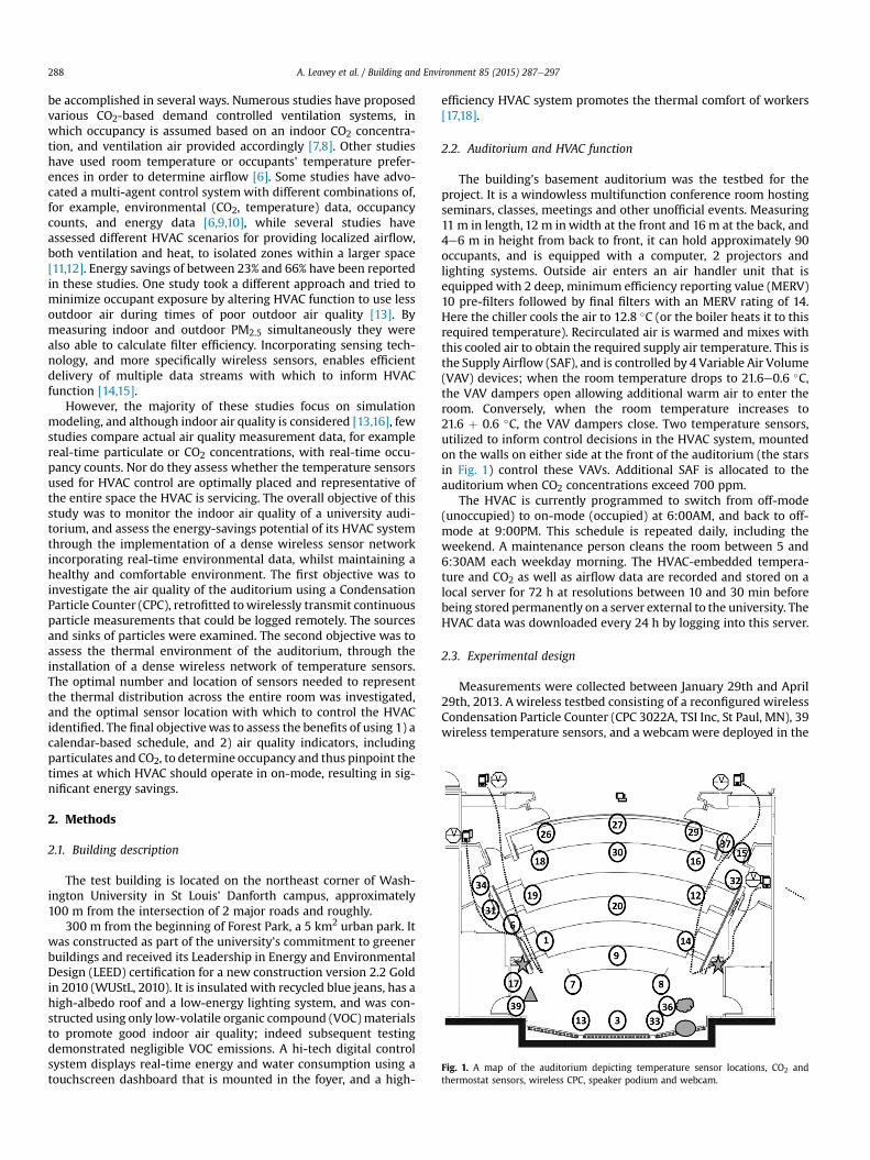
Fig. 1. A map of the auditorium depicting temperature sensor locations, CO2 andthermostat sensors, wireless CPC, speaker podium and webcam.
A. Leavey et al. / Building and Environment 85 (2015) 287e297288
be accomplished in several ways. Numerous studies have proposedvarious CO2-based demand controlled ventilation systems, inwhich occupancy is assumed based on an indoor CO2 concentra-tion, and ventilation air provided accordingly [7,8]. Other studieshave used room temperature or occupants' temperature prefer-ences in order to determine airflow [6]. Some studies have advo-cated a multi-agent control system with different combinations of,for example, environmental (CO2, temperature) data, occupancycounts, and energy data [6,9,10], while several studies haveassessed different HVAC scenarios for providing localized airflow,both ventilation and heat, to isolated zones within a larger space[11,12]. Energy savings of between 23% and 66% have been reportedin these studies. One study took a different approach and tried tominimize occupant exposure by altering HVAC function to use lessoutdoor air during times of poor outdoor air quality [13]. Bymeasuring indoor and outdoor PM2.5 simultaneously they werealso able to calculate filter efficiency. Incorporating sensing tech-nology, and more specifically wireless sensors, enables efficientdelivery of multiple data streams with which to inform HVACfunction [14,15].
However, the majority of these studies focus on simulationmodeling, and although indoor air quality is considered [13,16], fewstudies compare actual air quality measurement data, for examplereal-time particulate or CO2 concentrations, with real-time occu-pancy counts. Nor do they assess whether the temperature sensorsused for HVAC control are optimally placed and representative ofthe entire space the HVAC is servicing. The overall objective of thisstudy was to monitor the indoor air quality of a university audi-torium, and assess the energy-savings potential of its HVAC systemthrough the implementation of a dense wireless sensor networkincorporating real-time environmental data, whilst maintaining ahealthy and comfortable environment. The first objective was toinvestigate the air quality of the auditorium using a CondensationParticle Counter (CPC), retrofitted towirelessly transmit continuousparticle measurements that could be logged remotely. The sourcesand sinks of particles were examined. The second objective was toassess the thermal environment of the auditorium, through theinstallation of a dense wireless network of temperature sensors.The optimal number and location of sensors needed to representthe thermal distribution across the entire room was investigated,and the optimal sensor location with which to control the HVACidentified. The final objectivewas to assess the benefits of using 1) acalendar-based schedule, and 2) air quality indicators, includingparticulates and CO2, to determine occupancy and thus pinpoint thetimes at which HVAC should operate in on-mode, resulting in sig-nificant energy savings.
2. Methods
2.1. Building description
The test building is located on the northeast corner of Wash-ington University in St Louis' Danforth campus, approximately100 m from the intersection of 2 major roads and roughly.
300 m from the beginning of Forest Park, a 5 km2 urban park. Itwas constructed as part of the university's commitment to greenerbuildings and received its Leadership in Energy and EnvironmentalDesign (LEED) certification for a new construction version 2.2 Goldin 2010 (WUStL, 2010). It is insulated with recycled blue jeans, has ahigh-albedo roof and a low-energy lighting system, and was con-structed using only low-volatile organic compound (VOC)materialsto promote good indoor air quality; indeed subsequent testingdemonstrated negligible VOC emissions. A hi-tech digital controlsystem displays real-time energy and water consumption using atouchscreen dashboard that is mounted in the foyer, and a high-
efficiency HVAC system promotes the thermal comfort of workers[17,18].
2.2. Auditorium and HVAC function
The building's basement auditorium was the testbed for theproject. It is a windowless multifunction conference room hostingseminars, classes, meetings and other unofficial events. Measuring11 m in length, 12 m inwidth at the front and 16 m at the back, and4e6 m in height from back to front, it can hold approximately 90occupants, and is equipped with a computer, 2 projectors andlighting systems. Outside air enters an air handler unit that isequipped with 2 deep, minimum efficiency reporting value (MERV)10 pre-filters followed by final filters with an MERV rating of 14.Here the chiller cools the air to 12.8 �C (or the boiler heats it to thisrequired temperature). Recirculated air is warmed and mixes withthis cooled air to obtain the required supply air temperature. This isthe Supply Airflow (SAF), and is controlled by 4 Variable Air Volume(VAV) devices; when the room temperature drops to 21.6e0.6 �C,the VAV dampers open allowing additional warm air to enter theroom. Conversely, when the room temperature increases to21.6 þ 0.6 �C, the VAV dampers close. Two temperature sensors,utilized to inform control decisions in the HVAC system, mountedon the walls on either side at the front of the auditorium (the starsin Fig. 1) control these VAVs. Additional SAF is allocated to theauditorium when CO2 concentrations exceed 700 ppm.
The HVAC is currently programmed to switch from off-mode(unoccupied) to on-mode (occupied) at 6:00AM, and back to off-mode at 9:00PM. This schedule is repeated daily, including theweekend. A maintenance person cleans the room between 5 and6:30AM each weekday morning. The HVAC-embedded tempera-ture and CO2 as well as airflow data are recorded and stored on alocal server for 72 h at resolutions between 10 and 30 min beforebeing stored permanently on a server external to the university. TheHVAC data was downloaded every 24 h by logging into this server.
2.3. Experimental design
Measurements were collected between January 29th and April29th, 2013. A wireless testbed consisting of a reconfigured wirelessCondensation Particle Counter (CPC 3022A, TSI Inc, St Paul, MN), 39wireless temperature sensors, and a webcamwere deployed in the
A. Leavey et al. / Building and Environment 85 (2015) 287e297 289
auditorium to monitor the air quality, temperature, and occupancyof the room. This was in addition to the two HVAC-embedded CO2and temperature sensors that were used to inform HVAC operation,as well as airflow data that was collected every 15 min. Together, acomprehensive profile of the air quality and thermal variability ofthe auditorium was assessed. Fig. 1 presents a schematic of theauditorium highlighting the location of the HVAC VAVs, tempera-ture sensors, CPC and seating arrangements. The following para-graphs present further information regarding each of theinstruments deployed in the auditorium.
2.3.1. Particle countsA CPC 3022A counts airborne particle numbers with a diameter
between 0.07 and 3 mm, at concentrations up to 9.99 � 106 cm�3
(with an accuracy of ±10% for concentrations up to 5 � 105 cm�3),using butanol and photometric technology. For this project the CPCwas retrofitted, using its RS-232 connection, with a connectBlueOBS-421 classic Bluetooth RS-232 cable replacement device. Inaddition to the wire replacement, some reverse engineering of theCPC's protocol to extract and record the data into a correlatedformat with the temperature readings (described in the next sec-tion) was performed, which is more useful and easier to work withthan attempting to combine the data after the fact. Data weretransmitted wirelessly, and detected and recorded using packetsniffing software on a base station computer equipped with asimilar Bluetooth device for the connection to the laptop RS-232port, and located under the speaker podium at the front of theroom. This computer logged and correlated the data and uploadedit to a cloud server thus ensuring continuous collection and long-term storage of data with increased ease and security, as well asoff-site accessibility from any shared computer. Particle data werecollected every 20 s. To ensure that any instrument error would beimmediately detected, the softwarewas configured to send an errorwarning to a predetermined email address so that any issues couldbe promptly resolved. It would be possible to collect data frommultiple wireless CPCs using just one bay station.
2.3.2. Temperature sensor networkThirty-nine wireless temperature sensors - White-Rodgers
F145RF-1600, manufactured by Emerson, were repurposed fordistributed monitoring and positioned along the walls, desks andpodium of the auditorium at different heights (0.5e3m), in order tocapture real-time fine-grained spatiotemporal dynamics of theroom. These sensors communicate using Bluetooth™ v2.1 EDR.Each sensor required modifications to the firmware in order toremove the limit on the number of supported sensors that could beconnected to the system (4), and to enable the passing of sensor IDto the base station. Although the address of each sensor is known,the header that is transmitted to the receiver with this informationwas stripped at the hardware level prior to being passed to the basestation. These sensors have an accuracy of ±0.5 �C. When theydetected a temperature change greater than 0.1 �C, the new tem-perature value was transmitted to the base station, which was thensent to a database in the cloud. In the event that no temperaturechange occurred, a response was sent every half hour, to assure thehost that the sensor was still operational. All of the temperaturesensors were battery-operated enabling them to be placedthroughout the room at minimum cost. This temperature networkwas in addition to the two HVAC-embedded temperature ther-mostats currently used to inform HVAC operation. Although 39wireless sensors were deployed in the auditorium, only thosesensors installed on desks and on walls near to the ground, anddisplaying stable measurements (25 sensors) were included in thisanalysis since they best represented occupancy comfort. Thosesensors installed on the upper walls and ceilings will be analyzed in
future work to generate a more comprehensive temperature dis-tribution profile of the auditorium.
2.3.3. Occupancy detectionAWi-Fi enabled webcam (DCS-2132L) manufactured by D-Link,
was deployed at the front of the auditorium to monitor occupancyat a rate of 1 image every 15 min. The optimal location for thewebcam was decided by installing it in multiple locations andcomparing the seats captured. The location finally decided uponwas able to capture the most relevant seating: the auditoriumtended to fill up on the right-hand side first (the side where thespeaker stood), in the middle and back. The front tended to fill-upmore slowly, especially the very front seats and the ones on the left.More often than not the auditorium was not filled to full-capacityand therefore many of the front and left-hand seats would gounoccupied.
From its optimal location, the camera was able to capture over90% of the seating capacity of the auditorium. These images werethen sent to the backend server over a campus-wide Wi-Finetwork. The number and location of occupants were countedoffline by visual inspection of the images. When an image con-tained many occupants it was printed out and a head count wasperformed bymanually checking-off each occupant with a pen. Theprocess was made easier by the date and time stamp included oneach image, which allowed the counts to be easily cross-checked.The random cross-checking that was subsequently performed en-sures that the final occupancy counts are presented withconfidence.
2.4. Data analysis
All data were checked for accuracy prior to analysis for qualitycontrol purposes. A glitch in the system caused some of the auto-mated airflow and CO2 data to output replicated data which had tobe removed, and instrument error meant that 5 days of particledata were lost. The temperature sensors collected 3 measurementsat a time, for validity purposes. If any of these temperatures devi-ated too far from the average of the 3 they were rejected and themeasurement cycle repeated. If too many were rejected, the sensorwould send a failure message indicating transducer failure. Thusany malfunctioning sensors were identified and removed from thenetwork. Of the retained temperature sensors 7 days were lost dueto system error.
The webcam was able to capture more than 90% of the occu-pancy of the auditorium, and therefore a slight underestimation ofoccupants is possible. Each variable was recorded at differenttemporal resolutions; data was therefore converted to hourly av-erages, the lowest common denominator. All but 2 instances ofoccupancy occurred during the weekday. For this reason analysisand reported results pertain only to weekday data. The final datasetused in this study consisted of 25 temperature sensors, 2 HVAC-embedded temperature and CO2 sensors, 1 wireless CPC and 1webcam. Several matrices were generated using the retainedweekday data for further analysis. All analysis and graphics wereperformed using R (version 2.11.0, R Foundation for StatisticalComputing), MATLAB (version 7.10 R2010a, The MathWorks, Inc.),and SigmaPlot (version 11.0, Systat Software, Inc.).
3. Results and discussion
3.1. General description
Themean outdoor temperature during the measurement periodwas 6.5 �C, and ranged from �6.5e29.2 �C. Mean airflow into theauditorium from the HVAC system was approximately 0.118 m3/s
Fig. 2. Weekday hourly average occupancy counts (top), particle number and NOX
concentrations (secondary axis) (bottom).
A. Leavey et al. / Building and Environment 85 (2015) 287e297290
(off-mode) to 1.180 m3/s (on-mode), increasing to more than1.89 m3/s with high occupancy numbers. Out of almost 3 months ofdata (2046 h), the roomwas occupied for just 304 h, approximately14.8% of the time. When only the on-mode is considered, this in-creases to 20%. It is also important to note that while occupancylevels ranged from 0 to 82 persons, just under the full capacity ofthe auditorium, 36% of the time that it was occupied, this was byonly one person, predominantly a maintenance or cleaning crewmember, and 62% of the time it was occupied by fewer than 10people. Mean CO2 concentrations were approximately 456 ppm (SD36), while particle numbers and temperature (HVAC-embeddedsensor) were approximately 1110 cm�3 (SD 2093) and 20.5 �C (SD0.74) respectively. These concentrations tended to increase withhigher occupancy rates, although for particle numbers the rela-tionship was more complicated.
3.2. Particle number concentrations
Particulate matter is an important ambient air quality indicatorfor which legally-binding standards exist [19]. Indoor particulatematter comprises primary particles that have infiltrated from theoutdoors, primary particles generated from indoor sources, andsecondary particles generated from precursors emitted both in-doors and outdoors [20]. The influence of ambient outdoor aerosolson the indoor environment depends on a particle's ability topenetrate a building, and its fate once inside. The Infiltration Factoris defined as the equilibrium fraction of ambient particles thatpenetrate indoors and remain suspended [21], and depends on theambient outdoor concentration, the strength of indoor sources,structural characteristics of the building and building condition(presence of gaps, cracks), air exchange rates, indoor flow patterns,types of ventilation, the position and size of inlet and outlet vents,the presence of windows and double-glazing, construction mate-rials of the walls, the characteristics of the wind system operatingaround the house, and the penetration coefficient of the particle[21e24]. A particle's composition dictates how far it is transportedaway from source and how readily it can penetrate into a building:those comprised of volatile species will experience reduced infil-tration due to volatilization, while particles comprised predomi-nantly of elemental carbon will infiltrate more readily [25]. Indoor/outdoor studies have demonstrated reduced penetration rates forthe smallest (<100 nm) and largest (>1000 nm) particles [21,24].Once inside, attenuation, deposition and resuspension becomedominant processes [26]. The rate of attenuation and depositiondepends on the presence of air filtration systems, the size, quantityand nature of interior furnishings, surface space, cleaning activities,and the type of floor material, for example carpet or linoleum[27,28]. Conversely, resuspension is caused by the presence ofpeople, and cleaning activities such as sweeping and vacuuming, orthe use of fans [26].
A CPC was successfully configured to wirelessly transmitcontinuous particle number data to a base station located on theother side of the auditorium. This data was used to assess theaerosol environment within the auditorium e identifying anyparticle number trends and possible sources and sinks. In order toascertain these trends it is important to understand whether out-door particle concentrations may be influencing indoor concen-trations. This was achieved by comparing nitrogen oxides (NOX)concentrations measured at a fixed site monitor (FSM) located4.8 km away in Forest Park and operated by the United StatesEnvironmental Protection Agency (USEPA). The correlation be-tween NOX and particle numbers, especially ultrafine particles(UFP) (particles with an aerodynamic diameter below 0.1 mm), iswell established, and is often stronger than the correlation betweenUFP and other particle metrics. This is particularly true within
urban areas, due to their shared source: vehicle exhaust emissions[29e32].
Fig. 2 compares hourly averages for the 3 months of particlenumber data, outdoor NOX concentrations from the same timeperiod, and occupancy counts. A decrease in particle number con-centrations can be observed from late night/early hours of themorning until around 6:00AM where a steady increase until8:00AM is noted. This increase in concentrations somewhat coin-cide, with some time delay, with an increase in outdoor NOX con-centrations which begin to increase at approximately 4:00AM,peaking around 7:00AM, indicative of morning rush hour. However,the peak also directly coincides with the HVAC switching from off-to on-mode at 6:00AM. It is around this time that the auditoriumalso receives its daily cleaning. The 2 principal peaks in particlenumber counts occur at 11:00AM and 3:00PM, which correspondswith the most common times for well-attended classes and semi-nars, demonstrated by the corresponding occupancy data. Particlenumbers continue to decline during the late afternoon and eveninguntil around 9:00PM when they begin to increase again. Despitethe slight increase in NOX concentrations around this time, it isunlikely to have caused the peaks observed indoors. This is how-ever, also the time when the HVAC switches from on-to off-mode.The hourly data indicates that the principal sources/activitiesinfluencing particle numbers are occupancy, or activities occurringduring occupancy, and HVAC mode change. The auditorium ap-pears to be by and large unaffected by outside influences. Toconfirm this, Pearson's product correlation was performed forhourly particle number and NOX data. This was performed multipletimes for different time lags (real-time, 1-, 2-, and 3-h delays). Nostatistical correlationwas observed. Similar analysis was conductedbetween UFP and outdoor ambient temperature. Again no statis-tical correlation was observed.
A. Leavey et al. / Building and Environment 85 (2015) 287e297 291
Fig. 3 presents a time-series depicting particle number counts,occupancy and airflow in the auditorium during a typical work-week. The highest concentrations of particles occurred during highoccupancy events: concentrations as high as 27,000 cm�3 and12,500 cm�3 were observed for seminars with 39 and 42 occupantsrespectively. In fact the highest observed particle number counts of39,781 cm�3 occurred during a high-occupancy (68) seminar (datanot shown). A projector, located by Sensor 27 in Fig. 1, operatedwhenever the room was occupied, and the lights were always on;the main doors were also closed. A CPC 3007 (TSI Inc.) was used toidentify any particle hotspots within the unoccupied auditorium.The projector and lights were switched on andmultiple continuousmeasurements were collected. Mean concentrations were approx-imately 579 cm�3 (SD 21.8 cm�3) and 535 cm�3 (SD 20.1 cm�3) atthe front and back of the auditorium, respectively. Further mea-surements were made 90 min later, thus allowing the projector towarm up, at different locations in the room and by the projector.Mean concentrations next to the projector increased slightly to712 cm�3 (SD 76.1 cm�3); similar concentrations were measuredaround the room. Next, the 2 main doors of the room were closedand further measurements were collected 30 min later. Meanconcentrations increased to 895 cm�3 (SD 34.6 cm�3) (by theprojector) to 916 cm�3 (SD 25.5 cm�3) (at the front of the roomwhere the CPC 3022A had been positioned). While a slight increasein particle concentrations was observed when the projector wasoperating, concentrations did not increase to the levels observedduring times of occupancy. A slight increase in particles was alsoobservedwhen themain doors were closed. This is likely due to the
Fig. 3. Time-series of particle number counts (cm�3) and airflow (m3/s) (bottom) andoccupancy (counts) and NOX (mgm�3) (top). Particle number counts coincide with thefollowing events: 1) the HVAC switching to off-mode; 2) a class of 5 people; 3) HVACswitching to off-mode; 4) a class of 10 people; 5) a class of 9 people; 6) the HVACswitching to on-mode; 7) a seminar of 25 people with pizza; 8) a seminar of 39 people;9) a seminar of 42 people; 10) HVAC switching to off-mode; 11) HVAC switching to on-mode. The missing data points observed for NOX and airflow are due to instrumentfailure.
reduced airflow into and out of the room. Again, the projector doesnot seem the likely source of such high levels of particles observedduring occupancy. Another activity that frequently occurred whilstthe auditorium was occupied was the consumption of food anddrink, both hot and cold. Pizza and coffee was served on occasion,but by no means every time. Hot food has been identified as asource of particles [33,34]; however most studies focus on theparticles generated during the cooking process and few have re-ported particle concentrations from standing cooked food. Tosummarize: increased particle counts occurred under high-occupancy events, either from the occupants themselves or theiractivities, and when the HVAC switched between modes; routinemaintenance and cleaning of the room may have been anotherpotential source. No other sources from nearby rooms wereobserved.
While outdoor conditions are indeed important for naturally-ventilated buildings, the auditorium is a windowless subterra-nean room recently constructed usingmodernmaterials. The room,as well as the building, is mechanically ventilated using a modernHVAC system equipped with 2 sets of high-efficiency filters (MERVratings 10 and 14). The higher the MERV rating, the more efficientthese filters are at preventing particle filtration, and efficiencieshave been reported by Orch et al. [35] for particles between 0.001and 10 mm in size. Given these characteristics, it is not surprisingthat the results of this study indicated minimal outside interfer-ence. This finding is also supported by Wang et al. [36] who statethat outdoor particle concentrations should not be used toapproximate indoor concentrations for commercial buildingsequipped with HVAC. However, spikes in particle concentrationsfrequently coincided with times the HVAC switched betweenmodes. Studies have reported various HVAC components as suc-cessful particle deposition sites due to impaction and gravitationalsettling, for example on the heat exchangers [37], on the ceiling,walls and floor of ducts [38,39], on the filters [40], and as a surfacefor microbial deposition and growth [39,41]. Although HVAC issuccessful at removing particles from the outdoor air, especiallywith the installation of high-efficiency filters [42], Jeong et al. [38]determined that a large fraction of inhalable particles may enter abuilding room if the HVAC system is of moderate length with fewfittings. Their study also demonstrated that particles that havedeposited in the HVAC system, but have low adhesion, may be re-suspended during the initiation of airflow, for example when anHVAC system switches from off-to on-mode, and that the degree ofresuspension depends on the particle surface loading. Bonetta et al.[41] attributed the daily spike in indoor fungal and bacterial countsto the HVAC system switching between modes. They speculatedthat microorganisms proliferate on the filter and in the ducts dur-ing nighttime off-mode then enter the room air as airflow in-creases. This may explain the 6:00AM spikes observed in this study,when the HVAC switched to on-mode. Another spike in particleconcentrations was frequently observed when the HVAC switchedto off-mode. Although fewer studies have examined this, it isplausible that as the HVAC enters off-mode and exfiltration slows,particles are no longer being removed and so increased concen-trations are detected by the CPC. In addition to the HVAC system,other particle sources included certain chemicals and paints, hotfood, cleaning (both from the product used and the actual physicalactivity), and people/occupants. In fact, people are important interms of both generating particles, for example bioaerosols [41],and resuspending them, from mechanical and thermal distur-bances [16]. Secondary organic aerosol (SOA) formation, includingUFP, can occur when condensing ozone-reactive chemicals, emittedby indoor furnishings, building materials and even people, eithernucleate or partition onto already-present particles [43]. HVAC caninfluence SOA formation by modifying ventilation rates and thus
A. Leavey et al. / Building and Environment 85 (2015) 287e297292
the concentration of pre-existing particles within the room; thetemperature of the room, the HVAC filter efficiency and whetherthe filter removes ozone also influence SOA formation [44].
3.3. Temperature variability
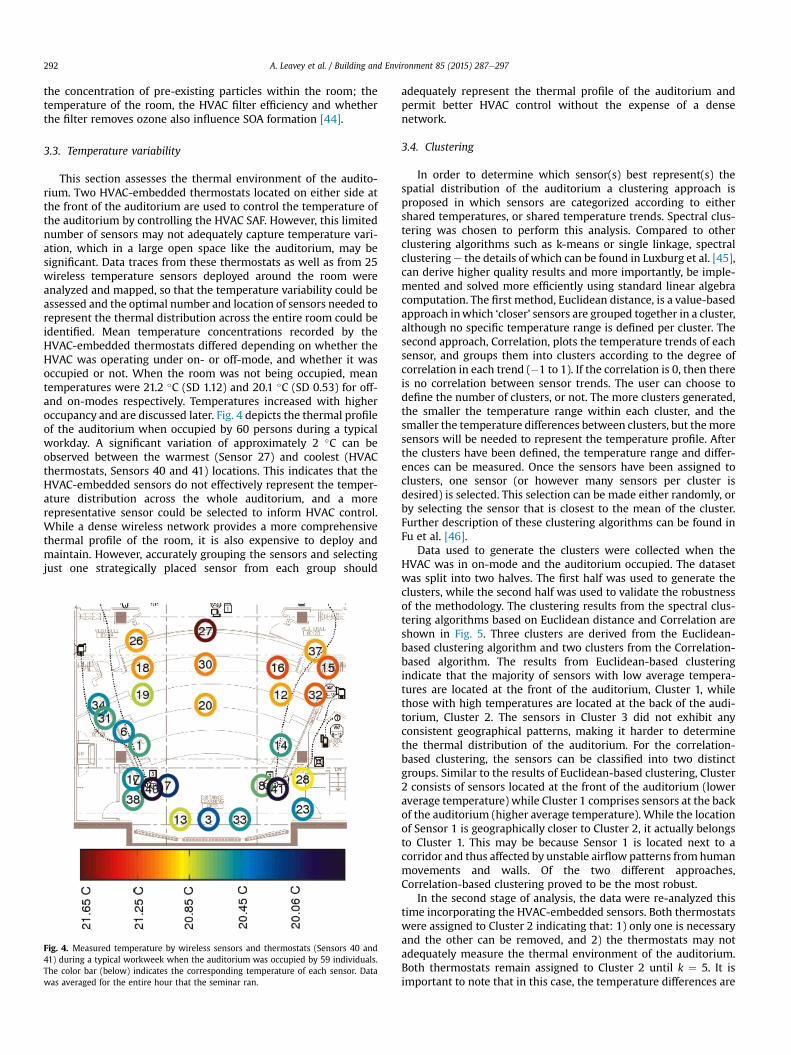
This section assesses the thermal environment of the audito-rium. Two HVAC-embedded thermostats located on either side atthe front of the auditorium are used to control the temperature ofthe auditorium by controlling the HVAC SAF. However, this limitednumber of sensors may not adequately capture temperature vari-ation, which in a large open space like the auditorium, may besignificant. Data traces from these thermostats as well as from 25wireless temperature sensors deployed around the room wereanalyzed and mapped, so that the temperature variability could beassessed and the optimal number and location of sensors needed torepresent the thermal distribution across the entire room could beidentified. Mean temperature concentrations recorded by theHVAC-embedded thermostats differed depending on whether theHVAC was operating under on- or off-mode, and whether it wasoccupied or not. When the room was not being occupied, meantemperatures were 21.2 �C (SD 1.12) and 20.1 �C (SD 0.53) for off-and on-modes respectively. Temperatures increased with higheroccupancy and are discussed later. Fig. 4 depicts the thermal profileof the auditorium when occupied by 60 persons during a typicalworkday. A significant variation of approximately 2 �C can beobserved between the warmest (Sensor 27) and coolest (HVACthermostats, Sensors 40 and 41) locations. This indicates that theHVAC-embedded sensors do not effectively represent the temper-ature distribution across the whole auditorium, and a morerepresentative sensor could be selected to inform HVAC control.While a dense wireless network provides a more comprehensivethermal profile of the room, it is also expensive to deploy andmaintain. However, accurately grouping the sensors and selectingjust one strategically placed sensor from each group should
Fig. 4. Measured temperature by wireless sensors and thermostats (Sensors 40 and41) during a typical workweek when the auditorium was occupied by 59 individuals.The color bar (below) indicates the corresponding temperature of each sensor. Datawas averaged for the entire hour that the seminar ran.
adequately represent the thermal profile of the auditorium andpermit better HVAC control without the expense of a densenetwork.
3.4. Clustering
In order to determine which sensor(s) best represent(s) thespatial distribution of the auditorium a clustering approach isproposed in which sensors are categorized according to eithershared temperatures, or shared temperature trends. Spectral clus-tering was chosen to perform this analysis. Compared to otherclustering algorithms such as k-means or single linkage, spectralclusteringe the details of which can be found in Luxburg et al. [45],can derive higher quality results and more importantly, be imple-mented and solved more efficiently using standard linear algebracomputation. The first method, Euclidean distance, is a value-basedapproach inwhich ‘closer’ sensors are grouped together in a cluster,although no specific temperature range is defined per cluster. Thesecond approach, Correlation, plots the temperature trends of eachsensor, and groups them into clusters according to the degree ofcorrelation in each trend (�1 to 1). If the correlation is 0, then thereis no correlation between sensor trends. The user can choose todefine the number of clusters, or not. The more clusters generated,the smaller the temperature range within each cluster, and thesmaller the temperature differences between clusters, but themoresensors will be needed to represent the temperature profile. Afterthe clusters have been defined, the temperature range and differ-ences can be measured. Once the sensors have been assigned toclusters, one sensor (or however many sensors per cluster isdesired) is selected. This selection can be made either randomly, orby selecting the sensor that is closest to the mean of the cluster.Further description of these clustering algorithms can be found inFu et al. [46].
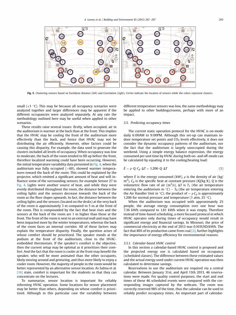
Data used to generate the clusters were collected when theHVAC was in on-mode and the auditorium occupied. The datasetwas split into two halves. The first half was used to generate theclusters, while the second half was used to validate the robustnessof the methodology. The clustering results from the spectral clus-tering algorithms based on Euclidean distance and Correlation areshown in Fig. 5. Three clusters are derived from the Euclidean-based clustering algorithm and two clusters from the Correlation-based algorithm. The results from Euclidean-based clusteringindicate that the majority of sensors with low average tempera-tures are located at the front of the auditorium, Cluster 1, whilethose with high temperatures are located at the back of the audi-torium, Cluster 2. The sensors in Cluster 3 did not exhibit anyconsistent geographical patterns, making it harder to determinethe thermal distribution of the auditorium. For the correlation-based clustering, the sensors can be classified into two distinctgroups. Similar to the results of Euclidean-based clustering, Cluster2 consists of sensors located at the front of the auditorium (loweraverage temperature) while Cluster 1 comprises sensors at the backof the auditorium (higher average temperature). While the locationof Sensor 1 is geographically closer to Cluster 2, it actually belongsto Cluster 1. This may be because Sensor 1 is located next to acorridor and thus affected by unstable airflow patterns fromhumanmovements and walls. Of the two different approaches,Correlation-based clustering proved to be the most robust.
In the second stage of analysis, the data were re-analyzed thistime incorporating the HVAC-embedded sensors. Both thermostatswere assigned to Cluster 2 indicating that: 1) only one is necessaryand the other can be removed, and 2) the thermostats may notadequately measure the thermal environment of the auditorium.Both thermostats remain assigned to Cluster 2 until k ¼ 5. It isimportant to note that in this case, the temperature differences are
Fig. 5. Clustering sensors based on Euclidean distance (left) and Correlation (right). Circles indicate the location of sensors while the colors represent clusters.
A. Leavey et al. / Building and Environment 85 (2015) 287e297 293
small (<1 �C). This may be because all occupancy scenarios wereanalyzed together and larger differences may be apparent if thedifferent occupancies were analyzed separately. At any rate themethodology outlined here may be useful when applied to otherscenarios.
These results raise several issues: firstly, when occupied, air inthe auditorium is warmer at the back than at the front. This impliesthat the HVAC may be cooling the front of the auditorium moreeffectively than the back, and hence that HVAC may not bedistributing the air efficiently. However, other factors could becausing this disparity. For example, the data used to generate theclusters included all levels of occupancy. When occupancy was lowto moderate, the back of the room tended to fill up before the front,therefore localized warming could have been occurring. However,the initial temperature variability data presented in Fig. 4, when theauditorium was fully occupied (þ60), showed warmer tempera-tures toward the back of the room. This could be explained by theprojector, which emitted a significant amount of heat and will in-fluence some of the surrounding sensors, for example Sensor 27 inFig. 4. Lights were another source of heat, and while they wereevenly distributed throughout the room, the distance between theceiling lights and the sensors decrease towards the back of theroom as the floor slopes upwards. In fact, the distance between theceiling lights and the sensors (located on the desks) at the very backof the room is approximately 3 m compared to 5 m at the front ofthe room. This is compounded by the fact that heat rises and thesensors at the back of the room are 1 m higher than those at thefront. The front of the room is next to an external wall andmay havebeen impacted more by the winter temperatures, whereas the backof the room faces an internal corridor. All of these factors mayexplain the temperature disparity. Finally, the question arises ofwhose comfort should be prioritized. The speaker stands at thepodium at the front of the auditorium, close to the HVAC-embedded thermostats. If the speaker's comfort is the objective,then the current setup may be optimal as it prioritizes their com-fort. And the fact that the room is cooler at the frontmay benefit thespeaker, who will be more animated than the other occupants,likely moving around and gesturing, and thus more likely to enjoy acooler room. However, the majority of people in the roomwould bebetter represented by an alternative sensor location. As Salma et al.[16] state, comfort is important for the students so that they canconcentrate on the lectures.
To summarize, sensor location is important for reliablyinforming HVAC operation. Some locations for sensor placementmay be better than others, depending on whose comfort is priori-tized. Although in this particular case the variability between
different temperature sensors was low, the samemethodologymaybe applied to other buildings/rooms, perhaps with more of animpact.
3.5. Predicting occupancy times
The current static operation protocol for the HVAC is on-modedaily 6:00AM to 9:00PM. Although this set-up can maintain in-door temperature set points and CO2 levels effectively, it does notconsider the dynamic occupancy patterns of the auditorium, northe fact that the auditorium is largely unoccupied during theweekend. Using a simple energy balance expression, the energyconsumed per unit time byHVAC during both on- and off-mode canbe calculated by equating it to the cooling/heating load:
_E ¼ r$Q$Cp$DT ¼ 1.206$Q$DT (1)
where _E is the energy consumed (kW), r is the density of air (kg/m3), Cp is the specific heat at constant pressure (KJ/kg K), Q is thevolumetric flow rate of air (m3/s), DT is T1 (the air temperatureentering the auditorium in �C) e T0 (the air temperature enteringthe Air Handler Unit in �C); the product of ¼ r·Cp is approximately1.206 for normal pressure and temperature (1 atm, 25 �C).
When the auditorium was occupied with approximately 25people, the average energy consumption over one hour was7.36 kWh compared to 1.81 kWh when it was empty. Thereforeinstead of time-based scheduling, a more focused protocol inwhichHVAC operates only during times of occupancy would result insignificant energy and financial savings. In Missouri, the price ofcommercial electricity at the end of 2013 was 0.103USD/kWh. Thefact that 80% of its production came from coal [2], further highlightsthe importance of energy efficiency for environmental reasons.
3.5.1. Calendar-based HVAC controlIn this section a calendar-based HVAC control is proposed and
the projected energy use is calculated based on occupancy(scheduled classes). The difference between these estimated valuesand the actual energy used under current HVAC operationwas thencalculated to determine savings.
Reservations to use the auditorium are required via a centralcalendar. Between January 31st, and April 13th 2013, 46 reserva-tions were made. For quality control purposes, the start and endtimes of these 46 scheduled events were compared with the cor-responding images captured by the webcam. The room wascorrectly reserved 98% of the time, thus the calendar can be used toreliably predict occupancy times. An important part of calendar-
Fig. 6. A cumulative density function depicting the time it takes for temperatures tostabilize in the comfort zone.
A. Leavey et al. / Building and Environment 85 (2015) 287e297294
based HVAC scheduling is understanding the time required toprecondition, i.e. turn-on the HVAC so that the room is at acomfortable temperature before individuals enter. If HVAC startspreconditioning too early, energymay bewasted providing thermalcomfort to an empty room. Conversely, if preconditioning beginstoo late occupants may experience discomfort, which compromisesthe basic objective of the HVAC system. In order to ascertain anappropriate way of manipulating the HVAC between modes, apreconditioning time of (tp) was identified from data recorded bythe HVAC-embedded thermostats, so that the HVAC would operatetp prior to auditorium occupancy. The preconditioning time wasdefined as the time it takes for temperatures to stabilize in thecomfort range 21 ± 1 �C. When the HVAC switched to on-mode at6:00AM, the temperature in the auditorium fluctuated in and out ofthis comfort range. Using the daily temperature dataset, the time ittook for the temperature to reach the occupancy comfort range andremain there without variation was recorded. The results are pre-sented as a distribution in Fig. 6, demonstrating that 90% of the timeit takes 178 min for the temperature to stabilize in the occupancycomfort range. Therefore the HVAC should switch to on-modeapproximately 178 min prior to an event.
The next consideration was when to return the HVAC to off-mode. The most efficient route is selecting the end time of theevent, providing the interval before the next scheduled event is
Fig. 7. Comparing the on-mode operation of the HVAC for the current scenario with that oHVAC is operating in on-mode. (Right): the energy savings garnered by implementing each oand the error bars represent the variation between these days.
longer that tp. The calendar-based scheduling of HVAC includes thefollowing energy saving rules:
1) The HVAC should switch to on-mode at tp prior to the occu-pancy event.
2) The HVAC should switch to off-mode immediately after theevent. If multiple events are scheduled, apply Rule 3.
3) The HVAC should only remain in on-mode if the interval be-tween events is shorter than tp to avoid oscillation (the frequentswitching between modes).
4) The HVAC should be set to off-mode during the weekend, unlessan event is scheduled.
Potential energy savings were calculated using data that hadbeen collected between February 10th and February 17th, repre-senting a typical working week in the auditorium. Actual energyusage during that week was compared to what the energy usagewould be if these energy saving rules were implemented. Sevenevents occurred between Monday and Friday, and occupanciesranged from approximately 10 to 70 people. By applying Rules 1)and 2), HVAC turns on at tp (178 min) before the event to precon-dition the auditorium and turns off immediately after the event. OnFriday there were two events separated by a time interval of150 min, which is shorter than tp. Thus Rule 3) is applied and theHVAC remains on for the 150 min between the two events. Rule 4)is applied for the weekend, and the HVAC is switched offcompletely. Fig. 7 presents the energy saved when each of theserules are applied. Employing Rule 1 produced an 8% reduction inenergy consumption; Rule 2 and a 37% reduction was observed. Noenergy savings were garnered by applying Rule 3, as the HVACoperated as it would in its current operation. Rule 4 saved 34% ofenergy and would be easily implemented. If all rules were applied,the total energy savings would be 79%.
Most events in the auditorium finished before 4:00PM, afterwhich, according to Rule 2), the HVAC may return to off-mode,5 h earlier than the current protocol. Increased energy savingscan be made by scheduling events close together. That way theHVAC can remain in on-mode for a shorter total period of time andexpending energy to precondition is limited. If the calendar isconsistent throughout the weeks, an algorithm may be written sothat HVAC operation becomes automated and limited additionalman-power is needed. In Missouri, more than 80% of the electricitygenerated comes from coal, a reliance that has been increasing overthe years [1]. Hence reducing HVAC energy consumption candirectly reduce CO2 emissions.
f calendar-based scheduling (left); the columns represent the times during which thef the energy saving rules. The columns depict the mean energy savings across the week,
Time (Hr)0 5 10 15 20 25
CO
2 )
mpp(snoitartnecnoc
430
440
450
460
470
480
490
500
510
Occupancy (counts)
0
2
4
6
8
10
12
14COOccupancy
Time 09:00 10:00 11:00 12:00 13:00 14:00
CO
2)
mpp(snoitartnecnoc
400
450
500
550
600
650
700
750
800
Occupancy (counts)
0
20
40
60
80
100CO2Occupancy
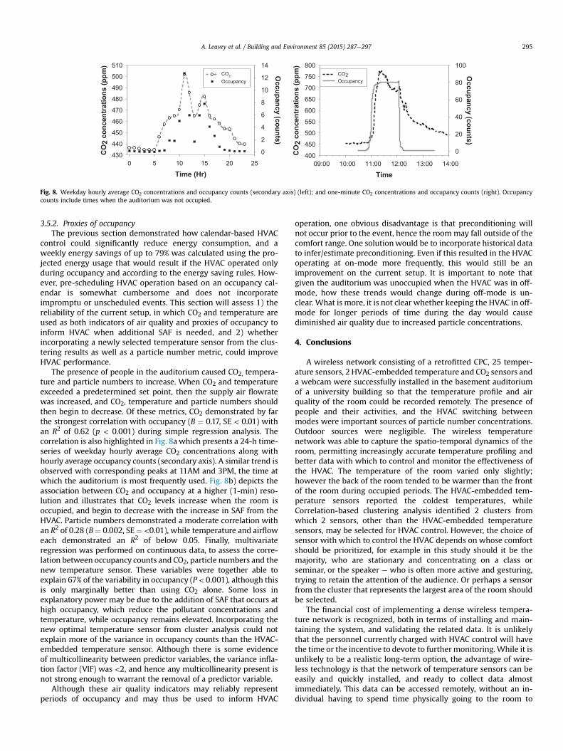
Fig. 8. Weekday hourly average CO2 concentrations and occupancy counts (secondary axis) (left); and one-minute CO2 concentrations and occupancy counts (right). Occupancycounts include times when the auditorium was not occupied.
A. Leavey et al. / Building and Environment 85 (2015) 287e297 295
3.5.2. Proxies of occupancyThe previous section demonstrated how calendar-based HVAC
control could significantly reduce energy consumption, and aweekly energy savings of up to 79% was calculated using the pro-jected energy usage that would result if the HVAC operated onlyduring occupancy and according to the energy saving rules. How-ever, pre-scheduling HVAC operation based on an occupancy cal-endar is somewhat cumbersome and does not incorporateimpromptu or unscheduled events. This section will assess 1) thereliability of the current setup, in which CO2 and temperature areused as both indicators of air quality and proxies of occupancy toinform HVAC when additional SAF is needed, and 2) whetherincorporating a newly selected temperature sensor from the clus-tering results as well as a particle number metric, could improveHVAC performance.
The presence of people in the auditorium caused CO2, tempera-ture and particle numbers to increase. When CO2 and temperatureexceeded a predetermined set point, then the supply air flowratewas increased, and CO2, temperature and particle numbers shouldthen begin to decrease. Of these metrics, CO2 demonstrated by farthe strongest correlation with occupancy (B ¼ 0.17, SE < 0.01) withan R2 of 0.62 (p < 0.001) during simple regression analysis. Thecorrelation is also highlighted in Fig. 8a which presents a 24-h time-series of weekday hourly average CO2 concentrations along withhourly average occupancy counts (secondary axis). A similar trend isobserved with corresponding peaks at 11AM and 3PM, the time atwhich the auditorium is most frequently used. Fig. 8b) depicts theassociation between CO2 and occupancy at a higher (1-min) reso-lution and illustrates that CO2 levels increase when the room isoccupied, and begin to decrease with the increase in SAF from theHVAC. Particle numbers demonstrated a moderate correlation withan R2 of 0.28 (B¼ 0.002, SE¼ <0.01), while temperature and airfloweach demonstrated an R2 of below 0.05. Finally, multivariateregression was performed on continuous data, to assess the corre-lation between occupancy counts and CO2, particle numbers and thenew temperature sensor. These variables were together able toexplain 67% of the variability in occupancy (P < 0.001), although thisis only marginally better than using CO2 alone. Some loss inexplanatory power may be due to the addition of SAF that occurs athigh occupancy, which reduce the pollutant concentrations andtemperature, while occupancy remains elevated. Incorporating thenew optimal temperature sensor from cluster analysis could notexplain more of the variance in occupancy counts than the HVAC-embedded temperature sensor. Although there is some evidenceof multicollinearity between predictor variables, the variance infla-tion factor (VIF) was <2, and hence any multicollinearity present isnot strong enough to warrant the removal of a predictor variable.
Although these air quality indicators may reliably representperiods of occupancy and may thus be used to inform HVAC
operation, one obvious disadvantage is that preconditioning willnot occur prior to the event, hence the roommay fall outside of thecomfort range. One solutionwould be to incorporate historical datato infer/estimate preconditioning. Even if this resulted in the HVACoperating at on-mode more frequently, this would still be animprovement on the current setup. It is important to note thatgiven the auditorium was unoccupied when the HVAC was in off-mode, how these trends would change during off-mode is un-clear. What is more, it is not clear whether keeping the HVAC in off-mode for longer periods of time during the day would causediminished air quality due to increased particle concentrations.
4. Conclusions
A wireless network consisting of a retrofitted CPC, 25 temper-ature sensors, 2 HVAC-embedded temperature and CO2 sensors anda webcam were successfully installed in the basement auditoriumof a university building so that the temperature profile and airquality of the room could be recorded remotely. The presence ofpeople and their activities, and the HVAC switching betweenmodes were important sources of particle number concentrations.Outdoor sources were negligible. The wireless temperaturenetwork was able to capture the spatio-temporal dynamics of theroom, permitting increasingly accurate temperature profiling andbetter data with which to control and monitor the effectiveness ofthe HVAC. The temperature of the room varied only slightly;however the back of the room tended to be warmer than the frontof the room during occupied periods. The HVAC-embedded tem-perature sensors reported the coldest temperatures, whileCorrelation-based clustering analysis identified 2 clusters fromwhich 2 sensors, other than the HVAC-embedded temperaturesensors, may be selected for HVAC control. However, the choice ofsensor with which to control the HVAC depends on whose comfortshould be prioritized, for example in this study should it be themajority, who are stationary and concentrating on a class orseminar, or the speaker e who is often more active and gesturing,trying to retain the attention of the audience. Or perhaps a sensorfrom the cluster that represents the largest area of the room shouldbe selected.
The financial cost of implementing a dense wireless tempera-ture network is recognized, both in terms of installing and main-taining the system, and validating the related data. It is unlikelythat the personnel currently charged with HVAC control will havethe time or the incentive to devote to furthermonitoring.While it isunlikely to be a realistic long-term option, the advantage of wire-less technology is that the network of temperature sensors can beeasily and quickly installed, and ready to collect data almostimmediately. This data can be accessed remotely, without an in-dividual having to spend time physically going to the room to
A. Leavey et al. / Building and Environment 85 (2015) 287e297296
obtain the data. It causes no disturbance to the occupants of thatroom, as there is no wiring to distract or cause health and safetyconcerns. It is therefore a feasible short-term study, especially in auniversity setting where there is always interest in new projects,from which the thermal profile of a room and the effectiveness ofthe current HVAC operation can be assessed. Similar to this study,clustering analysis may be performed to help identify an optimallocation for temperature sensor, increasing the efficacy of the HVACsystem. Given that HVAC is a huge consumer of energy, improvingits function and potentially reducing the amount of time it needs torun, can result in large energy and financial savings. It would beeven more advantageous if clustering analysis and sensor selectioncould be performed without having to install a dense wirelesstemperature network, but it is unclear at this time how this wouldbe achieved.
In this study, experimental data demonstrated that operatingthe HVAC according to a calendar-based rather that a time-basedschedule resulted in significant energy savings of up to 79%,depending on which energy saving rules were applied, and espe-cially if occupancy events were scheduled close together. Thisshould be considered when future class and seminar timetabling isconducted. Finally, CO2 was observed to be a reliable indicator ofoccupancy, demonstrating the strongest correlation with occu-pancy counts of the different metrics assessed; however particlenumber concentrations and either the HVAC-embedded oroptimally-located temperature sensors may supplement CO2 inpredicting times of occupancy for a more efficient and effectiveHVAC control. Incorporating a particle metric can also identify filterefficiency and improve the air quality of the room.
While the focus of this study was occupancy comfort, and onlythose sensors deemed most likely to affect comfort were includedfor analysis, future work will incorporate the remainder of thesensors to assess the thermal profile and temperature dynamics ofthe auditorium as a whole, and to track more precisely how airmoves through the room. In addition, given the strong temperaturefluctuations that occur in continental climates like Missouri, theoutdoor air temperature should be a factor when considering anyalterations to a time-based approach for HVAC operation, and thiswill also be considered in future work.
Acknowledgments
We thank MAGEEP and ICARES at Washington University in StLouis for support of this work. Partial support for this study wasalso provided by a contract from USEPA through Pegasus Inc.
Nomenclature
CO2 carbon dioxideCPC condensation particle counterHVAC heating ventilation and air conditioningMERV minimum efficiency reporting valueNOX nitrogen oxidesSAF supply airflowSOA secondary organic aerosolUFP ultrafine particlesVAV variable air volumeVOCs volatile organic compounds
References
[1] EIA. International energy statistics. 11.15.2013. http://www.eia.gov/countries/data.cfm.
[2] DOE. Buildings energy data book. 11.13.2013. http://buildingsdatabook.eren.doe.gov/TableView.aspx?table¼1.1.3.
[3] DOE. Buildings energy data book. 11.15.2013. http://buildingsdatabook.eren.doe.gov/TableView.aspx?table¼1.1.4.
[4] ASHRAE. Thermal environmental conditions for human occupancy. AtlantaGA. 2013.
[5] Oldewurtel F, Sturzenegger D, Morari M. Importance of occupancy informa-tion for building climate control. Appl Energy 2013;101:521e32.
[6] Klein L, Kwak J-y, Kavulya G, Jazizadeh F, Becerik-Gerber B, Varakantham P,et al. Coordinating occupant behavior for building energy and comfort man-agement using multi-agent systems. Autom Constr 2012;22:525e36.
[7] Fan Y, Kameishi K, Onishi S, Ito K. Field-based study on the energy-savingeffects of CO2 demand controlled ventilation in an office with application ofenergy recovery ventilators. Energy Build 2014;68:412e22.
[8] Lau J. CO2-Based demand controlled ventilation for variable air volume sys-tems serving multiple zones. Indoor Built Environ 2013;22(5):721e3.
[9] Mathews E, Botha C, Arndt D, Malan A. HVAC control strategies to enhancecomfort and minimise energy usage. Energy Build 2001;33(8):853e63.
[10] Yang R, Wang L. Development of multi-agent system for building energy andcomfort management based on occupant behaviors. Energ Build 2013;56:1e7.
[11] Budaiwi I, Abdou A. HVAC system operational strategies for reduced energyconsumption in buildings with intermittent occupancy: the case of mosques.Energy Convers Manage 2013;73:37e50.
[12] Lo LJ, Novoselac A. Localized air-conditioning with occupancy control in anopen office. Energy Build 2010;42(7):1120e8.
[13] Marsik T, Johnson R. HVAC air-quality model and its use to test a PM2.5 controlstrategy. Build Environ 2008;43(11):1850e7.
[14] Bhattacharya S, Sridevi S, Pitchiah R, editors. Indoor air quality monitoringusing wireless sensor network, Sixth Internat Conf Sens Tech. (ICST), 2012.IEEE; 2012. p. 422e7.
[15] Weng T, Agrawal Y. From buildings to smart buildingsesensing and actuationto improve energy efficiency. Green Electron Comput 2012:36e44.
[16] Salma I, Doszt�aly K, Bors�os T, Süveges B, Weidinger T, Krist�of G, et al. Physicalproperties, chemical composition, sources, spatial distribution and sinks of indooraerosol particles in a university lecture hall. Atmos Environ 2013;64:219e28.
[17] Kerr PH. Brauer Hall e post occupancy energy analysis. St Louis: WashingtonUniversity in St Louis; 2011.
[18] WUSTL, Stephen, Hall Camilla Brauer, Green Hall Preston M. LEED® buildingtour. 2012.
[19] EPA National ambient air quality standards (NAAQS). 12.11.2014. http://www.epa.gov/air/criteria.html.
[20] Polidori A, Fine PM, White V, Kwon PS. Pilot study of high performance airfiltration for classroom applications. Indoor Air 2013;23:185e95.
[21] Hussein T, H€ameri K, Heikkinen MS, Kulmala M. Indoor and outdoor particlesize characterization at a family house in EspooeFinland. Atmos Environ2005;39(20):3697e709.
[22] Chang T-J. Numerical evaluation of the effect of traffic pollution on indoor airquality of a naturally ventilated building. J Air Waste Manage 2002;52(9):1043e53.
[23] Kingham S, Briggs D, Elliott P, Fischer P, Lebret E. Spatial variations in theconcentrations of traffic-related pollutants in indoor and outdoor air inHuddersfield. Engl Atmos Environ 2000;34(6):905e16.
[24] Wallace L, Howard-Reed C. Continuous monitoring of ultrafine, fine, andcoarse particles in a residence for 18 months in 1999e2000. J Air WasteManage 2002;52(7):828e44.
[25] Sarnat SE, Coull BA, Ruiz PA, Koutrakis P, Suh HH. The influences of ambientparticle composition and size on particle infiltration in Los Angeles, CA, res-idences. J Air Waste Manage 2006;56(2):186e96.
[26] Thatcher TL, Layton DW. Deposition, resuspension, and penetration of parti-cles within a residence. Atmos Environ 1995;29(13):1487e97.
[27] He C, Morawska L, Hitchins J, Gilbert D. Contribution from indoor sources toparticle number and mass concentrations in residential houses. Atmos Envi-ron 2004;38(21):3405e15.
[28] Spilak MP, Frederiksen M, Kolarik B, Gunnarsen L. Exposure to ultrafine par-ticles in relation to indoor events and dwelling characteristics. Build Environ2014;74(0):65e74.
[29] Ketzel M, Wåhlin P, Berkowicz R, Palmgren F. Particle and trace gas emissionfactors under urban driving conditions in Copenhagen based on street androof-level observations. Atmos Environ 2003;37(20):2735e49.
[30] Morawska L, Jayaratne E, Mengersen K, Jamriska M, Thomas S. Differences inairborne particle and gaseous concentrations in urban air between weekdaysand weekends. Atmos Environ 2002;36(27):4375e83.
[31] Westerdahl D, Fruin S, Sax T, Fine PM, Sioutas C. Mobile platform measure-ments of ultrafine particles and associated pollutant concentrations on free-ways and residential streets in Los Angeles. Atmos Environ 2005;39(20):3597e610.
[32] Pirjola L, Paasonen P, Pfeiffer D, Hussein T, H€ameri K, Koskentalo T, et al.Dispersion of particles and trace gases nearby a city highway: mobile labo-ratory measurements in Finland. Atmos Environ 2006;40(5):867e79.
[33] Buonanno G, Morawska L, Stabile L. Particle emission factors during cookingactivities. Atmos Environ 2009;43:3235e42.
[35] Orch ZE, Stephens B, Waring MS. Predictions and determinants of size-resolved particle infiltration factors in single-family homes in the US. BuildEnviron 2014;74(0):106e18.
A. Leavey et al. / Building and Environment 85 (2015) 287e297 297
[36] Wang Y, Hopke PK, Chalupa DC, Utell MJ. Long-term characterization of in-door and outdoor ultrafine particles at a commercial building. Environ SciTechnol 2010;44(15):5775e80.
[37] Siegel JA, Nazaroff WW. Predicting particle deposition on HVAC heat ex-changers. Atmos Environ 2003;37(39):5587e96.
[38] Jeong J-W, Bem J, Bahnfleth WP, Freihaut JD, Thran B. Critical review of aerosolparticle transportmodels for buildingHVACducts. J Archit Eng2009;15(3):74e83.
[39] Sippola MR, Nazaroff WW. Experiments measuring particle deposition fromfully developed turbulent flow in ventilation ducts. Aerosol Sci Technol2004;38(9):914e25.
[40] Noris F, Siegel JA, Kinney KA. Evaluation of HVAC filters as a sampling mecha-nism for indoor microbial communities. Atmos Environ 2011;45(2):338e46.
[41] Bonetta S, Bonetta S, Mosso S, Samp�o S, Carraro E. Assessment of microbio-logical indoor air quality in an Italian office building equipped with an HVACsystem. Environ Monit Assess 2010;161(1e4):473e83.
[42] Stephens B, Siegel JA. Ultrafine particle removal by residential heating,ventilating, and air conditioning filters. Indoor Air 2013;23(6):488e97.
[43] Weschler CJ. Ozone's impact on public health: contributions from indoorexposures to ozone and products of ozone-initiated chemistry. Environ HealthPerspect 2006;114(10):1489.
[44] Waring MS, Siegel JA. The influence of HVAC systems on indoor secondaryorganic aerosol formation. Ashrae Trans 2010;116:556e71.
[45] Luxburg U. A tutorial on spectral clustering. Stat Comput 2007;17(4):395e416.
[46] Fu Y, Sha M, Wu C, Kutta A, Leavey A, Lu C, et al. Thermal modeling for a HVACcontrolled real-life auditorium, international conference on distributedcomputing systems. In: International conference on distributed computingsystems, Philadelphia, USA; 2014.