Algebraic Point Set Surfaces

Gael Guennebaud Markus GrossETH Zurich

Figure 1: Illustration of the central features of our algebraic MLS framework. From left to right: efficient handling of very complex pointsets, fast mean curvature evaluation and shading, significantly increased stability in regions of high curvature, sharp features with controlledsharpness. Sample positions are partly highlighted.

Abstract

In this paper we present a new Point Set Surface (PSS) definitionbased on moving least squares (MLS) fitting of algebraic spheres.Our surface representation can be expressed by either a projectionprocedure or in implicit form. The central advantages of our ap-proach compared to existing planar MLS include significantly im-proved stability of the projection under low sampling rates and inthe presence of high curvature. The method can approximate orinterpolate the input point set and naturally handles planar pointclouds. In addition, our approach provides a reliable estimate of themean curvature of the surface at no additional cost and allows forthe robust handling of sharp features and boundaries. It processesa simple point set as input, but can also take significant advantageof surface normals to improve robustness, quality and performance.We also present an novel normal estimation procedure which ex-ploits the properties of the spherical fit for both direction estima-tion and orientation propagation. Very efficient computational pro-cedures enable us to compute the algebraic sphere fitting with up to40 million points per second on latest generation GPUs.

CR Categories: I.3.5 [Computer Graphics]: Computational Ge-ometry and Object Modeling—Curve and surface representations

Keywords: point based graphics, surface representation, movingleast square surfaces, sharp features.

1 IntroductionA key ingredient of most methods in point based graphics is the un-derlying meshless surface representation which computes a contin-uous approximation or interpolation of the input point set. The byfar most important and successful class of such meshless represen-tations are point set surfaces (PSS) [Alexa et al. 2003] combining

high flexibility with ease of implementation. PSS generally definea smooth surface using local moving least-squares (MLS) approxi-mations of the data [Levin 2003]. The degree of the approximationcan easily be controlled, making the approach naturally well suitedto filter noisy input data. In addition, the semi-implicit nature ofthe representation makes PSS an excellent compromise combiningadvantages both of explicit representations, such as parametric sur-faces, and of implicit surfaces [Ohtake et al. 2003].

Since its inception, significant progress has been made to betterunderstand the properties and limitations of MLS [Amenta andKil 2004a,2004b] and to develop efficient computational schemes[Adamson and Alexa 2004]. A central limitation of the robustnessof PSS, however, comes from the plane fit operation that is highlyunstable in regions of high curvature if the sampling rate drops be-low a threshold. Such instabilities include erroneous fits or the lim-ited ability to perform tight approximations of the data. This be-havior sets tight limits to the minimum admissible sampling ratesfor PSS [Amenta and Kil 2004b; Dey et al. 2005].

In this paper we present a novel definition of moving least squaressurfaces called algebraic point set surfaces (APSS). The key ideais to directly fit a higher order algebraic surface [Pratt 1987] ratherthan a plane. For computational efficiency all methods in this paperfocus on algebraic sphere fitting, but the general concept could beapplied to higher order surfaces as well. The main advantage ofthe sphere fitting is its significantly improved stability in situationswhere planar MLS fails. For instance, tight data approximation isaccomplished, spheres perform much better in the correct handlingof sheet separation (figure 3) and exhibit a high degree of stabilityboth in cases of undersampling (figure 2) and for very large weightfunctions. The specific properties of algebraic spheres make APSSsuperior to simple geometric sphere fitting. It allows us to elegantlyhandle planar areas or regions around inflection points as limits inwhich the algebraic sphere naturally degenerates to a plane.

Furthermore, the spherical fitting enables us to design interpolatoryweighting schemes by using weight functions with singularities atzero while overcoming the fairness issue of previous MLS surfaces.The sphere radius naturally serves as a for-free and reliable esti-mate of the mean curvature of the surface. This enables us, forinstance, to compute realtime accessibility shading on large inputobjects (figure 1).

Central to our framework are the numerical procedures to efficientlyperform the sphere fit. For point sets with normals we designed

(a) (b) (c)Figure 2: The undersampled ear of the Stanford bunny (a) usingnormal averaging plane fit (SPSS) with h = 1.8 (b) and our newAPSS with h = 1.7 (c).

a greatly simplified and accelerated algorithm whose core part re-duces to linear least squares. For point sets without normals, weemploy a slightly more expensive fitting scheme to estimate thesurface normals of the input data. In particular, this method al-lows us to improve the normal estimation by [Hoppe et al. 1992].The tighter fit of the sphere requires on average less projection it-erations to achieve the same precision making the approach evenfaster than the most simple plane fit MLS. Our implementation onthe latest generation GPUs features a performance up to 45 millionsof points per second, sufficient to compute a variety of operationson large point sets in realtime.

Finally, we developed a simple and powerful extension of [Fleish-man et al. 2005] to robustly handle sharp features, such as bound-aries and creases, with a built-in sharpness control (figure 1).

2 Related WorkPoint set surfaces were introduced to computer graphics by [Alexaet al. 2003]. The initial definition is based on the stationary setof Levin’s moving least squares (MLS) projection operator [Levin2003]. The iterative projection involves a non-linear optimizationto find the local reference plane, a bivariate polynomial fit and it-eration. By omitting the polynomial fitting step, Amenta and Kil[2004a] showed that the same surface can be defined and computedby weighted centroids and a smooth gradient field. This leads toa significantly simplified implicit surface definition [Adamson andAlexa 2004] and faster algorithms, especially in the presence ofnormals [Alexa and Adamson 2004]. In particular, the projectioncan be accomplished on a plane passing through the weighted av-erage of the neighboring samples with a normal computed from theweighted average of the adjacent normals. In the following we willrefer to this efficient variant as SPSS for Simple PSS.

Boissonnat and Cazals [2000] and more specifically Shen et al.[2004] proposed a similar, purely implicit MLS (IMLS) surface

(a) (b) (c)

Figure 3: Sheet separation with conventional PSS compared to ournew spherical fit: (a) Standard PSS with covariance analysis (or-ange) and normal averaging (green). (b) Our APSS without (or-ange) and with (green) normal constraints. The best plane and bestalgebraic sphere fits for the blue point in the middle are drawn inblue. For this example the normals were computed using our tech-nique from section 5 which can safely propagate the orientationbetween the two sheets (c).

Figure 4: A 2D oriented point set is approximated (left) and in-terpolated (right) using various PSS variants: SPSS (blue), IMLS(red), HPSS (magenta) and our APSS (green).

representation defined by a local weighted average of tangential im-plicit planes attached to each input sample. This implicit surfacedefinition was initially designed to reconstruct polygon soups, butthe point cloud case was recently analyzed by Kolluri [2005] andmade adaptive to the local feature size by Dey et al. [2005]. Notethat in this paper IMLS refers to the simple definition given in [Kol-luri 2005]. If applied without polygon constraints and in the caseof sparse sampling, we found that the surface can grow or shrinksignificantly as a function of the convexity or concavity of the pointcloud. To alleviate this problem, Alexa and Adamson [2006] en-forced convex interpolation of an oriented point set using singularweight functions and Hermite centroid evaluations (HPSS).

Likewise relevant to our research is prior art on normal estimation.Many point based algorithms, including some of the aforedescribedPSS variants, require surface normals. A standard procedure pro-posed by [Hoppe et al. 1992] is to estimate their directions usinga local plane fit followed by a propagation of the orientations us-ing a minimum spanning tree (MST) strategy and a transfer heuris-tic based on normal angles. Extending this technique, Mitra andNguyen [2003] take into account the local curvature and the amountof noise in order to estimate the optimal size of the neighborhoodfor the plane fit step. However, the inherent limitations of the planefit step and the propagation heuristic require a very dense samplingrate in regions of high curvature.

Intrinsically, a PSS can only define a smooth closed manifold sur-face. Even though boundaries could be handled by thresholding anoff-center distance [Adamson and Alexa 2004], obtaining satisfac-tory boundary curves with such an approach is usually difficult oreven impossible. In order to detect and reconstruct sharp creasesand corners in a possibly noisy point cloud, Fleishman et al. [2005]proposed a refitting algorithm that locally classifies the samplesinto multiple pieces of surfaces according to discontinuities of thederivative of the surface. While constituting an important progress,the method requires very dense point clouds, it is rather expensive,and it offers only limited flexibility to the user. Also, potential insta-bilities in the classification can create discontinuous surface parts.A second important approach is the Point-Sampled Cell Complexes[Adamson and Alexa 2006b] which allows to explicitly representsharp features by decomposing the object into cells of different di-mensions. While this approach allows to handle a wide variety ofcases (e.g., non-manifoldness), the decomposition and the balanc-ing of the cells’ influence on the shape of the surface demands effortby the user, making the method unsuitable for some applications.

As we will elaborate in the following sections, the algebraic spherefitting overcomes many of the aforedescribed limitations by the sig-nificantly increased robustness of the fit in the presence of low sam-pling rates and high curvature.

3 Overview of the APSS framework

Given a set of points P = {pi ∈ Rd}, we define a smooth surfaceSP approximating P using a moving least squares spherical fit tothe data. Our approach handles both simple point clouds and point

c

pi

pi

pj

c c

u(p )i

u(x)u(m)

mx=q

0

q1

(a) (b) (c) (d)

Nor

mal

dir

ectio

n es

timat

ion

(5.1

)us

ing

a sp

here

fitt

ing

with

out n

orm

al (

4.2)

Nor

mal

ori

enta

tion

prop

agat

ion

(5.2

)us

ing

a sp

here

fitt

ing

with

out n

orm

al (

4.2)

Proj

ectio

n op

erat

or (

4.4)

us

ing

norm

al c

onst

rain

t sp

here

fitt

ing

(4.3

)

Impl

icit

defi

nitio

n (4

.4)

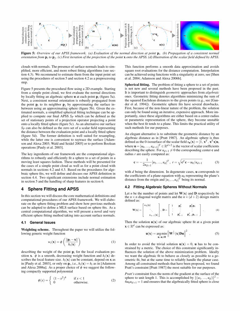
Figure 5: Overview of our APSS framework. (a) Evaluation of the normal direction at point pi. (b) Propagation of a consistent normalorientation from pi to p j. (c) First iteration of the projection of the point x onto the APSS. (d) Illustration of the scalar field defined by APSS.

clouds with normals. The presence of surface normals leads to sim-plified, more efficient, and more robust fitting algorithms (see sec-tion 4.3). We recommend to estimate them from the input point setusing the procedures of section 5 and section 4.2 as a preprocessingstep.

Figure 5 presents the procedural flow using a 2D example. Startingfrom a simple point cloud, we first evaluate the normal directionsby locally fitting an algebraic sphere u at each point pi (figure 5a).Next, a consistent normal orientation is robustly propagated fromthe point pi to its neighbor p j by approximating the surface in-between using an approximating sphere (figure 5b). Given the es-timated normals, a simplified spherical fitting technique can be ap-plied to compute our final APSS SP which can be defined as theset of stationary points of a projection operator projecting a pointonto a locally fitted sphere (figure 5c). As an alternative our surfaceSP can also be defined as the zero set of a scalar field representingthe distance between the evaluation point and a locally fitted sphere(figure 5d). The former definition is well suited for resampling,while the latter one is convenient to raytrace the surface [Adam-son and Alexa 2003; Wald and Seidel 2005] or to perform Booleanoperations [Pauly et al. 2003].

The key ingredients of our framework are the computational algo-rithms to robustly and efficiently fit a sphere to a set of points in amoving least squares fashion. These methods will be presented forthe cases of a simple point cloud as well as for a point cloud withnormals in sections 4.2 and 4.3. Based on the procedures for alge-braic sphere fits, we will define and discuss our APSS definition insection 4.4. Two significant extensions include normal estimationin section 5 and the handling of sharp features in section 6.

4 Sphere Fitting and APSSIn this section we will discuss the core mathematical definitions andcomputational procedures of our APSS framework. We will elabo-rate on the sphere fitting problem and show how previous methodscan be adapted to define a MLS surface based on sphere fits. As acentral computational algorithm, we will present a novel and veryefficient sphere fitting method taking into account surface normals.

4.1 General Issues

Weighting scheme. Throughout the paper we will utilize the fol-lowing generic weight function

wi(x) = φ

(‖pi −x‖

hi(x)

)(1)

describing the weight of the point pi for the local evaluation po-sition x. φ is a smooth, decreasing weight function and hi(x) de-scribes the local feature size. hi(x) can be constant, depend on x asin [Pauly et al. 2003], or only on pi, i.e., hi(x) = hi as in [Adamsonand Alexa 2006a]. As a proper choice of φ we suggest the follow-ing compactly supported polynomial

φ(x) ={

(1− x2)4 if x < 10 otherwise. (2)

This function performs a smooth data approximation and avoidssquare root evaluations for the distance computation. Interpolationcan be achieved using functions with a singularity at zero, see [Shenet al. 2004; Adamson and Alexa 2006b].

Spherical fitting. The problem of fitting a sphere to a set of pointsis not new and several methods have been proposed in the past.It is important to distinguish geometric approaches from algebraicones. Geometric fitting denotes algorithms minimizing the sum ofthe squared Euclidean distances to the given points (e.g., see [Gan-der et al. 1994]). Geometric sphere fits have several drawbacks.First, because of the non-linear nature of the problem, the solutioncan only be found using an iterative, expensive approach. More im-portantly, since these algorithms are either based on a center-radiusor parametric representation of the sphere, they become unstablewhen the best fit tends to a plane. This limits the practical utility ofsuch methods for our purposes.

An elegant alternative is to substitute the geometric distance by analgebraic distance as in [Pratt 1987]. An algebraic sphere is thusdefined as the 0-isosurface of the scalar field su(x) = [1, xT , xT x]u,where u = [u0, ..., ud+1]T ∈Rd+2 is the vector of scalar coefficientsdescribing the sphere. For ud+1 6= 0 the corresponding center c andradius r are easily computed as:

c =− 12ud+1

[u1, ..., ud ]T , r =√

cT c−u0/ud+1 (3)

with d being the dimension. In degenerate cases, u corresponds tothe coefficients of a plane equation with u0 representing the plane’sdistance from the origin and [u1, ..,ud ]T being its normal.

4.2 Fitting Algebraic Spheres Without Normals

Let n be the number of points and let W(x) and D respectively bethe n×n diagonal weight matrix and the n× (d +2) design matrixdefined as:

W(x) =

w0(x)

. . .wn−1(x)

, D =

1 pT0 pT

0 p0......

...1 pT

n−1 pTn−1pn−1

. (4)

Then the solution u(x) of our algebraic sphere fit at a given pointx ∈ Rd can be expressed as:

u(x) = argminu, u6=0

∥∥∥W12 (x)Du

∥∥∥2. (5)

In order to avoid the trivial solution u(x) = 0, u has to be con-strained by a metric. The choice of this constraint significantly in-fluences the solution of the above minimization problem. Ideallywe want the algebraic fit to behave as closely as possible to a ge-ometric fit, but at the same time to reliably handle the planar case.Among all constrained methods that have been proposed, we foundPratt’s constraint [Pratt 1987] the most suitable for our purposes.

Pratt’s constraint fixes the norm of the gradient at the surface of thesphere to unit length 1. This is accomplished by ‖(u1, ..., ud)‖2 −4u0ud+1 = 1 and ensures that the algebraically fitted sphere is close

to the least squares Euclidean best fit, i.e., the geometric fit (seealso figure 6). By rewriting the above constraint in matrix formuT Cu = 1, the solution u(x) of our minimization problem yields asthe eigenvector of the smallest positive eigenvalue of the followinggeneralized eigenproblem:

DT W(x)Du(x) = λCu(x), with C =

0 0 · · · 0 −20 1 0...

. . ....

0 1 0−2 0 · · · 0 0

. (6)

Note that this method is only used to estimate the missing normalsof input point sets. An efficient algorithm for running the APSS inthe presence of normals will be derived in the following section.

4.3 Fitting Spheres to Points with Normals

While the problem of fitting a sphere to points has been investigatedextensively, there exists to our knowledge no method to take spe-cific advantage of normal constraints at the sample positions. Wederive a very efficient algorithm by adding the following derivativeconstraints ∇su(pi) = ni to our minimization problem (5). Notethat, by definition, it holds that ‖ni‖= 1, which constrains both di-rection and magnitude of the normal vector. This is especially im-portant to force the algebraic distance to be close to the Euclideandistance for points close to the surface of the sphere. Furthermore,the normal constraints lead to the following standard linear systemof equations that can be solved very efficiently:

W12 (x)Du = W

12 (x)b (7)

where

W(x) =

. . .

wi(x)βwi(x)

. . .

βwi(x). . .

, D =

.

.

.

.

.

.

.

.

.

1 pTi pT

i pi

0 eT0 2eT

0 pi...

.

.

.

.

.

.

0 eTd−1 2eT

d−1pi...

.

.

.

.

.

.

, b =

.

.

.

0eT

0 ni...

eTd−1ni

.

.

.

. (8)

Here, {ek} denote the unit basis vectors of our coordinate system.The scalar β allows us to weight the normal constraints. We willdiscuss the proper choice of this parameter subsequently. We solvethis equation using the pseudo-inverse method, i.e.:

u(x) = A−1(x)b(x) (9)

where both the (d+2)×(d+2) weighted covariance matrix A(x)=DT W(x)D and the vector b(x) = DT W(x)b can be computed di-rectly and efficiently by weighted sums of the point coefficients.

The issue of affine invariance of this method deserves some furtherdiscussion. While the method’s invariance under translations androtations is trivial, the mix of constraints representing algebraic dis-tances and distances between unit vectors makes it slightly sensitiveto scale. A simple and practical solution is to choose a large valuefor β , e.g. β = 106h(x)2 where h(x) = ∑i wi(x)hi(x)

∑i wi(x) is a smooth func-tion describing the local neighborhood size (1). This effectivelyassigns very high importance to the derivative constraints, which,prescribed at given positions and with a fixed norm, are sufficientto fit a spherical isosurface to the data. The positional constraintsstill specify the actual isovalue. Not only does this choice leave thefitting invariant under scale, but it also makes it more stable, muchless prone to oscillations (figure 3b) and less sensitive to outliers.This choice does not unbalance the relative importance of the posi-tions and normals of the samples because the derivative constraintsdepend on both the sample positions and normals.

Figure 6: The Euclidean distance (green cone) versus an algebraicdistance (orange paraboloid) to the 2D yellow circle. Pratt’s nor-malization makes these two surfaces tangent to each other at thegiven circle.

4.4 Algebraic Point Set Surfaces

Implicit surface definition. The previous sections provide all in-gredients to define an MLS surface based on sphere fits. Our APSSSP, approximating or interpolating the point set P = {pi ∈ Rd},yields as the zero set of the implicit scalar field f (x) representingthe algebraic distance between the evaluation point x and the fittedsphere u(x). This field is illustrated in figure 5d:

f (x) = su(x)(x) =[1, xT , xT x

]u(x) = 0 . (10)

If needed the actual Euclidean distance to the fitted algebraic sur-face can be computed easily by its conversion to an explicit form.

Gradient. This implicit definition allows us to conveniently com-pute the gradient of the scalar field which is needed to obtain thesurface normal or to perform an orthogonal projection. We com-pute the gradient ∇ f (x) as follows:

∇ f (x) = [1, xT , xT x]∇u(x) +

0 eT0 2eT

0 x...

......

0 eTd−1 2eT

d−1x

u(x) . (11)

The value of the gradient ∇u(x) =(

du(x)dx0

, du(x)dx1

, . . .)

depends on the fit-ting method. With the Pratt’s constraint, the derivatives can be com-puted as the plane fit with covariance analysis case (see [Alexa andAdamson 2004]). With our normal constraint, the derivatives canbe directly computed from equation (9):

du(x)dxk

= A−1(x)(− dA(x)

dxku(x)+

db(x)dxk

). (12)

Curvature. The implicit definition can be used to compute higherorder differential surface operators, such as curvature. In prac-tice, however, the evaluation of the shape matrix involves expensivecomputations. Our sphere fit provides an elegant estimate of themean curvature readily available by the radius of the fitted sphere(3). This estimate of the mean curvature is in general very accurate,except when two pieces of a surface are too close to each other.In this case the samples of the second surface can lead to an over-estimation of the curvature. Note that in such cases our normalconstraint fitting method still reconstructs a correct surface withoutoscillations (figure 3b). The sign of this inexpensive mean curva-ture estimate is determined by the sign of un+1 and can be utilizedfor a variety of operations, such as accessibility shading shown infigure 1.

Projection procedure. Since the presented APSS surface defini-tion is based on a standard MLS, all the projection operators for theplane case can easily be adapted to our setting by simply replac-ing the planar projection by a spherical projection. Following theconcept of almost orthogonal projections in [Alexa and Adamson2004] we recommend the following procedure as a practical recipeto implement APSS: Given a current point x, we iteratively definea series of points qi, such that qi+1 is the orthogonal projection ofx onto the algebraic sphere defined by u(qi). Starting with q0 = x,

the projection of x onto the surface is asymptotically q∞. The re-cursion stops when the displacement is lower than a given precisionthreshold. This procedure is depicted in figure 5c.

Including surface normals into the definition comes with additionalsignificant advantages. First, it makes the scalar field f (x) to beconsistently signed according to the inside/outside relative positionof x. Such consistent orientation is fundamental to perform booleanoperations or collision detections for instance. Furthermore, point-normals provide a first order approximation of the underlying sur-face and thus allow for smaller neighborhoods at the same accuracy.Tighter neighborhoods do not only increase stability, but also accel-erate the processing. To this end, we recommend the normal esti-mation procedure described in the following section to preprocessa raw input point cloud.

5 Estimation of Surface Normals

Our method for normal estimation draws upon the same principle asthe one proposed by Hoppe et al. [1992]. The novelties include thenormal direction estimation and new heuristics for the propagationof the normal orientation. We will focus on these two issues.

5.1 Normal Direction

To estimate the normal direction ni of a point pi of our input pointset, we essentially take the gradient direction at pi of our MLS sur-face definition described in the previous section, i.e., ni = ∇ f (pi).Here, the computation of the algebraic sphere is based on the eigen-vector method described in section 4.2. In practice, we can approx-imate the accurate gradient direction of the scalar field f (appendix)with the gradient of the fitted algebraic sphere u(pi), i.e.:

ni ≈ ∇su(pi)(pi) =

0 eT0 2eT

0 pi

......

...0 eT

d−1 2eTd−1pi

u(pi) . (13)

This step is illustrated in figure 5a. Although the sphere normalcan differ from the actual surface normal, the above simplificationis reasonable, because the approximation is usually very close tothe accurate surface normal for points evaluated close to an inputsample. In practice, we never experienced any problems with it.

During this step we also store for each point a confidence valueµi that depends on the sanity of the neighborhood used to estimatethe normal direction. We take the normalized residual value, i.e.,µi = λ/∑

d+1k=0 |λk| where λk are the d + 2 eigenvalues and λ is the

smallest positive one. Similar confidence estimates were used be-fore by several authors (e.g. [Pauly et al. 2004]) in combination

p ph

i

pj

mc

pi

pj

(a) (b)

Figure 7: (a) Illustration of the BSP neighborhood of a point pi:each neighbor defines a halfspace limiting the neighborhood. Theblue points correspond to a naive kNN with k = 6. (b) Illustrationof Ψi j. The angle between the gradient of the fitted sphere (greenarrows) and the normal direction (shown in red here) serves as ameasure for the reliability of the normal propagation.

(a)

(b) (c) (f)

(d) (e)

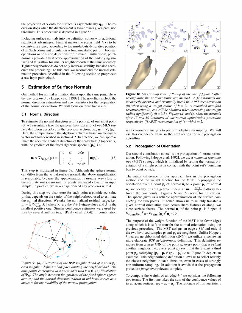
Figure 8: (a) Closeup view of the tip of the ear of figure 2 afterrecomputing the normals using our method. A few normals areincorrectly oriented and eventually break the APSS reconstruction(b) when using a weight radius of h = 2. A smoothed manifoldreconstruction (c) can still be obtained when increasing the weightradius significantly (h = 3.5). Figures (d) and (e) show the normalsafter 15 and 30 iterations of our normal optimization procedurerespectively. (f) APSS reconstruction of (e) with h = 2.

with covariance analysis to perform adaptive resampling. We willuse this confidence value in the next section for our propagationalgorithm.

5.2 Propagation of Orientation

Our second contribution concerns the propagation of normal orien-tation. Following [Hoppe et al. 1992], we use a minimum spanningtree (MST) strategy which is initialized by setting the normal ori-entation of a single point in contact with the point set’s boundingbox to point outside.

The major difference of our approach lies in the propagationmethod and the weight function for the MST. To propagate theorientation from a point pi of normal ni to a point p j of normaln j we locally fit an algebraic sphere at m = pi+p j

2 halfway be-tween the two points. Figures 3c and 5b serve for illustration.The sphere gives us a reliable approximation of the surface con-necting the two points. It hence allows us to reliably transfer agiven normal orientation even across sharp features or along twoclose surface sheets. The normal n j of the point p j is flipped if∇su(m)(pi)T ni ·∇su(m)(p j)T n j < 0.

The purpose of the weight function of the MST is to favor edgesalong which it is safe to transfer the normal orientation using theprevious procedure. The MST assigns an edge i- j if and only ifthe two involved samples pi and p j are neighbors. Unlike Hoppe’sk-nearest neighborhood definition (kNN), we utilize a somewhatmore elaborate BSP neighborhood definition. This definition re-moves from a large kNN of the point pi every point that is behindanother neighbor, i.e., every point p j such that there exist a thirdpoint ph satisfying (pi −ph)T (p j −ph) < 0. Figure 7a depicts anexample. This neighborhood definition allows us to select reliablythe closest neighbors in each direction, even in cases of stronglynon-uniform sampling. In addition it avoids that the propagationprocedure jumps over relevant samples.

To compute the weight of an edge i- j we consider the followingtwo terms: The first one takes the sum of the confidence values ofits adjacent vertices: µi j = µi +µ j. The rationale of this heuristic is

to push the samples with the lowest confidence values to the bottom(i.e. the leaves) of the tree. The second term Ψi j is computed byfirst fitting a sphere at the center m of the edge and by quantifyingthe difference between the gradient of the sphere and the estimatednormal direction. Ψi j is defined as the dot product between the twovectors, i.e., Ψi j = 1− (|∇su(m)(pi)T ni|+ |∇su(m)(p j)T n j|)/2. Asillustrated in figure 7b, this confirms our intuition that the propa-gation of normal directions is less obvious when the two vectorsdeviate strongly. We finally weight each edge i- j by a weightedsum of µi j and Ψi j, an empirical choice being 8µi j +Ψi j.

For some rare difficult cases, we propose to use the actual normalsto further optimize the normals with low confidence. This is ac-complished by using our stable spherical fitting method from sec-tion 4.3. For the fit, we weight each normal constraint according toits respective confidence value. This ensures that samples of higherconfidence have increased importance for the fit. To further opti-mize accuracy, we process the samples starting with the ones havingthe highest average confidence of their neighborhood. Our normalestimation procedure is depicted figure 8.

6 Sharp Features

In this section we present a new approach to handle sharp featuressuch as creases, corners, borders or peaks. We will explain it in thecontext of APSS, but the discussed techniques can easily be usedwith any PSS definition. Our approach combines the local CSGrules proposed in [Fleishman et al. 2005] with a precomputed par-tial classification, and we present extensions for the robust handlingof borders and peaks. During the actual projection of a point x ontothe surface, we first group the selected neighbors by tag values.Samples without tags are assigned to all groups. Then, the APSS isexecuted for each group and the actual point is projected onto eachalgebraic sphere. Next, we detect for each pair of groups whetherthe sharp crease they form originates from a boolean intersection orfrom a union and apply the corresponding CSG rule. We refer to[Fleishman et al. 2005] for the details of this last step, and focus onthe novel aspects of our approach.

6.1 Tagging a Point Cloud

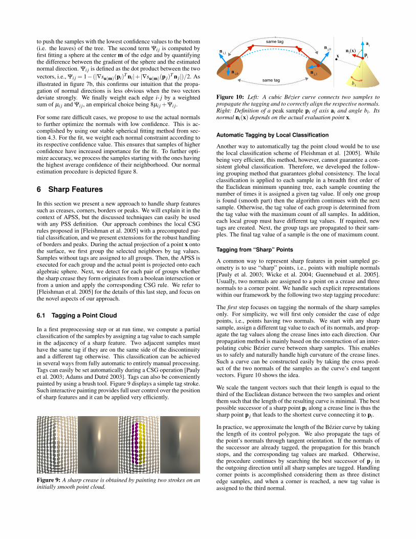
In a first preprocessing step or at run time, we compute a partialclassification of the samples by assigning a tag value to each samplein the adjacency of a sharp feature. Two adjacent samples musthave the same tag if they are on the same side of the discontinuityand a different tag otherwise. This classification can be achievedin several ways from fully automatic to entirely manual processing.Tags can easily be set automatically during a CSG operation [Paulyet al. 2003; Adams and Dutre 2003]. Tags can also be convenientlypainted by using a brush tool. Figure 9 displays a simple tag stroke.Such interactive painting provides full user control over the positionof sharp features and it can be applied very efficiently.

Figure 9: A sharp crease is obtained by painting two strokes on aninitially smooth point cloud.

a

pi

b i

x

i

n (x)i

same tag

same tagn j,0

n j,1n i,0

n i,1

Figure 10: Left: A cubic Bezier curve connects two samples topropagate the tagging and to correctly align the respective normals.Right: Definition of a peak sample pi of axis ai and angle bi. Itsnormal ni(x) depends on the actual evaluation point x.

Automatic Tagging by Local Classification

Another way to automatically tag the point cloud would be to usethe local classification scheme of Fleishman et al. [2005]. Whilebeing very efficient, this method, however, cannot guarantee a con-sistent global classification. Therefore, we developed the follow-ing grouping method that guarantees global consistency. The localclassification is applied to each sample in a breadth first order ofthe Euclidean minimum spanning tree, each sample counting thenumber of times it is assigned a given tag value. If only one groupis found (smooth part) then the algorithm continues with the nextsample. Otherwise, the tag value of each group is determined fromthe tag value with the maximum count of all samples. In addition,each local group must have different tag values. If required, newtags are created. Next, the group tags are propagated to their sam-ples. The final tag value of a sample is the one of maximum count.

Tagging from “Sharp” Points

A common way to represent sharp features in point sampled ge-ometry is to use “sharp” points, i.e., points with multiple normals[Pauly et al. 2003; Wicke et al. 2004; Guennebaud et al. 2005].Usually, two normals are assigned to a point on a crease and threenormals to a corner point. We handle such explicit representationswithin our framework by the following two step tagging procedure:

The first step focuses on tagging the normals of the sharp samplesonly. For simplicity, we will first only consider the case of edgepoints, i.e., points having two normals. We start with any sharpsample, assign a different tag value to each of its normals, and prop-agate the tag values along the crease lines into each direction. Ourpropagation method is mainly based on the construction of an inter-polating cubic Bezier curve between sharp samples. This enablesus to safely and naturally handle high curvature of the crease lines.Such a curve can be constructed easily by taking the cross prod-uct of the two normals of the samples as the curve’s end tangentvectors. Figure 10 shows the idea.

We scale the tangent vectors such that their length is equal to thethird of the Euclidean distance between the two samples and orientthem such that the length of the resulting curve is minimal. The bestpossible successor of a sharp point pi along a crease line is thus thesharp point p j that leads to the shortest curve connecting it to pi.

In practice, we approximate the length of the Bezier curve by takingthe length of its control polygon. We also propagate the tags ofthe point’s normals through tangent orientation. If the normals ofthe successor are already tagged, the propagation for this branchstops, and the corresponding tag values are marked. Otherwise,the procedure continues by searching the best successor of p j inthe outgoing direction until all sharp samples are tagged. Handlingcorner points is accomplished considering them as three distinctedge samples, and when a corner is reached, a new tag value isassigned to the third normal.

(b)(a)

Figure 11: (a) Illustration of boundaries handled using “clippingsamples” and an interpolatory weight function. (b) Illustration ofpeaks handled without any treatment (left part) and with our special“peak” samples (right part).

The second step involves a propagation of the tag values to the sam-ples close to a sharp edge, i.e., where distance is defined by the ac-tual weighting scheme. Tagging only the samples close to a sharpcrease specifically enables us to deal with non-closed creases as infigure 9. If pi is a smooth point and p j its closest sharp point havinga non-zero intersection of influence radii, the tag value of pi yieldsas the tag value of the normal of p j defining the plane closest to pi.A result of this procedure is depicted in figure 1-right.

6.2 Extensions

Object boundaries can be treated using “clipping samples”. A setof clipping points defines a surface that is only used to clip anothersurface. In order to simplify both the representation and the usercontrol, we place such clipping samples at the positions of bound-ary samples. Similar to the above notion of sharp points it is suffi-cient to add a clipping normal to each sample at the desired bound-ary. A clipping normal is set orthogonal to the desired boundarycurve and should be tangent to the surface. Figure 11a illustratesthe concept. Obviously, clipping samples may also be tagged todefine boundary curves with discontinuities. Finally, the evaluationof the surface or the projection onto the surface only requires a mi-nor additional modification. Clipping samples are always treated inseparate groups and the reconstructed clipping surface is only usedto clip the actual surface by a local intersection operation. Auto-matic detection of boundaries in a point cloud can easily be doneby analyzing the neighborhood of each sample, such as in [Guen-nebaud et al. 2005].

Handling “peak” discontinuities also deserves some special at-tention. We propose to explicitly represent a peak by a point piequipped with an axis ai and an angle bi, i.e., by a cone, as illus-trated in figure 10. During the local fitting step, we take as thenormal ni(x) of such a peak sample the normal of the cone in thedirection of the evaluation point x. ni(x) thus yields as the unitvector ai rotated by angle π

2 − bi and axis ai × (x− pi). We alsoguarantee that the surface will be C0 at the peak by attaching aninterpolating weight function to peak samples. The results in figure11b demonstrate that our method produces high quality peaks.

Figure 12: Illustration of the sharpness control, from left to right:α = 0, α = 0.15, α = 0.5, α = 1.

The sharpness control of a crease feature by a user parameter caneasily be added to our concept. To this end we insert all samplesinto all groups but assign a lower weight to a sample when insertedinto a group with a tag different from its own one. We define aglobal or local parameter α ∈ [0,1] which modulates the weight ofthese samples. For α = 0 we obtain a fully sharp feature, for α = 1the feature is completely smoothed since all groups are weightedidentically. Values in-between permit a continuous transition fromsmooth to sharp (figure 12).

7 Results

7.1 Implementation and Performance

In addition to a software implementation, we accelerated the pro-jection operator described in section 4.4 on a GPU. Our implemen-tation relies on standard GPGPU techniques and computes all thesteps of the projection, including neighbor queries, the fitting stepand the orthogonal projection, in a single shader. We use gridsof linked lists as spatial acceleration structures. Our implementa-tion performs about 45 million projection iterations per second ona NVidia GeForce 8800-GTS for APSS, compared to 60 millionfor SPSS. As detailed in table 1, our APSS projection operator con-verges about two times faster than SPSS making APSS overall about1.5 times faster for the same precision. As we can see, a single it-eration is usually sufficient to obtain a reasonable precision, whileSPSS achieves a similar accuracy only after 2 to 3 iterations.

# iter. 1 2 3 4 5 6APSS 2.01e-4 3.72e-5 1.9e-5 1.53e-5 1.38e-5 1.28e-5SPSS 1.94e-3 4.62e-4 1.67e-4 7.53e-5 3.95e-5 2.32e-5

Table 1: Comparison of the convergence of APSS and SPSS. Thevalues indicate the relative average precision obtained after thegiven number of iterations for a typical set of models.

The results of MLS surfaces depend significantly on the weightfunctions. Although we tried to find best settings for each method,other weight functions could lead to other, potentially better results.In particular, we performed all our comparisons on uniform pointclouds using the weight function described in section 4.1 with aconstant weight radius hi(x) = h ·r where h is an intuitive scale fac-tor and r is the average point spacing.Moreover, our IMLS imple-mentation corresponds to the “simple” definition given in [Kolluri2005]:

f (x) = ∑wi(x)(x−pi)T ni

∑wi(x)= 0. (14)

In order to conveniently handle arbitrary point clouds we suggest touse hi(x) = h ·ri where ri is the local point spacing that is computedas the distance to the farthest neighbor of the point pi using ourBSP neighborhood definition. An open source library of our APSSframework is available at: http://graphics.ethz.ch/apss.

7.2 Analysis of Quality and Stability

Approximation and interpolation qualityFigure 4 compares the ability of our spherical MLS to perform tightapproximation and convex interpolation. For interpolation we usedφ(x) = log(x)4 for both APSS and IMLS and φ(x) = 1/x2 for thetwo others. The values of h used for this figure are summarized inthe following table (interpol./approx.):

SPSS HPSS IMLS APSS3.35 / na na / na 1.95 / 1.95 1.95 / 3.25

(a) (b) (d)(c)

Figure 13: (a) Initial dense chameleon model from which 4k samples have been uniformly picked (depicted with red dots). This low sampledmodel is reconstructed using APSS (h = 1.9) (b), SPSS (h = 1.8) (c) and IMLS (h = 2.6) (d).

Stability for Low Sampling RatesOne of the central advantages of our spherical MLS is its abilityto robustly handle very low sampling densities as illustrated in fig-ure 13. The figure compares the approximation quality of a uni-formly sampled 4K chameleon model for APSS, SPSS and IMLS.We can clearly see the superior quality of APSS. We computed thetexture colors from the original dense model. In order to quantita-tively evaluate the robustness under low sampling and the approx-imation quality, we iteratively created a sequence of subsampledpoint sets P0,P1, . . . by first decomposing the current point set Piinto disjunctive point pairs using a minimum weight perfect match-ing (see [Waschbusch et al. 2004] for a similar scheme). A subse-quent projection of the pair centers onto the actual PSS Si yields areduced point set Pi+1. The graph in figure 14 shows the relativeaverage distance of the initial point set P0 onto various PSS Si asa function of the number of samples. Note that the graph is givenon a logarithmic scale. The results demonstrate that the APSS isabout three times more precise than the planar MLS variants. Fur-thermore, the planar versions break already at much higher sam-pling rates (crosses in the diagram), while APSS allows for stablefit at very low sampling rate. The instability of Levin’s operator ismainly due to the polynomial projection which requires a relativelylarge and consistent neighborhood. The distribution of the error isshown for an example in figure 15.Stability for Changes of WeightsFigure 16 compares the stability of APSS versus SPSS as a functionof the size of the weight radii. We utilized a higher order genusmodel with very fine structures and a low sampling density. As canbe seen SPSS exhibits undesired smoothing already at small radiiand breaks quickly at larger sizes. In this example, APSS alwaysdelivers the expected result, and the surface stays reasonably closeto original data even for large radii.

7.3 Unwanted Extra Zeros

Our spherical fitting algorithm can exhibit an increased sensitivitywith respect to unwanted stationary points away from the surface.We refer to [Adamson and Alexa 2006a] for a discussion of the pla-nar fit. With spheres, such extra zeros can specially occur close to

153k 76k 38k 19k 9.5k 4.7k 1.4k 1.2k 597 299 150 75 38 191E-6

1E-5

1E-4

1E-3

1E-2

1E-1

APSS

SPSS

IMLS

Levin's

# pts

Ave

rage

dis

plac

emen

t

Figure 14: Logarithmically scaled graph of the average projectionerror for the Chinese Dragon model.

the boundary of the surface definition domain D when for instancea small set of points yields a small and stable sphere that lies en-tirely inside D . D is the union of the balls centered at the samplepositions pi and having the radius of the weight function (h ·ri). Wehandle such spurious extra zeros by limiting the extent of D , i.e. byboth reducing the ball radii and removing regions in which fewerthan a given number (e.g., 4) of samples have non-zero weights.We found that this solution is working well in practice, but admitthat in-depth theoretical analysis is needed as part of future work.

8 Conclusion and Future WorkWe have demonstrated that the planar fit utilized in conventionalPSS implementations can successfully be replaced by spherical fits.Our sphere fit MLS has numerous significant advantages and over-comes some of the intrinsic limitations of planar MLS. In particular,we obtain an increased stability for low sampling rates, a tighter fit,a better approximation quality, robustness, and for-free mean cur-vature estimation. Fast numerical procedures and efficient imple-mentations allow for the processing of very complex, high-qualitymodels and make APSS as fast as simple MLS. Extensions of themethod handle discontinuities of various kinds. An apparent nat-ural extension of the method would be to employ ellipsoids, espe-cially for highly anisotropic objects, such as cylinders. Algebraicellipsoidal fits, however, do not naturally degenerate to planes. Incontrast, our method handles such objects correctly, as can be seenon the saddle configuration of figure 1-right.

Future work comprises applications of the representation in inter-active modeling. We believe that the method is well-suited for de-formations of point sampled geometry where the surface normalscould be estimated directly from the gradient operator. Another im-portant issue is the theoretical analysis of both unwanted extra zerosand the sampling requirements for our setting. Finally, we want toexplore its extension to non-manifold geometry as well as realtimeray-tracing of dynamic APSS.

(a) (b) (c)0% 0.6%

Figure 15: Chinese Dragon model (150 K) approximated withAPSS (a) and color-coded magnitude of the displacement betweenthe input samples and a low resolution model (19 K) using APSS(b) and SPSS (c).

Figure 16: A sparsely sampled point model (19 K) handled withAPSS (top row) and with SPSS (botton row) using different sizes ofthe weight radii: 1.6, 4, 8.

Acknowledgments

This work was supported in part by the ERCIM “Alain Bensoussan”Fellowship Programme. We would like to thank all reviewers fortheir insightful comments and discussions of the method, as wellas Mario Botsch and Ronny Peikert for proof reading the paper.The models of figures 15 and 16 are provided courtesy of INRIAand SensAble by the AIM@SHAPE Shape Repository. The tree offigure 1 is provided courtesy of Vincent Forest.

References

ADAMS, B., AND DUTRE, P. 2003. Interactive boolean opera-tions on surfel-bounded solids. ACM Transactions on Graphics(SIGGRAPH 2003 Proceedings) 22, 3, 651–656.

ADAMSON, A., AND ALEXA, M. 2003. Approximating and inter-secting surfaces from points. In Proceedings of the EurographicsSymposium on Geometry Processing 2003, 230–239.

ADAMSON, A., AND ALEXA, M. 2004. Approximating bounded,non-orientable surfaces from points. In Proceedings of ShapeModeling International 2004, IEEE Computer Society.

ADAMSON, A., AND ALEXA, M. 2006. Anisotropic point setsurfaces. In Afrigraph ’06: Proceedings of the 4th internationalconference on Computer graphics, virtual reality, visualisationand interaction in Africa, ACM Press, 7–13.

ADAMSON, A., AND ALEXA, M. 2006. Point-sampled cell com-plexes. ACM Transactions on Graphics (SIGGRAPH 2003 Pro-ceedings) 25, 3, 671–680.

ALEXA, M., AND ADAMSON, A. 2004. On normals and projectionoperators for surfaces defined by point sets. In Proceedings of theEurographics Symposium on Point-Based Graphics, 149–156.

ALEXA, M., AND ADAMSON, A. 2006. Interpolatory point setsurfaces - convexity and hermite data. Submitted paper.

ALEXA, M., BEHR, J., COHEN-OR, D., FLEISHMAN, S., LEVIN,D., AND SILVA, C. T. 2003. Computing and rendering point setsurfaces. IEEE Transactions on Computer Graphics and Visual-ization 9, 1, 3–15.

AMENTA, N., AND KIL, Y. 2004. Defining point-set surfaces.ACM Transactions on Graphics (SIGGRAPH 2004 Proceedings)23, 3, 264–270.

AMENTA, N., AND KIL, Y. 2004. The domain of a point set sur-face. In Proceedings of the Eurographics Symposium on Point-Based Graphics 2004, 139–147.

BOISSONNAT, J.-D., AND CAZALS, F. 2000. Smooth shape recon-struction via natural neighbor interpolation of distance functions.In Proceedings of the 16th Annual Symposium on ComputationalGeometry, ACM Press, 223–232.

DEY, T. K., AND SUN, J. 2005. An adaptive MLS surface for re-construction with guarantees. In Proceedings of the Eurograph-ics Symposium on Geometry Processing 2005, 43–52.

DEY, T. K., GOSWAMI, S., AND SUN, J. 2005. Extremal sur-face based projections converge and reconstruct with isotopy.manuscript.

FLEISHMAN, S., COHEN-OR, D., AND SILVA, C. T. 2005. Robustmoving least-squares fitting with sharp features. ACM Transac-tions on Graphics (SIGGRAPH 2005 Proceedings) 24, 3, 544–552.

GANDER, W., GOLUB, G. H., AND STREBEL, R. 1994. Least-squares fitting of circles and ellipses. BIT Numerical Mathemat-ics 34, 4, 558–578.

GUENNEBAUD, G., BARTHE, L., AND PAULIN, M. 2005. Interpo-latory refinement for real-time processing of point-based geom-etry. Computer Graphics Forum (Proceedings of Eurographics2005) 24, 3, 657–666.

HOPPE, H., DEROSE, T., DUCHAMP, T., MCDONALD, J., ANDSTUETZLE, W. 1992. Surface reconstruction from unorganizedpoints. In Proc. of ACM SIGGRAPH ’92, ACM Press, 71–78.

KAZHDAN, M., BOLITHO, M., AND HOPPE, H. 2006. Poissonsurface reconstruction. In Proceedings of the Eurographics Sym-posium on Geometry Processing 2006, 43–52.

KOLLURI, R. 2005. Provably good moving least squares. In ACM-SIAM Symposium on Discrete Algorithms, 1008–1018.

LEVIN, D. 2003. Mesh-independent surface interpolation. Geo-metric Modeling for Scientific Visualization, 181–187.

MITRA, N. J., NGUYEN, A., AND GUIBAS, L. 2004. Estimatingsurface normals in noisy point cloud data. International Journalof Computational Geometry and Applications 14, 4–5, 261–276.

OHTAKE, Y., BELYAEV, A., ALEXA, M., TURK, G., AND SEI-DEL, H.-P. 2003. Multi-level partition of unity implicits. ACMTransactions on Graphics (SIGGRAPH 2003 Proceedings) 22,3, 463–470.

PAULY, M., KEISER, R., KOBBELT, L. P., AND GROSS, M. 2003.Shape modeling with point-sampled geometry. ACM Transac-tions on Graphics (SIGGRAPH 2003 Proceedings) 22, 3.

PAULY, M., MITRA, N. J., AND GUIBAS, L. 2004. Uncertaintyand variability in point cloud surface data. In Proceedings of theEurographics Symposium on Point-Based Graphics, 77–84.

PRATT, V. 1987. Direct least-squares fitting of algebraic surfaces.In Proc. of ACM SIGGRAPH ’87, ACM Press, 145–152.

SHEN, C., O’BRIEN, J. F., AND SHEWCHUK, J. R. 2004. Inter-polating and approximating implicit surfaces from polygon soup.ACM Transactions on Graphics (SIGGRAPH 2004), 896–904.

WALD, I., AND SEIDEL, H.-P. 2005. Interactive ray tracing ofpoint based models. In Proceedings of the Eurographics Sympo-sium on Point Based Graphics 2005.

WASCHBUSCH, M., GROSS, M., EBERHARD, F., LAMBORAY,E., AND WURMLIN, S. 2004. Progressive compression of point-sampled models. In Proceedings of the Eurographics Symposiumon Point-Based Graphics 2004, 95–102.

WICKE, M., TESCHNER, M., AND GROSS, M. 2004. CSG treerendering of point-sampled objects. In Proceedings of PacificGraphics 2004, 160–168.