Allocation Policies in Blood Transfusion
Hossein Abouee-Mehrizi †, Opher Baron∗, Oded Berman∗, Vahid Sarhangian∗
†Department of Management Sciences, University of Waterloo, Waterloo, Ontario N2L 3G1, Canada
[email protected]∗Joseph L. Rotman School of Management, University of Toronto, Toronto, Ontario M5S 3E6, [email protected], [email protected], [email protected]
Red Blood Cell (RBC) transfusion is an integral part of many medical treatments and surgeries. Recently,
a growing body of research suggests a correlation between the age of transfused blood and adverse clinical
outcomes for its recipients. Therefore, there is a need for effective and practical inventory management
policies which could reduce the age of transfused RBC units without compromising their availability. In this
paper, we focus on policies which determine how RBC units are allocated to patients. We study a stylized
queueing model of a hospital blood bank and consider a family of threshold based allocation policies. We
characterize the sojourn time distribution of RBC units in inventory and calculate the distribution of the
age of transfused units, as well as the proportion of lost demand and outdates. Our analysis allows us to
capture the age-availability trade-off achieved under the threshold policy. In a numerical study, we explore
the factors affecting the performance of the threshold policy and investigate when it is more likely to be
effective in comparison to reducing the shelf-life. We find that when reducing the shelf-life has a high impact
on availability, the threshold policy is more effective. This is observed, in particular, for blood types with
lower demand, for smaller hospitals, and when a lower age of transfused RBCs is required. Furthermore,
using our analytical results together with models mapping the age of RBCs to the corresponding probability
of adverse medical outcomes, we examine the trade-off between availability and the health outcomes achieved
under the threshold policy. In particular, we demonstrate the importance of taking into account the entire
distribution of the age of transfused RBCs when evaluating the health outcomes of allocation policies.
Key words : Allocation policies; age-availability trade-off; perishable inventory systems; queues.
1. Introduction
1.1. Background and Motivation
Red Blood Cell (RBC) transfusion is an integral part of many medical treatments and surgeries;
in 2011, over 13 million units of voluntarily donated RBCs were transfused to patients across the
United States (NBCUS 2011). While advances in storage solutions led to an increase of RBCs
shelf-life from 35 to 42 days in the late 1970s, an extensive body of recent cohort studies (e.g.,
Koch et al. (2008), Eikelboom et al. (2010), Offner et al. (2002), Frank et al. (2013)) suggests
a range of moderate to strong correlation between receiving “older” blood and increased risk of
adverse medical outcomes such as infection, morbidity, and mortality. The results are however
1
Abouee-Mehrizi, Baron, Berman and Sarhangian: Allocation Policies in Blood Transfusion2
still inconclusive (Lelubre et al. 2009). It remains for undergoing randomized controlled clinical
trials such as ABLE (Lacroix 2011) to further clarify the relationship between the age of blood
and patient outcomes; a question which has been referred to as “the most critical issue facing
transfusion medicine” (Ness 2011).
It will take several years before the results of these clinical trials are available. Nevertheless, if
it turns out that there is indeed an association between receiving older blood and increased risk of
complications, the resulting increase in demand for fresher blood could have a significant impact
on the supply and availability of RBC units in blood banks and hospitals (Dzik et al. 2013, Sayers
and Centilli 2012). It is therefore of crucial importance to understand this impact and be ready
to adapt to new regulations on the shelf-life of RBCs. While the medical community works on
understanding the “storage lesion” and the efficacy of RBC transfusions, the operations research
community can contribute by exploring new inventory policies. A recent commentary (Sayers and
Centilli 2012) in the journal of Transfusion, specifically emphasizes the need for inventory and
supply chain management policies that could contribute to reducing the age of transfused RBC
units without compromising the adequacy of supply. Nevertheless, although there are a few papers
investigating the impact of shortening the shelf-life of blood (e.g., Fontaine et al. 2011, Blake et al.
2012), limited attention has been given to alternative inventory policies.
In this paper, we focus on the RBC allocation policy, i.e., the policy according to which the
RBC units are allocated to patients in the hospital. The impact of the allocation policy can be
intuitively understood by comparing two extreme policies namely the First-in, First-Out (FIFO)
and Last-In, First Out (LIFO) policies. Under the FIFO policy, which is the most commonly used
in practice (Dzik et al. 2013), always the oldest available unit is allocated to a new demand for
transfusion. While this favors availability by minimizing the number of outdated units, it clearly
results in a higher age of transfused units comparing to the LIFO policy which always allocates
the freshest unit available. This trade-off between the age and availability motivates the important
question of whether by adopting a different allocation policy, the age of transfused units can be
reduced to a desired level without significantly affecting the availability of units in the hospital.
We study a family of threshold based allocation policies previously introduced in the literature.
The policy was originally proposed by Haijema et al. (2007) in the context of platelet inventory
management, and was used to explore the “age–availability” trade–off for RBCs in a simulation
study by Atkinson et al. (2012). Under the threshold policy, the oldest RBC unit that is younger
than a given threshold is transfused, and if no such unit is available, the freshest available unit
Abouee-Mehrizi, Baron, Berman and Sarhangian: Allocation Policies in Blood Transfusion3
is allocated. To wit, the threshold policy includes both the FIFO and LIFO policies and aims to
capture the age-availability tradeoff by using a controlled combination of both policies.
The main goal of our analysis is to develop a better understanding of the performance and
benefits of the threshold policy as an important and practical family of allocation policies. While
previously proposed in the literature, the performance of the threshold policy under different
system parameters and its benefits over reducing the shelf-life under the FIFO policy are not well-
understood. Furthermore, previous studies only consider the average age of transfused RBC units.
However, since the relation between the age of blood and the probability of adverse outcomes could
potentially be nonlinear (see Pereira 2013 for potential relationship functions), understanding the
health benefit of allocation policies requires information on the resulting distribution of the age
of transfused units. The objectives of this study are thus to (i) evaluate the performance of the
threshold policy in terms of the resulting availability and distribution of the age of transfused RBC
units; (ii) asses its performance for different system parameters and in comparison to reducing the
shelf-life under the FIFO policy; and (iii) provide further insights on the age-availability trade-off
and design of allocation policies.
1.2. Analytical Framework, Contributions and Summary of Results
We study a stylized queueing model of a hospital blood bank by adopting the framework of Kaspi
and Perry (1983). In particular, we assume the following. Donors (supply) and demand for RBC
units arrive to the hospital according to independent Poisson processes. The supply side resem-
bles that of a hospital which locally collects blood from volunteers. Even though many hospitals
use ordering policies and receive deliveries of RBCs from regional suppliers, they still face high
variability in the size of deliveries. In general one expects a high variability on both the demand
and supply side, which supports the Poisson assumption. For instance, in Atkinson et al. (2012)
it is observed that the output of simulation is close to the empirical data when the coefficient of
variation (CV) of both donations and demand is set to 1.32. The assumption is also validated using
data from a regional blood center in Canada in Kopach et al. (2008). This assumption also implies
that donors donate one unit of RBC, and demand is also satisfied by one unit. The latter does
not always hold in reality as some patients may require multiple units of RBCs. While in practice
compatible blood types are sometimes substituted for one another, for tractability we assume that
the demand and supply for the inventory of each blood type is independent of other types. In
addition, in accordance with current practice, we assume that RBC units can be transfused up to a
Abouee-Mehrizi, Baron, Berman and Sarhangian: Allocation Policies in Blood Transfusion4
fixed number of days (currently 42) after donation and are discarded after this deadline. Finally, we
assume that unsatisfied demand is lost and the required RBC units are imported from an external
source, as is common in practice.
These assumptions allow us to model the blood bank as a queuing system operating under the
discipline corresponding to the allocation policy. Particularly, the oldest-blood-first and freshest-
blood-first policies translate to FIFO and LIFO queueing disciplines, respectively. Although styl-
ized, the model captures the main operational features of the system namely uncertainty in demand
and supply and the fixed shelf-life of RBC units. It also provides us with a framework to implement
allocation policies and study their outcomes.
This paper makes contributions to both queueing theory and blood inventory management lit-
eratures. On the theoretical end, we present the first exact analysis of the stochastic perishable
inventory system operating under the threshold policy. Our analysis are based on a two–stage
model of the system. In this model, fresh units arrive at Stage 1, but move to Stage 2 if their
sojourn time exceeds the threshold value. Demand is satisfied using the oldest unit from Stage 1.
If Stage 1 is empty, then the freshest unit in Stage 2 is allocated. As a result, Stage 1 is a FIFO
system with supply and demand processes identical to those of the original system, while Stage
2 is a LIFO system whose supply and demand processes are respectively driven by the outdate
and loss processes of Stage 1. The main complexity in the analysis of the threshold policy is that
the supply and demand processes of Stage 2 depend on the state of Stage 1. Consequently, direct
analysis of Stage 2 inventory without considering the dynamics of Stage 1 is not possible. Further,
the sojourn time of units in Stage 2 is bounded, as the shelf-life is finite. Our main contribution is
to develop a novel method to characterize the sojourn time of RBC units in Stage 2 inventory for
a given threshold value.
We first assume that units have infinite shelf-life in Stage 2 and characterize the sojourn time
of units under this assumption. The main idea behind our approach is to track a tagged unit in
Stage 2 and decompose its sojourn time into idle and busy periods of Stage 1 which operates under
the FIFO policy. Thus, the first part of our analysis is to characterize these idle and busy periods
by extending the results for the FIFO system. We then construct a sequence of modified Stage 2
systems in which the sojourn time of units is limited to a finite number of Stage 1 idle and busy
periods. We show that as the number of idle and busy periods considered asymptotically tends to
infinity, the sojourn time of units in these modified systems converges (in distribution) to that of
the units in the actual system. Finally, we employ the asymptotic analysis of the modified systems
Abouee-Mehrizi, Baron, Berman and Sarhangian: Allocation Policies in Blood Transfusion5
to obtain the performance measures of interest for the original system, i.e., the distribution of the
age of transfused RBC units and the proportion of outdates and lost demand.
On the application end, we provide several insights on the age–availability trade–off for RBCs.
Specifically, we provide insights on when the threshold policy is more likely to be effective and per-
form better than reducing the shelf-life under the FIFO policy. Our numerical study demonstrates
that the effectiveness of the threshold policy increases as the size of the hospital and the demand size
for individual blood types decreases. In contrast, for larger hospitals and blood types with higher
demand, or when a small reduction in the age of transfused RBCs is required, the performance of
the threshold policy is observed to be similar to that of simply reducing the shelf-life. Furthermore,
we incorporate the distribution of the age of transfused RBCs and demonstrate that the underlying
relationship between the age of transfused RBC units and the risk of adverse outcomes must be
considered when choosing an allocation policy. In particular, it is observed that when comparing
two different allocation policies under certain relationship functions, the one resulting in a lower
expected age of transfused units could lead to a higher probability of adverse outcomes. Finally,
our exact results on the trade–off between availability and the expected age of transfused RBCs
substantiate those based on the simulation study of Atkinson et al. (2012).
1.3. Related Literature
Analyzing perishable inventory systems using queueing theory goes back to Graves (1978, 1982)
and Nahmias (1980). The model considered in this paper was first introduced by Graves (1978) and
further studied in Kaspi and Perry (1983). They analyze the model under the FIFO discipline and
obtain performance measures of the system including the distribution of the time between outdates,
and that of the number of units in the system. Many papers have since considered variations and
extensions of the so called stochastic perishable inventory problem. Examples include the problem
with renewal supply (Kaspi and Perry 1984), quality inspections (Perry 1999), and batch demand
and donations (Goh et al. 1993). A direct application of this model to RBC inventory management
is also studied in Kopach et al. (2008). A common assumption among almost all these papers is
that the system operates under the FIFO policy. There are a few number of notable exceptions. In
Keilson and Seidmann (1990), the authors study the LIFO policy. Parlar et al. (2011) also consider
the LIFO policy and compare its performance with that of FIFO in a profit maximization setting.
Goh et al. (1993) provide approximate analysis for a two-stage system where units arrive at Stage
1, but move to Stage 2 after passing an age threshold. Each stage has an independent demand
Abouee-Mehrizi, Baron, Berman and Sarhangian: Allocation Policies in Blood Transfusion6
stream. The issuing policy within each stage is FIFO, however, demand for Stage 2 can be satisfied
using Stage 1 inventory in case of a shortage. In contrast, our system has a single demand stream
that is satisfied from Stage 1 as long as there are units available. If Stage 1 is empty, demand is
fulfilled from Stage 2 when possible. Also, the issuing policy within Stage 1 is FIFO, but demand
is satisfied from Stage 2 in a LIFO manner. While in this case Stage 1 behaves similar to a regular
FIFO system, the analysis of Stage 2 is much more involved and requires a different approach.
Our work relates to an extensive body of literature on perishable inventory systems; see Nahmias
(2011), Baron (2011) and Karaesmen et al. (2011) for comprehensive reviews and Piersikalla (2004)
for applications in blood supply chain management. A closely related area is the study of allocation
or issuing policies in periodic inventory systems with perishable products. Pierskalla and Roach
(1972) consider the problem for a finite-horizon periodic system in which inventory is categorized
based on age levels. At the beginning of a period, the demand and supply for each category is
observed and a decision for assigning inventory to demand is made. Under the assumption that
the demand for any age level can be satisfied by the same or fresher categories, the optimality of
the FIFO policy in minimizing the total lost demand and outdates is established. It is also shown
that the FIFO policy minimizes the cumulative stockouts for all periods when excess demand
is backlogged. The results are proved for deterministic demand and supply, and their extension
to the stochastic case is discussed. Haijema et al. (2007) study inventory management of blood
platelets (shelf-life of 5-7 days) with two demand streams; “young” and “any”. For the first stream
younger platelets are highly preferred while the second stream can be satisfied using platelets of
any age. They implement the same threshold policy considered in this paper and use simulation
and Markov Decision Processes to develop near optimal order-up-to replenishment policies. In a
profit maximization setting Deniz et al. (2010) consider a product with a lifetime of two periods
and study joint replenishment-issuing decisions.
Finally, there are a few simulation studies in the medical literature directly related to our appli-
cation. Atkinson et al. (2012) develop a simulation model based on data from Stanford University
Medical Center and investigate the trade–off between the expected age of transfused units and
availability of units in the hospital. They observe that by adopting a policy with threshold equal
to 14 days, the hospital can reduce the average age of transfused blood by 10 to 20 days while
only increasing the fraction of lost demand by 0.5%. Blake et al. (2012) use a simulation model
to asses the impact of shorter shelf-life on the blood supply chain of Hema-Quebec. They find
that a shelf-life of 28 or 21 is feasible, but will have a higher impact on smaller hospitals. A shelf
Abouee-Mehrizi, Baron, Berman and Sarhangian: Allocation Policies in Blood Transfusion7
life of 14 or less is observed to result in excessive increases to outdates and emergency orders for
both the suppliers and hospitals of all size. They also find that high outdates and lost demand are
mainly related to rarer blood types. In another simulation study, Fontaine et al. (2011) investigate
the impact of reducing the shelf-life for Stanford University Medical Center. They observe a high
impact on both availability and outdates in case of reducing the shelf-life to 21 or less.
1.4. Organization of the Paper
We start with a formal description of our stylized queueing system and its performance measures
pertaining to the age and availability of transfused RBCs. In Section 3, we study two important
members of the family of threshold policies; namely the FIFO and LIFO policies. Before presenting
our main results in Section 5, we give some theoretical results for the FIFO policy in Section 4
required for our analysis of the threshold policy. Section 6 contains the results of our numerical
study. Finally, in Section 7 we present our concluding remarks and a discussion of future research.
Proof of Theorems 1 and 2 are given in the Appendix. The proof of all other results can be found
in the Online Appendix.
2. Model Description
In this section we describe the model and formally introduce the performance measures of interest.
Donated RBC units (hereinafter referred to as units) arrive at the hospital blood bank according
to a Poisson process with intensity λ. It is assumed that units are “fresh”, i.e., have age zero upon
arrival to the inventory. However, the analysis can be easily extended to the case where all units
are delayed for some constant time, e.g. for tests, before arriving at the inventory. Demand for
RBC transfusions occur according to an independent Poisson process with intensity µ. Shelf-life
of units in the inventory is equal to a constant γ. Demand occurring while the inventory level is
at zero is lost. Otherwise, if there are available units in the inventory then one is allocated to the
demand according to the policy in effect.
It is convenient to view the system as an M/M/1 +Ds queue in which donated units are the
arrivals and each service completion corresponds to a patient receiving a transfusion. The queue
has arrival rate λ, service rate µ, and its service discipline coincides with the allocation policy of
the system. In addition, units have a deterministic patience until the end of service (the +Ds in
the Kendall notation) equal to γ, i.e., abandon the system if their sojourn time exceeds γ.
Abouee-Mehrizi, Baron, Berman and Sarhangian: Allocation Policies in Blood Transfusion8
Consider the system operating under some allocation policy denoted by π, and let Sπ denote
the random variable associated with the steady-state sojourn time of units in inventory (or equiv-
alently in the corresponding queueing system). Observe that Sπ has a probability mass at γ and
a continuous density on (0, γ). For outdated units we have Sπ = γ, while for each transfused unit
Sπ ∈ (0, γ) is equal to the age of the unit at the time of transfusion.
We study the outdate probability qπ, and the cumulative distribution function (cdf) of the
random variable associated with the age of transfused units Aπ. Observe that both performance
measures can be expressed in terms of the random variable Sπ. The outdate probability is
qπ = P (Sπ = γ), (1)
and the cdf of Aπ is given by
Aπ(x) =
P (Sπ ≤ x|Sπ <γ) = P (Sπ ≤ x)/(1− qπ), 0≤ x< γ,1, x≥ γ. (2)
Another performance measure is the probability of a demand being lost `π which directly corre-
sponds to the availability of units in the hospital. As discussed in Parlar et al. (2011), a simple
conservation law relates this measure to the outdate probability. Under any policy π, as long as
the steady-state limits exist, we have
λ (1− qπ) = µ (1− `π) . (3)
It is clear from (3) that loss and outdate probability can both be used as measures of availabil-
ity when comparing policies. In particular, minimizing the outdate probability is equivalent to
minimizing the loss probability and vice versa.
We close this section by mentioning that, throughout the paper, whenever we refer to the Laplace
transform (LT) of a random variable we mean the LT of its probability density function (pdf) or
equivalently the Laplace-Stieltjes transform (LST) of its cdf.
3. Review of the FIFO and LIFO Policies
The above model has been previously studied in the literature under FIFO and LIFO policies.
Some of the methods used in the analysis, however, will be used in our evaluation of the threshold
policy. Furthermore, as previously mentioned, FIFO and LIFO belong to the family of threshold
policies. Therefore, we next review the relevant results and use them to obtain the performance
measures of interest under these policies.
Abouee-Mehrizi, Baron, Berman and Sarhangian: Allocation Policies in Blood Transfusion9
3.1. The LIFO Policy
The analysis of the LIFO policy is due to Keilson and Seidmann (1990) and Parlar et al. (2011),
who study the distribution of the sojourn time of units in the inventory, SL (where “L” is the
shorthand notation for LIFO). The analysis is based on the following observations, valid under the
LIFO policy. First, the sojourn time of a new unit arriving in inventory only depends on future
demand and unit arrivals. Second, for any unit with sojourn time less than γ, we know that all units
which arrived during the sojourn time of the unit also had sojourn times less than γ, and hence
were not outdated. It follows that SL = min(SL, γ), where SL is the random variable associated
with the sojourn time of units in inventory if they had infinite shelf-life. As discussed in Parlar
et al. (2011) since both the demand and supply are Poisson, SL has the same distribution as the
length of a busy period in an M/M/1 queue with arrival rate λ and service rate µ.
Given the above, the outdate probability is P (SL = γ) = P (SL ≥ γ). Parlar et al. (2011) also give
an expression for the LT of the truncated busy period SL, from which the LT of AL can be obtained.
The formula is however not computationally useful. In the following proposition we present all
performance measures of interest directly in terms of the cdf of the busy period B(x)≡ P (SL ≤ x),
which can be computed efficiently by numerically inverting its LT,
ˆ ∞0
e−θxB(x)dx=2µ
θ(λ+µ+ θ+
√(λ+µ+ θ)2− 4λµ
) ,(see, e.g., Gross et al. 2008, page 102). Note that when λ> µ, P (SL <∞) = (µ/λ)< 1, that is B(x)
is improper. However, since SL is bounded, for any positive λ and µ, P (SL <∞) = 1.
Proposition 1. Under the LIFO policy the outdate probability is
qL = 1−B(γ). (4)
Furthermore, the cdf of the age of transfused units is
AL(x) =
B(x)/(1− qL), 0≤ x< γ,1, x≥ γ, (5)
and the expected age of transfused units is given by
E[AL] = γ−´ γ0B(y)dy
1− qL . (6)
Abouee-Mehrizi, Baron, Berman and Sarhangian: Allocation Policies in Blood Transfusion10
!
W (t)
t
Busy Period
IdlePeriodResidual Busy Period
Figure 1 A typical sample path of the process W
3.2. The FIFO Policy
The stochastic perishable inventory problem under the FIFO policy was first studied in Graves
(1978) and Kaspi and Perry (1983) and recently revisited in Parlar et al. (2011). The analysis is
based on the so called Virtual Outdating Process (VOP) W ≡ W (t); t≥ 0, which returns, as a
function of time, the remaining time until the next outdate if no new demands were to arrive. VOP
is useful since it is a (strong) Markov process and contains important information about the state
of the system. In particular, the age of the oldest unit in inventory at any time t≥ 0 is γ−W (t),
the event W (s)> γ implies no inventory at time s, and W (s−) = 0 indicates that a unit was
outdated at time s.
W has cadlag (right-continuous with left limits) sample paths with upward jumps. Jumps occur
either when the oldest unit is allocated to a demand (when 0 <W < γ, at Poisson rate µ) or is
outdated (when W hits zero). In both cases, jump sizes are equal to the inter-arrival time of units
to the inventory and hence exponentially distributed with rate λ. Figure 1 illustrates a sample
path of process W .
Kaspi and Perry (1983) show that W has the same distribution as the virtual waiting time
process of an M/M/1 +D queue with arrival rate µ and service rate λ, in which the idle periods
are deleted and customers do not join the system if they have to wait more than γ before starting
service (the +D in the Kendall notation). Using this observation they obtain the steady-state
distribution of W . Let f denote the steady-state pdf of W . We have (Parlar et al. 2011)
f(x) =
f(0)e−(λ−µ)x, 0<x< γ,
f(0)eµγ−λx, x≥ γ, (7)
Abouee-Mehrizi, Baron, Berman and Sarhangian: Allocation Policies in Blood Transfusion11
where
f(0) =
λ(λ−µ)
λ−µe−(λ−µ)γ , λ 6= µ,λ
1+λγ, λ= µ.
Having the steady-state distribution of W , we can obtain the required performance measures. Let
“F” be the shorthand notation for FIFO policy. The following proposition summarizes the results.
Proposition 2. Under the FIFO policy the outdate probability is
qF =
λ−µ
λ−µe−(λ−µ)γ , λ 6= µ,1
1+λγ, λ= µ.
(8)
Furthermore, the cdf of the age of transfused units is
AF (x) =
e−(λ−µ)(γ−x)−e−(λ−µ)γ
1−e−(λ−µ)γ , λ 6= µ,0≤ x< γ,x/γ, λ= µ,0≤ x< γ,1, x≥ γ,
(9)
and the expected age of transfused units is given by
E[AF ] =
(λ−µ)γ−(1−e−(λ−µ)γ)(λ−µ)(1−e−(λ−µ)γ)
, λ 6= µ,γ2, λ= µ.
(10)
The tractable form of the performance measures under the FIFO policy allows us to obtain
simple yet useful structural results presented in the following corollary without a proof.
Corollary 1. Under the FIFO policy:
1. For a fixed supply-to-demand ratio (λ/µ), both the outdate probability qF and loss probability `F
are strictly decreasing in µ.
2. For a fixed supply-to-demand ratio (λ/µ), as µ increases, the expected age of transfused units
E[AF ] increases for λ> µ and decreases for λ< µ.
3. The distribution of the age of transfused units AF (·) is strictly convex for λ> µ, strictly concave
for λ< µ and uniform for λ= µ.
We shall demonstrate and discuss some of these results in the numerical study of Section 6.
4. Additional Results for the FIFO Policy
Before turning to the analysis of the threshold policy we need some additional results for a FIFO
system in which units have a shelf-life T . Consider the queueing counterpart of the system. The
queue alternates between busy and idle periods. During a busy period, there are units available
in inventory while during an idle period, the inventory is empty. We also define the residual busy
period as the time interval between the epoch when a unit is outdated until the start of the next
Abouee-Mehrizi, Baron, Berman and Sarhangian: Allocation Policies in Blood Transfusion12
idle period. In what follows, we present the distribution of the number of units that are outdated
during a (residual) busy period as well as the LT of the length of the (residual) busy period given
the number of outdates. We also obtain the distribution of lost demand during an idle period as
well as the LT of the length of the idle period given the number of lost demand.
We prove the results using sample path analysis of the process W . First, following Kaspi and
Perry (1983), we define the stopping time
τ = inft≥ 0;W (t) = 0 or W (t)>T,
on W (0)> 0. We shall use the notation Px and Ex to denote conditional probability and expec-
tation given the initial value W (0) = x> 0. Let us define
gx(θ) ≡ Ex[e−θτ1W (τ)=0], (11)
hx(θ) ≡ Ex[e−θτ1W (τ)>T]. (12)
Then for x> T , gx(θ) = 0 and hx(θ) = 1. For each x∈ (0, T ] from Kaspi and Perry (1983) (see also
Cohen 1982, page 548), we have
gx(θ) =e−α1(θ)x(λ+α1(θ))e
−α2(θ)T − e−α2(θ)x(λ+α2(θ))e−α1(θ)T
(λ+α1(θ))e−α2(θ)T − (λ+α2(θ))e−α1(θ)T, (13)
hx(θ) =(e−α2(θ)x− e−α1(θ)x)(λ+α1(θ))(λ+α2(θ))
λ((λ+α1(θ))e−α2(θ)T − (λ+α1(θ))e−α1(θ)T ), (14)
where
α1(θ) = (θ+µ−λ+ ((λ+µ+ θ)2− 4λµ)1/2)/2,
α2(θ) = (θ+µ−λ− ((λ+µ+ θ)2− 4λµ)1/2)/2.
From this one can obtain, given the starting point x ∈ (0, T ], the probability that W hits zero
before upcrossing T , that is
Px(W (τ) = 0) = gx(0) =e−(µ−λ)x− (λ/µ)e−(µ−λ)T
1− (λ/µ)e−(µ−λ)T, (15)
and the probability of its complimentary event, i.e., that W upcrosses T before hitting zero,
Px(W (τ)>T ) = hx(0) = 1− gx(0) =1− e−(µ−λ)x
1− (λ/µ)e−(µ−λ)T. (16)
Next, consider W right after a jump caused by hitting zero. Let t= 0 be the time of the jump
and note that the starting point W (0)∈ (0,∞) is exponentially distributed with rate λ. Let
p≡ P (W (τ)>T ), g(θ)≡E[e−θτ |W (τ) = 0], h(θ)≡E[e−θτ |W (τ)>T ].
Abouee-Mehrizi, Baron, Berman and Sarhangian: Allocation Policies in Blood Transfusion13
Observe that p is the probability that W upcrosses T before hitting zero, g(θ) is the LT of the
time it takes for W to hit zero given that it happens before upcrossing T , and h(θ) is the LT of
the time it takes for W to upcross T given that it occurs before hitting zero.
Lemma 1. For λ 6= µ,
g(θ) =
(λe−α2(θ)T (1− e−(λ+α1(θ))T )−λe−α1(θ)T (1− e−(λ+α2(θ))T )
(λ+α1(θ))e−α2(θ)T − (λ+α2(θ))e−α1(θ)T
)/(1− p),
h(θ) =
(e−λT +
(λ+α1(θ))(1− e−(λ+α2(θ))T )− (λ+α2(θ))(1− e−(λ+α1(θ))T )
(λ+α1(θ))e−α2(θ)T − (λ+α2(θ))e−α1(θ)T
)/p,
and for λ= µ,
g(θ) =
(2λ(eTδ(θ)− 1)
θ(eTδ(θ)− 1) + 2λ(eTδ(θ)− 1) + (eTδ(θ) + 1)δ(θ)
)/(1− p),
h(θ) =
(2e(T/2)(θ+δ(θ))δ(θ)
θ(eTδ(θ)− 1) + 2λ(eTδ(θ)− 1) + (eTδ(θ) + 1)δ(θ)
)/p,
where δ(θ)≡√θ(θ+ 4λ) and
p=
e−λT + (1−e−λT )−(λ/µ)(1−e−µT )
1−(λ/µ)e−(µ−λ)T , λ 6= µ,
1/(1 +λT ), λ= µ.(17)
We proceed with the analysis of the residual busy period R. Let M be the number of outdates
during the residual busy period. Also, let r(θ) denote the LT of R, and let rm(θ) denote the LT of
R given M =m.
Proposition 3. The number of units that are outdated during the residual busy period is Geomet-
rically distributed with parameter p as given in (17), i.e.,
P (M =m) = (1− p)mp, (18)
for m≥ 0. Moreover, the LT of the length of the residual busy period given M =m is
rm(θ) = h(θ)(g(θ)
)m, (19)
and the LT of the length of the residual busy period is given by
r(θ) =ph(θ)
1− (1− p)g(θ). (20)
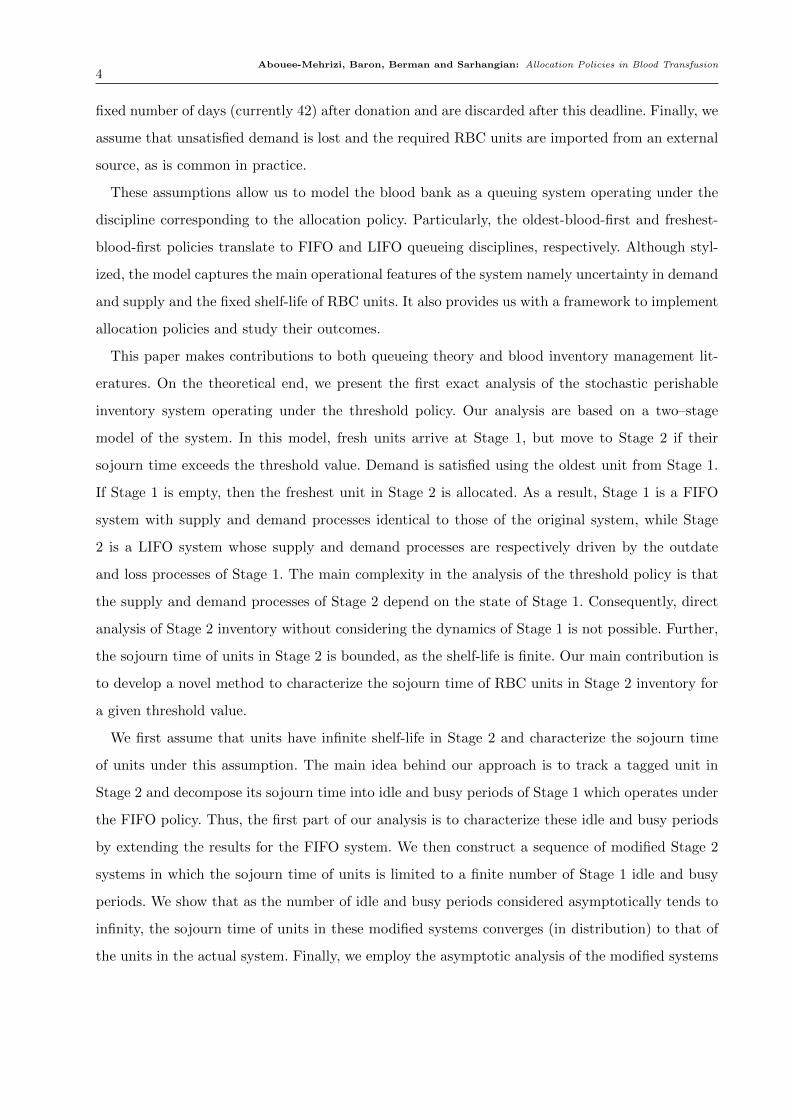
We next consider full busy periods (see Figure 1 for a realization). Note that the length of the
busy periods are i.i.d. random variables. Let N be the number outdates during a generic busy
period denoted by Z. Also, let z(θ) denote the LT of Z, and let zn(θ) denote the LT of Z given
N = n.
Abouee-Mehrizi, Baron, Berman and Sarhangian: Allocation Policies in Blood Transfusion14
Proposition 4. The distribution of the number of units that are outdated during a busy period is
given by
P (N = n) =
hT (0), n= 0,
gT (0)p(1− p)n−1, n > 0.(21)
Moreover, the LT of the length of the busy period given N = n is
zn(θ) =
hT (θ)
hT (0), n= 0,
gT (θ)
gT (0)h(θ) (g(θ))
n−1, n > 0,
(22)
and the length of the busy period has LT given by
z(θ) = hT (s) +ph(θ)gT (θ)
1− (1− p)g(θ). (23)
Finally, we consider the idle periods which are independent and exponentially distributed. Let
L be the number of lost demand during a generic idle period I. Also let i(θ) and il(θ) denote the
LT of I and the LT of I given L= l, respectively.
Proposition 5. Idle periods are exponentially distributed with parameter λ, that is
i(θ) =λ
λ+ θ. (24)
Moreover, the number of lost demand during an idle period is Geometrically distributed with param-
eter λ/(µ+λ), i.e.,
P (L= l) =
(µ
µ+λ
)l(λ
µ+λ
), (25)
and the length of the idle period given the number of lost demand L= l has an Erlang(l+ 1, λ+µ)
distribution, that is,
il(θ) =
(λ+µ
λ+µ+ θ
)l+1
. (26)
5. The Threshold Policy
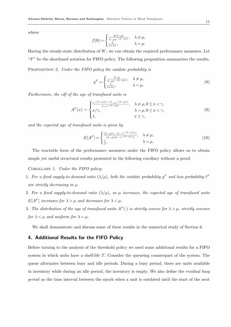
We analyze the threshold policy by considering a two-stage representation of the system operating
under a threshold policy with parameter T ∈ (0, γ). Figure 2 depicts this two-stage representation
of the system. Fresh units arrive at Stage 1 according to a Poisson process with rate λ and stay
there for a maximum of T time units after which they are transferred to Stage 2. Units remain in
Stage 2 for up to γ−T additional time units and are eventually outdated if their age exceeds the
shelf-life γ before they are allocated. Demand for Stage 1 inventory occurs according to a Poisson
process with rate µ and is satisfied according to a FIFO policy. If there are no units available in
Abouee-Mehrizi, Baron, Berman and Sarhangian: Allocation Policies in Blood Transfusion15
µ
••
••T
뵕
Stage 1(FIFO)
•
Stage 2(LIFO)
Figure 2 A two–stage representation of the system under the threshold policy
Stage 1, a unit from Stage 2 is allocated according to a LIFO policy. Demand occurring while there
are no units available is lost.
Let “T” be the shorthand notation for a threshold policy with parameter T , so that ST is the
random variable representing the steady-state sojourn time of units under a threshold policy with
parameter T . Let ST1 ∈ (0, T ] denote the random variable representing the steady-state sojourn
time of units in Stage 1. Also, for units which transfer to Stage 2, let ST2 ∈ (0, γ − T ] denote the
random variable representing their steady-state sojourn time in Stage 2. To simplify the notation
we omit the superscript T from ST1 and ST2 . Then,
ST = S11S1<T+ (T +S2)1S1=T. (27)
It is easy to see that Stage 1 is an independent system operating under the FIFO policy, in
which units have shelf-life T . Hence, given that a unit is allocated from Stage 1, its sojourn time
distribution is known through the analysis of Subsection 3.2. In particular, let q1, `1, A1(·) and
E[A1], respectively, denote the outdate probability, loss probability, cdf of the age of transfused
units, and the expected age of transfused units in a FIFO system where units have shelf-life T .
Then all these measures can be obtained from Proposition 2 by setting γ = T .
However, both demand and arrival processes of Stage 2 depend on the state of Stage 1. During
a busy period in Stage 1, demand is only satisfied from Stage 1 inventory but units may pass the
threshold age T and hence move to Stage 2. During an idle period in Stage 1, demand is satisfied
from Stage 2 inventory but there are no arrivals at Stage 2. To characterize the distribution of
S2 we first consider a system in which units have infinite shelf-life in Stage 2. Let S2 denote the
random variable representing the steady-state sojourn time of units in this system. Then since
the allocation policy in Stage 2 is LIFO, using similar arguments to those in Section 3.1, we have
S2 = min(S2, γ−T ).
Abouee-Mehrizi, Baron, Berman and Sarhangian: Allocation Policies in Blood Transfusion16
Note that a unit can arrive at Stage 2 during a busy period in Stage 1 and can be allocated
to a demand during one of the idle periods of Stage 1. In general, however, since the shelf-life is
infinite, to find the sojourn time of allocated units one needs to consider infinitely many such idle
periods. Note that S2 has an improper distribution whenever λq1 >µ`1, in which case P (S2 <∞) =
(µ`1)/(λq1). Our approach is based on analyzing a sequence of modified Stage 2 systems in which
each unit can only be allocated during a finite number k of Stage 1 idle periods, after its arrival
at Stage 2. Specifically, in the kth modified system a unit which is not allocated by the end of the
kth busy period after its arrival at Stage 2 is discarded. We denote the random variable associated
with the steady-state sojourn time of units in the kth modified system by S2,k and show that as k
tends to infinity, the distribution of S2,k converges to that of S2. By analyzing the more tractable
random variable S2,k, we are then able to obtain the LT of S2.
In the next subsection, we explain how the required performance measures under the threshold
policy can be obtained from the distribution of S2. In Subsection 5.2 we analyze the modified
systems and use them to obtain the LT of S2.
5.1. Obtaining the Performance Measures
We first examine the outdate probability. For a unit to be outdated it must first move to Stage 2
and then, assuming it has an infinite shelf life, spend more than γ − T in Stage 2. Note that q1
is the probability that a unit moves to Stage 2. Hence, the outdate probability of a policy with
threshold T is given by
qT = q1P (S2 ≥ γ−T ). (28)
To obtain the distribution of the age of transfused units AT , we condition on whether the unit
is allocated while in Stage 1 or 2. Denote these events by S1 and S2, respectively, and note that
P (S1) +P (S2) + qT = 1. First, clearly P (AT ≤ x|S1) =A1(x). Second, given that a unit is allocated
from Stage 2, we know that its age is greater than T , and hence for x≤ T we have P (AT ≤ x|S2) = 0.
For T < x< γ,
P (AT ≤ x|S2) = P (S2 ≤ x−T )/P (S2 <γ−T ).
Noting that
P (S1) =1− q11− qT , P (S2) =
q1P (S2 <γ−T )
1− qT ,
Abouee-Mehrizi, Baron, Berman and Sarhangian: Allocation Policies in Blood Transfusion17
R I2
...
... Zk
Uk0 U1
IkZ1I1
t
...
...
Tagged unit moves toStage 2
Z0
Figure 3 An illustration of random variables R,Ii,Zi,Uk on the time line
and combining the two cases we have
AT (x)≡ P (AT ≤ x) =
P (S1)A1(x), x < T,
P (S1) + q11−qT P (S2 ≤ x−T ), T ≤ x< γ,
1, x≥ γ.(29)
Finally, the expected age of transfused units E[AT ], can be computed using
E[AT ] = E[A1]P (S1) +(T +E[S2|S2 <γ−T ]
)P (S2),
where
E[S2|S2 <γ−T ] = γ−T −´ γ−T0
P (S2 ≤ x)dx
P (S2 <γ−T ).
For all the performance measures, P (S2 ≤ x) for x ≤ γ − T can be computed by numerically
inverting its LT, i.e., E[e−θS2 ]/θ, where E[e−θS2 ] will be given in Theorem 4 of Subsection 5.2.
5.2. Sojourn Time of Units in Stage 2
In this subsection, we obtain the LT of S2 by considering a sequence of modified systems. Before
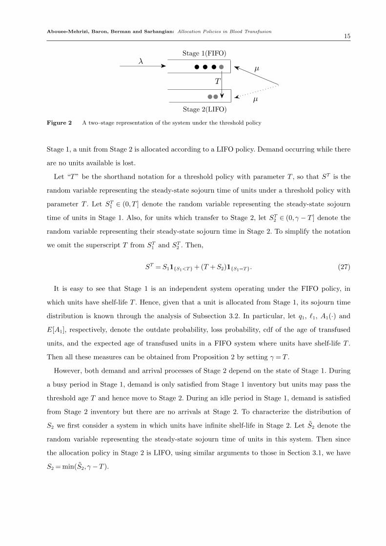
formalizing the approach we introduce some notation. Consider a tagged unit which has just arrived
at Stage 2. Let Zi, i≥ 0 and Ii, i≥ 1 denote, respectively, the length of the ith busy and idle period
in Stage 1 followed by the arrival of the tagged unit to Stage 2. Accordingly, Z0 corresponds
to the length of the busy period during which the unit arrives at Stage 2. Note that Ii; i ≥ 1and Zi; i≥ 0 are sequences of i.i.d. random variables having the same distribution as I and Z,
respectively. Thus, we have their LTs from Propositions 4 and 5, respectively. Furthermore, the
time interval between the epoch when the tagged unit moves to Stage 2 until the start of the first
idle period is a residual busy period R, the LT of which is given by Proposition 3. Let t= 0 be the
Abouee-Mehrizi, Baron, Berman and Sarhangian: Allocation Policies in Blood Transfusion18
instance the tagged unit moves to Stage 2 and let Uk, k ≥ 1, denote the time when the kth busy
period ends. That is, for k≥ 1,
Uk =R+k∑i=1
Ii +k∑i=1
Zi. (30)
Letting X0 =R and Xi = I +Z for i= 1,2, ..., and noting that Xi; i≥ 1 is an i.i.d sequence with
Xi > 0 for all i≥ 1, Uk, k ≥ 1 can be viewed as the arrival epochs of a delayed renewal process.
Figure 3 presents an illustration of the corresponding renewal process on the time line.
Now recall that S2,k is the sojourn time of units in the kth modified system in which a unit is
discarded if it is not allocated by the end of the kth busy period (or equivalently the beginning of
the (k+ 1)st idle period). Therefore, for a unit that is allocated by the end of the kth busy period
we have S2,k = S2, while for a unit that is still in the system by the end of the kth busy period we
have S2,k =Uk. Formally, for k≥ 1,
S2,k = S21S2<Uk+Uk1S2≥Uk. (31)
Theorem 1. Consider the sojourn time of units in Stage 2 assuming infinite shelf-life S2, and the
sojourn time of units in the kth modified system S2,k. We have
limk→∞
P (S2,k ≤ x) = P (S2 ≤ x), x∈ [0,∞),
limk→∞
E[e−θS2,k ] = E[e−θS2 ], θ > 0.
The theorem implies that for sufficiently large number of idle periods, the sojourn time distri-
bution of the units in the modified system becomes arbitrary close to that of units in the system
with infinite shelf-life. It also indicates that the LT of S2 can be obtained by first obtaining the
LT of S2,k and then letting k→∞. While the result is sufficient for our analysis, in the following
theorem we state a stronger convergence result for S2, i.e., the actual sojourn time of units in Stage
2. Recall that S2 = min(S2, γ−T ). Hence, similarly if we let
S2,k ≡min(S2,k, γ−T ), k≥ 1, (32)
denote the truncated sojourn time of units in the kth modified system, one would expect S2,k to
converge to S2 as k tends to infinity. Indeed, the following theorem establishes their almost sure
convergence.
Theorem 2. Consider S2 the actual sojourn time of units in Stage 2, and S2,k as defined in (32).
We have P (S2,k→ S2) = 1, that is the sequence of random variables S2,k converges to S2 with
probability 1.
Abouee-Mehrizi, Baron, Berman and Sarhangian: Allocation Policies in Blood Transfusion19
We now turn to the analysis of the modified systems. Consider the kth modified system. Note
that given the number of units that are in front of the tagged unit at the beginning of any idle
period, its remaining sojourn time is independent of the past. For the kth modified system, let
ϕkν,i(θ),1≤ i≤ k+1 denote the LT of the remaining sojourn time of the tagged unit at the beginning
of the ith idle period, given that it has ν units in front of it. Then, ϕkν,1(θ) is the LT of the remaining
sojourn time of the unit at the beginning of the first idle period, given that the number of units
moving to Stage 2 during the residual busy period is ν ≥ 0. Recall that M denotes the number of
outdates during the residual busy period and rν(θ) denotes the LT of the length of the residual
busy period given M = ν. Thus, we have
E[e−θS2,k ] =∞∑ν=0
P (M = ν)rν(θ)ϕkν,1(θ). (33)
We first express ϕkν,1(θ) for k≥ 1 in Theorem 3, then we use (33) to find the LT of S2,k. Finally, in
Theorem 4 we apply Theorem 1 to obtain the LT of S2.
The following lemma presents a recursive relation for ϕkν,i(θ), which can be used to obtain ϕkν,1(θ).
We consider the tagged unit at the beginning of the ith idle period given that it has ν ≥ 0 units
in front of it. We then condition on the number of demand arrivals during the idle period. By
considering two cases depending on whether the unit is allocated during the idle period or not, we
are able to relate the LT of the remaining sojourn time of the tagged unit at the beginning of the
ith idle period to that of the unit at the beginning of the (i+ 1)st idle period.
Lemma 2. For 1≤ i≤ k and ν ≥ 0 we have
ϕkν,i(θ) =ν∑l=0
∞∑n=0
P (L= l)P (N = n)il(θ)zn(θ)ϕkν+n−l,i+1(θ) +
(µ
µ+λ+ θ
)ν+1
. (34)
Note that by definition of ϕkν,i(θ) we have ϕkν,k+1(θ) = 1 for all ν ≥ 0. Thus, for a given k and
starting from i= k one can use Lemma 2 to recursively solve for ϕkν,1(θ). The next theorem expresses
ϕkν,1(θ) as a function of k. First, define
c1(θ)≡ h(θ)p
(µ
λ+µ+ θ
), c2(θ)≡ (1− p)g(θ)
(µ
λ+µ+ θ
), (35)
with g(θ), h(θ) and p given in Lemma 1, and let
ξi(θ)≡
hT (θ) + gT (θ)c1(θ)/ (1− c2(θ)) , i= 0,
ξ0(θ) + gT (θ)c1(θ)/ (1− c2(θ))2 , i= 1,
gT (θ)c1(θ) (c2(θ))i−2
/ (1− c2(θ))i+1, i≥ 2,
(36)
Abouee-Mehrizi, Baron, Berman and Sarhangian: Allocation Policies in Blood Transfusion20
βi(θ)≡c1(θ)/ (1− c2(θ)) , i= 0,
c1(θ) (c2(θ))i−1
/ (1− c2(θ))i+1, i≥ 1,
(37)
with hT (θ) and gT (θ) given in (15) and (16) respectively. Next, define the nested sum Yν(d) for
non-negative integers ν and d as
Yν(d)≡0∑
j0=0
ξj0(θ)1∑
j1=0
ξj1(θ)
2−j1∑j2=0
ξj2(θ)
3−j2−j1∑j3=0
ξj3(θ) · · ·
(d−1)−jd−2−···−j1∑jd−1=0
ξjd−1(θ)
(µ
λ+µ+ θ
)ν+1(ν+ 1
d− jd−1− · · ·− j1
), (38)
where we adopt the convention that any empty sum is equal to 0 and any empty product equal to
1. Note that d is the number of sums in Yν(d). For d= 0, Yν(d) has no sums, that is
Yν(0) =
(µ
λ+µ+ θ
)ν+1(ν+ 1
0
)=
(µ
λ+µ+ θ
)ν+1
,
and for d = 1 the expression only contains the first sum. Noting that the first sum simplifies to
ξ0(θ), we have
Yν(1) = ξ0(θ)
(µ
λ+µ+ θ
)ν+1(ν+ 1
1
).
Similarly, for d∈ 2,3, ..., (38) includes the first d sums.
Theorem 3. The LT of the remaining sojourn of a unit at the beginning of the first idle period in
the kth modified system, given it has ν ≥ 0 units in front of it ϕkν,1(θ) is given by
ϕkν,1(θ) =k−1∑i=0
Yν(i)(
1− (i(θ)z(θ))k−i)( λ
λ+µ+ θ
)i+(i(θ)z(θ)
)k. (39)
Using (33) we obtain E[e−θS2,k ] and let k→∞ to obtain the LT of S2. Define the nested sum
X(d,w) for positive integers d and w as
X(d,w)≡w∑
j1=0
ξj1(θ)
w+1−j1∑j2=0
ξj2(θ)
w+2−j2−j1∑j3=0
ξj3(θ) · · ·w+(d−2)−jd−2−···−j1∑
jd−1=0
ξjd−1(θ)βw+(d−1)−jd−1−···−j1(θ).
(40)
Note that X(d,w) contains the first d− 1 sums, such that X(1,w) = βw(θ) for all w ∈ 1,2, . . ..Moreover, X(d,w) satisfies the recursive relation given by
X(d,w) =w∑i=0
ξi(θ)X(d− 1,w+ 1− i),
for d ∈ 2,3, ..., which can be used to calculate X(i,1) for i ∈ 1,2, ..., as needed in Theorem 4
below.
Abouee-Mehrizi, Baron, Berman and Sarhangian: Allocation Policies in Blood Transfusion21
Theorem 4. The LT of S2 is given by
E[e−θS2 ] = β0(θ) + ξ0(θ)∞∑i=1
X(i,1)
(λ
λ+µ+ θ
)i.
6. Numerical Results and Observations
Let ϑ denote the age of units at the time of arrival to the inventory. Unless otherwise noted, similar
to Atkinson et al. (2012) we assume that it takes 2 days to test and process the units, i.e., we use
ϑ = 2 in the numerical examples. However, we shall specify the threshold T with respect to the
arrival of units to Stage 1. For instance, a threshold value of T = 4 implies that units move to Stage
2 after 6 days.
6.1. The Expected Age–Availability Trade-off
We start by investigating the trade-off between the expected age of transfused units and the loss
probability as a measure for availability. Since the age of blood is measured in days, we compute
the expected age of transfused units under a policy π using
EA(π) = ϑ+
γ∑n=1
n ·P (n− 1<Aπ <n),
where as mentioned earlier constant ϑ is the initial age of units at the time of arrival to the
inventory and γ = 42−ϑ is the maximum number of days units can be held in the inventory. Note
that here Aπ corresponds to the age of units at the time of transfusion with respect to their arrival
in inventory.
Figure 4 illustrates the tradeoff for µ= 15 (roughly the demand for A+ blood type at Stanford
University Medical Center) and different values of the supply-to-demand ratio. The qualitative
features of the trade-off curve we obtain are similar to those observed in Atkinson et al. (2012). The
shape of the trade-off curve depends on the supply-to-demand ratio: As the supply-to-demand ratio
increases, the tradeoff curve tends to a vertical line and the loss probability decreases. When the
ratio is 1.05, the curve is nearly vertical and the loss probability is very small (less than 0.01) for all
threshold values. On the other hand, as the ratio decreases the trade-off curve tends to a horizontal
line and the loss probability increases. When the ratio is 0.95 the curve is nearly horizontal and,
regardless of the policy, the loss probability is quite high (above 0.05). For supply-to-demand ratios
close to 1, a meaningful trade-off between the expected age and the loss probability is achieved. As
the threshold value decreases, we observe a large decrease in the expected age and a small increase
in the proportion of lost demand.
Abouee-Mehrizi, Baron, Berman and Sarhangian: Allocation Policies in Blood Transfusion22
0 0.01 0.02 0.03 0.04 0.05 0.060
5
10
15
20
25
30
35
40
Proportion of lost demand (imported units)
Ave
rage
age
oftr
ansf
use
dunit
s
λ/µ = 1.05
λ/µ = 1.02
λ/µ = 1.01
λ/µ = 1
λ/µ = 0.99
λ/µ = 0.97
λ/µ = 0.95
Figure 4 The trade-off between the expected age of transfused units and the loss probability. The six tick marks
on each curve from left to right correspond to threshold values of 40 (FIFO), 28, 14, 7, 4, and 0 (LIFO).
6.2. Performance of the Threshold Policy
Next, we take a closer look at the performance of the threshold policy when the supply-to-demand
ratio is close to 1. Tables 1 to 3 list the detailed performance of the threshold policy for systems with
large (µ= 15), medium (µ= 7), and small (µ= 2) demand sizes, respectively. The demand rates are
roughly equal to those for A+, B+ and AB+ blood types in Stanford University Medical Center.
For each demand rate, the performance of the policy is presented for different supply-to-demand
ratios and threshold values.
As we expect from (3), for each demand size, a higher supply-to-demand ratio results in a higher
outdate probability and a lower probability of loss. Moreover, the demand size plays an important
role in performance of the threshold policy. For a fixed supply-to-demand ratio, regardless of the
threshold value, we observe a better outcome in terms of the loss and outdate probability as the
demand rate increases. Furthermore, the range of outdate and loss probabilities among the policies
becomes smaller as the demand rate increases.
In Tables 1 to 3, for each policy, we also present the proportion of units which are transferred to
Stage 2. Note that this value is equal to the resulting outdate probability under the FIFO policy
if the shelf-life is reduced to the threshold value. Thus, by comparing this value to the outdate
probability of the corresponding threshold policy we are able to compare the performance of the
threshold policy with that of simply reducing the shelf-life to the threshold value.
Abouee-Mehrizi, Baron, Berman and Sarhangian: Allocation Policies in Blood Transfusion23
FIFO T = 28 T = 14 T = 7 T = 4 LIFO
λ/µ= 0.98
Prop. of units transferred to Stage 2 0 0.0000 0.0003 0.0028 0.0085 1
Prop. of units allocated from Stage 2 0 0.0000 0.0000 0.0000 0.0011 1
Outdate prob. for units transferred to Stage 2 - 1.0000 1.0000 0.9961 0.8726 0.0146
Outdate prob. 0.0000 0.0000 0.0003 0.0028 0.0075 0.0146
Loss prob. 0.0200 0.0200 0.0203 0.0227 0.0273 0.0343
Mean age of transfused units 5.9 5.9 5.6 4.9 4.1 3.7
λ/µ= 1.00
Prop. of units transferred to Stage 2 0 0.0024 0.0047 0.0094 0.0164 1
Prop. of units allocated from Stage 2 0 0.0000 0.0000 0.0000 0.0012 1
Outdate prob. for units transferred to Stage 2 - 1.0000 1.0000 0.9986 0.9293 0.0230
Outdate prob. 0.0017 0.0024 0.0047 0.0094 0.0152 0.0230
Loss prob. 0.0017 0.0024 0.0047 0.0094 0.0152 0.0230
Mean age of transfused units 22.5 16.5 9.5 6.0 4.5 3.7
λ/µ= 1.02
Prop. of units transferred to Stage 2 0 0.0196 0.0199 0.0223 0.0278 1
Prop. of units allocated from Stage 2 0 0.0000 0.0000 0.0000 0.0010 1
Outdate prob. for units transferred to Stage 2 - 1.0000 1.0000 0.9996 0.9638 0.0338
Outdate prob. 0.0196 0.0196 0.0199 0.0223 0.0268 0.0338
Loss prob. 0.0000 0.0000 0.0003 0.0027 0.0074 0.0145
Mean age of transfused units 39.1 27.1 13.4 7.1 4.9 3.7
Table 1 Performance of the threshold policy for µ= 15 and different values of supply-to-demand ratio
We observe that the demand size and the threshold value are two key factors in determining
the effectiveness of the threshold policy in comparison to reducing the shelf-life. Consider Table 1,
corresponding to the system with large demand. Even for small threshold values, almost all the
units transferred to Stage 2 are outdated (see outdate probability for units transferred to Stage
2), thereby effectively leading to the same outcome achieved when the shelf-life of units is reduced
to the threshold value. A similar outcome is achieved for large threshold values. For example, for
T = 28, regardless of the demand size, almost no units are allocated from Stage 2. However, when
the demand size is smaller (see Tables 2 and 3) and the threshold value is sufficiently small, a
considerable proportion of units are allocated from Stage 2. While the proportion is small enough to
keep the expected age of transfused units low, it results in a significantly smaller outdate probability
when compared to reducing the shelf-life. For instance, when λ = µ = 2 and T = 7 (see Table
3), 1.51% of units are allocated from Stage 2. The result is a lower outdate probability (5.24%)
compared to that of reducing the shelf-life to γ = 7 (6.67%).
Recalling that Stage 1 behaves like a FIFO system with shelf-life T , the above observation can
be explained in light of Corollary 1. Keeping the supply-to-demand ratio fixed, as the demand
decreases, the proportion of units transferred to Stage 2 and the proportion of demand directed to
Stage 2 increase. Reducing the threshold has a similar effect. The result is that a higher proportion
Abouee-Mehrizi, Baron, Berman and Sarhangian: Allocation Policies in Blood Transfusion24
of units are allocated from Stage 2 inventory, which in turn, increases the effectiveness of the
threshold policy over reducing the shelf-life in terms of availability.
It is important to note that the benefits of the threshold policy are less significant when the
impact of reducing the shelf-life on availability is smaller. Note that reducing the shelf-life results
in a larger increase in the outdate probability when the demand size is smaller. For example,
reducing the shelf-life to 14 increases the outdate probability from 0.0017 to 0.0047 (by 0.0030)
when λ= µ= 15, and from 0.0123 to 0.0345 (by 0.0222) when λ= µ= 2. Similarly, small reductions
in the shelf-life (e.g., to 28) have a small effect on the outdate probability regardless of the demand
size (although the effect is higher when the demand is smaller). These observations are inline with
those reported in the simulation study of Blake et al. (2012).
Alternatively, one could think of using a combination of the threshold policy and reduction of the
shelf-life. However, this is less likely to be effective. Consider a threshold policy with parameter T .
If we reduce the shelf-life γ, Stage 1 remains unchanged but the remaining shelf-life of units in Stage
2 (γ − T ) and hence the proportion of units allocated from this stage decreases. Therefore, when
compared to just using a threshold policy with parameter T , the expected age will be approximately
the same while the outdate probability will be higher.
In summary, a threshold policy results in almost the same expected age obtained if the shelf-
life is reduced to the threshold value. However, for a sufficiently small demand size and threshold
value, the threshold policy results in a lower outdate probability (and higher availability) when
compared to reducing the shelf-life. Thus, our results suggests that for blood types with high
demand or when a small decrease in the age of RBCs is required, the advantages of applying a
threshold policy comparing to reduction of the shelf-life are minimal. At the same time, we observe
a smaller effect on availability for such systems in case of a reduction in shelf-life. On the other
hand, for lower demand rates or when a larger reduction in the age of RBCs is required, as the
system becomes more vulnerable to the impact of reducing the shelf-life, a threshold policy is
expected to maintain a suitable utilization of Stage 2 inventory and thus be effective in improving
the availability. Extending this observation to hospital sizes, our model suggests a more significant
benefit in using the threshold policy for smaller hospitals where reducing the shelf-life has been
predicted to be more detrimental to the availability of RBC units (Blake et al. 2012); an observation
which is also evident from our results.
We close this subsection with a few important remarks on the comparison of the threshold policy
with shortening the shelf-life. First, although small threshold values may not seem plausible when
Abouee-Mehrizi, Baron, Berman and Sarhangian: Allocation Policies in Blood Transfusion25
FIFO T = 28 T = 14 T = 7 T = 4 LIFO
λ/µ= 0.98
Prop. of units transferred to Stage 2 0 0.0004 0.0033 0.0119 0.0260 1
Prop. of units allocated from Stage 2 0 0.0000 0.0000 0.0005 0.0073 1
Outdate prob. for units transferred to Stage 2 - 1.0000 1.0000 0.9554 0.7231 0.0250
Outdate prob. 0.0001 0.0004 0.0033 0.0113 0.0188 0.0250
Loss prob. 0.0201 0.0204 0.0232 0.0311 0.0384 0.0445
Mean age of transfused units 9.5 9.1 7.4 5.4 4.5 4.1
λ/µ= 1.00
Prop. of units transferred to Stage 2 0 0.0051 0.0101 0.0200 0.0345 1
Prop. of units allocated from Stage 2 0 0.0000 0.0000 0.0005 0.0074 1
Outdate prob. for units transferred to Stage 2 - 1.0000 1.0000 0.9732 0.7914 0.0337
Outdate prob. 0.0036 0.0051 0.0101 0.0195 0.0273 0.0337
Loss prob. 0.0036 0.0051 0.0101 0.0195 0.0273 0.0337
Mean age of transfused units 22.5 16.5 9.5 6.0 4.7 4.1
λ/µ= 1.02
Prop. of units transferred to Stage 2 0 0.0200 0.0227 0.0310 0.0446 1
Prop. of units allocated from Stage 2 0 0.0000 0.0000 0.0005 0.0070 1
Outdate prob. for units transferred to Stage 2 - 1.0000 1.0000 0.9845 0.8479 0.0440
Outdate prob. 0.0197 0.0200 0.0227 0.0305 0.0378 0.0440
Loss prob. 0.0001 0.0004 0.0032 0.0112 0.0185 0.0248
Mean age of transfused units 35.5 23.9 11.6 6.6 4.8 4.1
Table 2 Performance of the threshold policy for µ= 7 and different values of supply-to-demand ratio
FIFO T = 28 T = 14 T = 7 T = 4 LIFO
λ/µ= 0.98
Prop. of units transferred to Stage 2 0 0.0096 0.0260 0.0583 0.1034 1
Prop. of units allocated from Stage 2 0 0.0000 0.0004 0.0247 0.0555 1
Outdate prob. for units transferred to Stage 2 - 1.0000 0.9846 0.7498 0.4903 0.0543
Outdate prob. 0.0050 0.0096 0.0255 0.0437 0.0507 0.0543
Loss prob. 0.0249 0.0294 0.0450 0.0629 0.0697 0.0732
Mean age of transfused units 16.9 13.4 8.9 6.2 5.4 5.1
λ/µ= 1.00
Prop. of units transferred to Stage 2 0 0.0175 0.0345 0.0667 0.1111 1
Prop. of units allocated from Stage 2 0 0.0000 0.0004 0.0151 0.0550 1
Outdate prob. for units transferred to Stage 2 - 1.0000 0.9888 0.7857 0.5345 0.0630
Outdate prob. 0.0123 0.0175 0.0341 0.0524 0.0594 0.0630
Loss prob. 0.0123 0.0175 0.0341 0.0524 0.0594 0.0630
Mean age of transfused units 22.5 16.5 9.5 6.3 5.4 5.1
λ/µ= 1.02
Prop. of units transferred to Stage 2 0 0.0288 0.0446 0.0757 0.1192 1
Prop. of units allocated from Stage 2 0 0.0000 0.0004 0.0147 0.0540 1
Outdate prob. for units transferred to Stage 2 - 1.0000 0.9920 0.8181 0.5774 0.0724
Outdate prob. 0.0244 0.0288 0.0442 0.0619 0.0688 0.0724
Loss prob. 0.0049 0.0094 0.0251 0.0432 0.0502 0.0538
Mean age of transfused units 27.6 19.1 10.2 6.5 5.4 5.1
Table 3 Performance of the threshold policy for µ= 2 and different values of supply-to-demand ratio
Abouee-Mehrizi, Baron, Berman and Sarhangian: Allocation Policies in Blood Transfusion26
FIFO T = 4 T = 3 T = 2 LIFO
Prop. of units transferred to Stage 2 0 0.0278 0.0326 0.0424 1
Prop. of units allocated from Stage 2 0 0.0006 0.0026 0.0097 1
Outdate prob. for units transferred to Stage 2 - 0.9785 0.9225 0.7802 0.4956
Outdate prob. 0.0196 0.0272 0.0301 0.0331 0.0364
Loss prob. 0.0000 0.0078 0.0107 0.0138 0.0171
Mean age of transfused units 39.1 12.9 12.2 11.7 11.6
Table 4 Performance of the threshold policy for µ= 15, λ/µ= 1.02 and ϑ= 10
the age of units at the time of arrival to inventory is low, in some hospitals the age of units at
the time of receipt could be high (e.g., average 10.2 days reported for a hospital in Sayers and
Centilli (2012)), making small threshold values relevant. In Table 4, we report the performance
of the threshold policy with small threshold values for µ = 15 and λ/µ = 1.02 when ϑ = 10. We
observe that when the age of units at the time of receipt is relatively high, using a policy with
small thresholds could have significant benefits even when the demand size is large. Second, while
we observe a low utilization of Stage 2 inventory under the assumption of stationary supply and
demand, in practice, episodes of high demand or low supply could result in rapid consumption
of units in Stage 2 and hence further differentiate the threshold policy from reduction of the
shelf-life. Finally, as our numerical results suggest, the threshold policy provides similar or better
performance when compared to reducing the shelf-life and hence can be considered as a practical
alternative to it.
6.3. Going Beyond the Expected Age: Probability of Adverse Outcomes–Availability
Trade-off
So far, we have focused on the expected age of transfused units when assessing the outcome of
threshold policies. However, as mentioned in the introduction, the actual relationship between the
age of RBCs and their health outcomes is still under investigation. Thus, although in general the
proportion of units allocated from Stage 2 seems to be low and hence its effect on the average age
of transfused units insignificant, one should still be cautious about the age of transfused units from
Stage 2 as its health effects could be significant in the long term.
To investigate the factors that affect the distribution of the age of units transfused from Stage
2, we computed its cdf for different demand rates and supply-to-demand ratios. We observed that
while the supply-to-demand ratio has little effect on the shape of the distribution, the demand
size plays an important role. Figure 5 presents the cdf of the age of transfused units from Stage
2 for different supply-to-demand ratios and system sizes when T = 4. We observe that a higher
Abouee-Mehrizi, Baron, Berman and Sarhangian: Allocation Policies in Blood Transfusion27
0 5 10 15 20 25 30 35 400
0.2
0.4
0.6
0.8
1
Age of transfused blood
Cum
ilitiv
epro
bability
µ = 2, λ/µ = 0.98
µ = 7, λ/µ = 0.98
µ = 15, λ/µ = 0.98
0 5 10 15 20 25 30 35 400
0.2
0.4
0.6
0.8
1
Age of transfused blood
Cum
ilitiv
epro
bability
µ = 2, λ/µ = 1
µ = 7, λ/µ = 1
µ = 15, λ/µ = 1
0 5 10 15 20 25 30 35 400
0.2
0.4
0.6
0.8
1
Age of transfused blood
Cum
ilitiv
epro
bability
µ = 2, λ/µ = 1.02
µ = 7, λ/µ = 1.02
µ = 15, λ/µ = 1.02
Figure 5 Distribution of the age of transfused units from Stage 2 for threshold policy with T = 4
demand size is associated with a higher age of transfused units from Stage 2. On the other hand,
as the demand size decreases and hence a higher proportion of units are allocated from Stage 2,
the age of transfused units tend to be smaller. The figure is representative and we observe a similar
relationship for other threshold values not presented here.
Next, we examine the performance of the threshold policy under possible relationship functions
mapping the age of RBCs to the probability of adverse outcome after the transfusion. We consider
three hypothetical relationship functions suggested in Pereira (2013). The three models, which we
refer to as Model 1, 2 and 3 (see Figure 6), are based on the time course of storage induced defects,
reported in the medical literature. Model 3, for example, illustrates the case where units younger
than 14 days have no clinically detectable effect, but after 14 days the effect rapidly increases to
attain its maximum at 28 days. Given a relationship function J(·) and initial age of units ϑ, we
estimate the Average Probability of Adverse Outcomes (APAO) under an allocation policy π as
APAO(π) =
γ∑n=1
P (n− 1<Aπ <n)J(n+ϑ).
In figure 7, we illustrate the trade-off between APAO and proportion of lost demand achieved under
different allocation policies and supply-to-demand ratios for a system with µ = 2. As expected,
under the linear relationship function (Model 1) the trade-off curves look similar to those in Figure
4, i.e., the curves for the lost demand versus the expected age trade-off. The results are however
different for Models 2 and 3. We observe that a policy that results in a lower expected age could be
associated with higher probability of adverse outcomes. Under Model 3, for instance, for threshold
values 7, 4 and 0 (LIFO), both the proportion of loss demand and APAO are strictly higher
when compared to those for threshold value 14. The reason is that for these threshold values,
the relatively small proportion of units which are allocated from Stage 2 are associated with high
probability of adverse outcomes. On the contrary, when T = 14 almost all units are allocated from
Abouee-Mehrizi, Baron, Berman and Sarhangian: Allocation Policies in Blood Transfusion28
0 7 14 21 28 35 420
0.2
0.4
0.6
0.8
1
Age of transfused blood n
Pro
b.
ofad
vers
eou
tcom
esJ
(n)
J(n) = 0.024n
Model 1
0 7 14 21 28 35 420
0.2
0.4
0.6
0.8
1
Age of transfused blood n
Pro
b.
ofad
vers
eou
tcom
esJ
(n)
Model 2
J (n) = (1 + e−0.2(n−21) )−1
0 7 14 21 28 35 420
0.2
0.4
0.6
0.8
1
Age of transfused blood n
Pro
b.
ofad
vers
eou
tcom
esJ
(n)
Model 3
J (n) = (1 + e−(n−21) )−1
Figure 6 Three hypothetical models representing the relation between the age of transfused RBCs and probability
of adverse clinical outcomes.
0 0.01 0.02 0.03 0.04 0.05 0.06 0.07 0.08
0
0.1
0.2
0.3
0.4
0.5
0.6
0.7
Proportion of lost demand (imported units)
Ave
rage
pro
b.
ofadve
rse
outc
om
es
λ/µ = 0.98
λ/µ = 1
λ/µ = 1.02
Model 1
0 0.01 0.02 0.03 0.04 0.05 0.06 0.07 0.08
0
0.1
0.2
0.3
0.4
0.5
0.6
0.7
Proportion of lost demand (imported units)
Ave
rage
pro
b.
ofadve
rse
outc
om
es
λ/µ = 0.98
λ/µ = 1
λ/µ = 1.02
Model 2
0 0.01 0.02 0.03 0.04 0.05 0.06 0.07 0.08
0
0.1
0.2
0.3
0.4
0.5
0.6
0.7
Proportion of lost demand (imported units)
Ave
rage
pro
b.
ofadve
rse
outc
om
es
λ/µ = 0.98
λ/µ = 1
λ/µ = 1.02
Model 3
Figure 7 Trade-off between average probability of adverse outcomes and proportion of lost demand under three
different relationship models for µ= 2. The six tick marks on each curve from left to right correspond
to threshold values of 40 (FIFO), 28, 14, 7, 4, and 0 (LIFO).
Stage 1, resulting in a smaller APAO and probability of loss compared to lower threshold values.
We conclude that the underlying relationship between the age of RBCs and the corresponding
probability of adverse outcomes is an important factor that must be taken into account when
choosing an allocation policy. In particular, the expected age of transfused units may only be
a suitable measure for assessing the outcome of allocation policies, if the relation between the
probability of adverse outcomes and the age of RBCs is approximately linear.
Finally, while in the above trade-offs we used the loss probability as the measure for availability,
one should notice that a low loss probability, e.g., when the supply-to-demand ratio is high, could
be associated with a high outdate probability as reported in Tables 1 to 3. A high loss probability
translates into a high import rate of blood for hospitals. If the imported units are of higher age,
they could further increase the average probability of adverse outcomes. In this case the age of
imported units must be taken into account when assessing the outcome of allocation policies.
7. Conclusions
We study a stochastic perishable inventory system operating under a family of threshold allocation
policies. Our model captures the main operational features of a hospital blood bank. We provide
Abouee-Mehrizi, Baron, Berman and Sarhangian: Allocation Policies in Blood Transfusion29
an exact characterization of the sojourn time distribution of units for the threshold policy. This
allows us to observe the age-availability trade-off by computing the distribution of the age of
transfused units as well as the proportion of lost demand and outdates. Through a numerical
study, we provide insights on the benefits of the threshold policy and identify important factors
that should be considered when implementing any allocation policy. We observe that reducing the
shelf-life, specially in large amounts, has a higher impact on availability for smaller hospitals and
blood types with lower demand. We further find that in such cases the threshold policy is more
effective. Therefore, we recommend the threshold policy to be considered as a viable and practical
policy for reducing the age of transfused RBCs, specially where shortening the shelf-life is not
feasible. Moreover, our numerical study shows that the actual benefits of allocation policies depend
on the relationship between the entire distribution of the age of RBCs and the associated health
outcomes. Thus, design and implementation of any allocation policy must be in light of results
from the ongoing clinical trials.
Our study is the first to use an analytical approach in assessing the benefits of allocation policies
in the context of blood transfusion. Accordingly, future work should investigate the effects of
substitution of blood types, ordering policies, age of the units at the time of receipt by the hospital,
and batch demands on the age-availability trade-off. While we expect our insights to hold under
more general circumstances, empirical validation of the results would be of great value.
Finally, in this paper we focus on a simple and practical family of allocation policies. While
characterizing the optimal policy is of interest, both from the theoretical and practical perspectives,
it remains a challenging problem. Some initial work has been done by Sabouri et al. (2013).
Appendix A. Proof of Theorems 1 and 2.
Proof of Theorem 1. We first show that the cdf of S2,k converges to that of S2 for all x∈ [0,∞).
Then, the second part follows from the continuity theorem for Laplace transforms (see Feller 1971,
page 431). Let Aj denote the event that “the unit is allocated during the jth idle period” and let
Ak denote the event that “the unit is not allocated during any of the first k idle periods”. Note
that ∪kj=1Aj = S2 < Uk and Ak = S2 ≥ Uk. Now consider the cdf of S2,k. Using (31) we can
write
P (S2,k ≤ x) =k∑j=1
P (S2,k ≤ x|Aj)P (Aj) +P (S2,k ≤ x|Ak)P (Ak)
=k∑j=1
P (S2 ≤ x|Aj)P (Aj) +P (Uk ≤ x|Ak)P (Ak). (41)
Abouee-Mehrizi, Baron, Berman and Sarhangian: Allocation Policies in Blood Transfusion30
Letting k→∞ in (41), the last term on the RHS vanishes. To see this note that
limk→∞
P (Uk ≤ x|Ak)P (Ak) = limk→∞
P (Uk ≤ x, Ak)≤ limk→∞
P (Uk ≤ x) = 0,
where the last equality holds because Uk is the kth renewal epoch of a delayed renewal process.
Thus, for any x∈ [0,∞) we have
limk→∞
P (S2,k ≤ x) =∞∑j=1
P (S2 ≤ x|Aj)P (Aj) = P (S2 ≤ x).
Note that since x is finite the last equality follows even if the cdf of S2 is improper. Hence, the
proof is complete.
Proof of Theorem 2. To prove the theorem it is sufficient to show that for each ε > 0,∑∞k=1P (|S2,k−S2| ≥ ε)<∞. Then from the Borel-Cantelli Lemma we have P (|S2,k−S2| ≥ ε i.o.) =
0 (where i.o. stands for infinitely often) implying that P (S2,k→ S2) = 1 (see Billingsley 1995, page
70) as claimed. To this end, we consider the random variable S2 defined on a probability space
(Ω,F , P ) and decompose the sample space Ω for k≥ 1 as
C1,k ≡ ω ∈Ω; S2(ω)≤Uk(ω),
C2,k ≡ ω ∈Ω;γ−T ≤Uk(ω)< S2(ω),
C3,k ≡ ω ∈Ω;Uk(ω)<γ−T ≤ S2(ω),
C4,k ≡ ω ∈Ω;Uk(ω)< S2(ω)<γ−T,
such that ∪4i=1Ci,k = Ω for any k≥ 1. Note that since S2,k = min(S2,k, γ−T ), for any ω ∈C1,k∪C2,k
we have S2(ω) = S2,k(ω). Thus, for each ε > 0, |S2,k −S2| ≥ ε ⊆C3,k ∪C4,k, implying that for all
k≥ 1, P (|S2,k−S2| ≥ ε)≤ P (C3,k ∪C4,k). Therefore,
∞∑k=1
P (|S2,k−S2| ≥ ε) ≤∞∑k=1
P (C3,k ∪C4,k)≤∞∑k=1
P (Uk ≤ γ−T ).
It remains for us to show that∑∞
k=1P (Uk ≤ γ − T )<∞. Indeed, defining the stopping time σ =
infn≥ 1;Un >γ−T we have
∞∑k=1
P (Uk ≤ γ−T ) =∞∑k=1
P (σ > k) =E[σ]<∞,
where the inequality follows from the fact that Uk is the kth renewal epoch of a delayed renewal
process and hence the expected time for it to pass any constant threshold is finite.
Abouee-Mehrizi, Baron, Berman and Sarhangian: Allocation Policies in Blood Transfusion31
References
Atkinson MP, Fontaine MJ, Goodnough LT, Wein LM (2012) A novel allocation strategy for blood trans-
fusions: investigating the tradeoff between the age and availability of transfused blood. Transfusion
52:108–117.
Baron O (2011) Managing Perishable Inventory. Wiley Encyclopedia of Operations Research and Manage-
ment Science.
Billingsley P (1995) Probability and Measure, (Third ed. WileyInterscience, New York).
Blake JT, Hardy M, Delage G, Myhal G (2012) Deja-vu all over again: using simulation to evaluate the
impact of shorter shelf life for red blood cells at Hema-Quebec. Transfusion. Forthcoming.
Cohen JW (1982) The single server queue (2nd edn. North-Holland, Amesterdam).
Deniz BI, Karaesmen F, Scheller-Wolf A (2010) Managing Perishables with Substitution: Inventory Issuance
and Replenishment Heuristics. Manufacturing & Service Operations Management 12(2):319–329.
Dzik WH, Beckman N, Michael EM, et al. (2013) factors affecting red blood cell storage at the time of
transfusion. Transfusion, forthcoming.
Eikelboom JW, Cook RJ, Liu Y, Heddle NM (2010) Duration of red cell storage before transfusion and
in-hospital mortality. Am Heart J. 159(5):737–743.
Feller W (1971) An Introduction to Probability Theory and its Applications (Second ed., Wiley).
Fontaine MJ, Chung YT, Erhun F, Goodnough LT (2011) Age of blood as a limitation for transfusion:
potential impact on blood inventory and availability. Transfusion 51: 662–663.
Goh CH, Greenberg BS, Matsuo H (1993) Perishable inventory systems with batch demand and arrivals.
Operations Research Letters 13(1):1–8.
Goh CH, Greenberg BS, Matsuo H (1993) Two-Stage Perishable Inventory Models. Management Science
39(5):633–649.
Graves S (1978) Simple Analytical Models for Perishable InventorySystems, Technical Report No. 141,
Operations Res. Center, MIT, Cambridge, MA.
Graves S (1982) The application of queueing theory to continuous perishable inventory systems. Management
Science 28:400–406.
Gross D, Shortle JF, Thompson JM, and Harris CM (2008) Fundamentals of Queueing Theory (Fourth ed.,
John Wiley & Sons).
Gross, J. L. (2008). Combinatorial Methods with Computer Applications (Chapman & Hall/CRC).
Heijema R, van der Wal J, van Dijk NM (2007) Blood platelet production: opimization by dynamic pro-
gramming and simulation. Computers & Operations Research 34(3):760–779.
Abouee-Mehrizi, Baron, Berman and Sarhangian: Allocation Policies in Blood Transfusion32
Karaesmen IZ, Scheller-Wolf A, Deniz B (2011) Managing perishable and aging inventories: review and future
research directions. In: Kempf K, Keskinocak P, Uzsoy R (eds) Planning production and inventories
in the extended enterprise: a state of the art handbook, international series in operations research and
management science, vol 151. Kluwer Academic Publishers.
Keilson J, Seidmann A (1990) Product selection policies for perishable inventory systems. University of
Rochester, Rochester, NY.
Kaspi H, Perry D (1983) Inventory systems of perishable commodities. Adv. Appl. Prob. 15:674–685.
Kaspi H, Perry D (1984) Inventory systems of perishable commodities with renewal input and poisson output.
Adv Appl Prob. 16:402–421.
Koch CG, LI L, Sessler DI, Figuera P, Hoeltge GA, Mihaljevich T, Blackstone EH (2008) Duration of red-cell
storage and complications after cardiac surgery. New Engl J Med 358:1229–1239.
Kopach R, Balcioglu B, Carter M (2008) Tutorial on constructing a red blood cell inventory management
system with two demand rates. European Journal of Operations Research 185: 1051–1059.
Lacroix J, Harbert P, Fergusson D, et al. (2011) The age of blood evaluation (ABLE) randomized controlled
trial: study design. Transfus Med Rev 25(3):197–205.
Lelubre C, Piagrenelli M, Vincent JL (2009) Association between duration of storage of transfused red blood
cells and morbidity in adult patients: myth or reality?. Transfusion 49:1384–1394.
Nahmias, S (2011) Mathematical Models for Perishable Inventory Control. Wiley Encyclopedia of Operations
Research and Management Science.
Nahmias S (1980) Queueing models for controlling perishable inventories. Proceedings of the First Interna-
tional Symposium on Inventories, Budapest.
National Blood Collection and Utilization Survey (NBCUS) (2011) The HHS National Blood Collection and
Utilization Survey. http://www.aabb.org/programs/biovigilance/nbcus/Pages/default.aspx.
Ness P. (2011) Does transfusion of stored red blood cells cause clinically important adverse effects? A critical
question in search of an answer and a plan. Transfusion 51:666–667.
Offner PJ, Moore EE, Biffl WL, Johnson JL, Silliman CC (2002) Increased rate of infection associated with
transfusion of old blood after severe injury. Arch Surg 137:711–716.
Parlar M, Perry D, Stadje W (2011) FIFO versus LIFO issuing policies for stochastic perishable inventory
systems. Methodology and Computing in Applied Probability 13:405–417.
Pereira A (2013) Will clinical studies elucidate the connection between the length of storage of transfused
red blood cells and clinical outcomes? An analysis based on the simulation of randomized controlled
trials. Transfusion 53:34–40.
Perry D (1999) Analysis of a sampling control scheme for a perishable inventory system. Oper. Res. 47(6)
966–973.
Abouee-Mehrizi, Baron, Berman and Sarhangian: Allocation Policies in Blood Transfusion33
Pierskalla WP (2004) Supply chain management of blood banks. In: Brandeau M, Sainfort F, Pierskalla WP
(eds) Operations research and health care, a handbook of methods and applications (Kluwer Academic
Publishers, New York, 104–145)
Pierskalla WP, Roach CD (1972) Optimal issuing policies for perishable inventory. Management Science
18(11):603–614.
Sabouri A, Huh WT, Shechter SM (2013) Issuing Policies for Hospital Blood Inventory. Working paper,
University of British Columbia, Vancuver, Canada.
Sayers M, Centilli J (2012) What if shelf life becomes a consideration in ordering red blood cells. Transfusion
52: 201–206.
Frank SM, Abazyan B, Ono M, Hogue CW, Cohen DB, Berkowitz DE, Ness PM, Barodka VM (2013)
Decreased erythrocyte deformability after transfusion and the effects of erythrocyte storage duration.
Anesth Analg 116(5):975-81.
Abouee-Mehrizi, Baron, Berman and Sarhangian: Allocation Policies in Blood Transfusion34
Online Appendix: Additional Proofs
Proof of Proposition 1. The outdate probability qL is equal to the probability that the busy
period lasts longer than γ, which gives (4). By definition P (SL ≤ x) = P (SL ≤ x) for all x < γ,
yielding (5) using (2). To obtain the expected value we use (5) to write
E[AL] =
ˆ ∞0
(1−AL(y))dy=
ˆ γ
0
(1−AL(y))dy= γ−´ γ0B(y)dy
1− qL ,
as given in (6).
Proof of Proposition 2. The outdates occur at instances when W hits zero, the long-run average
rate of which is f(0), and hence qF = f(0)/λ which yields (8). To obtain AF (·), note that the
remaining age of units at the time of transfusion is embedded at epochs right before jumps on a
W sample path when 0<W <γ. Thus, from (7) and using the Poisson Arrival Sees Time Average
(PASTA) property of the demand process, we have for x< γ,
AF (x) = P (SF ≤ x|SF <γ) = limt→∞
P (γ−W (t)≤ x|0<W (t)<γ)
= limt→∞
P (γ−x≤W (t)<γ)/P (0<W (t)<γ) =
´ γγ−x f(y)dy´ γ0f(y)dy
which after simplification gives (9). Using (9) the derivation of (10) is straightforward. For the case
where λ= µ, the results are obtained by letting λ→ µ and applying L’Hopital’s rule.
Proof of Lemma 1. We first derive h(θ). Note that with probability e−λT , we have W (0)> T ,
i.e., the first jump is greater than T and hence τ = 0. Conditioning on W (0) we have
h(θ)≡E[e−θτ |W (τ)>T ] =E[e−θτ1W (τ)>T]
P (W (τ)>T )=
´ T0hx(θ)λe
−λxdx+ e−λT´ T0hx(0)λe−λxdx+ e−λT
.
Next, we consider g(θ). Note that given W (τ) = 0, the first jump must be some x≤ T . Again by
conditioning on W (0) we get
g(θ)≡E[e−θτ |W (τ) = 0] =E[e−θτ1W (τ)=0]
P (W (τ) = 0)=
´ T0gx(θ)λe
−λxdx´ T0gx(0)λe−λxdx
.
Computing the integrals and noting that P (W (τ) = 0) +P (W (τ)>T ) = 1, gives the results.
Proof of Proposition 3. Let t = 0 be the time the outdate occurs. Then W has just hit zero,
causing a jump with size W (0)∈ (0,∞) independent of the history of the process. If W (0)>T , then
the residual busy period is over with R= 0. Otherwise, the residual busy period ends the first time
W upcrosses T (see Figure 1 for a realization of R). However, before this happens, W may hit zero
as new outdates may occur. Therefore, the probability that there are M =m≥ 0 outdates during
Abouee-Mehrizi, Baron, Berman and Sarhangian: Allocation Policies in Blood Transfusion35
the residual busy period is equal to the probability that W hits zero m times before upcrossing T .
Note that from the strong Markov property of W , every time it hits zero the process regenerates
and a new i.i.d. cycle starts. Also, the probability of hitting zero before crossing over T for each
cycle is p ≡ P (W (τ) > T ). Therefore, we have P (M = m) = (1− p)mp. From Lemma 1, it then
follows for the length of the residual busy period given the number of outdates, that
rm(θ)≡E[e−sR|M =m] = h(θ) (g(θ))m.
Removing the condition on M , we get the LT of the length of the busy period:
r(θ)≡E[e−θR] =∞∑m=0
P (M =m)E[e−θR|M =m] =∞∑m=0
(1− p)mph(θ) (g(θ))m
=ph(θ)
1− (1− p)g(θ).
Proof of Proposition 4. Each busy period starts with a fresh unit arriving at an empty system.
Let t= 0 be the start of the busy period, then W (0) = T . The busy period ends the first time W
upcrosses T . Each time W hits zero before this happens, a unit is outdated. Note that starting
from level T two cases can occur: either W upcrosses T before hitting zero, with probability
PT (W (τ)>T ) = hT (0), or it first hits zero, with probability PT (W (τ) = 0) = gT (0) = 1− hT (0). In
the first case, the busy period ends with no outdates occurring during it, so P (N = 0) = hT (0),
and the LT of the conditional length of the busy period is
z0(θ)≡E[e−θZ |N = 0] =ET [e−θτ |W (τ)>T ] = hT (θ)/hT (0).
In the second case after W hits zero, by the strong Markov property of W , a new i.i.d. cycle
independent of the history of the process starts and the time until W upcrosses T has the same
distribution as a residual busy period. Thus, for n> 0 we have
P (N = n) = gT (0)P (M = n− 1) = gT (0)p(1− p)n−1.
That is, to have n outdates during the busy period, starting from W (0) = T , W must first hit zero
and then before crossing level T it must hit zero n− 1 (n≥ 1) additional times. It follows that
zn(θ)≡E[e−θZ |N = n] = ET [e−sτ |W (τ) = 0]E[e−θR|M = n− 1] =gT (θ)
gT (0)rn−1(θ).
Substituting from (19) we get the result for the n> 0 case in (22). Finally, by the same argument
and again due to the strong Markov property of the process W , given W (0) = T we have Z =
τ +1W (τ)=0R. It follows that
z(θ)≡E[e−θZ ] = ET [e−θτ1W (τ)>T] +ET [e−θ(τ+R)1W (τ)=0]
Abouee-Mehrizi, Baron, Berman and Sarhangian: Allocation Policies in Blood Transfusion36
= ET [e−θτ1W (τ)>T] +E[e−θR]ET [e−θτ1W (τ)=0]
= hT (θ) + r(θ)gT (θ). (42)
Substituting r(θ) from (20) we get (23) which completes the proof.
Proof of Proposition 5. An idle period starts whenever W upcrosses T , with the length of the
idle period being equal to the size of the over-shoot and hence exponentially distributed with
parameter λ (see e.g., Kaspi and Perry 1983). To see (25), note that the demand and unit arrivals
can be viewed as two competing Poisson processes, and hence P (L= l) is the probability that the
demand process with intensity µ wins l times before the arrival process does. Finally, (26) follows
from the fact that the time between subsequent demand arrivals, given that the idle period has
not ended, is exponentially distributed with rate λ+µ.
Proof of Lemma 2. Consider the tagged unit at the beginning of the ith idle period with ν units
in front of it. We condition on the number of demands arriving during the ith idle period and
consider two cases: (i) there are L= l≤ ν and (ii) there are L≥ ν+ 1 demands during the ith idle
period. In case (i), the unit is not allocated during the ith idle period and hence will be in the
system at the beginning of the (i+1)st idle period. Conditioning on the number of outdates during
the (i+ 1)st busy period N = n≥ 0, the time interval between the start of the ith and (i+ 1)st idle
periods has LT il(θ)zn(θ). Also, the unit will have ν + n− l units in front of it at the beginning
of the (i+ 1)st idle period and hence the LT of its remaining sojourn time at the beginning of
the (i+ 1)st idle period is ϕkν+n−l,i+1(θ). It follows that the remaining sojourn time of the unit
at the beginning of the ith idle period given N = n and L= l ≤ ν has LT il(θ)zn(θ)ϕkν+n−l,i+1(θ).
Removing the conditions on L and N , the first term on the right-hand side (RHS) follows. In case
(ii), the unit is allocated during the ith idle period. Thus, its remaining sojourn is equal to the
time it takes until the (ν+ 1)st demand arrival. Note that given the idle period has not ended, the
time between demand arrivals are exponentially distributed with rate λ+µ. Thus, the time until
the arrival of the (ν+1)st demand is Erlang distributed with parameter (λ+µ) and (ν+1) phases,
and hence its LT is given by (λ+µ
µ+λ+ θ
)ν+1
. (43)
Also, from Proposition 5 the event L≥ ν+ 1 has probability
∞∑l=ν+1
P (L= l) = 1−ν∑l=0
(µ
µ+λ
)l(λ
µ+λ
)=
(µ
µ+λ
)ν+1
,
which after being multiplied by (43) gives the second term on the RHS.
Abouee-Mehrizi, Baron, Berman and Sarhangian: Allocation Policies in Blood Transfusion37
Proof of Theorems 3 and 4
We need the following lemmas before presenting the proofs.
Lemma 3. For ω≥ 0 we have
v∑l=0
(v+n− l+ 1
ω
)=
ω∑κ=0
(v+ 1
ω+ 1−κ
)(n+ 1κ
). (44)
Proof. Starting from the left-hand side (LHS) we first claim that
v∑l=0
(v+n− l+ 1
ω
)=
(v+n+ 2ω+ 1
)−(n+ 1ω+ 1
), (45)
which can be proved by induction on v. For v= 0 (45) becomes(n+ 1ω
)=
(n+ 2ω+ 1
)−(n+ 1ω+ 1
),
which is the Pascal’s recurrence (see, e.g., Gross 2008, page 218). Now assume for some v≥ 1 that
v−1∑l=0
(v+n− l
ω
)=
(v+n+ 1ω+ 1
)−(n+ 1ω+ 1
),
then
v∑l=0
(v+n− l+ 1
ω
)=
(v+n+ 1
ω
)+
v∑l=1
(v+n− l+ 1
ω
)=
(v+n+ 1
ω
)+
v−1∑l=0
(v+n− l
ω
)=
(v+n+ 1
ω
)+
(v+n+ 1ω+ 1
)−(n+ 1ω+ 1
)(induction hypothesis)
=
(v+n+ 2ω+ 1
)−(n+ 1ω+ 1
), (Pascal’s recurrence)
as claimed. Next, applying Vandermonde’s convolution (see, e.g., Gross 2008, page 226) to the
first term we get(v+n+ 2ω+ 1
)=
ω+1∑κ=0
(v+ 1
ω+ 1−κ
)(n+ 1κ
)=
ω∑κ=0
(v+ 1
ω+ 1−κ
)(n+ 1κ
)+
(n+ 1ω+ 1
),
which after substituting in (45) gives (44).
Lemma 4. For i≥ 0 we have
∞∑n=0
(µ
λ+µ+ θ
)nP (N = n)zn(θ)
(n+ 1i
)= ξi(θ), (46)
∞∑m=0
(µ
λ+µ+ θ
)m+1
P (M =m)rm(θ)
(m+ 1i
)= βi(θ) (47)
with ξi(θ) and βi(θ) given in (36) and (37), respectively.
Abouee-Mehrizi, Baron, Berman and Sarhangian: Allocation Policies in Blood Transfusion38
Proof. We give a proof for (47); (46) can be obtained similarly. Substituting for P (M = l) and
rm(θ) from (18) and (19) into (47), and using the definitions in (35) the LHS becomes
c1(θ)∞∑m=0
(c2(θ))m
(m+ 1i
),
establishing (47) for i= 0. To obtain the formula for i≥ 1, note that
i!
(1− c2(θ))i+1=
di
d (c2(θ))i
∞∑m=0
(c2(θ))m
=∞∑m=0
di
d (c2(θ))i (c2(θ))
m=∞∑m=0
m(m− 1) · · · (m− i+ 1) (c2(θ))m−i
=∞∑m=i
m(m− 1) · · · (m− i+ 1) (c2(θ))m−i
.
Multiplying both sides by c2(θ)i−1/i! yields:
(c2(θ))i−1
(1− c2(θ))i+1=∞∑m=i
(c2(θ))m−1
(mi
)=
∞∑m=i−1
(c2(θ))m
(m+ 1i
)=∞∑m=0
(c2(θ))m
(m+ 1i
),
from which (47) follows.
Lemma 5. For ν, i≥ 0 the following identity holds:
ν∑l=0
∞∑n=0
P (L= l)P (N = n)il(θ)zn(θ)Yν+n−l(i) =
(λ
λ+µ+ θ
)Yν(i+ 1). (48)
Proof. Substituting for P (L = l), il(θ) and Yν+n−l(i) into the LHS from (25),(26) and (38),
respectively and changing the order of sums, after some simplifications we can rewrite the LHS as
(µ
λ+µ+ θ
)ν+1(λ
λ+µ+ θ
)ξ0(θ)
1∑j1=0
ξj1(θ)
2−j1∑j2=0
ξj2(θ) · · ·(i−1)−ji−2−···−j1∑
ji−1=0
ξji−1(θ)
∞∑n=0
(µ
λ+µ+ θ
)nP (N = n)zn(θ)
ν∑l=0
(ν+n− l+ 1
i− ji−1− · · ·− j1
). (49)
Using Lemma 3 the last sum is
ν∑l=0
(ν+n− l+ 1
i− ji−1− · · ·− j1
)=
i−ji−1−···−j1∑ji=0
(ν+ 1
(i+ 1)− ji− ji−1− · · ·− j1
)(n+ 1ji
),
which allows us to rewrite (49) as
(µ
λ+µ+ θ
)ν+1(λ
λ+µ+ θ
)ξ0(θ)
1∑j1=0
ξj1(θ)
2−j1∑j2=0
ξj2(θ) · · ·(i−1)−ji−2−···−j1∑
ji−1=0
ξji−1(θ)
i−ji−1−···−j1∑ji=0
∞∑n=0
(µ
λ+µ+ θ
)nP (N = n)zn(θ)
(n+ 1ji
)(ν+ 1
(i+ 1)− ji− · · ·− j1
). (50)
Abouee-Mehrizi, Baron, Berman and Sarhangian: Allocation Policies in Blood Transfusion39
Rearranging the terms in (50) and using (46) we arrive at the RHS:
(λ
λ+µ+ θ
)ξ0(θ)
1∑j1=0
ξj1(θ)
2−j1∑j2=0
ξj2(θ) · · ·(i−1)−ji−2−···−j1∑
ji−1=0
ξji−1(θ)
i−ji−1−···−j1∑ji=0
ξji(θ)
(µ
λ+µ+ θ
)ν+1(ν+ 1
(i+ 1)− ji− · · ·− j1
)=
(λ
λ+µ+ θ
)Yν(i+ 1).
This completes the proof.
Proof of Theorem 3. The proof is by induction on k. For k = 1, noting that ϕkν,k+1(θ) = 1 and
using (34) we have
ϕ1ν,1(θ) =
ν∑l=0
∞∑n=0
P (L= l)P (N = n)il(θ)zn(θ)ϕ1ν+n−l,2(θ) +
(µ
µ+λ+ θ
)ν+1
=ν∑l=0
P (L= l)il(θ)∞∑n=0
P (N = n)zn(θ) +
(µ
µ+λ+ θ
)ν+1
. (51)
Noting that
ν∑l=0
P (L= l)il(θ) =ν∑l=0
(λ
µ+λ
)(µ
µ+λ
)l(λ+µ
λ+µ+ θ
)l+1
=
(λ
µ+λ
)(1−
(µ
µ+λ+ θ
)ν+1 ),
(52)
and using (24), we can simplify (51) to obtain
ϕ1ν,1(θ) =
(1−
(µ
µ+λ+ θ
)ν+1 )i(θ)z(θ) +
(µ
µ+λ+ θ
)ν+1
=
(µ
µ+λ+ θ
)ν+1
(1− i(θ)z(θ)) + i(θ)z(θ) = Yν(0)(1− i(θ)z(θ)) + i(θ)z(θ),
which establishes (39) for k= 1. No assume that (39) holds for some k≥ 1. From (34) we have
ϕk+1ν,1 (θ) =
ν∑l=0
∞∑n=0
P (L= l)P (N = n)il(θ)zn(θ)ϕk+1ν+n−l,2(θ) +
(µ
µ+λ+ θ
)ν+1. (53)
Note that by construction of the kth modified system we have ϕk+1ν+n−l,2(θ) = ϕkν+n−l,1(θ). Substitut-
ing ϕkν+n−l,1(θ) for ϕk+1ν+n−l,2(θ) in (53) and using (39) we get
ϕk+1ν,1 (θ) =
ν∑l=0
∞∑n=0
P (L= l)P (N = n)il(θ)zn(θ)
×(k−1∑i=0
Yν+n−l(i)(
1− (i(θ)z(θ))k−i)( λ
λ+µ+ θ
)i+ (i(θ)z(θ))k
)+
(µ
µ+λ+ θ
)ν+1
=ν∑l=0
∞∑n=0
P (L= l)P (N = n)il(θ)zn(θ)k−1∑i=0
Yν+n−l(i)(
1− (i(θ)z(θ))k−i)( λ
λ+µ+ θ
)i+
ν∑l=0
∞∑n=0
P (L= l)P (N = n)il(θ)zn(θ)(i(θ)z(θ))k +
(µ
µ+λ+ θ
)ν+1. (54)
Abouee-Mehrizi, Baron, Berman and Sarhangian: Allocation Policies in Blood Transfusion40
We start with the first term in (54). Rearranging the terms and applying Lemma 5 we have
ν∑l=0
∞∑n=0
P (L= l)P (N = n)il(θ)zn(θ)
k−1∑i=0
Yν+n−l(i)(
1− (i(θ)z(θ))k−i)( λ
λ+µ+ θ
)i=
k−1∑i=0
ν∑l=0
∞∑n=0
P (L= l)P (N = n)il(θ)zn(θ)Yν+n−l(i)(
1− (i(θ)z(θ))k−i)( λ
λ+µ+ θ
)i=
k−1∑i=0
(λ
λ+µ+ θ
)Yν(i+ 1)
(1− (i(θ)z(θ))k−i
)( λ
λ+µ+ θ
)i
=
(k+1)−1∑i=1
Yν(i)(
1− (i(θ)z(θ))(k+1)−i)( λ
λ+µ+ θ
)i. (55)
The second term in (54) can be evaluated by rearranging the sums and using (52):
ν∑l=0
∞∑n=0
P (L= l)P (N = n)il(θ)zn(θ)(i(θ)z(θ))k =(
1−(
µ
µ+λ+ θ
)ν+1 )(i(θ)z(θ)
)k+1. (56)
Finally, substituting (55) and (56) into (54) we get
ϕk+1ν,1 (θ) =
(µ
µ+λ+ θ
)ν+1 +
(k+1)−1∑i=1
Yν(i)(
1− (i(θ)z(θ))(k+1)−i)( λ
λ+µ+ θ
)i+(
1−(
µ
µ+λ+ θ
)ν+1 )(i(θ)z(θ)
)k+1
=
(µ
µ+λ+ θ
)ν+1
(1− (i(θ)z(θ))k+1
)+
(k+1)−1∑i=1
Yν(i)(
1− (i(θ)z(θ))(k+1)−i)( λ
λ+µ+ θ
)i+(i(θ)z(θ)
)k+1
=
(k+1)−1∑i=0
Yν(i)(
1− (i(θ)z(θ))(k+1)−i)( λ
λ+µ+ θ
)i+(i(θ)z(θ)
)k+1.
This completes the proof.
Proof of Theorem 4. Substituting ϕkν,1(θ) from (39) into (33) we have
E[e−θS2,k ] =
∞∑ν=0
P (M = ν)rν(θ)
(k−1∑i=0
Yν(i)(
1− (i(θ)z(θ))k−i)( λ
λ+µ+ θ
)i+ (i(θ)z(θ))k
)
=
k−1∑i=0
∞∑ν=0
P (M = ν)rν(θ)Yν(i)(
1− (i(θ)z(θ))k−i)( λ
λ+µ+ θ
)i+
∞∑ν=0
P (M = ν)rν(θ)(i(θ)z(θ))k.
(57)
We deal with the two terms separately. First, substituting for Yν(i) in the first term and using
Lemma 4, we have
∞∑ν=0
k−1∑i=0
P (M = ν)rν(θ)Yν(i)(
1− (i(θ)z(θ))k−i)( λ
λ+µ+ θ
)i
=
k−1∑i=0
ξ0(θ)
1∑j1=0
ξj1(θ) · · ·(i−1)−ji−2−···−j1∑
ji−1=0
ξji−1(θ)
∞∑ν=0
P (M = ν)rν(θ)
(µ
λ+µ+ θ
)ν+1(ν+ 1
i− ji−1− · · ·− j1
)
×(
1− (i(θ)z(θ))k−i)( λ
λ+µ+ θ
)i]
=
∞∑ν=0
P (M = ν)rν(θ)
(µ
λ+µ+ θ
)ν+1 (1− (i(θ)z(θ))k
)
Abouee-Mehrizi, Baron, Berman and Sarhangian: Allocation Policies in Blood Transfusion41
+
k−1∑i=1
ξ0(θ)
1∑j1=0
ξj1(θ) · · ·(i−1)−ji−2−···−j1∑
ji−1=0
ξji−1(θ)
∞∑ν=0
P (M = ν)rν(θ)
(µ
λ+µ+ θ
)ν+1(ν+ 1
i− ji−1− · · ·− j1
)
×(
1− (i(θ)z(θ))k−i)( λ
λ+µ+ θ
)i]=(
1− (i(θ)z(θ))k)β0(θ) +
+
k−1∑i=1
ξ0(θ)
1∑j1=0
ξj1(θ) · · ·(i−1)−ji−2−···−j1∑
ji−1=0
ξji−1(θ)βi−ji−1−···−j1(θ)
(1− (i(θ)z(θ))k−i
)( λ
λ+µ+ θ
)i . (58)
Using the definition of X(d,w) in (40) for w= 1, (58) becomes(1− (i(θ)z(θ))k
)β0(θ) + ξ0(θ)
k−1∑i=1
X(i,1)(
1− (i(θ)z(θ))k−i)( λ
λ+µ+ θ
)i. (59)
Next, the second term in (57) is simply∞∑ν=0
P (M = ν)rν(θ)(i(θ)z(θ))k = (i(θ)z(θ))kr(θ). (60)
Substituting (59) and (60) back into (57) we have
E[e−θS2,k ] = (i(θ)z(θ))kr(θ) +(
1− (i(θ)z(θ))k)β0(θ)
+ξ0(θ)k−1∑i=1
X(i,1)(
1− (i(θ)z(θ))k−i)( λ
λ+µ+ θ
)i(61)
= (i(θ)z(θ))kr(θ) +(
1− (i(θ)z(θ))k)β0(θ)
+ξ0(θ)k−1∑i=1
X(i,1)
(λ
λ+µ+ θ
)i− ξ0(θ)
k−1∑i=1
X(i,1)(i(θ)z(θ))k−i(
λ
λ+µ+ θ
)i.(62)
Letting k→∞ in (62), the first term goes to 0 and the second term converges to β0(θ). Therefore, to
get the final result it remains to show that for all θ > 0 the last term converges to 0 as k→∞. To this
end, consider E[e−θS2,k ] in (61) and note that it converges if and only if the sequence Fkk≥2 with
Fk ≡∑k−1
i=1 X(i,1)(
1− (i(θ)z(θ))k−i)(
λλ+µ+θ
)i, is convergent. However, from Theorem 1 we know
that E[e−θS2,k ] converges and therefore Fk is indeed convergent. Thus, we have |Fk+1−Fk| → 0
as k→∞. Now observe that
Fk+1−Fk =
k∑i=1
X(i,1)(
1− (i(θ)z(θ))k+1−i)( λ
λ+µ+ θ
)i−k−1∑i=1
X(i,1)(
1− (i(θ)z(θ))k−i)( λ
λ+µ+ θ
)i= X(k,1)
(1− i(θ)z(θ)
)( λ
λ+µ+ θ
)k+(1− i(θ)z(θ)
) k−1∑i=1
X(i,1)(i(θ)z(θ))k−i(
λ
λ+µ+ θ
)i=(1− i(θ)z(θ)
) k∑i=1
X(i,1)(i(θ)z(θ))k−i(
λ
λ+µ+ θ
)i,
and hence, limk→∞∑k
i=1X(i,1)(i(θ)z(θ))k−i( λλ+µ+θ
)i = 0, for all θ > 0. Finally, noting that for k≥ 2
k∑i=1
X(i,1)(i(θ)z(θ))k−i(
λ
λ+µ+ θ
)i≥
k−1∑i=1
X(i,1)(i(θ)z(θ))k−i(
λ
λ+µ+ θ
)i,
we can conclude that the last term in (62) vanishes as k→∞, which completes the proof.