American Institute of Aeronautics and Astronautics1

Analysis of Aircraft Clusters to MeasureSector-Independent Airspace Congestion

Karl D. Bilimoria* and Hilda Q. Lee.†

NASA Ames Research Center, Moffett Field, CA 94035

In current air traffic operations, sector controllers separate aircraft manually andairspace congestion is measured in terms of aircraft counts within fixed sector boundaries.Future air traffic management concepts generally include automated separation assuranceas a key feature. Since automated separation assurance is independent of airspace geometry,the challenge is to measure local congestion independent of sector boundaries. The first steptowards measuring sector-independent airspace congestion is to identify aircraft clusters,i.e., groups of closely spaced aircraft. The objective of this work is to develop a methodologyfor fully automated identification of aircraft clusters. First, a region-growing clusteringtechnique adapted to the air traffic problem is presented in the paper. Next, an algorithm isdesigned for determining the best values of a key region-growing parameter to identifyaircraft clusters. This algorithm utilizes “natural neighbors” from Delaunay Triangulation,and maximizes a performance metric to determine the best cluster patterns. This techniquewas implemented in software, and exercised using recorded field data from the ClevelandCenter. Preliminary results indicate good performance of the cluster identificationmethodology presented in this paper.

I. Introductionkey feature of advanced air traffic management concepts is automated separation assurance. The separationassurance system architecture may be centralized (ground based), decentralized (aircraft based), or some

combination of the two. For example, the Distributed Air/Ground Traffic Management (DAG-TM) concept1

permits appropriately equipped aircraft to conduct “free maneuvering” operations. These autonomous aircraftutilize onboard automation systems to optimize their trajectories in real time according to user preferences, whiletaking on the responsibility to separate themselves from other aircraft. On the other hand, the Automated AirspaceConcept2 utilizes a trajectory evaluator that receives flight preferences from users and modifies them as necessary togenerate conflict-free trajectories that are data-linked to the aircraft. It is noted that in both concepts, the trajectoriesmust conform with any Traffic Flow Management (TFM) constraints imposed by the air traffic service provider(ATSP). Examples of TFM constraints include temporal constraints such as a required time of arrival (RTA), aswell as spatial constraints such as convective weather regions, special use airspace, and congested airspace.

Under current operations, congested airspace typically refers to a sector that cannot accept additional aircraft dueto controller workload limitations; hence the sector’s aircraft count or Dynamic Density3 (a metric that is indicativeof sector controller workload) can be used to quantify airspace congestion. For automated separation assurance, anew metric is needed to quantify airspace congestion independent of sector boundaries. Such a metric would enablethe ATSP to prevent aircraft from entering any local areas of congestion in which the automated separation systemsand procedures may not be able to assure separation. This new metric, called Gaggle Density,1 offers the ATSP amode of control to regulate traffic flow through congested airspace. Using an appropriate tool (analogous toMonitor Alert in current operations), the ATSP would monitor airspace congestion predictions over time intervalsup to about 2 hours. Under normal operations, the ATSP could prevent aircraft flying under automated separationassurance from entering local regions of congested airspace, characterized by Gaggle Density above an establishedthreshold level. The ATSP could also ensure safety and stability during rare-normal or off-normal situations (e.g.,limited system failures) by appropriately reducing this threshold level. It may be difficult to approve automatedseparation assurance systems for unrestricted operations, but it may be easier to approve systems and procedures forspecified levels of Gaggle Density that could be monitored by the ATSP, and maintained through relatively minor

* Research Scientist, Automation Concepts Research Branch; Karl.Bilimoria@nasa.gov. Associate Fellow, AIAA.† Senior Programmer/Analyst, University of California – Santa Cruz.

A

AIAA 5th Aviation, Technology, Integration, and Operations Conference (ATIO) <br>26 - 28 September 2005, Arlington, Virginia

AIAA 2005-7455

This material is declared a work of the U.S. Government and is not subject to copyright protection in the United States.

American Institute of Aeronautics and Astronautics2

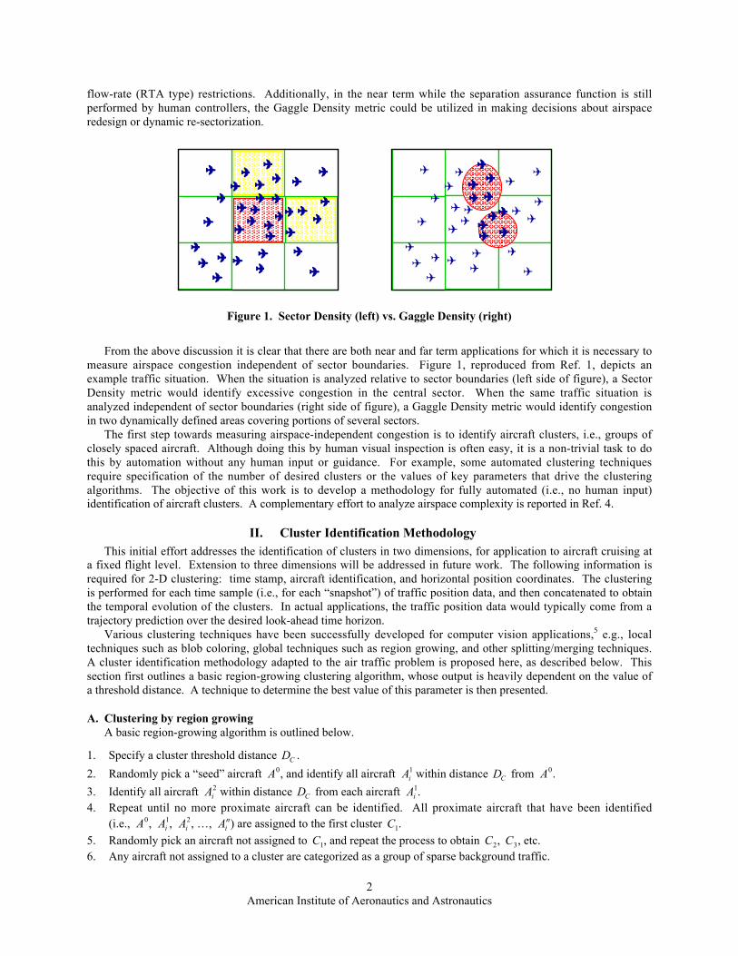
flow-rate (RTA type) restrictions. Additionally, in the near term while the separation assurance function is stillperformed by human controllers, the Gaggle Density metric could be utilized in making decisions about airspaceredesign or dynamic re-sectorization.

Figure 1. Sector Density (left) vs. Gaggle Density (right)

From the above discussion it is clear that there are both near and far term applications for which it is necessary tomeasure airspace congestion independent of sector boundaries. Figure 1, reproduced from Ref. 1, depicts anexample traffic situation. When the situation is analyzed relative to sector boundaries (left side of figure), a SectorDensity metric would identify excessive congestion in the central sector. When the same traffic situation isanalyzed independent of sector boundaries (right side of figure), a Gaggle Density metric would identify congestionin two dynamically defined areas covering portions of several sectors.

The first step towards measuring airspace-independent congestion is to identify aircraft clusters, i.e., groups ofclosely spaced aircraft. Although doing this by human visual inspection is often easy, it is a non-trivial task to dothis by automation without any human input or guidance. For example, some automated clustering techniquesrequire specification of the number of desired clusters or the values of key parameters that drive the clusteringalgorithms. The objective of this work is to develop a methodology for fully automated (i.e., no human input)identification of aircraft clusters. A complementary effort to analyze airspace complexity is reported in Ref. 4.

II. Cluster Identification MethodologyThis initial effort addresses the identification of clusters in two dimensions, for application to aircraft cruising at

a fixed flight level. Extension to three dimensions will be addressed in future work. The following information isrequired for 2-D clustering: time stamp, aircraft identification, and horizontal position coordinates. The clusteringis performed for each time sample (i.e., for each “snapshot”) of traffic position data, and then concatenated to obtainthe temporal evolution of the clusters. In actual applications, the traffic position data would typically come from atrajectory prediction over the desired look-ahead time horizon.

Various clustering techniques have been successfully developed for computer vision applications,5 e.g., localtechniques such as blob coloring, global techniques such as region growing, and other splitting/merging techniques.A cluster identification methodology adapted to the air traffic problem is proposed here, as described below. Thissection first outlines a basic region-growing clustering algorithm, whose output is heavily dependent on the value ofa threshold distance. A technique to determine the best value of this parameter is then presented.

A. Clustering by region growingA basic region-growing algorithm is outlined below.

1. Specify a cluster threshold distance

€

DC .

2. Randomly pick a “seed” aircraft

€

A0, and identify all aircraft

€

Ai1 within distance

€

DC from

€

A0.

3. Identify all aircraft

€

Ai2 within distance

€

DC from each aircraft

€

Ai1.

4. Repeat until no more proximate aircraft can be identified. All proximate aircraft that have been identified(i.e.,

€

A0,

€

Ai1,

€

Ai2, …,

€

Ain) are assigned to the first cluster

€

C1.

5. Randomly pick an aircraft not assigned to

€

C1, and repeat the process to obtain

€

C2,

€

C3, etc.6. Any aircraft not assigned to a cluster are categorized as a group of sparse background traffic.

✈

✈

✈

✈✈

✈

✈

✈

✈✈

✈✈

✈

✈ ✈

✈

✈

✈

✈✈

✈

✈

✈✈

✈✈

✈✈

✈

✈

✈

✈✈ ✈

✈

✈

✈✈

✈

✈

✈

✈✈

✈✈

✈

✈ ✈

✈

✈

✈

✈✈

✈

✈

✈✈

✈✈

✈✈

✈

✈

✈

✈✈

American Institute of Aeronautics and Astronautics3

Although this clustering technique is simple to implement, its results are heavily dependent on the value of thethreshold distance

€

DC . Specifying different values of

€

DC will result in very different clustering patterns (in terms of

number, size, and membership of clusters). Hence the challenge is to determine the “best” value of

€

DC in anobjective and automated way.

B. Evaluating cluster qualityQualitatively speaking, a “good” cluster is one that is cohesive and well separated from other clusters; it is alsoeasily distinguishable from the background elements that do not belong to any cluster. In more objective terms, acluster is distinct if the average distance between in-cluster neighbors is significantly less than the average distancebetween cluster edge members and their nearest out-of-cluster neighbors. The neighbors of an element can beidentified in several ways; this work utilizes Delaunay Triangulation6 which is often used in computationalgeometry to determine neighboring elements within a set of points.

A triangulation of a set S of co-planar non-collinear points is a partition of the convex hull of S into triangles.While there may be many possible triangulations for the set S, there is a (generally) unique triangulation, called theDelaunay triangulation, with the property that the interior of the circumcircle of any triangle in the triangulationcontains no points of S. It can be computed by minimizing the standard deviations of the angles of the triangles,using 60 degrees (the angle of an equilateral triangle) as the mean. In this sense, the Delaunay triangulation is themost equi-angular triangulation – it minimizes long/thin triangles. The Delaunay triangulation is the dual structureof the Voronoi diagram, which describes a polygonal structure that defines the “domain of proximity” for eachelement in a set of points. For the purposes of this work, the Delaunay triangulation provides a map connecting eachpoint to its “natural” neighbors.

Figure 2. Evaluation of Cluster Quality

Consider the evaluation of a cluster pattern (for a snapshot of traffic) computed for some value of the thresholddistance

€

DC . Let this pattern have m clusters identified within a set of N elements (aircraft). For each cluster

€

C j , a

Delaunay Triangulation is performed; this establishes a connectivity diagram of members in the cluster (i.e.,

American Institute of Aeronautics and Astronautics4

identifies the natural neighbors of each member) and also determines the convex hull (i.e., identifies the edgemembers) of the cluster. Let the average of all distances between natural neighbors in cluster

€

C j be represented by

€

d j . Next, a Delaunay Triangulation is performed for the entire set of N aircraft (that includes all clusters and

background traffic). For each edge member in cluster

€

C j , the distance to the nearest out-of-cluster natural neighbor

is computed, and then the average over all edge members is computed and designated as

€

l j . Then, a goodness

metric for each cluster

€

C j is computed as the ratio

€

rj = (l j / d j ) . Figure 2 illustrates the quantities

€

d j and

€

l j . A

large value of

€

rj indicates that the cluster

€

C j is well separated from other clusters and/or background traffic.

Conversely, a small value of

€

rj , especially a value less than unity, indicates that the cluster

€

C j is not distinguishable

from other traffic. Finally, the Clustering Quality Metric

€

R is computed as the weighted (by number of aircraft inthe cluster) average of

€

rj over all clusters. It indicates the goodness of the overall cluster pattern corresponding to

the threshold distance

€

DC ; again, larger values are better. The best threshold distance

€

DC* is determined by

repeating the above process over a range of

€

DC values, and picking the one that yields the maximum value of

€

R .

The best cluster pattern is the one obtained from region-growth clustering with threshold distance

€

DC* .

III. Results and DiscussionThe clustering methodology described in the preceding section was implemented in software, and exercised

using a traffic scenario created from recorded field data. It is noted that actual applications of Gaggle Density toregulate automated separation assurance would identify clusters for predicted trajectories over some look-timehorizon. An 18-hour (6 am to midnight, local time, on a weekday) recording of track data was obtained for theCleveland Air Route Traffic Control Center (ZOB). These data records, obtained from the FAA’s Enhanced TrafficManagement System (ETMS), were approximately 1 minute apart. It is noted that the data recording was madeprior to implementation of domestic reduced vertical separation minimum (DRVSM) in January 2005. The data setincludes information on time stamp, aircraft identification, latitude, longitude, and flight level (information onaircraft velocity vector is also available, but not needed for this clustering analysis). In a simple representation of afuture traffic scenario with three times the current traffic, data for three flight levels (cruising traffic at FL 310,FL 330, FL350, and climbing/descending traffic in between) were collapsed to a single altitude. The aircraft countsfor this “3X density” traffic scenario are presented in Fig. 3, which shows the expected variation over the day (leftgraph) and the distribution (right graph).

Figure 3. Aircraft count for “3X density” traffic scenario: time history (left) and histogram (right)

American Institute of Aeronautics and Astronautics5

Next, the clustering methodology described in Section II was exercised using this traffic scenario. Arequirement for cluster membership of at least 5 aircraft was enforced to eliminate very small clusters. Theclustering logic searched over a range of threshold distances

€

DC between 10 nmi and 100 nmi (increments of

5 nmi) to find the value

€

DC* that yielded the best clustering quality as measured by

€

R . The final cluster pattern is

the one corresponding to region-growth clustering associated with

€

DC* . A cluster pattern was determined for each

“snapshot” of traffic in the ETMS data set, at 1-minute intervals from roughly 6 am to midnight local time,corresponding to over 1,000 time samples.

Figure 4. Cluster count for “3X density” traffic scenario: time history (left) and histogram (right)

Figure 5. Relationship between cluster count and aircraft count

American Institute of Aeronautics and Astronautics6

The results are presented in Fig. 4 (left), which shows clusters as a function of local time. Fig. 4 (right) showsthe distribution of cluster counts; for example, it indicates that for 30% of the time samples (traffic snapshots) therewere 2 clusters (plus some background traffic). For the data set analyzed, there were no more than 8 clusters for anytime sample. Figure 5 shows the relationship between aircraft counts and cluster counts. It can be seen that thenumber of clusters roughly tracks the aircraft count over time, as expected. An interesting observation from Fig. 5(right) is that, for the data set analyzed, the cluster count is typically no more than 10% of the aircraft count for anygiven time sample.

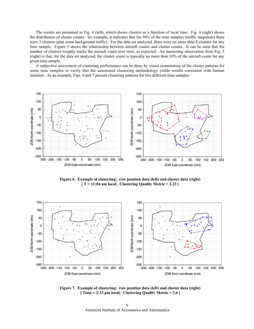
A subjective assessment of clustering performance can be done by visual examination of the cluster patterns forsome time samples to verify that the automated clustering methodology yields results consistent with humanintuition. As an example, Figs. 6 and 7 present clustering patterns for two different time samples.

Figure 6. Example of clustering: raw position data (left) and cluster data (right)[ T = 11:04 am local; Clustering Quality Metric = 2.23 ]

Figure 7. Example of clustering: raw position data (left) and cluster data (right)[ Time = 2:33 pm local; Clustering Quality Metric = 3.6 ]

American Institute of Aeronautics and Astronautics7

The quality of the clustering for a given time sample is represented by the Clustering Quality Metric,

€

R , whichindicates how well the clusters are separated from each other and background traffic. It is recalled that a large valueis good, while a value below unity is poor. Figure 8 shows the values of

€

R for each time sample. It can be seen thatall values are above unity, and the average value is approximately 2.3. This indicates good clustering performancebecause it implies that, on average, the distance between cluster edge members and their nearest out-of-clusterneighbors is more that twice the distance between in-cluster neighbors.

Figure 8. Clustering Quality Metric

Figure 9. In-cluster separation distances

American Institute of Aeronautics and Astronautics8

It is recalled that the identification of clusters is simply a first step towards identifying dynamic regions of highdensity/complexity airspace. Future work will address the determination of appropriate complexity metrics andcorresponding threshold levels of Gaggle Density to determine dynamic flow constraints for aircraft operating underautomated separation. However, a simple representation of cluster density distribution is given in Fig. 9, whichpresents the average separation distance between the members of each cluster. It is noted that the separationdistances on the ordinate of Fig. 9 are inversely related to cluster density – small distances correspond to denseclusters, while large distances correspond to sparse clusters.

Figure 10. Relationship between cluster quality and cluster density

Figure 10 is a cross-plot of the parameters presented in Figs. 8 and 9: it shows the relationship between clusterquality and cluster density. The ordinate of the left graph in Fig. 10 is the average separation distance between themembers of each cluster, while the reciprocal of this distance is shown on the ordinate of the right graph. It can beseen that high density (closely spaced) clusters are generally of high quality (i.e., well separated from other clustersand background traffic); this is consistent with intuition. This correlation is beneficial, because it is the high-density clusters that are of primary interest in Gaggle Density analysis.

IV. ConclusionA methodology for automated identification of aircraft clusters has been presented. This is the first step towards

the utilization of Gaggle Density as a sector-independent measure of airspace congestion. The cluster identificationmethodology utilizes a region-growth clustering method whose key parameter, a threshold distance, is determinedby maximizing a clustering quality metric. Example results were presented based on field data for ClevelandCenter. Preliminary results indicate that, for the data sample analyzed, the clustering methodology yields goodperformance.

AcknowledgmentsThe authors thank Steve Green of NASA Ames for valuable discussions on the concept of Gaggle Density, and

Michael Jastrzebski of UC–Santa Cruz for generating final results.

References1Green, S.M., Bilimoria, K.D., and Ballin, M.G., “Distributed Air/Ground Traffic Management for En Route Flight

Operations,” Air Traffic Control Quarterly, Vol. 9, No. 4, 2001, pp. 259–285.

American Institute of Aeronautics and Astronautics9

2Erzberger, H. and Paielli, R.A., "Concept for Next Generation Air Traffic Control System." Air Traffic Control Quarterly,Vol. 10, No. 4, 2002, pp. 355-378.

3Kopardekar, P. and Magyarits, S., “Measurement and Prediction of Dynamic Density,” 5th USA/Europe Air TrafficManagement R&D Seminar, Budapest, Hungary, June 2003.

4Ishutkina, M.A., Feron, E., and Bilimoria, K.D., “Describing Air Traffic Complexity Using Mathematical Programming,”Paper No. 2005-7453, AIAA Aviation Technology, Integration, and Operations Conference, September 2005.

5Ballard, D.H. and Brown, C.M., Computer Vision, Prentice-Hall, Englewood Cliffs, NJ, 1982, pp. 149–165.6Preparata, F.P. and Shamos, M.I., Computational Geometry: An Introduction, Springer-Verlag, New York, 1985.