American Institute of Aeronautics and Astronautics
1
A Model for Determining the Cost of National Airspace System Maintenance Service Levels
Myron Hecht
The Aerospace Corporation, El Segundo, CA 90245
Abstract: A model that predicts staffing requirements in the National Air Space (NAS) Facilities using three sub-models (preventative maintenance, watch-standing, and corrective maintenance) is described. The means by which service metrics can be defined using these models is proposed, and the benefit of being able to use these service metrics as a basis for predicting the cost of service is explained. The results of this model can be used to estimate the cost of meeting Service Level Agreements between the maintainers and users of NAS facilities and services.
Nomenclature ∆ = time interval µ = average repair rate (the reciprocal of the average repair time) λout = reciprocal of MTBOunsched {PM} = set of all preventative maintenance tasks. {t} = set of all time intervals in which the activity is less than the threshold ordered by increasing time. ath = threshold activity level below which facilities can be taken down for maintenance c' = a real number representing the average number of specialists across multiple shifts (real number) c = average staffing level for each sector maintenance center (SSC) (integer) DW = duration of the maintenance window defined in the previous section. DW,i,j , = duration of the maintenance window for the the jth period in the ith
discipline fk = frequency of the kth task fmax = frequency of the most frequently required critical maintenance task (typically once per day or 1) i = index representing the technical disciplines of specialists (automation, CNS, environmental) indexmax = index of t max indexmin = index of t min Li = number of specialists in the ith discipline assigned to the shift when the maintenance window occurs. MCM = number of specialists required to perform corrective maintenance within a given response time Mi = average number of specialists of the ith discipline on watch during the maintenance window MPM = number of personnel specialists for preventative maintenance (PM) tasks MTBOunsched = reported value for unscheduled outages for a specific facility or facility Mwatch-standing = number of specialists required for watch-standing N = total number of specialists required at the site n = number of facilities in each cost center Ni = number of periods over which the duration is averaged for the ith discipline Nrepair (t) = number of facilities having a repair time of t (actually, in the interval between t and t+dt) Ntot = total number of facilities that have failed and are being repaired. pm = element of {PM} characterized by a facility, duration, criticality, required frequency, discipline, special qualifications, priority, and impact. po = probability of empty queue (specialist being available) s2, s1 = roots of pr in the interval (0..24]* T = time over which the outage time is measured, tcycle = cycle time for the start of the shift cycle (typically 24 hours)
* The (..] notation is intended to convey that the interval is inclusive of 0:00 to 23:59 but exclusive of 24:00 which is actually 0:00 of the next day
AIAA 5th Aviation, Technology, Integration, and Operations Conference (ATIO) <br>26 - 28 September 2005, Arlington, Virginia
American Institute of Aeronautics and Astronautics
2
tk = duration of the k th task measured in hours. tk,crit = time required for the k th critical task in the ith discipline. tmax = max({t}) such that there is at least one adjacent preceding value, i.e., t max-tmax-1 = ∆. tmax,crit = maximum duration of the tasks in {PM} tmin = min({t}) such that there is at least one adjacent subsequent value, i.e., tmin+1-tmin = ∆. ts = time of day (GMT) ttravel1way = average 1-way travel time for the region tunsched = unscheduled outage time Uo = steady state utilization for a finite queue v3..v8 = the regression constants emerging from a least squares fitting function w = specialist overhead. x = ratio of unscheduled outages to total outages for the SSC (or other unit under consideration) z = number of specialis ts required to populate a continuous position λ = model failure rate µ = model repair time
I. Introduction HIS paper describes a model in which the quality of maintenance and sustainment service is related to the resources required for providing the service. Maintenance on National Airspace System (NAS) facilities
consumes a significant portion of the FAA’s annual operations budget. While the number of FAA facilities continues to grow, continuing budget pressure constrains the growth in maintenance resources – particularly in staffing. Thus, there is a need to develop a systematic approach to using maintenance resources efficiently. This paper describes a conceptual approach and an analytical model for performing such analyses. The following section provides an overview of the model. Sections III through V describe the constituent sub-models, and Section VI describes in general terms how service metrics can be derived from these models and how the resultant costs for providing a service level defined by these metrics can be predicted. The final section provides concluding remarks and describes plans for future work.
II. Model Overview The field maintenance force consists of Federal Aviation Administration (FAA) emp loyees organized as a
hierarchy consisting of 9 regions. Each region consists of a number of System Maintenance Offices (SMOs) which manage lower level System Service Centers (SSCs). Facilities (a “facility” is the term the FAA uses for equipment, infrastructure or structures used for air traffic surveillance, navigation, communication, or control) are allocated to accounting cost centers within the SSC. This set of facilities might be located at one large airport or might be geographically dispersed among a number of small airports. When technicians, referred to in the FAA as “specialists”, are not co-located with equipment, then travel time must be considered as part of the maintenance work load. Because NAS facilities are varied and complex, not all specialists are qualified to fix repair all equipment allocated to their SSC or SSU. Instead, specialists limit their scope of expertise to specialty categories defined as communications, navigation (including landing systems), surveillance, automation (i.e., computer technology) or infrastructure (such as lighting, engine generators, power and environmental systems, etc).
Specialists engage in three broad types of activities: watch-standing (i.e., a specialist actually being present at an FAA facility and at the ready to perform maintenance at any time), preventative maintenance (PM), and corrective maintenance (CM). Both watch-standing and PM activities are scheduled; CM actions are undertaken in response to failures during operation and may be either scheduled or unscheduled. The model discussed here predicts the staffing requirement for each discipline in terms of three components: watch-standing, preventative maintenance and unscheduled CM (scheduled CM tasks are treated as PM tasks). That is ,
∑ ++=i
iCMidingwatchsiPM MMMN ,,tan, Equation 1
where N is the total number of specialists required, i is the index representing the technical disciplines of specialists (automation, CNS, environmental), MPM is the number of personnel specialists for PM tasks, Mwatchstading is the
T
American Institute of Aeronautics and Astronautics
3
number of specialists required for watch-standing, and MCM is the number of specialists required to perform unscheduled CM tasks within a given response time.
Under many maintenance philosophies, when specialists are standing watch, they can perform PM. If so, then Equation 1 becomes
∑ +=i
iCMidingwatchsiPM MMMN ,,tan, ),max( Equation 2
The sub-models for the MPM,,j , Mwatch-standing and MCM terms are described in Sections III, IV, and V respectively.
III. PM Sub-Model The PM sub-model determines how many specialists in each specialty category will be needed to perform the scheduled maintenance requirements of the SSC. The first subsection describes the concept of a maintenance window, the low activity period during which scheduled maintenance tasks can be performed. The second describes the method for defining the length of the maintenance window, and the third describes an algorithm for determining whether it is feasible to schedule all maintenance tasks within the window. The fourth contains concluding remarks on non-labor PM costs, accounting for travel time, and alternative scheduled maintenance metrics.
A. Maintenance Window
Some PM activities, referred to as critical tasks, are restricted as to their scheduling. The usual reason is that such tasks require taking a facility off-line or have a substantial likelihood of causing the equipment to go down. At all major NAS facilities, there is some period of daily low activity surrounded by periods of higher activity. Maintenance is performed at periods of minimum activity. The maintenance window is determined by the interval between the earliest and the latest times at which activity at the facility is below an activity threshold as shown in Figure 1. The ordinate (y-axis) shows traffic activity measured as flights per hour, and the abscissa (horizontal axis) shows the time of day (as Greenwich Mean Time, or GMT). As the activity threshold is raised, the maintenance window size is increased. Thus, as shown in the figure, as the activity threshold is increase from 10 (Window 1) to 20 aircraft per hour (Window 2), the maintenance threshold increases from 6 to 8 hours.
0
5
10
15
20
25
30
35
12:00:00AM
2:00:00AM
4:00:00AM
6:00:00AM
8:00:00AM
10:00:00AM
12:00:00PM
2:00:00PM
4:00:00PM
6:00:00PM
8:00:00PM
10:00:00PM
Time of DAY (GMT)
Act
ivit
y
Activity Data 6th degree polynomial fit 5th degree polynomial fit
Figure 1. Maintenance Window and Activity Threshold
Window 2
Window 1
Act
ivit
y th
resh
old
American Institute of Aeronautics and Astronautics
4
B. Calculating the Size of maintenance Window as a Function of the Activity Threshold
The size of the maintenance window can be determined analytically by using a least squares polynomial fit to model the traffic activity and then setting it equal to an threshold below which maintenance is allowed and above which maintenance is forbidden, i.e.,.
342
53
64
75
8 vtvtvtvtvtva ssssth +++++= -
Equation 3
where ath is the traffic threshold below which maintenance activity is allowed, v3..v8 are the regression constants emerging from a least squares fit ting function of the traffic activity (see Figure 1), and ts is the time of day (GMT).
This equation can be rearranged , i.e.,
0342
53
64
75
8 =−+++++ thssss avtvtvtvtvtv -
Equation 4
and solved to find the roots of the polynomial. In most cases, there will be only two real valued roots within the interval of interest (0..23:59).
The maintenance interval can then be found by
Dw = s2 – s1 Equation 5
where Dw is the maintenance window resulting from the value of ath, s2 and s1 are the real roots of Equation 4, and s2 > s1.
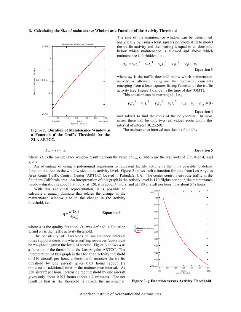
An advantage of using a polynomial regression to represent facility activity is that it is possible to define function that relates the window size to the activity level. Figure 2 shows such a function for data from Los Angeles Area Route Traffic Control Center (ARTCC) located in Palmdale, CA. The center controls en-route traffic in the Southern California area. An interpretation of this graph is the activity level is 110 flights per hour, the maintenance window duration is about 3.8 hours, at 120, it is about 4 hours, and at 180 aircraft per hour, it is about 5 ½ hours.
With this analytical representation, it is possible to calculate a quality function that relates the change in the maintenance window size to the change in the activity threshold, i.e.,
)()D(
qth
w
add
= Equation 6
where q is the quality function, Dw was defined in Equation 5, and ath is the traffic activity threshold.
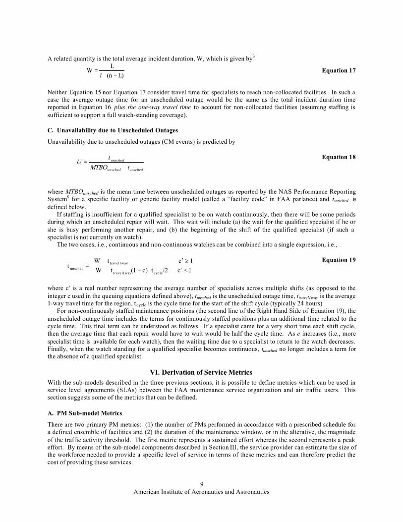
The sensitivity of thresholds to maintenance interval times supports decisions where staffing resources (cost) must be weighted against the level of service. Figure 3 shows q as a function of the threshold at the Los Angeles ARTCC. The interpretation of this graph is that for at an activity threshold of 110 aircraft per hour, a decision to increase the traffic threshold by one aircraft gives 0.03 hours (about 1.8 minutes) of additional time in the maintenance interval. At 220 aircraft per hour, increasing the threshold by one aircraft gives only about 0.021 hours (about 1.2 minutes). The net result is that as the threshold is raised, the incremental
120 140 160 180 200 2203.5
4
4.5
5
5.5
6
6.5Maintenance Window vs. Threshold
Activity Threshold
Dur
atio
n of
Mai
nten
ance
Win
dow
6 .411
3.799
Intrvl thshld( )
2 threshold⋅threshold thshld
Figure 2. Duration of Maintenance Window as a Function of the Traffic Threshold for the ZLA ARTCC.
100 120 140 160 180 200 2200.02
0.021
0.022
0.023
0.024
0.025
0.026
0.027
0.028
0.029
0.03
0.031
Activity Threshold
q fu
nctio
n
0.03
0.02
thrshldIntrvl thrshld( )
d
d
220110 thrshld
Figure 3. q Function versus Activity Threshold
American Institute of Aeronautics and Astronautics
5
benefit of increasing the duration of the maintenance window is reduced.
C. Feasibility of Performing PM Tasks in the Maintenance Window
The next step is to determine the staffing required for the selected maintenance window size. The analysis is done at the level of an SSC and is based on the following assumptions:
1. The SSC is responsible for preventative maintenance on all facilities in the FSEP that are assigned to the cost centers associated with it
2. The required preventative maintenance tasks† for each facility within the SSC are characterized in terms of Location ID (to account for location-specific values) facility code, duration, criticality‡, required frequency, and priority§
3. The specialists including specialty and qualifications within each SSC are known and contained within a technical file.
The maintenance schedule will be feasible if the following conditions are met: 1. Critical task duration feasibility: The duration of the longest critical maintenance task is less than the
duration of the maintenance window.
2. Workload feasibility: The sum of the duration of (a) critical PM tasks is less than or equal to the available specialist hours in maintenance windows and (b) all PM tasks is less than or equal to the total available specialist hours
3. Schedule feasibility: With the posited maintenance staff, it is possible to arrange (a) a schedule of critical PM tasks they can all be performed during maintenance windows with the required frequency and (b) all tasks such that they can be performed with the required frequency.
Clearly, if the third (schedule feasibility) condition is satisfied, then the first two conditions are also satisfied. However, finding the required staff size is an iterative process and therefore, determining whether the first two conditions are true is simpler than determining schedule feasibility. Hence, for computational simplicity, the assessment process is to first evaluate of task duration and workload feasibility (conditions 1 and 2) and only if conditions are met, to evaluate schedule feasibility. The details for testing each of these conditions are discussed in the following subsections. 1. Task duration feasibility
The test for task duration feasibility can be stated verbally as “can the longest duration critical task (i.e., task that must be performed during the low activity period) be performed within the contemplated maintenance window”? and mathematically as
tmax, crit ≤ DW Equation 7 where {PM} is the set of relevant preventative maintenance tasks each element of which is characterized by a facility, duration, criticality, required frequency, discipline, special qualifications, priority, and impact, tmax, crit is the maximum duration task within {PM}, and DW is the duration of the maintenance window defined in the previous section. When critical PM tasks are performed at a remote location, the round-trip travel time must also be included for each location visited. 2. Workload Feasibility
The workload feasibility condition is met if (1) the total task workload can be met by the amount of staffing in the SSC and (2) the critical task workload can be done within the maintenance interval.
† For the purposes of this discussion, a “task” is considered to be all the activities related to a PM performed by one specialist at the same time on a single facility. The duration of the task is the time needed to perform all of these activities.
‡ The criticality affects whether it is permissible for the task to be performed outside of the maintenance window (critical tasks must be performed within the window). § The priority level determines whether the task can be pre-empted by another task.
American Institute of Aeronautics and Astronautics
6
For the total task workload, the feasibility condition is that there must be sufficient specialist time to perform all PM tasks. In addition, only qualified specialists can perform the PM tasks in each specialty area. This can be stated mathematically as
∑=
≥+⋅
⋅L
kk
ki tff
wzM
1 max)1(24 Equation 8
where 24 is the number of hours in a day (assuming that the tk term on the right hand side is given in hours), Mi is the average number of specialists of the ith discipline on watch during the maintenance window, z is the number of specialists required to populate a continuous position (i.e., 24 hours per day, 7 days per week), currently equal to 7 specialists, fk is the frequency of the k th task (where the frequency is the inverse of the required interval; for a biweekly task, fk would be 1/14), fmax is the frequency of the most frequently required critical maintenance task (typically once per day or 1), tk is the duration of the kth task measured in hours, and w is the specialist overhead. The quantity of 1/(1+w) is a “de-rating factor” or margin that accounts for two components: (1) a desired margin to ensure that specialists are not dedicated to only performing PM tasks during the watch but also have sufficient time to respond to unscheduled outages, and (2) additional unanticipated condition factor which accounts for the fact that conditions such as weather, illness, security emergencies, or other unanticipated events may in fact reduce the effect available workforce. In short, interpretation of equation 8 is that the number of “effective specialist hours” per 24 hour period (left-hand side) must be at least as large the average daily scheduled PM work load measured in hours (right-hand side).
For critical tasks (that must be performed in the maintenance window), the PM workload is a subset of all tasks. Also, the available time, i.e., the maintenance window is a subset of the entire day. Just as was the case with all maintenance tasks, critical task maintenance intervals vary, and because not all critical PM tasks are done with the same frequency, the maintenance intervals and total workload are averaged. Taking into account these considerations, the feasibility condition becomes
∑∑==
≥⋅+
L
kcritk
kjiW
N
ji
i tffD
NwL i
1,
max,,
1
1)1(
Equation 9
where Li is the number of specialists in the ith discipline actually assigned to the shift in which the maintenance window occurs (note that this is slightly different than the Mi/c used in Equation 8), Ni is the number of periods over which the duration is averaged (typically 365 daily periods) for the ith discipline, DW,i,j , is the duration of the maintenance window for the the jth period in the ith
discipline, tk,crit is the time required for the k th critical task in the ith discipline. Note that the tasks for all equipment in the SSC should be included in the summation, and w, fk and fmax are as defined above.
The interpretation of Equation 9 is similar to Equation 8, i.e., that the “effective specialist hours” must be greater than or equal to the average critical PM workload. However, here, replacing the value “24” is the average maintenance window duration, and replacing the quantity Mi/c(1+w) , the average specialist presence, is the average number of specialists actually present on the watch in which maintenance window occurs. The right hand side is the sum of all tasks that need to be performed in the maintenance window (i.e., critical tasks) normalized for the frequency by which they need to be performed.
3. Schedule Feasibility
Once task duration and workload feasibility have been established, the final condition can be checked, i.e., that it is possible to create a maintenance schedule that will enable all tasks to be performed at a given level of staffing. The approach in the model is to create schedule that is not necessarily optimal, but demonstrates the feasibility of performing all required tasks with the given staffing. Figure 4 is a graphical depiction of the algorithm, which is based on the concept of finite capacity daily “bins.” The bins represent the amount of PM labor for that discipline available on that that day (for all tasks) or the number of specialist hours available during the maintenance window (for critical tasks). A task that is scheduled is been placed in an appropriate bin, and the available capacity of that bin is reduced. The process is repeated for successive lower frequency tasks are placed in the bins.
For all tasks, a bin is available on each day that an SSC is staffed, and its duration is the number of specialist hours available on that day. The most frequently executed tasks (i.e., daily tasks) are placed in the bins, then
American Institute of Aeronautics and Astronautics
7
successively lower frequencies of tasks are placed in the appropriate bins until the capacity of the bin is exceeded (i.e., whether there are insufficient maintenance hours available on the specified date to perform the task). If not, a search is made for the next available “bin
If there is no capacity in the bin for that task, a search is made for an adjacent bin. The search alternates for bins to the right and left (numerically, bin index lower, then two higher, then three lower, etc.) until either (a) a bin is found, or (b) a frequency factor limit is reached.
Schedule feasibility is first performed for the entire task set and then again for the critical tasks. A schedule is feasible once all tasks have been placed in bins and no bin capacity is exceeded. A schedule is infeasible if one or more tasks can not be placed in bins after the available bin search is performed.
Task beingscheduled
Tasks not yetscheduled
Scheduledtasks
Next step of freebin space search
(if necessary)free bin spacesearch
Figure 4. Graphical Depiction of Rough Scheduling Algorithm
IV. Watch-Standing Sub-Model The watch-standing sub-model calculates the required staffing for the facilities in the SSC or SSU. Watch-standing requirements for each facility are set by the FAA and documented as restoration codes in the Facility, Services and Equipment (FSEP) database.1 Both the type of facility and the traffic level handled by the facility are factors in determination of the restoration code. A facility such as an approach control center handling traffic at a busy metropolitan airport may require continuous (24 hours per day, 7 days per week) coverage, but a lightly used navigation aid in a rural area may require watch-standing only during normal business hours.
Within an SSC, there is adequate coverage on-site maintenance requirements if, for each discipline required by the facility at the SSC, there is coverage for the facility requiring the maximum coverage, that is,
Mi,on-site ≥ z⋅max (df⋅hf/168) Equation 10
where Mi is the number of specialists (specialists) assigned to that SSC, z is the number of specialists required to provide a single specialist presence continuously (usually 7 specialists per each continuously present individual), max (d f) is the number of days per week of on-site specialist presence associated with maximum restoration code (usually 5 or 7) for on-site specialists SSC, max (hf) is the number of hours per day of on-site specialist presence associated with the maximum restoration code (8, 16, or 24), and 168 is the number of hours per week.
Equation 11 describes the staffing requirement for on-call (off-site but available) maintenance resources
Mi,on-call ≥ z⋅max (df⋅hf/168) Equation 11 where the nomenclature is the same as that used in Equation 10.
We have made an assumption earlier that specialists who are on-call can also be performing PM actions during the maintenance window. If specialists performing watch-standing can not perform routine maintenance, then the coverage requirement would simply be
Mi,on-site,critical≥1 Equation 12
for all disciplines and for all required locations in the SSC. If more than one specialist must be on call, then the right- hand side of Equation 12 can be replaced with the required minimum on-call number.
American Institute of Aeronautics and Astronautics
8
V. Unscheduled CM Sub-Model The unscheduled maintenance sub-model predicts the following quantities for unscheduled repairs:
1. Average number of outstanding repairs (Unscheduled CM actions) 2. Average numb er of incidents awaiting repair (i.e., Unscheduled CM actions excluding those currently being
worked) 3. Unavailability due to unscheduled outages
Unlike the two sub-models that were based primarily on deterministic data (i.e., projected staffing schedules,
facility inventories, etc.), these metrics are based on random events and therefore rely on a predictive models. Two alternative approaches are possible: analytical approach based on queuing theory5 7 or a discrete event simultation. The analytical queuing model has the advantage of much shorter computation times and consistent results. The disadvantage of the queuing model is that it can not easily handle non-heterogeneous failure rates, pre-emption, and non-uniform staffing, although use of average quantities can overcome these problems (with some loss of accuracy). At present, the level of accuracy of maintenance data does not warrant a more detailed discrete event simulation approach although as maintenance data quality improves, such an approach can be used.2
The following subsections discuss the three metrics listed above using the analytical queuing approach.
A. Average Number of Outstanding Unscheduled CM Actions
The expected number of unscheduled CM actions that are both being fixed and awaiting response by a specialist is the equivalent of the queue length and is given by
⋅
−⋅⋅+
⋅
−⋅−⋅= −
−
=
−
=∑∑
i
ci
1c
0i
i1c
0io µc
1i)!(ni!
n!i
c!1
µi)!(ni!n!
i)(cpLλλ Equation 13
where L is the expected number of outstanding unscheduled CM actions, and po is the probability of a specialist being available for repair (the probability of an empty queue)and is given by 3
po
= 0
c-
i=
.!n!!i! !( )n - i)!
λµ
i
i=c
n.1!n!
!( )n - i)!
1
.c( i- c) c!c!
λ
µ
i1
Equation 14
In both above equations, c is the number of specialists in the SSC; n is the number of facilities for which the SSC is responsible; λ is the average failure rate (i.e., the rate of occurrence of unscheduled outages) of all the facilities in the SSC, and µ is the average repair rate of the facilities in the SSC. Methods for calculating the failure rate using FAA databases such as NASPAS4 including corrections to account for the impacts of redundancy and scheduled maintenance was described in earlier work.5 6 When specialists are not collocated with the facilities under repair, µ , which represents the time that a specialist is occupied, includes both the repair time and the round-trip travel time.7
B. Average Response Time
The time waiting for the start of repairs is given by
L)(n
LW q
q −⋅=
λ Equation 15
where Lq is the number of unscheduled CM actions that are waiting and have not yet been responded to and is given by3.
⋅
−⋅−⋅+−= ∑
−
=
i1c
0ioq 1)!(ni!
n!i)(cpcLL
µλ Equation 16
American Institute of Aeronautics and Astronautics
9
A related quantity is the total average incident duration, W, which is given by3
L)(nL
W−⋅
=λ
Equation 17
Neither Equation 15 nor Equation 17 consider travel time for specialists to reach non-collocated facilities. In such a case the average outage time for an unscheduled outage would be the same as the total incident duration time reported in Equation 16 plus the one-way travel time to account for non-collocated facilities (assuming staffing is sufficient to support a full watch-standing coverage).
C. Unavailability due to Unscheduled Outages
Unavailability due to unscheduled outages (CM events) is predicted by
unschedunsched
unsched
tMTBOt
U+
= Equation 18
where MTBOunsched is the mean time between unscheduled outages as reported by the NAS Performance Reporting System8 for a specific facility or generic facility model (called a “facility code” in FAA parlance) and tunsched is defined below.
If staffing is insufficient for a qualified specialist to be on watch continuously, then there will be some periods during which an unscheduled repair will wait. This wait will include (a) the wait for the qualified specialist if he or she is busy performing another repair, and (b) the beginning of the shift of the qualified specialist (if such a specialist is not currently on watch).
The two cases, i.e., continuous and non-continuous watches can be combined into a single expression, i.e.,
<′⋅−+≥′+
=1c/2tc)(1tW1c tW
tcycletravel1way
travel1wayunsched
Equation 19
where c' is a real number representing the average number of specialists across multiple shifts (as opposed to the integer c used in the queuing equations defined above), tunsched is the unscheduled outage time, ttravel1way is the average 1-way travel time for the region, tcycle is the cycle time for the start of the shift cycle (typically 24 hours)
For non-continuously staffed maintenance positions (the second line of the Right Hand Side of Equation 19), the unscheduled outage time includes the terms for continuously staffed positions plus an additional time related to the cycle time. This final term can be understood as follows. If a specialist came for a very short time each shift cycle, then the average time that each repair would have to wait would be half the cycle time. As c increases (i.e., more specialist time is available for each watch), then the waiting time due to a specialist to return to the watch decreases. Finally, when the watch standing for a qualified specialist becomes continuous, tunsched no longer includes a term for the absence of a qualified specialist.
VI. Derivation of Service Metrics With the sub-models described in the three previous sections, it is possible to define metrics which can be used in service level agreements (SLAs) between the FAA maintenance service organization and air traffic users. This section suggests some of the metrics that can be defined.
A. PM Sub-model Metrics
There are two primary PM metrics: (1) the number of PMs performed in accordance with a prescribed schedule for a defined ensemble of facilities and (2) the duration of the maintenance window, or in the alterative, the magnitude of the traffic activity threshold. The first metric represents a sustained effort whereas the second represents a peak effort. By means of the sub-model components described in Section III, the service provider can estimate the size of the workforce needed to provide a specific level of service in terms of these metrics and can therefore predict the cost of providing these services.
American Institute of Aeronautics and Astronautics
10
B. Watch-standing Sub-model Metric
The primary watch-standing metric is the extent of watch-standing coverage that will be provided. The primary benefit of the watch-standing metric is minimizing down-time of significant facilities in the NAS due to unscheduled CM actions. As shown in Section IV, it is quite feasible to derive a staffing requirement from a watch-standing coverage metric as well as vice-versa. Thus, it is possible for the maintenance service provider and facility users to engage in an interchange in which the maintenance provider can state the cost of providing coverage and users can assess whether the cost is commensurate with the decreased downtime benefit.
C. Unscheduled CM Sub-model Metrics
The primary unscheduled CM metric is specialist response time. This quantity determines the duration of outages in excess of the actual repair time. Other quantities that would also be of significance to users are the average unscheduled CM backlog (i.e., how many repairs are outstanding) and unavailability due to CM. With the models described in Section V, it is possible to predict these quantities as a function of staffing levels and hence, the basis for predicting cost exists.
VII. Conclusions This paper has described a model which predicts the staffing required for a level of service as defined through a set of metrics for PM, watch-standing, and unscheduled CM. Staffing in turn can be related to cost, and is by far the largest component of maintenance cost. However, a complete set of models which is currently under development will include other components of maintenance cost (replacement parts and consumables) that will be added to complete the overall cost-of-service calculation. Feasibility of using these models with existing FAA databases has already been established, and currently, work is underway to both generate the necessary parameters for all of the SSCs and SSUs in the NAS and to incorporate them into software that implements this model.
References 1 FAA Order 6000.5C “Facility, Service and Equipment Profile”, January, 1993 2 M. Hecht and J. Handal, “A Discrete-Event Simulator for Predicting Outage Time and Costs as a Function of Maintenance Resources”, Proceedings of the 2002 Annual Reliability and Maintainability Symposium, Seattle, WA January, 2002 3 D.R. Gross and C.M. Harris, Fundamentals of Queuing Theory, 2nd Edition, Wiley, New York, NY, 1985 4 Volpe National Transportation Systems Center, NASPAS User’s Manual, Report No. WP-59-FA-326-1, 1997 5 M. Hecht and J. Handal, “Impact of Maintenance Staffing on Availability of the U.S. Air Traffic Control System”, Proceedings of the 2001 Annual Reliability and Maintainability Symposium, Philadelphia, PA Jan, 2001 6 D. Kececioglu, Reliability and Life Testing Handbook , Vol. 1 & 2, PTR Prentice Hall, Englewood Cliffs, NJ, 1993 7 M. Hecht, J. Handal, and F. Demarco, “An Analytical Model for Predicting the Impact of Maintenance Resource Allocation on National Airspace System Availability”, Transportation Research Board Conference Record , January, 2000 8 FAA Order 6040.15C, National Aerospace Performance Reporting System, Changes 1&2, Sept. 1995