45
| Date post: | 19-Dec-2018 |
| Category: |
Documents |
| Upload: | hoangxuyen |
| View: | 219 times |
| Download: | 0 times |

American option pricing with LSMalgorithm and analytic bias correction
Thesis paper
Written by: Balazs Kovacs
Applied mathematics
External Supervisor: Gabor Molnar-Saska
Starts and Modeling, Morgan Stanley
Internal Supervisor: Herczegh Attila
Department of Probability Theory and Statistics
Eotvos Lorand University, Faculty of Science
Eötvös Loránd University
2012

I am grateful to Gabor Molnar-Saska for his endless support and inspiration and
thankful to Attila Herczegh for his useful remarks.
2

Contents
1 Introduction 4
2 Valuing options 6
2.1 European options . . . . . . . . . . . . . . . . . . . . . . . . . . . . . . . . 6
2.2 Valuing European options . . . . . . . . . . . . . . . . . . . . . . . . . . . 7
2.3 American options . . . . . . . . . . . . . . . . . . . . . . . . . . . . . . . . 8
3 Analysis of LSM algorithm 11
3.1 Modeling framework . . . . . . . . . . . . . . . . . . . . . . . . . . . . . . 11
3.2 Snell-envelope . . . . . . . . . . . . . . . . . . . . . . . . . . . . . . . . . . 12
3.3 LSM algorithm . . . . . . . . . . . . . . . . . . . . . . . . . . . . . . . . . 13
3.4 Convergence results . . . . . . . . . . . . . . . . . . . . . . . . . . . . . . 15
3.5 Least squares regression . . . . . . . . . . . . . . . . . . . . . . . . . . . . 16
3.6 The bias of LSM . . . . . . . . . . . . . . . . . . . . . . . . . . . . . . . . 21
4 Analytic bias correction 25
4.1 How biased is it? . . . . . . . . . . . . . . . . . . . . . . . . . . . . . . . . 25
4.2 Process of analytic bias correction . . . . . . . . . . . . . . . . . . . . . . 27
4.3 The bias term . . . . . . . . . . . . . . . . . . . . . . . . . . . . . . . . . . 29
4.4 Implementation of the new approach . . . . . . . . . . . . . . . . . . . . . 31
4.5 Testing of the new approach . . . . . . . . . . . . . . . . . . . . . . . . . . 34
4.6 Areas of further research . . . . . . . . . . . . . . . . . . . . . . . . . . . . 35
5 Conclusion 37
A Implementations 38
B Figures 42
Bibliography 45
3

Chapter 1
Introduction
Modern nancial markets oer a wide range of derivative products besides traditional
assets such as bonds and equities. These instruments are traded in over-the-counter mar-
kets by investment banks to hedge funds, commercial banks and government entities.
Investment banks hire mathematicians called strategists who are responsible for the pric-
ing and risk management of these products mainly using tools from statistics, probability
theory and stochastic calculus. This rapidly growing new branch of mathematics is often
referred to as quantitative nance.
The pricing of American style contingent claims has been one of the most popular
research topics for the last decades. The objective, particularly for an American option,
is to determine the optimal exercise strategy that maximizes the payo. This in fact
is a challenging task given the stochastic nature of the underlying. As a result of the
extreme development of information technology, simulation methods are gaining grounds
in derivative pricing as well. LSM algorithm introduced by Longsta and Schwartz is
the most well known and widely used Monte Carlo method for calculating American
option prices. LSM deals with the problem of re-simulation and provides a exible and
computationally tractable model for pricing. However, it does not consider the embedded
foresight bias, which is a product of the backward nature of the calculation along with
the Monte Carlo error of simulation.
My goal is to introduce a model based on LSM algorithm, that possesses all the good
qualities of the original method and also addresses the problem of the look ahead bias.
In the second chapter, I will review the basic nancial denitions and the well known
result of Black and Scholes on European option pricing, followed by a brief summary of
modeling and pricing diculties of American options. The third chapter begins with the
presentation of the modeling framework and LSM algorithm. After a profound analysis of
the least squares regression method I will attempt to study the impact of the look ahead,
which causes the algorithm to be super-optimal. In the fourth chapter, motivated by
Fries's concept, I develop a new six-step analytic approach to approximate the conditional
4

expectation of continuation which also eliminates the foresight bias. Subsequently, I will
present sucient testing that justies the accuracy of the new method, after which I
conclude with areas of further research.
5

Chapter 2
Valuing options
I am going to start with a brief introduction to the most important denitions and
concepts which are crucial to understand in the topic of derivative pricing. Quantita-
tive nance is a relatively new branch of mathematics that is fundamentally based on
probability theory, statistics and nance and it is mainly applied in the eld of modeling
stochastic processes and uncertainty in a nancial market environment. This chapter
summarizes the essential basics which are used in later chapters and strongly relies on
the work of Hull [2011].
A nancial derivative instrument denes a contract between two parties for future
transactions of securities, assets or payments. Particularly an option species a deal
on an asset at a reference price. The buyer of the option purchases the right, but not
the obligation, to engage in the transaction, but once the option is exercised the seller
of the contingent claim is obligated to fulll the transaction. Based on the common
characteristics of dierent type of payo functions of the options, they are referred to
as European, American, binary or barrier; just to name a few of the prevalent naming
conventions.
2.1 European options
A European option provides the right but not the obligation, to buy or sell one unit
of the underlying at a predetermined date at a reference price. This one exercise date
is referred to as maturity, the underlying is generally a stock and the reference price is
called the strike. Whether the option conveys the right to sell or to buy, it is refereed to
as:
European call option: provides the opportunity to buy one unit of the underlying at
maturity, thus it's payo function is (S(T )−K)+ and it's value at time t is denoted
by C(S, t, T,K)
6

European put option: provides the opportunity to sell one unit of the underlying at
maturity, thus it's payo function is (K−S(T ))+ and it's value at time t is denoted
by P (S, t, T,K)
where S(t) is the underlying asset's spot price at t, T is the time of maturity and K is
the strike. Call and put options with the same maturity and strike are in close relation
on liquid markets, this is represented by the put-call parity equation:
P (S, t, T,K) = C(S, t, T,K) +K ·B(t, T )− S(t) (2.1.1)
where B(t, T ) is the value of the bond at time t that matures at T . Furthermore, if the
bond interest rate r, is assumed to be constant, then the above relationship simplies to:
P (S, t, T,K) = C(S, t, T,K) +K · e−r(T−t) − S(t)
2.2 Valuing European options
Assume that the stock price dynamics is summarized by the following stochastic dif-
ferential equation:
dS(t) = µ · S(t)dt+ σ · S(t)dW (t) (2.2.1)
which is equivalent to the stock price following a geometric Brownian motion:
S(t) = S(0) · exp[(µ− σ2
2)t+ σW (t)
](2.2.2)
where µ is the long term return, the drift term of the stock price and σ is the volatility
of the underlying. Uncertainty is modeled by the increments of the standard Brownian
motion.
A trading strategy in nance is a set of rules determining when to buy or sell in-
struments on the market. For instance, a delta neutral strategy aims to reduce the risk
associated with the price movements of the underlying stock by maintaining 0 delta for
the total portfolio. Delta is the measure of how the price of the derivative, particularly
the option price changes as a result of a change in the price of the underlying. Mathe-
matically speaking it equals to the partial derivative of the option's value with respect
to the price of the underlying stock. Thus, such portfolio typically consists of an option
and the underlying stock such that the positive and negative deltas oset; consequently,
the portfolio value is unchanged by small price changes of the underlying. Since the delta
hedge portfolio is risk-less, Black and Scholes [1973] argued that the rate of return of this
strategy has to equal to the risk free rate otherwise this would provide an opportunity
7

for a risk free prot or equivalently arbitrage. With the aid of Ito [1951] lemma this lead
them to the well know partial dierential equation published in 1973 referred to as the
Black-Scholes equation:
∂V
∂t+
1
2σ2S2 ∂
2V
∂S2+ rS
∂V
∂S− rV = 0 (2.2.3)
where V , the value of the derivative, has two arguments: time t and spot price of the
underlying S(t). Equation (2.2.3) holds true for any European style derivative whose
payo only depends on the value of the underlying at maturity, where S(t) follows (2.2.2),
i.e. it is a geometric Brownian motion, with constant drift and volatility. The value of a
European option on a non-dividend paying stock is obtained by solving the above partial
dierential equation with the appropriate boundary conditions, specically V (T, S) =
C(S, T, T,K) = (S(T ) − K)+ for a call or (K − S(T ))+ for a put. Hence, the Black-
Scholes formula for a European call option value is:
C(S, t, T,K) = Φ(d1)S(t)− Φ(d2)Ke−r(T−t) (2.2.4)
where Φ(·) is the cumulative distributive function of the standard normal distribution
and d1 and d2 are:
d1 =ln(S(t)K ) + (r + σ2
2 )(T − t)σ√T − t
d2 =ln(S(t)K ) + (r − σ2
2 )(T − t)σ√T − t = d1 − σ
√T − t
Then, I just simply use the put-call parity to derive the value of a European put option:
P (S, t, T,K) = C(S, t, T,K) +K · e−r(T−t) − S(t) =
Φ(−d2)Ke−r(T−t) − Φ(−d1)S(t)
Consequently, based on the Black-Scholes model with constant drift and volatility, it is
possible to derive an analytic and closed formula for calculating simple European option
prices.
2.3 American options
An American style option denes a contract between two parties for a future trans-
action on an asset at a reference price. An American call or put option provides the
right, but not the obligation, to buy or sell one unit of the underlying any time before
or at maturity at a predetermined strike. Hence, as opposed to a European style option,
American options have continuous exercise feature. This makes a distinct dierence in
8

the valuing process of these type of derivatives. The objective of my thesis is to provide
a feasible unbiased and transparent model for pricing American style options that is also
computationally tractable.
Since the Black-Scholes formula strongly relies on the assumption that there is one
and only one predetermined exercise date, hence it is not feasible for valuing American
options. Furthermore, there is no analytic formula for pricing options with continuous
callable feature. The binomial option pricing model (BOPM) and simulation are the two
most well known and widely used methods for pricing. In practice BOPM becomes less
practical once options have several sources of uncertainty and complex features; however,
it is a feasible approach for pricing if the risk-free interest rate r and volatility σ are
assumed to be constants over time. Even though, the run time of the algorithm is O(2n),
I am going to use the BOPM option price as one of the reference values for evaluating the
convergence and accurateness of later introduced methods. On the other hand, Monte
Carlo option pricing model has a number of advantages to traditional methods such as
simplicity and exibility, thus it is becoming more and more popular for valuing American
style contingent claims.
Simulation methods start with identifying the underlying's dynamics. Let me assume
that the stock price follows dynamics (2.2.1) of the Black-Scholes model. dS(t) = µ ·S(t)dt+σ·S(t)dW (t) is under the real world physical measure. First fundamental theorem
of asset pricing from Shreve [2004] states that a discrete market is arbitrage free if and
only if there exists at least one risk neutral measure Q that is equivalent to the physical
measure. Risk neutral or martingale measure is the measure under which the discounted
underlying stock price process is a martingale. No arbitrage pricing theory states that
the true value of an asset is the expectation of the sum of all future discounted cash ows
generated by the asset with respect to the Q risk neutral measure. Shreve [2004] shows
how to change from the real world measure to Q using Girsanov's theorem. The dynamics
of the underlying under the risk neutral measure is:
dS(t) = r · S(t)dt+ σ · S(t)dW (t) (2.3.1)
where W (t) denotes the Brownian motion under the martingale measure Q. This is
particularly convenient because for the discounted stock price dynamics which is:
dS(t) = e−rt · dS(t)
it follows that:
dS(t) = σ · S(t)dW (t) (2.3.2)
consequently, S(t) is of course a martingale. From here on, I assume that the existence
of an equivalent risk neutral measure Q and that all dynamics are given under this
probability measure. Once the dynamics of the underlying is xed, its is possible to
9

use Monte Carlo simulation to generate a nite number of realizations of the stock price
process. The American option price is then computed by the best possible stopping
strategy that maximizes the payo over all exercise policies. To get an accurate estimate
of the continuation value or in other words the option value on a particular path at time
t, the underlying's price process should be re-simulated using all the available information
at that future trading event, such as the spot price of the underlying, which is of course
dierent from the initial value. The chart below illustrates this concept.
0 5 10 15 20 25 30 35 40 45 5070
80
90
100
110
120
130
140
150
Time (number of trading events)
Pric
e of
the
unde
rlyin
g
Figure 2.3.1: Brute Force re-simulation
However, this concept leads to exponential number of simulations which is computa-
tionally intractable; consequently, a dierent method has to be used to value American
style options. The remainder of the paper is organized as follows. In chapter 3, I am going
to introduce a well known approach that addresses the problem of re-simulation. LSM
algorithm uses one set of Monte Carlo simulation to estimate the option value; however,
this simplicity results in an embedded foresight that causes the algorithm to be biased.
In chapter 4, I am going to introduce, analyze and test a new analytic method for bias
correction. After pointing out areas of further research, I nish my thesis with concluding
remarks.
10

Chapter 3
Analysis of LSM algorithm
Valuing American Options by Simulation: A Simple Least-Squares Method (LSM)
was published by Longsta and Schwartz [2001]. They present a simple yet powerful al-
gorithm to provide a path-wise approximation of the optimal exercise rule. The objective
is to price an American-style derivative security by maximizing its random cash-ows oc-
curring in a nite time frame. This simulation approach has many advantages compared
to alternative valuing methods. First, simulation allows the underlying to follow more
complex stochastic process such as geometric Brownian motion, jump diusion or Levy
process. Second, the method provides the exibility to use multiple factors or regressors
to determine the value of the option. Third, the algorithm can easily handle complex
payos and path dependent derivatives and it can also be used for sensitivity tests for
risk management purposes. Last, simulation is well suited for parallel computing, thus
makes it computationally attractive as well.
3.1 Modeling framework
Let (Ω,F ,P) be a complete probability space, where Ω is the set of all possible re-
alizations of the stochastic stock price process on the nite time horizon of [0, T ]. Let
F(t) be the σ−algebra ltration generated by the dierent events until time t and F de-
notes the nal stage of information F(T), where F(0) ⊆ F(1) ⊆ . . . ⊆ F(t) ⊆ . . . ⊆ F(T).
Furthermore P is the probability measure dened on ω elements of Ω. Based on the no-
arbitrage pricing theory I assume the existence of an equivalent martingale measure Q.The algorithm is suitable for derivatives with payos that are elements of the space of
square-integrable or nite-variance functions of L2(Ω,F ,Q). Consequently, LSM is feasi-
ble to price most derivatives with callable or cancel-able features; however, from here on I
am going to restrict my attention to American put and call options. The objective of the
algorithm is to approximate the optimal path-wise stopping rule that maximizes the value
of the American option. For modeling and implementational purposes, I assume that the
11

option is only exercisable at N discrete times 0 = t0 < t1 < t2 < . . . < tN = T , this
might seems like a Bermudian setup, but selecting N large enough makes this approach
suitable to value continuously exercisable American options as well.
At the nal exercise date, the strategy of the buyer is straightforward, either exercise
the option if it is in-the-money which means positive intrinsic value or allow it to expire if
out-of-money which implies no intrinsic value. Prior to expiry, at each tj exercise date the
investor has to decide whether or not to exercise the option. This is done by comparing the
immediate exercise value, known at tj , with the expected value of continuation, which is
the sum of discounted future cash ows, and then exercise if immediate exercise is equal or
more valuable. Therefore, it is fundamental to have an accurate estimate of the expected
value of continuation, which is of course a random variable at tk. No-arbitrage principle
for derivative pricing states, that the value of continuation is given by the expectation
of all future discounted cash ows with respect to the equivalent risk-neutral pricing
measure Q. Let CF (ω, tj ; tk, T ) denote the dierent future cash ows generated by the
security by following the optimal stopping rule at the dierent tj exercise times, where
tk < tj ≤ tN = T , and conditional on that the option is not exercised at or before tk.
Consequently, the path-wise value of the option assuming that it can only be exercised
after tk or equivalently, the value of continuation at tk is given by:
F (ω; tk) = EQ
N∑j=k+1
exp(−tjˆ
tk
r(ω, s)ds) · CF (ω, tj ; tk, T )|F(tk)
(3.1.1)
where r(ω, t) is the risk-less discount rate and the expectation conditioned on F(tk),
the set of information obtained until tk, with respect to the risk-neutral measure. Let
me note that in the specic case of American options, at most there is one none zero
CF (ω, tj ; tk, T ) value, where tk < tj ≤ tN = T for any tk, this is because the option is
only callable once over its lifespan. The price of the American option is then calculated
by averaging F (ω, 0) over all ω paths. In the following section, I will introduce a well
known theoretical result that justies this approach.
3.2 Snell-envelope
Let τtk denote all stopping times, where each ζ ∈ τtk is an element of tk, tk+1, . . . , tN.The following standard result is from Bensoussan [1984] and Karatzas [1988]:
3.2.1 Theorem(Snell-envelope): Let t0 < t1 < . . . < tk < . . . < tN be a set of
discrete trading events, X(tk) denote the value of an American option's immediate payo
at time tk and Z(tk) be a discrete stochastic process, where Z(tN ) = X(tN ) and for
∀tk < tN , Z(tk) is dened recursively such that:
Z(tk) = max [X(tk), E (Z(tk+1)|F(tk))]
12

Furthermore, let νtk denote the following stopping rule:
νtk = min [tj ≥ tk : X(tj) = Z(tj)]
Then the following the propositions hold true:
1. νtk ∈ τtk
2. Z(tk) = E (X(νtk)|F(tk)) = supζ∈τtkE (X(ζ)|F(tk))
3. E(X(νtk)) = E(Z(tk)) = supζ∈τtkE(X(ζ))
Practically, νtk maximizes the option value conditioned on the fact that it is not exercised
before tk, based on the no-arbitrage paradigm, Z(tk) equals to the value of the option
at time tk. For t0 = 0 special case of the above theorem, E(X(ν0)) = E(Z(0)) =
supζ∈τ0E(X(ζ)). This means that ν0 is the optimal stopping rule, which maximizes the
value of the American option out of all stopping rules on t1, . . . , tN. Furthermore; based
on νtk 's denition the optimal exercise policy is the rst time when X(tk) = Z(tk) or
equivalently the rst time when X(tk) ≥ E (Z(tk+1)|F(tk)), in other words the option
has to be exercised the rst time when the immediate exercise is equal or greater than
the conditional expectation of continuation.
3.3 LSM algorithm
LSM algorithm uses the cross-sectional information in the simulated paths to approx-
imate the conditional expectation function. This is carried out by regressing the sum of
all future discounted cash ows on a set of basis functions of relevant state variables. The
tted value of this regression is an accurate estimate of the conditional expectation func-
tion, which provides the path-wise continuation value. Thus, it can be used to compute
the optimal stopping strategy which is the objective of the algorithm.
If the conditional expectation function is an element of the L2(Ω,F ,Q) square-integrable
functions, then since L2 is a Hilbert space, it has a countable orthonormal basis and thus
F (ω, tk) the conditional expectation function can be represented as the linear combina-
tion of the basis, a countable set of F(tk)-measurable functions. Typical types of basis
functions include the Laguerre, Hermite, Legrendre, Chebysew and Jacobi polynomials.
In practice often times it is necessary to use several indicators to suciently describe the
current state of a more complex derivative, hence multiple number of state variables are
needed for the approximation. For sake of simplicity let me assume, a two dimensional
setup, where x and z are the state variables, then the set of basis functions should include
13

terms in each variable and cross products of them as well. As a result of this specication,
F (ω, tk) can be represented as:
F (ω, tk) =
∞∑i=0
βiBi(x, z)
where Bi denotes the dierent basis functions and βi coecients are constants, this is of
course path dependent as it is indicated on the left hand side, x and z are also functions
of ω as they may dier from path to path. Assuming that the underlying follows a
Markov process, hence past realizations are irrelevant towards determining the future
path of the asset; therefore, the spot price alone is a sucient state variable for American
options. In addition, Judd [1998] showed that the number of basis functions need not grow
exponentially, in fact numerical tests suggest increasing their number only polynomially
with the dimension of the problem is sucient to obtain convergence even in higher degree
cases. Furthermore, in practice even simple powers of state variables give accurate results.
Thus, Bi(x) = xi is a possible choice of basis functions, specifying the following tted
value :
FM (ω, tk) = β01 + β1x+ β2x2 + . . .+ βM−1x
M−1 (3.3.1)
where M denotes the number of basis functions. Given the backwards nature of the
algorithm, at any given tk time, the expectation of CF (ω, tj ; tk, T ) is known for each
path. F (ω, tk) is then estimated by regressing the discounted values of CF (ω, tj ; tk, T )
on the set of basis functions, hence ultimately by FM (ω, tN−1). Since for out of the
money paths it is never optimal to exercise the option, no exercise decision has to be
made; consequently, LSM only uses in-the-money paths for the regression. This limits
the region over which the conditional expectation function has to be determined, thus
yielding more accurate results with even fewer number of basis functions. Since the values
of basis functions are independently and identically distributed across all paths, the result
of White [1984] states that the tted value of the projection FM (ω, tk) converges in mean
square and in probability to FM (ω, tk) if the number of in-the-money paths go to innity.
Furthermore, Amemiya [1985] implies that FM (ω, tk) is the best linear unbiased estimator
of FM (ω, tk) based on the mean-squared metric.
The algorithm works as follows: once the conditional expectation function at time
tN−1 is determined, it is straightforward to determine the optimal stopping strategy for
all the in-the-money paths as well, simply stopping at each ω path, where the immediate
exercise is equal or greater than the tted value of continuation FM (ω, tk). Now that
the cash ows for tN−1 are determined, after appropriate discounting, these values can
be regressed on a set of basis functions of state variables of time tN−2, this provides an
accurate estimate of the continuation function at tN−2, repeating this procedure until the
stopping rule for all exercise times over all paths are determined. The American option
value is then calculated by nding the rst stopping time on each path and discounting
14

the indicated cash ow back to time zero and then taking the average over all ω paths.
3.4 Convergence results
This part presents two results from Longsta and Schwartz [2001] on the theoretical
convergence of the algorithm; however, the best test of the performance of the algorithm
is in practice with realistic number of paths and basis functions.
3.4.1 Theorem: For any nite choice of M , N and β ∈ RM×N representing the
coecients for the M basis functions at each of the N exercise dates, let LSM(ω,M,N)
denote the discounted cash ow resulting from following the LSM rule of exercising when
the immediate exercise value is positive and greater than or equal to FM (ω, tk) as dened
by β. Then the following inequality holds almost surely:
V (x) ≥ limn→∞
1
n
n∑i=1
LSM(ωi,M,N)
where ωi denotes the ith trajectory. V (x) represents the true value of the American
option, this is calculated with the stopping rule that maximizes V (x) out of all stopping
rules. Heuristically this result means that if the number of paths go to innity, the
American option value implied by LSM algorithm is less than or equal to that implied
by the optimal stopping rule. This provides an objective criterion for convergence and
it is particularly useful since it provides guidance for determining the number of basis
functions, increase M until the value implied by LSM increases.
3.4.2 Theorem: Assume that the value of an American option depends on a single
variable x with support on (0,∞) which follows a Markov process. Assume further that
the option can only be exercised at time t1 and t2, and that the conditional expectation
function F (ω, t1) is absolutely continuous and
∞
0
e−xF 2(ω, t1)dx <∞
∞
0
e−xF 2x (ω, t1)dx <∞
Then for any ε > 0, there exists an M <∞ such that:
limn→∞
P
[|V (x)− 1
n
n∑i=1
LSM(ωi,M,N)| > ε
]= 0
The intuition for this result is that by selecting M large enough and letting n → ∞,
LSM results in a value for the American option within ε of the true value if only two trad-
ing events are assumed. Thus, for this particular set up LSM converges to any desired
15

accuracy since ε is arbitrary. The fundamental reason behind is that the convergence of
FM (ω, t1) to F (ω, t1) is uniform on (0,∞) when the above integral conditions are met.
This bounds the maximum error in estimating the conditional expectation and conse-
quently the maximum pricing error as well. From a technical perspective, the number
of basis functions needed to obtain a desired level of accuracy need not go to innity
as n → ∞. Even though, this result is a one dimensional setup, similar result can be
achieved for higher dimensional problems by meeting the uniform convergence condition.
3.5 Least squares regression
Least squares regression method is a approach used to approximate the solution of
overdetermined systems such as∑Mj=1Xijβj = yi for each i = 1, . . . , n where n > M .
This is done by determining the best-tting curve to the set of points by minimizing the
sum of the squares of the osets. The oset r, commonly referred to as residual is the
dierence between the observed sample and the tted value of the regression, so in matrix
form it is:
Xβ + r = y (3.5.1)
where β contains the tted values determined by the regression. This projection value is
of course generally dierent from the theoretical solution of the overdetermined system,
thus the following holds true
Xβ + ε = y (3.5.2)
where ε is the unobservable error, the dierence between the sample and the theoretical,
unknown solution of the system. To clarify on the notation β is the vector of the unknown
theoretical parameters whereas β is the vector of the tted parameters, furthermore let
me introduce the following notation, let Y = Xβ and Y = Xβ.
Generally the method starts with obtaining a set data points such as (xi, yi), i =
1, . . . , n, where xi is an independent variable and yi is the dependent variable, this is
done by observation. In the case of LSM xi is equivalent to the spot price on the ith
trajectory. Suppose (3.3.1) is the set of basis functions being used, then x is the second
column of the X matrix, which is dierent for each tk trading event. On the other hand,
yi is the corresponding discounted cash ow value at tk+1, conditioned on the fact that
the option is not exercised at or before tk, which equals to e−r(tj−tk) ·CF (ω, tj ; tk, T ), the
discounted intrinsic value of the rst indicated exercise time after tk. These gures are of
course known at tk, thus they are observable. The earlier introduced FM (ω, tk) regressor
function's coecients, theM adjustable parameters determined by the regression are held
in the β vector. The objective is to nd the FM (ω, tk) curve dened by β, that minimizes
the sum of the squared residuals, specically:
R.=
n∑i=1
r2i =
n∑i=1
(yi − FM (ω, tk))2 → min (3.5.3)
16

The minimum is found by setting the gradient to zero.
∂R
∂βj= 2 ·
n∑i=1
ri∂ri∂βj
= 0
for each j = 1, . . . ,M . The objective is that β minimizes R, hence the coecients of β
has to be chosen as follows. Since the value of the residuals are ri = yi−∑Mj=1 βjXij , for
the derivatives it follows that:∂ri
∂βj= −Xij
thus the equation becomes:
2 ·n∑i=1
(yi −
M∑k=1
βkXik
)(−Xik) = 0
Rearranging the equation, we obtain:
n∑i=1
M∑k=1
XijXikβj =
n∑i=1
Xijyi
Which is equivalent with the following matrix notation:
(XTX)β = XT y
Thus, the β solution that minimizes (3.5.3) is:
β = (XTX)−1XT y (3.5.4)
The linear regression model is summarized by y = Xβ+ε, where ε is unknown random er-
ror that follows a normal distribution. Furthermore each εi, εj (i 6= j) pair is independent
and identically distributed with the following property:
ε ∼ N(0, σ2I) (3.5.5)
Since the errors are unobservable, their analysis must be done indirectly using residuals:
r = y −Xβ = y −X(XTX)−1XT y
Let V denote the X(XTX)−1XT matrix and I am going to use the y = Xβ + ε substitu-
tion:
r = y − V y = (I − V )y = (I − V ) (Xβ + ε) =
Xβ −X(XTX)−1XTXβ + (I − V )ε = Xβ −Xβ + (I − V )ε = (I − V )ε
17

Consequently, the relationship between the errors and residuals only depend on V , usually
referred to as the hat matrix, this is summarized by the following:
r = (I − V )ε (3.5.6)
ri = εi −n∑j=1
vijεj
The hat matrix is symmetric and idempotent, these special properties simply follow from
linear algebraic transformations.
V T = (X(XTX)−1XT )T = X(XTX)−1XT = V
V 2 = X(XTX)−1XTX(XTX)−1XT = X(XTX)−1XT = V
When calculating the distribution of the residuals from the distribution of the errors,
the matrix transformation does not change the distribution family. Thus the residuals,
similarly to the ε errors, will also follow a normal distribution. Using (3.5.6) to determine
the specic distribution properties, the expected value is E(r) = (I − V )E(ε) = 0 and
the variance is calculated using V 's symmetry and idempotency:
var(r) = (I − V )σ2(I − V )T = σ2(I − V )(I − V ) = σ2(I − V − V + V 2) = σ2(I − V )
As a result, the distribution of r is:
r ∼ N(0, σ2(I − V )) (3.5.7)
Furthermore, it is possible to show that the expected value of ri is:
E(ri) = E(εi −n∑j=1
vijεj) = E(εi)−n∑j=1
vijE(εj) = 0
Since εi is independent from εj if i 6= j, for the variance of ri is holds that:
E(ri − Eri)2 = E(r2i ) = E(εi −n∑j=1
vijεj)2 = E(ε2i − 2εi
n∑j=1
vijεj +
n∑j=1
v2ijε2j ) =
E(ε2i − 2viiε2i +
n∑j=1
v2ijε2j ) = E(ε2i )− 2viiE(ε2i ) +
n∑j=1
v2ijE(ε2j ) =
σ2 − 2viiσ2 +
n∑j=1
v2ijσ2 = σ2(1− 2vii +
n∑j=1
v2ij) (3.5.8)
Using the symmetry and idempotency of V , it follows that vii =∑nj=1 vijvji =
∑nj=1 v
2ij ,
18

substituting this into (3.5.8):
σ2(1− 2vii + vii) = σ2(1− vii)
Summarizing the above calculations, the residuals follow a normal distribution and the
variance of each individual ri is:
var(ri) = σ2(1− vii) (3.5.9)
Now that the variance of the residuals are known, hence it is possible to examine the
variance of the tted values. Using the denition of the residuals (3.5.1) and errors
(3.5.2):
var(Yi
)= var(yi − ri) = var(Yi + εi − ri)
Since Yi is a theoretical constant, it's variance is zero:
var(Yi) = var(εi − ri) = var(εi) + var(ri)− 2cov(εi, ri) =
σ2 + σ2(1− vii)− 2E (εiri − E(εi)E(ri)) = σ2 + σ2(1− vii)− 2E(εiri)
Using the earlier proved relationship (3.5.6) between the errors and the residuals and the
fact that the expected value of the cross product of the dierent εi and εj variables are
zero, since if i 6= j then these random variables are independent, it follows:
σ2 + σ2(1− vii)− 2E
εi(εi − n∑j=1
vijεj)
= σ2 + σ2(1− vii)− 2E(ε2i − viiε2i ) =
σ2 + σ2(1− vii)− 2σ2(1− vii) = viiσ2
Hence, the variance of the tted value is:
var(Yi) = viiσ2 (3.5.10)
Since vii ranges on [0, 1] then if vii is small, the variance of the tted value is small and
the variance of the residual is large and vice versa. Consequently, better understanding
of the hat matrix V and especially the magnitude of the diagonal elements is essential
to evaluate the accuracy of the regression. For this purpose, Cook and Weisberg [1982]
suggest to divide X into the sum of two projections such that X = (X1, X2), where X1
is an n× q matrix and its rank is q. Furthermore, let U be X1(XT1 X1)−1XT
1 and let X∗2
19

equal to (I − U)X2, the component of X2 that is orthogonal to X1. In this setup:
T ∗ = X∗2 (X∗T2 X∗2 )−1X∗T2 = (I − U)X2(XT2 (I − U)X2)−1XT
2 (I − U)
is the operator that projects onto the subspace of X2 and thus V can be calculated as:
V = U + T ∗ (3.5.11)
The rst column of the X matrix in LSM is the 0 degree polynomial of the chosen kind
or equivalently constant 1. Consequently, to make practical use of the above calculations,
let X1 be a vector of ones, hence from (3.5.11) it follows that
V = 1/n+X∗2 (X∗T2 X∗2 )−1X∗T2
where 1 denotes the vector of ones and thus for vii:
vii =1
n+ xTi (X∗T2 X∗2 )−1xi
where xTi is the ith row of X∗2 . Let µ1 ≥ µ2 ≥ . . . ≥ µn denote the eigenvalues of
X∗T2 X∗2 and let p1, . . . , pn denote the corresponding eigenvectors. Cook and Weisberg
[1980] previously showed that, assuming the intercept is included in the model, then
using the spectral decomposition of the corrected cross product matrix, for vii it follows:
vii =1
n+
p∑l=1
(pTl xiõl
)2
Further letting θli denote the angle between pl and xi, then
cos(θli) =pTl xi
(xTi xi)1/2
Thus, for vii:
vii =1
n+ xTi xi
p∑l=1
cos2(θli)
µl
Hence, vii is large if:
1. xTi xi is large, which is equivalent with, xi is well removed from the bulk of the cases
or
2. xi has similar direction as an eigenvector corresponding to a small eigenvalue of
X∗T2 X∗2 .
20

From this it follows that tted values at remote places will have relatively large variances
whereas the corresponding residuals will have small variances. This is intuitively justi-
able since at remote places the number of samples are much lower, thus the regression
will t these points better, resulting in small residual variances for these cases. However,
this implies that these tted points will have relatively larger errors compared to the bulk
of the cases.
3.6 The bias of LSM
Let me apply the results of the previous section for LSM algorithm for the specic
case of valuing an American call option. Since the discounted stock price process is a
martingale under the equivalent risk natural measure Q, cases remote in the factor space
correspond to the paths where the underlying obtains relatively large or small values. Let
me examine an extreme path that realizes one of the largest values at maturity.
0 5 10 15 20 25 30 35 40 45 5070
80
90
100
110
120
130
140
150
160
170
Time (number of trading events)
Pric
e of
the
unde
rlyin
g
random pathsstrikeexercise strategyextreme path
bias
truePO
Figure 3.6.1: Extreme path
The bold black line indicates the strike whereas the bold blue curve is a possible
selection for an exercise strategy, namely exercise the rst time when the stock price hits
the curve. Since LSM works backwards, as the algorithm starts it immediately obtains
the huge payo value of exercise at maturity. In the hypothetical case of the above
example, the blue path is well removed from the bulk of the cases, hence the regression
will have relatively small variance and will t the independent observed variable very
well. Hence, the approximation of the conditional expectation will be biased as this
extreme case dominates the region, resulting the algorithm to benet from unavailable
information in a real life setup. Thus in general, working backwards, on these extreme
paths the algorithm will always suggest to keep going and not to exercise the option
21

since the conditional expectation of the future cash ows are larger than the value of
current exercise. For example, the rst time the above extreme path hits the exercise
boundary, there are no other paths in the (110, 170] range so the regression will indicate
much higher payo for continuation based on the future path of this particular realization.
Consequently, the exercise strategy implied by LSM is biased by the look ahead of the
algorithm. This problem does not arise in the bulk of the cases since there are sucient
number of paths to average out individual properties typically belonging to one particular
realization of the underlying. As a result of this foresight bias, for nite number of paths,
LSM results in a value greater than the true value of the American option.
The chart below plots the American option value determined by LSM as a function
of the number of paths used in the simulation, whereas the yellow shaded area is the
variance of the simulation. The downward sloping curve implies that as the number
of paths increases the above described bias decreases making the value of the option
calculated by the algorithm decrease as well. For detailed information on the parameters
of the simulations presented, please refer to the Appendix.
Figure 3.6.2: LSM American option value
There are a number of dierent solutions to this problem. One alternative approach
is to simulate a set of paths to determine the optimal stopping rule and then to use
this strategy on an independent set of new paths. Thus, eliminating all extra biased
information from the stopping rule. In practice this and slight modications of this
method is the most widely used approach to eliminate the look ahead of the algorithm.
The chart below shows the same numerical test as above for the independent path method.
Here the curve is upward sloping, the fundamental behind this phenomenon is that the
stopping rule, studied on an independent set of realizations, gets more and more accurate
and relevant as the number of paths increases. In addition to the fact that Monte Carlo
simulation method also yields more reliable results as the number of paths increases and
22

variance decreases.
Figure 3.6.3: Independent paths method option value
From a theoretical point of view another approach is increasing the number of paths
to innity. This will ease the problem because even at remote places there are going to be
enough number of samples to have an unbiased estimate of the conditional expectation
function of continuation. Even though, this approach is obviously not feasible due to
computational limitations, testing the algorithm for increasing number of paths does
justify the conjecture regarding the bias of the algorithm. As the below chart shows the
implied price by LSM algorithm and independent path method and also compares these
with the benchmark option value. Both LSM and independent path method converges to
the theoretical option price and the errors are well within the variance of the simulation.
The yellow shaded area is the variance of the independent path method.
Figure 3.6.4: Convergence of the methods
23

Monte Carlo simulation is very time and memory consuming, thus in practice one
tries to avoid Monte Carlo method for very large number of paths and re-simulation as
much as possible. In the following chapter, I am going to introduce an analytic approach
to correct this foresight of the algorithm.
24

Chapter 4
Analytic bias correction
In this chapter I am going to introduce a third alternative approach to generating two
independent set of paths and Brute-Force algorithm to determine the unbiased American
option price. The analytic bias correction method is an extension of LSM algorithm and
similarly to the approach introduced by Fries [2005], it begins with determining a closed
form of the actual bias of the model. Using this formula it is possible to analytically clean
the inherited foresight bias from the conditional expectation function. Once the investor
uses this numerically corrected value for comparison to create the exercise decision, the
resulting stopping rule and the implied American option price will be bias-free as well.
Let me start with rst determining the bias term.
4.1 How biased is it?
LSM algorithm uses least squares regression model at each trading event to approxi-
mate the expected value of continuation. For nite number of paths this value is dierent
from the theoretical estimate of continuation. With the aid of the distributional proper-
ties of the residuals and the errors it is possible to calculate an unbiased approximation of
the current value of the option. The degree of the foresight is dierent from path to path;
consequently, the aim is to derive the bias on each trajectory. In this chapter, according
to the previous notations the lower index for Si, Yi, Yi, yi, ri and εi will denote the value
on a particular ωi trajectory or equivalently the corresponding ith row of the following
vectors S, Y , Y , y, r and ε respectively. Specically for a put option at a given and set
time tk, the objective, as Fries [2005] suggests, is to path-wise determine the following:
E(max((K − Si)+, Yi)|F(tk)
)(4.1.1)
The objective is to nd out how much dierent is the value implied by (4.1.1) from Yi,
which is the approximation used by LSM algorithm. The relationship between Yi and Yi
is summarized by:
25

Yi = yi − εi = Yi + ri − εi
Since ri − εi will prove to be a crucially important, let me adopt the following notation:
ei = ri − εi
Thus, for (4.1.1) it follows:
E(max((K − Si)+, Yi + ei)|F(tk)
)= E
(max((K − Si)+ − Yi, ei)|F(tk)
)+ Yi (4.1.2)
Let me further assume that the distribution of e, the dierence of two normally distributed
variable, is:
ei ∼ N(0, δ2i )
Si and Yi are known constants at tk since they are F(tk)-measurable functions, thus
(4.1.2) is the expectation of the maximum of a constant and a normally distributed
random variable. Hence, after normalizing, the well known properties of the standard
normal random variables are applicable:
δi · E(max(
(K − Si)+ − Yiδi
, e0)
)+ Yi
where e0 is now a standard normal random variable, hence using the denition of the
expected value, the above further equals to:
δi ·ˆ ∞−∞
max((K − Si)+ − Yi
δi, x)ϕ(x)dx+ Yi =
δi ·ˆ (K−Si)
+−Yiδi
−∞
(K − Si)+ − Yiδi
ϕ(x)dx+ δi ·ˆ ∞
(K−Si)+−Yiδi
xϕ(x)dx+ Yi
Since δi along with Si and Yi are all constants at tk because once again they are F(tk)-
measurable functions:
((K − Si)+ − Yi
)·ˆ (K−Si)
+−Yiδi
−∞ϕ(x)dx+ δi ·
ˆ ∞(K−Si)+−Yi
δi
xϕ(x)dx+ Yi
Using the well known property of the standard normal distribution, such that −xϕ(x) =
26

ϕ′(x):
((K − Si)+ − Yi
)·ˆ (K−Si)
+−Yiδi
−∞ϕ(x)dx− δi ·
ˆ ∞(K−Si)+−Yi
δi
ϕ′(x)dx+ Yi =
((K − Si)+ − Yi
)· Φ(
(K − Si)+ − Yiδi
)+ δi · ϕ
((K − Si)+ − Yi
δi
)+ Yi
Consequently, the dierence between the unbiased estimated value of the put option and
the approximation of the regression at time tk is summarized by:
bi.=(
(K − Si)+ − Yi)· Φ(
(K − Si)+ − Yiδi
)+ δi · ϕ
((K − Si)+ − Yi
δi
)(4.1.3)
Let me refer to expression (4.1.3) as the bias term bi, which is the additional information
or in other words the look ahead obtained by the algorithm. Furthermore, let b denote the
bias vector. As all variables of the bias term are F(tk)-measurable, at any given tk it is
possible to determine the exact value of the foresight. Thus, the conditional expectation
cleaned with the bias term is a computable and fair estimate of the theoretical value of
the option at tk.
4.2 Process of analytic bias correction
At every trading event, the value of continuation is estimated with the least squares
method of LSM, thus the analytic foresight removal has to be applied before each decision
making, so that the nal option value is a fair, unbiased estimate of the real value of the
instrument. Consequently, the bias term has to be calculated at each trading event.
For a particular tk time, on a given ωi trajectory K, Si and Yi are known, but the
distributional properties of ei and particularly var(ei) = δ2i are not trivial outputs of the
model. However, it is possible to derive them once the distribution of ri and εi are known.
Using the results of the previous sections, now I introduce a new six-step approach that
calculates the bias term and determines a new exercise policy. Since εi is unobservable,
the intuition is to start with the residuals. The analytic bias removal is summarized by
the following six-step process:
1. At any given tk, a realization of Y the expected value of continuation is calculated
by regressing y, the known, discounted cash ow value at tk+1 on a given set of
basis functions. Hence, a realization of the r residual random vector is computable
such as:
r = y − Y
27

2. Once the residual vector is known, using the relationship between errors and residu-
als makes it possible to compute the realization of the error vector. The hat matrix
V is calculated as a sub-process of the regression; consequently, it is known, hence
based on (3.5.6), the error vector is:
ε = (I − V )−1 · r
3. Since εi and εj are independent and identically distributed if i 6= j, the sample
variance serves as an adequate approximation of σ2 the variance of εi for ∀i ∈1, . . . , n. This is calculated as:
σ2 ≈∑ni=1 (εi − E(εi))
2
n=
∑ni=1(εi)
2
n
4. The bias term bi is a function of δi which is the variance of ei = ri − εi, this iscalculated very similarly to the variance of Yi:
var(ei) = var(ri − εi) = var(ri) + var(εi)− 2cov(ri, εi)
Now the variance of εi and ri are known and using the same arguments as for Yi,
the above is:
σ2 + σ2(1− vii)− 2E (riεi − E(ri)E(εi)) = σ2 + σ2(1− vii)− 2E(riεi) =
σ2 + σ2(1− vii)− 2E
εi(εi − n∑j=1
vijεj)
= σ2 + σ2(1− vii) + 2E(ε2i − viiε2i ) =
σ2 + σ2(1− vii)− 2σ2(1− vii) = viiσ2
Consequently, the variance of ei is computed as:
δ2i = var(ei) = viiσ2
5. Now all the building blocks of the bias term are calculated, hence bi is computable
as follows:
((K − Si)+ − Yi
)· Φ(
(K − Si)+ − Yiδi
)+ δi · ϕ
((K − Si)+ − Yi
δi
)
6. The investor's new decision is based on the newly calculated bias free estimate
of continuation. The strategy is to exercise the option if it is in the money and
(K − Si)+ the current exercise value is greater than or equal to Yi + bi the bias
free estimate of continuation and not to exercise every other case. As a result for
28

in-the-money paths at tk, the exercise strategy is summarized by:exercise if (K − Si)+ ≥ Yi + bi
no exercise else
4.3 The bias term
In order to better understand the concept of analytic bias removal, in this chapter I
am going to examine the bias term bi. Since Si and Yi are known at a given time tk, it
makes sense to look at bi as a function of the standard deviation δi. Using the result for
var(ei) of the previous section, for δi it follows that:
δi =√viiσ2 =
√viiσ
This further justies the approach to view bi as a function of δi, since σ is constant and
vii describes the ith trajectory's properties relative to the rest of the paths, meaning that
bi(δi) does carry information about the look ahead on the particular path. Let me note
that if (K − Si)+ < Yi at a given time tk then it is not optimal to exercise regardless
the size of the corresponding bias bi. Consequently, I assume that(
(K − Si)+ − Yi)is a
non-negative constant. The bias term consists of two parts:
1. The rst part is(
(K − Si)+ − Yi)·Φ(
(K−Si)+−Yiδi
). It converges to its supremum of(
(K − Si)+ − Yi)as δi goes to zero and it converges to its inmum of
((K−Si)+−Yi)2
as δi goes to innity.
0 0.5 1 1.5 2 2.5 3 3.5 4 4.5 50.2
0.4
0.6
0.8
1
1.2
1.4
1.6
Delta
Val
ue o
f the
firs
t bia
s te
rm
(K − Si)
+ − Yi is assumed to be 0.5
(K − Si)+ − Yi is assumed to be 1.0
(K − Si)+ − Yi is assumed to be 1.5
Figure 4.3.1: The rst part of the bias term
29
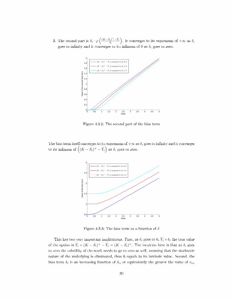
2. The second part is δi · ϕ(
(K−Si)+−Yiδi
). It converges to its supremum of +∞ as δi
goes to innity and it converges to its inmum of 0 as δi goes to zero.
0 0.5 1 1.5 2 2.5 3 3.5 4 4.5 50
0.2
0.4
0.6
0.8
1
1.2
1.4
1.6
1.8
2
Delta
Val
ue o
f the
sec
ond
bias
term
(K − Si)+ − Yi is assumed to be 0.5
(K − Si)+ − Yi is assumed to be 1.0
(K − Si)+ − Yi is assumed to be 1.5
Figure 4.3.2: The second part of the bias term
The bias term itself converges to its supremum of +∞ as δi goes to innity and it converges
to its inmum of(
(K − Si)+ − Yi)as δi goes to zero.
0 0.5 1 1.5 2 2.5 3 3.5 4 4.5 50.5
1
1.5
2
2.5
3
Delta
Val
ue o
f the
bia
s te
rm
(K − Si)+ − Yi is assumed to be 0.5
(K − Si)+ − Yi is assumed to be 1.0
(K − Si)+ − Yi is assumed to be 1.5
Figure 4.3.3: The bias term as a function of δ
This has two very important implications. First, as δi goes to 0, Yi + bi the true value
of the option is Yi + (K − Si)+ − Yi = (K − Si)+. The intuition here is that as δi goes
to zero the volatility of the stock needs to go to zero as well, meaning that the stochastic
nature of the underlying is eliminated, thus it equals to its intrinsic value. Second, the
bias term bi is an increasing function of δi, or equivalently the greater the value of vii,
30

the greater the bias term. Once again, vii is large if the trajectory is far removed from
the bulk of the cases, or in other words if it is biased. This implies that bi is large if
the trajectory is biased and small otherwise. Using bias free estimation of the stopping
policy, the condition for exercise is:
(K − Si)+ ≥ Yi + bi
this will less likely to hold on biased, extreme paths because the bias bi is large since
vii is big as well on these trajectories, hence implying no exercise. Given the backward
nature of LSM, this will delay the exercise, meaning that the investor will only exercise
at an earlier point in time, when the underlying's spot price is lower and thus the extra
premium of the foresight bias is eliminated from the price of the American option.
4.4 Implementation of the new approach
I was using Matlab R2010a for implementing and testing LSM algorithm and the
analytic bias correction method. The program starts with identifying the initial values
for the simulation along with preallocation of the variables used in the code. For simplicity,
I assumed 0% interest rate and chose the volatility parameter σ to be 0.2. The initial
value of the stock is 100 and there are 50 trading events in a 1 year time frame:
1 tic %starting a timer
2 r = 0; %interest rate
3 volatility = .2; %volatility
4 s_0 = 100; %price of the underlying at time 0
5 strike = 100; %strike
6 numberofpaths = 5000; %number of paths
7 N = 50; %number of exercise times
8
9 %preallocation of the below vectors and matrices
10 cashflow = zeros(numberofpaths,1);
11 residual = zeros(numberofpaths,1);
12 error = zeros(numberofpaths,1);
13 residualvar = zeros(numberofpaths,1);
14 errorvar = zeros(numberofpaths,1);
15 X = zeros(numberofpaths,3);
16 W = zeros(numberofpaths,N);
After initialization, for tractability purposes a seed is specied for the random number
generation, this means that the program will generate the same random numbers, hence
dierent algorithms are comparable since they can run on the same random paths. Monte
Carlo simulation is done by evaluating the formula of the Geometric Brownian motion s_t
31

using the randomly generated normal variables stored in the vector increments. Each
row of the matrix W is one trajectory generated by the simulation:
1 randn('seed',0) %to use seed 0
2 t=1:N; %N exercise events
3 time=t/N; %normalising the time frame to 1 year
4 s_t(:,1)=s_0*ones(numberofpaths,1);
5 dt=1/N;
6
7 for i=1:N;
8 increments = randn(numberofpaths,1);
9 s_t(:,i+1) = s_t(:,i) .* exp((r−.5 * volatility^2) * dt + volatility ...
* sqrt(dt) * increments);
10 W(:,i+1) = s_t(:,i+1);
11 end
12 W(:,1)=[];
The algorithm starts with identifying the intrinsic value at maturity on each path, par-
ticularly for a put this is done by the following. Let me note that since European options
are only exercisable at maturity, this information alone is sucient to approximate the
European option value, this is stored in the variable european_value.
1 for i=1:numberofpaths
2 if W(i,N)<strike
3 cashflow(i) = (strike − W(i,N)) * exp(−r/N);4 else
5 cashflow(i) = 0;
6 end
7 end
8
9 european_value = sum(cashflow(1:numberofpaths))/numberofpaths;
Now that the exercise policy at maturity is known, the implementation of the recursion
part of LSM is next. Working backwards for each j = N − 1, . . . , 1, in other words at
each trading event, variable index stores the indices of all the in-the-money paths. The
spot price on these trajectories are used to evaluate the regressor function and these
gures are stored in the rows of the matrix X. This is then used to calculate the variable
conditionalexp which is the regression value, the approximation of continuation.
1 for j = N−1:−1:12 index = find(strike − W(:,j) > 0); %
3 X = [ones(size(index)) W(index,j) W(index,j).^2]; %
4 B = (X'*X)\X'*cashflow(index); %B = inv(X'*X)*X'*cashflow(index);
5 conditionalexp = X * B;
32

Up until this point the algorithm is same for LSM and the new method. The following
section will calculate the bias term based on the six steps introduced in Section 4.2. The
only diculty might arise is the calculation of the error term ε = (I−V )−1 ·r, the problemis that (I − V )−1 might be badly scaled or close to be singular. Therefore, instead of
using the built in inverse function of Matlab, I used the Taylor series to calculate the
inverse, specically it is known that:
1
1− x = 1 + x+ x2 + . . . for |x| < 1
This also holds true for matrices, numerical tests suggested that even I+V gives accurate
results for the inverse of I − V .
1 %bias correction
2 V = X / (X'*X) * X'; %V = X*inv(X'*X)*X';
3 residual = cashflow(index) − conditionalexp;
4 error = (eye(size(index,1)) + V) * residual; %inv(I−V)*r5 errorvar = sum(error.^2) / size(index,1);
6 delta = sqrt(diag(V) .* errorvar);
7 b1 = (max(strike − W(index,j),0) − conditionalexp) .* ...
normcdf((max(strike − W(index,j),0) − conditionalexp) ./ delta)
8 b2 = delta .* normpdf((max(strike − W(index,j),0) − conditionalexp) ...
./ delta);
9 bias = b1 + b2;
Now that the bias term is known, it is possible to derive the stopping policy by:
1 for i = 1:size(index,1)
2 if conditionalexp(i) + bias(i) <= strike − W(index(i),j)
3 cashflow(index(i)) = (strike − W(index(i),j));
4 end
5 end
6 end
7
8 cashflow = cashflow * exp(−r/N);9 toc
10 american_value = sum(cashflow(1:numberofpaths))/numberofpaths;
At last, the value of the American option is calculated with analytic foresight bias cor-
rection method and it is stored in the variable american_value. In case the conditional
expectation is not cleaned from the look ahead bias, the exercise policy is reduced to:
33

1 for i = 1:size(index,1)
2 if conditionalexp(i) <= strike − W(index(i),j)
3 cashflow(index(i)) = (strike − W(index(i),j));
4 end
5 end
6 end
Hence, the algorithm simplies to the original method introduced by Longsta and
Schwartz.
4.5 Testing of the new approach
In this section I am going to compare the three introduced methods, namely the
original LSM, the independent path algorithm and the analytic bias correction method.
The main objective is to see if the price calculated by the analytic bias correction method
is in the optimal range. Since LSM algorithm always results in a value greater than the
theoretical price and on the other hand the independent path method is known to be
suboptimal, it is a natural requirement for the new method to compute option prices in
this optimal range. In the chart below, the y − axis represents the value of the option
whereas the x− axis shows the number of paths.
500 1000 1500 2000 2500 3000 3500 40007.7
7.8
7.9
8
8.1
8.2
8.3
8.4
Number of simulated paths
Val
ue o
f the
opt
ion
LSM algorithmAnalytic bias correctionIndependent path methodBOMP
Figure 4.5.1: Analytic bias correction test 1
The value determined by the new method is clearly in the optimal range and it seems
to uctuate a lot less then the other two methods. The next chart shows the same test;
however, this time four basis functions are used instead of three.
34

500 1000 1500 2000 2500 3000 3500 40007.8
7.9
8
8.1
8.2
8.3
8.4
Number of simulated paths
Val
ue o
f the
opt
ion
LSM algorithmAnalytic bias correctionIndependent path methodBOPM
Figure 4.5.2: Analytic bias correction test 2
The last test for the optimal range uses three basis functions; however, this time
variance of the underlying is 0.4 instead of 0.2 as in the previous two examples.
500 1000 1500 2000 2500 3000 3500 400015.5
15.6
15.7
15.8
15.9
16
16.1
16.2
16.3
16.4
Number of simelated path
Val
ue o
f the
opt
ion
LSM algorithmAnalytic bias correctionIndependent path methodBOPM
Figure 4.5.3: Analytic bias correction test 3
The option prices generated by the analytic bias correction method are in the optimal
range for all the test cases.
4.6 Areas of further research
The new method possesses the most important qualities required from any American
style contingent claim pricing model. Since it is fundamentally based on LSM algorithm,
it is exible and easy to implement because it only consists of six simple additional
steps. Moreover, it does address the look ahead bias of the original algorithm, hence it
derives a more reliable estimate of the real American option value. Even though, the
35

analytic bias removal method uses large matrices, for instance the hat matrix V , it is still
computationally tractable; however, simulations with large number of paths might be very
time and memory consuming. One possible solution to avoid dealing with large matrices is
to divide the in-the-money paths into buckets and then calculate the bias in these various
buckets. Since the number of elements of V is the square of the number of in-the-money
paths, using the bucket method will substantially reduce the size of the matrices used to
calculate the bias. Broadie and Glasserman [2004] propose a new idea called policy xing,
meaning that the investor only considers exercising if the immediate payo is greater than
a threshold. A natural choice for this threshold is the current European option price of
the underlying security. Using this approach reduces the range over which bias has to be
calculated. In addition, I conjecture that buckets close to strike or alternatively close to
the threshold will tend to be very low biased since they are not removed from the bulk of
the cases; consequently, calculating the bias term might be avoided for these particular
bins altogether. These methods further trim the size of matrix V , resulting the algorithm
to be time-wise competitive as well, even for simulations with higher number of paths.
The analytic bias correction method is now proved to be a reliable algorithm for
pricing of American call and put options. Further areas of research include testings on
derivatives with dierent and possibly more complex payos.
36

Chapter 5
Conclusion
One of the most popular areas of quantitative nance is the ongoing struggle to de-
termine the optimal exercise strategy used for the pricing of American style contingent
claims. Deriving the best exercise policy is the common goal of investors, hedge funds
and investment banks to ultimately maximize their prot. Monte Carlo simulation meth-
ods are more and more popular in derivative pricing as a result of rapid development of
computational eciency and stochastic calculus. LSM algorithm introduced by Longsta
and Schwartz is a simple yet powerful method for valuing American options. The goal of
my thesis was to gain a deep understanding of the algorithm itself along with its strengths
and weaknesses and then to address the issue of the embedded foresight bias.
The fundamental incentive was to examine the underlying least squares regression
model and furthermore to derive the distributional properties of residuals and theoreti-
cal errors. A sound understanding of these principles enabled me to reveal an unbiased
approximation of the theoretical conditional expectation value of continuation. Conse-
quently, I introduced a six-step methodology for path-wise calculation of the bias term,
a new approach for eliminating the foresight of the original algorithm. The analytic bias
removal method fullls all the natural requirements one might have towards any Amer-
ican option pricing algorithm and upon further testings it proved to be a reliable and
accurate new model.
37

Appendix A
Implementations
Implementation 1:
LSM algorithm:
1 clear all
2 tic r = 0; %interest rate
3 volatility = .2; %volatility
4 s_0 = 100; %price of the underlying at time 0
5 strike = 100;
6 numberofpaths = 1000000;
7 testnum=100;
8 N = 50; %number of the standard normals ~ number of trading events
9
10 european_value = zeros(1,testnum);
11 american_value = zeros(2,testnum);
12 cashflow = zeros(numberofpaths,1);
13
14 randn('seed',100) %to use seed 100
15
16 for g = 1:testnum
17 t = 1:N;
18 time = t/N;
19 W(:,1) = s_0*ones(numberofpaths,1);
20 dt = 1/N;
21 for i=1:N;
22 disp = randn(numberofpaths,1); %increments
23 W(:,i+1) = W(:,i) .* exp((r − 0.5 * volatility^2) * dt + ...
volatility * sqrt(dt) * disp);
24 end
25 W(:,1) = [];
26
27 for i = 1:numberofpaths
28 if W(i,N) < strike
38

29 cashflow(i) = (strike − W(i,N)) * exp(−r * dt);
30 else
31 cashflow(i) = 0;
32 end
33 end
34
35 european_value(g) = sum(cashflow(1:numberofpaths)) / numberofpaths;
36
37 for j = N−1:−1:138 index = find(strike−W(:,j) > 0);
39 X = [ones(size(index)) W(index,j) W(index,j).^2];
40 B = inv(X'*X) * X' * cashflow(index);
41 conditionalexp = X * B;
42
43 for i=1:size(index,1)
44 if conditionalexp(i) <= strike − W(index(i),j)
45 cashflow(index(i)) = (strike − W(index(i),j));
46 end
47 end
48 cashflow = cashflow * exp(−r * dt);
49 end
50 american_value(:,g) = [mean(cashflow) std(cashflow)/sqrt(numberofpaths)];
51 toc
52 end
53 american_value' european_value(:);
54 mean(american_value')
Implementation 2:
Independent path method:
1 clear all
2 tic r = 0; %interest rate
3 volatility = .2; %volatility
4 s_0 = 100; %price of the underlying at time 0
5 strike = 100;
6 numberofpaths = 5000;
7 N = 50; %number of the standard normals ~ number of trading events
8 testnum = 100;
9
10 american_value = zeros(2,testnum);
11 randn('seed',100) %to use seed 100
12
13 for g = 1:testnum
14 t = 1:N;
15 time = t/N;
16 cashflow = zeros(numberofpaths,1);
17 cashflowS = zeros(numberofpaths,1);
18 W = zeros(numberofpaths,N);
19 WS = zeros(numberofpaths,N);
39

20
21 W(:,1) = s_0 * ones(numberofpaths,1);
22 dt = 1 / N;
23 for i = 1:N;
24 disp = randn(numberofpaths,1); %increments
25 W(:,i+1) = W(:,i) .* exp((r − 0.5 * volatility^2) * dt + ...
volatility * sqrt(dt) * disp);
26 end
27 W(:,1) = [];
28
29 for i = 1:numberofpaths
30 if W(i,N) < strike
31 cashflow(i) = (strike − W(i,N)) * exp(−r * dt);
32 else
33 cashflow(i) = 0;
34 end
35 end
36
37 european_value = sum(cashflow(1:numberofpaths))/numberofpaths;
38
39 WS(:,1) = s_0 * ones(numberofpaths,1);
40 dt = 1/N;
41 for i = 1:N;
42 disp = randn(numberofpaths,1); %increments
43 WS(:,i+1) = WS(:,i) .* exp((r − 0.5 * volatility^2) * dt + ...
volatility * sqrt(dt) * disp);
44 end
45 WS(:,1) = [];
46
47 for i = 1:numberofpaths
48 if WS(i,N) < strike
49 cashflowS(i) = (strike − WS(i,N)) * exp(−r * dt);
50 else
51 cashflowS(i) = 0;
52 end
53 end
54
55 european_valueS = sum(cashflowS(1:numberofpaths))/numberofpaths;
56
57 for j = N−1:−1:158 index = find(strike − W(:,j) > 0);
59 X = [ones(size(index)) W(index,j) W(index,j).^2];
60 B = inv(X'*X) * X' * cashflow(index);
61 conditionalexp = X * B;
62
63 for i = 1:size(index,1)
64 if conditionalexp(i) <= strike − W(index(i),j)
65 cashflow(index(i)) = (strike − W(index(i),j));
66 end
67 end
40
68
69 indexS = find(strike − WS(:,j) > 0);
70 XS = [ones(size(indexS)) WS(indexS,j) WS(indexS,j).^2];
71 conditionalexpS = XS * B;
72
73 for i = 1:size(indexS,1)
74 if conditionalexpS(i) <= strike − WS(indexS(i),j)
75 cashflowS(indexS(i)) = (strike − WS(indexS(i),j));
76 end
77 end
78 cashflow = cashflow * exp(−r * dt);
79 cashflowS = cashflowS * exp(−r * dt);
80 end
81 american_value(:,g) = [mean(cashflowS) ...
std(cashflowS)/sqrt(numberofpaths)];
82 toc
83 end
84
85 american_value'
86 european_valueS(:); mean(american_value')
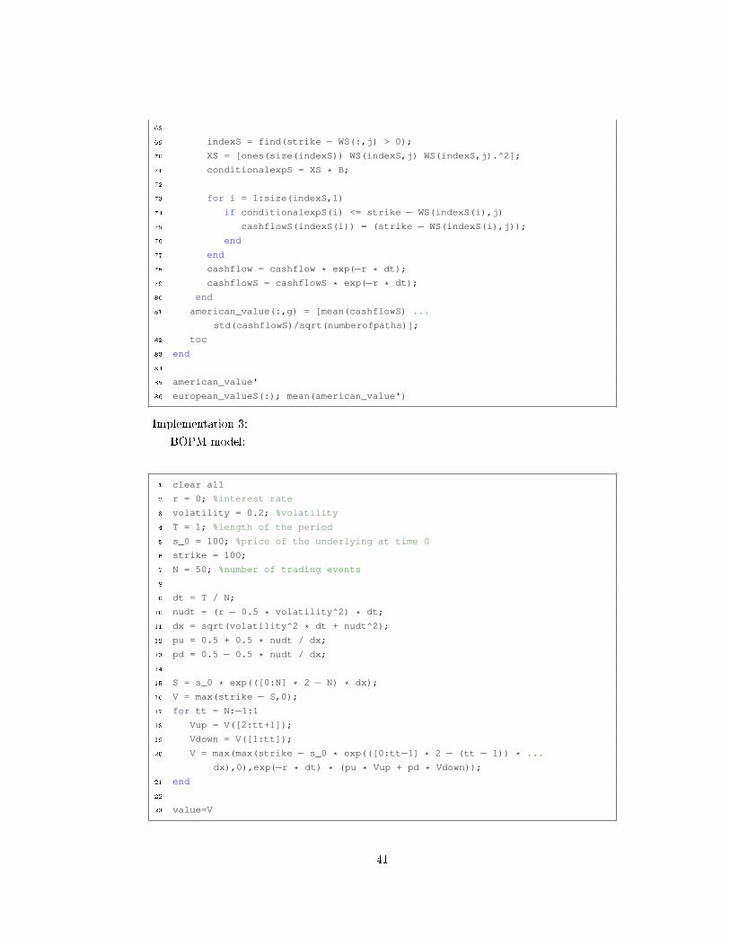
Implementation 3:
BOPM model:
1 clear all
2 r = 0; %interest rate
3 volatility = 0.2; %volatility
4 T = 1; %length of the period
5 s_0 = 100; %price of the underlying at time 0
6 strike = 100;
7 N = 50; %number of trading events
8
9 dt = T / N;
10 nudt = (r − 0.5 * volatility^2) * dt;
11 dx = sqrt(volatility^2 * dt + nudt^2);
12 pu = 0.5 + 0.5 * nudt / dx;
13 pd = 0.5 − 0.5 * nudt / dx;
14
15 S = s_0 * exp(([0:N] * 2 − N) * dx);
16 V = max(strike − S,0);
17 for tt = N:−1:118 Vup = V([2:tt+1]);
19 Vdown = V([1:tt]);
20 V = max(max(strike − s_0 * exp(([0:tt−1] * 2 − (tt − 1)) * ...
dx),0),exp(−r * dt) * (pu * Vup + pd * Vdown));
21 end
22
23 value=V
41

Appendix B
Figures
Figure 3.6.1:
Parameter of the simulation are:
1 r = 0; %interest rate
2 volatility = .2; %volatility
3 s_0 = 100; %price of the underlying at time 0
4 strike = 110; %the strike is 100
5 numberofpaths = 11;
6 N = 50; %number of the standard normals ~ number of trading events
7 randn('seed',0) %used seed 0 to generate these paths
The equation of the exercise boundary is: f(x) = 2 ·√N − x+ 110
Figure 3.6.2:
Shows the average of the means and variance of 100 re-simulations of LSM algorithm
with the below parameters:
1 r = 0; %interest rate
2 volatility = .2; %volatility
3 s_0 = 100; %price of the underlying at time 0
4 strike = 100; %the strike is 100
5 N = 50; %number of the standard normals ~ number of trading events
6 randn('seed',100) %used seed 100 to generate these paths
42

Figure 3.6.3:
Shows the average of the means and variance of 100 re-simulations of independent
path method with the below parameters:
1 r = 0; %interest rate
2 volatility = .2; %volatility
3 s_0 = 100; %price of the underlying at time 0
4 strike = 100; %the strike is 100
5 N = 50; %number of the standard normals ~ number of trading events
6 randn('seed',100) %used seed 100 to generate these paths
Let me further note that half of the indicated number of paths were used to create the
stopping rule and the remaining half were used to calculate the option price.
Figure 3.6.4:
Shows the average of the means and variance of 100 re-simulations of LSM algorithm
and independent path method with the below parameters:
1 r = 0; %interest rate
2 volatility = .2; %volatility
3 s_0 = 100; %price of the underlying at time 0
4 strike = 100; %the strike is 100
5 N = 50; %number of the standard normals ~ number of trading events
6 randn('seed',100) %used seed 100 to generate these paths
Let me further note that for the independent path method half of the indicated number of
paths were used to create the stopping rule and the remaining half were used to calculate
the option price.
Figure 4.5.1:
Shows the average of the means 100 re-simulations of LSM algorithm, analytic bias
correction method and independent path method with the below parameters:
1 r = 0; %interest rate
2 volatility = .2; %volatility
3 s_0 = 100; %price of the underlying at time 0
4 strike = 100; %the strike is 100
5 N = 50; %number of the standard normals ~ number of trading events
6 randn('seed',100) %used seed 100 to generate these paths
Let me further note that for the independent path method half of the indicated number of
paths were used to create the stopping rule and the remaining half were used to calculate
the option price.
43

Figure 4.5.2:
Shows the average of the means 100 re-simulations of LSM algorithm, analytic bias
correction method and independent path method with the same parameters as gure 9,
but 4 basis functions were used instead of 3.
Figure 4.5.3:
Shows the average of the means 100 re-simulations of LSM algorithm, analytic bias
correction method and independent path method with the below parameters:
1 r = 0; %interest rate
2 volatility = .4; %volatility
3 s_0 = 100; %price of the underlying at time 0
4 strike = 100; %the strike is 100
5 N = 50; %number of the standard normals ~ number of trading events
6 randn('seed',100) %used seed 100 to generate these paths
Let me further note that for the independent path method half of the indicated number of
paths were used to create the stopping rule and the remaining half were used to calculate
the option price.
44

Bibliography
Takeshi Amemiya. Advanced Econometrics. Harvard University Press, 1985.
Alain Bensoussan. On the theory of option pricing. Acta Applicandae Mathematicae, 2,
1984.
Fisher Black and Myron Scholes. The pricing of options and corporate liabilities. The
Jornual of Political Economy, 81, 1973.
Mark Broadie and Paul Glasserman. A stochastic mesh method for pricing high-
dimensional american options. Journal of Computational Finance, 7, 2004.
Dennis Cook and Sanford Weisberg. Characterizations of an empirical inuence function
for detecting inuential cases in regression. Technometrics, 22, 1980.
Dennis Cook and Sanford Weisberg. Monographs on Statistics and Applied Probability.
1982.
Christian Fries. The foresight bias in monte-carlo pricing of options with early exercise:
Classication, calculation & removal. 2005. URL www.christian-fries.de.
John Hull. Options, Futures and Other Derivatives. Prentice Hall, 2011.
Kiyoshi Ito. On stochastic dierential equations. American Mathematical Society, 1951.
Kenneth Judd. Numerical methods in economics. MIT Press: Cambridge, 1998.
Ioannis Karatzas. On the pricing of american options. Applied Mathematics and Opti-
mization, 17, 1988.
Francis Longsta and Eduardo Schwartz. Valuing american options by simulation: A
simple least-squares approach. Review of Financial Studies, 14, 2001.
Steven Shreve. Stochastic Calculus for Finance II: Continuous-Time Models. Springer
Finance, 2004.
Halbert White. Asymptotic Theory for Econometricians. Academic Press, 1984.
45


