Eotvos Lorand University

Faculty of Science

Gabor Meszaros

Mathematician MSc

Configurations inNon-Desarguesian Planes

Master’s Thesis

supervisor:

Tamas Szonyi, Professor

Budapest, 2011.

Contents

1. Introduction 4

2 Desarguesian Planes 6

2.1 Basic Definitions . . . . . . . . . . . . . . . . . . . . . . . . . . . . . 6

2.2 Planes Coordinatized with Fields and Skewfields . . . . . . . . . . . . 7

2.3 Desargues Theorem and Desarguesian Planes . . . . . . . . . . . . . . 9

3 Nondesarguesian Planes 12

3.1 An Elementary Method . . . . . . . . . . . . . . . . . . . . . . . . . . 12

3.2 Affine Planes Built on Nearfields . . . . . . . . . . . . . . . . . . . . 15

3.3 Hall Planes . . . . . . . . . . . . . . . . . . . . . . . . . . . . . . . . 17

4 Configurations in Desarguesian and Nondesarguesian Planes 20

4.1 Arcs, Ovals, Blocking Sets . . . . . . . . . . . . . . . . . . . . . . . . 20

4.2 Configurations in PG(2, q) . . . . . . . . . . . . . . . . . . . . . . . . 23

4.2.1 Arcs and Ovals . . . . . . . . . . . . . . . . . . . . . . . . . . 23

4.2.2 Blocking Sets . . . . . . . . . . . . . . . . . . . . . . . . . . . 24

4.3 Configurations in Hall Planes . . . . . . . . . . . . . . . . . . . . . . 26

4.3.1 Ovals in Hall(q2) . . . . . . . . . . . . . . . . . . . . . . . . . 26

4.3.2 Blocking Sets in DAG(2, q2) . . . . . . . . . . . . . . . . . . . 33

4.4 Configurations in Planes Built on Nearfields . . . . . . . . . . . . . . 34

2

Bevezetes

A projektıv sıkok absztrakt tanulmanyozasa a XIX. szazad elso feleben, J.-V. Pon-

celet es K. von Staudt munkassagaval vette kezdetet. A geometria axiomatikus

megalapozasa a mult szazad elejen, tobb neves matematikus, koztuk G. Fano, D.

Hilbert es M. Hall kozremukodesevel szuletett meg. Szinten ez ido tajt fektettek le a

sıkok algebrai eszkozokkel valo tanulmanyozasanak es a gorbeelmeletnek az alapjait.

Ezen alapokon szamos napjainkban is nepszeru matematikai terulet (peldaul lgebrai

geometria) nyugszik.

Az algebrai megkozelıtes segıtsegevel lehetove valt a sıkok behatobb tanulmanyo-

zasa es osztalyozasa. Kiemelt jelentoseggel bır e teren Hilbert 1923-as eredmenye

Desarguesi-sıkok karakterizalasarol, mely a nem-desarguesi sıkok vizsgalataban is

merfoldkonek szamıt.

Dolgozatom elsodleges celja klasszikus nem-desarguesi sıkok bemutatasa es e-

lemzese. Desargues teteletol indulva targyalunk desarguesi es nem desarguesi affin

es projektıv sıkokat. Bar a dolgozat tobb vegtelen sıkon is emlıt, erdeklodesunk

kozeppontjaban fokent veges sıkok allnak. A konstrukciok ismerteteset kovetoen

kulonfele veges geometriai strukturak — ıvek es lefogo ponthalmazok— vizsgalataba

kezdunk.

Dolgozatomban a kovetkezo tartalmi tagolast kovetem:

• Bevezetes.

• A masodik fejezet roviden osszefoglalja a testtel koordinatazott affin es pro-

jektıv sıkokkal, Desargues tetellel es desarguesi sıkokkal kapcsolatos alapveto

definıciokat es osszefuggeseket.

• A harmadik fejezetben tobb klasszikus peldat mutatunk nem-desarguesi sıkokra.

A konstrukciok ismertetese soran a szukseges algebrai fogalmak (planaris fugg-

venyek, majdnemtestek) is attekintesre kerulnek.

• A negyedik fejezetben felidezzuk az ıvekkel, ovalisokkal, lefogo- es blokkolohal-

mazokkal kapcsolatos definıciokat. Ismertetjuk a testre epıtett sıkokra vonat-

kozo eredmenyeket es belatjuk, hogy a kozolt tetelek nem vihetoek at tet-

szoleges sıkra. Kulon alfejezetet szentelunk Hall sıkok orokolt ıveinek tanul-

manyozasara, betekintest engedve az orokolt ıvek karakterizaciojanak jelenlegi

allapotaba. A meg megoldatlan reszesetek egyiket elemezve egy lehetseges

megoldasi tervet vazolunk fel. A dolgozatot Hall sıkok lefogo ponthalmazira

vonatkozo megjegyzesekkel zarjuk.

3

Configurations in Non-desarguesian Planes

Gabor Meszaros

Eotvos Lorand University, Budapest, Hungary

1. Introduction

The abstract study of projective geometry first arose in the work of J.-V. Poncelet

and K. von Staudt in the first part of the nineteenth century. About 100 years

ago, axiomatic frameworks were developed by several people, including G. Fano,

D. Hilbert, and M. Hall. In the same decades the idea of examining affine and

projective planes by using algebraic methods had been settled. The early results

about coordinatization of planes and examination of curves are counted as sources

of many even nowadays popular fields such as algebraic geometry.

In 1923, Hilbert published his landmark result about characterization of Desar-

guesian-planes. The proof of the theorem is based on algebraic methods and has

made a remarkable contribution to the study of non-desarguesian planes.

The first objective in this thesis is to introduce and study a handful of classical

non-desarguesian planes. After recalling some basic definitions and results we will

turn to the study of Desargues theorem, desarguesian and non-desarguesian affine

and projective planes. Although this thesis mentions infinite planes several times we

will mainly focus on finite planes. We will discuss classical constructions achieved in

different ways and study various finite geometric structures such as arcs and blocking

sets of the introduced planes.

Throughout my thesis the different topics mentioned above will be discussed in

the following order:

• Section 1 will cover Introduction.

• Section 2 will briefly summarize the basic definitions and theorems concerning

affine and projective planes coordinatized with fields, Desargues theorem and

desarguesian- planes as well.

• In Section 3 we will give classical examples of non-desarguesian projective

planes. While introducing various constructions we will briefly discuss the

involved algebraic structures such as planar functions and nearfields.

4

• Section 4 mainly deals with arcs, ovals and blocking sets in the previously

discussed planes. After recalling basic definitions and results we will discuss a

handful of known theorems concerning ovals and blocking sets of planes built

on finite fields and prove that the discussed theorems cannot be extended to

arbitrary planes. We will study inherited arcs in Hall-planes in details provid-

ing an insight to the current stage of the (still uncomplete) characterization

of inherited arcs. A possible (rather technical) way — which may be able to

solve some of the uncomplete cases — including demanding computations is

also introduced in this section. Finally, we will make a few remarks concerning

blocking sets of the Hall plane.

5

2 Desarguesian Planes

2.1 Basic Definitions

For further use we recall the definitions of affine and projective planes.

Definition 1 An affine plane A is a set, the elements of which are called points,

together with a collection of subsets, called lines, satisfying the following three ax-

ioms.

A1. For every two different points there is a unique line containing them.

A2. For every line l and a point P not in l, there is a unique line containing P

and disjoint from l.

A3. There are three points such that no line contains all three of them.

Definition 2 A projective plane is a set, the elements of which are called points,

together with a collection of subsets, called lines, satisfying the following three ax-

ioms.

P1. Any two distinct points belong to exactly one line.

P2. Any two distinct lines intersect in exactly one point.

P3. There are four points such that no line contains any three of them.

Two lines are called parallel if they are equal or disjoint. Certainly, it is an

equivalence-relation on the lines (transitivity follows from A2.) the equivalence

classes are called parallel classes. Two affine planes A,A′ (or two projective planes

P,P′) are isomorphic if there is a bijection A→ A′ (P→ P′) taking lines to lines.

Recall that a finite projective plane has t2 + t + 1 points and t2 + t + 1 lines,

each line contains t + 1 points and each point is contained by t + 1 lines, where

t ∈ N, t ≥ 2 is called the order of the plane. The notation Πq generally refers to an

arbitrary projective plane of order q.

A projective plane can be considered as a closure of a suitable affine plane. That

is, we extend the affine plane by giving additional points, called ideal points, each

of which corresponds to a parallel class and is contained by the lines in the corre-

sponding class. Furthermore we define a line, called ideal line (or line at infinity),

which contains exactly the ideal points.

6

Figure 1: Projective closure

It is easy to see that the structure given in Figure 1. satisfies the axioms

P1, P2, P3 and therefore is a projective plane. One can also define a reverse trans-

formation which yields an affine plane by deleting an arbitrary line with its points

in a projective plane. As a result, we get that a finite affine plane has t2 points and

t2 + t lines, each line contains t points and each point is contained by t+ 1 lines. We

define the order in case of affine planes as the order of their closure.

2.2 Planes Coordinatized with Fields and Skewfields

We briefly recall the definitions of affine and projective planes coordinatized with

fields and skewfields. Throughout this thesis — if we do not define it differently —

p is a positive prime and q is a positive power of p. The notation F generally refers

to an arbitrary field. We denote Fq = GF (q) that is, the Galois field of order q. In

Section 4 we also use the notation F = Fq and K = Fq2 .

The affine plane coordinatized with F is defined as the elements of F×F as points,

with the subsets — as lines — of the following forms: {(x, y) : y = m · x + b} and

{(x, y) : x = b} for all m, b ∈ F. In case of skewfields the same definition is valid.

However, the famous theorem due to Wedderburn (usually called ”Wedderburn’s

little theorem”) characterizes the finite skewfields as being fields. Since we mainly

focus on planes coordinatized with finite structures, it is sufficient to concentrate on

planes which are coordinatized with fields. We denote the affine plane arisen by the

field F with AG(2,F). Furthermore, if our field is a Galois field of order q we use

the notation AG(2, q).

By defining the projective plane coordinatized with F, a classical way is to asso-

ciate it to the three-dimensional vectorspace V over F. We define the relation ∼ in

V \{0} = F3\{0} on the following way: for u, v ∈ V \{0}, u ∼ v iff ∃λ ∈ F∗ : u = λ·v.

7

Easy calculation shows that ∼ is an equivalence relation. We define the point-set

of the projective plane P as F3/

∼, that is, the equivalence-classes of F3. One can

easily see that each point is associated to a one-dimensional subspace of V .

The elements of L — the set of lines — are defined as the images of the two-

dimensional subspaces of V by factoring with ∼. In other words, a subset of P is a

line iff the corresponding one-dimensional subspaces are exactly the subspaces of a

two-dimensional subspace in V .

As each two-dimensional subspace has a unique orthogonal space in V it can be

described by giving the corresponding element of this subspace in P . In this way the

elements of P and L are both uniquely coded with the elements of V \{0} up to scalar

multiplication. For the sake of simplicity we keep the convention of writing (ac, b

c, 1)

(c 6= 0), (ab, 1, 0) and (1, 0, 0) instead of (a, b, c), (a, b, 0), (a, 0, 0) ∈ P , respectively.

For the elements of L we use the notation [ac, b

c, 1] (c 6= 0), [a

b, 1, 0] and [1, 0, 0].

Note that the point (a, b, c) ∈ P is contained in the line [d, e, f ] ∈ L if and only if

〈(a, b, c), [d, e, f ]〉 = a · d+ b · e+ c · f = 0.

According to our previous remark deleting the line [0, 0, 1] with its points, we get

an affine plane with point-set P ′ = {(a, b, 1) : a, b ∈ F} and line-set L′ = {[m, 1, c] :

m, c ∈ F} ∪ {[1, 0, d] : d ∈ F}. Elementary calculation shows that the function

ϕ : P ′ → F × F, ϕ((a, b, 1)) = (a, b) is bijective and takes lines into lines, as the

images of the lines [m, 1, c] and [1, 0, d] in AG(2,F) are exactly the lines defined by

the equations y = −m·x−c and x = −d, respectively. It means that our affine plane

is isomorphic to AG(2, q). PG(2,F) denotes the projective closure of AG(2,F). In

case of Galois fields the notation PG(2, q) is used.

As we have seen there are two basic concept by coordinatizing affine planes. Ei-

ther we can use euclidean-coordinates (as we did by defining AG(2, q)) or consider

our affine plane as embedded in its projective closure and use the previously intro-

duced coordinate-triples called homogeneous coordinates. Throughout this thesis we

will not prefer either to the other and choose the one which better suits the current

goal. As the conversion between the two notations is straightforward we will not

discuss it in details.

Example 1 The graph of the function y = x2 in affine sense contains the points

{(a, a2) : a ∈ F} in AG(2,F). In projective sense, however, the same function has

the form x2 = y · z and contains the following points of PG(2,F): {(a, a2, 1) : a ∈F} ∪ {(0, 1, 0)}.

For the sake of simplicity we use the notation (0) = (0, 0, 1) and (∞) = (0, 1, 0)

whenever it is not confusing.

8

2.3 Desargues Theorem and Desarguesian Planes

The investigation of general projective planes is essentially based on the early the-

orem named after Desargues∗. To discuss the theorem a pair of definitions about

general projective planes is needed.

Definition 3 Two triangles, with their vertices named in a particular order, are

said to be perspective from a point P (or briefly, “point-perspective”) if their three

pairs of corresponding vertices are joined by concurrent lines.

Figure 2: Point-perspective triangles with respect P

Definition 4 Two triangles are said to be perspective from a line l (“line-perspective”)

if their three pairs of corresponding sides meet in collinear points.

Figure 3: Line-perspective triangles with respect l

∗Girard Desargues (1591-1661) French mathematician and engineer, considered as one of the

founders of projective geometry.

9

In affine sense the definitions need additional refinement in order to translate

the case when some of the intersections lie on the ideal line. Two triangles are also

said to be point-perspective if the corresponding lines defined by their vertices are

parallel. Two triangles are line-perspective if the pairs of corresponding sides are

pairwise parallel.

The two perspectivities are joined by the following famous theorem:

Theorem 1 (Hilbert) Let F be any field or skewfield. Two triangles are perspec-

tive from a point if and only if they are perspective from a line.†

Desargues theorem can be formulated in higher dimensional projective spaces as

well and it has been proven that in any projective space of dimension at least three

Desargues theorem is a direct consequence of the space axioms. This astonishing

result implied the natural question whether Desargues theorem can be also extended

to an arbitrary projective plane. Moulton disproved the conjecture by constructing

a projective planes and showing two triangles which do not hold Theorem 1.

Construction 1 We construct a new plane on R×R by modifying the lines which

have positive slopes. We define the images of the line y = m ·x+b (m, b ∈ R,m > 0)

as {(x, y) : y ≤ 0, y = m · x+ b} ∪ {(x, y) : y > 0, y = m2· x+ b}. In other words one

can say that the lines of positive slopes ”refract” on the x-axis.

Figure 4: Moulton plane

†Deargues theorem in the current form was first stated by Hilbert in the early years of the

nineteenth century.

10

One can easily prove the given structure holds axiom A1., A2., A3. and so is an

affine plane. To prove that Moulton’s construction yields a nondesarguesian plane

a possible example for point-perspective but not line-perspective triangles is given

below.

Figure 5: The triangles ABC and A′B′C ′ are certainly point-perspective with re-

spect P. The lines AB,AC, B′C ′ have positives slopes and so they refract on the

x-axis. It yields that AC does not meet A′C ′ on the y-axis (as it would do in

AG(2,R)) and so the intersections X, Y , Z are not collinear in the Moulton plane,

which disproves Desargues theorem.

A natural question arisen by Moulton’s construction is for which projective planes

is Theorem 1 valid. Such planes are called desarguesian. Many constructions for

nondesarguesian planes have been developed in the early years of the 20th century.

The final characterization of desarguesian planes was achieved by Hilbert.

Theorem 2 (Hilbert) A projective plane is desarguesian if and only if it can be

coordinatized with a skew-field.

Note that as a consequence of Hilbert’s theorem we get that finite desarguesian

projective planes are all isomorphic to one of the PG(2, q) planes for a suitable q.

Hilbert’s theorem also says that whenever a coordinatization of a projective plane

with a binary algebraic structure is given then the plane is desarguesian if and only

if the given algebraic structure is a skewfield (see [9] for details).

11

3 Nondesarguesian Planes

Although the first nondesarguesian planes have been explored in the late eighties of

the 19th century, it took a measurable time to invent effective methods which yield

nondesarguesian planes.

Our first goal is in this section to demonstrate that searching for non-desarguesian

planes may become a very demanding attempt. Afterwards we introduce general

and particular methods to construct nondesarguesian affine and projective planes.

Firstly, we consider a family of affine planes arisen by an elementary idea.

3.1 An Elementary Method

We define a new geometric structure on the point-set of AG(2,R) by replacing some

of the plane’s lines with other algebraic curves.

Construction 2 On the point-set P = R×R we define the set of lines as the union

of vertical lines in AG(2,R) (i.e. x = c for all c ∈ R) and the graphs of the functions

f(x) = m · x3 + b for all m, b ∈ R, that is

L = {y = c : c ∈ R} ∪ {m · x3 + b : m, b ∈ R}.

Statement 1 Π = {P ,L} satisfies A1, A2, A3 and A4 and so is an affine plane.

Proof Since the function f : R→ R, f(x) = m ·x3 + b (m, b ∈ R,m 6= 0) is bijective,

the equation-system y = m1 · x3 + b1

y = m2 · x3 + b2(1)

has a unique solution in x for m1 6= m2. It completes the proof of A1. Taking some

elementary observation one can easily prove the rest which we will not discuss in

details. �

Corollary 1 Assume f : R → R is a bijective function. We define the lines of

P = R× R as follows:

L = {y = c : c ∈ R} ∪ {m · f(x) + b : m, b ∈ R}.

In this case (P ,L) is an affine plane.

12

Statement 2 Π = {P ,L} is desarguesian. Moreover, it is isomorphic to AG(2,R).

Proof We define the function ϕ : AG(2,R) → Π, ϕ((a, b)) = (a, 3√b). Certainly, ϕ

is bijective. Since the point (a, b) is contained by the line y = m · x+ b in AG(2,R)

iff the line y = m · x3 + b in Π contains ϕ((a, b)) = (a, 3√b), ϕ takes lines into lines

and so is an isomorphism. �

Even using the more general form of our idea we get the same result, that is,

a peculiar interpretation of AG(2, q). It seems that the more complicated way of

constructing a plane does not necessarily yield the more intricate structure.

Our second idea is also based on replacing the lines of AG(2,R) with curves.

This time we introduce first a general approach.

Construction 3 Let f : R→ R be a suitable function and f ∗ ⊂ R2 the graph of f .

We redefine the set of lines in AG(2,R) as the union of vertical lines (that is, x = c

for all c ∈ R) and the translates of f ∗ with all vectors v ∈ R2. In other words,

L =⋃c∈R{(c, y) : y ∈ R} ∪

⋃a,b∈R{(x+ a, y + b) : (x, y) ∈ f ∗}.

Not surprisingly, for an arbitrary real valued function f , the associated structure

given in Construction 3 is far from being an affine plane as it may harm the axioms

A1. and A2. in many ways. To say the least, one cannot even be sure that different

translations of f ∗ yield different lines (as they usually do not, see e.g. the constant

functions).

To get an affine plane in Construction 3 a necessary and sufficient condition for

f ∗ is the following.

Theorem 3 Construction 3 yields an affine plane if and only if for each v ∈ R2, v =

(v1, v2), v1 6= 0 there exists a unique pair (P1, P2), P1, P2 ∈ f ∗ such that−−→P1P2 = v.

A function satisfying the previous property is called planar. We denote the affine

plane arisen by f with I(f). Planar functions do exist as we will see it soon. As an

example and easy exercise we state that the function f(x) = x2 is planar.

For being a planar function equivalent and sufficient but not equivalent conditions

are the following.

Theorem 4 f : R → R is planar if and only if for all a ∈ R\{0} the function

g(x) = f(x+ a)− f(x) is bijective.

Theorem 5 If the function f : R → R is strictly convex and lim−∞

f(x)x

= −∞,

lim+∞

f(x)x

= +∞ then f is planar.

13

For further equivalent conditions and additional details we refer [5].

Even having a proof that we did construct an affine plane it may occur that

our plane does not differ from those we have already mentioned. As an example we

prove it happens by choosing the function f(x) = x2.

Statement 3 The plane I(x2) is isomorphic to AG(2,R).

Proof We define the function ϕ : R2 → R2, ϕ((x, y)

)= (x, x2 + y). Certainly ϕ

is bijective. In additions

ϕ(x,m · x+ b) = (x, x2 +m · x+ b),

so the image of the line defined by the equation y = m · x + b is the set of points

satisfying the equation y = x2 + m · x + b = (x + m2

)2 + b − m2

4. It means that ϕ

maps lines into lines and so is an isomorphism. �

By Theorem 3 the function f(x) = x4 also yields an affine plane. Surprisingly the

plane I(x4) reveals essential differences comparing it with I(x2) as the former one is

not desarguesian. For the complete proof of the statement we refer [11]. A possible

construction violating Theorem 1 is given below (note that the direct calculation of

the “lines” defined by the given points may become very demanding. In [11] these

overwhelming calculations are avoided).

Construction 4 The triangles ABC and A′B′C ′ given by the points A(0;−1),

B(12;−1), C(1

2; 3) and A′(0;−2), B′(1;−2), C ′(1; 12) are line perspective but not

point-perspective.

It is a natural goal to characterize the desarguesian planes arisen by real valued

functions. Although the problem has not been solved yet in the general case, many

particular results are known.

Theorem 6 The continuous planar functions which yield desarguesian planes are

parabolas.

The examination of planarity can be also extended to functions over finite fields

which yield various intriguing constructions. As an example we mention the function

f(x) = xp+1 is planar over Fph . Moreover, for h = 2 the affine plane given by the

construction is isomorphic to AG(2, p2) while for h = 3 it yields a proper non-

desarguesian translation plane‡

For the deeper understanding of planar functions and affine planes built on them

we refer [4],[5] and [8].

‡A projective plane Πq is called translation plane with respect of the line l if for a fixed C ∈ l

and for each A, B 6∈ l there exists an elation ( a collineation fixing any point of l and mapping any

line through C onto itself ) which maps A to B. See further details about translation planes in [9].

14

3.2 Affine Planes Built on Nearfields

We are going to investigate further constructions which yield nondesarguesian planes.

As we have seen, dealing with a general non-desarguesian plane may be a very tough

attempt. Therefore we wish to use convenient algebraic structures to coordinatize

our plane. Since according to Theorem 2 planes coordinatized with fields or skew-

fields are necessarily desarguesian, we need a somehow weaker structure to succeed.

In the very early years of the 1900s Dickson had examined the independence of

field axioms. As a part of his result he presented in his paper ([6]) a nine-element

structure having two binary operations“+”and“·”, satisfying each field axiom except

(multiplicative) commutativity and right-distributivity. Two years later, Veblen and

Wedderburn constructed nondesarguesian planes using Dickson’s inventions. These

early results are counted as the main bases of the explorations of Nearfields§.

Definition 5 The set N with the binary operations + and · is called a (left) Nearfield

if the following conditions hold:

1. (N,+) is a group (with 0 as identity),

2. (N\{0}, ·) is a group,

3. a · (b+ c) = a · b+ a · c ∀a, b, c ∈ N .

One can define right nearfields in a similar way by modifying axiom 3. Through-

out this thesis we will work with left nearfields, taking a remark that as it happens

by examining rings and their opposites, one would be able to formulate the following

results using right nearfields as well.

The lack of right distributivity causes weird phenomena in our structure. As an

example, we mention that despite the case of fields 0 · a = 0 does not follow from

the axioms as it is not even true in the general case. We disprove our assumption

by introducing the unique two-element nearfield which is not isomorphic to the field

F2.

Example 2 Two-element nearfield.

+ 0 1

0 0 1

1 1 0

· 0 1

0 0 1

1 0 1

§There are even weaker algebraic structures (quasi-fields, ternary rings) which give a more

general approach to the coordinatization of planes. Since calculations in the general cases (when

multiplication is not even associative) may become very difficult, we focus on the special case when

our quasi-field is a near-field. For additional details concerning general coordinatization we refer

[9]

15

In some articles nearfields are defined automatically as being commutative (a+

b = b+ a) and null-symmetric (a · 0 = 0 · a = 0) as both conditions can be inferred

from the axioms for |N | ≥ 3 (commutativity is true even for |N | = 2). We refer [3]

for details.

We are going to discuss a classical construction which yields a “proper” nearfield

by “distorting” the multiplication in a field.

Construction 5 ¶ For an arbitrary odd prime p we define a multiplication ∗ in

Fq2 = Fp2k on the following way (recall that a ∈ Fq2 is a square-element if there

exists b ∈ Fq2 : b2 = a):

a ∗ b =

a · b if a is a square,

a · bq otherwise.(2)

Simple calculation yields that (Fq,+, ∗) is a proper nearfield. A nearfield N is

called Dickson nearfield if there is a field F such that N is isomorphic to (F,+, ∗)(∗ is the distorted multiplication of F similarly to Construction 5).

In 1930 Zassenhaus characterized nearfields showing that they are either Dickson

nearfields or belong to 8 exceptional nearfields of order 2, 52, 72, 112 (two noniso-

morphic examples), 232, 292 or 592. Hence all finite nearfields can considered to be

“known”.

Note that beside being very useful tools in the construction of nondesarguesian

planes nearfields had been proven to play essential role in the study of sharply two-

transitive permutation groups as well.

Theorem 7 ‖ If G is a sharply 2-transitive finite group then there is a nearfield

(N,+, ◦), such that G is isomorphic to the group of all transformations x→ x◦a+b.

Now we turn to the study of affine planes coordinatized with (Dickson’s type)

nearfields. Let N be a finite nearfield associated to Fq2 as described in Construction

5. We define the affine plane (P ,L) on P = N ×N with the subsets (as lines):

L =⋃

m,b∈N

{(x, y) : y = m ∗ x+ b} ∪⋃

b∈N

{(x, y) : x = b}.

¶The original construction due to Dickson is much more general, we apply it only for finite

fields.‖The theorem has a more general form concerning permutation groups of arbitrary cardinality,

in which case the theorem says that for each sharply two-transitive permutation group there exists a

”near-domain” (roughly spoken, an ”additively nonassociative nearfield”) such that G is isomorphic

to the group of the mentioned transformations.

16

We wish to state that by choosing an arbitrary (not necessarily finite) nearfield

the previously discussed construction does not necessarily yield an affine plane, as

the equation a ∗ x = b ∗ x+ b may have no unique solution (or no solution at all).

Definition 6 A (left) nearfield N is planar if the equation a ∗ x = b ∗ x + c has a

unique solution for all a, b, c ∈ N .

Although non-planar nearfields do exists, Zemmer proved that every finite nearfield

is planar. It also implies that our construction does yield an affine plane (we leave

both facts as exercises). We denote the affine plane built on the Dickson’s nearfield

(Fq,+, ∗) with∑

q if it is not confusing.

Our next goal is to prove that the given plane is not desarguesian. It can be easily

achieved either by recalling Theorem 2 or showing a configuration which violates

Theorem 1. We leave the latter way as an exercise.

Although throughout this thesis an affine plane coordinatized with a nearfield

always means Construction 5 we mention that coordinatization by using nearfields

can be made in numerous ways. A famous family of planes called Hughes-planes

reveals another example of projective planes built on nearfields. In order to show a

measurable difference between∑

q and Hughes-planes we mention without further

discussion that the latter family does not belong to the family of translation-planes

(while∑

q does).

3.3 Hall Planes

We have just seen an example for nondesarguesian planes arisen by distorting the

multiplication of a finite field. In our next example we modify the structure of the

affine plane AG(2, q) through an operation usually called derivation.

We recall that every line in AG(2, q2) contains q2 points. In addition, our plane

has subplanes of order q (also called Baer-subplane, see Section 4) which also contains

the same number of points and lines. This elementary observation had driven people

to the exploration of Hall planes.

Definition 7 Let q be an arbitrary power of an odd prime p and let l∞ = [0, 0, 1]

be a line of PG(2, q2). A derivation set D of AG(2, q2) = PG(2, q2)\l∞ is a set of

q + 1 points in l∞ such that for any two affine points P and Q for which the ideal

point of the line PQ is in D there is a Baer subplane containing P,Q and whose

ideal points coincide with D.

We define a new incidence structure DAG(2, q2) as follows: the points are the

points of AG(2, q2). A line is either a line of AG(2, q2) with ideal point not in D or

17

the points of a Baer subplane in AG(2, q2) whose ideal points coincide with D. The

incidence relation is the natural containment relation.

It can be proven by examining numerous cases that (assuming the existence of a

suitable set D) DAG(2, q2) is an affine plane of order q2. We define the Hall plane

of order q2 as the projective completion of DAG(2, q2) and denote it by Hall(q2).

Certainly, the derivation set D cannot be chosen arbitrarily as the condition

given above does not necessarily hold. Choosing the line [0, 0, 1] as l∞, however, one

can prove that the set D0 = {(1, x, 0) : x ∈ Fq} ∪ {(0, 1, 0)} is a valid derivation

set, usually called the real derivation set of AG(2, q2). Moreover it is known that

different derivation-sets yield isomorphic planes as a derivation set can be mapped

to another by using an appropriate collineation. It means that a possible way of

examining Hall planes is to fix a convenient derivation set (such as D0). However, as

we will see it soon sometimes it makes more sense to take advantages of the planes

symmetries on different ways.

The affine Baer-subplanes whose ideal points are those on D0 are the setsR(a, b, c) =

{(a · u+ b, a · v + c) : u, v ∈ Fq} for all a, b, c ∈ Fq2 , a 6= 0. Different choices of a, b, c

do not necessarily imply different lines.

Lemma 1 R(a1, b1, c1) and R(a2, b2, c2) are disjoint or coincident if and only ifa2

a1∈ Fq and are coincident iff a2

a1∈ Fq, b2−b1

a1∈ Fq and c2−c1

a1∈ Fq.

Proof If a1

a2∈ Fq then {a1 · u : u ∈ Fq} = {a2 · u : u ∈ Fq} and so R(a1, b1, c1) =

R(a2, b1, c1). Now if there exist u1, u2, v1, v2 ∈ Fq such that (a1 ·u1 +b1, a1 ·v1 +c1) =

(a1 · u2 + b2, a1 · v2 + c2) then a1 · (u1 − u2) = b2 − b1 and a1 · (v2 − v1) = c2 − c1.As a1 6= 0 it implies b2−b1

a1∈ Fq and c2−c1

a1∈ Fq. Fixing the elements u2, v2 we get in

addition that u1 = u2 + b2−b1a1

,

v1 = v2 + c2−c1a1

,(3)

which are valid solutions for u1, v1. It means if a1

a2∈ Fq and R(a1, b1, c1) ∩

R(a2, b2, c2) 6= ∅ then R(a1, b1, c1) = R(a2, b2, c2).

Conversely, R(a1, b1, c1) = R(a2, b2, c2) yields that for every there u2, v2 ∈ Fq

there exist u1, v1 ∈ Fq such that (a1 · u1 + b1, a1 · v1 + c1) = (a1 · u2 + b2, a1 · v2 + c2).

Solving the equations we get u1 = a2

a1· u2 + b2−b1

a1,

v1 = a2

a1· v2 + c2−c1

a1.

(4)

18

Choosing u2 = v2 = 0 yields b2−b1a1

, c2−c1a1∈ Fq and so a2

a1· u2,

a2

a1· v2 ∈ Fq and

therefore a2

a1∈ Fq.

The second part of the lemma follows easily from our proof.�

Statement 4 Hall(q2) is non-desarguesian plane for all q.

Proof With the appropriate choice of the coordinates the lines defined by the

given points remain lines in Hall(q2) except the one defined by X and Y which has

been converted to the real Baer subplane, no more containing Z. It certainly yields

two point-perspective but not line-perspective triangles and so harms Theorem 1.

Figure 6: Triangles violating Theorem 1 in the Hall plane

Note that although it is a nice, geometric way to define Hall planes through

derivation they were originally introduced algebraically via Hall quasifields.

Definition 8 Let f(x) = x2 − a · x− b be an irreducible quadratic polynomial over

Fq. The elements of the Hall quasifield H(s, f) are the elements a+ i · b (a, b ∈ Fq).

Addition is defined naturally, and the multiplication ◦ by the rule

(a+ i · b)◦ (a′+ i · b′) =

a · a′ + i · a · b if b = 0,

a · a′ + b−1b′f(a) + i ·(b · a′ + (1 + a) · b′

)if b 6= 0.

(5)

As we mentioned previously one can build an affine plane using ”week” algebraic

structures such as H(s, f). It can be shown that with proper choice of s and f the

affine plane is isomorphic to DAG(2, q).

Although Hall planes are not desarguesian it may happen that we have done noth-

ing but gave a reinterpretation of the previously discussed planes built on nearfields.

Fortunately it is not the case as Σq2 and Hall(q2) are non-isomorphic planes for all

q. A proof of our statement through a more general approach using quasifields is

presented in [9] which we neglect in this thesis.

19

4 Configurations in Desarguesian and Nondesar-

guesian Planes

The main goal of our previous section was to introduce a handful of classical con-

structions yielding non-desarguesian planes. In this section we analyze combinatorial

properties of the mentioned planes. First and foremost we recall the basic definitions

and result concerning arcs, ovals and blocking sets.

4.1 Arcs, Ovals, Blocking Sets

Definition 9 A k-arc in a finite projective or affine plane is a set of k points no

three of which are collinear. A k-arc is complete if it is not contained in a (k + 1)-

arc. A line L is secant, tangent or passant to an arc if they have 2,1 or 0 points in

common, respectively.

As the union of the lines defined by the points of an arc contains each point of

the plane, it implies a k-arc cannot be complete if q ≥ k·(k−1)2

. On the other hand,

a well-known theorem due to Bose says that a k-arc in a plane of order q contains

at most q + 1 points if q is odd and q + 2 if q is even. (q + 1)-arcs and (q + 2)-arcs

are called ovals and hyperovals, respectively. An oval in Πq of even order can be

uniquely completed to a hyperoval by adding a further point (the intersection of the

tangent lines) called “nucleus” of the oval.

The existence of ovals in a general plane is a famous unsolved problem. As an

early result, the ovals in PG(2, q) are fully described. Later on we will introduce

some classical constructions. Before doing so we recall some basic definitions.

Definition 10 Let K be a set of k points of an arbitrary plane Πq. A point P ∈ Kis an internal nucleus (shortly: i-nucleus) of K if every line through P meets K in

at most two points (including P ). The set of i-nuclei of K is denoted by IN(K).

Definition 11 Let H ⊂ Πq and P ∈ Π\H. P is called external point if there exists

a tangent line through P , that is, a line intersecting H in exactly one point. If no

such a line exists then P is called interior point.

Let O be an oval on Πq (q odd) and let T ∈ O an arbitrary point. Since

|O\{T}| = q and there are exactly q + 1 lines passing through T it yields O has a

unique tangent line through each of its points.

Now assume t is a tangent line (T ∈ t) and let P ∈ t\{P}. Each line l through

P meets O in at most two points, that is, |l ∩ O| ∈ {0, 1, 2}. As q is odd and t is

tangent there must exist another tangent line t′ through P .

20

Figure 7: Tangents of an oval

On the other hand O possesses q tangent lines different from t each of which

meets t in an external point. As each of the P ’s in t is contained by at least one of

those lines it yields equation holds and there exist exactly two tangent lines through

any P .

We have just proven if P is contained in a tangent line then P is an intersection

of exactly two tangents and so we proved the following lemma.

Lemma 2 Let q odd and O be an oval on Πq. There exist either 0 or 2 tangent

lines (with respect of O) through any point P 6∈ O.

Having been proven the previous lemma elementary calculation yields the number

of external and interior points.

Lemma 3 The plane Πq with the oval O has q·(q+1)2

external and q·(q−1)2

interior

points. A passant or secant line l has q+12

external points.

Proof The set of external point is covered by the q+1 tangent lines. Each of them is

uniquely defined as the intersection of two of the tangents. It means the number of

external points is(

q+12

)and so the number of internal points is q2 −

(q+12

)= q·(q−1)

2.

If the line l has k external points and meets the C in m points then the —

counting the number of tangents to C — we get q + 1 = 2 · k + m. As m = 0

(passant) or m = 2 (secant) the proof has been completed. �

Another intriguing topic in the study of finite affine and projective planes is the

examination of point-sets which meet every line in the plane.

Definition 12 The set of points B in a projective plane is called blocking set, if

does not contain a line and meets every line at least one point.

21

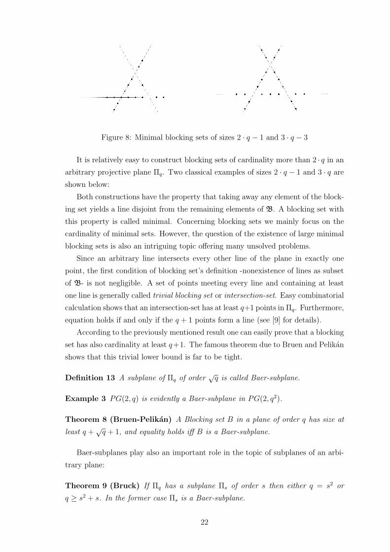
Figure 8: Minimal blocking sets of sizes 2 · q − 1 and 3 · q − 3

It is relatively easy to construct blocking sets of cardinality more than 2 · q in an

arbitrary projective plane Πq. Two classical examples of sizes 2 · q − 1 and 3 · q are

shown below:

Both constructions have the property that taking away any element of the block-

ing set yields a line disjoint from the remaining elements of B. A blocking set with

this property is called minimal. Concerning blocking sets we mainly focus on the

cardinality of minimal sets. However, the question of the existence of large minimal

blocking sets is also an intriguing topic offering many unsolved problems.

Since an arbitrary line intersects every other line of the plane in exactly one

point, the first condition of blocking set’s definition -nonexistence of lines as subset

of B- is not negligible. A set of points meeting every line and containing at least

one line is generally called trivial blocking set or intersection-set. Easy combinatorial

calculation shows that an intersection-set has at least q+1 points in Πq. Furthermore,

equation holds if and only if the q + 1 points form a line (see [9] for details).

According to the previously mentioned result one can easily prove that a blocking

set has also cardinality at least q+1. The famous theorem due to Bruen and Pelikan

shows that this trivial lower bound is far to be tight.

Definition 13 A subplane of Πq of order√q is called Baer-subplane.

Example 3 PG(2, q) is evidently a Baer-subplane in PG(2, q2).

Theorem 8 (Bruen-Pelikan) A Blocking set B in a plane of order q has size at

least q +√q + 1, and equality holds iff B is a Baer-subplane.

Baer-subplanes play also an important role in the topic of subplanes of an arbi-

trary plane:

Theorem 9 (Bruck) If Πq has a subplane Πs of order s then either q = s2 or

q ≥ s2 + s. In the former case Πs is a Baer-subplane.

22

It has been a longstanding problem whether every projective plane of order q2

has a Baer-subplane. Generally the structure of subplanes in projective planes or in

other words the embedding of projective planes is a very intriguing and diversified

field which offers challenging problems and astonishing results. As an example we

mention that while the embedding of Fano plane is straightforward to PG(2, 2h) for

each h ∈ Z+ it can be also embedded to each of the previously mentioned Hughes-

planes. In addition Caliscan and Moorhouse recently showed (in [1]) an infinite

family of Hughes-planes contanining subplanes of order 3. However, embedding of

projective planes of higher order is still a widely open problem.

One can define blocking and intersection-sets of affine planes on a similar way.

Unlike the projective case blocking sets and intersection sets of affine planes are not

distinguished as they do not show significant differences.

Certainly, an affine intersection set can be completed to an intersection set in

the projective sense by adding an arbitrary point of the ideal line. Not surprisingly

this process does not work conversely as a projective intersection set can have much

smaller cardinality in a given plane than an affine set has. In the next Section we

briefly discuss the famous theorem due to Jamison and Brouver-Schrijver concern-

ing the minimal cardinality of intersection sets in AG(2, q), which reveals essential

differences between intersection sets cardinalities in affine and projective sense.

4.2 Configurations in PG(2, q)

4.2.1 Arcs and Ovals

A landmark break-trough in the examination of the ovals in PG(2, q) was Segre’s

theorem.

Theorem 10 (Segre) The ovals of PG(2, q) (q odd) are exactly the conics over

Fq.

As the conics in PG(2, q) are “known” up to projective equivalence Segre’s the-

orem characterizes the ovals of PG(2, q) in that sense.

Theorem 11 Let C be a conic in PG(2, q) and a ∈ Fq.

1. If l∞ is secant to C then C is projective equivalent to the graph of the (affine)

function y = ax

with its ideal points.

2. If l∞ is tangent to C then C is projective equivalent to the graph of the (affine)

function y = a · x2 with its ideal points.

23

3. If l∞ is passant to C then C is projective equivalent to the graph of the (affine)

function y2 − a · x2 = 1.

Note that in case of planes of even order the characterization of ovals in PG(2, q)

is far from being completed.

Even having a general overview of the ovals of PG(2, q) for odd q complete arcs

still remain an intriguing topic. We briefly summarize a few remarkable results

concerning the possible size of a complete arc in PG(2, q).

Theorem 12 If K is a k-arc in PG(2, q) and

1. k ≥ q+42

, if q is even,

2. k ≥ 2q+53

, if q is odd,

then K is contained in a unique complete arc.

Theorem 13 (Segre) If K is a k-arc in PG(2, q) and

1. k > q −√q + 1, if q is even,

2. k > q −√

q

4+ 7

4, if q is odd,

then K can be completed to an oval.

The proof of these theorems is based on the examination of algebraic curves

associated to arcs and on Weil’s theorem. In some particular cases sharper bounds

have been proven by Voloch.

One of our main goals in the following Section is to show that the majority of

the listed theorems cannot be extended to an arbitrary projective plane.

4.2.2 Blocking Sets

There are numerous methods to construct blocking sets which we will not discuss

in details. Instead of doing so we briefly summarize the most known theorems

concerning sizes of (affine or projective) blocking sets.

Theorem 14 (Blokhuis) A blocking set B in PG(2, p) contains at least 3(p+1)2

points.

As the existence of a projective plane of order p which is not isomorphic to

PG(2, p) is a well known open problem, we are not able to analyze the result of

the theorem in case of non-desarguesian planes. However, the theorem has a more

general form due to the same author:

24

Theorem 15 (Blokhuis) Let q = pn, n ≥ 2. A blocking set B in PG(2, q) has at

least

1. q +√q + 1 points, if n is even,

2. q +√p · q + 1 points if n is odd.

Note that in the case of even n our lower bound is the same as in Theorem 8.

We mention another famous theorem concerning blocking sets of affine planes

built on fields:

Theorem 16 (Jamison,Brouwer-Schrijver) A blocking set of B in AG(2, q) con-

tains at least 2 · q − 1 points.

For the affine case a short and elegant proof has been given by the authors. The

techniques involved in the proof can be also considered as an early stage of the later

invented theorem usually known as Combinatorial-Nullstellensatz.

25

4.3 Configurations in Hall Planes

4.3.1 Ovals in Hall(q2)

Throughout this section we consider inherited arcs. An arc and especially an oval

of AG(2, q2) or PG(2, q2) is called inherited if it is also an arcs (oval) in Hall(q2).

In other words those arcs are called inherited which remain ovals after derivation.

Inherited arcs are counted as ”valuable treasures” as an arc of AG(2, q2) usually

does not remain an arc in Hall(q2). In order to illustrate it we discuss two early

theorems due to Szonyi. In [13] he has proved that the conic x · y = 1 does not

remain an arc in Hall(q2), moreover it has q2 − q + 1 internal nuclei and cannot

be completed to an oval. Besides giving an insight to the structure of arcs in Hall

planes Szonyi’s construction disproves Theorem 12 for Hall planes.

Theorem 17 (Szonyi) The set of points C defined by the function f(x) = x2 to-

gether with (∞) has q2 − q + 1 internal nuclei on Hall(q2) for odd q.

Proof As C is an arc in AG(2, q) three points cannot be contained by an old line of

DAG(2, q2). If the points (x1, x21), (x2, x

22), (x3, x

23) are on a new line, then the slopes

of the linesx2

i−x2j

xi−xj= xi + xj are in F. Since q is odd it yields x1, x2, x3 ∈ F.

It means that the set {(x, x2) : x ∈ K\F} is an arc in Hall(q2). Certainly it can

be extended with any pair of points of form (x, x2)(x ∈ F). Easy calculation shows

that by adding a pair the arc cannot be extended with any further point and so the

given points form a complete arc of size q2 − q + 2. �

Another construction due to the same author shows even weirder phenomena,

namely the existence of complete arcs which are ”almost ” ovals.

Theorem 18 (Szonyi) For an arbitrary, fixed non-square c ∈ K the hyperbola

H = {(x, −cx|0 6=∈ K)} is a complete (q2 − 1)-arc in Hall(q2).

The proof of Theorem 18 can be achieved by using similar ideas and observations

as previously discussed (see [13]).

Unlike the classical planes built on Fq2 the Hall plane does contain arcs of size

greater than q2−q which cannot be uniquely completed as we have seen in Theorem

17 and it also contains complete arcs of size greater than q2 − q + 1. It means that

neither Theorem 12 nor Theorem 13 are valid for Hall planes.

Although in the examination of arcs and ovals in the Hall planes inherited arcs

have top priority it is known that there exist ovals which are not descendant of ovals

lying in AG(2, q). A famous theorem due to Menichetti tells us that each Hall plane

of odd order does have such an oval.

26

Theorem 19 (Menichetti) In every Hall plane of even square order q2 there do

exist non-inherited complete q2-arcs.

Similar result for odd order are not known. On the contrary, it has been drawn

as a conjecture by many authors that in some particular cases (with restrictions

for the value of q) the ovals of Hall(q2) are all inherited ovals. The conjecture has

neither proved nor disproved in any part. From now on we turn our full attention

to the inherited arcs.

The characterization of inherited arcs in Hall(q2) has begun in the early eighties

and completed recently for event value of q by Cherowitzo ([2]) who finished the

work of O’Keefe, Pascasio [12] as well as Korchmaros[10] and many further authors.

A brief summary of the characterization with reference of the proofs is listed below.

Let D be an arbitrary derivation set, C is the conic, l∞ as normally. Throughout

the characterization we distinguish three main cases according to l∞ being a

I. secant line with points P and Q of the conic (hyperbolic case),

II. tangent line with point P of the conic (parabolic case),

III. an exterior line (elliptic case).

In addition we need to distinguish additional cases depending on the parity of q.

I.Hyperbolic Case

Theorem 20 [12] Suppose P,Q ∈ D.

If q = 3, then one of the following occurs:

i) The configuration of D and C is projective equivalent in AG(2, 9) to D0 and

the conic with equation x · y = 1. C is an incomplete 8 − arc in Hall(9) and

can be completed to an oval.

ii) The configuration of D and C is projective equivalent in AG(2, 9) to D0 and

the conic with equation x ·y = −d, where d is a fixed non-square in F9. In this

case C is a complete 8− arc in Hall(9).

If q > 3 odd, then one of the following occurs:

iii) The configuration of D and C is projective equivalent in AG(2, q2) to D0 and

the conic with equation x · y = 1. In this case C is not an arc in Hall(q2).

iv) The configuration of D and C is projective equivalent in AG(2, q2) to D0 and

the conic with equation x ·y = −d where d is a fixed non-square in Fq2. In this

case C is a complete (q2 − 1)-arc in Hall(q2).

27

If q > 2 even, the configuration of D and C is projective equivalent in AG(2, q2)

to D0 and the conic with equation x ·y = 1. In this case C is not an arc in Hall(q2).

Hyperbolic case, q even

Theorem 21 [2] If q > 2 is even and at least one of P and Q is not contained by

D then C is not a hyperoval in Hall(q2).

II. Parabolic case

Theorem 22 [12] If q is odd, then C is not an arc in Hall(q2).

From now on we can assume q > 2 is even. In this case the nucleus N of C lies

on l∞.

Theorem 23 [12] We distinguish three cases:

1. If P,N ∈ D then C is not an arc in DAG(2, q2).

2. If P ∈ D and N 6∈ D then the configuration of D and C is projective equivalent

in AG(2, q2) to D0 and the conic with equation y = x2 + s · x where Fq2\Fq.

In this case C is an incomplete q2-arc in DAG(2, q2) and can be completed to

a hyperoval in Hall(q2).

3. If P 6∈ D and N ∈ D then the configuration of D and C is projective equivalent

in AG(2, q2) to D0 and the conic with equation y = x2 +s ·y2 +x where Fq2\Fq.

In this case C is an incomplete q2-arc in DAG(2, q2) and can be completed to

a hyperoval in Hall(q2).

Theorem 24 [7] Any non-degenerate conic of PG(2, q2), q = 2h, with nucleus

N ∈ l∞\D and passing through a point P ∈ l∞\D, is an oval in Hall(q2) iff N and

P are conjugate points with respect to D.

III. Elliptic case, q even

Theorem 25 If q > 2 is even and l∞ does not intersect C then C is not a hyperoval

in Hall(q2).

Surveying the previously listed result we can conclude the following theorem:

Theorem 26 As a main we conclude if C is an inherited hyperoval in Hall(q2) (q

even) then it intersects the ideal line l∞ in one point.

28

As we have seen for odd q the problem is far from being fully answered. In

the following pages we are going to analyze the elliptic case and suggest a program

which offers a way to cope with the problem. We wish to state that in general cases

our path may lead us to overwhelming calculations.

Theorem 20 repetitively states that our suspected arc is projective equivalent to

a particular conic. It can be assumed without loss of generality by transforming our

point-set to a convenient conic using a suitable collineation (as it had been done in

the above mentioned papers). Recall that the collineation-group of PG(2, q) is fully

described as being a semidirect product: Coll(PG(2, q)) = PGL(2, q) o Aut(Fq).

As we have mentioned earlier we know that this group acts transitively on the sets

of possible derivation sets. It means that by analyzing a transformed conic we

can assume that our current derivation set is given as the image of D0 under a

collineation. Our goal is to gain control of the image and to investigate whether K(the set of external points in l∞) and D can be disjoint sets. In order to explain our

purpose we introduce some useful theorems due to Korchmaros.

Theorem 27 (Korchmaros) Let C be a conic and r be a line of PG(2, q) (q odd).

For every triple {P1, P2, P3} ⊂ r\C there exists at most two triangles {A1, A2, A3}inscribed in C\r such that AiAJ ∩ r ∈ {P1, P2, P3} (i 6= j, i, j = 1, 2, 3).

Theorem 28 (Korchmaros) Let C be a conic in PG(2, q) (q odd) and ABC a

triangle inscribed in C. Let r is a line containing neither of the vertices A,B,C and

let

AB ∩ r = C∗,

BC ∩ r = A∗,

CA ∩ r = B∗.

Then the set {A∗, B∗, C∗} contains either one or three external points with respect

of C.

With the choice r = l∞ we get that each inscribed triangle defines a triples in l∞,

each of which has either one or three external points. As we have(

q+12

)different

triangles and each triple is defined by at most two triangles the number of induced

triples is at least(q+1

3 )2

. On the other hand elementary combinatorial calculation

yields

∣∣∣{{P1, P2, P3} : P1, P2, P3 ∈ l∞, {P1, P2, P3} ∩ K = 1}∣∣∣ =

( q+12

2

)·( q+1

2

1

)(6)

29

∣∣∣{{P1, P2, P3} : P1, P2, P3 ∈ l∞, {P1, P2, P3} ∩ K = 3}∣∣∣ =

( q+12

3

)(7)

One can easily see(q+1

3 )2

=( q+1

22

)·( q+1

21

)+( q+1

23

)which yields each triples having

one or three external points is defined by exactly two triangles.

Now we are ready to prove our main theorem.

Theorem 29 An oval remains oval in Hall(q2) iff the derivation-set consists of no

external point.

Proof If C has collinear triples A,B,C in Hall(q2) then they are joined by a Baer-

subplane which has ideal points on l∞. According to Theorem 28 at least one of

the ideal points A∗, B∗, C∗ defined by the inscribed triangle ABC is external point

which also contained by D and so K ∩D 6= ∅.On the contrary, if D contains external point then we can complete it to a set

{P1, P2, P3} ⊂ l∞ which contains odd number of external points. Let A1, A2, A3 a

triangle associated to our triple. One can easily see that the three Baer subplanes

corresponding to the pairs {A1, A2}, {A2, A3}, {A3, A1} are identical (as each of them

contains P1,P2 and P3 as well) and so A1, A2, A3 are collinear points in Hall(q2). It

completes the proof of the theorem. �

We are going to illustrate the parametrization of the conic and the derivation

set in the elliptic case. Our goal is to get a tool which may help to decide whether

the derivation set can be disjoint from the set of external points in l∞. Let us have

an arbitrary oval of PG(2, q) which does not intersect l∞. With a proper choice of

a collineation our oval can be transformed to the ellipse C x2− k · y2 = 1 where k is

a fixed non-square in K (our derivation set D0 has been synchronously transformed

to another derivation set). Certainly the point P = (1; 0) is contained by C. Easy

calculation shows that the tangent line to C through P is the vertical line x = 1. Let

t ∈ K arbitrary element. The line of slope t through P is described by the equation

y = t · x− t and it meets C in the point Qt((

kt2+1kt2−1

; 2tkt2−1

)). The tangent line at the

point Q(x0; y0) ∈ C, Q 6= P is

y =x0

k · y0

· x− 1

k · y0

(8)

and so the tangent at Qt is

y =kt2 + 1

2kt· x− kt2 − 1

2kt(9)

which meets l∞ in the (ideal) point(1, kt2+1

2kt, 0). It yields that the set K of outer

points of C is

K = {(1, kt2 + 1

2kt, 0) : t ∈ Fq2} ∪ {(0, 1, 0)}

30

and so the set of outer points of C is parametrized with the parameter t.

Turning to the image of the derivation set we recall D0 = {(1,m, 0) : m ∈Fq} ∪ {(0, 1, 0)}. Since Fq ⊂ Fq2 is invariant under automorphisms of F 2

q hence

so is D0 as well and therefore it is sufficient to examine its image under linear

transformations.

Let A ∈ F3×3q2 be invertible matrix.

A =

a11 a12 a13

a21 a22 a23

a31 a32 a33

.

Since the line l∞ is invariant under A (as it transforms derivation set into deriva-

tion set) hence a31 = a32 = 0 can be easily concluded. As A is invertible it immedi-

ately yields a11 · a22 6= a12 · a21.

If A fixes the point (0, 1, 0) then (0, 1, 0) ∈ C∩K and so the conic does not remain

an oval. From now on we can assume A(0, 1, 0)T 6= (0, 1, 0), that is, a21 6= 0. As we

are focusing on images of ideal points the values of a13 and a23 are out of interest

and our matrix can be written in the following form:

A =

d c ∗b a ∗0 0 e

.

By the same reason as above we can assume that the equation Ax = (0, 1, 0) has

no solution in D0, which holds if and only if dc6∈ Fq.

In this case:A · (0, 1, 0)T = (c, a, 0) ∼ (1, ac, 0),

A · (1,m, 0)T = (cm+ d, am+ b, 0) ∼ (1, am+bcm+d

, 0).(10)

By denoting A = bc−adc2

, B = dc, C = a

cwe getA · (0, 1, 0) ∼ (1, C, 0),

A · (1,m, 0) ∼ (1, Am+B

+ C, 0).(11)

where A,B 6= 0, moreoverB 6∈ Fq. In addition, as B 6∈ F and K can be considered

as a quadratic extension of F: K = F(k) (k2 = d ∈ F, a non-square element) we can

assume without loss of generality that A · (1,m, 0) = (1, Am+k

+ C, 0).

Our question is whether any of the following three equations has a solution in t

and m (t ∈ K, m ∈ F) for fixed A,B,C, k parameters.

31

kt2 + 1

2kt=

A

m+ k+ C, (12)

kt2 + 1

2kt= C, (13)

1 =A

m+B+ C. (14)

Certainly (14) is easily decidable as it only depends on the given parameters.

(13) can be written in the following equivalent form: (t − C)2 = (−1) · (C2 + 1k).

This equation has a solution iff C2 + 1k

is a square in K (in particular the equation

has no solution for C = 0).

Concerning (12) a possible way is to decompose the variables in K (using the base

{1, k}) and look for solution in the components over F. We therefore reformulate

(12) introducing and using the following notation (t0, t1, a0, a1, c0, c1 ∈ F)

t = t0 + t1 · k,A = a0 + a1 · k,C = c0 + c1 · k,

(k(t0+t1k)2+1

)(m+k

)= 2k(t0+t1k)(a0+a1k)+2k(t0+t1k)(m+k)(c0+c1k) (15)

And so we get∗∗ the following formulas for the value of m:

m =−dt20 − dt21 + 2da0t1 + 2da1t0 + 2d2c1t1 + 2dc0t0

2dt0t1 + 1− 2dc0t1 − 2dc1t0(16)

m =−2dt0t1 − 1 + 2t0a0 + 2dt1a1 + 2dc1t0 + 2dc0t1

t20 + t21 − 2c0t0 − 2dc1t1(17)

As we have seen the existence of an elliptic oval in Hall(q)2 is equivalent to the

solvability of equation of degree four defined by (16) and (17) in variables t0, t1 with

parameters a0, a1, c0, c1, d over F. Although the question of solvability may not seem

much more tractable at first look we presume one can prove the following conjecture:

Conjecture 1 The equation given above has solution for every choice of the param-

eters. As a consequence Hall(q2) (q odd) does not possess inherited elliptic ovals.

∗∗(dt20 + dt21 + 2dmt0t1 + m− 2da0t1 − 2da1t0 − 2dmc0t1 − 2d2c1t1 − 2dmc1t0 − 2dc0t0

)+

+(mt20 + mt21 + 2dt0t1 + 1− 2t0a0 − 2dt1a1 − 2mc0t0 − 2dc1t0 − 2dmc1t1 − 2dc0t1

)· k = 0

32

4.3.2 Blocking Sets in DAG(2, q2)

In this section we are going to investigate the possibility of a blocking set in the affine

plane DAG(2, q2) with less than 2 · q2 − 1 points in order to show that Theorem 16

cannot be extended to (affine) Hall planes.

Unlike arcs and ovals, blocking sets of DAG(2, q2) and Hall(q2) has been ne-

glected in the last decades and only a handful of results are known. As an example,

Bruen and de Resmini showed a construction for the case when q = 3 in 1983. As

a matter of fact they proved that every non-desarguesian affine plane of order 9

contains a blocking set with 16 elements. The construction is mainly based on the

observation that each of the mentioned affine planes contains a (projective) Fano-

subplane. It can be shown by making further efforts that the given subplane can be

extended to a 16-element-blocking-set.

This result shows that Theorem 16 does not hold for Hall planes of arbitrary

order. Although the embedding of Fano-planes had been proven a useful tool in case

of planes of order 9 it might be insufficient to prove our conjecture (that Theorem

16 can be disproved in general case). In the next pages we are going to introduce

another idea as a possible way to prove the conjecture.

It is straightforward that a blocking set with less than 2 · q−1 points in an affine

plane of order q neither contains a complete line nor even q − 1 collinear points.

In case of Hall planes, however, it makes sense to examine sets containing a line

defined by the equation y = m · x + b where m ∈ F. In the construction of Hall

planes these line are replaced by Baer subplanes and therefore using them does not

confront directly with the previous result.

We are going to prove that the first part of our argumentation holds even in this

case.

Lemma 4 A blocking set B of DAG(2, q2) containing a complete replaced line has

at least 2 · q − 1 points.

Proof DAG(2, q2) contains exactly q3 + q2 Baer-subplanes as new lines and each

point is contained in q + 1 new lines. We know that each old line intersects each

new in exactly one point. It is also straight that the intersection of a replaced and

a new lines has either zero or q elements.

Assuming B contains a complete line L the points of L intersect(q2

2 )(q2)

= q2+q new

lines. That means that the remaining q3 − q are intersected by the points of B\L.

Since for each b ∈ B\L there is exactly one new line through b and intersecting L,

hence b covers q of the q3 − q remaining new lines. It yields |B\L| ≥ q3−qq

= q2 − 1

and so |B| ≥ 2 · q2 − 1. �

33

Our proof directly gives strong restrictions for the second part of the argumen-

tation.

Lemma 5 If the blocking set B in DAG(2, q2) contains q2 − 1 points of a replaced

line L, then there exists q2 − 1 points in B which intersects every new line. This

points are pairwise connected by old lines.

Proof Easy to see that the q2 − 1 points in L intersect as many new line as the

whole L, that is, q2 + q. According to the previous proof, each point b of B\intersects q of the remaining q3 − q new lines. Assuming |B| ≤ 2 · q2 − 2 implies

|B\L| =≤ q2 − 1 = q3−qq

. Since equality holds hence B has exactly 2 · q2 − 2 points

no two of which are connected by a new line. �

It is a natural question whether a point-set described in Lemma 5 exists. Starting

with the small possible example we show a construction with 8†† points in DAG(9).

Construction 6 Let F9 = F3(α), α2 + 1 = 0. In this case the lines defined by the

points

/(0, 0)/ (1, α) (2, 2α)

(α, 2) (α + 1, 2α + 1) (α + 2, α + 1)

(2α, 1) (2α + 1, 2α + 2) (2α + 2, α + 2)

are all “old lines”. Moreover, the given point-set is contained by the union of lines

y = α · x and y = 2 · α · x.

The given construction may encourage us to examine special point-sets covered

by the union of a pair of lines in the general case. For small value of q the examination

may be achievable by involving computerized calculations.

Conjecture 2 DAG(2, q2) has a blocking set of size 2 · q2 − 2 for all q.

4.4 Configurations in Planes Built on Nearfields

As we have seen arcs and ovals in Hall planes is a popular and highly investigated

topic. However, the same question seems to be neglected in case of affine planes

built on Dickson’s nearfields. In this section we give an example for an inherited

oval in∑

q using one of the previously introduced classical examples.

††As the matter of fact our construction can be extended with the point (0,0) without violating

the given condition.

34

Lemma 6 Suppose x1, x2 ∈ N and −1x1·x2

is a square. If the line connecting the

points (x1,1x1

), (x2,1x2

) is described by the equation y = m ∗ x+ b, then m is square

in N and the equation can be written as y = m · x+ b.

Proof We prove that the line y = −1x1·x2

∗ x + 1x1

+ 1x2

contains both points. As−1

x1·x2is a square our equation can be written as y = −1

x1·x2· x+ 1

x1+ 1

x2. It is easy to

see that both substitutions are valid. As the line connecting (x1,1x1

) and (x2,1x2

) is

uniquely defined, the proof is complete. �

Theorem 30 The set C = {(x, 1x) : x ∈} is an inherited arc in Σq2. Moreover it

can be completed to an oval in the projective closure of Σq2 by adding the ideal points

(1, 0, 0) and (0, 1, 0).

Proof Assume (x1,1x1

), (x2,1x2

), (x3,1x3

) are collinear points. The xi-s are either

squares or non-squares but two of them belong to the same class and therefore for

suitable {i, j} ⊂ {1, 2, 3} xi · xj is a square and so is −1xi·xj

(recall that −1 ∈ F is

a square). According to Lemma 6 the line defined by (xi, x2i ) and (xj, x

2j) has the

form y = m · x + b as m = is a square. As the chosen points define the same line

in AG(2, q2) it means xk, x2k ({1, 2, 3}\{i, j} = {k}) is contained by this line if it is

contained in AG(2, q2). As C is an oval in PG(2, q2). As the vertical and horizontal

lines are identical in PG(2, q2) and Σq2 it yields that our arc can be completed to

an oval as given above. �

Acknowledgement

I am heartily thankful to my supervisor, Tamas Szonyi, whose encouragement, guid-

ance and support from the initial to the final level enabled me to develop an under-

standing of the subject.

35

References

[1] Cafer Caliscan, G. Eric Moorhouse Subplanes of order 3 in Hughes Planes, The

Electronic Journal of Combinatorics 18 (2011).

[2] William Cherowitzo, The classification of inherited hyperconics in Hall planes of

even order, European Journal of Combinatorics 31 (2010), 81-85.

[3] James R. Clay, Nearrings-Geneses and Applications, Oxford University Press,

1992.

[4] H. S. M. Coxeter, Introduction to Geometry, Wiley, New York, (1969)

[5] P. Dembowski, Finite Geometries, Springer Verlag, Berlin/Heidelberg, 1968.

[6] L. E. Dickson, Definitions of a group and a field by independent postulates, Trans.

Amer. Math. Soc. 6 (1905), 198-204.

[7] D.G. Glynn, G.F. Steinke, On conics that are ovals in a Hall plane, European

Journal of Combinatorics 14 (1993), 521-528.

[8] Ferenc Karteszi, Bevezetes a veges geometriakba, Akademiai Kiado (Budapest,

1973).

[9] Gyorgy Kiss-Tamas Szonyi, Veges Geometriak, Polygon kiado, 2001.

[10] Gabor Korchmaros, Inherited Arcs in Finite Affine Planes, Journal of Combi-

natorial Theory, Series A 42, 140-143. (1986)

[11] Gabor Korchmaros , Tamas Szonyi Egy erdekes es egyszeru transzformacio-

val szarmaztatott nemdesargues-i affin sık Kozepiskolai Matematikai es Fizikai

Lapok 2007/5.

[12] Christine M. O’Keefe, Arlene A. Pascaiso, Images of conics under derivation,

Discrete Mathematics 151 (1996), 189-199.

[13] Tamas Szonyi, Arcs and k-sets with large nucleus-set in Hall planes, Journal of

Geometry, Vol. 34 (1989)

36