+ All Categories
Home > Documents > An Agent-Based Optimization Framework for Engineered Complex … · 2013-10-08 · An Agent-Based...

An Agent-Based Optimization Framework for Engineered Complex … · 2013-10-08 · An Agent-Based...

Date post: 02-Apr-2020
Category:
Upload: others
View: 4 times
Download: 0 times
Share this document with a friend
100
An Agent-Based Optimization Framework for Engineered Complex Adaptive Systems with Application to Demand Response in Electricity Markets by Moeed Haghnevis A Dissertation Presented in Partial Fulfillment of the Requirements for the Degree Doctor of Philosophy Approved April 2013 by the Graduate Supervisory Committee: Ronald Askin, Co-Chair Dieter Armbruster, Co-Chair Pitu Mirchandani Tong Wu Kory Hedman ARIZONA STATE UNIVERSITY August 2013
Transcript

An Agent-Based Optimization Framework for

Engineered Complex Adaptive Systems with

Application to Demand Response in Electricity Markets

by

Moeed Haghnevis

A Dissertation Presented in Partial Fulfillment

of the Requirements for the Degree

Doctor of Philosophy

Approved April 2013 by the

Graduate Supervisory Committee:

Ronald Askin, Co-Chair

Dieter Armbruster, Co-Chair

Pitu Mirchandani

Tong Wu

Kory Hedman

ARIZONA STATE UNIVERSITY

August 2013

moeed
Stamp

ABSTRACT

The main objective of this research is to develop an integrated method to study

emergent behavior and consequences of evolution and adaptation in engineered complex

adaptive systems (ECASs). A multi-layer conceptual framework and modeling approach

including behavioral and structural aspects is provided to describe the structure of a class

of engineered complex systems and predict their future adaptive patterns. The approach

allows the examination of complexity in the structure and the behavior of components as

a result of their connections and in relation to their environment. This research describes

and uses the major differences of natural complex adaptive systems (CASs) with artifi-

cial/engineered CASs to build a framework and platform for ECAS. While this framework

focuses on the critical factors of an engineered system, it also enables one to synthetically

employ engineering and mathematical models to analyze and measure complexity in such

systems. In this way concepts of complex systems science are adapted to management

science and system of systems engineering. In particular an integrated consumer-based op-

timization and agent-based modeling (ABM) platform is presented that enables managers

to predict and partially control patterns of behaviors in ECASs. Demonstrated on the U.S.

electricity markets, ABM is integrated with normative and subjective decision behavior

recommended by the U.S. Department of Energy (DOE) and Federal Energy Regulatory

Commission (FERC). The approach integrates social networks, social science, complex-

ity theory, and diffusion theory. Furthermore, it has unique and significant contribution

in exploring and representing concrete managerial insights for ECASs and offering new

optimized actions and modeling paradigms in agent-based simulation.

i

TABLE OF CONTENTS

Page

LIST OF TABLES . . . . . . . . . . . . . . . . . . . . . . . . . . . . . . . . . . . iv

LIST OF FIGURES . . . . . . . . . . . . . . . . . . . . . . . . . . . . . . . . . . . v

CHAPTER

1 INTRODUCTION AND LITERATURE REVIEW . . . . . . . . . . . . . . . . 1

1.1 Motivations to study the US power system as an ECAS . . . . . . . . . . . 4

1.2 Engineered Complex Systems and Complex Adaptive Systems . . . . . . . 9

1.3 Agent-based Modeling of Engineered Complex Adaptive Systems . . . . . 11

2 A FRAMEWORK FOR ENGINEERED COMPLEX ADAPTIVE SYSTEMS . . 13

2.1 Dissection of Features . . . . . . . . . . . . . . . . . . . . . . . . . . . . . 17

Exponential Growth . . . . . . . . . . . . . . . . . . . . . . . . . . . . . . 18

Logistic Growth . . . . . . . . . . . . . . . . . . . . . . . . . . . . . . . . 19

Dis-uniformity . . . . . . . . . . . . . . . . . . . . . . . . . . . . . . . . . 21

2.2 Entropy vs. Dis-uniformity, Source of Self-organization . . . . . . . . . . . 22

2.3 Emergence as the Effect of Interoperability . . . . . . . . . . . . . . . . . . 35

2.4 Evolution Because of Updates in the Traits . . . . . . . . . . . . . . . . . . 40

3 AN AGENT-BASED OPTIMIZATION PLATFORM . . . . . . . . . . . . . . . 43

3.1 Agent-based Structure . . . . . . . . . . . . . . . . . . . . . . . . . . . . . 46

Decision Makers/Agents . . . . . . . . . . . . . . . . . . . . . . . . . . . 46

Environment/Patches . . . . . . . . . . . . . . . . . . . . . . . . . . . . . 49

3.2 Agent-based Optimization Engine . . . . . . . . . . . . . . . . . . . . . . 52

Process Overview and Scheduling . . . . . . . . . . . . . . . . . . . . . . 52

Decision Rules . . . . . . . . . . . . . . . . . . . . . . . . . . . . . . . . 61

Termination Rules . . . . . . . . . . . . . . . . . . . . . . . . . . . . . . . 62

ii

CHAPTER Page

4 SIMULATION OF ELECTRICITY MARKETS AND ANALYZING BEHAV-

IORS . . . . . . . . . . . . . . . . . . . . . . . . . . . . . . . . . . . . . . . . . 63

4.1 Specifying the Parameters . . . . . . . . . . . . . . . . . . . . . . . . . . . 63

4.2 Analyzing Behaviors . . . . . . . . . . . . . . . . . . . . . . . . . . . . . 65

The Effect of The Awareness-Threshold . . . . . . . . . . . . . . . . . . . 66

Establishing a BaseLine . . . . . . . . . . . . . . . . . . . . . . . . . . . . 67

Improving Effect of the Network . . . . . . . . . . . . . . . . . . . . . . . 69

Externalities and Irrationality . . . . . . . . . . . . . . . . . . . . . . . . . 70

Effects of Saturated Interrelationships . . . . . . . . . . . . . . . . . . . . 73

Significant Factors . . . . . . . . . . . . . . . . . . . . . . . . . . . . . . . 75

4.3 Expansion to other ECASs . . . . . . . . . . . . . . . . . . . . . . . . . . 76

5 CONCLUSION . . . . . . . . . . . . . . . . . . . . . . . . . . . . . . . . . . . 80

REFERENCES . . . . . . . . . . . . . . . . . . . . . . . . . . . . . . . . . . . . . 84

iii

LIST OF TABLES

Table Page

2.1 Summary of emergence . . . . . . . . . . . . . . . . . . . . . . . . . . . . . . 34

2.2 Prior and Posterior joint probabilities . . . . . . . . . . . . . . . . . . . . . . . 39

3.1 Interoperability between consumer agents . . . . . . . . . . . . . . . . . . . . 56

4.1 State Variables for Running the Simulation . . . . . . . . . . . . . . . . . . . . 64

4.2 Measuring the Interoperabilities . . . . . . . . . . . . . . . . . . . . . . . . . 65

4.3 Estimated effects and coefficients of ∑Xi, Kr, andU . . . . . . . . . . . . . . . 75

4.4 Estimated effects and coefficients of topology and max link generation . . . . . 76

iv

LIST OF FIGURES

Figure Page

1.1 LMP contour map of the Midwest ISO . . . . . . . . . . . . . . . . . . . . . . 6

1.2 Variation of LMP map of Midwest ISO by time . . . . . . . . . . . . . . . . . 7

2.1 Framework for Engineered Complex Adaptive Systems . . . . . . . . . . . . . 14

2.2 Example for Theorem II . . . . . . . . . . . . . . . . . . . . . . . . . . . . . . 29

2.3 Example for Theorem IV . . . . . . . . . . . . . . . . . . . . . . . . . . . . . 33

2.4 A complicated example for adaptation . . . . . . . . . . . . . . . . . . . . . . 42

3.1 Integration of the Structural Entity Model . . . . . . . . . . . . . . . . . . . . 44

3.2 Influence Diagram . . . . . . . . . . . . . . . . . . . . . . . . . . . . . . . . . 48

3.3 Decision Layer . . . . . . . . . . . . . . . . . . . . . . . . . . . . . . . . . . 49

3.4 Social layer . . . . . . . . . . . . . . . . . . . . . . . . . . . . . . . . . . . . 50

3.5 Physical Layer . . . . . . . . . . . . . . . . . . . . . . . . . . . . . . . . . . . 51

3.6 Logical Flow Chart for Scheduling of the Process Overview . . . . . . . . . . . 53

3.7 Calculating the Interrelationship . . . . . . . . . . . . . . . . . . . . . . . . . 58

3.8 Desirability Functions . . . . . . . . . . . . . . . . . . . . . . . . . . . . . . . 59

4.1 Patterns of Consumption . . . . . . . . . . . . . . . . . . . . . . . . . . . . . 63

4.2 Linearized Growth Functions . . . . . . . . . . . . . . . . . . . . . . . . . . . 65

4.3 Convergence of the Entropy . . . . . . . . . . . . . . . . . . . . . . . . . . . . 66

4.4 Distribution of Convergence to Pattern i . . . . . . . . . . . . . . . . . . . . . 67

4.5 Convergence of the Average Entropies . . . . . . . . . . . . . . . . . . . . . . 68

4.6 Total Difference With and Without a Social Network . . . . . . . . . . . . . . 69

4.7 Comparison of Awareness-Threshold=0.1 and 0.3 . . . . . . . . . . . . . . . . 70

4.8 Comparison of ρmax = 1 and ρmax = 3 . . . . . . . . . . . . . . . . . . . . . . 71

4.9 The Scale-free Metric of the Network . . . . . . . . . . . . . . . . . . . . . . 72

4.10 Effects of Irrationality . . . . . . . . . . . . . . . . . . . . . . . . . . . . . . . 73

v

Figure Page

4.11 Effect of saturated friendship on the topology of the network . . . . . . . . . . 74

4.12 Pareto Chart and Normal Probability Plot for Experiment 1 . . . . . . . . . . . 77

4.13 Pareto Chart and Normal Probability Plot for Experiment 2 . . . . . . . . . . . 78

vi

Figure Page

4.4.444.4444.444.4.44.4444 111111111111111111111111111111111111111111111111111111111 EfEEEEEEEEEEEEEEEEEEEEEEEEEEEEEEEEEEEEEEEEEEEEEEEEEEEEEEE fect of saturated friendship on the topology of the network . . . . . . . . . ....... 74747774774747474747477747747477444747447474747474747744747747747474774747477777444477777477447

4.444.44.4.4444444.44.44444.4.4444444444.4 121211112121212212112112212121112121221212122 PaPaPaPaPaPaPaPaaaPaPaPaaPaPaPaPaPPaPaPaPPaaaaPaPaaPPaaaPaaaarerererereeeereeeereeereereereeeeeeeeeeereeeeeeereeereereereerrerreeetototototototototottototottotototoototttotototottttototttototttotttotttootootto ChChChChChChChCCCCChChCChChChhChCCCCCChChChhCChChCChCCCChhhChhCCChhChChhChChhChCCChCCCCCCCCChhhCChhhararararararararaaarararararararaaaararaararararararaaarrrraaaaaraaararaaararaaaaraaraaarararraarrt at at at at at at at at at at aaat at aat at at at aaat aaaaaatt aat aaandndndndndnddndndndndndndndndndnddndndndndnddndndnnndnddddnddnnddddnndndndndnndddndnndnddnndnnddd NoNoNoNoNoNoNoNoNNoooNoNoNoNoNoNoNoNoNNNoNoNoNoNNoNNNoNoNNNoNoNoNoNNoNoNoNNoooNNoNNNNNNoNoNoormrmrmrmrmrmrmrmrmrmrmmrmrmmrmrmrmrmrmrmmmmrmmrmmrmrmrmrmrmrmrrrmrmmmmmmmrmrmmmmmmmmrmmmmmmmrmmmmalalalalalalalallalalalallalaalalllalalalallaaaalalallaaaalaalalaaaaallaaaal PrPrPrPrPrPrPrPrPPrPPPPPrPPrPrPPrPrPPPPPPPPrPPrPrPPrPPPPPPrPPPPPPPPrrrPrPrPProbobobobobooboboboboboboboboobooboboboobobooobboboooboobbooobooboobobobboobobbobooo abababababaaabbababababababaabaababababaaababbabbbaababaaaaabbabbabaaababababbaabaaabaaaababbabaabiliiililililililiilililllllllllliillillllillllitititititiititititttitiititititittiitiitiititttttiititiitittittiiittitittttttittttttttttitititty Py Py Py PPy PPy Py Py PPy Py Py Py Py Py Py Py Py Py PPPPy Py Py PPPPPPPy Py PPy PPy PPy PPPPPPy Py Py Py Py Py PPPPPPPPPlolololololololloololololololololololollolololoooolooolooloooooooolooooooloolollooooooolot ft ft ft fft ft ft ft ft fft fft ft fft ft ffft ft ftt ft ft ft ft fft fft ffffft ft ffft ft fttt foroorororoorororororororororororoorororrrororooororoorororrrroroooororoooorororororororooooroorroorroroorororrrror ExExExExExExExExxExExExEExExEEEEEEExEEEEEEEEEExEEEEEEEEEEExEEEEEExEEEEEEEEExxxxEExxxxpepepepepeepepeepepeepepepeeepeeepeepeepeepepeeepeppepppepepepperirirrrrrrrirrrrirrrrirrrrrrrrrrrrrrrrrrrrrrrrrrrrrrrrr memmmemememememmemememememmemememmmememememememmmmmemeemememmmmemeemmemeeemmmmemmentntnntntntntntntntntntntntntntntntnntntntntntnntntntnnntnnttntntnnttnnttnnntntnnnnnnttnnnnnttn 1 .111111111111111111111111111111111111111111111111111 .. . . . . . . . . . 77777777777777777777777777777777777777777777777777777777777777777

4.444444444444444444444444 1313131313131333333313313333133331331313133333333333313333333313 PaPaPaPaPaPaPaPaaPaPaPaPaPaPaPaaaPaPaPaPaaaPaPaPaPaPaPaaaaaPaPaPPPPPaaaaaaaaaPaaaaarererererererererereerereerererererererereererereeeeeeeeeeeeeeeererrrrrerererretototototototototottoototottotototootoootototoototoootoottooototooootoooootoooooootoooooo ChChChChCChChChChChChChChCChChChCChCChCChCChCChhChChhChChChhChChCChChChChhhCCCChCCCCChChCCCCCChhhCharaaarararararaarararararaarararaaarrararaarararaaaaaaraaaraaaaraaaaaaaaraaaaaarrart at at at at at att at att atttt at att at at aat at aaaaat aaaaaaaat aaaaaaat aaaat aaaaaandndndndndndndndndndnddndndndndnddnddndndnndndddnddddndnddndnnnndnndddddddddddnndndnnndnd NoNoNoNoNoNoNoNoNoNoNNoNoNoNoNNNNoNNoNoNNNNoNoNoNoNooNooNoNooooNoNooNoooNoooNooNoooNNooooNoooNooooooooNNoormrmrmrmrmrmrmrmrmrmrmmmrmrmrmrmrmrmrmrmmmmmmmrmmrrmmrrrrmmmmmallalalalaaaaalalalalaaalalalaalaaalaaaaaaaaaaaaaaaaaaaallalaaaaa PrPrPrPrPrPrPrPPPrPrPrPrPPPrPPrPPrPrPrPrPrPrrrPrPrPrPPPPrPPPPPPPrProbbbbobobobobobbbbboboobobobbobobobobobobooobobboboboboboboooooboboobooboboooooooobooooooboobbbabababbabababababababababababbababababababababababababbabababababbabbbbbabbaabbbbbababbabbbaaabbbaaabbbaabiliilililliiiliiiiililiiilliilliiilllititititititttitttitittititttiiitttitititititiiittiitiiitty Py Py Py Py Py Py Py Py Py Py PPy PPy Py Py Py Py Pyyyy Py Py Py Pyy Py Py Py Pyy Pyy Py Py Py Py Pyyyy PPy Py Py PPPPyyyyyyyyy PPyyyyyyy lolollololooolooooooolololoolololololooooooololololoooolooooooooolllooooot ft ft ft ft ft ft ft ft fffft fft fft fttt ffffft ft ft ffft fffft ft fffftt ftt fttt fororoororororororoororrororoooorororoororoooorooooroooooooooooooororooooor ExExExExExExExExExExEExExExEExExExExExExExExExxExEEExxxExxxxExExxxxxxxxxExEEExxxEEExxEExxxpepepepepepepepepeepepepepepepepepepepepepepeppepepepppeppepepeppeppepeeppeepepeeppepppeeepeeeeririiiriririririririrririrrrrrrirrirrrimememememememememememememememeemememememememememememmememmmemeemmememmmeemmmemmememm ntnntntntntntnnnnntnntntntnnnnntnnntntnnt 2 .2222222222222222222 . . . . . . . . . . 7878787787787878878787878787878788778777878787878787877877787877877787878877

Chapter 1

INTRODUCTION AND LITERATURE REVIEW

Today’s engineered complex adaptive systems (ECASs) are composed of a huge number

of autonomous and heterogeneous components with myriad interrelationships. ECASs ex-

hibit the inherent behaviors of natural complex adaptive systems (CASs) but also have the

ability to effect design and control actions. In ECASs, interacting agents act with lim-

ited information on their environment and without any central control mechanism [1, 2].

An ECAS may evolve to adapt to unforeseen dynamic conditions. Highly dynamic and

non-linear behaviors of these systems make them difficult to fully understand and thus to

effectively design, operate, and maintain. Self-organizing components readjust themselves

continuously and emerge new behaviors in interaction to other components and their envi-

ronment.

Traditionally, we analyze a system by reductionism. We study behaviors of large

systems by decomposing the system into components, analyzing the components, and then

inferring system behavior by aggregation of component behaviors. However, this bottom-

up method of describing systems often fails to analyze complex levels and to fully describe

behavior. Current research (see literature review Sections 1.2 and 1.3) usually considers

natural systems (biological, physical, and chemical systems) where the emergence and

evolutionary behaviors can be studied by thermodynamic laws, biological rules, and their

intrinsic dynamics that are innate parts of these systems. However, in engineered systems,

decision makers or system designers develop or define rules and procedures to engineer the

outcomes and control the possibilities as needed. In engineered complex adaptive systems

(ECASs), objectives are artificially defined and interoperabilities between components can

be manipulated to achieve desired goals, while objectives and interoperabilities of natu-

ral systems are naturally embedded. This does not preclude the presence of unintended

1

complexity behaviors but does allow for a design and control aspect of the system. These

facts motivate us to propose a new framework for modeling this class of complex adaptive

systems (CASs).

Considering the US Electricity Markets as an ECAS, the lack of supporting tech-

nology and behavioral knowledge provide challenges for developing price-based Demand

Response (DR) programs. Uncertainties in likelihood of customer participation and cus-

tomer responses decrease the reliability of DR. Traditional studies only focus on rational

choice of economical drivers while consumers may fail to adopt existing incentives be-

cause of their low elasticity to offered drivers. Challenges arise from the fact that the DR

assumes active retail customers participating in electricity markets by responding to dy-

namic prices or incentives; however, currently most of electricity customers only see flat

rates that are based on average costs. Also, most DR programs only focus on large indus-

tries and business sectors (they mainly consider passive energy efficiency more than active

DR options).

In our study an ECAS evolves on the basis of embedded normative behavior rules

related to non-convex consumer-based optimization. Individual agents adjust their deci-

sions over time to optimize their objective functions but they may not be fully rational.

These readjustments based on individual limited observations of the environment may

cause emergence in agent’s behaviors. This micro optimized emergence in the lower level

causes optimized evolution in the higher level of the system. Behavioral-based DR in

the US power markets is used to demonstrate the applicability of the modeling approach.

Economic incentives motivate local consumers to adjust their behavior to limit maximum

system usage. Challenges to implement DR in accordance with Federal Energy Regulatory

Commission (FERC) Order 745, March 2011 and Sections 1252(e)/(f) of the US Energy

Policy Act of 2005 motivated the research and are considered in the modeling approach.

2

To study and analyze ECAS, Haghnevis and Askin [3, 4] defined emergence as “the

capability of components of a system to do something or present a new behavior in interac-

tion, and dependent to other components that they are unable to do or present individually”,

evolution as “a process of resilience and agility in the whole system”, and adaptation as

“the ability to learn and adjust to a new environment to promote their survival”. We will

explain how to study these hallmarks of CASs in our agent-based simulation for Demand

Response complex systems.

Power markets are considered an ECAS and agent-based modeling (ABM) has been

attempted by several national laboratories and research institutes (see Section 1.3 for ref-

erences). Our research builds upon previous modeling approaches to resolve weaknesses

of the current models (see comprehensive survey studies for agent-based electricity market

models, tools, and simulation in [5, 6, 7]). We employ consumer interoperability in a social

layer whereas previous research studied economic models in a business layer (see Chapter

3 for more details).

We can summarize the features of our research as follows:

• Mimicking behavior of real-world DR participant in the US Electricity Markets,

• Considering adaptive mechanisms and social learning in multi-layered power sys-

tems,

• Use of mathematical programming in modeling and solving complex decision prob-

lems,

• A careful concrete integrated agent-based simulation.

3

The key contributions of this study are:

• Improving effects of economical incentives by social education,

• Understanding effects of the social network topologies of cascading behaviors,

• Developing a platform that enables us to study DR in electricity markets as an ECAS.

The reminder of Chapter 1 provides background on electricity markets and ECASs

and discusses the motivations of this study. Chapter 2 presents the engineering frame-

work of our method to study ECASs. Hallmarks and theoretical concepts of complexity

are considered in building this framework. Sections 2.1 and 2.2 detail the mathematical

mechanisms of features and relationships of components (step 1 of the framework). These

lead to analyzing the interoperabilities that induce emergence in Section 2.3 (step 2 of the

framework). Evolution of traits as the process of system adaptation and their response to the

changes is covered in Section 2.4 (step 3 and 4 of the framework). Chapter 3 explains our

integrated approach. Properties of the agents and their decision diagram are defined in 3.1.

We depict the layers of the environment in Section 3.1/Environment. Section 3.2/Process

Overview details the logic of agent-based process and presents mathematical equations

and definitions for the agent-based engine. Also, in Section 3.2/Decision Rules all decision

variables and rules (defined in the previous sections) are integrated into an agent-based

optimization model. Chapter 4 shows the simulation results. We define required variables

to run the model and we analyze different scenarios. Various examples demonstrate the

validity of our method in each section.

1.1 Motivations to study the US power system as an ECAS

Millions of components, their interactions, and self-organizing abilities of the components

make the US power system one of the most complex systems ever invented [8]. The US

4

electricity power system is a complex network of approximately 160,000 miles of high

voltage lines and 3200 electric distribution utilities that is fed by about 100,000 generating

units [9]. The dynamically increasing rate of total electricity consumption in the US (nearly

3,884 Billion Kilowatt-hours (kWh) in 2010, i.e. 13 times greater than 1950, and expected

to grow to 4,880 billion KWh by 2035) has a large impact on the electricity markets.

Several reasons have been presented for considering the US power system as an

ECAS in the literature. These include:

• Emerging technologies (e.g. time-based pricing, smart meters, and home-based solar

systems) serve to add a decentralized consumer-interactive role to the traditionally

producer-controlled systems,

• The diversity of people, their interdependencies (human decisions based on other

consumers), and their willingness to cooperate,

• Time dependency of the network topologies [10], and

• Scale-free or single-scale feature of these networks - their node degree distribution

follows a power-law or Gaussian distribution [11].

The US Federal Energy Regulatory Commission (FERC) formed independent Sys-

tem Operators (ISOs) and regional transmission organizations (RTOs) based on the Whole-

sale Power Market Platform [12] to coordinate, control, and monitor the operations of the

US wholesale electrical systems. They manage electricity generation and transmission

across geographic regions and keep supply and demand in balance. ISOs/RTOs serve two-

thirds of electricity consumers in the US based on Locational Marginal Price (LMP). This

structure increases the complexity of the US wholesale electricity markets.

5

Electricity prices vary by the maximum consumption rate and uniformity of ag-

gregate regional demand in time that has high economic impact in our society. As an

illustration, Fig. 1.1 provides the LMP contour map of the Midwest Independent System

Operators [13]. There is a huge gap between LMP values for two neighborhoods A and B

(from +82USD in Point A to -40USD in Point B). This pattern may change totally in the

next 5 minutes. Fig. 1.2 depicts the LMP maps in different time intervals. Figures 1.2a to

1.2c show variation in short time intervals (10 minutes) while Figures 1.2d to 1.2f shows it

for long time intervals (more than one hour).

A

B

Figure 1.1: LMP contour map of the Midwest ISO

Demand Response is defined by DOE [14] as ”changes in electric usage by end-use

customers from their normal consumption patterns in response to changes in the price of

electricity over time, or to incentive payments designed to induce lower electricity use at

times of high wholesale market prices or when system reliability is jeopardized”. Pursuant

6

(a) 4:50 pm (b) 5:00 pm

(c) 5:10 pm (d) 5:50 pm

(e) 7:45 pm (f) 8:50 pm

Figure 1.2: Variation of LMP map of Midwest ISO by time

7

to the Sections 1252 (e) and (f) of the US Energy Policy Act of 2005 (EPACT), the U.S.

Department of Energy (DOE) has provided a report to Congress that identifies and quan-

tifies DR benefits and makes recommendations for achieving them. The report shows that

actual peak demand reduction was only 9,000MW in 2004 while the potential demand re-

sponse was 20,500 MW [14]. FERC issued Order 745 in 2011 to meet the Congressional

direction and remove barriers to the participation of DR in organized wholesale electricity

markets [15]. A list of questions that DR studies strive to answer includes:

• When (what day) is the best time to trigger a demand response event?

• What is the event window (start and finish time)?

• How much trigger is required?

• What type of events (rewards, penalties, larger and discrete, smaller and continuous)

are more effective and efficient?

• Who are the event recipients? What is the schedule to receive their triggers?

• What percent of the recipients may answer to the triggers? What is their outcome

(e.g. total saving)?

Studies on behavior of consumers for the PJM Interconnection Regional Trans-

mission Organization show that small shifts in peak demand would have a large effect on

savings (a 1% shift in peak demand would result in savings of $1.27 billion at the system)

[16]. Even a 5% drop in peak demand can save $3 billion a year [17]. Electric power is

generated from deferent sources of energy (coal, hydro, wind, solar, natural gas). Capacity,

flexibility, and cost of generators increase the complexity of dispatching and pricing elec-

tricity. Some types of generation are more expensive but flexible (usually work during the

8

peak demand) while some generators have lower variable costs with longer startup times.

Large-scale social science field experiments [18], academic studies [19], and a testimony

by American Council for an Energy-Efficient Economy to Congress about DOE roles on

social norms in electricity consumption suggest that social and behavioral programs can

increase the efficiency of load management programs [20].

Our model enables us to improve the ability of regulators and consumers to com-

municate and optimize the consumption. Here, instead of event based demand response

mechanisms, consumers can receive incentives for controlling their demand at all times.

One advantage of our model is the ability to study dynamic pricing in smart grid applica-

tions. As electricity consumption is inelastic in short time frames, social education mech-

anisms will increase the effect of economic incentives. Our reward approach attempts

to improve the effectiveness of triggers to motivate consumers to shift their demand. We

show that combining social drives with economical incentives enables us to reduce and con-

trol the huge gap between potential load management and actual DR. We propose a more

complex, less idealized multi-layered adaptive approach to show influences of combined

social-economical incentives on behavioral-based DR programs. We seek to change con-

sumption patterns of end-users and load aggregators by providing economical incentives

and social education that makes them more likely to respond to economical incentives and

sustainability concerns.

1.2 Engineered Complex Systems and Complex Adaptive Systems

Difficulties to understand emergence, abstract theoretical concepts, and incomplete appli-

cable frameworks are current challenges in the study of CASs [21]. Page [22] shows that

simple rules between components can describe an organized agent. The author uses this

fact to analyze self-organization and adaptive agents. Complex systems are classified by

Magee and Weck [23]. Who present several examples for each classification. Four reports

9

of the Defense R&D Canada-Valcartier (1- list of works, experts, organizations, projects,

journals, conferences and tools in 471 references and 713 related Internet addresses [24], 2-

formulations and measures of complexity [25], 3- glossary of 335 related key words [26],

and 4- An overview of theoretical concepts of complexity theory [27]) present a compre-

hensive survey to the study of complexity theory, chaos and complex systems.

Mathematical modeling of CASs is still fragmented and inapplicable because en-

gineers and mathematicians focus on purposes and outcomes while complex systems are

strongly characterized by emergence in behaviors of components and evolution in behav-

iors of a system. Bar-Yam [28, 29] mathematically studied the structure of complex sys-

tems and the interdependence of components. Bar-Yam [30] used the complexity profile to

measure the amount of information needed to describe each level of detail.

Complex networks are among the most engineered and mathematically modeled

complex systems. Watts and Strogatz [31] quantify the dynamics of small-world networks

and Avin and Dayan-Rosenman [32] model evolutionary structure of population and com-

ponents in social networks. Hanaki et al. [33] showed emergence of cooperative behavior

by combining social network dynamics and stochastic learning. The concepts of complex

networks are applied in the structure of power grids. Amaral et al. [34] studied structural

properties of the electric power grid of Southern California and Strogatz [35] considered

the complex network of the New York electric power grid.

Engineered systems involve human designers, controllers, and consumers. As such,

human decision processes are relevant and impact system behavior. The ability of chang-

ing structures and organizations to respond to the unseen challenges of the environment,

increases the complexity of engineered systems. In this study we include human decision

making and show how our proposed framework encapsulates the previous models. Lee et

al. [36] classified three developed approaches to mimic human complex decision behav-

10

iors. In more details, they employed engineering methodologies to represent such systems

in complex environments [37, 38]. Leskovec et al. [39] consider information cascades in

large social networks and investigate a large person-to-person recommendation network.

Kleinberg [40] discusses probabilistic and game-theoretic models for flow of information

or influence through social networks. Our study discusses the complex structure and be-

havior of a human decision network itself and how components cooperate as a result of

their connections through a network and in relationship with their environment.

1.3 Agent-based Modeling of Engineered Complex Adaptive Systems

Usually, game theoretical modelers only consider a limited number of components with

often unrealistic assumptions. Traditional equilibrium models disregard strategic behav-

iors and learning of components [5]. Weaknesses of traditional modeling methods make

agent-based modeling and simulation useful tools to study and analyze systems that exhibit

emergent phenomena, nonlinear dynamics, and path-dependent behavior [41, 42, 43, 44].

Recently, ABMs have been used to study the impact of new electricity technologies.

Hamilton et al. [45] consider performance of a new technology versus an old technology

and study the effects of a specific spatial externality (fashion effect). They analyzed the dy-

namics of technology diffusion among bounded rational agents with uncertainty by using

ABM. An ABM for a market game is presented by [46] to evaluate the effects of govern-

ment strategies on promoting new electricity technologies in complex systems involving

human behavior. Athanasiadis et al. [47] used ABM to control consumer demands by

supporting interaction between consumers in a diffusion mechanism. In another approach,

advantages and disadvantages of optimization models and ABM for technological change

in different energy systems is compared in [48].

The impact of the structure of a social network on the spread of innovations has

been an actively researched issue. Montanaria and Saberi [49] considered competing al-

11

ternatives when an agent adapts to a new behavior based on its neighbors. In their model

the payoff for agents increases with the number of neighbors who adopt the same choice.

Guardiola et al. [50] use dynamic pricing in modeling diffusion of innovations in a so-

cial network. Bohlmann et al. [51] analyze network topologies and communication links

between innovator and follower market segments in the diffusion process. Rahmandad

and Sterman [52] compared agent-based and differential equation models and analyzed

the effect of individual heterogeneity and network topologies in the dynamics of diffusion.

Kempe et al. [53, 54] study spread of an innovation or behavior based on word-of-mouth

recommendations in social networks.

Agent-based modeling of complex adaptive electricity systems has been attempted

by several countries and US national laboratories. Bunn et al. [55, 56, 57, 58, 59] an-

alyzed market power and price-formation of utilities and generators in the UK. Bagnall

and Smith [60] created a multi-agent model for the UK electricity generation market. In

Germany, Bower [61] studied bidding strategies, and an agent-based German electricity

market is presented by Sensfub [62]. Grozev et al. [63] and Chand et al. [64] present

an ABM for the CAS of interactions between human behaviors in markets, infrastructures

and environment of Australia’s national electricity market by using the National Electricity

Market Simulator (NEMSIM). In the US, the Agent-Based Modeling of Electricity Sys-

tems (AMES) is designed for computational study of wholesale power market [65, 66].

Argonne National Laboratory developed the Electricity Market Complex Adaptive System

(EMCAS) to analyze the possible impacts on the power system of various events [67, 68].

Sandia National Laboratories presented the Aspen-EE to simulate the effects of market de-

cisions in the electric system on critical infrastructures of the US economy [69]. Honeywell

Technology Center constructed the Simulator for Electric Power Industry Agents (SEPIA)

[70]. Pacific Northwest National Laboratory also studied power systems as CASs [71].

12

Chapter 2

A FRAMEWORK FOR ENGINEERED COMPLEX ADAPTIVE SYSTEMS

Couture and Charpentier [21] and Mostashari and Sussman [72] present a framework to

study complex systems. Prokopenko et al. [73] depicted complex system science concepts.

Also, Sheard and Mostashari [74] visualized characteristics of complex systems. Frame-

works for ECASs are still incomplete and fragmented. In this study we propose a more

detailed framework for ECASs (Fig. 2.1). The framework can help us focus on critical fac-

tors that change the states of an ECAS, and enables us to synthetically employ engineering

and mathematical models to analyze and measure complexity in an adaptive system with-

out complex modeling. Four profiles of ECASs and their characteristics are presented in

component and system levels to show behavior of the three hallmarks.

In our proposed approach a preparatory step identifies adaptive complexity in an

engineered system. This step is necessary to make sure we do not spend unnecessary re-

sources to analyze a normal system as a complex system. To identify a complex engineered

system we check [2, 75],

1. System structure:

• displays no or incomplete central organizing for the system organization (pre-

scriptive hierarchically controlled systems are assumed to not be complex sys-

tems),

• behavioral interactions among components at lower levels are revealed by ob-

serving behavior of the system at higher level,

13

Learning

System Traits

Interoperability

Features

Flexibility &

Robustness

Resilience &

Agility

Synchronization &

Exchangeability

Decomposability &

Willingness

Performance

Categories

Autonomy�vsDependency�

Diversity�vsCompatibility�

Threshold

Interrelationship

Self-information

Com

pone

nts

leve

l Sy

stem

le

vel

Emer

genc

eEv

olut

ion

Adap

tatio

n

Environment

Environment

Indicators ProfilesCharacteristics

Com

plex

ity H

allm

arks

Figure 2.1: Framework for Engineered Complex Adaptive Systems

2. Analysis of system behavior:

• analyzing components fails to explain higher level behavior,

• reductionist approach does not satisfactorily describe the whole system.

Total electricity consumption grows every year affecting the topology of power

grids. Emerging technologies such as time-based pricing, smart meters, and home-based

solar systems serve to add a consumer-interactive role to the traditionally producer-controlled

systems. This decentralization results in complexity in this system by decreasing central

14

organization. Moreover, the interaction of physics with the design of the transmission links

increases its complexity as does the diversity of people, their interdependencies, and their

willingness to cooperate. Time dependency of the network [10], scale-free or single-scale

feature of these networks (their node degree distribution follows a power-law or Gaussian

distribution in long run) [11], and human decisions based on other consumers all justify

considering an electric power system as an ECAS. These factors have placed the US power

grid beyond the capability of mathematical modeling to date [35].

To take advantage of the fundamental theories of complex systems, we study and

analyze complex systems based on the framework in Fig. 2.1. Systems are composed of

components. Components possess individual features and interoperable behaviors. Sys-

tems then have traits and learning behaviors. Together these form the system profile com-

prised of the following aspects (we define state of each profile in parentheses),

• Features (components readjust themselves continuously): Here, dissection of fea-

tures leads to decomposability (e.g., number of each component type and patterns

of individual behaviors) and willingness (e.g., growth rate of each component and

behavioral/decision rules). The environment of the system may also affect compo-

nent actions. A measurable property of this profile is self-information (entropy) of

components. Entropy is increased with the diversity of components and is decreased

with their compatibility. Sections 2.1 and 2.2 mathematically model and analyze the

dissection of features and show how self-organization appears.

• Interoperabilities (components update their interdependences): In this profile, emer-

gence as the hallmark of interoperability shows what components can do in interac-

tion and dependent to other components that they would not do individually. Com-

ponents have exchangeability and synchronization. Autonomy increases and depen-

15

dency decreases the interrelationship of components. This profile helps us to infer

the behavior of the components. Section 2.3 models this profile.

• Traits (system tries to improve its efficiency and effectiveness): In this profile, sys-

tems may evolve. The whole system applies its resilience and agile abilities to per-

form more effectively and efficiently. Categories of trait structures or behaviors will

be considered here. The threshold for changing the nature or perceived characteristic

of the system is the measurable property of this profile. It is discussed in Section 2.4.

• Learning (system has flexibility to perform in unforeseen situations): After evolv-

ing, the system must adapt to the new situation. Systems need to be adaptive to sur-

vive otherwise they may collapse in dynamic conditions. Flexibility and robustness

allow systems to adapt and show the performance of the system. In some studies,

adaptation is one kind of evolution while other researchers delineate a difference

between evolution and adaptation (modeled in Section 2.4).

We define complexity of a system with the measurable properties of the profiles;

Entropy (E), Interoperabilities (I), and Evolution Thresholds (τ). E measures diversity

vs. compatibility of component features (Section 2.1/Exponential Growth and 2.1/Logistic

Growth). I’s define sensitivity (autonomy vs. dependency) to other related components and

their effects (Section 2.3). τ’s are milestones for changes and adjustments in the system

performance that can differentiate trait categories (Section 2.4). In addition a system may

have a goal. In our case this is to minimize dis-uniformity of electricity demand, D, to be

formally defined later (Section 2.1/Dis-Uniformity).

The framework starts with dissection of features. First, we study dynamics of com-

ponents similar to non-complex systems (Section 2.1/Exponential Growth and 2.1/Logistic

Growth). Then we define a new measure to depict the relationships (Section 2.1/Dis-

16

Uniformity). These relationships are the initial source of emergence and are defined based

on ECAS goals (in natural CASs unlike ECASs this measure is embedded to the system

and should be found by analyzing the system behavior). Then we focus on the emergence

phenomena of ECASs as the core concept of complex adaptive behaviors and the source

of dynamic evolution. We present a comprehensive section on dissection of features and

propose four detailed theorems to show controllability and predictability of the framework

at the emergence level of a system. Then we generalize the theorems in the comprehensive

theory of mechanisms of components for ECASs (Section 2.2).

To distinguish an ECAS from a pure multi-agent system (MAS) we define interop-

erability as the behavioral changes that are caused by interactions (Section 2.3). In MASs

components have relationships however, in CASs the interactions and behaviors evolve. In-

teroperability shows how components cooperate/compete based on other components and

interactions to evolve and adapt to new environments (see new measures in Section 2.3).

While either would suffice, we use the term interoperability instead of interaction to in-

dicate information sharing and beneficial behavior coordination. Finally, the framework

shows the adaptability and learning behavior of a system at Section 2.4.

2.1 Dissection of Features

Various studies apply the concept of information theory to study system complexities. The

key point is that the required length to describe a system is related to its complexity [76].Yu

and Efstathiou define an complexity measure based on entropy and a quantitative method to

evaluate the performance of manufacturing networks [77]. A relative complexity metric in

complex system is proposed by [78]. They employed cross-entropy to analyze interaction

of subsystems. An approach to describe self-organization systems by Renyi entropy is

shown by [79]. Also, [80] describes self organization in a complex system by using Renyi

and Gibbs-Shannon entropy. Several of these studies applied the concept of entropy in

17

their research however, they do not discuss other hallmarks of CASs. Here (Step 1 of the

framework, Fig. 2.1), we start with the same idea then we extend it to the other hallmarks.

Consider System μ (e.g. a power system) comprised of a large number of com-

ponents (e.g. consumer agents). We study the individual electricity consumption C(w)

of these agents which changes dynamically during a period of length w0. For example,

C(w),0 ≤ w ≤ 24, is the profile of daily consumptions when w0 = 24. We assume there

are q, q = 1, ...,T equal discrete periods and that Cq(w) may differ at each period. As an

illustration, to show consumption of electricity for a season, w covers the 24 hours of con-

sumption at each day while q= 1, ...,90. Behaviors of components are grouped into classes

based on similar consumption pattern. Assume there are n defined classes of patterns and

each component follows one pattern at period q. We use Xqi , i= 1, ...,n to show the number

of components that follow class i. Here, Qq = ∑i Xqi is the total number of components in

the system at period q. Cqi (w) presents a profile of daily consumption at period q for con-

sumer that follows pattern i (Cqi (w) is the consumption of electricity at time w for pattern i

in period q).

Exponential Growth

Consider a system of components with n different patterns of behavior. For example there

may be n daily electricity usage profiles for the different classes of consumers. Assume ini-

tially that agents are independent (this assumption will be relaxed later to induce complex

behavior). If population of pattern i (Xi; i= 1, ...,n) changes exponentially with growth

rate bi at period q,q= 1, ...,T

X (q+1)i = bi.X

qi +X

qi or

ΔXiΔq

= biXi. (2.1)

Note that generally bi can be negative or positive. To increase the readability of the for-

mulation in the following sections all q’s are suppressed from the expressions except when

18

necessary to compare different periods. The probabilities of the patterns can be measured

by the percentage of each pattern,

Pi =Xi

∑Xi. (2.2)

We obtain the growth equation for percentage of each group,

ΔPiΔq=biXi∑Xi−Xi∑biXi

Q2= biPi−Pi∑biPi. (2.3)

In long run we may assume small periods of q’s as continuous intervals. In continuous

time, the exponential function (Eq. 2.4) replaces Eq. 2.1,

Xi = αieβiq ordXidq= αiβieβiq, (2.4)

and Eq. 2.3 becomes

dPidq= βiPi−Pi∑βiPi (2.5)

where, Pi = αieβiq

∑iαieβiq. To find self-information of components, we can measure the entropy

of population by

E =−∑Pi log2Pi. (2.6)

So growth of entropy is

ΔEΔq=−∑[ΔPiΔq

(1

ln2+ log2Pi)]. (2.7)

From Eq. 2.3 and Eq. 2.7,

ΔEΔq=∑biPi(∑Pi log2Pi− log2Pi). (2.8)

Logistic Growth

If population Xi has limit Li, its growth follows a logistic function and Eq. 2.1 will change

to

ΔXiΔq

= biXi(1− XiLi). (2.9)

19

Thus, Eq. 2.3 becomes

ΔPiΔq= biPi(1− Xi

Li)−Pi[∑biPi(1− Xi

Li)]. (2.10)

Define growth potential μi = 1− XiLi

, then

ΔPiΔq= Pi(biμi−∑biμiPi). (2.11)

From Eq. 2.11 and Eq. 2.7, Eq. 2.8 can be rewritten to

ΔEΔq=∑μibiPi(∑Pi log2Pi− log2Pi). (2.12)

Generally, without considering interoperability between components we can find

the growth of entropy in the system with a simple procedure as follows. However, without

interoperability between components the system is not complex (see the introduction of

this chapter).

1. System components has exponential (Eq. 2.1) or logistic growth (Eq. 2.9),

2. Solve these equations to find Xi at period q,

3. Define proportions Pi’s by Eq. 2.2 at period q,

4. Calculate entropy by Eq. 2.6.

We will show how the changes in entropy may be affected or controlled by other

properties of the components in the system. The objective of this study is not simply

solving Eq. 2.8 or Eq. 2.12. We will simulate behavior of these equations when consid-

ering interoperabilities between components effects them and examine differences. The

next sections discuss sources of self-organization, emergence and adaptation in behavior

of components in a complex system. These hallmarks of complex adaptive systems modify

the behavior of the equations.

20

Growth of entropy shows how the population changes over periods by the expo-

nential or logistic function (entropy is self-information). However it is not sufficient for

interpreting the combination of components as any combination of three components with

0.3, 0.3, and 0.4 probability leads to the same entropy. In addition, engineered systems

have a defined goal that is not shown in the entropy (we call it dis-uniformity).

Dis-uniformity

RecallCqi (w) is the consumption of electricity at time w for pattern i in period q. LetCqi =∫ w00 Cqi (w)dw

w0be the average daily consumption of pattern i at period q. The dis-uniformity of

pattern i in period q is:

Dqi =∫ w0

0(Cqi (w)−Cqi )2dw, i= 1, ...,n, q= 1, ...,T. (2.13)

We define dis-uniformity as the mean square error of difference between the current

state of components and the goal state, namely average daily consumption to level the

load. Dis-uniformity could be reduced by incentives that change one or more profiles

or rearrange class probabilities (source of self-organization). We will show interactions

between components (e.g. a social network with friendship links) and their interoperability

effects on dis-uniformity of the system.

We will illustrate how dis-uniformity can be extended to other ECASs. At first

glance, the dis-uniformity of an individual component, Eq. 2.13, looks similar to variance.

We do not use this term because the consumption is not considered as a random variable.

Furthermore, it is customary to refer to the variance as the range/noise of consumption at a

specific time w.

21

The control objective is to minimize the total dis-uniformity of the system (con-

sumers cooperate to achieve uniform aggregate consumption at each period). Thus, we

seek to minimize D,

Dq =∫ w0

0(∑ni=1(C

qi (w)−Cqi )Xqi

∑ni=1X

qi

)2dw. (2.14)

Note that we remove q’s in our formula to increase readability. However D, C, and X are

functions of q.

Here we use dis-uniformity to show how the system behaves as an ECAS (we will

show how it causes dependencies between behaviors later). Concepts from information

theory are adopted to describe complexity, self-organization and emergence in the context

of our ECASs [73]. Controlling dis-uniformity is a source of self-organization in ECASs

(see Section 2.2). Shalizi [81] and Shalizi et al. [82] define a quantifying self-organization

for discrete random fields (e.g. Cellular Automata). We reinterpret these concepts to apply

them in ECASs that may have continuous states and, unlike natural physical systems, may

not have a natural embedded energy dynamic or self-directing law. Self-organization and

adaptive agents are analyzed by [22]. We will extend these concepts to all hallmarks of

ECASs. Bashkirov [80] describes self-organization in a complex system by using Renyi

and Gibbs-Shannon entropy. These studies are applicable in natural and physical sys-

tems. For example a biological application, gene-gene and gene-environment interactions,

is identified by interaction information and generalization of mutual information in [83].

2.2 Entropy vs. Dis-uniformity, Source of Self-organization

In this section (Step 1 of the framework, Fig 2.1) , we connect the concept of entropy and

dis-uniformity for patterns. We propose lemmas for a system with two components that

interact. LetC =∫ w0

0 (∑ni=1Ci(w)Xiw0 ∑n

i=1Xi)dw be the total average daily consumption of patterns.

22

Definition I:

• Dominance: behavior i dominates behavior j (i� j) if Di ≤ Dj.

• Strict Positive Dominance: behavior i strictly positively dominates behavior j (i� j)

if Di <Dj, |Ci(w)−Ci| ≤ |Cj(w)−Cj| for all w and sgn(Ci(w)−Ci) = sgn(Cj(w)−Cj) for all w.

• Positive Dominance: behavior i positively dominates behavior j (i � j) if Di < Dj,

|Ci(w)−Ci| > |Cj(w)−Cj| for some w and sgn(Ci(w)−Ci) = sgn(Cj(w)−Cj) for

all w.

• Strict Negative Dominance: behavior i strictly negatively dominates behavior j (i�

j) ifDi<Dj, |Ci(w)−Ci| ≤ |Cj(w)−Cj| for allw and sgn(Ci(w)−Ci) �= sgn(Cj(w)−Cj) for all w.

• Negative Dominance: behavior i negatively dominates behavior j (i� j) if Di <Dj,

|Ci(w)−Ci| > |Cj(w)−Cj| for some w and sgn(Ci(w)−Ci) �= sgn(Cj(w)−Cj) for

all w.

Note that E is increasing in period (E ↑) means E(q+ 1) > E(q) and (E ↓) means E(q+

1)< E(q). We use the same definition for (D ↑) and (D ↓).

Lemma I: Given two different patterns of behavior (i and j) in the population, i� j,

and at period q= q0:

I.1) Pq0i < Pq0

j and bi > b j i f f Eq0+1 > Eq0 and Dq0+1 <Dq0 i.e. E is increasing in period

(E ↑) and D decreases in period (D ↓);

I.2) Pq0i > Pq0

j and bi > b j i f f Eq0+1 < Eq0 and Dq0+1 <Dq0 i.e. E is decreasing in period

(E ↓) and D decreases in period (D ↓);

23

I.3) Pq0i < Pq0

j and bi < b j i f f Eq0+1 < Eq0 and Dq0+1 >Dq0 i.e. E is decreasing in period

(E ↓) and D increases in period (D ↑);

I.4) Pq0i > Pq0

j and bi < b j i f f Eq0+1 > Eq0 and Dq0+1 >Dq0 i.e. E is increasing in period

(E ↑) and D increases in period (D ↑).

Proof: Sufficiency of Lemma I.1:

We are given, n = 2, Pq0i +P

q0j = 1, and Pq0

i < Pq0j . So, Pq0

i < 1/2 and Pq0j > 1/2.

Also, bi > b j results in,

Xq0i

Xq0i +X

q0j

<biX

q0i +X

q0i

biXq0i +X

q0i +b jX

q0j +X

q0j, (2.15)

because biX2i +X

2i +b jXiXj+XiXj < biX2

i +biXiXj+X2i +XiXj at q0. Thus, Pq0

i < Pq0+1i

and similarly we can show Pqj > Pq0+1j . So, the probabilities are closer to a uniform distri-

bution (Pi is closer to Pj i.e., both are closer to 1/2) in q0+1.

Recall from [84] Page 29, the uniform distribution of Xis (frequency of patterns)

gives the maximum entropy of the system. Suppose Pi = 1n is the uniform probability mass

function for Xi; i= 1, ...,n, so the maximum entropy of the system is log2 n.

Thus, max(E) = 1 when n = 2 and Pqi = Pqj = 1/2 at period q, hence, E is an

increasing function of q, i.e., Eq0+1 > Eq0 while Pq0i < Pq0

j .

Furthermore, i strictly dominants j for all time intervals w and has similar sign

with j thus, increasing the portion of XiXj

decreases dis-uniformity in Eq. 2.14 because,

Xq0iXqj

<Xq0+1i

Xq0+1

j

and |Ci(w)−Ci| ≤ |Cj(w)−Cj| ∀w. These conditions increase the portion

of |Ci(w)−Ci| (that are smaller than |Cj(w)−Cj|) in the total dis-uniformity; therefore,

Dq0+1 < Dq0 i.e., D increases.

24

We can apply the same argument to prove sufficiency of Lemma I.2, I.3, and I.4.

Note that we do not consider bi= b j or Pi= P j because, they are neutral cases and do not

have any effect. So, all four combinations of b′s and P′s are generated in Lemma I.

Necessity of Lemma I.1: (proof by contradiction)

Suppose Eq0+1 > Eq0 and Dq0+1 < Dq0 i.e., E increases and D decreases, but one or both

conditions of Lemma I.1 do not hold. In this case, necessary conditions for one of the I.2 or

I.3 or I.4 holds. For example, if bi > b j but Pq0i > Pq0

j instead of Pq0i < Pq0

j , this is Lemma

I.2 and Eq0+1 < Eq0 (E decreases) which contradicts our assumptions.�

Corollary I: When conditions of Lemma I hold and t → ∞:

I.1) In exponential growth Di is a lower bound for D and E ∈ (0,1) when D decreases

(Lemma I.1 and I.2). Also,Dj is an upper bound forD and E ∈ (0,1)whenD increases

(Lemma I.3 and I.4);

I.2) Consider logistic growth where f , f ′, g, and g′ are functions of the logistic limits

Li. Then max{Di, f (Li)} is a lower bound for D and E ∈ (0,g(Li)) when D de-

creases (Lemma I.1 and I.2). Also, min{Dj, f ′(Lj)} is an upper bound for D and

E ∈ (0,g′(Lj)) when D increase (Lemma I.3 and I.4).

Proof: In corollary I.1, D decreases when proportion XiXj

increases (due to the dominance

condition), so min(D) = Di when all components are i ( XiXj → ∞ and E = 0). And D in-

creases when proportion XiXj

decreases, so max(D) =Dj when all components are j ( XiXj → 0

and E = 0). However, max(E) = log2 n and n= 2, so max(E) = 1 and E is nonnegative.

25

When the fitness follows a logistic function (Corollary I.2), we have limits for the

number of i’s and j’s, XiXj

< ∞ if Xj �= 0 and XiXj

> 0 if Xi �= 0. So min(D) is a function

of the limit of i when XiXj

increases and max(D) is a function of the limit of j when XiXj

decreases. Clearly, min(D) = Di when Xj = 0 and max(D) = Dj when Xi = 0. Using the

same argument we can find the range of E which is a function of limits. �

Theorem I: Given n different patterns of behavior (i = 1, ...,n) in population S,

bk ≥ 0, ∀k ∈ S and i� j, for i ∈ S′ and j ∈ S−S′:

I.1) E < − log2Pi (∑i∈S Pi log2Pi > log2Pi) and bi > b j for i ∈ S′ and j ∈ S− S′ i f f E is

increasing in period (E ↑) and D decreases in period (D ↓);

I.2) E > − log2Pi (∑i∈S Pi log2Pi < log2Pi) and bi > b j for i ∈ S′ and j ∈ S− S i f f E is

decreasing in period (E ↓) and D decreases in period (D ↓);

I.3) E < − log2Pi (∑i∈S Pi log2Pi > log2Pi) and bi < b j for i ∈ S′ and j ∈ S− S′ i f f E is

decreasing in period (E ↓) and D increases in period (D ↑);

I.4) E > − log2Pi (∑i∈S Pi log2Pi < log2Pi) and bi < b j for i ∈ S′ and j ∈ S− S′ i f f E is

increasing in period (E ↑) and D increases in period (D ↑).

Proof: Sufficiency of Theorem I:

This theorem generalizes Lemma I to n components. Similar to Lemma I the entropy

of the system increases when probability of components are closer to uniform distribu-

tion. It happens when for exponential growth in (2.8) or for logistic growth in (2.12),

∑i∈S Pi log2Pi = log2Pi. To reach this point E increases if there is a larger fitness rate for

components which have probability less that uniform distribution. In general larger fitness

rates increase the entropy if − log2Pi > E (Theorem I.1) for the cases that we can not reach

26

the uniform distribution or if we want to compare some components where all have smaller

or larger probabilities than uniform.

Like Lemma I, increasing the number of dominant components decreases the total

dis-uniformity (2.14). The same argument will prove Theorem I.2, I.3, and I.4. We can

also prove the necessity of Theorem I by contradiction. �

Corollary II: When conditions of Theorem I hold and t → ∞:

II.1) Corollary I.1 can be generalized to n components in Theorem I with E ∈ (0, log2 n);

II.2) Corollary I.2 can be generalized to n components in Theorem I with different f , f ′,

g, and g′ functions.

Note that bk > 0, ∀k ∈ S means all Xi’s are growing over period, however some Pis may

decrease.

Lemma II:Given two different patterns of behavior (i and j) in the population, i� j,

and given period q= q0; Lemma I.1, I.2, I.3, and I.4 and Corollary I.1 and I.2 are valid.

Proof: This is a generalization of Lemma I to the positive dominance case. This

case allows j to dominate i in some time interval w however, the proof is still valid because

D is total dis-uniformity. �

Theorem II: Given n different patterns of behavior (i = 1, ...,n) in population S,

bk ≥ 0, ∀k ∈ S and i � j, for i ∈ S′ and j ∈ S− S′; Theorem I.1, I.2, I.3, and I.4 and

Corollary II.1 and II.2 are valid.

27

Proof: This Theorem is a generalization of Lemma II to n components. We can

use the same argument which we used to generalize Lemma I to Theorem I to generalize

Lemma II to Theorem II. �

Example 1: (Features on Fig. 2.1) Assume there are 100 components in a complex

system which only follows three patterns i, j, and k. Fig. 2.2a shows the average daily

consumption of electricity in 24 hours for a season. The patterns repeat every season for

next 8 years (32 seasons). Choose initial populations Pi = 0.15, Pj = 0.65, and Pk = 0.2

(i.e. at season q = 1, 15% of components follow pattern i, 65% follow j, and 20% follow

k). Let the population grow according to Eq. 2.1 with bi = 0.2, b j = 0.1, and bk = 0.3. The

objective is simulating and analyzing the complex system for the next 32 seasons.

From Eq. 2.13, Di = 42.99, Dj = 77.33, and Dk = 61.96. With Eq. 2.3 we can

calculate populations in different seasons in Fig. 2.2b and with Eq. 2.8 and Eq. 2.14 we

measure changes in E and D by seasons in Fig 2.2c. At q = 1 the system follows Lemma

II.1 until q= 8:

Pi(q= 1) = 0.15, Pj(q= 1) = 0.65, Pk(q= 1) = 0.2,

E(q= 1) = 1.28, D(q= 1) = 65.08.

At q= 9 we have max(i) and the system follows Lemma II.2 until q= 18:

Pi(q= 9) = 0.18, Pj(q= 9) = 0.38, Pk(q= 9) = 0.44,

E(q= 9) = 1.49, D(q= 9) = 59.08.

At q= 19 dis-uniformity starts increasing again (Lemma II.3) until end of the sim-

ulation:

Pi(q= 19) = 0.13, Pj(q= 19) = 0.12, Pk(q= 19) = 0.75,

E(q= 19) = 1.07, D(q= 19) = 57.45 (D(q= 18) = 57.36).

28

0

1

2

3

4

5

6

7

1 2 3 4 5 6 7 8 9 10 11 12 13 14 15 16 17 18 19 20 21 22 23 24

Cons

umpt

ion(

KW)

w

i

j

k

(a) Patterns

0

0.1

0.2

0.3

0.4

0.5

0.6

0.7

0.8

0.9

1

1 6 11 16 21 26 31 36 41 46 51 56 61 66 71 76

Prob

abili

ty

t

%i

%j

%k

(b) Growth

1.2

1.4

1.6

62

64

66

0.4

0.6

0.8

1

1.2

56

58

60

62

64

D

E

0

0.2

0.4

0.6

52

54

56

58

1 11 21 31 41 51 61 71

D

E

052

1 11 21 31 41 51 61 71

q

(c) D vs. E

Figure 2.2: Example for Theorem II

29

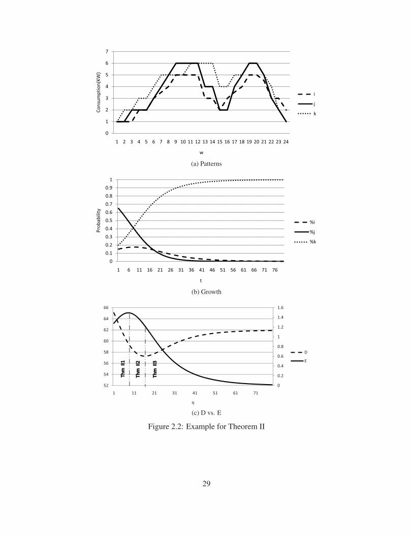
Fig. 2.2b shows the probability changes and Fig. 2.2c presents the behavior of

components and simulates entropy and dis-uniformity of the system for 32 seasons. Fig.

2.2c shows the three different possible areas for Theorem II.

Lemma III: Given two different patterns of behavior (i and j) in the population,

i� j, and given period q= q0:

III.1) Pq0i < Pq0

j and bi > b j i f f Eq0+1 > Eq0 and Dq0+1 < Dq0 i.e. E is increasing in

period (E ↑) and D decreases in period (D ↓) until D = 0 (Xi∫(Ci(w)−Ci)dw =

Xj∫(Cj(w)−Cj)dw) afterward D increases in period (D ↑);

III.2) Pq0i > Pq0

j and bi > b j i f f Eq0+1 < Eq0 and Dq0+1 < Dq0 i.e. E is decreasing in

period (E ↓) and D decreases in period (D ↓) until D = 0 (Xi∫(Ci(w)−Ci)dw =

Xj∫(Cj(w)−Cj)dw) afterward D increases in period (D ↑);

III.3) Pq0i < Pq0

j and bi < b j i f f Eq0+1 < Eq0 and Dq0+1 > Dq0 i.e. E is decreasing in

period (E ↓) and D increases in period (D ↑);

III.4) Pq0i >Pq0

j and bi< b j i f f Eq0+1 >Eq0 andDq0+1 >Dq0 i.e. E is increasing in period

(E ↑) and D increases in period (D ↑).

Proof: To prove this lemma we should consider different sgn(Ci(w)−Ci) between

dis-uniformity of i and j, for all w. So, the total dis-uniformity decreases until 0 and in-

creases after that (because of power of 2 in (2.14)). D= 0 when the weighted dis-uniformity

for all components i is equal to weighted dis-uniformity for all components j. When the

total dis-uniformity increases (Lemma III.3 and III.4) we do not need to consider any min-

imum point, because the function is non decreasing. �

30

Corollary III: When conditions of Lemma III hold and t → ∞:

III.1) In exponential growth ∃ε > 0 where, D< ε (ε is a lower bound for D) and E ∈ (0,1)when D decreases (Lemma III.1 and III.2). Also, Dj is an upper bound for D and

E ∈ (0,1) when D increases (Lemma III.3 and III.4);

III.2) In logistic growth max{0, f (Li)} is a lower bound for D and E ∈ (0,g(Li)) when D

decreases (Lemma III.1 and III.2). Also, min{Dj, f ′(Lj)} is an upper bound for D

and E ∈ (0,g′(Lj)) when D increase (Lemma III.3 and III.4).

Proof: Proof is similar to Corollary I, however for a specificw=w0 where, Xi∫(Ci(w0)−

Ci)dw0 ≈ Xj∫(Cj(w0)−Cj)dw0, we have D ≈ 0. This point may happen before all com-

ponents become similar to i’s so min(D) = 0 where, E �= 0 and E = 0 where, D �= 0. �

Theorem III: Given n different patterns of behavior (i = 1, ...,n) in population S,

bk ≥ 0, ∀k ∈ S and i� j for i ∈ S′ and j ∈ S−S′:

III.1) E <− log2Pi (∑i∈S Pi log2Pi> log2Pi) and bi> b j for i∈ S′ and j∈ S−S′ i f f E is in-

creasing in period (E ↑) and D decreases in period (D ↓) until D= 0 (∑Xi∫(Ci(w)−

Ci)dw= ∑Xj∫(Cj(w)−Cj)dw) afterward D increases in period (D ↑);

III.2) E >− log2Pi (∑i∈S Pi log2Pi< log2Pi) and bi> b j for i∈ S′ and j ∈ S−S i f f E is de-

creasing in period (E ↓) and D decreases in period (D ↓) until D= 0 (∑Xi∫(Ci(w)−

Ci)dw= ∑Xj∫(Cj(w)−Cj)dw) afterward D increases in period (D ↑);

III.3) E <− log2Pi (∑i∈S Pi log2Pi > log2Pi) and bi < b j for i ∈ S′ and j ∈ S−S′ i f f E is

decreasing in period (E ↓) and D increases in period (D ↑);

31

III.4) E >− log2Pi (∑i∈S Pi log2Pi < log2Pi) and bi < b j for i ∈ S′ and j ∈ S−S′ i f f E is

increasing in period (E ↑) and D increases in period (D ↑).

Corollary IV: When conditions of Theorem III hold and t → ∞:

IV.1) Corollary III.1 can be generalized to n components in Theorem III with E ∈ (0, log2 n);

IV.2) Corollary III.2 can be generalized to n components in Theorem III with different f ,

f ′, g, and g′ functions.

Lemma IV: Given two different patterns of behavior (i and j) in the population,

i � j, and given period q = q0; Lemma III.1, III.2, III.3, and III.4 and Corollary III.1 and

III.2 are valid.

Theorem IV: Given n different patterns of behavior (i = 1, ...,n) in population S,

bk ≥ 0, ∀k ∈ S and i� j, for i ∈ S′ and j ∈ S−S′; Theorem III.1, III.2, III.3, and III.4 and

Corollary IV.1 and IV.2 apply.

Example 2: Assume we modify Example 1 to three components with negative dom-

inance, (Fig. 2.3a, Di = 42.99, Dj = 77.33, and Dk = 59.96).

Fig. 2.3b shows the behavior of the complex system and Fig. 2.3c shows the

different possible cases of Theorem IV.

Summary: We summarize the results of Theorem I, II, III, and IV in Table 2.1 and

conclude Theorem V as a general theorem to control decomposability and indicate results

of interactions between components of a complex system in all dominance cases.

32

0

1

2

3

4

5

6

7

1 2 3 4 5 6 7 8 9 10 11 12 13 14 15 16 17 18 19 20 21 22 23 24

Cons

umpt

ion(

KW)

w

i

j

k

(a) Patterns

0

0.1

0.2

0.3

0.4

0.5

0.6

0.7

0.8

0.9

1

1 6 11 16 21 26 31 36 41 46 51 56 61 66 71 76

Prob

abili

ty

t

%i

%j

%k

(b) Growth

1.2

1.4

1.6

50

60

70

0.4

0.6

0.8

1

1.2

1.4

20

30

40

50

60

D

E

0

0.2

0.4

0.6

0

10

20

1 11 21 31 41 51 61 71

E

00

1 11 21 31 41 51 61 71

q

(c) D vs. E

Figure 2.3: Example for Theorem IV

33

Table 2.1: Summary of emergence

− log2Pi > E − log2Pi < Ebi > b j bi < b j bi > b j bi < b j

i� j E ↑ ∧ D ↓ E ↓ ∧ D ↑ E ↓ ∧ D ↓ E ↑ ∧ D ↑i� j E ↑ ∧ D ↓ E ↓ ∧ D ↑ E ↓ ∧ D ↓ E ↑ ∧ D ↑i� j E ↑ ∧ D ↓ (1), D ↑ (2) E ↓ ∧ D ↑ E ↓ ∧ D ↓ (1), D ↑ (2) E ↑ ∧ D ↑i� j E ↑ ∧ D ↓ (1), D ↑ (2) E ↓ ∧ D ↑ E ↓ ∧ D ↓ (1), D ↑ (2) E ↑ ∧ D ↑

(1) if ∑Xi∫(Ci(w)−Ci)dw> ∑Xj

∫(Cj(w)−Cj)dw,

(2) if ∑Xi∫(Ci(w)−Ci)dw< ∑Xj

∫(Cj(w)−Cj)dw.

Theorem V (mechanisms of components): If i� j, i.e., i’s dominate j’s, dis-uniformity

of the system is decreasing in period if the entropy increases in period when − log2Pi > E

or if the entropy decreases in period when − log2Pi < E while, ∑Xi∫(Ci(w)−Ci)dw <

∑Xj∫(Cj(w)−Cj)dw for both conditions.

We can apply this theorem to control or at least predict the complex behaviors in

large ECASs. Here, we provide incentives to motivate the components to decrease the

dis-uniformity by adjusting their patterns (this adjustment changes the growth rates bi’s

dynamically). This heterarchical rearrangement with external changes to the environment

but without central organization is a source of self-organizing in components. As an illus-

tration, assume n patterns of consumption in a system. When n is large (e.g. patterns of

consumers in large metropolitan area), it is impossible to control and predict all behaviors

and their relationships. We can focus on a few groups (pattern i where − log2Pi > E) and

increase the entropy by motivating other consumers to adjust to this pattern (migrate to

this pattern or increase its growth portion). This phenomena makes non-linear complex

dynamic growth rates i.e. bi = K(R(D);E). Here, K is a function of R(D) and population

of other patterns (i.e. E). R(D) shows the motivations based on D (e.g. rewards that con-

sumers receive by cooperating to reduce the dis-uniformity). These changes in bi’s make

Xi dependent on each other. To predict the behaviors at each period, we can map the system

34

conditions (dominance, entropy, and growth rates) to an appropriate theorem. In the next

section we will show how we can control the interoperability between patterns by using a

third pattern (catalyst) i.e. indirectly utilize Theorem V to decrease the dis-uniformity.

2.3 Emergence as the Effect of Interoperability

In Step 2 of the framework (Fig. 2.1), we study the engineering concept of emergence in

ECASs. Bar Yam [85] conceptually and mathematically shows the possibility of defining a

notion of emergence and described four concepts of emergence. Conceptual classification

for emergence is proposed by Halley and Winkler [86]. Prokopenko et al. [73] interpret

concepts of emergence and self-organization by information theory and compare them in

CASs. We borrow concepts from information theory to analyze and predict emergence

behaviors of ECASs and show the applicability of Theorem V.

Consider Xi to be an integer variable that describes the number of components that

follow pattern i in a population with total Q components. Assume there are certain defined

states for proportion XiQ (e.g. low, medium, and high proportion). Let mi,mi = 1, ...,Mi,

present number of defined states for pattern i. We define Pmimj to be the joint probability to

find simultaneously pattern i and pattern j in state mi and mj. These probabilities can be

found by statistical analysis of historical information about the population. For example in

Table 2.2a we consider pattern i has low state when it is 0%-20% and pattern j has medium

state when it is 0%-15% out of the population. Here, Pmimj = P(mi= low,mj =medium) =

0.05 shows the joint probability of 0 ≤ XiQ < 0.2 and 0 ≤ Xj

Q < 0.15 is equal to 0.05 (see

Example 2 for more details).

35

Emergence cannot be defined by properties and relationships of the lower compo-

nent level [81]. Assume there is an interaction between pattern i and j. Then Eq. 2.6

becomes,

E(i, j) =−Mi

∑mi=1

M j

∑mj=1

Pmimj log2Pmimj , (2.16)

We measure the interoperability between i and j which is the amount of information

that i and j share and reduce the uncertainty of each other by

I p(i; j) =Mi

∑mi=1

M j

∑mj=1

Pmimj log2

Pmimj

PmiPmj

, (2.17)

where, Pmi is the marginal probability for State mi. This equation is interaction information

(mutual information) of i and j in information theory. There can be other interoperabilities

in a system such as interoperability between class of agents (Ic, to be formally defined later

in Section 3.2) so, I generally shows the interoperabilities between properties of agents.

We can obtain [84],

E = E(i, j) = E(i)+E( j)− I p(i; j), (2.18)

where, E(i) = I p(i; i) is the self-information of i.

From Eq. 2.18 when I p(i; j) increases (I p ↑), E decreases (E ↓). For the case of

only two groups of patterns in the system, the mutual information is a positive number with

maximum of one, 0 ≤ I p≤ 1 (from Eq. 2.17). E is minimal when i and j are identical, I p=

1 (one group follows the other one) and E is at its maximum when i and j are independent,

I p = 0 (groups are completely autonomic). We can use this property to control the entropy

in Lemma I, II, III, and IV.

The generalization of Eq. 2.18 to three pattern cases is

E = E(i, j,k) =−[E(i)+E( j)+E(k)]− I p(i; j;k)+E(i, j)+E(i,k)+E(k, j), (2.19)

36

where, interoperability I p, can be negative. Let I p(i; j|k) define conditional interoperability

between i and j conditioned on k,

I p(i; j|k) =Mi

∑mi=1

M j

∑mj=1

Mk

∑mk=1

Pmimjmk log2

PmkPmimjmk

PmimkPmjmk. (2.20)

Here, we define Pi jk to be the joint probability to find simultaneously patterns i, j and k in

the State mi, mj and mk, respectively. Then, we obtain,

I p(i; j;k) = I p(i; j)− I p(i; j|k). (2.21)

Positive I p means k supports and increases the interoperability between i and j.

However, negative I p shows k inhibits and decreases the interoperability.

Definition II:

• Catalyst: Pattern k is a positive catalyst for other patterns in the system if k supports

their interoperability and is a negative catalyst if inhibits their interoperability.

Let I p = I(μ),μ = {in0|n0 = 1, ...,n} represents interoperability between patterns

in a system where, in0shows its pattern types that each of them can be appear in mi states.

We can generalize Eq. 2.19 and Eq. 2.21 to n patterns [83, 87],

E(μ) = ∑ν⊆μ,ν �=μ

(−1)(|μ|−|ν |−1)E(ν)− I(μ),

μ = {in0|n0 = 1, ...,n}.

(2.22)

I p(i1; ...; in) = I p(i1; ...; in−1)− I p(i1; ...; in−1|in). (2.23)

Generally for multiple catalyst (k number of catalyst),

I p(i1; ...; in) = I p(i1; ...; in−k)− I p(i1; ...; in−k|i(n−k+1); ...; in). (2.24)

37

In Theorem V instead of increasing or decreasing the entropy we can change the

interoperability. We add catalyst(s) to control (inhibit or support) the interoperability. We

define I p(μ|k) as the conditional interoperability of System μ conditioned on existing new

pattern k.

Definition III:

• Catalyst-Associate Interoperability (CAI): Consider set of patterns that have inter-

operability I p(μ). Then we show the interoperability between patterns when a new

pattern k exists in System μ by I p(μ|k),

CAI = I p(μ|k)− I p(μ). (2.25)

• Effect of Catalyst (EOC): Consider set of patterns that give entropy E(μ) then en-

tropy of the system conditioned on existing new pattern k is E(μ|k),

EOC =E(μ|k)−E(μ)

CAI, (2.26)

where, E(μ|k) and E(μ) are entropy in period q after and before applying the cata-

lyst(s), respectively.

Example 3: (Interoperability in Fig. 2.1) Define the state of population of pattern

i to be low if 0 ≤ Pi < 0.2, medium if 0.2 ≤ Pi < 0.4, and high if Pi ≥ 0.2. Also the state

of population of pattern j is low if 0 ≤ Pj < 0.1, medium if 0.1 ≤ Pj < 0.15, and high if

Pj ≥ 0.15. Assume Table 2.2a is the joint probabilities for states of i and j in Example 1

where population of other patterns and their effects are negligible.

38

Table 2.2: Prior and Posterior joint probabilities

(a) Prior Probabilities for k ≈ 0

P(mi,mj) low medium high

low 0.20 0.05 0.02

medium 0.15 0.15 0.15

high 0.05 0.05 0.18

(b) Posterior Probabilities for k > 0

P(mi,mj|k) low medium high

low 0.23 0.03 0.02

medium 0.15 0.19 0.13

high 0.02 0.03 0.20

From Equations 2.16, 2.17, and 2.18:

E(i) = 1.56, E( j) = 1.54, E(i, j) = 2.90, I p(i; j) = 0.20.

If adding Catalyst k, updates Table 2.2a to Table 2.2b (users k affect the interrelationships

between i’s and j’s),

E(i) = 1.56, E( j) = 1.53, E(i, j) = 2.73, I p(i; j) = 0.36.

So we increase the entropy by increasing the interoperability which decreases the

dis-uniformity in Example 1.

CAI = 0.36−0.2= 0.16,

EOC = 2.73−2.900.16 =−1.06.

We can use the concept of EOC to select an appropriate catalyst. For example

assume n patterns of consumption in a social population where, i1 and i2 have the majority

of population and thus the largest effect on the dis-uniformity of the consumption. We

are planning to decrease the dis-uniformity with a limited amount of resources (e.g. some

rewards to give to cooperative consumers). Instead of distributing the reward between a

large group (say i1) to cooperate with the other group which is not so effective (because the

portion of each individual is too low), we can reward a small group of catalyst (say i3) to

improve the interoperability between i1 and i2. This idea is similar to finding and investing

39

on hubs in a social network (based on power-law the numbers of components with higher

relationships decrease exponentially [34]). The next step is to show how this emergence

phenomena causes evolution in the system.

2.4 Evolution Because of Updates in the Traits

Here (Step 3 of the framework, Fig. 2.1), we analyze the evolution process. Then, in the

last step of the framework (Step 4) we depict the adaptation and learning in the system.

Some measures are developed for the complexity threshold parameter of physical complex

systems in previous studies[88]. Erdos and Renyi[89] study probability threshold function

and evolution in random graphs. We borrow the concept of threshold [89].

Let Mqλ ;λ = 1, ...,λ0 be the number of components which have the trait λ at period

q (such as willingness to adjust consumption pattern for a specific cost saving). The prob-

ability that a system possesses trait λ at period q isMq

λQ . Here, φqλ is a binary variable that

shows the system possesses Attribute λ at period q.

φqλ =

⎧⎪⎨⎪⎩

1, ifMq

λQ ≥ τλ ,

0, ifMq

λQ < τλ ,

(2.27)

where, τλ is the threshold for trait λ .

Let Φq = (φqλ ;λ = 1, ...,λ0) be a vector of 0 and 1’s for λ0 traits where, its λ th

position is 1 if φqλ = 1. Let Ψq be a finite set of Φ’s at period q. Based on the definition, the

system evolves when ∃q> q0,Φq ∈ Ψ(or Φq /∈ Ψ) & Φq0 /∈ Ψ(or Φq0 ∈ Ψ). Where, Ψq is

a predefined finite set of Φ’s at period q.

Definition IV:

• Stagnation: systems are stagnant when they are not evolvable i.e., Φq ∈ Ψ(or Φq /∈Ψ)∀q.

40

Example 3: (Traits in Fig. 2.1) Assume three traits i, j, and k with τi= 0.2, τ j = 0.4,

τk = 0.3, and Ψ= {[0 1 1], [1 1 1]} in Example 1:

q= 4 :Mqi

Qq =26

156 ≤ 0.2

q= 4 :Mqj

Qq =87

156 ≥ 0.4

q= 4 :Mqk

Qq =44

156 ≤ 0.3

⎫⎪⎪⎪⎪⎬⎪⎪⎪⎪⎭

⇒ Φ(4) = [0 1 0],

q= 5 :Mqi

Qq =31

183 ≤ 0.2

q= 5 :Mqj

Qq =95

183 ≥ 0.4

q= 5 :Mqk

Qq =57

183 ≥ 0.3

⎫⎪⎪⎪⎪⎬⎪⎪⎪⎪⎭

⇒ Φ(5) = [0 1 1],

q= 9 :Mqi

Qq =55

367 ≤ 0.2

q= 9 :Mqj

Qq =139367 ≤ 0.4

q= 9 :Mqk

Qq =163367 ≥ 0.3

⎫⎪⎪⎪⎪⎬⎪⎪⎪⎪⎭

⇒ Φ(9) = [0 0 1].

So related to the set Ψ= {[0 1 1], [1 1 1]} the system evolves at q= 5 and q= 9. If

we assume set Ψ contains only [1 1 1] (i.e. the system evolves only when it possesses all

traits) then Φq is never in Ψ and this system is stagnant.

In this example the system is adjusted by two evolutions. This adapting situation

can be non-stationary. In later sections we simulate a case where components adjust their

behaviors several times to increase their objectives. For example, Fig. 2.4a shows the case

that, i, j, and k compete to get more rewards by reducing the dis-uniformity. However,

to reduce the dis-uniformity they should cooperate by adjusting their behaviors (changing

growth rates, bi’s). Adding a learning procedure (do not adjust to previous tried states)

omits the non-stationary evolution and causes faster adaptation in Fig. 2.4b. See Section

4.2 for detailed analyze of this behavior and more information about the simulation.

41

0.9

1

0 7

0.8

0.6

0.7

ess

i

0.4

0.5

Fitn

e i

j

0.2

0.3 k

0

0.1

01 5 9 13 17 21 25 29 33

Time

(a) Non-stationary adaptation

0.9

1

0 7

0.8

0.6

0.7

ess

i

0.4

0.5

Fitn

e i

j

0.2

0.3 k

0

0.1

01 5 9 13 17 21 25 29 33

Time

(b) Fast adaptation

Figure 2.4: A complicated example for adaptation

To extend this framework, the concept of dissection of features can extend to other

ECASs easily. Entropy of components is a general concept for all systems and dis-uniformity

can be interpreted in different ECASs. For example, reducing demand fluctuations in

wholesale marketing, resource allocations in supply chain management, and synergism

of commands to reduce the distances to a target in AI or defense sectors are other types of

dis-uniformity. Decision makers may assign different objectives to ECASs based on their

requirement and they are not limited to dis-uniformity. However, any ECAS of the class

being addressed needs at least one minimizing/maximizing measure to study dissection of

features other than component entropy. Other hallmarks (Evolution and Adaptation) are

driven from the emergence concept (dissection of features and the interactions) and their

mathematical calculation is not limited to electricity usage.

42

Chapter 3

AN AGENT-BASED OPTIMIZATION PLATFORM

We propose a methodology that advances our ability to model and understand engineered

complex adaptive system behaviors through computational intelligence. The development

of this methodology has significant intrinsic merit as it will explore fundamental issues

in multi-layered ECASs and presents new optimization actions and descriptive paradigms.

This ABM presents a novel platform and toolkit that creates a dynamic laboratory to study

properties and behavior of DR in the US Electricity Market as an ECAS. We integrate con-

cepts from social networks (e.g. friendship, scale-free and single-scale networks), social

science (e.g. opinion exchange, media impact, and irrationality), complexity theory (e.g

emergent behavior and adaptation), diffusion theory (e.g. adaptability and innovativeness),

and decision theory (e.g. utility) to build our comprehensive ABM. This model enables

us to integrate optimization rules and build a comprehensive social layer to analyze and

simulate details of social behaviors in ECASs. We justify our model by illustrating its

applicability on the US power system.

In this study, a multi-layer descriptive modeling approach (Fig. 3.1) composed

of conceptual behavior and fundamental entity aspects is considered as the whole system

structure. This approach integrates layers by cross-layer effects, effect of stochastic events

(e.g. system failure and extreme weather condition), and rules of standards and procedures.

Usually, physical layer(s) model networks, their characteristics, and physical components

[90]. In this layer effects of topology and structure of networks have been studied in the

past [49, 50, 51]. Decision/control layer(s) represent different business strategies, opti-

mization models and rules for decision makers (e.g. regulators). Those models are used for

short-term, mid-term, or long-term analysis. Previous modeling approaches such as AMES

[65, 66] are useful for modeling behaviors of this layer. Some models (e.g. EMCAS [67])

43

present a more comprehensive view on different layers. In this study, Social/ Swarm Lay-

ers(s) include the interrelationship between agents and their effects on each other. Also

behavioral properties and attributes of decision makers are considered in this layer (see

Section 3.1/Environment for details and examples of each layer).

Figure 3.1: Integration of the Structural Entity Model

To show cascading of decisions from Decision/Control Layer(s) to Physical Layer(s),

we detail the Social/ Swarm Layer(s). This integration helps us depict emergence in behav-

ioral patterns in the lower level of the system and their effects on evolution in the higher

levels (e.g. predict the result of dynamic pricing and prizes in future). Moreover, we

formulate a consumer-based optimization model and integrate it with the ABM. Then we

include effects of externalities and subjective behaviors in the integrated agent-based op-

timization model. We study the strategies that have critical effects on the decision/control

and social/swarm layers. Useful managerial insights are derived from executing the model.

44

Electricity regulators adjust service attributes (e.g. price and reward functions)

in response to demand fluctuations to motivate the consumer agent to cooperate in bal-

ancing workload. Consumer agents make decisions to maximize their quantitative and

qualitative utilities. They change consumption patterns in response to incentives and to

social education provided by the regulators. Based on the individual and total patterns

of the electricity consumption, agents may receive individual and cooperation rewards.

Moreover, they may have dissatisfaction to change their behavior (Section 3.2/Process

Overview presents details for calculating utilities, rewards, and dissatisfaction). We study

cooperativeness or competition in the consumers game environment by embedding a non-

convex consumer-based optimization model with the agent-based simulation (see Section

3.2/Decision Rules). We study the behavior of consumers under different control and in-

centive strategies. Then, we include intrinsic environment and control factors to the model

dynamics.

Instead of reducing nonlinear systems to a set of causal variables and error terms,

our ABM shows how complex adaptive outcomes flow from simple phenomena and de-

pend on the way that agents are interconnected. Rather than aggregating outcomes to find

a total equilibrium, our ABM presents the evolution of outcomes as the result of the ef-

forts of agents to achieve better fitness. This method allows the study and analysis of the

complexities arising from individual actions and interactions that exist in the real world by

bottom-up iterative design methodologies.

Applying this integrated agent-based optimization model has the following benefits

for the US power system and may lead to a reduction in investment on the power grid

infrastructure:

45

• Motivates consumers to balance the total workload by providing incentives and social

education,

• Encourages agents to cooperate with the grid regulators in high stress times and

environments by communicating energy information,

• Increases the grid’s security and reliability by analyzing its behavior during accidents

or system faults,

• Allows studying complex system response to dynamic pricing and other control

strategies,

• Predicts and controls emergent behavior of the agents and system evolution by math-

ematical modeling in respect to economic incentives and social interactions.

3.1 Agent-based Structure

This section presents an overview of agents’ properties and their environment. We present

more details and mathematical modeling of the framework in Section 3.2. Outcomes of

running the simulation are discussed in Chapter 4.

Decision Makers/Agents

1- Pattern of Consumption: Consider a electricity market system comprised of a large

number consumer agents. We study these agents by a measurable outcome of their behavior

where Cqi (w) presents profile of daily consumption (0 ≤ w ≤ 24 hours) at period q for a

consumer that follows pattern i (formally defined in Section 2.1).

2- Properties of Agents: Agents have the capability to present new behaviors by in-

teraction and dependent to other agents. They can switch to new patterns and change their

attributes based on their current properties and neighborhood relationships. We represent

the influence on an agent from another agent by interoperability (will be defined math-

46

ematically in the next section). We initiate a social network of consumer agents where,

Xi(0) is the initial size of the population for each pattern and the population of each pattern

(Xi; i= 1, ...,n) can grow with growth rate, bi, exponentially. Agents may switch from one

pattern to another based on the attributes of the patterns (namely; price, convenience, and

glamour) or through influences of these in their social network. Price defines the total cost

of consumption in a 24 hour cycle time for the related pattern. Convenience shows how

fast and easy consumers can make a decision to switch to this pattern. Glamour shows the

effects of advertisement or other fashion attributes of the patterns. These micro interrela-

tionships make new networks and update the structure of the population in the macro level

of the system.

2- Influences on Agent Decisions: Fig. 3.2 shows how agents are influenced in the

system. Ovals present uncertain variables. Rectangles show the variables that the agents

have the power to modify or select. Hexagons are measurable outcomes. Arcs denote di-

rect influences. Dashed arcs indicate there are some influences; however, the values can be

calculated from other variables with direct influences. Agents consume electricity based on

the environment conditions (e.g. seasonal weather conditions and time of the day) and con-

sumption attributes (e.g. price of electricity consumption and advertisements). This con-

sumption shapes their pattern of behaviors. The entropy of the system, E = −∑Pi log2Pi,

is defined by the frequency of these patterns and the interrelationships between the agents

(i.e. emergent behavior of agents, interoperabilities, and willingness to effect or follow

each other). This entropy of the patterns in a system, yields the dis-uniformity (Eq. 2.14)

of the whole system. Cooperation reward (Eq. 3.11) can be measured based on the regula-

tor’s decisions. Consumers measure their profit (Eq. 3.10) on the bases of the cooperation

reward, their individual rewards, their dissatisfaction, and qualitative utilities. Individual

rewards (Eq. 3.12) and dissatisfaction (Eq. 3.13) are calculated based on the patterns of

47

individual behavior. Qualitative utilities (Eq. 3.9) are functions of the consumption at-

tributes. This total profit makes the agents change their consumptions in the cooperative

game model to adapt to the new environment.

Environment�conditions�

Consumption�attributes��

Agent�consumptions�

Patterns�of�behaviors�

Entropy�of�the�system�

Dis�uniformity�of�the�system�

Cooperation�Rewards�

Consumer�profit�

Interoperability�between�the�agents�

Regulator’s�decisions� Individual�

Rewards�

Dissatisfaction�

Qualitative�values�

Figure 3.2: Influence Diagram

We can characterize the agents as follows (they will be discussed and defined by

details in the next sections):

• Each agent runs a pattern that has three attributes (price, convenience, and glamour),

• Agents connect to each other based on a complex network,

• An agent has desirability coefficients and importance weights for each attribute,

• Agents belong to interoperability classes based on their node degrees,

48

• An agent (partially or fully) optimizes its profits based on optimization rules in co-

operation with other agents,

Environment/Patches

Figures 3.3, 3.4, and 3.5 present an overview of a three-layer image of our modeling study.

The Decision/Control Layer (Fig. 3.3) includes strategies (e.g. dynamic pricing), optimiz-

ing (e.g. maximum profits and peak reduction), plans (e.g. new generators), investments

(transmission and distribution infrastructure), and information sharing (e.g. communicate

energy information). In the US energy system Independent System Operators (ISOs) and

Regional Transmission Organizations (RTOs) work in this layer of the complex system.

Strategies (e.g. dynamic pricing)

Optimizing (e.g. maximum profits and peak reduction)

Plans (e.g. new generators)

Investments (e.g. transmission and distribution infrastructure)

Information sharing (e.g. communicate energy information)

S i

um ion)

estments (e.g. tratratrtransmnsmnsmnsmiiissiondistribution infrastructure)

(e.g.

profits and peak reductiion)

and

information)

Inveand

Plans (e.g. new generators)

)n )

es (e.g. dynamic pricing)Strategie

Regulator(s)

Figure 3.3: Decision Layer

The Social/ Swarm Layer (Fig. 3.4) considers interrelationships between agents and

preferences. We can consider bounded rationality for agents and externalities (e.g. fashion

49

effects) in this layer. Non-physical attributes of agents (e.g. glamour) and their utility

function can be studied and analyzed here. We will discuss how the behavior of agents as

a group emerges in this layer and converges to a steady pattern. Learning algorithms (e.g.

reinforcement learning) and adaptation scenarios can be considered in this layer.

Bounded rationality Externalities (e.g. fashion effects) Learning algorithms (e.g. reinforcement learning)

Figure 3.4: Social layer

The Physical Layer (Fig. 3.5) includes features, mechanism of components of the

system, and their physical network. In the energy system example this layer includes gen-

erators (e.g. main power plant, wind forms, solar panels, and small generators), distributors

and transmission, and consumers (e.g. homes, businesses, and industries). The topology of

networks is considered in this layer.

The Social /Swarm layer helps us to cascade effects of the Decision/ Control layer(s)

to the Physical layer(s) by modeling the emergence and adaptation of the whole swarm.

50

Components Features Networks

Figure 3.5: Physical Layer

The topology of connectedness and protocols for interaction in the network are important

properties of the network for our study. The topology of interactions defines who is, or

could be, connected to whom. The protocols of interactions are the mechanisms of the dy-

namics of the interactions. Both specify the local information accessible to an agent. The

structure of the network (e.g. scale-free or single-scale properties) helps us to calculate the

class of interoperability for each agent and find its influencer nodes. We assign the class of

an agent based on the size of the network and the degree of the node. Also, we consider

the pattern of behavior for each consumer. The distribution of patterns of behaviors and

the way the agents are seeded with patterns are important. We present the value of inter-

operability between two agents as the weights of the edges. In summary, three parts of the

network are used in our ABM (they are mathematically defined in the next section):

51

1. Patterns of nodes (consumer agents),

2. Degree of agents that is related to the structure of the network,

3. Weights of edges that show the interoperability of agents.

We assume the social network G between agents with preferential attachment and

growth can be represented by a scale-free network [35, 49, 50, 91]. Where |E(G)| shows

the number of links in the social network G. The nodes of the network depict autonomous

consumer agents while the edges symbolize the influences or interoperability between the

agents. The node degree distribution of the network follows a power law i.e., the probability

a node has κ edges is cκ−λ where, c is a normalization constant and λ defines the shape

of the distribution [92, 93]. We will relax this assumption to study single-scale behavior

of a Gaussian network later. The size of the network may grow by period while its scale-

free/single-scale characteristic remains valid.

3.2 Agent-based Optimization Engine

This section presents the detail procedure of decision rules to show how agents optimize

their actions and change their behaviors.

Process Overview and Scheduling

Fig. 3.6 shows the logical flowchart of the agent-based process and its scheduling. The

flowchart includes three main sections: setup, switch, and optimize.

1- Setup section initiates the scale-free network of interrelated consumers and seeds

them with the patterns of consumption. Assume initially that agents are independent (this

assumption will be relaxed later to induce complex behavior). Population of pattern i

(Xi; i = 1, ...,n) changes exponentially with growth rate bi at period q, q = 1, ...,T (Eq.

2.1). For pattern probability Pi = Xi∑Xi then the growth of entropy follows Eq. 2.8. Here, at

52

Increment�the�time�period�

Seed�the�population�with�the�pattern ratios�

Set�the�agent�population�and�the�scale�free�network�

Assign�desirability�coefficients�and�attribute�weights�to each�agent

Update dis�uniformity and�Entropy�of�the�system�

Find�the�interoperability�class�of�agents�based�on�the�network�protocol

Start�

Compute�the�interrelationship�of�agents�based�on interoperabilities��

Switch�to�the�agent�with�first/second�highest�

interrelationship�

Calculate�the�agent�utilities based�on�the�desirabilities�

Compute the�cooperative reward�based�on�the�system�dis�uniformity�and�individual�agent�

rewards�based�each�agent�dis�uniformity�changes�

Calculate�the�agent�dissatisfactions�based�on�difference�of�new�and�switch patterns�

New���>��Old���

N�

Y�

Grow�the�network�based�on�the�fitness�rates�

Calculate�the�value for�the�total reward���

Find�the�agent�with�first/second�highest�interrelationship

SetupSw

itchO

ptimize

Figure 3.6: Logical Flow Chart for Scheduling of the Process Overview

53

each time increment, new agents create ρ connections with previous agents based on the

scale-free property where ρ is a random number between 1 and ρmax. Here ρmax defines the

max link generation. We assign desirability coefficients and attribute weights to the agents

that will be used to compute optimization decisions (to be formally defined later).

We measure the agents’ level of cooperation by the dis-uniformity of aggregated

pattern consumption at period q. The dis-uniformity of pattern i is shown in Eq. 2.13.

The regulators strive to motivate the decision makers (consumer agents) to cooperate and

achieve in such a way that the aggregate consumption in each period is uniform over time.

Thus, we seek to minimize the total dis-uniformity, Eq. 2.14.

The total Dis-uniformity, Eq. 2.14, could be reduced by incentives that change one

or more profiles or rearrange probability of patterns. We will show interactions between

agents and their interoperability effects on dis-uniformity of the system.

2- Switching section defines a set of rules for finding a switching target based on in-

teroperability of agents. We define four sets of classified interoperability for the social layer

population on the basis of the network protocol. This classification shows the agent’s abil-

ity to connect and effect each other where, δυ shows the class of agent υ ,υ = 1, ...,∑ni=1Xi.

Influencers(INF) have the highest number of connection links (interoperability). They

maintain central positions in the social network and their numbers are small. Based on

behavioral profiles, we classify agents by type INF, EF, LF, and ISL. Early Followers(EF)

are more localized and have less interoperability compared to the influencers. Late Follow-

ers(LF) are classified between the Early Followers and Isolated categories. Isolated(ISL)

have low interoperability. They do not have a big influence on other individuals and are

insensitive to others. The idea of this classification is similar to the term innovativeness cat-

egories in diffusion theory by Rogers [94]. However, innovativeness categories consider

speed of adaptation while we consider influences and interoperability in a network.

54

The network node degree distribution follows a scale-free power-law and the node

degrees depend on the network size. To measure the interoperability classification based

on this protocol we need to linearize the power-law functions. We use Eq. 3.1 as the

linearization function and Eq. 3.3 shows how the power-law functions are linearized for

each classification.

Lin(αδυ ,βδυ ) = αδυ .ln(|E(G)|)−βδυ , (3.1)

where,

δυ ∈ {INF,EF,LF, ISO},

αINF > αEF > αLF > αISO,

βINF > βEF > βLF > βISO,

(3.2)

and, |E(G)| shows the number of links in the social network G (total number of interoper-

ability links). Degυ is the degree of agent υ in the network i.e. the number of interoper-

ability connections that each consumer makes in the system.

δυ =

⎧⎪⎪⎪⎪⎪⎪⎪⎨⎪⎪⎪⎪⎪⎪⎪⎩

INF, if Degυ ≥ Lin(αINF ,βINF),

EF, if Lin(αEF ,βEF)≤ Degυ < Lin(αINF ,βINF),

LF, if Lin(αLF ,βLF)≤ Degυ < Lin(αEF ,βEF),

ISL, o.w.

(3.3)

In summary, to classify the agents we chose α and β (see an example in Chapter

4). Then the size of the network and the degree of the node determine the agent classes.

We will use these classes to assign interoperability between agents and calculate their in-

terrelationship.

For agent υ consider all other agents that are connected to υ . The influence on

agent υ from agent z is based partly on the classes of the two agents. Let Icδυ δz represent

interoperability between classes of agents. Here, Icδυ δz is a monotonic function of the in-

fluence that a agent of Class δz has on a agent of Class δυ . Interoperability is a positive

55

number with maximum of one where, Icδυ δz = 0 shows autonomic (independent) class of

agents and Icδυ δz = 1 when they follow each other (identical). Table 3.1 shows an example

of an interoperability classification matrix. Chapter 4 discusses how to measure realistic

values for this table.

Table 3.1: Interoperability between consumer agents

Icδυ δz INF EF LF ISLINF 0.8 0.6 0.4 0.3

EF 0.6 0.5 0.3 0.2

LF 0.4 0.3 0.2 0.1

ISL 0.3 0.2 0.1 0.001

Self-preference θυz, lets agents vary their individual interoperability i.e. it lets two

agents have different interoperability with a specific agent even if all three of them are in the

same set of classification. We assume that the interoperability matrix defines a maximum

possible value for all pairs of classification sets and 0.5 ≤ θυz ≤ 1 may vary this value

to half of its maximum. θυz = 1 shows agent υ does not have any self-preference and

follows the interoperability matrix. Note if θυz = 0, the model will be modified to a system

without the network. To simplify the formulation we use θυδz =∑z∈δz θυzXz∈δz

, average self-

preference, in Eq. 3.4. For example, assume consumer 1 has two neighbors (consumers 2

and 3) and all three of them are INF . Based on Table 3.1, consumer 1 can have maximum

interoperability 0.8 with both neighbors. However she/he may has less willingness to be

affected by consumer 3. Then consumer 1 reduces its interoperability to 0.4 by selecting

self-preference equal to 0.5 (See more examples in Figures 3.7a and 3.7b).

The interrelationship ℜ, between agents will be assigned based on the interoper-

ability, Ic, matrix and their classification. Assume Xδzi is the number of connected agents

(neighbors) to agent υ in class δz with pattern i. To calculate interrelationship of agent υ

with its neighbors in pattern i we used Eq. 3.4,

56

ℜυ i =∑δz θυδz .I

cδυ δz .Xδzi

∑δz ∑i Xδzi, i= 1, ...,n,υ = 1, ...,Q, (3.4)

where, Icδυ δz is the interoperability of the agent in class δυ with agent in class δz where

δz ∈ {INF,EF,LF, ISO}.

To select an appropriate pattern as a switching target, we use Eq. 3.5 or Eq. 3.6

allowing the agent to consider the strongest or top two alternatives held by connected agents

where, switchqυ is the pattern that agent υ chooses as the switching target at period q. The

agents have two ways to select their target. Eq. 3.5 lets an agent compare its objective with

the objective of its highest weighted interrelationship neighbor. Here the switching target

of agent υ is the pattern of an interconnected agent with the highest interrelationship in its

neighborhood. To consider the agent tendency to stay in her current pattern, we add a fixed

amount of the awareness-threshold ϒυ (a user-defined variable) divided by total number

of agents to her interrelationship with her current pattern i.e., ℜυ i =ℜ0υ i+

ϒυTotalNeighbors if

i=Pattern(υ), where ℜ0υ i is her current interrelationship.

switchqυ = argi{max(ℜυ i)}, ∀i. (3.5)

To avoid similar patterns when the agent with the highest interrelationship has the same

pattern with the target, we may use Eq. 3.6 to let agents look at the second highest interre-

lationship.

switchqυ = argi{max(ℜυ i)}, ∀i �= Pattern(υ). (3.6)

Example 1: Fig. 3.7a presents an example for calculating interrelationships. As-

sume consumer υ is an agent trying to decide whether to switch her consumption pattern.

Agent υ is an influencer agent, INF and six other agents are connected to this agent. Two of

57

them follow pattern i (1 EF , 1 LF), three of them follow pattern j (1 INF , 1 EF , 1 LF), and

one of them follows pattern k (INF) at this time. Assume the awareness-threshold ϒυ = 0

and the agent υ does not have any self-preference i.e., θυz = 1. Then ℜυ i =0.6+0.4

6 = 0.17,

ℜυ j =0.6+0.4+0.8

6 = 0.3, and ℜυk =0.86 = 0.13. Hence, if agent υ has the pattern j the

switching target switchqυ = i from Eq. 3.6 and switchqυ = j otherwise.

Example 2: Fig. 3.7b continues Example 1 by adding a self-preference to the agent

υ for one of its neighbors (underlined number in the arc). This means agent υ prefers to

weigh the interoperability of the EF class of pattern i by half (θυ i = 0.5). We calculate

ℜυ i =0.5∗0.6+0.4

6 = 0.12 changing switchqυ = k if we use Eq. 3.6 and Pattern(υ)= j.

v�

i� i�

J

J�J�

K�

INF

LF

LF

INFEF

EF

INF

0.8

0.80.6

0.4

0.40.6

(a) Without self-preference

v�

i� i�

J

J�J�

K�

INF

LF

LF

INFEF

EF

INF

0.8

0.80.6

0.4

0.40.6

0.5

(b) With self-preference

Figure 3.7: Calculating the Interrelationship

3- Optimizing section: once a target pattern is defined, the agent has to decide

whether to keep her current pattern or to switch based on the pattents’ utility functions,

rewards, and dissatisfactions. The total utility value of a pattern is a weighted average

of the desirability score Ωυs that is a number between 0-1 for each attribute [95]. Recall

that the attributes are price, convenience, and glamour. Here, Ωυs shows the desirability

score of agent υ for attribute s. When the agents target the maximum value of an attribute

58

(e.g. glamour), to calculate the desirability, we use Eq. 3.7 where y shows the value of

the attribute and L and U are its lower and upper bound in Fig. 3.8a. We apply Eq. 3.8

when the target is a minimum value, Fig. 3.8b (e.g. time to make decisions or cost of

changing behaviors). The Desirability coefficient γυs, parameterize the desirability score

Ωυs. Desirability functions showing (γ < 0) characterizes risk-averse agents and (γ > 0)

characterizes risk-seeking agents if the agent targets a maximum and vise versa if the agent

targets a minimum.

Ωυs =

⎧⎪⎨⎪⎩

1−exp(γυs∗ ys−LsUs−Ls )1−exp(γυs)

, if γυs �= 0, υ = 1, ...,Q,s= 1,2,3,

ys−LsUs−Ls , if γυs = 0, υ = 1, ...,Q,s= 1,2,3.

(3.7)

Ωυs =

⎧⎪⎨⎪⎩

1−exp(γυs∗Us−ysUs−Ls )1−exp(γυs)

, if γυs �= 0, υ = 1, ...,Q,s= 1,2,3,

Us−ysUs−Ls , if γυs = 0, υ = 1, ...,Q,s= 1,2,3.

(3.8)

Risk�seeking�

Risk�averse�

Risk�Neutral�

yUL�

1�

��

� < 0

� = 0

� > 0

(a) targeting maximum

Risk�seeking�

Risk�averse�

Risk�Neutral�

1�

L� Uy

��

� > 0

� = 0

� < 0

(b) targeting minimum

Figure 3.8: Desirability Functions

The Utility ValueUυ , is the weighted average of the desirability scores of its pattern

attributes. Agents can assign their own importance weight Wυs, to different attributes to

have individual value functions (Eq. 3.9).

59

Uυ =∑sWυsΩυs

∑sWυs, υ = 1, ...,Q,s= 1,2,3. (3.9)

Agents receive two types of rewards when they switch to new patterns. The Co-

operation reward R̂, is a function of the total dis-uniformity. An agent may receive this

reward without any switching when their current pattern cooperates with others to reduce

the dis-uniformity i.e. cooperation reward will be payed to all agents based on the total dis-

uniformity that they create. The Individual reward Rυ , reflects the controllers individual

rewards to the agent based on the contribution of the agent pattern to the central objec-

tives. Agent will receive more individual reward when they choose to change their pattern

of behavior in the way that minimizes their dis-uniformity. Dissatisfaction ϕ , is the only

variable that has a negative effect on the decisions. Dissatisfaction will be measured based

on the amount of difference between new and old pattern of each agent. We assume the

more each agent changes its pattern the more dissatisfaction with its decision (see Section

3.2 for the formulations).

At the end of each period the pattern of the agents are updated as follows:

1. In a growing network, the new network expanded from the old one,

2. Agent classes are redefined based on the network topology,

3. Interoperabilities are reassigned to the network (weight of edges),

4. Self-preference of agents are added to the edges,

5. Interrelationships between agents are recalculated,

6. A target pattern will be selected based on the chosen switching rule,

7. The agent applies a decision rule based on value of perceived choices.

60

Decision Rules

In the previous section we described how an agent determines the utility value of a possible

switching target. A consumer-based optimization will be executed in order to determine

if switching actually occurs. Decision makers (consumer agents) desire to maximize their

total reward πυ . The total reward is a normalized sum of the cooperation reward R̂, the in-

dividual reward Rυ , the utility valueUυ , and dissatisfaction ϕ of the agents. The consumer-

based optimization compares the anticipated total reward πq+1υ (Cqυ(w),C

qswitch(w)) with the

reward obtained continuing the current pattern, πq+1υ (Cqυ(w),C

qυ(w)). If

πq+1υ (Cqυ (w),C

qswitch(w))

πq+1υ (Cqυ (w),C

qυ (w))

>

switching threshold ϒ′υ , the agent switches her pattern to the pattern given by the possible

switch in the period q+1. A general model for agent υ at period q would be,

πqυ = kr̂R̂q+ krRqυ + kuU

qυ − kϕϕq, (3.10)

where,Uqυ is defined by Eq 3.9 and

R̂q = f0(Dq), ∀q, (3.11)

Rqυ = f ′0(Dqυ), ∀υ ,q, (3.12)

ϕqυ = f2(C

qυ(w),C

qswitch(w)), ∀υ ,q,w. (3.13)

The maximization is to be taken relative to the decision that agent υ can make in period

q. To be specific, we choose the cooperation reward R̂q a decreasing exponential function

of the total dis-uniformity (defined in Eq. 2.14) at period q, f0(Dq) = λ0eDqλ00 , and the

individual rewards Rqυ a decreasing exponential function of the individual dis-uniformity

(Eq. 2.13) of each agent at period q, f ′0(Dqυ) = λ ′

0eDqυ λ ′

00 . Values of λ0, λ00, λ ′0, and λ ′

00

are constants and will be assigned later in this study. We choose the dissatisfaction ϕqυ

to be a logarithmic function of the differences between current and previous pattern of

consumption behavior, f2(Cqυ(w),C

qswitch(w)) =

ln(∫ w0

0 |Cqυ (w)−Cqswitch(w)|dw)λ2

. The value of λ2

61

will be assigned later in this study (see Chapter 4 for an example about the functions).

Note that this presents the agents decision model. Above this sits the master problem

of the controlling entity who sets prices and rewards in order to induce desired behavior

(consumption).

Termination Rules

The simulation continues the flow described in Fig. 3.6 until one of the following termina-

tion rules apply:

• The patterns do not change any more,

• A maximal period (simulation time) has been reached.

62

Chapter 4

SIMULATION OF ELECTRICITY MARKETS AND ANALYZING BEHAVIORS

Here is an example to show how our integrated Agent-based optimization model simu-

lates and analyzes the emergent behavior of consumption patterns. This study enables the

electricity regulators to examine the effect of social interactions topologies with more real-

istic cognitive behaviors and improves the efficiency and effectiveness of demand response

and peak reduction programs via behavioral-based incentives (e.g. social education and

advertisement).

4.1 Specifying the Parameters

To illustrate the dynamic behavior of our system we assume three patterns of consumption.

Fig. 4.1 shows the behavior of those patterns in 24 hours (see [96, 97] for more patterns).

0

1

2

3

4

5

6

7

1 2 3 4 5 6 7 8 9 10 11 12 13 14 15 16 17 18 19 20 21 22 23 24

Cons

umpt

ion(

KW)

w

i

j

k

Figure 4.1: Patterns of Consumption

Table 4.1 presents the variables for running the agent-based simulation model. We

assume convenience of a pattern is a qualitative variable between 2 to 5. Lower values

indicate more convenience (it is a scale of the time that agents should spend to feel conve-

63

nient). Glamour is a qualitative variable with higher values implying more fashionable or

advertised patterns.

Table 4.1: State Variables for Running the Simulation

Parameter Variable Range Units Default Area*Initial Population υ = 1, ...,∑i Xi 100- inf # of consumers 500 E

Initial Patterns Xi∑i Xi

, i= 1,2,3 0 to 1 % of total population 0.15,0.65,0.20 E

Growth Rate bi, i=1,2,3 0 to 1 % of pattern population 0, 0, 0 EMax Link Generation ρmax 1 to 10 number 1 EPrice S1 3-8 Currency (cents/KWh) 5, 5, 5 CConvenience S2 2-5 Qualitative 4, 4, 4 CGlamour S3 1-10 Qualitative 3, 3, 3 CDesirability Coefficient γυs ∼Normal (0, 4) N/A N/A AAttribute Weight Wυ ∼Normal (1, 0.2) N/A N/A AAverage Self-preference θυδz ∼Uniform (0.5, 1) N/A N/A A

* Here E, C, and A stand for Environment, Consumption and Agents respectively.

Consumers are autonomous and receive γυ , Wυ , and θυδz identically from sam-

pling random Normal and Uniform distributions ignoring negative samples. To classify

the consumer agents based on their interrelationships, we assume αINF = 4.5, αEF = 2.5,

αLF = 1.5, βINF = 17, βEF = 9, and βLF = 5. These assumptions are created by fitting

a linear function to the growth of degree of the nodes in the network. Fig. 4.2 shows

how these assumptions are used to make linear growth for the degree of nodes at each

class of interoperability. Moreover, we assume f0(Dq) = 100eD(t)10 , f ′0(D

qυ) = 100e

Dυ (t)10 ,

and f2(Cqυ(w),C

q−1υ (w)) = ln(

∫ w00 |Cqυ (w)−Cqswitch(w)|dw)

2 . These parameters are defined to pro-

vide proper scaling and their impetus is discussed in previous sections.

To define interoperability between agents we use the results of empirical studies

on spread of happiness [98], dynamics of smoking [99], and formal/informal influence in

adoption [100]. Fowler and Christakis [98] and Christakis and Fowler [99] classify indi-

viduals in large social networks based on their influence and study probability of changing

behaviors (smoking habits and happiness) in agents when their connected agents adopt to a

new behavior. Based on both studies we conclude that the probability to influence a partic-

ipant in the same class is approximately 50%, 35%, 25%, and 10% for the classes of close

64

20

30

40

50

60

Deg

ree�

of�a

gent

sINF

EF

0

10

1 11 21 31 41 51 61 71 81 91

D

Period

LF

Figure 4.2: Linearized Growth Functions

friend, friend, spouse, and colleague receptively. Tucker [100] showed that authority struc-

ture like the one between managers and workers will add to or subtract to the influences

determined in the previous studies. Based on these studies we choose the interoperability

between the two classes of agents as shown in Table 4.2. These interoperabilities are se-

lected for consistency with the finding of the three mentioned comprehensive studies but

are not uniquely determined.

Table 4.2: Measuring the Interoperabilities

Icδυ δz INF EF LF ISLINF 0.79 0.4 0.1 0.002

EF 0.65 0.51 0.25 0.03

LF 0.41 0.35 0.29 0.06

ISL 0.28 0.2 0.15 0.1

4.2 Analyzing Behaviors

We study the behavior of the integrated agent-based optimization system under a variety

of different circumstances. We examine how the agents’ tendency to stay on their own

pattern (awareness-threshold) effect the distribution of entropy of the system. We define a

baseline awareness-threshold based on previous studies. Then we show how the regulators

65

can improve the effect of a social network. Also we build more realistic results by consid-

ering limited rationality in cognitive capabilities of agents. Finally, we show the effect of

saturated friendship behavior in the system.

The Effect of The Awareness-Threshold

To study behavior of the system we run the model with the default values in Table 4.1

while we modify the awareness-threshold ϒ from 0.00 to 0.32 in 0.02 increments (for

larger thresholds the system will not converge in 400 time periods). Fig. 4.3 shows the

results of 300 runs. This figure shows the distribution of the time to converge as a function

of awareness-threshold ϒ. This time is defined as the time when the entropy of the system

is less than 0.3364 i.e. when at least 95% of agents converge to a pattern (here is Pattern i).

200

250

300

350

400

450

Tim

e�Pe

riod

Min

10%

1st�Qua

Median

3rd Qua

0

50

100

1500 0.02

0.04

0.06

0.08

0.1

0.12

0.14

0.16

0.18

0.2

0.22

0.24

0.26

0.28

0.3

0.32

Awareness�Threshold

3rd�Qua

90%

Max

Figure 4.3: Convergence of the Entropy

Fig. 4.4 depicts a vertical slice from Fig. 4.3. We see how the distribution of

convergence to pattern i shifts from left to right by increasing the awareness-threshold ϒ.

The convergence time increases by increasing the awareness-threshold i.e. the agents have

66

more tendency to stay in their current pattern and converge slower. Fig. 4.5 compares

the average entropy of systems with different awareness-thresholds. Larger awareness-

thresholds cause higher entropy in the system because the system converges slower and

has more agent diversity by period. For very large awareness-thresholds (e.g. 0.3), the

system does not converge in 400 periods. At the beginning of the simulation, the entropy

may increase because the agents may start to switch from a high populated pattern to a low

populated one.

16

12

14

16

ence

8

10

12

Conv

erge

6

8

uenc

y�of

�C

2

4

Freq

u

0

1 17 33 49 65 81 97 113

129

145

161

177

193

209

225

241

257

273

289

305

321

337

353

369

385

Ti P i dTime�Period

(a) Awareness-Threshold=0

9

7

8

9

ence

5

6

Conv

erge

3

4ue

ncy�

of�C

1

2

Freq

u

0

1 17 33 49 65 81 97 113

129

145

161

177

193

209

225

241

257

273

289

305

321

337

353

369

385

Ti P i dTime�Period

(b) Awareness-Threshold=0.1

8

6

7

8

ence

4

5

6

Conv

erge

3

4

uenc

y�of

�C

1

2

Freq

u

0

1 17 33 49 65 81 97 113

129

145

161

177

193

209

225

241

257

273

289

305

321

337

353

369

385

Ti P i dTime�Period

(c) Awareness-Threshold=0.2

6

5

6

ence

3

4

Conv

erge

2

3

uenc

y�of

�C

1Freq

u

0

1 17 33 49 65 81 97 113

129

145

161

177

193

209

225

241

257

273

289

305

321

337

353

369

385

Ti P i dTime�Period

(d) Awareness-Threshold=0.3

Figure 4.4: Distribution of Convergence to Pattern i

Establishing a BaseLine

It has been observed that only 5% of end users are currently empowered to react to the real-

time or day-ahead locational marginal price (LMP) and participate in DR Programs [17].

In order to calibrate our agent-based simulations, we will determine a awareness-threshold

that generates a change in pattern over time that is as close as possible to an simulation

67

502058 1.387334 1.306998526618 1.433907 1.332431521885 1.463869 1.354272

05751 1.485003 1.372586486321 1.50028 1.3886721.2

1.4

1.6

1.8

y486321 1.50028 1.388672467249 1.510736 1.402339

44456 1.517728 1.415224420105 1.521325 1.426525

39821 1.522141 1.43672474004 1.52085 1.44622134836 1.518426 1.45440722206 1 515625 1 46199

0

0.2

0.4

0.6

0.8

1

1.2

1.4

1 21 41 61 81 01 21 41 61 81 01 21 41 61 81 01 21 41 61 81 01

Entr

opy

Th=0

Th=0.1

Th=0.2

Th=0.30.3364

22206 1.515625 1.46199298723 1.511883 1.468582274652 1 506561 1 474632

0

0.2

1 21 41 61 81 101

121

141

161

181

201

221

241

261

281

301

321

341

361

381

401

Time�Period

Figure 4.5: Convergence of the Average Entropies

without a network and 5% participation rate. We quantify the closeness of two simulations

by registering the average percentage of population P(1)iq and P(2)iq of pattern i in the system

as function of time period q. The difference H (Eq. 4.1) is the absolute sum of difference

pattern over time:

H =∑i

∑q|P(1)iq −P(2)iq | i= 1,2,3; q= 1, ...,400. (4.1)

Fig. 4.6 shows the total difference H between an agent-based simulation without

network (5% participation) and an agent-based simulation with a social network as a func-

tion of the awareness-thresholds.

Based on Fig. 4.6 awareness-threshold between 0.08 to 014 yields the most simi-

lar behavior with current systems without networks. For example Fig. 4.7 compares the

emergence in the pattern of behavior in the first ten runs for awareness-threshold=0.1 and

0.3.

68

0.4

0.5

0.6

0.7

0.8

0.9

Tota

l�diff

eren

ce�H Min

10%

1st�Qua

Median

3 d Q

0

0.1

0.2

0.3

0 0.02

0.04

0.06

0.08

0.1

0.12

0.14

0.16

0.18

0.2

0.22

0.24

0.26

0.28

0.3

0.32

T

Awareness�Threshold

3rd�Qua

90%

Max

Figure 4.6: Total Difference With and Without a Social Network

Improving Effect of the Network

We can assume a well designed social network can increase the number of friendships

and/or decrease awareness-threshold of agents (i.e. decrease the tendency to stay in their

initial behavior). Here we show the behavior of the system when we increase max link

generation ρmax. Fig. 4.8 compares the results of networks with ρmax = 1 and ρmax = 3

(i.e. average link generation equal to 2) when awareness-threshold is equal to 0.1. This

figure shows how the social network increases the effects of economical incentives.

We checked the behavior of the topology of the network by log-log plots [34, 101].

Fig. 4.9 compares the scale-free behavior of the network for ρmax = 1 and ρmax = 3 and

depicts the scale-free metric λ increases from 1.47 to 1.81 when we increased ρmax. This

shows how regulators can improve the convergence time by sharing information between

agents or by encouraging them to increase their friendships via social electricity networks.

69

1.2

1

0.8

Popu

lati

on

0 4

0.6ce

ntag

e�of

�P

0.2

0.4

Perc

0

1 13 25 37 49 61 73 85 97 109

121

133

145

157

169

181

193

205

217

229

241

253

265

277

289

301

313

325

337

349

361

373

385

397

1 1 1 1 1 1 1 1 2 2 2 2 2 2 2 2 3 3 3 3 3 3 3 3 3

Time�Period

(a) Awareness-Threshold=0.1

1 2

1

1.2

tion

0 6

0.8

f�Pop

ulat

0.4

0.6

enta

ge�o

f

0.2Perc

e

0

1 17 33 49 65 81 97 113

129

145

161

177

193

209

225

241

257

273

289

305

321

337

353

369

385

401

Ti P i dTime�Period

(b) Awareness-Threshold=0.3

Figure 4.7: Comparison of Awareness-Threshold=0.1 and 0.3

Externalities and Irrationality

Some characteristics of agents (such as irrationality) and the effects of externalities (such

as a fashion effect) are not considered in most of the previous studies on ABM of electrical

CASs. We analyze the impact of these factors on the social/swarm layer by incorporating

them into the agent decisions and study their effect on objectives and control strategies.

Considering irrationality helps us to create more realistic cases. We propose discrete choice

models (Eq. 4.2) based on the total reward π and the interoperability classification to study

70

400

450

300

350od

200

250

Tim

e�Pe

rio

Th=0.1,��_max=1

Th=0.1,��_max=3

100

150

T

0

50

Min 10% 1st Qua Median 3rd Qua 90% MaxMin 10% 1st�Qua Median 3rd�Qua 90% Max

(a) Convergence of the Entropy

6

8

10

12

14

16

18

ency

�of�C

onve

rgen

ce

Th=0.1,��_max=1

Th=0 1 � max=3

0

2

4

1 24 47 70 93 116

139

162

185

208

231

254

277

300

323

346

369

392

Freq

u e

Time�Period

Th 0.1,��_max 3

(b) Distribution of convergence to Pattern i

Figure 4.8: Comparison of ρmax = 1 and ρmax = 3

the behavior of irrational agents. We assume two types of irrationality (namely: Irr-I and

Irr-II). The probability that agent υ does not switch to the new pattern even if the π value

of the new pattern is higher than the π value of the old pattern (i.e. Irr-I) is given by,

Probυ =exp(kI ∗πNew)

exp(kI ∗πNew)+ exp(kI ∗πOld)(4.2)

71

y�=��1.8061x�+�0.4304�1.5

�1

�0.5

0

0.5

1

0 0.5 1 1.5 2

Prob

abili

ty

�_max=1

� max=3

y�=��1.4698x�� 0.4154

�3.5

�3

�2.5

�2

P

Node�Degree

�_max 3

Figure 4.9: The Scale-free Metric of the Network

where, πNew and πOld are the new and old values for the total reward of agent and kI shows

the sensitivity of the agents to differences between the π values (the higher the kI , the more

sensitive agents). The probability that agent υ switches to a new pattern even if the π values

do not satisfy the switching threshold (i.e. Irr-II) can be measured by similar formulation

with a new sensitivity factor kII .

Fig. 4.10 compares behaviors of completely rational agents (Irr=0) with strongly

irrational/non-sensitive agents (kI = 0.1;kII = 0.1) and weak irrational/sensitive agents

(kI = 1;kII = 1) scenarios. The weak irrational scenario does not converge to any pattern.

The strongly irrational scenario converges with an almost similar temporal distribution to

rational agents. However, this simulation of the system does not converge to a pattern of

low dis-uniformity but it converges to the pattern that had the highest initial population.

Consumers with the same patterns may create a community in the network. These

communities can become dominant and restrict the influence of other patterns even if they

have higher π values. Generally we can observe that sometimes the system does not evolve

72

200

250

300

350

400

450

ime�

Peri

od

Th=0.1,�Irr�0

Th=0.1,�Irr�0.1�0.1

0

50

100

150

Min 10% 1st�Qua Median 3rd�Qua 90% Max

Ti Th=0.1,�Irr�1�1

Figure 4.10: Effects of Irrationality

to the situations with lower dis-uniformity. It is because of the effect of emergent behavior

of consumers in interrelationship with each other in the network.

Effects of Saturated Interrelationships

Recent studies show the degree distribution for friendship in growing networks may not be

scale-free in the long run [91] (its tail decays faster than power-law with increasing size of

links) and can converge to a Gaussian distribution. Here, when an agent has more than a

critical number of links (capacity constraints), new edges cannot connect to it. To create

this environment (see Section 3.1/Environment) we group agents to active or inactive. All

new agents are created active. An agents becomes inactive when it reaches a maximum

number of links. Inactive agents cannot receive new links. This constraint leads to a

single-scale network where the degree of nodes follows a truncated Gaussian distribution.

We study the effect of saturation by comparing Gaussian Distribution (with a max-

imum number of 4 friends/influencer) to an unbounded scale-free network (power-law dis-

tribution) in Fig. 4.11. This shows regulators should try to avoid Gaussian distribution

node degrees by motivation agent to do not saturate their friendships or keep the size of the

73

network small to do not converge to a truncated Gaussian distribution. From Fig. 4.11b,

we note the convergence of entropy occurs faster in scale-free networks. However, the

scale-free network has a longer right tail and in some cases never converges.

200

250

300

350

400

450

ime�

Peri

od

Th=0.1,�Max=inf

Th=0.1, Max=4

0

50

100

150

Min 10% 1st�Qua Median 3rd�Qua 90% Max

Ti

Th 0.1,�Max 4

(a) Convergence of the Entropy

3

4

5

6

7

8

9

ency

�of�C

onve

rgen

ce

Th=0.1,�Max=inf

Th=0 1 Max=4

0

1

2

1 23 45 67 89 111

133

155

177

199

221

243

265

287

309

331

353

375

397

Freq

u e

Time�Period

Th 0.1,�Max 4

(b) Distribution of convergence to Pattern i

Figure 4.11: Effect of saturated friendship on the topology of the network

74

Significant Factors

To examine importance and effect of the parameters of the social network on the system

outputs, we design two full factorial experiments. We study the system responses by πqυ (the

average total rewards of agents), Dq (the total dis-uniformity of the system), and Eq (the

entropy of the system). An Exponential Weighted Moving Average (EWMA) with discount

factor equal to 0.005 is used for weighting the data points at older periods where the number

of periods q = 1 to 400. We study effect of the social network size by considering two

levels (200 and 1000) for the initial population. Surrogate for modeling load aggregates

to impact attention to the goal, we assume two levels for the weight of individual dis-

uniformities (kr = kr̂ and kr = 2kr̂) i.e. consider it equal to the weight of total dis-uniformity

and twice this weight. Also, we level attributes of pattern i from a normal utility (Price=5,

Convenience=4, Glamour=3) to a weak utility (Price=8, Convenience=3, Glamour=2). The

P-values of experimental results for the 23 full factorial experiment with 30 replications are

presented in Table 4.3. The results are created by MiniTab and 0.000 means the P-value

is less than 0.05. Note that the normality test for residuals was not convincing. We tried

several transformations for responses (e.g. Box-Cox power including square root and Log).

A logistic transformation, Log( Response−minResponsemaxRresponse−Response), improved the results of the normality

test.

Table 4.3: Estimated effects and coefficients of ∑Xi, Kr, andU

Response P Reward P Dis-uniformity P EntropyConstant 0.000 0.000 0.000Population 0.268 0.677 0.174Kr 0.000 0.447 0.018Utility 0.000 0.003 0.000Population∗Kr 0.169 0.205 0.174Population∗Utility 0.534 0.709 0.728Kr ∗Utility 0.004 0.004 0.000Population∗Kr ∗Utility 0.260 0.262 0.096

75

Figures 4.12a, 4.12b, and 4.12c depict the effect of ∑Xi, Kr, andU on the responses.

The results shows that the population size is not a significant factor for the defined re-

sponses of the system; however, the utility and the weight of individual dis-uniformities

should be considered as significant factors. Kr has the largest significant effect and U has

the second largest significant effect on the total rewards πqυ . Effect of U and interaction

effect ofU and kr on the total dis-uniformity Dq and entropy Eq are significant.

In another experiment we study the topology of the network by using the similar

responses and leveling the node degree distribution to scale-free and single-scale. Also, we

consider two levels for the max link generation (ρmax = 1 and ρmax = 6). The P-values of

experimental results for the 22 full factorial experiment are presented in Table 4.4.

Table 4.4: Estimated effects and coefficients of topology and max link generation

Response P Reward P Dis-uniformity P EntropyConstant 0.000 0.000 0.000Topology 0.000 0.000 0.000Link Generation 0.002 0.000 0.121Topology*Link Generation 0.000 0.000 0.000

Figures 4.13a, 4.13b, and 4.13c depict the effect of topology and max link genera-

tion on the responses. The results show that all of them are significant factors. Topology,

max link generation, and their interaction have almost a similar size of effect on the total

rewards πqυ and the total dis-uniformity Dq (topology has a slightly larger effect in compar-

ison to max link generation). However, max link generation has a smaller effect on entropy

in comparison to topology of the network and the interaction effect of max link generation

and topology.

4.3 Expansion to other ECASs

This study examine how consumption behavior is diffused in a population. Managerial

insights about the qualities that make the diffusion successful are offered by this study.

Also the importance of social networks and peer to peer conversations are examined here.

76

Term

Standardized Effect

AC

A

ABC

AB

BC

C

B

181614121086420

1.97Factor NameA PopulationB K_rC Utility

Pareto Chart of the Standardized Effects(response is Trans-Reward, Alpha = .05)

Standardized Effect

Per

cen

t

151050-5

99

95

90

80

7060504030

20

10

5

1

Factor NameA PopulationB K_rC Utility

Effect TypeNot SignificantSignificant

BC

C

B

Normal Probability Plot of the Standardized Effects(response is Trans-Reward, Alpha = .05)

(a) Effects on Total Reward

Term

Standardized Effect

AC

A

B

ABC

AB

BC

C

3.02.52.01.51.00.50.0

1.970Factor NameA PopulationB K_rC Utility

Pareto Chart of the Standardized Effects(response is Trans-DisUniformity, Alpha = .05)

Standardized Effect

Per

cen

t

3210-1-2-3

99

95

90

80

7060504030

20

10

5

1

Factor NameA PopulationB K_rC Utility

Effect TypeNot SignificantSignificant

BC

C

Normal Probability Plot of the Standardized Effects(response is Trans-DisUniformity, Alpha = .05)

(b) Effects on Dis-Uniformity

Term

Standardized Effect

AC

AB

A

ABC

B

C

BC

543210

1.970Factor NameA PopulationB K_rC Utility

Pareto Chart of the Standardized Effects(response is Trans-Entropy, Alpha = .05)

Standardized Effect

Per

cen

t

5.02.50.0-2.5-5.0

99

95

90

80

7060504030

20

10

5

1

Factor NameA PopulationB K_rC Utility

Effect TypeNot SignificantSignificant

BC

C

B

Normal Probability Plot of the Standardized Effects(response is Trans-Entropy, Alpha = .05)

(c) Effects on Entropy

Figure 4.12: Pareto Chart and Normal Probability Plot for Experiment 1

The S-shape convergence in the pattern of behavior and bell-shape curves of frequency of

convergence depict the similarity of the behavior of our ECAS and Bass Diffusion Model

[102, 103]. A comprehensive discussion on comparison of CASs and diffusion models is

presented by Rogers et al. [104].

77

Term

Standardized Effect

B

AB

A

543210

1.981Factor NameA TopologyB Link Generation

Pareto Chart of the Standardized Effects(response is Trans-Reward, Alpha = .05)

Standardized Effect

Per

cen

t

543210-1-2-3-4

99

95

90

80

7060504030

20

10

5

1

Factor NameA TopologyB Link Generation

Effect TypeNot SignificantSignificant

AB

B

A

Normal Probability Plot of the Standardized Effects(response is Trans-Reward, Alpha = .05)

(a) Effects on Total Reward

Term

Standardized Effect

B

AB

A

543210

1.981Factor NameA TopologyB Link Generation

Pareto Chart of the Standardized Effects(response is Trans-DisUniformity, Alpha = .05)

Standardized Effect

Per

cen

t

5.02.50.0-2.5-5.0

99

95

90

80

7060504030

20

10

5

1

Factor NameA TopologyB Link Generation

Effect TypeNot SignificantSignificant

AB

B

A

Normal Probability Plot of the Standardized Effects(response is Trans-DisUniformity, Alpha = .05)

(b) Effects on Dis-Uniformity

Term

Standardized Effect

B

A

AB

6543210

1.981Factor NameA TopologyB Link Generation

Pareto Chart of the Standardized Effects(response is trans-Entropy, Alpha = .05)

Standardized Effect

Per

cen

t

3210-1-2-3-4-5-6

99

95

90

80

7060504030

20

10

5

1

Factor NameA TopologyB Link Generation

Effect TypeNot SignificantSignificant

AB

A

Normal Probability Plot of the Standardized Effects(response is trans-Entropy, Alpha = .05)

(c) Effects on Entropy

Figure 4.13: Pareto Chart and Normal Probability Plot for Experiment 2

The presented platform can be applied to other ECASs easily. As an illustration

in a health care system, a distance between current state of independent agents (patients)

with an objective (quality of new products/procedures or public awareness of a disease)

can be measured by the dis-uniformity. This platform enables the regulators (hospitals,

78

governments, and other stakeholders) to cascade the effects of their decisions to the lover

level of the system by considering the social interactions and social education in the patient

layer. Some interesting questions that can be answered are ”where is the best place to

put the money?” and ”how to spend money?”. Major parts of agent-based structure (e.g.

topology/protocol of the network, interoperability, interrelationships, and utility functions)

will stay similar to this study. Our structure enables stakeholders in an engineered complex

adaptive health care system to empower patients to evolve the system by influencing their

commitment instead of trying to control their behavior. Patient agents redesign themselves

and emerge new behavior by cooperating or competing in a game environment that portrait

their future life.

79

Chapter 5

CONCLUSION

This study takes a mathematical and computational approach to a novel socio-technical

model combining social behavior, economics and technology. In this study, agents use a

consumer-based optimization model to emerge instead of using stochastic learning algo-

rithms (e.g. reinforcement learning). Here, we integrate the agent decision rules in an

agent-based optimization model to let the ECAS evolve dynamically. The ECAS evolves

on the basis of agent observations, their subjective behavior, and reward regulations. We

propose a modeling and solution methodology that addresses shortcomings in previous

approaches and advances our ability to model and understand ECAS behaviors through

computational intelligence. The model integrates mathematical analysis and human be-

havioral approaches. Our integrated model facilitates reduction of electricity consumption

variability referred to as dis-uniformity, in electricity.

In the first part of the study, we present a framework that helps us to employ engi-

neering and mathematical models to analyze certain ECASs. We can apply this framework

to study and predict the hallmarks of complex heterarchical (non-hierarchical) engineered

systems. We employ information theory in our mathematical model. Conditioned on pa-

rameterization of the framework, all possible dominance cases in complex systems are

defined and four theorems are presented to calibrate current situation and predict future be-

haviors of an ECAS. Theorem V (mechanisms of components) can be employed to study

self-organization in ECASs. Catalyst Associate Interoperability (CAI) and Stagnation of

the system are new concepts that can help us measure or scale the emergence and evolution

behaviors. Researchers may control the interoperability of components with CAI. Also,

they can measure evolvability or stagnation of a complex system by a threshold function.

80

In the second part of this study, agent-based modeling and simulation support and

amplify the mathematical findings of this research. We formulate a consumer-based op-

timization model and integrate it with the agent-based model, then we include effects of

externalities and subjective behaviors in the integrated agent-based optimization model.

Extensions are also made to agent-based optimization modeling techniques to deduce emer-

gent and evolutionary behavior. Furthermore, we develop an integrated agent-based opti-

mization model for social dynamics of the electricity consumption CAS.

Unlike traditional stochastic learning methods that are based on limited memory of

past experiences and utility optimization models that are built by rationality and decision

theory, our approach combines both backward and forward looking. This combination

enables us to assume individuals with more concrete cognitive capabilities. This ABM

enables us to model agents to be adaptive (can learn based on social education), goal-

directed (adjust themselves or their interactions based on a goal), and heterogeneous (their

attributes and behaviors may vary and change dynamically). Moreover, complex behaviors

such as altruistic versus selfish and cooperation versus competition can be studied by our

integrated approach.

We develop methods to enable changing consumption patterns of end-users and

load aggregators through incentives and social education. We have advanced understanding

of the interaction between social behaviors and economical incentives for load management

and impacting peak demand. Furthermore, we have provided a comprehensive toolkit for

regulators and managers to help them predict behaviors of the ECASs based on the status of

variables. We have enabled them to find more effective and efficient strategies to motivate

decision makers to change their behavior. We illustrate how we can extend the concept of

our framework and platform to other ECASs.

81

Finally, we build a baseline to study emergence behavior of electricity consumers.

This study shows how topology of social network can motivate consumers to change their

patterns of behavior. Load aggregates and system operators can apply this study to examine

the value of their investment on developing a system to improve social interactions between

electricity consumers. Also, energy managers are enabled to examine different degrees of

irrationality and awareness based on different types of societies. We show how degree of

irrationality in micro level of a system affects the convergence in macro level.

Our baseline, scenario analysis, and illustrations in this study are made based on

the residential electricity consumption in the U.S. electricity Markets. However, the frame-

work and platform can be used to study business sectors and/or industrial sectors in future

research.

82

83

REFERENCES

[1] L. A. N. Amaral and B. Uzzi, “Complex systems a new paradigm for the integrative

study of management, physical, and technological systems,” Management Science,vol. 53, no. 7, pp. 1033–1035, 2007.

[2] J. M. Ottino, “Engineering complex systems,” Nature, vol. 427, p. 399, 2004.

[3] M. Haghnevis and R. G. Askin, “A modeling framework for engineered complex

adaptive systems,” Systems Journal, IEEE, vol. 6, no. 3, pp. 520–530, 2012. Spe-

cial Issue; Complexity in Engineering: from Complex Systems Science to Complex

Systems Technology.

[4] M. Haghnevis and R. G. Askin, “Modeling properties and behavior of the US power

system as an engineered complex adaptive system,” (Arlington, VA, USA), As-

sociation for the Advancement of Artificial Intelligence, CAS AAAI Symposium,

November 2011.

[5] A. Weidlich and D. Veit, “A critical survey of agent-based wholesale electricity mar-

ket models,” Energy Economics, vol. 30, no. 4, pp. 1728–1759, 2008.

[6] Z. Zhou, W. K. Chan, and J. H. Chow, “Agent-based simulation of electricity mar-

kets: a survey of tools,” Artificial Intelligence Review, vol. 28, no. 4, pp. 305–342,

2007.

[7] F. Sensfub, M. Eagwtiz, M. Genoese, and D. Most, “Agent-based simulation of

electricity markets- a literature review,” Tech. Rep. S 5/2007, Fraunhofer Institute

Systems and Innovation Research, May 2007. Working Paper Sustainability and

Innovation.

[8] M. Amin, “North america’s electricity infrastructure: Are we ready for more perfect

storms?,” Security & Privacy, IEEE, vol. 1, no. 5, pp. 19–25, 2003.

[9] EIA, “The U.S. Energy Information Administration,” www.eia.gov (Last visited:

March 2011), 2011.

[10] D. Braha and Y. Bar-Yam, “The statistical mechanics of complex product devel-

opment: Empirical and analytical results,” Management Science, vol. 7, pp. 1127–

1145, 2007.

84

[11] B. Shargel, H. Sayama, I. Epstein, and Y. Bar-Yam, “Optimization of robustness

and connectivity in complex networks,” Physical review letters, vol. 90, no. 6,

pp. 068701,1–4, 2003.

[12] FERC, “Wholesale power market platform.” The U.S. Federal Energy Regulatory

Commission, April 2003.

[13] MISO, “Midwest Independent System Operators,” www.midwestiso.org (Last vis-

ited: March 2011), 2011.

[14] DOE, “Benefits of demand response in electricity markets and recommendations for

achieving them,” tech. rep., US Department of Energy, February 2006. A report to

The Unites States Congress pursuant to Section 1252 Of the Energy Policy Act of

2005.

[15] FERC, “Ferc order 745.” The U.S. Federal Energy Regulatory Commission, March

2011.

[16] K. Spees and L. Lave, “Impacts of responsive load in PJM: Load shifting and real

time pricing,” Energy Journal, vol. 29, no. 2, pp. 101–121, 2008.

[17] A. Faruqui, R. Hledik, S. Newell, and H. Pfeifenberger, “The power of 5 percent,”

The Electricity Journal, vol. 20, no. 8, pp. 68–77, 2007.

[18] I. Ayres, S. Raseman, and A. Shih, “Evidence from two large field experiments that

peer comparison feedback can reduce residential energy usage,” tech. rep., National

Bureau of Economic Research, 2009.

[19] H. Allcott, “Social norms and energy conservation,” Journal of Public Economics,vol. 95, no. 9, pp. 1082–1095, 2011.

[20] ACEEE, “Testimony of Karen Ehrhardt-Martinez, Ph. D. research associate, Amer-

ican Council for an Energy-Efficient Economy (ACEEE),” 2009. Before the United

States House Committee on Science and Technology, Subcommittee on Energy and

Environment.

[21] M. Couture and R. Charpentier, “Elements of a framework for studying complex

systems,” in 12th international command and control research and technology sym-posium, (Newport, RI, USA), June 2007.

85

[22] S. E. Page, “Self organization and coordination,” Computational Economics, vol. 18,

pp. 25–48, 2001.

[23] C. L. Magee and O. L. de Weck, “Complex system classification,” in Fourteenth An-nual International Symposium of the International Council On Systems Engineering(INCOSE), (Toulouse, France), June 2004.

[24] M. Couture, “Complexity and chaos - state-of-the- art; list of works, experts, organi-

zations, projects, journals, conferences and tools,” Tech. Rep. TN 2006-450, DRDC

Valcartier, 2006.

[25] M. Couture, “Complexity and chaos - state-of-the- art; formulations and measures

of complexity,” Tech. Rep. TN 2006-451, DRDC Valcartier, 2006.

[26] M. Couture, “Complexity and chaos - state-of-the-art; glossary,” Tech. Rep. TN

2006-452, DRDC Valcartier, 2006.

[27] M. Couture, “Complexity and chaos - state-of-the- art; overview of theoretical con-

cepts,” Tech. Rep. TN 2006-453, DRDC Valcartier, 2007.

[28] Y. Bar-Yam, “Multiscale variety in complex systems,” Complexity, vol. 9, no. 4,

pp. 37–45, 2004.

[29] Y. Bar-Yam, “Multiscale complexity/entropy,” Advances in Complex Systems, vol. 7,

no. 1, p. 4763, 2004.

[30] Y. Bar-Yam, “Complexity rising: From human beings to human civilization, a com-

plexity profile.” available at: http://necsi.org/Civilization.html, 2000.

[31] D. J. Watts and S. H. Strogatz, “Collective dynamics of small-world networks,” Na-ture, vol. 393, pp. 440–442, 1998.

[32] C. Avin and D. Dayan-Rosenman, “Evolutionary reputation games on social net-

works,” Complex Systems, vol. 17, pp. 259–277, 2007.

[33] N. Hanaki, A. Peterhansl, P. S. Dodds, and D. J. Watts, “Cooperation in evolving

social networks,” Management Science, vol. 53, no. 7, pp. 1036–1050, 2007.

86

[34] L. Amaral, A. Scala, M. Barthelemy, and H. Stanley, “Classes of small-world net-

works,” Proceedings of the National Academy of Sciences of the United States ofAmerica, vol. 97, no. 21, pp. 11149–11152, 2000.

[35] S. Strogatz, “Exploring complex networks,” Nature, vol. 410, pp. 268–276, 2001.

[36] S. Lee, Y. Son, and J. Jin, “Decision field theory extensions for behavior model-

ing in dynamic environment using bayesian belief network,” Information Sciences,vol. 178, no. 10, pp. 2297–2314, 2008.

[37] S. Lee and Y. Son, “Integrated human decision making model under belief-desire-

intention framework for crowd simulation,” in Winter Simulation Conference, (Mi-

ami, FL, USA), 2008.

[38] S. Lee and Y. Son, “Dynamic learning in human decision behavior for evacuation

scenarios under dbi framework,” in INFORMS Simulation Society Research Work-shop, (Miami, FL, USA), 2009.

[39] J. Leskovec, A. Singh, and J. Kleinberg, “Patterns of influence in a recommendation

network,” Advances in Knowledge Discovery and Data Mining, pp. 380–389, 2006.

[40] J. Kleinberg, Cascading behavior in networks: Algorithmic and economic issues,ch. 24 of Algorithmic Game Theory. Cambridge University Press, 2007.

[41] W. K. V. Chan, Y. J. Son, and C. M. Macal, “Agent-based simulation tutorial -

simulation of emergent behavior and differences between agent-based simulation

and discrete-event simulation,” in Winter Simulation Conference, (Baltimore, MD,

USA), pp. 135–150, WSC, December 2010.

[42] C. M. Macal and M. J. North, “Toward teaching agent-based simulation,” in Win-ter Simulation Conference, (Baltimore, MD, USA), pp. 268–277, WSC, December

2010.

[43] C. M. Macal and M. J. North, “Tutorial on agent-based modelling and simulation,”

J. Simulation, vol. 4, no. 3, pp. 151–162, 2010.

[44] P. O. Siebers, C. M. Macal, J. Garnett, D. Buxton, and M. Pidd, “Discrete-event

simulation is dead, long live agent-based simulation!,” J. Simulation, vol. 4, no. 3,

pp. 204–210, 2010.

87

[45] D. J. Hamilton, W. J. Nuttall, and F. A. Roques, “Agent based simulation of tech-

nology adoption.” EPRG Working Paper 0923, Electricity Policy Research Group,

University of Cambridge, www.electricitypolicy.org.uk, September 2009.

[46] T. Zhang and W. J. Nuttall, “Evaluating governments policies on promoting smart

metering in retail electricity markets via agent based simulation.” EPRG Work-

ing Paper 0822, Electricity Policy Research Group, University of Cambridge,

www.electricitypolicy.org.uk, August 2008.

[47] I. N. Athanasiadis, A. K. Mentes, P. A. Mitkas, and Y. A. Mylopoulos, “A hybrid

agent-based model for estimating residentialwater demand,” Simulation, vol. 81,

pp. 175–187, March 2005.

[48] T. Ma and Y. Nakamori, “Modeling technological change in energy systems from

optimization to agent-based modeling,” Energy, vol. 34, pp. 873–879, July 2009.

[49] A. Montanaria and A. Saberi, “The spread of innovations in social networks,” Pro-ceedings of the National Academy of Sciences of the United States of America,

vol. 107, pp. 20196–20201, November 2010.

[50] X. Guardiola, A. Diaz-Guilera, C. J. Perez, A. Arenas, and M. Llas, “Modeling

diffusion of innovations in a social network,” Physical Review E, vol. 66, p. 026121,

August 2002.

[51] J. D. Bohlmann, R. J. Calantone, and M. Zhao, “The effects of market network

heterogeneity on innovation diffusion: An agent-based modeling approach,” Journalof Production Innovation Management, vol. 27, no. 5, pp. 741–760, 2010.

[52] H. Rahmandad and J. Sterman, “Heterogeneity and network structure in the dynam-

ics of diffusion: Comparing agent-based and differential equation models,” Man-agement Science, vol. 54, no. 5, pp. 998–1014, 2008.

[53] D. Kempe, J. Kleinberg, and E. Tardos, “Influential nodes in a diffusion model for

social networks,” in Proceedings of the 32nd International Colloquium on Automata,Languages and Programming, pp. 1127–1138, Springer, 2005.

[54] D. Kempe, J. Kleinberg, and E. Tardos, “Maximizing the spread of influence through

a social network,” in Proceedings of the ninth ACM SIGKDD international confer-ence on Knowledge discovery and data mining, pp. 137–146, ACM, 2003.

88

[55] D. W. Bunn and F. S. Oliveira, “Agent-based simulation: an application to the new

electricity trading arrangements of england and wales,” IEEE Transactions on Evo-lutionary Computation, vol. 5, no. 5, pp. 493–503, 2001.

[56] D. W. Bunn and F. S. Oliveira, “Evaluating individual market power in electric-

ity markets via agent-based simulation.,” Annals of Operations Research, vol. 121,

no. 1-4, pp. 57–77, 2003.

[57] D. W. Bunn and M. Martoccia, “Unilateral and collusive market power in the elec-

tricity pool of england and wales,” Energy Economics, vol. 27, no. 2, pp. 305–315,

2005.

[58] D. W. Bunn and F. S. Oliveira, “Agent-based analysis of technological diversifi-

cation and specialization in electricity markets,” European Journal of OperationalResearch, vol. 181, no. 3, pp. 1265–1278, 2007.

[59] D. W. Bunn and C. J. Day, “Computational modelling of price-formation in the

electricity pool of england and wales,” Journal of Economic Dynamics and Control,vol. 33, no. 2, pp. 363–376, 2009.

[60] A. Bagnall and G. Smith, “A multiagent model of the uk market in electricity gener-

ation,” IEEE Transactions on Evolutionary Computation, vol. 9, no. 5, pp. 522–536,

2005.

[61] D. W. Bower, J. amd Bunn, “A model-based analysis of strategic consolidation in

the german electricity industry,” Energy Policy, vol. 29, no. 12, pp. 987–1005, 2001.

[62] F. Sensfub, Assessment of the impact of renewable electricity generation on the Ger-man electricity sector An agent-based simulation approach. PhD thesis, Universitat

Karlsruhe (TH), 2007.

[63] G. Grozev, D. Batten, M. Anderson, G. Lewis, J. Mo, and J. Katzfey, “Nemsim:

Agent-based simulator for australia’s national electricity market,” in SimTecT 2005Conference Proceedings, Citeseer, 2005.

[64] P. Chand, G. Grozev, P. da Silva, and M. Thatcher, “Modelling australias national

electricity market using NEMSIM.” www.siaa.asn.au/get/2451314096.pdf, 2008.

89

[65] L. Tesfatsion, “AMES wholesale power market test bed, a free open-source

computational laboratory for the agent-based modeling of electricity systems.”

http://www.econ.iastate.edu/tesfatsi/AMESMarketHome.htm (Last visited: March

2011), 2011.

[66] H. Li and L. Tesfatsion, “The AMES wholesale power market test bed: A compu-

tational laboratory for research, teaching, and training,” (Calgary, Alberta, Canada),

Power and Energy Society, IEEE, July 2009.

[67] G. Conzelmann, M. J. North, G. Boyd, R. Cirillo, V. Koritarov, C. M. Macal,

P. Thimmapuram, and T. Veselka1, “Simulating strategic market behavior using an

agent-based modeling approach-results of a power market analysis for the midwest-

ern united states,” (Zurich), 6th IAEE European Energy Conference on Modeling in

Energy Economics and Policy, September 2004.

[68] M. J. North, G. Conzelmann, V. Koritarov, C. M. Macal, P. Thimmapuram, and

T. Veselka, “E-laboratories: agent-based modeling of electricity markets,” in 2002American Power Conference, pp. 15–17, 2002.

[69] D. C. Barton, E. D. Eidson, D. A. Schoenwald, K. L. Stamber, and R. K. Reinert,

“Aspen-EE: An agent-based model of infrastructure interdependency,” Tech. Rep.

SAND2000-2925, Infrastructure Surety Department, Sandia National Laboratories,

Albuquerque, NM, USA, December 2000.

[70] M. Wildberger and M. Amin, “Simulator for electric power industry agents

(SEPIA)- complex adaptive strategies,” Tech. Rep. TR-112816, EPRI, California,

USA, November 1999.

[71] D. P. Chassin, N. Lu, J. M. Malard, S. Katipamula, C. Posse, J. V. Mallow, and

A. Gangopadhyaya, “Modeling power systems as complex adaptive systems,” tech.

rep., Pacific Northwest National Laboratory, December 2004. Prepared for the U.S.

Department of Energy under Contract DE-AC06-76RL01830.

[72] A. Mostashari and J. M. Sussman, “A framework for analysis, design and manage-

ment of complex large-scale interconnected open sociotechnological systems,” In-ternational Journal of Decision Support System Technology, vol. 1, no. 2, pp. 53–68,

2009.

90

[73] M. Prokopenko, F. Boschietti, and A. J. Ryan, “An information-theoretic primer on

complexity, self-organization, and emergence,” Complexity, vol. 15, no. 1, pp. 11–

28, 2009.

[74] S. Sheard and A. Mostashari, “Principles of complex systems for systems engineer-

ing,” Systems Engineering, vol. 12, no. 4, pp. 295–311, 2009.

[75] “Building engineered complex systems.” Directorate for Engineering And Division

of Mathematical Sciences, Directorate for Mathematical and Physical Sciences, Na-

tional Science Foundation, 2009. Program Solicitation 09-610.

[76] K. Kaneko and I. Tsuda, Complex systems : chaos and beyond : a constructiveapproach with applications in life sciences. Berlin ; New York: Springer, 2001.

[77] S. Yu and J. Efstathiou, “An introduction to network complexity,” in ManufacturingComplexity Network Conference, (Cambridge, UK), April 2002.

[78] R. Bendett and P. Neelakanta, “A relative complexity metric for decision-theoretic

applications in complex systems,” Complex Systems, vol. 12, pp. 281–295, 2000.

[79] A. Bashkirov and A. Vityazev, “Renyi entropy and power-law distributions in natural

and human sciences,” Doklady Physics, vol. 52, no. 2, pp. 71–74, 2007.

[80] A. Bashkirov, “Renyi entropy as a statistical entropy for complex systems,” Theo-retical and Mathematical Physics, vol. 1149, no. 2, pp. 1559–1573, 2006.

[81] C. R. Shalizi, Causal Architecture, Complexity and Self-Organization in Time Seriesand Cellular Automata. PhD thesis, University of Michigan, May 2001.

[82] C. R. Shalizi, K. L. Shalizi, and R. Haslinger, “Quantifying self-organization with

optimal predictors,” Physical Review Letters, vol. 93, no. 14, pp. 1187011–1187014,

2004.

[83] P. Chanda, L. Sucheston, A. Zhang, D. Brazeau, J. Freudenheim, C. Ambrosone, and

M. Ramanathan, “Ambience: A novel approach and efficient algorithm for identify-

ing informative genetic and environmental associations with complex phenotypes,”

Genetics, vol. 180, no. 2, pp. 1191–1210, 2008.

91

[84] T. Cover and J. Thomas, Elements of information theory. Hoboken, N.J.: Wiley-

Interscience, 2 ed., 2006.

[85] Y. Bar-Yam, “A mathematical theory of strong emergence using multiscale variety,”

Complexity, vol. 9, no. 4, pp. 15–24, 2004.

[86] J. Halley and D. Winkler, “Classification of emergence and its relation to self-

organization emergence,” Complexity, vol. 13, no. 5, pp. 10–15, 2008.

[87] T. Han, “Multiple mutual informations and multiple interactions in frequency data,”

Information and Control, vol. 46, no. 1, pp. 26–45, 1980.

[88] C. Langton, “Computation at the edge of chaos: phase transitions and emergent

computation,” Physica D, vol. 42, no. 1-3, pp. 12–37, 1990.

[89] P. Erdos and A. Renyi, “On the evolution of random graphs,” Publication of theMathematical Institute of the Hungarian Academy of Sciences, vol. 5, pp. 17–61,

1960.

[90] M. Haghnevis, A. Shinde, and R. G. Askin, “An integrated optimization and agent-

based framework for the U.S. power system,” (Chicago, IL, USA), Missouri Uni-

versity of Science and Technology, Complex Adaptive Systems, October-November

2011.

[91] H. M. Singer, I. Singer, and H. J. Herrmann, “Agent-based model for friendship in

social networks,” Physical Review E, vol. 80, no. 2, pp. 0261131–0261135, 2009.

[92] A. L. Barabasi and E. Bonabeau, “Scale-free networks.,” Scientific American,

vol. 288, no. 5, pp. 50–59, 2003.

[93] R. Albert and A. Barabasi, “Statistical mechanics of complex networks,” Reviews ofModern Physics, vol. 74, no. 1, pp. 47–97, 2002.

[94] E. Rogers, Diffusion of innovations. New York: Free Press, 1995.

[95] R. H. Myers, D. C. Montgomery, and C. M. Anderson-Cook, Response SurfaceMethodology: Process and Product Optimization Using Designed Experiments. Wi-

ley Series in Probability and Statistics, New Jersey, USA: A John Wiley and Sons,

3 ed., 2009.

92

[96] D. J. Hammerstrom, R. Ambrosio, J. Brous, T. A. Carlon, D. P. Chassin, J. G.

DeSteese, R. T. Guttromson, G. R. Horst, O. M. Jarvegren, R. Kajfasz, et al., “Pa-

cific northwest gridwise testbed demonstration projects, Part I. Olympic Peninsula

Project,” Tech. Rep. PNNL-17167, Pacific Northwest National Laboratory, Rich-

land, Washington, 2007. Prepared for the U.S. Department of Energy.

[97] D. J. Hammerstrom, J. Brous, D. P. Chassin, G. R. Horst, R. Kajfasz, P. Michie, T. V.

Oliver, T. A. Carlon, C. Eustis, O. M. Jarvergren, et al., “Pacific Northwest GridWise

Testbed Demonstration Projects, Part II: Grid Friendly Appliance Project,” Tech.

Rep. PNNL-17079, Pacific Northwest National Laboratory, Richland, Washington,

2007. Prepared for the U.S. Department of Energy.

[98] J. H. Fowler and N. A. Christakis, “The dynamic spread of happiness in a large

social network,” British Medical Journal, vol. 337, p. a2338, 2008.

[99] N. A. Christakis and J. H. Fowler, “The collective dynamics of smoking in a large

social network,” New England journal of medicine, vol. 358, no. 21, pp. 2249–2258,

2008.

[100] C. Tucker, “Identifying formal and informal influence in technology adoption with

network externalities,” Management Science, vol. 54, no. 12, pp. 2024–2038, 2008.

[101] A. Mislove, M. Marcon, K. P. Gummadi, P. Druschel, and B. Bhattacharjee, “Mea-

surement and analysis of online social networks,” in Proceedings of the 7th ACMSIGCOMM conference on Internet measurement, IMC ’07, (New York, NY, USA),

pp. 29–42, ACM, 2007.

[102] F. M. Bass, “New product growth for model consumer durables,” Management Sci-ence, vol. 15, no. 5, pp. 215–227, 1996.

[103] V. Mahajan, E. Muller, and F. M. Bass, “Diffusion of new products: Empirical gen-

eralizations and managerial uses,” Marketing Science, vol. 14, no. 3 supplement,

pp. G79–G88, 1995.

[104] E. M. Rogers, U. E. Medina, M. A. Rivera, and C. J. Wiley, “Complex adaptive sys-

tems and the diffusion of innovations,” The Innovation Journal: The Public SectorInnovation Journal, vol. 10, no. 3, pp. 1–26, 2005.

93


Recommended