Southern Illinois University Carbondale OpenSIUC Research Papers Graduate School Fall 2016 An Analysis of Historical Illinois Farmland Valuations Benjamin Johnson [email protected]Follow this and additional works at: hp://opensiuc.lib.siu.edu/gs_rp is Article is brought to you for free and open access by the Graduate School at OpenSIUC. It has been accepted for inclusion in Research Papers by an authorized administrator of OpenSIUC. For more information, please contact [email protected]. Recommended Citation Johnson, Benjamin. "An Analysis of Historical Illinois Farmland Valuations." (Fall 2016).
Transcript
Southern Illinois University CarbondaleOpenSIUC
Research Papers Graduate School
Fall 2016
An Analysis of Historical Illinois FarmlandValuationsBenjamin [email protected]
Follow this and additional works at: http://opensiuc.lib.siu.edu/gs_rp
This Article is brought to you for free and open access by the Graduate School at OpenSIUC. It has been accepted for inclusion in Research Papers byan authorized administrator of OpenSIUC. For more information, please contact [email protected].
AN ANALYSIS OF HISTORICAL ILLINOIS FARMLAND VALUATIONS
by
Benjamin W. Johnson
B.S., Southern Illinois University, 2011
A Research Paper Submitted in Partial Fulfillment of the Requirements for the
Master of Science Degree
Department of Agribusiness Economics in the Graduate School
Southern Illinois University Carbondale December 2016
RESEARCH PAPER APPROVAL
AN ANALYSIS OF HISTORICAL ILLINOIS FARMLAND VALUATIONS
By
Benjamin W. Johnson
A Research Paper Submitted in Partial
Fulfillment of the Requirements
for the Degree of
Master of Science
in the field of Agribusiness Economics
Approved by:
Dr. Ira Altman, Chair
Graduate School Southern Illinois University Carbondale
November 9, 2016
i
AN ABSTRACT OF THE RESEARCH PAPER OF
BENJAMIN W. JOHNSON, for the Master of Science degree in AGRIBUSINESS ECONOMICS, presented on NOVEMBER 9, 2016 at Southern Illinois University Carbondale. TITLE: AN ANALYSIS OF HISTORICAL ILLINOIS FARMLAND VALUATIONS
MAJOR PROFESSOR: Dr. Ira Altman
Illinois farmland prices have experienced a dramatic rise in recent years, far
outpacing historical rates of gain. Some have pointed to these large increases and
think that land must be overvalued. Since 1950, price trends can be broken down into
five distinct periods. These periods exhibit differing characteristics which are examined
and related to present day valuations. Valuation metrics, including capitalization rates,
capitalized values, the price to rent ratio and farm profitability trends, are analyzed.
Real inflation adjusted returns are compared to nominal values since these paint a
much more accurate picture of gains realized over time by holding farmland. This study
also discusses effects past changes in interest rates have had on land prices and
explores the potential that interest rate changes may have on farmland values going
Figure 7: Capitalized Values and Actual Prices ............................................................ 14
Figure 8: Price to Cash Rent Ratio for Illinois Farmland 1950-2016 ............................ 16
Figure 9: Illinois Gross Farm Returns per Acre and Cash Rents 1994-2016 ................ 17
Figure 10: Proportion of Gross Returns Paid for Cash Rent 1994-2016 ...................... 18
1
CHAPTER 1
INTRODUCTION AND OVERVIEW
Central Illinois farmland values have experienced a record climb since the year
2000. Some areas have recorded increases of 300 percent in that timeframe, far
outpacing historical average rates of increase (Gloy 2016). Many observers have
pointed to a “perfect storm” of falling interest rates and high commodity prices which
have been driven by the use of large quantities of corn to make ethanol and increasing
demand for meat in developing countries as the main drivers behind the increase in
land prices. Only recently have land values begun to retreat as dramatically lower
commodity prices have slashed farm profitability, prompting speculation from some of a
bubble type event such as that which occurred in the 1980’s.
The purpose of this paper will be to examine a variety of different farmland
valuation methods and to provide historical context as to how farmland appears to be
priced today relative to historical norms. Returns will be evaluated mainly from an
investment standpoint since farm operators may have various non-economic reasons
for land purchases.
Since farmland is a capital asset, it will produce earnings indefinitely into the
future. Market participants express their views on the present value of these future
earnings via the price they pay. A variety of capital asset pricing models can be used.
Simple formulas, such as the following asset pricing model, are described in a 2013
paper by Baker, Boehlje and Langemeier of Purdue University:
2
𝑉 = 𝑅 [1
𝑟−𝑔]
Where: V = the present value of the asset
R = present current return or rent payment
g = annual growth rate of the present return
r = discount rate
More elaborate pricing models exist that factor in other variables such as inflation
expectations, taxes, and transaction costs. Regardless of the formula used the basic
premise remains which is that the present value for farmland is equal to its discounted
future returns. The discount rate that is used is very important. The discount rate is
usually represented by current interest rates. Most literature related to farmland
valuations uses yields on 10 year United States Treasury bills as a benchmark against
which to measure farmland returns.
The basic model mentioned above is useful in that its simplicity makes it easy to
see what happens to the present value when one or more variables are changed. As
an example, using values of $200 for the current rent payment, 1 percent for the annual
growth rate and then using different discount rates of 3 percent and 2.5 percent, yield
very large differences in present value. Using 3 percent results in a present value of
$10,000 while 2.5% results in a present value of $13,333, a significant difference. This
provides a good illustration of where the farmland market stands today. As interest
rates have steadily fallen, farmland valuations have increased to very high levels that
may be unsustainable. Long term interest rates continue to remain low, at levels not
seen since the 1950’s. Therefore, returns on farmland and other assets that generally
compete with farmland from an investment perspective remain very low, also. The
3
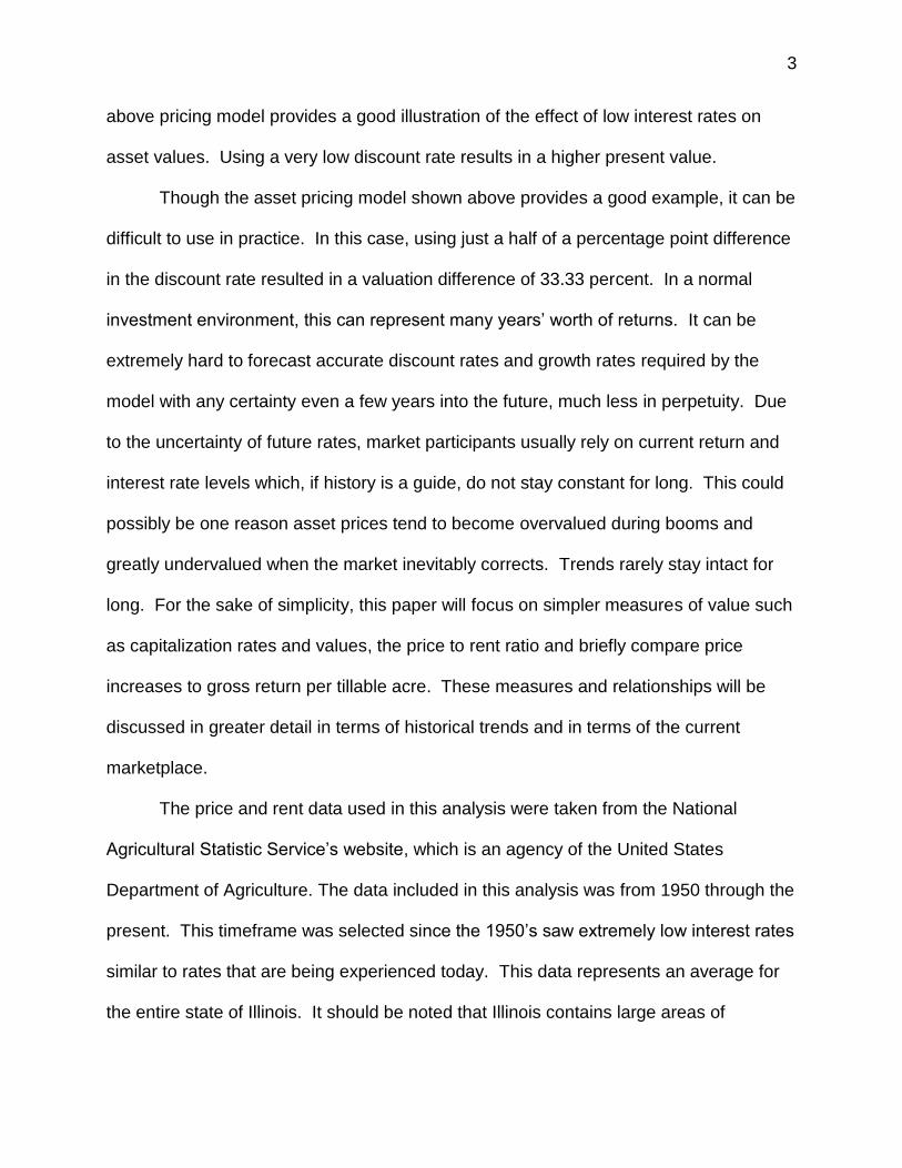
above pricing model provides a good illustration of the effect of low interest rates on
asset values. Using a very low discount rate results in a higher present value.
Though the asset pricing model shown above provides a good example, it can be
difficult to use in practice. In this case, using just a half of a percentage point difference
in the discount rate resulted in a valuation difference of 33.33 percent. In a normal
investment environment, this can represent many years’ worth of returns. It can be
extremely hard to forecast accurate discount rates and growth rates required by the
model with any certainty even a few years into the future, much less in perpetuity. Due
to the uncertainty of future rates, market participants usually rely on current return and
interest rate levels which, if history is a guide, do not stay constant for long. This could
possibly be one reason asset prices tend to become overvalued during booms and
greatly undervalued when the market inevitably corrects. Trends rarely stay intact for
long. For the sake of simplicity, this paper will focus on simpler measures of value such
as capitalization rates and values, the price to rent ratio and briefly compare price
increases to gross return per tillable acre. These measures and relationships will be
discussed in greater detail in terms of historical trends and in terms of the current
marketplace.
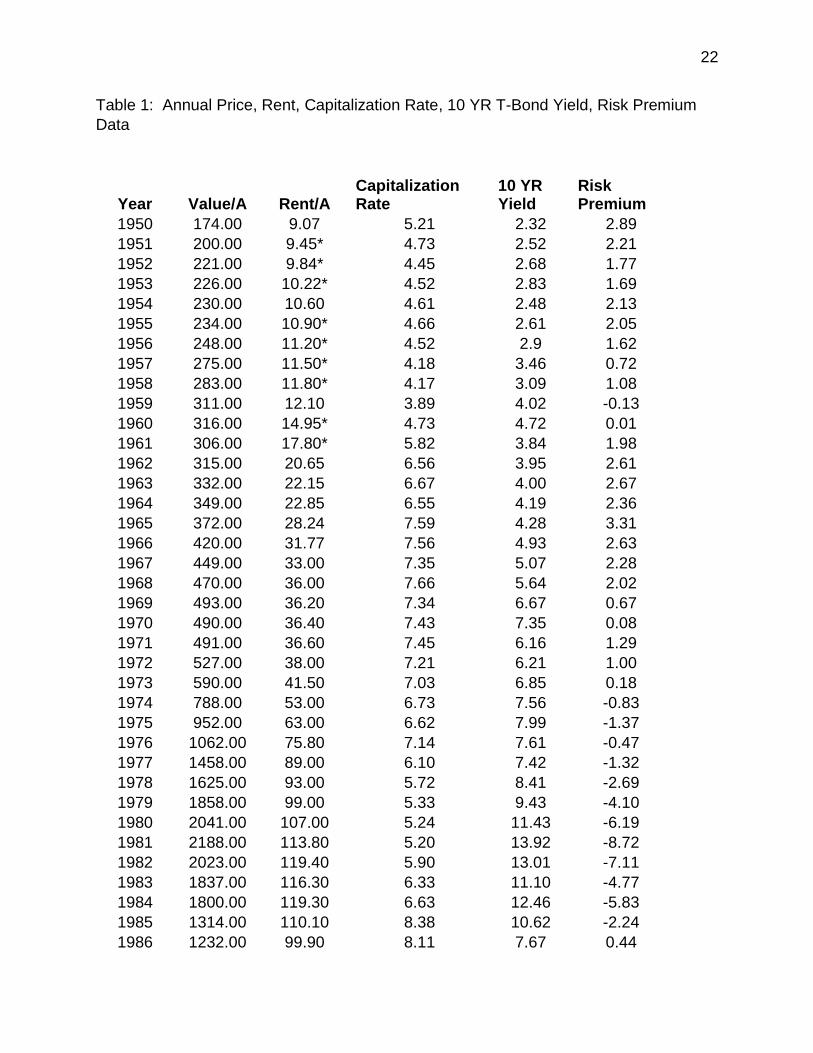
The price and rent data used in this analysis were taken from the National
Agricultural Statistic Service’s website, which is an agency of the United States
Department of Agriculture. The data included in this analysis was from 1950 through the
present. This timeframe was selected since the 1950’s saw extremely low interest rates
similar to rates that are being experienced today. This data represents an average for
the entire state of Illinois. It should be noted that Illinois contains large areas of
4
excellent quality soils but also areas that are very poor. It is unfortunate that accurate
farm rental data does not exist at the county level or even regional level prior to 1990
when much more accurate rent data started being collected, as this might reveal areas
prone to long term price discrepancies and abnormalities. Also, rent data was not
available for every year prior to 1964, only, 1959, 1954, and 1950. Values for the
missing years were estimated and are shown in the table containing rent data in the
appendix. Changes in price and rent values over this time period were fairly mild and
constant so the estimated values are believed to be accurate. Interest rate data on
Ten-Year Treasury Notes are constant maturity rates and are taken from the Federal
Reserve Bank of St. Louis’s website. The 2016 value is through the end of September.
5
CHAPTER 2
TREND CHANGES IN LAND VALUES
Farmland prices have seen a dramatic increase in recent years. This rise has
closely resembled the last period of rapidly increasing prices in the 1970’s which gave
way to the bust of the 1980’s. During this period, land prices fell nearly 50 percent
causing a wave of farm bankruptcies and foreclosures across the country. As shown in
Figure 1, land prices began accelerating again in 2004. From this date, values
increased from $2650 per acre to a peak of $7700 per acre in 2014. This represents an
increase of 290 percent or approximately 9 percent per year over the 10-year period
from 2004 through 2014. This rapid increase bears a similar resemblance to the
abnormally fast price increases of the 1970’s. During the 8-year period from 1973
through 1981 prices increased 370 percent or 17.56 percent per year on average.
Figure 1. Nominal Illinois Land Values and Cash Rents 1950-2016 Source: National Agricultural Statistics Service
0.00
50.00
100.00
150.00
200.00
250.00
0.00
1000.00
2000.00
3000.00
4000.00
5000.00
6000.00
7000.00
8000.00
9000.00
19
50
19
52
19
54
19
56
19
58
19
60
19
62
19
64
19
66
19
68
19
70
19
72
19
74
19
76
19
78
19
80
19
82
19
84
19
86
19
88
19
90
19
92
19
94
19
96
19
98
20
00
20
02
20
04
20
06
20
08
20
10
20
12
20
14
20
16
Value/A Rent/A
6
Figure 1 also contains a graph of cash rent values received by landowners over
the same time frame mentioned previously. It very closely resembles the graph of
farmland prices with rents rising much faster than historical averages over similar time
periods. Cash rents provide one of the most important measures of farmland returns.
Using cash rent data, it is possible to derive several valuation methods which will be
discussed shortly. Recently, land values have begun to pull back from their all-time
high as the future earnings potential of farmland has started to be called into question.
However, it is too early to declare this a trend of falling prices.
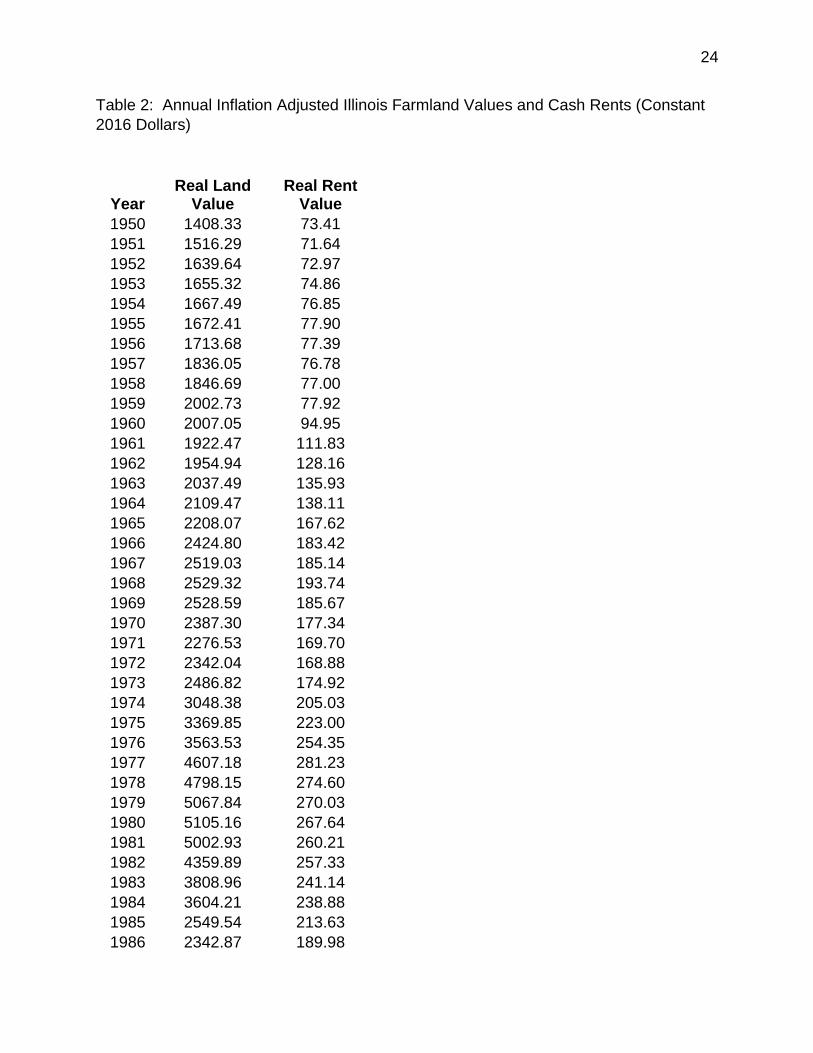
Figure 2. Real Land Values and Cash Rents 1950-2016 (Inflation Adjusted) Source: National Agricultural Statistics Service, US Bureau of Economic Analysis
Figure 2 shows a graph of real (inflation adjusted) Illinois farmland values in
constant 2016 dollars. What is most startling about this graph is how the boom of the
1970’s ended. In nominal terms, it has already been shown that when this bubble
popped, prices fell approximately 50 percent. However, in real terms after adjusting for
0.00
1000.00
2000.00
3000.00
4000.00
5000.00
6000.00
7000.00
8000.00
9000.00
0.00
50.00
100.00
150.00
200.00
250.00
300.00
19
50
19
52
19
54
19
56
19
58
19
60
19
62
19
64
19
66
19
68
19
70
19
72
19
74
19
76
19
78
19
80
19
82
19
84
19
86
19
88
19
90
19
92
19
94
19
96
19
98
20
00
20
02
20
04
20
06
20
08
20
10
20
12
20
14
20
16
Real Rent Value Real Land Value
7
inflation, prices fell from a peak of $5105 in 1980 to a low of $2133 in 1987,
representing a decline of 58 percent. Remarkably, land values only eclipsed their 1980
high in 2008, 28 years later. Solely from a price appreciation standpoint, excluding
rents received, an unfortunate farmland buyer at the peak of the bubble in 1980 saw
real annual compounded returns through 2016 of only 1.05 percent per year. If the
initial purchase had occurred at the low in 1987, the buyer would have realized real
annual returns after inflation of 4.4 percent per year through the present. For
perspective, over the entire 66-year period in question, beginning in 1950, a farmland
buyer would have realized real average returns after inflation of approximately 2.93
percent per year.
Figure 3 and Figure 4 provide a summary of the returns to farmland ownership
over various time periods presented in nominal terms and also inflation adjusted values
given in 2016 dollars. The returns are separated to distinguish returns from cash rent
as a percentage of land value and the return from price appreciation in terms of
percentage change from a year earlier. These values are summed to provide the total
return to farmland ownership. The entire 66-year period has been divided into periods
where different trends appear to exist since the rates of return vary greatly over the
entire time horizon of this study.
The period of 1950 through 1972 was characterized by gradual, steady
increases in land prices providing returns very similar to the returns realized by holding
farmland over the entire 66-year period. The boom period of 1970 through 1981 saw
returns far above that of the historical average as land prices appreciated on average by
17.5 percent per year. Following this boom period, land prices collapsed during the
8
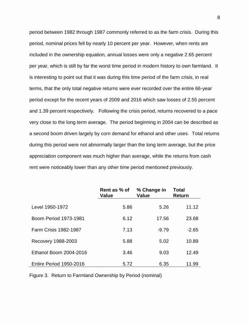
period between 1982 through 1987 commonly referred to as the farm crisis. During this
period, nominal prices fell by nearly 10 percent per year. However, when rents are
included in the ownership equation, annual losses were only a negative 2.65 percent
per year, which is still by far the worst time period in modern history to own farmland. It
is interesting to point out that it was during this time period of the farm crisis, in real
terms, that the only total negative returns were ever recorded over the entire 66-year
period except for the recent years of 2009 and 2016 which saw losses of 2.55 percent
and 1.39 percent respectively. Following the crisis period, returns recovered to a pace
very close to the long term average. The period beginning in 2004 can be described as
a second boom driven largely by corn demand for ethanol and other uses. Total returns
during this period were not abnormally larger than the long term average, but the price
appreciation component was much higher than average, while the returns from cash
rent were noticeably lower than any other time period mentioned previously.
Rent as % of Value
% Change in Value
Total Return
Level 1950-1972 5.86 5.26 11.12
Boom Period 1973-1981 6.12 17.56 23.68
Farm Crisis 1982-1987 7.13 -9.79 -2.65
Recovery 1988-2003 5.88 5.02 10.89
Ethanol Boom 2004-2016 3.46 9.03 12.49
Entire Period 1950-2016 5.72 6.35 11.99
Figure 3. Return to Farmland Ownership by Period (nominal)
9
Rent as % of Value
% Change in Value
Total Return
Level 1950-1972 5.86 2.42 8.29
Boom Period 1973-1981 6.12 9.2 15.33
Farm Crisis 1982-1987 7.13 -12.87 -5.73
Recovery 1988-2003 5.88 2.62 8.5
Ethanol Boom 2004-2016 3.46 6.92 10.38
Entire Period 1950-2016 5.72 2.93 8.57
Figure 4. Return to Farmland Ownership by Period (inflation adjusted) Given the above data, farmland purchases appear to provide fairly reliable
returns of around 12 percent per year or 8.6 percent yearly after inflation. Since
farmland is often considered an alternative investment, it is prudent to measure its
returns against another benchmark commonly used as an investment vehicle such as
the S&P 500. Using data from the website of economist Robert Schiller, annual returns
from an investment in the S&P 500 since 1950 including dividends have been 11.03
percent in nominal terms and 7.23 percent when adjusting for inflation. This compares
very closely with total farmland returns of 11.99 percent and 8.57 percent after inflation.
While farmland ownership appears to have a slight advantage, it is important to
remember that these returns do not include expenses that would normally be incurred
by landlords such as property taxes and improvements and maintenance of the land
which may shave approximately 1 percentage point off of returns. Considering the
above data, it is safe to conclude these two asset classes have provided similar returns
since 1950. Farmland could also be considered the more stable investment of the two
10
since the biggest yearly decline was only 27 percent which occurred in 1985 while the
largest yearly decline for the S&P 500 was 38% in 2009.
It should be noted that while rents and land values appear to be very closely
correlated, rents are based mostly on short term farm profitability and earnings, while
land values are influenced by many forces not directly related to farm profitability, such
as interest rates and inflation, and represent many years of future expectations. Baker
et al, 2013 have demonstrated that farmland can be added to a diversified portfolio and
achieve the goals of acting as an inflation hedge and providing returns comparable to
an investment in the S&P 500 over time. This increases the demand for farmland from
investors without an agricultural background who are looking for safety in times of
economic uncertainty. This also suggests that farmland prices are influenced by larger
outside market forces not directly pertaining to farm profitability which need to be
considered.
11
CHAPTER 3
VALUATION METHODS
While the returns to farmland ownership from cash rent have already briefly been
discussed, this ratio deserves closer examination. This ratio of cash rent to farmland
values is also known as the capitalization ratio, representing the rate of return to
farmland given the present market price.
Figure 5. Farmland Capitalization Rates and 10 Yr T-Bond Yields 1950-2016 Source: Bond yield data taken from St. Louis Federal Reserve Bank Figure 5 shows the capitalization rates for Illinois farmland over time and also the
yearly average rate of return on 10 year United States Treasury Bonds. While there is
0.00
2.00
4.00
6.00
8.00
10.00
12.00
14.00
16.00
19
50
19
52
19
54
19
56
19
58
19
60
19
62
19
64
19
66
19
68
19
70
19
72
19
74
19
76
19
78
19
80
19
82
19
84
19
86
19
88
19
90
19
92
19
94
19
96
19
98
20
00
20
02
20
04
20
06
20
08
20
10
20
12
20
14
20
16
Capitalization Rate 10 yr Yield
12
definitely a relationship between capitalization rates and bond yields, it is by no means
perfect.
Since many studies of farmland values tend to compare capitalization rates to
10-year treasury yields, it is reasonable to assume there would be a strong correlation
between the two. As shown in Figure 5, this has largely been the case since 1950. The
biggest exception occurred during the period of the farm crisis. Prior to 1980, interest
rates had seen a gradual, steady increase from a low of around 2 percent in the 1950’s
rising to the mid 7 percent range by the middle of the 1970’s. Capitalization rates
followed a similar trajectory during this time period, rising higher than interest rates at
times but then converging by the mid 1970’s. Interest rates then began to increase at a
much faster pace reaching a high of nearly 14 percent by 1981. Capitalization rates
and interest rates become very disjointed during this time frame as capitalization rates
actually fall while interest rates peak.
Shown in figure 6 is the spread between capitalization rates and interest rates. It
is easy to see the time period in which the spread became very negative. Farmland
prices were rising very quickly during the 1970’s, likely quicker than what was justified
by fundamentals. When interest rates began to increase very rapidly in the late 1970’s
land values couldn’t fall fast enough to keep the spread within its’ historical range. It
took several years for land prices to begin to fall which brought capitalization rates back
in line with interest rates by 1985.
This lag was probably due to the limited liquidity commonly associated with the
farmland market. It has been established in a study by Johnson of the University of
Nebraska 2010, that the farmland turnover rate generally runs less than 3 percent per
13
year. Given these liquidity issues, it is evident how market discrepancies can occur
from time to time.
Figure 6. Farmland Capitalization Rates Less 10-Yr. Treasury Yields 1950-2016
As interest rates have steadily trended lower since the mid 1980’s, capitalization
rates have closely followed and converged in 1987. This marks the exact low in the
farmland market with prices steadily rising since. The spread has remained in a
reasonable range of plus or minus 1.5 percent. As interest rates have trended lower,
farmland prices have trended higher. This fits well with the example using the
capitalization model shown on page 2. As interest rates have decreased, the discount
rate used for the model has also decreased which results in an increase in the current
value of the asset. With current 10-year treasury yields bouncing around the 1.5 – 2
-10.00
-8.00
-6.00
-4.00
-2.00
0.00
2.00
4.00
19
50
19
52
19
54
19
56
19
58
19
60
19
62
19
64
19
66
19
68
19
70
19
72
19
74
19
76
19
78
19
80
19
82
19
84
19
86
19
88
19
90
19
92
19
94
19
96
19
98
20
00
20
02
20
04
20
06
20
08
20
10
20
12
20
14
20
16
14
percent range, it becomes evident that capital asset prices remain supported at very
high levels.
Figure 7. Capitalized Values and Actual Prices 1950-2016
Capitalized values are another way in which farmland prices are often measured.
A capitalized value is a simple capitalization model where cash rent is divided by an
interest rate, in this case, 10-year treasury yields. Figure 7 shows a graph of
capitalized values plotted along with actual farmland prices since 1950. Throughout
history, actual prices have tracked capitalized values fairly closely, except several years
immediately preceding the farm crisis, and several years during the first half of the farm
crisis. The year 1981 marked the largest divergence with an actual farmland price of
0.00
2000.00
4000.00
6000.00
8000.00
10000.00
12000.00
14000.00
19
50
19
52
19
54
19
56
19
58
19
60
19
62
19
64
19
66
19
68
19
70
19
72
19
74
19
76
19
78
19
80
19
82
19
84
19
86
19
88
19
90
19
92
19
94
19
96
19
98
20
00
20
02
20
04
20
06
20
08
20
10
20
12
20
14
20
16
Value/A capitalized value
15
$2188 and a capitalized value of $817. This should have provided a clear warning sign
that underlying fundamentals did not support such high land prices. Following this
divergence, these two values once again converged in the late 1980’s as land prices fell
dramatically. Beginning in 2011, when interest rates fell below 3 percent for the first
time since 1956, capitalized values have remained dramatically higher than actual land
prices. Capitalized values have been very volatile over the last 5 years. A difference in
the interest rate of 0.81% from 2014 through 2016 has caused capitalized values to
jump by $3,543 per acre. Throughout the first three quarters of 2016, actual prices
remained $5,316 below their capitalized value, the largest occurrence in this data set.
This is another prime example of how volatile markets can become during periods of
ultra-low interest rates. This large price difference can probably be attributed to the
belief of market participants that rates will not stay this low for much longer, or that the
cash rental portion of the equation is likely to fall which would also lead to lower
capitalized values going forward.
Another common ratio used to measure the relationship between land values and
the income they produce is the price to cash rent ratio. It is simply calculated by
dividing the price of land by its earnings, or cash rent received for that specific year. It
is very similar to the price to earnings ratio used by investors in the stock markets. A
price to cash rent ratio of 15 means an investor is willing to pay 15 dollars for every 1
dollar of cash rental income.
The price to cash rent ratio has an average value of 19.5 since 1950. The lowest
value of 11.93 was recorded in 1985, while the highest value of 33.64 was recorded this
year, in 2016. At the peak of the farmland price bubble, the price to rent ratio reached a
16
peak of nearly 20, very close to its’ historical average before falling to its low. The low
of 1985 coincided very closely with the low in the farmland market after the bubble of
the 1970’s ended. It has been on an upward trajectory ever since.
Figure 8. Price to Cash Rent Ratio for Illinois 1950-2016
This rise in the price to cash rent ratio has certainly been caused by declining
interest rates. Falling interest rates lead to a lower opportunity cost of capital,
increasing investors’ willingness to pay more for each dollar of current earnings.
Current price to cash rent ratios in the lower 30’s, far above modern historical averages,
should certainly give prospective farmland buyers a reason to pause.
0
5
10
15
20
25
30
35
40
19
50
19
52
19
54
19
56
19
58
19
60
19
62
19
64
19
66
19
68
19
70
19
72
19
74
19
76
19
78
19
80
19
82
19
84
19
86
19
88
19
90
19
92
19
94
19
96
19
98
20
00
20
02
20
04
20
06
20
08
20
10
20
12
20
14
20
16
Price to Rent Ratio Average
17
The most important component supporting the earnings potential of farmland,
which to this point has not been discussed, is farm profitability. Rising farm profitability
over recent years has supported increasingly higher cash rents. One way to look at this
is through the trend in gross farm returns per tillable acre. This data was collected
through the Illinois Farm Business Farm Management Associations’ website from
various Farm Income and Production Reports, published annually by the association.
Data was only available from 1994 through 2015. Older data was not included because
changes in record keeping procedures would not have allowed for an apple to apples
comparison. Gross returns per tillable acre were used before subtracting any expenses
since these are the earnings that support cash rent payments.
Figure 9. Illinois Gross Farm Returns Per Acre and Cash Rents 1994-2016 Source: Illinois Farm Business Farm Management Association
0.00
50.00
100.00
150.00
200.00
250.00
0
100
200
300
400
500
600
700
800
900
Gross farm returns Cash Rent
18
Figure 9 contains a graph of gross farm returns per tillable acre and cash rents.
From 1994 through 2004, gross returns and cash rents followed similar trends of slow,
gradual increases. After 2004, gross farm returns began to rise at a faster pace. The
graph shows a noticeable lag in the acceleration of cash rents. It wasn’t until
approximately 2007 that cash rents began increasing at a faster pace. Prior to 2007,
cash rent increases had averaged just 2.22 percent per year. From 2007 through 2015,
cash rent has increased at a much faster 6.4 percent per year. Also, notice how gross
farm returns peaked with a high of $851 in 2012 and have fallen 30 percent through the
most recent data available in 2015. Cash rents on the other hand have continued to
climb well past 2012 and have only dropped a few dollars an acre. This provided
another good illustration of the lags that can occur in the farmland market.
Figure 10. Proportion of Gross Returns Paid for Cash Rent 1994-2015
Benjamin W. Johnson [email protected] Southern Illinois University Carbondale Bachelor of Science, Plant and Soil Science, May 2011 Research Paper Title: An Analysis of Historical Illinois Farmland Valuations Major Professor: Dr. Ira Altman