An Efficient ADMM Algorithm for MultidimensionalAnisotropic Total Variation Regularization Problems

Sen Yang1,2, Jie Wang1,2, Wei Fan3, Xiatian Zhang3, Peter Wonka2, Jieping Ye1,2

1Center for Evolutionary Medicine and Informatics, The Biodesign Institute,2Computer Science and Engineering,Arizona State University, Tempe, USA

{senyang, jie.wang.2, peter.wonka, jieping.ye}@asu.edu3Huawei Noah’s Ark Lab, Hong Kong, China

{david.fanwei, zhangxiatian}@huawei.com

ABSTRACTTotal variation (TV) regularization has important applica-tions in signal processing including image denoising, imagedeblurring, and image reconstruction. A significant chal-lenge in the practical use of TV regularization lies in the non-differentiable convex optimization, which is difficult to solveespecially for large-scale problems. In this paper, we pro-pose an efficient alternating augmented Lagrangian method(ADMM) to solve total variation regularization problem-s. The proposed algorithm is applicable for tensors, thusit can solve multidimensional total variation regularizationproblems. One appealing feature of the proposed algorithmis that it does not need to solve a linear system of equa-tions, which is often the most expensive part in previousADMM-based methods. In addition, each step of the pro-posed algorithm involves a set of independent and smallerproblems, which can be solved in parallel. Thus, the pro-posed algorithm scales to large size problems. Furthermore,the global convergence of the proposed algorithm is guaran-teed, and the time complexity of the proposed algorithm isO(dN/ϵ) on a d-mode tensor with N entries for achieving anϵ-optimal solution. Extensive experimental results demon-strate the superior performance of the proposed algorithmin comparison with current state-of-the-art methods.

Categories and Subject DescriptorsH.2.8 [Database Management]: Database Applications—Data Mining

General TermsAlgorithms

KeywordsMultidimensional total variation, ADMM, parallel comput-ing, large scale

Permission to make digital or hard copies of all or part of this work for personal orclassroom use is granted without fee provided that copies are not made or distributedfor profit or commercial advantage and that copies bear this notice and the full cita-tion on the first page. Copyrights for components of this work owned by others thanACM must be honored. Abstracting with credit is permitted. To copy otherwise, or re-publish, to post on servers or to redistribute to lists, requires prior specific permissionand/or a fee. Request permissions from permissions@acm.org.KDD’13 August 11–14, 2013, Chicago, Illinois, USA.Copyright 2013 ACM 978-1-4503-2174-7/13/08 ...$15.00.

1. INTRODUCTIONThe presence of noise in signals is unavoidable. To re-

cover original signals, many noise reduction techniques havebeen developed to reduce or remove the noise. Noisy sig-nals usually have high total variation (TV). Several totalvariation regularization approaches have been developed toexploit the special properties of noisy signals and they havebeen widely used in noise reduction in signal processing. Thetotal variation model was first introduced by Rudin, Osherand Fatemi in [19] as a regularization approach to removenoise and handle proper edges in images. More recently,the total variation models have been applied successfully forimage reconstruction, e.g. Magnetic Resonance (MR) imagereconstruction [14, 17]. The wide range of applications in-cluding image restoration, image denoising and deblurring[1, 2, 14, 15, 22, 24], underscore its success in signal/imageprocessing. The discrete penalized version of the TV-basedimage denoising model solves an unconstrained convex min-imization problem of the following form:

minX

1

2∥X − Y ∥2F + λ∥X∥TV , (1)

where ∥ · ∥F is the Frobenius norm defined as ∥X∥F =√∑i,j x

2i,j , Y is the observed image, X is the desired un-

known image to be recovered, and ∥ · ∥TV is the discreteTV norm defined below. The nonnegative regularization pa-rameter λ provides a tradeoff between the noise sensitivityand closeness to the observed image. There are two popu-lar choices for the discrete TV norm: ℓ2-based isotropic TVdefined by

∥X∥TV =m∑i=1

n∑j=1

∥∇xi,j∥2, X ∈ ℜm×n,

and the ℓ1-based anisotropic TV defined by

∥X∥TV =m∑i=1

n∑j=1

∥∇xi,j∥1, X ∈ ℜm×n,

where ∇ denotes the forward finite difference operators onthe vertical and horizonal directions, i.e., ∇xi,j = (∇1xi,j ,∇2xi,j)

T :

∇1xi,j =

{xi,j − xi+1,j if 1 ≤ i < m0 if j = n

∇2xi,j =

{xi,j − xi,j+1 if 1 ≤ j < n0 if i = m.

Despite the simple form of the TV norm, it is a chal-lenge to solve TV-based regularization problems efficiently.One of the key difficulties in the TV-based image denoisingproblem is the nonsmoothness of the TV norm. Continuedresearch efforts have been made to build fast and scalablenumerical methods in the last few years. Existing methodsaim to balance the tradeoff between the convergence rateand the simplicity of each iterative step. For example, com-puting the exact optimal solution at each iteration leads to abetter convergence rate [20]. However, this usually requiresheavy computations, for instance, a large linear system ofequations. Simple methods with less computation efforts ateach iteration are more suitable for large-scale problems, butusually they have a slow convergence rate. To this end, wepropose a fast but simple ADMM algorithm to solve TV-based problems. The key idea of the proposed method is todecompose the large problem into a set of smaller and inde-pendent problems, which can be solved efficiently and exact-ly. Moreover, these small problems are decoupled, thus theycan be solved in parallel. Therefore, the proposed methodscales to large-size problems.Although the TV problems have been extensively stud-

ied for matrices (e.g. two-dimensional images), there is notmuch work on tensors, a higher-dimensional extension ofmatrices. Tensor data is common in real world applications,for instance, functional magnetic resonance imaging (fMRI)is a 3-mode tensor and a color video is a 4-mode tensor. An-other contribution of this paper is that the proposed ADMMalgorithm is designed to solve TV problems for tensors, e.g.,multidimensional TV problems. The 2D TV problem can besolved efficiently by a special case of the proposed algorith-m (for matrices). Our experiments show that the proposedmethod is more efficient than state-of-the-art approaches forsolving 2D TV problems. We further demonstrate the ef-ficiency of the proposed method for multidimensional TVproblems in image reconstruction, video denoising and im-age deblurring.

1.1 Related WorkDue to the nonsmoothness of the TV norm, solving large-

scale TV problems efficiently continues to be a challengingissue despite its simple form. In the past, considerable ef-forts have been devoted to develop an efficient and scalablealgorithm for TV problems. The 1D total variation, alsoknown as the fused signal approximator, has been widelyused in signal noise reduction. Liu et al. [16] propose an ef-ficient method to solve the fused signal approximator using awarm start technique. It has been shown to be very efficientin practice, though the convergence rate has not been estab-lished. Barabero and Sra [1] introduce a fast Newton-typemethod for 1D total variation regularization, and solve the2D total variation problem using the Dyktra’s method [7].Wahlberg et al. [23] propose an ADMM method to solve the1D total variation problem. A linear system of equation-s has to be solved at each iteration. Recently, a very fastdirect, noniterative, algorithm for 1D total variation prob-lem has been proposed in [8]. A dual-based approach tosolve the 2D total variation problems is introduced in [6].Beck and Teboulle [2] propose a fast gradient-based methodby combining the dual-based approach with the accelerationtechnique in Fast Iterative Shrinkage Thresholding Algorith-

Figure 1: Fibers of a 3-mode tensor: mode-1 fiber-s x:,j2,j3 , mode-2 fibers xj1,:,j3 , and mode-3 fibersxj1,j2,:(left to right).

m (FISTA) [3]. One potential drawback of the dual-basedapproaches is that it may not scale well. Goldstein and Osh-er introduce the split Bregman method to solve the 2D totalvariation problem, which is an application of split Bregmanmethod solving ℓ1 based problems. The total variation hasalso been widely used in Magnetic Resonance (MR) imagereconstruction [14, 17]. Ma et al.[17] introduce an operator-splitting algorithm (TVCMRI) to solve the MR image recon-struction problem. By combining the composite splitting al-gorithm [7] and the acceleration technique in FISTA, Huanget al. [14] propose an efficient MR image reconstruction al-gorithm called FCSA. We show that our proposed method ismuch more efficient than these methods for solving 2D TVproblems.

1.2 NotationWe use upper case letters for matrices, e.g. X, lower case

letters for the entries, e.g. xi,j , and bold lower case lettersfor vectors, e.g. x. The inner product in the matrix spaceis defined as ⟨X,Y ⟩ =

∑i,j xi,jyi,j . A d-mode tensor (or

d-order tensor) is defined as X ∈ ℜI1×I2×···×Id . Its entriesare denoted as xj1,...,jd , where 1 ≤ jk ≤ Ik, 1 ≤ k ≤ d.For example, 1-mode tensor is a vector, and 2-mode tensoris a matrix. xj1,...,ji−1,:,ji+1,...,jd denotes the mode-i fiberat {j1, . . . , ji−1, ji+1, . . . , jd}, which is the higher order ana-logue of matrix rows and columns (see Figure 1 for an il-lustration). The Frobenius norm of a tensor is defined as

∥X∥F = (∑

j1,j2,...,jdx2j1,j2,...,jd

)12 .The inner product in the

tensor space is defined as ⟨X ,Y⟩ =∑

j1,j2,...,jdxj1,j2,...,jd

yj1,j2,...,jd . For simplicity of notation, we use /{ji} to repre-sent the index set excluding ji, i.e., {j1, . . . , ji−1, ji+1, . . . , jd}.For instance,

∑j1,...,ji−1,ji+1,...,jd

can be simply written as∑/{ji}. In addition, we use a nonnegative superscript num-

ber to denote the iteration index, e.g., X k denotes the valueof X at the k-th iteration.

1.3 OrganizationWe present the multidimensional total variation regular-

ization problems and the proposed ADMM method in Sec-tion 2. One of the key steps in the proposed algorithm in-volves the solution of a 1D TV problem; we show how toestimate the active regularization parameter range for 1DTV problem in Section 3. We report empirical results inSection 4, and conclude this paper in Section 5.

2. THE PROPOSED ALGORITHM FORMULTIDIMENSIONAL TV PROBLEMS

We first introduce the multidimensional total variationregularization problems in Section 2.1. In Section 2.2, we

present the details of the proposed algorithm. The glob-al convergence is established in Section 2.3. Section 2.4presents the time complexity of the proposed algorithm.

2.1 The Multidimensional TV ProblemDenote Fi(X ) as the fused operator along the i-th mode

of X taking the form of

Fi(X ) =∑/{ji}

Ii−1∑ji=1

|xj1,...,ji,...,jd − xj1,...,(ji+1),...,jd |.

In the case of matrix, Fi(X) only involves the rows or column-s ofX. For example, F1(X) =

∑nj=1

∑m−1i=1 |xi,j−xi+1,j |, X ∈

ℜm×n. It is clear that the ℓ1-based anisotropic TV norm formatrices can be rewritten as

∑2i=1 Fi(X). The tensor is the

generalization of the matrix concept. We generalize the TVnorm for the matrix case to higher-order tensors by the fol-lowing tensor TV norm:

∥X∥TV =

d∑i=1

Fi(X ).

Based on the definition above, the TV-based denoising prob-lem for the matrix case can be generalized to tensors bysolving the following optimization problem:

minX

1

2∥Y − X∥2F + λ

d∑i=1

Fi(X ), (2)

where Y ∈ ℜI1×I2×...,×Id is the observed data representedas a tensor, X ∈ ℜI1×I2×...,×Id is the unknown tensor to beestimated,

∑di=1 Fi(X ) is the tensor TV norm, and λ is a

nonnegative regularization parameter. The tensor TV regu-larization encourages X to be smooth along all dimensions.

2.2 The Proposed AlgorithmWe propose to solve the multidimensional TV problem

(MTV) using ADMM [4]. ADMM decomposes a large glob-al problem into a series of smaller local subproblems, andcoordinates the local solutions to compute the globally op-timal solution. ADMM attempts to combine the benefits ofaugmented Lagrangian methods and dual decomposition forconstrained optimization problems [4]. The problem solvedby ADMM takes the following form:

minx,z

f(x) + g(z)

s.t. Ax+Bz = c,(3)

where x, z are unknown variables to be estimated.ADMM reformulates the problem using a variant of the

augmented Lagrangian method as follows:

Lρ(x, z, µ) = f(x)+g(z)+µT (Ax+Bz− c)+ρ

2∥Ax+Bz− c∥2

with µ being the augmented Lagrangian multiplier, and ρbeing the nonnegative penalty parameter (or dual updatelength). ADMM solves the original constrained problem byiteratively minimizing Lρ(x, z, µ) over x, z, and updating µaccording to the following update rule:

xk+1 =argminx

Lρ(x, zk, µk)

zk+1 =argminz

Lρ(xk+1, z, µk)

µk+1 =µk + ρ(Axk+1 +Bzk+1 − c).

Consider the unconstrained optimization problem in (2),which can be reformulated as the following constrained op-timization problem:

minX ,Zi

1

2∥Y − X∥2F + λ

d∑i=1

Fi(Zi)

s.t. X = Zi, for 1 ≤ i ≤ d,

(4)

where Zi, 1 ≤ i ≤ d are slack variables. The optimizationproblem in (4) can be solved by ADMM. The augmentedLagrangian of (4) is given by

L(X ,Zi,Ui) =1

2∥Y − X∥2F + λ

d∑i=1

Fi(Zi)+

d∑i=1

⟨Ui,Zi −X⟩+ρ

2

d∑i=1

∥Zi −X∥2F .

(5)

Applying ADMM, we carry out the following steps at eachiteration:Step 1 Update X k+1 with Zk

i and Uki fixed:

X k+1 =argminX

1

2∥Y − X∥2F −

d∑i=1

⟨Uki ,X⟩

+ρ

2

d∑i=1

∥Zki −X∥2F .

(6)

The optimal solution is given by

X k+1 =Y +

∑di=1(U

ki + ρZk

i )

1 + dρ. (7)

Step 2 Compute Zk+1i , i = 1, · · · , d with X k+1, and Uk

i , i =1, · · · , d fixed:

{Zk+1i } = argmin

{Zi}

ρ

2

d∑i=1

∥Zi −X k+1∥2F +d∑

i=1

⟨Uki ,Zi⟩

+ λ

d∑i=1

Fi(Zi),

(8)

where {Zi} denotes the set {Z1, . . . ,Zd}. This problem isdecomposable, i.e., we can solve Zk+1

i , 1 ≤ i ≤ d separately,

Zk+1i = argmin

Zi

ρ

2∥Zi −X k+1∥2F + ⟨Uk

i ,Zi⟩+ λFi(Zi),

which can be equivalently written as

Zk+1i = argmin

Zi

1

2∥Zi − Ti∥2F +

λ

ρFi(Zi) (9)

with Ti = − 1ρUki + X k+1. The problem in (9) is decompos-

able for different mode-i fibers. Denote zj1,...,ji−1,:,ji+1,...,jd

as a mode-i fiber to be estimated, which is a vector of Iilength. For simplicity, we use v to represent the vectorzj1,...,ji−1,:,ji+1,...,jd . Then, (9) can be decomposed into aset of independent and much smaller problems:

vk+1 = argminv

1

2∥v − t∥2 + λ

ρ

Ii−1∑i=1

|vi − vi+1|,

∀j1, . . . , ji−1, ji+1, . . . , jd,

(10)

where t is the corresponding mode-i fiber of Ti. (10) isthe formulation of 1D total variation regularization problem,which can be solved exactly and very efficiently [8, 16].

The problem of computing Zk+1i , 1 ≤ i ≤ d in (8) is there-

fore decomposed into a set of much smaller problems of com-puting fibers. Each fiber problem is independent, enablingthat the whole set of problems can be computed in parallel.Step 3 Update Uk+1

i , i = 1, . . . , d:

Uk+1i = Uk

i + ρ(Zk+1i −X k+1). (11)

A summary of the proposed method is shown in Algorith-m 1 below.

Algorithm 1: The proposed ADMM algorithm formulti-dimensional total variationInput: Y, λ, ρOutput: XInitialization: Z0

i = X 0 ← Y,U0i ← 0;

doCompute X k+1 according to Eq. (7).Compute Zk+1

i , i = 1, . . . , d according to Eq. (9).Compute Uk+1

i , i = 1, . . . , d according to Eq. (11).Until Convergence;return X ;

The algorithm stops when the primal and dual residuals[4] satisfy a certain stopping criterion. The stopping crite-rion can be specified by two thresholds: absolute toleranceϵabs and relative tolerance ϵrel (see Boyd et al. [4] for moredetails). The penalty parameter ρ affects the primal and d-ual residuals, hence affects the termination of the algorithm.A large ρ tends to produce small primal residuals, but in-creases the dual residuals [4]. A fixed ρ (say 10) is commonlyused. But there are some schemes of varying the penalty pa-rameter to achieve better convergence. We refer interestedreaders to Boyd et al. [4] for more details.

Remark 1. We can add the ℓ1 regularization in the for-mulation of multidimensional TV problems for a sparse so-lution. The subproblem with ℓ1 regularization is called thefused signal approximator. The optimal solution can be ob-tained by first solving 1D total variation problem, then ap-plying soft-thresholding [11, 16].

2.3 Convergence AnalysisThe convergence of ADMM to solve the standard form (3)

has been extensively studied [4, 10, 13]. We establish theconvergence of Algorithm 1 by transforming the MTV prob-lem in (4) into a standard form (3), and show that the trans-formed optimization problem satisfies the condition neededto establish the convergence.Denote x as the vectorization of X , i.e., x = vec(X ) ∈ℜ

∏i Ii×1, y = vec(Y) ∈ ℜ

∏i Ii×1, z = [vec(Z1)

T , . . . , vec(Zd)T

]T ∈ ℜd∏

i Ii×1, f(x) = 12∥y − x∥22, and g(z) = λ

∑di=1 Fi(Zi).

Then the MTV problem in (4) can be rewritten as

minx,z

f(x) + g(z),

s.t. Ax− z = 0,(12)

where A = [I, . . . , I]T ∈ ℜd∏

i Ii×∏

i Ii , and I is the identitymatrix of size

∏i Ii ×

∏i Ii. The first and second steps

of Algorithm 1 are exactly the steps of updating x and z inthe standard form. Since f, g are proper, closed, and convex,and A is of column full rank, the convergence of Algorithm 1directly follows from the results in [4, 10, 13]. Moreover, an

O(1/k) convergence rate of Algorithm 1 can be establishedfollowing the conclusion in [13].

2.4 Time Complexity AnalysisThe first step of Algorithm 1 involves computations ofX k+1

i , i = 1, . . . , d. Computing X k+1i needs to compute∏

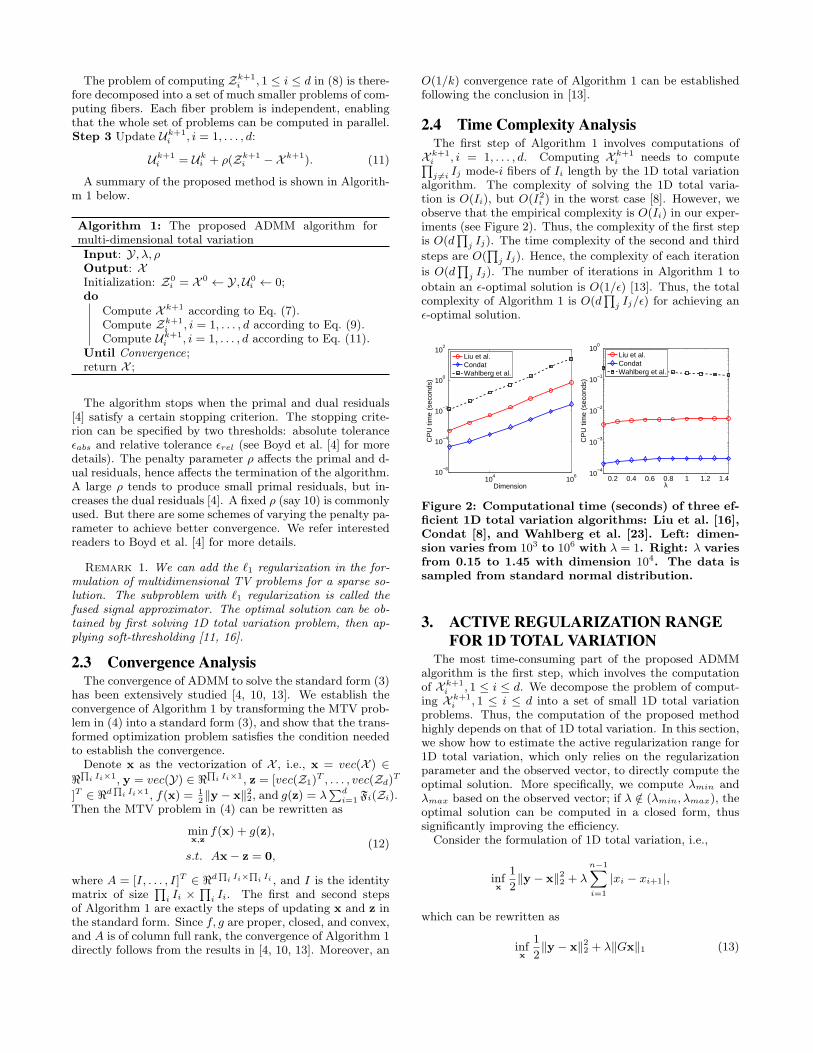
j =i Ij mode-i fibers of Ii length by the 1D total variationalgorithm. The complexity of solving the 1D total varia-tion is O(Ii), but O(I2i ) in the worst case [8]. However, weobserve that the empirical complexity is O(Ii) in our exper-iments (see Figure 2). Thus, the complexity of the first stepis O(d

∏j Ij). The time complexity of the second and third

steps are O(∏

j Ij). Hence, the complexity of each iteration

is O(d∏

j Ij). The number of iterations in Algorithm 1 to

obtain an ϵ-optimal solution is O(1/ϵ) [13]. Thus, the totalcomplexity of Algorithm 1 is O(d

∏j Ij/ϵ) for achieving an

ϵ-optimal solution.

104

106

10−6

10−4

10−2

100

102

Dimension

CP

U ti

me

(sec

onds

)

Liu et al.CondatWahlberg et al.

0.2 0.4 0.6 0.8 1 1.2 1.410

−4

10−3

10−2

10−1

100

λ

CP

U ti

me

(sec

onds

)

Liu et al.CondatWahlberg et al.

Figure 2: Computational time (seconds) of three ef-ficient 1D total variation algorithms: Liu et al. [16],Condat [8], and Wahlberg et al. [23]. Left: dimen-sion varies from 103 to 106 with λ = 1. Right: λ variesfrom 0.15 to 1.45 with dimension 104. The data issampled from standard normal distribution.

3. ACTIVE REGULARIZATION RANGEFOR 1D TOTAL VARIATION

The most time-consuming part of the proposed ADMMalgorithm is the first step, which involves the computationof X k+1

i , 1 ≤ i ≤ d. We decompose the problem of comput-ing X k+1

i , 1 ≤ i ≤ d into a set of small 1D total variationproblems. Thus, the computation of the proposed methodhighly depends on that of 1D total variation. In this section,we show how to estimate the active regularization range for1D total variation, which only relies on the regularizationparameter and the observed vector, to directly compute theoptimal solution. More specifically, we compute λmin andλmax based on the observed vector; if λ /∈ (λmin, λmax), theoptimal solution can be computed in a closed form, thussignificantly improving the efficiency.

Consider the formulation of 1D total variation, i.e.,

infx

1

2∥y − x∥22 + λ

n−1∑i=1

|xi − xi+1|,

which can be rewritten as

infx

1

2∥y − x∥22 + λ∥Gx∥1 (13)

in which y,x ∈ ℜn. G ∈ ℜ(n−1)×n encodes the structure ofthe 1D TV norm. We have

gi,j =

1 if j = i+ 1

−1 if j = i

0 otherwise.

(14)

3.1 The Dual ProblemBefore we derive the dual formualtion of problem in (13)

[5, 9], we first introduce some useful definitions and lemmas.

Definition 1. (Coercivity).[9] A function ϕ : ℜn → ℜis said to be coercive over a set S ⊂ ℜn if for every sequence{xk} ⊂ S

limk→∞

ϕ(xk) = +∞ whenever ∥xk∥ → +∞.

For S = ℜn, ϕ is simply called coercive.

Denote the objective function in problem (13) as:

f(x) =1

2∥y − x∥22 + λ∥Gx∥1. (15)

It is easy to see that f(x) is coercive. For each α ∈ ℜ, wedefine the α sublevel set of f(x) as Sα = {x : f(x) ≤ α}.Then we have the following lemma.

Lemma 1. For any α ∈ ℜ, the sublevel set Sα = {x :f(x) ≤ α} is bounded.

Proof. We prove the lemma by contradiction. Supposethere exists an α such that Sα is unbounded. Then we canfind a sequence {xk} ⊂ Sα such that limk→∞ ∥xk∥ =∞. Be-cause f(x) is coercive, we can conclude that limk→∞ f(xk) =+∞. However, since {xk} ⊂ Sα, we know f(xk) ≤ α for allk, which leads to a contradiction. Therefore, the proof iscomplete.

We derive the dual formulation of problem (13) via theSion’s Minimax Theorem [9, 21]. Let B = {x : y−λGT s, ∥s∥∞≤ 1} and x′ = argmaxx∈B f(x). Because B is compact, x′

must exist. Denote α′ = f(x′) and S ′ = Sα′ .

infx

1

2∥y − x∥22+λ∥Gx∥1 = inf

x∈S′

1

2∥y − x∥22 + λ∥Gx∥1

= infx∈S′

1

2∥y − x∥22 + λ sup

∥s∥∞≤1

⟨s, Gx⟩

= infx∈S′

sup∥s∥∞≤1

1

2∥y − x∥22 + λ⟨s, Gx⟩.

(16)

By Lemma 1, we know that S ′ is compact. Moreover, thefunction

1

2∥y − x∥22 + λ⟨s, Gx⟩

is convex and concave with respect to x and s respectively.Thus, by the Sion’s Minimax Theorem [21], we have

infx

1

2∥y − x∥22 + λ∥Gx∥1 (17)

= infx∈S′

sup∥s∥∞≤1

1

2∥y − x∥22 + λ⟨s, Gx⟩

= sup∥s∥∞≤1

infx∈S′

1

2∥y − x∥22 + λ⟨s, Gx⟩.

We can see that

x∗(s) = y − λGT s = argminx∈S′

1

2∥y − x∥22 + λ⟨s, Gx⟩ (18)

and thus

infx∈S′

1

2∥y − x∥22 + λ⟨s, Gx⟩ = −λ2

2∥GT s∥2 + λ⟨s, Gy⟩

=1

2∥y∥2 − λ2

2∥yλ−GT s∥2.

Therefore the primal problem (16) is transformed to its dualproblem:

sup∥s∥∞≤1

1

2∥y∥2 − λ2

2∥yλ−GT s∥2, (19)

which is equivalent to

mins∥yλ−GT s∥2 (20)

s.t. ∥s∥∞ ≤ 1.

3.2 Computing the Maximal Value for λ

Recall the definition of G in (14), it follows that GT hasfull column rank. Denote e = (1, · · · , 1)T ∈ ℜn, and thesubspace spanned by the rows of G and e as VGT and Ve.Clearly ℜn = VGT ⊕ Ve and VGT ⊥ Ve.

Let P = I − eeT

⟨e,e⟩ and P⊥ denote the projection operator

into VGT and Ve respectively. Therefore the equation

Py = GT s (21)

must have a unique solution for each y.Let Py = y, then it follows that

si = −i∑

j=1

yj , ∀i = 1, · · · , n− 1

and clearly sn−1 = −∑n−1

j=1 yj = yn since ⟨e, y⟩ = 0. Denote

λmax = ∥s∥∞ = max{|i∑

j=1

yj | : i = 1, · · · , n− 1}. (22)

From the above analysis, it is easy to see that when λ ≥λmax, there is an s∗ such that

Py

λ= GT s

∗and ∥s∗∥∞ ≤ 1.

According to (18), we have

x∗ = (P+P⊥)y−λGT s∗ = P⊥y =⟨e,y⟩⟨e, e⟩ e =

⟨e,y⟩n

e. (23)

The maximal value for λ has been studied in [16]. Howev-er, a linear system has to be solved. From (22), it is easy tosee that the maximal value can be obtained by a close formsolution. Thus, our approach is more efficient.

3.3 Computing the Minimum Value for λ

We rewrite the dual problem (19) as:

mins

1

2∥y − λGT s∥2 (24)

s.t. ∥s∥∞ ≤ 1.

Denote g(s) = 12∥y − λGT s∥2. The gradient of g(s) can

be found as: g′(s) = −λG(y − λGT s).

Let B∞ denote the unit∞ norm ball. We know that s∗ isthe unique optimal solution to the problem (24) if and onlyif

−g′(s∗) ∈ NB∞(s∗),

where NB∞(s∗) is the normal cone at s∗ with respect to B∞.Let I+(s) = {i : si = 1}, I−(s) = {i : si = −1}, andI◦(s) = {i : si ∈ (−1, 1)}. Assume d ∈ NB∞(s), then d canbe found as:

di ∈

[0,+∞), if i ∈ I+(s)(−∞, 0], if i ∈ I−(s)0, if i ∈ I◦(s)

Therefore the optimality condition can be expressed as:

s∗ = argmins

1

2∥y − λGT s∥2

if and only if

λG(y − λGT s∗) ∈ NB∞(s∗).

Because λ > 0, λG(y − λGT s) ∈ NB∞(s∗) is equivalent to

G(y − λGT s∗) ∈ NB∞(s∗). (25)

According to (18), we have

x∗1 =y1 + λs∗1

x∗i =yi − λ(s∗i−1 − s∗i ), for 1 < i < n (26)

x∗n =yn − λs∗n,

and

G(y − λGT s∗) =

x∗2 − x∗

1

...x∗n − x∗

n−1

. (27)

By (25) and (27), we have the following observations:

B1. If x∗i+1 > x∗

i , s∗i = 1;

B2. If x∗i+1 = x∗

i , s∗i ∈ [−1, 1];

B3. If x∗i+1 < x∗

i , s∗i = −1.

Notice that, from (26), we can estimate a range for everyx∗i , which is not necessarily the tightest one. In fact, we

have

x∗i ∈

{[yi − λ, yi + λ], if i ∈ {1, n}[yi − 2λ, yi + 2λ], otherwise.

(28)

Define

λmin = min

{|yi+1 − yi|

3, i ∈ {1, n− 1}; (29)

|yi+1 − yi|4

, i ∈ {2, . . . , n− 2}}.

It follows that when λ < λmin, the solution to (26) is fixedand can be found as:

s∗i = sign(yi+1 − yi), i = 1, . . . , n− 1. (30)

Then x∗i can be computed accordingly by (26).

4. RESULTSIn this section, we evaluate the efficiency of the proposed

algorithm on synthetic and real-word data, and show severalapplications of the proposed algorithm.

4.1 Efficiency ComparisonWe examine the efficiency of the proposed algorithm using

synthetic datasets on 2D and 3D cases. For the 2D case, thecompetitors include

• SplitBregman written in C1 [12];

• ADAL written in C faithfully based on the paper [18];

• The dual method in Matlab2 [2];

• Dykstra written in C [7];

For the 3D case, only the Dykstra’s method and the pro-posed method (MTV) are compared, since the other algo-rithms are designed specifically for the 2D case.

The experiments are performed on a PC with quad-coreIntel 2.67GHz CPU and 9GB memory. The code of MTV iswritten in C. Since the proposed method and the Dykstra’smethod can be implemented in parallel, we also comparetheir parallel versions implemented with OpenMP.

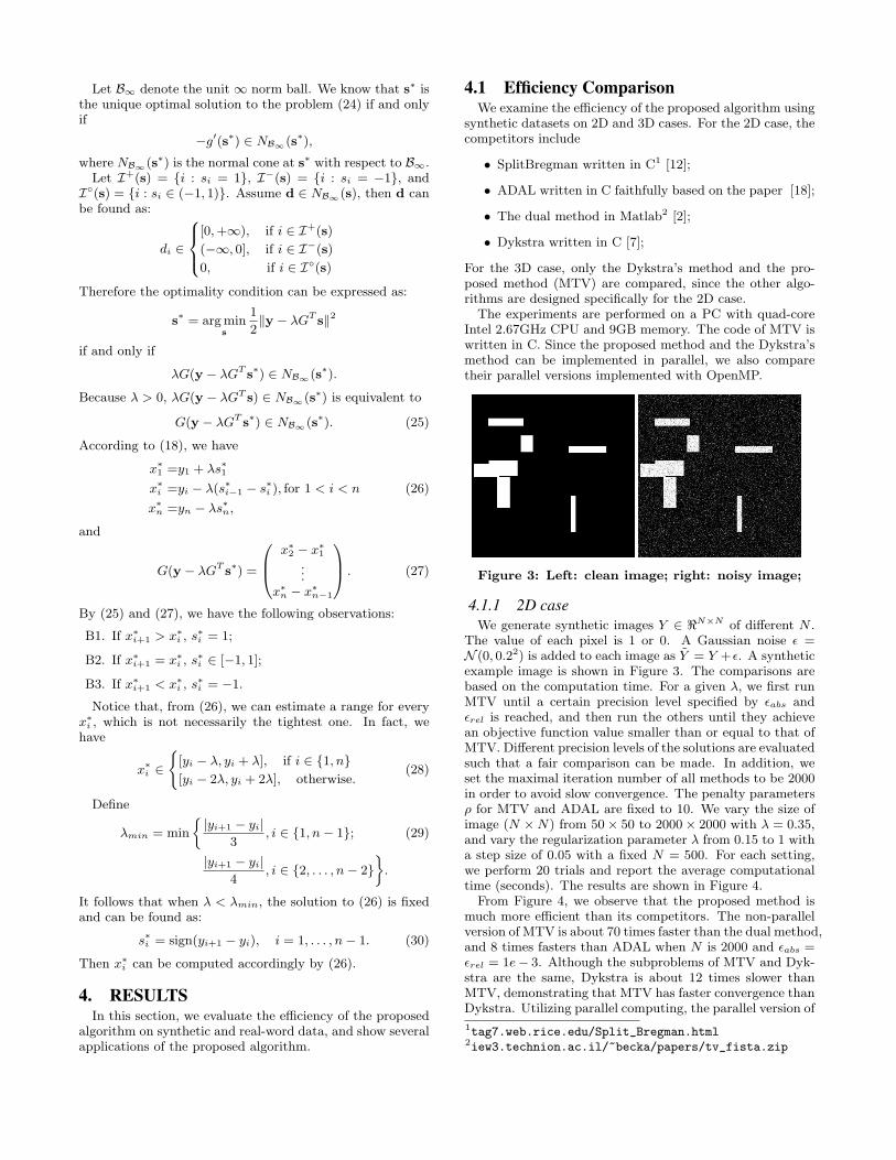
Figure 3: Left: clean image; right: noisy image;

4.1.1 2D caseWe generate synthetic images Y ∈ ℜN×N of different N .

The value of each pixel is 1 or 0. A Gaussian noise ϵ =N (0, 0.22) is added to each image as Y = Y +ϵ. A syntheticexample image is shown in Figure 3. The comparisons arebased on the computation time. For a given λ, we first runMTV until a certain precision level specified by ϵabs andϵrel is reached, and then run the others until they achievean objective function value smaller than or equal to that ofMTV. Different precision levels of the solutions are evaluatedsuch that a fair comparison can be made. In addition, weset the maximal iteration number of all methods to be 2000in order to avoid slow convergence. The penalty parametersρ for MTV and ADAL are fixed to 10. We vary the size ofimage (N ×N) from 50× 50 to 2000× 2000 with λ = 0.35,and vary the regularization parameter λ from 0.15 to 1 witha step size of 0.05 with a fixed N = 500. For each setting,we perform 20 trials and report the average computationaltime (seconds). The results are shown in Figure 4.

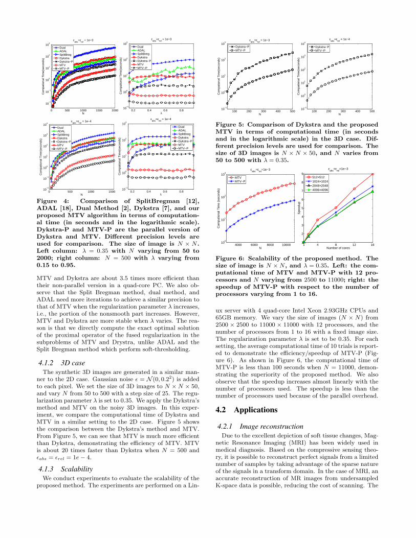
From Figure 4, we observe that the proposed method ismuch more efficient than its competitors. The non-parallelversion of MTV is about 70 times faster than the dual method,and 8 times fasters than ADAL when N is 2000 and ϵabs =ϵrel = 1e− 3. Although the subproblems of MTV and Dyk-stra are the same, Dykstra is about 12 times slower thanMTV, demonstrating that MTV has faster convergence thanDykstra. Utilizing parallel computing, the parallel version of

1tag7.web.rice.edu/Split_Bregman.html2iew3.technion.ac.il/~becka/papers/tv_fista.zip

0 500 1000 1500 2000

10−2

10−1

100

101

102

103

N

Com

patio

nal T

ime(

seco

nds)

εabs

=εrel

= 1e−3

DualADALSplitBregDykstraDykstra−PMTVMTV−P

0.2 0.4 0.6 0.810

−1

100

101

102

103

λ

Com

patio

nal T

ime(

seco

nds)

εabs

=εrel

= 1e−3

DualADALSplitBregDykstraDykstra−PMTVMTV−P

0 500 1000 150010

−2

10−1

100

101

102

103

104

N

Com

patio

nal T

ime(

seco

nds)

εabs

=εrel

= 1e−4

DualADALSplitBregDykstraDykstra−PMTVMTV−P

0.2 0.4 0.6 0.810

−1

100

101

102

103

λ

Com

patio

nal T

ime(

seco

nds)

εabs

=εrel

= 1e−4

DualADALSplitBregDykstraDykstra−PMTVMTV−P

Figure 4: Comparison of SplitBregman [12],ADAL [18], Dual Method [2], Dykstra [7], and ourproposed MTV algorithm in terms of computation-al time (in seconds and in the logarithmic scale).Dykstra-P and MTV-P are the parallel version ofDykstra and MTV. Different precision levels areused for comparison. The size of image is N × N .Left column: λ = 0.35 with N varying from 50 to2000; right column: N = 500 with λ varying from0.15 to 0.95.

MTV and Dykstra are about 3.5 times more efficient thantheir non-parallel version in a quad-core PC. We also ob-serve that the Split Bregman method, dual method, andADAL need more iterations to achieve a similar precision tothat of MTV when the regularization parameter λ increases,i.e., the portion of the nonsmooth part increases. However,MTV and Dykstra are more stable when λ varies. The rea-son is that we directly compute the exact optimal solutionof the proximal operator of the fused regularization in thesubproblems of MTV and Drystra, unlike ADAL and theSplit Bregman method which perform soft-thresholding.

4.1.2 3D caseThe synthetic 3D images are generated in a similar man-

ner to the 2D case. Gaussian noise ϵ = N (0, 0.22) is addedto each pixel. We set the size of 3D images to N ×N × 50,and vary N from 50 to 500 with a step size of 25. The regu-larization parameter λ is set to 0.35. We apply the Dykstra’smethod and MTV on the noisy 3D images. In this exper-iment, we compare the computational time of Dykstra andMTV in a similar setting to the 2D case. Figure 5 showsthe comparison between the Dykstra’s method and MTV.From Figure 5, we can see that MTV is much more efficientthan Dykstra, demonstrating the efficiency of MTV. MTVis about 20 times faster than Dykstra when N = 500 andϵabs = ϵrel = 1e− 4.

4.1.3 ScalabilityWe conduct experiments to evaluate the scalability of the

proposed method. The experiments are performed on a Lin-

100 200 300 400 50010

−1

100

101

102

103

N

Com

patio

nal T

ime(

seco

nds)

εabs

=εrel

= 1e−3

Dykstra−PMTV−P

100 200 300 400 50010

−1

100

101

102

103

104

N

Com

patio

nal T

ime(

seco

nds)

εabs

=εrel

= 1e−4

Dykstra−PMTV−P

Figure 5: Comparison of Dykstra and the proposedMTV in terms of computational time (in secondsand in the logarithmic scale) in the 3D case. Dif-ferent precision levels are used for comparison. Thesize of 3D images is N × N × 50, and N varies from50 to 500 with λ = 0.35.

4000 6000 8000 1000010

0

101

102

103

N

Com

putio

nal T

ime

(sec

onds

)

εabs

=εrel

=1e−3

MTVMTV−P

1 4 8 12 161

2

3

4

5

6

7

8

9

Number of cores

Spe

edup

εabs

=εrel

=1e−3

512×5121024×10242048×20484096×4096

Figure 6: Scalability of the proposed method. Thesize of image is N ×N , and λ = 0.35. Left: the com-putational time of MTV and MTV-P with 12 pro-cessors and N varying from 2500 to 11000; right: thespeedup of MTV-P with respect to the number ofprocessors varying from 1 to 16.

ux server with 4 quad-core Intel Xeon 2.93GHz CPUs and65GB memory. We vary the size of images (N × N) from2500 × 2500 to 11000 × 11000 with 12 processors, and thenumber of processors from 1 to 16 with a fixed image size.The regularization parameter λ is set to be 0.35. For eachsetting, the average computational time of 10 trials is report-ed to demonstrate the efficiency/speedup of MTV-P (Fig-ure 6). As shown in Figure 6, the computational time ofMTV-P is less than 100 seconds when N = 11000, demon-strating the superiority of the proposed method. We alsoobserve that the speedup increases almost linearly with thenumber of processors used. The speedup is less than thenumber of processors used because of the parallel overhead.

4.2 Applications

4.2.1 Image reconstructionDue to the excellent depiction of soft tissue changes, Mag-

netic Resonance Imaging (MRI) has been widely used inmedical diagnosis. Based on the compressive sensing theo-ry, it is possible to reconstruct perfect signals from a limitednumber of samples by taking advantage of the sparse natureof the signals in a transform domain. In the case of MRI, anaccurate reconstruction of MR images from undersampledK-space data is possible, reducing the cost of scanning. The

10

20

30

40

50

60

(a) Cardiac

10

20

30

40

50

60

(b) Brain

10

20

30

40

50

60

(c) Chest

10

20

30

40

50

60

(d) Artery

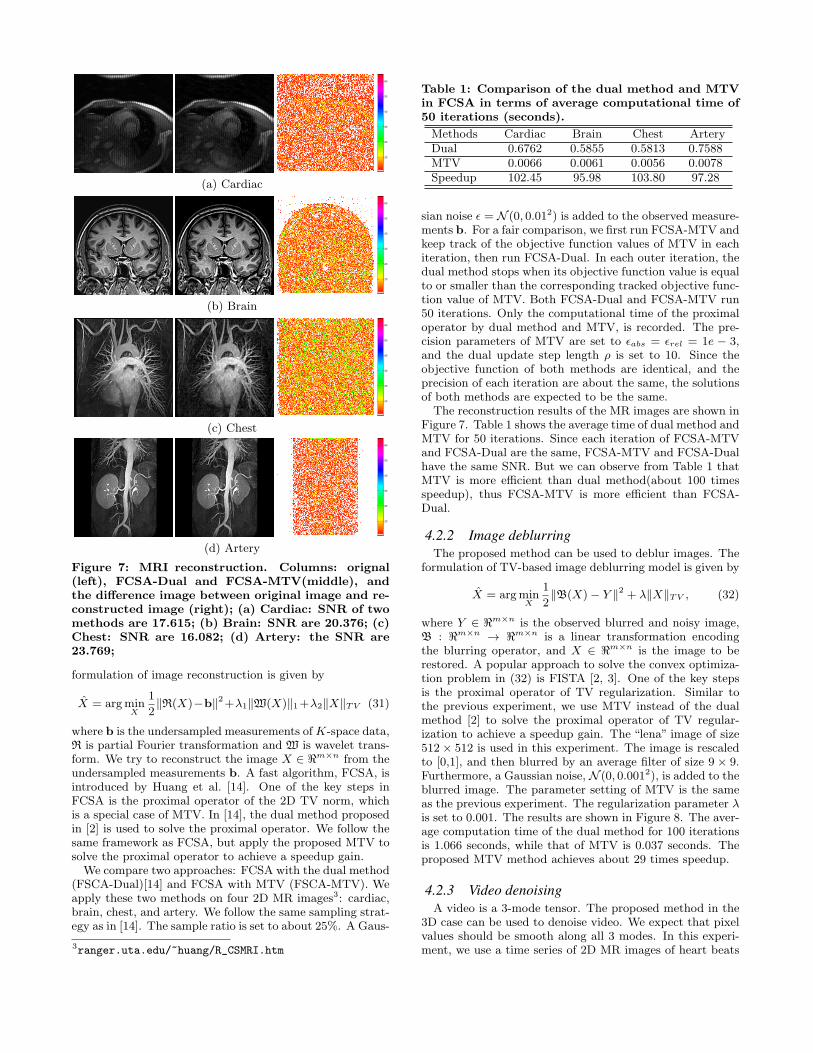
Figure 7: MRI reconstruction. Columns: orignal(left), FCSA-Dual and FCSA-MTV(middle), andthe difference image between original image and re-constructed image (right); (a) Cardiac: SNR of twomethods are 17.615; (b) Brain: SNR are 20.376; (c)Chest: SNR are 16.082; (d) Artery: the SNR are23.769;

formulation of image reconstruction is given by

X = argminX

1

2∥R(X)−b∥2+λ1∥W(X)∥1+λ2∥X∥TV (31)

where b is the undersampled measurements ofK-space data,R is partial Fourier transformation and W is wavelet trans-form. We try to reconstruct the image X ∈ ℜm×n from theundersampled measurements b. A fast algorithm, FCSA, isintroduced by Huang et al. [14]. One of the key steps inFCSA is the proximal operator of the 2D TV norm, whichis a special case of MTV. In [14], the dual method proposedin [2] is used to solve the proximal operator. We follow thesame framework as FCSA, but apply the proposed MTV tosolve the proximal operator to achieve a speedup gain.We compare two approaches: FCSA with the dual method

(FSCA-Dual)[14] and FCSA with MTV (FSCA-MTV). Weapply these two methods on four 2D MR images3: cardiac,brain, chest, and artery. We follow the same sampling strat-egy as in [14]. The sample ratio is set to about 25%. A Gaus-

3ranger.uta.edu/~huang/R_CSMRI.htm

Table 1: Comparison of the dual method and MTVin FCSA in terms of average computational time of50 iterations (seconds).

Methods Cardiac Brain Chest ArteryDual 0.6762 0.5855 0.5813 0.7588MTV 0.0066 0.0061 0.0056 0.0078Speedup 102.45 95.98 103.80 97.28

sian noise ϵ = N (0, 0.012) is added to the observed measure-ments b. For a fair comparison, we first run FCSA-MTV andkeep track of the objective function values of MTV in eachiteration, then run FCSA-Dual. In each outer iteration, thedual method stops when its objective function value is equalto or smaller than the corresponding tracked objective func-tion value of MTV. Both FCSA-Dual and FCSA-MTV run50 iterations. Only the computational time of the proximaloperator by dual method and MTV, is recorded. The pre-cision parameters of MTV are set to ϵabs = ϵrel = 1e − 3,and the dual update step length ρ is set to 10. Since theobjective function of both methods are identical, and theprecision of each iteration are about the same, the solutionsof both methods are expected to be the same.

The reconstruction results of the MR images are shown inFigure 7. Table 1 shows the average time of dual method andMTV for 50 iterations. Since each iteration of FCSA-MTVand FCSA-Dual are the same, FCSA-MTV and FCSA-Dualhave the same SNR. But we can observe from Table 1 thatMTV is more efficient than dual method(about 100 timesspeedup), thus FCSA-MTV is more efficient than FCSA-Dual.

4.2.2 Image deblurringThe proposed method can be used to deblur images. The

formulation of TV-based image deblurring model is given by

X = argminX

1

2∥B(X)− Y ∥2 + λ∥X∥TV , (32)

where Y ∈ ℜm×n is the observed blurred and noisy image,B : ℜm×n → ℜm×n is a linear transformation encodingthe blurring operator, and X ∈ ℜm×n is the image to berestored. A popular approach to solve the convex optimiza-tion problem in (32) is FISTA [2, 3]. One of the key stepsis the proximal operator of TV regularization. Similar tothe previous experiment, we use MTV instead of the dualmethod [2] to solve the proximal operator of TV regular-ization to achieve a speedup gain. The “lena” image of size512× 512 is used in this experiment. The image is rescaledto [0,1], and then blurred by an average filter of size 9 × 9.Furthermore, a Gaussian noise, N (0, 0.0012), is added to theblurred image. The parameter setting of MTV is the sameas the previous experiment. The regularization parameter λis set to 0.001. The results are shown in Figure 8. The aver-age computation time of the dual method for 100 iterationsis 1.066 seconds, while that of MTV is 0.037 seconds. Theproposed MTV method achieves about 29 times speedup.

4.2.3 Video denoisingA video is a 3-mode tensor. The proposed method in the

3D case can be used to denoise video. We expect that pixelvalues should be smooth along all 3 modes. In this experi-ment, we use a time series of 2D MR images of heart beats

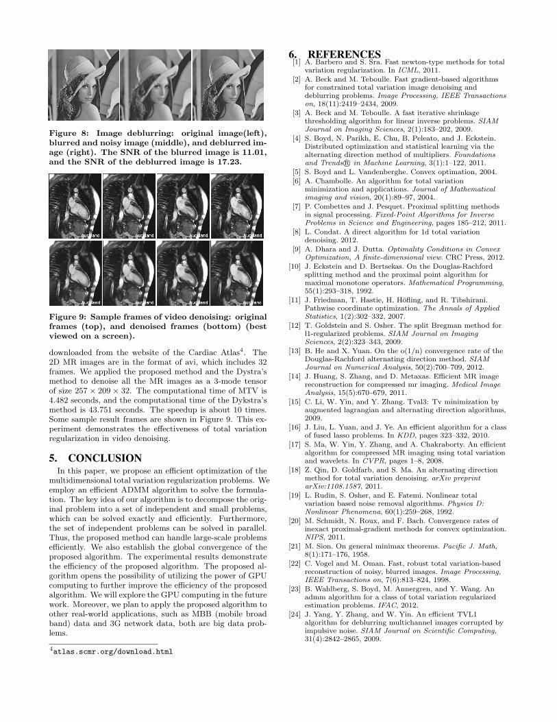
Figure 8: Image deblurring: original image(left),blurred and noisy image (middle), and deblurred im-age (right). The SNR of the blurred image is 11.01,and the SNR of the deblurred image is 17.23.

Figure 9: Sample frames of video denoising: originalframes (top), and denoised frames (bottom) (bestviewed on a screen).

downloaded from the website of the Cardiac Atlas4. The2D MR images are in the format of avi, which includes 32frames. We applied the proposed method and the Dystra’smethod to denoise all the MR images as a 3-mode tensorof size 257 × 209 × 32. The computational time of MTV is4.482 seconds, and the computational time of the Dykstra’smethod is 43.751 seconds. The speedup is about 10 times.Some sample result frames are shown in Figure 9. This ex-periment demonstrates the effectiveness of total variationregularization in video denoising.

5. CONCLUSIONIn this paper, we propose an efficient optimization of the

multidimensional total variation regularization problems. Weemploy an efficient ADMM algorithm to solve the formula-tion. The key idea of our algorithm is to decompose the orig-inal problem into a set of independent and small problems,which can be solved exactly and efficiently. Furthermore,the set of independent problems can be solved in parallel.Thus, the proposed method can handle large-scale problemsefficiently. We also establish the global convergence of theproposed algorithm. The experimental results demonstratethe efficiency of the proposed algorithm. The proposed al-gorithm opens the possibility of utilizing the power of GPUcomputing to further improve the efficiency of the proposedalgorithm. We will explore the GPU computing in the futurework. Moreover, we plan to apply the proposed algorithm toother real-world applications, such as MBB (mobile broadband) data and 3G network data, both are big data prob-lems.

4atlas.scmr.org/download.html

6. REFERENCES[1] A. Barbero and S. Sra. Fast newton-type methods for total

variation regularization. In ICML, 2011.[2] A. Beck and M. Teboulle. Fast gradient-based algorithms

for constrained total variation image denoising anddeblurring problems. Image Processing, IEEE Transactionson, 18(11):2419–2434, 2009.

[3] A. Beck and M. Teboulle. A fast iterative shrinkagethresholding algorithm for linear inverse problems. SIAMJournal on Imaging Sciences, 2(1):183–202, 2009.

[4] S. Boyd, N. Parikh, E. Chu, B. Peleato, and J. Eckstein.Distributed optimization and statistical learning via thealternating direction method of multipliers. Foundationsand Trends R⃝ in Machine Learning, 3(1):1–122, 2011.

[5] S. Boyd and L. Vandenberghe. Convex optimation, 2004.

[6] A. Chambolle. An algorithm for total variationminimization and applications. Journal of Mathematicalimaging and vision, 20(1):89–97, 2004.

[7] P. Combettes and J. Pesquet. Proximal splitting methodsin signal processing. Fixed-Point Algorithms for InverseProblems in Science and Engineering, pages 185–212, 2011.

[8] L. Condat. A direct algorithm for 1d total variationdenoising. 2012.

[9] A. Dhara and J. Dutta. Optimality Conditions in ConvexOptimization, A finite-dimensional view. CRC Press, 2012.

[10] J. Eckstein and D. Bertsekas. On the Douglas-Rachfordsplitting method and the proximal point algorithm formaximal monotone operators. Mathematical Programming,55(1):293–318, 1992.

[11] J. Friedman, T. Hastie, H. Hofling, and R. Tibshirani.Pathwise coordinate optimization. The Annals of AppliedStatistics, 1(2):302–332, 2007.

[12] T. Goldstein and S. Osher. The split Bregman method forl1-regularized problems. SIAM Journal on ImagingSciences, 2(2):323–343, 2009.

[13] B. He and X. Yuan. On the o(1/n) convergence rate of theDouglas-Rachford alternating direction method. SIAMJournal on Numerical Analysis, 50(2):700–709, 2012.

[14] J. Huang, S. Zhang, and D. Metaxas. Efficient MR imagereconstruction for compressed mr imaging. Medical ImageAnalysis, 15(5):670–679, 2011.

[15] C. Li, W. Yin, and Y. Zhang. Tval3: Tv minimization byaugmented lagrangian and alternating direction algorithms,2009.

[16] J. Liu, L. Yuan, and J. Ye. An efficient algorithm for a classof fused lasso problems. In KDD, pages 323–332, 2010.

[17] S. Ma, W. Yin, Y. Zhang, and A. Chakraborty. An efficientalgorithm for compressed MR imaging using total variationand wavelets. In CVPR, pages 1–8, 2008.

[18] Z. Qin, D. Goldfarb, and S. Ma. An alternating directionmethod for total variation denoising. arXiv preprintarXiv:1108.1587, 2011.

[19] L. Rudin, S. Osher, and E. Fatemi. Nonlinear totalvariation based noise removal algorithms. Physica D:Nonlinear Phenomena, 60(1):259–268, 1992.

[20] M. Schmidt, N. Roux, and F. Bach. Convergence rates ofinexact proximal-gradient methods for convex optimization.NIPS, 2011.

[21] M. Sion. On general minimax theorems. Pacific J. Math,8(1):171–176, 1958.

[22] C. Vogel and M. Oman. Fast, robust total variation-basedreconstruction of noisy, blurred images. Image Processing,IEEE Transactions on, 7(6):813–824, 1998.

[23] B. Wahlberg, S. Boyd, M. Annergren, and Y. Wang. Anadmm algorithm for a class of total variation regularizedestimation problems. IFAC, 2012.

[24] J. Yang, Y. Zhang, and W. Yin. An efficient TVL1algorithm for deblurring multichannel images corrupted byimpulsive noise. SIAM Journal on Scientific Computing,31(4):2842–2865, 2009.