AN EMPIRICAL ANALYSIS OF INTERNET PROTOCOL VERSION 6 (IPV6) IOAN

AN EMPIRICAL ANALYSIS OF INTERNET PROTOCOL VERSION 6 (IPV6)

by

IOAN RAICU

THESIS

Submitted to the Graduate School

of Wayne State University,

Detroit, Michigan

in partial fulfillment of the requirements

for the degree of

MASTER OF SCIENCE

2002

MAJOR: COMPUTER SCIENCE

Approved by:

______________________________

Advisor Date

ii

ACKNOWLEDGMENTS

Dr. Sherali Zeadally, my research advisor, is truly a one of a kind

professor and mentor. I do not even want to think where I might have

been if I would not have met him; I owe him everything for overseeing my

research and advising me throughout my last two years of graduate

school. Special thanks go to the three most important professors in my

graduate career, Dr. Sherali Zeadally, Dr. Loren Schwiebert, and Dr.

Monica Brockmeyer for everything they have taught me about computer

networks and the academic world in general. It was their patience,

expertise, and teaching ability that shaped me into what I am today and

made my thesis possible.

I especially want to thank my fiancée, Daniela Stan, for creating all

the ideal conditions for my academic career to succeed. It is obvious that

without my parents, Margareta and Ion Raicu, and my brother, Mihai,

none of my current achievements would have been possible. Family is

truly the most important thing in my life. Although many would like to

believe that careers and family are independent of each other, they are

very intertwined to the point where neither one can prevail unless they

both happily coexist.

ii

iii

Last but not least, I thank my many colleagues, Dr. Klaus-Peter

Zauner, Naveed Ahmad, Davis Ford, Scott Fowler, Daniel Frank, Liqiang

Zhang, Joe Ahmed, DV Sreenath, Jia Lu, Pan Juhua, Zhaoming Zhu, and

Prarthana Kukkalli, for their friendship, support, and help in my various

projects and discussions throughout my graduate career.

iii

iv

PREFACE

The work presented in this thesis is intended to introduce the

reader to both Internet Protocol version 4 (IPv4), 6 (IPv6), and its

transition mechanisms. I have designed this thesis to be a

comprehensive guide to the evaluation of IPv6 from beginning to end and,

therefore, it is meant for audiences of varying expertise from beginners to

experts who wish to learn about the next generation internet protocol

(IPv6), the various transition mechanisms available, and have a clear

unbiased performance overhead of the new internet protocol. Network

architects and administrators might find our evaluation and information

very insightful if they have to design and implement an IPv6 infrastructure.

iv

v

TABLE OF CONTENTS

Chapter Page

ACKNOWLEDGMENTS .......................................................................................II

PREFACE ........................................................................................................... IV

TABLE OF CONTENTS....................................................................................... V

LIST OF TABLES ................................................................................................ X

LIST OF FIGURES ............................................................................................ XII

CHAPTER 1 INTRODUCTION .....................................................................1

CHAPTER 2 BACKGROUND INFORMATION.............................................4

2.1 Related Work ..................................................................4

2.2 Layering Principles..........................................................9

2.2.1 OSI Reference Model......................................10

2.2.2 TCP/IP Reference Model ................................11

2.3 IPv4 and IPv6 Architecture ...........................................12

2.3.1 IPv4 Specifications..........................................18

2.3.2 IPv6 Specifications..........................................22

v

vi

2.3.3 IPv4 vs. IPv6 ...................................................25

2.4 IPv4 to IPv6 Transition Mechanisms.............................28

2.4.1 Host-to-Host Encapsulation.............................31

2.4.2 Router-to-Router Tunneling.............................33

CHAPTER 3 TEST-BED CONFIGURATION..............................................35

CHAPTER 4 IPV4 AND IPV6 PERFORMANCE

EVALUATION ..................................................................................42

4.1 Performance Metrics.....................................................43

4.1.1 Throughput......................................................44

4.1.2 Latency............................................................45

4.1.3 Socket Creation Time......................................47

4.1.4 Web Client/Server Simulation .........................47

4.1.5 Video Client/Server Application.......................48

4.2 Performance results......................................................49

4.2.1 P2P Test-bed Performance Results................49

4.2.1.1 Throughput ........................................50

4.2.1.2 Latency..............................................55

4.2.1.3 Socket Creation Time and

TCP Connection Time..............................59

4.2.1.4 Number of TCP

Connections per Second..........................60

vi

vii

4.2.1.5 Video Client/Server

Application................................................61

4.2.2 IBM-Ericsson Test-bed

Performance Results ..........................................62

4.2.2.1 Throughput ........................................62

4.2.2.2 Latency..............................................68

4.2.2.3 Socket Creation Time and

TCP Connection Time..............................72

4.2.2.4 Number of TCP

Connections per Second..........................74

4.2.2.5 Video Client/Server

Application................................................74

4.2.3 IBM Test-bed Performance Results ................75

4.2.3.1 Throughput ........................................76

4.2.3.2 Latency..............................................77

4.2.4 Ericsson Test-bed Performance

Results................................................................79

4.2.4.1 Throughput ........................................80

4.2.3.2 Latency..............................................81

4.3 Chapter Conclusion ......................................................83

vii

viii

CHAPTER 5 IPV4 TO IPV6 TRANSITION MECHANISMS

PERFORMANCE EVALUATION .....................................................85

5.1 Performance Metrics.....................................................86

5.2 Performance Results ....................................................87

5.2.1 Throughput......................................................88

5.2.2 Latency............................................................93

5.2.3 Socket Creation Time and TCP

Connection Time.................................................99

5.2.4 Number of TCP Connections per

Second..............................................................100

5.2.5 Video Client/Server Application.....................101

5.3 Chapter Conclusion ....................................................102

CHAPTER 6 CONCLUSION & FUTURE WORK .....................................103

APENDIX A: GLOSSARY.........................................................................105

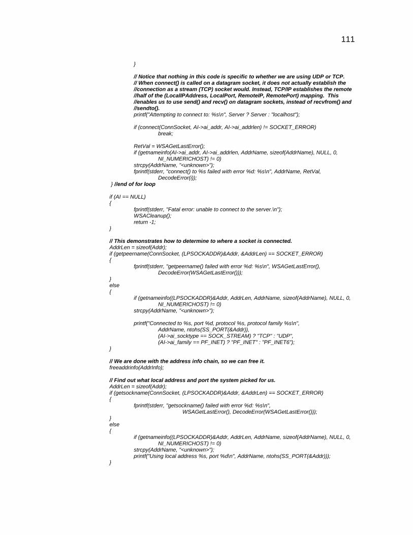
APPENDIX B: SOURCE CODE ...............................................................109

B.1 IPv4 and IPv6 in Windows 2000.................................109

B.2 IPv4 and IPv6 in Solaris 8.0 .......................................112

B.3 Microsecond Timer Granularity in Windows

2000.............................................................................115

APPENDIX C: ROUTER CONFIGURATIONS..........................................117

BIBLIOGRAPHY...............................................................................................119

viii

ix

ABSTRACT.......................................................................................................125

AUTOBIOGRAPHICAL STATEMENT..............................................................127

ix

x

LIST OF TABLES

TABLE PAGE

Table 1: Packet breakdown and overhead incurred by header information;

please refer to Equation 1 for obtaining the information above ........16

Table 2: Differences between IPv4 and IPv6 protocol [22] ......................26

Table 3: Differences between IPv4 and IPv6 headers [22] ......................27

Table 4: P2P Test-bed: TCP and UDP socket creation time and TCP

connection time in microseconds for both IPv4 and IPv6 running

Windows 2000 and Solaris 8.0 .........................................................60

Table 5: P2P Test-bed: the number of TCP connections per second for

IPv4 and IPv6 running Windows 2000 and Solaris 8.0 .....................61

Table 6: P2P Test-bed: frame rates and transfer rates for the video

client/server application for both IPv4 and IPv6 running Windows

2000..................................................................................................62

Table 7: IBM-Ericsson Test-bed: TCP and UDP socket creation time and

TCP connection time in microseconds for both IPv4 and IPv6 running

Windows 2000 and Solaris 8.0 .........................................................73

x

xi

Table 8: IBM-Ericsson Test-bed: The number of TCP connections per

second for IPv4 and IPv6 running Windows 2000 and Solaris 8.0 ...74

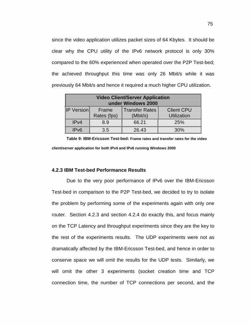
Table 9: IBM-Ericsson Test-bed: Frame rates and transfer rates for the

video client/server application for both IPv4 and IPv6 running

Windows 2000 ..................................................................................75

Table 10: IBM-Ericsson Test-bed: TCP and UDP socket creation time and

TCP connection time in microseconds for both IPv4, IPv6, and the

transition mechanisms running Windows 2000...............................100

Table 11: IBM-Ericsson Test-bed: The number of TCP connections per

second over IPv4, IPv6, and the transition mechanisms running

Windows 2000 ................................................................................101

Table 12: IBM-Ericsson Test-bed: Frame rates and transfer rates for the

video client/server application for IPv4, IPv6 and the transition

mechanisms running Windows 2000 ..............................................102

xi

xii

LIST OF FIGURES

FIGURE PAGE

Figure 1: OSI Reference Model ...............................................................10

Figure 2: TCP/IP Reference Model; on the left the various levels are

identified while on the right examples of functionality/protocol at each

respective layer.................................................................................11

Figure 3: IPv4 Packet as depicted by the Microsoft Network Monitor ......17

Figure 4: IPv6 Packet as depicted by the Microsoft Network Monitor ......18

Figure 5: Host-to-Host tunneling; packet traversal across a network .......31

Figure 6: IPv6 packet encapsulated in an IPv4 packet depicted by the

Microsoft Network Monitor ................................................................32

Figure 7: Router-to-Router Tunneling; packet traversal across a network

..........................................................................................................34

Figure 8: Test-bed architecture named IBM-Ericsson; two routers are

depicted, an IBM 2216 Nways Multiaccess Connector Model 400 and

an Ericsson AXI 462 .........................................................................36

Figure 9: Test-bed architecture named Ericsson; one router configuration

is depicted using the Ericsson AXI 462.............................................39

xii

xiii

Figure 10: Test-bed architecture named IBM; one router configuration is

depicted using the IBM 2216 Nways Multiaccess Connector Model

400....................................................................................................40

Figure 11: Test-bed architecture named P2P for point-to-point; PCs are

directly connected to each other via a twisted pair Ethernet cable ...40

Figure 12: P2P Test-bed: TCP throughput results for IPv4 & IPv6 over

Windows 2000 & Solaris 8.0 with packet size ranging from 64 bytes

to 64 Kbytes ......................................................................................50



to 1408 bytes ....................................................................................51

Figure 14: P2P Test-bed: UDP throughput results for IPv4 & IPv6 over


to 64 Kbytes ......................................................................................52



to 1408 bytes ....................................................................................53

Figure 16: P2P Test-bed: CPU Utilization results for the throughput

experiments in IPv4 and IPv6 running TCP and UDP over Windows

2000 with packet size ranging from 64 bytes to 64 Kbytes ...............54

xiii

xiv

Figure 17: P2P Test-bed: TCP latency results for IPv4 & IPv6 over


to 64 Kbytes ......................................................................................55

Figure 18: P2P Test-bed: TCP latency results for IPv4 & IPv6 over


to 1408 bytes ....................................................................................56

Figure 19: P2P Test-bed: UDP latency results for IPv4 & IPv6 over


to 64 Kbytes ......................................................................................57

Figure 20: P2P Test-bed: UDP latency results for IPv4 & IPv6 over


to 1408 bytes ....................................................................................58

Figure 21: P2P Test-bed: CPU Utilization results for the latency



Figure 22: IBM-Ericsson Test-bed: TCP throughput results for IPv4 & IPv6

over Windows 2000 & Solaris 8.0 with packet size ranging from 64

bytes to 64 Kbytes ............................................................................63



bytes to 1408 bytes...........................................................................64

xiv

xv

Figure 24: IBM-Ericsson Test-bed: UDP throughput results for IPv4 & IPv6


bytes to 64 Kbytes ............................................................................65



bytes to 1408 bytes...........................................................................66

Figure 26: IBM-Ericsson Test-bed: CPU Utilization results for the

throughput experiments in IPv4 and IPv6 running TCP and UDP over

Windows 2000 with packet size ranging from 64 bytes to 64 Kbytes67

Figure 27: IBM-Ericsson Test-bed: TCP latency results for IPv4 & IPv6


bytes to 64 Kbytes ............................................................................68

Figure 28: IBM-Ericsson Test-bed: TCP latency results for IPv4 & IPv6


bytes to 1408 bytes...........................................................................69

Figure 29: IBM-Ericsson Test-bed: UDP latency results for IPv4 & IPv6


bytes to 64 Kbytes ............................................................................70

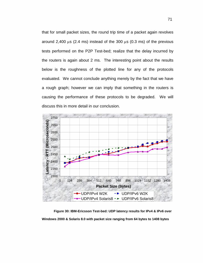
Figure 30: IBM-Ericsson Test-bed: UDP latency results for IPv4 & IPv6


bytes to 1408 bytes...........................................................................71

xv

xvi

Figure 31: IBM-Ericsson Test-bed: CPU Utilization results for the latency



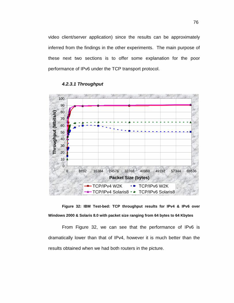
Figure 32: IBM Test-bed: TCP throughput results for IPv4 & IPv6 over


to 64 Kbytes ......................................................................................76



to 1408 bytes ....................................................................................77

Figure 34: IBM Test-bed: TCP latency results for IPv4 & IPv6 over


to 64 Kbytes ......................................................................................78

Figure 35: IBM Test-bed: TCP latency results for IPv4 & IPv6 over


to 1408 bytes ....................................................................................79

Figure 36: Ericsson Test-bed: TCP throughput results for IPv4 & IPv6 over


to 64 Kbytes ......................................................................................80



to 1408 bytes ....................................................................................81

xvi

xvii

Figure 38: Ericsson Test-bed: TCP latency results for IPv4 & IPv6 over


to 64 Kbytes ......................................................................................82



to 1408 bytes ....................................................................................83

Figure 40: IBM-Ericsson Test-bed: TCP throughput results for IPv4, IPv6,

and IPv4-IPv6 transition mechanisms under Windows 2000 with

packet size ranging from 64 bytes to 64 Kbytes ...............................88



packet size ranging from 64 bytes to 1408 bytes..............................89

Figure 42: IBM-Ericsson Test-bed: UDP throughput results for IPv4, IPv6,


packet size ranging from 64 bytes to 64 Kbytes ...............................90



packet size ranging from 64 bytes to 1408 bytes..............................91

Figure 44: IBM-Ericsson Test-bed: CPU utilization for TCP throughput

results for IPv4, IPv6, and IPv4-IPv6 transition mechanisms under


xvii

xviii

Figure 45: IBM-Ericsson Test-bed: CPU utilization for UDP throughput

results for IPv4, IPv6, and IPv4-IPv6 transition mechanisms under


Figure 46: IBM-Ericsson Test-bed: TCP latency results for IPv4, IPv6, and

IPv4-IPv6 transition mechanisms under Windows 2000 with packet

size ranging from 64 bytes to 64 Kbytes ...........................................94



size ranging from 64 bytes to 1408 bytes .........................................95

Figure 48: IBM-Ericsson Test-bed: UDP latency results for IPv4, IPv6, and


size ranging from 64 bytes to 64 Kbytes ...........................................96



size ranging from 64 bytes to 1408 bytes .........................................97

Figure 50: IBM-Ericsson Test-bed: CPU utilization for TCP latency results

for IPv4, IPv6, and IPv4-IPv6 transition mechanisms under Windows


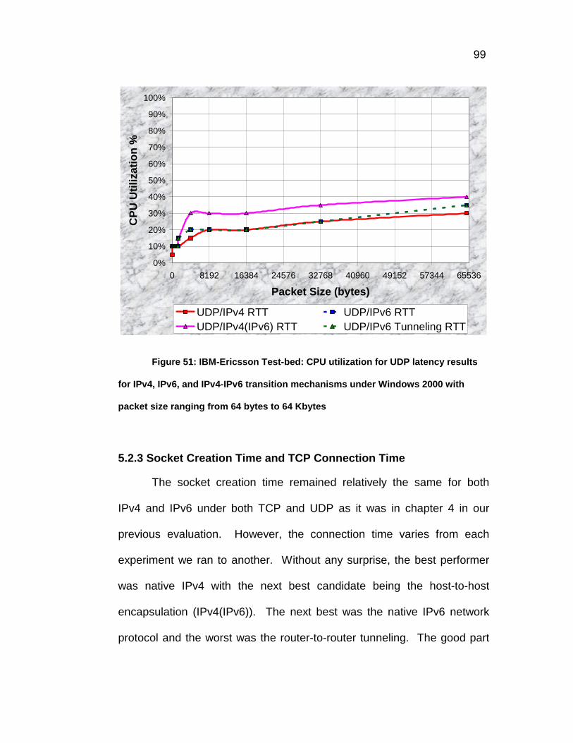
Figure 51: IBM-Ericsson Test-bed: CPU utilization for UDP latency results

for IPv4, IPv6, and IPv4-IPv6 transition mechanisms under Windows


Figure 52: Windows 2000 IPv4/IPv6 source code .................................112

xviii

xix

Figure 53: Solaris 8.0 IPv4/IPv6 source code ........................................114

Figure 54: MyTimeGetTime() – Retrieves microseconds since boot-up

under Windows 2000 ......................................................................116

Figure 55: Ericsson AXI 462 router configuration commands ................118

xix

1

CHAPTER 1

INTRODUCTION

It is a well known fact today’s networks, mainly the Internet, has

surpassed IPv4’s (Internet Protocol Version 4) [1, 9] capabilities. In the

simplest definition of IP, the Internet Protocol is the heart of most of the

modern networks. Without IP, the Internet as we know it would not have

existed and therefore the fundamentals that made the original IP possible

need to be preserved, enhanced, and redeployed in order for the Internet

to survive. The shortcomings of IPv4 were seen well in advance, and

therefore work started almost a decade ago. Its successor will be IPv6

(Internet Protocol Version 6) [2, 8, 9], and according to most experts, over

the next five to ten years, IPv6 will be slowly integrated into the existing

IPv4 infrastructure. [9]

IPv6 hopes to solve numerous problems that IPv4 has been

plagued by over the past two decades, however it will accomplish it at a

performance overhead. This performance loss is only using traditional

data transfers in which many of IPv6’s features supporting QoS (Quality of

Service) traffic are not used. Although the QoS support features of IPv6

will be briefly discussed, it is a topic in itself which ultimately is outside the

scope of our work for this thesis.

We tried to keep the experimentation as simple as possible to have

2

a good base of comparisons before we attempt to repeat similar test using

more features. Our experiments were conducted over an unloaded

network using two routers and various workstations. Most of the

experiments were conducted with the workstations running both Windows

2000 and Solaris 8.0, however some were only performed on Windows

2000.

Chapter 2 covers some background information about IPv4 and

IPv6 in general, and some of the fundamental differences between the

two network protocols; it also delves into the various transition

mechanisms that are available when upgrading from IPv4 to IPv6.

Chapter 3 explains the various test-bed configurations and each one’s

respective important characteristics. Chapter 4 offers the performance

metrics as well as the experimental results and explanations of IPv4

versus IPv6. Chapter 5 offers a similar evaluation as chapter 4, except

that it focuses on the transition mechanisms. Chapter 6 will cover future

work and the conclusions drawn from our evaluation. Chapter 7 is

Appendix A which is mainly a glossary of important terms with definitions.

Finally, chapter 8 is Appnedix B which includes sample source code which

clearly outlines the source code that is needed to implement both IPv4

and IPv6 ready applications.

Our goal was to perform an unbiased empirical performance

evaluation between the two protocol stacks (IPv4 and IPv6), and at the

3

same time, compare two different implementations (Windows 2000 and

Solaris 8.0) on identical hardware and under identical settings. Through

our experiments, we hope to emphasize the benefits and drawbacks to

either of these network protocol stacks.

4

CHAPTER 2

BACKGROUND INFORMATION

This chapter’s main goals are to familiarize the reader with the

subject at hand. First some related work is discussed, in terms of what

work has been done in the research community that is most similar to our

work. With no surprise, we found nothing that was even close to the wide

range of performance metrics and comparing two different

implementations, two different network protocols, and two different

transport protocols. By covering some of other people’s work, our own

motivation will prevail in terms of why we pursued the avenue we did and

what is the value of our findings. An in-depth description of IPv4, IPv6,

and the transition mechanisms are presented. In order to better

understand the Internet Protocol, layering principles are first described in

section 2.2.

2.1 Related Work

Our work was driven by the fact that there was no good comparison

between IPv4 and IPv6 that was conducted in a scientific method and

tried to depict the real world scenario in both IPv4 and IPv6 protocol

stacks would have to traverse routers to reach their ultimate destination.

Even if some of the experiments in the research community used routers,

5

they were always software routers built from conventional PCs and had

installed FreeBSD in order to handle the necessary routing.

Most of the industry wide routers implement most of their

functionality in hardware and therefore are much more efficient than a

software router approach which was taken by most researchers.

Obviously there is a very good explanation to why nobody has tested

IPv6’s performance using real routers: hardware based routers supporting

dual stack IPv4/IPv6 are rare and expensive. As an example, the two

routers which we used for our experiments cost a total of US $60,000,

which is a price tag out of reach for most research laboratories.

Furthermore, we also tested two different implementations, namely

Windows 2000 and Solaris 8.0, side by side, throughout all of our

experiments; we covered both TCP and UDP transport protocols. Our

metrics included throughput, latency, CPU utilization, socket creation time,

TCP connection time, the number of TCP connections per second, and

the performance of a video application designed by our lab. This is in

essence our contribution that nobody else has been able to accomplish:

an unbiased empirical evaluation of two different implementations of IPv6

covering all the basic performance metrics and transport protocols under

a realistic test-bed configuration.

The next few paragraphs will cover some of the work that had

similar goals as our own; however they stopped short of accomplishing

6

the task at hand when compared to our results. In [34], the first attempt at

developing an IPv6 protocol stack for Windows NT is shown. The work

presented is very old (early 1998) and offers some performance

evaluation of a very specific instance of the wide range of tests we

performed. I am sure they choose the best case scenario in order to

show that their IPv6 implementation was almost as good as its IPv4

counterpart. They never mentioned what packet size they used for their

transmission and they only utilized the TCP transport protocol. They also

had no router and hence only connected the two PCs with a direct cable

link. Most likely, there were no routers supporting IPv6 back in early

1998. They also did not do many tests such as latency, CPU utilization,

socket creation time, etc.

In [36], the author evaluated the MSR IPv6 BETA protocol stack for

Windows NT 4.0. The author evaluated the performance of MSR IPv6

protocol stack by measuring and analyzing its network latency,

throughput, and processing overheads. Their test-bed consisted of two

Pentium machines with 100Mbps fast Ethernet connected via an

unloaded switch. The work presented seemed interesting and contained

only a small part of our work. First of all, it only evaluated IPv6 and did

not compare it with IPv4. Secondly, they only evaluated the Windows NT

implementation and did not compare it with any other implementations.

Notice that there were no routers involved in their experimentation and

7

only connected their hosts with a switch. Obviously the findings they

made are nearly obsolete since IPv6 and computing hardware evolved so

much since 1999. For example the MSR IPv6 protocol stack has been

replaced by the Windows 2000 IPv6 Preview Protocol Stack. Regardless,

their work showed very interesting initial results on IPv6.

In [35], the authors evaluate the performance of data transmission

over IPv4 and IPv6 suing various security protocols. The authors choose

a particular application, namely digital video (DV) transmission in order to

execute their experiments. They utilized end hosts with FreeBSD 2.2.8

and KAME IPv6 protocol stack and a router implemented in a PC platform

also running FreeBSD 2.2.8 and KAME IPv6 protocol stack. The criticism

of this work lies in the fact that the routers utilized obviously did not

support most of the router functions in the hardware and therefore the

depicted performance is lower than the performance in a real world

scenario in which actual hardware routers would be utilized. One of the

other criticisms is that they only covered small sample of the test we

performed. They utilized two different buffer sizes (57344 bytes and

32769 bytes), which makes no sense; it is a known fact that when

performing experiments of this nature, the buffer size is kept constant

throughout all the experiments. They claim that the MTU size they used

was either 1024 or 4096 bytes, however IP routers do not support MTU

sizes above 1514 bytes. They might have had the functionality to change

8

the MTU size beyond the maximum due to the software router

implementation they were using. Obviously such a large MTU size might

yield falsely higher than usual results. The only place where they

mentioned the packet size, they specified 32 KB packets, but they called it

the socket size. As an overall evaluation, the depicted results are

interesting, but not complete in the sense of depicting real world

performance.

In both [37, 33], the authors presented an evaluation of IPv6

compared to IPv4 using the dual stack implementation of KAME over

FreeBSD OS using the ping utility and a FTP application; their metrics

were latency and throughput. The major criticism of the work presented in

[33, 37] is that the experiments were not done in a scientific manner.

They used a ported FTP application to find out the throughput rates of the

IPv6 protocol; they used the ping utility to find the latency. In [33], they

had no router, but rather connected the two end hosts via a hub. In [37],

they had a router which was a conventional PC using the FreeBSD router

software. They obviously could not control any critical parameters, such

as buffer size, packet size, and of course they could not perform any UDP

tests due to the nature of FTP.

After reading all the related work performed in the research

community, it should be clear that there was a need for the evaluation we

performed in our research endeavors.

9

2.2 Layering Principles

Layering is one of the major reasons network architectures have

been so successful. One great success story is the Internet, which shows

how robust and scalable it has been despite the initial design goals which

did not foresee the exponential growth that it indured.

Layering helps break complex problems into smaller more

manageable pieces. It helps reduce design complexity and it simplifies

the design and testing protocols. Sender and receiver software can be

tested, designed and implemented independently. Layering prevents

changes in software from propagation to other layers. It allows designers

to construct protocol suites and allows ease of change regarding an

implementation of a service. Some of its drawbacks include some

performance loss, time delay, and perhaps having more than 1 copy of

data at any given moment. Obviously, these drawbacks are quickly

overshadowed by all the advantages of a layered approach to designing

protocols.

The basic definition of layering is that the layer N software on the

receiving machine should receive the exact message sent by the layer N

software at the sender machine. It should satisfy whatever transformation

was applied to the packet should be completely reversible at the receiving

side.

10

2.2.1 OSI Reference Model

The OSI model is not a network architecture because it does not

specify exact services and protocols. It is designed for open system

interconnection. Each layer should represent a well defined function and

a new layer is needed when a new level of abstraction is required. The

layers should be chosen in order to minimizing flow of information across

layers. And last of all, each layer should be chosen towards standardizing

protocols.

I will be concentrating my efforts on three layers, namely the

network layer, the transport layer, and the application layer. Figure 1

depicts the OSI reference model and its 7 layers. Since we will mainly

concentrate on IPv4 and IPv6, it is relevant to discuss the TCP/IP

reference model, in which we will describe some of the necessary layers

in more detail.

The OSI model is composed of 7 layers:

Figure 1: OSI Reference Model

Layer 1: Application layer Layer 2: Presentation layer Layer 3: Session layer Layer 4: Transport layer Layer 5: Network layer Layer 6: Data link layer Layer 7: Physical layer

11

2.2.2 TCP/IP Reference Model

The TCP/IP model is composed of 4 layers:

Figure 2: TCP/IP Reference Model; on the left the various levels are

identified while on the right examples of functionality/protocol at each respective

layer

The Internet layer, known as the network layer in the OSI model,

allows heterogeneous networks to be connected. It provides congestion

control, it establishes, maintains, and tears down connections, and most

important of all, it determines the route of packets transmitted. Both the

IP protocol versions, IPv4 and IPv6, are found in the network layer. Due

to the diverse functionality of this layer, it should be obvious that it is very

important that the services maintained by the network layer are the key to

the entire protocol stack’s triumph.

The transport layer provides reliable, transparent data transfers

between senders and receivers. It provides error recovery mechanism

12

and flow control in order to throttle the sending rates. It also fragments

data into smaller pieces, and passes them down to the network layer.

Both TCP and UDP are found in the transport layer.

The application layer has many protocols used in conjunction with

the application. TELNET, FTP, and DNS are only a few that are among

the protocols that applications can use.

2.3 IPv4 and IPv6 Architecture

Internet Protocol was first developed in the early 1980s. Its intent

was to interconnect few nodes and was never expected to grow to the

size of the Internet has become today. IPv4 was initially designed for

best-effort service and only scaled to today’s Internet size because of its

state-less design. One of the few things that the creators of the Internet

Protocol never envisioned was the exhaustion of a 32 bit address space.

In the early 1990s, it became pretty evident that if the Internet will

continue to grow at the exponential rate of doubling every eighteen

months, the IPv4 address space would be depleted by the turn of the

millennium. Some temporary solutions were offered, such as NAT

(Network Address Translator) [4] or CIDR (Classless InterDomain

Routing) [9], however work began on a new Internet Protocol, which was

first called IPnG from Internet Protocol Next Generation, but later became

known as IPv6, Internet Protocol version 6 (IPv6). IPv6 is the main focus

13

of our work and hence this thesis.

The most evident reason for a new version of an IP was to

increase the address space; IPv6 was designed with a 128 bit address

schema, enough to label every molecule on the surface of the earth with a

unique address (7x1023 unique IP addresses per square meter) [9]. Even

in the most pessimistic scenario of inefficient allocation of addresses,

there would still be well over 1000 unique IP addresses per square meter

of the earth [5]. There were other reasons that were a bit more subtle,

such as better support for inelastic traffic and real time applications, and

without doubt will most likely drive the deployment of IPv6 just as hard as

the address space depletion problem. Twenty years ago, the only kind of

traffic that existed on the internet was elastic traffic, such as emails or file

transfers. Elastic traffic enjoys having high bandwidth and low latency,

however if the network can only deliver a small percentage of its capacity,

than the transmission will still deliver the data just as good, but just at a

later time. On the other hand, inelastic traffic has much more stringent

restrictions in which bad network performance can render the data

useless. In the past five years, multimedia applications have emerged

and have mostly dominated the Internet’s growth and demand for more

bandwidth and processing power. IPv6 was designed for both elastic and

inelastic traffic in its vision scope. That does not mean that IPv6 is not a

best effort service anymore, but merely that it has the potential to

14

interoperate much easier with Quality of Service (QoS) architectures such

as RSVP [15], Integrated Services (Intserv) [16,17], and Differentiated

Services (Diffserv) [18] in order to make end-to-end QoS over IP-based

networks a reality. These features of IPv6 are outside the context of this

paper, so please refer to Chapter 5 in regards to future work.

Some of the differences between IPv4 and IPv6 features are

outlined in the next few statements. Keep in mind that most of the

improvements on IPv6 were done with three things in mind: scalability,

security, and support for multimedia transmissions. First of all, the

address space is increased from 32 bits to 128 bits. Obviously, this

increase in address space means more capacity for nodes, but it also

enlarges the header overhead and the routing tables’ size. Unlike IPv4,

IPSec support has become a requirement in the IPv6 header. This was a

much needed improvement to at least offer basic security features.

Payload identification for QoS handling by routers is now supported by the

flow label field. This was introduced primarily because of the earlier

statements about multimedia applications that require more stringent

guarantees of data delivery. Fragmentation support has been moved

from both routers and sending hosts to just sending hosts. This is an

important fact due to the amount of work that the routers have been

alleviated by, and therefore it improves scalability. The IPv6 header does

not include a checksum and has no options included in the header, but

15

rather introduces extension headers. This allows faster processing at the

routers by performing the checksum less often and analyzing only the

header information needed. Finally, IPv6 requires no manual

configuration or DHCP, which will become more and more important as

the number of nodes increases. Overall, IPv6 was carefully thought out

and was designed with future applications in mind. [9]

Theoretically, taking a close look at the brake-down of the various

headers in both IPv4 and IPv6, it is evident that the overhead incurred is

minimal between IPv4 and IPv6. As a quick overview of Table 1 found

below, the primary difference between IPv4 and IPv6 is that IPv4 has a 20

byte header while IPv6 has a 40 byte header. Although the address

space in IPv6 is four times the size of its counterpart, IPv6 has decreased

the number of required fields and made them optional as extension

headers. Let’s take the IPv4 UDP packet as an example to better

understand Table 1. The total Ethernet MTU (Maximum Transfer Unit) is

1514 bytes, from which 14 bytes are the Ethernet header, 20 bytes are

the IP header, and 8 bytes are the UDP header. The payload for a UDP

packet in IPv4 is 1472 bytes, and is computed by Equation 1:

MTU = Payload + TLH + NLH + DLLH

Equation 1: MTU calculation; the formula used in deriving Table 1; payload

is the application layer data size; TLH is the transport layer (TCP/UDP) header size;

NLH is the network layer (IP) header size; DLLH is the data link (Ethernet) layer

16

header size; MTU is the total Ethernet MTU size that is transmitted on the physical

medium.

IPv4 TCP

IPv6 TCP

IPv4 UDP

IPv6 UDP

TCP/UDP Payload 1460 1440 1472 1452 TCP/UDP Header 20 20 8 8

IP Payload 1480 1460 1480 1460 IP Header 20 40 20 40

Ethernet Header 14 14 14 14 Total Ethernet MTU 1514 1514 1514 1514

Overhead % 3.7% 5.14% 2.85% 4.27%

Table 1: Packet breakdown and overhead incurred by header information;

please refer to Equation 1 for obtaining the information above

The difference between IPv4 and IPv6 would most obviously be the

IP header, which instead of being 20 bytes, would now be 40 bytes. The

overhead that is incurred by having header information can be figured out

by taking the total Ethernet MTU and dividing by the TCP or UDP payload.

For example, the difference between IPv4 UDP and IPv6 UDP is a mere

1.42 %, while for TCP it is almost the same at 1.44 %.

In theory, the performance overhead between these two protocols

is so minimal that the benefits of IPv6 should quickly overshadow the

negatives. In Chapter 4 and 5, I will discuss the performance evaluation

in reality between IPv4 and IPv6, which proved to be quite a bit larger than

the theoretical difference.

In order to better visualize the layering principles, we captured a

screen shot of Microsoft Network Monitor as it displays a packet and all its

17

header information and placed in Figure 3 and Figure 4. Figure 3 displays

a ping echo (ICMP) message and its header information. Notice that the

IP version is 4 and the IP header length is 20 bytes. Notice also the

source and destination addresses, as they are all part of the packet

header information.

Figure 3: IPv4 Packet as depicted by the Microsoft Network Monitor

Figure 4 will show a similar screen shot, but this time presenting an

IPv6 packet. Figure 4 displays a ping echo (ICMP) message and its

header information for an IPv6 packet. Notice that the IP version is 6 and

the IP header length is 40 bytes. Notice also the IPv6 128 bit source and

destination addresses, as they are all part of the packet header

18

information. Some new fields can also be seen, such as priority, flow

label, and next header. We will discuss these in more detail later.

Figure 4: IPv6 Packet as depicted by the Microsoft Network Monitor

2.3.1 IPv4 Specifications

Internet Protocol version 4 is the current version of IP, which was

finally revised in 1981. It has a 32 bit address looking like

255.255.255.255, and it supports up to 4,294,967,296 (4.3x109)

addresses. The IPv6 header is a streamlined version of the IPv4 header.

It eliminates fields that are unneeded or rarely used and adds fields that

provide better support for real-time traffic. An overview of the IPv4 header

is helpful in understanding the IPv6 header.

19

The “Version” field indicates the version of IP and is set to 4 in the

case of IPv4; the size of this field is 4 bits.

The “Internet Header Length” field indicates the number of 4-byte

blocks in the IP header. The size of this field is 4 bits. The minimum IP

header size is 20 bytes, and therefore the smallest value of the Internet

Header Length field is 5. IP options can extend the minimum IP header

size in increments of 4 bytes. If an IP option does not use all 4 bytes of

the IP option field, the remaining bytes are padded with 0’s, making the

entire IP header an integral number of 32-bits (4 bytes). With a maximum

value of 0xF, the maximum size of the IP header including options is 60

bytes (15*4).

The “Type of Service” field indicates the desired service expected

by this packet for delivery through routers across the IP internetwork. The

size of this field is 8 bits, which contain bits for precedence, delay,

throughput, and reliability characteristics. Unfortunately, this field was not

widely utilized, and only recently with the coming of RSVP did it see much

activity. For example, RSVP uses the type of service field in order to

setup flow labels.

The “Total Length” field indicates the total length of the IP packet

(IP header + IP payload) and does not include link layer framing. The size

of this field is 16 bits, which can indicate an IP packet that is up to 65,535

bytes long.

20

The “Identification” field identifies the specific IP packet. The size of

this field is 16 bits. The Identification field is selected by the originating

source of the IP packet. If the IP packet is fragmented, all of the fragments

retain the Identification field value so that the destination node can group

the fragments for reassembly.

The “Flags” field identifies flags for the fragmentation process. The

size of this field is 3 bits, however, only 2 bits are defined for current use.

There are currently two flags: one indicates whether the IP packet might

be fragmented, while the other indicates whether more fragments follow

the current fragment.

The “Fragment Offset” field indicates the position of the fragment

relative to the original IP payload; the size of this field is 13 bits.

The “Time-to-Live” (TTL) field indicates the maximum number of

links on which an IP packet can travel before being discarded. The size of

this field is 8 bits. The TTL field was originally used as a time count with

which an IP router determined the length of time required (in seconds) to

forward the IP packet, decrementing the TTL accordingly. Modern routers

almost always forward an IP packet in less than a second and are

required by RFC 791 [1] to decrement the TTL by at least one. Therefore,

the TTL becomes a maximum link count with the value set by the sending

node. When the TTL equals 0, the packet is discarded and an ICMP Time

Expired message is sent to the source IP address.

21

The “Protocol” field identifies the upper layer protocol; the size of

this field is 8 bits. For example, TCP uses a protocol value of 6, UDP

uses a protocol value of 17, and ICMP uses a protocol value of 1. The

Protocol field is used to demultiplex an IP packet to the upper layer

protocol.

The “Header Checksum” field provides a checksum on the IP

header only. The size of this field is 16 bits. The IP payload is not included

in the checksum calculation as the IP payload and usually contains its

own checksum. Each IP node that receives IP packets verifies the IP

Header Checksum and silently discards the IP packet if checksum

verification fails. When a router forwards an IP packet, it must decrement

the TTL. Therefore, the Header Checksum is recomputed at each hop

between source and destination.

The “Source Address” field stores the IP address of the originating

host; the size of this field is 32 bits.

The “Destination Address” field stores the IP address of the

destination host; the size of this field is 32 bits.

The “Options” field stores one or more IP options. The size of this

field is a multiple of 32 bits. If the IP options do not use all 32 bits, padding

options must be added so that the IP header is an integral number of 4-

byte blocks that is indicated by the Internet Header Length field.

22

2.3.2 IPv6 Specifications

Internet Protocol version 6 is designed as an evolutionary upgrade

to the Internet Protocol (IPv4) and will, in fact, coexist with the older IPv4

for some time. IPv6 is designed to allow the Internet to grow steadily, both

in terms of the number of hosts connected and the total amount of data

traffic transmitted; it will have a 128 bit address looking like

1234:5678:90AB:CDEF:FFFF:FFFF:FFFF:FFFF, and it will support up to

340,282,366,920,938,463,463,374,607,431,768,211,456 (3.4x1038)

unique addresses.

The IPv6 header is always present and is a fixed size of 40 bytes.

The fields in the IPv6 header are described briefly below.

The “Version” field is used to indicate the version of IP and is set to

6 in the case of IPv6; the field size is 4 bits.

The “Traffic Class” field indicates the class or priority of the IPv6

packet. The size of this field is 8 bits. The Traffic Class field provides

similar functionality to the IPv4 Type of Service field. In RFC 2460, the

values of the Traffic Class field are not defined. However, an IPv6

implementation is required to provide a means for an application layer

protocol to specify the value of the Traffic Class field for experimentation.

The “Flow Label” field indicates that this packet belongs to a

specific sequence of packets between a source and destination, requiring

23

special handling by intermediate IPv6 routers. The size of this field is 20

bits. The Flow Label is used for non-default quality of service connections,

such as those needed by real-time data (voice and video). For default

router handling, the Flow Label is set to 0. There can be multiple flows

between a source and destination, as distinguished by separate non-zero

Flow Labels.

The “Payload Length” field indicates the length of the IP payload.

The size of this field is 16 bits. The Payload Length field includes the

extension headers and the upper layer PDU. With 16 bits, an IPv6

payload of up to 65,535 bytes can be indicated. For payload lengths

greater than 65,535 bytes, the Payload Length field is set to 0 and the

Jumbo Payload option is used in the Hop-by-Hop Options extension

header.

The “Next Header” field indicates either the first extension header

(if present) or the protocol in the upper layer PDU (such as TCP, UDP, or

ICMPv6, etc). The size of this field is 8 bits. When indicating an upper

layer protocol above the Internet layer, the same values used in the IPv4

Protocol field are used here.

The “Extension Header” field is utilized for additional functionality

that might be needed, such as jumbo packet sizes, security, etc. Zero or

more extension headers can be present and are of varying lengths. A

Next Header field in the IPv6 header indicates the next extension header.

24

Within each extension header is another Next Header field that indicates

the next extension header. The last extension header indicates the upper

layer protocol (such as TCP, UDP, or ICMPv6) contained within the upper

layer protocol data unit. The IPv6 header and extension headers replace

the existing IPv4 IP header with options. The new extension header

format allows IPv6 to be augmented to support future needs and

capabilities. Unlike options in the IPv4 header, IPv6 extension headers

have no maximum size and can expand to accommodate all the extension

data needed for IPv6 communication.

The “Hop Limit” field indicates the maximum number of links over

which the IPv6 packet can travel before being discarded. The size of this

field is 8 bits. The Hop Limit is similar to the IPv4 TTL field except that

there is no historical relation to the amount of time (in seconds) that the

packet is queued at the router. When the Hop Limit equals 0, the packet is

discarded and an ICMP Time Expired message is sent to the source

address.

The “Source Address” field stores the IPv6 address of the

originating host; the size of this field is 128 bits.

The “Destination Address” field stores the IPv6 address of the

destination host; the size of this field is 128 bits. In most cases the

Destination Address is set to the final destination address. However, if a

Routing extension header is present, the Destination Address might be set

25

to the next router interface in the source route list.

2.3.3 IPv4 vs. IPv6

Table 2 shows the highlights in the differences between IPv4 and

IPv6 protocols. There are many other differences; however, it depends on

what level of detail we wish to examine the matter. There have been

entire books written on the IPv6 protocol and all the differences down to

the minutest detail from the old IPv4 protocol. One such book is “IPv6

Networks” [22] by Marcus A. Goncalves; it offers an excellent in-depth

explanation of any material covered here in this chapter regarding IPv6

networks and much more.

An important aspect of the following information is that the facts

presented in Table 2 and Table 3 are all theoretical. These are all the

proposed changes that have been outline in the various Requests for

Comments (RFC) lead by IETF. The actual implementation of all the

features is still in the infancy stages of development and there still lacks

maturity, as will be presented in our experimental results. Most likely, by

the time that IPv6 will be deployed worldwide and will replace IPv4, all the

features stated below should be implemented. Most experts predict that

in the next five years, most of the Internet will have support for IPv6.

The left hand side of the table represents features of IPv4 while the

right hand side represents features of IPv6; they are interrelated and

26

depict how the particular feature of IPv4 was upgraded to support IPv6.

Definitions of the terminology or acronyms can be found in Appendix A.

IPv4 IPv6 Source and destination addresses are 32 bits (4 bytes) in length.

Source and destination addresses are 128 bits (16 bytes) in length.

IPSec support is optional. IPSec support is required. No identification of payload for QoS handling by routers is present within the IPv4 header.

Payload identification for QoS handling by routers is included in the IPv6 header using Flow Label field.

Fragmentation is supported at both routers and the sending host.

Fragmentation is only supported at the sending host.

Header includes a checksum. Must be computed at every intervening node on a per packet basis.

Header does not include a checksum. It relies on other layers to find erroneous packets.

Header includes options. Potential inefficient use of header bits.

All optional data is moved to IPv6 extension headers.

Address Resolution Protocol (ARP) broadcast ARP Request to resolve an IPv4 address to the link layer.

ARP Request frames are replaced with multicast Neighbor Solicitation messages.

Internet Group Management Protocol (IGMP) is used to manage local subnet group membership.

IGMP is replaced with Multicast Listener Discovery (MLD) messages.

ICMP Router Discovery is used to determine the IPv4 address of the best default gateway.

ICMPv4 Router Discovery is replaced with ICMPv6 Router Solicitation and Router Advertisement.

Broadcast addresses are used to send traffic to all nodes on a subnet.

There are no IPv6 broadcast addresses; a link-local scope all-nodes multicast address is used.

Must be configured either manually or through DHCP.

Does not require manual configuration or DHCP.

Uses host address (A) resource records in the DNS to map host names to IPv4 addresses.

Uses host address (AAAA) resource records in the DNS to map host names to IPv6 addresses.

Pointer resource records (PTR) in IN-ADDR.ARPA DNS domain map IPv4 addresses to host names.

Uses pointer (PTR) resource records in the IP6.INT DNS domain to map IPv6 addresses to host names.

Table 2: Differences between IPv4 and IPv6 protocol [22]

27

Now that the main differences in the protocols are clear, Table 3

will describe the differences between the IPv4 and IPv6 header fields.

The left column names the header field while the right side describes the

change which IPv6 incurred from its IPv4 predecessor.

IPv4 Header Field IPv6 Header Field Version Same field but with different version numbers.

Internet Header Length

Removed in IPv6. IPv6 does not include a Header Length field because the IPv6 header is always a fixed size of 40 bytes. Each extension header is either a fixed size or indicates its own size.

Type of Service Replaced by the IPv6 Traffic Class field. Total Length Replaced by the IPv6 Payload Length field, which

only indicates the size of the payload. Identification Removed in IPv6. Fragmentation information is not

included in the IPv6 header. It is contained in a Fragment extension header.

Fragmentation Flags

Removed in IPv6. Fragmentation information is not included in the IPv6 header. It is contained in a Fragment extension header.

Fragment Offset Removed in IPv6. Fragmentation information is not included in the IPv6 header. It is contained in a Fragment extension header.

Time to Live Replaced by the IPv6 Hop Limit field. Protocol Replaced by the IPv6 Next Header field. Header

Checksum Removed in IPv6. In IPv6, bit-level error detection for the entire IPv6 packet is performed by the link layer.

Source Address The field is the same except that IPv6 addresses are 128 bits in length.

Destination Address

The field is the same except that IPv6 addresses are 128 bits in length.

Options Removed in IPv6. IPv4 options are replaced by IPv6 extension headers.

Table 3: Differences between IPv4 and IPv6 headers [22]

28

2.4 IPv4 to IPv6 Transition Mechanisms

As IPv6 is finally beginning to mature and IPv4 is approaching its

limits, it is evident that methods of upgrading the Internet from IPv4 to

IPv6 need to be found. One idea would be to turn off the entire Internet at

12AM, upgrade the network infrastructure (routers, protocol stacks, etc),

and turn the Internet back on at 6AM and hope everything works. This is

unrealistic due to the astronomical price and the high probability that it will

not work as well as the theoretical prediction. Hence, more gradual

transition methods have evolved, ones which are likely to happen over the

course of the next 10 years.

Some transition mechanisms are: Dual Stacks [3], DTI & Bump-

in-dual-stack, NAT Protocol Translator [27], Stateless IP/ ICMP Translator

(SIIT), Assignment of IPv4 Global Addresses to IPv6 Hosts (AIIH), Tunnel

Broker [28], 6-to-4 Mechanism [29], and IPv6 in IPv4 tunneling [30,31].

Dual Stacks are easiest to implement, however complexity

increases due to both infrastructures and the cost is higher due to a more

complex technology stack. NAT Protocol Translator has scaling and DNS

issues, and has single point of failure disadvantage. The Tunnel Broker

dynamically gains access to tunnel servers, but has authentication and

scaling issues. 6-to-4 mechanism creates dynamic stateless tunnels over

IPv4 infrastructure to connect 6-to-4 domains. IPv6 in IPv4 tunneling

29

allows existing infrastructure to be utilized via manually configured

tunnels.

We chose to pursue the IPv6 in IPv4 tunneling as a transition

mechanism because it would be the most cost effective and can

implement islands of IPv6 networks that can be connected over the

existing ocean of IPv4 networks, the existing infrastructure. With time, as

the islands grow, the ocean will diminish to a point that all the islands will

touch, at which point it is evident that native IPv6 networks will finally reign

and benefit 100% from its new features. There are two transition

mechanisms which we will discuss: host-to-host encapsulation and router-

to-router encapsulation, which is also know as tunneling. The router-to-

router tunneling is the more interesting of the two since entire LANs can

be upgraded to IPv6 while maintaining connectivity to the rest of the

Internet. Host-to-host encapsulation is also addressed mainly because of

its simplicity of implementation, and offers another method of making the

transition from IPv4 to IPv6 as smooth as possible.

Encapsulation of IPv6 packets within IPv4 packets, better known as

tunneling, is one of the easiest transition mechanisms by which two IPv6

hosts / networks can be connected with each other while running on

existing IPv4 networks through establishing some special routes called

tunnels. In this technique, IPv6 packets are encapsulated in IPv4 packets

and then are sent over IPv4 networks like ordinary IPv4 packets through

30

tunnels. At the end of tunnel these packets are de-capsulated to the

original IPv6 packets.

When encapsulating a datagram, the TTL in the inner IP header is

decremented by only one if the tunnel is being done as part of forwarding

the datagram; otherwise the inner header TTL is not changed during

encapsulation. If the resulting TTL in the inner IP header is zero, the

datagram is discarded and an ICMP Time Exceeded message is returned

to the sender. Therefore, an encapsulator will not encapsulate a

datagram with TTL=0. When encapsulating IPv6 packets in IPv4 packets,

only IPv4 routing properties will be utilized and hence the IPv6 packet will

loose any special IPv6 features until it is de-capsulated at the receiving

host/router. Another drawback is that it requires a hole in a firewall to

allow protocol 41 (IP in IP) passage.

If a tunnel falls entirely within a routing domain, it will be considered

as plain serial link by interior routing protocol such as RIP or OSPF. But if

it lies between two routing domains it needs exterior protocols such as

BGP. In case of congestion in the tunnel, an ICMP Source Quench

message will be issued in order to inform the previous node of the

congestion.

In different two different types of tunneling, only de/encapsulation

points are varied depending on the start and end of tunnels, however the

31

basic idea remains the same. Once again, the two tunneling mechanisms

are Host-Host Tunneling and Router-Router Tunneling.

2.4.1 Host-to-Host Encapsulation

In host-to-host tunneling method, encapsulation is done at the

source host and the de-capsulation is done at the destination host. So the

tunnel is created in between two hosts supporting both IPv4 and IPv6

stacks. Therefore, the encapsulated datagrams are sent through a native

IPv4 network that has no knowledge of the IPv6 network protocol.

Figure 5: Host-to-Host tunneling; packet traversal across a network

In Figure 5, it is clear that both hosts having dual stack encapsulate

the packets of IPv6 in IPv4 packets and transmit over the network as an

32

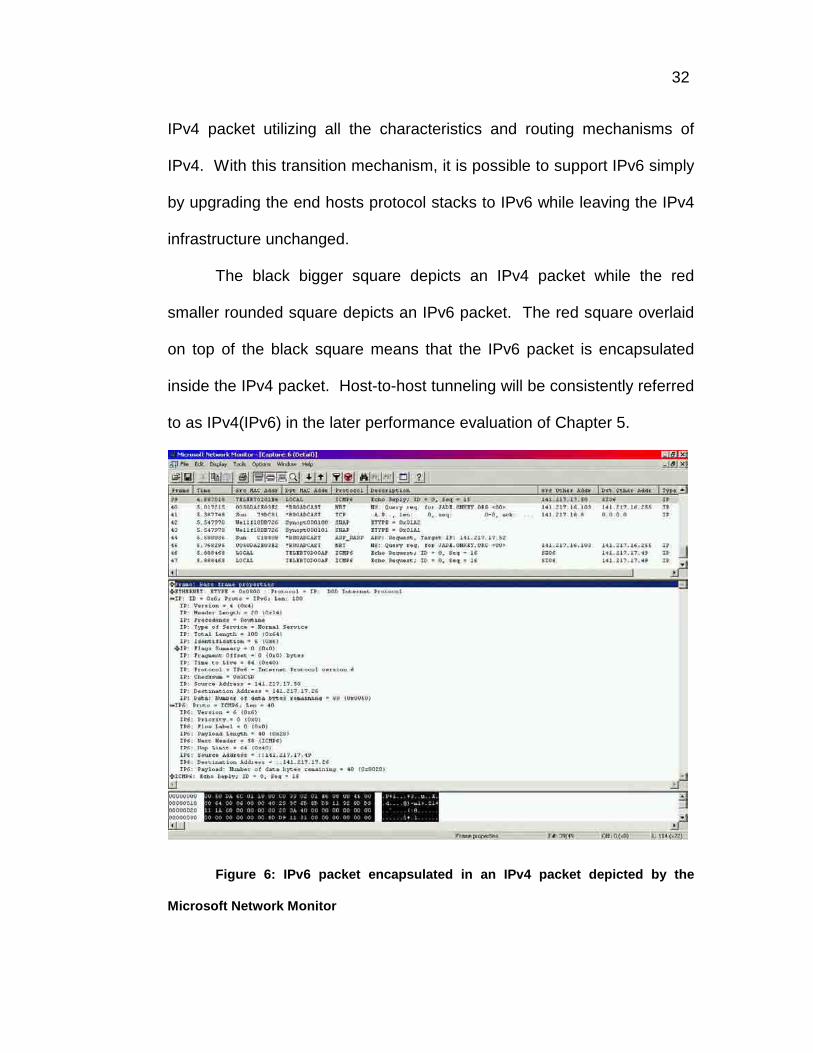
IPv4 packet utilizing all the characteristics and routing mechanisms of

IPv4. With this transition mechanism, it is possible to support IPv6 simply

by upgrading the end hosts protocol stacks to IPv6 while leaving the IPv4

infrastructure unchanged.

The black bigger square depicts an IPv4 packet while the red

smaller rounded square depicts an IPv6 packet. The red square overlaid

on top of the black square means that the IPv6 packet is encapsulated

inside the IPv4 packet. Host-to-host tunneling will be consistently referred

to as IPv4(IPv6) in the later performance evaluation of Chapter 5.

Figure 6: IPv6 packet encapsulated in an IPv4 packet depicted by the

Microsoft Network Monitor

33

Just as we displayed a picture of the IPv4 and IPv6 packet alone in

Figure 3 and Figure 4, we will show an IPv6 packet encapsulated in an

IPv4 packet in Figure 6 to illustrate to the reader how the hosts sees the

encapsulation. All the various header fields are clearly visible just as we

had described them in the earlier section.

2.4.2 Router-to-Router Tunneling

In router to router tunneling mechanism, encapsulation is done at

the edge router of the origination host and de-capsulation is done in the

same way at the edge router of the destination host. The tunnel is

created in between two edge routers supporting both IPv4 and IPv6

stacks. Therefore, the end hosts can support native IPv6 protocol stack

while the edge routers create the tunnels and handle the encapsulation

and de-capsulation in order to transmit the packets over the existing IPv4

infrastructure in between the two edge routers.

Figure 7 shows a tunnel established between two edge routers,

which supports both (IPv4 / IPv6) stacks. The IPv6 packets are forwarded

from host to edge routers while encapsulation takes place at the router

level; similarly at the other end, the reverse process takes place. In this

method, both edge routers need to support dual stacks and established a

tunnel prior to transmission.

34

Figure 7: Router-to-Router Tunneling; packet traversal across a network

35

CHAPTER 3

TEST-BED CONFIGURATION

Our test-bed consisted of two dual stack (IPv4/IPv6) routers: an

Ericsson AXI 462, and an IBM 2216 Nways Multiaccess Connector Model

400. Dual stack implementation specifications can be found in RFC 1933

[3]. We had two identical workstations that were connected directly to the

routers and were configured to be on separate networks. Each router

supported two separate networks each.

Both workstations were equipped with Intel Pentium III 500 MHz

processors, 256 megabytes of SDRAM PC100, two 30GB IBM 7200 RPM

IDE hard drive, and COM 10/100 PCI network adapters. The workstations

were loaded with both Windows 2000 Professional and Solaris 8.0 as a

dual boot configuration on two separate and identical hard drives.

Windows 2000 had the IPv4 stack as a standard protocol; however in

order to get IPv6 support, an add-on package was installed. There were

two choices, both written by Microsoft and they were both in Beta testing.

We chose the newer release of the two, “Microsoft IPv6 Technology

Preview for Windows 2000” [6] which is supported by Winsock 2 as its

programming API. It was evident that Microsoft’s IPv6 stack for Windows

2000 is not in production yet since it had various deficiencies. It did not

seem to handle fragmentation well for the UDP transport protocol, and

36

therefore we limited our test to message sizes less than the Ethernet MTU

size of 1514 bytes. It also does not support IPSec yet, but that was

outside of the scope of this paper and therefore is not important. On the

other hand, Solaris 8.0 came with a dual production level IPv4/IPv6 stack.

Because of Microsoft’s IPv6 limitation with fragmentation, the tests on

Solaris were limited to 1514 byte UDP messages as well.

Figure 8: Test-bed architecture named IBM-Ericsson; two routers are

depicted, an IBM 2216 Nways Multiaccess Connector Model 400 and an Ericsson

AXI 462

Figure 8 depicts the entire test-bed as we had it configured in our

laboratory. On the IBM router, R1 through R8 are the various network

cards that are available while R3 through R6 are the various network

cards available on the Ericsson router; each interface card has both an

37

IPv4 and an IPv6 address.

The important thing to notice is that each router has two network

cards configured to be two separate networks. For the IBM router, we

utilize network 172.17.0.xxx/24 and network 10.xxx.xxx.xxx/8. Notice that

these are two different networks because one is a class D address with a

subnet mask of 24 while the other is a class A address with a subnet

mask of 8; a subnet mask of 8 means that the first 8 bits are considered to

be the network address. Since the two network cards lie on separate

networks, the router must utilize its functionality and forward packets from

one card to another and vice versa. Similarly, we have the Ericsson

router with networks 10.xxx.xxx.xxx/8 and 141.217.17.xxx/24 for the

separate networks. Notice that the workstations, SZ06 and SZ07 lie in the

same networks as their respective routers; SZ06 has an IP address of

141.217.17.26/24 while SZ07 has an IP address of 172.17.0.27/24.

Obviously, these workstations could communicate with their

respective routers without a problem since they lie on the same respective

networks. In order for the routers to pass packets between various

networks, a protocol such as RIP [20] is needed to forward packets to

their corresponding destination.

A quick example should explain the path of any message from

either host. Let us assume that host SZ06 transmits a packet to host

SZ07. The packet is sent from host SZ06 (141.217.17.26) to the Ericsson

38

router on card R4 (141.217.17.49). Card R4 forwards the packet to card

R3 (10.0.0.1), which then forwards the packet to the IBM router on card

R4 (10.0.0.3). Card R4 forwards the packet to R8 (172.17.0.1) which is

the intended destination network, and therefore the packet is finally

forwarded to host SZ07 (172.17.0.27). If the packet would have been

sent using the IPv6 stack, it would have followed the same path, except

that it would have made its decisions based on the IPv6 128 bit addresses

rather than the 32 bit IPv4 addresses.

Notice that both of the above examples utilized a single protocol,

whether it was IPv4 or IPv6, in order to transmit a packet from one host to

another. This is a necessary and fundamental configuration in our

evaluation of IPv6. However, the Internet is far from being at the point

where all routers and all hosts to guarantee the support for both IP

protocols. In order to make the transition from IPv4 to IPv6 easier,

several transition mechanisms have been proposed and implemented. In

chapter 5, we will discuss some various transition mechanisms, their

benefits and drawbacks, and most important of all, how much overhead

will it incur on top of the already high overhead of IPv6.

In order to better understand our results from the above described

test-bed, we developed three more configurations which would allow us to

better analyze the results. We utilize a very similar setup, but we take out

the IBM router. We are therefore left with the test-bed depicted in Figure

39

9 that has two end PCs (SZ06 and SZ07) that are directly connected to

the Ericsson router. Notice that some of the IP addresses have changed

from the first test-bed configuration named IBM-Ericsson. Messages now

traverse the network similar to the first test-bed, except that there is now

one less hop or router to cross.

Ericsson AXI 462 Router

PC SZ06IPv4 - 141.217.17.26/24IPv6 - 4:4:4:4:4:4:4:2/64

PC SZ07IPv4 - 10.0.0.27/24

IPv6 - 3:3:3:3:3:3:3:2/64

* R3 IPv4 10/100 - 10.0.0.1/8* R3 IPv6 10/100 - 3:3:3:3:3:3:3:1/64* R4 IPv4 10/100 - 141.217.17.49/24* R4 IPv6 10/100 - 4:4:4:4:4:4:4:1/64* R5 - N/A* R6 - N/A

******

Figure 9: Test-bed architecture named Ericsson; one router configuration is

depicted using the Ericsson AXI 462

The next test-bed depicted in Figure 10 is the opposite of the

above, in which we leave out the Ericsson router and hence only the IBM

router connects the workstations. Everything works just like in Figure 9,

except that we have the IBM router in the place of the Ericsson router.

Notice again that some of the IP addresses might be different to

40

accommodate the new router.

Figure 10: Test-bed architecture named IBM; one router configuration is

depicted using the IBM 2216 Nways Multiaccess Connector Model 400

Figure 11: Test-bed architecture named P2P for point-to-point; PCs are

directly connected to each other via a twisted pair Ethernet cable

Finally, we have our last configuration depicted in Figure 11 in

41

which we took out both routers completely and were left with the two

workstations directly connected to each other with no routers between

them. Notice that both PCs are on the same network (141.217.17.xxx/24)

and therefore can communicate between each other with no router in

between them. The value of this configuration lies in the ability to take out

as many variables (the routers) from the experiments and observe the

behavior of the various tested protocols with just the PC hardware and

Operating System as the only variables. It should be no surprise that the

performance results based on the various test-beds will not be identical.

42

CHAPTER 4

IPv4 AND IPV6 PERFORMANCE EVALUATION

In this chapter, we first discuss the performance metrics in detail in

order for the reader to understand the relevance of our findings. We then

present the results for IPv4 and IPv6 network protocols using both TCP

and UDP transport protocols under Windows 2000 and Solaris 8.0

operating systems.

As described in chapter 3, we have four different test-bed

configurations. The same experiments were performed on each test-bed

and the results are displayed incrementally in such a way that it

maximizes the understanding of the results. We first cover the P2P

(Point-to-point) Test-bed which had no routers between the end nodes.

This test-bed is aimed at taking out as many variables as possible and

leaving just the end nodes hardware and OS determine the performance.

However, it is very unlikely that any two nodes have a direct physical

cable connection between them throughout any network, and therefore

the results do not do justice to the common view of present day networks.

We then performed the same experiments on the IBM-Ericsson

Test-bed which had both routers in between the two end nodes. This is

more representative of the present day networks, in which packets flowing

from one node to another throughout any significant size network must

43

traverse routers along the way. Due to some very surprising results, we

decided to isolate the variance of the results by creating two more test-

beds, namely the IBM Test-bed and the Ericsson Test-bed. Each of these

test-beds was configured using only one respective router in between the

two end nodes. The same experiments as before were performed on

each of these new test-beds as well.

For more information regarding the specifics of each test-bed’s

configuration, please refer to chapter 3 in which all four test-beds (P2P,

IBM-Ericsson, IBM, and Ericsson) are discussed in detail.

4.1 Performance Metrics

Our metrics of evaluation were: throughput, latency, CPU

utilization, socket creation time, TCP connection time, the number of TCP

connections per second, and the performance of a video application

designed by our lab. All the performance measurement software was

written in C++.

The majority of the tests were done for a period of about 60

seconds, which netted about 50,000 packets to about 1,000,000 packets,

depending on the size of the packets sent and what tests were being

completed. The tests dealing with testing the throughput of the UDP

transport protocol were limited to 1472 byte datagrams because of a

potential undocumented fragmentation bug in the IPv6 protocol stack. All

44

other tests were done using various packet sizes ranging from 64 bytes to

64 Kbytes. Each test was repeated three times in order to rule out any

inconsistencies. On occasion when the three different tests were not

consistent enough to have a solid conclusion, the experiments were

performed several more times until there was enough data to conclude

our findings.

4.1.1 Throughput

Throughput offers a very clear representation of the real overhead

incurred by the header information. Throughput tests push computer

hardware to its limits from most points of view since many variables such

as OS design, memory allocation/speed, and network link speed can

radically alter the performance of the network.

A network link only has the total bandwidth capacity to transmit its

packets which include all the headers for the different layers and the final

payload of usable data. Obviously, no system can ever achieve

throughputs of 100% of the bandwidth due to the overhead of header

information.

For example, using IPv4 UDP, in a best case scenario, the system

would only achieve 97.2% capacity of the bandwidth (see Table 1 for

details). A great example of the throughput metric utilized in our every

day lives is the typical download over a dial-up modem. Let us assume

45

that the connected speed is 56 Kbits/s, which is about 7 Kbytes/s. How

many people have seen anything close to 7 Kbytes/s download speeds on

their home computers? My personal experience has been that I get about

3 to 4 Kbytes/s at best, which means that only about 50% of the link

bandwidth is usable. Through our work, we are trying to establish exactly

that kind of metrics in which we can deduce how much of the link

bandwidth can be usable for data transmissions, which by definition is

throughput.

Throughput was calculated by sending XX number of packets of YY

bytes from a client to a server. At the beginning of the test, the time would

be recorded; at the end of the test, again the time would be noted. The

two timestamps, which have a microsecond resolution, would be

subtracted from each other, and what remained would be the duration of

the test in microseconds noted as ∆. Since we knew the size of the

messages we were sending (YY) and the number of messages we

eventually sent (XX), we knew that we sent XX*YY number of bytes over ∆

microseconds, and therefore were could translate the result into Mbit/s.

4.1.2 Latency

Latency, or better know as RTT (round trip time), is very important

since many applications are sensitive to any kind of delays. Having better

46

latency could mean that the protocol would perform better for real time

applications such as video or audio.

The best example of latency is when a TELNET application is

running and the user types something on the keyboard. If anyone has

ever used TELNET over a dial-up modem that has relatively low

connection speeds and high latency, you might have noticed that it

sometimes takes on the order of half a second to several seconds

sometimes to display to the screen the characters typed on the keyboard.

This is so because the characters typed must first travel to the server

before they come back to be displayed on the screen, and hence what is

depicted is the RTT of the characters that were typed. Another example

is the PING utility that most operating systems provide that allows a user

to verify that another computer on the network is functional. The output to

the PING utility most likely includes a RTT value for reaching the queried

computer.

Latency was calculated by sending a message of XX bytes from a

client to a server; upon the receipt of the message, the server sent back

the same message back to the original client; when the client received its

message back, the whole process would start all over again reiterating the

same process for YY number of times. At the end of the test, we knew

that we had YY iterations with a duration of ∆ microseconds, and therefore

could derive the RTT by dividing the ∆ by YY.

47

4.1.3 Socket Creation Time

Another metric was measuring the socket creation time between

IPv4 and IPv6. This is important because servers that handle many

requests and create a new socket for every connection they make would

benefit greatly by having a shorter socket creation time by alleviate

precious resources. This was calculated merely by time stamping the

instance right before the socket creation and right after it. Along the same

line of tests, our fourth test was measuring the amount of time it would

take to establish a TCP connection. This involves initiating the connect()

function from the client and the server accepting the connection, and

waiting for it to complete. The connect() function is a blocking function

that will only return when either it gave up in trying to establish a

connection, or that the connection was successfully established. By

measuring the time it takes for the connect() function to execute, we can

have insight at the length of time it takes to set up a TCP connection. For

both of these previous two tests, were repeated the same procedure

10,000 times in order to rule out any inconsistencies.

4.1.4 Web Client/Server Simulation

Another metric, which is related to the previous test, was seeing

how many TCP connections a server could handle per second. This is

important because a web client will create a new TCP connection for each

48

in-line image (icon, drawing, photo, etc.) to the web server. Needless to

say, this creates many TCP connections that are probably short lived for

each web page browsed [7]. We believe that if one protocol proves to be

more efficient at handling TCP requests, it could mean that the overall

efficiency of the World Wide Web would increase or decrease as the

Internet would be converted to IPv6. We calculated the number of TCP

connections by having a single threaded server that waits for incoming

connections; a client will then setup the socket from scratch, connect with

the TCP server, transmit 1 byte, and close the connection. This entire

process repeats itself XX number of times. At the end, we know how

many connections the client ended up having and how long it took, and

therefore we come up with number of TCP connections per second.

4.1.5 Video Client/Server Application

Our final test was porting an existing IPv4 high quality video

application server/client to send its data over the IPv6 stack. The

application was written for Windows 2000, and therefore we were not able

to compare between Windows and Solaris, but at least we were able to

compare between the IPv4 and IPv6 stack under Windows. The

application consisted of a server which would take either a live signal or a

file source, segment it, and send it over the network to a client, which

would then display the received video stream. Our evaluation consisted

49

of achieved throughput, frame rate, and CPU utilization at which it was

able to display the video stream.

4.2 Performance results

For all figures depicting performance results such as throughput or

latency, we will use the following consistent conventions as explained in

the legends of each figure. The dotted lines represent IPv6 performance

results while the solid lines represent IPv4 results. Solaris 8.0 is denoted

by a triangle (▲) while Windows 2000 is denoted by a square (■). The x-

axis is the packet size in the corresponding experiment, while the y-axis

represents the measured metric. For each test we have two figures: one

represents the large global view with packet sizes ranging from 64 bytes

to 64 Kbytes, while the other represents only a small part of the bigger

graph displaying the results for packet size between 64 bytes and 1408

bytes. For the tests representing CPU utilization, we utilize the same

conventions except for the triangle (▲) denotes the UDP transport

protocol while the square (■) denotes the TCP transport protocol.

4.2.1 P2P Test-bed Performance Results

Just as a reminder, the tests performed in this sub-section reflect

the P2P Test-bed configuration which had no routers between the end

nodes. The PCs had a direct communication link via twisted pair Ethernet

cable from one end to the other. These tests are important in order to

50

eliminate as many variables as possible and get a base performance

evaluation of IPv4 and IPv6. For each experiment, we will be briefly

reiterating the results depicted in the graph in case that it is not evident

from the figures what the particular outcome may be.

4.2.1.1 Throughput

As Figure 12 indicates, it can be clearly seen that Solaris 8.0 does

slightly better than Windows 2000 over the entire packet size spectrum.

0

10

20

30

40

50

60

70

80

90

100

0 8192 16384 24576 32768 40960 49152 57344 65536

Packet Size (bytes)

Thro

ughp

ut (M

bits

/s)

TCP/IPv4 W2K TCP/IPv6 W2KTCP/IPv4 Solaris8 TCP/IPv6 Solaris8


Windows 2000 & Solaris 8.0 with packet size ranging from 64 bytes to 64 Kbytes

Under Windows 2000, although the IPv4 and IPv6 stacks present

similar trends, IPv6 incurs an additional 6% to 13% overhead in the

51

smaller packet sizes and 2% to 4% in the larger one. Under Solaris, IPv6

incurs a similar overhead, except that it is slightly less in the larger packet

sizes. Figure 13 below depicts the same results from Figure 12 above,

however only packet sizes ranging from 64 bytes to 1408 bytes are

represented in order to detail that was just not possible in the global view

of the packet size range.

0

10

20

30

40

50

60

70

80

90

100

0 128 256 384 512 640 768 896 1024 1152 1280 1408

Packet Size (bytes)

Thro

ughp

ut (M

bits

/s)



Windows 2000 & Solaris 8.0 with packet size ranging from 64 bytes to 1408 bytes

As Figure 14 and Figure 15 indicate, it can be clearly seen that

Solaris 8.0 again performs better than Windows 2000 over the entire

packet size spectrum. Notice that the IPv6 protocol for both Windows and

Solaris are barely visible. As we discussed earlier, we found a bug in the

52

IPv6 protocol stack which prevents us from performing and throughput

tests for UDP under IPv6 for packet sizes greater than the Ethernet MTU

size of 1514 bytes.

0

10

20

30

40

50

60

70

80

90

100

0 8192 16384 24576 32768 40960 49152 57344 65536

Packet Size (bytes)

Thro

ughp

ut (M

bits

/s)

UDP/IPv4 W2K UDP/IPv6 W2KUDP/IPv4 Solaris8 UDP/IPv6 Solaris8



Figure 15 below clearly shows that under Solaris 8.0, IPv6 only

incurs a 6% to 1% overhead over IPv4 ranging from the smaller packets

to the larger ones. On the other hand, under Windows 2000, IPv6 incurs

no overhead to up to 35% on top of IPv4 ranging from the smaller packets

to the larger ones.

53

0

10

20

30

40

50

60

70

80

90

100

0 128 256 384 512 640 768 896 1024 1152 1280 1408

Packet Size (bytes)

Thro

ughp

ut (M

bits

/s)




As we were able to see throughout the results of the throughput

experiments, the summary of the last few figures is that Solaris 8.0

performs slightly better than Windows 2000 and that IPv6 has little (0% to

5%) to significant (up to 35%) performance overhead.

Finally, we conclude this subsection with the results from the CPU

utilization of the various protocols. The CPU utilization performance

numbers were observed from the Windows Task Manager under the

performance monitor. Figure 16 clearly shows that the TCP transport

protocol incurs more CPU overhead than the UDP transport protocol.

This was expected since UDP is known to be a lightweight protocol that

54

only has minimal functionality while TCP is rather complex and utilizes

many features that are much more CPU intensive.

0%

10%

20%

30%

40%

50%

60%

70%

80%

90%

100%

0 8192 16384 24576 32768 40960 49152 57344 65536

Packet Size (bytes)

CPU

Util

izat

ion

%

UDP/IPv4 TP UDP/IPv6 TPTCP/IPv4 TP TCP/IPv6 TP

Figure 16: P2P Test-bed: CPU Utilization results for the throughput

experiments in IPv4 and IPv6 running TCP and UDP over Windows 2000 with

packet size ranging from 64 bytes to 64 Kbytes

Furthermore, it is clear that just as expected, IPv6 also incurs more

overhead than IPv4. Remember that IPv6 has an IP header that is twice

as large as its IPv4 counterpart, and therefore it makes sense that it would

take more CPU cycles to process an IPv6 packet than an IPv4 packet as

long as the performance characteristics were similar. In the later

experiments, it should be obvious that as the host’s performance drops,

so does its CPU utilization.

55

4.2.1.2 Latency

As Figure 17 and Figure 18 indicate, both Windows and Solaris

offer comparable performance for the latency test, although Windows

2000 seems to perform slightly better than Solaris in the larger packet

sizes.

0

2000

4000

6000

8000

10000

12000

14000

0 8192 16384 24576 32768 40960 49152 57344 65536

Packet Size (bytes)

Late

ncy

- RTT

(Mic

rose

cond

s)


Figure 17: P2P Test-bed: TCP latency results for IPv4 & IPv6 over Windows

2000 & Solaris 8.0 with packet size ranging from 64 bytes to 64 Kbytes

The notable difference between IPv4 and IPv6 under Windows was

15% higher RTTs (the lower the better) for small packets and as little as

2% overhead for larger packets. Solaris closed the gap to only 5%

56

overhead for small packets while having as little as 1% overhead for larger

packets.

0

100

200

300

400

500

600

700

0 128 256 384 512 640 768 896 1024 1152 1280 1408

Packet Size (bytes)

Late

ncy

- RTT

(Mic

rose

cond

s)


Figure 18: P2P Test-bed: TCP latency results for IPv4 & IPv6 over Windows

2000 & Solaris 8.0 with packet size ranging from 64 bytes to 1408 bytes

In Figure 18 above, the odd spike in RTT times for packet sizes of

1344 and 1408 byte packets in IPv6 under Windows 2000 is most likely

due to a buffer allocation issue in which the contents of the packet plus

the larger overhead of IPv6 cause the packet not to fit with the MTU of

1514 bytes. Therefore, the fragmentation mechanism probably caused

the spike to occur. This kind of behavior is exactly the reason why we

choose to display two different figures for each experiment; this way, we

have enough detail at each respective level to see any odd behaviors.

57

0

2000

4000

6000

8000

10000

12000

14000

0 8192 16384 24576 32768 40960 49152 57344 65536

Packet Size (bytes)

Late

ncy

- RTT

(Mic

rose

cond

s)


Figure 19: P2P Test-bed: UDP latency results for IPv4 & IPv6 over Windows


For the UDP latency tests depicted in Figure 19 and Figure 20, we

have similar behavior as the TCP latency in terms of the IPv6 overhead.

Specifically, we have a 7% to 2% overhead for Solaris and an 18% to 4%

overhead for Windows when comparing IPv6 with IPv4. However, unlike

for the TCP latency tests, Solaris marginally performs better in IPv4 than

Windows. For IPv6, Solaris performs quite better when compared to the

Windows implementation of IPv6.

It is relatively important to notice the different scales for the RTT

used between Figure 19 and Figure 20; hence the same tests and data

might look differently although they are only different because of the

58

varying scales. This is off course valid throughout the thesis and

therefore the scale should always be checked before conclusions are

made between various figures. We tried to be as consistent as possible,

but sometimes much detail would be left unnoticed if we were to keep

scales identical throughout all the figures in the entire thesis.

0

100

200

300

400

500

600

700

0 128 256 384 512 640 768 896 1024 1152 1280 1408

Packet Size (bytes)

Late

ncy

- RTT

(Mic

rose

cond

s)


Figure 20: P2P Test-bed: UDP latency results for IPv4 & IPv6 over Windows


For the CPU utilization for the latency tests depicted in Figure 21, it

is again obvious that TCP has a higher CPU utilization overhead over

UDP, and that IPv6 has a higher overhead above each IPv4 protocol

respectively.

59

0%

10%

20%

30%

40%

50%

60%

70%

80%

90%

100%

0 8192 16384 24576 32768 40960 49152 57344 65536

Packet Size (bytes)

CPU

Util

izat

ion

%

UDP/IPv4 RTT UDP/IPv6 RTTTCP/IPv4 RTT TCP/IPv6 RTT

Figure 21: P2P Test-bed: CPU Utilization results for the latency experiments

in IPv4 and IPv6 running TCP and UDP over Windows 2000 with packet size

ranging from 64 bytes to 64 Kbytes

4.2.1.3 Socket Creation Time and TCP Connection Time

According to Table 4, it can be clearly seen that Solaris 8.0

outperforms Windows 2000 in both the TCP/UDP socket creation time

and TCP connection time. It is worth noting that the socket creation time

did not change significantly between IPv4 and IPv6 under Solaris, but it

did under Windows. The connection time increased in both Solaris and

Windows in IPv6, which is most likely the overhead in the address size

when setting up the connection. The UDP transport protocol clearly

60

shows similar results as in the TCP results. Obviously, the UDP

connection time was irrelevant since UDP is a connection-less protocol.

Since UDP does not have a connection mechanism such as TCP, we

cannot measure the connection time.

OS IP Version

Transport Protocol

Sock. Cr. Time (µs)

Con. Time (µs)

Solaris 8.0 IPv4 TCP 1622.51 576.86 Solaris 8.0 IPv6 TCP 1736.45 611.55 Solaris 8.0 IPv4 UDP 1908.21 N/A Solaris 8.0 IPv6 UDP 2041.74 N/A

Windows 2000 IPv4 TCP 6128.74 675.93 Windows 2000 IPv6 TCP 8006.51 1012.13 Windows 2000 IPv4 UDP 6002.74 N/A Windows 2000 IPv6 UDP 6812.13 N/A

Table 4: P2P Test-bed: TCP and UDP socket creation time and TCP

connection time in microseconds for both IPv4 and IPv6 running Windows 2000

and Solaris 8.0

4.2.1.4 Number of TCP Connections per Second

Once again, Solaris outperforms Windows by a considerable

margin. IPv6 in both operating systems seems to incur a considerable

overhead as well and will most likely affect the performance of the Internet

significantly. The significance of these findings is the most relevant to

web servers and clients which have many TCP transactions as many

clients access web pages from servers in a short period of time.

61

An important aspect of the results from Table 5 is the fact that the

experiments were performed over the P2P Test-bed. Most likely this kind

of performance statistics will not happen in a real world scenario and

therefore make sure to see the difference between these results and the

results that will be presented in the IBM-Ericsson Test-bed configuration.

OS IP Version

Number of Connections

Solaris 8.0 IPv4 430 Solaris 8.0 IPv6 404

Windows 2000 IPv4 147 Windows 2000 IPv6 115

Table 5: P2P Test-bed: the number of TCP connections per second for IPv4

and IPv6 running Windows 2000 and Solaris 8.0

4.2.1.5 Video Client/Server Application

As a quick overview, the video application was designed for

Windows only and therefore we do not have performance metrics for

Solaris for this experiment. The performance numbers depicted below

and in Table 6 were taken at the client side which had to retrieve the data

stream and process it to display the video stream.

This test was pretty clear that IPv6 was incurring an extra overhead

over the original IPv4 implementation, although it was a very tolerable 6%.

With IPv4, the program netted about 68 Mbit/s and about 9.2 frames per

second. Under IPv6, the transfer rates dropped to about 64 Mbit/s and

62

about 8.7 frames per second. Notice that both IPv4 and IPv6 are

nowhere near the bandwidth of 100 Mbit/s mainly because of the

processing overhead for the client to render the high quality

uncompressed video.

Video Client/Server Application under Windows 2000

IP Version Frame Rates (fps)

Transfer Rates (Mbit/s)

Client CPU Utilization

IPv4 9.2 68.05 25% IPv6 8.7 64.12 60%

Table 6: P2P Test-bed: frame rates and transfer rates for the video

client/server application for both IPv4 and IPv6 running Windows 2000

4.2.2 IBM-Ericsson Test-bed Performance Results

4.2.2.1 Throughput

As Figure 22 and Figure 23 indicate, it can be seen that Solaris 8.0

does slightly better than Windows 2000 over the entire packet size

spectrum similar to the performance trend in the P2P Test-bed presented

in section 4.2.1. The odd poor performance of the IPv6 network protocol

under the TCP throughput experiments presented in these two figures is

not consistent with our previous findings. Figure 12 and Figure 13 from

section 4.2.1 which represented the same experiment but over the P2P

Test-bed showed that IPv6 only incurred only a 2% to 13% overhead

depending on the packet size and operating system utilized.

63

0

10

20

30

40

50

60

70

80

90

100

0 8192 16384 24576 32768 40960 49152 57344 65536

Packet Size (bytes)

Thro

ughp

ut (M

bits

/s)



over Windows 2000 & Solaris 8.0 with packet size ranging from 64 bytes to 64

Kbytes

As a quick overview, the dotted lines represent the IPv6 protocol

while the solid lines represent the IPv4 protocol. It should be evident that

if IPv4 achieves throughput rates surpassing 88 Mbit/s while IPv6 barely

gets over 34 Mbit/s under Solaris and 28 Mbit/s under Windows, the

performance overhead incurred will render IPv6 as unappealing. It is

obvious that the new larger IPv6 header which we have evidence showing

IPv6 incurring an overhead of up to 35% over IPv4 in the worst case in the

P2P Test-bed cannot be responsible for an overhead surpassing 250%

for the TCP throughput experiment performed under Windows. For

64

Solaris, the overhead is as high as 300% for very small packet sizes and

the best it can do is about 150% overhead for larger packet sizes.

0

10

20

30

40

50

60

70

80

90

100

0 128 256 384 512 640 768 896 1024 1152 1280 1408

Packet Size (bytes)

Thro

ughp

ut (M

bits

/s)




bytes

As the figure above indicates, it is evident that starting from small

packet sizes, the IPv6 protocol performs very poorly under both Windows

and Solaris. Since we know that without any routers, IPv6 incurs a

minimal performance overhead, we must deduce that the routers are the

main cause of the poor performance of IPv6 in this experiment. In order

to examine this farther, we tried to measure each router’s individual

performance by repeating the same experiments with only one router

65

instead of both. Those findings will be presented in section 4.2.3 and

4.2.4.

0

10

20

30

40

50

60

70

80

90

100

0 8192 16384 24576 32768 40960 49152 57344 65536

Packet Size (bytes)

Thro

ughp

ut (M

bits

/s)




Kbytes

In regards to Figure 24, things look as we would expect them. Do

not forget that the UDP throughput experiments were not performed for

packet sizes greater than the Ethernet MTU size of 1514 bytes and

therefore the two solid lines that are depicted in the larger packet ranges

both represent the IPv4 network protocols of Windows and Solaris. Once

again, Solaris outperforms Windows by several Mbit/s.

66

On the other hand, Figure 25 is beginning to show a similarly odd

behavior as did TCP in Figure 22 and Figure 23. However, it is not quite

as bad since the performance overhead is revolving around 40% in both

Windows and Solaris. Regardless, 40% overhead for the majority of the

packet size is much worse than the typical 10% of TCP and 30% of UDP

in the P2P Test-bed experiments.

0

10

20

30

40

50

60

70

80

90

100

0 128 256 384 512 640 768 896 1024 1152 1280 1408

Packet Size (bytes)

Thro

ughp

ut (M

bits

/s)




bytes

The interesting fact about Figure 26’s results in CPU utilization is

that IPv6 utilizes the CPU about the same as IPv4 for TCP, and in some

instances, even less. This at first is counterintuitive, however if the

67

performance numbers regarding TCP’s throughput are recalled, they were

as much as 250% lower in IPv6 than in IPv4. Therefore, it makes

complete sense that a host transmitting at 28 Mbit/s compared to 88

Mbit/s should utilize the CPU less considering all things being equal.

0%

10%

20%

30%

40%

50%

60%

70%

80%

90%

100%

0 8192 16384 24576 32768 40960 49152 57344 65536

Packet Size (bytes)

CPU

Util

izat

ion

%

UDP/IPv4 TP UDP/IPv6 TPTCP/IPv4 TP TCP/IPv6 TP

Figure 26: IBM-Ericsson Test-bed: CPU Utilization results for the

throughput experiments in IPv4 and IPv6 running TCP and UDP over Windows

2000 with packet size ranging from 64 bytes to 64 Kbytes

However, IPv6 is not equivalent to IPv4 and would most likely

utilize the CPU more than IPv4, but since there is such a huge difference

in the amount of work the end hosts must do, the CPU utilization reflected

is nearly identical for both protocols. Furthermore, realize that just as

before, the UDP transport protocol consistently requires less CPU

68

utilization compared to the TCP transport protocol, which was to be

expected.

4.2.2.2 Latency

Figure 27 clearly depicts similar performance deficits for IPv6 in the

larger packet sizes. Notice how Windows and Solaris offer nearly

identical performance.

0

5000

10000

15000

20000

25000

30000

35000

40000

45000

0 8192 16384 24576 32768 40960 49152 57344 65536

Packet Size (bytes)

Late

ncy

- RTT

(Mic

rose

cond

s)


Figure 27: IBM-Ericsson Test-bed: TCP latency results for IPv4 & IPv6 over


However, for 64 Kbyte packets, IPv6 has a latency of about 40,000

µs (40 ms) while IPv4 retains the fairly low 14,000 µs (14 ms) similar to

the tests performed. In evaluating the latency performance, it is beginning

69

to make sense why the throughput performance of IPv6 was so bad under

the TCP transport protocol.

2300

2350

2400

2450

2500

2550

2600

2650

2700

0 128 256 384 512 640 768 896 1024 1152 1280 1408

Packet Size (bytes)

Late

ncy

- RTT

(Mic

rose

cond

s)


Figure 28: IBM-Ericsson Test-bed: TCP latency results for IPv4 & IPv6 over


The interesting fact about Figure 28 is that the latency for the

smallest packet size (64 bytes) tested revolved around 2,400 µs (2 ms)

instead of about 300 µs (0.3 ms) for the P2P Test-bed. This is obviously

the extra overhead that the two routers (IBM and Ericsson) are incurring;

according to our results, it is on the order of about 2 ms which the

combination of the IBM and Ericsson routers are slowing down every

single packet. For the smaller packet sizes of 64 bytes to 1408 bytes,

70

Windows had a 4% to 5% overhead for the IPv6 network protocol while

Solaris only had a very acceptable 1% to 2% overhead.

0

5000

10000

15000

20000

25000

30000

35000

40000

45000

0 8192 16384 24576 32768 40960 49152 57344 65536

Packet Size (bytes)

Late

ncy

- RTT

(Mic

rose

cond

s)


Figure 29: IBM-Ericsson Test-bed: UDP latency results for IPv4 & IPv6 over


In this experiment (Figure 29), there is nothing very interesting

since everything is consistent with our previous results. The noteworthy

fact is that IPv6 incurs 0% to 8% overhead ranging from smaller packet to

larger packets, while Solaris incurs a mere 1% to 4% overhead over the

same packet size range.

In Figure 30 below, it appears that IPv6 offers near identical

performance at IPv4 under Windows 2000. Under Solaris 8.0, the same

comparison has a 1% to 3% overhead which is very acceptable. Notice

71

that for small packet sizes, the round trip time of a packet again revolves

around 2,400 µs (2.4 ms) instead of the 300 µs (0.3 ms) of the previous

tests performed on the P2P Test-bed; realize that the delay incurred by

the routers is again about 2 ms. The interesting point about the results

below is the roughness of the plotted line for any of the protocols

evaluated. We cannot conclude anything merely by the fact that we have

a rough graph; however we can imply that something in the routers is

causing the performance of these protocols to be degraded. We will

discuss this in more detail in our conclusion.

2300

2350

2400

2450

2500

2550

2600

2650

2700

0 128 256 384 512 640 768 896 1024 1152 1280 1408

Packet Size (bytes)

Late

ncy

- RTT

(Mic

rose

cond

s)


Figure 30: IBM-Ericsson Test-bed: UDP latency results for IPv4 & IPv6 over


72

Figure 31 depicts the CPU utilization which seems very consistent

with our previous experiments. The TCP transport protocol requires more

CPU cycles than the UDP transport protocol, and IPv6 requires yet even

more CPU utilization.

0%

10%

20%

30%

40%

50%

60%

70%

80%

90%

100%

0 8192 16384 24576 32768 40960 49152 57344 65536

Packet Size (bytes)

CPU

Util

izat

ion

%

UDP/IPv4 RTT UDP/IPv6 RTTTCP/IPv4 RTT TCP/IPv6 RTT

Figure 31: IBM-Ericsson Test-bed: CPU Utilization results for the latency

experiments in IPv4 and IPv6 running TCP and UDP over Windows 2000 with


4.2.2.3 Socket Creation Time and TCP Connection Time

For these experiments depicted by Table 7, the socket creation

time remained unchanged from the P2P Test-bed since the socket

creation time is independent of other entities in the network and therefore

73

it makes sense that the values have not changed. On the other hand, the

connection time required to make the connection between the client and

server significantly increased from values of 500 µs and 1,000 µs to

values like 2,500 µs and 3,000 µs.

When TCP invokes the connect function, the TCP transport

protocol deals with very small packets sizes as it negotiates the

connection. It therefore makes sense that the connection time be similar

to the smallest packet size TCP RTT we observed in the previous section.

Notice that Solaris outperforms Windows marginally in the IPv4

connection time, and pretty significantly in the IPv6 connection time.

OS IP Version

Transport Protocol


Con. Time (µs)

Solaris 8.0 IPv4 TCP 1622.51 2509.86 Solaris 8.0 IPv6 TCP 1736.45 2558.54 Solaris 8.0 IPv4 UDP 1908.21 N/A Solaris 8.0 IPv6 UDP 2041.74 N/A

Windows 2000 IPv4 TCP 6128.74 2608.93 Windows 2000 IPv6 TCP 8006.51 2959.13 Windows 2000 IPv4 UDP 6002.74 N/A Windows 2000 IPv6 UDP 6812.13 N/A

Table 7: IBM-Ericsson Test-bed: TCP and UDP socket creation time and TCP

connection time in microseconds for both IPv4 and IPv6 running Windows 2000 and Solaris

8.0

Similar to our previous results in Table 4, the socket creation time

for Windows is much longer than that of Solaris. For Solaris, creating an

IPv6 socket adds about a 7% overhead above IPv4. On the other hand,

74

for Windows creating an IPv6 socket adds 14% to 30% overhead on top

of IPv4.

4.2.2.4 Number of TCP Connections per Second

The previous results from the P2P Test-bed found in Table 5 of

430, 404, 147 and 115 for Solaris IPv4, IPv6, Windows IPv4 and IPv6

respectively were way too high for the typical network that would be found

in present day networks due to the fact that there were no routers

between the client and server and therefore it would not suffer from extra

delays which routers ultimately inflict. The numbers bellow are probably

very typical to the number of connection that Solaris and Windows can

maintain per second.

OS IP Version

Number of Connections

Solaris 8.0 IPv4 161 Solaris 8.0 IPv6 156

Windows 2000 IPv4 94 Windows 2000 IPv6 79

Table 8: IBM-Ericsson Test-bed: The number of TCP connections per second for

IPv4 and IPv6 running Windows 2000 and Solaris 8.0

4.2.2.5 Video Client/Server Application

Similarly to our findings for the TCP throughput experiments, the

video client/server application confirms our findings that the IBM-Ericsson

Test-bed indeed hinders the performance of the TCP stream, especially

75

since the video application utilizes packet sizes of 64 Kbytes. It should be

clear why the CPU utility of the IPv6 network protocol is only 30%

compared to the 60% experienced when operated over the P2P Test-bed;

the achieved throughput this time was only 26 Mbit/s while it was

previously 64 Mbit/s and hence it required a much higher CPU utilization.





IPv4 8.9 66.21 25% IPv6 3.5 26.43 30%

Table 9: IBM-Ericsson Test-bed: Frame rates and transfer rates for the video

client/server application for both IPv4 and IPv6 running Windows 2000

4.2.3 IBM Test-bed Performance Results

Due to the very poor performance of IPv6 over the IBM-Ericsson

Test-bed in comparison to the P2P Test-bed, we decided to try to isolate

the problem by performing some of the experiments again with only one

router. Section 4.2.3 and section 4.2.4 do exactly this, and focus mainly

on the TCP Latency and throughput experiments since they are the key to

the rest of the experiments results. The UDP experiments were not as

dramatically affected by the IBM-Ericsson Test-bed, and hence in order to

conserve space we will omit the results for the UDP tests. Similarly, we

will omit the other 3 experiments (socket creation time and TCP

connection time, the number of TCP connections per second, and the

76

video client/server application) since the results can be approximately

inferred from the findings in the other experiments. The main purpose of

these next two sections is to offer some explanation for the poor

performance of IPv6 under the TCP transport protocol.

4.2.3.1 Throughput

0

10

20

30

40

50

60

70

80

90

100

0 8192 16384 24576 32768 40960 49152 57344 65536

Packet Size (bytes)

Thro

ughp

ut (M

bits

/s)




From Figure 32, we can see that the performance of IPv6 is

dramatically lower than that of IPv4, however it is much better than the

results obtained when we had both routers in the picture.

77

Figure 33 below clearly shows the consistent behavior we have see

throughout which depicts Solaris outperforming Windows and similarly

IPv4 outperforming IPv6.

0

10

20

30

40

50

60

70

80

90

100

0 128 256 384 512 640 768 896 1024 1152 1280 1408

Packet Size (bytes)

Thro

ughp

ut (M

bits

/s)




4.2.3.2 Latency

For the latency tests in Figure 34, it is quite evident that the RTT

experiences similarly larger values for large packets. However, notice that

the RTT for a 64 Kbyte IPv6 packet is about 24 ms while it used to be

about 40 ms in the IBM-Ericsson Test-bed. Obviously, the IBM router is

contributing to the entire problem somewhat, but it is not clear to what

78

degree until we examine the Ericsson Test-bed performance in the next

section.

0

5000

10000

15000

20000

25000

30000

0 8192 16384 24576 32768 40960 49152 57344 65536

Packet Size (bytes)

Late

ncy

- RTT

(Mic

rose

cond

s)


Figure 34: IBM Test-bed: TCP latency results for IPv4 & IPv6 over Windows


It is obvious that Figure 35 is very similar to Figure 28 in which we

performed the same experiment but on the IBM-Ericsson Test-bed.

Notice the round trip times of the smallest size packets is around 2.4 ms

to 2.5 ms which is consistent to the IBM-Ericsson Test-bed RTTs. Since

the IBM router seems to be incurring most of the delay in the TCP/IPv6

packets, we must conclude that the Ericsson router incurs very little to no

delay on the TCP/IPv6 packets it processes. The next section performs

the same two experiments we had in this subsection on the Ericsson Test-

79

bed and we will finally be able to conclude where the performance deficit

was all along.

2300

2350

2400

2450

2500

2550

2600

2650

2700

0 128 256 384 512 640 768 896 1024 1152 1280 1408

Packet Size (bytes)

Late

ncy

- RTT

(Mic

rose

cond

s)


Figure 35: IBM Test-bed: TCP latency results for IPv4 & IPv6 over Windows


4.2.4 Ericsson Test-bed Performance Results

Due to the very poor performance of IPv6 over the IBM-Ericsson

Test-bed and the IBM Test-bed in relation to the P2P Test-bed, we

decided to try to isolate the problem by performing the same experiments

again, but this time using just the Ericsson router. This section and the

previous one (section 4.2.3) do exactly this, and focus mainly on the TCP

Latency and throughput experiments since they are the key to the rest of

80

the experiments results. The UDP transport protocol’s performance in the

IBM-Ericsson Test-bed was to be expected more or less, and therefore in

order to conserve space, we will ignore them. The experiments

preformed in this section are over the Ericsson Test-bed which omitted

the IBM router.

4.2.4.1 Throughput

0

10

20

30

40

50

60

70

80

90

100

0 8192 16384 24576 32768 40960 49152 57344 65536

Packet Size (bytes)

Thro

ughp

ut (M

bits

/s)




Both Figure 36 and Figure 37 confirm that the Ericsson Test-bed

has minimal impact in terms of performance overhead of IPv6 compared

to IPv4. The results depicted here are rather similar to the ones

81

presented for the P2P Test-bed and therefore it is clear that the Ericsson

router handles the TCP/IPv6 packets just as efficiently as the TCP/IPv4

packets. Obviously, there is still the usual overhead of 17% to 1% for the

smaller packets to the larger ones, but this was to be expected

considering the larger IPv6 header size.

0

10

20

30

40

50

60

70

80

90

100

0 128 256 384 512 640 768 896 1024 1152 1280 1408

Packet Size (bytes)

Thro

ughp

ut (M

bits

/s)




4.2.3.2 Latency

Figure 38 below clearly shows that the latency incurred on the

Ericsson Test-bed is slightly more than that of the P2P Test-bed. It

should now be evident that the Ericsson router incurs minimal delays

82

while the IBM router was in the most part responsible for the very poor

performance of IPv6 over the IBM-Ericsson Test-bed. There is only a 2%

to 5% overhead for the larger packet sizes which is very acceptable.

0

2000

4000

6000

8000

10000

12000

14000

0 8192 16384 24576 32768 40960 49152 57344 65536

Packet Size (bytes)

Late

ncy

- RTT

(Mic

rose

cond

s)




In Figure 39, the overheads of IPv6 increases to as much as 36%

for small packets and as little as 13% for the larger packets under

Windows; for Solaris, it is 7% to 5% ranging from the smaller packets to

the larger ones. Again, Solaris outperforms Windows in both IPv4 and

IPv6 throughout most of the packets size range.

83

300

400

500

600

700

800

900

1000

1100

1200

0 128 256 384 512 640 768 896 1024 1152 1280 1408

Packet Size (bytes)

Late

ncy

- RTT

(Mic

rose

cond

s)




4.3 Chapter Conclusion

In this chapter, we presented an unbiased empirical performance

evaluation between IPv4 and IPv6 running two different implementations,

Windows 2000 and Solaris 8.0 over 4 different test-beds. For Windows

2000, IPv4 consistently outperformed IPv6 by a much larger overhead

than anticipated.

Both the P2P Test-bed and the Ericsson Test-bed had reasonable

performance overhead of 36% in the worst case for smaller packets and

as good as 1% in the best case for larger packets; these best and worst

84

case overhead percentages are all inclusive between Windows and

Solaris, UDP and TCP, and the throughput and latency experiments.

However, the IBM Test-bed and the IBM-Ericsson Test-bed both

proved to have very bad IPv6 performance in relation to the IPv4 network

protocols. Throughout the various experiments, we saw performance as

bad as 250% and over 300% worse on the IPv6 network protocol in

comparison to its IPv4 counterpart.

It is our belief that the very bad performance which seemed to be

cause by the IBM router has nothing to do with the IPv6 protocol and is

not the usual performance overhead that will be realized in future

networks as they upgrade to IPv6. However something did cause the IBM

router to perform very poorly, which leads us to believe that the IPv6

protocol was poorly implemented in the router, or even worst, they

implemented much of the processing in software which makes it more

inefficient when compared to other routers that implemented the same

protocol in hardware.

The IBM router was purchased in 2000 while the Ericsson router

was purchased in 2001, almost a year and half later. Since IPv6 is still in

its infancy and matures on a daily basis, it might just be a matter of time

until most routers will be relatively equivalent and reach performance

levels that are close to their theoretical counterparts.

85

CHAPTER 5

IPV4 TO IPV6 TRANSITION MECHANISMS PERFORMANCE

EVALUATION

In this chapter, we analyze various transition mechanisms for

upgrading from IPv4 to IPv6. This should give a clear indication of what

additional performance hits IPv6 will suffer because of a lack of

deployment infrastructure.

Since chapter 5 has a similar structure as chapter 4 did, some of

the common theoretical sections will not be repeated again in chapter 5.

For example the explanation of the performance metrics will not be

covered in this chapter and for a full explanation, chapter 4 should be

referenced.

Chapter 5 deals with the performance evaluation of two transition

mechanisms, namely host-host encapsulation and router-router tunneling.

We present the results for the two transition mechanisms set against the

results of IPv4 and IPv6 from the previous chapter. Unlike chapter 4, we

evaluated the network protocols using both TCP and UDP transport

protocols only under the Windows 2000 operating systems.

Since router-router tunneling requires at least two routers for the

proper operation of the encapsulation mechanism, we focused our

performance evaluation strictly on the IBM-Ericsson Test-bed which

86

involved both routers between the end nodes. For more information

regarding the specifics of the IBM-Ericsson test-bed’s configuration,

please refer to chapter 3 in which the IBM-Ericsson is discussed in detail.

5.1 Performance Metrics

Our metrics of evaluation were: throughput, latency, CPU

utilization, socket creation time, TCP connection time, the number of TCP

connections per second, and the performance of a video application

designed by our lab. All the performance measurement software was

written in C++.

The majority of the tests were done for a period of about 60

seconds, which netted about 50,000 packets to about 1,000,000 packets,

depending on the size of the packets sent and what tests were being

completed. The tests dealing with testing the throughput of the UDP

transport protocol were limited to 1472 byte datagrams because of a

fragmentation bug in the IPv6 protocol stack. All other tests were done

using various packet sizes ranging from 64 bytes to 64 Kbytes. Each test

was repeated three times in order to rule out any inconsistencies. On

occasion when the three different tests were not consistent enough to

have a solid conclusion, the experiments were performed several more

times until there was enough data to conclude our findings.

87

For an in-depth analysis of the various performance metrics, please

refer to section 4.1 where all 6 performance metrics (throughput, latency,

CPU utilization, socket creation time, TCP connection time, the number of

TCP connections per second, and the performance of a video application

designed by our lab) is described in much detail.

5.2 Performance Results

For all figures depicting performance results such as throughput,

latency, and CPU utilization, we will use the following consistent

conventions as explained in the legends of each figure. The native

IPv4/IPv6 network protocol performance results remain consistent with

Chapter 4’s conventions of being represented by a solid line and dotted

line respectively. The native IPv4 and IPv6 protocol is denoted by a

square (■), while the transition mechanisms are denoted by a triangle (▲).

The host-host encapsulation is denoted by IPv4(IPv6) and the router-

router tunneling is denoted by IPv6 Tunneling within the legends of the

figures. The x-axis is the packet size in the corresponding experiment,

while the y-axis represents the measured metric. For each test we have

two figures: one represents the large global view with packet sizes ranging

from 64 bytes to 64 Kbytes, while the other represents only a small part of

the bigger graph displaying the results for packet size between 64 bytes

and 1408 bytes.

88

5.2.1 Throughput

As Figure 40 indicates, it can be clearly seen that each layer of

complexity adds additional overhead over the entire packet size spectrum.

0

10

20

30

40

50

60

70

80

90

100

0 8192 16384 24576 32768 40960 49152 57344 65536

Packet Size (bytes)

Thro

ughp

ut (M

bits

/s)

TCP/IPv4 W2K TCP/IPv6 W2KTCP/IPv4(IPv6) W2K TCP/IPv6 Tunneling W2K


and IPv4-IPv6 transition mechanisms under Windows 2000 with packet size


There are two interesting facts that can be concluded from the

figure above. First of all, the router-to-router tunneling seems to have very

little overhead on top of the IPv6 protocol stack. Specifically, it incurs

about 1% to 7% overhead which is very acceptable. On the other hand,

the host-to-host encapsulation seems to perform pretty badly when

compared to IPv4. It incurs as much as 110% overhead on top of IPv4 for

89

larger packet sizes. The throughput achieved with host-to-host

encapsulation is higher than that achieved with the native IPv6 network

protocol. This was to be expected since the native IPv6 network protocol

has its poor performance due to the IBM router.

0

10

20

30

40

50

60

70

80

90

100

0 128 256 384 512 640 768 896 1024 1152 1280 1408

Packet Size (bytes)

Thro

ughp

ut (M

bits

/s)




ranging from 64 bytes to 1408 bytes

The host-to-host encapsulation should enjoy the higher throughput

of the IPv4 network protocol, but its problem is the extra time the sending

and receiving host takes to encapsulate and de-capsulate the IPv6

packet. It should be obvious that most of the overhead in the host-to-host

encapsulation is due to the host’s inability to process the encapsulation

90

mechanism fast enough. This is most likely due to a software

implementation in the protocol stack.

As Figure 42 indicates, the only experiment that was performed

above the Ethernet MTU size was the UDP/IPv4 experiment. As far as

the host is concerned, the other three experiments (IPv6, IPv4(IPv6), and

IPv6 tunneling) are all part of the IPv6 stack, and therefore all have the

same limitation.

0

10

20

30

40

50

60

70

80

90

100

0 8192 16384 24576 32768 40960 49152 57344 65536

Packet Size (bytes)

Thro

ughp

ut (M

bits

/s)

UDP/IPv4 W2K UDP/IPv6 W2KUDP/IPv4(IPv6) W2K UDP/IPv6 Tunneling W2K




As it can be depicted in Figure 43, the IPv4(IPv6) experiment

experienced the bug in the IPv6 network protocol stack at a packet size of

91

1280 bytes. This is most likely due to the encapsulation of the IPv6

packet inside an IPv4 packet in which an extra level of header information

was wasting valuable space inside the data payload of the IPv4 packet.

0

10

20

30

40

50

60

70

80

90

100

0 128 256 384 512 640 768 896 1024 1152 1280 1408

Packet Size (bytes)

Thro

ughp

ut (M

bits

/s)




ranging from 64 bytes to 1408 bytes

As for the CPU utilization depicted in Figure 44 and Figure 45, it is

clear that the host-to-host encapsulation incurred the most CPU

overhead. This was expected since the end host had to encapsulate and

de-capsulate every single packet that was transmitted or received. We

are positive that the router experiences similar behaviors in the CPU load

for the router-to-router tunneling, however we have no way to verify our

92

assumptions. Also, if it seems odd that the IPv4 protocol, the IPv6

protocol, and the router-to-router tunneling all incurred relatively similar

CPU utilization, it really is not. The throughput rates were different (much

higher for IPv4 than IPv6) among the various experiments and therefore it

is justifiable that IPv4 has a CPU utilization as high as that of IPv6.

0%

10%

20%

30%

40%

50%

60%

70%

80%

90%

100%

0 8192 16384 24576 32768 40960 49152 57344 65536

Packet Size (bytes)

CPU

Util

izat

ion

%

TCP/IPv4 TP TCP/IPv6 TPTCP/IPv4(IPv6) TP TCP/IPv6 Tunneling TP

Figure 44: IBM-Ericsson Test-bed: CPU utilization for TCP throughput

results for IPv4, IPv6, and IPv4-IPv6 transition mechanisms under Windows 2000

with packet size ranging from 64 bytes to 64 Kbytes

Figure 45 obviously look incomplete because we could not perform

the experiments that were greater than the Ethernet MTU size for the IPv6

protocol stack. Once again, the UDP shows consistently that it requires

less CPU utilization in order to achieve similar throughput performance.

93

0%

10%

20%

30%

40%

50%

60%

70%

80%

90%

100%

0 8192 16384 24576 32768 40960 49152 57344 65536

Packet Size (bytes)

CPU

Util

izat

ion

%

UDP/IPv4 TP UDP/IPv6 TPUDP/IPv4(IPv6) TP UDP/IPv6 Tunneling TP

Figure 45: IBM-Ericsson Test-bed: CPU utilization for UDP throughput

results for IPv4, IPv6, and IPv4-IPv6 transition mechanisms under Windows 2000

with packet size ranging from 64 bytes to 64 Kbytes

5.2.2 Latency

As Figure 46 indicates, the RTT for the host-to-host encapsulation

was as 30 ms for 64 Kbyte packets compared to about 15 ms for the IPv4

network protocol. Both IPv6 and the router-to-router tunneling

experienced similar trends and had RTTs as high as 42 ms for 64 Kbyte

packets. The overheads are very clear to be very high for either transition

mechanisms; however, they might be cause in part because of the poor

implementation of the IPv6 network protocol in the IBM router.

94

0

5000

10000

15000

20000

25000

30000

35000

40000

45000

0 8192 16384 24576 32768 40960 49152 57344 65536

Packet Size (bytes)

Late

ncy

- RTT

(Mic

rose

cond

s)



IPv4-IPv6 transition mechanisms under Windows 2000 with packet size ranging

from 64 bytes to 64 Kbytes

As Figure 47 indicates, IPv6 tunneling incurs a pretty heavy

performance overhead on top of all the other experiments. Our best

assumption is that when the packet sizes are too small, the routers still

take a minimum amount of time in order to process each encapsulation

and de-capuslation, and therefore we see the very large increase in RTT’s

for small packet sizes. Obviously, the difference is amortized as the

packet size get larger and eventually the IPv6 tunneling curve follws the

native IPv6 curve very closely.

95

2300

2500

2700

2900

3100

3300

3500

3700

3900

0 128 256 384 512 640 768 896 1024 1152 1280 1408

Packet Size (bytes)

Late

ncy

- RTT

(Mic

rose

cond

s)




from 64 bytes to 1408 bytes

As for the UDP latency experiments depicted in Figure 48 and

Figure 49, nothing very interesting is found, except that all the

experiments perform almost identically, except for some minimal expected

overhead incurred by the transition mechanisms. The host-to-host

encapsulation performed nearly identical to the native IPv6 network

protocol, and the router-to-router tunneling had a small 5% tp 3%

overhead above native IPv6 for packet sizes ranging from smaller ones to

larger ones.

96

0

5000

10000

15000

20000

25000

30000

35000

40000

45000

0 8192 16384 24576 32768 40960 49152 57344 65536

Packet Size (bytes)

Late

ncy

- RTT

(Mic

rose

cond

s)




from 64 bytes to 64 Kbytes

Figure 49 clearly depicts the above statements even more since

the scale represented in the figure is in a way that it is much easier to see

and understand the performance overhead of 5% to 3% overhead that

IPv6 tunneling incurs above native IPv6. It can also be seen how the

other three experiments all performed relatively the same. For the UDP

transport protocol, all the transition mechanisms seem very promising

since they incur relatively very little overhead. However, the TCP

transport protocol, as we showed earlier, needs to improve significantly

97

before IPv6 will reach a level of performance similar to that of IPv4

network protocol.

2300

2500

2700

2900

3100

3300

3500

3700

3900

0 128 256 384 512 640 768 896 1024 1152 1280 1408

Packet Size (bytes)

Late

ncy

- RTT

(Mic

rose

cond

s)




from 64 bytes to 1408 bytes

The last experiment we had was the CPU utilization for both TCP

and UDP as can be seen in Figure 50 and Figure 51 respectively. It is

rather clear that host-to-host encapsulation required the most CPU

utilization due to the fact that the host had to do much more work for every

packet sent and received. It virtually had to encapsulate and de-capsulate

every packet before transmitting it or before understanding the data

payload of a received packet.

98

0%

10%

20%

30%

40%

50%

60%

70%

80%

90%

100%

0 8192 16384 24576 32768 40960 49152 57344 65536

Packet Size (bytes)

CPU

Util

izat

ion

%

TCP/IPv4 RTT TCP/IPv6 RTTTCP/IPv4(IPv6) RTT TCP/IPv6 Tunneling RTT

Figure 50: IBM-Ericsson Test-bed: CPU utilization for TCP latency results

for IPv4, IPv6, and IPv4-IPv6 transition mechanisms under Windows 2000 with


A similar trend is experienced in Figure 51 in which the IPv4(IPv6)

(host-to-host encapsulation) incurs the most CPU utilization overhead for

the UDP transport protocol. The other three experiments are all relatively

using the same CPU utilization. Our findings make much sense and

therefore emphasize the need to simplify the network protocols as much

as possible without loosing any of its functionality.

99

0%

10%

20%

30%

40%

50%

60%

70%

80%

90%

100%

0 8192 16384 24576 32768 40960 49152 57344 65536

Packet Size (bytes)

CPU

Util

izat

ion

%

UDP/IPv4 RTT UDP/IPv6 RTTUDP/IPv4(IPv6) RTT UDP/IPv6 Tunneling RTT

Figure 51: IBM-Ericsson Test-bed: CPU utilization for UDP latency results

for IPv4, IPv6, and IPv4-IPv6 transition mechanisms under Windows 2000 with


5.2.3 Socket Creation Time and TCP Connection Time

The socket creation time remained relatively the same for both

IPv4 and IPv6 under both TCP and UDP as it was in chapter 4 in our

previous evaluation. However, the connection time varies from each

experiment we ran to another. Without any surprise, the best performer

was native IPv4 with the next best candidate being the host-to-host

encapsulation (IPv4(IPv6)). The next best was the native IPv6 network

protocol and the worst was the router-to-router tunneling. The good part

100

is that the biggest difference between two experiments is 25% while the

smallest difference is 6%. Obviously, the UDP connection time was

irrelevant since UDP is a connection-less protocol. Since UDP does not

have a connection mechanism such as TCP, we cannot measure the

connection time.

OS IP Version Transport Protocol


Con. Time (µs)

Windows 2000 IPv4 TCP 6128.74 2608.93 Windows 2000 IPv6 TCP 8006.51 2959.13 Windows 2000 IPv4(IPv6) TCP 8006.51 2784.42 Windows 2000 IPv6

TunnelingTCP 8006.51 3261.58

Windows 2000 IPv4 UDP 6002.74 N/A Windows 2000 IPv6 UDP 6812.13 N/A Windows 2000 IPv4(IPv6) UDP 6812.13 N/A Windows 2000 IPv6

TunnelingUDP 6812.13 N/A

Table 10: IBM-Ericsson Test-bed: TCP and UDP socket creation time and TCP

connection time in microseconds for both IPv4, IPv6, and the transition mechanisms

running Windows 2000

5.2.4 Number of TCP Connections per Second

The results from Table 11 clearly shows that the order of the

contestants is really the same as it was in the previous subsection with the

connection times for the TCP transport protocol. This should be no

surprise since these experiments heavily rely on the time it takes to setup

a socket and the time it takes to perform a connect operation. The good

101

part of the results depicted below is that the IPv6 tunneling does not seem

to incur a much higher overhead on top of the native IPv6 network

protocol.

OS IP Version Number of Connections

Windows 2000 IPv4 94 Windows 2000 IPv6 79 Windows 2000 IPv4(IPv6) 80 Windows 2000 IPv6

Tunneling76

Table 11: IBM-Ericsson Test-bed: The number of TCP connections per second

over IPv4, IPv6, and the transition mechanisms running Windows 2000

5.2.5 Video Client/Server Application

The results of this experiment are consistent with those obtained in

earlier experiments, namely the TCP throughput experiments. With IPv4,

the program netted about 66 Mbit/s and about 8.9 frames per second.

Under IPv6, the transfer rates dropped to a mere 26 Mbit/s and about 3.5

frames per second; the IPv6 tunneling mechanism yielded very similar

performance. Finally, the host-to-host encapsulation netted better results

than the native IPv6 network protocol, however that was expected since

once the packet is converted into an IPv4 packet, it enjoys the higher

throughput and lower latency of the IPv4 network protocol. However, the

host-to-host encapsulation does incur a higher CPU utilization overhead

which is also consistent with our other experiments.

102





IPv4 8.9 66.21 25% IPv6 3.5 26.43 30%

IPv4(IPv6) 5.1 38.16 40% IPv6

Tunneling 3.4 25.23 30%

Table 12: IBM-Ericsson Test-bed: Frame rates and transfer rates for the video

client/server application for IPv4, IPv6 and the transition mechanisms running Windows

2000

Notice that all the results are somewhat lower than the TCP

throughput experiments would suggest; the majority of the slower

throughput results can be attributed to processing overhead for the client

to render the high quality uncompressed video.

5.3 Chapter Conclusion

In chapter 5, we presented an extension to chapter 4 in which we

performed an unbiased empirical performance evaluation between IPv4,

IPv6, and host-to-host encapsulation (IPv4(IPv6)) and router-to-router

tunneling (IPv6 tunneling) running over Windows 2000. For every level of

complexity (IPv4, IPv6, tunneling), the performance overhead was always

increasing. As IPv6 is still maturing, perhaps it is just a matter of time until

IPv6’s actual performance will finally reflect its theoretical counterpart.

103

CHAPTER 6

CONCLUSION & FUTURE WORK

Trough our work, we presented an unbiased empirical performance

evaluation between IPv4 and IPv6 running two different implementations,

Windows 2000 and Solaris 8.0. Furthermore, we also analyzed various

transition mechanisms in order to see the extent of the performance

degradation during the process of upgrading from IPv4 to IPv6. We came

to the conclusion that the IPv6 protocol stack needs much improvement in

order to reduce the overhead it presently incurs over IPv4.

Since IPv6 is still maturing, perhaps it is just a matter of time until

its performance will finally reflect its theoretical counterpart. Perhaps it

was just an implementation issue with the IBM router, but nevertheless, it

states that standardization of the hardware and the IPv6 protocol stack is

far from being finalized. In an ideal case in which IPv6 has had enough

time to prove itself, there should not be the kind of discrepancy between

hardware of different vendors as we found between the IBM router and

the Ericsson router.

We must admit that the toughest part of our work was in

configuring the routers. The IBM router was not that bad once one had a

little bit of time to get accustomed to it. On the other hand, the Ericsson

router has an interface designed by someone who clearly never iontended

104

to configure the router himself. It is very cumbersome and has many bugs

with poor documentation and user feedback. When we were configuring

the Ericsson router, we usually managed to lock up the router once every

couple of hours due to invalid inputs. Since we had such a hard time in

configuring the Ericsson router, we created Appendix C that clearly

describes the commands issued to the router to configure it to the state in

which the router was ready to perform the kind of experiments we

executed in this work.

In the near future, we plan on using RSVP as a means to make

reservations in the system and see how IPv6 performs again versus IPv4.

IPv6 also supports prioritizing packets, which might be an easy way to

offer a lighter version of QoS without specifying any requirements.

Specifically, we can utilize the flow label field in the IPv6 header in order

to specify specific requirements in how a particular class of packets are to

be handled.

The real value of our work lies in the potential of IPv6 and not

necessarily in the performance overhead that we showed to be rather

high. According to our evaluation, IPv6 has a performance deficit when

utilizing traditional data streams, but as multimedia content is becoming

more abundant in the Internet, only an in-depth evaluation of new

emerging applications will net the real performance gain of IPv6 using

various QoS features not previously supported by IPv4.

105

APENDIX A: GLOSSARY

1. QoS – Quality of Service; a networking term that specifies a

guaranteed throughput level.

2. RSVP – Resource reSerVation Protocol; a new Internet protocol

being developed to enable the Internet to support a specified QoS.

Using RSVP, an application will be able to reserve resources along

a route from source to destination. RSVP-enabled routers will then

schedule and prioritize packets to fulfill the QoS. RSVP is a chief

component of a new type of Internet being developed, known

broadly as an integrated services Internet. The general idea is to

enhance the Internet to support transmission of real-time data.

3. IPv4 – Internet Protocol version 4; current version of IP, which

was finally revised in 1981; it has a 32 bit address looking like

255.255.255.255, and it supports up to 4,294,967,296 addresses.

4. IPv6 – Internet Protocol version 6; IPv6 is designed as an

evolutionary upgrade to the Internet Protocol and will, in fact,

coexist with the older IPv4 for some time. IPv6 is designed to allow

the Internet to grow steadily, both in terms of the number of hosts

connected and the total amount of data traffic transmitted; it has a

128 bit address represented by the hexadecimal notation

separated by colons

106

1234:5678:90AB:CDEF:FFFF:FFFF:FFFF:FFFF, and will support

up to 340,282,366,920938,463,463,374,607,431,768,211,456

(3.4x1038) unique addresses.

5. IP – Internet Protocol; specifies the format of packets, also called

datagrams, and the addressing scheme.

6. TCP – Transmission Control Protocol; TCP, a connection

oriented protocol, enables two hosts to establish a connection and

exchange streams of data. TCP guarantees delivery of data and

also guarantees that packets will be delivered in the same order in

which they were sent.

7. UDP – User Datagram Protocol, a connectionless protocol that,

like TCP, runs on top of IP networks. Unlike TCP/IP, UDP/IP

provides very few error recovery services, offering instead a direct

way to send and receive datagrams over an IP network. It's used

primarily for broadcasting messages over a network.

8. Connectionless – Refers to network protocols in which a host

can send a message without establishing a connection with the

recipient. That is, the host simply puts the message onto the

network with the destination address and hopes that it arrives.

9. Connection-oriented – require a channel to be established

between the sender and receiver before any messages are

transmitted.

107

10. ATM – Asynchronous Transfer Mode; a network technology

based on transferring data in cells or packets of a fixed size. The

cell used with ATM is relatively small compared to units used with

older technologies. The small, constant cell size allows ATM

equipment to transmit video, audio, and computer data over the

same network, and assure that no single type of data dominates

the line. One of the biggest advantages of ATM over competing

technologies such as Frame Relay and Fast Ethernet, is that it

supports QoS levels. This allows ATM providers to guarantee to

their customers that end-to-end latency will not exceed a specified

level.

11. Unicast – sending a message to a specific recipient on a network.

12. Multicast – sending a message to a select group on a network.

13. Broadcasting – sending a message to everyone connected to a

network.

14. Bandwidth – The amount of data that can be transmitted in a

fixed amount of time. For digital devices, the bandwidth is usually

expressed in bits per second(bps) or bytes per second. For analog

devices, the bandwidth is expressed in cycles per second, or Hertz

(Hz).

15. Throughput – The speed with which data can be transmitted from

one device to another. Data rates are often measured in megabits

108

(million bits) or megabytes (million bytes) per second. These are

usually abbreviated as Mbps and MBps, respectively.

16. Latency – the amount of time it takes a packet to travel from

source to destination.

19. Synchronous – processes where data is transmitted at regular

intervals; most rigid.

20. Asynchronous – processes where data can be transmitted

intermittently rather than in a steady stream; each party would be

required to wait a specified interval before transmitting; most

lenient.

21. Isynchronous – processes where data must be delivered within

certain time constraints; in between synchronous and

asynchronous for rigidity.

22. Network – a collection of interconnected autonomous computers.

23. Interconnected - must be able to share information.

24. Autonomous - must be able to operate independent of others.

109

APPENDIX B: SOURCE CODE

In this appendix, a brief summary of the more important source

code is presented. Complete source code would have been much too

large, and therefore we emphasize merely the socket creation of both

IPv4 and IPv6 in both Windows 2000 and Solaris 8.0. Because Windows

2000 only provides a millisecond resolution timer, we developed a

microsecond resolution timer depicted in section 8.3. All the source code

in this chapter will be italicized and reduced in font size compared to

regular text. The comments will follow the C++ convention of “//”

preceding the commented text and will appear bold.

B.1 IPv4 and IPv6 in Windows 2000

Bellow is some sample source code which depicts how to build

IPv4 and IPv6 sockets, set the transport protocol between UDP and TCP,

establish a connection with a server, send and receive messages, and

close the sockets; the source code is for the Windows 2000 platform

using the Winsock2 API. The source code below is the client side of the

client/server duo, however since all the basic components exist in the

client, a server program is a trivial exercise since all the information

needed is contained in the client software. The source code is

commented throughout and hence should be self explanatory.

110

//client side of IPv4/IPv6 application #include <iostream.h> #include <winsock2.h> #include <ws2tcpip.h> #include <tpipv6.h> #include <windows.h> int main(int argc, char **argv) { char* sendString; //used for sending buffer char* recvString; //used for receiving buffer char error_buf[100]; //used for outputing error messages char AddrName[NI_MAXHOST]; char *Server = "141.217.17.27"; //ip address of server int Family = PF_UNSPEC; //PF_INET for IPv4 //PF_INET6 for IPv6 //PF_UNSPEC for unknown network protocol int SocketType = SOCK_DGRAM; //SOCK_STREAM for TCP transport protocol //SOCK_DGRAM for UDP transport protocol char *Port = "2806"; //port to connect with server int RetVal, AddrLen; int packet_size=65535; //packet size int BUFFER_SIZE=60000; //buffer size DWORD dwSockSize = BUFFER_SIZE; //used for setting the buffer size

//data structures needed for socket setup WSADATA wsaData; ADDRINFO Hints, *AddrInfo, *AI; SOCKET ConnSocket; struct sockaddr_storage Addr; // Ask for Winsock version 2.2. if ((RetVal = WSAStartup(MAKEWORD(2, 2), &wsaData)) != 0) { fprintf(stderr, "WSAStartup failed with error %d: %s\n", RetVal, DecodeError(RetVal)); WSACleanup(); return -1; }

// By not setting the AI_PASSIVE flag in the hints to getaddrinfo, we're indicating that we //intend to use the resulting address(es) to connect to a service. This means that when the //Server parameter is NULL, getaddrinfo will return one entry per allowed protocol family //containing the loopback address for that family.

memset(&Hints, 0, sizeof(Hints)); Hints.ai_family = Family; Hints.ai_socktype = SocketType; RetVal = getaddrinfo(Server, Port, &Hints, &AddrInfo); if (RetVal != 0) {

fprintf(stderr, "Cannot resolve address [%s] and port [%s], error %d: %s\n", Server, Port, RetVal, gai_strerror(RetVal));

WSACleanup(); return -1; } // Try each address getaddrinfo returned, until we find one that we can successfully connect for (AI = AddrInfo; AI != NULL; AI = AI->ai_next) { // Open a socket with the correct address family for this address. ConnSocket = socket(AI->ai_family, AI->ai_socktype, AI->ai_protocol); if (ConnSocket == INVALID_SOCKET) {

fprintf(stderr,"Error Opening socket, error %d: %s\n", WSAGetLastError(), DecodeError(WSAGetLastError()));

return -1;

111

} // Notice that nothing in this code is specific to whether we are using UDP or TCP.

// When connect() is called on a datagram socket, it does not actually establish the //connection as a stream (TCP) socket would. Instead, TCP/IP establishes the remote //half of the (LocalIPAddress, LocalPort, RemoteIP, RemotePort) mapping. This //enables us to use send() and recv() on datagram sockets, instead of recvfrom() and //sendto().

printf("Attempting to connect to: %s\n", Server ? Server : "localhost"); if (connect(ConnSocket, AI->ai_addr, AI->ai_addrlen) != SOCKET_ERROR) break; RetVal = WSAGetLastError();

if (getnameinfo(AI->ai_addr, AI->ai_addrlen, AddrName, sizeof(AddrName), NULL, 0, NI_NUMERICHOST) != 0)

strcpy(AddrName, "<unknown>"); fprintf(stderr, "connect() to %s failed with error %d: %s\n", AddrName, RetVal,

DecodeError(i)); } //end of for loop if (AI == NULL) { fprintf(stderr, "Fatal error: unable to connect to the server.\n"); WSACleanup(); return -1; } // This demonstrates how to determine to where a socket is connected. AddrLen = sizeof(Addr); if (getpeername(ConnSocket, (LPSOCKADDR)&Addr, &AddrLen) == SOCKET_ERROR) {

fprintf(stderr, "getpeername() failed with error %d: %s\n", WSAGetLastError(), DecodeError(WSAGetLastError()));

} else {

if (getnameinfo((LPSOCKADDR)&Addr, AddrLen, AddrName, sizeof(AddrName), NULL, 0, NI_NUMERICHOST) != 0)

strcpy(AddrName, "<unknown>"); printf("Connected to %s, port %d, protocol %s, protocol family %s\n", AddrName, ntohs(SS_PORT(&Addr)), (AI->ai_socktype == SOCK_STREAM) ? "TCP" : "UDP", (AI->ai_family == PF_INET) ? "PF_INET" : "PF_INET6"); } // We are done with the address info chain, so we can free it. freeaddrinfo(AddrInfo); // Find out what local address and port the system picked for us. AddrLen = sizeof(Addr); if (getsockname(ConnSocket, (LPSOCKADDR)&Addr, &AddrLen) == SOCKET_ERROR) { fprintf(stderr, "getsockname() failed with error %d: %s\n", WSAGetLastError(), DecodeError(WSAGetLastError())); } else {

if (getnameinfo((LPSOCKADDR)&Addr, AddrLen, AddrName, sizeof(AddrName), NULL, 0, NI_NUMERICHOST) != 0)

strcpy(AddrName, "<unknown>"); printf("Using local address %s, port %d\n", AddrName, ntohs(SS_PORT(&Addr)));

}

112

//set the send buffer to the specified value setsockopt(ConnSocket, SOL_SOCKET, SO_SNDBUF, (const char*)&dwSockSize,

sizeof(dwSockSize)); //set the receive buffer to the specified value

setsockopt(ConnSocket, SOL_SOCKET, SO_RCVBUF, (const char*)&dwSockSize, sizeof(dwSockSize));

//send message contained in sendString RetVal = send(ConnSocket, sendString, packet_size, 0);

if (RetVal == SOCKET_ERROR) {

sprintf(error_buf, "Windows Sockets error %d: Couldn't connect socket.", WSAGetLastError() );

cout<<"ERROR: send()..."<<error_buf<<endl; return -1; } //receive message into recvString RetVal = recv(ConnSocket, recvString, packet_size, 0); if (RetVal == SOCKET_ERROR) {

sprintf(error_buf, "Windows Sockets error %d: Couldn't connect socket.", WSAGetLastError() );

cout<<"ERROR: recv()..."<<error_buf<<endl; return -1; } //close socket printf("Server closed connection\n"); shutdown(ConnSocket, SD_SEND); closesocket(ConnSocket); WSACleanup(); return 0; }

Figure 52: Windows 2000 IPv4/IPv6 source code

B.2 IPv4 and IPv6 in Solaris 8.0

Similarly as in section B.1, this section includes some sample

source code which depicts how to build IPv4 and IPv6 sockets, set the

transport protocol between UDP and TCP, establish a connection with a

server, send and receive messages, and close the sockets; the source

code is for the Solaris 8.0 operating system. The source code below is

the client side of the client/server duo, however since all the basic

components exist in the client, a server program is a trivial exercise since

all the information needed is contained in the client software.

113

#include <stdio.h> /* NULL, O_RDWR */ #include <sys/types.h> /* u_short, u_long */ #include <sys/socket.h> /* Family, SocketType */ #include <netinet/in.h> /* sockaddr_in */ #include <netdb.h> /* /etc/hosts */ #include <arpa/inet.h> #include <unistd.h> #include <string.h> /* memset() */ #include <sys/time.h> #include <signal.h> #include <stdio.h> #include <sys/errno.h> #include <sys/filio.h> #include <sys/ioctl.h> #include <netinet/tcp.h> main (argc, argv) char *argv[]; { char MESSAGE[65535]; //send buffer char rMESSAGE[65535]; //receive buffer int SERV_PORT=2806; //server port int Family = AF_INET6; //AF_INET for IPv4

//AF_INET6 for IPv6 int SocketType = SocketType; //SOCK_DGRAM for UDP

//SOCK_STREAM for TCP int sd, sndbytes, rcvbytes, rc; struct sockaddr_in6 servaddr; //ipv6 address structure struct hostent *hp, *getipnodebyname(); /* /etc/ipnode lookup */ int cnt; int rcvBytes=0; int sndBytes=0; int datasize = 65535; int IPver=4; //4 for IPv4

//6 for IPv6 struct sockaddr_in servaddr4; //ipv4 address structure int dwSockSize=datasize; //IPv4 network protocol stack if(IPver==4) { hp = gethostbyname("141.217.17.27"); /* create socket */ if( ( sd = socket(Family, SocketType, 0) ) < 0 ) { perror("socket failed"); exit(1); } /* fill in socket details */ bzero(&servaddr4, sizeof(servaddr4)); servaddr4.sin_family = Family; servaddr4.sin_port = htons(SERV_PORT); memcpy( &servaddr4.sin_addr.s_addr, hp->h_addr, hp->h_length); //allocate send and receive buffers

rc = setsockopt(sd, SOL_SOCKET, SO_SNDBUF, (const char*)&dwSockSize, sizeof(dwSockSize));

rc = setsockopt(sd, SOL_SOCKET, SO_RCVBUF, (const char*)&dwSockSize, sizeof(dwSockSize));

/* connect to server */ if( connect( sd, (struct sockaddr *) &servaddr4, sizeof(servaddr4)) < 0 ) {

114

perror("connect failed"); exit(0); } } //IPv4 network protocol stack

else if(IPver==6) { hp = getipnodebyname( "8:8:8:8:8:8:8:2", Family, AI_DEFAULT ); /* create socket */ if( ( sd = socket(Family, SocketType, 0) ) < 0 ) { perror("socket failed"); exit(1); } /* fill in socket details */ bzero(&servaddr, sizeof(servaddr)); servaddr.sin6_family = Family; servaddr.sin6_port = htons(SERV_PORT); memcpy( &servaddr.sin6_addr, hp->h_addr, hp->h_length); //allocate send and receive buffers

rc = setsockopt(sd, SOL_SOCKET, SO_SNDBUF, (const char*)&dwSockSize, sizeof(dwSockSize));

rc = setsockopt(sd, SOL_SOCKET, SO_RCVBUF, (const char*)&dwSockSize, sizeof(dwSockSize));

/* connect to server */ if( connect( sd, (struct sockaddr *) &servaddr, sizeof(servaddr)) < 0 ) { perror("connect failed"); exit(0); } } else { printf("\nWRONG IP version...\n"); exit(1); } //send contents in MESSAGE sndBytes = send(sd, MESSAGE, datasize, 0); if(sndBytes<0) { perror("send failed"); close(sd); exit(1); } //receive data into rMESSAGE rcvBytes = recv(sd, &rMESSAGE, datasize, 0); if(rcvBytes<0) { perror("recv failed"); close(sd); exit(1); } //close socket sd close(sd); exit(0); }

Figure 53: Solaris 8.0 IPv4/IPv6 source code

115

B.3 Microsecond Timer Granularity in Windows 2000

When it comes to retrieving time and creating timers within the

Microsoft Windows platforms, the best we can do with predefined

functions is millisecond (ms) granularity. In practice, this ms granularity is

even worse as it proves to actually be accurate to 10 ms intervals. For

most applications, this is more than accurate enough; however, for high

demanding applications such as real time data streaming, which is very

stringent upon time requirements, a more accurate timer is need rather

than the conventional SetTimer() supplied by “time.h”.

Bellow is the sample code for obtaining a finer granularity for a

timer under Windows. Take note that the code below only returns an

unsigned long, which is an integer and represents the number of

microseconds since the machine was started. An additional observation

would include the constant variable freq, the timer frequency, which in my

case was set to 1.193180. This number was derived from Microsoft

Corporation, as every processor is different and has a different freq

number. Although this would make the timer unreliable when taken to a

different machine, there are only a few possible frequency numbers, and

thus it can be tested to adapt the frequency on the fly by testing the

validity of the new timer against the supplied SetTimer(). Comments are

denoted in Figure 54 as bold characters.

116

Figure 54: MyTimeGetTime() – Retrieves microseconds since boot-up under

Windows 2000

/////////////////////////////////////////////////////////////////////////////////////////////////////////////////////////////////////////////////// // // PROCEDURE: // // MyTimeGetTime() // // // // PARAMETERS: // // N/A // // // // DESCRIPTION: // // Gets the system time to an accuracy of microseconds. // // // // RETURNS: // // Returns the system time to an accuracy of microseconds. // // // //////////////////////////////////////////////////////////////////////////////////////////////////////////////////////////////////////////////// unsigned long MyTimeGetTime() {

static unsigned long freq=1.193180; // timer frequency LARGE_INTEGER curtime;

if (!freq) { // determine timer frequency

QueryPerformanceFrequency(&curtime); if (curtime.HighPart) { // timer is too fast

printf("Timer too fast\n"); freq = 1;

} // timer is too fast else

freq = curtime.LowPart / constTimer; // i.e., ticks per ms printf("freq = %ld\n", freq);

} // determine timer frequency QueryPerformanceCounter(&curtime); return curtime.LowPart / freq;

}

117

APPENDIX C: ROUTER CONFIGURATIONS

This section is supposed to cover the router configuration

commands performed on the Ericsson AXI 462 and the IBM 2216 Nways

Multiaccess Connector Model 400 routers. Due to the very well built

interface and documentation on the IBM router, we will not go through any

details of the IBM router. On the other hand, the Ericsson router proved

to be our biggest challenge in terms of configuring it. We compiled a list

of commands which if executed in the stated order, will configure the

router from scratch ready to be utilized as our IBM-Ericsson Test-bed

depicted in Chapter 3. They are depicted in italics and smaller font than

normal text. The commands are to be executed at the router console

once the user has logged on. “AXI462 %” denotes the console prompt;

comments are indicated by “//” preceding the particular text on the

respective line, similar to the C++ standard. Comments are also denoted

by being bold.

//log on to the “paxtcl0” system >paxtcl0 //enable routing process 1 AXI462 % ip routing 1 AXI462 % ip enable 3 //enable interface lan 3 AXI462 % interface lan 3 //set the address variable to 3:3:3:3:3:3:3:1 and give it the name LAN3_IPv6 AXI462 % ip access LAN3_IPv6 -local 3:3:3:3:3:3:3:1 -prefix 64 //write the information from the previous step and assign it to interface lan 3 AXI462 % ip laninterface //set the RIP process for IPv6 with the appropriate flags AXI462 % ip ripng -sendhost 1 -sendprf 1 -senddef 1 -sendagg 1 -sendstat 1 -nexthop 1 //enable RIP protocol for IPv6 for interface lan 3 and write setting to memory

118

AXI462 % start ripng //enable interface lan 4 AXI462 % interface lan 4 //set the address variable to 4:4:4:4:4:4:4:1 and give it the name LAN4_IPv6 AXI462 % ip access LAN4_Ipv6 -local 4:4:4:4:4:4:4:1 -prefix 64 //write the information from the previous step and assign it to interface lan 4 AXI462 % ip laninterface //set the RIP process for IPv6 with the appropriate flags AXI462 % ip ripng -sendhost 1 -sendprf 1 -senddef 1 -sendagg 1 -sendstat 1 -nexthop 1 //enable RIP protocol for IPv6 for interface lan 4 and write setting to memory AXI462 % start ripng //use interface lan 3, notice that since it is already enable, we just use it AXI462 % use interface lan 3 //set the address variable to 10.0.0.1 and give it the name LAN3_IPv4 AXI462 % ip access LAN3_Ipv4 -local 10.0.0.1 -prefix 8 //write the information from the previous step and assign it to interface lan 3 //as a secondary address since the IPv6 is the primary address AXI462 % ip laninterface -secondary //set the RIP2 process with the appropriate flags AXI462 % ip rip //enable RIP2 protocol for interface lan 3 and write setting to memory AXI462 % start rip //use interface lan 4, notice that since it is already enable, we just use it AXI462 % use interface lan 4 //set the address variable to 141.217.17.49 and give it the name LAN4_IPv4 AXI462 % ip access LAN4_Ipv4 -local 141.217.17.49 -prefix 24 //write the information from the previous step and assign it to interface lan 3 //as a secondary address since the IPv6 is the primary address AXI462 % ip laninterface -secondary //set the RIP2 process with the appropriate flags AXI462 % ip rip //enable RIP2 protocol for interface lan 3 and write setting to memory AXI462 % start rip //use interface lan 3, notice that since it is already enable, we just use it AXI462 % use interface lan 3 //set the tunnel IPv6 start point and end point on lan 3 and call it TUNNEL AXI462 % ip access TUNNEL -local 3:3:3:3:3:3:3:1 -peer 3:3:3:3:3:3:3:3 //set the tunnel IPv4 end point and start point on lan 3 and write setting to memory AXI462 % ip 4tunnel 10.0.0.3 -src 10.0.0.1 //set the RIP process for IPv6 tunnel with the appropriate flags AXI462 % ip ripng -sendhost 1 -sendprf 1 -senddef 1 -sendagg 1 -sendstat 1 -nexthop 1 //enable RIP protocol for IPv6 for interface lan 4 and write setting to memory AXI462 % start ripng

Figure 55: Ericsson AXI 462 router configuration commands

119

BIBLIOGRAPHY

[1] Information Sciences Institute, University of Southern California,

“Internet Protocol,” Request for Comments 791, Internet Engineering

Task Force, September 1981

[2] S. Bradner, A. Mankin, “IP: Next Generation (IPng) White Paper

Solicitation,” Request for Comments 1550, Internet Engineering Task

Force, December 1993

[3] R. Gilligan, E. Nordmark, “Transition Mechanisms for IPv6 Hosts and

Routers,” Request for Comments 1933, Internet Engineering Task

Force, April 1996

[4] P. Srisuresh, M. Holdrege, “IP Network Address Translator (NAT)

Terminology and Considerations,” Request for Comments 2663,

Internet Engineering Task Force, August 1999

[5] C. Huitema, “The H Ratio for Address Assignment Efficiency,”

Request for Comments 1715, Internet Engineering Task Force,

November 1994

[6] Microsoft Corporation, “Microsoft IPv6 Technology Preview for

Windows 2000,” December 12, 2000,

120

http://www.microsoft.com/windows2000/technologies/communication

s/ipv6/default.asp

[7] A. S. Tanenbaum, Computer Networks, Third Edition, Prentice Hall

Inc., 1996, pp. 686

[8] S. Deering, R. Hinden, “Internet Protocol, Version 6 (IPv6)

Specification,” Request for Comments 1883, Internet Engineering

Task Force, December 1995


Inc., 1996, pp. 413-449

[10] William Stallings. High Speed Networks, TCP/IP and ATM Design

Principles. Pages 444 - 457.

[11] RSVP for the Multimedia Party. Packet Magazine Archives, Third

Quarter 1995.

[12] Seaman, Mick and Klessig, Bob, 3 Com Corp. Going the Distance

with QoS, Data Communication, February 1999. Pages 120.


Inc., 1996, pp. 28-35


Inc., 1996, pp. 35-44

[15] R. Braden, Ed., L. Zhang, S. Berson, S. Herzog, S. Jamin, “Resource

ReSerVation Protocol (RSVP) -- Version 1 Functional Specification,”

121


September 1997

[16] R. Braden, D. Clark, S. Shenker, “Integrated Services in the Internet

Architecture: an Overview,” Request for Comments 1633, Internet

Engineering Task Force, June 1994

[17] M. Seaman, A. Smith, E. Crawley, J. Wroclawski, “Integrated Service

Mappings on IEEE 802 Networks,” Request for Comments 2815,

Internet Engineering Task Force, May 2000

[18] K. Nichols, S. Blake, F. Baker, D. Black, “Definition of the

Differentiated Services Field (DS Field) in the IPv4 and IPv6

Headers,” Request for Comments 2474, Internet Engineering Task

Force, December 1998

[19] Andrew S. Tanenbaum. Computer Networks, 3rd Edition. Pages

379 - 384.

[20] Hedrick C. “Routing Information Protocol”, Request for Comments

1058, Internet Engineering Task Force, June 1988

[22] Marcus A. Goncalves, Kitty Niles. “IPv6 Networks”, McGraw-Hill,

1998.

[23] S. Deering, R. Hinden, “IP Version 6 Addressing Architecture,”


December 1995.

122

[24] S. Thomson, T. Narten, “IPv6 Stateless Address Autoconfiguration,”


August 1996.

[25] T. Narten, E. Nordmark, W. Simpson, “Neighbor Discovery for IP

Version 6 (IPv6),” Request for Comments 1970, Internet Engineering

Task Force, August 1996.

[26] C. Huitema, “IPv6, The New Internet Protocol, Second Edition,”

Prentice Hall Inc., 1997, pp. 197-221.

[27] G. Tsirtsis, P. Srisuresh, “Network Address Translation - Protocol

Translation (NAT-PT),“ Request for Comments 2766, Internet

Engineering Task Force, February 2000.

[28] A. Durand, P. Fasano, I. Guardini, D. Lento, “IPv6 Tunnel Broker, ”


January 2001.

[29] B. Carpenter, K. Moore, “Connection of IPv6 Domains via IPv4

Clouds,” Request for Comments 3056, Internet Engineering Task

Force, February 2001.

[30] A. Conta, S. Deering, “Generic Packet Tunneling in IPv6

Specification,” Request for Comments 2473, Internet Engineering

Task Force, December 1998

123

[31] B. Carpenter, C. Jung, “Transmission of IPv6 over IPv4 Domains

without Explicit Tunnels,” Request for Comments 2529, Internet

Engineering Task Force, March 1999.

[32] Fiuczynski, Marc E et. Al. “The Design and Implementation of an

IPv6/IPv4 Network Adress and Protocol Translator”. 1998.

[33] Karuppiah, Ettikan Kandasamy, et al. “Application Performance

Analysis in Transition Mechanism from IPv4 to IPv6”. Research &

Business Development Department, Faculty of Information

Technology, Multimedia University (MMU), Jalan Multimedia, June

2001.

[34] Draves, Richard P., et al. “Implementing IPv6 for Windows NT”.

Proceedings of the 2nd USENIX Windows NT Symposium, Seattle,

WA, August 3-4, 1998.

[35] Seiji Ariga, Kengo Nagahashi, Asaki Minami, Hiroshi Esaki, Jun

Murai. “Performance Evaluation of Data Transmission Using IPSec

over IPv6 Networks”, INET 2000 Proceedings, Japan, July 18th,

2000

[36] Peter Ping Xie. “Network Protocol Performance Evaluation of IPv6

for Windows NT”, Master Thesis, California Polytechnic State

University, San Luis Obispo, June 1999.

[37] Ettikan Kandasamy Karuppiah. “IPv6 Dual Stack Transition

Technique Performance Analysis: KAME on FreeBSD as the Case”,

124

Faculty of Information Technology, Multimedia University (MMU),

Jalan Multimedia, October 2000

125

ABSTRACT

AN EMPIRICAL ANALYSIS OF INTERNET PROTOCOL VERSION 6 (IPV6)

by

IOAN RAICU

MAY 2002

Advisor: Dr. Sherali Zeadally

Major: Computer Science

Degree: Master of Science

Although the current Internet Protocol known as IPv4 has served its

purpose for over 20 years, its days are numbered. With IPv6 reaching a

mature enough level, there is a need to evaluate the performance benefits

or drawbacks that the new IPv6 protocol will have in comparison to the

well established IPv4 protocol. Theoretically, the overhead between the

two different protocols should be directly proportional to the difference in

the packet’s header size, however according to our findings, the empirical

performance difference between IPv4 and IPv6, especially when the

transition mechanisms are taken into consideration, is much larger than

anticipated. We first examine the performance of each protocol

126

independently. We then examined two transition mechanisms which

perform the encapsulation at various points in the network: host-to-host

and router-to-router (tunneling). This is a necessary and crucial step for

IPv6’s success since clear performance limitations and advantages

should be well defined and agreed upon in advance before any major

transitions take place. Our experiments were conducted using two dual

stack (IPv4/IPv6) routers using end nodes running both Windows 2000

and Solaris 8.0 in order to compare two different IPv6 implementations

side by side. Our tests were written in C++ and utilized metrics such as

latency, throughput, CPU utilization, socket creation time, socket

connection time, web server simulation, and a video client/server

application for TCP/UDP in IPv4/IPv6 under both Windows 2000 and

Solaris 8.0. Our goal was to perform an unbiased empirical performance

evaluation between the two protocol stacks (IPv4 and IPv6), and how it

related to the performance of the encapsulation methods utilized on

identical hardware and under identical settings. Our empirical evaluation

proved that IPv6 is not yet a mature enough technology and that it is still

years away from having consistent and good enough implementations.

The performance of IPv6 in many cases proved to be worse than IPv4,

incurring an overhead much higher than its anticipated theoretical

counterpart.

127

AUTOBIOGRAPHICAL STATEMENT

IOAN RAICU

As a brief summary, I received my Bachelor of Science and Master of Science in Computer Science from Wayne State University in 2000 and 2002 respectively. My Master thesis title is “AN EMPIRICAL ANALYSIS OF INTERNET PROTOCOL VERSION 6 (IPV6)”, which dealt with quantifying the performance degradation of IPv6 compared to IPv4, its predecessor. I also did some work in wireless sensor networks, specifically on various routing algorithms.

During my undergraduate career in 1997, I founded a company called High Teck Computers. Owning a business has many lessons about responsibilities, punctuality, perseverance, communication skills, and last but not least, the development of a creative mind. The business was an excellent experience that could not have been obtained any other way, however it was an activity that required much dedicated time. In order to better concentrate on my research, in September 2000, I suspended all business activity.

In the fall of 2000, I started my Master of Science degree in Computer Science at Wayne State University under the supervision of my research advisor, Dr Sherali Zeadally. My graduate studies covered many topics over the broad category of networking: QoS, Resource Reservation Protocol (RSVP), IPv6, Wireless Sensor Networks. My experiences included everything from theoretical to practical; the High Speed Networking Lab offered me all the necessary equipment to conduct experiments to better understand how various network protocols (IPv4, IPv6, RSVP, etc) work and behave.

In regards to wireless sensor networks, I developed an indoor proximity detector in order to aggregate to an already existing GPS outdoor tracking system. By proving that distance can be incurred from the radio signal strength, I pursued analyzing various routing algorithms for wireless sensor networks based on diffusion in which decisions would be made based on distance of transmission and power levels in the sending and receiving nodes. Furthermore, variable size packets, and fragmentation mechanisms were used in order to minimize the power dissipation of the sensor nodes.

My long term goals involves completing a Ph.D. degree, join a university or industry lab, and eventually return back to square one in owning my own business, but on a much grander scale. Education is a never-ending process that keeps our intellectuality in top shape so we may have the ability to turn dreams into realities.

For more information, please refer to my web page at http://www.cs.wayne.edu/~iraicu/ or contact me at [email protected].

Date post:	03-Feb-2022
Category:	Documents
Upload:	others
View:	2 times
Download:	0 times

AN EMPIRICAL ANALYSIS OF INTERNET PROTOCOL VERSION 6 (IPV6) IOAN

Documents