210 IRE TRANSACTIONS ON AERONAUTICAL AND NAVIGATIONAL ELECTRONICS December

Case 6b)-Here, the comparison terms are

(oX2 +. v2) (aj2 + 2) + (S 2 + C. 2)

2 2

The term a j2 +j3.2<1 and has a minimum value of 2when a = b; that is, when DF cuts are taken midwaybetween navigation fixes.A criterion for deciding whether the procedure in Case

6b) is better than the procedure in Case 2 is, lettingoxj=ox and o-, =c in Case 2, if

(o', 2 + oX 2) < 2(oX2 + o-Y2)0aj3jn.b. 0<2ai3j.< 2; aj+/j3=1all O.2> 0.

If optimum aofjj are used

(QT 2 + ok'2) < (.2 + 0 2)Pj ~~~2V. CONCLUSIONS

1) The solutions for other navigation procedures maybe deduced from these solutions or derived in the man-ner indicated above.

2) The error in dead-reckoning navigation increasesas the square of the time from the check point.

3) The relative accuracy in celestial navigation andnavigation by direction finding can be determined bycomparing o-a-2f-o 'j with o-Pj2+ov 2.

4) Alternating celestial navigation fixes with DF cutsis more accurate than simultaneous celestial navigationand DF fixing if

(S 2 + of 2) < 2(CX2 + oY2)a1j3j.

An Extension to the Theory of the Performanceof Airborne Moving-Target Indicators*

HARRY URKOWITZt

Summary-The performance of an airborne moving-target indi-cation (MTI) system, designed to detect moving ground targets, isshown to depend upon the video autocorrelation function of theground return, both with and without a target. The pulse-to-pulsevideo autocorrelation function is derived, and from it are obtainedformulas for MTI cancellation and moving-target enhancement. Re-sults are given only for a square-law detector.

INTRODUCTION

TIHE system to be discussed here is a pulsed-radarMTI system in which successive pulse returns aresubtracted to cancel the reflection from fixed ob-

jects. The system is installed in an aircraft flying overthe ground and the radar antenna can be rotatedthrough an azimuth interval of 3600. The motion of theaircraft causes a fluctuation in the ground echo, so thatthere is a residue after cancellation. The mean squarevalue of the ground-clutter residue for various parame-ters has been derived and calculated by T. S. George,'and, in an approximate fashion, by F. R. Dickey.2 The

* Manuscript received by the PGANE, August 21, 1958. Thework reported on in this paper was supported by the U. S. Air Forceunder contract AF 33(038)-12473.

t Res. Div., Philco Corp., Philadelphia, Pa.1 T. S. George, "Fluctuations of ground clutter return in airborne

radar equipment," Proc. IEE (London), vol. 99, pt. 4, pp. 92-99;April, 1952.

2 F. R. Dickey, Jr., "Theoretical performance of airborne movingtarget indicators," IRE TRANS. ON AIRBORNE ELECTRONICS, vol.PGAE-8, pp. 12-23; June, 1953.

mean square clutter residue is one measure of the per-formance of an airborne MTI system. A more importantmeasure of performance is the ratio of the mean squaremoving-target-plus-clutter residue to the mean squareclutter residue. This paper extends George's formulasto include terrain that contains a reflector (stationaryor moving) which has much greater reflectivity than thearea around it.

CANCELLATION AND ENHANCEMENT

Let V(t) be the video signal before cancellation. Thenthe residue signal will be:

R(t) = V(t) - V(t + T)

where T is the radar repetition period. The mean squarevalue of the residue is:

R2(t) = [V()- V(t+ T) 2

= V2()- 2V(t)V(t + T) + V2(t + T) (1)

where the bar indicates a statistical average to be takenover successive signals which are separated by multiplesof the repetition period. Assuming that the processesinvolved are stationary in time,

V2(t) = V2(t + T) (2)and V(t) V(t+ T) is the unnormalized autocorrelation

Urkowitz: Performance of Airborne Moving- Target Indicators

function of the video signal evaluated at T. The normal-ized, but not dc-suppressed, video autocorrelation func-tion is designated by 4(T) and is given by:

V(t)V(t +.T)+(fr)

V2(t)

R2() = 2VI (t) [I- o(T)].Then

(3)

(4)

The cancellation ratio, C, is defined in terms of theresidues. Using the subscript c for clutter, the cluttercancellation is defined as follows:

V02(t)Cc =

2

RC2

1

2[1 - 0c(T)] (5)

The definition is made in this way so that C, will belarger than one. It is often convenient to give C, indecibels.

C,(db) = - 10 logio 2[1 - (T)]. (6)

The same sort of formula applies when a target ispresent, but the appropriate autocorrelation functionwould be used.

Also of interest is the residue in the presence of a

moving target. The ratio of moving-target mean square

residue to stationary-target mean square residue is heredefined as the enhancement, E. Letting the subscript s

stand for the stationary target and the subscript m

stand for the same target when it is moving,

Rm 1bm (T)E= *(7)

Rs2 1 - fi(T)

Graphical plots of Cc (db) have been given by George1and Dickey.2 It is desirable to have formulas for E interms of the radar parameters and target geometry.Thus the problem reduces to one of finding video auto-correlation functions. In this paper results will be givenonly for a square-law detector because these results can

be obtained in closed form and because computationshows that there is little difference between linear andsquare-law detectors in their video output.

VIDEO AUTOCORRELATION FUNCTION OF GROUND-CLUTTER RETURN

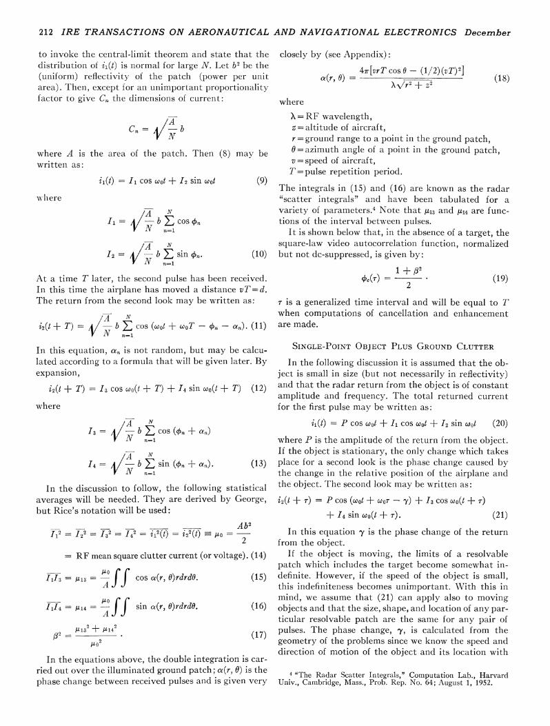
The geometry of the ground patch is shown in Fig. 1.The radar system is presumed to be in an aircraft flyingat constant speed, v, at constant altitude, z, and in a

straight line, moving a distance d in time T. The means

of looking at the ground is, of course, a pulsed RF car-

rier. It is assumed that the situation is adequately de-scribed by assuming CW transmission. The duration ofthe pulse determines the radial extent of the resolvablepatch. The antenna beam pattern is assumed to be uni-form over an angle equal to the half-power beamwidthand zero outside this angle. Therefore the resolvableground patch has an azimuthal extent equal to thebeamwidth, and a radial extent, at distances not too

Fig. 1 Geometry of ground patch.

close to the point under the airplane, approximatelyequal to c6/2, where a is the pulse duration and c is thespeed of light. It is assumed that the illuminated groundpatch, in the absence of large reflectors, is made up of a

very large number of very small radar reflectors. Theassumptions made by George in analyzing this problemare repeated here:

1) There are a large number of isotropic reflectors inthe patch giving simultaneous returns to thereceiver.

2) The probability of receiving a particular returnfrom one reflector is independent of the value ofthe return from any other reflector.

3) The phases of the returns are random about some

average position.4) No one reflector yields a return that is large com-

pared to the sum of all the others.5) The process giving rise to the fluctuation is statis-

tically stationary in time. (This restriction may bedispensed with, if desired, and statistical ratherthan time averages may be used.)

The small reflectors in the patch are assumed to be mo-

tionless. The fluctuation is caused by the motion of theairplane and is the pulse-to-pulse fluctuation that is ofinterest in this paper.

The return may be written as:

N

ii(t) = E C,, cos (coot - On)n=l

(8)

where wo is the transmitted angular frequency and 'n isa random phase angle assumed to be uniformly distrib-uted in the interval (0, 2w7r). This is the formulation usedby Rice3 in his treatment of random noise. It is possible

I S. 0. Rice, "Mathematical analysis of random noise," Bell Sys.Tech. J., vol. 23, p. 282; July, 1944, and vol. 24, p. 46; January, 1945.

zAIRCRAFT

(o,o,z) ( d,o,z)

S2

x

-r2

2111958

212 IRE TRANSACTIONS ON AERONAUTICAL AND NAVIGATIONAL ELECTRONICS December

to invoke the central-limit theorem and state that thedistribution of ii(t) is normal for large N. Let b2 be the(uniform) reflectivity of the patch (power per unitarea). Then, except for an unimportant proportionalityfactor to give C. the dimensions of current:

closely by (see Appendix):

4ir[vrT cos 0- (1/2) (vT)2]ae(r, 6) -=V2-I-zerr2 +e2

where

/ACn= ATb

where A is the area of the patch. Then (8) may bewritten as:

il(t) = Il cos coot + 12 sin coot (9)

wlhere

1, = /-bf, COS (Pn1=iN bE=°¢wA N

12=1/N bZEsinnt. (10)

At a time T later, the second pulse has been received.In this time the airplane has moved a distance vT=d.The return from the second look may be written as:

i2(t + T) b , cos (coot + woT - n- n). (11)

In this equation, a,, is not random, but may be calcu-lated according to a formula that will be given later. Byexpansion,

i2(t + T) = 13 cos wo(t + T) + I4 sin Wo(t + T) (12)

where

VA N

13 = b ,I cos (On + a,,)N n=1

14 = t N b , sin (O9n + an) (13)

In the discussion to follow, the following statistical

averages will be needed. They are derived by George,but Rice's notation will be used:

___ .__ Ab2I,2 = I22 = I32=I42 = i12(t) = i22(t)I.oo 2

= RF mean square clutter current (or voltage). (14)

1313 = -U3 = -f cos a(r, O)rdrd6. (15)

1114 = 1114 = sin a(r, O)rdrdO. (16)

=2 132 + 11142 (17)

/12

In the equations above, the double integration is car-

ried out over the illuminated ground patch; ae(r, 0) is thephase change between received pulses and is given very

X = RF wavelength,z = altitude of aircraft,r=ground range to a point in the ground patch,0=azimuth angle of a point in the ground patch,v = speed of aircraft,T=pulse repetition period.

The integrals in (15) and (16) are known as the radar"scatter integrals" and have been tabulated for a

variety of parameters.4 Note that A113 and /114 are func-tions of the interval between pulses.

It is shown below that, in the absence of a target, thesquare-law video autocorrelation function, normalizedbut not dc-suppressed, is given by:

1 + -32

2(19)

r is a generalized time interval and will be equal to Twhen computations of cancellation and enhancementare made.

SINGLE-POINT OBJECT PLUS GROUND CLUTTER

In the following discussion it is assumed that the ob-ject is small in size (but not necessarily in reflectivity)and that the radar return from the object is of constantamplitude and frequency. The total returned currentfor the first pulse may be written as:

il(t) = P cos cot + I1 cos coot + 12 sin coot (20)

where P is the amplitude of the return from the object.If the object is stationary, the only change which takesplace for a second look is the phase change caused bythe change in the relative position of the airplane andthe object. The second look may be written as:

i2(t + r) = P cos (cot + WOT - y) + I3 cos Wo(t + r)

+ I4 sin coo(t + r). (21)

In this equation -y is the phase change of the returnfrom the object.

If the object is moving, the limits of a resolvablepatch which includes the target become somewhat in-definite. However, if the speed of the object is small,this indefiniteness becomes unimportant. With this inmind, we assume that (21) can apply also to movingobjects and that the size, shape, and location of any par-

ticular resolvable patch are the same for any pair ofpulses. The phase change, y, is calculated from thegeometry of the problems since we know the speed anddirection of motion of the object and its location with

4 "The Radar Scatter Integrals," Computation Lab., HarvardUniv., Cambridge, Mass., Prob. Rep. No. 64; August 1, 1952.

(18)

Urkowitz: Performance of Airborne Moving-Target Indicators

respect to the airplane. It may easily be shown that:

4ir(Si - S2)ly= x

Si = -\/ra2 + Z2

S2 = [(ra COS Ga + VTT COS X - yr)2

+ (ra sin Ga + VTT sin 17)2 + Z2]2 (22)where

Si and S2 =the first and second slant ranges to theobject,

ra=ground range to the object (first pulse),Ga= azimuth of object (first pulse),VT =speed of object,

=direction of motion of object measuredfrom track of airplane,

T =time between observations, here equal tothe pulse repetition period, T.

The other symbols have the meanings previouslygiven for them.The representations given in (9) and (20) are just like

the representation used by Rice for random noise and asine wave plus random noise, with the probability den-sity function of the I's being normal. The video auto-correlation functions will now be derived. Rice's resultsmay be used with modifications. His representation ofthe sine-wave signal is:

P cos Pt,and at a time r later,

P cos p(t + r).

Our representation of the return from the object (calledthe signal) is

P cos coot,

and at a time T later,

P cos (coot + COOT - Y).

Thus, wherever Rice has cos pT, we put

cos (coo7 - -y).

Using Rice's formula,5 modified as described, we get thecomplete autocorrelation function after a square-lawdevice:

( p2 + 2 P' cos 2(coor -y)2 8

+ 2P24b(r) cos (coor - 7) + 2+I2(r) (23)

where, for the ground clutter,

0t(r) = ti(t)i2(t + r)

= [ ()b2 Ecosan] COS WOT

5 Rice, op. cit., sec. 4.10, (4.10-3).

+ [4 (-N) b2 E sin a,n] sin coor. (24)

t(-r) is the RF autocorrelation function of the clutterreturn. For large N,

y16(r) =/13 cCOS CoT + 1114 sin CoOT. (25)

To find the vieo autocorrelation function, the low-frequency components, including dc, of (23) are re-tained. The resulting unnormalized video autocorrela-tion function is:

cIb(r) uo2(x + 1)2 + 2x/1o2 COS (0o - y) + A102132 (26)

where

x P2/(211o) = RF signal-to-clutter power ratio

o= tan-(-).,13

The normalized video autocorrelation function is ob-tained by dividing (26) by (D(O):

T(T) =(x + 1)2 + 2x cos(Go - -y) +32

(27)(x + 1)2 + 2x + I

The subscript in the left-hand side of (27) indicates thepresence of a target. In the absence of a target, x =0,and (27) reduces to (19). For the computation of cancel-lation and enhancement, the value of T which would beused is T, the repetition interval.

FORMULAS FOR CLUTTER CANCELLATION ANDMOVING TARGET ENHANCEMENT

When (19) is substituted into (5), the result for cluttercancellation is

1Cc =

1 -12(28)

To distinguish the autocorrelation functions for station-ary and moving targets, we may use the subscripts s andm, respectively. Then, for a moving target,

Om(T) =(X + 1)2 + 2x cos (G 0 - -yin) + 132

(x+ ) +2x + 1(29)

and, for a stationary target,

(x + 1)2 + 2x cos (0G - -ys) + 12

(X+ 1)2+ 2x+ 1* (30)

When (29) and (30) are substituted into (7), the follow-ing result is obtained for moving target enhancement:

2x[1 - cos (0o - 'Yem)] + 1 - 122x[1 -cos (0GU- s)] + 132

2x[1 - cos (0o - 7m)] + 1/Cc2x[1 - cos (0o- 'Y)] + 1/cc

(31)

Eq. (31) represents a simple relationship between can-cellation and enhancement.

1958 213

s),(T) =

214 IRE TRANSACTIONS ON AERONAUTICAL AND NAVIGATIONAL ELECTRONICS December

DISCUSSIONStrictly speaking, the position of the object in the

ground patch determines the enhancement, so that thevalue of enhancement one gets depends upon where inthe patch the object is assumed to be. However, thevalues of the autocorrelation functions involved varyonly slightly over the limits of a patch (on the order of200 or 300 feet on a side), so that it doesn't matterwhere the object is in the patch. However, for the sakeof consistency it is recommended that the limits of thepatch, for the computation of (15) and (16), be takenso that the object is in the center.One may ask what distinguishes a ground patch hav-

ing a stationary target from one without a target. Theanswer is: very little if the target echo is small. If theecho is large, however, the central limit theorem cannotbe applied and the return must be treated as an addi-tional signal superimposed upon the clutter return, asis done here. The central limit theorem can be appliedin our ground clutter case because under our assumptionof uniform reflectivity and the assumption of a largenumber of scatterers, each scatterer's contribution isvery small compared to the total.

It is interesting to compare the enhancement, as de-fined by (7) and given by (31), with the velocity re-sponse usually ascribed to a single delay and subtractioncancellation system. The velocity response of such acanceller is of the form sin2 (wT/2), in power terms,where w is 27r times the Doppler frequency and is pro-portional to the radial component of target velocity andT is the radar repetition period. The response falls tozero at regular intervals and the speeds at which theyoccur are called "blind speeds." The situation with re-spect to enhancement as defined is not so simple, al-though there are similarities. First of all, note that thedenominator of (31) remains fixed when only the targetvelocity is considered. The denominator will never beexactly zero; its minimum value is I/Cc. However, sincethe clutter cancellation is usually very large, the mini-mum value of the numerator will be very small and truenulls will appear. The variation of the radial componentof target velocity is implicit in the variation of /ym, thephase change between successive pulses caused by targetmotion.These nulls occur at specific values of the radial com-

ponent of target velocity; these values for the radialcomponent may properly be called "blind speeds." Theblind speed intervals are not exactly uniform because

the pulse-to-pulse phase change is not exactly propor-tional to the radial speed. This can be seen from (22),the equations for S1 and S2.An approximate expression for the maximum value

of enhancement may be obtained in the following way.Maximum enhancement will be obtained when d0-Ym= 7w/2 and Oo= ys. Also, we shall suppose that the tar-get-to-clutter ratio is not too small. Then the numeratorof (31) will be approximately 2x, and the denominatorwill be 1Cc. Then, the maximum enhancement is givenby:

Emax - 2xCG. (32)

APPENDIXEq. (18) may be derived in the following way. The

phase change between pulses is given by (Fig. 1):

4ra (r, 0) = (sl - S2).

Now,

S =2 2 + y2 + z2 = r2 + z2

S2= (X-d)2 + y2 + z2

but,

d = vT

x = r cos6.

Therefore,

S22 r2 + z2 - 2vTr cos 0 + v2T2S- = (r2 + Z2)1/2

(1 -2vTr cos6 + V2T2 1/2](\1 ~r2+ z2 (34)

Now, by the binomial expansion, if a<<K, then

(1 - a)I2I 1 -a

2(35)

where higher powers of a are neglected. Applying thebinomial expansion to the square root inside the brack-ets of (34), one obtains:

vTr cos 0- (1/2)(vT)2S1 - S2

(r2 +I z2)112(36)

When (36) is substituted into (33), the result is (18).

(33)