An IntERPREtAtIOn OF An AFFInE tERM StRUCtURE MODEL FOR … · An IntERPREtAtIOn OF An AFFInE tERM...

An interpretation of an affine… / J. Marcelo Ochoa 155

An IntERPREtAtIOn OF An AFFInE tERM StRUCtURE MODEL FOR ChILE*

J. maRceLo ochoa∗∗

Abstract

This paper attempts to provide an economic interpretation of the factors that drive the movements of interest rates of bonds of different maturities in a continuous-time no-arbitrage term structure model for Chile. The dynamics of yields in the model are explained by two latent factors, namely the instantaneous short rate and its time-varying central tendency. The model estimates suggest that the short end of the yield curve is mainly driven by changes in first latent factor, while long-term interest rates are mainly explained by the second latent factor. Consequently, when examining movements in the term structure, one should think of at least two forces that hit the economy: temporary shocks that change short-term and medium-term interest rates by much larger amounts than long-term interest rates, causing changes in the slope of the yield curve; and long-lived innovations which have persistent effects on the level of the yield curve.

Resumen

Este artículo intenta ofrecer una interpretación económica a los factores latentes que determinan los movimientos del retorno de bonos de diferente plazo en un modelo de la estructura de tasas de interés en tiempo continuo y con ausencia de arbitraje para Chile. En el modelo, dos factores latentes explican la dinámica de las tasas de interés, la tasa de interés instantánea y su tendencia central estocástica. Los resultados sugieren que el tramo corto de la estructura de tasas de interés se explica primordialmente por cambios en el primer factor, mientras que el segundo factor explica el tramo más largo de la estructura de tasas. Por lo tanto, si uno considera los factores que explican los movimientos de la estructura de tasas de interés, debería pensar en al menos dos tipos de innovaciones presentes en la economía: innovaciones temporarias que provocan cambios en las tasas de interés de corto y mediano plazo, mucho mayores que los experimentados por tasas de interés de largo plazo, e innovaciones persistentes que tienen efectos sobre el nivel de la estructura de tasas.

keywords: Affine term structure model, yield curve, Kalman filter,

JEL classification: C33, E43, E44, E2, G12.

∗ I am grateful to Rómulo Chumacero for his insightful suggestions and comments and to Viviana Fernández, Juan Pablo Medina and Rafael Romero for helpful discussions. I am, however, responsible for any errors and for the views expressed in the paper. This paper is based on my Master thesis in Economics at the University of Chile.

∗∗ Banco Central de Chile, Gerencia de Investigación Económica. e-mail: [email protected].

Estudios de Economía. Vol. 33 - Nº 2, Diciembre 2006. Págs. 155-184

Estudios de Economía, Vol. 33 - Nº 2156

1. IntroductIon

Affine no-arbitrage dynamic term structure models are “the model[s] of choice in finance” (Diebold, Piazzesi, and Rudebusch 2005). These models employ a structure that consists of a small set of factors that characterize the yield curve, providing a parsimonious representation of the yield curve. At the same time they impose restrictions to ensure that yield dynamics are consistent in the cross-sec-tion and in the time series dimension (Dai and Singleton 2000, Piazzesi 2003). Even though these models provide a useful statistical description of the yield curve, they offer little insight of what the latent factors are, their relationship to macroeconomic variables, or the forces that drive its movements.

In this paper I attempt to provide an economic interpretation of the factors that drive the movements of interest rates of bonds of different maturities in a continuous-time no-arbitrage term structure model. Following Jegadeesh (1996) and Balduzzi (1998), the model I use in my analysis assumes the existence of a stochastic discount factor, which is governed by two latent factors with a proper economic interpretation. The first latent factor is the instantaneous short-term interest rate, and the second factor is the time-varying stochastic mean of the instantaneous short rate, capturing the notion that short rates display short-lived fluctuations around a time-varying rest level. This model generalizes the continu-ous-time term structure model presented in Vasicek (1977), but it is nevertheless solvable in closed form. Under this framework, bond yields are linear or affine functions of the latent factors, with restrictions on the cross-sectional and time-series properties of the yield curve that rule out arbitrage strategies.

while most of the related literature has focused on the analysis of the U.S. economy, little attention has been paid to emerging markets. I estimate the proposed model using monthly information on index-linked securities issued by the central bank and traded in the Chilean bond market from January 1990 through March 2006. Compared to developed economies, the Chilean fixed-income bond market is not underdeveloped, and Central Bank bonds are by far the most traded as well as the most liquid fixed-income securities (see Braun and Briones 2006). Nevertheless, the analysis of an emerging economy comes along with several estimation challenges. Most studies use zero-coupon yields that are estimated from prices of coupon bonds using one of the interpolation methods proposed by Fama and Bliss (1987) and McCulloch and kwon (1993). Typical implementation of these methods requires a rich set of bond prices with different maturities, which are unavailable in many emerging markets where there is a substantial number of ‘missing bond yields’. To overcome this problem, I rely on an extended version of the kalman filter and maximum-likelihood to estimate the unobservable state variables and the model parameters using cross-sectional/time-series data of zero-coupon and coupon bond prices. Using this approach, I am able to estimate the zero-coupon term structure even for days where bonds with only few maturities are traded, while at the same time the kalman filter allows the state variables to be handled correctly as unobserv-able variables.1

1 Babbs and Nowan (1999) provide a generalization of the kalman filter to estimate generalized Vasicek term structure models, and Cortázar, Schwartz and Naranjo (2003)


The model estimates suggest that the instantaneous rate is more volatile and exhibits short-lived deviations from its time-varying mean, while the time-varying central tendency exhibits a weak reversion to its long-run value and a volatility less than half that of the short rate. According to the factor loadings implied by the estimated parameters, the very short end of the yield curve is driven by the first latent factor, but as the term to maturity increases the central tendency starts driving the movements in the yield curve, playing an important role at explaining the evolution of long-term interest rates. Consequently, a shock to the first latent factor increases short-term and medium-term interest rates by much larger amounts than the long-term interest rates, so that the yield curve becomes less steep (i.e., experiences a decrease in its slope). Thus, it is reasonable to interpret this short-lived shock as a temporary positive shock to the economy which increases temporarily production possibilities. On the other hand, a shock to the time-varying mean translates into an increase in short-term and long-term yields, changing the level of the yield curve. Therefore, a second source of shocks that moves the yield curve can be related to long-lived innova-tions which will induce a persistent change in the level of the yield curve, like a persistent (almost permanent) positive shock to productivity.

My work is more closely related to recent economics and finance papers exploring the macroeconomic determinants of the unobservable factors, and to macro-finance modeling which explicitly incorporates macroeconomic variables into multi-factor yield curve models. For instance, wu (2001) and Piazzesi (2005) relate monetary policy shocks to temporary changes in the factor that influences the slope of the yield curve (slope factor), since monetary policy surprises affect short rates more than long ones. Ang and Piazzesi (2003) examine the influ-ences of macroeconomic variables and latent factors that jointly determine the term structure of interest rates. They find that inflation and real activity have a significant impact on medium-term bond yields (up to a maturity of one year), but most of the movements in long-term yields are still accounted for by the unobservable factors. while most of these papers agree on the effects of mac-roeconomic variables on the slope of the yield curve, there are still conflicting results when explaining the movements of the level of the yield curve. Diebold, Rudebusch and Aruoba (2006) obtain more favorable results using a Nelson-Siegel model combined with a VAR-model for the macroeconomy. They find that inflation is closely related to the factor that influences the slope of the yield curve, while the factor that changes the level of the yield curve (level factor) is highly correlated with real activity. Using different modeling strategies, Rudebusch and wu (2004) and Dewatcher and Lyrio (2006) interpret the slope factor as the cyclical response of the central bank to changes in the economy. while Rudebusch and wu (2004) argue that the level factor reflects market participants’ view about the inflation target of the central bank, Dewatcher and Lyrio (2006) link this factor to long-run inflation effects.

The early literature investigating the term structure of interest rates in Chile has relied on the parametric model proposed by Nelson and Siegel (1987) (Herrera and Magenzo 1997, zuñiga and Soria 1998 and Lefort and walker 2000), however,

present an application of this methodology for a market with low-frequency transactions, namely Chile.


this type of model does not acknowledge that bond yields need to be consistent, giving rise to term structure estimates which allow arbitrage opportunities. The studies of Parisi (1998, 1999) and zuñiga (1999b) go further and investigate the ability of one-factor no-arbitrage models in explaining the short-term interest rate, while zuñiga (1999a) and Cortázar et. al. (2003) provide estimates of multi-factor models. They find that no-arbitrage models outperform parametric specifications (Cortázar et. al. 2003) and more simple autoregressive models (Parisi 1999). Fernandez (2001), on the other hand, uses a semi-parametric specification of a one-factor no-arbitrage model to study the empirical properties of the term structure of interest rates. More recently, Morales (2005) analyzes the impatc of macroeconomic variables on the term structure of interest rates using a Nelson-Siegel model augmented by macroeconomic variables. His findings suggest that economic activity as well as monetary policy shocks impact the yield curve. In contrast to the previous literature for Chile, I don’t only present estimates of the term structure of interest rates, but also attempt to give an economic interpreta-tion to the model estimates. Moreover, I characterize the way in which shocks to the factors behind the movements of the term structure change interest rates of different maturities, and provide a possible interpretation to this innovations in a internally consistent model using model-based impulse-response functions.

The rest of the paper unfolds as follows. In Section 2 I present the continu-ous-time no-arbitrage term structure model. In Section 3 I present the state space formulation of the model and the estimation of the parameters by means of the kalman filter. I also present an interpretation of the estimated parameters and discuss the reliability of the model-based yield curves obtained. In Section 4 I use impulse-response functions implied by the affine term structure model to discuss the sources of shocks that move the yield curve and their possible economic interpretation. Section 5 concludes.

2. AmodeloFthetermstructure

Here I introduce the framework that I use for modeling the term struc-ture of interest rates. First, I present several important relationships on asset pricing. Then, I present the solution to the no-arbitrage term structure model governed by two latent factors. Are two factors enough? Even though the work of Litterman and Scheinkman (1991) finds that almost all of movements in various US Treasury bond yields are captured by three unobservable factors, the study of Diebold, Rudebusch and Aruoba (2006) find that two factors may suffice to capture the time-series variation in yields at a monthly frequency, since the first two principal factors account for almost 99% of the movements of yield-curve variation. The third factor is found unimportant since it is related to heteroskedasticity, and yields exhibit little heteroskedasticity at monthly frequency. The third factor is more important at daily and weekly frequencies (Ang, Piazzesi, and wei 2006).

�.� background issues on asset pricing

Let P(t, T) denote the price at time t of a zero-coupon bond maturing at time T. Assuming, without loss of generality, that the bond has a face value


equal to one and its yield to maturity with continuous compounding is equal to R(t, T), its price can be written as,

(1) P t T T t R t T( , ) = [ ( ) ( , )]exp − −

and the yield to maturity on this zero-coupon bond is equal to,

(2)

R t TP t T

T t( , ) =

( , )−−

log

Using these results, one can define the instantaneous short rate as,

(3)

r R t TP t T

T tt T t T t= ( , ) =

( , )lim lim

log→ →

−−

Similarly, the price of a coupon bond paying t coupons until the maturity date can be written as a portfolio of t zero-coupon bonds,

(4)

P t T C P t t i

C iR t t

c

ii

ii

( , ) = ( , )

= [ ( ,

=1

=1

t

t

∑

∑

+

− +exp ii)]

where t = T–t is also the time to maturity of the coupon bond (see Campbell, Lo, and Mackinlay 1997).

�.� An affine term structure model

In an arbitrage free-environment and with a positive stochastic discount factor equal to Lt, the price at date t of a zero-coupon bond paying one unit of account at time T can be expressed as,

(5) P t T tT

t

( , ) = EΛΛ

where Et is the expectation taken conditional on time-t information. Following the standard asset-pricing theory, I assume that the stochastic discount factor is governed by the following process,

(6) d r dt dt t t t'

tΛ Λ Λ= − − λ W

where λ = [λ1, λ2]’ is a vector containing the market prices of risk which are assumed to be constant over time.


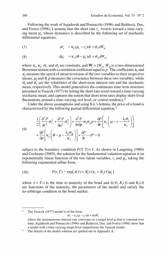
Following the work of Jegadeesh and Pennacchi (1996) and Balduzzi, Das, and Foresi (1998), I assume that the short rate rt reverts toward a time-vary-ing mean µt, whose dynamics is described by the following set of stochastic differential equations,

(7) dr r dt dWt t t t= ( )1 1 1κ µ s− +

(8) d dt dWt t tµ κ q µ s= ( )2 2 2− +

where κ1, κ2, s1, and s2 are constants, and wt = [W1t, W2t is a two-dimensional Brownian motion with a correlation coefficient equal to r . The coefficients κ1 and κ2 measure the speed of mean reversion of the two variables to their respective means, µt and q, r measures the covariance between these two variables, while s1 and s2 are the volatilities of the short-term interest rate and the stochastic mean, respectively. This model generalizes the continuous-time term structure presented in Vasicek (1977) by letting the short-rate revert toward a time-varying stochastic mean, and captures the notion that short-term rates display short-lived fluctuations around a time-varying rest level, or central tendency.2

Under the above assumptions and using It o ’s lemma, the price of a bond is characterized by the following partial differential equation,3

(9)

1

2

2

2 12

2

2 22

2

1 2

∂∂

+ ∂∂

+ ∂

∂ ∂+ ∂P

r

P P

r

Psµ

sµ

s s r∂∂

− −

+ ∂∂

− −

rr

P

κ µλ sκ

µκ q µ

λ s

11 1

1

22 22

2

= 0κ

+ ∂∂

−P

trP

subject to the boundary condition P(T, T)= 1. As shown in Langetieg (1980) and Cochrane (2005), the solution for the fundamental valuation equation is an exponentially linear function of the two latent variables, rt and µt, taking the following exponential-affine form,

(10) P t T A B r Bt t( , ) = [ ( ) ( ) ( ) ]1 2exp t t t µ+ +

where t = T–t is the time to maturity of the bond and A(t), B1(t) and B2(t) are functions of the maturity, the parameters of the model and satisfy the no-arbitrage condition in the bond market.

2 The Vasicek (1977) model is of the form, dr r dt dWt t t= ( )1κ µ s− +

where the instantaneous interest rate converges to a target level µ that is constant over time. Jegadeesh and Pennacchi (1996) and Balduzzi, Das, and Foresi (1998) show that a model with a time-varying target level outperforms the Vasicek model.

3 The details of the model solution are spelled out in Appendix A.


Equations (9) and (10) determine the solution for the functions A(t), B1(t) and B2(t) in terms of a set of ordinary differential equations, which have a solution equal to,

B

B

11

1

22

2

( ) =( ) 1

( ) =( ) 1 (

tκ tκ

tκ tκ

exp

exp exp

− −

− −−

−− − −−

+∫

κ t κ tκ κ

t s st

1 2

1 2

0 12

12

22

2

) ( )

( ) =1

2

exp

A B B 221 2 1 2 1 1 1 2 2 2 2 2+ − − +

B B B B B dss s r λ s λ s κ q

Using equation (2) and (10) we can write the yield of a bond maturing t periods ahead as,

(11) R t T A B r B

a b

t t( , ) =1

[ ( ) ( ) ( ) ]

= ( ) ( )

1 2

1

− + +

+t

t t t µ

t t rr bt t+ 2 ( )t µ

where a(t)= –A(t)/t, b1(t)= –B1(t)/t and b2(t)= –B2(t)/t. In this model, bond yields are linear functions of the state variables, rt and µt. Therefore, it belongs to the family of affine term structure models, in which zero-coupon bond yields, their physical dynamics and their equivalent martingale dynamics are all affine (constant-plus-linear) functions of an underlying vector of state variables.4

Using equation (3), one can see that the instantaneous short rate is given by,

(12) limt

t→

+0

( , ) =R t t rt

and the long-term rate is equal to the mean of the stochastic time varying long-term factor q adjusted by risk premia,

(13) limt

t qλ sκ

λ sκ

s sκ→∞

+ − − −+

−R t t( , ) =2

2 2

2

1 1

1

12

22

12

ss s rκ κ1 2

2 1

Notice that the time-varying mean of the first latent factor, µt, does not affect the short end of the yield curve, since its loading starts at zero for the instantaneous interest rate (i.e., lim

tt

→0 2 ( ) = 0B ). However, it does affect yields of longer maturities, influencing the long-end of the term structure.

4 See Piazzesi (2003) for a review of affine models of the term structure.


3. estImAtIon

3.� Data

In this paper I use three types of instruments to estimate the yield curve; pure discount bonds, which make a single fixed payment at the maturity date; coupon bonds which make coupon payments at equally spaced intervals until the maturity date, in which the face value is also paid and, coupon bonds paying both, the face value and the coupon rate, in each coupon payment.

I use end-of-month price quotes for index-linked instruments issued by the Central Bank of Chile, which have both their coupon and principal payments linked to the Unidad de Fomento (UF), from January 1990 through March 2006. The UF is a unit of account that varies according to past inflation, and is not perfectly correlated with current inflation. For short-maturity instruments, UF-linked yields cannot be considered real yields, but as the maturity of the instrument increases these yields approximate real interest rates more closely (see Chumacero 2002).

The database contains 4,472 observations on pure-discount bonds (Pagare Reajustable del Banco Central), and semi-annual amortizing coupon bonds (Pagare Reajustable con Cupones and Bonos del Banco Central de Chile). Over the sample period, each month contains an average of twenty seven observa-tions. In early years, however, the number of index-linked bonds outstanding is very small, resulting on a median of 8 monthly observations over 1990 and 1991. During these first two years, the maturity of coupon bonds, as well, is confined to values that range from fifteen to twenty semesters and zero-coupon bonds which have maturities of less than one year. As we move forward in time, the maturity of traded coupon bonds diversifies ranging from 1 month to 40 semesters (see Figure 1).

FIGURE 1END-OF-MONTH AVAILABLE DISCOUNT AND COUPON BONDS OVER THE

SAMPLE PERIOD. A POINT REPRESENTS A BOND AVAILABLE FOR THE CORRE-SPONDING MATURITY AND TIME PERIOD.


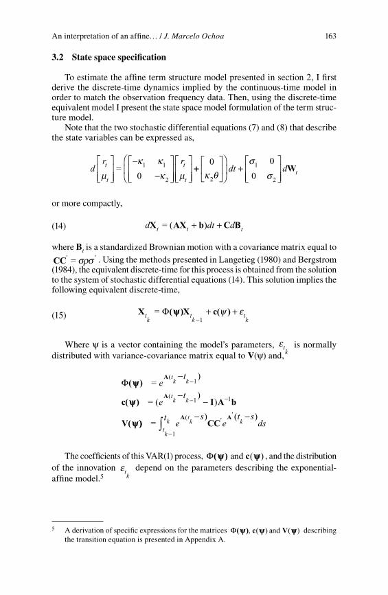
3.� State space specification

To estimate the affine term structure model presented in section 2, I first derive the discrete-time dynamics implied by the continuous-time model in order to match the observation frequency data. Then, using the discrete-time equivalent model I present the state space model formulation of the term struc-ture model.

Note that the two stochastic differential equations (7) and (8) that describe the state variables can be expressed as,

dr rt

t

t

tµκ κ

κ µ

−

−

=0

1 1

2

++

+

0 0

02

1

2κ q

ss

dt d tW

or more compactly,

(14) d dt dt t tX AX b C B= ( )+ +

where bt is a standardized Brownian motion with a covariance matrix equal to

CC' '= srs . Using the methods presented in Langetieg (1980) and Bergstrom (1984), the equivalent discrete-time for this process is obtained from the solution to the system of stochastic differential equations (14). This solution implies the following equivalent discrete-time,

(15) X ( )X c( )tk

tk

tk

=1

Φ ψψ−

+ +ψ ε

where ψ is a vector containing the model’s parameters, εtk

is normally distributed with variance-covariance matrix equal to V(ψ) and,

Φ( )

c( ) I A b

V(

A

A

ψψ

ψψ

ψψ

=)

= ()

)

(1

(1 1

et

et

tk k

tk k

−

−−

−

− −

)) CCA A

=) ( )

1

(

tk

ktk '

'kt

es

et s

ds−

∫− −

The coefficients of this VAR(1) process, Φ( )ψψ ψψand c( ) , and the distribution of the innovation εt

k depend on the parameters describing the exponential-

affine model.5

5 A derivation of specific expressions for the matrices Φ( )ψψ ψψ ψψ, c V( ) and ( ) describing the transition equation is presented in Appendix A.


To complete the state space representation of the model, I present the mea-surement equation which relates the theoretical yields and the latent factors describing the model. At time tk, the data is comprised by Nk bond prices of different maturity denoted by

Ptk

k k Nk

P P P= ( , , , )1 2 K for k=1, k, T. The set

of instruments contains both, zero-coupon and coupon bonds with maturities that vary over time. I assume that there are discrepancies between observed prices and their theoretical counterparts explained by exogenous factors such as non-synchronous trading, rounding of prices, and bid-ask spreads. Therefore, in the presence of measurement errors we need to distinguish between the theoretical term structure given by (10) and observed prices. Assuming that measurement errors are additive and normally distributed, theoretical and observed prices are related by,

(16) P Q , X vtk

tk

tk

= ( )ψψ +

where v Htk

k:N (0, ( ))ψψ is the measurement error, the vector ψψ contains

the unknown parameters of the model, Xtk

is a vector containing the two state

variables of the model (i.e., X=r, m) X = ( , )r 'µ ), and the i–th row of Q , X( )ψψ tk

is equal to,

Q , Xi tk

i i tk

i tk

A B r B( ) = [ ( ) ( ) ( ) ]

=

1 2ψψ exp

ex

t t t µ+ +

pp[ ( ) ( ) ]A i i'

tk

t t+ B X

when the i–th bond is a zero-coupon bond and equal to,

Q , X B Xi tk j

i

ij'

tk

C A j j( ) = [ ( ) ( ) ]=1

ψψt

∑ +exp

when the i–th bond is a coupon bond paying ti coupons until the maturity.

The measurement equation (16) plus the transition system describing the state variables form the non-linear state space model describing the term structure of interest rates.

3.3 Extended kalman Filter

Even though the conventional kalman filter cannot be used in the presence of non-linear measurement and/or transition equations, an approximate filter can be obtained by linearizing the non-linear measurement equation and then applying the extended kalman filter presented in Harvey (1990). The original non-linear measurement equation (16) can be approximated using a Taylor expansion around the conditional mean of the state variables,

(17) P , X Z , X X vtk

tk k

tk k

tk

kd t t= ( | ) ( | )1 1

ψψ ψψ− −

+ +


where Xtk k

t|1−

is the conditional mean of the state variables given the information

set available at tk, d , X( | )1

ψψtk k

t−

is an Nk-vector with the i– th row given by,

d tt

'i tk k

tk k

tk

tk

= ( | )( | )

|1

1Q , XQ , X

XXψψ

ψψˆ

ˆˆ

−

−−∂

∂ttk −1

and Z , X( | )1

ψψtk k

t−

is an Nk × 2matrix with rows equal to

ZP t

'i

tk k

tk

=( | , )

.1∂

∂−

X

X

t

Using the linear approximation of the measurement equation (17) and the transition equation (15), the parameters of the model can be estimated using the extended kalman filter algorithm discussed in Harvey (1990). This algorithm consists of a sequence of two steps, a prediction and an update step. The predic-tion step yields the estimator of the state variables given by,

(18) ˆ ˆ ˆX X c( ) ( )X

tk k

tk

tk

tk

t| = ( | ) =1 1 1− − −

+E Ξ ψψ ΦΦ ψψ

with a mean square error (MSE) equal to,

F X X X Xtk k

tk

tk k

tk

tk k

't t t| = ( | )( | ) |

1 1 1− − −− −E ˆ ˆ Ξtt

k

tk

'

−

−

+

1

1= F FF V

where the expectation is based on the available information up to time tk–1 represented by Ξt

k −1.

In the update step, we use the additional information given by Ptk

to obtain a more precise estimator of Xt

k,

(19)

ˆ ˆ

ˆ

X X

X F Z ZF

tk

tk

tk

tk k

tk k

'tk

t t

= ( | )

= | | 1 ( |1

E Ξ

−+ − tt t

k

'tk

tk k

− + −

−

−1 ) ( | )1

1Z H P Q , XΨ ˆ

with a MSE matrix equal to,

F X X X X

F

tk

tk

tk

tk

tk

'tk

tk k

t

= ( )( ) |

= |

E − −

ˆ ˆ Ξ

−− − − − + −−

1 | 1 ( | 1 ) | 11F Z ZF Z H ZF

tk k

'tk k

'tk k

t t t


Once we obtain estimates of the state variables (i.e., Xtk

) using informa-tion about the observed bond prices, we can evaluate the likelihood function using the prediction error decomposition (see Harvey 1990 for details). Then, the log-likelihood function is given by,

(20) k

T

tk t

k

k

k

n

fn N

=1 =1

( | ) ==1 2

(2 )1

2∑ ∑ ∑− −log log lP Ψ π oog | |1

2 =1

1S v S vkk

n

tk

k tk

'− ∑ −

where, v P , X

ZF Z H

tk

tk

tk k

k tk k

'

t

t

= ( | )

= | 1

1−

− +−

Q y ˆ

S

3.4 Estimation results

I estimate the term structure model using the extended kalman filter algorithm and assuming that prices are observed with an error. I aggregate bonds into five categories to obtain a parsimonious covariance matrix of the measurement errors. Each group is assumed to have the same measurement error, therefore, the covariance matrix of the measurement errors hk (ψ) is a diagonal matrix with five different elements characterizing the variance of each group, hi. The first group contains discount bonds which have maturities less or equal to one year. The remaining four groups comprise coupon bonds with maturities up to five years, between six and ten years, between eleven and fifteen years, and above sixteen years, respectively.

Unlike the standard practice, I treat the factors r and µ as unobservables, and do not approximate the instantaneous rate using an observed short-term interest rate or the time-varying mean using observed yields as in Chan et al. (1992), Longstaff and Schwartz (1992), and Balduzzi et al. (1998). while ap-proximating latent factors with observable yields is convenient, note that yields of any finite-maturity depend on both factors, r and µ, as well as on the model parameters we are trying to identify.

Table 1 presents the estimation results. with exception of the coefficient capturing the market price of risk of the central tendency, λ2, all parameter estimates are significant at conventional values. Both, the instantaneous interest rate and the time-varying central tendency present statistically significant rever-sion toward its central tendency. However, the mean reversion and the volatility of the instantaneous rate are considerably higher than the coefficients estimated for its time-varying mean. Therefore, the short-term rate is more volatile and returns faster to its time-varying mean, while the central tendency exhibits a weak reversion to its long-run value and a volatility less than a half that of the short-rate. The mean-reversion parameters imply a half-life of about 1 year for the short-rate, while the estimated half-life for the time-varying mean is 14.83 years (see Figure 3).

These results suggest that the time-varying mean can be interpreted as the level of interest rate that would prevail after ongoing temporary imbalances


in the economy –those that are expected to dissipate over the short-run– work themselves through. In contrast, fluctuations of the first latent state variable rt around its time-varying mean reflect shorter-lived shocks. The model-based equilibrium real interest rate, which abstracts from both short-lived and long-lived shocks, is equal to R∞ = 2.47 percent in semestral base or R∞ = 4.94 percent in an annual base. The estimate of q, the steady-state value of the short-rate and the central tendency, is statistically significant and equal to 2.95 percent in semestral base or 5.92 percent in annual terms.

The estimated loadings of the two factors driving the yield curve provides an insight on how each factor dynamics translates into movements of the yield curve. In order to give an interpretation of the estimated factor loadings, note that one can rewrite equation (11) as,

R t t a R b r bt t( , ) = ( ) ( ) ( ) ( )1 1 2+ ∞ + +t t t t µ

where R R t t( ) = ( , )∞ +→∞

limt

t . Figure 2 depicts the loadings on the long-term interest rate a1(t), on the short-term interest rate b1(t), and on the time varying long-term rate b2(t) along different maturities, calculated using the estimates presented in Table 1. The very short end of the yield curve is driven by the first latent factor rt. The loading associated to the short-term interest rate b1(t) starts at 1 and decays monotonically as the term to maturity increases reaching a value close to zero at long maturities. In contrast, as the term to maturity increases, the central tendency µt becomes a central factor behind the movements of the long end of the yield curve as well as intermediate maturities.

FIGURE 2 ESTIMATED FACTOR LOADINGS IN THE AFFINE TERM STRUCTURE MODEL,


TABLE 1MAXIMUM LIkELIHOOD ESTIMATES (1990:01-2006:03)

Parameter Estimate Parameter Estimate

κ1 0.2959 h1 0.01645(0.0195) (0.0040)

s1 0.0090 h2 0.5808(0.0006) (0.0298)

λ1 –0.2686 h3 0.7498(0.1566) (0.0254)

κ2 0.0265 h4 0.0793(0.0031) (0.0064)

s2 0.0040 h5 1.9466(0.0002) (0.1280)

λ2 0.0140(0.0232)

r –0 .1480(0.0856)

q 0.0295(0.0058)

Half-life r 1.0046 years R(∞) 0.0247

Half-life µ 14.8333 years

Note: The table reports maximum likelihood estimates of an affine term structure model described by,

dr r dt dW

d dt dWt t t t

t t t

= ( )

= ( )1 1 1

2 2 2

κ µ sµ κ q µ s

− +

− +

using monthly data on zero and coupon bonds for the 1990:01-2005:03 period. The estimates of the measurement equation error covariance matrix hi are multiplied by 102. The time unit t is expressed in semesters, therefore the model-based yields are in semestral base.

These characteristics of the model produce model-based yield curves that are capable to reproduce some important stylized facts. The higher volatility and lower persistence of the instantaneous short rate compared to that of the central tendency translates into a higher volatility at the short end than at the long end of the yield curve, plus more persistent long interest rates than short interest rates (see Table 2). The dynamics of the factors behind the term structure and the estimated parameters also produce yield curves with a variety of shapes over time, including downward sloping, upward sloping, and hump-shaped, and at the same time produces yields that rule out arbi-trage possibilities between bonds of different maturities (see Figure 4). Even though the model imposes restrictions on the cross-sectional and time-series properties of the yield curve in order to rule out arbitrage possibilities, the model fits quite well the observed yield-to-maturity of zero and coupon bonds (see Figure 5).


FIGURE 3ESTIMATED LATENT FACTORS rt AND µt IN ANNUAL BASE OVER 1990:01-2006:03

TABLE 2YIELD CURVE ESTIMATES DESCRIPTIVE STATISTICS (1990:01-2006:03)

Maturity Mean Std. dev. Minimum Maximum Vt+12

1 month 4.863 3.026 –2.594 12.159 1.797

6 months 4.921 2.882 –2.069 11.794 1.796

1 year 5.021 2.637 –1.157 11.161 1.792

2 years 5.177 2.275 0.2367 10.193 1.812

3 years 5.293 2.03 1.227 9.512 1.839

4 years 5.382 1.858 1.74 9.349 1.862

5 years 5.453 1.731 1.838 9.346 1.887

6 years 5.509 1.633 1.937 9.325 1.904

7 years 5.556 1.555 2.034 9.291 1.916

8 years 5.594 1.49 2.118 9.249 1.93

9 years 5.625 1.434 2.203 9.2 1.937

10 years 5.651 1.384 2.286 9.147 1.949

15 years 5.723 1.193 2.666 8.848 1.968

20 years 5.738 1.053 2.977 8.539 1.979

Note: Descriptive statistics for model-based monthly yields at different in annual base. The last column presents the variance ratio defined as, V

k

var y y

var y ytt t

t t+

+

+

−−12

12

1

=1 ( )

( ).


The model estimates also produce an average yield curve that is increasing and concave (see Figure 6). To understand why, note that the market price of risk of the short-term interest rate imply the following risk premia for a discount bond maturing in t periods,6

λs

λ sκ t

κ11

1 11

1

=1 ( )

P

P

r

∂∂

−− −

exp

The sign of the risk premium es equal to minus the sign of the respective market price of risk, and the magnitude of the premium is an increasing function of bond maturity. The estimate of λ1, the market price of risk of the short-term interest rate, is negative and statistically significant. This implies that a bond’s interest rate risk premium is positive and increasing with bond’s maturity, sug-gesting that the yield curve is usually upward sloping.

FIGURE 4YIELD CURVES IN ANNUAL BASE ESTIMATED USING THE ESTIMATES OF AN

AFFINE TERM STRUCTURE MODEL FOR THE 1990:01-2006:03 PERIOD

Finally, the correlation between changes in the short rate and its time-vary-ing mean r is negative and statistically significant. The correlation might be interpreted as a link between agents expectation of future economic conditions and changes in the short-rate. The intuition is straightforward. Suppose the economy is in a growth stage, and the monetary authority increases the short-term interest rate in an effort to avoid an overheating of the economy. Then, if movements in the short rate are pro-cyclical and agents believed that a hike in the short rate signals future adverse economic conditions, there is an incentive to sacrifice today’s consumption to buy long-term bonds that pays off in the bad

6 See Pennacchi (1991) and Jegadeesh and Pennacchi (1996) for a derivation.


times. This increase in the demand for long-term bonds will bid up their price and lower long-term yields, resulting in a negative correlation between r and µ. The model also implies that a downward sloping yield curve not only indicates good times today, but bad times tomorrow. Therefore, when agents expect a recession, short-term rates will increase, while long rates will decrease.7

FIGURE 6MODEL-BASED AVERAGE YIELD CURVE IN ANNUAL BASE

FOR THE 1990:01-2006:03 PERIOD

7 See Harvey (1988), Estrella and Hardouvelis (1991), Plosser and Rouwenhorst (1994), kamara (1997), Chapman (1997), Estrella and Mishkin (1998), Hamilton and kim (2002), Berardi and Torous (2005) and Ang, Piazzesi, and wei (2006) for a more detailed explanation of the information content of the shape of the term structure about economic activity.

FIGURE 5MODEL-BASED YIELD TO MATURITY (CONTINUOUS LINE) AND THE OBSERVED

YIELDS OF TRADED INSTRUMENTS (CIRCLE POINTS) IN ANNUAL BASE

(a) Yield-to-maturity on September, 1993 (b) Yield-to-maturity on March, 2002


4. moVementsIntheyIeldcurVe

The yield curve might move due to changes in announcements of unemploy-ment or inflation, changes in market participants’ risk aversion aroused from perceived changes in the prospects for continued economic growth, or due to changes in other economic variables (Bliss 1997). In the model presented above changes in the instantaneous interest rate and the its time-varying central ten-dency drive changes in interest rates of different maturities to varying degrees. Therefore, it is reasonable to think that these latent factors should capture the economic factors influencing interest rates and the changes in the underlying determinants of the term structure of interest rates. Here, I discuss how the term structure of interest rates changes in response to new information about rt and µt using impulse-response functions implied by the affine term structure model. Additionally, I attempt to provide an economic interpretation of these shocks.8

Let me start by analyzing the effect of one standard innovation of the instan-taneous interest rate and how it translates into movements of the yield curve. The first two panels of Figure 7 exhibit the response of the instantaneous short-rate rt and its time-varying mean µt to an innovation in the first latent factor. Figure 8 presents the impulse-response functions of selected yields, the term structure at its initial value, and one month and 5 years after a one standard deviation of rt. The results show that the instantaneous rate rt increases imme-diately after the shock and decays monotonically returning to its initial value. On the other hand, the central tendency µ decreases slightly due to the negative correlation between the two state variables, but the confidence intervals indicate that this response is not statistically significant. As the loadings of each factor suggest, the shock to the instantaneous interest rate increases short-term and medium-term interest rates by much larger amounts than long-term interest rates. Consequently, the yield curve initially becomes less steep, presenting a decrease in its slope. The yield curve returns back to its initial position five years after the shock initiated (see Figure 8).

The movements in yields in response to this shock have an intuitive explana-tion. To better understand the following discussion, recall that the basic asset pricing model predicts that the price of a discount bond maturing in t periods is given by,

(21) P t TU c

U ctt

t

( , ) =( )

( )βt tE

′′

+

where ′U ct( ) is the marginal utility of consumption, 0 < β < 1 denotes the subjective discount factor, and Et is the expectation conditional on information available at time t. Under this framework, interest rates reflect the rate at which people are willing to trade consumption today for consumption tomorrow (Altug and Labadie 1994).

8 Appendix B contains the analytical derivation of the model-based impulse-response functions and their respective standard errors.


FIGURE 7ESTIMATED IMPULSE-RESPONSE FUNCTIONS OF THE INSTANTANEOUS SHORT RATE AND THE CENTRAL TENDENCY (SOLID LINE) ALONG 95 PERCENT CONFI-

DENCE BANDS (DOTTED LINES)

(a) Response of rt to a one std. dev. of rt (b) Response of µt to a one std. dev. of rt

(c) Response of rt to a one std. dev. of µt (d) Response of µt to a one std. dev. of µt

A shock that temporarily increases short-term and medium-term yields can be interpreted as a temporary positive shock to the economy which increases production possibilities. Intuitively, after the realization of this shock agents will face an increase in their consumption, but considering that this gain will eventually die out, economic agents will save part of the output and invest into capital in order to smooth their consumption (de Haan 1995). Therefore, the expected growth rate of consumption is expected to be positive in the short-term and medium-term, implying an initial increase in the slope of the yield curve. However, as agents start to dissave, interest rates will fall back to their long-term level and consumption growth will return to its steady-state level. This result is consistent with the results of Rendu de Lint and Stolin (2003) who find that a temporary productivity shock in a simple production stochastic growth model increases the one-period interest rate more than the t-period interest rate, increasing the slope of term structure of interest rates.

The last two panels of Figure 7 exhibit the response of the two latent factors to an innovation to the central tendency, while Figure 9 depicts the impulse-re-sponse functions of the six-month, 5-year and 20-year yields as well as the term structure of interest rates at its initial level, and one month and 5 years after the


FIGURE 8ESTIMATED IMPULSE-RESPONSE FUNCTIONS OF SELECTED YIELDS AND THE

YIELD CURVE TO A ONE STANDARD DEVIATION OF rt (SOLID LINE) ALONG wITH 95 PERCENT CONFIDENCE BANDS (DOTTED LINES)

(a) Response of 6-month yield to a one standard deviation of rt

(b) Response of 5-year yield to a one standard deviation of rt

(c) Response of 10-year yield to a one standard deviation of rt

(d) Response of 20-year yield to a one standard deviation of rt

(e) Original yield curve (t0) and the yield curve one month (t1) and 5 years (t60) after a one standard deviation of rt


FIGURE 9ESTIMATED IMPULSE-RESPONSE FUNCTIONS OF SELECTED YIELDS AND THE

YIELD CURVE TO A ONE STANDARD DEVIATION OF µt (SOLID LINE) ALONG wITH 95 PERCENT CONFIDENCE BANDS (DOTTED LINES)

(e) Original yield curve (t0) and the yield curve one month (t1) and 5 years (t60) after a one standard deviation of µt

(a) Response of 6-month yield to a one standard deviation of µt

(b) Response of 5-year yield to a one standard deviation of µt

(c) Response of 10-year yield to a one standard deviation of µt

(d) Response of 20-year yield to a one standard deviation of µt


shock to µt. An innovation to the central tendency increases immediately the time-varying mean µt, which reduces monotonically and slowly as one would expect given the estimated high persistence of this factor. The instantaneous interest rate rt increases quickly to catch up the new level the central tendency reached after the shock. After reaching a value near the central tendency, the in-stantaneous rate decreases slowly following the path of the central tendency.

This shock translates into an initial increase in medium-term and long-term yields, while short-term interest rates initially remain muted. As the instantaneous rate increases to catch up its time-varying mean, short-term interest rates start to increase, while long-term interest rates start to slowly fall as the long-run time varying mean falls back to its equilibrium level. As a consequence, initially the slope of the yield curve increases, but rapidly the term structure of interest rates exhibits a change in its level. Five years after the innovation, yields of all maturities change by almost identical amounts (see Figure 9). Slowly, the term structure of interest rates will move toward its initial position as the effect of the shock dies off. However, the high persistence of the time-varying mean makes this effect look as permanent, despite the fact that this variable is stationary.

In this case, this shock can be interpreted as a persistent (almost permanent) positive shock to productivity. To understand why, suppose that the economy faces a shock that has no initial impact, but eventually grows to a permanent technology shock, whose path is perfectly anticipated by agents. A positive innovation permanently increases the level of expected future consumption, thereby the high expected levels of future consumption makes long-term bonds less attractive driving prices down and driving yields up.9 As the impact of the innovation materializes, agents will require a higher return as an inducement to save, leading to an increase in yields of all maturities.

5. FInAlremArks

I show that when thinking about movements in the term structure, one should think in changes in at least two type of forces that hit the economy. First, shocks that are short-lived, which change the slope of the yield curve. Second, long-lived shocks that influence yields of all maturities and shift the level of the term structure of interest rates.

However, two questions remain unanswered. Is it reasonable to relate the effects of the short-lived shocks to the effects of inflationary pressures or monetary policy surprises as in Piazzesi (2005) or wu (2001)?. Furthermore, can the long-lived innovations be related to changes in household consumption preferences, or perceptions about future economic prospects?. A second unan-swered question is whether one can improve the understanding of the factors that lie behind the movements of the term structure by including macroeconomic variables explicitly to the model presented in the paper.

The findings from the estimated model might also be useful for building an equilibrium model of the economy. Labadie (1994) shows that the assumption about the persistence of the shocks is very important when evaluating the asset

9 Again, this results is consistent with the equilibrium condition


pricing implications of the representative agent framework. She argues that the dichotomous results that arise about the behavior of the yield curve depending on whether endowment shocks are temporary or permanent, are the natural outcome of assuming that there is a single shock to the economy. As previously argued by Christiano and Eichenbaum (1990), the results obtained here sug-gest that instead of using one type of shock over the other, the best strategy is probably to cast a model with both types of shocks.

A. modelsolutIonAndstAtespAcerepresentAtIon

A.� Model solution

As shown in Cochrane (2005), the partial equation that characterizes the price of a discount bond of maturity t is given by,

(22)

1

2

2

2 12

2

2 22

2

1 2

∂∂

+ ∂∂

+ ∂

∂ ∂+ ∂P

r

P P

r

Psµ

sµ

s s r∂∂

− −

+ ∂∂

− −

rr

P

κ µλ sκ

µκ q µ

λ s

11 1

1

22 22

2

= 0κ

+ ∂∂

−P

trP

I assume that there is a solution for this fundamental valuation equation that is represented by,

(23) P t T A B r Bt t, = ( ) 1 2( ) + ( ) + ( ) exp t t t µ

Obtaining the partial derivatives of the solution and replacing them back into the partial differential equation that characterizes the price of a discount bond one obtains,

(24)

1

2

1

212

12

22

22

1 2 1 2

1

B B B B

B

t s t s t t s s r

κ

( ) + ( ) + ( ) ( )+ 11 1 1 2 2 2 2

( )

µ λ s κ q µ λ s

tt

t t tr B

dA

d

−( ) −( ) + −( ) −( )− +

ddB

dr

dB

drt t t

1 2( ) ( )= 0

tt

tt

µ+

−

Collecting terms and knowing that must hold for all rt and µt we obtain the following system of ordinary differential equations,


0 =1

2

1

212

12

22

22

1 2 1 2B B B B Bt s t s t t s s r( ) + ( ) + ( ) ( ) − 11 1 1 2 2 2 2 2

1 11

( )

0 =(

λ s λ s κ q tt

t κt

− + −

− ( ) −

B BdA

d

BdB ))

1

0 = ( )( )

1 1 2 22

d

B BdB

d

t

t κ t κt

t

−

( ) − −

with boundary initial conditions, b(0)= 0 and A(0)= 0, the solution to this system of ordinary differential equations is equal to,

B

B

11

1

22

2

( ) =1

( ) =1

tκ tκ

tκ tκ

exp

exp exp

−( ) −

−( ) −−

−κκ t κ tκ κ

t s st

1 2

1 2

0 12

12

22

2( ) =1

2

( ) − −( )−

+∫

exp

A B B 221 2 1 2 1 1 1 2 2 2 2 2+ − − +

B B B B B dss s r λ s λ s κ q

which are the equations presented in the text.

A.� State space representation

The equivalent discrete-time for the process () is given by,

(25) X ( )X c( )tk

tk

tk

=1

Φ ψψ ψψ−

+ + ε

where εtk

is normally distributed with variance-covariance matrix equal to

V(ψ) and,

Φ

∆ ∆

( )A

ψψ =)

=

(1

11

2 11

et

t t

tk k

−

−( ) −−(

−

exp expκκ

κ κκ )) − −( )( )

−( )

exp

exp

κ

κ

2

20

= (

∆

∆

t

t

ec( )ψψAA

I A b(

1 1

2

2 11

1

))

=1

tk k

t

t

−−

−−

−( ) +

− −

qκ

κ κκ

κκ

exp ∆22 1

2

21

−−( )

− −( )( )

κ

κ

q κ

exp

exp

∆

∆

t

t

− −

−∫V( ) CC

A Aψψ =

) ( )

1

(

tk

ktk '

'kt

es

et s

ds


B. model-BAsedImpulse-responseFunctIonsAndtheIrstAndArderrors

Using the discrete-time process describing rt and µt given by , one can obtain

the following VAR(1) model,10

( ) = ( )( 1 )X X X Xtk

tk

t− − − +Φ ψψ ε

where, X I c V= [ ( )] (0, ( ))1− −Φ ψψ ψψ, and εt : .N

This model can be written in vector MA(∞) form as,

X X G Gtk

tk

tk

tk

= 11

22

+ + + +− −

ε ε ε L

where , , and in generalG G G G G1 2 1 1= = =Φ Φ∗ −s s ∗∗ Φ.

The consequence for Xtk s+

of new information about rt beyond

that contained in Xtk−1

is given by,

∂

∂+ −

E r

r

tk s

tk

tk

tk

X X| ,1

To calculate this magnitude note that one can write the variance-covari-ance matrix of et as the product of a lower triangular matrix with ones along the principal diagonal, and a diagonal matrix with positive entries along the principal diagonal,

V = ADA’

with,

A D=1 0

1, =

0

021 111

11

22 21 111

1V V

V

V V V V− −

− 22

The orthogonalized impulse response function is given by,

10 The results here are obtained using the methods described in Hamilton (1994).


hX X

A

h

1,1

1

2,

=| ,

=s

tk s

tk

tk

tk

s

s

E r

r

∂

∂+ − G

==| ,

=12

∂

∂+ −

E tk s

tk

tk

tk

s

X XA

µ

µG

where Aj is the j-the column of matrix A. The Cholesky decomposition of the matrix the variance-covariance matrix of et is given by V = PP’. Using this expression the impulse-response function is given by,

hX X

P A1,

11 1=

| ,= =s

tk s

tk

tk

tk

s s

E r

r

∂

∂+ − G G dd

E

s

tk s

tk

tk

tk

s

11

2,1

2=| ,

= =hX X

P∂

∂+ −

µ

µG GGs dA2 22

Since yields are an affine function of the vector of latent factors, the impulse response functions for a yield of maturity t is given by,

zE R t T r

rs

k s tk

tk

tk

1,

1=( , ) | ,

= 1 /∂

∂−(

+−

Xt ))

∂

∂

∂

+ −BX X

'tk s

tk

tk

tk

s

k

E r

r

zE R t

| ,

=(

1

2, ++

− +

∂−( )

∂s tk

tk

tk

'tk s

T E, ) | ,= 1 /

|1

µ

µt

XB

X µµ

µ

tk

tk

tk

,1

X−

∂

The impulse-response functions are a nonlinear function of the parameters of the model y, therefore the standard errors for hj,s and zj,s can be calculated using the delta expansion of the asymptotic distribution of y, obtaining,

T j s j sj s

'

j s

'h h N 0,

h h

=

T

=

, ,, ,−( ) →

∂

∂

∂

∂y yy y y y

J

''

j s j sj s

'T

z z

−( ) →∂

∂

∂z z N 0,

=

T

, ,

,

yy y

J jj s

'

'

,

∂

y

y y=


To calculate this derivatives recall that, Gs = Gs–1 * Φ then the derivative of the non-orthogonalized impulse-response with respect to the scalar ψi denoting some particular element of y is equal to,

∂∂

∂∂

∂∂

+ ∂∂

−

−−

G G F

GF G

F

s

i

s

i

s

is

i

ψ ψ

ψ ψ

=

=

1

11

Then,

∂∂

∂∂

+∂

∂h

AA

j s

i

s

ij s

j

i

,=

ψ ψ ψG

G

In the case of the Cholesky decomposition one obtains,

∂∂

∂∂

+∂

∂+h

AA

A

j s

i

s

ij jj s

j

ijj s j

jj

d dd

,=

1

2ψ ψ ψG

G G∂∂

∂

d jj

iψ

Similarly, for the impulse-response functions of the yields the partial de-rivative is equal to,

∂

∂−( ) ∂

∂+ −( ) ∂

∂

z j s

i

' j s

i

'

i

j, ,

,= 1 / 1 /ψ

tψ

tψ

Bh B

h

ss

reFerences

Altug, S. and P. Labadie (1994). Dynamic Choice and Asset Prices. Academic Press.

Ang, A. and M. Piazzesi (2003). A noarbitrage vector autoregression of term structure dynamics with macroeconomic latent variables. Journal of Monetary Economics 50, 745-787.

Ang, A., M. Piazzesi, and M. wei (2006). what does the yield curve tell us about GDP growth? Journal of Econometrics 131, 359-403.

Babbs, S. H. and k. B. Nowan (1999). kalman filtering of generalized Vasicek term structure models. The Journal of Financial and Quantitative Analysis 34, 115-130.

Balduzzi, P., S. R. Das, and S. Foresi (1998). The central tendency: A second factor in bond yields. Review of Economics and Statistics 80, 62-72.

Berardi, A. and w. Torous (2005). Term structure forecasts of longterm con-sumption growth. Journal of Financial and Quantitative Analysis 40, 241-258.

Bergstrom, A. R. (1990). Continuous Time Stochastic Models and Issues of Aggregation Over Time, Chapter 20, pp. 1146-1212. Handbook of Econometrics. Elsevier Science Publishers.


Bliss, R. R. (1997). Movements in the term structure of interest rates. Federal Reserve of Atlanta Economic Review Fourth quarter, 16-33.

Braun, M. and I. Briones (2006). The development of the Chilean bond market. Working paper, IADB Research Department.

Campbell, J., A. w. Lo, and A. C. Mackinlay (1997). The Econometrics of Financial Markets. Princeton University Press.

Chan, k. C., A. karolyi, F. A. Longstaff, and A. B. Sanders (1992). An empirical comparison of alternative models of the short term interest rate. Journal of Finance 47, 1209-1228.

Chapman, D. A. (1997). The cyclical properties of consumption growth and the real term structure. Journal of Monetary Economics 39, 145-172.

Christiano, L. and M. Eichenbaum (1990). Unit roots in real GNP: Do we know and do we care? Carnegie Rochester Conference Series on Public Policy 32, 7-62.

Chumacero, R. (2002). Arbitraje de tasas. Central Bank of Chile. Cochrane, J. (2005). Asset Pricing. Princeton University Press.Cortázar, G., L. Naranjo, and E. S. Schwartz (2003). Term structure estimation

in low frequency transaction markets: A kalman filter approach with incomplete panel data. Technical Report 1109, Anderson Graduate School of Management, UCLA.

Dai, Q. and k. Singleton (2000). Specification analysis of affine term structure models. Journal of Finance 55, 1943-1978.

den Haan, w. J. (1995). The term structure of interest rates in real and monetary economies. Journal of Economic Dynamics and Control 19, 909-940.

Dewatcher, H. and M. Lucio (2006). Macro factors and the term structure of interest rates. Journal of Money, Credit and Banking 38, 119-141.

Diebold, F. X., M. Piazzesi, and G. D. Rudebusch (2005). Modeling bond yields in finance and macroeconomics. American Economic Review 95, 415-420.

Diebold, F. X., G. D. Rudebusch, and B. Aruoba (2006). The macroeconomy and the yield curve. Journal of Econometrics 131, 309-338.

Estrella, A. and G. A. Hardouvelis (1991). The term structure as a predictor of real economic activity. The Journal of Finance 46, 555-576.

Estrella, A. and F. S. Mishkin (1998). Predicting u.s. recessions: Financial variables as leading indicators. The Review of Economics and Statistics 80, 45-61.

Fama, E. F. and R. R. Bliss (1987). The information in longmaturity forward rates. American Economic Review 77, 680-692.

Fernández, V. (2001). A nonparametric approach to model the term structure of interest rates: The case of Chile. International Review of Financial Analysis 10, 99-122.

Hamilton, J. D. (1994). Time Series Analysis. Princeton, New Jersey: Princeton University Press.

Hamilton, J. D. and D. H. kim (2002). A reexamination of the predictability of economic activity using the yield spread. Journal of Money Credit and Banking 34, 340-360.

Harvey, A. C. (1990). Forecasting Structural Time Series Models and the Kalman Filter. Cambridge, Uk: Cambridge University Press.


Harvey, C. (1988). The real term structure and consumption growth. Journal of Financial Economics 22, 305-333.

Herrera, L. O. and I. Magendzo (1997). Expectativas financieras y la curva de tasas forward en Chile. Central Bank of Chile Working Papers.

Jegadeesh, N. and G. Pennacchi (1996). The behavior of interest rates implied by the term structure of eurodollar futures. Journal of Money Credit and Banking 23, 426-446.

kamara, A. (1997). The relation between defaultfree interest rates and expected economic growth is stronger than you think. The Journal of Finance 52, 1681-1694.

Labadie, P. (1994). The term structure of interest rates over the business cycle. Journal of Economic Dynamics and Control 18, 671-697.

Langetieg, T. (1980). A multivariate model of the term structure. The Journal of Finance 35, 71-97.

Lefort, F. and E. walker (2000). Caracterización de la estructtura de tasas de interés reales en Chile. Revista de Economía Chilena 3, 31-52.

Litterman, R. and J. Scheinkman (1991). Volatility and the yield curve. Journal of Fixed Income 1, 49-53.

Longstaff, F. A. and E. S. Schwartz (1992). Interest rate volatility and the term structure: A two factor general equilibrium model. Journal of Finance 47, 1259-1282.

McCulloch, H. J. and H.C. kwon (1993). U.S. term structure data, 19471991. Working Paper, Ohio State University.

Morales, M. (2005). The Yield Curve and Macroeconomic Factors in the Chilean Economy. Working Paper, Universidad Diego Portales.

Nelson, C. R. and A. F. Siegel (1987). Parsimonious modeling of yield curves. Journal of Business 60, 473-489.

Parisi, F. (1998). Tasas de interés nominal de corto plazo en Chile: Una compara-ción empírica de sus modelos. Cuadernos de Economía 35, 161-105.

Parisi, F. (1999). Predicción de tasas de interés nominal de corto plazo en Chile: Modelos complejos versus modelos ingenuos. Revista de Economía Chilena 2, 59-64.

Pennacchi, G. G. (1991). Identifying the dynamics of real interest rates ad inflation: Evidence using survey data. Review of Financial Studies 4, 53-86.

Piazzesi, M. (2003). Affine term structure models. prepared for the Handbook of Financial Econometrics.

Piazzesi, M. (2005). Bond yields and the federal reserve. Journal of Political Economy 113, 311-344.

Plosser, C. I. and k. G. Rouwenhorst (1994). International term structures and real economic growth. Journal of Monetary Economics 33, 133-155.

Rendu de Lint, C. and D. Stolin (2003). The predictive power if the yield curve: A theoretical assessment. Journal of Monetary Economics 50, 1603-1622.

Rudebusch, G. D. and T. wu (2004). A macroeconomic model of the term structure, monetary policy, and the economy. Federal Reserve Bank of San Francisco working Paper 200317.

Vasicek, O. A. (1977). An equilibrium characterization of the term structure. Journal of Financial Economics 37, 339-348.


wu, T. (2001). Monetary policy and the slope factor in empirical term structure estimations. Federal Reserve Bank of San Francisco working Paper 200207.

zúñiga, S. (1999a). Estimando un modelo de 2 factores del tipo ‘exponential-affine’ para la tasa de interés chilena. Análisis Económico 14, 117-133.

zúñiga, S. (1999b). Modelos de tasas de interés en Chile: Una revisión. Cuadernos de Economía 36, 875-893.

zúñiga, S. and k. Soria (1998). Estimación de la estructura temporal de tasas de interés Chile. Estudios de Administración 6, 25-50.

Date post:	18-Apr-2018
Category:	Documents
Upload:	vutuong
View:	227 times
Download:	2 times

An IntERPREtAtIOn OF An AFFInE tERM StRUCtURE MODEL FOR … · An IntERPREtAtIOn OF An AFFInE tERM...

Documents