1 AN INTRODUCTION TO EXTERIOR FORMS WITH AN APPLICATION TO CAUCHY'S STRESS TENSOR AN OVERVIEW OF CARTAN'S EXTERIOR FORMS IN MY TEXT "THE GEOMETRY OF PHYSICS" Ted Frankel http://www.math.ucsd.edu/~tfrankel/ CONTENTS 0) Introduction 2 1) Two kinds of vectors 3 2) Superscripts, subscripts, summation convention 5 3) Riemannian metrics 6 4) Tensors 9 5) Line integrals 9 6) Exterior 2-forms 11 7) Exterior p-forms and algebra in ®n 12 8) The exterior differential d 13 9) Pull-backs 14 10) Surface integrals and "Stokes' theorem" 15 11) Electromagnetism, or, Is it a vector or a form? 17 12) Interior products 18 13) Volume forms and Cartan's vector valued exterior forms 19 14) Magnetic field for current in a straight wire 21 15) Cauchy stress, floating bodies, twisted cylinders, and stored energy of deformation 21 16) Sketch of Cauchy's "1st theorem" 27 17) Sketch of Cauchy's "2nd theorem".Moments as generators of rotations 29 18) A magic formula for differentiating line, and surface, and ... , integrals 31 References 32 I am very grateful to my engineering colleague Professor Hidenori Murakami for many very helpful conversations.
Transcript
1
AN INTRODUCTION TO EXTERIOR FORMS WITH AN APPLICATION TO CAUCHY'S STRESS TENSOR AN OVERVIEW OF CARTAN'S EXTERIOR FORMS IN MY TEXT
"THE GEOMETRY OF PHYSICS"
Ted Frankel http://www.math.ucsd.edu/~tfrankel/ CONTENTS 0) Introduction 2 1) Two kinds of vectors 3 2) Superscripts, subscripts, summation convention 5 3) Riemannian metrics 6 4) Tensors 9 5) Line integrals 9 6) Exterior 2-forms 11 7) Exterior p-forms and algebra in ®n 12 8) The exterior differential d 13 9) Pull-backs 14 10) Surface integrals and "Stokes' theorem" 15 11) Electromagnetism, or, Is it a vector or a form? 17 12) Interior products 18 13) Volume forms and Cartan's vector valued exterior forms 19 14) Magnetic field for current in a straight wire 21 15) Cauchy stress, floating bodies, twisted cylinders, and stored energy of deformation 21 16) Sketch of Cauchy's "1st theorem" 27 17) Sketch of Cauchy's "2nd theorem".Moments as generators of rotations 29 18) A magic formula for differentiating line, and surface, and ... , integrals 31 References 32 I am very grateful to my engineering colleague Professor Hidenori Murakami for many very helpful conversations.
2
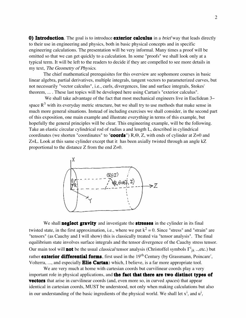
0) Introduction. The goal is to introduce exterior calculus in a brief way that leads directly to their use in engineering and physics, both in basic physical concepts and in specific engineering calculations. The presentation will be very informal. Many times a proof will be omitted so that we can get quickly to a calculation. In some "proofs" we shall look only at a typical term. It will be left to the readers to decide if they are compelled to see more details in my text, The Geometry of Physics. The chief mathematical prerequisites for this overview are sophomore courses in basic linear algebra, partial derivatives, multiple integrals, tangent vectors to parameterized curves, but not necessarily "vector calculus", i.e., curls, divergences, line and surface integrals, Stokes' theorem, ... . These last topics will be developed here using Cartan's "exterior calculus". We shall take advantage of the fact that most mechanical engineers live in Euclidean 3-space ®3 with its everyday metric structure, but we shall try to use methods that make sense in much more general situations. Instead of including exercises we shall consider, in the second part of this exposition, one main example and illustrate everything in terms of this example, but hopefully the general principles will be clear. This engineering example, will be the following. Take an elastic circular cylindrical rod of radius a and length L, described in cylindrical coordinates (we shorten "coordinates" to "coords") R,Θ, Z, with ends of cylinder at Z=0 and Z=L. Look at this same cylinder except that it has been axially twisted through an angle kZ proportional to the distance Z from the end Z=0.
We shall neglect gravity and investigate the stresses in the cylinder in its final twisted state, in the first approximation, i.e., where we put k2 = 0. Since "stress" and "strain" are "tensors" (as Cauchy and I will show) this is classically treated via "tensor analysis". The final equilibrium state involves surface integrals and the tensor divergence of the Cauchy stress tensor. Our main tool will not be the usual classical tensor analysis (Christoffel symbols ˝ijk ..,etc.) but rather exterior differential forms, first used in the 19th Century (by Grassmann, Poincareæ, Volterra, ..., and especially Elie Cartan) which, I believe, is a far more appropriate tool. We are very much at home with cartesian coords but curvilinear coords play a very important role in physical applications, and the fact that there are two distinct types of vectors that arise in curvilinear coords (and, even more so, in curved spaces) that appear identical in cartesian coords, MUST be understood, not only when making calculations but also in our understanding of the basic ingredients of the physical world. We shall let xi, and ui,
3
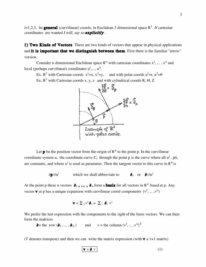
i=1,2,3, be general (curvilinear) coords, in Euclidean 3 dimensional space ®3. If cartesian coordinates are wanted I will, say so explicitly . 1) Two Kinds of Vectors. There are two kinds of vectors that appear in physical applications and it is important that we distinguish between them. First there is the familiar "arrow" version. Consider n dimensional Euclidean space ®n with cartesian coordinates x1, ... , xn and local (perhaps curvilinear) coordinates u1,..., un. Ex. ®2 with Cartesian coords x1=x, x2=y, and with polar coords u1=r, u2=œ Ex. ®3 with Cartesian coords x, y, z and with cylindrical coords R, Θ, Z
!
Let p be the position vector from the origin of ®n to the point p. In the curvilinear coordinate system u, the coordinate curve Ci through the point p is the curve where all uj , j≠i, are constants, and where ui is used as parameter. Then the tangent vector to this curve in ®n is $p/$ui which we shall abbreviate to $ i or $/$ui
At the point p these n vectors $1 , . .. , $n form a basis for all vectors in ®n based at p. Any vector v at p has a unique expansion with curvilinear coord components (v1, ... ,vn) v = Í i vi $ i = Í i $ i vi
We prefer the last expression with the components to the right of the basis vectors. We can then form the matrices $= the row ($1 , ... , $n ) and v = the column (v1, ... ,vn)T
! ! !
(T denotes transpose) and then we can write the matrix expression (with v a 1ª1 matrix) v = $ v (1)
4
(It is traditional to put the vectorial components in a column matrix, as we have.) Please beware though that in $ i vi or ($/$ui) vi or v = $ v , the bold $ does not differentiate the component term to the right; it is merely the symbol for a basis vector. Of course we can still differentiate a function f along a vector v by defining v(f) = ( Í i $ i vi )(f) = Í i $/$ui (f) vi := Í i ($ f/$ui ) vi replacing the basis vector $/$ui with bold $ by the partial differential operator $ /$ui and then applying to the function f. A vector is a first order differential operator on functions! In cylindrical coords R,Θ, Z in ®3 we have the basis vectors $R=$/$R, $œ =$/$Θ, and $Z =$/$Z. Let v be a vector at a point p. We can always find a curve u i=u i(t) through p whose veloci ty vector there is v, vi = dui/dt. Then if u' is a second coordinate system about p, we then have v' j = du'j/dt = ($u' j/$ui) dui/dt = ($u' j/$ui) vi. Thus the components of a vector transform under a change of coordinates by the rule v' j = Íi ($u' j/$ui) vi or as matrices v ' = ($u'/$u)v (2) where ($u'/$u) is the Jacobian matrix. This is the transformation law for the components of a contravariant vector, or tangent vector, or simply vector. There is a second, different type of vector. In linear algebra we learn that to each vector space V (in our case the space of all vectors at a point p) we can associate its dual vector space V* of all real linear functionals å: V‘® . In coordinates å(v) is a number å(v) = Íi aivi We shall explain why i is a subscript in ai shortly. The most familiar linear functional is the differential of a function df. As a function on vectors it is defined by the derivative of f along v df(v): =v(f) = Íi ($f/$ui) vi and so (df)i = $f/$ui Let us write df in a much more familiar form. In elementary calculus there is mumbo-jumbo to the effect that dui is a function of pairs of points: it gives you the difference in the ui coordinates between the points, and the points do not need to be close together. What is really meant is dui is the linear functional that reads off the i th component of any vector v with respect to the basis vectors of the coord system u dui (v) = dui (Íj $ j vj) := vi
Note that this agrees with dui (v) = v (ui) since v(ui) = (Íj $ j vj) (ui) = Íj ($ui/$uj) vj = Íj ∂ij vj = vi. Then we can write df(v) = Íi ($f/$ui) vi = Íi ($f/$ui) dui (v) i.e.,
5
df = Íi ($f/$ui) dui as usual, except that now both sides have meaning as linear functionals on vectors. Warning. We shall see that this is not the gradient vector of f! It is very easy to see that du1, ... , dun form a basis for the space of linear functionals at each point of the coordinate system u, since they are linearly independent. In fact, this basis of V* is the dual basis to the basis $1, ..., $n , meaning
dui ($ j ) = ∂ij Thus in the coordinate system u, every linear functional å is of the form å =Íi ai (u) dui where å($ j) =Íi ai (u) dui ($ j)= Íi ai (u)∂ij = aj
is the jth component of å. We shall see in section 8) that it is not true that every å is = df for some f! Corresponding to (1) we can write the matrix expansion for a linear functional as å = (a1 , ... , an) (du1 , ... , dun)T = a du (3) i.e., a is a row matrix and du is a column matrix! If V is the space of contravariant vectors at p, then V* is called the space of covariant vectors, or covectors, or 1-forms at p. Under a change of coordinates, using the chain rule, å = a'du' = a du = ( a) ( $u/$u' )(du') , and so
a' = a ($u/$u')= a ($u'/$u)-1 i.e., a'j = Íi ai ($ui/$u'j) (4)
which should be compared with (2). This is the law of transformation of components of a covector. Note that by definition, if å is a covector and v is a vector, then the value å(v) = a v =Íi ai vi is invariant, i.e., independent of the coordinates used. This also follows, from (2) and (4) å(v) = a' v' = a ($u/$u') ($u'/$u)v = a ($u'/$u)-1 ($u'/$u)v = a v Note that a vector can be considered as a linear functional on covectors, v(å) :=å(v) = Íi ai vi. 2) Superscripts, Subscripts, Summation Convention. First the "summation convent ion". Whenever we have a single term of an expression with any number of indices up and down, e.g., T abcde , if we rename one of the lower indices, say d so that it becomes the same as one of the upper indices, say b, and if we then sum over this index, the result, call it S,
6
Íb Tabcbe = Sace is called a contraction of T. The index b has disappeared (it was a summation or "dummy" index on the left expression; you could have called it anything.) This process of summing over a repeated index that occurs as both a subscript and a superscript occurs so often that we shall omit the summation sign and merely write, e.g., Tabcbe = Sace . This convention does not apply to two upper or two lower indices. Here is why. We have seen that if å is a covector, and if v is a vector then å(v) = ai vi is an invariant, independent of coordinates. But if we have another vector, say w =$w then Íi vi wi will not be invariant; Íi v'i w'i = v'T w' = [($u'/$u)v]T ($u'/$u) w =vT ($u'/$u)T ($u'/$u) w will not = vT w , for all v,w unless ($u'/$u)T= ($u'/$u)-1, i.e., unless the coordinate change matrix is an orthogonal matrix, as it is when u and u' are Cartesian coordinate systems. Our conventions regarding the components of vectors and covectors (contravariant¶ index up) and (covariant¶ index down) (*^) help us avoid errors! For example, in calculus, the differential equations for curves of steepest ascent for a function f are written in cartesian coords as dxi/dt = $f/$xi but these equations cannot be correct , say, in spherical coordinates, since we cannot equate the contravariant components vi of the velocity vector with the covariant components of the differential df; they transform in different ways under a (non-orthogonal) change of coordinates. We shall see the correct equations for this situation in section 3). Warning. Our convention (*^) applies only to the components of vectors and covectors. In å=aidxi, the ai are the components of a single covector å, while each individual dxi is itself a basis covector, not a component. The summation convention, however, always holds. I cringe when I see expressions like Íi vi wi in non-cartesian coords, for the notation is informing me that I have misunderstood the "variance" of one of the vectors. 3) Riemannian Metrics. One can identify vectors and covectors by introducing an additional structure, but the identification will depend on the structure chosen. The metric structure of ordinary Euclidean space ®3 is based on the fact that we can measure angles and lengths of vectors and scalar products < , >. The arc length of a curve C is ˆC ds where ds2 =dx2 +dy2 +dz2 in cartesian coords. In curvilinear coords u we have, putting dxk = ($xk/$ui) dui, and then ds2 =Ík (dxk)2 = Íi,j gij dui duj = gij dui duj (5) where
7
gij = Ík ($xk/$ui) ($xk/$uj) = (since the x coords are cartesian) <$p/$ui, $p/$uj> gij = <$ i , $ j> = gji and generally (6) <v,w> = gij vi wj
For example, consider the plane ®2 with cartesian coords x1 =x, x2=y, and polar coords u1=r, u2=œ. Then
!
gxx =1 gxy = 0
gyx = 0 gyy =1
"
# $
%
& ' i.e.,
!
gxx gxy
gyx gyy
"
# $
%
& ' =
!
1 0
0 1
"
# $
%
& '
Then, from x=r cosœ, dx = dr cosœ -r sinœ dœ, etc., we get ds2 = dr2 + r2 dœ2,
!
grr =1 gr" = 0
g"r = 0 g"" = r2
#
$ %
&
' ( i.e.,
!
grr gr"
g"r g#"
$
% &
'
( ) =
!
1 0
0 r2
"
# $
%
& ' (7)
which is "evident" from the picture
In spherical coords a picture shows ds2= dr2 + r2dÚ2 + r2 sin2Ú d…2, where Ú is co-latitude and … is - longitude, so (gij)= diag(1, r2, r2sin2Ú). In cylindrical coords, ds2=dR2+R2dΘ2+dZ2, with (gij) = diag ( 1, R2, 1). Let us look again at the expression (5). If å and ∫ are 1-forms, i.e., linear functionals, define their tensor product å·∫ to be the function of (ordered) pairs of vectors defined by å·∫ (v, w) :=å(v)∫(w) (8) In particular (dui · duk )(v, w) := vi wk Likewise ($ i · $ j) (å, ∫) = ai bj (why?) å·∫ is a bilinear function of v and w, i.e., it is linear in each when the other is unchanged. A second rank covariant tensor is just such a bilinear function and in the coord system u it can be expressed as Íi,j aij dui · duj
8
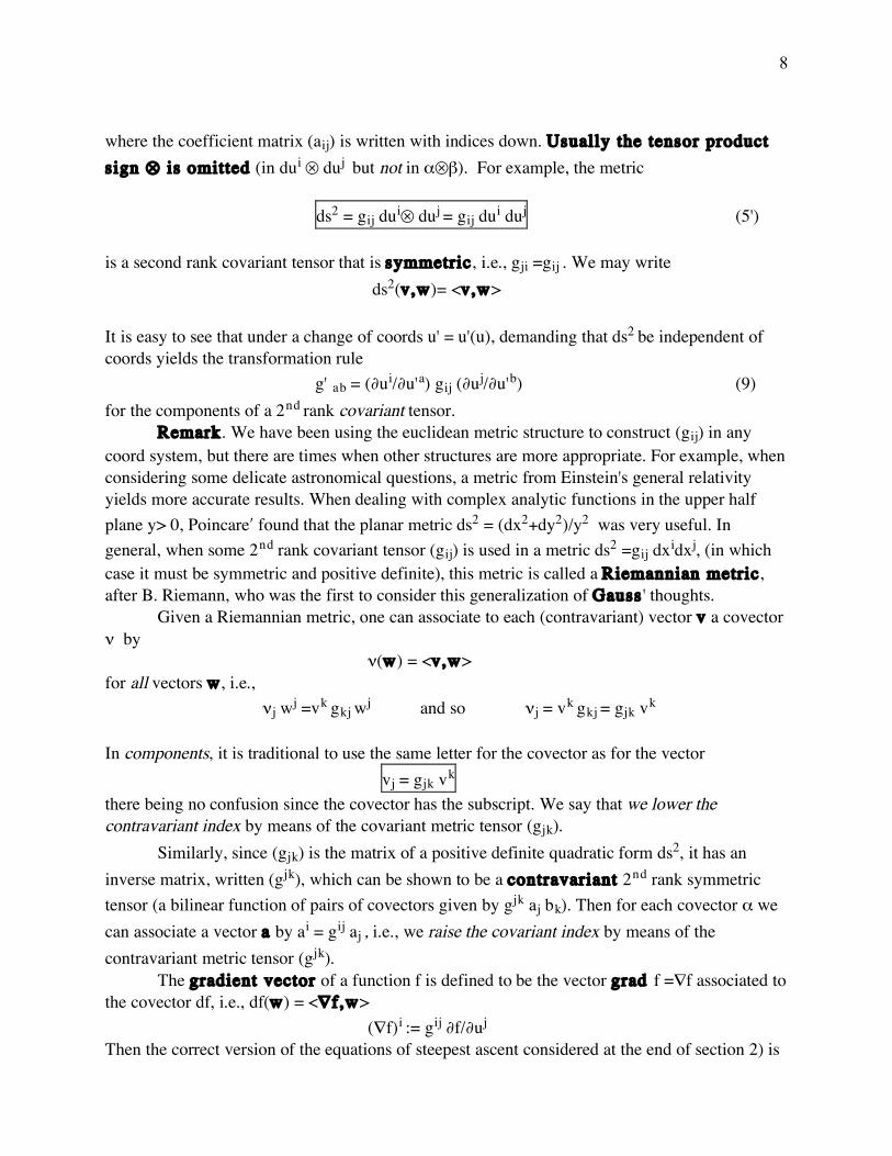
where the coefficient matrix (aij) is written with indices down. Usually the tensor product sign · is omitted (in dui · duj but not in å·∫). For example, the metric ds2 = gij dui· duj = gij dui duj (5') is a second rank covariant tensor that is symmetric, i.e., gji =gij . We may write ds2(v,w)= <v,w> It is easy to see that under a change of coords u' = u'(u), demanding that ds2 be independent of coords yields the transformation rule g' ab = ($ui/$u'a) gij ($uj/$u'b) (9) for the components of a 2nd rank covariant tensor. Remark. We have been using the euclidean metric structure to construct (gij) in any coord system, but there are times when other structures are more appropriate. For example, when considering some delicate astronomical questions, a metric from Einstein's general relativity yields more accurate results. When dealing with complex analytic functions in the upper half plane y> 0, Poincareæ found that the planar metric ds2 = (dx2+dy2)/y2 was very useful. In general, when some 2nd rank covariant tensor (gij) is used in a metric ds2 =gij dxidxj, (in which case it must be symmetric and positive definite), this metric is called a Riemannian metric, after B. Riemann, who was the first to consider this generalization of Gauss ' thoughts. Given a Riemannian metric, one can associate to each (contravariant) vector v a covector ¥ by ¥(w) = <v,w> for all vectors w, i.e., ¥j wj =vk gkj wj and so ¥j = vk gkj = gjk vk In components, it is traditional to use the same letter for the covector as for the vector vj = gjk vk there being no confusion since the covector has the subscript. We say that we lower the contravariant index by means of the covariant metric tensor (gjk). Similarly, since (gjk) is the matrix of a positive definite quadratic form ds2, it has an inverse matrix, written (gjk), which can be shown to be a contravariant 2nd rank symmetric tensor (a bilinear function of pairs of covectors given by gjk aj bk). Then for each covector å we can associate a vector a by ai = gij aj , i.e., we raise the covariant index by means of the contravariant metric tensor (gjk). The gradient vector of a function f is defined to be the vector grad f =#f associated to the covector df, i.e., df(w) = <#f,w> (#f)i := gij $f/$uj Then the correct version of the equations of steepest ascent considered at the end of section 2) is
9
dui/dt = (#f)i = gij $f/$uj in any coords. For example, in polar coords, from (7), we see grr=1, gœœ =1/r2 , grœ= 0 =gœr. 4) Tensors. We shall consider examples rather than generalities. (i) A tensor of the 3rd rank, twice contravariant, once covariant, is locally of the form A = $ i ·$ j Aijk · duk It is a trilinear function of pairs of covectors å = ai dui, ∫= bjduj, and a single vector v= $k vk A(å, ∫, v) = ai bj Aijk vk summed, of course, on all indices. It's components transform as A' efg = ($u'e/$ui) ($u'f/$uj) Aijk ($uk/$u'g) If we contract on i and k, the result Bj := Aiji are the components of a contravariant vector B'f = A'efe = Aijk($u'f/$uj)($uk/$u'e)($u'e/$ui) = Aijk ($u'f/$uj) ∂ki = Aiji ($u'f/$uj) = ($u'f/$uj) Bj.
(ii) A linear transformation is a 2nd rank ("mixed") tensor P= $ iPij · duj. Rather than thinking of this as a real valued bilinear function of a covector and a vector, we usually consider it as a linear function taking vectors into vectors, (called a vector valued 1-form in 13)) P(v) = [$ iPij · duj] (v) := $ i Pij {duj(v)} = $ i Pij vj
i.e., the usual [P(v)]i = Pij vj
Under a change of coords the matrix (Pij) transforms as P' = ($u'/$u) P ($u'/$u)-1, as usual. If we contract we obtain a scalar (invariant), tr P := Pii , the trace of P. tr P' = tr P ($u'/$u)-1($u'/$u) = tr P
Beware. If we have a twice covariant tensor G (a "bilinear form"), e.g., a metric (gij), then Ík gkk is not a scalar, although it is the trace of the matrix; see e.g., equation (7). This is because the transformation law for the matrix G is, from (9), G'= ($u/$u')T G ($u/$u') and tr G' ≠ tr G generically.
INTEGRALS and EXTERIOR FORMS
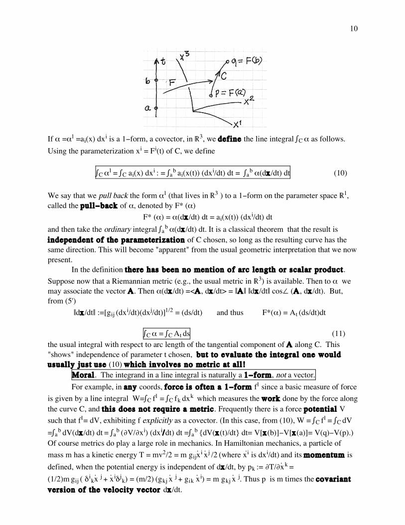
5) Line Integrals. We illustrate in ®3 with any coords x. For simplicity, let C be a smooth "oriented" or "directed" curve, the image under F :[a,b]™ ®1‘C ™ ®3 , (which is read " F maps the interval [a,b] on ®1 into the curve C in ®3") with F(a)= some p and F(b) = some q.
10
If å =å1 =ai(x) dxi is a 1-form, a covector, in ®3, we define the line integral ˆC å as follows. Using the parameterization xi = Fi(t) of C, we define ˆC å1 = ˆC ai(x) dxi : = ˆab ai(x(t)) (dxi/dt) dt = ˆab å(dx/dt) dt (10) We say that we pull back the form å1 (that lives in ®3 ) to a 1-form on the parameter space ®1, called the pull-back of å, denoted by F* (å) F* (å) = å(dx/dt) dt = ai(x(t)) (dxi/dt) dt and then take the ordinary integral ˆab å(dx/dt) dt. It is a classical theorem that the result is independent of the parameterization of C chosen, so long as the resulting curve has the same direction. This will become "apparent" from the usual geometric interpretation that we now present. In the definition there has been no mention of arc length or scalar product. Suppose now that a Riemannian metric (e.g., the usual metric in ®3) is available. Then to å we may associate the vector A. Then å(dx/dt) =<A, dx/dt> = ˜A˜ ˜dx/dt˜ cos‚ (A, dx/dt). But, from (5') ˜dx/dt˜ :=[gij (dxi/dt)(dxj/dt)]1/2 = (ds/dt) and thus F*(å) = At (ds/dt)dt ˆC å = ˆC At ds (11) the usual integral with respect to arc length of the tangential component of A along C. This "shows" independence of parameter t chosen, but to evaluate the integral one would usually just use (10) which involves no metric at all! Moral. The integrand in a line integral is naturally a 1-form, not a vector. For example, in any coords, force is often a 1-form f1 since a basic measure of force is given by a line integral W=ˆC f1 = ˆC fk dxk which measures the work done by the force along the curve C, and this does not require a metric. Frequently there is a force potential V such that f1= dV, exhibiting f explicitly as a covector. (In this case, from (10), W = ˆC f1 = ˆC dV =ˆab dV(dx/dt) dt = ˆab ($V/$xi) (dxi/dt) dt =ˆab {dV(x(t)/dt} dt= V[x(b)]-V[x(a)]= V(q)-V(p).) Of course metrics do play a large role in mechanics. In Hamiltonian mechanics, a particle of mass m has a kinetic energy T = mv2/2 = m gijx‹i x‹j /2 (where xi‹ is dxi/dt) and its momentum is defined, when the potential energy is independent of dx/dt, by pk := $T/$x‹k = (1/2)m gij ( ∂ikx‹ j + x‹i∂jk) = (m/2) (gkj x‹ j + gik x‹i) = m gkj x‹ j. Thus p is m times the covariant version of the velocity vector dx/dt.
11
The momentum 1-form "pi dxi " on the "phase space" with coords (x, p) plays a central role in all of Hamiltonian mechanics.
6) Exterior 2-Forms.We have already defined the tensor product å1·∫1 of two 1-forms to be the bilinear form å1·∫1(v,w) =å1(v)∫1(w). We now define a more geometrically significant wedge or exterior product å°∫ to be the skew symmetric bilinear form
å1°∫1 := å1·∫1- ∫1· å1
duj°duk (v,w) = vjwk -vkwj =
!
duj(v) du
j(w)
duk(v) du
k(w)
(12)
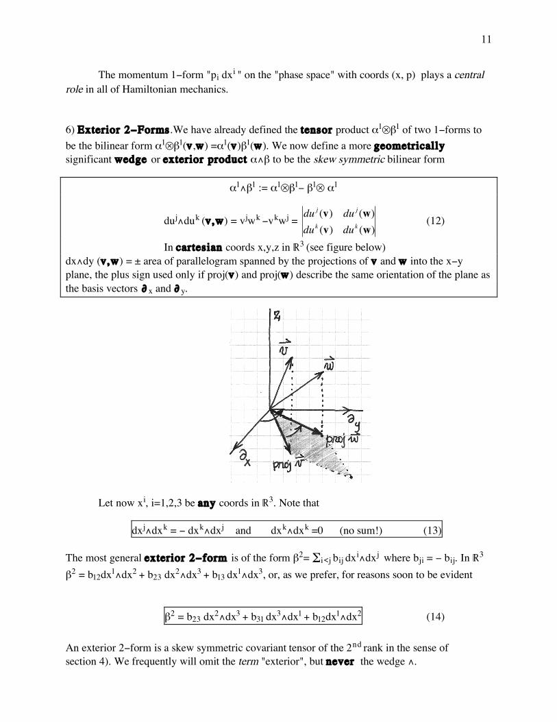
In cartesian coords x,y,z in ®3 (see figure below) dx°dy (v,w) = ± area of parallelogram spanned by the projections of v and w into the x-y plane, the plus sign used only if proj(v) and proj(w) describe the same orientation of the plane as the basis vectors $x and $y.
Let now xi, i=1,2,3 be any coords in ®3. Note that
dxj°dxk = - dxk°dxj and dxk°dxk =0 (no sum!) (13)
The most general exterior 2-form is of the form ∫2= Íi<j bij dxi°dxj where bji = - bij. In ®3
∫2 = b12dx1°dx2 + b23 dx2°dx3 + b13 dx1°dx3, or, as we prefer, for reasons soon to be evident
∫2 = b23 dx2°dx3 + b31 dx3°dx1 + b12dx1°dx2 (14) An exterior 2-form is a skew symmetric covariant tensor of the 2nd rank in the sense of section 4). We frequently will omit the term "exterior", but never the wedge °.
12
(7) Exterior p-Forms and Algebra in ®n. The exterior algebra has the following properties.We have already discussed 1-forms and 2-forms. An (exterior) p-form åp in ®n is a completely skew symmetric multilinear function of p-tuples of vectors å(v1, ... , vp ) that changes sign whenever two vectors are interchanged. In any coords x, e.g., the 3-form dxi ° dxj °dxk in ®n is defined by
By counting the number of interchanges of pairs of dx's one can see the commutation rule
åp°∫q =(-1)pq ∫q°åp (16)
8) The Exterior Differential d. First a remark. If v = $a va is a contravariant vectorfield, then generically ($va/$xb) = Qab do not yield the components of a tensor in curvilinear coords, as is easily seen from looking at the transformation of Q under a change of coords and using (2). It is, however, always possible, in ®n and in any coords, to take a very important "exterior"derivative d of p-forms. We define dåp to be a p+1 form, as follows; å is a sum of forms of the type a(x) dxi ° dxj ° ...°dxk. Define
In cartesian coords we then have correspondences with vector analysis
df0 & #f Âdx då1& ( curl a)Â"dA" d∫2 & div B "dvol" (19
the quotes, e.g., "dA" being used since this is not really the differential of a 1-form. We shall make this correspondence precise, in any coordinates, later. Exterior differentiation of exterior forms does essentially grad, curl and divergence with a single general formula (17)!! Also, this machinery works in ®n as well. Furthermore, d does not require a metric. On the other hand,
14
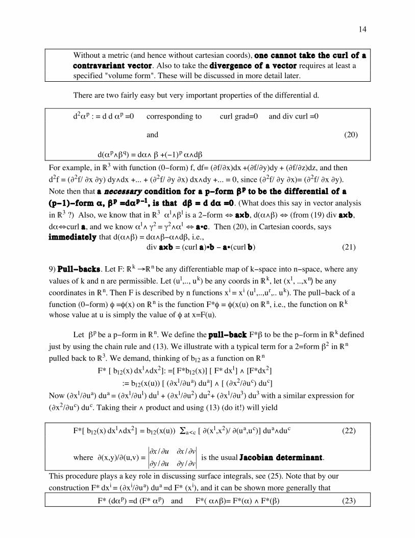
Without a metric (and hence without cartesian coords), one cannot take the curl of a contravariant vector. Also to take the divergence of a vector requires at least a specified "volume form". These will be discussed in more detail later.
There are two fairly easy but very important properties of the differential d.
d2åp : = d d åp =0 corresponding to curl grad=0 and div curl =0
Let ∫p be a p-form in ®n. We define the pull-back F*∫ to be the p-form in ®k defined just by using the chain rule and (13). We illustrate with a typical term for a 2=form ∫2 in ®n pulled back to ®3. We demand, thinking of b12 as a function on ®n
F* [ b12(x) dx1°dx2]: =[ F*b12(x)] [ F* dx1] ° [F*dx2] := b12(x(u)) [ ($x1/$ua) dua] ° [ ($x2/$uc) duc] Now ($x1/$ua) dua = ($x1/$u1) du1 + ($x1/$u2) du2+ ($x1/$u3) du3 with a similar expression for ($x2/$uc) duc. Taking their ° product and using (13) (do it!) will yield
This procedure plays a key role in discussing surface integrals, see (25). Note that by our construction F* dxi = ($xi/$ua) dua =d F* (xi), and it can be shown more generally that
(20) and (23) are what make forms so powerful and useful, compared to vector fields. In general, and for our example of F:®2 ‘ ®3, we can define the push forward F§ of a vector at a single point u, e.g., F§ $/$ua : = Íi ($xi/$ua) $/$xi , yielding a vector at F(u), but we can't map the vectorfield $/$ua into a vectorfield in ®3 if, e.g., there are distinct points u and u' such that F(u) =F(u'), because generically the two resulting push forwards, one from u and one from u', won't agree at the image point. Also if the image space dimension n is greater than that of the source space k, then the push forward vectors will not be defined on all of ®n. However, the pull-back of a p-form field is always a p-form field. The geometric meaning of the push forward F§ v is the following. At a point u the vector v(u) is the velocity vector to some curve C through u, v= du/dt. Then F§ v is the velocity vector to the image curve F(C), dx(u(t))/dt = ($x/$u) du/dt, i.e., dxi/dt = ($xi/$ua) dua/dt. It is a fact that F*åp (v, . . .w) = åp( F§v,..., F §w) (24) which supplies the geometric meaning of the pull-back F*, namely, the pull-back of å, applied to a p-tuple of vectors at u, has the same value as the original form å on the push forward of these vectors to F(u). In fact, using (24) we can define the pullback of any covariant tensor of rank p, not just p-forms. In particular, as we shall see, the pull back of the metric tensor is the principal ingredient of the "strain tensor" in elasticity.
Note that when F: ®n ‘®n is the identity map, using two sets of coordinates, e.g., x= r cosœ, y= r sinœ, then the pull-back F*å is simply expressing the form å ,given in coords x, in terms of the new coords u. 10) Surface Integrals and "Stokes ' theorem". We illustrate with a surface V2 in ®3. Assume, e.g., that ®3 has the "right handed orientation". Assume that V2 is also "oriented" meaning that at each point p of V there is a preferred sense of rotation of the tangent plane at p, (indicated in the figure below by a circular arrow), and this sense varies continuously on V. For example, if V has a continuous choice of normal vector everywhere ( unlike a MoÜbius band) then the right hand rule for ®3 will yield an orientation for V. We are going to define ˆV ∫2 for any 2-form ∫. If V is sufficiently small we may choose a parameterization of V that yields the same orientation as V, i.e., we ask for a smooth 1-1 map F : region S2 ™ some ®2 ‘ onto V2 ™ ®3 xi =xi(t1,t2) (If V is too large for such a parameterization, break it up into smaller pieces and add up the individual resulting integrals.) We picture the resulting t1, t2 coordinate curves on V as engraved on V just as latitude and longitude curves are engraved on globes of the Earth. We demand that the sense of rotation from the engraved t1 curve to the t2 curve on V (i.e, from F§ $1 to F§$2) is the same as the given orientation arrow on V. We say V=F(S).
reducing the problem to defining the integral of the pull-back of ∫ over S. First write this out, but for simplicity we just look at the term b31(x) dx3°dx1 . From (22)
= ˆS b31(x(t))[ $(x3,x1)/ $(t1,t2)]dt1°dt2 := ˆS b31(x(t))[ $(x3,x1)/ $(t1,t2)]dt1dt2 and where the very last integral, with no °, is the usual double integral over a region S in the t1t2 plane. Thus
ˆV ∫2 = ˆF(S) ∫2 =ˆS F*∫2 (25) := ˆS{b23(x(t))[$(x2,x3)/$(t1,t2)] +b31(x(t))[$(x3,x1)/$(t1,t2)] +b12(x(t)) [$(x1,x2)/$(t1,t2)]} dt1dt2 Note that one needn't remember this. One merely uses the chain rule in calculus and dt1°dt2 =-dt2°dt1 to get an integral over a region in the t1 , t2 plane, then omit the ° and evaluate the resulting double integral. Interpretation. In cartesian coords with the usual metric in ®3, associate to ∫2 the vector B =( B1=b23, B2=b31, B3=b12)T. n= [$x/$t1]ª [$x/$t2] is a normal to the surface with components ([$(x2,x3)/$(t1,t2)], [$(x3,x1)/$(t1,t2)], [$(x1,x2)/$(t1,t2)])T.
17
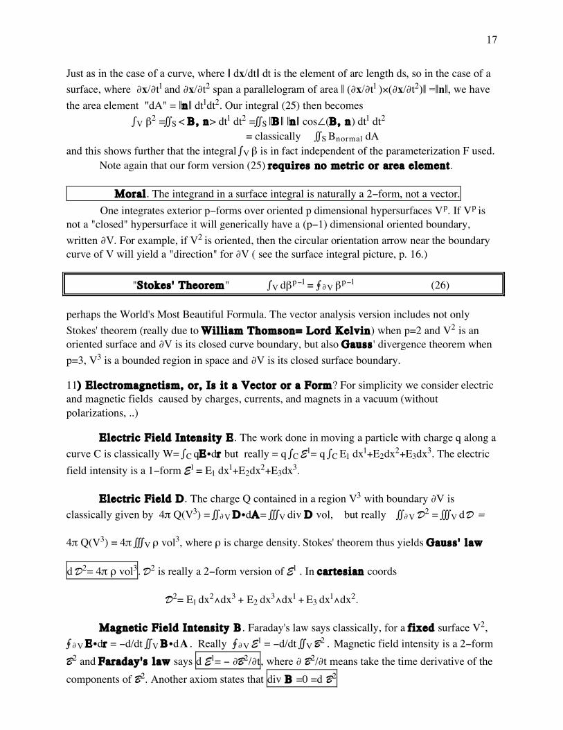
Just as in the case of a curve, where ˜ dx/dt˜ dt is the element of arc length ds, so in the case of a surface, where $x/$t1 and $x/$t2 span a parallelogram of area ˜ ($x/$t1 )ª($x/$t2)˜ =˜n˜, we have the area element "dA" = ˜n˜ dt1dt2. Our integral (25) then becomes ˆV ∫2 =ˆˆS < B, n> dt1 dt2 =ˆˆS ˜B˜ ˜n˜ cos‚(B, n) dt1 dt2 = classically ˆˆS Bnormal dA and this shows further that the integral ˆV ∫ is in fact independent of the parameterization F used. Note again that our form version (25) requires no metric or area element. Moral. The integrand in a surface integral is naturally a 2-form, not a vector. One integrates exterior p-forms over oriented p dimensional hypersurfaces Vp. If Vp is not a "closed" hypersurface it will generically have a (p-1) dimensional oriented boundary, written $V. For example, if V2 is oriented, then the circular orientation arrow near the boundary curve of V will yield a "direction" for $V ( see the surface integral picture, p. 16.)
"Stokes ' Theorem" ˆV d∫p-1 = ¨$V ∫p-1 (26)
perhaps the World's Most Beautiful Formula. The vector analysis version includes not only Stokes' theorem (really due to William Thomson= Lord Kelvin) when p=2 and V2 is an oriented surface and $V is its closed curve boundary, but also Gauss ' divergence theorem when p=3, V3 is a bounded region in space and $V is its closed surface boundary.
11) Electromagnetism, or, Is it a Vector or a Form? For simplicity we consider electric and magnetic fields caused by charges, currents, and magnets in a vacuum (without polarizations, ..)
Electric Field Intensity E. The work done in moving a particle with charge q along a curve C is classically W= ˆC qEÂdr but really = q ˆC E1= q ˆC E1 dx1+E2dx2+E3dx3. The electric field intensity is a 1-form E1 = E1 dx1+E2dx2+E3dx3.
Electric Field D. The charge Q contained in a region V3 with boundary $V is classically given by 4π Q(V3) = ˆˆ$V DÂdA= ˆˆˆV div D vol, but really ˆˆ$V D2 = ˆˆˆV d D =
4π Q(V3) = 4π ˆˆˆV ‰ vol3, where ‰ is charge density. Stokes' theorem thus yields Gauss ' law
d D2= 4π ‰ vol3. D2 is really a 2-form version of E1 . In cartesian coords
D2= E1 dx2°dx3 + E2 dx3°dx1 + E3 dx1°dx2.
Magnetic Field Intensity B. Faraday's law says classically, for a fixed surface V2, ¨$V EÂdr = -d/dt ˆˆV BÂd
!
A . Really ¨$V E1 = -d/dt ˆˆV B2 . Magnetic field intensity is a 2-form
B2 and Faraday's law says d E1= - $B2/$t, where $ B2/$t means take the time derivative of the
components of B2. Another axiom states that div B =0 =d B2
18
Magnetic Field H. Ampere-Maxwell says classically
¨C=$V HÂdr= 4πˆˆVjÂdA+ d/dt ˆˆV DÂdA where V2 is fixed and j is the current vector. Really ¨C=$V H1= 4πˆˆV j 2+ d/dt ˆˆV D2
and thus d H 1= 4π j 2+ $D2/$t, where j 2 = the current 2-form whose integral over V2 (with a
preferred normal direction), measures the time rate of charge passing through V2 in that direction. H 1 is a 1-form version of B2. In cartesian coords H 1= B23dx1 + B31dx2+ B12dx3.
Heaviside-Lorentz Force. Classically the electromagnetic force acting on a particle of charge q moving with velocity v is given by f = q(E + vªB). We have seen that force and the electric field should be 1-forms, f 1= q(E1 + ??). v is definitely a vector, and B is a 2-form! We now discuss this dilemma raised by the vector product ª and its resolution will play a large role in our discussion of elasticity also.
12) Interior Products. We are at home with the fact å1°∫1 is a 2-form replacement for a ª product of vectors in ®3 , but if we had started out with two vectors A and B it would require a metric to change them to 1-forms. It turns out there is also a 1-form replacement that is frequently more useful, and will resolve the Lorentz force problem.
In ®n, if v is a vector and ∫p is a p-form, p>0, we define the interior product of v and ∫ to be the (p-1)-form iv∫ (sometimes we write i(v) ∫) with values
iv∫p (A2 , ,, Ap) := ∫p(v, A2 , , , Ap) (27)
(It can be shown that this is a contraction, (iv∫)bc... = vi ∫ibc...)
This is a form since it clearly is multilinear in A2 , . . Ap , since ∫ is, and changes sign under each interchange of the A's, and is defined independent of any coords. In the case of a 1-form ∫, iv∫ is the 0-form (function)
iv∫1= ∫1(v) = the function bi vi which = <v, b> in any Riemannian metric.
Look at iv(å1°∫1). iv(å1°∫1)(C) =(å1°∫1)(v,C)= å(v)∫(C) -å(C)∫(v)
= (ivå) ∫(C) - [å iv∫](C) = [(ivå) ∫ - (iv∫)å](C)
A more gruesome calculation shows the general product rule iv (åp°∫q) = [iv(åp)]°∫q +(-1)påp °[iv ∫q] (28) just as for the differential d.
19
13)Volume Forms and Cartan's Vector Valued Exterior Forms. Let x,y be positively oriented Cartesian coords in ®2. The area 2-form in the cartesian plane is vol2 = dx°dy, but in polar coords we have vol2= r dr°dœ. Looking at (7) we note that r= √g, where g := det (gij) (29) In any Riemannian metric, in any oriented ®n, we define the volume n-form to be voln := √gdx1°...°dxn (30) in any positively oriented curvilinear coords. It can be shown that this is indeed an n-form (modulo some question of orientation that I do not wish to consider here.) In spherical coords in ®3 we get, since (gij) = diag (1, r2, r2sin2 œ) the familiar vol3= r2 sinœ dr°dœ°dƒ. Note now the following in ®3 in any coords. For any vector v iv vol3 = iv √g dx1°dx2°dx3 = √g iv( dx1°dx2°dx3) Now apply the product rule (28) repeatedly iv( dx1°dx2°dx3)= v1 dx2°dx3 - dx1 °iv (dx2°dx3) = v1 dx2°dx3 - dx1 °[v2 dx3- v3 dx2] = v1 dx2°dx3 - v2 dx1°dx3 + v3 dx1°dx2 and so
Remark. For a surface V2 in Riemannian ®3, with unit normal vector field n, it is easy to see that in vol3 is the area 2-form for V2 . Simply look at its value on a pair of vectors A, B tangent to V; in vol3(A,B) =vol3(n, A,B)= area spanned by A and B. Comparing (31) with (14) we see that the most general 2-form ¥2 in ®3, in any coords, is of the form iv vol3 where v1 = ¥23 /√g , etc. In electromagnetism, D2= iEvol3. The same procedure works for an (n-1) form in ®n. Note that this does not require an entire metric tensor; we use only the volume element. If we have a distinguished volume form (i.e., if we have the notion of the volume spanned by a "positively oriented" n-tuple of vectors in ®n), even if it is not derived from a metric, we shall use the same notation in positively oriented coords where √g is now merely a fixed given coefficient. (Warning, this notation is not standard.) voln = √g dx1° ...°dxn If we have a volume form, we can define the divergence of a vector field v as follows (div v) voln : = d iv voln = d √g [v1 dx2°dx3°...°dxn - v2 dx1°dx3... dxn + ...]
= [$(v1√g)/$x1 + $(v2√g)/$x2 +...] dx1° ...°dxn i.e., div v = (1/√g) $/$xi (√g vi) (32) If, furthermore, the volume form comes from a Riemannian metric we can define the Laplacian of a function f by
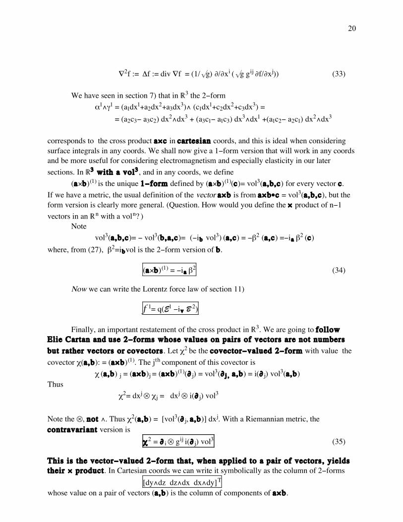
corresponds to the cross product aªc in cartesian coords, and this is ideal when considering surface integrals in any coords. We shall now give a 1-form version that will work in any coords and be more useful for considering electromagnetism and especially elasticity in our later sections. In ®3 with a vol3 , and in any coords, we define (aªb)(1) is the unique 1-form defined by (aªb)(1)(c)= vol3(a,b,c) for every vector c. If we have a metric, the usual definition of the vector aªb is from aªbÂc = vol3(a,b,c), but the form version is clearly more general. (Question. How would you define the ª product of n-1 vectors in an ®n with a voln? ) Note vol3(a,b,c)= - vol3(b,a,c)= (-ib vol3) (a,c) = -∫2 (a,c) =-ia ∫2 (c) where, from (27), ∫2=ibvol is the 2-form version of b.
(aªb)(1) = -ia ∫2 (34)
Now we can write the Lorentz force law of section 11)
f 1= q(E1 -iv B 2)
Finally, an important restatement of the cross product in ®3. We are going to follow Elie Cartan and use 2-forms whose values on pairs of vectors are not numbers but rather vectors or covectors. Let ⋲2 be the covector-valued 2-form with value the covector ⋲(a,b): = (aªb)(1). The jth component of this covector is ⋲ (a,b) j = (aªb)j = (aªb)(1)($ j) = vol3($j , a,b) = i($ j) vol3(a,b) Thus ⋲2= dxj · ⋲j = dxj · i($ j) vol3
Note the ·, not °. Thus ⋲2(a,b) = [vol3($ j, a,b)] dxj. With a Riemannian metric, the contravariant version is ⋲2 = $ i · gij i($ j) vol3 (35)
This is the vector-valued 2-form that, when applied to a pair of vectors, yields their ª product. In Cartesian coords we can write it symbolically as the column of 2-forms [dy°dz dz°dx dx°dy]T whose value on a pair of vectors (a,b) is the column of components of aªb.
21
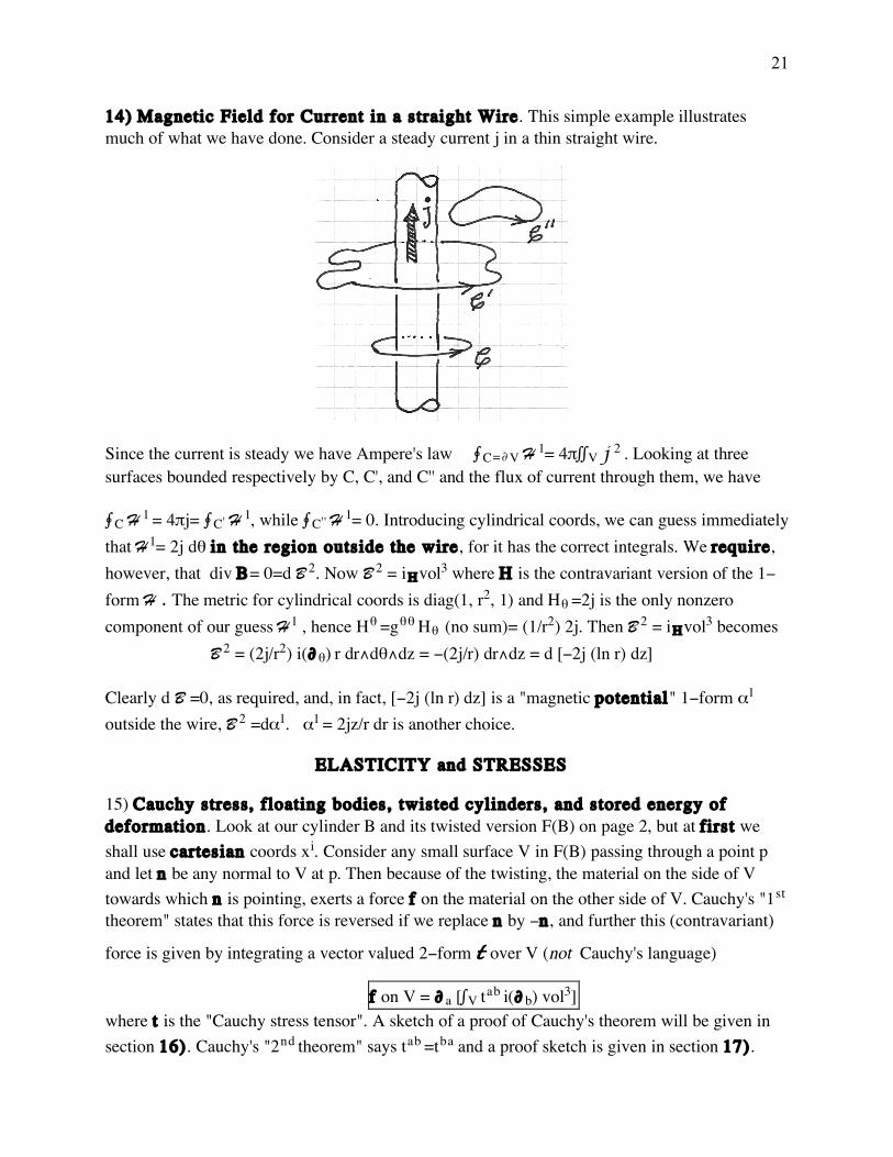
14) Magnetic Field for Current in a straight Wire. This simple example illustrates much of what we have done. Consider a steady current j in a thin straight wire.
Since the current is steady we have Ampere's law ¨C=$V H 1= 4πˆˆV j 2 . Looking at three surfaces bounded respectively by C, C', and C'' and the flux of current through them, we have
¨C H 1 = 4πj= ¨C' H 1, while ¨C'' H 1= 0. Introducing cylindrical coords, we can guess immediately that H 1= 2j dœ in the region outside the wire, for it has the correct integrals. We require, however, that div B= 0=d B 2. Now B 2 = iHvol3 where H is the contravariant version of the 1-form H . The metric for cylindrical coords is diag(1, r2, 1) and Hœ =2j is the only nonzero component of our guess H 1 , hence Hœ =gœœ Hœ (no sum)= (1/r2) 2j. Then B 2 = iHvol3 becomes B 2 = (2j/r2) i($œ) r dr°dœ°dz = -(2j/r) dr°dz = d [-2j (ln r) dz]
Clearly d B =0, as required, and, in fact, [-2j (ln r) dz] is a "magnetic potential" 1-form å1 outside the wire, B 2 =då1. å1 = 2jz/r dr is another choice.
ELASTICITY and STRESSES
15) Cauchy stress, floating bodies, twisted cylinders, and stored energy of deformation. Look at our cylinder B and its twisted version F(B) on page 2, but at first we shall use cartesian coords xi. Consider any small surface V in F(B) passing through a point p and let n be any normal to V at p. Then because of the twisting, the material on the side of V towards which n is pointing, exerts a force f on the material on the other side of V. Cauchy's "1st theorem" states that this force is reversed if we replace n by -n, and further this (contravariant)
force is given by integrating a vector valued 2-form t over V (not Cauchy's language)
f on V = $a [ˆV tab i($b) vol3] where t is the "Cauchy stress tensor". A sketch of a proof of Cauchy's theorem will be given in section 16). Cauchy's "2nd theorem" says tab =tba and a proof sketch is given in section 17).
22
As a warm-up check of our machinery, let us look first at an example of the simplest type of stress from elementary physics. In the case of a non-viscous fluid, given a very small parallelogram spanned by v and w and normal n=vªw, the fluid on the side to which n is pointing exerts a force on the other side approximated by - p vªw, where p is the hydrostatic
pressure. From (35) the stress vector valued 2-form is given by t = -$ i · p gij i($ j) vol3.
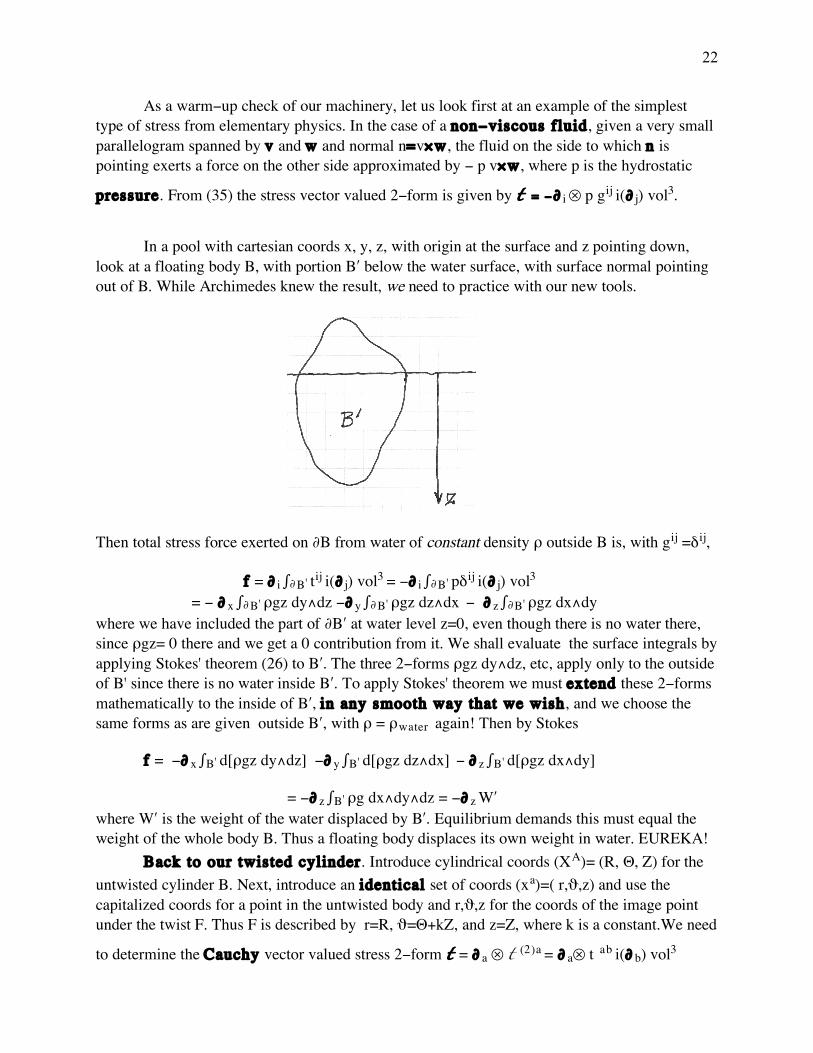
In a pool with cartesian coords x, y, z, with origin at the surface and z pointing down, look at a floating body B, with portion Bæ below the water surface, with surface normal pointing out of B. While Archimedes knew the result, we need to practice with our new tools.
Then total stress force exerted on $B from water of constant density ‰ outside B is, with gij =∂ij,
f = $ i ˆ$B' tij i($ j) vol3 = -$ i ˆ$B' p∂ij i($ j) vol3 = - $x ˆ$B' ‰gz dy°dz -$y ˆ$B' ‰gz dz°dx - $z ˆ$B' ‰gz dx°dy where we have included the part of $Bæ at water level z=0, even though there is no water there, since ‰gz= 0 there and we get a 0 contribution from it. We shall evaluate the surface integrals by applying Stokes' theorem (26) to Bæ. The three 2-forms ‰gz dy°dz, etc, apply only to the outside of B' since there is no water inside Bæ. To apply Stokes' theorem we must extend these 2-forms mathematically to the inside of Bæ, in any smooth way that we wish, and we choose the same forms as are given outside Bæ, with ‰ = ‰water again! Then by Stokes
= -$z ˆB' ‰g dx°dy°dz = -$z Wæ where Wæ is the weight of the water displaced by Bæ. Equilibrium demands this must equal the weight of the whole body B. Thus a floating body displaces its own weight in water. EUREKA! Back to our twisted cylinder. Introduce cylindrical coords (XA)= (R, Θ, Z) for the untwisted cylinder B. Next, introduce an identical set of coords (xa)=( r,Ú,z) and use the capitalized coords for a point in the untwisted body and r,Ú,z for the coords of the image point under the twist F. Thus F is described by r=R, Ú=Θ+kZ, and z=Z, where k is a constant.We need
to determine the Cauchy vector valued stress 2-form t = $a · t (2)a = $a· t ab i($b) vol3
23
on F(B) in terms of the twisting forces and the material from which B is made. We shall do this by first pulling this 2-form back to the untwisted body B by the following procedure; we pull
back the 2-forms t (2)a by F* and we push the vectors $a back to B by the inverse (F-1)§, which
exists since F is a 1-1 deformation. The resulting vector valued 2-form on B is of the form
S = (F-1)§($a) · F*t (2)a = (F-1)§($a) · F* [ t ab i($b) vol3]
(36)
S= $A · S(2)A = $A · SAB i($B) VOL3
called the "2nd Piola-Kirchhoff " vector valued stress 2-form. We shall relate this form to the twist F by a generalization of Hooke's law.
We need to know how this twist F has stretched, sheared, rotated, ... the body, and this is described as follows. The euclidean metric is dS2= (dR2+R2dΘ2+ dZ2) = ds2= (dr2+r2dÚ2 +dz2). The pull back (section 9), last paragarph) of ds2 under the twist F is given by the chain rule
= dR2 +R2[dΘ+ kdZ]2 +dZ2 = dR2+ R2[dΘ2 +2k dΘdZ +k2dZ2] +dZ2 Recall what this is saying. At a point R, Θ,Z of the untwisted body, given two vectors A,B, we have not only the scalar product < A, B> =dS2 (A,B) but also the scalar product of the images after the twist, i.e., from (24), ds2 ( F§A,F§B) =: (F*ds2)(A,B). Then one measure of how much the twist F is distorting distances and angles is defined by the Lagrange deformation tensor E := (½)[F* ds2-dS2] (37) The quadratic form (covariant second rank tensor) E is determined by its square matrix. How do the stresses depend on the deformations? In our twisting case we have E= kR2dΘdZ + ½ k2R2dZ2. We will work only to the first approximation for small k, i.e., we shall put k2 =0, so E=kR2 dΘdZ = ½ kR2 (dΘdZ + dZ dΘ). We write the components as a symmetric matrix
(EIJ) =
!
0 0 0
0 0 kR2/ 2
0 kR2/ 2 0
"
#
$ $ $
%
&
' ' '
The mixed version, using EAB = GAI EIB and (GKL)=diag(1, 1/R2, 1), is the (non-symmetric)
24
(EAB) =
!
0 0 0
0 0 k / 2
0 kR2/ 2 0
"
#
$ $ $
%
&
' ' '
and thus tr E = EAA=0 "mod k2", i.e., putting k2=0. Finally, putting EAB = EAI GIB
(EAB) =
!
0 0 0
0 0 k / 2
0 k / 2 0
"
#
$ $ $
%
&
' ' '
"Linear elasticity" assumes a linear, vastly generalized "Hookes law" relating the stress S to the deformation E. Assuming the body is "isotropic" ( i.e., the material has no special internal directional structure such as grains in wood), it can then be shown (e.g., [TF, equation (D.9)] that there are then only 2 "elastic constants" µ and ¬ relating S to E
SAB = 2µ EAB + ¬ (tr E) GAB (38)
and so
(SAB ) =
!
0 0 0
0 0 µk
0 µk 0
"
#
$ $ $
%
&
' ' '
This gives rise to the 2nd Piola-Kirchhoff vector valued stress 2-form on the undeformed body
To get correct "dimensions" for force we use the "physical" components of force, i.e., we normalize the basis vectors. Since grr =1= gzz , $r and $z are unit vectors, call them er and ez. But gÚÚ =r2, and so $Ú, by (6), has length r, and so we put eÚ = r-1 $Ú. We make no changes to the form parts dr, dÚ, and dz.
t 2= µkr2 eÚ · dr°dÚ + µkr ez · dz°dr (40)
We shall now see the consequences of this Cauchy stress. Look first at the lateral surface
r=a. Then dr=0 there and so t =0 on this surface. This means that no external "traction"
on this part of the boundary is needed for this twisting.
Now look at the end boundary at z=L. From (40) we have stress from outside
µkr2 eÚ · dr°dÚ
acting in the eÚ direction. This has to be supplied by external tractions since there is no part of the body past its end. What is the moment of the traction? We have a disc, radius a, a force of magnitude µkr2dr dÚ acting in the eÚ direction on an infinitesimal "rectangle" of "sides" dr and dÚ,. The moment about the z axis is r(µkr2)drdÚ, and so the total moment is µkˆˆ r3drdÚ = µk(a4/4)2π = πµka4/2. If the total twist at z=L is angle å, å=kL, then the total moment required is πµa4å/2L. An opposite moment is required at z=0. An experiment could yield the value of µ.
In the case of the floating body, treated near the beginning of our section 15), our argument really showed the following. Take any blob of fluid Bææ surrounded by fluid at rest under the surface z=0. Then the hydrostatic stress (pressure) on $Bææ due to the water surrounding Bææ, produced a "body force" that supported the weight of the water in Bææ. We now show that in the case of our twisted cylinder, to order k,
The Cauchy stresses produce no internal body forces inside the cylinder
Look at an internal portion B of the cylinder, with boundary $B. The Cauchy stress acting on B from outside B derives from the vector valued 2-form in (40) at points of $B. For total stress force on $B, we cannot just integrate this because it makes no sense to add vectors like eÚ at different points. There's no problem with the ez components because ez is a constant vector field in ®3. So let us express the unit vector eÚ in terms of the constant basis ex and ey. Again we leave the cylindrical coord 2-forms alone. Now
$/$Ú = ($x/$Ú)$/$x + ($y/$Ú)$/$y = (-r sinÚ) ex + (r cosÚ) ey
26
and eÚ= r-1 ($/$Ú) = - ex sin Ú + ey cos Ú, and so (40) becomes
t 2 = µkr2(- ex sin Ú + ey cos Ú) · dr°dÚ + µkr ez · dz°dr.
Then, with constant basis, ˆˆ$B ex µkr2 sinÚ dr°dÚ = ex ˆˆ$Bµkr2 sinÚ dr°dÚ, etc., and so
ˆˆ$B t 2 = - ex ˆˆ$Bµkr2 sinÚ dr°dÚ + ey ˆˆ$B µkr2 cosÚ dr°dÚ + ez ˆˆ$B µkr dz°dr.
But each integral vanishes; e.g., ex ˆˆ$B µkr2 sinÚ dr°dÚ = ex ˆˆˆB d[µkr2 sinÚ]° dr°dÚ =0, as desired.
It is a fact, alas, that this simple approach will not work to higher order, keeping terms of order k2. One can not realize such a simple twist; other deformations are required. See F. D. Murnaghan in the References.
I'd like to emphasize one point brought out in the calculation above. When integrating vector valued exterior forms, such as Cauchy's $ i · tij i($ j) vol3, we were forced to make a change to a constant basis for the vector part, $ i = ea Aai, but kept the cylindrical exterior forms, yielding
ˆˆ$B ea· Aai tij i($ j) vol3= ea ˆˆ$B Aai tij i($ j) vol3 = ea ˆˆˆB d [Aai tij i($ j) vol3]
and our exterior differential completely avoids Christoffel symbols and tensor divergence of (tij) in curvilinear coords, that appear in tensor treatments.
Finally, let's compute the work done by the traction acting on the face Z=L, moving each point (R , Θ) to the point (R, Θ +å). Let 0¯ ∫ ¯ å. The traction force on the small "rectangle" of sides dR, d Θ at (R, Θ +∫) has, from (38'), covariant component — f œ dR d Θ = gœœ µk∫ R dR d Θ = µk∫ R3dRd Θ, where k∫ = ∫/L. The work done in moving this rectangle from ∫=0 to ∫=å is — (dR d Θ) ˆ0å (µR3∫/L) d∫ = (dR d Θ) µ R 3 å2 /2L. Thus the total work done in the twist of the face is W= (µå2/2L) ˆˆ R3 dR d Θ = πµ a4 å2 /4L. In most common materials ("hyperelastic"), in particular for our isotropic body, this work yields an "energy of deformation" of the same amount W, that is stored in the twisted body. Furthermore, for hyperelastic bodies, this can be computed from an integral over the undeformed body, [TF, sections A.e. and D.a.],
W = (1/2) ˆˆˆ SAB EAB VOL3
and the reader can verify this in our example using E and S given below (37) and (38).
This is one reason for our choice, at the beginning of this section 15), of considering stress force as being contravariant, rather than covariant. The metric deformation tensor E is most naturally covariant EAB, demanding that S be contravariant in order to yield a scalar when computing the work done in a deformation. In terms of our vector valued forms
27
E1 = dXI · EIJ dXJ =: dXI · E(1)I is a covector valued 1-form
S2= $A · SAB i($B) VOL3=: $A · S(2)A is a vector valued 2-form.
We can then form a new kind of product (°) of these two, S2 (°) E 1, by taking the wedge product of the forms in both and evaluating the covector of E1 on the vector of S2 S2 (°) E 1:= dXI ($A) [ S(2)A ° E(1)I ] = S(2)A ° E(1)A which is easily seen, since the two forms are of complementary dimension, to be the integrand of the stored energy of deformation W
S2 (°) E 1= [SAB i($B) VOL3] ° EAJ dXJ = SAB EAB VOL3
W = (1/2) ˆˆˆ S2 (°) E 1
While work in particle mechanics pairs a force covector (fi) with a contravariant tangent vector (dxi/dt) to a curve, work done by traction in elasticity pairs the contravariant stress force 2-form S2 with the covector valued deformation 1-form E1, to yield a scalar valued 3-form. (Warning. The notation (°) does not appear in the literature.)
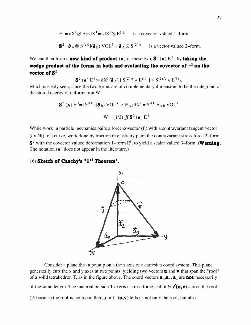
16) Sketch of Cauchy's "1st Theorem".
Consider a plane thru a point p on a the z axis of a cartesian coord system. This plane generically cuts the x and y axes at two points, yielding two vectors u and v that span the "roof" of a solid tetrahedron T, as in the figure above. The coord vectors ax,ay, az are not necessarily
of the same length. The material outside T exerts a stress force, call it ½ t (u,v) across the roof
(½ because the roof is not a parallelogram). (u,v) tells us not only the roof, but also
28
u, v, in that order is describing the normal pointing out of T. Likewise ½ t (v,u) describes a
force that the material in T exerts on material outside T. t (v,u) = - t (u,v) can be seen by
considering the equilibrium of a small thin disk with faces parallel to the plane spanned by u and v. This is the first part of Cauchy's 1st theorem. Stress forces act also on the coordinate faces. We now let the tetrahedron T shrink to the point p by moving the xy plane up to the point p, the dashed triangle showing an intermediate poition for the bottom face. At each stage the proportions of T are preserved. As the vertical edge ˜az˜ shrinks to 0, the stresses on the faces vanish as their areas, i.e., as ˜az˜2 while the body forces, e.g., gravity, if present, vanish as the volume ˜az˜3. We will neglect the body forces for vanishingly small T.
For our small T to be in equilibrium we must have, neglecting body forces
t (u,v) + t (az,ay) + t (ax ,az) + t (ay ,ax) — 0, and so
t (u,v)— - t (az ,ay) - t (ax ,az) - t (ay ,ax) i.e.,
t (u,v)— t (ay ,az) + t (az ,ax) + t (ax ,ay) (41)
Look at the first term t (ay ,az). The normal to the pair ay ,az is in the positive x
direction and so the area form for the y,z face is dy°dz. Let < t yz> be the area vector
dy°dz (ay , az) = dy°dz (u, v) and so t (ay ,az)= < t yz> dy°dz (u,v)
and similarly for the other faces in (41). We then have
t (u,v) — < t yz> dy°dz (u,v)+< t zx> dz°dx (u,v) + < t xy> dx°dy (u,v) (42)
29
Now as T shrinks to the point p the average < t yz> ‘ a vector t x(p)= t 1(p) at p, etc.
We can then approximate the stress in (42) , for a very small parallelogram at p spanned by u and v
t (u,v) — [t x(p) dy°dz + t y(p) dz°dx + t z(p) dx°dy ] (u,v)
which suggests Cauchy's theorem, that for any surface V2 with normal direction prescribed, the stress across V is given by a vector valued integral of the form
ˆV t x(x,y,z) dy°dz + t y(x,y,z) dz°dx + t z(x,y,z) dx°dy
with Cauchy vector valued stress 2-form
t 2 = t (2)j· i($ j) vol3 =
t x(x,y,z)·dy°dz + t y(x,y,z) ·dz°dx + t z (x,y,z)· dx°dy
The ith vector component of this form can be written t (2)i = t ij i($ j) vol3. Let us write this out in
classical engineering notation. If n is the unit normal to a surface element with area "form" dA, then i($ j) vol3, when evaluated on vectors tangent to V, is simply nj dA, where the components of the normal are nj = cos‚n,$ j ; this is simply the classical definition of the area form dA. Thus t (2)i = t ij nj dA, which is the classical expression for Cauchy stress.
17) Sketch of Cauchy's "2nd Theorem". Moments as generators of Rotations. For Cauchy's 2nd theorem, the symmetry of the stress tensor tij =tji, we shall consider only the simplest case of a deformed body, at rest and in equilibrium with its external tractions on its boundary, and with no external body forces (like gravity) considered. We employ Cartesian coords throughout. Then, since gij =∂ij, tensorial indices may be raised and lowered indiscriminately and we can use the summation convention for all repeated indices. Let B be any sub body in the interior of the body, with boundary $B. Then the (assumed vanishing) total stress force covector on B yields 0 = ˆ$B {dxc} · tcb i($b) vol3 = {dxc} ˆ$B t(2)c = {dxc} ˆB dt(2)c , where we use the braces { } just to remind us that the form to the left of · is a constant covector that plays no role in the integral. Since this holds for every interior B we must have dt(2)c = d tcb i($b) vol3 = 0 for each c (43)
30
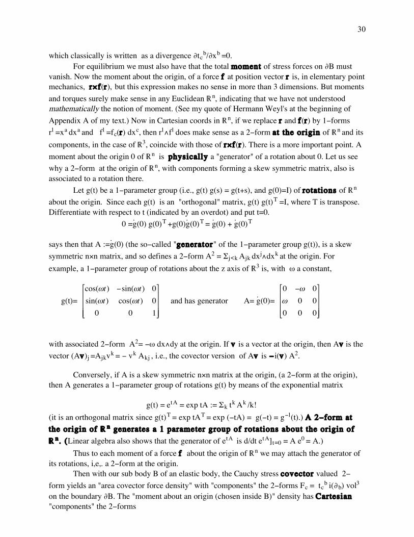
which classically is written as a divergence $tcb/$xb =0. For equilibrium we must also have that the total moment of stress forces on $B must vanish. Now the moment about the origin, of a force f at position vector r is, in elementary point mechanics, rªf(r), but this expression makes no sense in more than 3 dimensions. But moments and torques surely make sense in any Euclidean ®n, indicating that we have not understood mathematically the notion of moment. (See my quote of Hermann Weyl's at the beginning of Appendix A of my text.) Now in Cartesian coords in ®n, if we replace r and f(r) by 1-forms r1 =xa dxa and f1 =fc(r) dxc, then r1°f1 does make sense as a 2-form at the origin of ®n and its components, in the case of ®3, coincide with those of rªf(r). There is a more important point. A moment about the origin 0 of ®n is physically a "generator" of a rotation about 0. Let us see why a 2-form at the origin of ®n, with components forming a skew symmetric matrix, also is associated to a rotation there. Let g(t) be a 1-parameter group (i.e., g(t) g(s) = g(t+s), and g(0)=I) of rotations of ®n about the origin. Since each g(t) is an "orthogonal" matrix, g(t) g(t)T =I, where T is transpose. Differentiate with respect to t (indicated by an overdot) and put t=0. 0 =g‹(0) g(0)T +g(0)g‹(0)T = g‹(0) + g‹(0)T says then that A :=g‹(0) (the so-called "generator" of the 1-parameter group g(t)), is a skew symmetric nªn matrix, and so defines a 2-form A2 = ∑j<k Ajk dxj°dxk at the origin. For example, a 1-parameter group of rotations about the z axis of ®3 is, with ø a constant,
g(t)=
!
cos("t) #sin("t) 0
sin("t) cos("t) 0
0 0 1
$
%
& & &
'
(
) ) )
and has generator A= g‹(0)=
!
0 "# 0
# 0 0
0 0 0
$
%
& & &
'
(
) ) )
with associated 2-form A2= -ø dx°dy at the origin. If v is a vector at the origin, then Av is the vector (Av)j =Ajkvk = - vk Akj , i.e., the covector version of Av is -i(v) A2.
Conversely, if A is a skew symmetric nªn matrix at the origin, (a 2-form at the origin), then A generates a 1-parameter group of rotations g(t) by means of the exponential matrix
g(t) = etA = exp tA := ∑k tk Ak /k! (it is an orthogonal matrix since g(t)T = exp tAT = exp (-tA) = g(-t) = g-1(t).) A 2-form at the origin of ®n generates a 1 parameter group of rotations about the origin of ®n . (Linear algebra also shows that the generator of etA is d/dt etA]t=0 = A e0 = A.) Thus to each moment of a force f about the origin of ®n we may attach the generator of its rotations, i,e,. a 2-form at the origin. Then with our sub body B of an elastic body, the Cauchy stress covector valued 2-form yields an "area covector force density" with "components" the 2-forms Fc = tcb i($b) vol3 on the boundary $B. The "moment about an origin (chosen inside B)" density has Cartesian "components" the 2-forms
31
mac= [xa tcb -xc tab] i($b) vol3 = xa t(2)c -xc t(2)a Thus the total moment about the origin due to these stress forces on $B is the 2-form at the origin ∑a<c M ac dxa°dxc with components the numbers Mac = ˆ$B [xa t(2)c -xc t(2)a] = ˆB d [xa t(2)c -xc t(2)a] which, from (43), is Mac = ˆB dxa° t(2)c - dxc ° t(2)a In most common elastic materials, materials with no "micro structure", this must vanish if there are to be no internal rotations without internal torque sources. Since this holds for any portion B we must have dxa° t(2)c = dxc° t(2)a (44) Since these are 3-forms in ®3, dxa° t(2)c = dxa°tcbi($b) vol3= tca vol3. (44') For example, in ®3 with a=2 and c =1, dx2° t1b i($b) dx1°dx2°dx3 = dx2 ° t12 i($2) dx1°dx2°dx3 = - dx2 ° t12 i($2) dx2°dx1°dx3 = - dx2 ° t12 °dx1°dx3 = -t12 dx2° dx1°dx3 = t12 dx1° dx2°dx3 = t12 vol3
(44') then yields tca vol3 = tac vol3, and since coords are cartesian we have tca = tac. (45) Since the Cauchy stress t is a tensor, this symmetry holds in any coordinate system. This is Cauchy's 2nd Theorem. Warning. We have previously allowed and encouraged the use of different coordinates for the 2-form part and the value part of the stress vector valued 2-form, see e.g., p. 26 $ i· tij i($ j) vol3 = ea· Aai tij i($ j) vol3 = : ea· †aj i($ j) vol3. The left index "a" on † is always associated with the e basis and the right index "j" is always associated with the $ basis. (Think of e as cartesian and $ as cylindrical.) Does the fact that t is symmetric, tT = t, ensure that † = A t is also ? No! †T = tTAT = t AT = (A-1†) AT is generically ≠ †!
18) A Magic Formula for differentiating Line,and Surface, and . . . , Integrals. Let v be a time independent vector field in a coord patch U of ®n with any coords xi. Roughly speaking, i.e., omitting some technicalities, by integrating the differential equations dxi/dt = vi(x) we move along the integral curves of v for t seconds yielding a "flow" ƒt : U‘ ®n. Since v is time independent, the ƒt form a 1 parameter commutative group of mappings, ƒt ƒh = ƒt+h and ƒ0
is the identity map. Let Vr be an oriented r-dimensional "submanifold" of U. For examples, V1 is an oriented curve , V2 is an oriented 2 dimensional surface, ... . Vr is the kind of object over which one integrates an exterior r-form å=år,(a scalar valued, not vector valued form),
32
yielding the number ˆV år. As time changes, the flow moves V from V(0) =V to V(t)= ƒt (V). We consider only the simplest case where the r-form å is time-independent. How does the integral change in time? The answer can be shown to be
d/dt\t=0 ˆV(t) år = ˆVLvår (46)
where the r-form Lv år, the Lie derivative of the form å, is defined via the pullbacks
Furthermore, there is a remarkable expression for computing the Lie derivative given by the Henri Cartan (son of Elie Cartan) formula
Lv år = iv dår + d ivår (48)
Thus (46) and Stokes say
d/dt\t=0 ˆV(t) år = ˆVLvår = ˆV iv då + ˆ$V iv å (49)
Consider for example the case of a line integral in ®3, which we also write in classical form. V1 is then a curve C starting at point P and ending at point Q. Symbolically $C = Q -P.
Classically å = aÂdx. Then ivå is the 0-form, i.e., function vÂa, and ˆ$C vÂa is by definition simply vÂa(Q) - vÂa(P). This is the second "integral" in (49). Also, då1 is the 2-form version of the vector curl a, and so i v då , from (34), is the 1-form version of -vª curl a. We then have, in the classical version
The reader should work out the case of the 3-form vol3 in ®3.
References
T. Frankel, The Geometry of Physics, 2nd Ed. Cambridge University Press, 2004 F.D. Murnaghan, Finite deformation of an elastic solid , New York, Dover Publications [1967, c1951]