An Introduction to Multivariate Statistical Models

Statistical Methods for Psychologists, Part 4:

An Introduction to Multivariate Statistical Models

Douglas G. Bonett

University of California, Santa Cruz

2021

© All Rights Reserved

2

3

Contents

Chapter 1 Multivariate Statistical Models with Observed Variables

1.1 Introduction 1

1.2 Assessing Causality in Nonexperimental Designs 2

1.3 Path Diagram for a GLM 3

1.4 The lavaan R Package 4

1.5 Multivariate General Linear Models 7

1.6 Seemingly Unrelated Regression Models 9

1.7 Path Models 11

1.8 Path Models with Interaction Effects 15

1.9 Path Models with Categorical Moderators 18

1.10 Model Assessment in the GLM and MGLM 21

1.11 Model Assessment in SUR and Path Models 22

1.12 Assumptions 25

1.13 Missing Data 25

1.14 Assumption Diagnostics 26

Key Terms 27

Concept Questions 28

Data Analysis Problems 30

Chapter 2 Latent Factor Models

2.1 Measurement Error 33

2.2 Single-factor Model 35

2.3 General Latent Factor Model 36

2.4 Exploratory Factor Analysis 38

2.5 Parameter Estimation 40

2.6 Confidence Intervals for Factor Loadings and Unique Variances 41

2.7 Confidence Intervals for Correlations 43

2.8 Reliability Coefficients and Confidence Intervals 44

2.9 Second-order CFA Model 46

2.10 Bifactor CFA Model 48

2.11 Multiple-group CFA Model 50

2.12 CFA Model Assessment 52

2.13 Goodness-of-fit Tests 53

2.14 Model Comparison Tests 54

2.15 Fit Indices 55

2.16 Assumptions 57

2.17 Robust Methods 58

2.18 CFA for Ordinal Measurements 59

Key Terms 61



4

Chapter 3 Latent Variable Statistical Models

3.1 Advantages of Using Latent Variables 67

3.2 Latent Variable Regression Model 68

3.3 ANCOVA with Latent Covariates 70

3.4 MANOVA with Latent Response Variables 71

3.5 Latent Variable Path Model 73

3.6 Latent Growth Curve Models 74

3.7 Multiple-group Latent Variable Models 78

3.8 Model Assessment 80

3.9 Equivalent Models 83

3.10 Assumptions 83

3.11 Sample Size Recommendations 84

Key Terms 87



Appendix A. Tables 93

Appendix B. Glossary 97

Appendix C. Answers to Concept Questions 103

Appendix D. R Commands for Data Analysis Problems 113

1

Chapter 1

Multivariate Statistical Models with Observed Variables

1.1 Introduction

All of the statistical methods in this chapter expand upon the general linear model (GLM)

described in Chapter 2 of Part 2. Recall that the GLM can be used to assess the relations

between one quantitative response variable (y) and s predictor variables (𝑥1, 𝑥2, …, 𝑥𝑠).

The GLM is "general" in the sense that it can accommodate one or more fixed or random

predictor variables. The fixed predictor variables can be treatment factors or classification

factors. Furthermore, the GLM can include products of two predictor variables to

represent two-way interaction effects and squared predictor variables to accommodate

quadratic effects.

The GLM is a univariate statistical model because there is only one response variable. The

multivariate GLM (MGLM) is introduced in section 1.5 and can be used to assess the

relations between r > 1 response variables (𝑦1, 𝑦2, …, 𝑦𝑟) and s predictor variables. The

seemingly unrelated regression (SUR) model is introduced in section 1.6. The SUR model

allows each of the r response variables to have its own set of predictor variables. The path

model is introduced in section 1.7. Like the SUR model, the path model allows each of the

r response variables to have its own set of predictor variables and some response

variables (called mediator variables) can predict other response variables.

The MGLM, SUR, and path models can include product variables to assess interaction

effects and squared predictor variables to assess quadratic effects. Like the GLM, the

MGLM, SUR, and path models also can include fixed and random predictor variables.

Response variables and random predictor variables often contain considerable

measurement error. Measurement error can reduce the power of hypothesis tests,

increase the widths of confidence intervals, and introduce bias into slope and correlation

estimates. Statistical measurement models are introduced in Chapter 2. In Chapter 3,

measurement models are integrated into GLM, MGLM, SUR, and path models to reduce

the undesirable consequences of measurement error.

2

1.2 Assessing Causality in Nonexperimental Designs

Psychologists are ultimately interested in the discovery of causal relations. If x has a

causal effect on y, then changing the x score for a person will cause a change in that

person's predicted y score. However, if x and y are merely associated, then there is no

reason to believe that changing a person's x score will have any effect on that person's

predicted y score.

Recall from Chapter 2 of Part 1 that a predictor variable x will have a causal effect on a

response variable y if all of the following conditions are met: 1) x and y are related, 2) the

attribute measured by y occurred after the attribute measured by x, and 3) there are no

confounding variables. A confounding variable is related to both x and y and is assumed

to have a causal effect on x and y.

It is straightforward to determine if x and y are related (condition 1). For example, if x

and y are both quantitative variables, then a confidence interval for the population

Pearson correlation can be used to decide if the correlation is positive or negative and to

also assess the magnitude of the correlation. If x is a dummy coded variable and y is a

quantitative variable, then a confidence interval for a difference in population means or

a population standardized mean difference can be used to assess the direction and

strength of the relation.

Showing that the attribute measured by x occurred prior the attribute measure by y

(condition 2) can be difficult in a nonexperimental design. This requirement is

automatically satisfied in an experiment because participants are first exposed to a

treatment (x) and then following treatment their response (y) is measured. In a

nonexperimental design, if both x and y are measurements of transient states and x is

measured prior to y, then one could argue that the y attribute occurred after the x

attribute.

The requirement of no confounding variables (condition 3) will be satisfied in a properly

designed experiment. If participants are randomly assigned to the levels of x, then no

other variable can be related to x and hence there can be no confounding variables. In a

nonexperimental design, the relation between x and y will typically have numerous

confounding variables.

Suppose the researcher believes that 𝑥1 has a causal effect on y but it is not possible or

ethical to randomly assign participants to groups that receive different values of 𝑥1. To

assess a possible causal effect of 𝑥1 on y in a nonexperimental design, the researcher could

attempt to identify and measure as many confounding variables as possible and include

3

these confounding variables as additional predictor variables in a GLM. For example,

suppose three possible confounding variables are measured along with measurements of

𝑥1 and y in nonexperimental design. The GLM for this study would be

𝑦𝑖 = 𝛽0 + 𝛽1𝑥1𝑖 + 𝛽2𝑥2𝑖 + 𝛽3𝑥3𝑖 + 𝛽4𝑥4𝑖 + 𝑒𝑖 (Model 1.1)

where 𝑥2, 𝑥3, and 𝑥4 are the confounding variables. Recall from Chapter 2 of Part 2, that

𝛽1 does not describe the relation between y and 𝑥1 but instead describes the relation

between y and the component of 𝑥1 that is uncorrelated with the other predictor variables

in the model. This component was represented as 𝑒𝑥1because it is the prediction error in

a GLM that predicts 𝑥1 from the other predictor variables. We can replace 𝑥1 with 𝑒𝑥1 in

Model 1.1

𝑦𝑖 = 𝛽0 + 𝛽1𝑒𝑥1𝑖 + 𝛽2𝑥2𝑖 + 𝛽3𝑥3𝑖 + 𝛽4𝑥4𝑖 + 𝑒𝑖 (Model 1.2)

which does not change the value of 𝛽1. Prediction errors in a GLM are assumed to be

unrelated to the predictor variables and hence 𝑒𝑥1 is assumed to be unrelated with 𝑥2, 𝑥3,

and 𝑥4 in Model 1.2. If 𝑥2, 𝑥3, and 𝑥4 are unrelated to 𝑒𝑥1then they cannot be confounded

with 𝑒𝑥1. If the researcher can provide a convincing argument that 𝑥2, 𝑥3, and 𝑥4 are the

only confounding variables for 𝑥1, then the researcher also could argue that 𝛽1 describes

a causal effect of 𝑒𝑥1 on y.

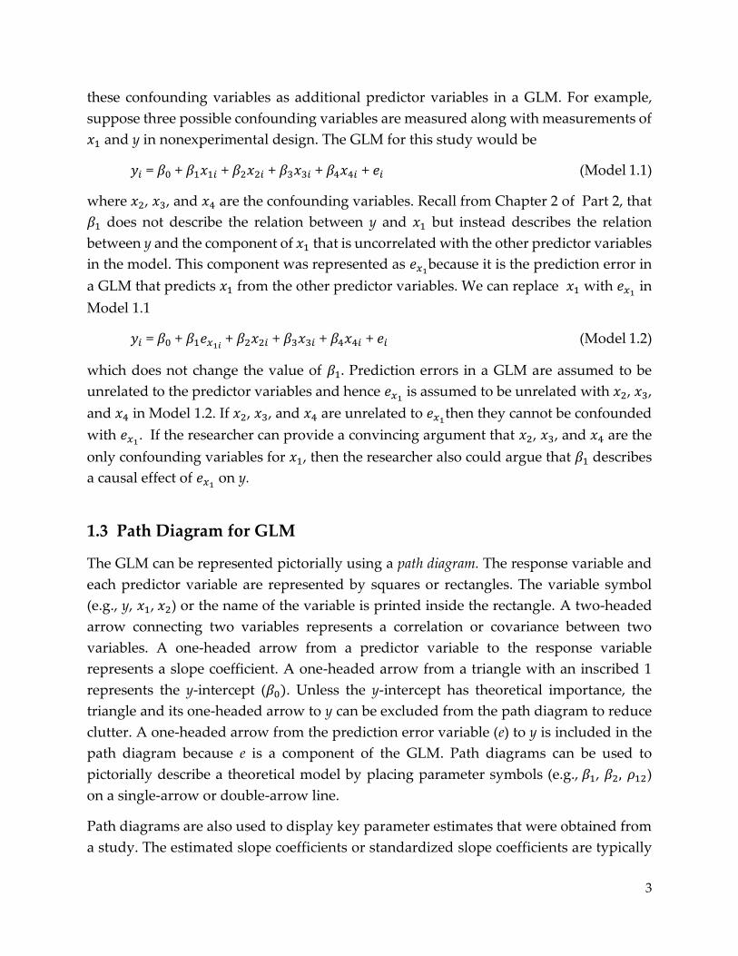
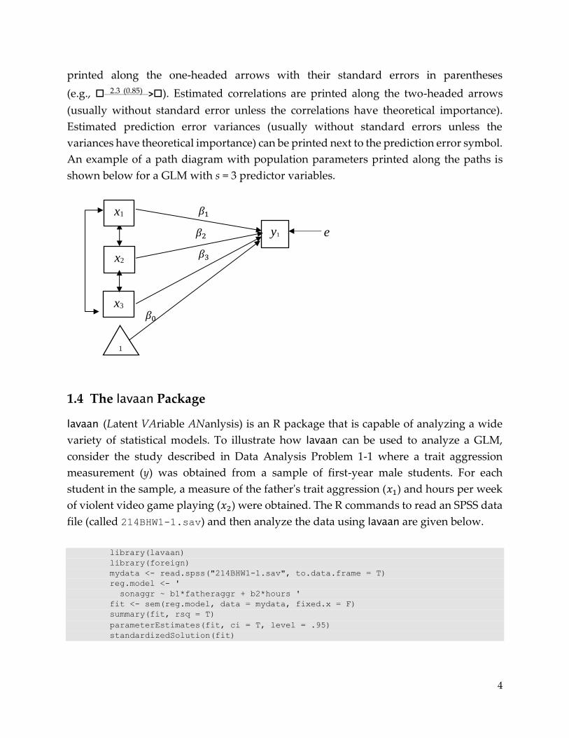
1.3 Path Diagram for GLM

The GLM can be represented pictorially using a path diagram. The response variable and

each predictor variable are represented by squares or rectangles. The variable symbol

(e.g., y, 𝑥1, 𝑥2) or the name of the variable is printed inside the rectangle. A two-headed

arrow connecting two variables represents a correlation or covariance between two

variables. A one-headed arrow from a predictor variable to the response variable

represents a slope coefficient. A one-headed arrow from a triangle with an inscribed 1

represents the y-intercept (𝛽0). Unless the y-intercept has theoretical importance, the

triangle and its one-headed arrow to y can be excluded from the path diagram to reduce

clutter. A one-headed arrow from the prediction error variable (e) to y is included in the

path diagram because e is a component of the GLM. Path diagrams can be used to

pictorially describe a theoretical model by placing parameter symbols (e.g., 𝛽1, 𝛽2, 𝜌12)

on a single-arrow or double-arrow line.

Path diagrams are also used to display key parameter estimates that were obtained from

a study. The estimated slope coefficients or standardized slope coefficients are typically

4

printed along the one-headed arrows with their standard errors in parentheses

(e.g., 2.3 (0.85) >). Estimated correlations are printed along the two-headed arrows

(usually without standard error unless the correlations have theoretical importance).

Estimated prediction error variances (usually without standard errors unless the

variances have theoretical importance) can be printed next to the prediction error symbol.

An example of a path diagram with population parameters printed along the paths is

shown below for a GLM with s = 3 predictor variables.

𝛽1

𝛽2 e

𝛽3

𝛽0

1.4 The lavaan Package

lavaan (Latent VAriable ANanlysis) is an R package that is capable of analyzing a wide

variety of statistical models. To illustrate how lavaan can be used to analyze a GLM,

consider the study described in Data Analysis Problem 1-1 where a trait aggression

measurement (y) was obtained from a sample of first-year male students. For each

student in the sample, a measure of the father's trait aggression (𝑥1) and hours per week

of violent video game playing (𝑥2) were obtained. The R commands to read an SPSS data

file (called 214BHW1-1.sav) and then analyze the data using lavaan are given below.

library(lavaan)

library(foreign)

mydata <- read.spss("214BHW1-1.sav", to.data.frame = T)

reg.model <- '

sonaggr ~ b1*fatheraggr + b2*hours '

fit <- sem(reg.model, data = mydata, fixed.x = F)

summary(fit, rsq = T)

parameterEstimates(fit, ci = T, level = .95)

standardizedSolution(fit)

x3

x2

y1

1y1

1

x1

5

The library(lavaan) command instructs R to load the lavaan package. The

library(foreign) command instructs R to load the foreign package which allows

the user to read data files that were created from other statistical packages such as SPSS.

The mydata <- read.spss("214BHW1-1.sav", to.data.frame = T) command

instructs R to read an SPSS data file named 214BHW1-1.sav in the default working

directory and assigns it a user-given object name of mydata.

The code reg.model <- 'sonaggr ~ b1*fatheraggr + b2*hours' defines the model

and assigns it a user-given object name of reg.model. The model definition is specified

within single quotes. The variable name (e.g. sonaggr) for the response variable is on the

left of the ~ symbol (which stands for “regress onto”), and the other variables that are on

the right of the ~ symbol and separated with + signs (e.g., fatheraggr and hours) specify

the predictor variables in the model. The b1 and b2 names are optional user-given

parameter labels that are followed by the * command and are needed to perform more

complicated analyses that will be described later.

The code fit <- sem(reg.model, data = mydata, fixed.x = F) calls the sem

function within lavaan to analyze the model specified in reg.model using the data

assigned to mydata. T and F are abbreviations for True and False. The fixed.x = F

option species a random-x model (i.e., not a fixed-x model). The results (i.e., parameter

estimates, standard errors, test statistics) are assigned to the user-given object name fit.

The summary(fit, rsq = T)command instructs lavaan to print the statistical results

that have been assigned to fit and to also include an estimate of the squared multiple

correlation. The parameterEstimates(fit, ci = T, level = .95)command instructs

lavaan to compute 95% confidence intervals for the model parameters. The

standardizedSolution(fit) command instructs lavaan to print estimates,

approximate standard errors, and confidence intervals for standardized slope coefficients

and standardized covariances (a standardized covariance is a correlation coefficient).

Although a GLM can be easily analyzed in SPSS and other programs, some specialized

GLM analyses that are easy to perform in lavaan are not possible in the basic GLM

programs. For example, with lavaan it is easy to obtain condition slopes and their

confidence intervals, an estimated maximum or minimum in a quadratic model, and

confidence intervals for standardized slopes. These capabilities are illustrated in the

following examples.

Suppose we have the following GLM with predictor variables 𝑥1 and 𝑥2 and an

interaction between 𝑥1 and 𝑥2

6

𝑦𝑖 = 𝛽0 + 𝛽1𝑥1𝑖 + 𝛽2𝑥2𝑖 + 𝛽3𝑥3𝑖 + 𝑒𝑖 (Model 1.3)

where 𝑥3𝑖 = 𝑥1𝑖𝑥2𝑖. The conditional slope for 𝑥1 at 𝑥2∗ (where 𝑥2

∗ is some value of

𝑥2 specified by the researcher) is defined as 𝛽1 + 𝛽3𝑥2∗.

Suppose 𝑥1 = sex (dummy coded), 𝑥2 = GPA, and 𝑥3 = sex*GPA (and named “interaction”

in the data file). The researcher wants to estimate the conditional slopes for sex at GPA =

2.5 and at GPA = 3.7. The := command can be used to define a new parameter that is a

linear or nonlinear function of the model parameters. The model definition and the

defined conditional slopes is shown below where slopeAt2.5 and slopeAt3.7 are user-

given names to the two conditional slopes. Note that the optional parameter labels b1

and b2 were needed to define the conditional slopes.

reg.model <- '

score ~ b1*sex + b2*GPA + b3*interaction

slopeAt2.5 := b1 + b3*2.5

slopeAt3.7 := b1 + b3*3.7 '

fit <- sem(reg.model, data = mydata, fixed.x = F) parameterEstimates(fit, ci = T, level = .95)

The output will include estimates of the two conditional slopes and their standard errors.

The parameterEstimates(fit, ci = T, level = .95)command instructs lavaan to

compute 95% confidence intervals for the model parameters and conditional slopes.

Adding a standardizedSolution(fit) command to the above code would instructs

lavaan to compute standardized slopes and conditional slopes along with their standard

errors.

In a quadratic model 𝑦𝑖 = 𝛽0 + 𝛽1𝑥1𝑖 + 𝛽2𝑥1𝑖2 + 𝑒𝑖, the relation between x and y is assumed

to be curved with one bend. The slope of a line tangent to the curve at 𝑥1∗ is equal to

𝛽1 + 2𝛽2𝑥1∗ . The value of 𝑥1 where the curve is at its minimum or maximum is -𝛽1/2𝛽2

and corresponds to the point where the slope of the tangent line is equal to 0.

Consider an experiment where participants are randomly assigned to receive 0 mg

(placebo), 100 mg, 200 mg, or 400 mg of caffeine and y is a score on a cognitive ability test.

To estimate the dosage (𝑥1) that maximizes performance on the cognitive test and to also

estimate the slope of the line tangent to the curve at 𝑥1∗ = 300 mg, the following lavaan

model specification code can be used (where the data file contains the variables

testscore, dose, and dosesqr) which computes estimates of optimumdose and

slopeAt300 and their standard errors. A parameterEstimates(fit, ci = T, level =

.95)command can be added to the following code to obtain 95% confidence intervals for

the optimal dose and the slope at 300 mg.

7

quad.model <- '

testscore ~ b1*dose + b2*dosesqr

optimumdose := -b1/(2*b2)

slopeAt300 := b1 + 2*b2*300 '

fit <- sem(quad.model, data = mydata, fixed.x = F)

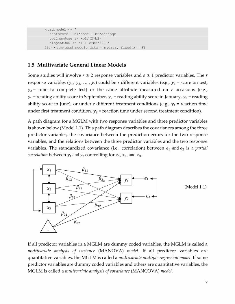
1.5 Multivariate General Linear Models

Some studies will involve r ≥ 2 response variables and s ≥ 1 predictor variables. The r

response variables (𝑦1, 𝑦2, … , 𝑦𝑟) could be r different variables (e.g., 𝑦1 = score on test,

𝑦2 = time to complete test) or the same attribute measured on r occasions (e.g.,

𝑦1 = reading ability score in September, 𝑦2 = reading ability score in January, 𝑦3 = reading

ability score in June), or under r different treatment conditions (e.g., 𝑦1 = reaction time

under first treatment condition, 𝑦2 = reaction time under second treatment condition).

A path diagram for a MGLM with two response variables and three predictor variables

is shown below (Model 1.1). This path diagram describes the covariances among the three

predictor variables, the covariance between the prediction errors for the two response

variables, and the relations between the three predictor variables and the two response

variables. The standardized covariance (i.e., correlation) between 𝑒1 and 𝑒2 is a partial

correlation between 𝑦1 and 𝑦2 controlling for 𝑥1, 𝑥2, and 𝑥3.

𝛽11

𝛽12 𝛽21 e1

𝛽22 (Model 1.1)

𝛽31 e2

𝛽32

𝛽01

𝛽02

If all predictor variables in a MGLM are dummy coded variables, the MGLM is called a

multivariate analysis of variance (MANOVA) model. If all predictor variables are

quantitative variables, the MGLM is called a multivariate multiple regression model. If some

predictor variables are dummy coded variables and others are quantitative variables, the

MGLM is called a multivariate analysis of covariance (MANCOVA) model.

x1

y1

1y1

1

x3

x2

y2

8

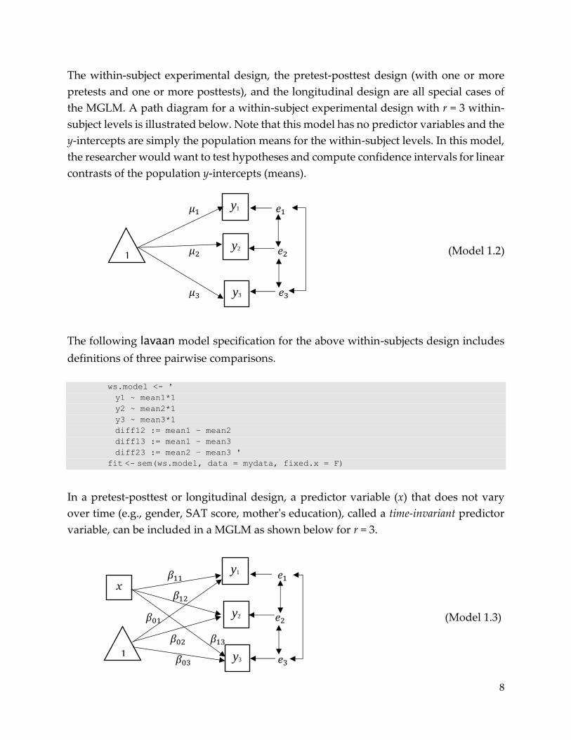
The within-subject experimental design, the pretest-posttest design (with one or more

pretests and one or more posttests), and the longitudinal design are all special cases of

the MGLM. A path diagram for a within-subject experimental design with r = 3 within-

subject levels is illustrated below. Note that this model has no predictor variables and the

y-intercepts are simply the population means for the within-subject levels. In this model,

the researcher would want to test hypotheses and compute confidence intervals for linear

contrasts of the population y-intercepts (means).

𝜇1 𝑒1

𝜇2 𝑒2 (Model 1.2)

𝜇3 𝑒3

The following lavaan model specification for the above within-subjects design includes

definitions of three pairwise comparisons.

ws.model <- '

y1 ~ mean1*1

y2 ~ mean2*1

y3 ~ mean3*1

diff12 := mean1 – mean2

diff13 := mean1 – mean3

diff23 := mean2 – mean3 '

fit <- sem(ws.model, data = mydata, fixed.x = F)

In a pretest-posttest or longitudinal design, a predictor variable (x) that does not vary

over time (e.g., gender, SAT score, mother's education), called a time-invariant predictor

variable, can be included in a MGLM as shown below for r = 3.

𝛽11 𝑒1

𝛽12

𝛽01 𝑒2 (Model 1.3)

𝛽02 𝛽13

𝛽03 𝑒3

y1

y3

x

1

y1

y2

y3

1 y2

9

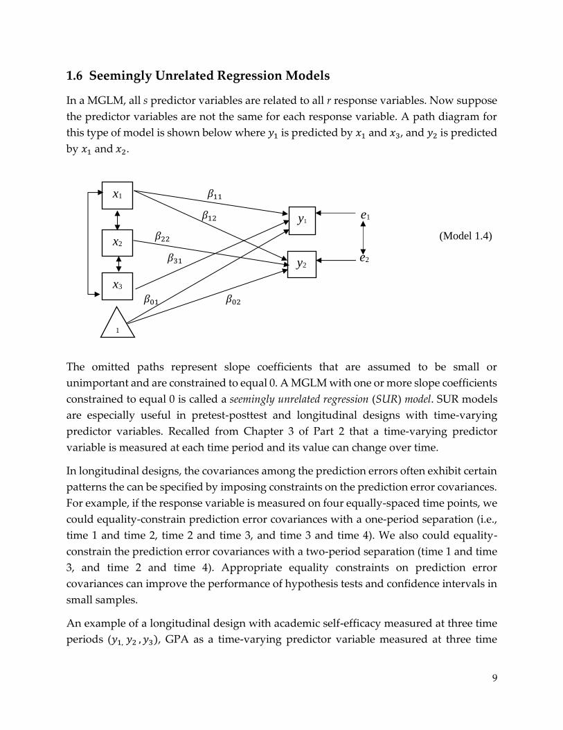
1.6 Seemingly Unrelated Regression Models

In a MGLM, all s predictor variables are related to all r response variables. Now suppose

the predictor variables are not the same for each response variable. A path diagram for

this type of model is shown below where 𝑦1 is predicted by 𝑥1 and 𝑥3, and 𝑦2 is predicted

by 𝑥1 and 𝑥2.

𝛽11

𝛽12 e1

𝛽22 (Model 1.4)

𝛽31 e2

𝛽01 𝛽02

The omitted paths represent slope coefficients that are assumed to be small or

unimportant and are constrained to equal 0. A MGLM with one or more slope coefficients

constrained to equal 0 is called a seemingly unrelated regression (SUR) model. SUR models

are especially useful in pretest-posttest and longitudinal designs with time-varying

predictor variables. Recalled from Chapter 3 of Part 2 that a time-varying predictor

variable is measured at each time period and its value can change over time.

In longitudinal designs, the covariances among the prediction errors often exhibit certain

patterns the can be specified by imposing constraints on the prediction error covariances.

For example, if the response variable is measured on four equally-spaced time points, we

could equality-constrain prediction error covariances with a one-period separation (i.e.,

time 1 and time 2, time 2 and time 3, and time 3 and time 4). We also could equality-

constrain the prediction error covariances with a two-period separation (time 1 and time

3, and time 2 and time 4). Appropriate equality constraints on prediction error

covariances can improve the performance of hypothesis tests and confidence intervals in

small samples.

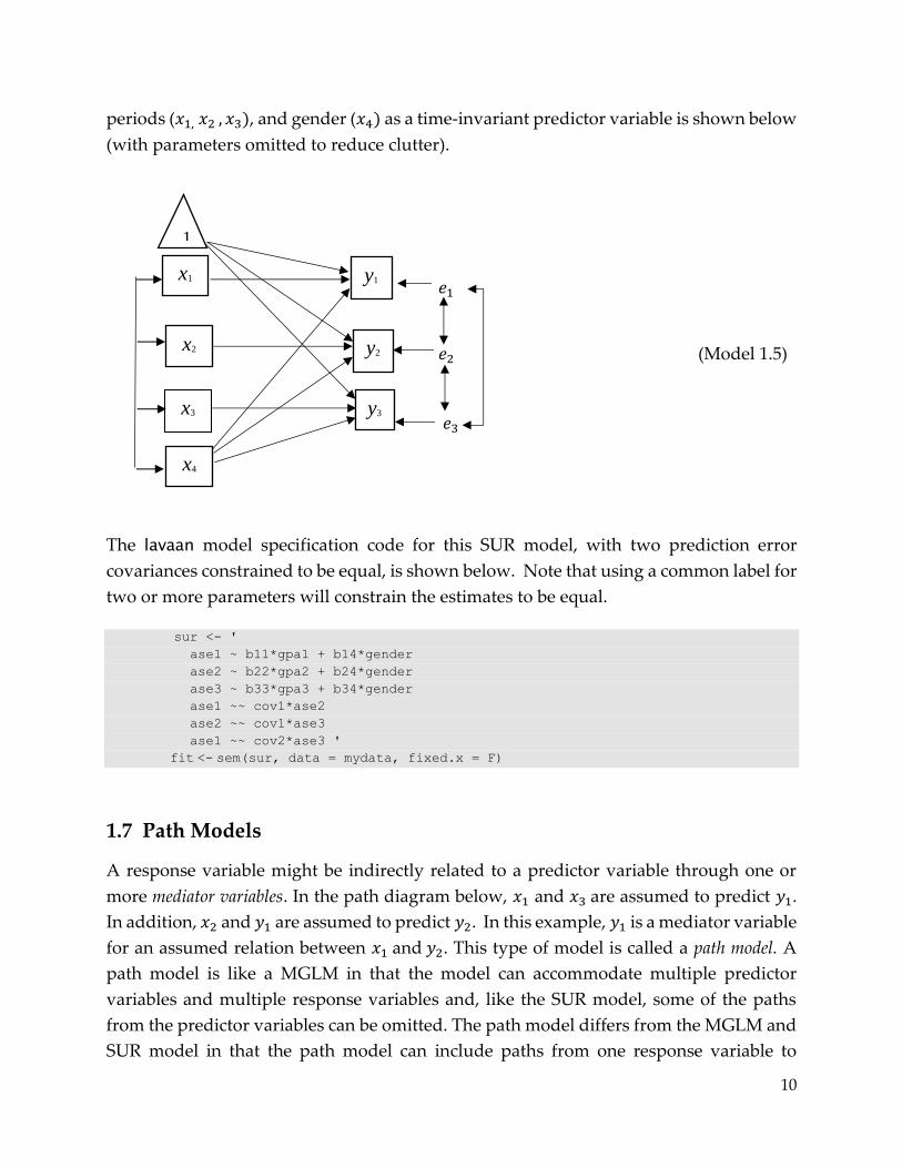
An example of a longitudinal design with academic self-efficacy measured at three time

periods (𝑦1, 𝑦2 , 𝑦3), GPA as a time-varying predictor variable measured at three time

x1

x3

1

x2

y1

1y

1

y2

10

periods (𝑥1, 𝑥2 , 𝑥3), and gender (𝑥4) as a time-invariant predictor variable is shown below

(with parameters omitted to reduce clutter).

𝑒1

𝑒2 (Model 1.5)

𝑒3

The lavaan model specification code for this SUR model, with two prediction error

covariances constrained to be equal, is shown below. Note that using a common label for

two or more parameters will constrain the estimates to be equal.

sur <- '

ase1 ~ b11*gpa1 + b14*gender



ase1 ~~ cov1*ase2

ase2 ~~ cov1*ase3

ase1 ~~ cov2*ase3 '

fit <- sem(sur, data = mydata, fixed.x = F)

1.7 Path Models

A response variable might be indirectly related to a predictor variable through one or

more mediator variables. In the path diagram below, 𝑥1 and 𝑥3 are assumed to predict 𝑦1.

In addition, 𝑥2 and 𝑦1 are assumed to predict 𝑦2. In this example, 𝑦1 is a mediator variable

for an assumed relation between 𝑥1 and 𝑦2. This type of model is called a path model. A

path model is like a MGLM in that the model can accommodate multiple predictor

variables and multiple response variables and, like the SUR model, some of the paths

from the predictor variables can be omitted. The path model differs from the MGLM and

SUR model in that the path model can include paths from one response variable to

y1 x1

y3 x3

1

y2 x2

x4

11

another response variable. The path coefficient describing the effect of 𝑦𝑗 on 𝑦𝑘 is denoted

as 𝛾𝑗𝑘 and represents the change in 𝑦𝑘 associated with a 1-unit increase in 𝑦𝑗, controlling

for all other predictors of 𝑦𝑘.

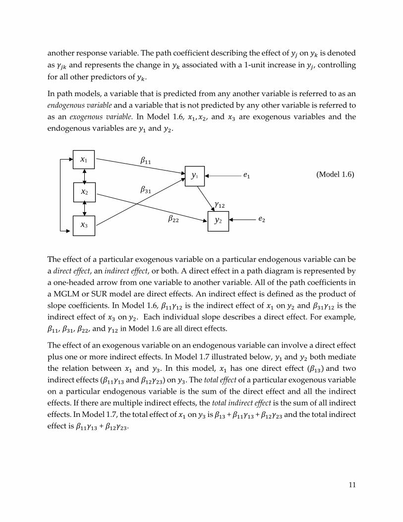
In path models, a variable that is predicted from any another variable is referred to as an

endogenous variable and a variable that is not predicted by any other variable is referred to

as an exogenous variable. In Model 1.6, 𝑥1, 𝑥2, and 𝑥3 are exogenous variables and the

endogenous variables are 𝑦1 and 𝑦2.

𝛽11

𝑒1 (Model 1.6)

𝛽31

𝛾12

𝛽22 𝑒2

The effect of a particular exogenous variable on a particular endogenous variable can be

a direct effect, an indirect effect, or both. A direct effect in a path diagram is represented by

a one-headed arrow from one variable to another variable. All of the path coefficients in

a MGLM or SUR model are direct effects. An indirect effect is defined as the product of

slope coefficients. In Model 1.6, 𝛽11𝛾12 is the indirect effect of 𝑥1 on 𝑦2 and 𝛽31𝛾12 is the

indirect effect of 𝑥3 on 𝑦2. Each individual slope describes a direct effect. For example,

𝛽11, 𝛽31, 𝛽22, and 𝛾12 in Model 1.6 are all direct effects.

The effect of an exogenous variable on an endogenous variable can involve a direct effect

plus one or more indirect effects. In Model 1.7 illustrated below, 𝑦1 and 𝑦2 both mediate

the relation between 𝑥1 and 𝑦3. In this model, 𝑥1 has one direct effect (𝛽13) and two

indirect effects (𝛽11𝛾13 and 𝛽12𝛾23) on 𝑦3. The total effect of a particular exogenous variable

on a particular endogenous variable is the sum of the direct effect and all the indirect

effects. If there are multiple indirect effects, the total indirect effect is the sum of all indirect

effects. In Model 1.7, the total effect of 𝑥1 on 𝑦3 is 𝛽13 + 𝛽11𝛾13 + 𝛽12𝛾23 and the total indirect

effect is 𝛽11𝛾13 + 𝛽12𝛾23.

x1

x3

x2

y1

1y1

y2

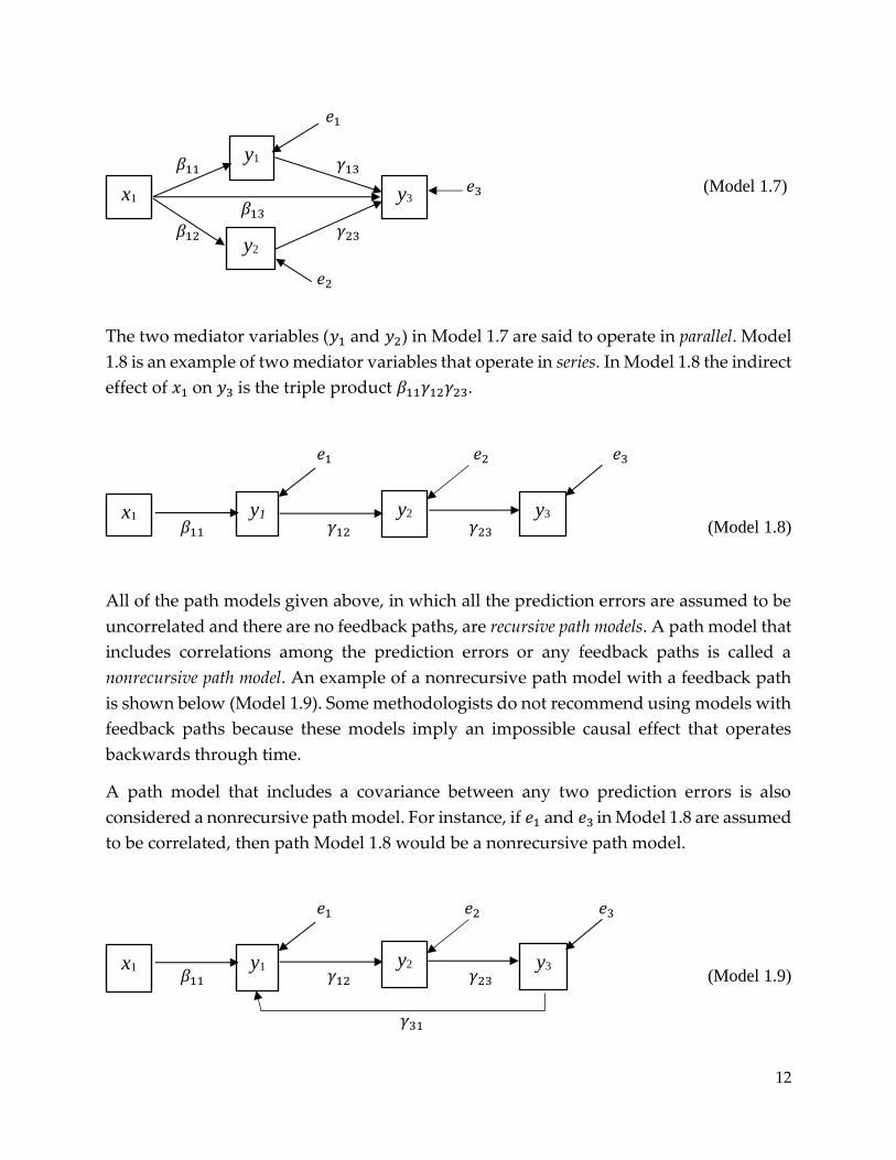
12

𝑒1

𝛽11 𝛾13 𝑒3 (Model 1.7)

𝛽13 𝛽12 𝛾23

𝑒2

The two mediator variables (𝑦1 and 𝑦2) in Model 1.7 are said to operate in parallel. Model

1.8 is an example of two mediator variables that operate in series. In Model 1.8 the indirect

effect of 𝑥1 on 𝑦3 is the triple product 𝛽11𝛾12𝛾23.

𝑒1 𝑒2 𝑒3

𝛽11 𝛾12 𝛾23 (Model 1.8)

All of the path models given above, in which all the prediction errors are assumed to be

uncorrelated and there are no feedback paths, are recursive path models. A path model that

includes correlations among the prediction errors or any feedback paths is called a

nonrecursive path model. An example of a nonrecursive path model with a feedback path

is shown below (Model 1.9). Some methodologists do not recommend using models with

feedback paths because these models imply an impossible causal effect that operates

backwards through time.

A path model that includes a covariance between any two prediction errors is also

considered a nonrecursive path model. For instance, if 𝑒1 and 𝑒3 in Model 1.8 are assumed

to be correlated, then path Model 1.8 would be a nonrecursive path model.

𝑒1 𝑒2 𝑒3

𝛽11 𝛾12 𝛾23 (Model 1.9)

𝛾31

y1

y2

x1 y1 y3 y2

x1 y3

x1 y1 y3 y2

13

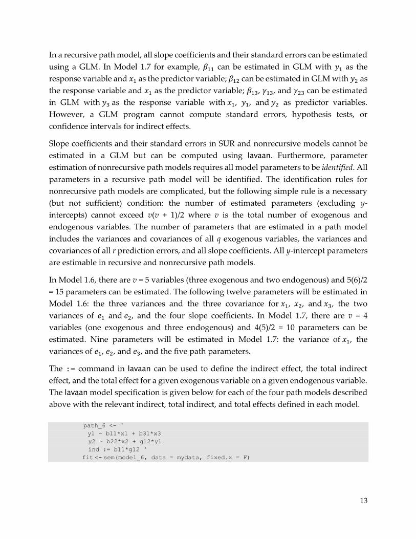
In a recursive path model, all slope coefficients and their standard errors can be estimated

using a GLM. In Model 1.7 for example, 𝛽11 can be estimated in GLM with 𝑦1 as the

response variable and 𝑥1 as the predictor variable; 𝛽12 can be estimated in GLM with 𝑦2 as

the response variable and 𝑥1 as the predictor variable; 𝛽13, 𝛾13, and 𝛾23 can be estimated

in GLM with 𝑦3 as the response variable with 𝑥1, 𝑦1, and 𝑦2 as predictor variables.

However, a GLM program cannot compute standard errors, hypothesis tests, or

confidence intervals for indirect effects.

Slope coefficients and their standard errors in SUR and nonrecursive models cannot be

estimated in a GLM but can be computed using lavaan. Furthermore, parameter

estimation of nonrecursive path models requires all model parameters to be identified. All

parameters in a recursive path model will be identified. The identification rules for

nonrecursive path models are complicated, but the following simple rule is a necessary

(but not sufficient) condition: the number of estimated parameters (excluding y-

intercepts) cannot exceed v(v + 1)/2 where v is the total number of exogenous and

endogenous variables. The number of parameters that are estimated in a path model

includes the variances and covariances of all q exogenous variables, the variances and

covariances of all r prediction errors, and all slope coefficients. All y-intercept parameters

are estimable in recursive and nonrecursive path models.

In Model 1.6, there are v = 5 variables (three exogenous and two endogenous) and 5(6)/2

= 15 parameters can be estimated. The following twelve parameters will be estimated in

Model 1.6: the three variances and the three covariance for 𝑥1, 𝑥2, and 𝑥3, the two

variances of 𝑒1 and 𝑒2, and the four slope coefficients. In Model 1.7, there are v = 4

variables (one exogenous and three endogenous) and 4(5)/2 = 10 parameters can be

estimated. Nine parameters will be estimated in Model 1.7: the variance of 𝑥1, the

variances of 𝑒1, 𝑒2, and 𝑒3, and the five path parameters.

The := command in lavaan can be used to define the indirect effect, the total indirect

effect, and the total effect for a given exogenous variable on a given endogenous variable.

The lavaan model specification is given below for each of the four path models described

above with the relevant indirect, total indirect, and total effects defined in each model.

path_6 <- '

y1 ~ b11*x1 + b31*x3

y2 ~ b22*x2 + g12*y1

ind := b11*g12 '

fit <- sem(model_6, data = mydata, fixed.x = F)

14

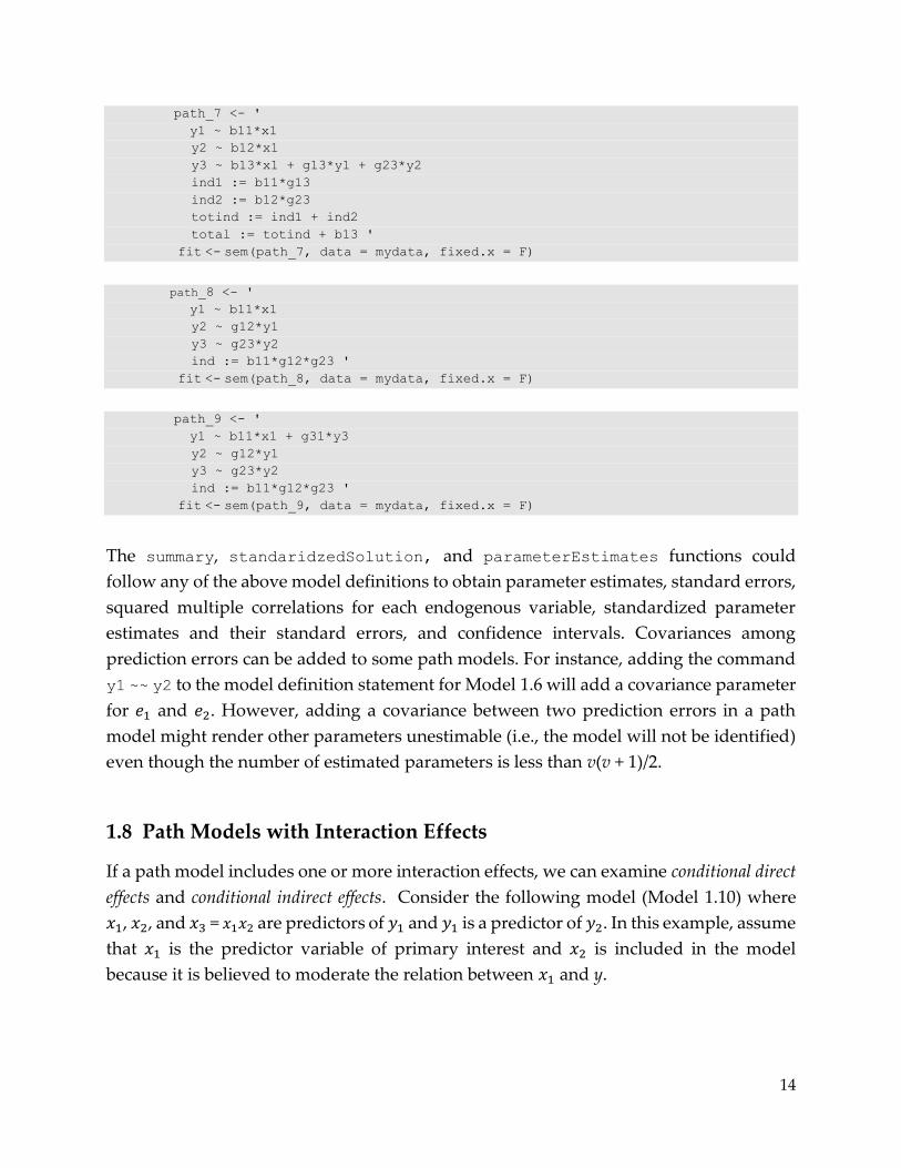
path_7 <- '

y1 ~ b11*x1

y2 ~ b12*x1

y3 ~ b13*x1 + g13*y1 + g23*y2

ind1 := b11*g13

ind2 := b12*g23

totind := ind1 + ind2

total := totind + b13 '

fit <- sem(path_7, data = mydata, fixed.x = F)

path_8 <- '

y1 ~ b11*x1

y2 ~ g12*y1

y3 ~ g23*y2

ind := b11*g12*g23 '


path_9 <- '

y1 ~ b11*x1 + g31*y3

y2 ~ g12*y1

y3 ~ g23*y2

ind := b11*g12*g23 '


The summary, standaridzedSolution, and parameterEstimates functions could

follow any of the above model definitions to obtain parameter estimates, standard errors,

squared multiple correlations for each endogenous variable, standardized parameter

estimates and their standard errors, and confidence intervals. Covariances among

prediction errors can be added to some path models. For instance, adding the command

y1 ~~ y2 to the model definition statement for Model 1.6 will add a covariance parameter

for 𝑒1 and 𝑒2. However, adding a covariance between two prediction errors in a path

model might render other parameters unestimable (i.e., the model will not be identified)

even though the number of estimated parameters is less than v(v + 1)/2.

1.8 Path Models with Interaction Effects

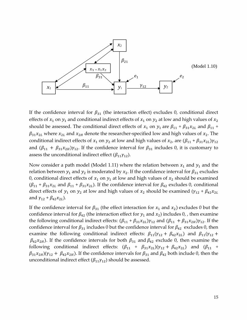
If a path model includes one or more interaction effects, we can examine conditional direct

effects and conditional indirect effects. Consider the following model (Model 1.10) where

𝑥1, 𝑥2, and 𝑥3 = 𝑥1𝑥2 are predictors of 𝑦1 and 𝑦1 is a predictor of 𝑦2. In this example, assume

that 𝑥1 is the predictor variable of primary interest and 𝑥2 is included in the model

because it is believed to moderate the relation between 𝑥1 and y.

15

𝛽21 (Model 1.10)

𝛽31 𝑒1 𝑒2

𝛽11 𝛾12

If the confidence interval for 𝛽31 (the interaction effect) excludes 0, conditional direct

effects of 𝑥1 on 𝑦1 and conditional indirect effects of 𝑥1 on 𝑦2 at low and high values of 𝑥2

should be assessed. The conditional direct effects of 𝑥1 on 𝑦1 are 𝛽11 + 𝛽31𝑥2𝐿 and 𝛽11 +

𝛽31𝑥2𝐿 where 𝑥2𝐿 and 𝑥2𝐻 denote the researcher-specified low and high values of 𝑥2. The

conditional indirect effects of 𝑥1 on 𝑦2 at low and high values of 𝑥2, are (𝛽11 + 𝛽31𝑥2𝐿)𝛾12

and (𝛽11 + 𝛽31𝑥2𝐻)𝛾12. If the confidence interval for 𝛽31 includes 0, it is customary to

assess the unconditional indirect effect (𝛽11𝛾12).

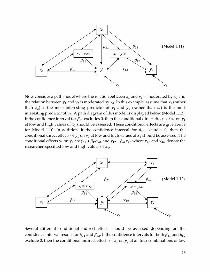
Now consider a path model (Model 1.11) where the relation between 𝑥1 and 𝑦1 and the

relation between 𝑦1 and 𝑦2 is moderated by 𝑥2. If the confidence interval for 𝛽31 excludes

0, conditional direct effects of 𝑥1 on 𝑦1 at low and high values of 𝑥2 should be examined

(𝛽11 + 𝛽31𝑥2𝐿 and 𝛽11 + 𝛽31𝑥2𝐿). If the confidence interval for 𝛽42 excludes 0, conditional

direct effects of 𝑦1 on 𝑦2 at low and high values of 𝑥2 should be examined (𝛾12 + 𝛽42𝑥2𝐿

and 𝛾12 + 𝛽42𝑥2𝐿).

If the confidence interval for 𝛽31 (the effect interaction for 𝑥1 and 𝑥2) excludes 0 but the

confidence interval for 𝛽42 (the interaction effect for 𝑦1 and 𝑥2) includes 0, , then examine

the following conditional indirect effects: (𝛽11 + 𝛽31𝑥2𝐿)𝛾12 and (𝛽11 + 𝛽31𝑥2𝐻)𝛾12. If the

confidence interval for 𝛽31 includes 0 but the confidence interval for 𝛽42 excludes 0, then

examine the following conditional indirect effects: 𝛽11(𝛾12 + 𝛽42𝑥2𝐿) and 𝛽11(𝛾12 +

𝛽42𝑥2𝐻). If the confidence intervals for both 𝛽31 and 𝛽42 exclude 0, then examine the

following conditional indirect effects: (𝛽11 + 𝛽31𝑥2𝐿)(𝛾12 + 𝛽42𝑥2𝐿) and (𝛽11 +

𝛽31𝑥2𝐻)(𝛾12 + 𝛽42𝑥2𝐻). If the confidence intervals for 𝛽31 and 𝛽42 both include 0, then the

unconditional indirect effect (𝛽11𝛾12) should be assessed.

𝑥3 = 𝑥1𝑥2

x1

==𝛾12𝛾12

x2

x1 y2 y1

1y1

16

𝛽21 𝛽22 (Model 1.11)

𝛽31 𝛽42

𝛽11 𝛾12

𝑒1 𝑒2

Now consider a path model where the relation between 𝑥1 and 𝑦1 is moderated by 𝑥2 and

the relation between 𝑦1 and 𝑦2 is moderated by 𝑥4. In this example, assume that 𝑥1 (rather

than 𝑥2) is the most interesting predictor of 𝑦1 and 𝑦1 (rather than 𝑥4) is the most

interesting predictor of 𝑦2. A path diagram of this model is displayed below (Model 1.12).

If the confidence interval for 𝛽31 excludes 0, then the conditional direct effects of 𝑥1 on 𝑦1

at low and high values of 𝑥2 should be assessed. These conditional effects are give above

for Model 1.10. In addition, if the confidence interval for 𝛽42 excludes 0, then the

conditional direct effects of 𝑦1 on 𝑦2 at low and high values of 𝑥4 should be assessed. The

conditional effects 𝑦1 on 𝑦2 are 𝛾12 + 𝛽42𝑥4𝐿 and 𝛾12 + 𝛽42𝑥4𝐿 where 𝑥4𝐿 and 𝑥4𝐻 denote the

researcher-specified low and high values of 𝑥4.

𝛽21 𝛽42 (Model 1.12)

𝛽31 𝛽52

𝛽11 𝛾12

𝑒1 𝑒2

Several different conditional indirect effects should be assessed depending on the

confidence interval results for 𝛽31 and 𝛽52. If the confidence intervals for both 𝛽31 and 𝛽52

exclude 0, then the conditional indirect effects of 𝑥1 on 𝑦2 at all four combinations of low

x3 = x1x2

x1

==

𝛾12𝛾12

x1

x3 = x1x2

x1

==

𝛾12𝛾12

x4

4

x2

x5 = y1x4

x4 = y1x2

y2 y1

1y1

x1 y2

x2

y1

1y1

17

and high values of 𝑥2 and 𝑥4 should be assessed. These four conditional indirect effects

are: (𝛽11 + 𝛽31𝑥2𝐿)(𝛾12 + 𝛽52𝑥4𝐿), (𝛽11 + 𝛽31𝑥2𝐻)(𝛾12 + 𝛽52𝑥4𝐿), (𝛽11 + 𝛽31𝑥2𝐿)(𝛾12 + 𝛽52𝑥4𝐻),

and (𝛽11 + 𝛽31𝑥2𝐻)(𝛾12 + 𝛽52𝑥4𝐻).

If the confidence interval for 𝛽31 excludes 0 but the confidence interval for 𝛽52 includes 0,

then the conditional indirect effects of 𝑥1 on 𝑦2 at low and high values of 𝑥2 should be

assessed. These conditional indirect effects are (𝛽11 + 𝛽31𝑥2𝐿)𝛾12 and (𝛽11 + 𝛽31𝑥2𝐻)𝛾12.

If the confidence interval for 𝛽52 excludes 0 but the confidence interval for 𝛽31 includes 0,

then the conditional indirect effects of 𝑥1 on 𝑦2 at low and high values of 𝑥4 should be

assessed. These conditional indirect effects are 𝛽11(𝛾12 + 𝛽52𝑥4𝐿) and 𝛽11(𝛾12 + 𝛽52𝑥4𝐻).

If the confidence intervals for 𝛽31 and 𝛽52 both include 0, then the unconditional indirect

effect (𝛽11𝛾12) should be assessed.

Slopes coefficients in path coefficients are often interpreted as causal effects. It is

important to remember that slope coefficients in a path model are also susceptible to

confounding variable bias, and all of the concerns about interpreting GLM slope

coefficients in nonexperimental designs also apply to path models.

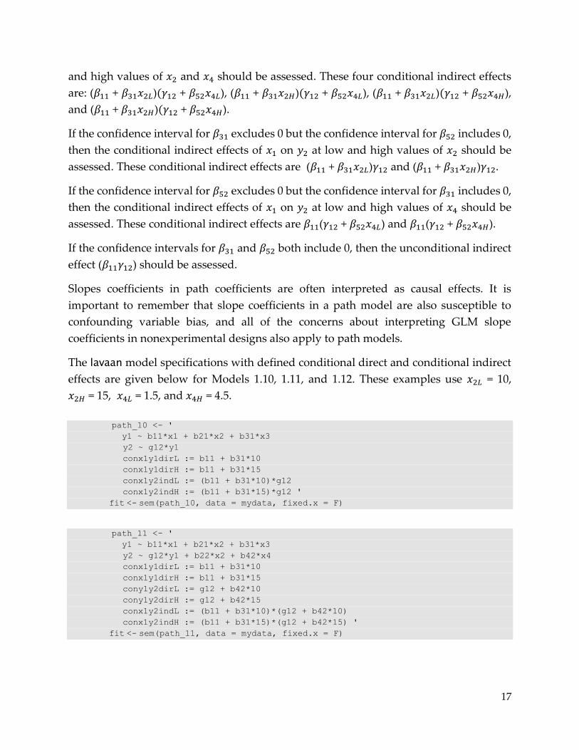
The lavaan model specifications with defined conditional direct and conditional indirect

effects are given below for Models 1.10, 1.11, and 1.12. These examples use 𝑥2𝐿 = 10,

𝑥2𝐻 = 15, 𝑥4𝐿 = 1.5, and 𝑥4𝐻 = 4.5.

path_10 <- '

y1 ~ b11*x1 + b21*x2 + b31*x3

y2 ~ g12*y1

conx1y1dirL := b11 + b31*10

conx1y1dirH := b11 + b31*15

conx1y2indL := (b11 + b31*10)*g12

conx1y2indH := (b11 + b31*15)*g12 '


path_11 <- '

y1 ~ b11*x1 + b21*x2 + b31*x3

y2 ~ g12*y1 + b22*x2 + b42*x4



cony1y2dirL := g12 + b42*10

cony1y2dirH := g12 + b42*15

conx1y2indL := (b11 + b31*10)*(g12 + b42*10)

conx1y2indH := (b11 + b31*15)*(g12 + b42*15) '


18

path_12 <- '

y1 ~ b11*x1 + b21*x2 + b31*x3

y2 ~ g12*y1 + b22*x4 + b42*x5



cony1y2dirL := g12 + b52*1.5

cony1y2dirH := g12 + b52*4.5

conx1y2indLL := (b11 + b31*10)*(g12 + b52*1.5)

conx1y2indLH := (b11 + b31*10)*(g12 + b52*4.5)

conx1y2indHL := (b11 + b31*15)*(g12 + b52*1.5)

conx1y2indHH := (b11 + b31*15)*(g12 + b52*4.5) '


1.9 Path Models with Categorical Moderators

The methods described in section 1.8 are general and can be used when the moderator is

quantitative or categorical. However, with a categorical moderator Models 1.10, 1.11, and

1.12 are appropriate only if the categorical moderator has just two categories and where

one dummy variable is required. If the moderator has a categories, then the model

requires a – 1 dummy variables plus an additional a – 1 product variables. With multiple

dummy variables the path diagram will be messy and the analyses will be far more

complicated. An alternative approach is to use a multiple group path model if any of the

moderators are categorical.

Suppose the moderator variable (𝑥2) in Model 1.10 or Model 1.11 is a 2-level categorical

variable that has been dummy coded with 𝑥2 = 1 for group 1 and 𝑥2 = 0 for group 2. Model

1.13 is a two-group path model and an alternative to Models 1.10 and 1.11. The last

subscript in the slope coefficients and prediction errors of Model 1.13 indicates the group.

𝑒11 𝑒21

𝛽111 𝛾121 (𝑥2 = 1)

(Model 1.13)

𝑒12 𝑒22

𝛽112 𝛾122 (𝑥2 = 0)

Note that 𝛽111 and 𝛾121 are the conditional slopes at 𝑥2 = 1 and 𝛽112 and 𝛾122 are the

conditional slopes at 𝑥2 = 0. In Model 1.10, 𝑥2 is assumed to moderate the relation between

𝑥1 and 𝑦1 but 𝑥2 is not assumed to moderate the relation between 𝑦1 and 𝑦2. This implies

x1 y2 y11

y1

x1 y2 y11

y1

19

𝛽111 ≠ 𝛽112 and 𝛾121 = 𝛾122 in Model 1.13. The 𝛾121 and 𝛾122 slope coefficients would

be estimated with this equality constraint. The conditional indirect effect of 𝑥1 on 𝑦2 at

𝑥2 = 1 is 𝛽111𝛾121, and the conditional indirect effect of 𝑥1 on 𝑦2 at 𝑥2 = 0 is 𝛽112𝛾122

where 𝛾121 = 𝛾122.

In Model 1.11, 𝑥2 is assumed to moderate the relation between 𝑥1 and 𝑦1 and also the

relation between 𝑦1 and 𝑦2 which implies 𝛽111 ≠ 𝛽112 and 𝛾121 ≠ 𝛾122. The conditional

indirect effect of 𝑥1 on 𝑦2 at 𝑥2 = 1 is 𝛽111𝛾121, and the conditional indirect effect of 𝑥1 on

𝑦2 at 𝑥2 = 0 is 𝛽112𝛾121.

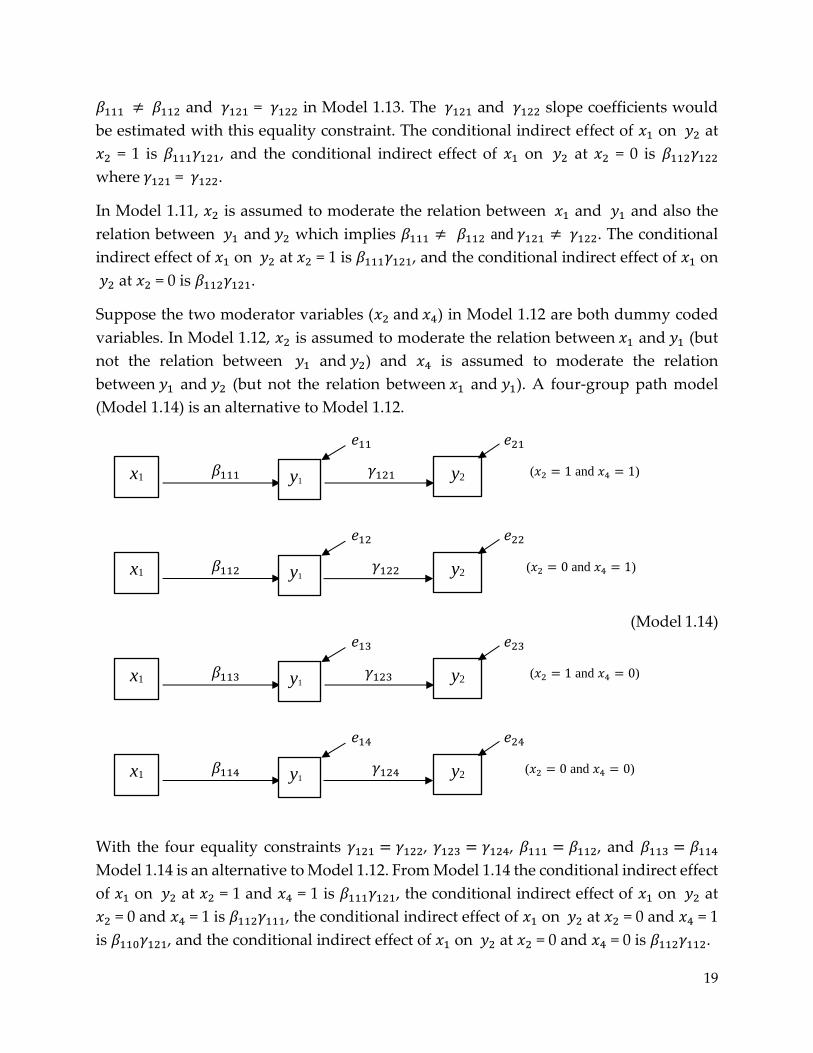
Suppose the two moderator variables (𝑥2 and 𝑥4) in Model 1.12 are both dummy coded

variables. In Model 1.12, 𝑥2 is assumed to moderate the relation between 𝑥1 and 𝑦1 (but

not the relation between 𝑦1 and 𝑦2) and 𝑥4 is assumed to moderate the relation

between 𝑦1 and 𝑦2 (but not the relation between 𝑥1 and 𝑦1). A four-group path model

(Model 1.14) is an alternative to Model 1.12.

𝑒11 𝑒21

𝛽111 𝛾121 (𝑥2 = 1 and 𝑥4 = 1)

𝑒12 𝑒22

𝛽112 𝛾122 (𝑥2 = 0 and 𝑥4 = 1)

(Model 1.14) 𝑒13 𝑒23

𝛽113 𝛾123 (𝑥2 = 1 and 𝑥4 = 0)

𝑒14 𝑒24

𝛽114 𝛾124 (𝑥2 = 0 and 𝑥4 = 0)

With the four equality constraints 𝛾121 = 𝛾122, 𝛾123 = 𝛾124, 𝛽111 = 𝛽112, and 𝛽113 = 𝛽114

Model 1.14 is an alternative to Model 1.12. From Model 1.14 the conditional indirect effect

of 𝑥1 on 𝑦2 at 𝑥2 = 1 and 𝑥4 = 1 is 𝛽111𝛾121, the conditional indirect effect of 𝑥1 on 𝑦2 at

𝑥2 = 0 and 𝑥4 = 1 is 𝛽112𝛾111, the conditional indirect effect of 𝑥1 on 𝑦2 at 𝑥2 = 0 and 𝑥4 = 1

is 𝛽110𝛾121, and the conditional indirect effect of 𝑥1 on 𝑦2 at 𝑥2 = 0 and 𝑥4 = 0 is 𝛽112𝛾112.

x1 y2 y11

y1

x1 y2 y11

y1

x1 y2 y11

y1

x1 y2 y11

y1

20

If Models 1.10, 1.11, and 1.12 are used with categorical moderator variables, the variances

of the two prediction errors (𝑒1 and 𝑒2) are assumed to be equal across the levels of each

moderator variable. Models 1.13 and 1.14 are more general and allow the prediction error

variances to vary across the levels of each moderator variables.

Multiple-group path models can be used with moderator variables that have more than

two categories. For example, if the moderator variable in Model 1.13 had three levels,

then Model 1.13 would have three groups.

The lavaan model specifications with defined conditional indirect effects are given below

for Models 1.13 and 1.14. In the first version of Model 1.13 (named model_13a), which is

an alternative to Model 1.10 when 𝑥2 has two categories, 𝑥2 is assumed to only moderate

the relation between 𝑥1 and 𝑦1. In the second version of Model 1.13 (named model_13b),

which is an alternative to Model 1.11 when 𝑥2 has two categories, 𝑥2 is assumed to

moderate the relation between 𝑥1 and 𝑦1 and the relation between 𝑦1 and 𝑦2. The ==

operator is used to imposes an equality constraint on a particular pair of slope

coefficients.

model_13a <- '

y1 ~ c(b111, b112)*x1

y2 ~ c(g121, g122)*y1

g121 == g122

conx1y2ind1 := b111*g12

conx1y2ind2 := b112*g12 '

fit <- sem(model_13a, data = mydata, fixed.x = F, group = "x2")

model_13b <- '

y1 ~ c(b111, b112)*x1

y2 ~ c(g121, g122)*y1


conx1y2ind2 := b112*g122 '

fit <- sem(model_13b, data = mydata, fixed.x = F, group = "x2")

model_14 <- '

y1 ~ c(b111, b112, b113, b114)*x1

y2 ~ c(g121, g122, g123, g124)*y1

g121 == g122

g123 == g124

b111 == b113

b112 == b114




conx1y2ind4 := b114*g124 '

fit <- sem(model_14, data = mydata, fixed.x = F, group = "x2")

21

1.10 Model Assessment in the GLM and MGLM

In the GLM and MGLM, every predictor variable is assumed to be related to every

response variable. These models can be assessed by examining the confidence intervals

for all slope coefficients, semipartial correlations, or standardized slope coefficients.

Confidence intervals for the squared multiple correlation of each response variable also

provides useful information. Suppose we believe that a population standardized slope

that is less than .2 in absolute value represents a weak or unimportant relation between

the predictor variable and the response variable, controlling for all other predictor

variables in the model. If a confidence interval for a population standardized slope is

completely outside the -.2 to .2 range, then we can conclude that the relation could be

important. If the confidence interval for the population standardized slope is completely

contained within the -.2 to .2 range, then we would conclude that the relation is weak or

unimportant. If the confidence interval for the population standardized slope includes

the values -.2 or .2, then the results are inconclusive. Inconclusive results should be

reported as such. Unstandardized slopes can be evaluated in the same way, but the

specification of a “small” value of an unstandardized slope depends on the scales of the

predictor variable and response variable. For instance, the slope coefficient for one

predictor variable might be considered small or unimportant if it with within the range -

15 to 15 while the slope coefficient for another predictor variable might be considered

small or unimportant if it is within the range -0.02 to 0.02.

Ideally, 95% Bonferroni confidence intervals for the population slope coefficients should

be computed. Consider a MGLM with s = 3 predictor variables and r = 2 response

variables which has six slope parameters. If the 95% Bonferroni confidence intervals for

all six standardized slopes are outside the -.2 to .2 range, then the researcher can be 95%

confident that all six population standardized slopes are greater than .2 in absolute value.

Or if three of the 95% Bonferroni confidence intervals for standardized slopes are outside

the -.2 to .2 range and three are within the -.2 to .2 range, the researcher can be 95%

confident that three of population standardized slopes are less than .2 in absolute value

and three of the other population standardized slopes are greater than .2 in absolute value.

MGLM programs will compute multivariate test statistics to test the null hypothesis

H0: B = 0 against the alternative hypothesis H1: B ≠ 0 where B is an s × r matrix of

population slope coefficients and 0 is an s × r matrix of zeros. Several multivariate test

statistics (Wilks’ lambda and Pallai’s trace are popular choices) can be used to H0: B = 0.

The null hypothesis H0: B = 0 states that every element in B is equal to zero and the

alternative hypothesis H1: B ≠ 0 states that at least one element in B is not equal to zero.

22

In the case of the MANOVA model, B = 0 indicates that for every response variable, the

population means are identical across all factor levels, and B ≠ 0 indicates that for at least

one response variable, there are least two population means that are not equal.

If the p-value for a particular multivariate test statistic is less than some small value (e.g.,

.05) the null hypothesis is rejected and the results are declared to be “significant”.

However, a statistical test that allows the researcher to simply decide if H0: B = 0 can or

cannot be rejected does not provide useful scientific information because the researcher

knows, before any data have been collected, that H0 is almost certainly false and hence

H1 is almost certainly true.

GLM programs can be used to test if any single column of B is equal to zero (with a

Bonferroni adjusted 𝛼-level of 𝛼/𝑟), but a multivariate test of H0: B = 0 is more likely to

produce a significant result, which explains its popularity. It is important to remember

that a significant result does not tell us which elements are nonzero, if they are positive

or negative, and how much they differ from zero. Furthermore, a nonsignificant result

does not imply B = 0.

1.11 Model Assessment in SUR and Path Models

Two sets of slope coefficients can be specified in a SUR model or a path model. One set

consists of all included paths, and a second set consists of all excluded paths. Let 𝜽1

represent the set of population slope coefficients that are included in the model, and let

𝜽2 represent the set of population slope coefficients that have been constrained to equal

zero (and their paths are omitted from the path diagram). To show that a SUR or path

model has been correctly specified, every slope coefficient in 𝜽1 should be meaningfully

large and every slope coefficient in 𝜽2 should be small or unimportant.

Suppose a population standardized slope that is less than .2 in absolute value is believed

to represent a small or unimportant relation between the predictor variable. Ideally, all

95% Bonferroni confidence intervals for the population standardized slopes in 𝜽1 will be

completely outside the -.2 to .2 range. If a confidence interval for a particular standardized

slope in 𝜽1 includes the value -.2 or .2, then the result is “inconclusive” and should be

reported as such.

Ideally, all 95% Bonferroni confidence intervals for the population standardized slopes

in 𝜽2 will be completely within the -.2 to .2 range. To assess the slope coefficients in 𝜽2,

the estimable omitted paths could be added to the model one at a time so that the

confidence interval for each standardized slope in 𝜽2 can be assessed. Unless the number

23

of parameters in 𝜽2 is small, it will be more convenient to examine the modification index

that can be computed for each excluded path. Each modification index is a one degree of

freedom chi-square test of the null hypothesis that the omitted path parameter is equal

to 0.

lavaan will compute a modification index for all excluded paths. The omitted path with

the largest modification index can be added to the model, and if the confidence interval

for the population standardized slope for this added path is completely contained with

the -.2 to .2 range, then it is likely that paths with smaller modification indices will also

have small standardized slopes and no further analyses will be required. If the confidence

interval for the omitted path when added to the model is completely outside the -.2 to .2

range and the inclusion of that path can be theoretically justified, that path could be

retained in the model. The omitted path with the next largest modification index would

then be examined. If a confidence interval for any standardized slope coefficient in 𝜽2

includes the values -.2 or .2, the result is “inconclusive” and should be reported as such.

Showing that all the slope coefficients in 𝜽1 are meaningfully large and all the slope

coefficients in 𝜽2 are small or unimportant would ideally be assessed using semipartial

correlations rather than standardized slopes. However, the current version of lavaan will

not compute confidence intervals for population semipartial correlations. The ci.spcor

R function can be used to compute a confidence interval for a semipartial correlation in

GLM, MGLM, and recursive path models. Although a standardized slope does not have

a simple interpretation (see section 2.12 of Part 2) in a model with multiple predictor

variables, a standardized slope simplifies to an interpretable Pearson correlation if there

is a single predictor of a particular variable. Also, a standardized slope is numerically

similar to a Pearson correlation if the predictors of a particular variable are weakly

correlated.

Although the above confidence interval approach provides useful information regarding

the magnitudes of both included and omitted path parameters, the traditional method of

assessing a SUR model or a path model involves a goodness-of-fit (GOF) test. A GOF test

is a test of the following null and alternative hypotheses regarding the excluded

parameters

H0: 𝜽2 = 0 H1: 𝜽2 ≠ 0

where 0 is a vector of zeros. In path models, not all excluded paths are estimable and 𝜽2

is assumed to be the set of omitted paths that are estimable.

24

A chi-square test statistic with degrees of freedom equal to the number of slope

coefficients in 𝜽2 can be used to test H0: 𝜽2 = 0. If the p-value for the chi-square statistic is

less than 𝛼 (usually .05), then H0 is rejected. A p-value greater than 𝛼 is traditionally (but

incorrectly) interpreted as evidence that the SUR model or path model is “correct” or

“provides a good fit to the data”. The GOF hypothesis testing procedure does not provide

useful scientific information. A failure to reject H0 does not imply that H0 is true or that

the model is “correct”. Furthermore, a rejection of H0 does not imply that all excluded

path parameters are meaningfully large. Remember that the p-value for the GOF test is

inversely related to the sample size with large sample sizes tending to give small p-values

even if all slope coefficients in 𝜽2 are small, and small sample sizes tending to give large

p-values even one or more slope coefficients in 𝜽2 are not small. However, if the sample

size is small and the p-value is small, that suggests that there could be one or more

omitted paths that might need to be added to the model.

Tests of the individual slope coefficients in 𝜽1 provide useful information about the

direction of a relation between two variables. The following test statistic can be computed

for each element in 𝜽1

z = 𝜃𝑗/𝑆𝐸�̂�𝑗 (1.5)

and can be used to decide if H0: 𝜃𝑗 = 0 can be rejected. If H0 is rejected, then the sign of 𝜃𝑗

will determine if H1: 𝜃𝑗 > 0 or H2: 𝜃𝑗 < 0 should be accepted. lavaan will compute z and its

corresponding p-value for every parameter in 𝜽1.

If only a few parameters are added or removed from the original model based on results

observed in the sample, the confidence intervals and p-values for all included paths

should not be adversely affected. However, if more than a few alterations to the original

model are made in an exploratory manner, the confidence intervals for the included slope

coefficients can be too narrow, the p-values for included slope coefficients can be too

small, and the p-value of the GOF test can be too large. All exploratory model

modifications should be reported along with a clear warning about potentially

misleading results.

1.12 Assumptions

Recall from Chapter 2 of Part 2 that the assumptions for hypothesis tests and confidence

intervals for an unstandardized slope in a GLM are: 1) random sampling, 2)

independence among participants, 3) linearity between the response variable and each

25

predictor variable (linearity assumption), 4) constant variability of the prediction errors

across the values of every predictor variable (equal prediction error variance assumption),

and 5) approximate normality of the prediction error in the study population (prediction

error normality assumption). The assumptions for hypothesis tests and confidence intervals

for each unstandardized slope in MGLM, SUR, or recursive path models are the same as

for a GLM.

In addition to the GLM assumptions, confidence intervals for squared multiple

correlations, semipartial correlations, Pearson correlations, and standardized slopes in

GLM, MGLM, SUR, or path models also assume that the set of all response and predictor

variables have an approximate multivariate normal distribution in the study population. A

multivariate normal distribution implies that each variable is normally distributed and

all pairs of variables are linearly related.

1.13 Missing Data

All of the hypothesis tests and confidence intervals described in this chapter assume that

every participant produces a score for all response variables and all predictor variables.

If a participant is missing any response variable or predictor variable score, lavaan will

eliminate that participant from the analysis. This approach to missing data is called

listwise deletion.

If the missing responses are MCAR (see Chapter 2 of Part 2), then the reduced sample

after listwise deletion remains a random sample from the original study population, and

inferential methods computed from the reduced sample will provide a description of the

original study population. One drawback of listwise deletion is that the sample size is

reduced and this leads to wider confidence intervals and less powerful tests. If the

missing data are assumed to be MCAR or MAR and approximate multivariate normality

of the observed variables can be assumed, then listwise deletion is not required and all

available data from all participants can be analyzed using a full information maximum

likelihood (FIML) estimation procedure. FIML can be requested in lavaan by including the

command missing = "fiml" within the sem function.

1.14 Assumption Diagnostics

Scatterplots of each response variable with each predictor variable are useful in assessing

the linearity assumption. Scatterplots of the residuals with each predictor variable (called

residual plots) are helpful in assessing the equal variance assumption. Skewness and

26

kurtosis estimates of the residuals are useful in assessing prediction error normality

assumption. Transforming the response variable (e.g., √𝑦, ln(y), 1/y) may reduce

prediction error non-normality.

To assess multivariate normality, assess the linearity and equal error variance

assumptions as described above. Also examine scatterplots for all pairs of predictor

variables to assess linearity for all pairs of predictor variables, and check all predictor

variables for skewness and kurtosis. Transforming one or more of the predictor variables

(e.g., √𝑥𝑗 , ln(𝑥𝑗), 1/𝑥𝑗) may reduce nonlinearity and non-normality of the predictor

variables. The multivariate normality assumption is not plausible in models with a

squared predictor variable (as in the quadratic model) or interaction terms.

In MGLM and recursive path models where hypothesis tests and confidence intervals for

each slope could be obtained from a GLM, the LAD estimates and confidence intervals

described in section 2.25 of Part 2 could be used if the prediction error normality or the

equal prediction error variance assumptions cannot be justified. If only the equal

prediction error variance assumption is a concern, the MacKinnon-White standard errors

(see section 2.28 of Part 2) can be used to obtain hypothesis tests and confidence intervals

for each slope coefficient in a MGML and recursive path model.

If the multivariate normality assumption for standardized slope confidence intervals

does not appear to be plausible, lavaan has an option to compute "robust" standard errors

do not assume multivariate normality. For example, the following command

fit <- sem(model, data = mydata, fixed.x = F, se = "robust")

will compute robust standard errors. Bootstrap standard errors (see section 2.26 of Part

2) also do not assume multivariate normality. The se = "bootstrap" command will

compute bootstrap standard errors.

It might seem that robust or bootstrap standard errors should always be used to compute

confidence intervals for standardized slopes or Pearson correlations because the

multivariate normality assumption is rarely justified and is very difficult to assess.

However, confidence intervals based on the robust or bootstrap standard errors can be

less accurate than the regular standard errors if the variables are only mildly nonnormal

and the sample size is small. When computing confidence intervals for standardized

slopes or Pearson correlations in the statistical models described in this chapter, the

recommendation here is to use the robust or bootstrap standard errors if the sample size

27

is at least 100 or if, regardless of sample size, there is clear evidence of large skewness or

kurtosis in the sample data that cannot be reduced using data transformations.

It also might seem that data transformations to reduce nonnormality are not needed with

robust or bootstrap standard errors. However, robust and bootstrap standard errors

require large sample sizes greater if the data are highly leptokurtic. A data transformation

that reduces leptokurtosis will allow a more effective use of robust or bootstrap standard

errors in smaller samples.

Even if all model assumptions are satisfied, hypothesis tests and confidence intervals for

indirect effects require a large sample size because the sampling distribution of a product

of parameter estimates can be highly nonnormal in small samples. Bootstrap confidence

intervals or Monte Carlo confidence intervals are recommended for standardized or

unstandardized indirect effects. Monte Carlo confidence intervals are recommended for

unstandardized indirect effects. Bootstrap confidence intervals can be requested in lavaan

but are computationally very slow. The Monte Carlo method is fast and performs about

as well as the bootstrap method for unstandardized indirect effects. The ci.indirect R

function will compute a Monte Carlo confidence interval for an indirect effect.

28

Key Terms

general linear model

confounding variable

multivariate general linear model

multivariate multiple regression model

MANOVA model

MANCOVA model

SUR model

path model

mediator variable

exogenous variable

endogenous variable

direct effect

indirect effect

total indirect effect

recursive model

nonrecursive model

conditional direct effect

conditional indirect effect

GOF test

modification index

Concept Questions

1. What is one way to control for confounding variables in a nonexperimental design?

2. How does a MGLM differ from a GLM?

3. Draw a path diagram (without y-intercepts) for a MGLM with q = 2 and r = 3 and

include the slope parameters.

4. What is the main difference between a MGLM and a SUR model?

5. What is the main difference between a SUR model and a path model?

6. Draw a path diagram (without y-intercepts) for a path model where 𝑥1 predicts 𝑦1 and

𝑦1 predicts 𝑦2 and include the slope parameters.

29

7. In a path model that predicts 𝑦1 from 𝑥1 and predicts 𝑦2 from 𝑦1, how is the indirect

effect of 𝑥1 on 𝑦2 defined?

8. How could you show that the population values of all included paths are meaningfully

large?

9. How could you show that the population values of all excluded paths in a SUR or path

model are small or unimportant?

10. What can one conclude if the test for H0: B* = 0 is “significant”?

11. What is the difference between a recursive path model and a nonrecursive path

model?

12. If there are a total of 6 variables (predictor variables plus response variables), what is

the maximum number of slope and covariance parameters that can be estimated?

13. Why are modification indices useful?

14. What are the assumptions for tests and confidence interval for unstandardized slope

coefficients in a GLM, MGLM, SUR model, or path model?

15. What are the assumptions for standardized slope confidence intervals?

16. Give the lavaan model specification for a GLM that predicts 𝑦1 from 𝑥1 and 𝑥2.

17. Give the lavaan model specification for a MGLM that predicts 𝑦1 and 𝑦2 from 𝑥1 and

𝑥2.

18. Give the lavaan model specification for a SUR model that predicts 𝑦1 from 𝑥1 and

predicts 𝑦2 from 𝑥1 and 𝑥2.

19. Give the lavaan model specification for a path model that predicts 𝑦1 from 𝑥1 and 𝑥2

and predicts 𝑦2 from 𝑦1.

20. Give the lavaan model specification for a path model that predicts 𝑦1 from 𝑥1 and

predicts 𝑦2 from 𝑦1. Include the specification for the indirect effect of 𝑥1 on 𝑦2.

30

Data Analysis Problems

1-1. Sixty male freshman and their fathers were randomly selected from a university

orientation for all 1,240 incoming male students. A trait aggression questionnaire

measured on a 0 to 100 scale was given to the sample of 60 male freshman and their

fathers. The sons also were asked to estimate the average number hours per week, during

their summer break, that they had played any type of violent video game. The researcher

believes that video game playing and father's aggression are predictors of the son's

aggression. The 214BHW1-1.sav file contains the sample data with variable names

sonaggr, fatheraggr and gamehrs.

a) Describe the study population.

b) What is the response variable and what are the two predictor variables in this study?

c) Compute 95% confidence intervals for the two population slope coefficients and

interpret the results.

d) Compute 95% confidence intervals for the two standardized population slope

coefficients and interpret the results.

e) Compute a 95% confidence interval for the population squared multiple correlation

and interpret this result.

f) Examine all pairwise scatterplots and check for nonlinearity or other problems.

31

1-2. One hundred and twenty students were randomly selected from a directory of about

5,200 freshman at UC Davis. The 120 students were paid to complete a social support

questionnaire and a college life satisfaction questionnaire. The following year, both

questionnaires were given to 105 of the original 120 students. The 214BHW1-2.sav file

contains the sample data with variable names SS1, CLS1, SS2, and CLS2.


b) In a SUR model with social support at year 1 (SS1) predicting college life satisfaction

at year 1 (CLS1) and social support at years 1 and 2 (SS1 and SS2) predicting college life

satisfaction at year 2 (CLS2), compute 95% confidence intervals for the three standardized

population slope coefficients and interpret the results.

c) Compute a 95% confidence interval for the population squared multiple correlation

for each response variable and interpret this result.

32

1-3 One hundred and fifty female students were randomly selected from the directories

of two San Jose high schools that contained the names and contact information for about

3,100 female students. Each participant was asked to report their mother’s years of

education and a description of their mother’s current job. The researcher assigned a 1 to

15 occupational status score to each job description. Each participant also answered an

educational goals questions that the researcher converted into years of education (e.g.,

“complete high school” = 12, “get a 2-year college degree” = 14, etc.). Each participant also

completed a 30-item achievement motivation questionnaire that was scored on a 30 to

210 scale. The 214BHW1-3.sav file contains the sample data with variable names

motherOC, motherED, AchMot, and EDgoal.


b) Draw a path diagram of a path model with motherED and motherOC predicting

AchMot and motherED and AchMot predicting EDgoal. The prediction errors for

AchMot and EDgoal are assumed to be uncorrelated.

c) Compute 95% confidence intervals for the four standardized population slope

coefficients and interpret the results.

d) Estimate the standardized indirect effects of motherOC and motherED on EDgoal.

Compute 95% confidence intervals for these two population standardized indirect effects

and interpret the results.

e) Estimate the standardized total effect of motherED on EDgoal. Compute a 95%

confidence interval for the population standardized total effect and interpret the results.

33

Chapter 2

Latent Factor Models

2.1 Measurement Error

Quantitative psychological attributes, such as "creativity", "resilience", or "neuroticism",

cannot be observed directly but are instead measured indirectly from responses to tests

or questionnaires. The difference between a person's true attribute value and a

measurement of the attribute is called measurement error as explained in Chapter 4 of

Part 1. All of the statistical models in Chapter 1 assume that all variables in the model are

devoid of measurement error.

Measurement error in a predictor variable can increase or decrease slope coefficients

depending on the correlations among the predictor variables and the amount of

measurement error in each predictor variable. Even if only one predictor variable is

measured with error, the slopes coefficients for other predictor variables also can be

affected. Measurement error in a response variable will increase the standard errors of

the slope estimates which results in wider confidence intervals and less powerful

hypothesis tests for the population slope coefficients. Measurement error in a mediator

variable can affect slope coefficients and standard errors.

If multiple measurements (from multiple test forms, multiple raters, multiple occasions,

multiple questionnaire items) of a predictor variable or response variable can be obtained,

then the latent factor models described in this chapter can be used to define the

unobservable attribute, called a latent factor, that is assumed to predict the values of the

observed measurements. In Chapter 3, the latent factor models in this chapter are

integrated into the statistical models of Chapter 1 to define a more general class of latent

variable statistical models that can be used to describe relations among latent factors. Latent

factors are devoid of certain types of measurement error, depending how the multiple

measurements are obtained, and then the latent variable statistical models will provide

more accurate estimates of slope coefficients and correlations.

2.2 Single-factor Model

If r measurements of the same attribute can be obtained from each participant, a single-

factor model for the jth measurement and a randomly selected participant is

34

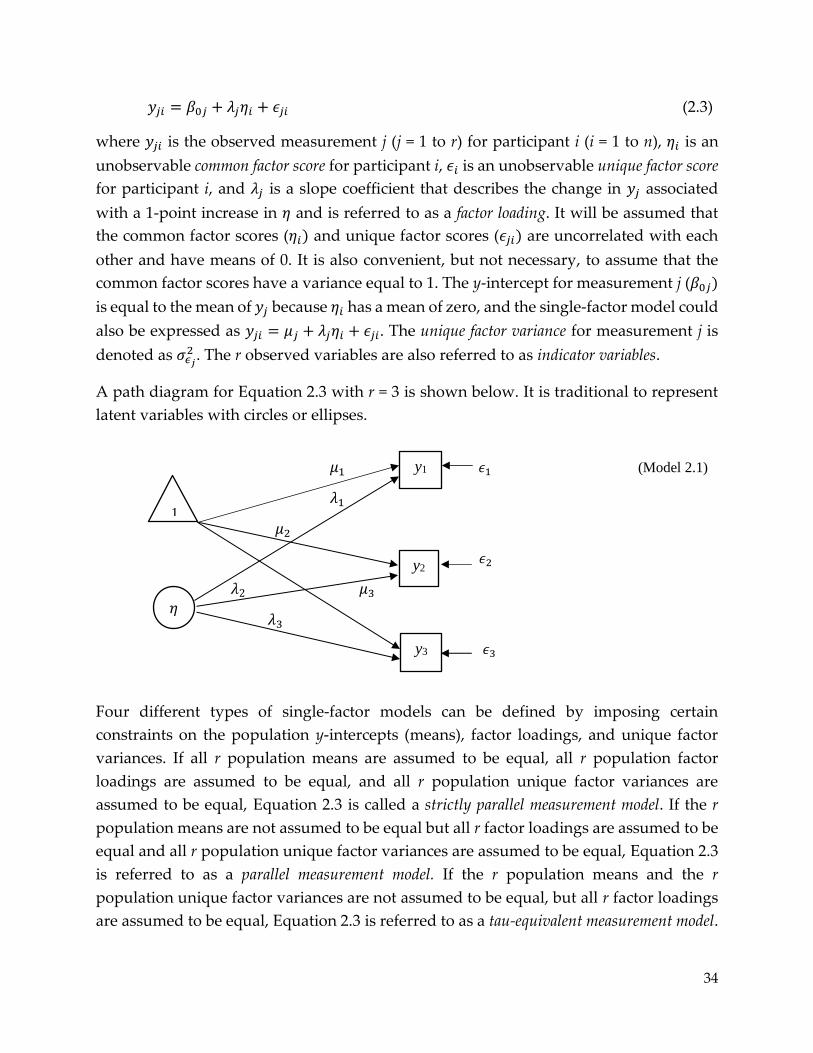
𝑦𝑗𝑖 = 𝛽0𝑗 + 𝜆𝑗𝜂𝑖 + 𝜖𝑗𝑖 (2.3)

where 𝑦𝑗𝑖 is the observed measurement j (j = 1 to r) for participant i (i = 1 to n), 𝜂𝑖 is an

unobservable common factor score for participant i, 𝜖𝑖 is an unobservable unique factor score

for participant i, and 𝜆𝑗 is a slope coefficient that describes the change in 𝑦𝑗 associated

with a 1-point increase in 𝜂 and is referred to as a factor loading. It will be assumed that

the common factor scores (𝜂𝑖) and unique factor scores (𝜖𝑗𝑖) are uncorrelated with each

other and have means of 0. It is also convenient, but not necessary, to assume that the

common factor scores have a variance equal to 1. The y-intercept for measurement j (𝛽0𝑗)

is equal to the mean of 𝑦𝑗 because 𝜂𝑖 has a mean of zero, and the single-factor model could

also be expressed as 𝑦𝑗𝑖 = 𝜇𝑗 + 𝜆𝑗𝜂𝑖 + 𝜖𝑗𝑖. The unique factor variance for measurement j is

denoted as 𝜎𝜖𝑗

2 . The r observed variables are also referred to as indicator variables.

A path diagram for Equation 2.3 with r = 3 is shown below. It is traditional to represent

latent variables with circles or ellipses.

𝜇1 𝜖1 (Model 2.1)

𝜆1

𝜇2

𝜖2

𝜆2 𝜇3

𝜆3

𝜖3

Four different types of single-factor models can be defined by imposing certain

constraints on the population y-intercepts (means), factor loadings, and unique factor

variances. If all r population means are assumed to be equal, all r population factor

loadings are assumed to be equal, and all r population unique factor variances are

assumed to be equal, Equation 2.3 is called a strictly parallel measurement model. If the r

population means are not assumed to be equal but all r factor loadings are assumed to be

equal and all r population unique factor variances are assumed to be equal, Equation 2.3

is referred to as a parallel measurement model. If the r population means and the r

population unique factor variances are not assumed to be equal, but all r factor loadings

are assumed to be equal, Equation 2.3 is referred to as a tau-equivalent measurement model.

y1

y2

y3

𝜂

1

35

If no constraints are imposed on the means, factor loadings, or unique factor variances,

Equation 2.3 is referred to as a congeneric measurement model.

In strictly parallel, parallel, and tau-equivalent measurement models where all factor

loadings are assumed to be equal, the 𝜆𝑗𝜂𝑖 component of Equation 2.3 simplifies to λ𝜂𝑖. In

these models, λ𝜂𝑖 is referred to as the true score for participant i, 𝜖𝑗𝑖 is the measurement error

for participant i and measurement j, and the unique factor variances 𝜎𝜖12 , 𝜎𝜖2

2 , … , 𝜎𝜖𝑟2 are

referred to as measurement error variances.

Strictly parallel measurements are important in applications where the r measurements

represent alternative forms of a test and a person’s test score is used for selection

purposes. Test developers for the GRE, SAT, driver’s exams, and other licensing exams

attempt to develop strictly parallel forms of a particular test. Strictly parallel forms of a

test are also useful in multiple group pretest-posttest designs with one form used at

pretest and the other form used at posttest. Parallel and tau-equivalent measurements are

useful in the latent variable statistical models of Chapter 3 to describe relations among

true scores.

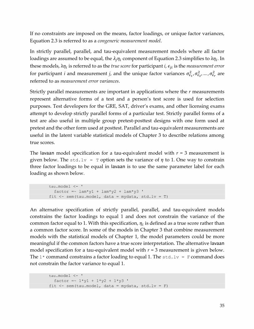
The lavaan model specification for a tau-equivalent model with r = 3 measurement is

given below. The std.lv = T option sets the variance of 𝜂 to 1. One way to constrain

three factor loadings to be equal in lavaan is to use the same parameter label for each

loading as shown below.

tau.model <- '

factor =~ lam*y1 + lam*y2 + lam*y3 '

fit <- sem(tau.model, data = mydata, std.lv = T)

An alternative specification of strictly parallel, parallel, and tau-equivalent models

constrains the factor loadings to equal 1 and does not constrain the variance of the

common factor equal to 1. With this specification, 𝜂𝑖 is defined as a true score rather than

a common factor score. In some of the models in Chapter 3 that combine measurement

models with the statistical models of Chapter 1, the model parameters could be more

meaningful if the common factors have a true score interpretation. The alternative lavaan

model specification for a tau-equivalent model with r = 3 measurement is given below.

The 1* command constrains a factor loading to equal 1. The std.lv = F command does

not constrain the factor variance to equal 1.

tau.model <- '

factor =~ 1*y1 + 1*y2 + 1*y3 '

fit <- sem(tau.model, data = mydata, std.lv = F)

36

An alternative specification of a congeneric model constrains a factor loading for one of

the observed variables (called the marker variable) to equal 1 and does not constrain the

variance of the common factor equal to 1. With this specification, the variance of the

common factor will equal the variance of the marker variable. The alternative lavaan

model specification for a congeneric model with r = 3 measurement is given below.

con.model <- '

factor =~ 1*y1 + y2 + y3 '

fit <- sem(con.model, data = mydata, std.lv = F)

2.3 General Latent Factor Model

In the single-factor model described above, each of the r observed variables (𝑦1, 𝑦2, … , 𝑦𝑟)

is predicted by a one factor. Now consider r observed variables that are each predicted

by q > 1 factors. The linear models for the r observed variables are given below.

𝑦1𝑖 = 𝜇1 + 𝜆11𝜂1𝑖 + 𝜆21𝜂2𝑖 + ⋯ + 𝜆𝑞1𝜂𝑞𝑖 + 𝜖1𝑖 (2.4a)

𝑦2𝑖 = 𝜇2 + 𝜆12𝜂1𝑖 + 𝜆22𝜂2𝑖 + ⋯ + 𝜆𝑞2𝜂𝑞𝑖 + 𝜖2𝑖

⋮

𝑦𝑟𝑖 = 𝜇𝑟 + 𝜆1𝑟𝜂1𝑖 + 𝜆2𝑟𝜂2𝑖 + ⋯ + 𝜆𝑞𝑟𝜂𝑞𝑖 + 𝜖𝑟𝑖

The r linear models define as general latent factor model. The general latent factor model

can be expressed in matrix notation as

Y = 𝟏𝝁 + 𝜼𝚲 + 𝐄 (2.4b)

where Y is an n × r matrix of r observed measurements for a random sample of n

participants, 𝟏 is a n × 1 vector of ones, 𝝁 is a 1 × r vector of population means of the r

measurements, 𝜼 is an n × q matrix of common factor scores for the n participants, 𝚲 is a

q × r matrix of factor loadings, and 𝐄 is an n × r matrix of unique factor scores. The

proportion of variance of 𝑦𝑗 that can be predicted by the q factors is

1 – 𝜎𝜖𝑗

2 /𝜎𝑦𝑗

2 (2.5)

and is called the communality of 𝑦𝑗. In strictly parallel, parallel, and tau-equivalent models

where 𝜎𝜖𝑗

2 represents measurement error variance, Equation 2.5 defines the reliability of

𝑦𝑗. Strictly parallel and parallel measurements are assumed to have equal measurement

error variances and hence they are equally reliable. Thus, the Spearman-Brown formulas

(see section 4.19 of Part 1) apply only to strictly parallel and parallel measurements.

37

The factor loadings might be difficult to interpret if the variances of the r indicator

variables are not similar and the scales of the indicator variables are not familiar to the

intended audience. When the variances of the indicators are unequal, the relative

magnitudes of the factor loadings do not describe the relative strengths of relations

between the factor and the indicator variables. A standardized factor loading is defined as

𝜆𝑗𝑘 = 𝜆𝑗𝑘(𝜎𝜂𝑗/𝜎𝑦𝑘

) which is analogous to how standardized slope coefficients are defined.

In factor analysis models with a single factor (i.e., measurement models) or with

uncorrelated factors, a standardized factor loading is equal to a Pearson correlation

between a factor and an indicator variable.

The correlations among the q factors are usually important parameters to estimate. The

correlations among the unique factors are usually assumed to equal 0. In some

applications, there is a theoretical justification for correlated unique factors and these

correlations can be included in the model. For instance, if 𝑦1 and 𝑦2 are self-report

measures and 𝑦3 and 𝑦4 are ratings from two different experts, we would expect a

positive correlation between 𝜖1 and 𝜖2 and a positive correlation between 𝜖3 and 𝜖4.

Not all of the parameters in a factor analysis model can be uniquely estimated and it is

necessary to impose some constraints on the model parameters to identify the model. A

factor analysis model in which some of its parameters are constrained is called a

confirmatory factor analysis (CFA) model. A necessary but not sufficient condition for the

parameters of a CFA to be identified is that that the number of estimated factor loadings,

factor variances, unique factor variances, unique factor correlations, and factor

correlations must be less than r(r + 1)/2. Sufficient conditions for CFA model identification

are more complicated. The following strategy will usually work: set all factor variances

to 1, set all unique factor correlations to 0, and set at least one factor loading from each

factor to 0. Also, if a factor predicts only two observed variables, then those two factor

loadings should be equality constrained.

For certain models that will be considered in Chapter 3, some of the factors will be treated

as predictor variables and some of the factors will be treated as response variables. The

variances of the predictor variable factors can be set at 1, but if the variance of a response

variable factor needs to be estimated, then one factor loading can be set to 1 to identify

the model. When one of the factor loadings is set to 1, the variance of that factor will then

equal the variance of the observed variable that has the loading of 1. In strictly parallel,

parallel, and tau-equivalent models, all factor loadings would be set equal to 1 if the factor

variance is to be estimated.

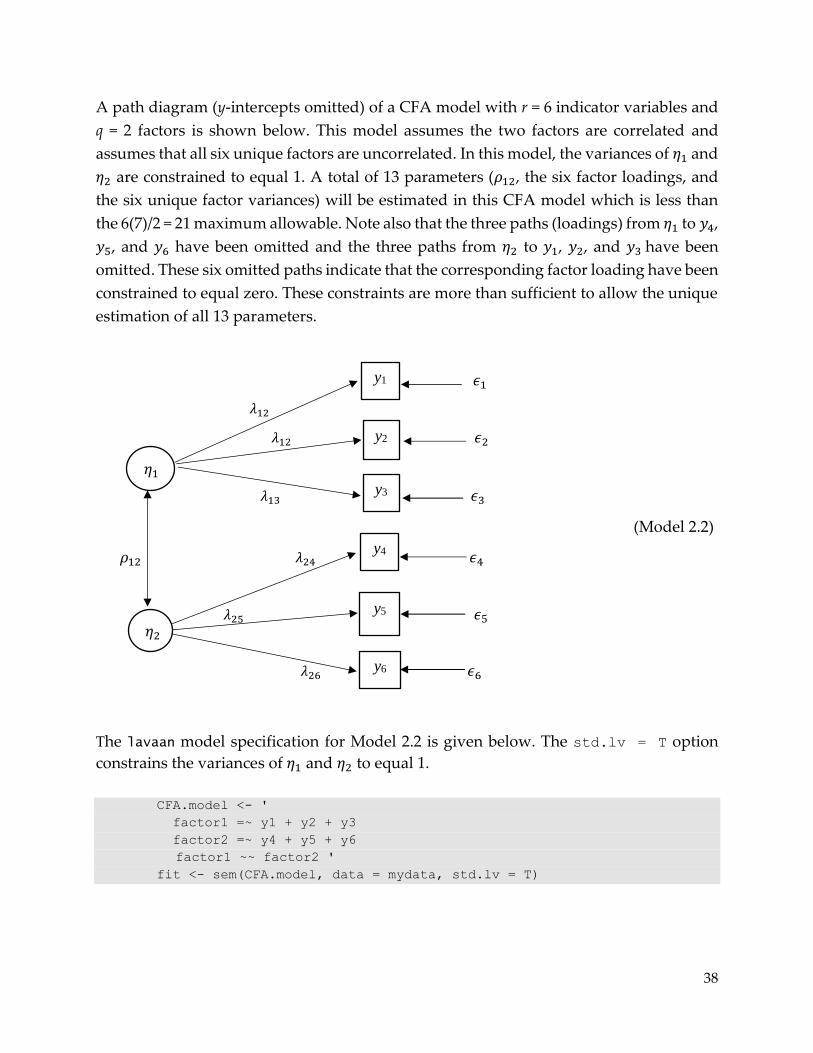
38

A path diagram (y-intercepts omitted) of a CFA model with r = 6 indicator variables and

q = 2 factors is shown below. This model assumes the two factors are correlated and

assumes that all six unique factors are uncorrelated. In this model, the variances of 𝜂1 and

𝜂2 are constrained to equal 1. A total of 13 parameters (𝜌12, the six factor loadings, and

the six unique factor variances) will be estimated in this CFA model which is less than

the 6(7)/2 = 21 maximum allowable. Note also that the three paths (loadings) from 𝜂1 to 𝑦4,

𝑦5, and 𝑦6 have been omitted and the three paths from 𝜂2 to 𝑦1, 𝑦2, and 𝑦3 have been

omitted. These six omitted paths indicate that the corresponding factor loading have been

constrained to equal zero. These constraints are more than sufficient to allow the unique

estimation of all 13 parameters.

E 𝜖1

𝜆12

𝜆12 𝜖2

𝜆13 𝜖3

(Model 2.2)

𝜌12 𝜆24 𝜖4

𝜆25 𝜖5

𝜆26 𝜖6

The lavaan model specification for Model 2.2 is given below. The std.lv = T option

constrains the variances of 𝜂1 and 𝜂2 to equal 1.

CFA.model <- '

factor1 =~ y1 + y2 + y3

factor2 =~ y4 + y5 + y6

factor1 ~~ factor2 '

fit <- sem(CFA.model, data = mydata, std.lv = T)

𝜂2

y5

y1

y3

y4

𝜂1

y2

y6

39

2.4 Exploratory Factor Analysis

A factor analysis model in which every factor predicts every observed variable and the

unique factors are all uncorrelated is called an exploratory factor analysis (EFA) model. The

EFA model is traditionally used in applications where the researcher is trying to discover

and understand the underlying factor structure of r observed variables. In an EFA model,

the factor loadings cannot be uniquely estimated. With an infinite number of possible

factor loading estimates, EFA programs allow the user to rotate the factor loadings to

make them more easily interpreted. The rotation algorithms search for a simple structure

in which each indicator variable ideally has a large path from only one factor and small

paths from all other factors. If the factors are assumed to be uncorrelated, orthogonal

rotation methods are used, and the varimax method is the most popular orthogonal

rotation method. With correlated factors assumed, oblique rotation methods are used. The

direct oblimin and promax methods are the popular oblique rotation methods. An oblique

rotation will usually produce a more interpretable simple structure of factor loadings

than an orthogonal rotation. However, it could be difficult to interpret the meaning of the

factors if they are highly correlated. EFA programs allow the user to specify the number

of factors. If two or more factors are highly correlated, a more interpretable result might

be obtained by reducing the number of factors in the EFA model.

With an orthogonal rotation, EFA programs will produce an r x q structure matrix of

estimated Pearson correlations between the r observed variables and the q factors. With

an oblique rotation, EFA programs will produce a structure matrix and an r x q

standardized or unstandardized pattern matrix that contains estimated standardized or

unstandardized factor loadings. With an oblique rotation, some EFA programs provide

an option to compute a reference structure matrix which is a matrix of semipartial

correlations between each variable and each factor controlling for the other factors. With

oblique rotation, an examination of both the structure matrix and the pattern matrix (or

reference structure matrix) helps to better understand the nature of the factors.

EFA programs give the user an option to factor analyze either the correlations or the

covariances among the r variables. An analysis of correlations is recommended in most

EFA applications. EFA programs allow the user to specify the number of factors, but the

researcher often does not know how many factors to specify. EFA programs can produce

a scree plot of the eigenvalues. The eigenvalue for each factor is equal to the sum of the

squared Pearson correlations between that factor and each of the r variables.

The optimal number of factors is often at or to the left of the point where the scree plot

straightens out. The scree plot below suggests that two or three factors might be a good

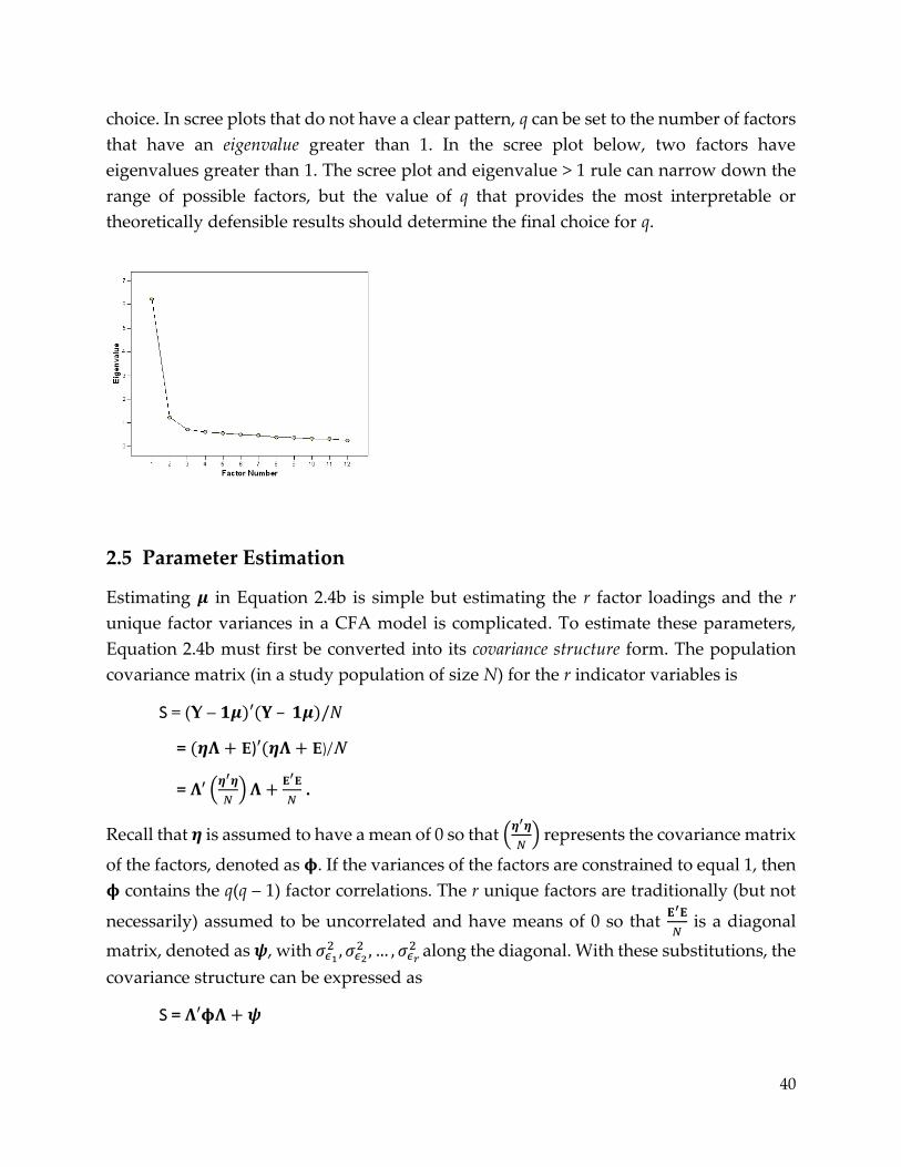
40

choice. In scree plots that do not have a clear pattern, q can be set to the number of factors

that have an eigenvalue greater than 1. In the scree plot below, two factors have

eigenvalues greater than 1. The scree plot and eigenvalue > 1 rule can narrow down the

range of possible factors, but the value of q that provides the most interpretable or

theoretically defensible results should determine the final choice for q.

2.5 Parameter Estimation

Estimating 𝝁 in Equation 2.4b is simple but estimating the r factor loadings and the r

unique factor variances in a CFA model is complicated. To estimate these parameters,

Equation 2.4b must first be converted into its covariance structure form. The population

covariance matrix (in a study population of size N) for the r indicator variables is

S = (Y – 𝟏𝝁)′(𝐘 – 𝟏𝝁)/𝑁

= (𝜼𝚲 + E)′(𝜼𝚲 + E)/N

= 𝚲′ (𝜼′𝜼

𝑁) 𝚲 +

𝐄′𝐄

𝑁 .

Recall that 𝜼 is assumed to have a mean of 0 so that (𝜼′𝜼

𝑁) represents the covariance matrix

of the factors, denoted as 𝛟. If the variances of the factors are constrained to equal 1, then

𝛟 contains the q(q – 1) factor correlations. The r unique factors are traditionally (but not

necessarily) assumed to be uncorrelated and have means of 0 so that 𝐄′𝐄

𝑁 is a diagonal

matrix, denoted as 𝝍, with 𝜎𝜖12 , 𝜎𝜖2

2 , … , 𝜎𝜖𝑟 2 along the diagonal. With these substitutions, the

covariance structure can be expressed as

S = 𝚲′𝛟𝚲 + 𝝍

41

and the goal is to find estimates of 𝚲 , 𝛟, and 𝝍, denoted as �̂�, �̂�, and �̂�, such that

�̂� = �̂�′�̂��̂� + �̂� is the closest possible approximation to the estimated covariance matrix

�̂� = (Y – 𝟏�̂�)′(𝐘 – 𝟏�̂�)/(𝑛 − 1).

The following goodness of fit function can be used to quantify how well �̂� approximates �̂�.

T = tr[{(�̂� – �̂�)𝐖}2](𝑛 − 1)/2 . (2.6)

The estimates of 𝝀, 𝛟 and 𝝍 that minimize T are called maximum likelihood (ML) estimates

if W is set to �̂�−𝟏. The estimates are called generalized least squares (GLS) estimates if W is

set to �̂�−𝟏 and are called unweighted least squares (ULS) estimates if W is set to I. With ML

and GLS estimation, T has an approximate chi-square distribution and can be used to test

hypotheses as will be explained later. Most textbooks omit the (n – 1) term from Equation

2.6 and then explain that n – 1 times the fit function has a chi-square distribution.

Compared to GLS estimates, ML estimates tend to be less biased in small samples, and

compared to ULS estimates, ML estimates have smaller standard errors. Although T is

not chi-squared distributed with ULS estimation, the ULS estimates can be less biased

and have sampling distributions that more closely approximate a normal distribution

than ML and GLS estimates in small samples.

Solving for the values of �̂� , �̂�, and �̂� that minimize Equation 2.6 is computationally

difficult. To minimize T, the fit function is first computed using starting values for �̂�,

�̂�, and �̂�, and then the values of �̂�, �̂�, and �̂� are systematically varied (subject to any

constraints on the parameter values) until the fit function appears to have reached a

minimum value. ML, GLS, and ULS estimates of 𝝀, 𝛟 and 𝝍 can be obtained in lavaan

(ML is the default method). lavaan also will compute standard errors of the parameter

estimates that can be used to compute confidence intervals for the population factor

loadings, correlations among factors, and unique factor variances.

In EFA models, parameter estimation is called “extraction”. The principal axis method of

extraction is a very old method that is still commonly used in EFA applications. The

principle axis method remains popular because it is faster than the ML method and

sometimes is able to produce parameter estimates in situations where the fit function

(Equation 2.6) will not converge to a minimum value.

42

2.6 Confidence Intervals for Factor Loadings and Unique Factor Variances

An approximate 100(1 – 𝛼)% confidence interval for 𝜆𝑗𝑘 is

�̂�𝑗𝑘 ± 𝑧𝛼/2𝑆𝐸�̂�𝑗𝑘 (2.7)

and an approximate 100(1 – 𝛼)% confidence interval for a difference between any two

factor loadings (e.g., 𝜆11 and 𝜆21) is

�̂�11 − �̂�21 ± 𝑧𝛼/2√𝑣𝑎𝑟(�̂�11) + 𝑣𝑎𝑟(�̂�21) − 2𝑐𝑜𝑣(�̂�11, �̂�21) . (2.8)

Using the := operator, lavaan can compute Formula 2.8 for unstandardized or

standardized factor loadings.

An approximate 100(1 – 𝛼)% confidence interval for the ratio of any two measurement

error variances (e.g., 𝜎𝜖12 and 𝜎𝜖2

2 ) could be used to assess the feasibility of a parallel or

strictly parallel model

exp[𝑙𝑛 (�̂�𝜖1

2

�̂�𝜖22 ) ± 𝑧𝛼/2√

𝑣𝑎𝑟(�̂�𝜖12 )

�̂�𝜖14 +

𝑣𝑎𝑟(�̂�𝜖22 )

�̂�𝜖24 −

2𝑐𝑜𝑣(�̂�𝜖12 , �̂�𝜖2

2 )

�̂�𝜖12 �̂�𝜖2

2 ]. (2.9)

Using the := operator, lavaan can compute a confidence interval for 𝑙𝑛(𝜎𝜖12 /𝜎𝜖2

2 ) which

can be exponentiated by hand to obtain Formula 2.9.

When examining all pairwise differences in factor loadings or all pairwise ratios of

unique factor variances in a congeneric model, replacing 𝛼 with 𝛼∗ = 𝛼/𝑣 in Formulas 2.8

and 2.9, where v = r(r – 1)/2, gives a set of simultaneous Bonferroni confidence intervals.

The square-roots of the endpoints of Formula 2.9 gives a confidence interval for standard

deviations that are easier to interpret than variances.

If all pairwise comparisons of factor loadings suggest that the 𝜆𝑗 values are similar, that

would support the use of a tau-equivalent model; and additionally, if all pairwise

comparisons of measurement error variances suggest that the 𝜎𝑒𝑗

2 values are similar, that

would support the use of a parallel measurement model. If the parallel model

assumptions appear to be reasonable, confidence intervals for all pairwise differences in

means can be computed to determine if a strictly parallel model is reasonable. Unless r is

small, reporting all r(r – 1)/2 pairwise comparisons can become unwieldy. It may suffice

to simply report �̂�𝑚𝑎𝑥 − �̂�𝑚𝑖𝑛, √�̂�𝜖𝑚𝑎𝑥2 /�̂�𝜖𝑚𝑖𝑛

2 , and �̂�𝑚𝑎𝑥 − �̂�𝑚𝑖𝑛 along with their Bonferroni

confidence intervals. The following lavaan model specification defines all pairwise

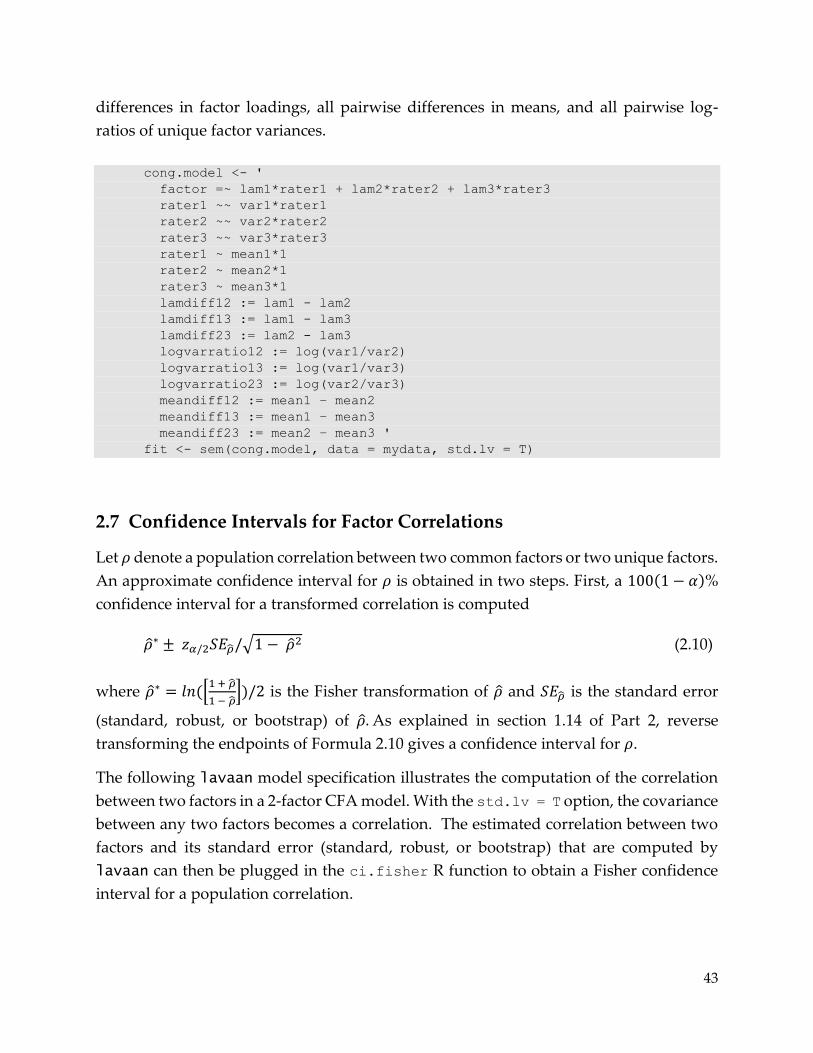
43

differences in factor loadings, all pairwise differences in means, and all pairwise log-

ratios of unique factor variances.

cong.model <- '

factor =~ lam1*rater1 + lam2*rater2 + lam3*rater3

rater1 ~~ var1*rater1



rater1 ~ mean1*1

rater2 ~ mean2*1

rater3 ~ mean3*1

lamdiff12 := lam1 - lam2



logvarratio12 := log(var1/var2)



meandiff12 := mean1 – mean2

meandiff13 := mean1 – mean3

meandiff23 := mean2 – mean3 '

fit <- sem(cong.model, data = mydata, std.lv = T)

2.7 Confidence Intervals for Factor Correlations

Let 𝜌 denote a population correlation between two common factors or two unique factors.

An approximate confidence interval for 𝜌 is obtained in two steps. First, a 100(1 − 𝛼)%

confidence interval for a transformed correlation is computed

�̂�∗ ± 𝑧𝛼/2𝑆𝐸�̂�/√1 − �̂�2 (2.10)

where �̂�∗ = 𝑙𝑛 ([1 + �̂�

1 − �̂�])/2 is the Fisher transformation of �̂� and 𝑆𝐸�̂� is the standard error

(standard, robust, or bootstrap) of �̂�. As explained in section 1.14 of Part 2, reverse

transforming the endpoints of Formula 2.10 gives a confidence interval for 𝜌.

The following lavaan model specification illustrates the computation of the correlation

between two factors in a 2-factor CFA model. With the std.lv = T option, the covariance

between any two factors becomes a correlation. The estimated correlation between two

factors and its standard error (standard, robust, or bootstrap) that are computed by

lavaan can then be plugged in the ci.fisher R function to obtain a Fisher confidence

interval for a population correlation.

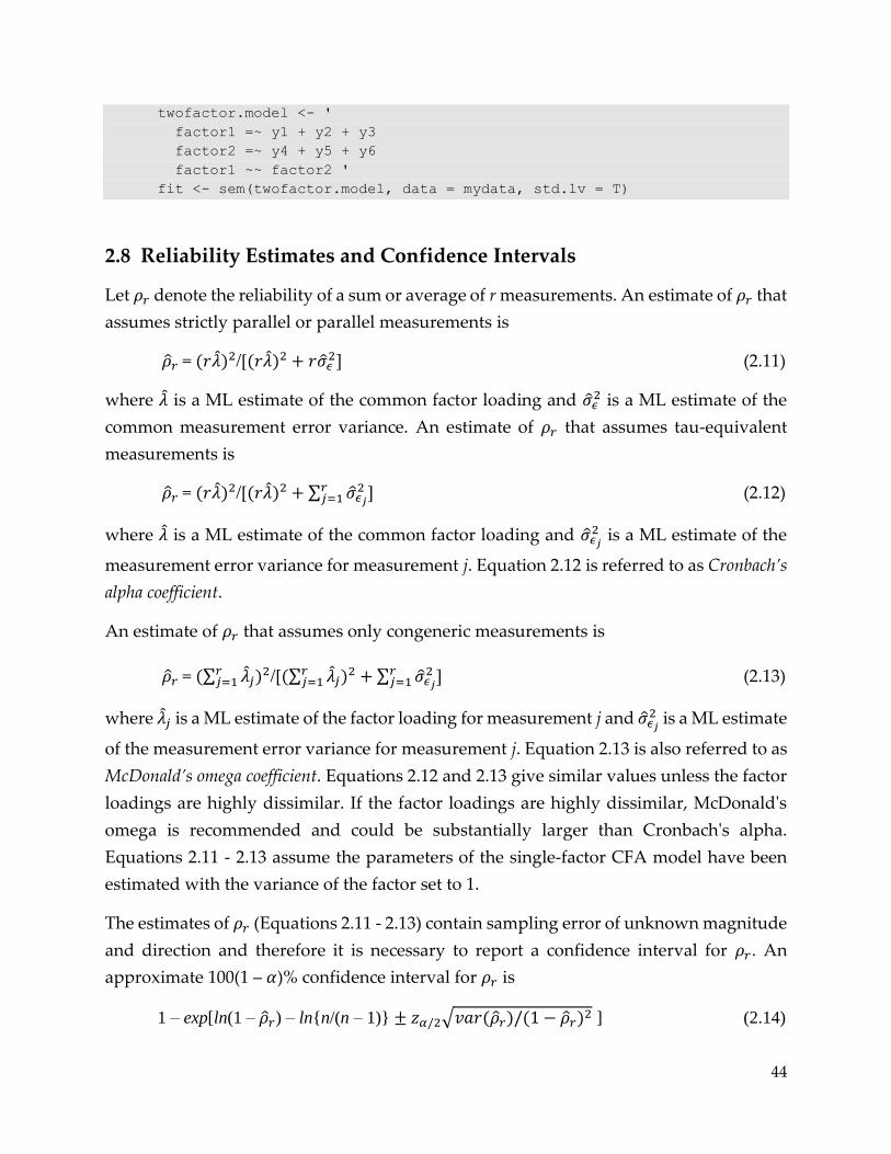
44

twofactor.model <- '

factor1 =~ y1 + y2 + y3

factor2 =~ y4 + y5 + y6

factor1 ~~ factor2 '

fit <- sem(twofactor.model, data = mydata, std.lv = T)

2.8 Reliability Estimates and Confidence Intervals

Let 𝜌𝑟 denote the reliability of a sum or average of r measurements. An estimate of 𝜌𝑟 that

assumes strictly parallel or parallel measurements is

�̂�𝑟 = (𝑟�̂�)2/[(𝑟�̂�)2 + 𝑟�̂�𝜖2] (2.11)

where �̂� is a ML estimate of the common factor loading and �̂�𝜖2 is a ML estimate of the

common measurement error variance. An estimate of 𝜌𝑟 that assumes tau-equivalent

measurements is

�̂�𝑟 = (𝑟�̂�)2/[(𝑟�̂�)2 + ∑ �̂�𝜖𝑗

2𝑟𝑗=1 ] (2.12)

where �̂� is a ML estimate of the common factor loading and �̂�𝜖𝑗

2 is a ML estimate of the

measurement error variance for measurement j. Equation 2.12 is referred to as Cronbach’s

alpha coefficient.

An estimate of 𝜌𝑟 that assumes only congeneric measurements is

�̂�𝑟 = (∑ �̂�𝑗𝑟𝑗=1 )2/[(∑ �̂�𝑗

𝑟𝑗=1 )2 + ∑ �̂�𝜖𝑗

2𝑟𝑗=1 ] (2.13)

where �̂�𝑗 is a ML estimate of the factor loading for measurement j and �̂�𝜖𝑗

2 is a ML estimate

of the measurement error variance for measurement j. Equation 2.13 is also referred to as

McDonald’s omega coefficient. Equations 2.12 and 2.13 give similar values unless the factor

loadings are highly dissimilar. If the factor loadings are highly dissimilar, McDonald's

omega is recommended and could be substantially larger than Cronbach's alpha.

Equations 2.11 - 2.13 assume the parameters of the single-factor CFA model have been

estimated with the variance of the factor set to 1.

The estimates of 𝜌𝑟 (Equations 2.11 - 2.13) contain sampling error of unknown magnitude

and direction and therefore it is necessary to report a confidence interval for 𝜌𝑟. An

approximate 100(1 – 𝛼)% confidence interval for 𝜌𝑟 is

1 – exp[ln(1 – �̂�𝑟) – ln{n/(n – 1)} ± 𝑧𝛼/2√𝑣𝑎𝑟(�̂�𝑟)/(1 − �̂�𝑟)2 ] (2.14)

45

where ln{n/(n – 1)} is a bias adjustment and 𝑣𝑎𝑟(�̂�𝑟) is the squared standard error of �̂�𝑟 .

The ci.reliablity R function will compute Formula 2.14 for any of the reliability

estimates given in Equations 2.11 - 2.13 using the estimate and standard error (standard,

robust, or bootstrap) computed in lavaan. Assuming r parallel measurements, the

ci.cronbach.par R function will compute an exact confidence interval for Cronbach's

alpha using only an estimate of Cronbach's alpha. Cronbach's alpha assumes tau-

equivalent measurements but the exact confidence interval for Cronbach's alpha make a

stronger assumption of parallel measurements.

When the multiple measurements are different forms of a test or different raters, the

reliability of a single form or a single rater could be of interest. Assuming strictly parallel

or parallel measurements, a confidence interval for 𝜌𝑟 can be transformed into a

confidence interval for the reliability of a single measurement using the Spearman-Brown

formulas in section 4.18 of Part 1.

The lavaan model specification for a parallel measurement model for three raters is given

below.

par.model <- '

true =~ lam*rater1 + lam*rater2 + lam*rater3

rater1 ~~ var*rater1



rel := (3*lam)^2/((3*lam)^2 + 3*var) '

fit <- sem(par.model, data = mydata, std.lv = T)

A common label is used to equality-constrain the three factor loadings and the three error

variances. The rel := (3*lam)^2/((3*lam)^2 + 3*var) command defines a new

parameter that is the reliability of the sum (or average) of the r = 3 parallel measurements.

A tau-equivalent measurement model can be specified using the following code where

different labels are used for each error variance.

tau.model <- '

true =~ lam*rater1 + lam*rater2 + lam*rater3




alpha := (3*lam)^2/((3*lam)^2 + var1+var2+var3) '

46


A congeneric measurement model is specified below by using different labels for the

factor loadings and different labels for the unique variances. Alternatively, the optional

parameters labels could be omitted and the parameters would be estimated without

equality constraints.

cong.model <- '





omega := (lam1+lam2+lam3)^2/((lam1+lam2+lam3)^2 + var1+var2+var3) '


2.9 Second-order CFA Model

There are q(q – 1)/2 correlations among the q factors in a multi-factor CFA model that can

be estimated. It might be possible to adequately represent these correlations by a second-

order factor. In a second-order CFA model, the q factors are called first-order factors and

serve as indicators of a second-order factor. Suppose there are q = 5 first-order factors that

represent different aspects of a common attribute. This common attribute is referred to

as a general factor, and we would expect the 5(4)/2 = 10 correlations among the five first-

order factors to be moderately large. If this is the case, then the ten correlations among

the five first-order factors could be described more parsimoniously using a second-order

factor that requires the estimation of only five second-order factor loadings. A path

diagram of a second-order CFA with two first-order factors is shown below (Model 2.3).

In this example, the two second-order factor loadings are equality constrained and the

variances of each factors is set to 1.

The first-order factors in a second-order CFA can be viewed as mediator variables.

Suppose the second-order factor in Model 2.3 is assumed to be "Character Strength" is

believed to predict the first-order factors of "Integrity" and "Temperance". The Integrity

first-order factor is believed to predict the responses on three Integrity questionnaire

items, and the Temperance first-order factor is believed to predict the responses on three

Temperance questionnaire items. In this example, the Integrity and Temperance factors

mediate the relation between the Character Strength factor and the questionnaire items.

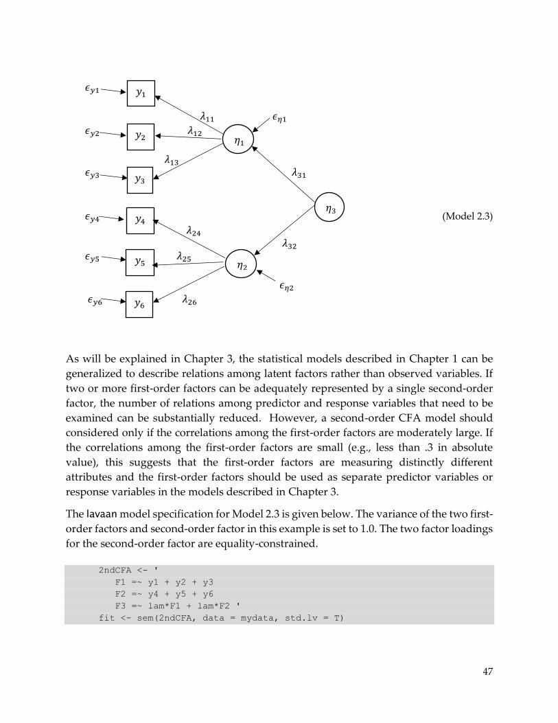
47

𝜖𝑦1

𝜆11 𝜖𝜂1

𝜖𝑦2 𝜆12

𝜆13 𝜖𝑦3 𝜆31

𝜖𝑦4 (Model 2.3)

𝜆24 𝜆32 𝜖𝑦5 𝜆25

𝜖𝜂2

𝜖𝑦6 𝜆26

As will be explained in Chapter 3, the statistical models described in Chapter 1 can be

generalized to describe relations among latent factors rather than observed variables. If

two or more first-order factors can be adequately represented by a single second-order

factor, the number of relations among predictor and response variables that need to be

examined can be substantially reduced. However, a second-order CFA model should

considered only if the correlations among the first-order factors are moderately large. If

the correlations among the first-order factors are small (e.g., less than .3 in absolute

value), this suggests that the first-order factors are measuring distinctly different

attributes and the first-order factors should be used as separate predictor variables or

response variables in the models described in Chapter 3.

The lavaan model specification for Model 2.3 is given below. The variance of the two first-

order factors and second-order factor in this example is set to 1.0. The two factor loadings

for the second-order factor are equality-constrained.

2ndCFA <- '

F1 =~ y1 + y2 + y3

F2 =~ y4 + y5 + y6

F3 =~ lam*F1 + lam*F2 '

fit <- sem(2ndCFA, data = mydata, std.lv = T)

𝑦1

𝑦2

𝑦3

𝑦4

𝑦5

𝑦6

𝜂1

𝜂2

𝜂3

48

2.10 Bifactor CFA Model

A bifactor CFA model is an alternative to a congeneric measurement model where certain

subsets of unique factors are assumed to be correlated. Correlated unique factor scores

occur when different subsets of indicator variables are measured using different

methods. For example, suppose three indicator variables are self-report measures of three

aspects of job performance and three other indicator variables are overall job performance

ratings from three coworkers. Some participants will overstate their performance while

other employees will understate their performance and this will introduce a correlation

among the three self-report measures.

A bifactor model has one general factor that predicts all of the indicator variables plus

one or more specific factors that predict a subset of the indicator variables. Any subset of

indicator variables that are assumed to have correlated unique factor scores can be

predicted by a specific factor. If four or more indicator variables have correlated unique

factors, including a specific factor to predict those variables is more parsimonious than

specifying all the covariances among the unique factors. For example, with four

correlated unique factors, there are 4(3)/2 = 6 covariances that would need to be estimated,

but it is possible that these covariances could be adequately represented by a single

specific factor where only four factor loadings need to be estimated.

With uncorrelated general and specific factors, the standardized factor loadings in the

bifactor CFA are equal to correlations between a factor and an indicator variable. The

standardized factor loadings for the general factor should be substantially larger than the

standardized factor loadings for the specific factors. If the standardized factor loadings

for a particular specific factor are large, this suggests that this specific factor could be

substantively interesting and it might be more appropriate to use a multi-factor CFA

model that includes only the specific factors (which can be correlated) and excludes the

general factor.

A path diagram of a bifactor CFA model is shown below (Model 2.4) where 𝜂3 is the

general factor and 𝜂1 and 𝜂2 are the specific factors. In this example, the variances of the

general factor and the two specific factors are set to 1. The factor loadings for the specific

factors in Model 2.4 have not been equality constrained. In applications where the

indicators of each specific factor are tau-equivalent, it would be appropriate to equality

constrain the factor loadings for each specific factor (e.g., 𝜆11 = 𝜆12 = 𝜆13 and 𝜆24 =

𝜆25 = 𝜆26.

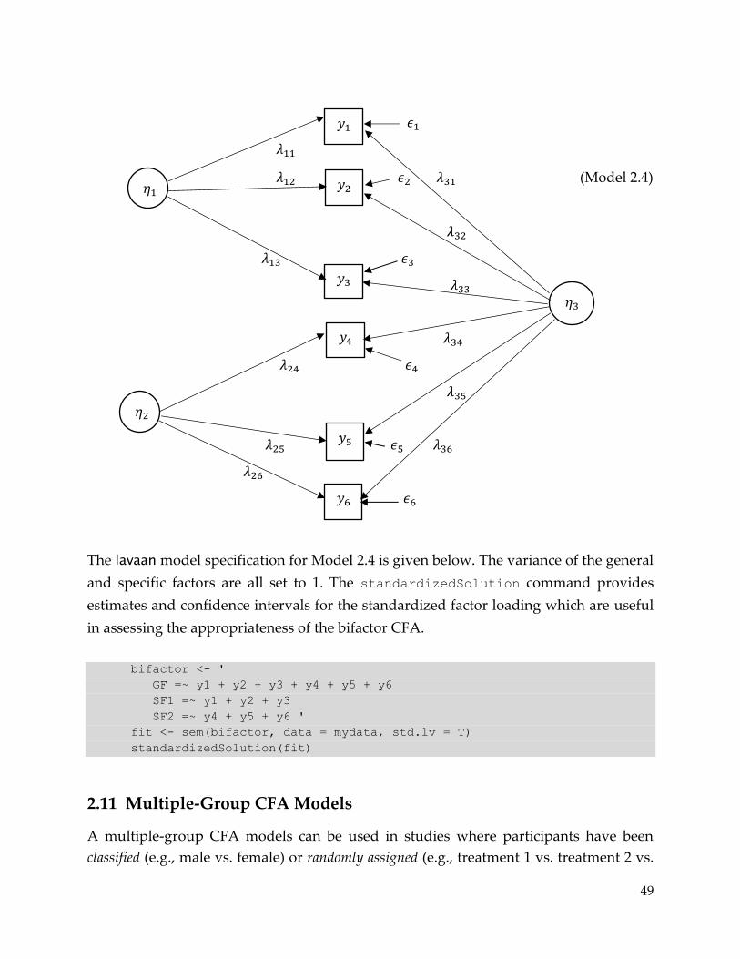
49

𝜖1

𝜆11

𝜆12 𝜖2 𝜆31 (Model 2.4)

𝜆32

𝜆13 𝜖3

𝜆33

𝜆34

𝜆24 𝜖4

𝜆35

𝜆25 𝜖5 𝜆36

𝜆26

𝜖6

The lavaan model specification for Model 2.4 is given below. The variance of the general

and specific factors are all set to 1. The standardizedSolution command provides

estimates and confidence intervals for the standardized factor loading which are useful

in assessing the appropriateness of the bifactor CFA.

bifactor <- '

GF =~ y1 + y2 + y3 + y4 + y5 + y6

SF1 =~ y1 + y2 + y3

SF2 =~ y4 + y5 + y6 '

fit <- sem(bifactor, data = mydata, std.lv = T)


2.11 Multiple-Group CFA Models

A multiple-group CFA models can be used in studies where participants have been

classified (e.g., male vs. female) or randomly assigned (e.g., treatment 1 vs. treatment 2 vs.

𝜂2

𝑦5

𝑦1

𝑦3

𝑦4

𝑦6

𝜂1𝑦2

𝜂3

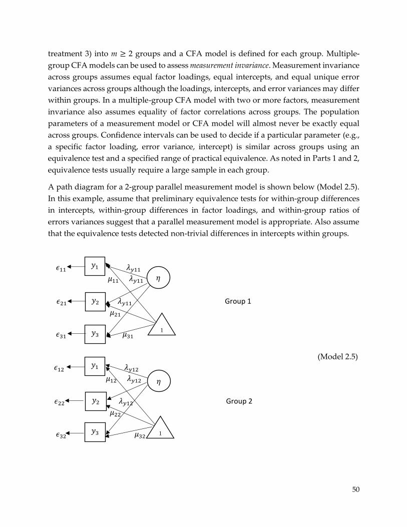
50

treatment 3) into m ≥ 2 groups and a CFA model is defined for each group. Multiple-

group CFA models can be used to assess measurement invariance. Measurement invariance

across groups assumes equal factor loadings, equal intercepts, and equal unique error

variances across groups although the loadings, intercepts, and error variances may differ

within groups. In a multiple-group CFA model with two or more factors, measurement

invariance also assumes equality of factor correlations across groups. The population

parameters of a measurement model or CFA model will almost never be exactly equal

across groups. Confidence intervals can be used to decide if a particular parameter (e.g.,

a specific factor loading, error variance, intercept) is similar across groups using an

equivalence test and a specified range of practical equivalence. As noted in Parts 1 and 2,

equivalence tests usually require a large sample in each group.

A path diagram for a 2-group parallel measurement model is shown below (Model 2.5).

In this example, assume that preliminary equivalence tests for within-group differences

in intercepts, within-group differences in factor loadings, and within-group ratios of

errors variances suggest that a parallel measurement model is appropriate. Also assume

that the equivalence tests detected non-trivial differences in intercepts within groups.

𝜖11 𝜆𝑦11

𝜇11 𝜆𝑦11

𝜖21 𝜆𝑦11 Group 1 𝜇21

𝜖31 𝜇31

(Model 2.5)

𝜖12 𝜆𝑦12

𝜇12 𝜆𝑦12

𝜖22 𝜆𝑦12 Group 2 𝜇22

𝜖32 𝜇32

𝑦1

𝑦2

𝑦3

𝜂

1

𝑦1

𝑦2

𝑦3

𝜂

1

51

The lavaan model specification and multiple-group sem function for Model 2.5 is given

below.

twogroup.model <- '

eta =~ c(lam1, lam2)*y1 + c(lam1, lam2)*y2 + c(lam1,lam2)*y3

y1 ~~ c(var1, var2)*y1



y1 ~ c(mean11, mean12)*1



mean1diff := mean11 – mean12



lamdiff := lam1 – lam2

logratio := log(var1/var2) '

fit <- sem(twogroup.model, data = mydata, std.lv = T, group = "group")


The eta =~ c(lam1, lam2)*y1 + c(lam1, lam2)*y2 + c(lam1,lam2)*y3 command

defines 𝜂 with equality-constrained factor loadings within each group but not across

groups. The y1 ~~ c(var1, var2)*y1, y2 ~~ c(var1, var2)*y2, and y3 ~~ c(var1,

var2)*y3 commands constrain the error variances to be equal within each group but not

across groups. The data file contains four variables named y1, y2, y3, and group. The

lamdiff := lam1 – lam2 command creates a new parameter called lamdiff that is

the difference in the common factor loading in the two groups. The logerror :=

log(var1/var2) command creates a new parameter called logratio which is the

natural logarithm of the ratio of the common error variances in each group (var1 and

var2). The parameterEstimates command will compute a confidence interval for

𝑙𝑛(𝜎𝜖12 /𝜎𝜖2

2 ) and the endpoints of this interval can be exponentiated by hand to give a

confidence interval for 𝜎𝜖12 /𝜎𝜖2

2 .

The above code allows the loadings, intercepts, and error variances to differ across the

two groups. If equivalence test indicate that all factor loadings are similar across groups,

the group.equal option in the sem function can be used to constrain the factor loadings

to be equal across groups as shown below.

fit <- sem(twogroup.model, data = mydata, std.lv = T, group = "group",

group.equal = "loadings")

52

The following code will equality constrain the loadings, intercepts, and error variances

across groups. Equality constraints across groups for a particular set of parameters (e.g.,

loadings, intercepts, or error variances) should be imposed only if the results of the

equivalence tests indicate that those population parameters are similar across groups.

fit <- sem(twogroup.model, data = mydata, std.lv = T, group = "group",

group.equal = c("loadings", "intercepts", "residuals"))

2.12 CFA Model Assessment

The included factor loadings in a CFA model should describe meaningfully large

relations between the factors and the indicator variables. In CFA models with a single

factor or multiple uncorrelated factors, a standardized factor loading is a Pearson

correlation between the factor and the variable. Figure 1.3 in Part 2 suggests that a

Pearson correlation less than about .3 in absolute value represents a small and possibly

unimportant relation. As a general recommendation, the population standardized factor

loadings should all be at least .3 in absolute value (larger is better) in models with a single

factor or multiple uncorrelated factors. Furthermore, the factor loadings that have been

excluded from the model (i.e., zero-constrained), should correspond to small or

unimportant relations between the factors and observed variables. As a general

recommendation, all excluded standardized factor loadings should have population

values that are less than .3 in absolute value (smaller is better). To determine if a zero-

constrained factor loading is acceptably small, that loading could be added to the model.

If a 95% confidence interval for that loading is completely contained within a -.3 to .3

range, this would be evidence that the population factor loading is small or unimportant.

Ideally, the assessment of included and excluded standardized factor loadings should be

based on 95% Bonferroni confidence intervals using 𝛼∗ = 𝛼/𝑟.

If a CFA model has many excluded factor loadings, it is not practical to include each

excluded factor loading one at a time to assess its magnitude. lavaan can compute a

modification index that can be used to identify zero-constrained factor loadings that

might not be small or unimportant. Using this approach, the zero-constrained factor

loading with the largest modification index can be added to the model if they are

theoretically justifiable. If a 95% confidence interval for that standardized loading is

completely contained within a -.3 to .3 range, this is convincing evidence that the

population standardized factor loading is small or unimportant and that the other zero-

53

constrained factor loadings with smaller modification indices are also small or

unimportant. Alternatively, if the confidence interval for the standardized factor loading

falls completely outside the -.3 to .3 range when added to the model, this is evidence that

the factor analysis model has been misspecified and the researcher will need to decide if

that loading should be added to the model. If the factor loading with the largest

modification index needs to be added to the model, then the factor loading with the next

largest modification index also should be examined. Suppose .3 is the chosen cutoff value

for a standardized factor loading. If a 95% confidence interval for a standardized loading

includes -.3 or .3, then the results for that factor loading are inconclusive and a decision

to include or exclude that path must be made on the basis of non-statistical criteria.

The correlations among the factors should be consistent with theoretical expectations.

However, highly correlated factors that serve as predictor variables in the statistical

models that are described in Chapter 3 will have path coefficients that may be difficult to

interpret as a result of high multicollinearity. Correlations between unique factors can

be included in the model if they are theoretically justified. Confidence intervals for

correlations among factors provide useful information regarding their magnitude.

2.13 Goodness-of-fit Tests

Although pairwise comparisons using Formulas 2.8 and 2.9 are effective for assessing

parallel and tau-equivalent models, it is common practice to evaluate these models using

a chi-square goodness-of-fit (GOF) test. The goodness of fit function (Equation 2.6) with

ML or GLS estimation has a chi-squared distribution with degrees of freedom equal to

df = r(r + 1)/2 – v where v is the number of uniquely estimated parameters. For example,

in a tau-equivalent model v = r + 1 because r measurement error variances and one factor

loading are estimated.

In a chi-square GOF test, if the p-value for the chi-square statistic is less than 𝛼, the null

hypothesis (H0) is rejected and the alternative hypothesis (H1) is accepted. Most

researchers describe the null and alternative hypotheses in vague terms such as “H0:

model is correct” and “H1: model is incorrect”, but it important to understand what the

null hypothesis is stated in terms of population parameters. The null hypothesis states

that all constraints on the model parameters are correct, and the alternative hypothesis

states that at least one constraint is incorrect. For instance, in a tau-equivalent model with

r = 4 where df = 4(4 + 1)/2 – 5 = 5, three of the five constraints are needed to specify the

54

equality of the four factor loadings (i.e., 𝜆1 – 𝜆2 = 0, 𝜆1 – 𝜆3 = 0, and 𝜆1 – 𝜆4 = 0). The tau-

equivalent model also assumes that all r(r – 1)/2 covariances among the unique factor

errors equal zero, but only r(r + 1)/2 – 2r of these covariances are estimable and can be

constrained to equal zero under the null hypothesis. In our example where r = 4, only

4(5)/2 – 8 = 2 covariances are estimable and they are assumed to equal zero. Thus, in a

tau-equivalent model with r = 4 where df = 5, the null hypothesis states that all four factors

loadings are equal and the two estimable error covariances are zero. A rejection of this

null hypothesis implies that at least one factor loading is not equal to the other loadings

or at least one estimable error covariance is nonzero.

GOF test results are routinely misinterpreted. Researchers typically interpret a failure to

reject the null hypothesis in a GOF test as evidence that the null hypothesis is true and

conclude that the “model is correct” or “the model fits”. However, if the sample size is

small, the GOF and test will often fail to reject the null hypothesis even though the model

is badly misspecified. Alternatively, with large samples the null hypothesis can be

rejected even if the model misspecification is trivial. Conversely, if the sample size is not

large (e.g., less than 200) and the p-value for the GOF test is small, this suggests that one

or more of the omitted factor loadings or factor correlations could be meaningfully large

and should be added to the model.

2.14 Model Comparison Tests

The difference in goodness-of-fit function values for two nested models with ML or GLS

estimation, assuming one model is a more restricted version of the other model, has a chi-

squared distribution with df equal to the difference in df values for each model. Model A

is said to be nested in Model B if Model A imposes constraints on the parameters of Model

B and does not remove any constraints in Model B. To illustrate, let TP, TTE, and TC

represent goodness of fit functions values and let dfP, dfTE, and dfC represent the degrees

of freedom for a parallel, tau-equivalent, and congeneric model, respectively. The parallel

model is nested in the tau-equivalent model, and the tau-equivalent model is nested in

the congeneric model. Tests based on differences in goodness of fit functions are called

model comparison tests. With model comparison tests it is possible to evaluate hypotheses

that are more specific than GOF tests as illustrated below.

55

The difference TTE – TC is a chi-squared test statistic with df = dfTE – dfC = [r(r + 1)/2 – r – 1]

– [r(r + 1)/2 – 2r] = r – 1 and provides a test of the following null hypothesis

H0: 𝜆1 = 𝜆2 = ⋯ = 𝜆𝑟

and the alternative hypothesis states that at least one 𝜆𝑗 value is not equal to the other

factor loadings.

The difference TP – TTE is a chi-squared test statistic with df = dfP – dfTE = [r(r + 1)/2 – 2] –

[r(r + 1)/2 – r – 1] = r – 1 and provides a test of the following null hypothesis

H0: 𝜎𝜖12 = 𝜎𝜖2

2 = ⋯ = 𝜎𝜖𝑟2

and the alternative hypothesis states that at least one 𝜎𝜖𝑗

2 value is not equal to other unique

factor variances.

The difference TP – TC is a chi-squared test statistic with df = dfP – dfC = [r(r + 1)/2 – 2] –

[r(r + 1)/2 – 2r] = 2(r – 1) and provides a test of the following null hypothesis

H0: 𝜆1 = 𝜆2 = ⋯ = 𝜆𝑟 and 𝜎𝜖12 = 𝜎𝜖2

2 = ⋯ = 𝜎𝜖𝑟2 .

The alternative hypothesis states that at least one 𝜆𝑗 value is not equal to the other factor

loadings or at least one 𝜎𝜖𝑗

2 value is not equal to other unique factor variances.

Model comparison test results are routinely misinterpreted. Researchers typically

interpret a failure to reject the null hypothesis in a model comparison test (i.e., a p-value

greater than .05) as evidence that the null hypothesis is true and then conclude that the

more restricted model is correct. If the sample size is small, the model comparison test

will often fail to reject the null hypothesis even though the more restricted model is badly

misspecified. Alternatively, with large samples the null hypothesis can be rejected even

if misspecification in the more restricted model is trivial.

2.15 Fit Indices

A variety of fit indices have been proposed to provide a crude indication of model

misspecification. Model misspecification occurs when one or more meaningfully large

paths or correlations have been omitted from the model. Model misspecification also

occurs when two or more parameters that differ substantially have been equality

constrained. The number of omitted paths and correlations and the number of equality

constraints will determine the degrees of freedom of the GOF test. The degrees of freedom

56

for the GOF test reflects the total number of constraints that have been imposed on the

parameters of the model. Fit indices are especially useful in models that have many

constraints. In the univariate GLM and multivariate GLM, which have no constraints,

there is no need to report a fit index value because these models will have a perfect fit

index value.

One fit index is the normed fit index

NFI = 1 – 𝑇𝐹

𝑇𝑅 (2.17)

where 𝑇𝐹 is the ML goodness of fit function value for the model of interest (sometime

called the “Full model”) and 𝑇𝑅 is usually the ML goodness of fit function value for a

model that assumes all observed variables are uncorrelated (sometimes called the

“Reduced model”). The NFI has a range of 0 to 1 with values close to 1 suggesting that

the values of all omitted paths and correlations in the model are small and the parameters

for each set of equality constrained parameters are approximately equal. The NFI is

negatively biased in small samples. A value of NFI less than about .95 suggests that one

or more constraints might need to be removed from the model.

The following comparative fit index (CFI) and Tucker-Lewis index (TLI) typically have less

negative bias but greater sampling variability than the NFI in small samples if the full

model is approximately correct

CFI = 1 – 𝑇𝐹 − 𝑑𝑓𝐹

𝑇𝑅 −𝑑𝑓𝑅 (2.18)

TLI = 𝑇𝑅/𝑑𝑓𝑅 − 𝑇𝐹/𝑑𝑓𝐹

𝑇𝑅/𝑑𝑓𝑅 − 1 (2.19)

where 𝑑𝑓𝐹 and 𝑑𝑓𝑅 are the degrees of freedom for the full and reduced models,

respectively. The TLI and CFI also can obtain a value greater than 1 and should be set to

1 in those cases. The CFI is currently the most popular fit index, and a value of CFI less

than about .95 suggests that one or more constraints might need to be removed from the

model.

Another fit index is the root mean square error of approximation

RMSEA = √𝑇𝐹 − 𝑑𝑓𝐹

(𝑑𝑓𝐹)𝑛 (2.20)

57

where n is the sample size. RMSEA is set to 0 if 𝑇𝑚 − 𝑑𝑓𝑚 < 0. Values of RMSEA close to 0

suggest that the values of all omitted paths and correlations are small and all equality

constrained parameters are approximately equal. An RMSEA value greater than about

.08 suggests that one or more constraints might need to be removed from the model. An

approximate confidence interval for the population RMSEA value is an option in lavaan.

A fit index should only be used to diagnose possible model misspecification. A "good"

fit index value (e.g., CFI > .95) should not be interpreted as evidence that model results

have any important practical or scientific value. As noted above, a GLM and MGLM will

always have perfect fit values even if the standardized slopes are close to 0. Furthermore,

fit indices can yield “good” values even when some of the omitted paths are meaningfully

large and they can yield "bad" values when there are many omitted paths that are nonzero

but are all small or unimportant. Despite the limitations of fit indices, most psychology

journals expect authors to report at least one fit index value (usually CFI and RSMSEA)

along with the p-value for a GOF test value. The recommendation here is to supplement

the p-value and fit index information with confidence interval results showing that all

included model parameters are meaningfully large and that the omitted parameters are

small or unimportant.

2.16 Assumptions

GOF tests, model comparison tests, and confidence intervals for CFA models assume: 1)

random sampling, 2) independence among the n participants, and 3) the observed

random variables (𝑦1, 𝑦2, …, 𝑦𝑟) have an approximate multivariate normal distribution

in the study population. Scatterplots can be used to visually assess the linearity

assumption. Estimates of skewness and kurtosis for each observed variable can be used

to informally assess the multivariate normality assumption.

If the normality assumption for any particular observed variable has been violated, it

might be possible to reduce skewness and kurtosis by transforming that variable. If a

multi-item scale exhibits high skewness and leptokurtosis, the problem might be due to

one or more items in which almost all respondents are giving an extreme response (e.g.,

everyone answers “strongly disagree” to a particular statement). Such items are not

informative measures of the attribute being assessed and should be removed from the

scale.

58

Confidence intervals for standardized factor loadings, correlations, and unique variances

are very sensitive to the kurtosis of the observed variable regardless of sample size. The

standard errors will be too small with leptokurtic distributions and too large with

platykurtic distributions.

Tests and confidence intervals for intercepts (or means) are most sensitive to skewness.

Furthermore, the negative effects of skewness on tests and confidence intervals for

intercepts (or means) decrease as the sample size increases and should be minor unless

the sample size is small and population skewness is extreme.

2.17 Robust Methods

Given the serious consequences of kurtosis on confidence interval and hypothesis testing

results, and given the fact that the degree of kurtosis is very difficult to assess using

sample data, robust test statistics and standard errors are recommended when

approximate multivariate normality cannot be justified. A popular adjustment to the

GOF test is the mean adjusted GOF chi-square computed from ML estimates (also known

as the Satorra-Bentler scaled chi-square) that adjusts the GOF test statistic by a quantity that

reflects the degree of excess kurtosis in the sample. Robust model comparison chi-square

tests are also available. Although ML estimates and standard errors that assume

multivariate normality can be computed using only a sample covariance matrix, robust

tests and standard errors must be computed from the raw data.

The traditional standard errors that are computed with ML estimates assume

multivariate normality. These standard errors are too small with leptokurtic variables

and too large for platykurtic variables. Robust standard errors are computed using a

method that reflects the degree of excess kurtosis in the sample. For the factor analysis

models described in this chapter, tests and confidence intervals based on robust or

bootstrap standard error should perform properly in sample sizes of at least 100 if the

distributions of all observed variables are platykurtic or at most mildly leptokurtic.

Larger sample sizes are required if the distributions have more extreme leptokurtosis.

Fortunately, extreme leptokurtosis can be reliably detected with a sample size of about

100, and extreme leptokurtosis can often be reduced by data transformations or removal

of problem items in multi-item scales. Increasing the number of good items in a multi-

item scale should also reduce the skewness and leptokurtosis of the scale scores.

59

Hypothesis tests and confidence intervals for factor analysis models are called large-

sample methods because they usually require sample sizes of at least 100 even if all

assumptions have been satisfied. Some research suggests that ULS estimates have better

small-sample properties than ML estimates. lavaan will compute ULS estimates with

robust or bootstrap standard errors. With leptokurtic distributions, confidence intervals

based on ULS estimates with robust or bootstrap standard errors should perform better

than confidence intervals based on the traditional ML methods. However, the GOF test

statistic should be computed using ML estimates rather than ULS estimates.

An example of lavaan code to obtain a mean adjusted GOF test statistic, ML estimates,

and robust standard errors is shown below for a CFA model.

model <- '

factor1 =~ y1 + y2 + y3

factor2 =~ y4 + y5 + y5 '

fit <- sem(model, data = mydata, std.lv = T, estimator = "MLM")

The estimator = "MLM" option requests ML estimates, robust standard errors, and a

mean adjusted (Satorra-Bentler) GOF test. The estimator = "USL" and se = "robust"

options request ULS estimates and robust standard errors.

The confidence intervals for factor loadings, ratios of unique error variances, and

reliability coefficients can all be computed using robust or bootstrap standard errors. For

example, the following code computes an estimate of the omega reliability coefficient and

a robust standard error. The omega estimate and its squared standard error can then be

plugged into the ci.reliablity R function to obtain a robust confidence interval for the

population value of omega.

cong.model <- '





omega := (lam1+lam2+lam3)^2/((lam1+lam2+lam3)^2 + var1+var2+var3) '

fit <- sem(cong.model, data = mydata, std.lv = T, se = "robust")

To obtain bootstrap standard errors, replace se = "robust" in the above code with

se = "bootstrap".

60

2.18 CFA for Ordinal Measurements

In some applications, the indicator variables in a CFA model will be measured on an

ordinal scale (e.g., y = 1 for "strongly disagree", y = 2 for "disagree" y = 3 for "agree" and

y = 4 for "strongly agree"). We assume that the latent attribute is quantitative and

normally distributed but has been measured on an ordinal scale with two or more

categories. If there are only two categories (e.g., y = 1 for "disagree" and y = 2 for "agree")

the measurement is referred to as dichotomous. If two quantitative attributes have been

measured on an ordinal scale, it is possible to estimate the Pearson correlation between

the two latent quantitative attributes using a polychoric correlation. If both measurements

are dichotomous, the polychoric correlation is called a tetrachoric correlation. Ordinal

variables can be analyzed in lavaan by declaring the ordinal or dichotomous variables

to be ordered. The following code illustrates the specification of a congeneric

measurement model with five dichotomously scored (correct/incorrect) test items.

cong.model <- '

factor =~ I1 + I2 + I3 +I4 + I5 '

fit <- sem(cong.model, data = mydata, std.lv = T, ordered = c("I1", "I2",

"I3", "I4", "I5")

If the indicators in a single-factor CFA are individual test or questionnaire items, the

analysis is sometimes referred to as an item factor analysis. An older approach to analyzing

dichotomous or ordinal indicators of a single factor is called item response theory (IRT).

The 1-parameter IRT model (also called a Rasch model) and the 2-parameter IRT model

can be analyzed using item factor analysis with dichotomous or ordinal indicator

variables. The Rasch model implies equal factor loadings. Differential item functioning,

which is a common type of IRT analysis, can be obtained by assessing measurement

invariance described in section 2.11.

61

Key Terms

alternate form reliability

test-retest reliability

inter-rater reliability

internal consistency reliability

Spearman-Brown formula

measurement error

factor loading

strictly parallel measurement model

parallel measurement model

tau-equivalent measurement model

congeneric measurement model

communality

standardized factor loading

confirmatory factor analysis model

exploratory factor analysis

scree plot

structure matrix

pattern matrix

orthogonal rotation

varimax method

oblique rotation

promax method

direct oblimin method

goodness of fit function

ML estimation

ULS estimation

Cronbach’s alpha coefficient

McDonald’s omega coefficient

chi-squared goodness of fit test

NFI

CFI

TLI

RMSEA

chi-squared model comparison test

Satorra-Bentler scaled chi-square

robust standard errors

bootstrap standard errors

62

Concept Questions

1. What is the effect of measurement error in y and x on 𝜌𝑦𝑥?

2. What is the effect of measurement error in x on 𝛽1 in a simple linear regression model?

3. What is the effect of measurement error in y on the confidence intervals for 𝛽1 in a

simple linear regression model?

4. Explain the difference between the strictly parallel and parallel measurement models.

5. Explain the difference between the parallel and tau-equivalent measurement models.

6. Explain the difference between the tau-equivalent and congeneric measurement

models.

7. Why are standardized factor loadings useful?

8. What is the maximum number of parameters that can be uniquely estimated in a factor

analysis model with r = 5 observed variables?

9. Draw a path diagram of a factor analysis model with two correlated factors,

uncorrelated unique factors, factor 1 predicting 𝑦1 and 𝑦2, and factor 2 predicting 𝑦3 and

𝑦4.

10. What is the main difference between a confirmatory and exploratory factor analysis?

11. What is the difference between an orthogonal and oblique rotation?

12. Why is it important to report a confidence interval for the population value of

Cronbach’s alpha instead of just reporting the sample value?

13. How can a scree plot be used to approximate the number of factors?

14. Why are structure and standardized pattern matrices the same with orthogonal

rotation?

15. When would ULS estimates be preferred to ML estimates?

16. How can model modification indices be used in a CFA?

17. Why is a confidence interval for 𝜆1 – 𝜆2 more informative that a test of H0: 𝜆1 = 𝜆2 ?

18. When would you consider using robust standard errors?

19. When would McDonald’s reliability coefficient be preferred to Cronbach’s reliability

coefficient?

63

20. How could you show that the population error variances for three measures of some

attributes are similar?

21. How could you show that the population factor loadings for three measures of some

attributes are similar?

22. How could you show that the omitted population factor loadings in a CFA are small

or unimportant?

23. How could you show that the included population factor loadings in a CFA are

meaningfully large?

24. Explain how fit indices can be misused.

[For problems 25, 26, and 27, assume there are four indicator variables with variable

names I1, I2, I3, and I4.]

25. Give the lavaan model specification for a strictly parallel measurement model.

26. Modify the above lavaan model specification to include a new parameter equal to a

reliability coefficient.

27. Give the lavaan model specification for a congeneric measurement model.

64


2-1 A research group wants to develop three strictly parallel versions of a new bar exam

that takes only one hour to complete (the currently used California bar exam requires 18

hours of testing over a three-day period). The three versions will be considered

approximately strictly parallel if the population mean differences are less than 2, the

measurement error standard deviation ratios is within the range .75 to 1.33, and the

population standardized factor loadings differences are less than .1. A random sample

of 200 recent law school graduates were selected from a list of about 3,500 California law

school graduates. The 200 students agreed to take all three exams in random order. The

214BHW2-1.sav file contains the sample data with variable names version1,

version2 and version3.


b) Estimate the parameters of a congeneric model. Compute 95% confidence intervals for

all pairwise differences of standardized factor loadings. Can the three versions of the test

considered to be approximate tau-equivalent? Why?

c) Estimate the parameters of a tau-equivalent model and compute a 95% confidence

interval for Cronbach's reliability coefficient.

d) Examine all pairwise scatterplots and check for nonlinearity or other problems.

65

2-2 Two hundred and fifty preschool children were randomly sampled from ID numbers

provided by 680 preschools in Los Angeles. Each of the 250 children were given the

following six tests: 1) vocabulary, 2) knowledge of letters, 3) knowledge of numbers, 4)

social skills with peers, 5) social skills with adults, and 6) impulse control. The first three

tests are assumed to be indicators of “academic readiness” and the last three tests are

assumed to be indicators of “social readiness”. Academic readiness and social readiness

are assumed to be correlated. The covariance matrix for the six tests is given below.

vocab letters numbers SSpeer SSadult impulse

vocab 100.12

letters 55.35 110.53

numbers 50.74 54.78 104.61

SSpeer 14.12 12.45 16.24 108.37

SSadult 15.56 14.63 18.79 45.89 101.44

impulse 19.21 15.02 14.02 49.76 47.32 109.20


b) Estimate the parameters of the hypothesized two-factor model. Set the variance of each

factor to 1. Compute 95% confidence intervals for all standardized factor loadings and

interpret these results.

c) Compute a 95% confidence interval for the correlation between the two factors and

report the result.

d) Examine the model modification index values and identify the omitted factor loading

with the largest modification index. Include that path in the model and compute a 95%

confidence interval for that loading. Should that path be included in the model? Why?

66

2-3 A screening exam is being developed to be used in conjunction with interviews of

applicants for various supervisory positions. One phase of the study will examine the

factor structure of 8 questionnaire items. The questionnaire was given to a sample of 265

VA hospital management employees. The 214BHW2-3.sav file contains the sample data

with variable names item1, item2, … , item8.

a) Analyze the correlations among the 8 items using an exploratory factor analysis. Use

maximum likelihood estimation. How many factors are suggested by the scree plot?

b) Rotate the factors using the promax method and set the number of factors to extract

equal to the number suggested by the scree plot. Examine the standardized pattern

matrix (matrix of standardized loadings) and describe the results.

c) The questionnaire items are given below. Based on the factor analysis results, suggest

a name for each factor.

Item 1: I believe everybody has the responsibility to tell the truth.

Item 2: I believe it is never acceptable for anyone to cheat.

Item 3: Honesty is always the best policy.

Item 4: I am truthful.

Item 5: I always complete my task no matter what.

Item 6: I am very resourceful.

Item 7: I am highly disciplined.

Item 8: I always work hard to accomplish my assigned tasks.

67

Chapter 3

Latent Variable Statistical Models

3.1 Advantages of Using Latent Variables

As explained in Chapter 2, measurement error in a predictor variable will result in

misleading slope coefficients, and measurement error in the response variable will result

in inflated standard errors. These problems can be reduced by using latent variable

statistical models in which the measurement models described in Chapter 2 are integrated

into any of the statistical models described in Chapter 1. Statistical models can be

specified in terms of latent factors or true scores which are special types of latent factors.

There are several types of analyses that benefit from an analysis of latent variables. In a

GLM where 𝑥1 is the predictor variable of primary interest and one or more confounding

variables have been included in the model, if the confounding variables are measured

with error, their confounding effects will only be partially removed from the relation

between 𝑥1 and y. If the confounding variables are represented by true score variables,

then the effects of the confounding variables can be more effectively removed from the

relation between 𝑥1 and y. In studies where two or more predictor variables measure

highly similar attributes, multicollinearity problems can be avoided by using those

predictor variables as indicators of a single latent factor. Likewise, if two or more

response variables measure highly similar attributes, the model will contain fewer path

coefficients if those response variables are used as indicators of a single latent factor.

Latent variable statistical models are also attractive in applications where a latent factor

in a congeneric or CFA model represents a better approximation to the psychological

construct under investigation than what could be measured using a single measurement

of the construct. For instance, if “spatial ability” is an important variable in a statistical

model, it could be assessed using a single test such as the 𝑦1 = Card Rotation Test, 𝑦2 =

Hidden Figures Test, 𝑦3 = Gestalt Picture Completion Test, or 𝑦4 = Surface Development

Test. However, each of these tests assesses only a particular aspect of spatial ability, and

it could be argued that the latent factor in a congeneric model for 𝑦1, 𝑦2, 𝑦3, and 𝑦4

represents a more meaningful and complete representation of spatial ability.

An analysis of indirect effects is another type of analysis where analyzing latent variables

is preferred to analyzing variables that are measured with error. Consider the path model

illustrated below.

68

𝑒1 𝑒2

𝛽11 𝛾12

Measurement error in 𝑥1 attenuates 𝛽11, and measurement error in 𝑦1 attenuates 𝛾12. If

𝜌𝑥1 and 𝜌𝑦1 are the reliabilities of 𝑥1 and 𝑦1, then the indirect effect 𝛽11𝛾12 is attenuated

by a factor of √𝜌𝑥1𝜌𝑦1. For instance, if both reliabilities equal .5, then the indirect effect

would be attenuated by a factor of √. 5(. 5) = .5. Furthermore, measurement error in 𝑦1

and 𝑦2 will inflate the standard errors of both path coefficients, which in turn will inflate

the standard error for the indirect effect.

A more general notational scheme is needed for latent variable statistical models in which

some latent variables are predictor variables and some latent variables are response

variables. Latent predictor variables are represented by 𝜉, and latent response variables

are represented by 𝜂. The indicators of 𝜉 are represented by x, and the indicators of 𝜂 are

represented by y. The unique factors (or measurement errors) are represented by 𝛿 for 𝜉

and by 𝜖 for 𝜂. The factor loadings for 𝜂 are represented by 𝜆𝑦 and the factor loadings for

𝜉 are represented by 𝜆𝑥. Several basic types of latent variable statistical models are

described below. A path diagram and the lavaan code is given for each example.

3.2 Latent Variable Regression Model

In a multiple regression model, measurement error in the response variable will inflate

the standard errors of the slope estimates, and measurement error in one or more

predictor variables will either attenuate or inflate each slope estimates depending on the

pattern of correlations among the predictor variables. The path diagram for a regression

model with two true score predictor variables and a true score response variable is

illustrated below (Model 3.1). In this example we assume that each pair of measurements

for the three attributes are tau-equivalent. Both predictor variables and the response

variable in this example are true scores. In other applications, only one or more of the

predictor variables will be a latent variable and the response variable could be an

observed variable.

x1 y1 y2

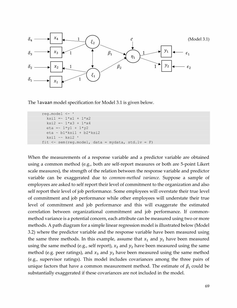
69

𝛿4 1 e (Model 3.1)

𝛿3 1 𝛽1 1 𝜖1

𝛿2 1 𝛽2 1 𝜖2

𝛿1 1

The lavaan model specification for Model 3.1 is given below.

reg.model <- '

ksi1 =~ 1*x1 + 1*x2

ksi2 =~ 1*x3 + 1*x4

eta =~ 1*y1 + 1*y2

eta ~ b1*ksi1 + b2*ksi2

ksi1 ~~ ksi2 '

fit <- sem(reg.model, data = mydata, std.lv = F)

When the measurements of a response variable and a predictor variable are obtained

using a common method (e.g., both are self-report measures or both are 5-point Likert

scale measures), the strength of the relation between the response variable and predictor

variable can be exaggerated due to common-method variance. Suppose a sample of

employees are asked to self report their level of commitment to the organization and also

self report their level of job performance. Some employees will overstate their true level

of commitment and job performance while other employees will understate their true

level of commitment and job performance and this will exaggerate the estimated

correlation between organizational commitment and job performance. If common-

method variance is a potential concern, each attribute can be measured using two or more

methods. A path diagram for a simple linear regression model is illustrated below (Model

3.2) where the predictor variable and the response variable have been measured using

the same three methods. In this example, assume that 𝑥1 and 𝑦1 have been measured

using the same method (e.g., self report), 𝑥2 and 𝑦2 have been measured using the same

method (e.g. peer ratings), and 𝑥3 and 𝑦3 have been measured using the same method

(e.g., supervisor ratings). This model includes covariances among the three pairs of

unique factors that have a common measurement method. The estimate of 𝛽1 could be

substantially exaggerated if these covariances are not included in the model.

𝑥4

𝑥3

𝑥2

𝑥1

𝜉2

𝜉1

𝜂1

𝑦1

𝑦2

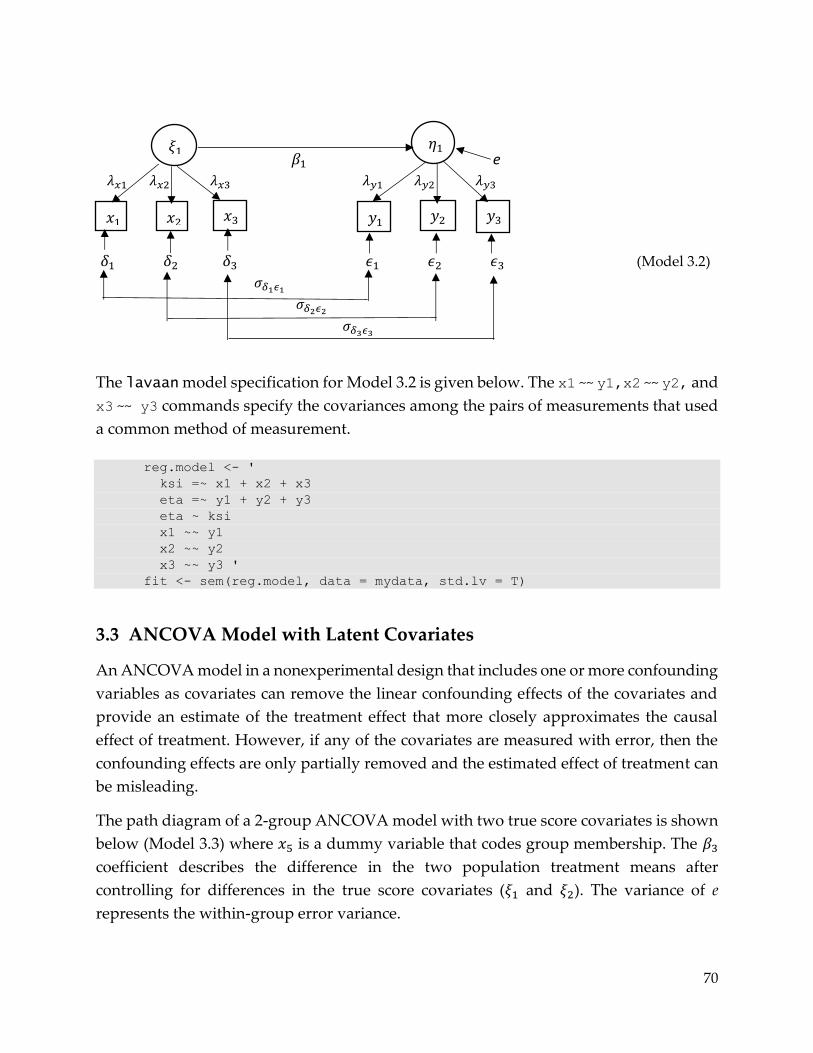
70

𝛽1 e 𝜆𝑥1 𝜆𝑥2 𝜆𝑥3 𝜆𝑦1 𝜆𝑦2 𝜆𝑦3

𝛿1 𝛿2 𝛿3 𝜖1 𝜖2 𝜖3 (Model 3.2)

𝜎𝛿1𝜖1

𝜎𝛿2𝜖2

𝜎𝛿3𝜖3

The lavaan model specification for Model 3.2 is given below. The x1 ~~ y1,x2 ~~ y2, and

x3 ~~ y3 commands specify the covariances among the pairs of measurements that used

a common method of measurement. reg.model <- '

ksi =~ x1 + x2 + x3

eta =~ y1 + y2 + y3

eta ~ ksi

x1 ~~ y1

x2 ~~ y2

x3 ~~ y3 '

fit <- sem(reg.model, data = mydata, std.lv = T)

3.3 ANCOVA Model with Latent Covariates

An ANCOVA model in a nonexperimental design that includes one or more confounding

variables as covariates can remove the linear confounding effects of the covariates and

provide an estimate of the treatment effect that more closely approximates the causal

effect of treatment. However, if any of the covariates are measured with error, then the

confounding effects are only partially removed and the estimated effect of treatment can

be misleading.

The path diagram of a 2-group ANCOVA model with two true score covariates is shown

below (Model 3.3) where 𝑥5 is a dummy variable that codes group membership. The 𝛽3

coefficient describes the difference in the two population treatment means after

controlling for differences in the true score covariates (𝜉1 and 𝜉2). The variance of e

represents the within-group error variance.

𝜉1

𝑥2 𝑥1

𝑥3

𝜂1

𝑦1 𝑦2

𝑦3

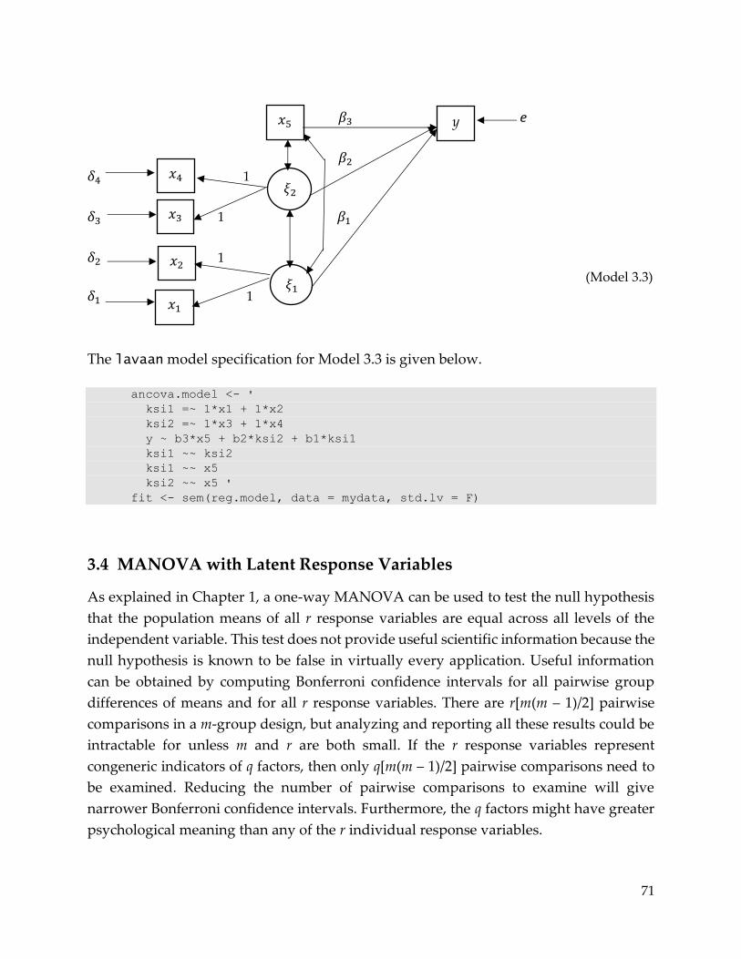
71

𝛽3 e

𝛽2 𝛿4 1

𝛿3 1 𝛽1

𝛿2 1

(Model 3.3)

𝛿1 1

The lavaan model specification for Model 3.3 is given below.

ancova.model <- '

ksi1 =~ 1*x1 + 1*x2

ksi2 =~ 1*x3 + 1*x4

y ~ b3*x5 + b2*ksi2 + b1*ksi1

ksi1 ~~ ksi2

ksi1 ~~ x5

ksi2 ~~ x5 '

fit <- sem(reg.model, data = mydata, std.lv = F)

3.4 MANOVA with Latent Response Variables

As explained in Chapter 1, a one-way MANOVA can be used to test the null hypothesis

that the population means of all r response variables are equal across all levels of the

independent variable. This test does not provide useful scientific information because the

null hypothesis is known to be false in virtually every application. Useful information

can be obtained by computing Bonferroni confidence intervals for all pairwise group

differences of means and for all r response variables. There are r[m(m – 1)/2] pairwise

comparisons in a m-group design, but analyzing and reporting all these results could be

intractable for unless m and r are both small. If the r response variables represent

congeneric indicators of q factors, then only q[m(m – 1)/2] pairwise comparisons need to

be examined. Reducing the number of pairwise comparisons to examine will give

narrower Bonferroni confidence intervals. Furthermore, the q factors might have greater

psychological meaning than any of the r individual response variables.

𝑥4

𝑥3

𝑥2

𝑥1

𝑥5 y

𝜉2

𝜉1

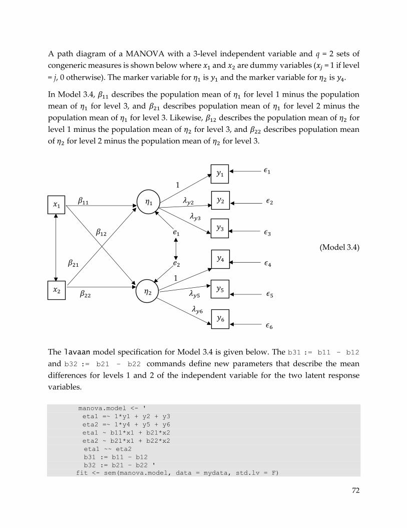
72

A path diagram of a MANOVA with a 3-level independent variable and q = 2 sets of

congeneric measures is shown below where 𝑥1 and 𝑥2 are dummy variables (𝑥𝑗 = 1 if level

= j, 0 otherwise). The marker variable for 𝜂1 is 𝑦1 and the marker variable for 𝜂2 is 𝑦4.

In Model 3.4, 𝛽11 describes the population mean of 𝜂1 for level 1 minus the population

mean of 𝜂1 for level 3, and 𝛽21 describes population mean of 𝜂1 for level 2 minus the

population mean of 𝜂1 for level 3. Likewise, 𝛽12 describes the population mean of 𝜂2 for

level 1 minus the population mean of 𝜂2 for level 3, and 𝛽22 describes population mean

of 𝜂2 for level 2 minus the population mean of 𝜂2 for level 3.

𝜖1

1

𝛽11 𝜆𝑦2 𝜖2

𝜆𝑦3

𝛽12 𝑒1 𝜖3

(Model 3.4)

𝛽21 𝑒2 𝜖4

1

𝛽22 𝜆𝑦5 𝜖5

𝜆𝑦6

𝜖6

The lavaan model specification for Model 3.4 is given below. The b31 := b11 – b12

and b32 := b21 – b22 commands define new parameters that describe the mean

differences for levels 1 and 2 of the independent variable for the two latent response

variables.

manova.model <- '

eta1 =~ 1*y1 + y2 + y3

eta2 =~ 1*y4 + y5 + y6

eta1 ~ b11*x1 + b21*x2

eta2 ~ b21*x1 + b22*x2

eta1 ~~ eta2

b31 := b11 – b12

b32 := b21 – b22 '

fit <- sem(manova.model, data = mydata, std.lv = F)

𝑦1

𝑥2

𝑥1 𝑦2

𝑦3

𝑦4

𝑦5

𝑦6

𝜂1

𝜂2

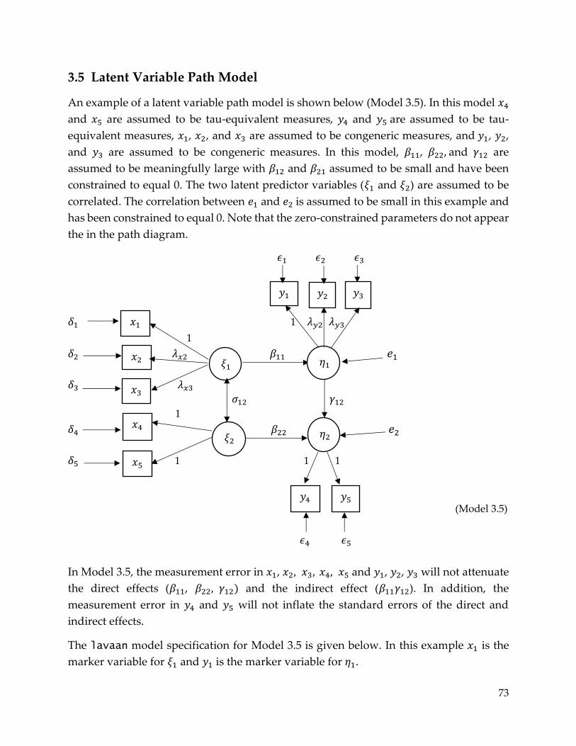
73

3.5 Latent Variable Path Model

An example of a latent variable path model is shown below (Model 3.5). In this model 𝑥4

and 𝑥5 are assumed to be tau-equivalent measures, 𝑦4 and 𝑦5 are assumed to be tau-

equivalent measures, 𝑥1, 𝑥2, and 𝑥3 are assumed to be congeneric measures, and 𝑦1, 𝑦2,

and 𝑦3 are assumed to be congeneric measures. In this model, 𝛽11, 𝛽22, and 𝛾12 are

assumed to be meaningfully large with 𝛽12 and 𝛽21 assumed to be small and have been

constrained to equal 0. The two latent predictor variables (𝜉1 and 𝜉2) are assumed to be

correlated. The correlation between 𝑒1 and 𝑒2 is assumed to be small in this example and

has been constrained to equal 0. Note that the zero-constrained parameters do not appear

the in the path diagram.

𝜖1 𝜖2 𝜖3

𝛿1 1 𝜆𝑦2 𝜆𝑦3

1

𝛿2 𝜆𝑥2 𝛽11 𝑒1

𝛿3 𝜆𝑥3 𝜎12 𝛾12

1

𝛿4 𝛽22 𝑒2

𝛿5 1 1 1

(Model 3.5)

𝜖4 𝜖5

In Model 3.5, the measurement error in 𝑥1, 𝑥2, 𝑥3, 𝑥4, 𝑥5 and 𝑦1, 𝑦2, 𝑦3 will not attenuate

the direct effects (𝛽11, 𝛽22, 𝛾12) and the indirect effect (𝛽11𝛾12). In addition, the

measurement error in 𝑦4 and 𝑦5 will not inflate the standard errors of the direct and

indirect effects.

The lavaan model specification for Model 3.5 is given below. In this example 𝑥1 is the

marker variable for 𝜉1 and 𝑦1 is the marker variable for 𝜂1.

𝑥2

𝑥3

𝑥4

𝑥5

𝑥1

𝑦1

𝜉1

𝜉2

𝜂2

𝜂1

𝑦2

𝑦3

𝑦5

𝑦4

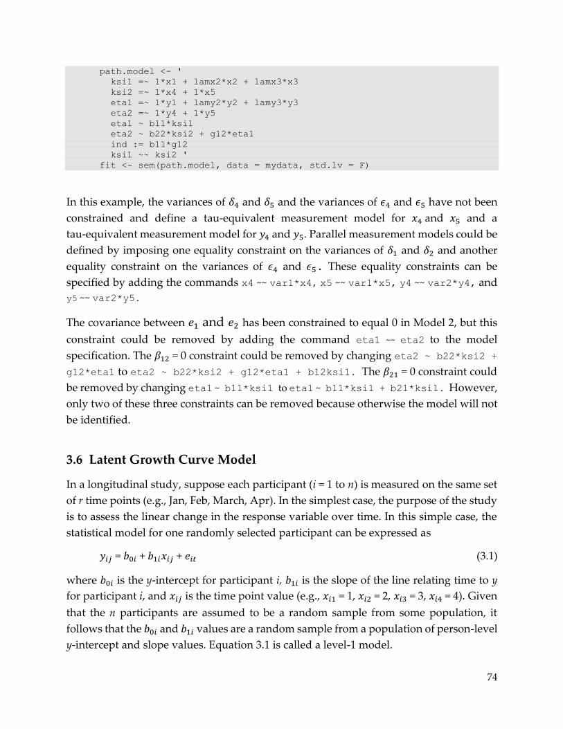
74

path.model <- '

ksi1 =~ 1*x1 + lamx2*x2 + lamx3*x3

ksi2 =~ 1*x4 + 1*x5

eta1 =~ 1*y1 + lamy2*y2 + lamy3*y3

eta2 =~ 1*y4 + 1*y5

eta1 ~ b11*ksi1

eta2 ~ b22*ksi2 + g12*eta1

ind := b11*g12

ksi1 ~~ ksi2 '

fit <- sem(path.model, data = mydata, std.lv = F)

In this example, the variances of 𝛿4 and 𝛿5 and the variances of 𝜖4 and 𝜖5 have not been

constrained and define a tau-equivalent measurement model for 𝑥4 and 𝑥5 and a

tau-equivalent measurement model for 𝑦4 and 𝑦5. Parallel measurement models could be

defined by imposing one equality constraint on the variances of 𝛿1 and 𝛿2 and another

equality constraint on the variances of 𝜖4 and 𝜖5. These equality constraints can be

specified by adding the commands x4 ~~ var1*x4, x5 ~~ var1*x5, y4 ~~ var2*y4, and

y5 ~~ var2*y5.

The covariance between 𝑒1 and 𝑒2 has been constrained to equal 0 in Model 2, but this

constraint could be removed by adding the command eta1 ~~ eta2 to the model

specification. The 𝛽12 = 0 constraint could be removed by changing eta2 ~ b22*ksi2 +

g12*eta1 to eta2 ~ b22*ksi2 + g12*eta1 + b12ksi1. The 𝛽21 = 0 constraint could

be removed by changing eta1 ~ b11*ksi1 to eta1 ~ b11*ksi1 + b21*ksi1. However,

only two of these three constraints can be removed because otherwise the model will not

be identified.

3.6 Latent Growth Curve Model

In a longitudinal study, suppose each participant (i = 1 to n) is measured on the same set

of r time points (e.g., Jan, Feb, March, Apr). In the simplest case, the purpose of the study

is to assess the linear change in the response variable over time. In this simple case, the

statistical model for one randomly selected participant can be expressed as

𝑦𝑖𝑗 = 𝑏0𝑖 + 𝑏1𝑖𝑥𝑖𝑗 + 𝑒𝑖𝑡 (3.1)

where 𝑏0𝑖 is the y-intercept for participant i, 𝑏1𝑖 is the slope of the line relating time to y

for participant i, and 𝑥𝑖𝑗 is the time point value (e.g., 𝑥𝑖1 = 1, 𝑥𝑖2 = 2, 𝑥𝑖3 = 3, 𝑥𝑖4 = 4). Given

that the n participants are assumed to be a random sample from some population, it

follows that the 𝑏0𝑖 and 𝑏1𝑖 values are a random sample from a population of person-level

y-intercept and slope values. Equation 3.1 is called a level-1 model.

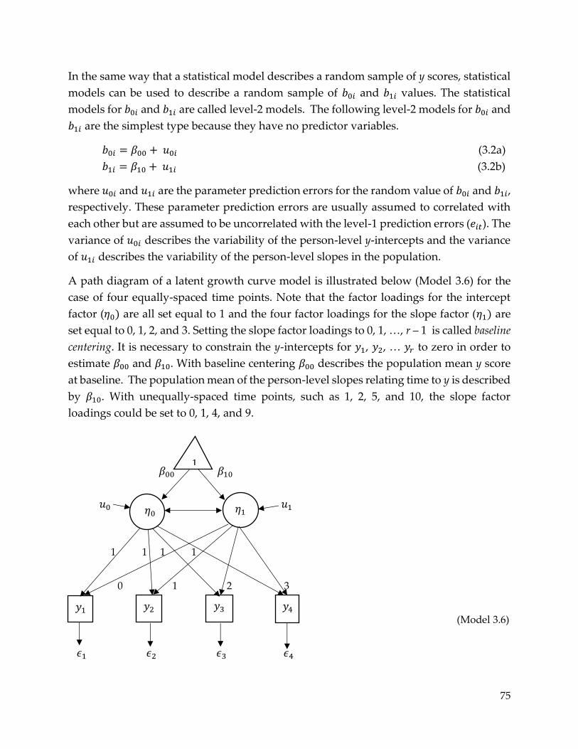
75

In the same way that a statistical model describes a random sample of y scores, statistical

models can be used to describe a random sample of 𝑏0𝑖 and 𝑏1𝑖 values. The statistical

models for 𝑏0𝑖 and 𝑏1𝑖 are called level-2 models. The following level-2 models for 𝑏0𝑖 and

𝑏1𝑖 are the simplest type because they have no predictor variables.

𝑏0𝑖 = 𝛽00 + 𝑢0𝑖 (3.2a)

𝑏1𝑖 = 𝛽10 + 𝑢1𝑖 (3.2b)

where 𝑢0𝑖 and 𝑢1𝑖 are the parameter prediction errors for the random value of 𝑏0𝑖 and 𝑏1𝑖,

respectively. These parameter prediction errors are usually assumed to correlated with

each other but are assumed to be uncorrelated with the level-1 prediction errors (𝑒𝑖𝑡). The

variance of 𝑢0𝑖 describes the variability of the person-level y-intercepts and the variance

of 𝑢1𝑖 describes the variability of the person-level slopes in the population.

A path diagram of a latent growth curve model is illustrated below (Model 3.6) for the

case of four equally-spaced time points. Note that the factor loadings for the intercept

factor (𝜂0) are all set equal to 1 and the four factor loadings for the slope factor (𝜂1) are

set equal to 0, 1, 2, and 3. Setting the slope factor loadings to 0, 1, …, r – 1 is called baseline

centering. It is necessary to constrain the y-intercepts for 𝑦1, 𝑦2, … 𝑦𝑟 to zero in order to

estimate 𝛽00 and 𝛽10. With baseline centering 𝛽00 describes the population mean y score

at baseline. The population mean of the person-level slopes relating time to y is described

by 𝛽10. With unequally-spaced time points, such as 1, 2, 5, and 10, the slope factor

loadings could be set to 0, 1, 4, and 9.

𝛽00 𝛽10

𝑢0 𝑢1

1 1 1 1

0 1 2 3

(Model 3.6)

𝜖1 𝜖2 𝜖3 𝜖4

𝑦1

𝜂0

𝜂1

𝑦2

𝑦3

𝑦4

1

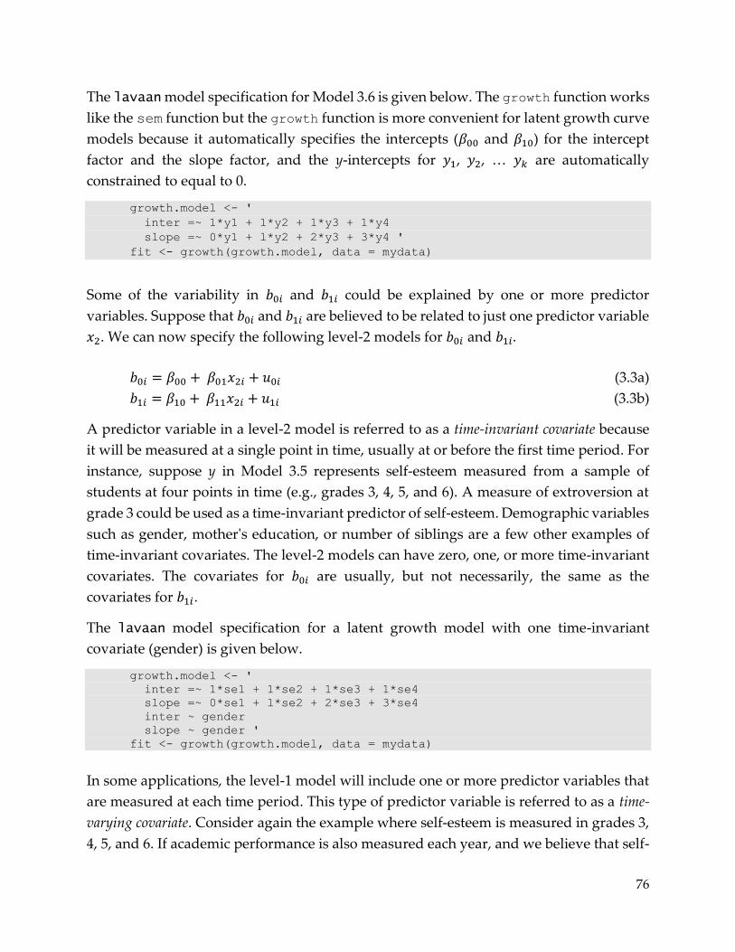
76

The lavaan model specification for Model 3.6 is given below. The growth function works

like the sem function but the growth function is more convenient for latent growth curve

models because it automatically specifies the intercepts (𝛽00 and 𝛽10) for the intercept

factor and the slope factor, and the y-intercepts for 𝑦1, 𝑦2, … 𝑦𝑘 are automatically

constrained to equal to 0.

growth.model <- '

inter =~ 1*y1 + 1*y2 + 1*y3 + 1*y4

slope =~ 0*y1 + l*y2 + 2*y3 + 3*y4 '

fit <- growth(growth.model, data = mydata)

Some of the variability in 𝑏0𝑖 and 𝑏1𝑖 could be explained by one or more predictor

variables. Suppose that 𝑏0𝑖 and 𝑏1𝑖 are believed to be related to just one predictor variable

𝑥2. We can now specify the following level-2 models for 𝑏0𝑖 and 𝑏1𝑖.

𝑏0𝑖 = 𝛽00 + 𝛽01𝑥2𝑖 + 𝑢0𝑖 (3.3a)

𝑏1𝑖 = 𝛽10 + 𝛽11𝑥2𝑖 + 𝑢1𝑖 (3.3b)

A predictor variable in a level-2 model is referred to as a time-invariant covariate because

it will be measured at a single point in time, usually at or before the first time period. For

instance, suppose y in Model 3.5 represents self-esteem measured from a sample of

students at four points in time (e.g., grades 3, 4, 5, and 6). A measure of extroversion at

grade 3 could be used as a time-invariant predictor of self-esteem. Demographic variables

such as gender, mother's education, or number of siblings are a few other examples of

time-invariant covariates. The level-2 models can have zero, one, or more time-invariant

covariates. The covariates for 𝑏0𝑖 are usually, but not necessarily, the same as the

covariates for 𝑏1𝑖.

The lavaan model specification for a latent growth model with one time-invariant

covariate (gender) is given below.

growth.model <- '

inter =~ 1*se1 + 1*se2 + 1*se3 + 1*se4

slope =~ 0*se1 + l*se2 + 2*se3 + 3*se4

inter ~ gender

slope ~ gender '


In some applications, the level-1 model will include one or more predictor variables that

are measured at each time period. This type of predictor variable is referred to as a time-

varying covariate. Consider again the example where self-esteem is measured in grades 3,

4, 5, and 6. If academic performance is also measured each year, and we believe that self-

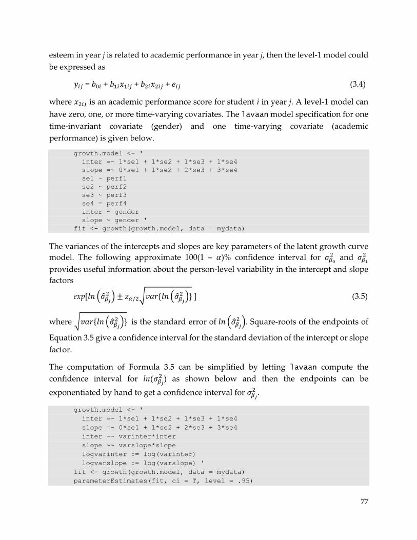
77

esteem in year j is related to academic performance in year j, then the level-1 model could

be expressed as

𝑦𝑖𝑗 = 𝑏0𝑖 + 𝑏1𝑖𝑥1𝑖𝑗 + 𝑏2𝑖𝑥2𝑖𝑗 + 𝑒𝑖𝑗 (3.4)

where 𝑥2𝑖𝑗 is an academic performance score for student i in year j. A level-1 model can

have zero, one, or more time-varying covariates. The lavaan model specification for one

time-invariant covariate (gender) and one time-varying covariate (academic

performance) is given below.

growth.model <- '

inter =~ 1*se1 + 1*se2 + 1*se3 + 1*se4

slope =~ 0*se1 + l*se2 + 2*se3 + 3*se4

se1 ~ perf1

se2 ~ perf2

se3 ~ perf3

se4 = perf4

inter ~ gender

slope ~ gender '


The variances of the intercepts and slopes are key parameters of the latent growth curve

model. The following approximate 100(1 – 𝛼)% confidence interval for 𝜎𝛽0

2 and 𝜎𝛽1

2

provides useful information about the person-level variability in the intercept and slope

factors

exp[𝑙𝑛 (�̂�𝛽𝑗

2 ) ± 𝑧𝛼/2√𝑣𝑎𝑟{𝑙𝑛 (�̂�𝛽𝑗

2 )} ] (3.5)

where √𝑣𝑎𝑟{𝑙𝑛 (�̂�𝛽𝑗

2 )} is the standard error of 𝑙𝑛 (�̂�𝛽𝑗

2 ). Square-roots of the endpoints of

Equation 3.5 give a confidence interval for the standard deviation of the intercept or slope

factor.

The computation of Formula 3.5 can be simplified by letting lavaan compute the

confidence interval for ln(𝜎𝛽𝑗

2 ) as shown below and then the endpoints can be

exponentiated by hand to get a confidence interval for 𝜎𝛽𝑗

2 .

growth.model <- '

inter =~ 1*se1 + 1*se2 + 1*se3 + 1*se4

slope =~ 0*se1 + l*se2 + 2*se3 + 3*se4

inter ~~ varinter*inter

slope ~~ varslope*slope

logvarinter := log(varinter)

logvarslope := log(varslope) '



78

The level-1 and level-2 models can be analyzed using “mixed linear model” statistical

programs. Unlike latent growth curve models, mixed linear model programs do not

require the same set of time periods for each participant. For example, mixed linear model

programs allow one participant to be measured on occasions 1, 2, 4, 6, a second

participant to be measured on occasions 3, 5, 9, and 10, a third participant to be measured

on occasions 1 and 7, and so on. The mixed linear model program in SPSS uses a

Satterthwaite degree of freedom adjustment which gives more accurate hypothesis tests

and confidence intervals than the approximate hypothesis tests and confidence intervals

obtained in a latent growth curve analysis.

However, if one or more of the predictor variables in the level-1 or level-2 models are

latent variables then the mixed model programs are of no use and a latent grown curve

model is required. Furthermore, a latent growth curve model can be part of a more

complex model where the intercept and slope factors are predictors of other observed or

latent variables and this type of analysis is not possible using mixed model programs.

The confidence intervals for 𝜎𝛽0

2 and 𝜎𝛽1

2 computed in mixed model programs assume the

person-level intercept and slope coefficients are normally distributed in the population,

and these confidence intervals can be very misleading when the normality assumption

has been violated. The normality assumption can be relaxed in a latent growth curve

analysis using optional robust standard errors or bootstrap standard errors.

3.7 Multiple-Group Latent Variable Models

Recall from Chapter 2 of Part 2 that an m-group design can be represented in a GLM by

including m – 1 dummy coded variables as predictor variables in the model along with

any quantitative predictor variables of y. Consider the most simple case of m = 2 groups

with one quantitative predictor of y that was described in section 2.16 of Part 2. Using

dummy coding, the following model includes one quantitative predictor variable (𝑥1),

one dummy coded variable (𝑥2) to code the two groups, and the product of 𝑥1 and 𝑥2 to

code the interaction between 𝑥1 and 𝑥2

𝑦𝑖 = 𝛽0 + 𝛽1𝑥1𝑖 + 𝛽2𝑥2𝑖 + 𝛽3(𝑥1𝑖𝑥2𝑖) + 𝑒𝑖. (3.6)

Alternatively, the above model can be represented by specifying two regression models,

one for each of the two groups as shown below

𝑦1𝑖 = 𝛽10 + 𝛽11𝑥11𝑖 + 𝑒1𝑖 (3.7a)

𝑦2𝑖 = 𝛽20 + 𝛽21𝑥21𝑖 + 𝑒2𝑖 (3.7b)

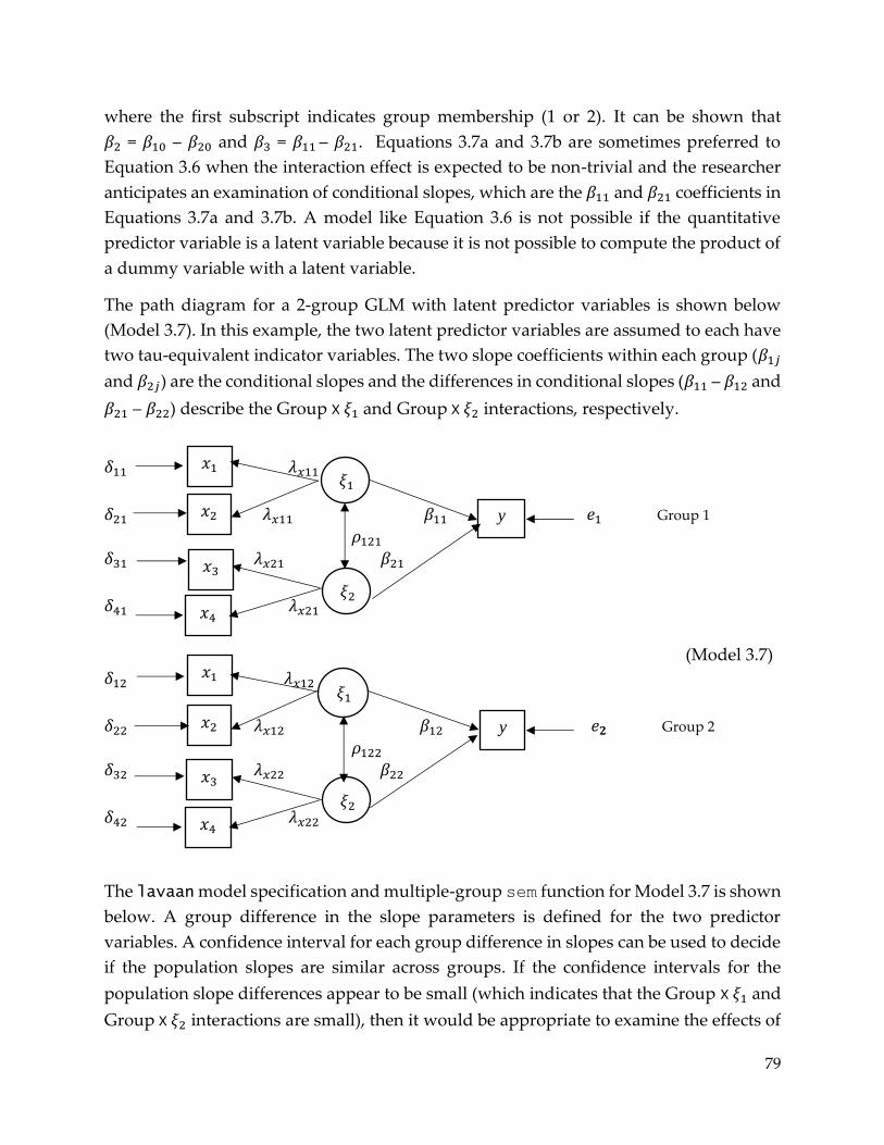
79

where the first subscript indicates group membership (1 or 2). It can be shown that

𝛽2 = 𝛽10 – 𝛽20 and 𝛽3 = 𝛽11 – 𝛽21. Equations 3.7a and 3.7b are sometimes preferred to

Equation 3.6 when the interaction effect is expected to be non-trivial and the researcher

anticipates an examination of conditional slopes, which are the 𝛽11 and 𝛽21 coefficients in

Equations 3.7a and 3.7b. A model like Equation 3.6 is not possible if the quantitative

predictor variable is a latent variable because it is not possible to compute the product of

a dummy variable with a latent variable.

The path diagram for a 2-group GLM with latent predictor variables is shown below

(Model 3.7). In this example, the two latent predictor variables are assumed to each have

two tau-equivalent indicator variables. The two slope coefficients within each group (𝛽1𝑗

and 𝛽2𝑗) are the conditional slopes and the differences in conditional slopes (𝛽11 – 𝛽12 and

𝛽21 – 𝛽22) describe the Group x 𝜉1 and Group x 𝜉2 interactions, respectively.

𝛿11 𝜆𝑥11

𝛿21 𝜆𝑥11 𝛽11 𝑒1 Group 1

𝜌121

𝛿31 𝜆𝑥21 𝛽21

𝛿41 𝜆𝑥21

(Model 3.7)

𝛿12 𝜆𝑥12

𝛿22 𝜆𝑥12 𝛽12 𝑒𝟐 Group 2

𝜌122 𝛿32 𝜆𝑥22 𝛽22

𝛿42 𝜆𝑥22

The lavaan model specification and multiple-group sem function for Model 3.7 is shown

below. A group difference in the slope parameters is defined for the two predictor

variables. A confidence interval for each group difference in slopes can be used to decide

if the population slopes are similar across groups. If the confidence intervals for the

population slope differences appear to be small (which indicates that the Group x 𝜉1 and

Group x 𝜉2 interactions are small), then it would be appropriate to examine the effects of

𝑥1

𝑥2

𝑥3

𝑥4

y

𝜉1

𝜉2

𝑥1

𝑥2

𝑥3

𝑥4

y

𝜉1

𝜉2

80

𝜉1 and 𝜉2 averaged over groups by adding the two commands b1ave := (b11 + b12)/2

and b2ave := (b21 + b22)/2.

twogroupGML.model <- '

ksi1 =~ c(lamx11,lamx12)*x1 + c(lamx11,lamx12)*x2

ksi2 =~ c(lamx21,lamx22)*x3 + c(lamx21,lamx22)*x4

y ~ c(b11,b12)*ksi1 + c(b21,b22)*ksi2

b1diff := b11 – b12

b2diff := b21 – b22 '

fit <- sem(twogroupGLM.model, data = mydata, std.lv = T, group = "group")

3.8 Model Assessment

All theoretically important model parameters should be meaningfully large and all zero-

constrained parameters should be small. As a general recommendation for parameters

that have been included in the model, the population standardized slope coefficients

should be greater than .2 in absolute value (larger is better) and population standardized

factor loadings should be greater than .3 in absolute value (larger is better). Theoretically

important population correlations among factors or observed variables should also be

greater than .2 in absolute value. Confidence intervals for population standardized

slopes, population standardized factor loadings, and population correlations can be used

to assess the magnitude of these parameters. Specifically, a 95% confidence interval

should be completely outside the -.2 to .2 range for a standardized slope or correlation

and completely outside the -.3 to .3 range for a standardized factor loading. Ideally, 95%

Bonferroni confidence intervals for the included parameters will indicate that all included

parameters are meaningfully large.

Modification indices are useful in assessing latent variable model misspecification.

Modification indices for factor loadings should be examined first. The zero-constrained

factor loading with the largest modification index can be added to the model, and if the

95% confidence interval for the added factor loading is completely contained within the

-.3 to .3 range (smaller is better), then the researcher could argue that constraining this

loading to zero is justifiable. If the 95% confidence interval for the standardized factor

loading with the largest modification index when added to the model is completely

contained within the -.3 to .3 range, it is likely that all other factors loadings that were

zero-constrained are also small. If the 95% confidence interval for the added loading is

completely outside the -.3 to .3 range, then this loading should be retained in the model

(assuming this loading can be theoretically justified) and all model parameters need to

be re-estimated. The factor loading with the largest modification index in the revised

81

model should then be assessed. If the confidence interval for the added standardized

factor loading includes -.3 or .3, the statistical results are “inconclusive” and the

researcher must decide to include or exclude that factor loading based on non-statistical

criteria. Ideally the confidence interval for assessing an added factor loading should use

an adjusted alpha level of 𝛼/𝑘 where k is the number of zero-constrained factor loadings.

After the zero-constrained factor loadings have been assessed, the zero-constrained

slopes should examined. The path for the slope with the largest modification index

should be added to the model. If the 95% confidence interval for the standardized slope

of the added path is completely contained within the -.2 to .2 range, then the researcher

could argue that constraining this slope to zero is justifiable and it is likely that all other

zero-constrained slopes also are small. If the 95% confidence interval for the standardized

slope of the added path is completely outside the -.2 to .2 range, then this path should be

included in the model (assuming this path can be theoretically justified) and all the

parameters of the model need to be re-estimated. The zero-constrained slope with the

largest modification index in the revised model should then be examined. If the

confidence interval for the standardized slope of the added path includes -.2 or .2, the

statistical results are “inconclusive” and the researcher must decide to include or exclude

that path based on non-statistical criteria. Ideally the confidence interval for assessing an

added path should use an adjusted alpha level of 𝛼/𝑘 where k is the number of zero-

constrained slopes.

In a multiple-group design, equivalence tests should be used to assess parameter

similarity across groups. Equivalence tests require the researcher to specify a range of

practical equivalence which is usually easier to do for standardized rather than

unstandardized slopes and factor loadings. Although a narrow range of practical

equivalence will provide more compelling evidence of similarity, a narrow range also

requires a very large sample size.

If several constrained parameters are unconstrained after an exploratory examination of

the modification indices, the p-values and confidence intervals in the final model can be

misleading. At a minimum, all exploratory modifications should be described in the

research report. Ideally, the final model will be reanalyzed in a new random sample. If

the researcher has access to a very large random sample, the sample can be randomly

divided into two samples with the exploratory analysis performed in the first sample (the

"training" sample) and a confirmatory analysis performed in the second sample (the "test"

sample). Only the results in the test sample should be reported.

82

Chi-square GOF tests are commonly used to assess the path models in Chapter 1 and all

of the models in Chapters 2 and 3. The GOF test is a test of the null hypothesis that all

constraints on the model are correct (i.e., all zero-constrained parameters equal 0 and all

equality constrained parameters are equal). The GOF test is routinely misinterpreted.

Researchers incorrectly interpret a p-value greater than .05 as evidence that the model is

“correct”. In fact, the null hypothesis is almost never correct in any real application and

the p-value can exceed .05 in small samples even if the model is badly misspecified. In

large samples, the p-value for a GOF test can be much less than .05 in models that are

only trivially misspecified. However, a small p-value for the GOF tests could indicate

non-trivial model misspecification if the sample size is small (n < 200).

Chi-square model comparison tests are also very popular. In multiple-group designs, one

model might allow corresponding parameter values to differ across groups and another

model constrains these parameters to be equal across groups. The chi-squared model

comparison test in this example is a test of the null hypothesis that all corresponding

parameters are equal across groups. This test is routinely misinterpreted. Researchers will

interpret a p-value greater than .05 as evidence that all corresponding parameters are

equal across groups, and a p-value less than .05 is reported as a “significant difference”

across groups. In fact, a p-value less than .05 does not imply the parameters are equal,

and a p-value greater than .05 does not imply that the parameter values are meaningfully

different. Equivalence tests are needed to determine if the corresponding parameter

values are similar or dissimilar across groups. Of course, equivalence tests usually require

very large sample sizes.

Model comparison tests are also used to compare a model that includes all of the

theoretically specified path parameters with a second model that omits all of these

parameters. If the p-value for the chi-square model comparison test is less than .05,

researchers incorrectly interpret this result as evidence that the model with the omitted

paths is “incorrect” or “unacceptable”. Despite the serious limitations of the GOF and

model comparison tests, most psychology journals expect authors to report the results of

a GOF test and possibly the results of a model comparison test along with one or more fit

indices such as CFI and RMSEA. The recommendation here is to supplement the reported

fit indices, chi-squared values, and p-values with confidence intervals for all theoretically

important parameters in the final model. It is also important to report the confidence

intervals for the largest zero-constrained factor loading and the largest zero-constrained

slope after removing the constraints to show that the constraints are justified. If the results

for a zero-constrained slope are inconclusive and the slope corresponds to a path that, if

included in the model, would fundamentally change the conclusions of the study, it is

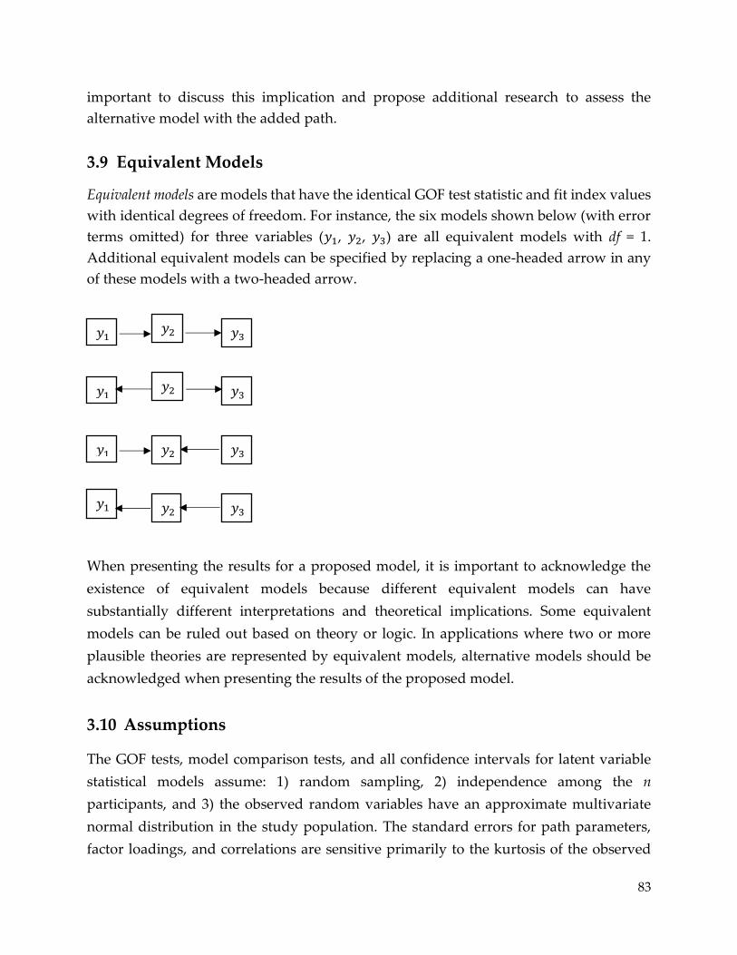
83

important to discuss this implication and propose additional research to assess the

alternative model with the added path.

3.9 Equivalent Models

Equivalent models are models that have the identical GOF test statistic and fit index values

with identical degrees of freedom. For instance, the six models shown below (with error

terms omitted) for three variables (𝑦1, 𝑦2, 𝑦3) are all equivalent models with df = 1.

Additional equivalent models can be specified by replacing a one-headed arrow in any

of these models with a two-headed arrow.

When presenting the results for a proposed model, it is important to acknowledge the

existence of equivalent models because different equivalent models can have

substantially different interpretations and theoretical implications. Some equivalent

models can be ruled out based on theory or logic. In applications where two or more

plausible theories are represented by equivalent models, alternative models should be

acknowledged when presenting the results of the proposed model.

3.10 Assumptions

The GOF tests, model comparison tests, and all confidence intervals for latent variable

statistical models assume: 1) random sampling, 2) independence among the n

participants, and 3) the observed random variables have an approximate multivariate

normal distribution in the study population. The standard errors for path parameters,

factor loadings, and correlations are sensitive primarily to the kurtosis of the observed

𝑦2

𝑦1

𝑦3

𝑦2

𝑦1

𝑦3

𝑦2

𝑦1

𝑦3

𝑦2

𝑦1

𝑦3

84

variables. The standard errors will be too small with leptokurtic distributions and too

large with platykurtic distributions regardless of sample size. Since confidence interval

results provide the best way to assess a model, leptokurtosis is more serious than

platykurtosis because the confidence intervals will be misleadingly narrow with

leptokurtic distributions. As noted in Chapter 2, if the normality assumption for any

particular observed variable has been violated, it might be possible to reduce skewness

and kurtosis by transforming that variable. Data transformations might also help reduce

nonlinearity and heteroscedasticity. If remedial measures cannot remove excess kurtosis,

confidence intervals should be computed using robust or bootstrap standard errors.

In latent variable statistical models, which are usually more complex than the models in

Chapters 1 and 2, the recommendation here is to use a sample size of at least 200 when

using ML estimation with robust or bootstrap standard errors. With multiple-group

models, a sample size of at least 100 per group is recommended. For indirect effects,

which can have highly nonnormal sampling distributions, Monte Carlo confidence

intervals are recommended. For GOF tests and fit indices, the mean adjusted (Satorra-

Bentler) test statistic based on ML estimates is recommended.

3.11 Sample Size Recommendations

There are two completely separate issues regarding sample size requirements for the tests

and confidence intervals presented in Chapters 1, 2, and 3. One issue is the sample size

required for a test or confidence interval to perform properly. A 95% confidence interval

for some parameter is said to perform properly in a sample of size n if about 95% of the

confidence intervals computed from all possible samples of size n would contain the

parameter value. A directional hypothesis test with 𝛼 = .05 in a sample of size n is said

to perform properly if a directional error is made in at most 2.5% of all possible samples

of size n. All of the tests and confidence intervals for unstandardized slopes in the GLM,

MGLM, and recursive path models will perform properly in small samples if their

assumptions (e.g., random sampling, independence among participants, linearity, equal

prediction error variance, prediction error normality) have been satisfied. If the observed

variables in a latent variable statistical model are platykurtic or at most moderately

leptokurtic, confidence intervals and hypothesis tests based on ML estimates with robust

or bootstrap standard errors should perform properly with sample sizes of at least 200.

Some research suggests that confidence intervals based on ULS estimates with robust

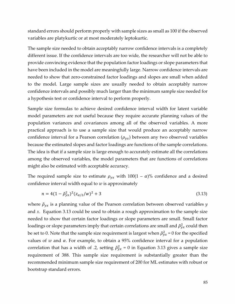
85

standard errors should perform properly with sample sizes as small as 100 if the observed

variables are platykurtic or at most moderately leptokurtic.

The sample size needed to obtain acceptably narrow confidence intervals is a completely

different issue. If the confidence intervals are too wide, the researcher will not be able to

provide convincing evidence that the population factor loadings or slope parameters that

have been included in the model are meaningfully large. Narrow confidence intervals are

needed to show that zero-constrained factor loadings and slopes are small when added

to the model. Large sample sizes are usually needed to obtain acceptably narrow

confidence intervals and possibly much larger than the minimum sample size needed for

a hypothesis test or confidence interval to perform properly.

Sample size formulas to achieve desired confidence interval width for latent variable

model parameters are not useful because they require accurate planning values of the

population variances and covariances among all of the observed variables. A more

practical approach is to use a sample size that would produce an acceptably narrow

confidence interval for a Pearson correlation (𝜌𝑦𝑥) between any two observed variables

because the estimated slopes and factor loadings are functions of the sample correlations.

The idea is that if a sample size is large enough to accurately estimate all the correlations

among the observed variables, the model parameters that are functions of correlations

might also be estimated with acceptable accuracy.

The required sample size to estimate 𝜌𝑦𝑥 with 100(1 – 𝛼)% confidence and a desired

confidence interval width equal to w is approximately

𝑛 = 4(1 − �̃�𝑦𝑥2 )2(𝑧𝛼/2/𝑤)2 + 3 (3.13)

where �̃�𝑦𝑥 is a planning value of the Pearson correlation between observed variables y

and x. Equation 3.13 could be used to obtain a rough approximation to the sample size

needed to show that certain factor loadings or slope parameters are small. Small factor

loadings or slope parameters imply that certain correlations are small and �̃�𝑦𝑥2 could then

be set to 0. Note that the sample size requirement is largest when �̃�𝑦𝑥2 = 0 for the specified

values of w and 𝛼. For example, to obtain a 95% confidence interval for a population

correlation that has a width of .2, setting �̃�𝑦𝑥2 = 0 in Equation 3.13 gives a sample size

requirement of 388. This sample size requirement is substantially greater than the

recommended minimum sample size requirement of 200 for ML estimates with robust or

bootstrap standard errors.

86

If the sample can be obtained in two stages, it is possible to approximate the number of

participants in the second-stage sample that should be added to the first-stage sample.

Suppose the size of the first-stage sample is 𝑛1 and 𝑤1 is the width of a confidence interval

for the most important effect in the model. An effect might be the RMSEA, a single slope

or factor loading, or a difference in slopes or factor loadings. To achieve the desired

confidence interval width (w) of a confidence interval for the specified effect, the number

of participants to sample in the second stage is approximately

𝑛2 = 𝑛1[(𝑤1/𝑤)2 − 1]. (3.14)

The first-stage and second-stage samples should be taken from the same study

population and the second-stage sample is combined with the first-stage sample. The

parameters of the latent variable model are then estimated from the combined sample of

size 𝑛1 + 𝑛2.

87

Key Terms

latent variable path model

common method variance

latent growth curve model

level-1 model

level-2 model

baseline centering

time-invariant covariate

time-varying covariate

multiple-group model

measurement invariance

equivalent models

Concept Questions

1. What is the benefit of using a latent predictor variable?

2. What is the benefit of using a latent response variable?

3. What is the effect of measurement error on indirect effects?

4. Why is baseline centering often used in latent growth curve models?

5. Explain how goodness of fit tests are misused.

6. What is the effect of kurtosis on the GOF test statistic and standard errors?

7. How could you show that the included paths in a latent variable path model are

meaningfully large.

8. How could you show that the omitted paths in a latent variable path model are small

or unimportant?

9. When would you consider using a bootstrap confidence intervals?

10. How can interaction effects be estimated in a multiple group model?

88

11. When would you use a latent variable growth curve model in lavaan rather than a

mixed model program in SPSS or SAS?

12. What is the advantage of using an ANCOVA model with latent covariates over the

traditional ANCOVA?

13. Why is it important to discuss equivalent models when reporting the results of a

particular model?

14. Give the lavaan model specification code for a MGLM with two latent predictor

variables, two latent responses variables, with all latent variables having two indicators.

15. Give the lavaan model specification code for a path model where two latent predictor

variables predict one latent mediator variable which predicts an observed response

variable. The two latent predictor variables each have three indicators and the latent

mediator variable has two indicators.

16. Give the lavaan model specification code for a latent growth curve model with three

time periods where 𝜉1 predicts the latent intercept and the latent slope, and 𝑥1 and 𝑥2 are

tau-equivalent indicators of 𝜉1.

89


3-1. Three parallel measures of a practice FCC commercial radio license exam were

developed to help prospective examinees study for actual exam. Jobs that require a

commercial radio license tend to be male dominated, and the FCC wants to verify that

the practice exams do not exhibit any substantial gender differences in terms of the factor

loadings or measurement error variability. A random sample of 175 men and 100 women,

taken from a study population of about 2,500 men and 600 women who paid for study

guide materials, were told they would receive the materials for free if they simply agreed

to anonymously take the three practice tests. The 214BHW3-1.sav file contains the

sample data for the 275 men and women. The variable names are FormA, FormB, FormC,

and sex (sex = 1 for men and sex = 2 for women).

a) Compute 95% confidence intervals for the standardized factor loading in each group

and report the results.

b) Compute a 95% confidence interval for the gender difference in standardized factor

loadings and report the result.

c) Compute a 95% confidence interval for the ratio of error standard deviations for men

and women and report the result.

d) Compute a 95% confidence interval for the average standardized factor loadings for

men and women and report the results.

e) Report the GOF test statistic, df, p-value, CFI, and RMSEA values.

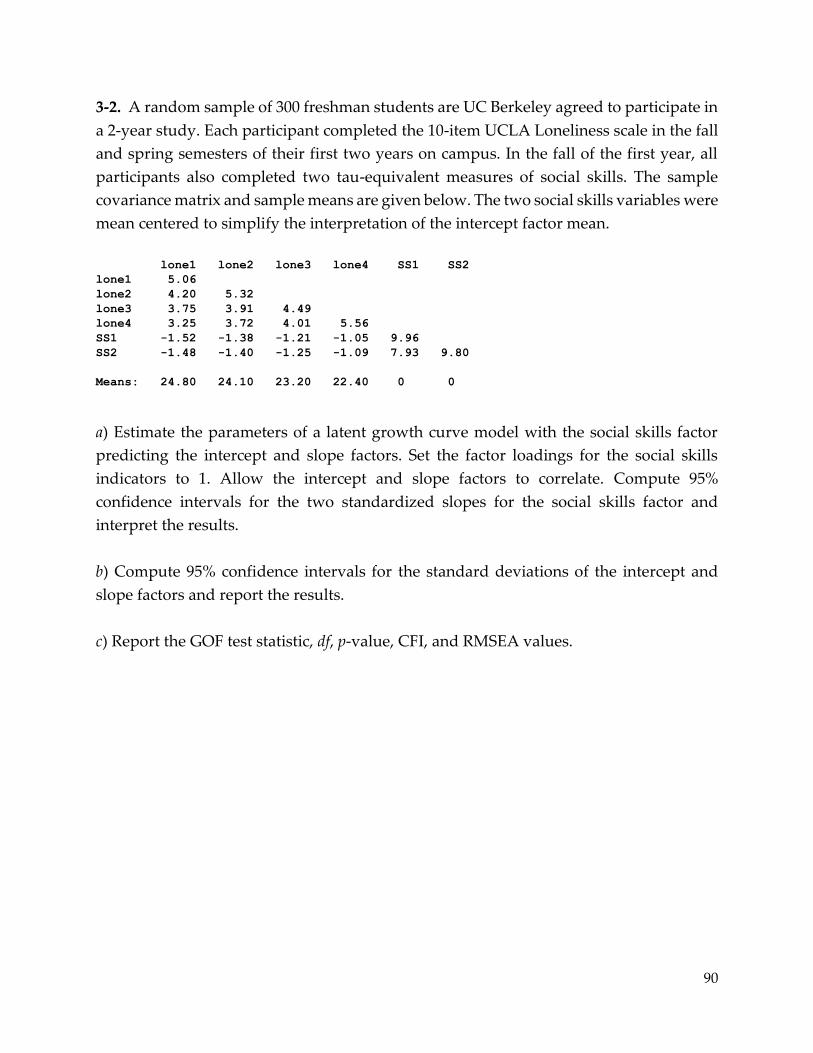
90

3-2. A random sample of 300 freshman students are UC Berkeley agreed to participate in

a 2-year study. Each participant completed the 10-item UCLA Loneliness scale in the fall

and spring semesters of their first two years on campus. In the fall of the first year, all

participants also completed two tau-equivalent measures of social skills. The sample

covariance matrix and sample means are given below. The two social skills variables were

mean centered to simplify the interpretation of the intercept factor mean.

lone1 lone2 lone3 lone4 SS1 SS2

lone1 5.06

lone2 4.20 5.32

lone3 3.75 3.91 4.49

lone4 3.25 3.72 4.01 5.56

SS1 -1.52 -1.38 -1.21 -1.05 9.96

SS2 -1.48 -1.40 -1.25 -1.09 7.93 9.80

Means: 24.80 24.10 23.20 22.40 0 0

a) Estimate the parameters of a latent growth curve model with the social skills factor

predicting the intercept and slope factors. Set the factor loadings for the social skills

indicators to 1. Allow the intercept and slope factors to correlate. Compute 95%

confidence intervals for the two standardized slopes for the social skills factor and

interpret the results.

b) Compute 95% confidence intervals for the standard deviations of the intercept and

slope factors and report the results.

c) Report the GOF test statistic, df, p-value, CFI, and RMSEA values.

91

3-3. A study of workplace micro-aggression was conducted at a large high-tech

organization of about 200,000 employees. A random sample of 300 employees was

obtained from the company’s human resource database. The job grade (on a 1 to 25 scale)

was recorded for each participant, and each participant completed a micro-aggression 20-

item checklist (scored on a 20 to 80 scale). The researchers believe that employees with

lower job grades are targets of more micro-aggressive acts than employees with higher

pay grades, and they suspect that an employee’s level of social dominance might mediate

this relation. Each participant completed three different social dominance questionnaires.

The 214BHW3-3.sav file contains the sample data with variable names grade,

socdom1, socdom2, socdom3, and microaggr.

a) Estimate the parameters of a latent variable path model using ULS estimation with

robust standard errors in which grade predicts a social dominance factor defined by

three congeneric indicators (socdom1, socdom2, socdom3), and the social dominance

factor predicts microaggr. Compute 95% confidence intervals for the two standardized

slope parameters and report the results.

b) Estimate the standardized indirect effect of grade on microaggr and compute a 95%

confidence interval for this effect. Report the results.

c) Report the Satorra-Bentler GOF chi-square (using ML estimates), df, and p-value. Also

report the CFI and RMSEA values (using ML estimates).

d) Include a path from grade to microaggr in the model. Compute a 95% confidence

interval for this standardized slope parameter using ULS estimation with robust standard

errors and explain why this path can be assumed to be small and omitted from the model.

92

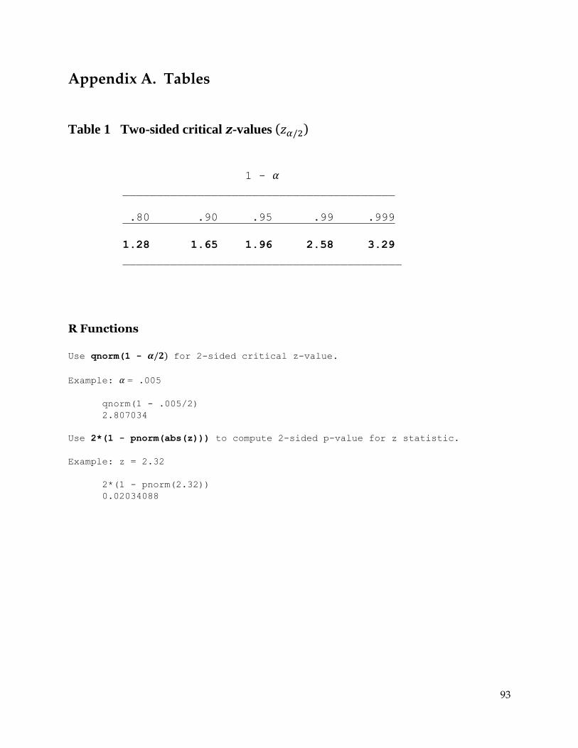
93

Appendix A. Tables

Table 1 Two-sided critical z-values (𝑧𝛼/2)

1 - 𝛼 ________________________________________

.80 .90 .95 .99 .999

1.28 1.65 1.96 2.58 3.29

_________________________________________

R Functions

Use qnorm(1 - 𝜶/𝟐) for 2-sided critical z-value.

Example: 𝛼 = .005

qnorm(1 - .005/2)

2.807034

Use 2*(1 - pnorm(abs(z))) to compute 2-sided p-value for z statistic.

Example: z = 2.32

2*(1 - pnorm(2.32))

0.02034088

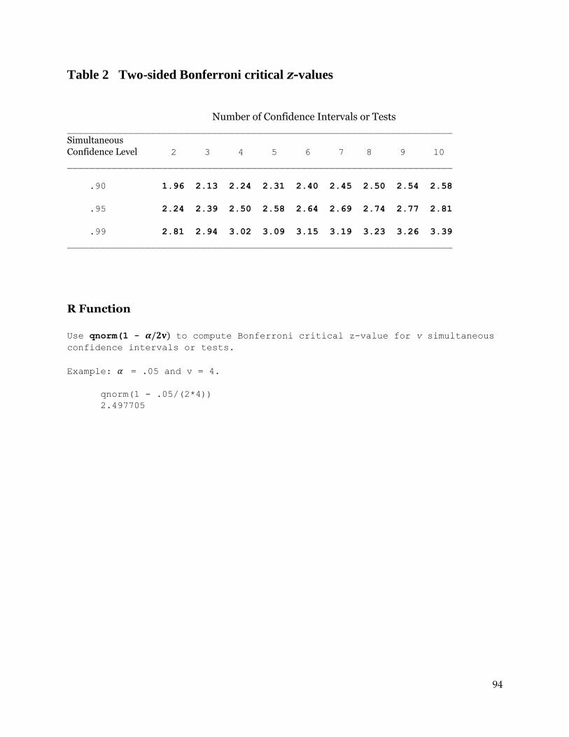
94

Table 2 Two-sided Bonferroni critical z-values

Number of Confidence Intervals or Tests _____________________________________________________________________

Simultaneous

Confidence Level 2 3 4 5 6 7 8 9 10

_____________________________________________________________________

.90 1.96 2.13 2.24 2.31 2.40 2.45 2.50 2.54 2.58

.95 2.24 2.39 2.50 2.58 2.64 2.69 2.74 2.77 2.81

.99 2.81 2.94 3.02 3.09 3.15 3.19 3.23 3.26 3.39

_____________________________________________________________________

R Function

Use qnorm(1 - 𝜶/𝟐𝐯) to compute Bonferroni critical z-value for v simultaneous

confidence intervals or tests.

Example: 𝛼 = .05 and v = 4.

qnorm(1 - .05/(2*4))

2.497705

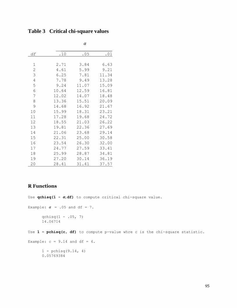
95

Table 3 Critical chi-square values

𝛼 ____________________

df .10 .05 .01

1 2.71 3.84 6.63

2 4.61 5.99 9.21

3 6.25 7.81 11.34

4 7.78 9.49 13.28

5 9.24 11.07 15.09

6 10.64 12.59 16.81

7 12.02 14.07 18.48

8 13.36 15.51 20.09

9 14.68 16.92 21.67

10 15.99 18.31 23.21

11 17.28 19.68 24.72

12 18.55 21.03 26.22

13 19.81 22.36 27.69

14 21.06 23.68 29.14

15 22.31 25.00 30.58

16 23.54 26.30 32.00

17 24.77 27.59 33.41

18 25.99 28.87 34.81

19 27.20 30.14 36.19

20 28.41 31.41 37.57

R Functions

Use qchisq(1 - 𝜶, df) to compute critical chi-square value.

Example: 𝛼 = .05 and df = 7.

qchisq(1 - .05, 7)

14.06714

Use 1 – pchisq(c, df) to compute p-value whre c is the chi-square statistic.

Example: c = 9.14 and df = 4.

1 - pchisq(9.14, 4)

0.05769384

96

97

Appendix B. Glossary

alternate form reliability – a measure of reliability defined from two or more measurements

of some attribute obtained from two or more equivalent forms of a test

baseline centering – coding of time points with time 1 set to 0

bootstrap standard errors – a computationally intensive method to obtain approximate

distribution-free standard errors

CFI – (comparative fit index) a measure of model misspecification that has a range from

0 to 1 with values closer to 1 indicating less misspecification

chi-squared goodness of fit test – a test of the null hypothesis that all of the constrained

parameters in a model are equal to their constrained values with degrees of freedom

equal to the number of constraints

chi-squared model comparison test – a difference in chi-square test statistic values for a full

model and a reduced model where the reduced model is nested in the full model and the

degrees of freedom are equal to the difference in degrees of freedom for the two chi-

square tests

common method variance – the introduction of bias into a correlation or slope as a result of

measuring the variables using a common method of measurement

communality – the proportion of the variance of a given indicator variable that is

predictable from all of the factors

conditional direct effect – the effect (described by a slope) of a predictor variable on a

response variable at one level of a moderator variable

conditional indirect effect – an indirect effect (described by a product of slopes) in a path

model at one level of a moderator variable

confirmatory factor analysis model – a factor analysis model with enough parameter

constraints to allow unique estimation of unconstrained model parameters; the number

of factors and the unconstrained factor loadings are presumably determined prior to data

collection

confounding variable – a variable that is correlated with the dependent variable and some

predictor variable

congeneric measurement model – a 1-factor factor analysis model

Cronbach’s alpha coefficient – a measure of reliability of the sum or average of two or more

tau-equivalent measurements

98

direct effect – the effect (described by a slope) of a predictor variable on a response variable

direct oblimin method – an oblique rotation method in an exploratory factor analysis

endogenous variable – any variable in a path model that is predicted by some other variable

equivalent models – two models with the same set of variables, fit index values, GOF test

values, and degrees of freedom but with paths having different directions

exogenous variable – predictor variable in a path model that is not predicted by any other

variable

exploratory factor analysis – a factor analysis in which all factor loadings and factor

correlations are estimated but these loadings and correlations are not unique; the number

of factors is often determined in an exploratory manner

factor loading – a regression coefficient in a measurement model where the response

variable is an observed variable and the predictor variable is a latent variable

general linear model – a linear statistical model for a quantitative response variable where

the predictor variables can be indicator variables, quantitative variables, or any

combination of indicator and quantitative predictors

GOF test – a test of the null hypothesis that all of the constrained parameters in a model

are equal to the constrained values

goodness of fit function – a function that is minimized in the computation of parameter

estimates

indirect effect – the effect of one variable (described by a product of slopes) on another

variable that is mediated by another variable

internal consistency reliability – a measure of reliability defined from responses to multiple

items of a questionnaire

inter-rater reliability – a measure of reliability defined from the ratings of multiple raters

latent growth curve model – a latent variable model where the random y-intercept and

random slopes are represented by latent variables

latent variable path model – a path model where one or more variables are latent variables

level-1 model – in a multi-level model for repeated measurements, the level-1 model

describes the relation between the response variable and the time-varying covariates

level-2 model – in a multi-level model for repeated measurements, the level-2 model

describes the relation between the random coefficients in the level-1 model and the time-

invariant covariates

99

listwise deletion – removing a participant if that participant has missing data on any

variable that is used in a statistical model

MANOVA model – a special case of the multivariate general linear model where all the

predictor variables are indicator variables

MANCOVA model – a special case of the general linear model where some predictor

variables are indicator variables and other predictor variables are quantitative variables

McDonald’s omega coefficient – a measure of the reliability of a sum or average of two or

more congeneric measurements

marker variable – the variable in a measure model or CFA model that has its factor loading

constrained equal to 1to identify the model

measurement error – the difference between an object's true score for some attribute and

that object's measured score for that attribute

measurement invariance – equality of factor loadings and unique factor variances across

two or more groups

mediator variable – a variable that is assumed to be caused by one or more predictor

variables and also has a causal effect on one or more response variables

missing at random – missingness for a given variable that is unrelated to that variable and

all variables not included in the model

missing completely at random – missingness for a given variable that is unrelated to that

variable and all variables included in the model and all variables not included in the

model

ML estimation – (maximum likelihood estimation) a method of parameter estimation that

maximizes the likelihood function under an assumption of multivariate normality and

produces estimates with the smallest possible standard errors (assuming multivariate

normality)

modification index – a test statistic for any constrained parameter that tests the null

hypothesis that the constraint is correct

multiple-group model – a structural equation model where a model is defined within each

of two or more groups

multivariate general linear model – a linear statistical model for two or more quantitative

response variables where the predictor variables can be indicator variables, quantitative

variables, or any combination of indicator and quantitative predictors

100

NFI – (normed fit index) a measure of model misspecification that has a range from 0 to

1 with values closer to 1 indicating less misspecification; the NFI is negatively biased in

small samples

nonrecursive model – a path model with correlated prediction errors or feedback paths

oblique rotation – a method of transforming the factor loadings to improve interpretability

and allowing the factors to be correlated

orthogonal rotation – a method of transforming the factor loadings in an exploratory factor

analysis to improve interpretability with the constraint that the factors are uncorrelated

parallel measurement model – a 1-factor factor analysis model where all factor loadings are

equal and all unique factor variances are equal

path model – a linear statistical model for two or more response variables where one or

more response variable can predictor another response variable

pattern matrix – a matrix of standardized or unstandardized factor loadings for all factors

and all indicator variables

promax method – an oblique rotation method in an exploratory factor analysis

recursive model – a path model with no correlated prediction errors and no feedback paths

RMSEA – (root mean square error of approximation) a measure of model misspecification

that has a range from 0 to 1 with values closer to 0 indicating less misspecification

robust standard errors – approximate standard errors that do not assume multivariate

normality

Satorra-Bentler scaled chi-square – a goodness of fit test statistic that does not assume

multivariate normality

scree plot – an ordered plot of the eigenvalues associated with each factor that can be used

to approximate the required number of factors in an exploratory factor analysis

semipartial correlation – the correlation between the component of a predictor variable that

is not linearly related to the other predictor variables with the response variable;

describes the standard deviation change in the response variable associated with a one

standard deviation change in the component of a predictor variable that is not linearly

related to the other predictor variables

Spearman-Brown formula – a formula that can be used to convert the reliability of an

average of multiple measurements to the reliability of a single measurement

101

standardized factor loading – a factor loading where the variance of the factor and the

variance of the indicator is set to 1

standardized slope – a slope coefficient that has been estimated from standardized

predictor and response variables

strictly parallel measurement model – a 1-factor factor analysis model where all factor

loadings are equal, all unique factor variances are equal, and the means of all indicator

variables are equal

SUR model – a linear statistical model for two or more quantitative response variables

where the response variables are predicted by different sets of predictor variables

structure matrix – a matrix of correlations between the factors and the indicator variables

tau-equivalent measurement model – a 1-factor factor analysis model where all factor

loadings are equal

test-retest reliability – a measure of reliability defined from two measurements of some

attribute obtained at two different points in times

time-invariant covariate – a predictor variable in a repeated measures study that does not

vary over time

time-varying covariate – a predictor variable in a repeated measures study that varies over

time

TLI – (Tucker-Lewis index) a measure of model misspecification that has a range from 0

to 1 with values closer to 1 indicating less misspecification

total indirect effect – the sum of all indirect effects of for a given predictor variable and

response variable

ULS estimation – (unweighted least squares estimation) a method of parameter estimation

that minimizes the squared difference between the sample covariance matrix and the

model-predicted covariance matrix (multivariate normality is not assumed)

varimax method – an orthogonal rotation method in an exploratory factor analysis

102

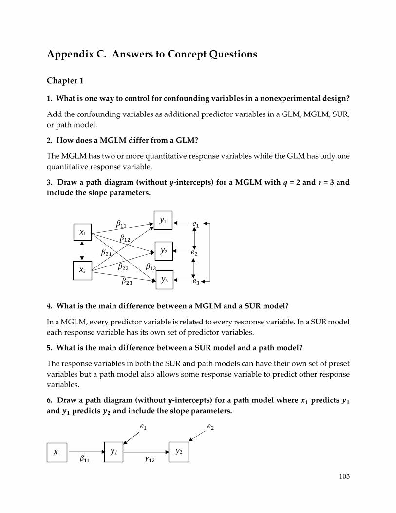
103

Appendix C. Answers to Concept Questions

Chapter 1

1. What is one way to control for confounding variables in a nonexperimental design?

Add the confounding variables as additional predictor variables in a GLM, MGLM, SUR,

or path model.

2. How does a MGLM differ from a GLM?

The MGLM has two or more quantitative response variables while the GLM has only one

quantitative response variable.

3. Draw a path diagram (without y-intercepts) for a MGLM with q = 2 and r = 3 and

include the slope parameters.

𝛽11 𝑒1

𝛽12

𝛽21 𝑒2

𝛽22 𝛽13

𝛽23 𝑒3

4. What is the main difference between a MGLM and a SUR model?

In a MGLM, every predictor variable is related to every response variable. In a SUR model

each response variable has its own set of predictor variables.

5. What is the main difference between a SUR model and a path model?

The response variables in both the SUR and path models can have their own set of preset

variables but a path model also allows some response variable to predict other response

variables.

6. Draw a path diagram (without y-intercepts) for a path model where 𝒙𝟏 predicts 𝒚𝟏

and 𝒚𝟏 predicts 𝒚𝟐 and include the slope parameters.

𝑒1 𝑒2

𝛽11 𝛾12 x1 y1 y2

x1

y1

y2

y3

x2

104

7. In a path model that predicts 𝒚𝟏 from 𝒙𝟏 and predicts 𝒚𝟐 from 𝒚𝟏, how is the indirect

effect of 𝒙𝟏 on 𝒚𝟐 defined?

If 𝛽11 is the path coefficient for 𝑥1 to 𝑦1 and 𝛾12 is the path coefficient for 𝑦1 to 𝑦2, then the

indirect effect from 𝑥1 to 𝑦2 is 𝛽11𝛾12.

8. How could you show that the population values of all included paths are

meaningfully large?

If the confidence interval for each included standardized path excludes 0 and each

confidence interval indicates that the standardized path is at least .25 in absolute value.

9. How could you show that the population values of all excluded paths in a SUR or

path model are small or unimportant?

If the confidence interval for each excluded standardized path indicates that the

standardized path is at most .25 in absolute value.

10. What can one conclude if the test for H0: B* = 0 is “significant”?

The result simply indicates that there is at least one predictor variable that has a nonzero

relation with at least one response variable.

11. What is the difference between a recursive path model and a nonrecursive path

model?

A nonrecursive model can have feedback paths and correlations among the prediction

errors.

12. If there are a total of 6 variables (predictor variables plus response variables), what

is the maximum number of slope and covariance parameters that can be estimated?

At most 6(7)/2 = 21 parameters can be estimated.

13. Why are modification indices useful?

They can be used to determine if any of the excluded paths are not small and should be

included in the model.

14. What are the assumptions for tests and confidence interval for unstandardized

slope coefficients in a GLM, MGLM, SUR model, or path model?

Random sample, independence among participants, normally distributed prediction

errors, homoscedastic predictor errors, and linear relations among all variables.

105

15. What are the assumptions for standardized slope confidence intervals?

Random sample, independence among participants, multivariate normality among all

variables.

16. Give the lavaan model specification for a GLM that predicts 𝒚𝟏 from 𝒙𝟏 and 𝒙𝟐.

model <- '

y1 ~ x1 + x2'

17. Give the lavaan model specification for a MGLM that predicts 𝒚𝟏 and 𝒚𝟐 from 𝒙𝟏

and 𝒙𝟐.

model <- '

y1 ~ x1 + x2

y2 ~ x1 + x2'

18. Give the lavaan model specification for a SUR model that predicts 𝒚𝟏 from 𝒙𝟏 and

predicts 𝒚𝟐 from 𝒙𝟏 and 𝒙𝟐.

model <- '

y1 ~ x1

y2 ~ x1 + x2'

19. Give the lavaan model specification for a path model that predicts 𝒚𝟏 from 𝒙𝟏 and

𝒙𝟐 and predicts 𝒚𝟐 from 𝒚𝟏.

model <- '

y1 ~ x1 + x2

y2 ~ y1'

20. Give the lavaan model specification for a path model that predicts 𝒚𝟏 from 𝒙𝟏 and

predicts 𝒚𝟐 from 𝒚𝟏. Include the specification for the indirect effect of 𝒙𝟏 on 𝒚𝟐.

model <- '

y1 ~ b11*x1

y2 ~ g12*y1

ind := b11*g12'

Chapter 2

1. What is the effect of measurement error in y and x on 𝝆𝒚𝒙?

Measurement error in y or x will attenuate the correlation between y and x.

2. What is the effect of measurement error in x on 𝜷𝟏 in a simple linear regression

model?

Measurement error in x will attenuate the slope coefficient.

106

3. What is the effect of measurement error in y on the confidence intervals for 𝜷𝟏 in a

simple linear regression model?

Measurement error in y will not attenuate the slope coefficient but will increase the

standard error of the slope estimate.

4. Explain the difference between the strictly parallel and parallel measurement

models.

The strictly parallel model assumes equal means of the measurements, equal factor

loadings, and equal unique factor variances. The parallel model assumes equal factor

loadings and equal unique factor variances but not equal means.

5. Explain the difference between the parallel and tau-equivalent measurement

models.

The parallel model assumes equal factor loadings and equal unique factor variances. The

tau-equivalent model assumes equal unique factor variances and does not assume equal

factor loadings or equal means of the measurements.

6. Explain the difference between the tau-equivalent and congeneric measurement

models.

The tau-equivalent assumes equal unique factor variances. The congeneric model does

not assume equal unique factor variances (or equal factor loadings or equal means).

7. Why are standardized factor loadings useful?

Standardized factor loadings describe the standard deviation change in an indicator

variable associated with 1-point increase in 𝑒𝜂𝑗 where 𝑒𝜂𝑗

is the component of 𝜂𝑗 that is

unrelated to all other factors in the model. If the factors are uncorrelated then 𝑒𝜂𝑗= 𝜂𝑗 and

then the standardized loading is equal to a Pearson correlation.

8. What is the maximum number of parameters that can be uniquely estimated in a

factor analysis model with r = 5 observed variables?

5(6)/2 = 15

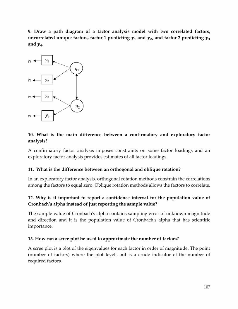
107

9. Draw a path diagram of a factor analysis model with two correlated factors,

uncorrelated unique factors, factor 1 predicting 𝒚𝟏 and 𝒚𝟐, and factor 2 predicting 𝒚𝟑

and 𝒚𝟒.

e1

e2

e3

e4

10. What is the main difference between a confirmatory and exploratory factor

analysis?

A confirmatory factor analysis imposes constraints on some factor loadings and an

exploratory factor analysis provides estimates of all factor loadings.

11. What is the difference between an orthogonal and oblique rotation?

In an exploratory factor analysis, orthogonal rotation methods constrain the correlations

among the factors to equal zero. Oblique rotation methods allows the factors to correlate.

12. Why is it important to report a confidence interval for the population value of

Cronbach’s alpha instead of just reporting the sample value?

The sample value of Cronbach's alpha contains sampling error of unknown magnitude

and direction and it is the population value of Cronbach's alpha that has scientific

importance.

13. How can a scree plot be used to approximate the number of factors?

A scree plot is a plot of the eigenvalues for each factor in order of magnitude. The point

(number of factors) where the plot levels out is a crude indicator of the number of

required factors.

𝑦1

𝑦2

𝑦3

𝑦4

𝜂1

𝜂2

108

14. Why are structure and standardized pattern matrices the same with orthogonal

rotation?

A standardized factor loading simplifies to a correlation between the factor and the

indicator when the factors are uncorrelated.

15. When would ULS estimates be preferred to ML estimates?

In small samples

16. How can model modification indices be used in a CFA?

The omitted factor loading with the largest modification index can be added to the model

and a confidence interval for the added loading can be used to decide if that loading

should be included in the model. This same approach can be used for omitted correlations

among factors and unique factors.

17. Why is a confidence interval for 𝝀𝟏 – 𝝀𝟐 more informative that a test of H0: 𝝀𝟏 = 𝝀𝟐?

A confidence interval for 𝜆1 – 𝜆2 can be used to determine both the direction and the

magnitude of the difference while a test can only determine the direction of the difference.

18. When would you consider using robust standard errors?

When approximate multivariate normality is not plausible.

19. When would McDonald’s reliability coefficient be preferred to Cronbach’s

reliability coefficient?

When the factor loadings of a 1-factor CFA are highly dissimilar

20. How could you show that the population error variances for three measures of

some attributes are similar?

Compute confidence intervals for all pairwise ratios of variances (or standard deviations).

21. How could you show that the population factor loadings for three measures of

some attributes are similar?

Compute confidence intervals for all pairwise differences in standardized factor loadings.

109

22. How could you show that the omitted population factor loadings in a CFA are

small or unimportant?

If the confidence interval for the omitted factor loading with the largest modification

index is small when added to the model, then it is likely that all other omitted factor

loadings are also small and need not be added to the model.

23. How could you show that the included population factor loadings in a CFA are

meaningfully large?

Compute confidence intervals for all standardized factor loadings and show that all

loadings are greater than .4 in absolute value.

24. Explain how fit indices can be misused.

A "good" fit index value does not guarantee that all omitted parameters are small, and a

"poor" fit index value does not necessary mean that some omitted parameters are large.

25. Give the lavaan model specification for a strictly parallel measurement model.

model <- '

f ~= lamda*I1 + lamda*I2 + lamda*I3 + lamda*I4

I1 ~~ var*I1

I2 ~~ var*I2

I3 ~~ var*I3

I4 ~~ var*I4

I1 ~ mean*1

I2 ~ mean*1

I3 ~ mean*1

I4 ~ mean*1 '

26. Modify the above lavaan model specification to define a parallel measurement

models and include a new parameter equal to Cronbach's reliability coefficient.

model <- '

f ~= lamda*I1 + lamda*I2 + lamda*I3 + lamda*I4

I1 ~~ var*I1

I2 ~~ var*I2

I3 ~~ var*I3

I4 ~~ var*I4

rel := (4*lambda)^2/(4*lambda)^2 + 4*var)'

27. Give the lavaan model specification for a congeneric measurement model.

model <- '

f ~= I1 + I2 + I3 + I4 '

110

Chapter 3

1. What is the benefit of using a latent predictor variable?

Latent predictor variables have less measurement error which leads to less bias in the

slope coefficients.

2. What is the benefit of using a latent response variable?

Latent response variables have less measurement error which leads to smaller standard

errors of the slope coefficients estimates.

3. What is the effect of measurement error on indirect effects?

Measurement error in x and the mediator variable will bias the path coefficients.

Measurement error in the mediator and response variables will inflate the standard

errors.

4. Why is baseline centering often used in latent growth curve models?

With baseline centering, the intercept factor mean represents the mean of the response

variable at the first time period.

5. Explain how goodness of fit tests are misused.

Researchers incorrectly interpret a nonsignificant GOF test as evidence that all of the

omitted model parameters are small, and incorrectly interpret a significant GOF test as

evidence that some of the omitted parameters are large.

6. What is the effect of kurtosis on the GOF test statistic and standard errors?

With leptokurtosis, the standard errors are too small and the GOF p-value is too large.

With platykurtosis, the standard errors are too large and the GOF p-value is too small.

7. How could you show that the included paths in a latent variable path model are

meaningfully large.

Compute confidence intervals for all included standardized paths.

8. How could you show that the omitted paths in a latent variable path model are small

or unimportant?

111

If a confidence interval for the omitted path with the largest modification index is small

when added to the model, then it is likely that all other omitted paths are also small and

need not be added to the model.

9. When would you consider using a bootstrap confidence intervals?

If approximate multivariate normality is not plausible

10. How can interaction effects be estimated in a multiple group model?

A difference in slope coefficients between two groups defines an interaction effect.

11. When would you use a latent variable growth curve model in lavaan rather than a

mixed model program in SPSS or SAS?

If any of the time-varying or time-invariant predictor variables are latent variables then

latent growth curve is needed.

12. What is the advantage of using an ANCOVA model with latent covariates over the

traditional ANCOVA?

Observed covariates with low reliabilities are not as effective in removing confounding

variable bias as latent covariates.

13. Why is it important to discuss equivalent models when reporting the results of a

particular model?

Different equivalent models, which are equally plausible on the basis of statistical criteria

such as fit indices of GOF tests, can have very different theoretical interpretations and

implications.

14. Give the lavaan model specification code for a MGLM with two latent predictor

variables, two latent responses variables, with all latent variables having two

indicators.

model <- '

f1 ~= lam1*x1 + lam1*x2

f2 ~= lam2*x3 + lam2*x4

f3 ~= 1*y1 + l*y2

f4 ~= 1*y3 + 1*y4

f3 ~ f1 + f2

f4 ~ f1 + f2 '

112

15. Give the lavaan model specification code for a path model where two latent

predictor variables predict one latent mediator variable which predicts an observed

response variable. The two latent predictor variables each have three indicators and

the latent mediator variable has two indicators.

model <- '

f1 ~= l*x1 + x2 + x3

f2 ~= l*x4 + x5 + x6

f3 ~= l*y1 + 1*y2

f3 ~ f1 + f2

y3 ~ f3 '

16. Give the lavaan model specification code for a latent growth curve model with three

time periods where 𝝃𝟏 predicts the latent intercept and the latent slope, and 𝒙𝟏 and 𝒙𝟐

are tau-equivalent indicators of 𝝃𝟏.

model <- '

f1 ~= l*x1 + 1*x2

int ~= l*y1 + 1*y2 + 1*y3

slope ~= 0*y1 + 1*y2 + 2*y3

int ~ f1

slope ~ f1 '

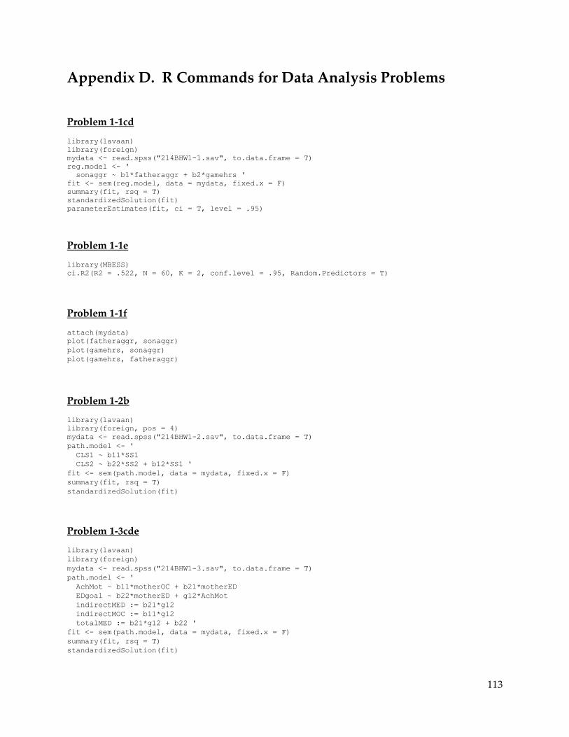
113

Appendix D. R Commands for Data Analysis Problems

Problem 1-1cd

library(lavaan)

library(foreign)


reg.model <- '

sonaggr ~ b1*fatheraggr + b2*gamehrs '

fit <- sem(reg.model, data = mydata, fixed.x = F)




Problem 1-1e

library(MBESS)

ci.R2(R2 = .522, N = 60, K = 2, conf.level = .95, Random.Predictors = T)

Problem 1-1f

attach(mydata)

plot(fatheraggr, sonaggr)

plot(gamehrs, sonaggr)

plot(gamehrs, fatheraggr)

Problem 1-2b

library(lavaan)

library(foreign, pos = 4)


path.model <- '

CLS1 ~ b11*SS1

CLS2 ~ b22*SS2 + b12*SS1 '

fit <- sem(path.model, data = mydata, fixed.x = F)



Problem 1-3cde

library(lavaan)

library(foreign)


path.model <- '

AchMot ~ b11*motherOC + b21*motherED

EDgoal ~ b22*motherED + g12*AchMot

indirectMED := b21*g12

indirectMOC := b11*g12

totalMED := b21*g12 + b22 '

fit <- sem(path.model, data = mydata, fixed.x = F)



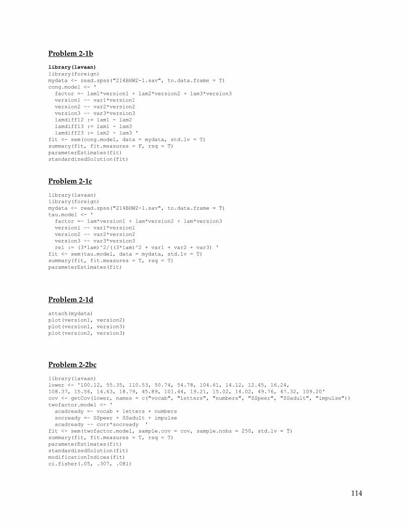
114

Problem 2-1b

library(lavaan)

library(foreign)


cong.model <- '

factor =~ lam1*version1 + lam2*version2 + lam3*version3

version1 ~~ var1*version1





lamdiff23 := lam2 - lam3 '


summary(fit, fit.measures = F, rsq = T)

parameterEstimates(fit)


Problem 2-1c

library(lavaan)

library(foreign)


tau.model <- '

factor =~ lam*version1 + lam*version2 + lam*version3




rel := (3*lam)^2/((3*lam)^2 + var1 + var2 + var3) '


summary(fit, fit.measures = T, rsq = T)


Problem 2-1d

attach(mydata)

plot(version1, version2)



Problem 2-2bc

library(lavaan)

lower <- '100.12, 55.35, 110.53, 50.74, 54.78, 104.61, 14.12, 12.45, 16.24,

108.37, 15.56, 14.63, 18.79, 45.89, 101.44, 19.21, 15.02, 14.02, 49.76, 47.32, 109.20'

cov <- getCov(lower, names = c("vocab", "letters", "numbers", "SSpeer", "SSadult", "impulse"))


acadready =~ vocab + letters + numbers

socready =~ SSpeer + SSadult + impulse

acadready ~~ corr*socready '

fit <- sem(twofactor.model, sample.cov = cov, sample.nobs = 250, std.lv = T)




modificationIndices(fit)

ci.fisher(.05, .307, .081)

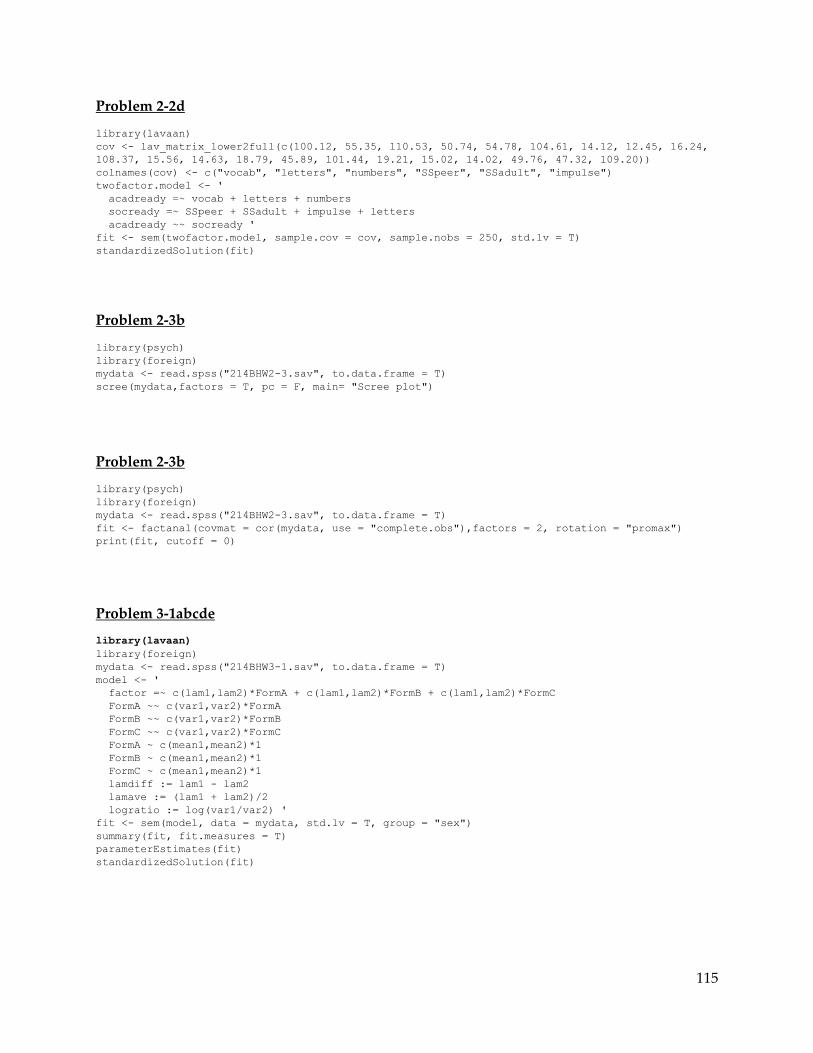
115

Problem 2-2d

library(lavaan)

cov <- lav_matrix_lower2full(c(100.12, 55.35, 110.53, 50.74, 54.78, 104.61, 14.12, 12.45, 16.24,

108.37, 15.56, 14.63, 18.79, 45.89, 101.44, 19.21, 15.02, 14.02, 49.76, 47.32, 109.20))

colnames(cov) <- c("vocab", "letters", "numbers", "SSpeer", "SSadult", "impulse")


acadready =~ vocab + letters + numbers

socready =~ SSpeer + SSadult + impulse + letters

acadready ~~ socready '

fit <- sem(twofactor.model, sample.cov = cov, sample.nobs = 250, std.lv = T)


Problem 2-3b

library(psych)

library(foreign)


scree(mydata,factors = T, pc = F, main= "Scree plot")

Problem 2-3b

library(psych)

library(foreign)


fit <- factanal(covmat = cor(mydata, use = "complete.obs"),factors = 2, rotation = "promax")

print(fit, cutoff = 0)

Problem 3-1abcde

library(lavaan)

library(foreign)


model <- '

factor =~ c(lam1,lam2)*FormA + c(lam1,lam2)*FormB + c(lam1,lam2)*FormC

FormA ~~ c(var1,var2)*FormA

FormB ~~ c(var1,var2)*FormB

FormC ~~ c(var1,var2)*FormC

FormA ~ c(mean1,mean2)*1

FormB ~ c(mean1,mean2)*1

FormC ~ c(mean1,mean2)*1

lamdiff := lam1 - lam2

lamave := (lam1 + lam2)/2

logratio := log(var1/var2) '

fit <- sem(model, data = mydata, std.lv = T, group = "sex")

summary(fit, fit.measures = T)



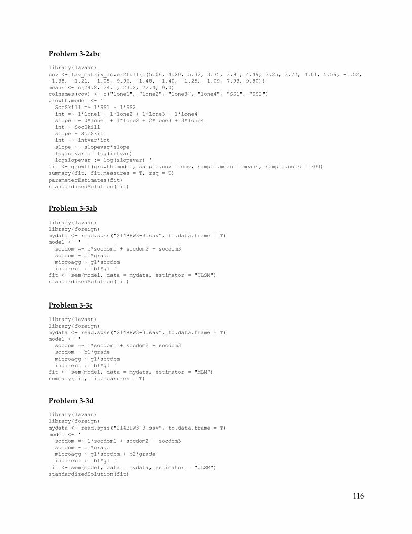
116

Problem 3-2abc

library(lavaan)

cov <- lav_matrix_lower2full(c(5.06, 4.20, 5.32, 3.75, 3.91, 4.49, 3.25, 3.72, 4.01, 5.56, -1.52,

-1.38, -1.21, -1.05, 9.96, -1.48, -1.40, -1.25, -1.09, 7.93, 9.80))

means <- c(24.8, 24.1, 23.2, 22.4, 0,0)

colnames(cov) <- c("lone1", "lone2", "lone3", "lone4", "SS1", "SS2")

growth.model <- '

SocSkill =~ 1*SS1 + 1*SS2

int =~ 1*lone1 + 1*lone2 + 1*lone3 + 1*lone4

slope =~ 0*lone1 + 1*lone2 + 2*lone3 + 3*lone4

int ~ SocSkill

slope ~ SocSkill

int ~~ intvar*int

slope ~~ slopevar*slope

logintvar := log(intvar)

logslopevar := log(slopevar) '

fit <- growth(growth.model, sample.cov = cov, sample.mean = means, sample.nobs = 300)




Problem 3-3ab

library(lavaan)

library(foreign)


model <- '

socdom =~ 1*socdom1 + socdom2 + socdom3

socdom ~ b1*grade

microagg ~ g1*socdom

indirect := b1*g1 '

fit <- sem(model, data = mydata, estimator = "ULSM")


Problem 3-3c

library(lavaan)

library(foreign)


model <- '


socdom ~ b1*grade

microagg ~ g1*socdom

indirect := b1*g1 '

fit <- sem(model, data = mydata, estimator = "MLM")

summary(fit, fit.measures = T)

Problem 3-3d

library(lavaan)

library(foreign)


model <- '


socdom ~ b1*grade

microagg ~ g1*socdom + b2*grade

indirect := b1*g1 '

fit <- sem(model, data = mydata, estimator = "ULSM")


Date post:	28-Jan-2022
Category:	Documents
Upload:	others
View:	25 times
Download:	0 times

An Introduction to Multivariate Statistical Models

Documents