An Introduction to Stability Theory for Nonlinear PDEs Mathew A. Johnson 1 Abstract These notes were prepared for the 2017 Participating School in Analysis of PDE: Stability of Solitons and Periodic Waves held in KAIST in Daejeon, Korea during August 21 - August 25, 2017. Their main focus is to introduce participants to some of the basic methodologies and techniques for obtaining spectral, linear and nonlinear stability results for nonlinear wave solutions to special classes of PDEs, with explicit examples being worked out whenever possible. Contents 1 Introduction 2 2 Spectral Theory: Survey of Results 5 2.1 BVP with Separated Boundary Conditions .................. 6 2.2 Exponentially Localized Coefficients ...................... 8 2.3 Periodic Coefficients ............................... 10 2.3.1 Periodic Boundary Conditions ..................... 11 2.3.2 Acting on Whole Line .......................... 12 3 Linear Dynamics and Stability 13 3.1 Dynamics Induced by the Spectrum ...................... 14 3.2 Examples ..................................... 16 3.2.1 Reaction Diffusion on Bounded Domain ................ 16 3.2.2 Stationary Pulse of Reaction Diffusion Equation ........... 17 3.2.3 Stationary Front in Reaction Diffusion Equation ........... 18 3.2.4 The KdV Equation ............................ 19 3.3 Linear Stability .................................. 20 3.4 Linear Stability of Monotone Front ....................... 23 3.5 The Periodic Case ................................ 24 4 Nonlinear Stability: Examples 25 4.1 Reaction Diffusion on Bounded Domain .................... 25 4.2 Reaction Diffusion: Stationary Front ...................... 29 4.3 Discussion of the Periodic Case ......................... 36 1 Department of Mathematics, University of Kansas. E-mail: [email protected]1
Transcript
An Introduction to Stability Theory for Nonlinear PDEs
Mathew A. Johnson1
Abstract
These notes were prepared for the 2017 Participating School in Analysis of PDE:Stability of Solitons and Periodic Waves held in KAIST in Daejeon, Korea during August21 - August 25, 2017. Their main focus is to introduce participants to some of thebasic methodologies and techniques for obtaining spectral, linear and nonlinear stabilityresults for nonlinear wave solutions to special classes of PDEs, with explicit examplesbeing worked out whenever possible.
1Department of Mathematics, University of Kansas. E-mail: [email protected]
1
1 Introduction
The purpose of this summer school is to introduce students and early career researchersto various aspects of the stability theory for special classes of solutions in some importantnonlinear partial differential equations (PDEs). Many times, this theory mimics classicalfinite-dimensional ODE theory, while making appropriate modifications accounting for thefact that the state space for PDEs is inherently infinite dimensional. Consequently, we willbegin with a very brief review of finite-dimensional ODE stability theory.
To begin, consider a nonlinear ODE of the form
u = F (u), u = u(t) ∈ Rn (1)
where here F : Rn → Rn is sufficiently smooth and u refers to the derivative of u withrespect to the dependent variable t. Basic results in ODE theory guarantee that for eachinitial condition u0 ∈ Rn, there will exist a unique solution u(t;u0) of (1) with u(0;u0) = u0
that exists at least locally, i.e. for at least |t| � 1. The basic question in stability theory isthe following:
Question: If u0 ∈ Rn is a fixed point of F , so that F (u0) = 0, and if |u1 − u0| � 1, willu(t;u1) remain near u0 for all t > 0? If not, what happens?
Observe that by continuous dependence, we know that since |u1 − u0| � 1 we will have|u(t;u1)−u0| � 1 for at least a short amount of time. A natural and often used method todetermine if u(t;u1) stays close to u0 for all time t > 0 is to first approximate the dynamicsof (1) near u0 by studying a suitable approximating system. This leads to the process oflinearization.
To this end, note that we may write, for so long as it exists,
u(t;u1) = u0 + v(t)
so that now u(t;u1) is considered as a perturbation of u0. From (1), the function v(t) solvesthe initial value problem (IVP)
v = F (u0 + v), v(0) = u1 − u0 (2)
Noting that we can write
F (u0 + v) = F (u0) +DF (u0)v + (F (u0 + v)− F (u0)−DF (u0))︸ ︷︷ ︸O(|v|2)
,
where here DF is the n × n matrix valued derivative of F at u0, it follows v satisfies anIVP of the form
v = DF (u0)v +O(|v|2), v(0) = u1 − u0, (3)
2
where we have used here the fact that F (u0) = 0 by construction. Using Duhamel’s formulaor, equivalently, variation of parameters, we can rewrite the above evolution equation forthe perturbation v as the implicit integral equation
v(t) = eDF (u0)tv(0) +
∫ t
0eDF (u0)(t−s)O(|v(s)|2)ds
where here eDF (u0)t is the n × n matrix exponential of the linear operator DF (u0). Inparticular, for every v(0) ∈ Rn the vector eDF (u0)tv(0) is the unique solution to the linearsystem
v = DuF (u0)v, v(0) = u1 − u0. (4)
Since the O(|v|2) are small compared to the DuF (u0)v terms when v is small, we expect thatso long as |v(t)| remains small that solutions of (2) will be well approximated by solutionsof (4), the solutions of which are governed completely by the eigenvalues of the matrixDF (u0). In particular, if λ is an eigenvalue of DF (u0) with eigenfunction w ∈ Rn then thefunction v(t) = eλtw is a solution of (4). It follows that if all the eigenvalues of DF (u0)have strictly negative real part, then all the solutions of (4) decay exponentially as t→∞,while if there is any eigenvalue with positive real part then there exists some solution of(4) that blows up as t → ∞. Finally, if DF (u0) has an eigenvalue on the imaginary axisiR, then (4) has a solution that remains bounded for all t ∈ R, being oscillatory and notdecaying for large time.
A natural question, and one of the key problems in classical ODE stability theory, iswhen the predictions from the linearized system (4) carry over to the nonlinear system(3). In classical ODE theory, the simplest result in this direction is the Stable ManifoldTheorem. To motivate this result, suppose for a moment that all eigenvalues of DF (u0) aresemisimple, i.e. their algebraic multiplicity agrees with their geometric multiplicity (so noJordan blocks). Then we can express
eLt =k∑j=1
eλjtΠj
where the Πj are the spectral projections onto the eigenspaces associated with the k distincteigenvalues of DF (u0). It follows that if ω = maxj <(λj) then there exists a constant C > 0such that ∣∣eLt∣∣ ≤ Ceωtfor all t > 0. In particular if <(λj) < −γ for some constant γ > 0 and all j then everysolution of (4) will satisfy |v(t)| ≤ Ce−γt|v(0)| for all t > 0. The fact that this observationcarries over for the nonlinear equation (3), even when DF (u0) may admit Jordan blocks,follows by the following fundamental result.
Theorem 1 (Stable Manifold Theorem). Suppose there exists a constant γ > 0 such thatevery eigenvalue λ ∈ C of the matrix DF (u0) satisfies <(λ) < −γ. Then there exists
3
constants δ > 0 and C ≥ 1 such that if |v0| < δ then the associated unique solution v(t) of(3) exists for all t > 0 and satisfies the exponential decay estimate
|v(t)| ≤ Ce−γt|v(0)|
for all t ≥ 0. In particular, u0 is an asymptotically stable solution of (1).
Remark 1. By essentially taking t→ −t in the proof of the Stable Manifold Theorem, onecan show that if DF (u0) has an eigenvalue with strictly positive real part, then u0 is anunstable solution of (1): there exists an ε > 0 such that for every δ ∈ (0, ε) there existsinitial data v(0) with |v(0)| < δ such that the associated solution v(t) satisfies |v(T )| > εfor some finite T > 0. This result is known as the Unstable Manifold Theorem
Remark 2. We note that if DF (u0) has an eigenvalue on the imaginary axis, one must workharder in order to determine the stability of u0: it may be stable or unstable depending onthe particular nonlinearity. In this case, one usually either uses a center manifold reduction,or tries the study the stability of u0 through energy (i.e. Lyapunov) methods instead.
In these notes, we are interested in extending the above results to be suitable for PDEapplications. Some of the initial challenges include:
(1) In the PDE case, establishing that the PDE can be solved, even locally in time, forinitial data “near” the background wave u0 is a much more delicate matter. One thingthat complicates this is evolutionary PDE’s of the form ut = F (u), where here F maybe a nonlinear differential operator with possibly non-constant coefficients, describethe evolution of functions in infinite dimensional vector spaces. Consequently, thereare many non-equivalent topologies one may use to define what “close” means, andidentifying the appropriate topology in which to work is not always easy.
(2) The linearized operator DF (u0) is now generally a differential operator with coeffi-cients depending on the function u0. Describing the spectral properties of DF (u0)then takes significantly more care, since linear operators on infinite dimensional vectorspaces may fail to be invertible in more ways than losing injectivity, i.e. there maybemore than eigenvalues we have to worry about. Such issues are discussed in Section2 below. Furthermore, turning spectral properties into decay bounds on the linearsolution operator2 eLt also becomes a much more delicate matter, and is discussed inSection 3.3.
(3) In PDE’s modeling extended systems, i.e. defined on the infinite line R, the linearizedoperator often does not have a spectral gap, i.e. the spectrum of DF (u0) includespoints on the imaginary axis. This is often due to the presence of continuous symme-tries in the governing PDE, such as the PDE being translationally invariant, whichcauses the linearized operator DF (u0) to fail to be invertible: see Remark 6 in Section
2In fact, since differential operators are unbounded from spaces into themselves, it is not a-priori clearhow to even define eLt.
4
3.2.2. Dealing with this lack of spectral gap is an important matter, and somethingthat is fundamental to the stability analysis of PDE’s. We will discuss some methodsin this direction in Section 4.2 and Section 4.3 below.
Acknowledgments: I would like to thank Soonsik Kwon for organizing such a wonderfulsummer school workshop at KAIST, and for inviting me to be a mentor for the participantsinvolved. I am also grateful to Kihyun Kim for pointing out many typos in the originalversion of these notes. These notes were written while the author was supported by NSFgrant DMS-1614785.
Disclaimer: These notes were extracted from a class I taught during the Fall 2015 semesterat the University of Kansas. The primary text for that course was the book [KP] by ToddKapitula and Keith Promislow. As such, while these notes do not follow [KP] verbatim,they were heavily influenced it. Most everything in these notes can be found in [KP], and,due to time constraints when writing these notes, I make no attempt to flush out precisepage or theorem number references. Also, there are hundreds of additional references thatshould be cited throughout these notes, but for the same reasons they are not listed here.My apologies to all those who should be cited, and to anyone reading these notes.
2 Spectral Theory: Survey of Results
In this section, we briefly discuss the relevant definitions from spectral theory. We will thendiscuss the nature of the spectrum for classes of differential operators that arise naturallyin stability theory for nonlinear waves.
Consider an nth-order, scalar linear differential operator of the form
L = ∂nx + an−1(x)∂n−1x + an−2(x)∂n−2
x + . . .+ a1(x)∂x + a0(x) (5)
where here the functions aj are sufficiently smooth. In PDE applications, such operatorsarise naturally as the linearizations of a PDE about a some nonlinear wave solution, wherethe coefficient functions aj depend on the background wave. Since for this workshop we areinterested in the stability of solitary and periodic waves, we will briefly discuss the spectralproperties of operators of the form L in when the aj are either exponentially localized orspatially periodic, corresponding to the cases when L is the linearization about a solitaryor periodic wave, respectively.
We begin with some basic definitions.
Definition 1. Suppose L acts on a complex Banach space X. The resolvent set of L onX, denoted by ρ(L) is the set of all λ ∈ C where L − λI is invertible with bounded (i.e.continuous) inverse. Here, I denotes the identity operator. Further, the spectrum of L onX, denoted σ(L) is defined as σ(L) := C \ ρ(L). Finally, the λ ∈ σ(L) is an eigenvalue ofL if Ker(L− λI) 6= {0}, i.e. if there exists a v ∈ X \ {0} such that Lv = λv..
5
Remark 3. Note the choice of the Banach space X on which L acts is crucial in ourunderstanding of the the spectrum of L. As we will see below, the spectral properties of agiven operator can change dramatically if one changes the space X.
In many applications, it is useful to further decompose the spectrum of L. There areseveral non-equivalent ways of doing this, all of which appear in the literature. For thepurpose of this lecture, we will use the following definition.
Definition 2. Given a linear operator L acting on a complex Banach space X as above,the point spectrum of L, denoted σp(L) (on X) is the set of all isolated eigenvalues of L (onX) with finite multiplicities. Further, the essential spectrum is σess(L) := σ(L) \ σp(L).
As we will see, in stability theory the point and essential spectrum give drasticallydifferent information concerning the dynamics near a given nonlinear wave. In what fol-lows, we discuss spectral properties for classes of differential operators often occurring inapplications, as well as how the spectrum may be calculated.
2.1 BVP with Separated Boundary Conditions
First, let’s consider a differential operator of the form
L = ∂2x + a1(x)∂x + a0(x) (6)
where a0, a1 are some given smooth, real-valued functions and let T > 0 be finite. Considerthe spectral problem
Lv = λv, x ∈ (−T, T ) (7)
equipped with homogeneous Dirichlet boundary conditions
v(−T ) = v(T ) = 0. (8)
Precisely, we are considering L as a densely defined operator on L2(−T, T ) with denselydefined domain D(L) := H1
0 (T, T ) ∩H2(−T, T ). Our goal here is to characterize σ(L).Our first observation is that the operator L is self-adjoint with respect to the weighted
inner product
〈f, g〉 :=
∫ T
−Tf(x)g(x)ρ(x)dx,
where the weight function is ρ(x) := exp(∫ x
0 a1(z)dz). Consequently, σ(L) ⊂ R.
Next, we search for eigenvalues of L, i.e. we search for λ ∈ C such that there exists anon-trivial solution of (7) satisfying the B.C.’s at ±T . To this end, let φ± be the uniquesolutions of the IVP
Lv = λv, x ∈ (−T, T )
v(±T ) = 0
v′(±T ) = 1
6
and note that for each λ ∈ C the function φ−(·;λ) satisfies the B.C. at x = −T , while thefunction φ+(·;λ) satisfies the B.C. at x = T . Observe that if φ± are linearly dependent forsome λ ∈ C, then there exists a constant C > 0 such that
φ−(x;λ) = Cφ+(x;λ) ∀x ∈ [−T, T ]
so that, in particular, the function φ+ provides a non-trivial solution of (7) satisfying bothboundary conditions at x = ±T , and hence λ ∈ σp(L). Note if we define the Wronskian3
E(λ) := det
(φ+(x;λ) φ−(x;λ)φ′+(x;λ) φ′−(x;λ)
)then the functions φ±(·;λ) are linearly dependent precisely on the zero set of E. It can beeasily checked that E(λ) is an entire function of λ, and that the multiplicity of λ as a rootof E agrees with the algebraic multiplicity of λ as an eigenvalue of L. By basic results incomplex analysis, it follows that the eigenvalues of L are isolated with no finite accumulationpoint, and all eigenvalues necessarily have finite algebraic (and hence geometric) multiplicity.
Remark 4. Note that if L has constant coefficients a1, a0 ∈ R then σp(L) can be foundthrough elementary ODE techniques. Indeed, for every λ ∈ C one can write the generalsolution to the second-order ODE Lv = λv and determine for which λ this solution satisfiesthe appropriate boundary conditions.
Next, I claim that if λ /∈ σp(L) then λ ∈ ρ(L). To see this, note that if E(λ) 6= 0 thenφ±(·;λ) provides two linearly independent solutions of the 2nd order homogeneous ODELv + λv = 0. Given any f ∈ L2(−T, T ), one can now show that the unique solution v ofthe equation
Lv − λv = f
that satisfies the B.C.’s (8) at ±T is given explicitly by
v(x;λ) =φ+(x;λ)
E(λ)
∫ x
−Tf(z)φ−(z;λ)dz +
φ−(x;λ)
E(λ)
∫ T
xf(z)φ+(z;λ)dz
=
∫ T
−TG(x, z;λ)f(z)dz,
where G here is the Green’s function, given explicitly as
where χ(a,b) denotes the characteristic function of the set (a, b). Since a simple applicationof Holder’s inequality implies that
‖v(x;λ)‖L2(−T,T ) ≤ C(λ)‖f‖L2(−T,T ),
3It is easily checked that the determinant defining E(λ) is independent of x. However, in applicationsit is sometimes helpful to have the flexibility in choosing at what x ∈ [−T, T ] to do the evaluation. Thisfunction E(λ) can also be identified as the so-called “Evans function” for the given boundary value problem.
7
for all λ ∈ C with E(λ) 6= 0, i.e. λ /∈ σp(L), it follows that (L− λI)−1 is a bounded linearoperator on L2(−T, T ), and hence that λ ∈ ρ(L), as claimed.
It is important to note that the fact that σ(L) = σp(L) in the above example holds inmuch more generality. Indeed, it holds for general nth-order linear differential operatorsdefined bounded intervals [a, b] ⊂ R, when equipped with n separated boundary conditionsat x = a and x = b. It can even be seen to hold in higher dimensions through the use ofthe Rellich-Kondrachov compactness theorem. The fact that σ(L) ⊂ R does not generallyextend to such operators, but holds here due to the fact that the second-order operator Lis a Sturm-Liouville operator. Furthermore, using the fact that L is second order, we havethe following version of Sturm’s Oscillation Theorem that is often helpful in studying σp(L)in such cases.
Theorem 2 (Sturm’s Oscillation Theorem for BVP’s with Separated Boundary Condi-tions). Let L be a second-order, linear differential operator of the form (6), considered asan operator on L2(a, b) with separated boundary conditions at x = a and x = b. Then σp(L)consists of infinitely many simple eigenvalues which can be numerated in strictly decreasingorder as
λ0 > λ1 > λ2 > . . . , limn→∞
λn = −∞.
Further, an eigenfunction associated with λj has exactly j zeroes on (a, b), all of which aresimple.
2.2 Exponentially Localized Coefficients
Next, we consider the case when the functions aj are exponentially localized in space, i.e.there exists an r > 0 and constants a0, a1 . . . , an−1 ∈ R such that
limx→∞
er|x||aj(x)− aj | = 0
for all j = 0, 1, 2, . . . , n − 1. Here, we consider L as acting on the Lebesgue space L2(R)with densely defined domain Hn(R) (a Sobolev space). Such operators arise naturally whenlinearizing a PDE defined on all of R about a wave that is asymptotically constant, such asa solitary wave or a front. We first discuss the essential spectrum of L. The key result hereis known as the Weyl Essential Spectrum Theorem which, in this context, roughly statesthat the essential spectrum of L is controlled entirely by the behavior of the operator atspatial infinity. To make this precise, define the constant-coefficient asymptotic operator
L∞ := ∂nx + an−1∂n−1x + . . .+ a1∂x + a0
We then have the following key result.
Theorem 3 (Weyl Essential Spectrum Theorem). With L and L∞ as above, we have
σess(L) = σess(L∞).
8
The proof of this theorem relies on the fact that since the coefficient functions aj(x)of L are exponentially localized, the operator L is a relatively compact perturbation of theoperator L∞. Since functional analysis tells us the essential spectrum of an operator isinvariant under relatively compact perturbations, the result follows.
Remark 5. In the case where the functions aj are exponentially localized to different limit-ing values a±1 , a
±0 at ±∞, such as what appears when linearizing a PDE about a front solu-
tion, the essential spectrum of L may then be a subset of C with non-zero two-dimensionalmeasure. Consequently, Weyl’s Essential Spectrum Theorem becomes more complicated inthat scenario. Nevertheless, if we define asymptotic operators L±∞ at x = ±∞, respec-tively, one can show that the one-dimensional curves σess(L−∞) and σess(L+∞), known asthe “Fredholm boundaries” of L, form the boundary of the essential spectrum of L. Most im-portantly for stability purposes, if the essential spectrum for both asymptotic operators L±∞lies in the left half plane, then the essential spectrum of L also lies in the left half plane.Consequently, for stability purposes it is enough to just calculate the Fredholm boundaries.
It remains to determine how to calculate the essential spectrum for the constant coef-ficient operator L∞ on L2(R). Thankfully, this is actually very simple! Indeed, define thepolynomial p(z) = zn + an−1z
n−1 + . . . a0 so that L∞ = p(∂x): the polynomial p is calledthe symbol of L. For a given λ ∈ C, we now try to solve the equation (L − λI)v = w fora given w ∈ L2(R). Since this equation has constant coefficients, this is easily solved usingthe Fourier transform. Indeed, denoting the Fourier transform of a function v ∈ L2(R) as
F(v)(ξ) = v(ξ) :=1√2π
∫Re−iξxv(x)dx
and noting that ∂mx v(ξ) = (−iξ)mv(ξ) for all positive integers m, it follows that
Clearly, since ξ ∈ R, if λ ∈ p(iR) one can find a w ∈ L2(R) such that the function v definedabove is not in L2(R). Consequently, (L− λI)−1 is not well defined on all of L2(R) for anyλ ∈ p(iR). Furthermore, if λ /∈ p(iR) then the above defines a unique solution v ∈ Hn(R)for each w ∈ L2(R). Indeed, the Parseval inequality implies that for λ /∈ p(iR) we have thebound ∥∥∥(L− λI)−1 (w)
∥∥∥Hn(R)
≤n∑j=0
(∥∥∥∥ (i·)j
p(i·)− λ
∥∥∥∥L∞(R)
)‖w‖L2(R),
which implies that λ ∈ ρ(L). Combining these insights with the Weyl Essential SpectrumTheorem, it follows that for a differential operator L of the form (5), one has
σess(L) = p(iR)
where p(z) is the symbol of the constant coefficient, asymptotic operator L∞.
9
While the essential spectrum in this case is rather easy to describe, the point spectrumis in general not. There is an analytical tool known as the Evans function, which is a sortof infinite dimensional characteristic polynomial for differential operators, that has provento be very useful in both numerical and theoretical investigations. We won’t develop theEvans function here, although interested readers are encouraged to read [KP] for details.Here, we observe that classical ODE theory give us the following result which applies atleast for 2nd order linear differential operators.
Theorem 4 (Sturm-Liouville Theory on R). Consider a linear differential operator
L = ∂2x + a1(x)∂x + a0(x)
acting on L2(R), where the coefficient functions a1, a0 are exponentially constant, i.e.
limx→±∞
er|x||a1(x)− a±1 | = limx→±∞
er|x||a0(x)− a±0 | = 0
for some r > 0 and constants a±1 , a±0 ∈ R. Then σp(L) consists of a finite number, possibly
zero, of real simple eigenvalues which can be enumerated in strictly decreasing order
Further, for each j = 0, 1, . . . , N any eigenfunction vj(x) associated to the eigenvalue λjhas exactly j zeroes on R, all of which are simple.
The above is sometimes referred to as Sturm’s oscillation theorem, and is a fundamentalresult that is used heavily in many classical stability results. We emphasize that this result issensitive to the boundary conditions, as we will see below in the study of periodic boundaryconditions.
2.3 Periodic Coefficients
Finally, we consider the case where the operator (5) has smooth periodic coefficients, i.e.there exists a finite T > 0 such that aj(x + T ) = aj(x) for ll x ∈ R and j = 0, . . . n − 1.Such an operator arises naturally when linearizing a PDE about an equilibrium solutionthat is spatially T -periodic. Observe that while L here is defined on a bounded domain,the fact that the boundary conditions are not separated implies different analysis is neededfrom that of Section 2.1.
For such operators, there are (at least) two natural classes of boundary conditions onecan enforce on L.
1. One can consider L as a linear operator on
L2per(0,mT ) :=
{f ∈ L2
loc(R) : f(x+mT ) = f(x) ∀x ∈ R}
for some integer m ≥ 1 with densely defined domain Hnper(0,mT ). This is most natural
when considering the stability of a spatially periodic equilibrium solution of a PDEto perturbations with the same periodic structure as the underlying solution.
10
2. One can consider L as a linear operator on L2(R) with densely defined domain Hn(R).This is most natural when considering the stability of a spatially periodic equilibriumsolution of a PDE to “localized” perturbations, i.e. perturbations that are integrableon R.
It turns out that the nature of σ(L) depends sensitively on which class of perturbations areconsidered above. We consider these below separately.
2.3.1 Periodic Boundary Conditions
First, consider L as acting on L2per(0,mT ) for some integer m ≥ 1. The eigenvalues of L
are found by seeking nontrivial solutions in L2per(0,mT ) of the ODE Lv = λv, which can
be rewritten as a first order system of the form
Y ′ = A(x;λ)Y (9)
where here Y = (v, v′, . . . , v(n−1))t and A(x;λ) is an n × n matrix valued function withA(x + T ;λ) = A(x;λ) for all x ∈ R. It follows that λ ∈ σp(L) exactly when the ODE (9)has a non-trivial nT -periodic solution. By Floquet theory, we know that any fundamentalmatrix solution of (9) has the form
Φ(x;λ) = P (x;λ)eB(λ)x (10)
where here P (x + T ;λ) = P (x;λ) for all x ∈ R and B(λ) is a generically complex n × nmatrix. Defining the “monodromy operator”
M(λ) = Φ(T ;λ)Φ(0;λ)1 = P (T ;λ)eB(λ)TP (0;λ)−1
it follows that any solution Y (x;λ) of (9) will satisfy
Y (x+ nT ) = M(λ)nY (x)
for all x ∈ R. In particular, we see λ ∈ σp(L) precisely when 1 ∈ σ(M(λ)n) or, equivalently,when
det(M(λ)− e2πji/nI
)vanishes for some j = 1, 2, . . . n. In particular, if we define the function
D(λ, ξ) = det(M(λ)− eiξT I
)then λ ∈ σp(L) exactly when D(λ, 2πj
nT ) = 0 for some j = 1, 2, . . . n.The function D(λ, ξ) is called the “periodic Evans function” and can be shown to be
an entire function of λ and analytic in ξ. From basic results in complex analysis, it followsthat the eigenvalues of L on L2
per(0, nT ) are isolated with no finite accumulation point, andthat all eigenvalues necessarily have finite algebraic (and hence geometric) multiplicities.
11
Finally, if λ /∈ σp(L) one can construct a Green’s function4 for the operator L − λI sothat, in particular, one can uniquely and continuously solve the nonhomogeneous equation
Lv − λv = f
for every f ∈ L2per(0, nT ). It follows then that σ(L) = σp(L), and hence that there is no
essential spectrum in this case. While determining the point spectrum of L is in general adifficult task, when L is a second-order operator we are aided by the following version ofSturm’s oscillation theorem.
Theorem 5 (Sturm’s Oscillation Theorem: Periodic Case). Consider a linear differentialoperator of the form
L = ∂2x + a1(x)∂x + a0(x)
where the coefficients a1, a0 are smooth and T -periodic. Considering L as acting on L2per(0, T ),
it follows that σp(L) consists of infinitely many eigenvalues which can be enumerated in non-increasing order
λ0 > λ1 ≥ λ2 ≥ λ3 ≥ . . . , limn→∞
λn = −∞.
Furthermore, for each j = 0, 1, 2, . . . let vj denote an eigenfunction for λj. Then v0 has nozeroes on [0, T ), while for each j ≥ 1 the eigenfunctions {v2n−1, v2n} both have exactly 2nsimple zeroes on [0, T ).
Observe that in the above theorem, the eigenvalues λj for j ≥ 1 need not be simple.This is in stark contrast to the other versions of Sturm’s theorem that we have seen, andis a reflection of the complications induced by the the non-separated boundary conditionspresent here.
2.3.2 Acting on Whole Line
Finally, consider the T -periodic coefficient differential operator (5) acting on L2(R). In thiscase, it is relatively easy to see that σp(L) = ∅. Indeed, from the Floquet decomposition(10) we know that every solution of the ODE Lv = λv will be of the form
v(xλ) = eµ(λ)xp(x;λ)
for some T -periodic function p, where here µ(λ) is an eigenvalue5 of B(λ). In particular, weobserve that if <(µ(λ)) < 0, then while the solution v(·;λ) decays to zero at an exponentialrate as x → +∞, it necessarialy blows up exponentially fast as x → −∞. Similarly,solutions when <(µ(λ)) > 0 necessarialy blow up as x→ −∞. It follows that the equationLv = λv can never have a non-trivial solution that decays at both spatial infinities, andhence for every λ ∈ C the equation Lv = λv will never have a solution in Lp(R) for anyfinite 1 ≤ p <∞.
4Fundamentally, this follows since for λ /∈ σp(L) the operator L− λI admits an exponential dichotomy.5In particular eµ(λ)T is an eigenvalue of the monodromy operator M(λ).
12
From above, it follows the solutions of Lv = λv can at best be bounded on R, happeningprecisely when the matrix eB(λ)T , and hence the monodromy operator M(λ) has an eigen-value on the unit circle. In fact, it can be shown that λ ∈ σ(L) precisely when the spectralproblem Lv = λv has an L∞(R)-eigenfunction’ of the form
v(x;λ, ξ) = eiξxw(x;λ, ξ)
for some ξ ∈ [−π/T, π/T ) and w ∈ L2per(0, T ). Since σp(L) = ∅, it follows that this
characterizes precisely the essential spectrum of L acting on L2(R).In particular, λ ∈ σ(L) if and only if there exists a ξ ∈ [−π/T, π/T ) such that there
exists a non-trivial T -periodic solution of the equation
Lξw = λw, where (Lξw)(x) := eiξxL[eiξ·w(·)
](x)
the T -periodic problem {e−iξxLeiξxw = λw
w(x+ T ) = w(x) ∀x ∈ R,
i.e. when there exists a ξ ∈ [−π/T, π/T ) such that λ is a T -periodic eigenvalue of theoperator
Lξ := e−iξxLeiξx.
Here, the parameter ξ is referred to as the Bloch, or Floquet-Bloch, parameter and theone-parameter family of operators {Lξ}ξ∈[−π/T,π/T ), each acting on L2(0, T ), are referredto as the Bloch operators. Observe that L0 corresponds to considering the operator L withT -periodic, i.e. co-periodic, boundary conditions. Since the Bloch operators Lξ act onthe space of T -periodic functions L2
per(0, T ), we know from the previous section that theirspectrum consists entirely of isolated, discrete eigenvalues that depend continuously on theBloch parameter ξ. Thus, the L2(R)-spectrum of L consists entirely of L∞(R)-eigenvaluesand may be decomposed into countably many curves λ(ξ) such that λ(ξ) ∈ σL2
per(0,T )(Lξ)
for ξ ∈ [−π/T, π/T ). In other words, we have the decomposition
σL2(R)(L) =⋃
ξ∈[−π/T,π/T )
σL2per(0,T )(Lξ),
Note that, as in our previous discussion, the T -periodic eigenvalues of Lξ for a given ξ aregiven precisely by the zero set of the periodic Evans function D(·; ξ). The periodic Evansfunction has proven to be a very useful tool in both analytical and numerical studies of thestability of periodic waves.
3 Linear Dynamics and Stability
In this section, we begin to study the connection between the spectrum of a linearizationabout a wave and the local dynamics near the wave. To this end, consider a PDE of theabstract form
ut = F (u) (11)
13
posed on a Hilbert space X, and suppose there exists a dense subspace Y ⊂ X such that(11) is locally well posed on Y , i.e. for very u0 ∈ Y there exists a time T = T (u0) > 0such that there exists a unique solution u(t) ∈ Y of (11) with initial condition u(0) = u0
for t ∈ [0, T ). Here, F : Y ⊂ X → X is a generically nonlinear operator. If φ ∈ Y is anequilibrium solution of (11), so that F (φ) = 0, we note that if take initial data u(0) = φ+v0
with ‖v0‖Y small and let u(t) = φ + v(t) be the associated unique local solution, then solong as ‖v(t)‖Y remains sufficiently small it is natural to expect the dynamics of (11) nearφ are well approximated by the linear evolution equation
vt = Lv (12)
where here L = DF (φ) denotes the linear differential operator obtained by linearizing6 Fat φ. Often, understanding the dynamics of the linear problem (12) is the key to controllingthe fully nonlinear dynamics generated by (11).
Definition 3. An equilibrium solution φ of (11) is said to be linearly stable provided thatv = 0 is a stable solution of the linearized system (11), i.e. if for every ε > 0 there existsa δ > 0 such that for every v0 ∈ Y with ‖v0‖Y < δ the unique solution v(t) of (12) withv(0) = v0 satisfies ‖v(t)‖Y < ε for all t ≥ 0.
As in the case of ODE theory, it is often the case that the dynamics of the linearizedsystem (12) are governed by the spectrum of the operator L. Consequently, our first goal isto understand how solutions of (12) are influenced by the spectrum of the linear differentialoperator L.
3.1 Dynamics Induced by the Spectrum
Suppose first that L has an eigenvalue λ0 ∈ C with eigenfunction v0. An easy calculationshows that the function v(t) = eλ0tv0 solves the ODE (12) with initial data v(0) = v0 and,furthermore, we have the growth rate |v(t)| = e<(λ0)t|v0|. This gives rise to an exponentiallygrowing or decaying solution of (12) depending on the sign of <(λ0). Note also that if thealgebraic and geometric multiplicities of λ0 do not agree, indicating the existence of aJordan block, one expects additional polynomial growth. For example, suppose there existsnon-trivial v0, v1 such that
Lv0 = λ0v0, (L− λ0)v1 = v0.
In this case, v(t) = eλ0t(v0 + tv1) again solves (12). In particular, if <(λ0) = 0, thisconstruction yields a solution that grows polynomially in time, giving instability. It followsthat a necessary condition for linear stability of v = 0 is that <(σ(L)) ≤ 0 and that allλ0 ∈ σ(L) with <(λ0) = 0 are “semi-simple”, i.e. the algebraic and geometric multiplicitiesof λ0 are the same.
As may be expected, the dynamics associated to σess(L) is more subtle. To motivatethis, suppose for simplicity L = p(∂x) for some polynomial p(z) =
∑nj=0 ajz
j with aj ∈ R6Precisely, F is the Gautaux derivative of F at φ.
14
and an 6= 0, and suppose that L acts on L2(R) with densely defined domain Hn(R). Werecall from Weyl’s Essential Spectrum Theorem that in this case
σ(L) = σess(L) = p(iR).
Mimicing the above arguments, we clearly see that for all ξ ∈ R that p(iξ) ∈ σess(L) andthat
v(t) = eiξx+p(iξ)t
formally solves the PDE (12). While it is clear that these functions do not lie in L2(R) forany t ≥ 0, we do see that if <(p(iξ)) < 0 for all ξ then all of these solutions exponentiallydecay as t → ∞, which should indicate some sort of stability. To make this intuitionrigorous, we must consider the effect of the essential spectrum on L2 initial data, ratherthan L∞(R). This can be achieved via the Fourier transform: let v0 ∈ L2(R) and v(t) bethe solution of the IVP
vt = p(∂x)v, v(0) = v0
considered as an evolution equation on L2(R). Taking the Fourier transform we find that
v(ξ, t) = ep(iξ)tv0(ξ),
so that the Fourier transform of our solution grows or decays exponentially depending onthe sign of <(p(iξ)). If we assume there exists a σ > 0 such that <(p(iξ)) < −σ for allξ ∈ R then
|v(ξ, t)| ≤ e−σt|v0(ξ)|,
from which Plancherl’s theorem implies the solution v obeys the exponential decay estimate
‖v(t)‖L2(R) ≤ e−σt‖v0‖L2(R)
for all t > 0.Conversely, unstable essential spectrum gives rise to growing solutions of (12). To see
this, suppose there exists a ξ∗ ∈ R such that p(iξ∗) > 0 and <(p(iξ)) < p(iξ∗) for all ξ 6= ξ∗.In other words, p(iξ∗) is real and is the most unstable part of the essential spectrum.Suppose furthermore that <(p(iξ)) is locally quadratic near ξ = ξ∗, i.e. for |ξ − ξ∗| � 1 itsatisfies
for some constants α ∈ R and β ∈ C with <(β) > 0. From above, the function
v(x, t) =1√2π
∫Reiξx+p(iξ)tv0(ξ)dξ
solves (12) with initial data v(x, 0) = v0(x). Using (13), a simple stationary phase argumentshows that for t� 1 we have
v(x, t) ≈ ep(iξ∗)t︸ ︷︷ ︸I
eiξ∗xe−(x+αt)2/4βt︸ ︷︷ ︸
II
v0(ξ∗)√2βt︸ ︷︷ ︸III
.
15
t
t = t1
t = t2 >> t1
x
Figure 1: An illustrative picture showing the evolution of (12) when L has constant coeffi-cients and has unstable essential spectrum.
Here, term I gives exponential growth, II gives a convecting, oscillatory wave packet withlocalized Gaussian envelope and speed α, and III is just a polynomially decaying scalarfactor. See Figure 1 for an illustrative picture.
From the above considerations, is evident that a necessary condition that the equilib-rium solution φ to be a linearly stable solution of (11) is that <(σ(L)) ≤ 0.
Definition 4. An equilibrium solution φ of (11) is said to be spectrally stable if its lin-earization L = DF (φ) satisfies
σ(L) ∩ {λ ∈ C : <(λ) > 0} = ∅.
Else, φ is said to be spectrally unstable.
Equipped with the techniques from the previous section, we are can now (finally!) dosome examples.
3.2 Examples
We now present a number of examples illustrating how one can use the above tools todetermine the spectral stability of a given equilibrium solution.
3.2.1 Reaction Diffusion on Bounded Domain
Consider the PDEut = uxx + u3, t > 0, x ∈ (0, π) (14)
equipped with homogeneous Dirichlet boundary conditions u(0, t) = u(π, t) = 0 for allt ≥ 0. We consider the above as an evolution equation on L2(0, π). Clearly u = 0 is an
16
equilibrium solution of (14), and here we are interested in the stability of this so-called“trivial solution”. To this end, we consider the above PDE with the initial condition
u(x, 0) = 0 + v0(x)
where ‖v0‖H1(0,π) � 1 and v0(0) = v0(π) = 0, and note there exists a unique solution v(t)of (14) defined locally in time and v(t) satisfies v(0, t) = v(π, t) = 0 for so long as v(t) isdefined. Defining the operator L := ∂2
x and the nonlinear operator N(v) = v3, we note v(t)solves the evolution equation
vt = Lv +N(v) (15)
Here, we consider L as being densely defined on L2(0, π) with domain D(L) := H10 (0, π) ∩
H2(0, π). It follows the linearization of (14) about u = 0 is
vt = Lv
considered on L2(0, π) (with Dirichlet B.C.’s), and spectral stability is determined by findingσ(L).
By the above work, we know that σ(L) = σp(L). Since here L has constant coefficients,we can easily use ODE theory to find that
σp(L) ={λn = −n2 : n = 1, 2, 3, . . .
}and that, for each n, λn has a one-dimensional eigenspace spanned by sin(nx). Since<(σ(L)) ≤ −1, it follows that u = 0 is a spectrally stable solution of (14).
3.2.2 Stationary Pulse of Reaction Diffusion Equation
Consider the reaction diffusion equation
ut = uxx − u+ u3 (16)
and note that equilibrium solution satisfy the ODE
uxx − u+ u3 = 0 (17)
which, being a Hamiltonian ODE, can be solved via quadrature as
u2x
2= E −
(u4 − u2
)where E ∈ R is an integration constant. Elementary phase plane analysis shows that thisODE admits positive solution that is homoclinic to u = 0 (occuring at E = 0). Thishomoclinic orbit corresponds to a one-parameter family of smooth “pulse” like solutions ofthe form {φ(·+ γ)}γ∈R where φ(x) > 0 for all x and can be chosen to be even with φ′(x) > 0for all x < 0. To investigate the stability of φ, we note the linearized operator about φ is
L := ∂2x − 1 + 3φ2,
17
considered here as a densely defined operator on L2(R). By the Weyl essential spectrumtheorem, we easily find that σess(L) = σess(∂
2x − 1) = (−∞,−1], which is stable. To
investigate the point spectrum of L, begin by observing that by differentiating the profileODE (17) (with u = φ) with respect to x gives Lφ′ = 0 and, since φ′ decays to 0 atan exponential rate, φ′ ∈ L2(R). It follows that 0 ∈ σp(L), and we will have that φ is aspectrally stable solution of (16) if and only if λ = 0 is the largest eigenvalue of L. However,since φ necessarialy has a critical point at x = 0 it follows that φ′ has exactly one root,which, by the Sturm Oscillation Theorem, implies that 0 is the second largest eigenvalueof L. In particular, there exists a λ0 > 0 such that λ0 ∈ σp(L). Consequently, the pulsesolution φ is a spectrally unstable solution of the scalar reaction diffusion equation (16).
3.2.3 Stationary Front in Reaction Diffusion Equation
Consider now the reaction diffusion equation
ut = uxx + u− u3. (18)
Following the above example, it is clear (18) admits a one-parameter family of smooth“front” like solutions {φ(·+ γ)}γ∈R that satisfy
limx→−∞
φ(x) = −1, limx→∞
φ(x) = 1
and φ′(x) > 0 for all x ∈ R. Here, the linearized operator is L := ∂2x + 1 − 3φ2, and the
Weyl essential spectrum theorem implies σess(L) = σess(∂2x−2) = (−∞,−2], which is stable.
Furthermore, as above we have Lφ′ = 0 and hence, since φ′ ∈ L2(R), it follows that 0 is aneigenvalue of L. Since φ is strictly monotone on R, Sturm’s Oscillation Theorem impliesthat 0 is the largest eigenvalue of L, and hence that φ is a spectrally stable solution of thereaction diffusion equation (18).
In the coming sections, we will continue this investigation to show that the stationaryfront φ of (18) is in fact nonlinearly stable in a very particular sense.
Remark 6. In both of the above examples, a crucial observation came from the fact thatLφ′ = 0, hence that we could actually identify the kernel of L. While this can be verifieddirectly by differentiating the profile equation in each case, this fact actually follows fromthe translation invariance of the PDE’s in each case. To see this, note that if we write thePDE’s above as
ut = F (u)
the fact that the coefficients of F are independent of x implies that F (φ(·+γ)) = 0 for everyγ ∈ R. Differentiating with respect to γ at γ = 0 gives
∂
∂γ
∣∣γ=0
F (φ(·+ γ)) = DF (φ)φ′ = 0,
where here DF (φ) denotes the linearization of F about φ. This observation extends toequations that have additional symmetries as well, such as phase invariance φ 7→ eiβφ andGalilean boosts, and can be seen as a sort of a linearized Noether’s theorem.
18
3.2.4 The KdV Equation
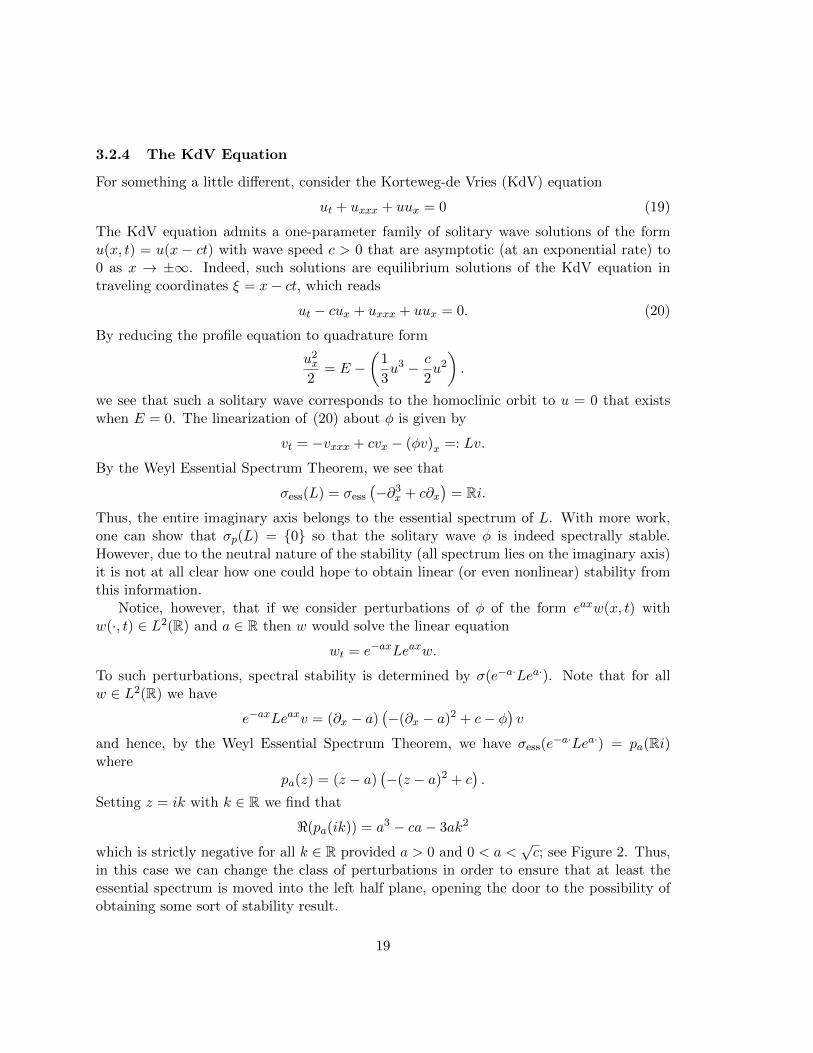
For something a little different, consider the Korteweg-de Vries (KdV) equation
ut + uxxx + uux = 0 (19)
The KdV equation admits a one-parameter family of solitary wave solutions of the formu(x, t) = u(x − ct) with wave speed c > 0 that are asymptotic (at an exponential rate) to0 as x → ±∞. Indeed, such solutions are equilibrium solutions of the KdV equation intraveling coordinates ξ = x− ct, which reads
ut − cux + uxxx + uux = 0. (20)
By reducing the profile equation to quadrature form
u2x
2= E −
(1
3u3 − c
2u2
).
we see that such a solitary wave corresponds to the homoclinic orbit to u = 0 that existswhen E = 0. The linearization of (20) about φ is given by
vt = −vxxx + cvx − (φv)x =: Lv.
By the Weyl Essential Spectrum Theorem, we see that
σess(L) = σess
(−∂3
x + c∂x)
= Ri.
Thus, the entire imaginary axis belongs to the essential spectrum of L. With more work,one can show that σp(L) = {0} so that the solitary wave φ is indeed spectrally stable.However, due to the neutral nature of the stability (all spectrum lies on the imaginary axis)it is not at all clear how one could hope to obtain linear (or even nonlinear) stability fromthis information.
Notice, however, that if we consider perturbations of φ of the form eaxw(x, t) withw(·, t) ∈ L2(R) and a ∈ R then w would solve the linear equation
wt = e−axLeaxw.
To such perturbations, spectral stability is determined by σ(e−a·Lea·). Note that for allw ∈ L2(R) we have
e−axLeaxv = (∂x − a)(−(∂x − a)2 + c− φ
)v
and hence, by the Weyl Essential Spectrum Theorem, we have σess(e−a·Lea·) = pa(Ri)
wherepa(z) = (z − a)
(−(z − a)2 + c
).
Setting z = ik with k ∈ R we find that
<(pa(ik)) = a3 − ca− 3ak2
which is strictly negative for all k ∈ R provided a > 0 and 0 < a <√c; see Figure 2. Thus,
in this case we can change the class of perturbations in order to ensure that at least theessential spectrum is moved into the left half plane, opening the door to the possibility ofobtaining some sort of stability result.
19
(a)
Re(λ )
Im(λ )
-4 -2 2 4
-4
-2
2
4
(b)
Re(λ )
Im(λ )
-4 -2 2 4
-4
-2
2
4
(c)
Re(λ )
Im(λ )
-4 -2 2 4
-4
-2
2
4
Figure 2: For the KdV equation, plots of σess(e−a·Lea·) when c = 1 for (a) a = 0, (b) a = 1
2 ,and (c) a = 1. While the essential spectrum is stable for a ∈ (0, 1), when a > 1 one findsthat the essential spectrum crosses back into the unstable right half plane.
3.3 Linear Stability
We now aim at establishing linear stability from spectral stability information. To begin,we first consider a simpler case where we don’t have essential spectrum to worry about.
To this end, recall that u = 0 is a spectrally stable equilibrium solution of{ut = uxx + u3, t > 0, x ∈ (0, π)
u(0, t) = u(π, t) = 0 ∀t ≥ 0.(21)
In fact, the linearization in this case is given by vt = Lv with L = ∂2x and, moreover, the
eigenvalues are given explicitly by λ−n2, n = 1, 2, 3, . . . with corresponding eigenfunctions
vn(x) = sin(nx). Using the fact that {sin(n·)}∞n=1 forms an orthogonal basis of L2(0, π),it follows from linearity that given any v0 ∈ L2(0, π) the unique solution of the evolutionequation vt = Lv with v ∈ H1
0 (0, π) ∩H2(0, π) and v(x, 0) = v0(x) is given by
v(x, t) =
∞∑n=1
ane−n2t sin(nx)
where an = 2π
∫ π0 v0(x) sin(nx)dx are the Fourier sine coefficients of v0. In particular, we
have from Parseval’s inequality that
‖v(·, t)‖L2(0,π) ≤ e−t‖v0‖L2(0,π),
implying that u = 0 is a linearly stable solution of (21).In the above example, notice we an write v(t) = T (t)v0 where the operator T (t) is given
by
T (t) =
∞∑n=1
2
π〈sin(nx), ·〉L2(0,π) e
−n2t sin(nx).
It is elementary to verify that T (t) is a bounded linear operator on L2(0, π) for all t > 0and that, furthermore, it satisfies
20
(1) T (0) = I, the identify operator.
(2) T (s)T (t) = T (s+ t) = T (t)T (s) for all s, t ≥ 0.
(3) For all v0 ∈ L2(0, π), T (t)v0 → v0 in L2(0, π) as t→ 0+.
Any set of bounded linear operators {T (t)}t≥0 that satisfies (1)-(3) above is called a stronglycontinuous, or C0, semigroup of operators. Notice from the functional properties (1)-(3) itmakes sense to denote
T (t) = eLt t ≥ 0.
Furthermore, in the above example we observed that the fact that <(σ(L)) ≤ −1 impliedthat ∥∥eLtv0
∥∥L2(0,π)
≤ e−t‖v0‖L2(0,π)
so that the decay rate on the linearized solution operator eLt is given exactly by the maxi-mum real part of the spectrum of L.
Not surprisingly, everything said above becomes more difficult when the essential spec-trum is present. For definiteness, let
L = ∂nx + an−1(x)∂n−1x + . . .+ a1(x)∂x + a0(x)
be an nth-order linear differential operator that is densely defined on L2(R) with the co-efficients aj being smooth and exponentially localized functions. In this case, we have thefollowing lemma7.
Lemma 1. Suppose that the exponentially localized operator L above, acting on L2(R), iswell-posed, i.e. there exists an α > 0 such that < (σess(L)) < α. Then L generates a C0
semigroup of operators {T (t)}t≥0 on Hk(R) for every k ≤ n.
The above lemma guarantees that so long as L is well-posed, then for every v0 ∈ L2(R)the unique solution to the linear evolution equation
vt = Lv
with v(0) = v0 is given by v(t) = T (t)v0. As before, due to the fact that T (t) satisfiesproperties (1)-(3) above, we often denote T (t) = eLt. Now, a natural question remainsregarding the connection between the maximum real part of the spectrum of L and thedecay of the linearized semigroup {eLt}t≥0. This is addressed in general by the Gearhart-Pruss Theorem.
Theorem 6 (Gearhart-Pruss). Let X be a Hilbert space and assume L : X → X is a linearoperator with densely defined domain. Let Π be a finite dimensional spectral projection8
associated with L. If there exists constants M,σ > 0 such that∥∥(L− λI)−1(I −Π)f∥∥X≤M‖f‖X ∀f ∈ X (22)
7The forthcoming results come from [KP, Section 4.1].8In particular, one could take Π to be the zero operator.
21
on the set <(λ) ≥ −σ, then there exists a constant C > 0 such that the C0 semigroupassociated with (I −Π)L satisfies the decay estimate∥∥∥e(I−Π)Ltf
∥∥∥X
=∥∥eLt(I −Π)f
∥∥X≤ Ce−σt‖f‖X
for every f ∈ X.
Admittedly, it is often a very difficult task to verify the resolvent operator of L isuniformly bounded on a half space <(λ) > −σ. However, we emphasize that an obviousnecessary condition is <(σ((I − Π)L)) < −σ so that, in particular, it is necessary thatL to be spectrally stable with a spectral gap away from Ri when acting on the invariantsubspace (I − Π)X. Often times, in practice, Π corresponds to projecting out some finitedimensional eigenspace of L. Thankfully, however, there is a commonly occurring class ofoperators where the resolvent bound always holds.
Lemma 2. Suppose the exponentially localized linear operator L above is 2nd-order, andlet Π be a finite dimensional spectral projection for L. Then the uniform resolvent bound(22) holds on <(λ) ≥ −σ + ε for every ε > 0 provided that
<(σ((I −Π)L)) < −σ.
In particular, in this case we are guaranteed that for every ω ∈ (−σ, 0) there exists a constantC = C(ω) > 0 such that ∥∥eLt(I −Π)f
∥∥H1(R)
≤ Ce−ωt‖f‖H1(R)
for every f ∈ H1(R).
In other words, the above lemma guarantees us that if L is a second-order, exponentiallylocalized differential opeartor, then one can obtain decay bounds on the semigroup {eLt}t≥0
directly from the spectral information on L. We will use this observation heavily in ourforthcoming examples. Note that this observation extends to a more general class of so-called “sectorial” operators, where the linearized solution operator can be defined via theholomorphic functional calculus as
eLt =1
2πi
∫Γ
eλt
λI − Ldλ,
where here Γ is some curve in C going from α− i∞ to α + i∞ for some α > max<(σ(L))that is always to the right of the spectrum of L. While there is some serious fun one canhave here trying to obtain properties of eLt through the use of complex analytic techniques,we leave this as an exercise for the interested reader.
22
3.4 Linear Stability of Monotone Front
Consider again the reaction diffusion equation
ut = uxx + u− u3, x ∈ R, t > 0 (23)
and recall above we verified that (23) admits a stationary front solution φ that is strictlymonotone and satisfies
limx→−∞
φ(x) = −1, limx→+∞
φ(x) = 1.
Furthermore, recall that we have already established the following spectral properties ofL = ∂2
x + 1 − 3φ2, considered here as an operator on L2(R) with densely defined domainH1(R):
1. The essential spectrum is given explicitly by σess(L) = (−∞,−2].
2. 0 ∈ σp(L) with eigenfunction φ′.
3. There exists a γ > 0 such that σp(R) \ {0} < −γ.
Defining Π : L2(R)→ ker(L) to be the spectral projection
Π :=〈φ′, ·〉L2
‖φ′‖2L2
φ′
and noting that σ(ΠL) < −γ, it follows from the work in the previous section that Lgenerates a C0 semigroup {eLt}t≥0 and, furthermore, that for every ω ∈ (0, γ) there existsa constant C = C(ω) > 0 such that∥∥∥e(I−Π)Ltv(0)
∥∥∥L2
. e−ωt‖v(0)‖L2
for all t ≥ 0.Since we had to project out the kernel of L to establish the above linear decay result,
we can not conclude linear stability of φ from here. Indeed, it is a-priori possible thatinitially nearby solution u(t) simply “drifts” along the center manifold associated withKer(L). Nevertheless, in this case we can show the following linear, asymptotic orbitalstability result:
‖v(t)−Π(v(0))‖L2 ≤ Ce−ωt‖v(0)‖L2 .
In particular, this motivates that v(t) will converge to some multiple, depending on v(0),of φ′ as t → ∞, i.e. for given initial data, to a fixed element of the “center subspace”. Interms of the original solution u(x, t), this suggests that an initially nearby solution u(x, 0)will satisfy
u(x, t) ≈ φ(x) + v(x, t)
≈ φ(x) + γ∞φ′(x) for t� 1
≈ φ (x+ γ∞)
23
if ‖v(0)‖H1 � 1, where here γ∞ =〈ψ′,v(0)〉L2
‖φ′‖2L2
and the last approximation follows by Taylor’s
theorem. This implies that one should expect that a solution that starts near the stationaryfront φ will evolve into a slight spatial translate of φ. In a later section, we will verify thisbehavior at the nonlinear level.
3.5 The Periodic Case
Recall that if L is a linear operator of the form (5) with T -periodic coefficients, consideredhere as acting on L2(R), then
σ(L) = σess(L) =⋃
ξ∈[−π/T,π/T )
σL2per(0,T )(Lξ)
where here Lξ := e−iξxLeiξx are the Bloch operators. A natural question arises in howT -periodic spectral information about the Bloch operators Lξ influence the behavior of thelinearized smigroup eLt. This is most easily seen through the introduction of the Bloch, orFloquet-Bloch, transform.
To motivate this, notice that given any v ∈ L2(R) we can express v in terms of itsinverse Bloch representation as
v(x) =
∫ T/2
−T/2eiξTxv(ξ, x)dξ
where here v(ξ, x) :=∑
k∈Z eikTxv(ξ + kT ) are T -periodic functions of x, where here v
denotes the Fourier transform of v. Indeed, the above formulas may be easily checked onthe Schwartz class by grouping frequencies that differ by T in the standard Fourier transformrepresentation of v:
v(x) =∑k∈Z
∫ T/2
−T/2ei(ξ+kT )xv(ξ + kT )dξ =
∫ T/2
−T/2eiξxv(ξ, x)dξ.
The Bloch transform
B : L2(R)→ L2([−T/2, T/2);L2per(0, T ))
given by B(v)(ξ, x) := v(ξ, x) is then well-defined, bijective and continuous. In fact, for agiven v ∈ L2(R) one can show that B(Lv)(ξ, x) = Lξ[v(ξ, ·)](x), and hence that the Blochoperators Lξ may be viewed as operator-valued symbols under B, acting on L2
per(0, T ).
Similarly, from the identity B(eLtv
)=(eLξtv(ξ, ·)
)(x), we find the Bloch solution formula
for the periodic-coefficient operator L:
(eLtv
)(x) =
∫ π/T
−π/Teiξx
(eLξtv(ξ, ·)
)(x)dξ. (24)
24
It follows that the Bloch transform B diagonalizes the periodic coefficient operators L inthe same way that the Fourier transform diagonalizes constant-coefficient operators.
Using the representation formula (24), bounds on the Bloch solution operators eLξt,which are governed by the the T -periodic eigenvalues of the Bloch operators Lξ, can beconverted to bounds on the linearized solution operator eLt. Indeed, using the classicalParseval theorem we note that for all v ∈ L2(R) that
‖v‖2L2(R) = 2π
∫ T/2
−T/2
∫ T
0|B(v)(ξ, x)|2 dz dξ
so that the rescaled Bloch transform√
2πB is an isometry from L2(R) into the spaceL2([−T/2, T/2);L2
per(0, T )). More generally, by interpolating with the triangle inequal-ity, corresponding to (p, q) = (∞, 1) below, we obtain the generalized Hausdorff-Younginequality
‖v‖Lp(R) ≤ Cp,q ‖B(v)‖Lq([−π/T,π/T );Lpper(0,T )
for q ≤ 2 ≤ p and 1p + 1
q = 1. This immediately gives us the result∥∥eLtv∥∥Lp(R)
≤ Cp,q∥∥eLξtv(ξ, ·)
∥∥Lqξ([−π/T,π/T );Lpper(0,T ))
(25)
which allows one to obtain estimates on the linearized semigroup eLt from estimates on theBloch semigroups eLξt.
4 Nonlinear Stability: Examples
In this section, we present a few examples where the above theories can be applied to yieldnonlinear stability of solutions of PDE’s. In the first example, we will see an example wherethe linearized operator about the trivial solution admits a spectral gap, and will establishthat this trivial solution is in fact asymptotically stable In the second example, we studythe case when the spectrum of the linearized operator is stable with a spectral gap, exceptfor the existence of a simple eigenvalue at the origin coming from the translation invarianceof the PDE. Finally, we will discuss complications that arise when considering the stabilityof periodic patterns to localized (i.e. integrable on R) perturbations, and how the ideaspresented in these notes can be used to study the nonlinear stability of such patterns.
4.1 Reaction Diffusion on Bounded Domain
Consider the PDEut = uxx + u3, t > 0, x ∈ (0, π) (26)
equipped with the homogeneous Dirichlet boundary conditions
u(0, t) = u(π, t) = 0 ∀t ≥ 0.
25
We consider the above as an evolution equation on L2(0, π). Clearly u = 0 is an equilibriumsolution of (26), and here we are interested in the stability of this so-called “trivial solution”.To this end, we consider the above PDE with the initial condition
u(x, 0) = 0 + v0(x)
where ‖v0‖H1(0,π) � 1 and v0(0) = v0(π) = 0, and note there exists a unique solution v(t)of (26) defined locally in time and v(t) satisfies v(0, t) = v(π, t) = 0 for so long as v(t) isdefined. Defining the operator L := ∂2
x and the nonlinear operator N(v) = v3, we note v(t)solves the evolution equation
vt = Lv +N(v) (27)
Here, we consider L as being densely defined on L2(0, π) with domain D(L) := H10 (0, π) ∩
H2(0, π). Recall from previous work that we have <(σ(L)) ≤ −1 and that the associatedlinearized semigroup {eLt}t≥0 obeys the exponential decay bound∥∥eLtf∥∥
H1(0,π)≤ Ce−t ‖f‖H1(0,π) ∀f ∈ D(L)
valid for some constant C > 0.To establish the nonlinear stability of u = 0, we note that we can rewrite the nonlinear
perturbation equation (27) as the equivalent integral equation
v(t) = eLtv(0) +
∫ t
0eL(t−s)N(v(s))ds,
which, as it is for ODE, is sometimes called “Duhamel’s formula”. Our goal is to prove thatu = 0 is nonlinearly stable in the following sense.
Theorem 7. For each ω ∈ (−1, 0), there exists a δ, C = C(ω, δ) > 0 such that if u0 ∈ D(L)with
‖u0‖H1(0,π) < δ
then the unique solution u(t) of (26) with u(0) = u0 satisfies
‖u(t)‖H1(0,π) ≤ Ce−ωt‖u0‖H1(0,π).
for all t ≥ 0.
Remark 7. This is purely a local stability result. Indeed, one can show that if ‖u0‖H1(0,π)
is too large, then the solution u(t) of the IVBVP (26) blows up in finite time. Specifically,one can show that if
S(t) :=1
π
∫ π
0u(x, t) sin(x)dx
denotes the first Fourier sine coefficient of the solution u(t), then S satisfies the differentialinequality
S′(t) ≥ −S(t) +π2
4S(t)3
26
which, thanks to Gronwall’s inequality, implies there exists a finite t∗ > 0 such that S(t)→+∞ as t→ t−∗ . It follows that ‖u(t)‖H1(0,π) must blow up at least by time t∗. Note it couldblow up before time t∗ if a higher order Fourier coefficient blows up first. Regardless, thisemphasizes the fact that stability is a purely local theory.
To prove this theorem, we start by noting that, thanks to the Sobolev embeddingL∞(0, π) ⊂ H1(0, π), the nonlinear term N(v) is well defined in H1 and satisfies
‖N(u)‖H1(0,π) ≤M‖u‖3H1(0,π)
for some constant M > 0 independent of u; indeed, recall that Hs(0, π) is an algebra whens > 1
2 . Furthermore, by the local well posedness, given any R > 0 sufficiently small andu0 ∈ H1(0, π) with ‖u0‖H1(0,π) <
R2 then there exists a T = T (u0) > 0 such that the
(26) with initial condition u(0) = u0 has a unique solution u(t) ∈ H1(0, π) defined for allt ∈ [0, T ) such that
‖u(t)‖H1(0,π) < R ∀t ∈ [0, T ).
By the exponential decay bound on eLt and the triangle inequality, we find from Duhamel’sformula that
‖u(t)‖H1(0,π) ≤ Ce−t‖u(0)‖H1(0,π) + C
∫ t
0e−(t−s) ‖N(u(s))‖H1(0,π) ds
≤ Ce−t‖u(0)‖H1(0,π) + CM
∫ t
0e−(t−s)‖u(s)‖3H1(0,π)ds.
The above integral inequality implies the desired decay bound. We will establish this usingtwo separate arguments: the first via a more classical ODE approach using Gronwall’sinequality, and the second using a different approach that will be more suitable to ourforthcoming PDE applications.
For our first proof of the above claim, observe that since ‖u(t)‖H1(0,π) < R for allt ∈ [0, T ) we have
et‖u(t)‖H1(0,π) ≤ C‖u(0)‖H1(0,π) + CMR2
∫ t
0es‖u(s)‖H1(0,π).
Gronwall’s inequality now immediately gives that
et‖u(t)‖H1(0,π) ≤ C‖u(0)‖H1(0,π)eCMR2t
for all t ∈ [0, T ). Choosing R > 0 sufficiently small that ω := 1− CMR2 > 0 and choosingε ∈ (0, R2 ) such that Cε < R
4 it follows that if ‖u(0)‖H1(0,π) < ε then
‖u(t)‖H1(0,π) ≤ C‖u(0)‖H1(0,π)e−ωt ∀t ∈ [0, T )
and, further, that ‖u(t)‖H1(0,π) <R2 for all t ∈ [0, T ). By extensibility, it follows that
T = +∞ and the above bounds hold for all t ≥ 0, as claimed. We note that while the
27
above “Gronwall” argument works very well in this case, it is not suitable for our intendedapplications to problems on the whole line.
As an alternative for the above Gronwall based argument, for all t ∈ [0, T ), define thequantity
Z(t) := sup0≤s≤t
es‖u(s)‖H1(0,π)
and note the expected decay rate follows from showing that Z is uniformly bounded. Now,for all t ∈ [0, T ) and s ∈ [0, t] we have
‖u(s)‖H1(0,π) = e−s(es‖u(s)‖H1(0,π)
)≤ e−sZ(t)
so that, if we fix t ∈ [0, T ) we have for all t′ ∈ [0, t)
‖u(t′)‖H1(0,π) ≤ Ce−t′‖u(0)‖H1(0,π) +M
∫ t′
0e−(t′−s)e−3sZ(s)3ds
and hence
et′‖u(t′)‖H1(0,π) ≤ C‖u(0)‖H1(0,π) + CM
(∫ t′
0e−2sds
)Z(t)3
≤ C‖u(0)‖H1(0,π) + MZ(t)3
where here M = CM . Taking the supremium in t′ ∈ [0, t) it follows that
Z(t) ≤ C‖u(0)‖H1(0,π) + MZ(t)3.
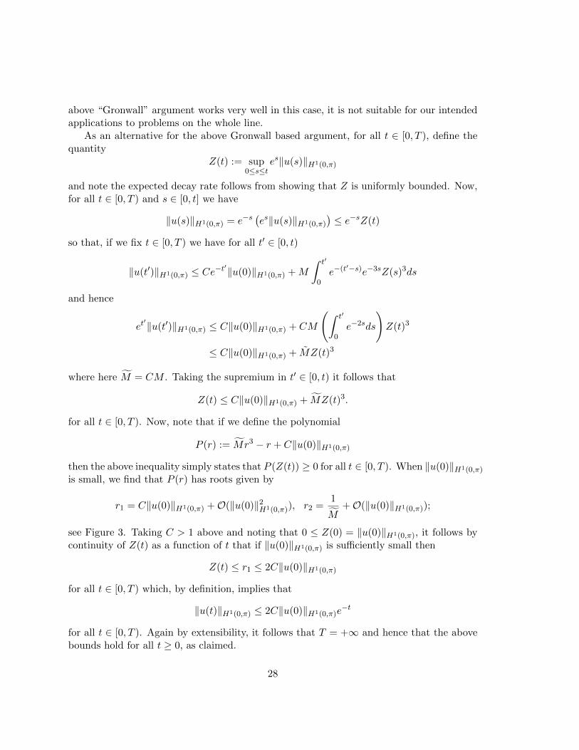
for all t ∈ [0, T ). Now, note that if we define the polynomial
P (r) := Mr3 − r + C‖u(0)‖H1(0,π)
then the above inequality simply states that P (Z(t)) ≥ 0 for all t ∈ [0, T ). When ‖u(0)‖H1(0,π)
is small, we find that P (r) has roots given by
r1 = C‖u(0)‖H1(0,π) +O(‖u(0)‖2H1(0,π)), r2 =1
M+O(‖u(0)‖H1(0,π));
see Figure 3. Taking C > 1 above and noting that 0 ≤ Z(0) = ‖u(0)‖H1(0,π), it follows bycontinuity of Z(t) as a function of t that if ‖u(0)‖H1(0,π) is sufficiently small then
Z(t) ≤ r1 ≤ 2C‖u(0)‖H1(0,π)
for all t ∈ [0, T ) which, by definition, implies that
‖u(t)‖H1(0,π) ≤ 2C‖u(0)‖H1(0,π)e−t
for all t ∈ [0, T ). Again by extensibility, it follows that T = +∞ and hence that the abovebounds hold for all t ≥ 0, as claimed.
28
r
P(r)
|| u(0) ||H^1
r1 r20
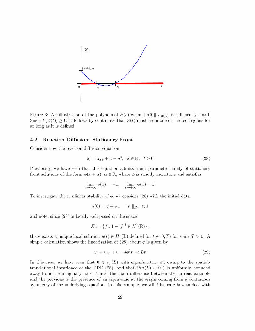
Figure 3: An illustration of the polynomial P (r) when ‖u(0)‖H1(0,π) is sufficiently small.Since P (Z(t)) ≥ 0, it follows by continuity that Z(t) must lie in one of the red regions forso long as it is defined.
4.2 Reaction Diffusion: Stationary Front
Consider now the reaction diffusion equation
ut = uxx + u− u3, x ∈ R, t > 0 (28)
Previously, we have seen that this equation admits a one-parameter family of stationaryfront solutions of the form φ(x+ α), α ∈ R, where φ is strictly monotone and satisfies
limx→−∞
φ(x) = −1, limx→+∞
φ(x) = 1.
To investigate the nonlinear stability of φ, we consider (28) with the initial data
u(0) = φ+ v0, ‖v0‖H1 � 1
and note, since (28) is locally well posed on the space
X :={f : 1− |f |2 ∈ H1(R)
},
there exists a unique local solution u(t) ∈ H1(R) defined for t ∈ [0, T ) for some T > 0. Asimple calculation shows the linearization of (28) about φ is given by
vt = vxx + v − 3φ2v =: Lv (29)
In this case, we have seen that 0 ∈ σp(L) with eigenfunction φ′, owing to the spatial-translational invariance of the PDE (28), and that <(σ(L) \ {0}) is uniformly boundedaway from the imaginary axis. Thus, the main difference between the current exampleand the previous is the presence of an eigenvalue at the origin coming from a continuoussymmetry of the underlying equation. In this example, we will illustrate how to deal with
29
this additional complication through the introduction of a “modulation function” that, insome sense, will ensure the nonlinear perturbation always lies in the stable subspace of thelinearized operator L.
Recall, through a detailed study of σ(L) and the resulting bounds on the linearizedsemigroup {eLt}t≥0, we have seen that by defining Π : L2(R) → ker(L) to be the spectralprojection
Π :=〈φ′, ·〉L2
‖φ′‖2L2
φ′
the linearized semigroup {eLt}t≥0 satisfies the decay estimate: for every ω ∈ (0, γ) thereexists a constant C = C(ω) > 0 such that∥∥eLt(I − P )v(0)
∥∥L2 . e−ωt‖v(0)‖L2
for all t ≥ 0. In particular, we demonstrated that this gives the following linear, asymptoticorbital stability result:
‖v(t)−Π(v(0))‖L2 ≤ Ce−ωt‖v(0)‖L2 .
Of particular importance, this leads us to suspect that v(t) will converge to a multiple,depending on v(0), of φ′ as t → ∞, i.e. for given initial data, to a fixed element of the“center subspace”. In terms of the original solution u(x, t), this suggests that an initiallynearby solution u(x, 0) will satisfy
u(x, t) ≈ φ (x+ γ∞) for t� 1,
where here γ∞ =〈ψ′,v(0)〉L2
‖φ′‖2L2
. This implies that one should expect that a solution that starts
near the stationary front φ will evolve into a slight spatial translate of φ.To verify the above prediction at a nonlinear level, first notice in the “classical” notion
of asymptotic stability, one aims at showing u(t) → φ as t → ∞ and hence we want tocontrol the distance from u(t) to φ. This motivates introducing the perturbation variable
v(t) = u(t)− φ
defined for t ∈ [0, T ). However, here we expect that u(t) → φ(· + γ∞) as t → ∞ for someγ∞ small. Consequently, in this case we want to control the distance from u(t) to the1-dimensional manifold
M := {φ(·+ γ) : γ ∈ R} ⊂ H1(R). (30)
This motivates the introduction of the new perturbation variable
v(t) = u(t)− φ(· − γ(t)), t ∈ [0, T )
where γ(t) is some function to be determined. The function γ(t) is sometimes called a“modulation function”. Note that regardless of how γ(t) is chosen above, for all t ∈ [0, T )we have
and so we are free to choose γ(t) above to fit our needs.Motivated by above, we begin by determining a suitable foliation for a small “tubular”
neighborhood of the manifold M in H1(R), i.e. a local coordinate system defined in aneighborhood of the orbit of φ that is suitable for our needs. This can be done in anumber of ways, and one will find many different such foliations in the literature. Since thelinearized semigroup eLt is exponentially stable when restricted to Ker(L)⊥, here we wouldlike to choose γ(t) such that v ∈ Ker(L)⊥ for all t ∈ [0, T ).
Lemma 3. There exists a δ > 0 and smooth functions (γ, v) : H1(R) → R ×H1(R) withγ(φ) = 0, v(M) = 0 such that if u ∈ H1(R) with
dist(u,M) := infz∈R‖u− φ(·+ z)‖H1 < δ,
thenu = φ(·+ γ(u)) + v(u)
where v(u) ∈ Ker(L)⊥.
Proof. Suppose, without loss of generality, ‖u − φ‖H1 is small. For each such u, want toshow there exists a γ ∈ R with γ(φ) = 0 such that⟨
φ′, u− φ(·+ γ)⟩H1︸ ︷︷ ︸
g(γ,u)
= 0.
Since g is smooth with g(0, φ) = 0 and ∂γ(0, φ) = −‖φ′‖2L2 6= 0, the result follows by theimplicit function theorem.
Thus, if ‖u− φ‖H1 < δ2 and
v(t) := u(t)− φ(·+ γ(t))
then by possibly choosing T > 0 smaller above we can assume γ(t) is such that
v(t) ∈ Ker(L)⊥ ∀ t ∈ [0, T )
and, further, without loss of generality that γ(0) = 0 (else, can consider the stability of atranslate of φ.
Now, since u(t) solves (28) for all t ∈ [0, T ), it follows that the functions v(t) and γ(t)satisfy
∂t (v + φ(·+ γ(t))) = ∂2x (v(t) + φ(·+ γ(t))) + (v + φ(·+ γ(t)))− (v + φ(·+ γ(t)))3
for all t ∈ [0, t) which, using that φ(·+γ(t)) is a stationary solution of (28), can be rewrittenas
vt + φ′(·+ γ(t))γ′(t) = Lγ(t)v +Nγ(t)(v) (31)
31
where hereLγ(t) = ∂2
x + 1− 3φ(·+ γ(t))2
denotes the linearization of (28) about the translate φ(·+ γ(t)) and
Nγ(t)(v) = −3v2φ(·+ γ(t))− v3
is a nonlinear functional. Now, we can not apply our semigroup theory and estimates to(31) since the coefficients of the linear operator Lγ(t) depend on the evolution variable t.To compensate for this, we simply observe that
Lγ(t) = L+[Lγ(t) − L
]and hence treat the operator Lγ(t) − L as an additional nonlinearity. It follows that v(t)and γ(t) satisfy the equation
Next, we decompose (32) according to the orthogonal decomposition H1 = Ker(L) ⊕Ker(L)⊥. Applying the spectral projection Π to (32) gives
Π(vt) + Π(φ′(·+ γ(t))φ′(t)
)= ΠLv + ΠR(γ(t), v).
Since Π(v) = 0 for all t ∈ [0, T ) we have Π(vt) = ∂tΠ(v) = 0. Furthermore, since Π is aspectral projection for L, the operators L and Π commute and hence Π ◦ L = L ◦ Π = 0.We may thus rewrite the above equation as⟨
φ′, φ′(·+ γ(t))⟩γ′(t) =
⟨φ′,R(γ(t), v)
⟩From here, we an derive estimates on γ′ as follows. Note that
⟨φ′, φ′(·+ γ(t))
⟩=⟨φ′, φ′
⟩+
⟨φ′, φ′(·+ γ(t))− φ′︸ ︷︷ ︸
z(t)
⟩
Since ‖z(t)‖ ≤ ‖φ′′‖|γ(t)|, it follows that so long as γ(t) is small, say for all t ∈ [0, T ) withT > 0 possibly smaller than before, the above says
|γ′(t)| ≤ C(1 + γ(t))∣∣⟨φ′,R(γ(t), v)
⟩∣∣for all t ∈ [0, T ) for some constant C > 0. Similarly, noting that
‖R(γ(t), v)‖ ≤ C(‖v‖2 + |γ(t)|‖v‖
)it follows that, by possibly choosing T > 0 smaller yet again (so that ‖v‖H1 is sufficientlysmall for all t ∈ [0, T )),
|γ′(t)| ≤ C(‖v(t)‖2H1 + |γ(t)|‖v(t)‖
)32
for all t ∈ [0, T ).Next, we project (32) onto the stable subspace Ker(L)⊥. Applying (I − Π) to (32) we
getvt + (I −Π)φ′(·+ γ(t))γ′(t) = Lv + (I −Π)R(γ(t), v).
As above, we can rewrite the second term as
(I −Π)[(φ′ + (φ′(·+ γ(t))− φ′)
)γ′(t)
]= (I −Π)z(t)γ′(t)
so thatvt = Lv + (I −Π)
[R(γ(t), v)− z(t)γ′(t)
].
Setting RF (γ(t), v) := R(γ(t), v) − z(t)γ′(t), it follows that for all t ∈ (0, T ) the functionsγ(t) and v(t) satisfy the coupled system
γ′(t) = O(‖v(t)‖2H1 + |γ(t)|‖v(t)‖H1
)v(t) = eLtv(0) +
∫ t
0eL(t−s) (I −Π)RF (γ(s), v(s))ds.
(33)
Now, we know that if ω ∈ (0, γ) then there exists a C = C(ω) > 0 such that∥∥eLtf∥∥H1 ≤ Ce−ωt‖f‖H1 ∀ f ∈ Ker(L)⊥.
Fix such an ω and fix ω ∈ (ω/2, ω) and define for all t ∈ [0, T ) the functions
Mv(t) := sup0≤s≤t
eωs‖v(s)‖H1 , Mγ(t) := sup0≤s≤t
|γ(s)|.
Note that for all t ∈ [0, T ) and s ∈ [0, t] we have
‖v(s)‖H1 ≤ e−ωsMv(t), |γ(s)| ≤Mγ(t).
Our goal is to show that Mv and Mγ are uniformly bounded in time.To this end, notice that if we fix t ∈ [0, T ) and integrate (33)(i) from [0, t′] for some
t′ ∈ [0, t] we have
γ(t′)− γ(0) =
∫ t′
0O(‖v(s)‖2H1 + |γ(s)|‖v(s)‖H1
)ds.
Since γ(0) = 0 by choice, it follows that
|γ(t′)| ≤ C
[(∫ t′
0e−2ωsds
)Mv(t)
2 +
(∫ t′
0e−ωs
)Mγ(t)Mv(t)
]for some constant C > 0. Noting that the scalar integrals above are uniformly bounded int′, taking the supremium over t′ ∈ [0, t] implies there exists a constant C1 > 0 such that
Mγ(t) ≤ C1
(Mv(t)
2 +Mγ(t)Mv(t))
33
for all t ∈ [0, T ). Similarly, for 0 ≤ t′ ≤ t < T as above, from (33)(ii) we get
‖v(t′)‖H1 ≤ Ce−ωt′ ‖v(0)‖H1 + C
∫ t′
0e−ω(t′−s) ‖(I −Π)RF (γ(s), v(s))‖H1 ds.
Since (I −Π) is clearly a bounded linear operator on H1, we have by the above work that
Noting that the exponentials on the right hand side above are uniformly bounded above int′, we find by taking the supremum in t′ ∈ [0, t] that there exists a constant C2 > 0 suchthat
Mv(t) ≤ C2
(‖v(0)‖H1 +Mv(t)
2 +Mγ(t)Mv(t)).
Next, we claim that if ‖v(0)‖H1 and T > 0 are such that
Mv(t) ≤1
2C1∀t ∈ [0, T )
then T = +∞ and, in particular, Mv(t) is well defined and uniformly bounded for all t ≥ 0.To see this, note that by the above condition on T we have
Mγ(t) ≤ 1
2Mγ(t) + C1Mv(t)
2
and hence thatMγ(t) ≤ 2C1Mv(t)
2 ∀t ∈ [0, T ).
34
Inserting this into the bound for Mv(t) gives
Mv(t) ≤ C(‖v(0)‖H1 +Mv(t)
2 +Mv(t)3)∀t ∈ [0, T ).
where C > 0 is some constant. Now, define the polynomial
P (r) = r3 + r2 − 1
Cr + ‖v(0)‖H1
and note the above inequality states that P (Mv(t)) ≥ 0 for all t ∈ [0, T ). One can easilycheck that for ‖v(0)‖H1 sufficiently small, P (r) has two consecutive positive roots r1, r2
satisfying0 < r1 = C‖v(0)‖H1 +O(‖v(0)‖2H1)� r2
with P (r) ≥ 0 for r ∈ [0, r1] ∪ [r2,∞) and P (r) < 0 for r ∈ (r1, r2). Taking C > 1 above, itfollows that
Mv(0) = ‖v(0)‖H1 < r1
so that, by continuity of Mv(t) on t, we have
Mv(t) ≤ r1 ≤ 2C‖v(0)‖H1
for all t ∈ [0, T ), provided that ‖v(0)‖H1 is sufficiently small. In particular, if we choose‖v(0)‖H1 sufficiently small that r1 <
12C1
then the above argument can be continued to giveT = +∞. We conclude that if ‖v(0)‖H1 is sufficiently small, then there exists a constantC > 0 such that Mv(t) ≤ C‖v(0)‖H1 for all t ≥ 0 so that, in particular,
‖v(t)‖H1 ≤ Ce−ωt‖v(0)‖H1 ∀t ≥ 0.
This verifies that the perturbed solution u(t) converges as t→∞ to the one-dimensionalmanifold M. To show that it converges to a particular element of M, recall that for allt ≥ 0 we have
γ′(t) = O(‖v(t)‖2H1 + |γ(t)|‖v(t)‖H1
)and that |γ(t)| ≤Mγ(t) ≤ 2C1Mv(t)
2. By the above bound on Mv(t) it follows that
γ′(t) = O(e−2ωt‖v(0)‖2H1 + e−ωt‖v(0)‖3H1
).
Fixing 0 ≤ t1 < t2 and integrating over [t1, t2], it follows there exists a constant C > 0 suchthat
|γ(t2)− γ(t1)| ≤ C∫ t2
t1
(e−2ωt‖v(0)‖2H1 + e−ωt‖v(0)‖3H1
)dt
≤ C(
1
2ωe−2ωt1‖v(0)‖2H1 +
1
ωe−ωt1‖v(0)‖3H1
)≤ Ce−ωt1‖v(0)‖2H1
35
provided that ‖v(0)‖H1 is sufficiently small. It follows that the sequence {γ(t)}t≥0 is aCauchy sequence in R and hence there exists a γ∞ ∈ R such that
γ(t)→ γ∞ as t→∞.
In particular, the above bound gives
|γ(t)− γ∞| ≤ Ce−ωt‖v(0)‖2H1
so that γ(t) converges to γ∞ at an exponential rate.Putting everything together, we have shown that the perturbed solution u(t) converges
to φ(·+ γ∞) ∈M at an exponential rate as t→∞, as claimed.
4.3 Discussion of the Periodic Case
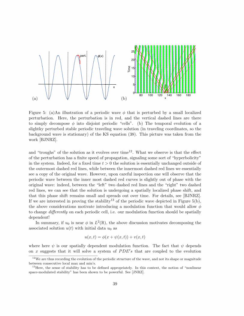
Finally, let’s briefly discuss how the previous techniques might be applied in the periodicsetting. To this end, consider a PDE of the form
ut = F (u) (34)
where we assume F is a constant coefficient (in both x and t) nonlinear operator, andsuppose that (34) has a T -periodic equilibrium solution φ(x). For this discussion, we areinterested in determining the stability of φ to so-called “localized” perturbations9, i.e. toperturbations in L2(R). The linearized operator, obtained by linearizing the right hand sideof (34) about φ is the operator
L := DF (φ)
which will be a linear differential operator with T -periodic coefficients. From our previouswork, we know the spectrum of L can be decomposed as
σL2(R)(L) =⋃
ξ∈[−π/T,π/T )
σL2per(0,T )(Lξ),
where the Bloch operators Lξ := e−iξxLeiξx are considered to act on L2per(0, T ) for each
ξ ∈ [−π/T, π/T ). By Remark 6 in Section 3.2.3 above, it follows that φ′ satisfies the ODE
Lφ′ = 0. (35)
Unlined the analysis in Section 3.2.2 and Section 3.2.3, this does not imply that λ = 0 isan eigenvalue10 of L since φ′, being T -periodic, clearly does not belong to L2(R). Rather,(35) implies that λ = 0 is an eigenvalue for the co-periodic Bloch operator L0.
For the sake of simplicity, assume that λ = 0 is a simple eigenvalue of L0, and that0 /∈ σp(Lξ) for any ξ 6= 0. Then as ξ is varied near ξ = 0, there exists a curve of essential
9Note if one wishes to study the stability of φ to periodic perturbations, as discussed in Section 2.3.1,then σp(L) is purely discrete and stability may be studied in much the same way as in the above examples.
10And, recall that we already know that σp(L) = ∅ anyways.
36
Re(λ)
Im(λ)
0
λ(ξ)
Figure 4: An illustration of the spectrum about a stable periodic equilibrium solution of(34) near the origin λ = 0.
spectrum λ(ξ) ∈ σp(Lξ) near the origin which, by basic results in spectral perturbationtheory, is analytic in ξ and satisfies
λ(ξ) = λ(−ξ)
for all |ξ| � 1. It follows that if φ is to be a stable equilibrium solution of (34), then λ(ξ)must admit a Taylor expansion for |ξ| � 1 of the form
λ(ξ) = iαξ − βξ2 +O(|ξ|3)
for some constants α ∈ R and β ≥ 0. If we assume the non-degeneracy condition β 6= 0, itfollows that11
<(σp(Lξ)) ≤ −θξ2 ∀0 < |ξ| � 1. (36)
Considering now the linear stability of φ, let ε0 > 0 be small and recall the Bloch solutionformula(
eLtv)
(x) =
∫|ξ|<ε0
eiξx(eLξtv(ξ, ·)
)(x)dξ +
∫ε0<|ξ|< π
T
eiξx(eLξtv(ξ, ·)
)(x)dξ, (37)
where here we have separated the low- and high-Bloch number components of the integral.If we assume that there exists a constant σ > 0 such that
<(σp(Lξ)) < −σ for all ε0 < |ξ| <π
T,
it follows by the generalized Hausdorff-Young (25) inequality that∥∥∥∥∥∫ε0<|ξ|< π
11Concerning modeling, such a condition may be expected to hold for stable waves in diffusive, either fullyor partially, systems. In energy conserving Hamiltonian systems (such as the KdV equation (19)), rather,spectral stability is equivalent to σ(L) ⊂ Ri. In such a case, it is not yet known how to establish nonlinearstability through the method of linearization, and one typically relies on different methods, such as the studyof an appropriate Lyapunov functional.
37
so that the second term in (37) decays exponentially fast in time. On the other hand, thefirst term in (37) satisfies∥∥∥∥∥
∫|ξ|<ε0
eiξx(eLξtv(ξ, ·)
)(x)dξ
∥∥∥∥∥L2x(R)
C ≤∥∥∥e−θξ2tv(ξ, x)
∥∥∥L2([−π/T,π/T );L2(0,T )
≤∥∥∥e−θξ2t∥∥∥
L∞ξ
‖v‖L2([−π/T,π/T );L2(0,T )
≤ C‖v‖L2(R)
Consequently, these calculations show the first term in (37) is only bounded in time, andhence does not decay.
Remark 8. It is actually possible to sharpen the above estimate to yield a t−1/4 decay rate,but this ends up being too slow to close any reasonable iteration scheme that might lead toa nonlinear stability result.
So then, how might one go about establishing a nonlinear stability result in this case?In a sense, we should follow the ideas in Section 4.2 and introduce an appropriate “modu-lation” function to accommodate for the lack of decay. As expected, however, this is morecomplicated in this case. To see why, observe that in Section 4.2 that a spatially uniformtranslation of the front still satisfies the same boundary conditions as the front. In particu-lar, the Lp(R) norm between any two elements of the manifold M in (30) is finite. For ourT -periodic equilibrium solution of (34), however, periodicity implies that for any γ 6= ZTthat
‖φ− φ(·+ γ)‖Lp(R) = +∞ for all 1 ≤ p <∞
In other words, a spatially uniform translation of a periodic wave is not a small, or evenbounded, perturbation in Lp(R) for any finite 1 ≤ p <∞.
To proceed, let’s think about the expected dynamics about a “stable” periodic wave φ.Suppose φ is as in Figure 5(a), and note that we can decompose x-axis into periodic “cells”corresponding to the periodicity of φ. If we perturb φ by a small localized perturbationas in Figure 5(a), it is natural to expect that it effect of this perturbation has a finitespeed of propagation. In particular, at any given time each periodic cell may react tothe initial perturbation differently. To further illustrate this point, it is known that thereexists “spectrally stable” periodic traveling wave solutions to the Kuramoto-Sivashinsky(KS) equation
ut + uxxx + uux + δ(uxx + uxxxx) = 0. (38)
While we won’t go into the details of the analysis or proof, which can be found in [BJNRZ],it is instructive to view the dynamics of such a stable solution: see Figure 5(b). In thisfigure, start at t = 0 with a stable periodic traveling wave solution of (38) and perturb itby some small, localized “bump” around x = 130. The effect of the perturbation on thesolution tracked as time is increased: here, the green and blue curves denote the “peaks”
38
(a)
x
ϕ(x)pert.
(b)80 100 120 140 160 180
0
5
10
15
20
25
x
Tim
e
Figure 5: (a)An illustration of a periodic wave φ that is perturbed by a small localizedperturbation. Here, the perturbation is in red, and the vertical dashed lines are thereto simply decompose φ into disjoint periodic “cells”. (b) The temporal evolution of aslightky perturbed stable periodic traveling wave solution (in traveling coordinates, so thebackground wave is stationary) of the KS equation (38). This picture was taken from thework [BJNRZ].
and “troughs” of the solution as it evolves over time12. What we observe is that the effectof the perturbation has a finite speed of propagation, signaling some sort of “hyperbolicity”in the system. Indeed, for a fixed time t > 0 the solution is essentially unchanged outside ofthe outermost dashed red lines, while between the innermost dashed red lines we essentiallysee a copy of the original wave. However, upon careful inspection one will observe that theperiodic wave between the inner most dashed red curves is slightly out of phase with theoriginal wave: indeed, between the “left” two dashed red lines and the “right” two dashedred lines, we can see that the solution is undergoing a spatially localized phase shift, andthat this phase shift remains small and spreads out over time. For details, see [BJNRZ].If we are interested in proving the stability13 of the periodic wave depicted in Figure 5(b),the above considerations motivate introducing a modulation function that would allow φto change differently on each periodic cell, i.e. our modulation function should be spatiallydependent!
In summary, if u0 is near φ in L2(R), the above discussion motivates decomposing theassociated solution u(t) with initial data u0 as
u(x, t) = φ(x+ ψ(x, t)) + v(x, t)
where here ψ is our spatially dependent modulation function. The fact that ψ dependson x suggests that it will solve a system of PDE′s that are coupled to the evolution
12We are thus recording the evolution of the periodic structure of the wave, and not its shape or magnitudebetween consecutive local max and min’s.
13Here, the sense of stability has to be defined appropriately. In this context, the notion of “nonlinearspace-modulated stability” has been shown to be powerful. See [JNRZ].
39
equation for v. Compare this to the analysis in Section 4.2, where the evolution for thenonlinear perturbation v couples to an ODE satisfied by the x-independent modulationγ(t). Consequently, establishing nonlinear stability of periodic patterns in this context isconsiderably more complicated than other examples we have considered in these notes.Thankfully, this is the subject of some of the presentations at this workshop, so I referstudents to the presentation notes prepared by your peers.
References
[BJNRZ] B. Barker, M. Johnson, P. Noble, L. M. Rodrigues, and K. Zumbrun, Nonlin-ear Modulational Stabilty of Periodic Traveling Wave Solutions of the GeneralizedKuramoto-Sivashinsky Equation, Physica D, 258 no. 1: 11-46, 2013.
[JNRZ] M. Johnson, P. Noble, L. M. Rodrigues, and K. Zumbrun, Behavior of PeriodicSolutions of Viscous Conservation Laws Under Localized and Nonlocalized Pertur-bations, Inventiones mathematicae, 197 no. 1: 115-213, 2014.
[KP] T. Kapitula & K. Promislow Spectral and Dynamical Stability of Nonlinear Waves,Springer, New York, 2013. With a foreword by Christopher K. R. T. Jones.