An Introduction to Stochastic Ordinary Differential ... · An Introduction to Stochastic Ordinary...

Probabilistic Background The Stochastic Ito Integral The Stochastic Chain Rule Stochastic Differential Equations

An Introduction to Stochastic OrdinaryDifferential Equations (Part II)

Thomas Wanner

Department of Mathematical SciencesGeorge Mason University

Fairfax, Virginia 22030, USA

Introduction to Stochastic Differential Equations

IMA, Minneapolis, Minnesota

January 11, 2013


1. Probabilistic Background

2. The Stochastic Ito Integral

3. The Stochastic Chain Rule

4. Stochastic Differential Equations


1. Probabilistic Background

Throughout this lecture, we assume the following framework:

• The triple (F ,F ,P) denotes a probability space over a set F ,with σ-algebra F and probability measure P.

• The stochastic process W : R+0 × F → R denotes a standard

Wiener process over (F ,F ,P), i.e., we have:

• The process satisfies W (0, ω) = 0 for all ω ∈ F .• For every ω ∈ F the path W (·, ω) is continuous.• For every 0 ≤ s ≤ t the random variable W (t, ·)−W (s, ·) has

a Gaussian distribution with mean 0 and variance t − s.• The process W has independent increments, i.e., the m

random variables W (tk , ·)−W (tk−1, ·) for k = 1, . . . ,m areindependent, for any 0 ≤ t0 < . . . < tm.


Random Variables

Recall that a random variable X is a mapping X : F → R which ismeasurable with respect to F . Its expected value is defined as

E(X ) =

∫FX dP ,

and its variance via

V(X ) = E(X 2)− E(X )2 .

Furthermore, if the random variables X and Y are independent,then we have

E(XY ) = E(X ) · E(Y ) .

Throughout, we always assume that the indicated integrals existand are finite.


Random Variables with Finite Second Moment

It will turn out to be very useful in the following to considerrandom variables in a Hilbert space setting. For this, let G ⊂ Fdenote a σ-algebra. We consider the set of all G-measurablerandom variables with finite second moment, i.e., we consider

L2(P,G) =

{X : F → R

∣∣∣∣ X is G-measurable,

∫FX 2 dP <∞

}This space is a Hilbert space with norm and inner product given by

‖X‖L2(P,G) =

√∫FX 2 dP and (X ,Y )L2(P,G) =

∫FXY dP ,

and will be central for the definition of the stochastic integral. Forthe special case G = F we use the abbreviation

L2(P) = L2(P,F) .


Conditional Expectation

Let X : F → R denote a random variable, and let G ⊂ F denote aσ-algebra. Then the conditional expectation E(X |G) is defined asthe (unique up to measure zero) random variable Y : F → Rwhich is measurable with respect to G, and which satisfies∫

GX dP =

∫GY dP for all G ∈ G .

If X ∈ L2(P), then one can show that the conditional expectationE(X |G) is the orthogonal projection of X ∈ L2(P) onto the closedsubspace L2(P,G).

For example, if G = {∅,F}, then the conditional expectation of Xis the constant random variable E(X |G)(ω) ≡ E(X ).


2. The Stochastic Ito Integral

We now turn our attention to the primary goal of this secondlecture: How can we define an integral of the form∫ T

Sf (τ, ω) dW (τ, ω)

for suitable stochastic processes f : R+0 × F → R? This integral

should be a random variable over (F ,F ,P).

Remarks:

• Recall that it is impossible to define this integral pathwise forfixed ω ∈ F in the Riemann-Stieltjes sense, since the paths ofthe Wiener process are not of bounded variation.

• Our goal will be to start by defining the integral for simplestochastic processes f first, and then to extend this definitionto a larger class of integrands via approximation in L2(P).


Elementary Processes and Their Integral

Consider fixed times 0 ≤ S < T . We say that a stochastic processf : [S ,T ]× F → R is elementary, if it is piecewise constant in thefollowing sense. There exists a partition

S = t0 < t1 < . . . < tn = T

as well as random variables ek : F → R such that

f (t, ω) = ek(ω) for all tk ≤ t < tk+1 and ω ∈ F ,

for all k = 0, . . . , n − 1. Then it is natural to define the integralof f with respect to the Wiener process as the sum∫ T

Sf (t, ω) dW (t, ω) =

n−1∑k=0

ek(ω) · (W (tk+1, ω)−W (tk , ω)) .


An Illustrative Example

Suppose now that we would like to approximate the value of thestochastic integral ∫ T

SW (t, ω) dW (t, ω) .

Since the paths of the Wiener process are continuous, both of thefollowing approximations of the integrand W via elementaryprocesses seem reasonable:

(L) For a partition S = t0 < . . . < tn = T , considerek(ω) = W (tk , ω) for all k , ω, i.e., evaluate the integrand atthe left endpoint of the partition interval.

(R) For a partition S = t0 < . . . < tn = T , considerek(ω) = W (tk+1, ω) for all k, ω, i.e., evaluate the integrandat the right endpoint of the partition interval.


An Illustrative ExampleFor sufficiently fine partitions, the resulting approximations AL(ω)and AR(ω) should be close to each other, where

AL(ω) =n−1∑k=0

W (tk , ω) · (W (tk+1, ω)−W (tk , ω)) ,

AR(ω) =n−1∑k=0

W (tk+1, ω) · (W (tk+1, ω)−W (tk , ω)) .

Yet, regardless of the choice of partition they cannot get arbitrarilyclose, which follows from the properties of the Wiener process:

E(AL) =n−1∑k=0

EW (tk) · E (W (tk+1)−W (tk)) = 0 ,

E(AR) =n−1∑k=0

E(

(W (tk+1)−W (tk))2)

︸︷︷︸= tk+1−tk

= T − S � E(AL) !


Specifying the Evaluation Point

The example indicates that when approximating a more generalintegrand f using elementary functions, one has to specify at whichpoint t∗k ∈ [tk , tk+1] the integrand is being evaluated in the form

ek(ω) = f (t∗k , ω) for k = 0, . . . , n − 1 .

There are many possibilities, but two have proved to be useful:

• The Ito stochastic integral uses the choice

t∗k = tk for k = 0, . . . , n − 1 .

• The Stratonovich stochastic integral uses

t∗k =tk + tk+1

2for k = 0, . . . , n − 1 .

We will only consider the Ito version of the stochastic integral.


Wiener Process Filtration and Adapted Processes

The approximation idea only works if we restrict the class ofadmissible integrands f . Intuitively, one needs to make sure thatthe random variable f (t, ·) depends only on the behavior of theWiener process W up to time t. More precisely, we need:

Definition (Wiener Process Filtration)

Let W denote a Wiener process over (F ,F ,P). For each t ≥ 0 wedefine the σ-algebra Ft as the smallest σ-algebra Ft ⊂ Fgenerated by the random variables W (s, ·) for 0 ≤ s ≤ t. In otherwords, Ft is the smallest σ-algebra Ft ⊂ F such that the randomvariables W (s, ·) are Ft-measurable for every 0 ≤ s ≤ t.

Definition (Ft-Adapted Process)

A stochastic process f : R+0 × F → R is called adapted to Ft if the

random variable f (t, ·) is Ft-measurable for all t.


The Filtration Associated with a Wiener Process

One can think of the σ-algebra Ft as the history of the Wienerprocess W up to time t. Note that we have

Fs ⊂ Ft for all 0 ≤ s ≤ t .

It can be shown that a random variable X is Ft-measurable if andonly if it is the pointwise almost everywhere limit of sums offunctions of the form

g1 (W (s1, ω)) · g2 (W (s2, ω)) · . . . · gm (W (sm, ω))

where g1, . . . , gm are bounded continuous functions and 0 ≤ sk ≤ tfor all k = 1, . . . ,m and m ∈ N. In other words, the randomvariable X is Ft-measurable if its values can be decided from thevalues of W (s, ·) for 0 ≤ s ≤ t.


The Class of Admissible Integrands

After these preparations, we can now define the class of possibleintegrands for the stochastic Ito integral.

Definition (Admissible Integrands)

Let 0 ≤ S < T be fixed reals. Then the set of admissibleintegrands is defined as

V(S ,T ) = {f : [S ,T ]× F → R |f satisfies (i), (ii), (iii) below} ,

where

(i) the process f is B × F-measurable,

(ii) the random variable f (t, ·) is Ft-measurable for t ∈ [S ,T ],i.e., the process f is Ft-adapted,

(iii) we have

E(∫ T

Sf (t, ω)2dt

)<∞ .


The Class of Admissible Integrands

Remarks:

• The requirements (ii) and (iii) in the definition of V(S ,T ) canbe relaxed significantly. But for this introductory lecture westick to the above stricter situation.

• Under the assumptions given in the definition, the set V(S ,T )has a Hilbert space structure with the inner product

(f , g)V(S,T ) = E(∫ T

Sf (t, ω)g(t, ω) dt

).

• If f ∈ V(S ,T ) is an elementary process, i.e., if we have

f (t, ω) = ek(ω) for all tk ≤ t < tk+1 and ω ∈ F ,

then ek has to be measurable with respect to Ftk .


Definition of the Ito Integral

We can finally turn our attention to the definition of the Itointegral. For any integrand f ∈ V(S ,T ), this integral will bedenoted by

I[f ](ω) =

∫ T

Sf (t, ω) dW (t, ω) , and I[f ] ∈ L2(P) .

The definition proceeds in three steps:

(1) If f ∈ V(S ,T ) is an elementary process, define

I[f ](ω) =n−1∑k=0

ek(ω) · (W (tk+1, ω)−W (tk , ω)) .

(2) Show that the following Ito isometry holds:

‖I[f ]‖L2(P) = ‖f ‖V(S ,T ) for all elementary f ∈ V(S ,T ) .


Definition of the Ito Integral

(3) Use the density of elementary processes in V(S ,T ) withrespect to the norm ‖ · ‖V(S,T ) and the Ito isometry to extendthe integral to all of V(S ,T ).More precisely, one can show that for every f ∈ V(S ,T ) thereexists a sequence of elementary processes fn ∈ V(S ,T ) suchthat ‖f − fn‖V(S ,T ) → 0 as n→∞. Then define

I[f ] = limn→∞

∫ T

Sfn(t, ω) dW (t, ω) in L2(P) .

Remarks:

• Notice that in contrast to the deterministic integral, oneactually obtains a one-to-one correspondence between theintegrand f and the stochastic Ito integral I[f ].

• The Ito isometry relies heavily on the properties of Wand V(S ,T ).


Proof of the Ito Isometry

We briefly sketch the proof of the Ito isometry, which makes use ofthe abbreviation ∆Wj = W (tj+1)−W (tj). Then one has:

• The central identity is given by

E (eiej∆Wi∆Wj) =

{0 for i 6= j

E(e2i

)(ti+1 − ti ) for i = j

To see that this expression vanishes for i < j , one just has tonote that since ei is Fti -measurable, ej is Ftj -measurable, and∆Wi is Fti+1-measurable, the inequality ti+1 ≤ tj shows thateiej∆Wi is Ftj -measurable. But ∆Wj is independent of Ftj

and has mean zero, which implies the first part of the identity.On the other hand, for i = j one obtains

E(e2i (∆Wi )

2)

= E(e2i

)E (∆Wi )

2 = E(e2i

)(ti+1 − ti ) .


Proof of the Ito Isometry

• Recalling that∫ T

Sf (t, ω) dW (t, ω) =

n−1∑i=0

ei (ω) (W (ti+1, ω)−W (ti , ω)) ,

the central identity from the previous slide then implies

E

((∫ T

Sf (t, ω)dW (t, ω)

)2)

=n−1∑i ,j=0

E (eiej∆Wi∆Wj)

=n−1∑i=0

E(e2i

)(ti+1 − ti )

= E(∫ T

Sf (t, ω)2dt

),

and this completes the proof. 2


Properties of the Ito Integral I

• Linearity: For α1, α2 ∈ R and f1, f2 ∈ V(S ,T ) we have∫ T

S(α1f1(t, ω) + α2f2(t, ω)) dW (t, ω) =

α1

∫ T

Sf1(t, ω)dW (t, ω) + α2

∫ T

Sf2(t, ω)dW (t, ω) .

• Additivity: For 0 ≤ S < T < U and f ∈ V(S ,U) we have∫ U

Sf (t, ω)dW (t, ω) =∫ T

Sf (t, ω)dW (t, ω) +

∫ U

Tf (t, ω)dW (t, ω)


Properties of the Ito Integral II

• Measurability: The stochastic integral∫ TS f (t, ω)dW (t, ω) is

measurable with respect to FT .

• Continuity: There exists an Ft-adapted stochastic process Jwhich is continuous with respect to t and which satisfies

P(J(t, ω) =

∫ t

Sf (τ, ω)dW (τ, ω)

)= 1 .

• Approximation: If f , fn ∈ V(S ,T ) satisfy ‖f − fn‖V(S ,T ) → 0as n→∞, then∫ T


L2(P)= lim

n→∞

∫ T

Sfn(t, ω)dW (t, ω) .


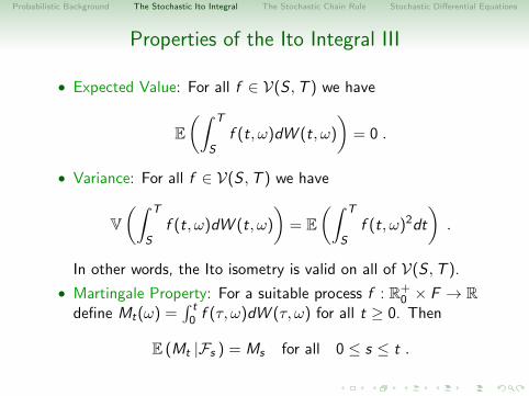
Properties of the Ito Integral III

• Expected Value: For all f ∈ V(S ,T ) we have

E(∫ T


)= 0 .

• Variance: For all f ∈ V(S ,T ) we have

V(∫ T


)= E

(∫ T

Sf (t, ω)2dt

).

In other words, the Ito isometry is valid on all of V(S ,T ).

• Martingale Property: For a suitable process f : R+0 × F → R

define Mt(ω) =∫ t

0 f (τ, ω)dW (τ, ω) for all t ≥ 0. Then

E (Mt |Fs ) = Ms for all 0 ≤ s ≤ t .


Properties of the Ito Integral IV

• Martingale Inequalities: Define Mt(ω) =∫ t

0 f (τ, ω)dW (τ, ω)for all t ≥ 0 as before, and assume without loss of generalitythat M is continuous with respect to t. Then for all λ,T > 0we have

P

(sup

0≤t≤T|Mt | ≥ λ

)≤ 1

λ2· E(M2

T

)=

1

λ2· E(∫ T

0f (s, ω)2 ds

),

as well as

E

(sup

0≤t≤TM2

t

)≤ 4E

(M2

T

)= 4E

(∫ T

0f (s, ω)2 ds

).


Properties of the Ito Integral V

• Gaussianity: If the integrand function f is deterministic, i.e.,if f is independent of ω, then the stochastic integral∫ T

Sf (t)dW (t, ω) is a Gaussian random variable

with

mean 0 and variance

∫ T

Sf (t)2dt .

If the integrands depends on ω, then in general the Itointegral is not a Gaussian random variable.


A First Example

We now demonstrate how the properties of the Ito integral can beused to show that∫ T

0W (t, ω)dW (t, ω) =

W (T , ω)2

2− T

2.

The idea is to approximate the integral by elementary processesin V(0,T ). For this, let 0 = t0 < . . . < tn = T denote apartition P of [0,T ] and consider the elementary process

fP(t, ω) =n−1∑k=0

W (tk , ω) · χ[tk ,tk+1)(t) ,

where χA(t) denotes the characteristic function of a set A.


A First Example

First we need to show that as max(tk+1 − tk)→ 0, the elementaryfunction fP converges to the Wiener process in V(0,T ). This canbe seen as follows:

‖fP −W ‖2V(0,T ) = E

(n−1∑k=0

∫ tk+1

tk

(W (tk , ω)−W (s, ω))2 ds

)

=n−1∑k=0

∫ tk+1

tk

E(

(W (s, ω)−W (tk , ω))2)ds

=n−1∑k=0

∫ tk+1

tk

(s − tk) ds =n−1∑k=0

(tk+1 − tk)2

2

→ 0 as long as max(tk+1 − tk)→ 0 .


A First Example

Finally we need that for max(tk+1 − tk)→ 0, the integral of theelementary function fP converges to (W (T )2 − T )/2 in L2(P),

since I[fP ]→∫ T

0 W (t, ω)dW (t, ω). This follows from

W (T )2 =n−1∑k=0

(W (tk+1)2 −W (tk)2

)=

n−1∑k=0

(W (tk+1)−W (tk))2

︸︷︷︸→ T

+ 2n−1∑k=0

W (tk) (W (tk+1)−W (tk))︸︷︷︸= I[fP ]→

∫ T0 W (t,ω)dW (t,ω)


Comments on the Ito Integral

• For integrands f which are adapted stochastic processes witha certain integrability condition, it is possible to define thestochastic Ito integral

∫ TS f (t, ω) dW (t, ω) with respect to the

Wiener process as a random variable in L2(P).

• The stochastic integral can not be defined path-wise, i.e., forfixed ω. It is constructed via a limit process in L2(P).

• Ito integration establishes a one-to-one correspondencebetween the integrand and the integral.

• The notion of the integral discussed here is inadequate for thevector-valued case, i.e., if one would like to integrate withrespect to multi-dimensional Brownian motion. For this, thecondition (ii) in the definition of V(S ,T ) has to be weakened.


3. The Stochastic Chain Rule

Just as in the deterministic setting, stochastic integrals are usuallynot computed through their definition, but by means of anassociated stochastic Ito calculus. Such a calculus should involveversions of a change of variable formula and integration by parts.For this, it is convenient to introduce the following notion.

Definition (Ito Processes)

A stochastic process X (t, ω) is called Ito process, if it satisfies anintegral equation of the form

X (t, ω) = X (0, ω) +

∫ t

0u(s, ω)ds +

∫ t

0v(s, ω)dW (s, ω) ,

for suitable adapted stochastic processes u and v . If X is an Itoprocess, the above integral identity is generally abbreviated as

dX (t) = udt + vdW (t) .


Gaussian Ito Processes

In general, Ito processes are not Gaussian processes. There is,however, one special case in which this is true.

Lemma (Gaussian Ito Processes)

Let X (t, ω) be an Ito processes satisfying dX (t) = udt + vdW (t)and assume that both u and v are deterministic functions of t.Furthermore, assume that X (0, ω) ≡ X0 is constant, i.e., we have

X (t, ω) = X0 +

∫ t

0u(s)ds +

∫ t

0v(s)dW (s, ω) .

Then X is a Gaussian process with independent increments and

E(X (t)) = X0 +

∫ t

0u(s)ds and V(X (t)) =

∫ t

0v(s)2ds .


Stochastic Chain Rule

Theorem (Stochastic Chain Rule, Ito’s Formula)

Let X be an Ito process with dX (t) = udt + vdW (t), andlet g(t, x) denote a C 2-function. Then the process

Y (t, ω) = g(t,X (t, ω))

is again an Ito process and we have

dY (t) =∂g

∂t(t,X (t))dt +

∂g

∂x(t,X (t))dX (t)

+1

2

∂2g

∂x2(t,X (t)) · (dX (t))2 ,

where (dX (t))2 is computed using the rules dW (t) · dW (t) = dtand dt · dt = dt · dW (t) = dW (t) · dt = 0.



Remarks:

• Notice that Ito’s formula can be written equivalently in thefollowing form

dY (t) =

(∂g

∂t(t,X ) + u · ∂g

∂x(t,X ) +

v2

2· ∂

2g

∂x2(t,X )

)dt

+ v · ∂g∂x

(t,X )dW (t) ,

where we omitted the argument from the Ito process X .

• While the formula reduces to the classical chain rule in thedeterministic case v ≡ 0, the stochastic version introduces anadditional term which depends on ∂2g/∂x2.



• Ito’s formula is basically proved by assuming that u and v areelementary processes with respect to the same partition of theunderlying interval, and using a Taylor approximation on eachof the subintervals. Among other things, this leads to terms ofthe form

n−1∑k=0

v(tk)2 · ∂2g

∂x2(tk ,X (tk)) · (W (tk+1)−W (tk))2

One can show that in the space L2(P), this random variableconverges to ∫ t

0v(s)2 · ∂

2g

∂x2(s,X (s, ω))ds

as max(tk+1 − tk)→ 0, which accounts for the extra term.


Example:

∫ T

0

W (t, ω)dW (t, ω)

From the deterministic theory we guess that the integral shouldinclude a term of the form W (T )2/2. Thus, we consider

dX (t) = 0dt + 1dW (t) and g(t, x) =x2

2.

For Y (t) = g(t,X (t)) = W (t)2/2 Ito’s formula then implies

dY (t) =

∂g

∂t︸︷︷︸=0

+ u · ∂g∂x︸︷︷︸

=0

+v2

2· ∂

2g

∂x2︸︷︷︸=1/2

dt + v · ∂g∂x

dW (t)︸︷︷︸=W (t)dW (t)

,

which furnishes

W (T )2

2=

T

2+

∫ T

0W (t, ω) dW (t, ω) .


Example:

∫ T

0

t dW (t, ω)

From the deterministic theory we guess that the integral shouldinclude a term of the form T ·W (T ). Thus, we consider

dX (t) = 0dt + 1dW (t) and g(t, x) = tx .

For Y (t) = g(t,X (t)) = t ·W (t) Ito’s formula then implies

dY (t) =

∂g

∂t︸︷︷︸=W (t)

+ u · ∂g∂x︸︷︷︸

=0

+v2

2· ∂

2g

∂x2︸︷︷︸=0

dt + v · ∂g∂x

dW (t)︸︷︷︸=t dW (t)

,

which furnishes

T ·W (T ) =

∫ T

0W (t, ω) dt +

∫ T

0t dW (t, ω) .


Generalizations of Ito’s Formula

Ito’s formula can be generalized in a number of ways to cover thecase of vector-valued processes X (t, ω) and vector-valued Brownianmotions B(t, ω). We only mention one such generalization.

Theorem (Ito’s Formula for Multiple Ito Processes)

Let Xk , k = 1, . . . , d , denote a family of Ito processes with respectto the same Wiener process, given by dXk(t) = ukdt + vkdW (t),and let g(t, x1, . . . , xd) denote a C 2-function. Then the processY (t, ω) = g(t,X1(t, ω), . . . ,Xd(t, ω)) is an Ito process with

dY (t) =∂g

∂tdt +

d∑k=1

∂g

∂xkdXk(t) +

1

2

d∑k,`=1

∂2g

∂xk∂x`dXk(t)dX`(t),

where dXk(t)dX`(t) = vkv`dt, and the partial derivatives of g areevaluated at (t,X1(t, ω), . . . ,Xd(t, ω)).


Stochastic Integration by Parts

Specifically for g(t, x1, x2) = x1 · x2 one obtains the stochasticversion of integration by parts.

Theorem (Stochastic Integration by Parts Formula)

Let X1,X2 denote two Ito processes with respect to the sameWiener process, given by dXk(t) = ukdt + vkdW (t) for k = 1, 2.Then their product X1 · X2 is again an Ito process and we have

d (X1(t) · X2(t)) = X1dX2 + X2dX1 + v1v2dt .

Notice in particular that if either X1 or X2 is an Ito process withpaths of bounded variation, then the classical deterministicintegration by parts formula holds.


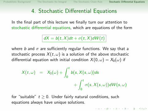
4. Stochastic Differential Equations

In the final part of this lecture we finally turn our attention tostochastic differential equations, which are equations of the form

dX = b(t,X )dt + σ(t,X )dW (t)

where b and σ are sufficiently regular functions. We say that astochastic process X (t, ω) is a solution of the above stochasticdifferential equation with initial condition X (0, ω) = X0(ω) if

X (t, ω) = X0(ω) +

∫ t

0b(s,X (s, ω))ds

+

∫ t

0σ(s,X (s, ω))dW (s, ω)

for “suitable” t ≥ 0. Under fairly natural conditions, suchequations always have unique solutions.


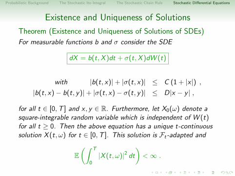
Existence and Uniqueness of Solutions

Theorem (Existence and Uniqueness of Solutions of SDEs)

For measurable functions b and σ consider the SDE


with |b(t, x)|+ |σ(t, x)| ≤ C (1 + |x |) ,|b(t, x)− b(t, y)|+ |σ(t, x)− σ(t, y)| ≤ D|x − y | ,

for all t ∈ [0,T ] and x , y ∈ R. Furthermore, let X0(ω) denote asquare-integrable random variable which is independent of W (t)for all t ≥ 0. Then the above equation has a unique t-continuoussolution X (t, ω) for t ∈ [0,T ]. This solution is Ft-adapted and

E(∫ T

0|X (t, ω)|2 dt

)<∞ .


Remarks and Generalizations

• The existence and uniqueness result can be proved via Picarditeration, similarly to the deterministic situation. Thenecessary solution estimates make use of the martingaleinequalities mentioned as one of the properties of thestochastic integral.

• An analogous existence and uniqueness theorem holds in thevector-valued case X (t, ω) ∈ Rn for equations of the form

dX = b(t,X )dt +m∑

k=1

σk(t,X )dWk(t) ,

where the Wiener processes W1, . . . ,Wm are independent.


Remarks and Generalizations

• One can think of the stochastic differential equation


as being a perturbation of the deterministic equation

X = b(t,X ) .

This latter equation is perturbed by additive noise if σ doesnot depend on X , and it is perturbed by multiplicative noiseif σ does depend explicitly on X .


A Noisy Population Growth Model

As a first example we consider the noisy population growth model

dZ = aZdt + bZdW (t) with Z (0, ω) = Z0 ∈ R

where a and b are real constants. This is the usual deterministicexponential growth model perturbed by multiplicative white noise.

To find the solution, we use the intuition from the deterministicsituation to suggest that the solution might involve the term

eαt+βW (t,ω) for certain α, β ∈ R .

Therefore, it seems natural to apply Ito’s formula to the Itoprocess X (t, ω) = W (t, ω) which satisfies dX = 0dt + 1dW (t),and the nonlinearity g(t, x) = exp(αt + βx).



For Y (t, ω) = g(t,X (t, ω)) = eαt+βW (t,ω) Ito’s formula implies

dY (t) =

∂g

∂t︸︷︷︸=αY

+ u · ∂g∂x︸︷︷︸

=0

+v2

2· ∂

2g

∂x2︸︷︷︸=β2Y /2

dt + v · ∂g∂x

dW (t)︸︷︷︸=βYdW (t)

,

which shows that Y (t, ω) solves the stochastic differential equation

dY =

(α +

β2

2

)Ydt + βYdW (t) .

Comparing this with the form of the noisy population growthmodel furnishes

Z (t, ω) = Z0 · e(a− b2

2

)t+bW (t,ω)



• Note that due to

Z (t, ω) = Z0 +

∫ t

0aZ (s, ω)ds +

∫ t

0bZ (s, ω)dW (s, ω)

and the properties of the Ito integral we have

E (Z (t)) = Z0 · eat for all t ≥ 0 .

• The typical path behavior deviates from the deterministiccase. For almost all paths of the Wiener process we have

limt→∞

W (t, ω)

t= 0 ,

which means that typical paths of Z satisfy

Z (t, ω) = Z0e

(a− b2

2

)t+bW (t,ω) ∼ Z0e

(a− b2

2

)t

for t →∞ .



• One can also determine the variance of the solutionprocess Z (t, ω). Note that we have

Z (t, ω)2 = Z 20 · e(2a−b2)t+2bW (t,ω) ,

and as before this implies

d(Z 2)

=

((2a− b2

)+

(2b)2

2

)Z 2dt + 2bZ 2dW (t) ,

and therefore

E(Z (t)2

)= Z 2

0 · e(2a+b2)t for all t ≥ 0 .

This finally implies

V (Z (t)) = Z 20 · e2at ·

(eb

2t − 1)

for all t ≥ 0 .


The Ornstein-Uhlenbeck Process

Our second example is the so-called Langevin equation

dZ = −aZdt + bdW (t) with Z (0, ω) = Z0 ∈ R

where a 6= 0 and b are real constants. This is a deterministic linearequation perturbed by additive white noise, and its solution processis called the Ornstein-Uhlenbeck process.

In the deterministic setting, equations of this type are solved bymoving the term −aZdt to the left, multiplying the equation bythe integrating factor eat , and integrating to obtain Z (t)eat on theleft-hand side. This suggests that in the stochastic case, it makessense to determine whether the process eat · Z (t, ω) is an Itoprocess, i.e., apply Ito’s formula to X (t, ω) = Z (t, ω) with thetransformation g(t, x) = eat · x , where u = −aZ and v = b in therepresentation dX = udt + vdW (t).



For Y (t, ω) = g(t,X (t, ω)) = eatZ (t, ω) Ito’s formula implies

dY (t) =

∂g

∂t︸︷︷︸=aeatZ

+ u · ∂g∂x︸︷︷︸

=−aZ ·eat

+v2

2· ∂

2g

∂x2︸︷︷︸=0

dt + v · ∂g∂x

dW (t)︸︷︷︸=b·eatdW (t)

,

which shows that Y (t, ω) satisfies

Y (t, ω)− Y (0, ω)︸︷︷︸= eatZ(t,ω)−Z0

=

∫ t

0beasdW (s, ω) ,

and the Ornstein-Uhlenbeck process is therefore given by

Z (t, ω) = Z0 · e−at + b ·∫ t

0e−a(t−s)dW (s, ω)



• Note that the explicit formula for the Ornstein-Uhlenbeckprocess is exactly what one would obtain by applying thestandard deterministic variation of constants formula to theLangevin equation.

• In contrast to the noisy population growth model discussedbefore, the Ornstein-Uhlenbeck process fits into the categoryof Gaussian Ito processes which was discussed at thebeginning of this section. Thus, the Ornstein-Uhlenbeckprocess is a Gaussian process with independent increments.

• Due to the properties of the Ito integral we have

E (Z (t)) = Z0 · e−at for all t ≥ 0 .



• One can also easily determine the variance of theOrnstein-Uhlenbeck process Z (t, ω). Note that we have

V (Z (t)) = E(Z (t, ω)− Z0 · e−at

)2

= E(be−at ·

∫ t

0easdW (s, ω)

)2

= b2e−2at · V(∫ t

0easdW (s, ω)

)= b2e−2at ·

∫ t

0e2asds .

This finally implies

V (Z (t)) =b2

2a·(1− e−2at

)for all t ≥ 0 .


Thank You!

References:

• Bernt Oksendal: Stochastic Differential Equations: AnIntroduction with Applications. Springer-Verlag, 2010.

• Ludwig Arnold: Stochastic Differential Equations: Theory andApplications. Dover Publications, 2013.

• Lawrence C. Evans: An Introduction to Stochastic DifferentialEquations. Online Lecture Notes, 2006.

Date post:	04-Jun-2018
Category:	Documents
Upload:	doliem
View:	225 times
Download:	0 times

An Introduction to Stochastic Ordinary Differential ... · An Introduction to Stochastic Ordinary...

Documents