An Introduction to the Theory of Lattices and …jhs/Presentations/WyomingLattices.pdfTheory of...

An Introduction to theTheory of Lattices and

Applications to CryptographyJoseph H. SilvermanBrown University and

NTRU Cryptosystems, Inc.

Summer School onComputational Number Theory and

Applications to CryptographyUniversity of Wyoming

June 19 – July 7, 2006

0

An Introduction to the Theory of Lattices

Outline

• Introduction• Lattices and Lattice Problems• Fundamental Lattice Theorems• Lattice Reduction and the LLL Algorithm• Knapsack Cryptosystems and Lattice Cryptanaly-

sis• Lattice-Based Cryptography• The NTRU Public Key Cryptosystem• Convolution Modular Lattices and NTRU Lattices• Further Reading

An Introduction to the Theory of Lattices – 1–


Public Key Cryptography andHard Mathematical Problems

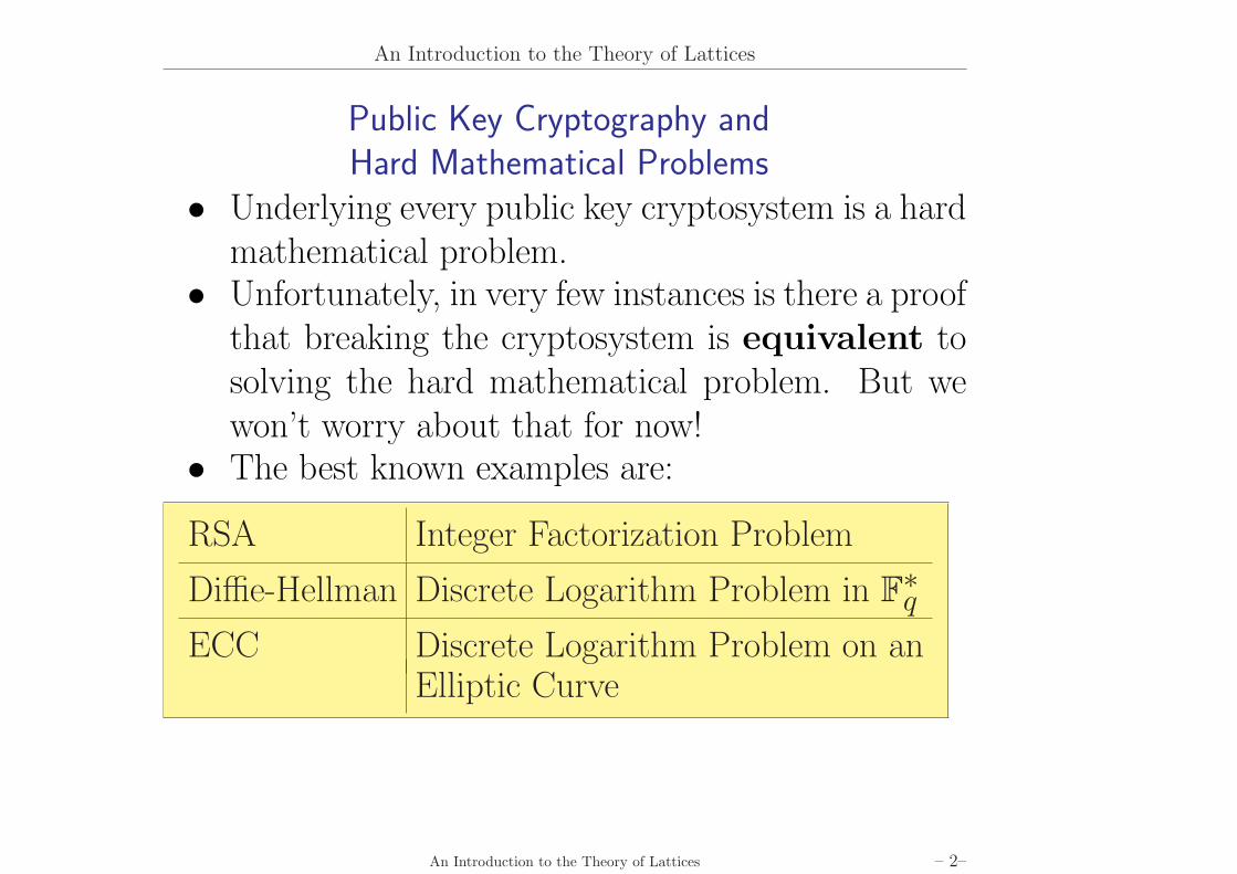
• Underlying every public key cryptosystem is a hardmathematical problem.

• Unfortunately, in very few instances is there a proofthat breaking the cryptosystem is equivalent tosolving the hard mathematical problem. But wewon’t worry about that for now!

• The best known examples are:

RSA Integer Factorization Problem

Diffie-Hellman Discrete Logarithm Problem in F∗qECC Discrete Logarithm Problem on an

Elliptic Curve



A Different Hard Problem for Cryptography

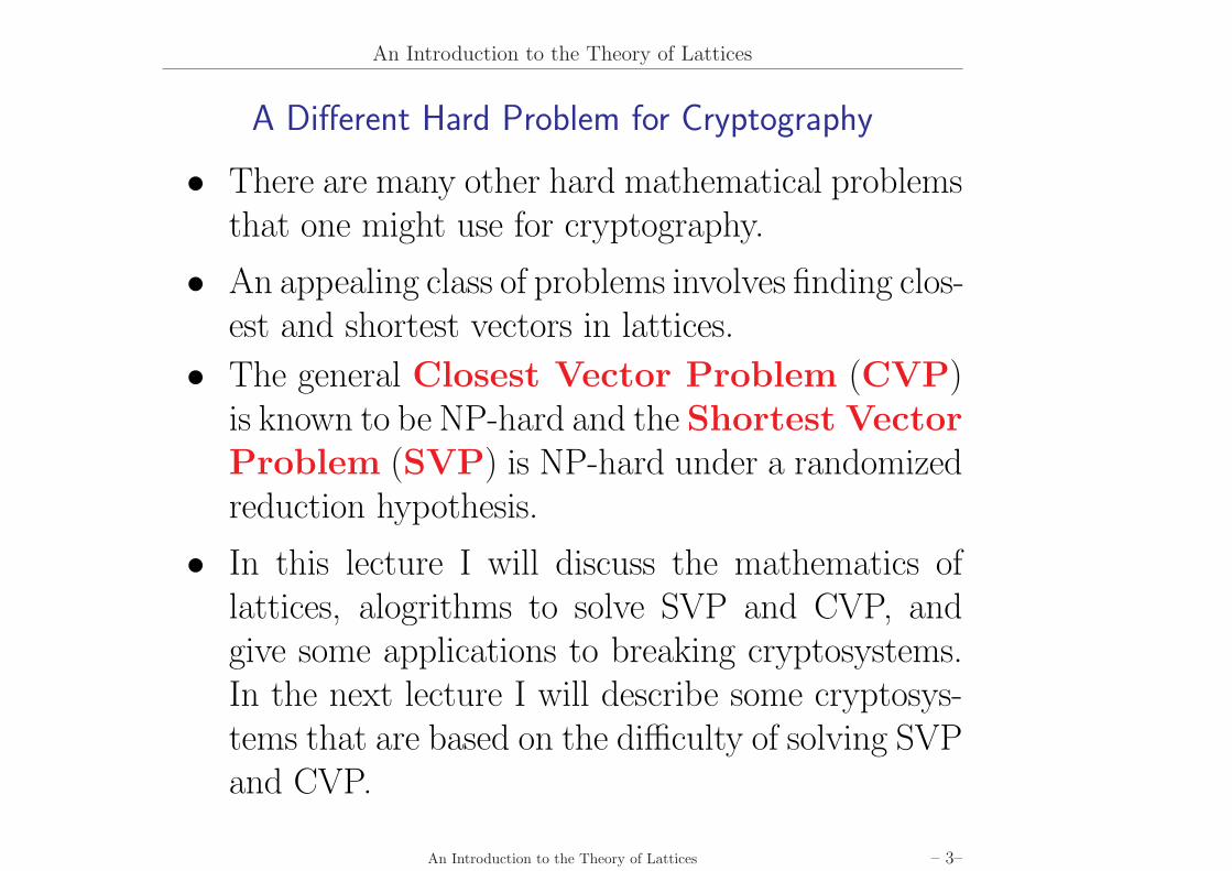
• There are many other hard mathematical problemsthat one might use for cryptography.

• An appealing class of problems involves finding clos-est and shortest vectors in lattices.

• The general Closest Vector Problem (CVP)is known to be NP-hard and the Shortest VectorProblem (SVP) is NP-hard under a randomizedreduction hypothesis.

• In this lecture I will discuss the mathematics oflattices, alogrithms to solve SVP and CVP, andgive some applications to breaking cryptosystems.In the next lecture I will describe some cryptosys-tems that are based on the difficulty of solving SVPand CVP.


Latticesand

Lattice Problems

Lattices and Lattice Problems

Lattices — Definition and Notation

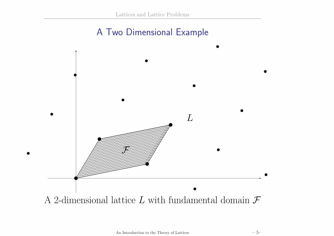
Definition. A lattice L of dimension n is a maximaldiscrete subgroup of Rn.

Equivalently, a lattice is the Z-linear span of a set of nlinearly independent vectors:

L = {a1v1 + a2v2 + · · · + anvn : a1, a2, . . . , an ∈ Z}.The vectors v1, . . . ,vn are a Basis for L. Latticeshave many bases. Some bases are “better” than others.

A fundamental domain for the quotient Rn/L isthe set

F(L) = {t1v1 + t2v2 + · · · + tnvn : 0 ≤ ti < 1}.The Discriminant (or “volume”) of L is

Disc(L) = Volume(F(L)) = det(v1|v2| · · · |vn

).



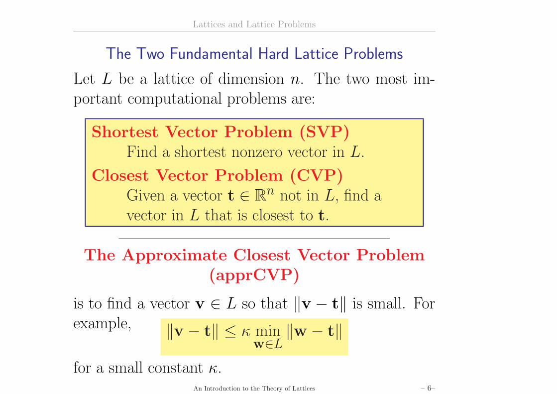
A Two Dimensional Example

··········

··········

··········

··········

··········

··········

··········

··········

··········

··········

··········

··········

··········

··········

··········

··········

··········

··········

··········

··········

··········

··········

··········

··········

··········

··········

··········

··········

··········

··········

··········

··········

··········

··········

··········

··········

··········

··········

··········

ÃÃÃÃÃÃÃÃÃÃÃÃÃÃÃÃÃÃÃ






















x

x

x

x

··········

ÃÃÃÃÃÃÃÃÃÃÃÃÃÃÃÃÃÃÃ··········


v

v

vv

vv

v

v

vv

v

v6

-

F

L

A 2-dimensional lattice L with fundamental domain F



The Two Fundamental Hard Lattice Problems

Let L be a lattice of dimension n. The two most im-portant computational problems are:

Shortest Vector Problem (SVP)Find a shortest nonzero vector in L.

Closest Vector Problem (CVP)Given a vector t ∈ Rn not in L, find avector in L that is closest to t.

The Approximate Closest Vector Problem(apprCVP)

is to find a vector v ∈ L so that ‖v − t‖ is small. Forexample, ‖v − t‖ ≤ κ min

w∈L‖w − t‖

for a small constant κ.An Introduction to the Theory of Lattices – 6–


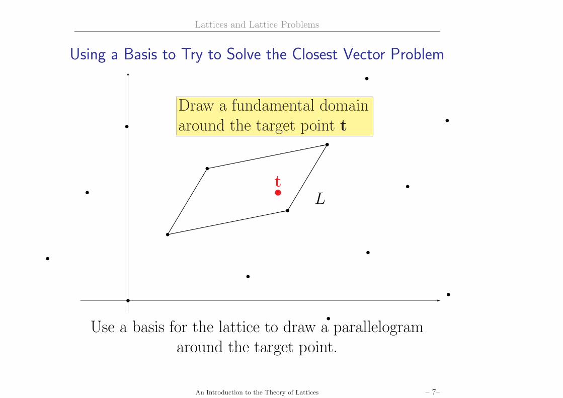
Using a Basis to Try to Solve the Closest Vector Problem

t

t

t

t

t

t

tt

tt

t

t

tt

t

··········



tx

Draw a fundamental domainaround the target point t

6

-

L

Use a basis for the lattice to draw a parallelogramaround the target point.



Using a Basis to Try to Solve the Closest Vector Problem

t

t

t

t

tt

t

t

tt

t

··········



tx

x

v

The vertex v that is closestto t is a candidate for(approximate) closest vector

6

-

L

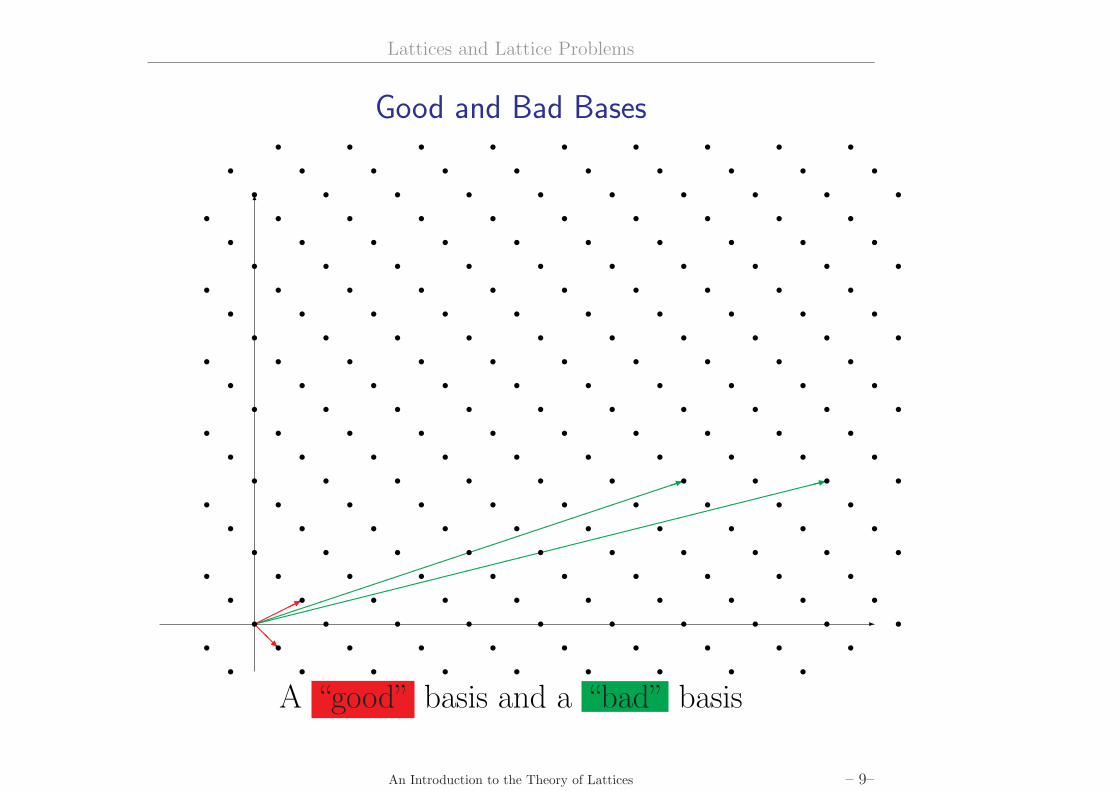
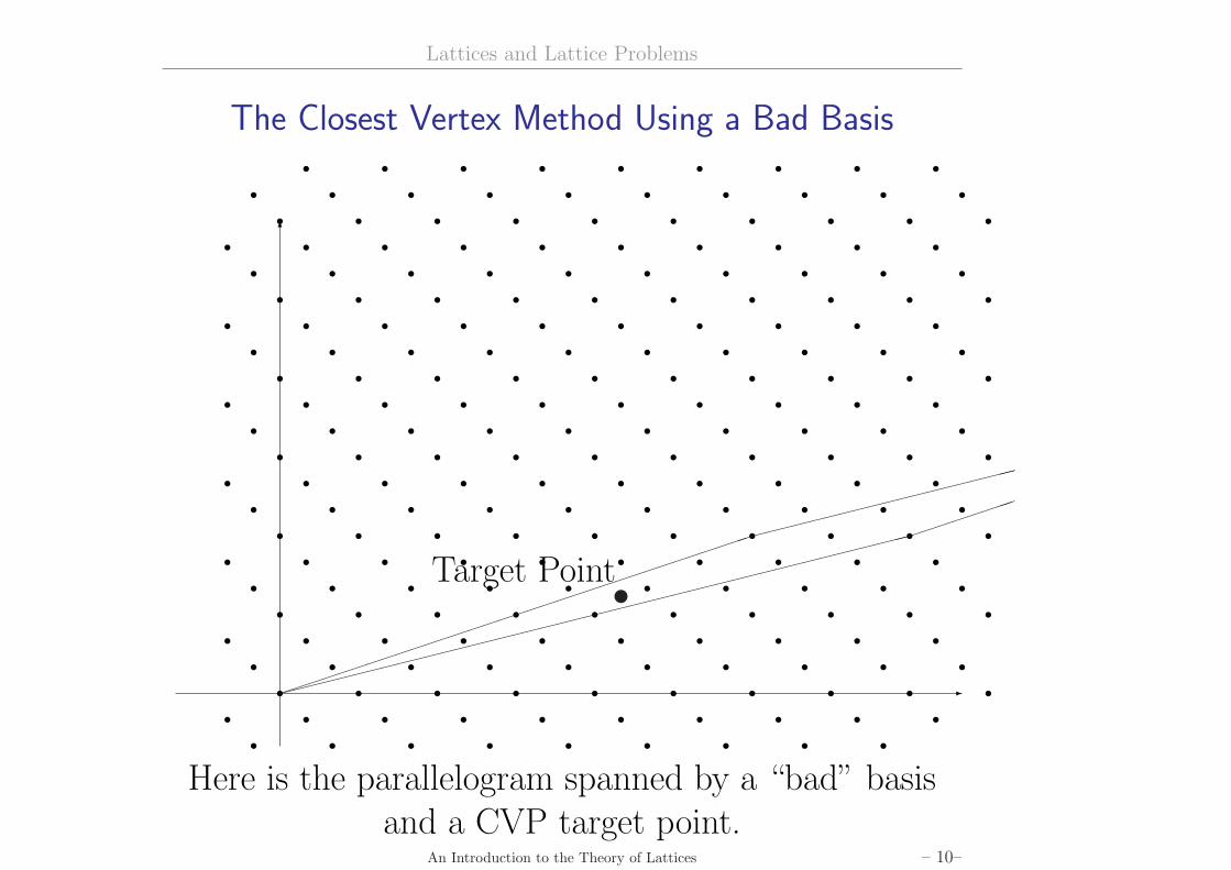
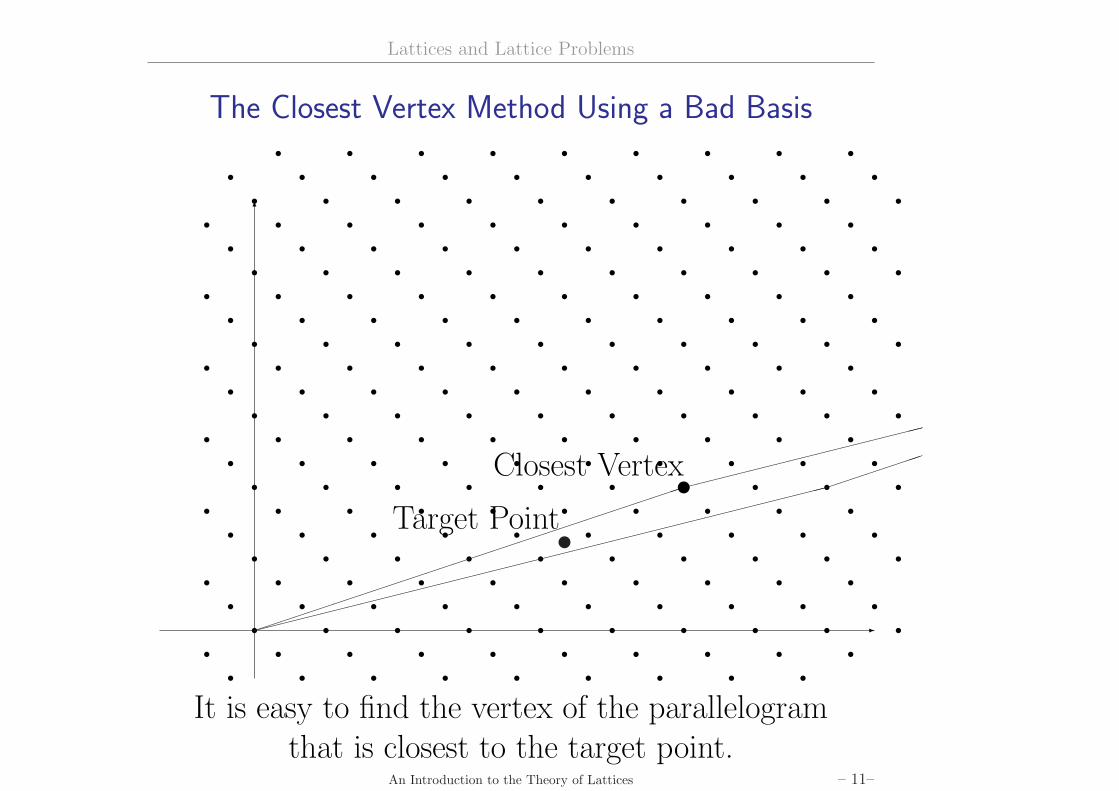
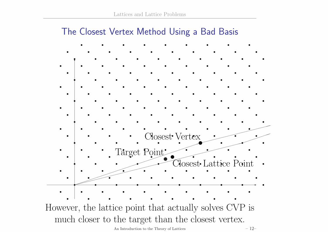
The vertex v of the fundamental domain that is closestto t will be a close lattice point if the basis is “good”,meaning if the basis consists of short vectors that arereasonably orthogonal to one another.



Good and Bad Bases

»»»»»»»»»»»»»»»»»»»»»»»»»»»»»»»»»»»»»»»»»»»»:

³³³³³³³³³³³³³³³³³³³³³³³³³³³³³³³³³1

©©©©*

@@Rs

ss

ss

ss

ss

ss

ss

ss

ss

ss

ss

ss

ss

ss

ss

s

ss

ss

ss

ss

ss

ss

ss

s

ss

ss

ss

ss

ss

ss

ss

s

ss

ss

ss

ss

ss

ss

ss

s

ss

ss

ss

ss

ss

ss

ss

ss

ss

ss

ss

ss

ss

s

ss

ss

ss

ss

ss

s

ss

ss

ss

ss

ss

ss

ss

ss

ss

ss

ss

ss

s

ss

ss

s

ss

ss

ss

ss

ss

ss

ss

ss

ss

ss

s

ss

ss

ss

ss

ss

ss

s

ss

ss

ss

ss

ss

ss

ss

ss

ss

ss

ss

ss

ss

ss

ss

s

ss

ss

ss

s

ss

ss

ss

ss

ss

ss

s

6

-

A “good” basis and a “bad” basis



The Closest Vertex Method Using a Bad Basis

ss

ss

ss

ss

ss

ss

ss

s

ss

ss

ss

ss

ss

ss

ss

s

ss

ss

ss

ss

ss

ss

ss

s

ss

ss

ss

ss

ss

ss

ss

s

ss

ss

ss

ss

ss

ss

ss

s

ss

ss

ss

ss

ss

ss

ss

ss

ss

ss

ss

ss

ss

s

ss

ss

ss

ss

ss

s

ss

ss

ss

ss

ss

ss

ss

ss

ss

ss

ss

ss

s

ss

ss

s

ss

ss

ss

ss

ss

ss

ss

ss

ss

ss

s

ss

ss

ss

ss

ss

ss

s

ss

ss

ss

ss

ss

ss

ss

ss

ss

ss

ss

ss

ss

ss

ss

s

ss

ss

ss

s

ss

ss

ss

ss

ss

ss

s

6

-»»»»»»»»»»»»»»»»»»»»»»»»»»»»»»»»»»»»»»»»»»»»

³³³³³³³³³³³³³³³³³³³³³³³³³³³³³³³³³»»»»»»»»»»»»»»»»»»»

³³³³³³³³

xTarget Point

Here is the parallelogram spanned by a “bad” basisand a CVP target point.




ss

ss

ss

ss

ss

ss

ss

s

ss

ss

ss

ss

ss

ss

ss

s

ss

ss

ss

ss

ss

ss

ss

s

ss

ss

ss

ss

ss

ss

ss

s

ss

ss

ss

ss

ss

ss

ss

s

ss

ss

ss

ss

ss

ss

ss

ss

ss

ss

ss

ss

ss

s

ss

ss

ss

ss

ss

s

ss

ss

ss

ss

ss

ss

ss

ss

ss

ss

ss

ss

s

ss

ss

s

ss

ss

ss

ss

ss

ss

ss

ss

ss

ss

s

ss

ss

ss

ss

ss

ss

s

ss

ss

ss

ss

ss

ss

ss

ss

ss

ss

ss

ss

ss

ss

ss

s

ss

ss

ss

s

ss

ss

ss

ss

ss

ss

s

6

-»»»»»»»»»»»»»»»»»»»»»»»»»»»»»»»»»»»»»»»»»»»»

³³³³³³³³³³³³³³³³³³³³³³³³³³³³³³³³³»»»»»»»»»»»»»»»»»»»

³³³³³³³³

xTarget Point

xClosest Vertex

It is easy to find the vertex of the parallelogramthat is closest to the target point.




ss

ss

ss

ss

ss

ss

ss

s

ss

ss

ss

ss

ss

ss

ss

s

ss

ss

ss

ss

ss

ss

ss

s

ss

ss

ss

ss

ss

ss

ss

s

ss

ss

ss

ss

ss

ss

ss

s

ss

ss

ss

ss

ss

ss

ss

ss

ss

ss

ss

ss

ss

s

ss

ss

ss

ss

ss

s

ss

ss

ss

ss

ss

ss

ss

ss

ss

ss

ss

ss

s

ss

ss

s

ss

ss

ss

ss

ss

ss

ss

ss

ss

ss

s

ss

ss

ss

ss

ss

ss

s

ss

ss

ss

ss

ss

ss

ss

ss

ss

ss

ss

ss

ss

ss

ss

s

ss

ss

ss

s

ss

ss

ss

ss

ss

ss

s

6

-»»»»»»»»»»»»»»»»»»»»»»»»»»»»»»»»»»»»»»»»»»»»

³³³³³³³³³³³³³³³³³³³³³³³³³³³³³³³³³»»»»»»»»»»»»»»»»»»»

³³³³³³³³

xTarget Point

xClosest Vertex

x

Closest Lattice Point

However, the lattice point that actually solves CVP ismuch closer to the target than the closest vertex.



Theory and Practice

Lattices, SVP and CVP, have been intensively studiedfor more than 100 years, both as intrinsic mathemati-cal problems and for applications in pure and appliedmathematics, physics and cryptography.

The theoretical study of lattices is often called the

Geometry of Numbers,

a name bestowed on it by Minkowski in his 1910 bookGeometrie der Zahlen.

The practical process of finding short(est) or close(st)vectors in lattices is called Lattice Reduction.

Lattice reduction methods have been extensively devel-oped for applications to number theory, computer alge-bra, discrete mathematics, applied mathematics, com-binatorics, cryptography,. . .


Fundamental Lattice Theorems


How Orthogonal is a Basis of a Lattice?

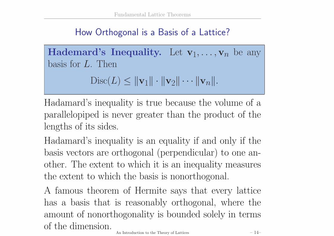
Hademard’s Inequality. Let v1, . . . ,vn be anybasis for L. Then

Disc(L) ≤ ‖v1‖ · ‖v2‖ · · · ‖vn‖.

Hadamard’s inequality is true because the volume of aparallelopiped is never greater than the product of thelengths of its sides.

Hadamard’s inequality is an equality if and only if thebasis vectors are orthogonal (perpendicular) to one an-other. The extent to which it is an inequality measuresthe extent to which the basis is nonorthogonal.

A famous theorem of Hermite says that every latticehas a basis that is reasonably orthogonal, where theamount of nonorthogonality is bounded solely in termsof the dimension.



A Fundamental Lattice Theorem from the 19th Century

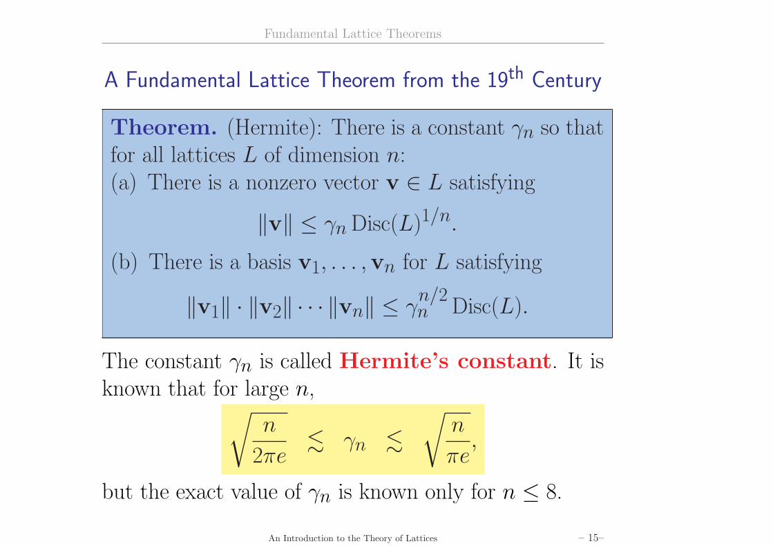
Theorem. (Hermite): There is a constant γn so thatfor all lattices L of dimension n:(a) There is a nonzero vector v ∈ L satisfying

‖v‖ ≤ γn Disc(L)1/n.

(b) There is a basis v1, . . . ,vn for L satisfying

‖v1‖ · ‖v2‖ · · · ‖vn‖ ≤ γn/2n Disc(L).

The constant γn is called Hermite’s constant. It isknown that for large n,√

n

2πe. γn .

√n

πe,

but the exact value of γn is known only for n ≤ 8.



Finding Points in Lattices — A Theoretical Result

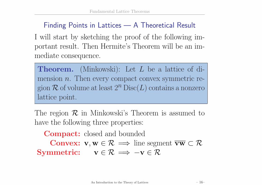
I will start by sketching the proof of the following im-portant result. Then Hermite’s Theorem will be an im-mediate consequence.

Theorem. (Minkowski): Let L be a lattice of di-mension n. Then every compact convex symmetric re-gionR of volume at least 2n Disc(L) contains a nonzerolattice point.

The region R in Minkowski’s Theorem is assumed tohave the following three properties:

Compact: closed and boundedConvex: v,w ∈ R =⇒ line segment vw ⊂ R

Symmetric: v ∈ R =⇒ −v ∈ R



Proof of Minkowski’s Theorem

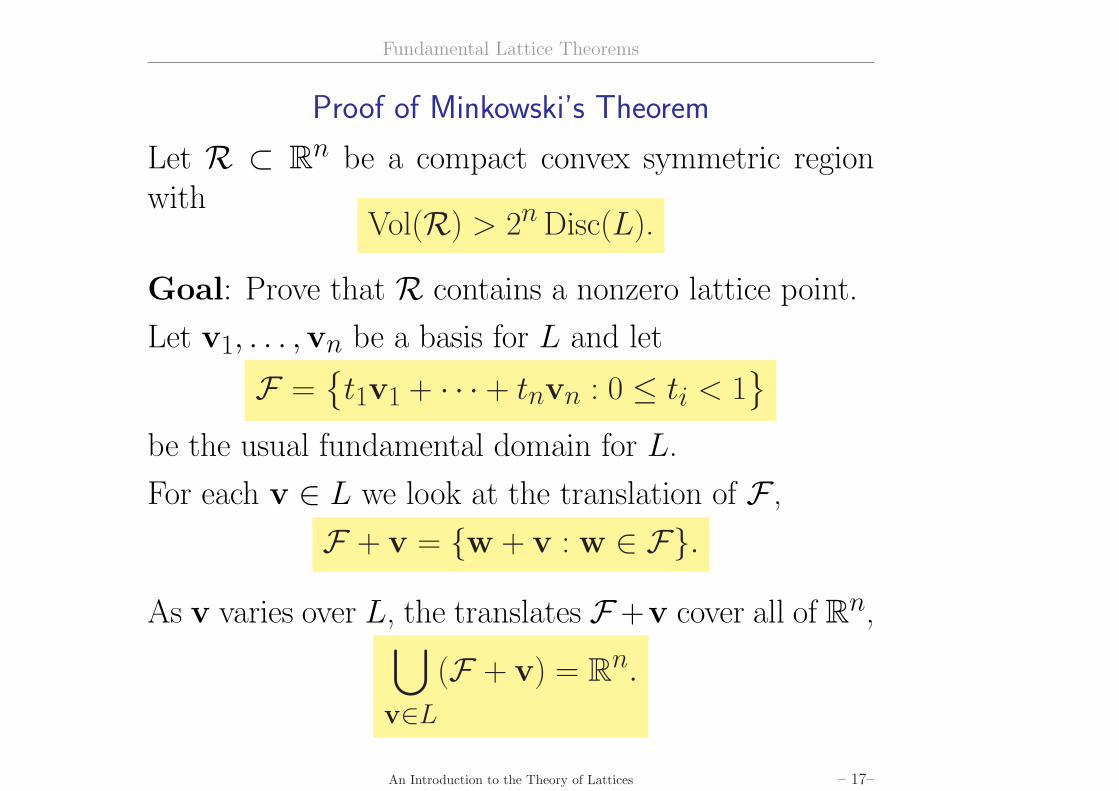
Let R ⊂ Rn be a compact convex symmetric regionwith

Vol(R) > 2n Disc(L).

Goal: Prove that R contains a nonzero lattice point.

Let v1, . . . ,vn be a basis for L and let

F ={t1v1 + · · · + tnvn : 0 ≤ ti < 1

}

be the usual fundamental domain for L.

For each v ∈ L we look at the translation of F ,

F + v = {w + v : w ∈ F}.

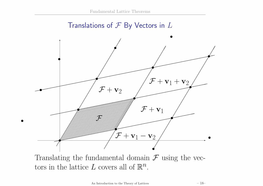
As v varies over L, the translates F +v cover all of Rn,⋃

v∈L

(F + v) = Rn.



Translations of F By Vectors in L

··········

··········

··········

··········

··········

··········

··········

··········

··········

··········

··········

··········

··········

··········

··········

··········

··········

··········

··········

··········

··········

··········

··········

··········

··········

··········

··········

··········

··········

··········

··········

··········

··········

··········

··········

··········

··········

··········

··········























v

v

v

v

···································

··································

··································

ÃÃÃÃÃÃÃÃÃÃÃÃÃÃÃÃÃÃÃÃÃÃÃÃÃÃÃÃÃÃÃÃÃÃÃÃÃÃÃÃÃÃÃÃÃÃÃÃÃÃÃÃÃÃÃÃÃÃÃÃÃÃÃÃÃÃÃÃÃÃÃÃÃÃÃÃÃÃÃÃÃÃÃÃÃÃÃÃÃÃÃÃÃÃÃÃÃ

ÃÃÃÃÃÃÃÃÃÃÃÃÃÃÃÃÃÃÃÃÃÃÃÃÃÃÃÃÃÃÃÃÃÃÃÃÃÃÃÃÃÃÃÃÃÃÃÃÃÃÃÃÃÃÃÃÃÃ

v

v

vv

vv

v

v

vv

v

v6

-

FF + v1

F + v2

F + v1 + v2

F + v1 − v2

Translating the fundamental domain F using the vec-tors in the lattice L covers all of Rn.



Proof of Minkowski’s Theorem (continued)

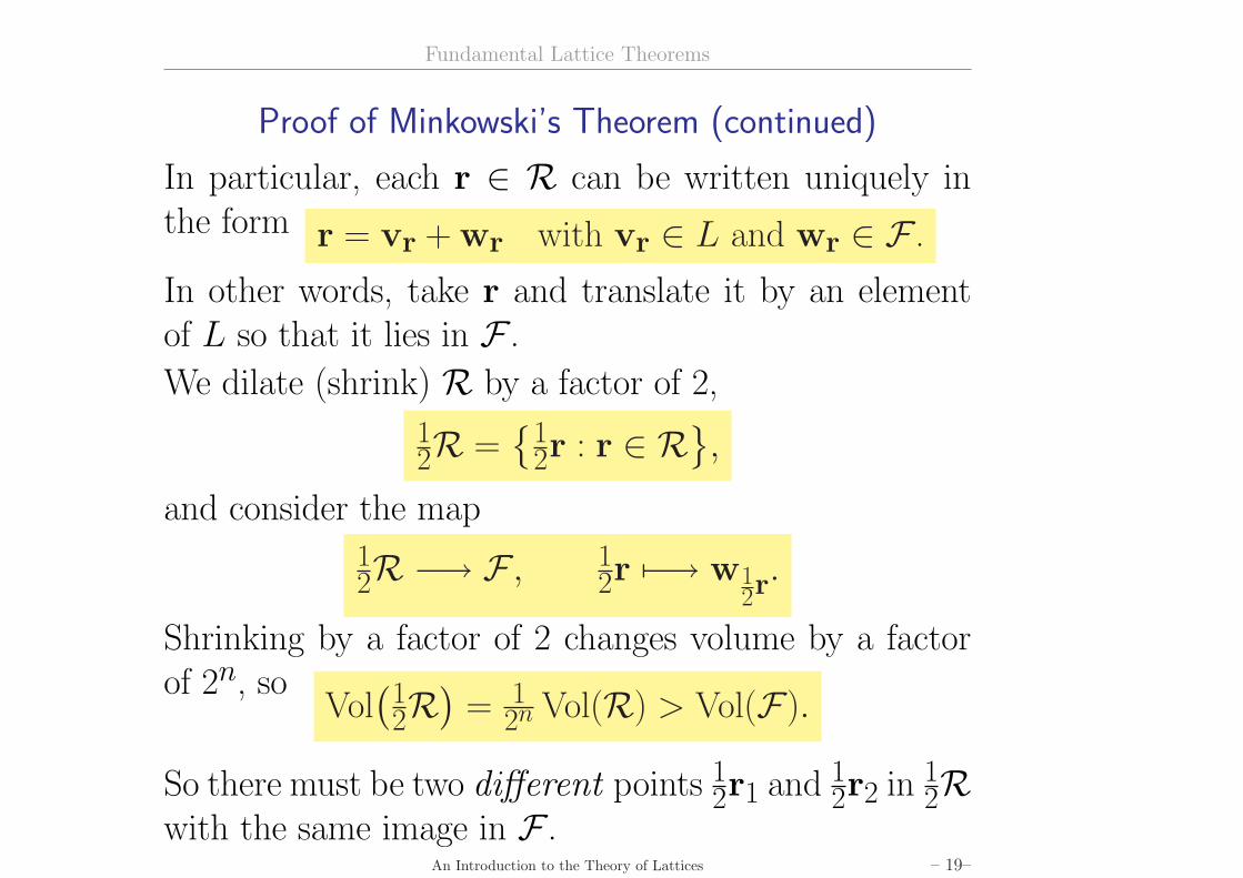
In particular, each r ∈ R can be written uniquely inthe form r = vr + wr with vr ∈ L and wr ∈ F .

In other words, take r and translate it by an elementof L so that it lies in F .

We dilate (shrink) R by a factor of 2,

12R =

{12r : r ∈ R}

,

and consider the map

12R −→ F , 1

2r 7−→ w12r

.

Shrinking by a factor of 2 changes volume by a factorof 2n, so

Vol(

12R

)= 1

2n Vol(R) > Vol(F).

So there must be two different points 12r1 and 1

2r2 in 12R

with the same image in F .An Introduction to the Theory of Lattices – 19–


Proof of Minkowski’s Theorem (continued)

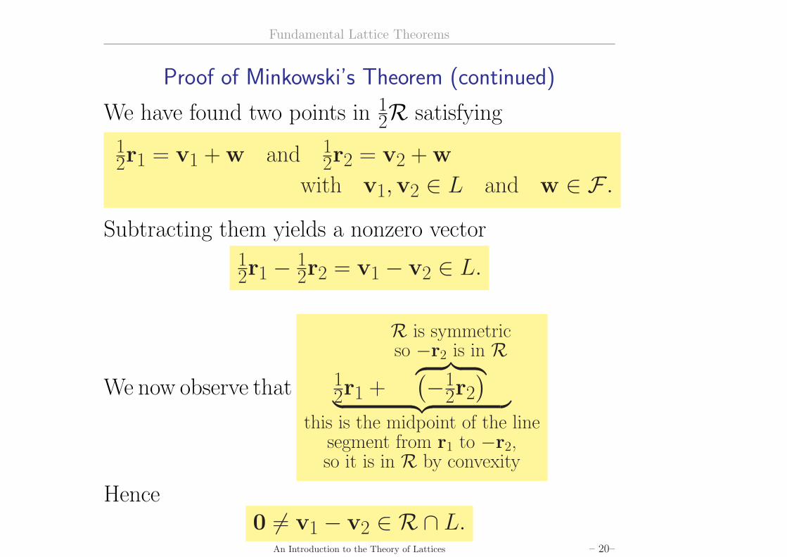
We have found two points in 12R satisfying

12r1 = v1 + w and 1

2r2 = v2 + w

with v1,v2 ∈ L and w ∈ F .

Subtracting them yields a nonzero vector

12r1 − 1

2r2 = v1 − v2 ∈ L.

We now observe that 12r1 +

R is symmetricso −r2 is in R︷︸︸︷(−1

2r2)

︸︷︷︸this is the midpoint of the line

segment from r1 to −r2,so it is in R by convexity

Hence0 6= v1 − v2 ∈ R ∩ L.



Proof of Minkowski’s Theorem (finale)

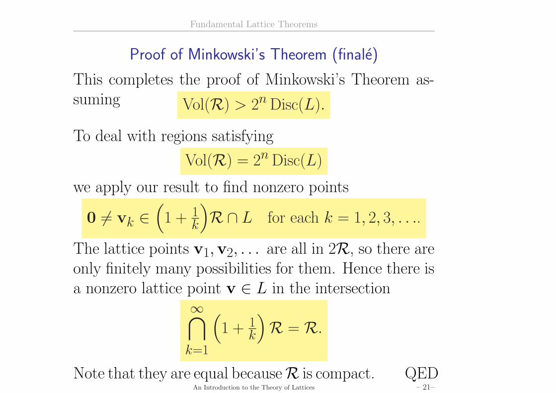
This completes the proof of Minkowski’s Theorem as-suming Vol(R) > 2n Disc(L).

To deal with regions satisfying

Vol(R) = 2n Disc(L)

we apply our result to find nonzero points

0 6= vk ∈(1 + 1

k

)R∩ L for each k = 1, 2, 3, . . ..

The lattice points v1,v2, . . . are all in 2R, so there areonly finitely many possibilities for them. Hence there isa nonzero lattice point v ∈ L in the intersection

∞⋂

k=1

(1 + 1

k

)R = R.

Note that they are equal becauseR is compact. QEDAn Introduction to the Theory of Lattices – 21–


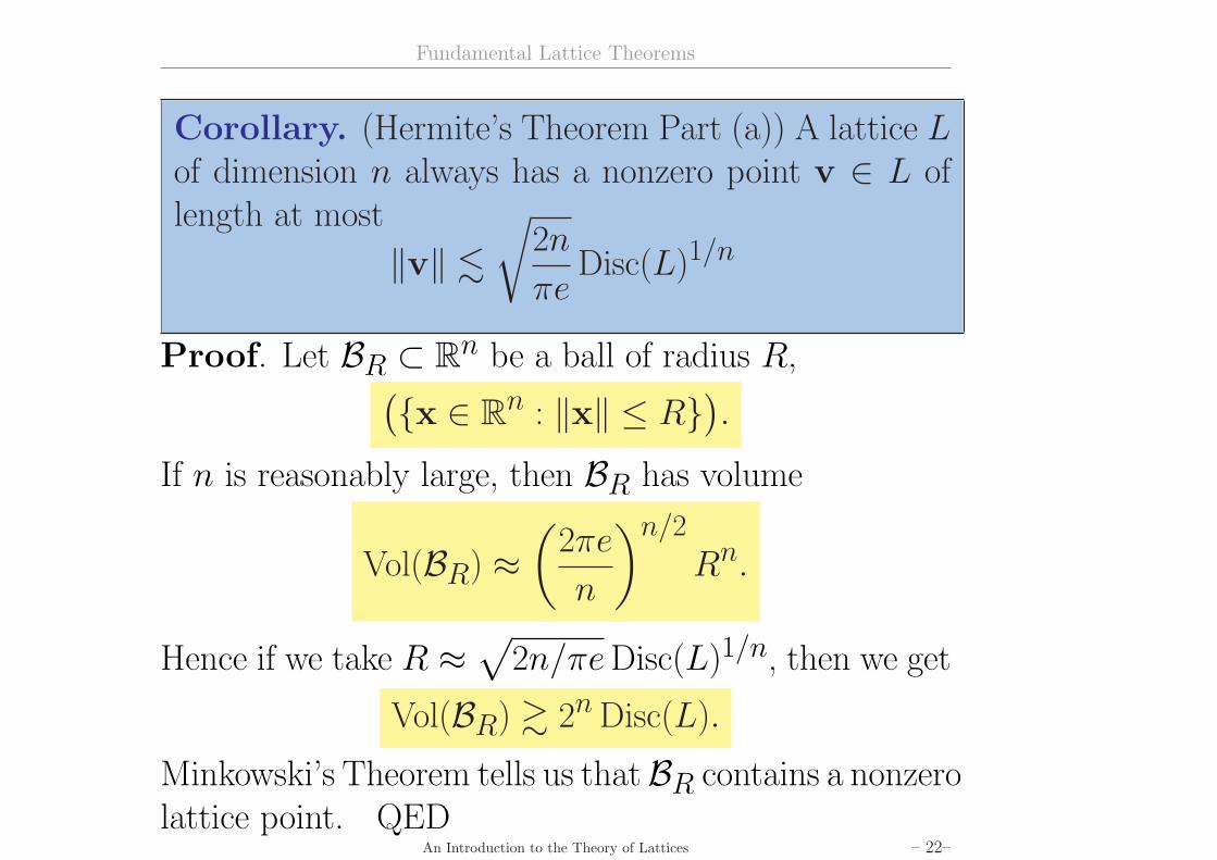
Corollary. (Hermite’s Theorem Part (a)) A lattice Lof dimension n always has a nonzero point v ∈ L oflength at most

‖v‖ .√

2n

πeDisc(L)1/n

Proof. Let BR ⊂ Rn be a ball of radius R,({x ∈ Rn : ‖x‖ ≤ R}).If n is reasonably large, then BR has volume

Vol(BR) ≈(

2πe

n

)n/2

Rn.

Hence if we take R ≈√

2n/πe Disc(L)1/n, then we get

Vol(BR) & 2n Disc(L).

Minkowski’s Theorem tells us that BR contains a nonzerolattice point. QED



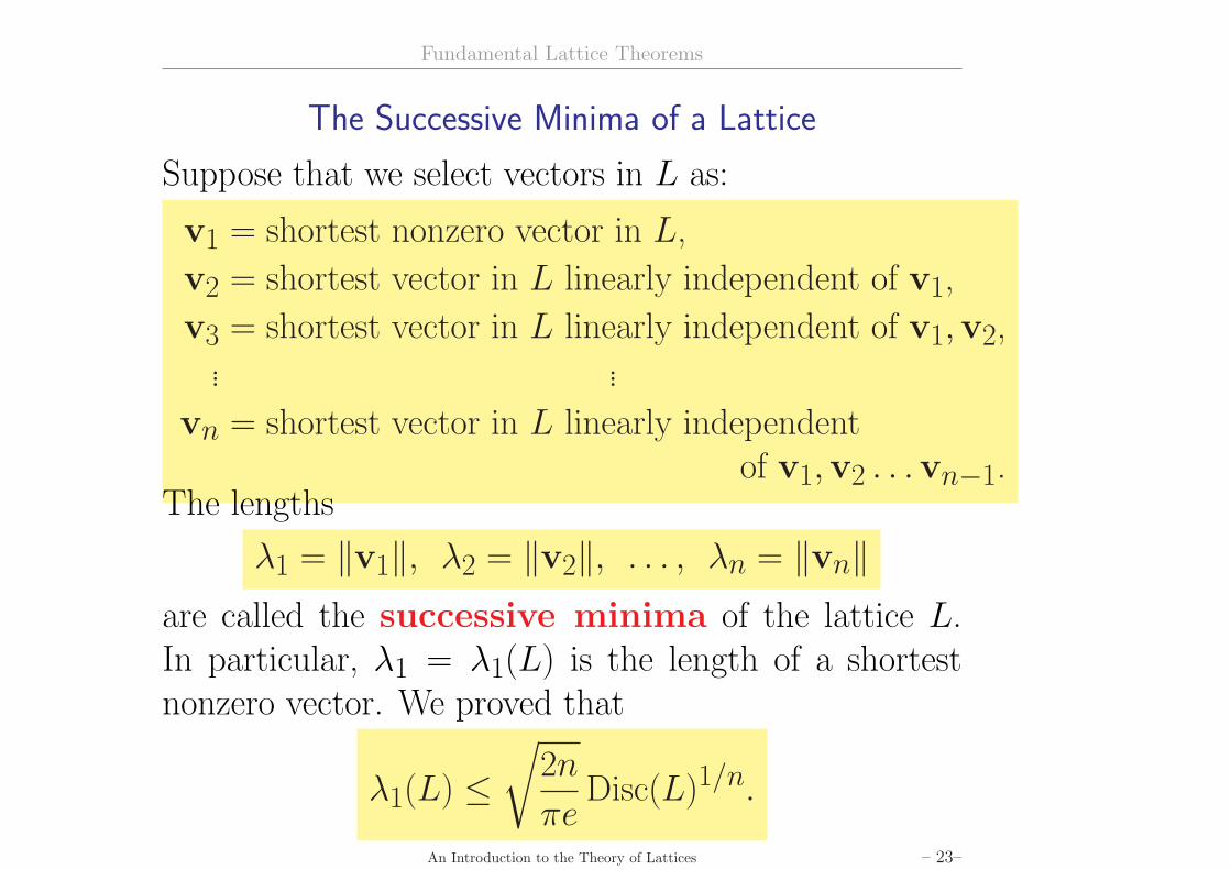
The Successive Minima of a Lattice

Suppose that we select vectors in L as:

v1 = shortest nonzero vector in L,

v2 = shortest vector in L linearly independent of v1,

v3 = shortest vector in L linearly independent of v1,v2,... ...

vn = shortest vector in L linearly independentof v1,v2 . . .vn−1.

The lengths

λ1 = ‖v1‖, λ2 = ‖v2‖, . . . , λn = ‖vn‖are called the successive minima of the lattice L.In particular, λ1 = λ1(L) is the length of a shortestnonzero vector. We proved that

λ1(L) ≤√

2n

πeDisc(L)1/n.


Lattice Reductionand the

LLL Algorithm

Lattice Reduction and the LLL Algorithm

Solving SVP and CVP in Practice

• The shortest vector problem (SVP) and the closestvector problems (CVP) are clearly closely related.In practice, CVP seems slightly harder than SVP.

• If the dimension of the lattice L is large, both SVPand CVP are very difficult to solve.

• In full generality, CVP is known to be NP-hardand SVP is NP-hard under a randomized reductionhypothesis.

• Lattice Reduction is the name given to thepractical problem of solving SVP and CVP, or moregenerally of finding reasonably short vectors andreasonably good bases.



Algorithms to (Approximately) Solve SVP

• The best lattice reduction methods currently knownare based on the LLL Algorithm of Lenstra,Lenstra, and Lovasz, orginally described in Math-ematische Annalen 261 (1982), 515-534

• LLL finds moderately short lattice vectors in poly-nomial time. This suffices for many applications.

• However, finding very short (or very close) vectorsis currently still exponentially hard.

• It is worth noting that current lattice reduction al-gorithms such as LLL are highly sequential. Thusthey are not distributable (although somewhat par-allelizable). Further, there are no quantum algo-rithms known to solve SVP or CVP.



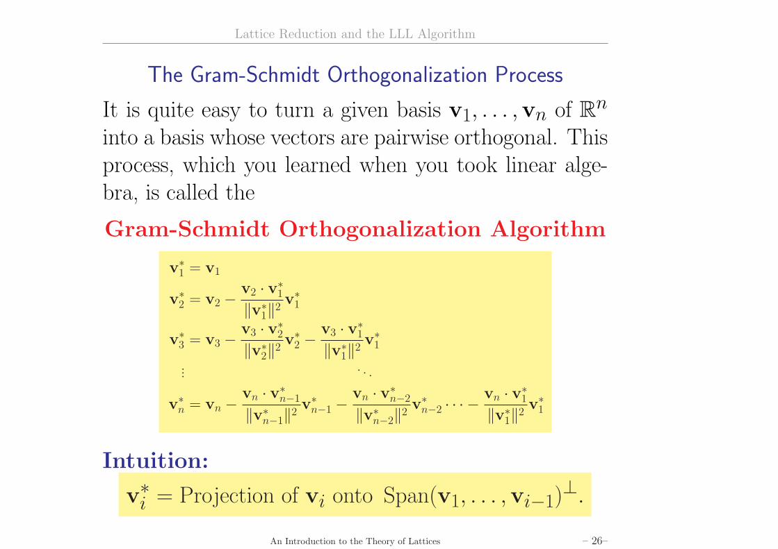
The Gram-Schmidt Orthogonalization Process

It is quite easy to turn a given basis v1, . . . ,vn of Rn

into a basis whose vectors are pairwise orthogonal. Thisprocess, which you learned when you took linear alge-bra, is called the

Gram-Schmidt Orthogonalization Algorithm

v∗1 = v1

v∗2 = v2 − v2 · v∗1‖v∗1‖2

v∗1

v∗3 = v3 − v3 · v∗2‖v∗2‖2

v∗2 −v3 · v∗1‖v∗1‖2

v∗1... . . .

v∗n = vn − vn · v∗n−1

‖v∗n−1‖2v∗n−1 −

vn · v∗n−2

‖v∗n−2‖2v∗n−2 · · · −

vn · v∗1‖v∗1‖2

v∗1

Intuition:

v∗i = Projection of vi onto Span(v1, . . . ,vi−1)⊥.



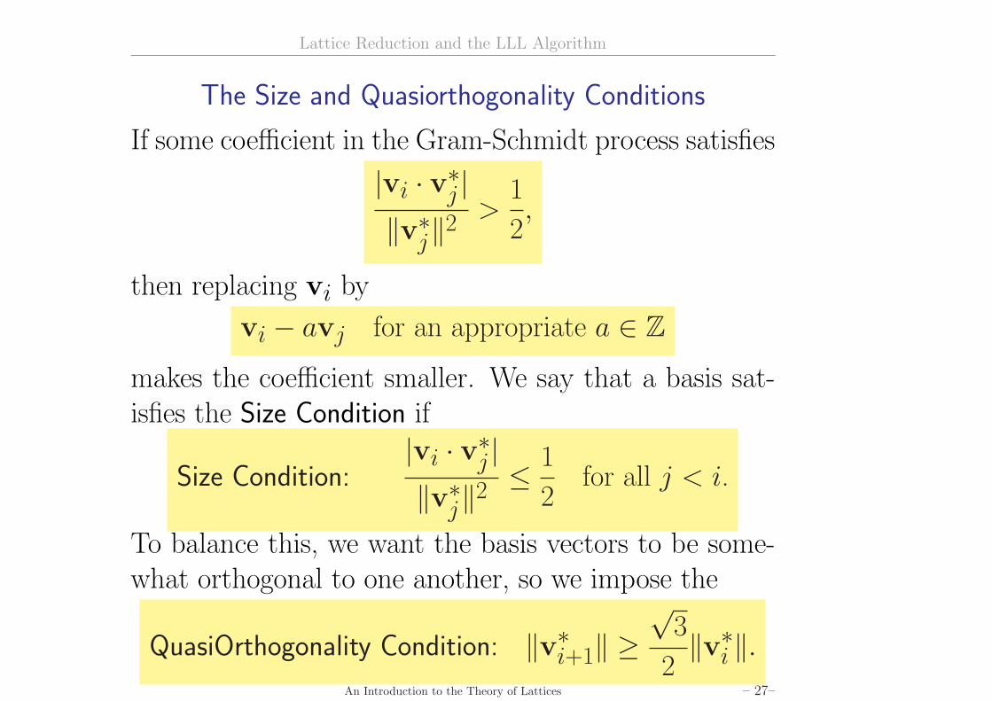
The Size and Quasiorthogonality Conditions

If some coefficient in the Gram-Schmidt process satisfies

|vi · v∗j |‖v∗j‖2

>1

2,

then replacing vi by

vi − avj for an appropriate a ∈ Zmakes the coefficient smaller. We say that a basis sat-isfies the Size Condition if

Size Condition:|vi · v∗j |‖v∗j‖2

≤ 1

2for all j < i.

To balance this, we want the basis vectors to be some-what orthogonal to one another, so we impose the

QuasiOrthogonality Condition: ‖v∗i+1‖ ≥√

3

2‖v∗i ‖.



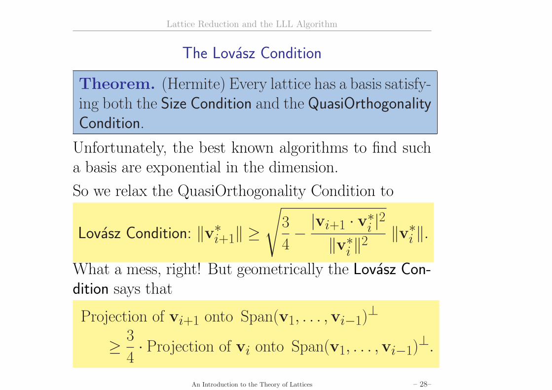
The Lovasz Condition

Theorem. (Hermite) Every lattice has a basis satisfy-ing both the Size Condition and the QuasiOrthogonalityCondition.

Unfortunately, the best known algorithms to find sucha basis are exponential in the dimension.

So we relax the QuasiOrthogonality Condition to

Lovasz Condition: ‖v∗i+1‖ ≥√

3

4− |vi+1 · v∗i |2

‖v∗i ‖2‖v∗i ‖.

What a mess, right! But geometrically the Lovasz Con-dition says that

Projection of vi+1 onto Span(v1, . . . ,vi−1)⊥

≥ 3

4· Projection of vi onto Span(v1, . . . ,vi−1)

⊥.



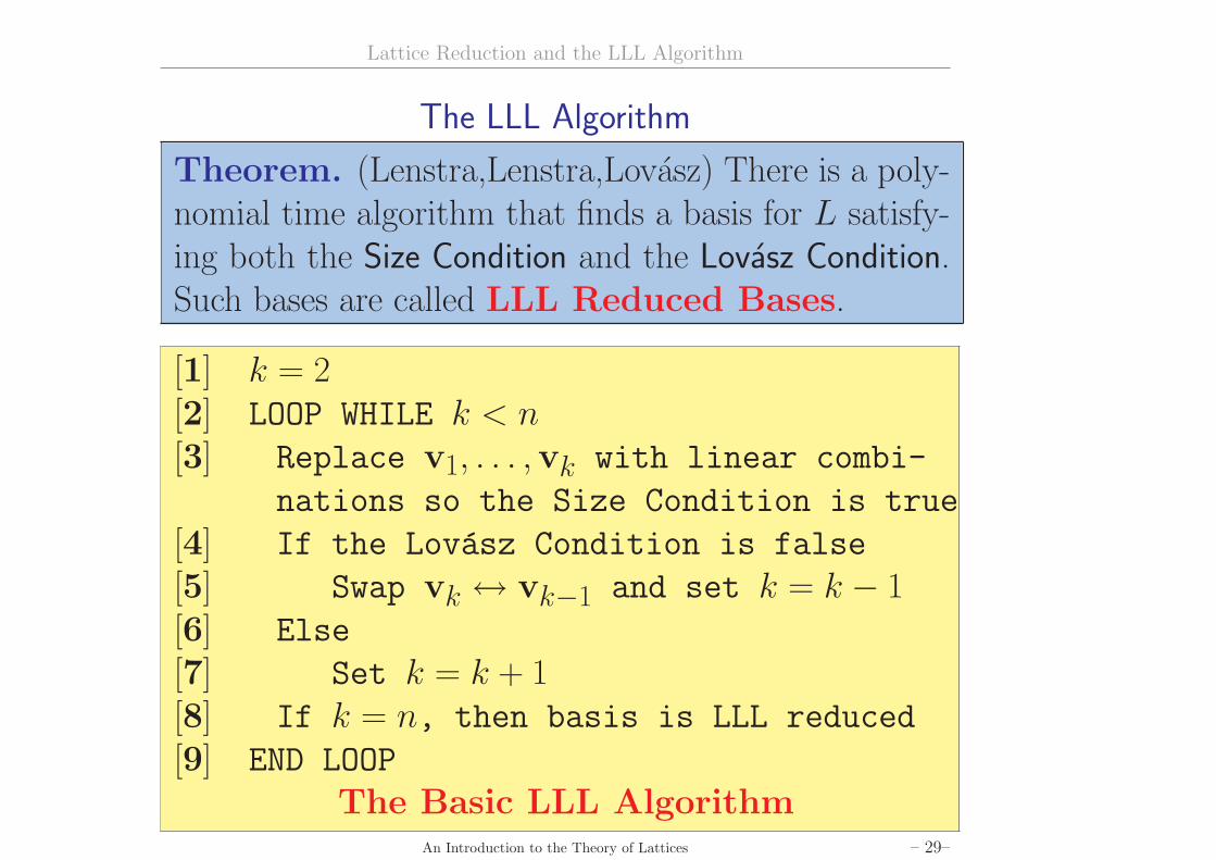
The LLL Algorithm

Theorem. (Lenstra,Lenstra,Lovasz) There is a poly-nomial time algorithm that finds a basis for L satisfy-ing both the Size Condition and the Lovasz Condition.Such bases are called LLL Reduced Bases.

[1] k = 2[2] LOOP WHILE k < n[3] Replace v1, . . . ,vk with linear combi-

nations so the Size Condition is true

[4] If the Lovasz Condition is false

[5] Swap vk ↔ vk−1 and set k = k − 1[6] Else

[7] Set k = k + 1[8] If k = n, then basis is LLL reduced

[9] END LOOP

The Basic LLL AlgorithmAn Introduction to the Theory of Lattices – 29–


Operating Characteristics of LLL

• It is clear that if k = n in Step 8, then the basis isLLL reduced.

• Step 7 helps us by incrementing k. But poten-tially there is problem because the Swapping Step(Step 5) decrements k.

• It is not hard to prove that Step 5 is executed onlyfinitely many times and the number of executionsis bounded by a polynomial in n. Thus LLL is apolynomial-time algorithm.

• The LLL algorithm is guaranteed to find a v ∈ Lsatisfying

0 < ‖v‖ ≤ 2(n−2)/2λ1(L).

• In practice, LLL generally does better than this.But also in practice, if n is large, then LLL will notfind a vector just a few times longer than λ1(L).



Variants and Improvements to LLL

Many methods of improving LLL have been proposedover the years. Often they sacrifice provable polynomialtime performance for improved operation on most lat-tices. One of the most important replaces the SwappingStep with a more complicated procedure.

Definition A KZ Reduced Basis is a basis thatsatisfies both the Size Condition and the following:

For all i, v∗i is the shortest vector in theprojection of L onto Span(v1, . . . ,vi).

Block Reduction Algorithm (BKZ-LLL).(Schnorr) Instead of swapping vk and vk−1 in Step 5of LLL, instead take the lattice spanned by a block ofvectors vi,vi+1, . . . ,vi+β−1 and replace them with aKZ Reduced Basis.



Operating Characteristics of BKZ-LLL

An advantage of BKZ-LLL is that the output improvesas one increases the block size β. Indeed, taking β = ngives a full KZ reduced basis for L, so it solves SVP.Of course, the improved output comes at a cost of in-creased running time.For a moderately large block size β, one can prove thatBKZ-LLL finds a nonzero vector v ∈ L satisfying

‖v‖ ≤(

β

πe

)n−1β−1

λ1(L).

Unfortunately, the running time of standard LLL is in-creased by a factor of (at least) Cβ for some constant C.

Experimentally one finds this borne out: For a fixed(small) constant c, the time for LLL-BKZ to find a v ∈L satisfying ‖v‖ ≤ ncλ1(L) is exponential in n.


Knapsack Cryptosystemsand

Lattice Cryptanalysis

Knapsack Cryptosystems and Lattice Cryptanalysis

The Knapsack (Subset Sum) Problem

Leta = (a1, a2, . . . , an)

be a list of positive integers.

Knapsack (Subset Sum) ProblemGiven a target integer t, determine if thereare values x1, x2, . . . , xn ∈ {0, 1} satisfying

x1a1 + x2a2 + · · · + xnan = t.

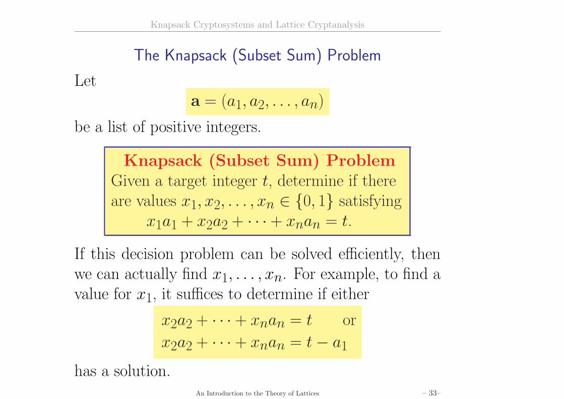
If this decision problem can be solved efficiently, thenwe can actually find x1, . . . , xn. For example, to find avalue for x1, it suffices to determine if either

x2a2 + · · · + xnan = t or

x2a2 + · · · + xnan = t− a1

has a solution.An Introduction to the Theory of Lattices – 33–


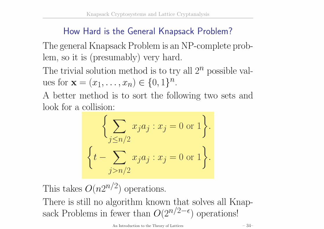
How Hard is the General Knapsack Problem?

The general Knapsack Problem is an NP-complete prob-lem, so it is (presumably) very hard.

The trivial solution method is to try all 2n possible val-ues for x = (x1, . . . , xn) ∈ {0, 1}n.

A better method is to sort the following two sets andlook for a collision:{ ∑

j≤n/2

xjaj : xj = 0 or 1

}.

{t−

∑

j>n/2

xjaj : xj = 0 or 1

}.

This takes O(n2n/2) operations.

There is still no algorithm known that solves all Knap-sack Problems in fewer than O(2n/2−ε) operations!



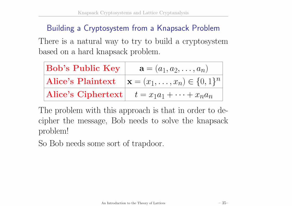
Building a Cryptosystem from a Knapsack Problem

There is a natural way to try to build a cryptosystembased on a hard knapsack problem.

Bob’s Public Key a = (a1, a2, . . . , an)

Alice’s Plaintext x = (x1, . . . , xn) ∈ {0, 1}nAlice’s Ciphertext t = x1a1 + · · · + xnan

The problem with this approach is that in order to de-cipher the message, Bob needs to solve the knapsackproblem!

So Bob needs some sort of trapdoor.




Some knapsack problems are very easy to solve.

Suppose the weights a1, . . . , an are superincreasing,

aj > a1 + a2 + · · · + aj−1 for each 1 < j ≤ n.

Then we can easily find xn, since

xn = 1 if and only if t > a1 + a2 + · · · + an−1.

Having determined xn, we are reduced to the lower di-mensional knapsack problem

x1a1 + · · · + xn−1an−1 = t− xnan,

so we can recover xn−1, . . . , x1 recursively.

Unfortunately, since a1, . . . , an are public knowledge,an attacker can deciper the message as easily as Bob.




The solution proposed by Merkle and Hellman in 1978was to conceal Bob’s private superincreasing set

a = (a1, a2, . . . , an)

by some sort of invertible transformation.

To illustrate the general method, I will describe Merkleand Hellman’s original single-transformation system andshow how it can be viewed as a lattice problem and (of-ten) solved using lattice reduction.

Merkle and Hellman and others subsequently proposedmore complicated knapsack-based cryptosystems, butas far as I am aware, all practical systems have beenbroken using lattice reduction methods.



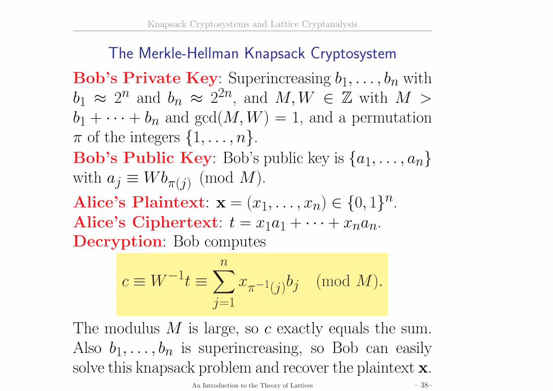
The Merkle-Hellman Knapsack Cryptosystem

Bob’s Private Key: Superincreasing b1, . . . , bn withb1 ≈ 2n and bn ≈ 22n, and M,W ∈ Z with M >b1 + · · · + bn and gcd(M,W ) = 1, and a permutationπ of the integers {1, . . . , n}.Bob’s Public Key: Bob’s public key is {a1, . . . , an}with aj ≡ Wbπ(j) (mod M).

Alice’s Plaintext: x = (x1, . . . , xn) ∈ {0, 1}n.Alice’s Ciphertext: t = x1a1 + · · · + xnan.Decryption: Bob computes

c ≡ W−1t ≡n∑

j=1

xπ−1(j)bj (mod M).

The modulus M is large, so c exactly equals the sum.Also b1, . . . , bn is superincreasing, so Bob can easilysolve this knapsack problem and recover the plaintext x.



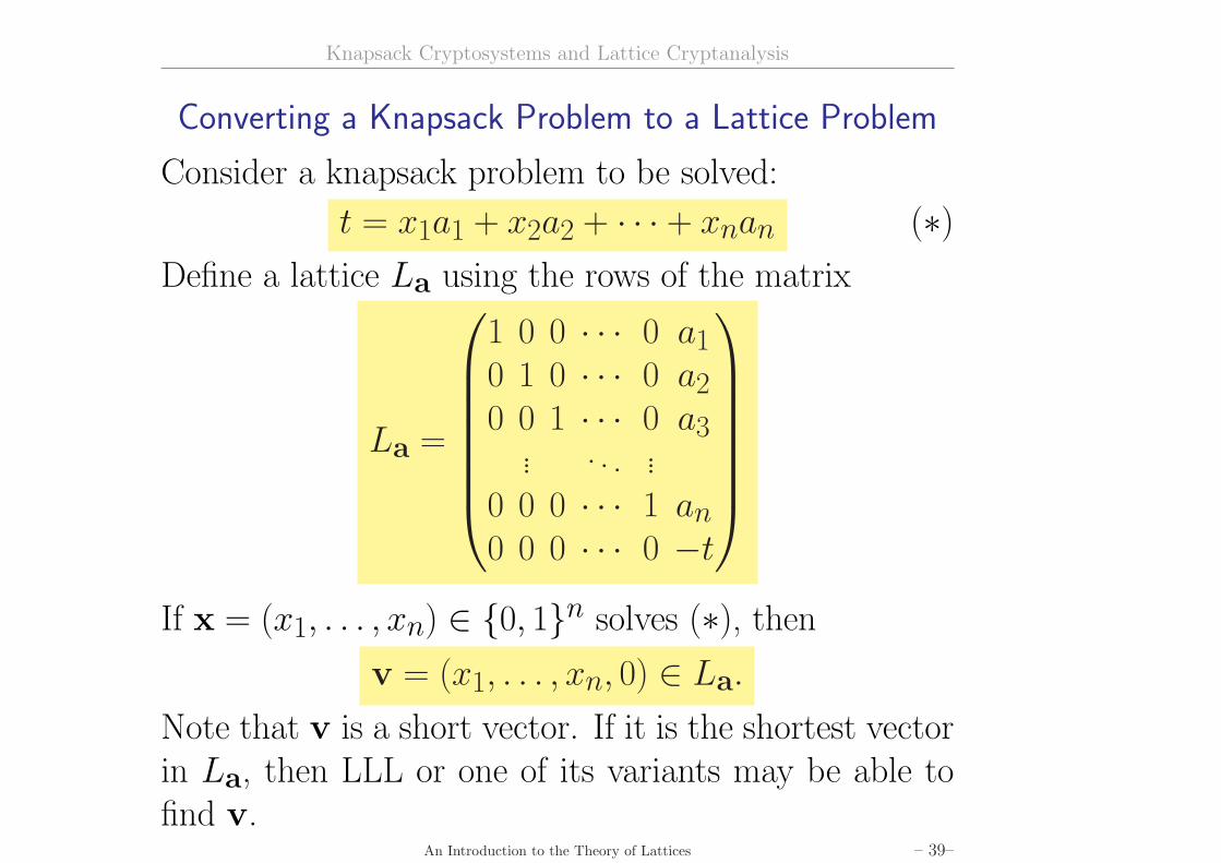
Converting a Knapsack Problem to a Lattice Problem

Consider a knapsack problem to be solved:

t = x1a1 + x2a2 + · · · + xnan (∗)Define a lattice La using the rows of the matrix

La =

1 0 0 · · · 0 a10 1 0 · · · 0 a20 0 1 · · · 0 a3

... . . . ...0 0 0 · · · 1 an

0 0 0 · · · 0 −t

If x = (x1, . . . , xn) ∈ {0, 1}n solves (∗), then

v = (x1, . . . , xn, 0) ∈ La.

Note that v is a short vector. If it is the shortest vectorin La, then LLL or one of its variants may be able tofind v.



Other Applications of Lattices to Cryptanalysis

There are many other applications of lattice reductionto cryptanalysis. For example, suppose that p and qare unknown large primes with p ≈ q and that n = pqis given. Suppose further than somehow the top-orderbits of p have been leaked. Then the attacker knowsnumbers p0 and q0 so that

x = p− p0 and y = q − q0 are “small”.

If x < n1/4 and y < n1/4, then Don Coppersmithshowed how to set up a lattice problem whose solutionwould reveal x and y.

Another example is the use of lattice reduction to breakRSA when the decryption exponent is small, or whenthe encryption exponent is small and similar messagesare transmitted. (But no general method is known forsmall encryption exponenets.)


Lattice-BasedCryptography

Lattice-Based Cryptography

Why Attempt To Use Lattices To Build Cryptosystems?

The reason that the Merkle-Hellman and other knap-sack cryptosystems attracted attention is because theyare much faster than RSA, often by a factor of 10 to 100.

For example, if N and d are n bit numbers, it takesapproximately

n3 steps to compute ad mod N .

But knapsack encrypt/decrypt take only about n2 steps.

On the other hand, it is sadly also true that slow securecryptosystems do have some “small” advantages overfast insecure cryptosystems!

However, the speed advantages available from latticeoperations combined with the fact that SVP and CVPare well-studied hard problems make it worth lookingfor other constructions whose security depends more di-rectly on SVP and CVP.



The Ajtai-Dwork Lattice Cryptosystem

• Ajtai and Dwork (1995) described a lattice-basedpublic key cryptosystem whose security relies onthe difficulty of solving CVP in certain class of lat-tices LAD.

• They proved that breaking their system in the av-erage case (i.e., for a randomly chosen lattice ofdimension m in LAD) is as difficult as solving SVPfor all lattices of dimension n (for a certain n thatdepends on m).

• This average case-worst case equivalence is a theo-retical cryptographic milestone, but unfortunatelythe Ajtai-Dwork cryptosystem is impractical.

• Inspired by the work of Ajtai and Dwork, a morepractical lattice-based cryptosystem was proposedin 1996 by Goldreich, Goldwasser, and Halevi.



The GGH Public Key Cryptosystem

Key Creation: Choose a lattice L andPrivate Key = {v1, . . . ,vn} a good (short) basis,

Public Key = {w1, . . . ,wn} a bad (long) basis.

Encryption: The plaintext m is a binary vector. Alsochoose a small random “perturbation” vector r. Theciphertext is e = m1w1 + m2w2 + · · · + mnwn + r.

Note that the ciphertext vector e is not in the lattice L.

Decryption: Find a vector u in L that is closest to e.If r is small enough, then u = m1w1 + · · · + mnwn,so solving CVP for e in L will recover m. The privategood basis can be used to find u. First write

e = µ1v1 + · · · + µnvn using real µ1, . . . , µn ∈ R.

Then round µ1, . . . , µn to the nearest integer:

bµ1ev1 + · · · + bµnevn will equal u.An Introduction to the Theory of Lattices – 43–


GGH versus LLL: A Lesson in Practicality

The security of GGH rests on the difficulty of solvingCVP using a highly nonorthogonal basis.The LLL lattice reduction algorithm finds a moder-ately orthogonal basis in polynomial time.

In practice, if n = dim(L) < 100, then LLL easily findsa good enough basis to break GGH. Even for n < 200,variants of LLL give a practical way to break GGH.

The public key for GGH is a basis for L, so

Size of GGH Public Key = O(n2) bits.

GGH is currently secure for (say) n = 500, but 2 megabitkeys are impractical!The NTRU Public Key Cryptosystem solves this prob-lem by using a type of lattice whose bases can be de-

scribed using only 12n log2(n) bits.


NTRUEncrypt: The NTRUPublic Key Cryptosystem

NTRUEncrypt: The NTRU Public Key Cryptosystem

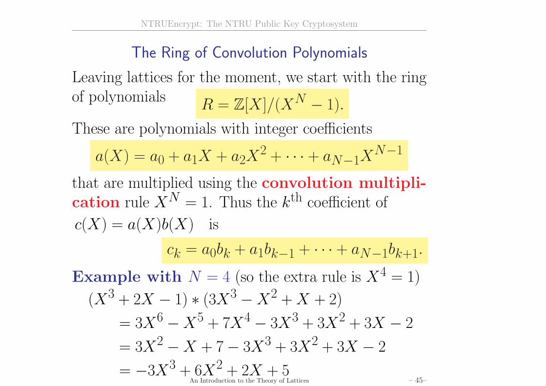
The Ring of Convolution Polynomials

Leaving lattices for the moment, we start with the ringof polynomials R = Z[X ]/(XN − 1).

These are polynomials with integer coefficients

a(X) = a0 + a1X + a2X2 + · · · + aN−1X

N−1

that are multiplied using the convolution multipli-cation rule XN = 1. Thus the kth coefficient of

c(X) = a(X)b(X) is

ck = a0bk + a1bk−1 + · · · + aN−1bk+1.

Example with N = 4 (so the extra rule is X4 = 1)

(X3 + 2X − 1) ∗ (3X3 −X2 + X + 2)

= 3X6 −X5 + 7X4 − 3X3 + 3X2 + 3X − 2

= 3X2 −X + 7− 3X3 + 3X2 + 3X − 2

= −3X3 + 6X2 + 2X + 5An Introduction to the Theory of Lattices – 45–


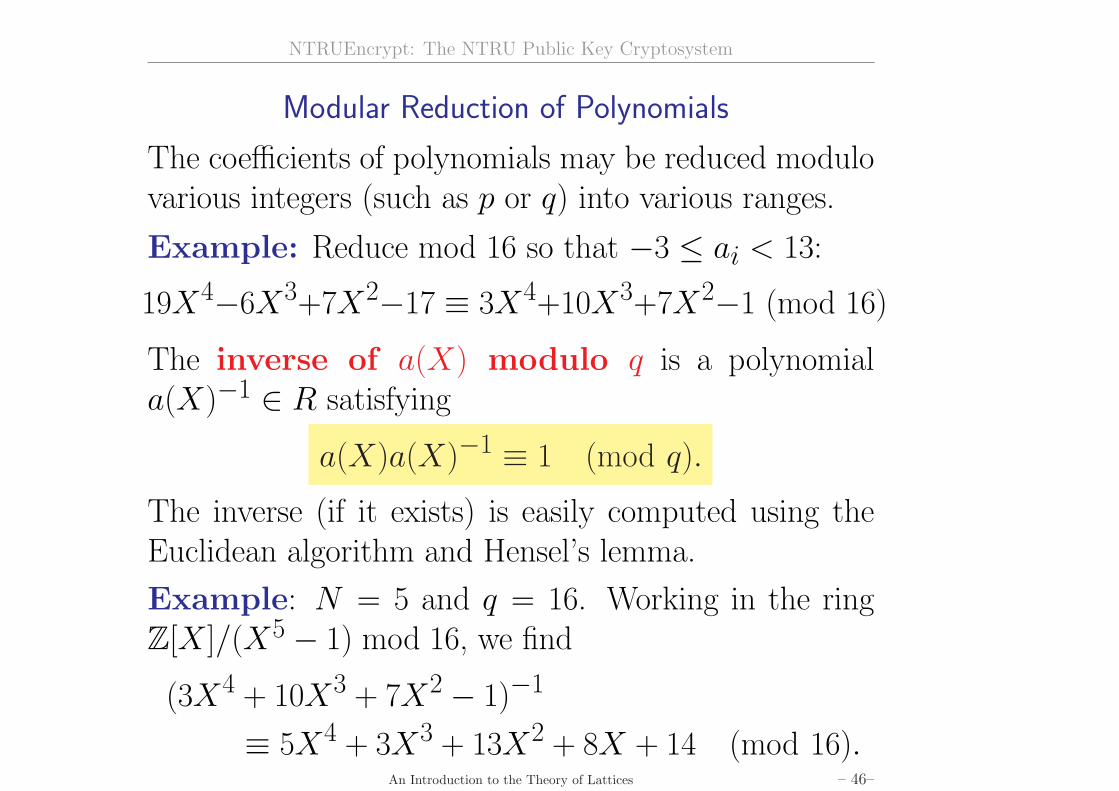
Modular Reduction of Polynomials

The coefficients of polynomials may be reduced modulovarious integers (such as p or q) into various ranges.

Example: Reduce mod 16 so that −3 ≤ ai < 13:

19X4−6X3+7X2−17 ≡ 3X4+10X3+7X2−1 (mod 16)

The inverse of a(X) modulo q is a polynomiala(X)−1 ∈ R satisfying

a(X)a(X)−1 ≡ 1 (mod q).

The inverse (if it exists) is easily computed using theEuclidean algorithm and Hensel’s lemma.

Example: N = 5 and q = 16. Working in the ringZ[X ]/(X5 − 1) mod 16, we find

(3X4 + 10X3 + 7X2 − 1)−1

≡ 5X4 + 3X3 + 13X2 + 8X + 14 (mod 16).An Introduction to the Theory of Lattices – 46–


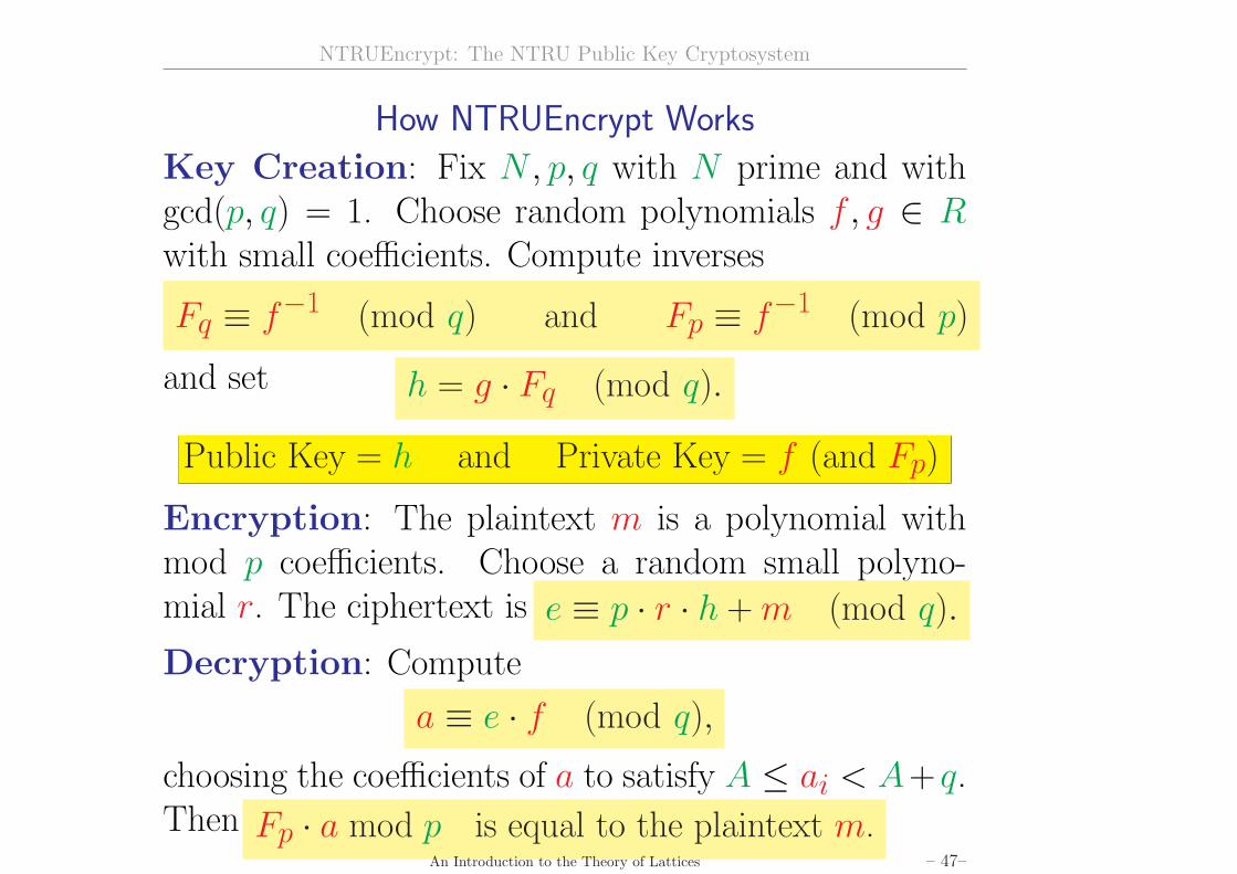
How NTRUEncrypt Works

Key Creation: Fix N, p, q with N prime and withgcd(p, q) = 1. Choose random polynomials f, g ∈ Rwith small coefficients. Compute inverses

Fq ≡ f−1 (mod q) and Fp ≡ f−1 (mod p)

and set h = g · Fq (mod q).

Public Key = h and Private Key = f (and Fp)

Encryption: The plaintext m is a polynomial withmod p coefficients. Choose a random small polyno-mial r. The ciphertext is e ≡ p · r · h + m (mod q).

Decryption: Compute

a ≡ e · f (mod q),

choosing the coefficients of a to satisfy A ≤ ai < A+ q.Then Fp · a mod p is equal to the plaintext m.



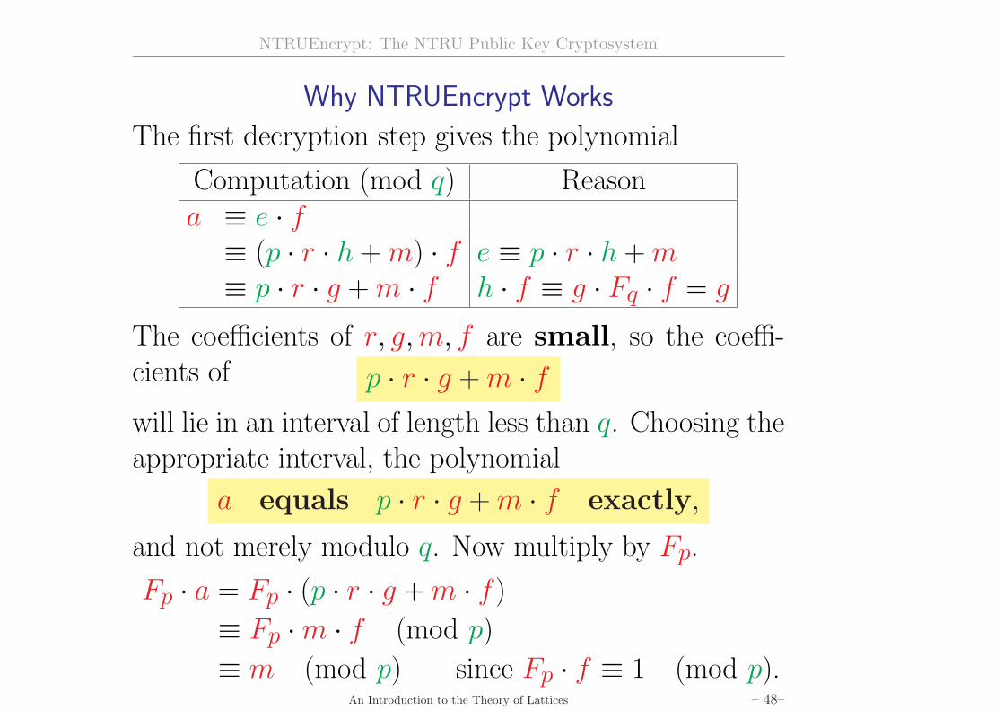
Why NTRUEncrypt Works

The first decryption step gives the polynomial

Computation (mod q) Reasona ≡ e · f≡ (p · r · h + m) · f e ≡ p · r · h + m≡ p · r · g + m · f h · f ≡ g · Fq · f = g

The coefficients of r, g, m, f are small, so the coeffi-cients of p · r · g + m · fwill lie in an interval of length less than q. Choosing theappropriate interval, the polynomial

a equals p · r · g + m · f exactly,

and not merely modulo q. Now multiply by Fp.

Fp · a = Fp · (p · r · g + m · f )

≡ Fp ·m · f (mod p)

≡ m (mod p) since Fp · f ≡ 1 (mod p).An Introduction to the Theory of Lattices – 48–


Comparison of Operating Characteristics

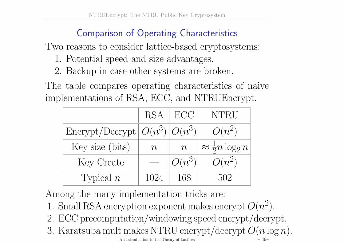
Two reasons to consider lattice-based cryptosystems:1. Potential speed and size advantages.2. Backup in case other systems are broken.

The table compares operating characteristics of naiveimplementations of RSA, ECC, and NTRUEncrypt.

RSA ECC NTRU

Encrypt/Decrypt O(n3) O(n3) O(n2)

Key size (bits) n n ≈ 12n log2 n

Key Create — O(n3) O(n2)

Typical n 1024 168 502

Among the many implementation tricks are:1. Small RSA encryption exponent makes encrypt O(n2).2. ECC precomputation/windowing speed encrypt/decrypt.3. Karatsuba mult makes NTRU encrypt/decrypt O(n log n).



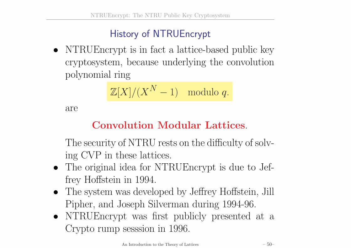
History of NTRUEncrypt

• NTRUEncrypt is in fact a lattice-based public keycryptosystem, because underlying the convolutionpolynomial ring

Z[X ]/(XN − 1) modulo q.

are

Convolution Modular Lattices.

The security of NTRU rests on the difficulty of solv-ing CVP in these lattices.

• The original idea for NTRUEncrypt is due to Jef-frey Hoffstein in 1994.

• The system was developed by Jeffrey Hoffstein, JillPipher, and Joseph Silverman during 1994-96.

• NTRUEncrypt was first publicly presented at aCrypto rump sesssion in 1996.


Convolution Modular Latticesand NTRU Lattices

Convolution Modular Lattices and NTRU Lattices

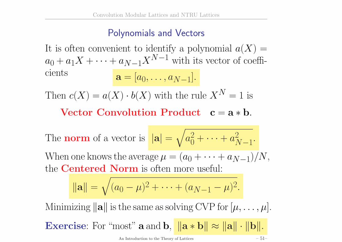
Polynomials and Vectors

It is often convenient to identify a polynomial a(X) =a0 + a1X + · · ·+ aN−1X

N−1 with its vector of coeffi-cients a = [a0, . . . , aN−1].

Then c(X) = a(X) · b(X) with the rule XN = 1 is

Vector Convolution Product c = a ∗ b.

The norm of a vector is |a| =√

a20 + · · · + a2

N−1.

When one knows the average µ = (a0 + · · · + aN−1)/N ,the Centered Norm is often more useful:

‖a‖ =√

(a0 − µ)2 + · · · + (aN−1 − µ)2.

Minimizing ‖a‖ is the same as solving CVP for [µ, . . . , µ].

Exercise: For “most” a and b, ‖a ∗ b‖ ≈ ‖a‖ · ‖b‖.An Introduction to the Theory of Lattices – 51–


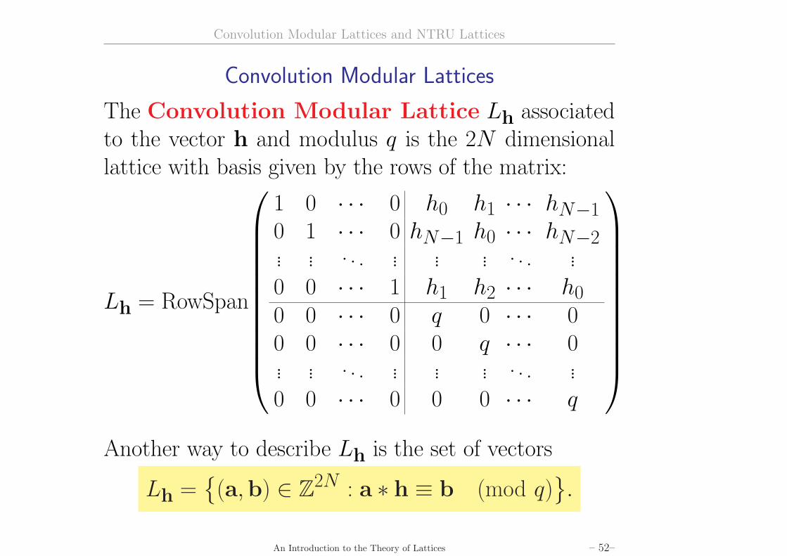
Convolution Modular Lattices

The Convolution Modular Lattice Lh associatedto the vector h and modulus q is the 2N dimensionallattice with basis given by the rows of the matrix:

Lh = RowSpan

1 0 · · · 0 h0 h1 · · · hN−10 1 · · · 0 hN−1 h0 · · · hN−2... ... . . . ... ... ... . . . ...0 0 · · · 1 h1 h2 · · · h00 0 · · · 0 q 0 · · · 00 0 · · · 0 0 q · · · 0... ... . . . ... ... ... . . . ...0 0 · · · 0 0 0 · · · q

Another way to describe Lh is the set of vectors

Lh ={(a,b) ∈ Z2N : a ∗ h ≡ b (mod q)

}.



Small Vectors in NTRU Convolution Modular Lattices

In an NTRU Convolution Modular Lattice,

f (X) · h(X) ≡ g(X) (mod q) with “small” f and g.

This convolution relation implies that the NTRU lat-tice Lh contains the short vector

[f ,g] = [f0, f1, . . . , fN−1, g0, g1, . . . , gN−1].

To see that [f ,g] is in Lh, let

u(X) =−f (X) · h(X) + g(X)

q∈ Z[X ].

Then

[f0, . . . , fN−1, u0, . . . , uN−1]

1 · · · 0 h0 · · · hN−1... . . . ... ... . . . ...

0 · · · 1 h1 · · · h0

0 · · · 0 q · · · 0... . . . ... ... . . . ...

0 · · · 0 0 · · · q

= [f0, . . . , fN−1, g0, . . . , gN−1].



Convolution Modular Lattices as R-Modules

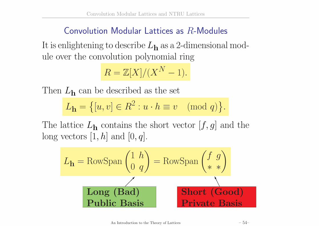
It is enlightening to describe Lh as a 2-dimensional mod-ule over the convolution polynomial ring

R = Z[X ]/(XN − 1).

Then Lh can be described as the set

Lh ={[u, v] ∈ R2 : u · h ≡ v (mod q)

}.

The lattice Lh contains the short vector [f, g] and thelong vectors [1, h] and [0, q].

Lh = RowSpan

(1 h0 q

)= RowSpan

(f g∗ ∗

)

Long (Bad)Public Basis

¡¡¡µ

Short (Good)Private Basis

AAAK



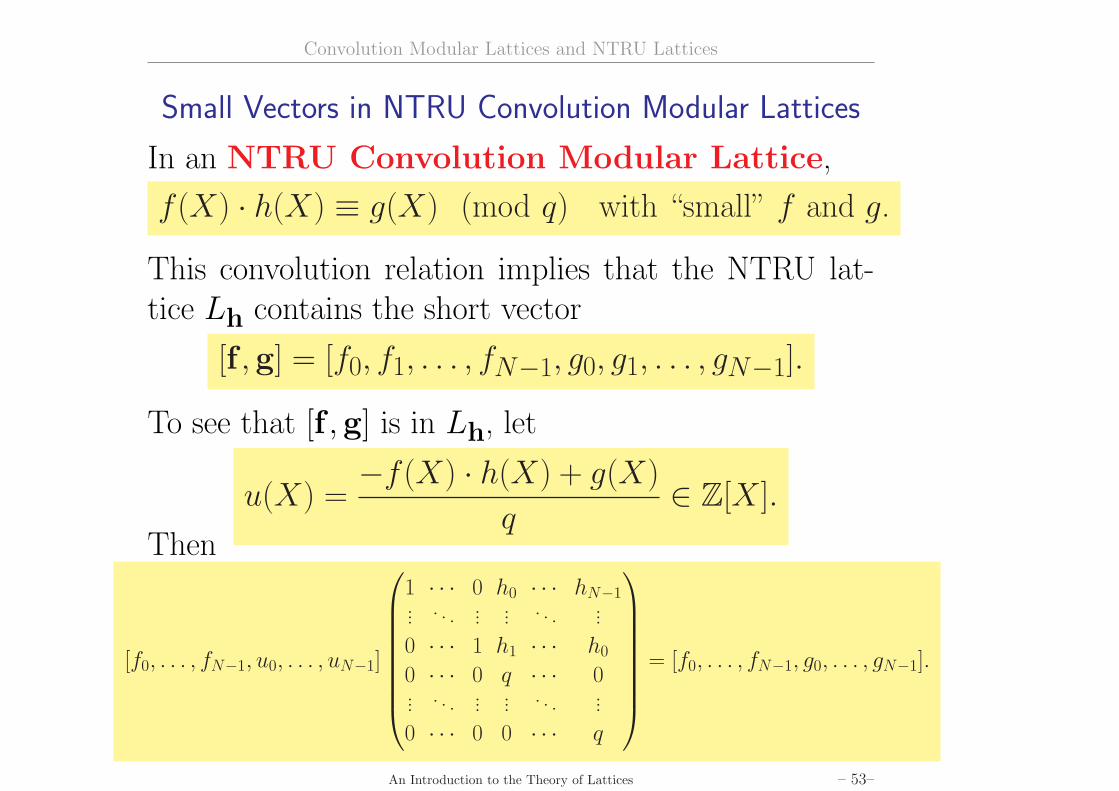
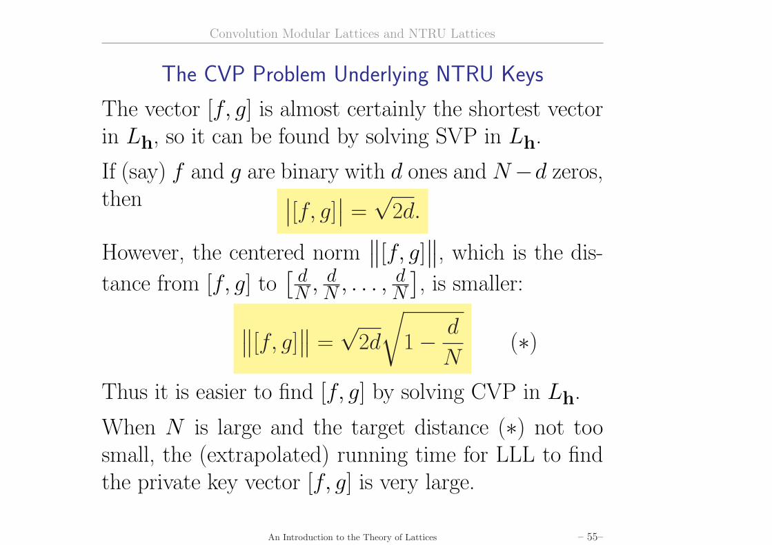
The CVP Problem Underlying NTRU Keys

The vector [f, g] is almost certainly the shortest vectorin Lh, so it can be found by solving SVP in Lh.

If (say) f and g are binary with d ones and N−d zeros,then ∣∣[f, g]

∣∣ =√

2d.

However, the centered norm∥∥[f, g]

∥∥, which is the dis-

tance from [f, g] to[ dN , d

N , . . . , dN

], is smaller:

∥∥[f, g]∥∥ =

√2d

√1− d

N(∗)

Thus it is easier to find [f, g] by solving CVP in Lh.

When N is large and the target distance (∗) not toosmall, the (extrapolated) running time for LLL to findthe private key vector [f, g] is very large.



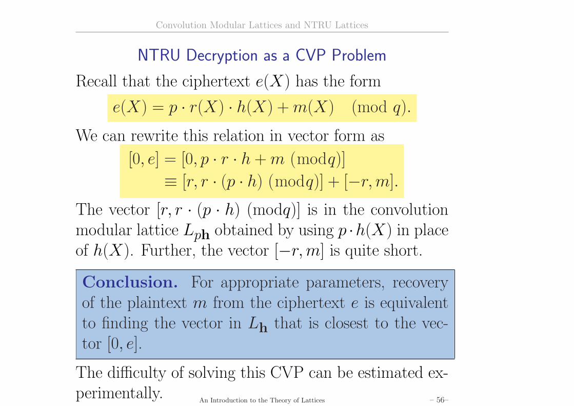
NTRU Decryption as a CVP Problem

Recall that the ciphertext e(X) has the form

e(X) = p · r(X) · h(X) + m(X) (mod q).

We can rewrite this relation in vector form as

[0, e] = [0, p · r · h + m (modq)]

≡ [r, r · (p · h) (modq)] + [−r,m].

The vector [r, r · (p · h) (modq)] is in the convolutionmodular lattice Lph obtained by using p ·h(X) in placeof h(X). Further, the vector [−r,m] is quite short.

Conclusion. For appropriate parameters, recoveryof the plaintext m from the ciphertext e is equivalentto finding the vector in Lh that is closest to the vec-tor [0, e].

The difficulty of solving this CVP can be estimated ex-perimentally.



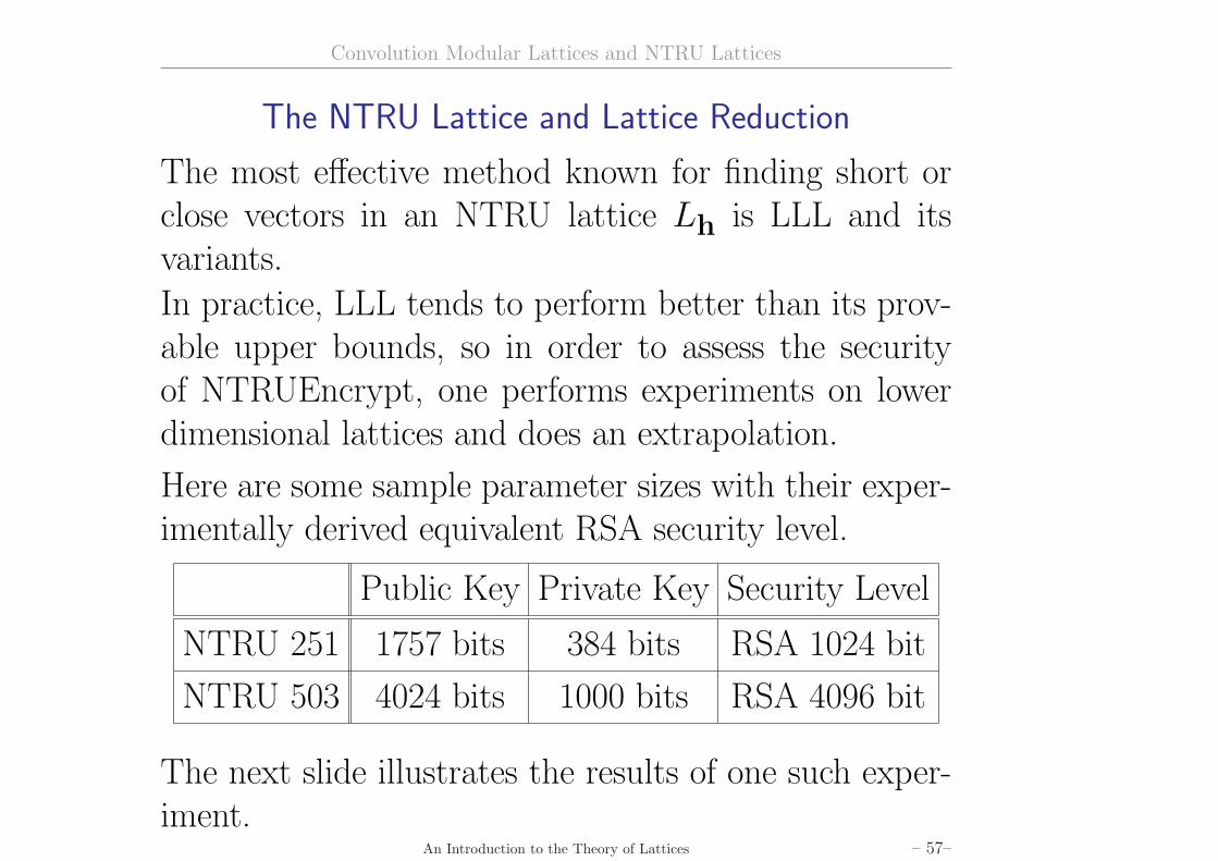
The NTRU Lattice and Lattice Reduction

The most effective method known for finding short orclose vectors in an NTRU lattice Lh is LLL and itsvariants.

In practice, LLL tends to perform better than its prov-able upper bounds, so in order to assess the securityof NTRUEncrypt, one performs experiments on lowerdimensional lattices and does an extrapolation.

Here are some sample parameter sizes with their exper-imentally derived equivalent RSA security level.

Public Key Private Key Security Level

NTRU 251 1757 bits 384 bits RSA 1024 bit

NTRU 503 4024 bits 1000 bits RSA 4096 bit

The next slide illustrates the results of one such exper-iment.



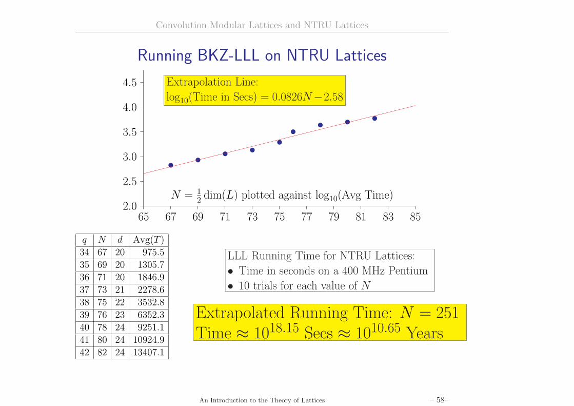
Running BKZ-LLL on NTRU Lattices

65 67 69 71 73 75 77 79 81 83 852.0

2.5

3.0

3.5

4.0

4.5

v vv v

vv

v v v

»»»»»»»»»»»»»»»»»»»»»»»»»»»»»»»»»»»»»»»»

Extrapolation Line:

log10(Time in Secs) = 0.0826N−2.58

N = 12 dim(L) plotted against log10(Avg Time)

q N d Avg(T )

34 67 20 975.5

35 69 20 1305.7

36 71 20 1846.9

37 73 21 2278.6

38 75 22 3532.8

39 76 23 6352.3

40 78 24 9251.1

41 80 24 10924.9

42 82 24 13407.1

LLL Running Time for NTRU Lattices:

• Time in seconds on a 400 MHz Pentium

• 10 trials for each value of N

Extrapolated Running Time: N = 251Time ≈ 1018.15 Secs ≈ 1010.65 Years


Random Latticesand the

Gaussian Heuristic

Random Lattices and the Gaussian Heuristic

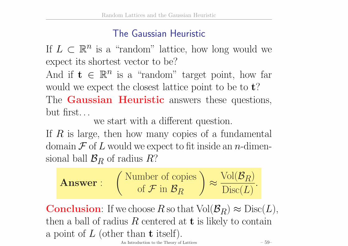
The Gaussian Heuristic

If L ⊂ Rn is a “random” lattice, how long would weexpect its shortest vector to be?

And if t ∈ Rn is a “random” target point, how farwould we expect the closest lattice point to be to t?The Gaussian Heuristic answers these questions,but first. . .

we start with a different question.

If R is large, then how many copies of a fundamentaldomainF of L would we expect to fit inside an n-dimen-sional ball BR of radius R?

Answer :

(Number of copies

of F in BR

)≈ Vol(BR)

Disc(L).

Conclusion: If we choose R so that Vol(BR) ≈ Disc(L),then a ball of radius R centered at t is likely to containa point of L (other than t itself).



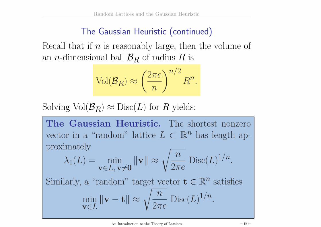
The Gaussian Heuristic (continued)

Recall that if n is reasonably large, then the volume ofan n-dimensional ball BR of radius R is

Vol(BR) ≈(

2πe

n

)n/2

Rn.

Solving Vol(BR) ≈ Disc(L) for R yields:

The Gaussian Heuristic. The shortest nonzerovector in a “random” lattice L ⊂ Rn has length ap-proximately

λ1(L) = minv∈L,v 6=0

‖v‖ ≈√

n

2πeDisc(L)1/n.

Similarly, a “random” target vector t ∈ Rn satisfies

minv∈L

‖v − t‖ ≈√

n

2πeDisc(L)1/n.



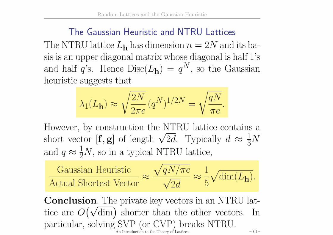
The Gaussian Heuristic and NTRU Lattices

The NTRU lattice Lh has dimension n = 2N and its ba-sis is an upper diagonal matrix whose diagonal is half 1’sand half q’s. Hence Disc(Lh) = qN , so the Gaussianheuristic suggests that

λ1(Lh) ≈√

2N

2πe(qN )1/2N =

√qN

πe.

However, by construction the NTRU lattice contains ashort vector [f ,g] of length

√2d. Typically d ≈ 1

3N

and q ≈ 12N , so in a typical NTRU lattice,

Gaussian Heuristic

Actual Shortest Vector≈

√qN/πe√

2d≈ 1

5

√dim(Lh).

Conclusion. The private key vectors in an NTRU lat-tice are O

(√dim

)shorter than the other vectors. In

particular, solving SVP (or CVP) breaks NTRU.An Introduction to the Theory of Lattices – 61–


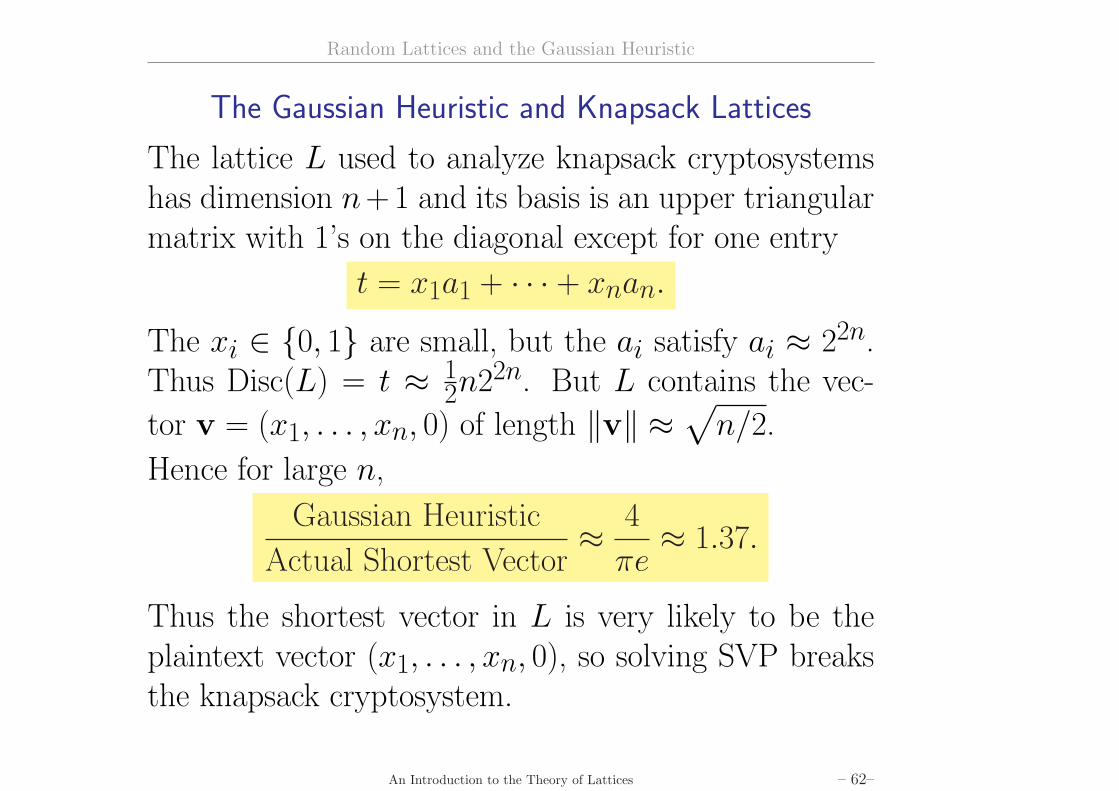
The Gaussian Heuristic and Knapsack Lattices

The lattice L used to analyze knapsack cryptosystemshas dimension n+1 and its basis is an upper triangularmatrix with 1’s on the diagonal except for one entry

t = x1a1 + · · · + xnan.

The xi ∈ {0, 1} are small, but the ai satisfy ai ≈ 22n.Thus Disc(L) = t ≈ 1

2n22n. But L contains the vec-

tor v = (x1, . . . , xn, 0) of length ‖v‖ ≈√

n/2.

Hence for large n,

Gaussian Heuristic

Actual Shortest Vector≈ 4

πe≈ 1.37.

Thus the shortest vector in L is very likely to be theplaintext vector (x1, . . . , xn, 0), so solving SVP breaksthe knapsack cryptosystem.


Some Further Remarks

Some Further Remarks

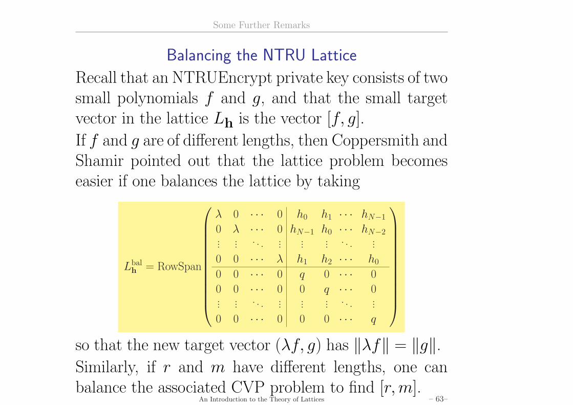
Balancing the NTRU Lattice

Recall that an NTRUEncrypt private key consists of twosmall polynomials f and g, and that the small targetvector in the lattice Lh is the vector [f, g].

If f and g are of different lengths, then Coppersmith andShamir pointed out that the lattice problem becomeseasier if one balances the lattice by taking

Lbalh = RowSpan

λ 0 · · · 0 h0 h1 · · · hN−1

0 λ · · · 0 hN−1 h0 · · · hN−2... ... . . . ... ... ... . . . ...

0 0 · · · λ h1 h2 · · · h0

0 0 · · · 0 q 0 · · · 0

0 0 · · · 0 0 q · · · 0... ... . . . ... ... ... . . . ...

0 0 · · · 0 0 0 · · · q

so that the new target vector (λf, g) has ‖λf‖ = ‖g‖.Similarly, if r and m have different lengths, one canbalance the associated CVP problem to find [r,m].


Further Reading

Further Reading

Further Reading• Ajtai, M., Dwork, C., A public-key cryptosystem with worst-case/average-

case equivalence. STOC ’97 (El Paso, TX), 284-293 ACM, New York, 1999.

[A fundamental theoretical advance in lattice-based cryptography.]

• Buchmann, J., Ludwig, C. , Practical Lattice Basis Sampling Reduction,

Cryptology ePrint Archive, Report 2005/072, http://eprint.iacr.org/.

[An improved lattice reduction method using random sampling.]

• Cryptography and Lattices Conference (CaLC), Providence, RI, Lecture

Notes in Comput. Sci. 2146, Springer, 2001. [A conference devoted to the

uses of lattices in cryptography, with may interesting articles.]

• Cassels, J. W. S. An introduction to the geometry of numbers. Classics in

Mathematics. Springer-Verlag, Berlin, 1997. [An excellent introduction.]

• Coppersmith, D., Shamir, A., Lattice attacks on NTRU. Advances in crypto-

logy-EUROCRYPT ’97, 52-61, Lect. Notes in Comput. Sci., 1233, Springer,

Berlin, 1997. [The first paper containing an analysis of NTRU.]

• Goldreich, O., Goldwasser, S., Halevi, S., Public-key cryptosystems from

lattice reduction problems. Advances in cryptology-CRYPTO ’97, 112-131,

Lecture Notes in Comput. Sci., 1294, Springer, Berlin, 1997. [Lattice-based

public key cryptosystem and digital signature scheme.]

• Gruber, P. M.; Lekkerkerker, C. G. Geometry of numbers. North-Holland

Mathematical Library, 37. North-Holland Publishing Co., Amsterdam,

1987. [The ”bible” of the subject, comprehensive and dense.]


Further Reading

Further Reading• Hoffstein, J, Pipher, J, Silverman, J.H., NTRU: A ring-based public key

cryptosystem. Algorithmic number theory (Portland, OR, 1998), 267-288,

Lecture Notes in Comput. Sci., 1423, Springer, Berlin, 1998. [The original

article describing the NTRU lattice-based cryptosystem.]

• Lenstra, A., Lenstra, H., Lovasz, L., Factoring polynomials with rational

coefficients, Mathematische Ann. 261 (1982), 513-534. [The famous LLL

algorithm.]

• Nguyen, P., Stern, J., The two faces of lattices in cryptography. Cryptogra-

phy and lattices-CaLC 2001, 146-180, Lecture Notes in Comput. Sci., 2146,

Springer, Berlin, 2001. [Survey of how lattices are used both to create and

to break cryptosystems.]

• NTRU tutorials and technical notes <www.ntru.com>. [NTRU Cryptosys-

tems markets NTRU lattice-based cryptographic products.]

• Odlyzko, A. The rise and fall of knapsack cryptosystems. Cryptology and

computational number theory (Boulder, CO, 1989), 75-88, Proc. Sympos.

Appl. Math., 42, Amer. Math. Soc., 1990. [The title says it all!]

• Schnorr, C., A hierarchy of polynomial time lattice basis reduction algo-

rithms. Theoretical Computer Science 53 (1987), 201-224. [One of many ar-

ticles by Schnorr and colleagues giving improvements to the LLL algroithm.]

• Siegel, C.L., Lectures on the geometry of numbers. Springer-Verlag, Berlin,

1989. [Another excellent introduction to the subject.]


Date post:	11-Jul-2018
Category:	Documents
Upload:	dangdung
View:	216 times
Download:	0 times

An Introduction to the Theory of Lattices and …jhs/Presentations/WyomingLattices.pdfTheory of...

Documents