125
Analog Electronics for Beam Instrumentation Overview Analog Electronics for Beam Instrumentation Jeroen Belleman CERN June 4-5, 2018 Jeroen Belleman 1/125
Analog Electronics for Beam Instrumentation
Overview
Analog Electronics for Beam Instrumentation
Jeroen Belleman
CERN
June 4-5, 2018
Jeroen Belleman 1/125
Analog Electronics for Beam Instrumentation
Overview
Subjects
Lab Instrumentation
Transmission lines
Transmission line transformers
Filters
Noise
Amplifiers
EMC
Radiation effects
Jeroen Belleman 2/125
Analog Electronics for Beam Instrumentation
Instruments
Instrumentation
Jeroen Belleman 3/125
Analog Electronics for Beam Instrumentation
Instruments
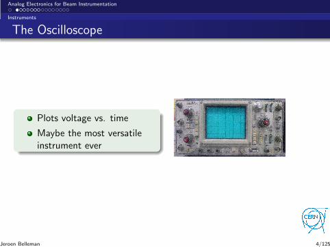
The Oscilloscope
Plots voltage vs. time
Maybe the most versatileinstrument ever
Jeroen Belleman 4/125
Analog Electronics for Beam Instrumentation
Instruments
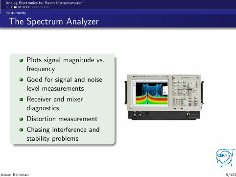
The Spectrum Analyzer
Plots signal magnitude vs.frequency
Good for signal and noiselevel measurements
Receiver and mixerdiagnostics,
Distortion measurement
Chasing interference andstability problems
Jeroen Belleman 5/125
Analog Electronics for Beam Instrumentation
Instruments
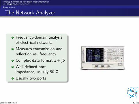
The Network Analyzer
Frequency-domain analysisof electrical networks
Measures transmission andreflection vs. frequency
Complex data format a+ jb
Well-defined portimpedance, usually 50 Ω
Usually two ports
Jeroen Belleman 6/125
Analog Electronics for Beam Instrumentation
Instruments
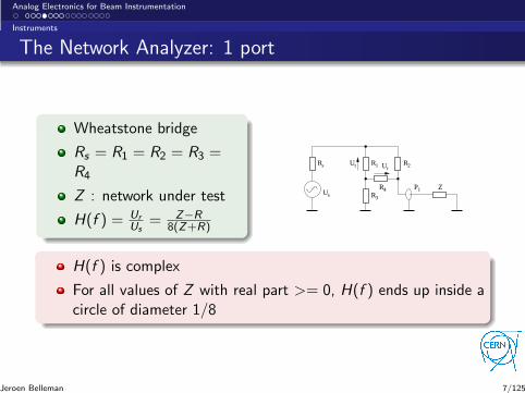
The Network Analyzer: 1 port
Wheatstone bridge
Rs = R1 = R2 = R3 =R4
Z : network under test
H(f ) = Ur
Us= Z−R
8(Z+R)
P1
Rs R1 R2
R3
R4
Ur
UsZ
Ut
H(f ) is complex
For all values of Z with real part >= 0, H(f ) ends up inside acircle of diameter 1/8
Jeroen Belleman 7/125
Analog Electronics for Beam Instrumentation
Instruments
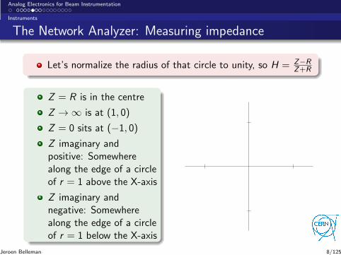
The Network Analyzer: Measuring impedance
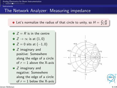
Let’s normalize the radius of that circle to unity, so H = Z−RZ+R
Z = R is in the centre
Z → ∞ is at (1, 0)
Z = 0 sits at (−1, 0)
Z imaginary andpositive: Somewherealong the edge of a circleof r = 1 above the X-axis
Z imaginary andnegative: Somewherealong the edge of a circleof r = 1 below the X-axis
Jeroen Belleman 8/125
Analog Electronics for Beam Instrumentation
Instruments
The Network Analyzer: Measuring impedance
Let’s normalize the radius of that circle to unity, so H = Z−RZ+R
Z = R is in the centre
Z → ∞ is at (1, 0)
Z = 0 sits at (−1, 0)
Z imaginary andpositive: Somewherealong the edge of a circleof r = 1 above the X-axis
Z imaginary andnegative: Somewherealong the edge of a circleof r = 1 below the X-axis
+1j
−1j
+0.5j +2j
−2j
+5j
−5j
12
50.50.2
−0.5j
−0.2j
+0.2j
0
Jeroen Belleman 9/125
Analog Electronics for Beam Instrumentation
Instruments
The Network Analyzer: Measuring transmission
P2P1
Rs R1 R2
R3
R4
Ur
Us
Ut
Rl
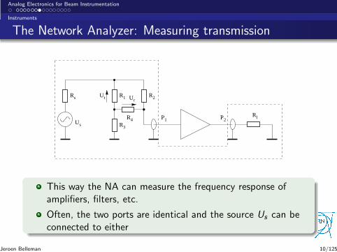
This way the NA can measure the frequency response ofamplifiers, filters, etc.
Often, the two ports are identical and the source Us can beconnected to either
Jeroen Belleman 10/125
Analog Electronics for Beam Instrumentation
Transmission Lines
Transmission Lines
Jeroen Belleman 11/125
Analog Electronics for Beam Instrumentation
Transmission Lines
Transmission lines
Confine EM fields between two conductors
Little radiation loss
Protected from interference
Propagation velocity set by material choice
Wave impedance set by geometry
Jeroen Belleman 12/125
Analog Electronics for Beam Instrumentation
Transmission Lines
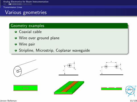
Various geometries
Geometry examples
Coaxial cable
Wire over ground plane
Wire pair
Stripline, Microstrip, Coplanar waveguide
b
a
dh h
D
d
Jeroen Belleman 13/125
Analog Electronics for Beam Instrumentation
Transmission Lines
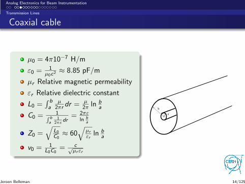
Coaxial cable
µ0 = 4π10−7 H/m
ε0 =1
µ0c2≈ 8.85 pF/m
µr Relative magnetic permeability
εr Relative dielectric constant
L0 =∫ b
aµ
2πr dr =µ
2π ln ba
C0 =1∫ b
a1
2πεdr
= 2πεln b
a
Z0 =√
L0C0
≈ 60√
µr
εrln b
a
v0 =1
L0C0= c√
µrεr
b
a
Jeroen Belleman 14/125
Analog Electronics for Beam Instrumentation
Transmission Lines
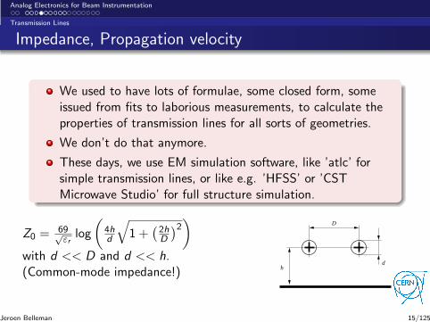
Impedance, Propagation velocity
We used to have lots of formulae, some closed form, someissued from fits to laborious measurements, to calculate theproperties of transmission lines for all sorts of geometries.
We don’t do that anymore.
These days, we use EM simulation software, like ’atlc’ forsimple transmission lines, or like e.g. ’HFSS’ or ’CSTMicrowave Studio’ for full structure simulation.
Z0 =69√εrlog
(
4hd
√
1 +(
2hD
)2)
with d << D and d << h.(Common-mode impedance!) h
D
d
Jeroen Belleman 15/125
Analog Electronics for Beam Instrumentation
Transmission Lines
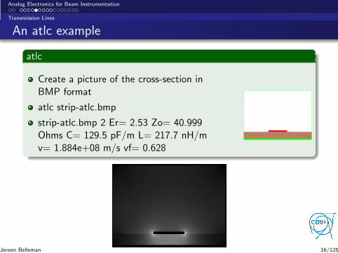
An atlc example
atlc
Create a picture of the cross-section inBMP format
atlc strip-atlc.bmp
strip-atlc.bmp 2 Er= 2.53 Zo= 40.999Ohms C= 129.5 pF/m L= 217.7 nH/mv= 1.884e+08 m/s vf= 0.628
Jeroen Belleman 16/125
Analog Electronics for Beam Instrumentation
Transmission Lines
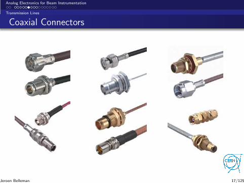
Coaxial Connectors
Jeroen Belleman 17/125
Analog Electronics for Beam Instrumentation
Transmission Lines
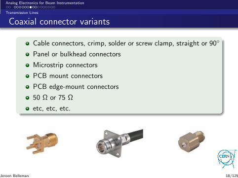
Coaxial connector variants
Cable connectors, crimp, solder or screw clamp, straight or 90
Panel or bulkhead connectors
Microstrip connectors
PCB mount connectors
PCB edge-mount connectors
50 Ω or 75 Ω
etc, etc, etc.
Jeroen Belleman 18/125
Analog Electronics for Beam Instrumentation
Transmission Lines
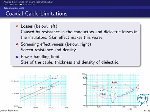
Coaxial Cable Limitations
Losses (below, left)Caused by resistance in the conductors and dielectric losses inthe insulators. Skin effect makes this worse.
Screening effectiveness (below, right)Screen resistance and density.
Power handling limitsSize of the cable, thickness and density of dielectric.
1 dB/100m
10 dB/100m
100 dB/100m
10MHz 100MHz 1GHz 10GHz
UT141
K01252D
RG142
RG225
Hz
Ω/µ
100u
1m
10m
100m
10k 100k 1M 10M 100M
RG58
CK50
CKB50 UT141
RG214
Jeroen Belleman 19/125
Analog Electronics for Beam Instrumentation
Transmission Lines
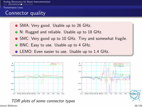
Connector quality
SMA: Very good. Usable up to 26 GHz.
N: Rugged and reliable. Usable up to 18 GHz.
SMC: Very good up to 10 GHz. Tiny and somewhat fragile.
BNC: Easy to use. Usable up to 4 GHz.
LEMO: Even easier to use. Usable up to 1.4 GHz.
ρ
−0.04
−0.02
0
0.02
0.04
0.0 s 200.0ps 400.0ps 600.0ps 800.0ps 1.0ns 1.2ns 1.4ns 1.6ns 1.8ns 2.0ns
’SMAterm.’’H+S−Nterm.’
ρ
−0.04
−0.02
0
0.02
0.04
0.0 s 200.0ps 400.0ps 600.0ps 800.0ps 1.0ns 1.2ns 1.4ns 1.6ns 1.8ns 2.0ns
’Radiall−SMCterm.’’Radiall−BNCterm.’’H+S−LEMOterm.’
TDR plots of some connector typesJeroen Belleman 20/125
Analog Electronics for Beam Instrumentation
Time Domain Reflectometry
Time Domain Reflectometry
Jeroen Belleman 21/125
Analog Electronics for Beam Instrumentation
Time Domain Reflectometry
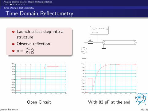
Time Domain Reflectometry
Launch a fast step into astructure
Observe reflection
ρ = R−Z0R+Z0
50
−300m
−250m
−200m
−150m
−100m
−50m
0
50m
100m
150m
200m
250m
0 2n 4n 6n 8n 10n 12n 14n 16n 18n 20n
Open Circuit
−30m
−25m
−20m
−15m
−10m
−5m
0
5m
10m
15m
0 5n 10n 15n 20n 25n 30n 35n 40n 45n 50n
With 82 pF at the end
Jeroen Belleman 22/125
Analog Electronics for Beam Instrumentation
Time Domain Reflectometry
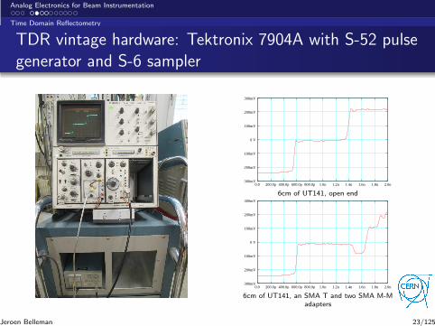
TDR vintage hardware: Tektronix 7904A with S-52 pulsegenerator and S-6 sampler
−300mV
−200mV
−100mV
0 V
100mV
200mV
300mV
0.0 200.0p 400.0p 600.0p 800.0p 1.0n 1.2n 1.4n 1.6n 1.8n 2.0n
6cm of UT141, open end
−300mV
−200mV
−100mV
0 V
100mV
200mV
300mV
0.0 200.0p 400.0p 600.0p 800.0p 1.0n 1.2n 1.4n 1.6n 1.8n 2.0n
6cm of UT141, an SMA T and two SMA M-Madapters
Jeroen Belleman 23/125
Analog Electronics for Beam Instrumentation
Time Domain Reflectometry
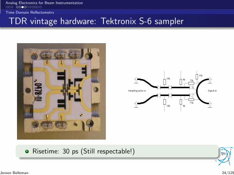
TDR vintage hardware: Tektronix S-6 sampler
16k
10k
75k
75k
4k16k
4k
Sampling pulse in Signal in
Risetime: 30 ps (Still respectable!)
Jeroen Belleman 24/125
Analog Electronics for Beam Instrumentation
Time Domain Reflectometry
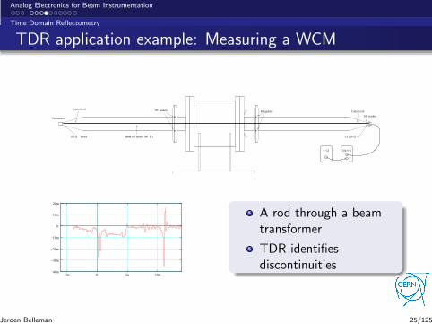
TDR application example: Measuring a WCM
T
Tek S−6S−52
Ω3 x 220 //Ω110 series
Terminator
6mm rod (about 160 )Ω
Conical rodConical rod
M3 washer
RF gasketsRF gaskets
−40m
−30m
−20m
−10m
0
10m
20m
−5n 0 5n 10n
A rod through a beamtransformer
TDR identifiesdiscontinuities
Jeroen Belleman 25/125
Analog Electronics for Beam Instrumentation
Transmission Line Transformers
Transmission line transformers
Jeroen Belleman 26/125
Analog Electronics for Beam Instrumentation
Transmission Line Transformers
Transmission line transformers
It’s possible to make very good transformers by exploitingtransmission line effects
Possible uses:
Scaling voltage, current and impedance
Impedance matching
Noise matching
Combiners and splitters
Single-ended ⇔ differential conversion
Feedback elements in low-noise amplifiers
Hybrids and directional couplers
...
Jeroen Belleman 27/125
Analog Electronics for Beam Instrumentation
Transmission Line Transformers
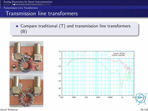
Transmission line transformers
Compare traditional (T) and transmission line transformers(B)
−50
−40
−30
−20
−10
0
10
10k 100k 1M 10M 100M 1G 10G
’xform−tlt.dat.’’xform−trad.dat.’
Jeroen Belleman 28/125
Analog Electronics for Beam Instrumentation
Transmission Line Transformers
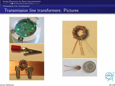
Transmission line transformers: Pictures
Jeroen Belleman 29/125
Analog Electronics for Beam Instrumentation
Transmission Line Transformers
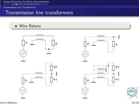
Transmission line transformers
Wire Baluns
R R
R R/2
R/2
R R
R R/2
R/2
Jeroen Belleman 30/125
Analog Electronics for Beam Instrumentation
Transmission Line Transformers
Transmission line transformers
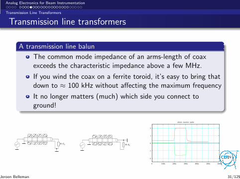
A transmission line balun
The common mode impedance of an arms-length of coaxexceeds the characteristic impedance above a few MHz.
If you wind the coax on a ferrite toroid, it’s easy to bring thatdown to ≈ 100 kHz without affecting the maximum frequency
It no longer matters (much) which side you connect toground!
R=Z0
R=Z0
−2
−1
0
1
2
0 100n 200n 300n 400n 500n 600n
xform−inverter−pulse
Jeroen Belleman 31/125
Analog Electronics for Beam Instrumentation
Transmission Line Transformers
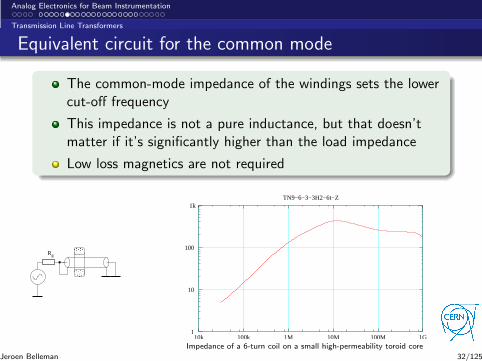
Equivalent circuit for the common mode
The common-mode impedance of the windings sets the lowercut-off frequency
This impedance is not a pure inductance, but that doesn’tmatter if it’s significantly higher than the load impedance
Low loss magnetics are not required
Rg
1
10
100
1k
10k 100k 1M 10M 100M 1G
TN9−6−3−3H2−6t−Z
Impedance of a 6-turn coil on a small high-permeability toroid core
Jeroen Belleman 32/125
Analog Electronics for Beam Instrumentation
Transmission Line Transformers
Transmission line transformers
It’s customary to specify the impedance ratio
... which is the square of the voltage ratio
The transmission line doesn’t have to be coax
Twisted pairsParallel wires
The lines may be wound as several turns on a single core
... or a single pass through several cores
... or some combination
Windings with the same common-mode voltage may sharecores
High µr cores extend LF cut-off frequency downward
Jeroen Belleman 33/125
Analog Electronics for Beam Instrumentation
Transmission Line Transformers
Transmission line transformers
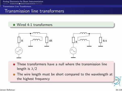
Wired 4-1 transformers
R 4R R R/4
These transformers have a null where the transmission linelength is λ/2
The wire length must be short compared to the wavelength atthe highest frequency
Jeroen Belleman 34/125
Analog Electronics for Beam Instrumentation
Transmission Line Transformers
Transmission line transformers
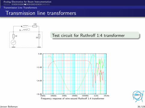
5050
150
Test circuit for Ruthroff 1:4 transformer
−36 dB
−24 dB
−12 dB
0 dB
10kHz 100kHz 1MHz 10MHz 100MHz 1GHz 10GHz
Frequency response of wire-wound Ruthroff 1-4 transformer
Jeroen Belleman 35/125
Analog Electronics for Beam Instrumentation
Transmission Line Transformers
Transmission line transformers
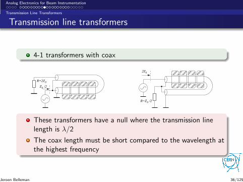
4-1 transformers with coax
R=2Z0
Z /20
R=Z /20
2Z0
These transformers have a null where the transmission linelength is λ/2
The coax length must be short compared to the wavelength atthe highest frequency
Jeroen Belleman 36/125
Analog Electronics for Beam Instrumentation
Transmission Line Transformers
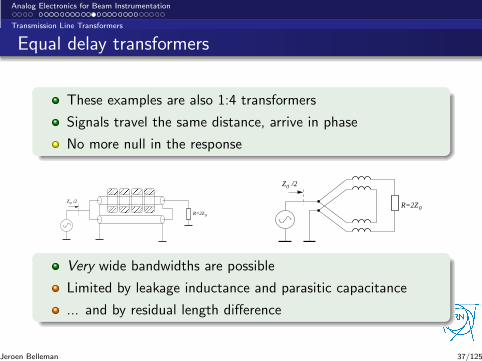
Equal delay transformers
These examples are also 1:4 transformers
Signals travel the same distance, arrive in phase
No more null in the response
Z /20
R=2Z0
R=2Z0
Z /20
Very wide bandwidths are possible
Limited by leakage inductance and parasitic capacitance
... and by residual length difference
Jeroen Belleman 37/125
Analog Electronics for Beam Instrumentation
Transmission Line Transformers
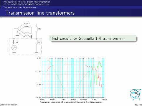
Transmission line transformers
50 50
150
Test circuit for Guanella 1-4 transformer
−36 dB
−24 dB
−12 dB
0 dB
10kHz 100kHz 1MHz 10MHz 100MHz 1GHz 10GHz
Frequency response of wire-wound Guanella 1-4 transformerJeroen Belleman 38/125
Analog Electronics for Beam Instrumentation
Transmission Line Transformers
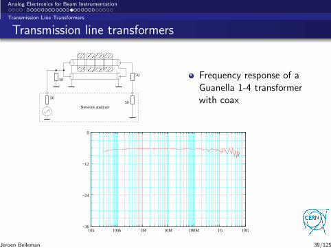
Transmission line transformers
5050
5050
Network analyzer
Frequency response of aGuanella 1-4 transformerwith coax
−36
−24
−12
0
10k 100k 1M 10M 100M 1G 10G
Jeroen Belleman 39/125
Analog Electronics for Beam Instrumentation
Transmission Line Transformers
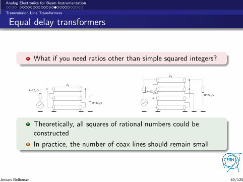
Equal delay transformers
What if you need ratios other than simple squared integers?
Z0
0R=2Z /3
R=3Z /20
Z0
0R=5Z /2R=2Z /50
Theoretically, all squares of rational numbers could beconstructed
In practice, the number of coax lines should remain small
Jeroen Belleman 40/125
Analog Electronics for Beam Instrumentation
Transmission Line Transformers
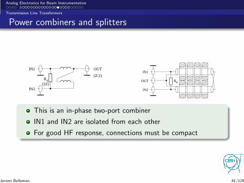
Power combiners and splitters
Rd
IN1
IN2
OUT
(Z/2)
(2Z)
Rd
IN1
OUT
IN2
This is an in-phase two-port combiner
IN1 and IN2 are isolated from each other
For good HF response, connections must be compact
Jeroen Belleman 41/125

Analog Electronics for Beam Instrumentation
Transmission Line Transformers
Power combiners and splitters
Rs
IN1 (Z)
IN2 (Z)
(Z/2)OUT (2Z)
IN1
IN2
Σ
∆ (Z/2)
(Z/2)
A 180 two-port combiner (left) and a hybrid (right)
IN1 and IN2 are isolated from each other
For good HF response, connections must be compact
Jeroen Belleman 42/125
Analog Electronics for Beam Instrumentation
Transmission Line Transformers
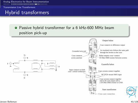
Hybrid transformers
Passive hybrid transformer for a 6 kHz-600 MHz beamposition pick-up
X+
X−
Σ
∆
Balun outputs cross−connect50 Ohm SMD resistor between screens
Grounded wire end
Coax connects
through the ferrites as the coaxAn insulated wire follows the same path
Coax connects to difference output
90° PCB−mount SMA input
Coax screens connect together
Coax screens connect together
coax’ central conductors
Cross−over connection
Guanella balun
Output balun
Sum transformer
and to the sum output and toa 50 Ohm SMD resistor to GND
Input connects to both
across junction
Jeroen Belleman 43/125
Analog Electronics for Beam Instrumentation
Transmission Line Transformers
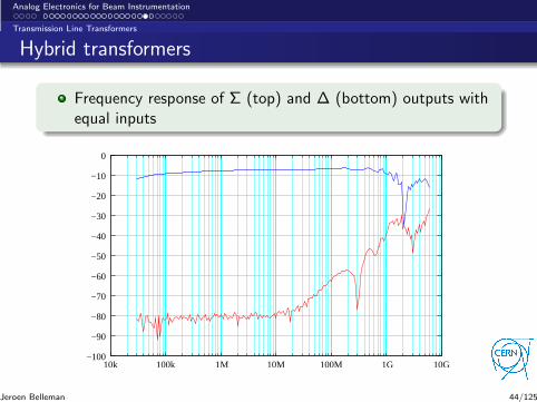
Hybrid transformers
Frequency response of Σ (top) and ∆ (bottom) outputs withequal inputs
−100
−90
−80
−70
−60
−50
−40
−30
−20
−10
0
10k 100k 1M 10M 100M 1G 10G
Jeroen Belleman 44/125
Analog Electronics for Beam Instrumentation
Transmission Line Transformers
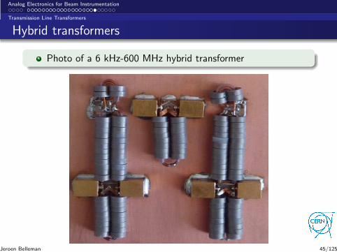
Hybrid transformers
Photo of a 6 kHz-600 MHz hybrid transformer
Jeroen Belleman 45/125
Analog Electronics for Beam Instrumentation
Passive LC Filters
Passive LC filters
Jeroen Belleman 46/125
Analog Electronics for Beam Instrumentation
Passive LC Filters
Passive LC filters
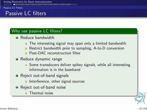
Why use passive LC filters?
Reduce bandwidth
The interesting signal may span only a limited bandwidthRestrict bandwidth prior to sampling, A-to-D conversionPost-DAC reconstruction filter
Reduce dynamic range
Some transducers deliver spikey signals, while all interestinginformation is in the baseband
Reject out-of-band signals
Interference, other signal sources
Reject out-of-band noise
Thermal noise
Jeroen Belleman 47/125
Analog Electronics for Beam Instrumentation
Passive LC Filters
LC low-pass prototypes
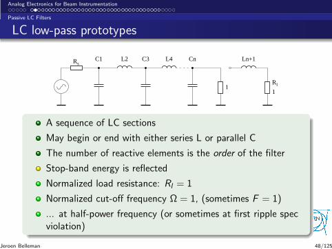
Rl
Rs
1
C1 L2 C3 L4 Cn Ln+1
1
A sequence of LC sections
May begin or end with either series L or parallel C
The number of reactive elements is the order of the filter
Stop-band energy is reflected
Normalized load resistance: Rl = 1
Normalized cut-off frequency Ω = 1, (sometimes F = 1)
... at half-power frequency (or sometimes at first ripple specviolation)
Jeroen Belleman 48/125
Analog Electronics for Beam Instrumentation
Passive LC Filters
Filter families
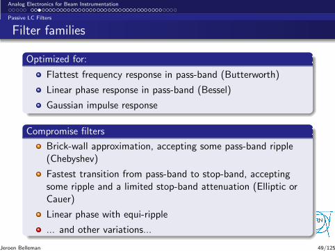
Optimized for:
Flattest frequency response in pass-band (Butterworth)
Linear phase response in pass-band (Bessel)
Gaussian impulse response
Compromise filters
Brick-wall approximation, accepting some pass-band ripple(Chebyshev)
Fastest transition from pass-band to stop-band, acceptingsome ripple and a limited stop-band attenuation (Elliptic orCauer)
Linear phase with equi-ripple
... and other variations...
Jeroen Belleman 49/125
Analog Electronics for Beam Instrumentation
Passive LC Filters
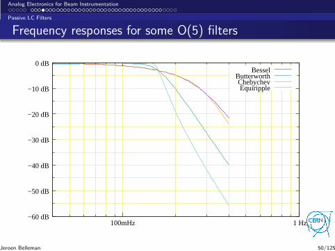
Frequency responses for some O(5) filters
BesselButterworthChebychevEquiripple
−60 dB
−50 dB
−40 dB
−30 dB
−20 dB
−10 dB
0 dB
100mHz 1 Hz
Jeroen Belleman 50/125
Analog Electronics for Beam Instrumentation
Passive LC Filters
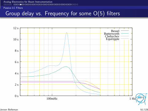
Group delay vs. Frequency for some O(5) filters
BesselButterworthChebychevEquiripple
0 s
2 s
4 s
6 s
8 s
10 s
12 s
100mHz 1 Hz
Jeroen Belleman 51/125
Analog Electronics for Beam Instrumentation
Passive LC Filters
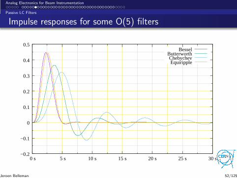
Impulse responses for some O(5) filters
BesselButterworthChebychevEquiripple
−0.2
−0.1
0
0.1
0.2
0.3
0.4
0.5
0 s 5 s 10 s 15 s 20 s 25 s 30 s
Jeroen Belleman 52/125
Analog Electronics for Beam Instrumentation
Passive LC Filters
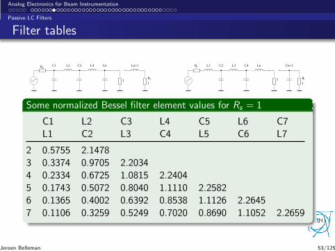
Filter tables
Rl
Rs
1
C1 L2 C3 L4 Cn Ln+1
1
Rs
1
Cn+1L1 C2 L3 C4 Ln
1
Rl
Some normalized Bessel filter element values for Rs = 1
C1 L2 C3 L4 C5 L6 C7L1 C2 L3 C4 L5 C6 L7
2 0.5755 2.14783 0.3374 0.9705 2.20344 0.2334 0.6725 1.0815 2.24045 0.1743 0.5072 0.8040 1.1110 2.25826 0.1365 0.4002 0.6392 0.8538 1.1126 2.26457 0.1106 0.3259 0.5249 0.7020 0.8690 1.1052 2.2659
Jeroen Belleman 53/125
Analog Electronics for Beam Instrumentation
Passive LC Filters
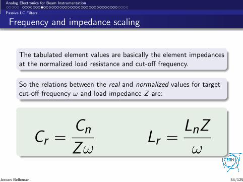
Frequency and impedance scaling
The tabulated element values are basically the element impedancesat the normalized load resistance and cut-off frequency.
So the relations between the real and normalized values for targetcut-off frequency ω and load impedance Z are:
Cr =Cn
ZωLr =
LnZ
ω
Jeroen Belleman 54/125
Analog Electronics for Beam Instrumentation
Passive LC Filters
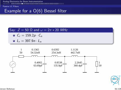
Example for a O(6) Bessel filter
Say: Z = 50 Ω and ω = 2π ∗ 20 MHz
Cr = 159.2p · Cn
Lr = 397.9n · Ln
50
54.32nH 254.3nH 442.7nH
0.400263.69pF
0.8538135.9pF
2.2645360.4pF
501 0.1365 0.6392 1.1126
1
Jeroen Belleman 55/125
Analog Electronics for Beam Instrumentation
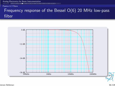
Passive LC Filters
Frequency response of the Bessel O(6) 20 MHz low-passfilter
−36 dB
−24 dB
−12 dB
0 dB
100kHz 1MHz 10MHz 100MHz
Jeroen Belleman 56/125
Analog Electronics for Beam Instrumentation
Passive LC Filters
Finishing up the filter design
You can’t have 4-digit accurate inductors and capacitors.
Common L’s and C’s have values in the E12 series (≈ 20 %steps from one value to the next) and 5 % tolerances.
You have to select from standard values.
You may obtain a slightly better approximation by series orparallel combinations of two components but you’ll still belimited by the basic component tolerances
Depending on frequency and impedance choices, elementvalues may end up impractically large or small
Jeroen Belleman 57/125
Analog Electronics for Beam Instrumentation
Passive LC Filters
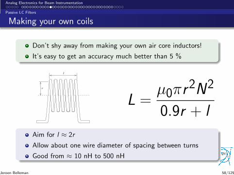
Making your own coils
Don’t shy away from making your own air core inductors!
It’s easy to get an accuracy much better than 5 %
l
r
L =µ0πr
2N2
0.9r + l
Aim for l ≈ 2r
Allow about one wire diameter of spacing between turns
Good from ≈ 10 nH to 500 nH
Jeroen Belleman 58/125
Analog Electronics for Beam Instrumentation
Passive LC Filters
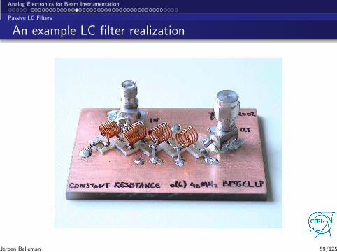
An example LC filter realization
Jeroen Belleman 59/125
Analog Electronics for Beam Instrumentation
Passive LC Filters
Bandpass filters
The same filter element tables can be used to design bandpassfilters
You start off by designing a low-pass filter with a cut-offfrequency at the target bandwidth.
Then you replace each series component with a series L-Ccombination and each parallel component with a parallel L-C,both tuned to the desired centre frequency.
Jeroen Belleman 60/125
Analog Electronics for Beam Instrumentation
Passive LC Filters
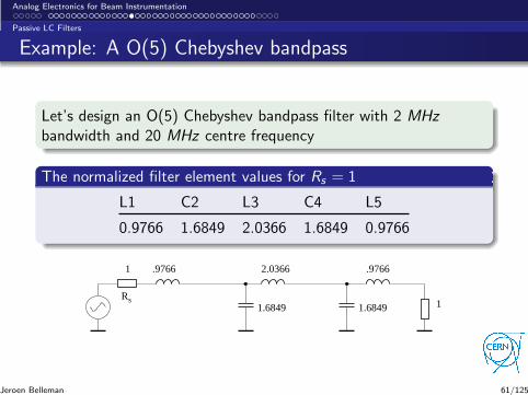
Example: A O(5) Chebyshev bandpass
Let’s design an O(5) Chebyshev bandpass filter with 2 MHz
bandwidth and 20 MHz centre frequency
The normalized filter element values for Rs = 1
L1 C2 L3 C4 L5
0.9766 1.6849 2.0366 1.6849 0.9766
.9766 2.0366 .9766
1.6849
1
11.6849Rs
Jeroen Belleman 61/125
Analog Electronics for Beam Instrumentation
Passive LC Filters
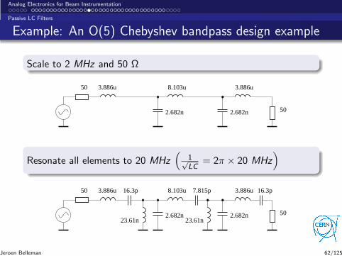
Example: An O(5) Chebyshev bandpass design example
Scale to 2 MHz and 50 Ω
50
2.682n
3.886u 8.103u
50
3.886u
2.682n
Resonate all elements to 20 MHz(
1√LC
= 2π × 20 MHz)
50
2.682n
3.886u 8.103u
50
3.886u
2.682n
16.3p 16.3p
23.61n23.61n
7.815p
Jeroen Belleman 62/125
Analog Electronics for Beam Instrumentation
Passive LC Filters
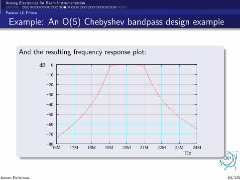
Example: An O(5) Chebyshev bandpass design example
And the resulting frequency response plot:
dB
Hz
−80
−70
−60
−50
−40
−30
−20
−10
0
16M 17M 18M 19M 20M 21M 22M 23M 24M
Jeroen Belleman 63/125
Analog Electronics for Beam Instrumentation
Passive LC Filters
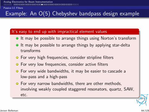
Example: An O(5) Chebyshev bandpass design example
It’s easy to end up with impractical element values
It may be possible to arrange things using Norton’s transform
It may be possible to arrange things by applying star-deltatransforms
For very high frequencies, consider stripline filters
For very low frequencies, consider active filters
For very wide bandwidths, it may be easier to cascade alow-pass and a high-pass
For very narrow bandwidths, there are other methods,involving weakly coupled staggered resonators, quartz, SAW,etc.
Jeroen Belleman 64/125
Analog Electronics for Beam Instrumentation
Passive LC Filters
Intermezzo: Parasitics
Capacitance to floating nodes
Capacitance and inductance of resistors
Parasitic inductance and resistance of capacitors
Self-capacitance and resistance in inductances
Undesired inductive coupling
Jeroen Belleman 65/125
Analog Electronics for Beam Instrumentation
Passive LC Filters
Resistors
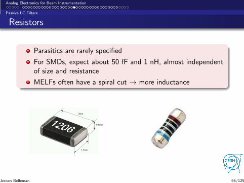
Parasitics are rarely specified
For SMDs, expect about 50 fF and 1 nH, almost independentof size and resistance
MELFs often have a spiral cut → more inductance
3mm
1.5mm
0.6mm
Jeroen Belleman 66/125
Analog Electronics for Beam Instrumentation
Passive LC Filters
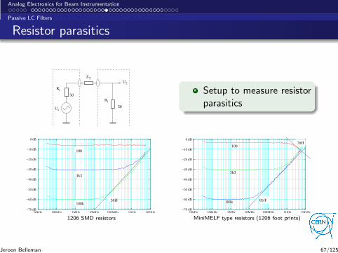
Resistor parasitics
50
50
Rs
Rl
ZT
Us
U2
Setup to measure resistorparasitics
100
3k3
100k50fF
−70 dB
−60 dB
−50 dB
−40 dB
−30 dB
−20 dB
−10 dB
0 dB
10kHz 100kHz 1MHz 10MHz 100MHz 1GHz 10GHz
1206 SMD resistors
85fF
100
100k
3k3
7nH
−70 dB
−60 dB
−50 dB
−40 dB
−30 dB
−20 dB
−10 dB
0 dB
10kHz 100kHz 1MHz 10MHz 100MHz 1GHz 10GHz
MiniMELF type resistors (1206 foot prints)
Jeroen Belleman 67/125
Analog Electronics for Beam Instrumentation
Passive LC Filters
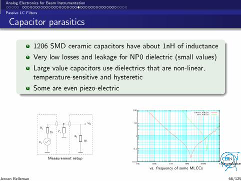
Capacitor parasitics
1206 SMD ceramic capacitors have about 1nH of inductance
Very low losses and leakage for NP0 dielectric (small values)
Large value capacitors use dielectrics that are non-linear,temperature-sensitive and hysteretic
Some are even piezo-electric
Zt50
50
Rs
Rl
Us
U2
Measurement setup 0.01
0.1
1
10
100
10k 100k 1M 10M 100M 1G
’100n−1206.dat.’’1n−1206.dat.’
Impedancevs. frequency of some MLCCs
Jeroen Belleman 68/125
Analog Electronics for Beam Instrumentation
Passive LC Filters
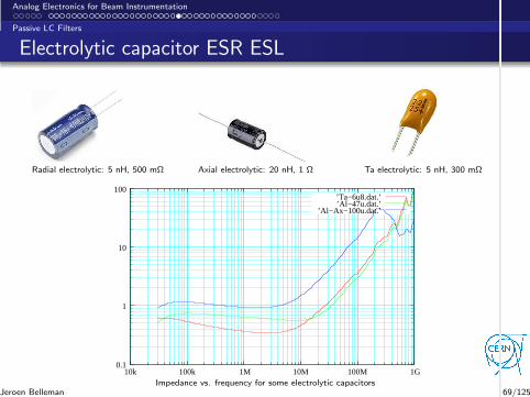
Electrolytic capacitor ESR ESL
Radial electrolytic: 5 nH, 500 mΩ Axial electrolytic: 20 nH, 1 Ω Ta electrolytic: 5 nH, 300 mΩ
0.1
1
10
100
10k 100k 1M 10M 100M 1G
’Ta−6u8.dat.’’Al−47u.dat.’
’Al−Ax−100u.dat.’
Impedance vs. frequency for some electrolytic capacitorsJeroen Belleman 69/125
Analog Electronics for Beam Instrumentation
Passive LC Filters
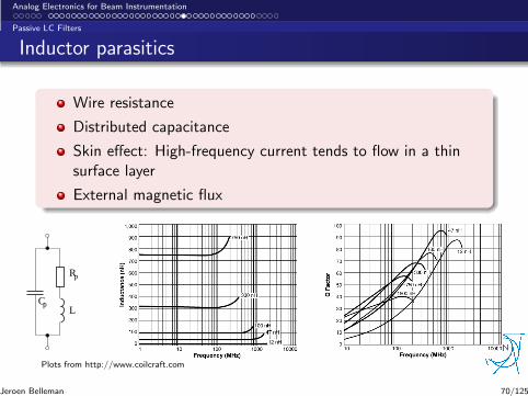
Inductor parasitics
Wire resistance
Distributed capacitance
Skin effect: High-frequency current tends to flow in a thinsurface layer
External magnetic flux
Cp
Rp
L
Plots from http://www.coilcraft.com
Jeroen Belleman 70/125
Analog Electronics for Beam Instrumentation
Passive LC Filters
Back to passive Filters
Jeroen Belleman 71/125
Analog Electronics for Beam Instrumentation
Passive LC Filters
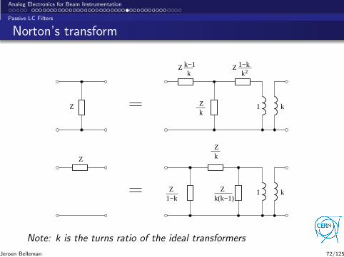
Norton’s transform
k−1Zk k2
Z 1−k
Z Z 1 kk
1 k
Z
Zk
Z1−k k(k−1)
Z
Note: k is the turns ratio of the ideal transformers
Jeroen Belleman 72/125
Analog Electronics for Beam Instrumentation
Passive LC Filters
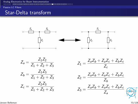
Star-Delta transform
Za Zb
Zc
Z1
Z2 Z3
Za =Z1Z2
Z1 + Z2 + Z3
Zb =Z1Z3
Z1 + Z2 + Z3
Zc =Z2Z3
Z1 + Z2 + Z3
Z1 =ZaZb + ZaZc + ZbZc
Zc
Z2 =ZaZb + ZaZc + ZbZc
Zb
Z3 =ZaZb + ZaZc + ZbZc
Za
Jeroen Belleman 73/125
Analog Electronics for Beam Instrumentation
Passive LC Filters
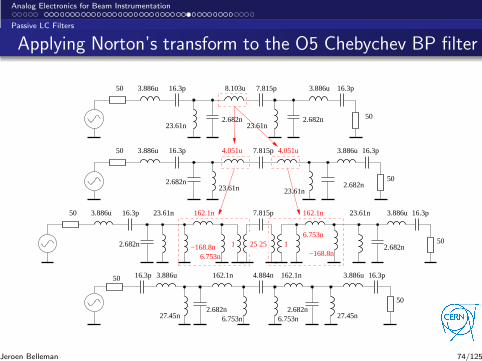
Applying Norton’s transform to the O5 Chebychev BP filter
1 25
162.1n
2.682n
50 3.886u 16.3p
125
7.815p
50
16.3p3.886u
2.682n
50 3.886u 16.3p
502.682n23.61n 2.682n
23.61n
16.3p3.886u4.051u7.815p
50
2.682n
3.886u 8.103u
50
3.886u
2.682n
16.3p 16.3p
23.61n23.61n
7.815p
4.051u
162.1n23.61n 23.61n
50
50
16.3p4.884n
27.45n 27.45n2.682n2.682n
16.3p 3.886u 162.1n 162.1n 3.886u
6.753n 6.753n
−168.8n6.753n −168.8n
6.753n
Jeroen Belleman 74/125
Analog Electronics for Beam Instrumentation
Passive LC Filters
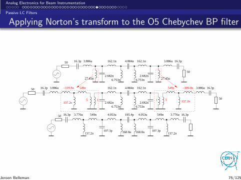
Applying Norton’s transform to the O5 Chebychev BP filter
4.884n
2.682n2.682n
162.1n 162.1n
6.753n 6.753n
15
50 16.3p 3.886u
137.2n
549n−109.8n
1 5 137.2n
549n −109.8n
50
16.3p3.886u
4.053u
168.8n
195.4p 4.053u
107.3p 168.8n 107.3p
50
50
16.3p4.884n
27.45n 27.45n2.682n2.682n
16.3p 3.886u 162.1n 162.1n 3.886u
6.753n 6.753n
16.3p50 16.3p 549n3.776u 3.776u549n
137.2n 137.2n
Jeroen Belleman 75/125
Analog Electronics for Beam Instrumentation
Passive LC Filters
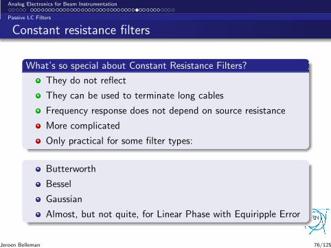
Constant resistance filters
What’s so special about Constant Resistance Filters?
They do not reflect
They can be used to terminate long cables
Frequency response does not depend on source resistance
More complicated
Only practical for some filter types:
Butterworth
Bessel
Gaussian
Almost, but not quite, for Linear Phase with Equiripple Error
Jeroen Belleman 76/125
Analog Electronics for Beam Instrumentation
Passive LC Filters
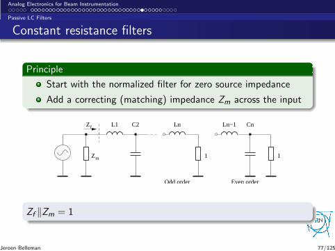
Constant resistance filters
Principle
Start with the normalized filter for zero source impedance
Add a correcting (matching) impedance Zm across the input
Zf
Zm
LnC2L1 Ln−1 Cn
1 1
Odd order Even order
Zf ‖Zm = 1
Jeroen Belleman 77/125
Analog Electronics for Beam Instrumentation
Passive LC Filters
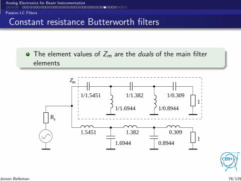
Constant resistance Butterworth filters
The element values of Zm are the duals of the main filterelements
Zm
1
1
1.6944
1/1.5451 1/1.382 1/0.309
1/0.89441/1.6944
1.5451 1.382 0.309
0.8944
Rs
Jeroen Belleman 78/125
Analog Electronics for Beam Instrumentation
Passive LC Filters
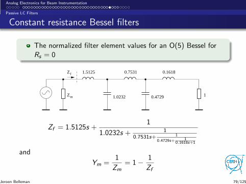
Constant resistance Bessel filters
The normalized filter element values for an O(5) Bessel forRs = 0
Zf
1
1.5125 0.7531 0.1618
0.47291.0232Zm
Zf = 1.5125s +1
1.0232s + 10.7531s+ 1
0.4729s+ 10.1618s+1
and
Ym =1
Zm
= 1− 1
Zf
Jeroen Belleman 79/125
Analog Electronics for Beam Instrumentation
Passive LC Filters
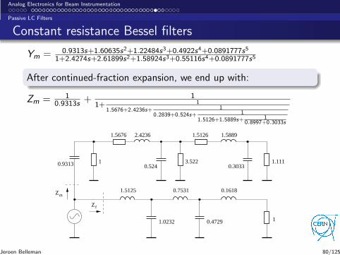
Constant resistance Bessel filters
Ym = 0.9313s+1.60635s2+1.22484s3+0.4922s4+0.0891777s5
1+2.4274s+2.61899s2+1.58924s3+0.55116s4+0.0891777s5
After continued-fraction expansion, we end up with:
Zm = 10.9313s +
11+ 1
1.5676+2.4236s+ 1
0.2839+0.524s+ 1
1.5126+1.5889s+ 10.8997+0.3033s
Zf
Zm
1
1.5125 0.7531 0.1618
0.47291.0232
0.9313 1
1.5676 2.4236
0.5243.522
1.5126 1.5889
0.30331.111
Jeroen Belleman 80/125
Analog Electronics for Beam Instrumentation
Passive LC Filters
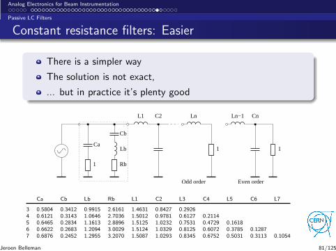
Constant resistance filters: Easier
There is a simpler way
The solution is not exact,
... but in practice it’s plenty good
Odd order Even order
LnC2L1 Ln−1 Cn
1
Cb
Lb
Rb
Ca1 1
Ca Cb Lb Rb L1 C2 L3 C4 L5 C6 L7
3 0.5804 0.3412 0.9915 2.6161 1.4631 0.8427 0.29264 0.6121 0.3143 1.0646 2.7036 1.5012 0.9781 0.6127 0.21145 0.6465 0.2834 1.1613 2.8896 1.5125 1.0232 0.7531 0.4729 0.16186 0.6622 0.2683 1.2094 3.0029 1.5124 1.0329 0.8125 0.6072 0.3785 0.12877 0.6876 0.2452 1.2955 3.2070 1.5087 1.0293 0.8345 0.6752 0.5031 0.3113 0.1054
Jeroen Belleman 81/125
Analog Electronics for Beam Instrumentation
Passive LC Filters
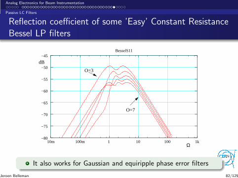
Reflection coefficient of some ’Easy’ Constant ResistanceBessel LP filters
Ω
dB
O=3
O=7
−80
−75
−70
−65
−60
−55
−50
−45
10m 100m 1 10 100 1k
BesselS11
It also works for Gaussian and equiripple phase error filters
Jeroen Belleman 82/125
Analog Electronics for Beam Instrumentation
Constant Resistance Networks
Constant Resistance Networks
Jeroen Belleman 83/125
Analog Electronics for Beam Instrumentation
Constant Resistance Networks
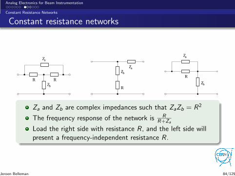
Constant resistance networks
aZ
R RZb
aZZb
R
aZ
bZ
R
Za and Zb are complex impedances such that ZaZb = R2
The frequency response of the network is RR+Za
Load the right side with resistance R , and the left side willpresent a frequency-independent resistance R .
Jeroen Belleman 84/125
Analog Electronics for Beam Instrumentation
Constant Resistance Networks
Constant resistance networks
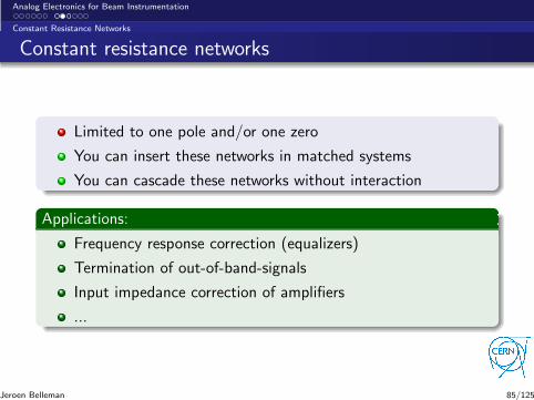
Limited to one pole and/or one zero
You can insert these networks in matched systems
You can cascade these networks without interaction
Applications:
Frequency response correction (equalizers)
Termination of out-of-band-signals
Input impedance correction of amplifiers
...
Jeroen Belleman 85/125
Analog Electronics for Beam Instrumentation
Constant Resistance Networks
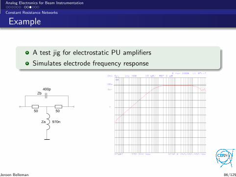
Example
A test jig for electrostatic PU amplifiers
Simulates electrode frequency response
50 50
400p
970n
Zb
Za
Jeroen Belleman 86/125
Analog Electronics for Beam Instrumentation
Noise in electronics
Noise in electronics
Jeroen Belleman 87/125
Analog Electronics for Beam Instrumentation
Noise in electronics
Noise
By noise I mean undesired fluctuations intrinsic in a device
Thermal noiseShot noise
Undesired fluctuations coming from outside are interference
Radio frequency interference (RFI)Power supply noise...
Jeroen Belleman 88/125
Analog Electronics for Beam Instrumentation
Noise in electronics
Thermal or Johnson noise
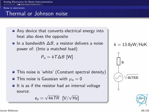
Any device that converts electrical energy intoheat also does the opposite
In a bandwidth ∆B , a resistor delivers a noisepower of: (Into a matched load)
Pn = kT∆B [W]
This noise is ’white’ (Constant spectral density)
This noise is Gaussian with µn = 0
It is as if the resistor had an internal voltagesource:
en =√4kTR [V/
√Hz]
k = 13.8yW/HzK
4kTRB
R
Jeroen Belleman 89/125
Analog Electronics for Beam Instrumentation
Noise in electronics
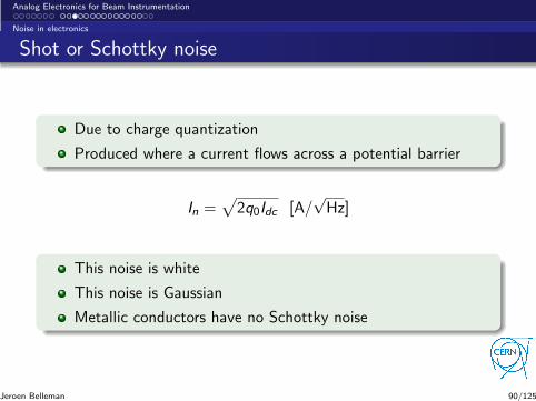
Shot or Schottky noise
Due to charge quantization
Produced where a current flows across a potential barrier
In =√
2q0Idc [A/√Hz]
This noise is white
This noise is Gaussian
Metallic conductors have no Schottky noise
Jeroen Belleman 90/125
Analog Electronics for Beam Instrumentation
Noise in electronics
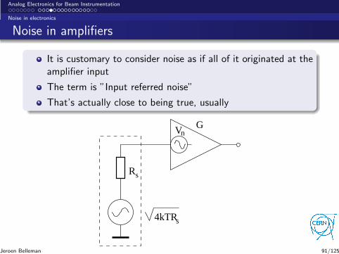
Noise in amplifiers
It is customary to consider noise as if all of it originated at theamplifier input
The term is ”Input referred noise”
That’s actually close to being true, usually
Rs
4kTRs
GVn
Jeroen Belleman 91/125
Analog Electronics for Beam Instrumentation
Noise in electronics
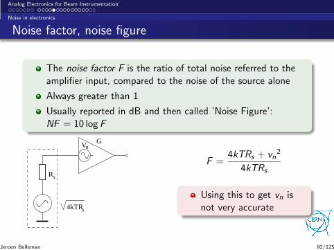
Noise factor, noise figure
The noise factor F is the ratio of total noise referred to theamplifier input, compared to the noise of the source alone
Always greater than 1
Usually reported in dB and then called ’Noise Figure’:NF = 10 log F
Rs
4kTRs
GVn
F =4kTRs + vn
2
4kTRs
Using this to get vn isnot very accurate
Jeroen Belleman 92/125
Analog Electronics for Beam Instrumentation
Noise in electronics
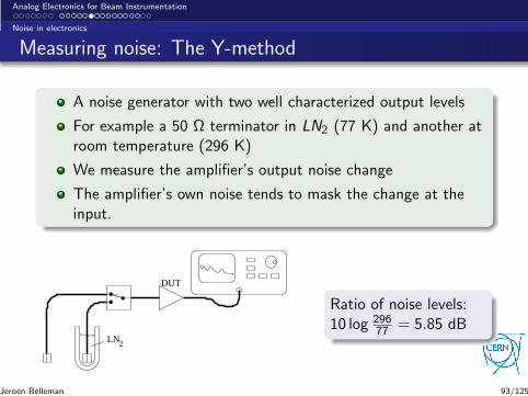
Measuring noise: The Y-method
A noise generator with two well characterized output levels
For example a 50 Ω terminator in LN2 (77 K) and another atroom temperature (296 K)
We measure the amplifier’s output noise change
The amplifier’s own noise tends to mask the change at theinput.
LN2
DUT
Ratio of noise levels:10 log 296
77 = 5.85 dB
Jeroen Belleman 93/125
Analog Electronics for Beam Instrumentation
Noise in electronics
Measuring noise: The Y-method
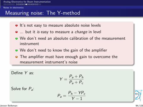
It’s not easy to measure absolute noise levels
... but it is easy to measure a change in level
We don’t need an absolute calibration of the measurementinstrument
We don’t need to know the gain of the amplifier
The amplifier must have enough gain to overcome themeasurement instrument’s noise
Define Y as:
Y =Pa + Ph
Pa + Pc
Solve for Pa:
Pa =Ph − YPc
Y − 1
Jeroen Belleman 94/125
Analog Electronics for Beam Instrumentation
Noise in electronics
Measuring noise: The Y-method
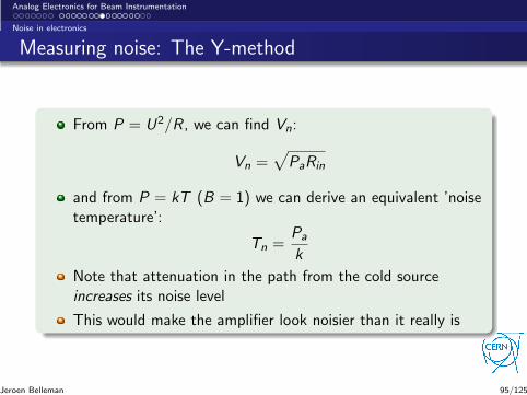
From P = U2/R , we can find Vn:
Vn =√
PaRin
and from P = kT (B = 1) we can derive an equivalent ’noisetemperature’:
Tn =Pa
k
Note that attenuation in the path from the cold sourceincreases its noise level
This would make the amplifier look noisier than it really is
Jeroen Belleman 95/125
Analog Electronics for Beam Instrumentation
Noise in electronics
Measuring noise: The Y-method
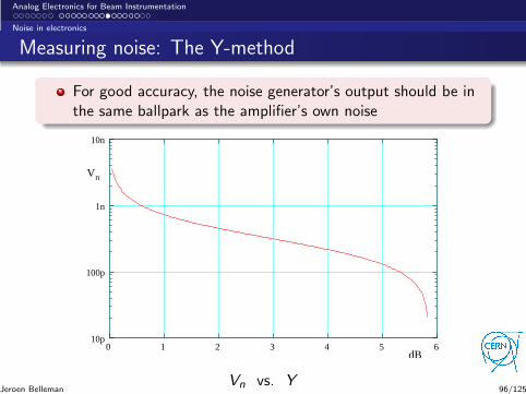
For good accuracy, the noise generator’s output should be inthe same ballpark as the amplifier’s own noise
dB
Vn
10p
100p
1n
10n
0 1 2 3 4 5 6
Vn vs. YJeroen Belleman 96/125
Analog Electronics for Beam Instrumentation
Noise in electronics
Noise in bipolar transistors
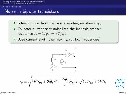
Johnson noise from the base spreading resistance rbb
Collector current shot noise into the intrinsic emitterresistance re = 1/gm = kT/qIc
Base current shot noise into rbb (at low frequencies)
en
in
Rs
Vs
en =
√
4kTrbb + 2qIc r2e +2qIcβ
r2bb ≈√
4kTrbb + 2kTre
Jeroen Belleman 97/125
Analog Electronics for Beam Instrumentation
Noise in electronics
Noise in FETs
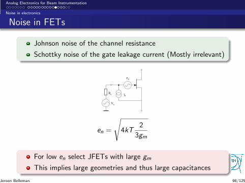
Johnson noise of the channel resistance
Schottky noise of the gate leakage current (Mostly irrelevant)
en
inRs
Vs
en =
√
4kT2
3gm
For low en select JFETs with large gm
This implies large geometries and thus large capacitances
Jeroen Belleman 98/125
Analog Electronics for Beam Instrumentation
Noise in electronics
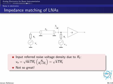
Impedance matching of LNAs
Z i
RtRs
Vs e n
Z0
−A
Input referred noise voltage density due to Rt :
vn =√4kTRt
(
Rs
Rs+Rt
)
=√kTRt
Not so great!
Jeroen Belleman 99/125
Analog Electronics for Beam Instrumentation
Noise in electronics
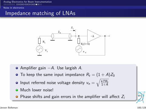
Impedance matching of LNAs
Z i
tR (1+A)Rs
Vs e n
Z0
−A
Amplifier gain −A. Use largish A.
To keep the same input impedance Rt = (1 + A)Z0
Input referred noise voltage density vn =√
kTRt
1+A
Much lower noise!
Phase shifts and gain errors in the amplifier will affect Zi
Jeroen Belleman 100/125
Analog Electronics for Beam Instrumentation
Noise in electronics
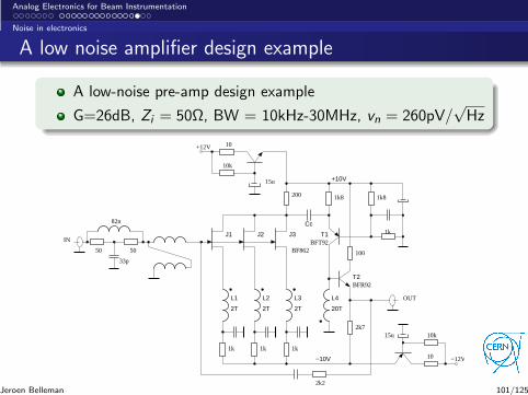
A low noise amplifier design example
A low-noise pre-amp design example
G=26dB, Zi = 50Ω, BW = 10kHz-30MHz, vn = 260pV/√Hz
T1
Cc
L4
20T2T
J1
L1
2T
J2
2T
L2 L3
J3
T2
+10V
−10V
1k
2k7
100
1k8200
1k 1k
2k2
1k8
1k
BF862
BFR92
BFT92
10k
15u
10+12V
−12V
10k
10
15u
50 50
82n
33p
IN
OUT
Jeroen Belleman 101/125
Analog Electronics for Beam Instrumentation
Electromagnetic Interference
Electromagnetic Interference
Jeroen Belleman 102/125
Analog Electronics for Beam Instrumentation
Electromagnetic Interference
Electromagnetic interference
Unwanted signals from outside leaking into your system
Often difficult to fix:
The source is unknownThe coupling path is unknownThe critical components do not appear in any schematicdiagram... and may not even be actual components
Jeroen Belleman 103/125
Analog Electronics for Beam Instrumentation
Electromagnetic Interference
Coupling mechanisms
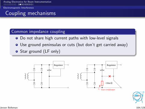
Common impedance coupling
Do not share high current paths with low-level signals
Use ground peninsulas or cuts (but don’t get carried away)
Star ground (LF only)
Regulator Regulator
~10mΩ
trace resistance
Jeroen Belleman 104/125
Analog Electronics for Beam Instrumentation
Electromagnetic Interference
Coupling mechanisms
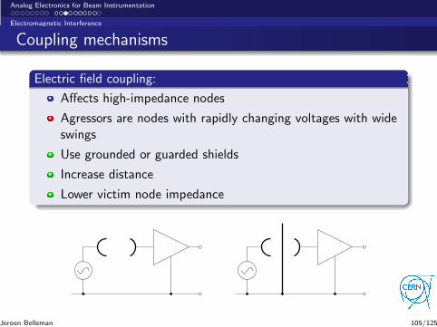
Electric field coupling:
Affects high-impedance nodes
Agressors are nodes with rapidly changing voltages with wideswings
Use grounded or guarded shields
Increase distance
Lower victim node impedance
Jeroen Belleman 105/125
Analog Electronics for Beam Instrumentation
Electromagnetic Interference
Magnetic coupling:
Affects loops
Keep loops with high currents small
Keep victim loops small
Put distance between them
Screening is difficult
Jeroen Belleman 106/125
Analog Electronics for Beam Instrumentation
Electromagnetic Interference
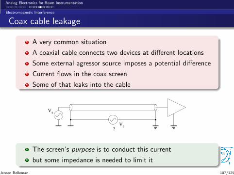
Coax cable leakage
A very common situation
A coaxial cable connects two devices at different locations
Some external agressor source imposes a potential difference
Current flows in the coax screen
Some of that leaks into the cable
Vs
Va?
The screen’s purpose is to conduct this current
but some impedance is needed to limit it
Jeroen Belleman 107/125
Analog Electronics for Beam Instrumentation
Electromagnetic Interference
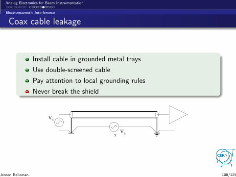
Coax cable leakage
Install cable in grounded metal trays
Use double-screened cable
Pay attention to local grounding rules
Never break the shield
Vs
Va?
Jeroen Belleman 108/125
Analog Electronics for Beam Instrumentation
Electromagnetic Interference
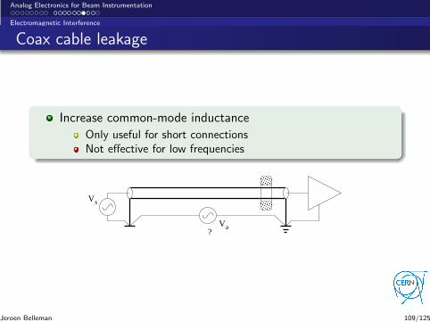
Coax cable leakage
Increase common-mode inductance
Only useful for short connectionsNot effective for low frequencies
Vs
Va
?
Jeroen Belleman 109/125
Analog Electronics for Beam Instrumentation
Electromagnetic Interference
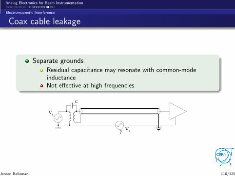
Coax cable leakage
Separate grounds
Residual capacitance may resonate with common-modeinductanceNot effective at high frequencies
Vs
Va?
C
Jeroen Belleman 110/125
Analog Electronics for Beam Instrumentation
Electromagnetic Interference
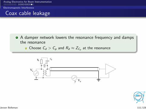
Coax cable leakage
A damper network lowers the resonance frequency and dampsthe resonance
Choose Cd > Cp and Rd ≈ ZCpat the resonance
Vs
Va
RdCd
?
C
Jeroen Belleman 111/125
Analog Electronics for Beam Instrumentation
Radiation effects
Radiation effects
Jeroen Belleman 112/125
Analog Electronics for Beam Instrumentation
Radiation effects
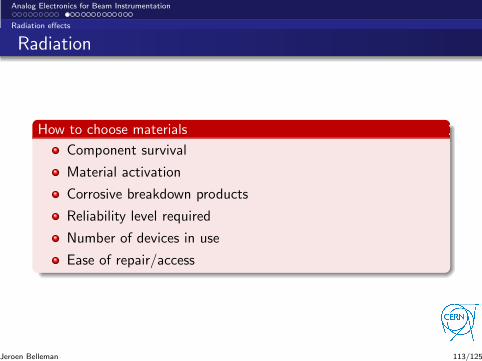
Radiation
How to choose materials
Component survival
Material activation
Corrosive breakdown products
Reliability level required
Number of devices in use
Ease of repair/access
Jeroen Belleman 113/125
Analog Electronics for Beam Instrumentation
Radiation effects
Radiation
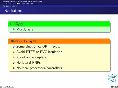
<10Gy/y
Mostly safe
10Gy/y - 1k Gy/y
Some electronics OK, maybe.
Avoid PTFE or PVC insulation
Avoid opto-couplers
No lateral PNPs
No local processors/controllers
Jeroen Belleman 114/125
Analog Electronics for Beam Instrumentation
Radiation effects
Radiation
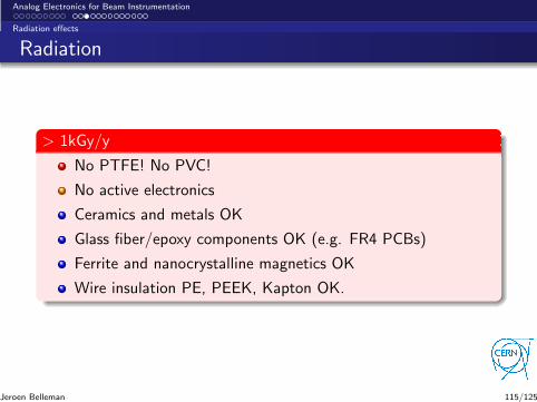
> 1kGy/y
No PTFE! No PVC!
No active electronics
Ceramics and metals OK
Glass fiber/epoxy components OK (e.g. FR4 PCBs)
Ferrite and nanocrystalline magnetics OK
Wire insulation PE, PEEK, Kapton OK.
Jeroen Belleman 115/125
Analog Electronics for Beam Instrumentation
Radiation effects
Radiation tolerant electronic design
The effects depend strongly on manufacturing details likegeometry or doping profiles
Even if some parameters go outside the specified range, thisdoesn’t imply that a component is suddenly useless.
’Equivalent’ devices of different makes may fare verydifferently. This may even happen for different lots of thesame make!
You can’t know for sure if you haven’t done the measurement
Jeroen Belleman 116/125
Analog Electronics for Beam Instrumentation
Radiation effects
Radiation damage to...
Bipolar transistors
Creation of recombination centers in the base
Reduction of hFE at low currents (IC < 100µA)
Design to tolerate wide variation in hFE
Use largish standing currents
Jeroen Belleman 117/125
Analog Electronics for Beam Instrumentation
Radiation effects
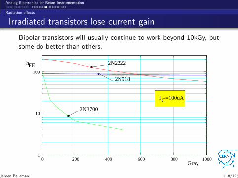
Irradiated transistors lose current gain
Bipolar transistors will usually continue to work beyond 10kGy, butsome do better than others.
Gray
hFE 2N2222
2N918
2N3700
CI =100uA
1
10
100
0 200 400 600 800 1000
Jeroen Belleman 118/125
Analog Electronics for Beam Instrumentation
Radiation effects
Radiation damage to...
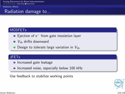
MOSFETs
Ejection of e− from gate insulation layer
Vth drifts downward
Design to tolerate large variation in Vth
JFETs
Increased gate leakage
Increased noise, especially below 100 kHz
Use feedback to stabilize working points
Jeroen Belleman 119/125
Analog Electronics for Beam Instrumentation
Radiation effects
Radiation damage to...
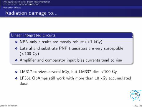
Linear integrated circuits
NPN-only circuits are mostly robust (>1 kGy)
Lateral and substrate PNP transistors are very susceptible(<100 Gy)
Amplifier and comparator input bias currents tend to rise
LM317 survives several kGy, but LM337 dies <100 Gy
LF351 OpAmps still work with more than 10 kGy accumulateddose.
Jeroen Belleman 120/125
Analog Electronics for Beam Instrumentation
Radiation effects
Radiation damage to...
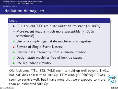
Logic
ECL and old TTL are quite radiation resistant (> 1kGy)
More recent logic is much more susceptible (< 30Gysometimes!)
Use only simple logic, state machines and registers
Beware of Single Event Upsets:
Rewrite data frequently from a remote location
Design state machines free of lock-up states
Use redundant circuitry
Old-fashioned TTL, 74S, 74LS seem to hold up well beyond 1 kGy,but 74F dies at less than 100 Gy. EPM7064 (EEPROM) FPGAsseem to survive well, but I have none that were exposed to morethan an estimated 500 Gy.
Jeroen Belleman 121/125
Analog Electronics for Beam Instrumentation
Radiation effects
Something will break/drift/change
Whether a device is operational or not depends much on how itscomponents are used. If correct operation relies on a parameterthat happens to drift under irradiation, your circuit dies early.
Allow for parameter drift
Allow for large changes in bias/leakage currents, VT , hFE
Avoid very high impedances
Use largish standing currents
Avoid ICs containing lateral or substrate PNP transistors
Jeroen Belleman 122/125
Analog Electronics for Beam Instrumentation
Radiation effects
Defensive Design
Try to confine damage
Remote power supplies (Easy to clear latch-ups, too!)
Split power distribution
Fold-back current limiting, PTC or PolyFuse
Insert sense resistors in power supply connections
Jeroen Belleman 123/125
Analog Electronics for Beam Instrumentation
Radiation effects
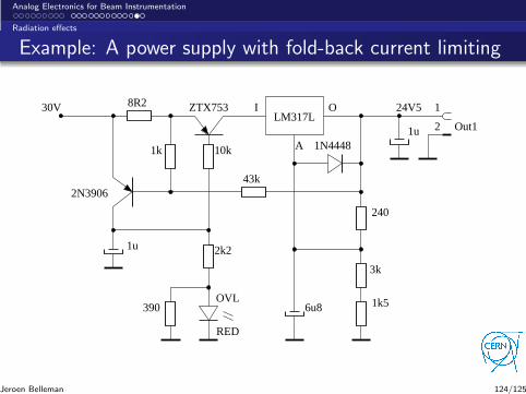
Example: A power supply with fold-back current limiting
LM317L
A
I O30V 24V5 1
2
2N3906
ZTX7538R2
1k 10k
43k
2k21u
OVL390
1N4448
6u8
240
3k
1k5
1u Out1
RED
Jeroen Belleman 124/125
Analog Electronics for Beam Instrumentation
Radiation effects
Thank you
Jeroen Belleman 125/125


