Analysing the drainage system using epa swmm 5.1 (study ...

http://dx.doi.org/10.33021/jenv.v5i2.1234 | 136

Analysing the drainage system using epa swmm 5.1 (study case: jababeka ii industrial, cikarang baru, bekasi regency)

Kezia Kusumaningtyas1*, Yunita Ismail1

1 Environmental Engineering, Engineering Program, President University Bekasi, 17530, Indonesia

Manuscript History

Received 15-09-2020 Revised 17-10-2020 Accepted 11-12-2020 Available online 15-12-2020

Abstract. Due to the data in 2030, the urban growth in developed countries is 83%, and developing countries is 53%. Jababeka II Industrial Estate is one of the urban industrialization located at Bekasi Regency. In its development, the consideration of drainage facilities is one thing that needs. Because with its function as a channel that carries runoff water to rivers/lakes/reservoirs to avoid flooding. Objectives: This study aimed to know the existing condition of the drainage system and the water balances in the form of runoff in Jababeka II Industrial Estate by the simulation of SWMM 5.1. Method and results: The process of this research used a quantitative method, and the data collection method used secondary data, include the information from existing drainage system with precipitation event in 12 years (2009-2020) are obtained from the WTP Jababeka Residential, drainage dimension, and masterplan of Jababeka II. To calculate rainfall planned used a fifth-year return period based, it's on the city's classification under study. The probability distribution method uses Log-Pearson III with a planned rainfall of 128.22 mm/d and the highest rainfall intensity of 54 mm. Based on the simulation results, it was found that the Jababeka II Industrial Estate contained puddles in several channels. The peak was at the 3rd hour of the simulation, which were 19 channels. It's influenced by the type of soil that is quickly saturated. Conclusion: The simulation of the existing condition at Jababeka II has the highest runoff at the 2nd hour of simulation, and floods occurred in 19 channels. It's affected by the impermeable sub-areas. The water balance result is the amount of precipitation 128.22 mm with the intensity is 54mm due to 5 years of forecasting, thus producing the outflow is 128.511 mm. Therefore the number of continuity errors of a surface is -0.227%.

Keywords

flooding; swmm 5.1; drainage; rainfall

* Corresponding author: [email protected]

Vol. 05, No. 02, pp. 136-155, December, 2020


1 Introduction

Human activities significantly disrupt the natural hydrological cycle's quantitative

and qualitative parameters. The statistics data are shown data 83% of developed

worlds and 53% of developing societies predicted to live by 2030 in urban areas.

Urban growth continues to occur in developing countries on broad spatial scales,

with whole cities often built in a short time [1]. This change affects the function of

the land where the water absorption area is reduced. The waterways' number and

dimensions changed so that water infiltration reduces, and flooding is commonly

occurring [2]. The UNESCO Press Paris in 1974 has mentioned the industrialization

include in urbanization [3]. It can be considered human activities involving changes

in land tenure and land use resulting from rural land conversion to industrial use

and urban, suburban, and industrial communities. Surface runoff directly can

convert from more than 40% of rainfall in urban areas with more than 50% of

impervious surfaces 4]. Thus, a drainage system must be supported to prevent

flooding due to flow exceeding the channel capacity.

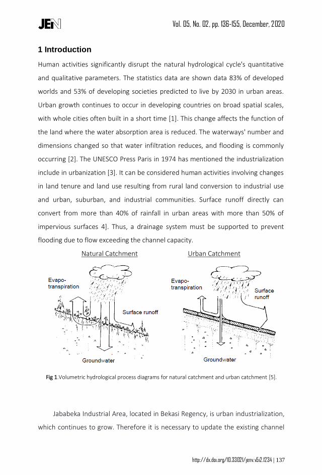
Natural Catchment Urban Catchment

Fig 1.Volumetric hydrological process diagrams for natural catchment and urban catchment [5].

Jababeka Industrial Area, located in Bekasi Regency, is urban industrialization,

which continues to grow. Therefore it is necessary to update the existing channel



system periodically. According to Urban Cikarang news, Jababeka II Industrial

Estate are frequent annual floods occur. The worst floods happened at the

beginning of 2020, where floods were inundated as high as 20 – 150cm [6].

SWMM 5.1 is an application from the US EPA, which mainly consists of

hydraulic and hydrology components that are very easy to use for the community

to choose most often used by the professionals to do flood modeling on drainage

channels. The runoff component of SWMM 5.1 operates on a collection of

subcatchment areas that receive precipitation and generate runoff and pollutant

loads. It transports through the channels ended up in storage/ treatment/ any

outfall devices depend on the needed. SWMM 5.1 can track the quantity and

quality of runoff generated within each subcatchment. The flow rate, flow depth,

and water quality in each pipe and channel during the simulation period comprised

multiple time steps.

This study analyzes the drainage channels in the Jababeka II Industrial Estate

at a time of maximum rainfall for the last 12 years. Thus, this research has two

purposes knowing the Jababeka II Industrial Estate water balances in the form of

runoff during the simulation and knowing the flood occurred in the existing

condition of drainage system using a simulation of SWMM 5.1.

2 Method

2.1 Research Location

The research was carried out from May to July 2020 during the dry season, located

at Jababeka II Industrial Estate, Cikarang Baru, Bekasi Regency (Figure 2). The

drainage system is used to collect rainwater and go to Cilemahabang River. The

channel's location is along the shoulder side of the road with several dimensions

that depend on the elevations.



Fig 2.The area of research location, Jababeka II Industrial Estate

2.2 Population and Sample

Population and sample are an essential part of a study where a community is a unit

of individuals or subjects in the area and time with a certain quality. The research

sample is part of the people used as the research subject as a representative of the

population [15]. In this study, the community is the drainage system from the

entire Jababeka Industrial Estate. At the same time, the sample used is the

drainage system in the Jababeka II Industrial Estate with a maximum daily rainfall

for 12 years, 2009 – 2020, as measured in the sample. Sampling using the

purposive sampling method or judgment sampling is the choice of participants who

deliberate because of the participants' quality and criteria. It's a non-random

technique that does not require an underlying theory or some participants but is

based on the researcher's sample criteria to achieve a specific goal [14]. Based on

this study's standards, the sample taken was determined by the frequent flooding

in the Jababeka Industrial Area and the maximum rainfall over the last ten years.



2.3 Tools and Materials

This study uses secondary data collection methods, which are collected from

Jababeka WTP Residential. They are channel dimension, the water flow direction,

topographic maps, masterplan of Jababeka II Industrial Estate drainage system, and

the daily rainfall intensity data from 2009 – 2020. The tools used during this

research were a laptop, stationery, calculator, Google Earth software, TCX

Converter, Quikgrid, QGis, AutoCad, and SWMM 5.1.

2.4 Research Procedure

In the research procedure, there are several steps to get the data. They are

frequency analysis of hydrological data, rainfall distribution, discharge channel

capacity calculation, and the % impervious and %pervious [16]. The frequency

analysis of hydrological data is the value of rainfall planned or equal to the

definition of maximum probability of rainfall intensity with forecasting in the next

few years, where it depends on the requirement. Then the result will be times with

rainfall distribution according to the previous research. And the final product will

become the time series. Continue to calculate the discharge capacity using

manning’s equation.

After getting the time series and the flowrate of discharge capacity,

determine the %impervious and %pervious.

Below are the following data processing procedures were applied:

a. Frequency Analysis of Hydrological Data

i. Frequency Distribution Selection

This distribution has four types, are Normal Distribution, Log-Normal

Distribution, Gumbel Distribution, and Log-Pearson III Distribution, which were

commonly used for hydrology [17]. The aim to determine whether the choice

of the frequency distribution method used can be accepted or rejected based

on the frequency analysis of statistics parameter tests, which are skewness

coefficient (Cs) and kurtosis coefficient (Ck). The distribution selected for this

research is Log Pearson III that complied with the criteria.



ii. Testing the Suitability of Frequency Distribution

The frequency distribution that set should be tested using the suitability of

frequency distribution testing. There are two distribution tests: the first is the

chi-square test (1) and Smirnov-Kolmogorov (2) [18].

𝑋2ℎ = ∑ (𝑂𝑖−𝐸𝑖)3𝑄

𝑖=1

𝐸𝑖 (1)

𝐷 = 𝑚𝑎𝑥𝑖𝑚𝑢𝑚 |𝐹𝑠(𝑋) − 𝐹𝑡(𝑋)| (2)

b. Rainfall intensity

The planed rainfall value can be calculated after determining the frequency

distribution to be used. Nevertheless, SWMM 5.1 claims that the rainfall value is

a constant value that uses time series to continue over a given recording period

for rainfall measurements. So what is calculated in the other SWMM 5.1 time-

series is between the reported values [11]. In this case, the rain distribution

value derived from the literature can be used as a time series for modeling [13].

c. Discharge Channel Capacity

Data needed for the addition of discharge outflow (initial flow) from the runoff

into the channel uses Manning’s equation (3) [8]:

V = 1

n x R

2

3 x S1

2 (3)

Q = A x V (4)

Where :

Q = flow rate (m3/s)

A = channel cross-section area (m2)

V = velocity (m/s)

R = hydraulic radius (cross-section area divided by wetted

perimeter) (m)

S = slope of the channel at the point of measurement (%)

d. Determining the %impervious and %pervious



To determine the percent of impervious and pervious values, analyze from the

location map. As mentioned from SWMM 5.1 Modul, subcatchment is an area

of land comprising a mixture of pervious and impervious layers, the runoff of

which drains to a specific outlet site. Surface runoff may permeate but not

through the impermeable sub-area into the pervious sub-area's upper soil zone.

Impermeable areas are themselves divided into two sub-areas-one that

includes depression storage and one that does not. Storage depressions are

used for water reservoirs in the field that are permeable to infiltration in

subsequent periods. Depression storage is rainwater that stagnates in

impermeable soil until it evaporates. The percentage of impervious areas inside

the subcatchment is except depressions in storage [11]. Equation numbers 5

and 6 are the formula to get impermeable and permeate percentage values.

%impervious = 100% x (impervious area

total area−LID area) (5)

%pervious = 100 − %impervious (6)

The method of infiltration calculation used for modeling is the Horton

method. Based on the interpolation of observations, the infiltration decreases

exponentially from the initial maximum to the minimum rate during extended

rainfall. The required parameters include the maximum and minimum infiltration

rate, the decay coefficient, which describes how fast the rate of decay over time,

and the time it takes for the saturated soil to dry again completely. After ensuring

that all the required data is entered into the modeling process, the modeling can

be started [11].



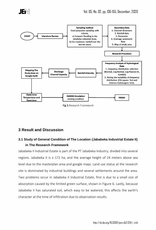
Fig 3.Research Framework

3 Result and Discussion

3.1 Study of General Condition of The Location (Jababeka Industrial Estate II)

in The Research Framework

Jababeka II Industrial Estate is part of the PT Jababeka Industry, divided into several

regions. Jababeka II is ± 172 ha, and the average height of 24 meters above sea

level due to the masterplan area and google maps. Land use status at the research

site is dominated by industrial buildings and several settlements around the area.

Two problems occur in Jababeka II Industrial Estate, first is due to a small size of

absorption caused by the limited green surface, shown in Figure 6. Lastly, because

Jababeka II has saturated soil, which easy to be watered, this affects the earth's

character at the time of infiltration due to observation results.



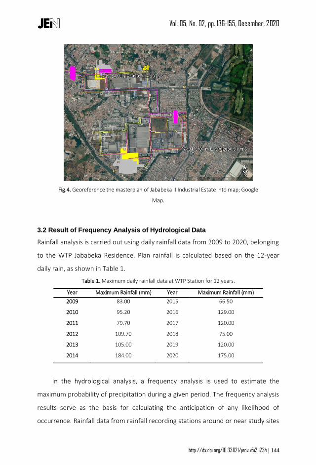
Fig.4. Georeference the masterplan of Jababeka II Industrial Estate into map; Google

Map.

3.2 Result of Frequency Analysis of Hydrological Data

Rainfall analysis is carried out using daily rainfall data from 2009 to 2020, belonging

to the WTP Jababeka Residence. Plan rainfall is calculated based on the 12-year

daily rain, as shown in Table 1.

Table 1. Maximum daily rainfall data at WTP Station for 12 years.

Year Maximum Rainfall (mm) Year Maximum Rainfall (mm)

2009 83.00 2015 66.50

2010 95.20 2016 129.00

2011 79.70 2017 120.00

2012 109.70 2018 75.00

2013 105.00 2019 120.00

2014 184.00 2020 175.00

In the hydrological analysis, a frequency analysis is used to estimate the

maximum probability of precipitation during a given period. The frequency analysis

results serve as the basis for calculating the anticipation of any likelihood of

occurrence. Rainfall data from rainfall recording stations around or near study sites



are hydrological data required for drainage design [12]. Frequency analysis can be

carried out using four probability distribution methods shown in Table 2 along with

2, 5, 10, and 50-year rainfall and return period.

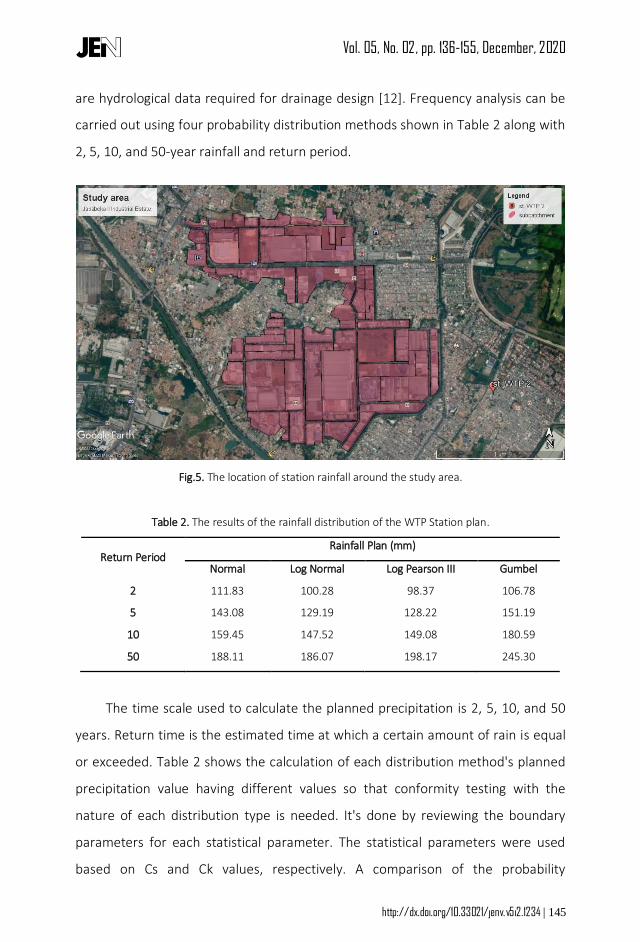
Fig.5. The location of station rainfall around the study area.

Table 2. The results of the rainfall distribution of the WTP Station plan.

Return Period Rainfall Plan (mm)

Normal Log Normal Log Pearson III Gumbel

2 111.83 100.28 98.37 106.78

5 143.08 129.19 128.22 151.19

10 159.45 147.52 149.08 180.59

50 188.11 186.07 198.17 245.30

The time scale used to calculate the planned precipitation is 2, 5, 10, and 50

years. Return time is the estimated time at which a certain amount of rain is equal

or exceeded. Table 2 shows the calculation of each distribution method's planned

precipitation value having different values so that conformity testing with the

nature of each distribution type is needed. It's done by reviewing the boundary

parameters for each statistical parameter. The statistical parameters were used

based on Cs and Ck values, respectively. A comparison of the probability



distribution parameters can be found in Table 3. The results of the calculation of

the Chi-Square Log Pearson III distribution are shown in Table 4.

Table 3. The result of the statistic parameters [9].

No Frequency

Distribution Types Cs Ck

Criteria

Cs Ck

1 Normal 0.91 0.16 Cs ≈ 0 Ck ≈ 3

2 Log Normal 0.68 0.43 Cs = 0.43 Ck = 3.33

3 Gumbel 0.91 0.16 Cs = 1.14 Ck = 5.4

4 Log Pearson III 0.68 0.43 Apart from the above

The chi-square test requirements can be accepted if the X2 value in the

calculation results is less than the X2 value in the Chi-squared test table. Based on

the products shown in Table 4, the resulting X2 value is 3.83, while the Chi-Square

X2 test table is 5.991. It was concluded that the method of distribution of the

Pearson III Log was used. The precipitation value used in the simulation shall be

128.22 mm/d with a return based on Regulation No 12/PRT/M/14 of the Minister

of Public Works concerning the implementation of the 5-year urban drainage

system [10].

Table 4. Chi-Square Log Pearson III Distribution testing results.

Class Interval Oi Ei Oi - Ei (Oi – Ei)2 (Oi – Ei)2/Ei

1 51.81 - 81.19 3 2.4 0.6 0.36 0.15

2 81.19 - 110.57 4 2.4 1.6 2.56 1.07

3 110.57 - 139.94 3 2.4 0.6 0.36 0.15

4 139.94 - 169.3 0 2.4 -2.4 5.76 2.40

5 169.3 - 198.68 2 2.4 -0.4 0.016 0.07

Total X2 3.83

3.3 Result of Rainfall Intensity Calculation

The hourly rainfall distribution was used based on the distribution obtained by Fajri

(2009)[13], as shown in Table 5. The value of rain distribution is used as a bulk time



series plan for SWMM 5.1 model. The first hour has the highest percentage of the

peak hour simulation to have a significant runoff potential.

Table 5. Distribution of the intensity of precipitation event

Time (h) 0 1 2 3

Rainfall distribution (%) 0 42.35 39.51 18.14

Rainfall plan (mm) 0 54 51 23

3.4 Result of Hydraulic Analysis on Existing Channels

The hydraulic analysis is carried out to determine whether the planned drainage

system is following the requirements. This analysis includes the calculation of

existing channel capacity and channel planning. Table 6 shows the results of the

hydraulic study.

Table 6. Result of the analysis of discharge existing channel capacity

Name of

channel

Area

(A)

m2

Wetted

Perimeter

(P)

m

Hydraulic

Radius

(R)

m

Velocity

(V)

m/s

Discharge Existing

Channels

(Qs)

m3/s

C1 1.51 3.65 0.414 0.490 2.67

C2 1.51 3.65 0.414 0.490 2.67

C3 1.90 3.98 0.478 0.540 3.699

C4 2.16 4.22 0.513 0.565 4.41

C5 2.13 4.18 0.509 0.563 4.32

The following Table 7 presents the results of the analysis of hydraulic

discharge and hydrological discharge for the five year return period. The hydraulic

analysis results are accepted because the hydrological capacity is smaller than the

hydraulic capacity.

Table 7. The analysis of channel planning capacity

Name of

channel

Qhydrology

Discharge Existing Channels

(Qs)

Qhydrology <

Qhydraulic

Return

period m3/s m3/s m/s



C1 5 0.092 2.67 accepted

C2 5 0.101 2.67 accepted

C3 5 0.180 3.699 accepted

C4 5 0.101 4.41 accepted

C5 5 0.246 4.32 accepted

3.5 %Impervious and %Previous

Table 8 shows the subcatchment parameter values, which consist of areas of

subcatchment, length, and size. This width came from an average of the total

length, percent of the impervious and pervious area. The value of the impervious

percentage depends on the impermeable site on subcatchment. Other than that, it

also represents the result comparing the subcatchment area with impermeable

subarea.

Table 8. Subcatchment parameter modelling data

Name Area

(ha)

Length

(m)

Width

(m)

Pervious

(%)

Impervious

(%)

SUB 1 0.63 180.32 35.87 4.98 95.02

SUB 2 0.68 137.47 38.71 11.79 88.21

SUB 3 1.21 151.24 68.89 71.56 28.44

SUB 4 0.68 110.24 38.71 25.16 74.84

SUB 5 1.65 245.6 93.94 19.92 80.08



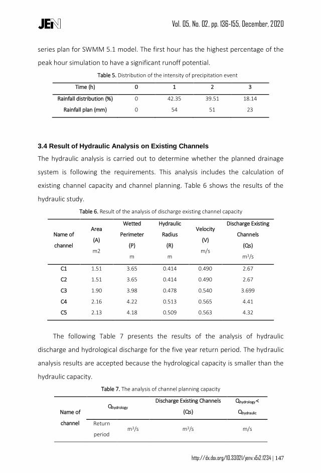
Fig.6. The impervious area condition in subcatchment. (yellow color is impermeable sub-area and

purple color is subctachment area)

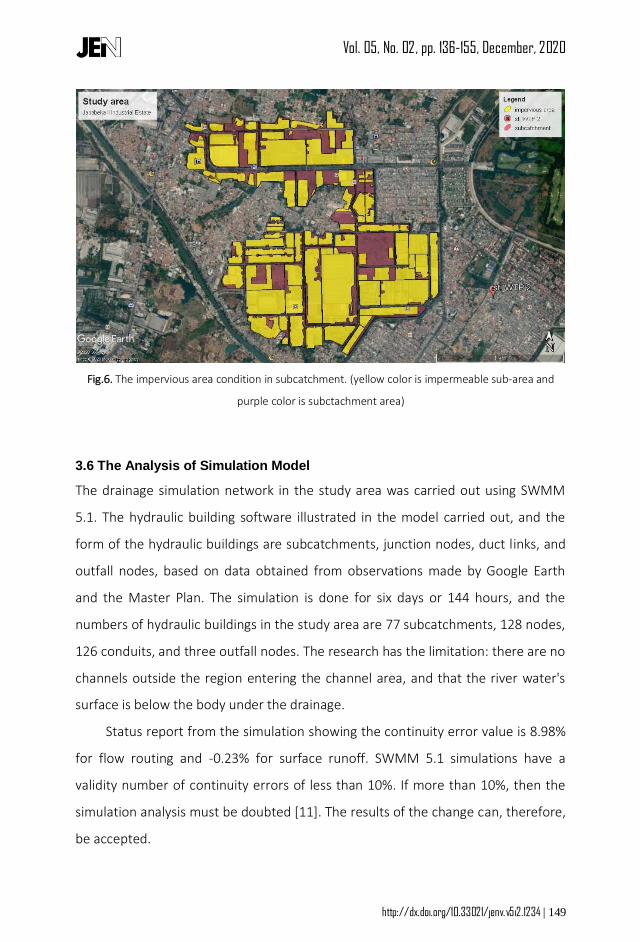
3.6 The Analysis of Simulation Model

The drainage simulation network in the study area was carried out using SWMM

5.1. The hydraulic building software illustrated in the model carried out, and the

form of the hydraulic buildings are subcatchments, junction nodes, duct links, and

outfall nodes, based on data obtained from observations made by Google Earth

and the Master Plan. The simulation is done for six days or 144 hours, and the

numbers of hydraulic buildings in the study area are 77 subcatchments, 128 nodes,

126 conduits, and three outfall nodes. The research has the limitation: there are no

channels outside the region entering the channel area, and that the river water's

surface is below the body under the drainage.

Status report from the simulation showing the continuity error value is 8.98%

for flow routing and -0.23% for surface runoff. SWMM 5.1 simulations have a

validity number of continuity errors of less than 10%. If more than 10%, then the

simulation analysis must be doubted [11]. The results of the change can, therefore,

be accepted.



Fig.7. Simulation of drainage system models and study area flow patterns in the

first hour.

The models and Figure 7 show the results of simulation of Jababeka II

Industrial Estate using SWMM 5.1 on the first hour with the arrow as a direction of

water flow that happened in the channel. The needle has color represent the

drainage condition. Red color means an overflow in the track where the runoff

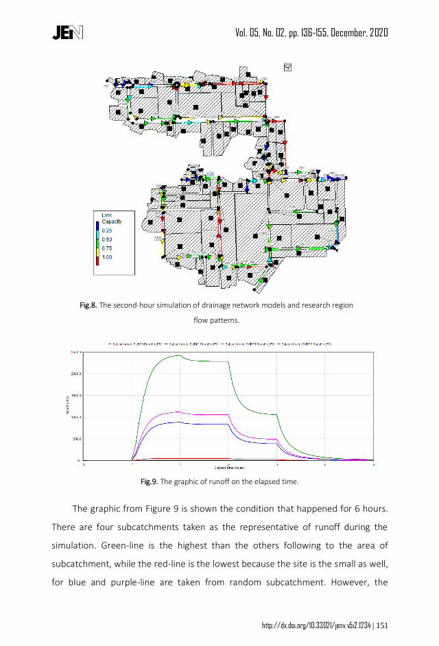
discharge exceeds the channel's discharge capacity. Whereas in Figure 8, there is a

simulation of the second-hour drainage network model. There are additional flood

channels, namely C12, C25, C33, C36, C37, C40, C41, C42, C54, C55, C68, C69, C88,

C96, C97, C103, C114, C115, and C123. As shown in Figure 9, the runoff water will

peak in the second hour. In the time series case, this is influenced by the soil

nature area and the second factor of flooding in which the soil type is saturated. So

that in the first hour, the land is dry. The ground can then absorb rainwater, but in

the next hour, the soil will be saturated and become runoff water.



Fig.8. The second-hour simulation of drainage network models and research region

flow patterns.

Fig.9. The graphic of runoff on the elapsed time.

The graphic from Figure 9 is shown the condition that happened for 6 hours.

There are four subcatchments taken as the representative of runoff during the

simulation. Green-line is the highest than the others following to the area of

subcatchment, while the red-line is the lowest because the site is the small as well,

for blue and purple-line are taken from random subcatchment. However, the



whole four lines have the same graphic shape. Even the area of subcatchments is

different, where it shows that the amount of runoff has a linear relationship with

the subcatchment area.

Fig.10. The condition of C88 profile of channel traffic.

Figure 10 shows the state of the C88 channel flooded due to the amount of

runoff discharge so that the channel's capacity is not enough—the same as in

Figures 6 and 7 for the red channels.

Table 9. The status report of runoff from the simulation

Runoff Quantity Continuity Volume Hectare (m) Depth (mm)

Total precipitation 37.088 128.220

Evaporation loss 0.000 0.000

Infiltration loss 0.315 1.089

Surface runoff 30.078 103.985

Final storage 6.779 23.437

Continuity error (%) -0.227

According to the current condition result, it can be seen that there is an

imbalance in the water balance then resulting in flooding. The water balance of

SWMM 5.1 is interpreted by a percentage of a continuity error, where it represents

the differences between initial storage + total inflow and final storage + total

outflow. Table 9 has shown the status report from simulation results in Jababeka II

Industrial Estate, with the number of precipitation is 128.22 mm. As a result, the



continuity error for surface runoff is -0.227% came from total outflow that consists

of rain rather than divided with total inflow consisting of evaporation, infiltration

loss, and surface runoff, and final storage. The number of precipitation came from

the rainfall planned (mm), which is the water source that enters the study area.

Meanwhile, the evaporation, infiltration loss, and surface runoff are the sources of

runoff water.

4 Conclusion

The simulation carried out in Jababeka II Industrial Estate using SWMM 5.1, which

showed that the highest runoff value occurs at the 2nd hour, which is influenced

by a limited green surface. The total numbers of a channel that floods occurred

during the 2nd hour are 19 channels with different channel sizes affected by land

elevation. According to the water balances of rainfall planned, 128.22 mm, which is

rainfall intensity 54 mm due to 5 years forecasting, and total outflow is 128.511

mm resulting continuity error of surface runoff is -0.227%.

5 Acknowledgment

Thank you to Dr. Ir. Yunita Ismail Masjud, M.Sc., who helped and guided through

finish this research. As well as the WTP Jababeka Residence, who helped collect all

data needed during this research. And also like to thank Mr. Rijal Hakiki S.S.T., M.T.,

which helped to do simulation modeling that could work well.



6 References

[1] C. R. Jacobson, “The Concept of Sustainable Urban Water Management.,” Elsevier, pp.

1438–1448, 2011.

[2] R. Wirosoedarmo, J. B. Rahadi, A. Tunggul S.H, and N. S. M. Andi, “Evaluasi Kinerja

Saluran Drainase Pemukiman dengan Menggunakan Perangkat Lunak EPA SWMM 5.1

(Studi Kasus Perumahan Sawojajar Kota Malang, Indonesia),” Journal Sains dan

Teknologi Pangan, pp. 246–247, Oct. 2017.

[3] M. Mcpherson, “Hydrological effects of urbanization Report of the Sub-group on the

Effects of Urbanization on the Hydrological Environment, of the Co-ordinating Council

of the International Hydrological Decade Prepared under the chairmanship of,” The

Unesco Press, Paris, 1974.

[4] L. Yao, L. Chen, W. Wei, and R. Sun, “Potential reduction in urban runoff by green

spaces in Beijing: A scenario analysis,” Urban Forestry & Urban Greening, vol. 14, no.

2, pp. 300–308, 2015.

[5] M. Sokac, “Water Balance in Urban Areas,” IOP Conference Series: Materials Science

and Engineering, vol. 471, p. 042028, Feb. 2019.

[6] “Ketika Jababeka Terendam Banjir,” www.urbancikarang.com, 2014. [Online].

Available: http://www.urbancikarang.com/v2/page.php?halaman=Ketika-Jababeka-

Terendam-Banjir#.XyLmmigzbRp. [Accessed: 30-Jul-2020].

[7] M. Niazi et al., “Storm Water Management Model: Performance Review and Gap

Analysis,” Journal of Sustainable Water in the Built Environment, vol. 3, no. 2, p.

04017002, May 2017.

[8] I. Dorojatun, “Evaluasi Saluran Drainase di Perumahan Taman Aster Cikaranag Barat

Kabupaten Bekasi dengan Menggunakan EPA SWMM 5.1,” Thesis, Institusi Pertanian

Bogor, 2017.

[9] L. Kartiko and R. S. B. Waspodo, “Analisis Kapasitas Saluran Drainase Menggunakan

Program SWMM 5.1 di Perumahan Tasmania Bogor, Jawa Barat,” Jurnal Teknik Sipil

dan Lingkungan, vol. 3, no. 3, pp. 133–148, Dec. 2018.

[10] Peraturan Menteri Pekerjaan Umum Nomor 12/PRT/M/2014 tentang

Penyelenggaraan Sistem Drainase.

[11] L. A. Rossman, Storm Water Management Model User’s Manual Version 5.1. Cincinati,

Ohio: US Environmental Protection Agent, 2015, pp. 1–353.



[12] E. Widodo and D. Ningrum, “Evaluasi SIstem Jaringan Drainase Permukiman Soekarno

Hatta Kota Malang dan Penanganannya,” Jurnal Ilmu-Ilmu Teknik, vol. 11, no. 3, 2015.

[13] I. Fajri, ‘Membuat Pola Sebaran Hujan dan Isohyet pada DAS Ciliwung – Cisadane,”

Thesis, Universitas Indonesia, 2009.

[14] I. Etikan, “Comparison of Convenience Sampling and Purposive Sampling,” American Journal of Theoretical and Applied Statistics, vol. 5, no. 1, p. 1, 2016.

[15] H. Taherdoost, “Sampling Methods in Research Methodology; How to Choose a

Sample Technique for Reseach,” International Journal of academic Research in

Management (IJARM), vol. 5, no. 2, pp. 18–27, Jan. 2016.

[16] N. Augusta, “Evaluasi Saluran Drainase dengan Menggunakan Program SWMM 5.1 di

Perumahan Villa Ratu Endah, Bogor, Jawa Barat,” Thesis, Institut Pertanian Bogor,

2017.

[17] Hudhiyantoro and F. Saves, “Potensi Penerapan Ecodrainage di Desa Sumberejo

Kecamatan Pakal Kota Surabaya,” Jurnal Teknik Sipil, vol. 1, no. 5, Mar. 2019.

[18] M. Suprapto, A. Y. Mutaqin, and A. S. Prilbista, “ANALISIS SISTEM DRAINASE UNTUK

PENANGANAN GENANGAN DI KECAMATAN MAGETAN BAGIAN UTARA,” Matriks

Teknik Sipil, vol. 6, no. 1, Mar. 2018.

Date post:	25-Feb-2022
Category:	Documents
Upload:	others
View:	4 times
Download:	0 times

Analysing the drainage system using epa swmm 5.1 (study ...

Documents