Analysing the Impact of Trade Preferences in Gravity Models. Does Aggregation Matter? Maria Rosaria Agostino, Francesco Aiello and Paola Cardamone (University of Calabria, Italy)

Working Paper 07/4 TRADEAG is a Specific Targeted Research Project financed by the European Commission within its VI Research Framework. Information about the Project, the partners involved and its outputs can be found at

University of Dublin Trinity College

http://www.tradeag.eu

Analysing the Impact of Trade Preferences in Gravity Models. Does Aggregation Matter?1

Maria Rosaria Agostino, Francesco Aiello, Paola Cardamone (agostino@unical.it – f.aiello@unical.it – p.cardamone@unical.it)

UUUnnniiivvveeerrrsssiii tttyyy ooofff CCCaaalllaaabbbrrriiiaaa DDDeeepppaaarrrtttmmmeeennnttt ooofff EEEcccooonnnooommmiiicccsss aaannnddd SSStttaaattt iiisssttt iiicccsss

III---888777000333666 AAArrrcccaaavvvaaacccaaatttaaa dddiii RRReeennndddeee (((CCCSSS))) --- III tttaaalllyyy

Abstract. There are two sources of bias in the existing gravity equations used to assess the impact of non-reciprocal preferential trade policies (NRPTPs). The main inconsistency comes from the use of aggregate export flows at country level to analyse the effects of trade preferences which, by contrast, apply at product level. The second source of bias is that the literature does not deal with the main econometric issues which are likely to be present when a gravity equation is estimated. This paper discusses the first problem using evidence based on three levels of data aggregation (total exports, total agricultural exports and 2-digit). Furthermore, the estimation methods take into account the unobservable country heterogeneity as well as the endogeneity of trade preferences and the potential selection bias which zero-trade values pose. We consider all NRPTPs granted by 8 major OECD countries to exports from developing countries over the period 1995-2003. We find two key results. First of all we show that the impact of NRPTPs on total exports is positive, whatever the estimator. This means that, other things being equal, the national exports to the preference-giving country of a preferred country are higher than those of a non-preferred country. Secondly, when the analysis is conducted at 2-digit level, it emerges that the preference premium is very high in many 2-digit sectors, whatever the preferential treatment (GSP and/or other preferences). This finding stands in contrast with the result obtained when total exports are considered, which places the preference gain at lower values.

1. Introduction Over the last decade many studies have employed the gravity model to evaluate the impact of non-reciprocal preferential trade policies (hereafter NRPTPs) on the export performance of developing countries. The aim of this paper is to provide new empirical evidence in this area of research.

A NRPTP is a concession granted to developing countries by a developed country on a unilateral basis, that is without reciprocal preferences for the donor’s exports. Beneficiary countries have access to the donor’s market duty-free or with a preferential tariff and, as a result of this special treatment, an increase in their exports

1 Address correspondence to: Francesco Aiello, University of Calabria, Department of Economics and

Statistics, I-87036 Arcavacata di Rende (CS) Italy. The authors acknowledge the very valuable contribution made by Giovanni Anania in identifying the research issues and in helping improving previous versions of the paper. They are also indebted to Alan Matthews, Anne Celie Disdier, Fernanda Ricotta and Anastasia Semykina for useful comments on an earlier version. Financial support received by the European Commission (Specific Targets Research Project, “Agricultural Trade Agreements (TRADEAG)” research project. Contract no. 513666) is gratefully acknowledged.

- 2 -

towards the preference-giving country is expected to occur. The main active NRPTP is the Generalized System of Preferences (GSP) recommended by UNCTAD in 1968 and implemented by major developed countries since the early ’70s. Today, under the GSP, the exports of selected products of about 150 developing countries benefit from reduced tariffs when entering donor markets. Apart from the GSP, virtually all developing countries are members of at least another preferential trade scheme granted by a developed country to favour exports originating from developing countries.2

The gravitational approach offers a framework for assessing whether NRPTPs affect bilateral trade flows between beneficiaries and donors. In its simplest form, the gravity model posits that the normal level of trade is positively affected by the economic mass of the trading countries (richer and larger nations both export and import more) and negatively influenced by the geographical distance between them. The “normal” level of trade is the average level of trade in a world free of trade barriers, preferential treatments and trade agreements. Such a “normal” level is defined as the counterfactual. When developed countries grant special treatment to exports from developing countries, they introduce a disturbance into the model that defines the counterfactual and, hence, ceteris paribus, deviations from the “normal” level of trade are interpretable as the effect of the preferential policy.

Although gravity models have a long and well-established history in the explanation of trade, they have seldom been used to study the impact of NRPTPs. A few exceptions are the papers by Oguledo and Macphee (1994), Nouve and Staatz (2003), Persson and Wilhelmsson (2005), Nilsson (2002, 2005), Verdeja (2006), Lederman and Özden (2004), Subramanian and Wei (2005) and Goldstein et al. (2003).

These papers share three common practices. The first is that they evaluate the impact of preferences granted by one or two donors only, which usually are the EU and/or the US. The second common denominator is their focus on total exports from the beneficiary to the donor countries. Lastly, they model NRPTPs by augmenting the gravity model with a preference dummy. Hence, in all these studies, when the estimated coefficient of the preference dummy is significant and positive, it is said that the average level of total exports from a preferred country to the donor is higher than the mean of total exports of a non-preferred country.

We argue that these methodological choices are misleading if the scope of the analysis is to evaluate the impact of a specific trade policy – the preferential trade preference - that is conceived to be applied at product level. Specifically, the main motivation for this study lies in the belief that the objective of NRPTRs is not to affect total trade of the beneficiaries, but to alter the incentives for developing countries to export more in specific sectors in which preferences are granted. Hence, evidence based on disaggregated data is needed to assess the impact of NRPTPs.3 We use data at 2-

2 Another form of trade preference is represented by regional free-trade areas between developed and

developing countries. However, this involves reciprocal preferences and does not constitute an example of trade preferences for developing countries in a strict sense.

3 It is worth underlining that, in general, the “aggregation bias” would be limited if preferences were measured more precisely than by means of dichotomous variables. In other words, it is the combination of aggregate data with the use of dummies that we question, and not the aggregation per se. The main caveat is related to the fact that partial coverage of trade preferences is disregarded using dummy variables and aggregate data. Conversely, there should be no aggregation bias if the value of the

- 3 -

digit level as an attempt to verify the robustness of the results passing from a higher to a lower aggregation of data.

In light of these considerations, the key hypothesis of the paper is that, when overall exports are considered, the impact of NRPTPs might be underestimated. Indeed, if the export shares of sectors that account for a higher margin of preference are small, then the aggregate flow probably does not change enough for the impact of NRPTPs to be picked up in the econometric analysis.5

In order to empirically test our hypothesis we follow the literature with regards the framework of analysis to be used, that is the gravity model, and the use of the preference dummies.6 This allows us to compare our outcomes with those obtained by others. However, we introduce what we believe are three relevant innovations.

First of all, we consider the following three levels of data aggregation: total exports, total agricultural exports and export flows for ten groups of agricultural products at 2-digit level. Agricultural trade has been chosen as the focus of the analysis because of the higher margin of trade preferences enjoyed by developing countries in agriculture with respect to other sectors. We expect that the regressions run at each level of data aggregation will yield different values for the coefficients associated with the preference dummy. In other words, when focusing on sectors enjoying a large margin of preferences, we expect that the estimates are higher than those obtained using

preferences was measured correctly (for example, by weighting the dummy 1 by the proportion of overall trade which actually received the preference).

5 If our hypothesis were true then we could argue that the pre-existing research on the impact of NRPTPs should be interpreted with extreme caution. Indeed, in the debate on the advantages which trade liberalisation might bring to developing countries, it is necessary to investigate the effectiveness of trade preferences. If trade preferences are found to be ineffective then, other things being fixed, the gains for developing countries will remain virtually unchanged when moving from the current protected trade regime to a scenario of full liberalisation. On the other hand, if preferential policies positively affect the export flows of preferred products, then a generalised reduction in tariffs will induce high losses for developing countries due to the erosion of trade preferences.

6 The only reason why we follow the dummy variable approach is that the paper focuses on the aggregation bias, maintaining the method used by others to measure the preferential treatment. However, in carrying out our work, we bear in mind that the dummy variables do not adequately gauge the margin of preference enjoyed by developing countries. Indeed, they are subject to three main critiques. Firstly, they treat all beneficiaries as a homogenous group. This cancels the variance in the group of beneficiaries and disregards the country heterogeneity due, for example, to the different rate of utilization of preferential margins by developing countries. A further drawback regards the fact that dummy variables do not discern between the different trade policy instruments (Tariffs Rate Quotas/Variable levies, preferential margins, calendar, entry price) that have different effects on export flows. Finally, dummy variables do not distinguish the level of trade preference established under the different schemes. In other words, this approach assumes that the margin of preference enjoyed by developing countries under the GSP is equal to that under another NRPTP. The overcoming of these caveats deserves further attention and is the scope of successive research.

- 4 -

aggregated data. Such differences will be considered as evidence in favour of our hypothesis that aggregation matters and leads the underestimating of the role of NRPTPs. If this is the case, we argue that the conclusions about the effectiveness of NRPTPs should be drawn by looking at regressions run at the most disaggregated level relevant in order to properly distinguish sectors in which preferences are granted from those where preferences are not given.

Secondly, for each level of data aggregation we consider export flows, whatever the country-source, towards the OECD members which grant almost all one-way trade preferences (EU15, USA, Japan, Norway, Switzerland, Australia, Canada and New Zealand). Hence, the set of non-reciprocal preferential trade arrangements analysed in this study is almost exhaustive of all one-way programs granted by developed to developing countries over the period under scrutiny (1995-2003).

Thirdly, we employ a panel data specification of a gravity model which is robust to the presence of unobserved country heterogeneity. Moreover, we address the issue of non-random selection which zero-trade observations pose in the log-linearization of the gravity model and perform a test for the endogeneity of trade preferences. The OLS estimates are also presented to allow for comparison.

This empirical strategy allows us to revisit two prominent lines of research in the application of the gravity approach. We use as a bench mark the results obtained at total export level estimated using a method (OLS) that exposes the outcomes to omitted variable, selection and endogeneity bias. We find that eliminating these biases leads to striking changes in results. For example, from OLS regressions it emerges that the total exports of a country eligible for ordinary GSP are 42% higher than those of a non preferred country. Instead, the advantage is 57% when applying Heckman. The difference in the estimation of the preference premium is even larger when we consider all NRPTPs other than GSP: in such a case, the assessment of the extra premium is equal to 103% with OLS and to 142% with Heckman estimator. The second result we provide is partially in line with the expected impact of preference trade policy. Indeed, we show that the estimated impact of NRPTPs in several 2-digit agricultural sectors is higher than that obtained at overall export level.

The paper is structured as follows. Section 2 briefly overviews the related literature, while section 3 describes the gravity model. Section 4 presents data and variables used, whereas section 5 discusses how we treat zero trade values. Sections 6, 7 and 8 present the results obtained by estimating the gravity model though different estimation methods. Section 9 concludes.

2 Related Literature Since the seminal papers by Tinbergen (1962) and Pöyhonen (1963), the gravity equation has been a widely used approach to explain bilateral trade. Typically, the model considers that trade is promoted by the economic size of the trade partners and negatively affected by their geographical distance. Other observable characteristics of each pair of countries (e.g., a common language or a common border) affecting bilateral trade flows can easily be added.

However, the literature that uses gravity equations to specifically assess the impact of NRPTPs in favour of developing countries comprises few contributions, such as the papers by Oguledo and Macphee (1994), Nouve and Staatz (2003), Persson and

- 5 -

Wilhelmsson (2005), Nilsson (2002, 2005) Verdeja (2006), Lederman and Özden (2004), Subramanian and Wei (2005), and Goldstein et al. (2003).7 The impact of the Euro-Mediterranean trade agreements has been analyzed by Amurgo-Pacheco (2006), Pusterla (2007), Gaulier et al. (2004), Garcia-Ảlvarez-Coque and Martì-Selva (2006) and Emlinger et al. (2006). In what follows we briefly present each of these papers highlighting both the methodology used in assessing the impact of NRPTPs and the results obtained.8

Oguledo and Macphee (1994) estimate the effect of an array of discriminatory arrangements (GSP, Lomé, EFTA and Mediterranean) in place in 1976, modelling total exports of 162 countries to 11 major preference-giving countries (EU as one, USA, Japan, Norway, Sweden, Australia, Austria, Canada, New Zealand, Finland and Switzerland). The analysis by Nilsson (2002) compares trade preferences granted by the EU under the GSP scheme and the Lomé Convention from 1973 to 1992. Nouve and Staatz (2003) focus on the impact of the African Growth and Opportunity Act (AGOA) on total agricultural exports from Sub-Saharan African countries (SSA) to the US over the period 1999-2002. Persson and Wilhelmsson (2005) investigate the impact on EU imports of both trade preference schemes and EU enlargements from 1960 to 2002. Nilsson (2005) compares the effect on LDC exports of EU and US preferential trade policies in the period 2001-2003. Verdeja (2006) analyzes the effectiveness of NRPTPs granted by the EU to developing countries over the period 1973-2000, whereas Lederman and Özden (2004) consider US imports in 1997 and 2001. Finally, Subramanian and Wei (2005) and Goldstein et al. (2003) focus on the impact of GSP, using an extensive sample of countries (more than 170) over a very long span period [1948-2001 in Goldstein et al. (2003) and 1950-2000 in Subramanian and Wei, 2005)].

In order to assess the effectiveness of trade preferences, Oguledo and Macphee (1994) use some dummy variables indicating the presence of discriminatory trade agreements and the tariff rates expressed on an ad valorem basis. They point out that, while the tariff variable could be thought of as indicating the trade creation effect of lower tariffs, the dummy may capture the trade diversion effect of the preferences. Their results seem to confirm this hypothesis because both dummy and tariff variables are significant and allow them to conclude that “the tariff variable does not fully reflect the impact of the GSP on imports from beneficiaries” (Oguledo and Macphee 1994, p.

7 We do not survey all the gravity model literature where NRPTPs are used just as controlling variables in

models set up to study other trade issues (i.e. Rose 2003 and 2005). Neither do we consider those papers which investigate the effects of GSP on developing countries total trade (i.e. Rose 2004). This is because we are interested in studying the impact of NRPTPs on export performance, rather than on developing countries trade openness. Besides, as Subramanian and Wei (2005, p. 7) point out, “all theories that underlie a gravity-like specification yield predictions on unidirectional trade rather than total trade”. For a comprehensive review of the papers devoted to assess the impact of preferential trade policies (reciprocal and non reciprocal) using gravity models see Cardamone (2007). Moreover, a detailed survey of the approaches other than the gravity model for evaluating the impact of NRPTPs is provided by Nielsen (2003).

8 We focus on the empirical applications of gravity models. However, many studies provide theoretical explanations for why gravity equations seem to explain trade patterns so well. It is worth noting that these studies derive the gravity equation from very different theories of international trade. A recent influential contribution to the theory of gravity models is the work by Anderson and Wincoop (2004).

- 6 -

119).9 In particular, in the case of EU imports, the negative sign of the tariff variable indicates that lower tariffs do increase EU imports, while the positive value of GSP and Lomè dummies indicates additional effects of preferential schemes.

Nilsson’s (2002) results show a positive and significant impact of EU GSP and the Lomé Convention in all regressions. Nouve and Staatz (2003) find a positive, albeit insignificant, impact of AGOA on agricultural SSA exports to the US. Moreover, their fixed effect model has a very low explanatory power. All these findings are interpreted by the authors as an inconclusive evidence regarding the impact of AGOA.

According to Persson and Wilhelmsson’s (2005) analysis, EU enlargements divert trade, while preferences have a positive impact on the exports of beneficiary countries. Therefore, the authors argue that when a country joins the EU, it will trade less than before with developing countries, but at the same time it will grant trade preferences to developing countries. The net impact of these two contrasting forces on EU imports from developing countries appears negative. Only ACP countries benefit from preferential agreements, once the negative enlargement effect is accounted for. Finally, Nilsson (2005) argues that developing countries’ exports gain more from EU preferential policies than from US ones. This holds for low-income countries, in particular.

By estimating a cross-section regression, Verdeja (2006) finds that the ACPs gain from the trade preferences granted under the Lomé Conventions: the ACP dummy has a significant positive parameter in 8 out of 10 2-year periods and ranges from 0.25 in 1999-2000 to 1.27 in 1993-95. Moreover, the GSP positively affects the exports of beneficiaries, although its impact is lower than that estimated for ACPs (GSP coefficient is significant in 3 out of 10 2-year periods and ranges from 0.37 in 1981-83 to 0.75 in 1975-77). After controlling for country heterogeneity, the GSP dummy becomes negative. Verdeja (2006) argues that this outcome is due to the low utilization that the countries eligible make of GSP preferences. A significant and positive impact of GSP preferences on total trade is found in Subramanian and Wei (2005) and Goldstein et al. (2003). At a more disaggregated level, the GSP program positively affects the trade in clothing, footwear and food industries, but its effect is negative in footwear and agri-food sectors (Subramanian and Wei, 2005).

In Lederman and Özden (2004) the impact of NRPTPs is evaluated by following the dummy approach and using an index of the utilization made by eligible countries for preferential treatment. This variable is defined as “the ratio of all exports entering under the program in that category to all exports from all eligible countries” (Lederman and Özden, 2004, p.11). The estimations show that, in 1997, the countries belonging to the Caribbean Basin Initiative (CBI) exported 136 percent more than other countries, the gain for Andean countries was 42 percent and the countries eligible for GSP treatment exported 17 percent less. After repeating the analysis for 2001, Lederman and Özden, (2004) find that the impact of CBI and Andean agreements was higher than that relative to 1997, while the impact of AGOA was negative. This evidence depends on the high negative correlation between distance and the AGOA dummy (distance 9 The argument used to justify the use of dummy and tariff variables is that the former captures all factors

other than tariffs that influence the trade between each pair of countries. These factors are the non tariff measures, the presence of institutional ties and the competitiveness of preference-receiving countries (Oguledo and Macphee 1994, p. 119)

- 7 -

between AGOA beneficiaries and USA is high), on the expanded preferential benefits of CBI and Andean programs in 2000 and on the increased experience of exporters in taking advantage of trade preferences (Lederman and Özden, 2004).10

As for the Euro-Mediterranean agreements, it is worth noting that many studies find that these arrangements exert a positive impact on trade. In particular, Amurgo-Pacheco (2007) finds that the dummy coefficient is high for Syria and Turkey (3.09 and 4.01, respectively) when explaining the export flows, and for Syria (5.201) and Jordan ( 4.183) when focusing on import side. A positive effect of EU-Mediterranean agreements is also found in Pusterla (2007), Garcia-Ảlvarez-Coque and Martì-Selva (2006), and Gaulier et al. (2004). Pusterla (2007) finds evidence of trade creation even with third countries. In their analysis on the access of Mediterranean countries to the EU market for fruit and vegetables, Emlinger et al. (2006) consider, rather than dummy variables, the actual tariffs applied by the EU to its trading partners. This is done to better account for the preferences granted. Their results show that the sensitivity of Algeria, Lebanon and Egypt to the preferential treatment granted by EU is very high, while this evidence is not found for Syria, Tunisia and Jordan.

From a methodological perspective it is worth noting that, while using different datasets and measuring the impact of different preferential schemes, Oguledo and Macphee (1994) and Nilsson (2002 and 2005) share the use of cross-sectional data. To be more accurate, Oguledo and Macphee (1994) estimate an OLS model for the year 1976, while Nilsson (2002) runs several OLS regressions over the period 1973-92 employing three-year averaged data. Nilsson (2005) controls for country specific effects of the exporting countries, but estimates a cross-section model for every year. Thus, all these three papers disregard the role played by country-fixed effects. To put it in another way, in cross-sectional studies all the factors that potentially affect trade flows, besides gravity variables (GDPs and distance), are assumed to be common across countries. However, there is much evidence against this hypothesis which shows how OLS regressions suffer from serious omitted variable biases. The mis-specification occurs because cross-section or pooled models do not take into account heterogeneity at country and country-pair level. These individual or country-pair effects are either observable or not observable and their omission yields biased and inconsistent estimates.11

The more recent studies by Nouve and Staatz (2003) and Persson and Wilhelmsson (2005) Verdeja (2006), Subramanian and Wei (2005) and Goldstein et al. (2003) attempt to overcome these shortcomings by considering a fixed effect estimator. In order to control for country heterogeneity Nouve and Staatz (2003) assign a dummy variable to each African country. Since the analysis is restricted to the flows between 10 When considering the preference utilization ratios, the results for 1997 show that CBI has a positive

and significant impact, the Andean coefficient is not significant and the GSP coefficient is negative. In 2001, the AGOA utilization variable is positive and significant, as well as the Andean and CBI coefficients, while GSP remains negative (Lederman and Özden, 2004).

11 In cross-section and pooled regressions if all variables other than distance and economic masses are not common across countries, then their effects will be included in the estimated residuals. If the variables left-out are correlated with the variables included (GDP and distance), then the estimates are biased as well as inconsistent. The bias does not disappear, no matter how large the sample is. Even in the case of no correlation between the omitted variables and GDP (or Distance), the inference is not correct. This is because the variance of the residuals of the mis-specified model is inflated.

- 8 -

SSA and the US, such dummies control for both individual and pair-fixed effects. Persson and Wilhelmsson (2005) use both time invariant and time variant country-pair fixed effects in order to account for time-variant effects. Verdeja (2006) and Goldstein et al. (2003) employ country-pair fixed effects, whereas Subramanian and Wei (2005) consider time varying country fixed effects. Finally, Pusterla (2007) and Gaulier et al. (2004) consider country-pairs fixed effects.

From what has been said so far, it emerges that some methodological caveats are present in the contributions reviewed in this paragraph. Apart from the heterogeneity problem, which is not addressed by the papers based on the OLS estimator, it is worth noting that, except for Lederman and Özden (2004), no paper tests for endogeneity of the trade preferences and that many studies restrict the analyses to countries that trade with each other. In other words, zero-trade values are excluded and missing values are not dealt with.12 The use of positive trade values might introduce a selection bias because the sample might no longer be random.

Summing up, this brief review reveals that the question on how properly to specify and estimate the gravity equation in order to assess the impact of NRPTPs is still open. We depart from these studies by analysing three datasets (total exports, total agricultural exports and 10 groups of agricultural products) and by using different estimators to control for potential biases in the estimations.

3 Empirical setting: the gravity equation In this section we present the econometric specification of the gravity equation used in the empirical analysis. A gravity model states that the trade flows between two countries (exports, imports or the sum of exports and imports) can be explained by three kinds of variables. The first group of variables describes the potential demand of the importing country, the second one considers the supply conditions in the exporting countries and the third group consists of all the factors that may hinder or favour the bilateral trade flow (i.e., distance, common border, language, past colonial ties, religion).

In all the applications of the gravity models, GDPs of the trading partners are the variables usually used as proxy of their demand and supply conditions. The populations (or the GDPs per capita) are often used as further variables that gauge the economic masses of the two trade partners. Furthermore, in the standard specifications of the gravity equation, geographical distance is used as proxy of transport costs and cultural dissimilarities. Distance belongs to the third group of variables above mentioned and it is expected to be negatively correlated to trade. These variables (GDPs, Populations and Distance) are usually referred to as gravitational variables and are assumed to determine the “normal” pattern of trade in the absence of any disturbance. 12 In order to take into account the zero trade flows, Lederman and Özden (2004) consider a Tobit model,

employ a two-step instrumental variable method to check for endogeneity of the preference dummy and the Heckman Maximum Likelihood estimator to control for data censoring bias “since the preferential exports, hence the utilization ratios, are only observed for countries and products that are eligible” (Lederman and Özden, 2004, p.19). Zero-trade flows are also treated with a tobit model in Amurgo-Pacheco (2007) and with the estimator proposed by Heckman (1979) in Gaulier et al. (2004) and Emlinger et al. (2006).

- 9 -

The appeal of the gravity approach derives from the opportunity it offers to study the deviations from the “normal” trade pattern. This is done by augmenting the model with new variables affecting trade. In our case, we extend the gravity equation by considering the preferential trade policies, which entail unilateral reductions in trade barriers granted by developed to developing countries. Hence, other things being equal, they are expected to stimulate exports from developing countries to the preference-giving country yielding a higher flow of trade than that which would “normally” be expected.

The specification of the gravity model adopted in this study differs according to the level of data aggregation used. As far as total exports and total agricultural exports are concerned, we consider a log-linearized gravity equation expressed as follows:

ijtijtLDC

ijtORD

ijt

ijtijijijijijij

jtitjtitijt

uOtherGSPGSP

RTALANDISLCOLBORLANGDIS

POPPOPGDPGDPX

++++

++++++++

+++++=

321

7654321

4321

)ln(

)ln()ln()ln()ln()ln(

βββ

λλλλλλλ

ααααα

[1] whereas, when the level of aggregation for the dependent variable is at 2-digit, we have:

sijst

LDCijst

ORDijst

ijtijijijijijij

jtitjtitsijt

ijtuOtherGSPGSP

RTALANDISLCOLBORLANGDIS

POPPOPGDPGDPX

++++

++++++++

+++++=

321

7654321

4321

)ln(

)ln()ln()ln()ln()ln(

βββ

λλλλλλλ

ααααα

[2] where subscript i refers to the exporters, j to the importers, s to the agricultural sectors and t is time. X is the export flow, GDP is the Gross Domestic Product, POP is the population and DIS is the distance between the capital cities. The components ijtu and

sijtu are the error terms whose structure will be discussed later (cfr § 7). To control for

observable country-pair specific factors affecting bilateral trade, the model includes some dummy variables. In particular, LANG and BOR are two binary variables set to unity if the trade partners share a common language or border, respectively. COL is a binary variable which is unity if country i was a colony of country j. ISL and LAND are the number of islands and landlocked countries in the pair, respectively. The variable RTA (Regional Trade Agreements) is a dummy variable set to unity if i and j belong to the same RTA (such as, EFTA, NAFTA or a bilateral agreement between the trading countries), and zero otherwise.

The preference dummy GSPORD is equal to unity if the trade flow from country i to country j is regulated under a ordinary GSP program, GSPLDC is a dummy coded one if a the specific trade flow the exporting country benefits from more favourable conditions granted to Least Developing Countries (LDCs) within the GSP scheme,

- 10 -

while Other is a binary variable which is unity if for that trade flow country i enjoys from country j a preferential treatment other than GSP.

The parameters to be estimated are iα , iλ and iβ . Concentrating on the most interesting coefficients for our analysis, the GSP and Other dummies are intended to capture the marginal effect of different arrangements on export flows. The sign of 1β ,

2β and 3β is expected to be positive. The intuition behind this expectation is clear: the dummies attempt to capture the effect of preferential treatment. Presumably, a beneficiary country will be induced to export towards the preference-giving country13 more that it would do in the counterfactual, i.e. without receiving that specific trade preference.

4 Data and Variables The trade statistics are drawn from the Comtrade dataset. The set of importing countries is comprised of the eight major OECD members (Australia, Canada, EU15 as a whole, Japan, New Zealand, Norway, Switzerland and USA), while the exporters are 184, that is all the countries for which trade statistics are available (the exporters are listed in Appendix A). In order not to have to deal with complications due to EU enlargements, the period under scrutiny covers the years from 1995 to 2003. Each annual bilateral export flow is an observation (the sample includes the exports from one OECD to the other OECD countries).

Working on three different levels of trade flows (total exports, total agricultural exports and the exports of ten 2-digit aggregation of agricultural products14) we have three unbalanced panel data whose size changes year-by-year and from one data aggregation to another. If we only consider positive trade values (we deal with zero-trade and missing values in sections 5 and 8), in 2003 there were 1395 observations of total exports, 1096 of total agricultural exports, and 5227 bilateral flows at the lower aggregation level considered. For the period 1995-2003, the entire panel dataset consists of 11457 observations in the case of total exports, 9292 observations for total agricultural exports, and 43518 observations when the focus is on the export flows of the ten aggregations of agricultural products considered.

As far as the explanatory variables are concerned, the data for real GDP and population are from the World Development Indicators 2005 database. The

13 The interpretation of the parameters associated with the trade-preference dummies is the standard one

for semi-logarithmic equations, such as equations [1] and [2]. Hence, if we assume, for example, that the coefficient estimated for the GSP is GSPβ̂ , then a country eligible for GSP treatment will trade an

extra 100*)1ˆexp( −GSPβ per-cent relative to the amount traded with a country non benefiting on that country market by GSP preferences. More precisely, the average trade between a GSP beneficiary country and the preference-giving country is higher by 100*)1ˆexp( −GSPβ than the mean between the non-GSP beneficiary country and the preference-giving-country.

14 The ten groups of products correspond to the 2-digit commodity SITC codes: Live Animals (00); Meat and Meat Preparations (01); Dairy Products and Bird Eggs (02); Fish, Crustaceans, Mollusc and Preparations Thereof (03); Cereals and Cereal Preparations (04); Vegetables and Fruit (05); Sugar, Sugar Preparations and Honey (06); Coffee, Tea, Cocoa, Spices and Manufactures Thereof (07); Feeding Stuff for Animals (08); Miscellaneous Edible Products and Preparations (09).

- 11 -

geographical distance is the great circle distance between the capital cities of the two countries (the source is http://www.wcrl.ars.usda.gov/cec/java/lat-long.htm). The database provided by Rose (2004) is the source used to construct the observable pair-specific determinants of export flows (ISL, LAND, LAN, BOR and COL). Moreover, the dummy RTA is created using information drawn from the WTO database on regional trade agreements (available at http://www.wto.org/english/tratop_e/ region_e/region_e.htm). See Appendix B for the list of the bilateral trade agreements considered). All variables in value are expressed in constant 2000 US dollar.

In order to construct the key variables of our analysis (the dummies GSPs and Other) we consulted the annual tariff schedules published by each preference-giving country and the handbooks of the eight GSP programs.15

We constructed the preference dummies starting from the most disaggregated level of data; for each country pair-line of products, the preference dummy Other is equal to unity if there is at least one individual good within that 2-digit line that receives a preferential treatment under a scheme other than GSP, whatever the type and the extent of the preference. This is done every year over the span period analyzed (1995-2003) and, hence, the dummies take also into account the inclusion/exclusion of individual countries from year to year on political or other grounds. The same criterion applies for the GSP dummies.

In the gravity models analysing total exports and total agricultural exports, the preference dummies are constructed using the information available at the commodity group level: hence, if Other (or GSPORD, GSPLDC) is unity for at least one of the ten groups of agricultural products, then, it is unity in the other two aggregations (total agricultural exports and total exports). If the preference dummy is equal to zero at all 2-digit agricultural level (no agricultural product receives preferential treatment), then they will also be zero at the 1-digit agricultural level (i.e. the total agricultural exports); as for total exports we check and find that the preference dummies persist as zero when they are zero at 1-digit agricultural level.17

The preferential schemes used to construct the dummy Other are specific for each OECD country. We considered the preferences that the EU grants to 77 African, Caribbean and Pacific countries (ACP) under the Cotonou Agreement (or before 2000

15 To be more precise, for the US we used the annual General Notes of the Harmonized Tariff Schedule,

whereas for the EU we take data from TARIC, available on the website of the Official Journal of the European Communities. For EU data not available on internet (from 1995 to 1998), we retrieved the relevant information from Persson and Wilhelmsson (2005). As far as Australia, Canada, Japan and New Zealand are concerned, data are taken from their National Customs Service. A list of worldwide data availability on tariffs is provided by the International Trade Administration of the US Department of Commerce at http://www.ita.doc.gov/td/tic/ (tariff and fee information section). As for GSP, we also used the handbooks and, for comparison, the “List of GSP beneficiaries” provided by the GSP office at UNCTAD and updated to 2001.

17 It is worth noting that our preference dummies coincide with those that one would obtain using the criterion of country eligibility for preferential treatments. This may be due to the fact that tariffs are defined at a very disaggregated level (usually at 6-digit basis) and the 2-digit SITC codes are large enough to include at least one product that enjoys trade preferences.

- 12 -

under the IV Lomé Convention), the preferences granted since 2001 to Western Balkan countries (Albania, Bosnia Herzegovina, Croatia, the TFYR of Macedonia, and Serbia and Montenegro), and those granted to the Overseas Countries and Territories (OCTs) constitutionally linked to four EU member States (Denmark, France, the Netherlands and the United Kingdom). With regards the USA, one important unilateral trade arrangement is the African Growth and Opportunity Act (AGOA) through which, since 2001, exports of nearly 6500 products of 48 Sub-Saharan African countries have entered the US market duty-free. Furthermore, under the Caribbean Basin Initiative (CBI) 24 countries enjoy preferential treatment for access to the US market, as do the 4 Andean countries (Bolivia, Colombia, Ecuador and Peru) that signed the US Andean Trade Promotion Act (ATPA) in 2001. With regards to Canada, we consider the Caribbean Commonwealth Countries Tariff (CCCT), which is a tariff treatment which has been unilaterally extended to 18 countries since the 1980s. Under the South Pacific Regional Trade and Economic Cooperation Agreement (SPARTECA), New Zealand and Australia have offered duty free access to exports of the 14 developing island member countries18 of the Forum Island Countries (FICs) since 1981. Norway, Japan and Switzerland offer preferential treatment to developing countries under the GSP scheme only.

5 Data issues Before implementing the econometric analysis we address some data issues concerning the exports to the eight selected OECD countries.

Like most sources of trade statistics, Comtrade only reports the positive trade flows declared by each country, at face value. The lack of information on non-reported data obliges the users to face the issue of how to deal with them: they may be either missing (countries do not declare trade) or zero-trade values (countries do not trade).

This problem is usually solved by treating all non-reported trade value as missing, that is to say, they are swept out of the analysis.19 This procedure is correct if two conditions apply: (1) all the left out data have to be missing and (2) the data come from a random process, in the sense that the restricted sample of positive trade pairs must not be systematically different from the sample of missing country-pairs and from that of country-pairs which do not trade with each other. These conditions are not normally observable in international trade: it is very likely that many bilateral trade flows are zeros, rather than missing, and the randomness of country pairs that do not trade with each other is a strong assumption to make. As is widely agreed in

18 Cook Islands, the Federated States of Micronesia, Fiji, Kiribati, Marshall Islands, Nauru, Niue, Papua

New Guinea, Solomon Islands, Tonga, Tuvalu, Vanuatu and Western Samoa. 19 All the studies considered so far dealing with NRPTPs to developing countries (Garcia-Alvarez-

Coque and Marti Selva 2006; Nilsson 2002, 2005; Nouve and Staatz 2003; Oguledo and Macphee 1994; Persson and Wilhelmsson 2005) disregard the problem posed by missing/zero trade observations. By contrast, other strands of empirical literature adopting gravity equations to address other research questions, acknowledge the potential bias resulting from non-reported data and try to solve it (see Helpman et al. 2006; Carrère 2006).

- 13 -

econometrics, the limiting of the analysis to observations where bilateral trade flows are positive might be a significant source of bias if the selected sample is not random.20

With regards to our approach to addressing the issue of non-reported data, we assume that the accuracy of our group of OECD importers in recording data is high and, hence, the incidence of missing values in our dataset should be limited.21 Consequently, all non-reported data of total imports are treated as zero-trade-values.22 This assumption made for the more aggregated level is also applied to the other two data aggregations. Therefore, we attribute zero to the non-reported 1-digit and 2-digit agricultural data.23

After addressing the issue of non-reported data, the dataset of total trade grows by 1097 zero bilateral flows (from 11457 to 12555, an increase of 8.74% of the initial sample of data), while the panel data for the total agricultural export flows increases by 37.15% (from 9292 to 12744 observations). Moreover, the final database of the ten groups of products is now composed of 127440 observations, i.e. threefold the sample of data (43518) that one would get by considering positive trade flows only (Table 1). The increases in the size of the three samples suggest that if limiting the estimation of a gravity model to positive trade values were problematic, then it would be much more relevant in the more disaggregated analysis than at the other two levels of data aggregation.

Table 1 presents a breakdown of the observations by preferential scheme. For each level of data aggregation, the first column refers to the sample size of positive trade flows, while the second column refers to the full sample (positive and zero trade values). At the 2-digit agricultural product level, about 70% of the full sample is eligible for at least one preferential treatment and the remaining 30% benefits from no preference. The distribution between preferred and non-preferred trade flows is roughly the same when one considers only the positive trade values: in fact, in such a case, the observations without any preference are 14563, i.e. roughly one third of the full sample (43518). 20 For a general discussion on selection bias see, among many others, Wooldridge (2002, cap. 17) 21 Our assumption is corroborated by some evidence. As we said before, for each country pair we use

import values, as they are generally more accurate than export values. The discrepancy between export and import values is frequent in Comtrade, but the array of data declared by importers is far more complete than that obtained from exporters. This might be due to the fact that importers need to collect tariffs and, therefore, have an interest in proper recording. Similar incentives may be absent on the part of exporters.

22 After a careful comparison of different trade statistics (Comtrade, national account statistics, data from WTO and IMF), Gleditsch (2002) shows that 80% of non-recorded data in IMF Direction of Trade Statistics (DoTS) are zero-trade-values. Gleditsch calculates this percentage taking into account the trade flows of both developed and developing countries. Therefore, given the higher accuracy of developed countries in recording data, we expect this percentage to be much higher than 80% for OECD countries. The non-recorded data are also treated as zeros in Coe et al. (2002), Silva Santos and Tenreyro (2004) and in Felbermayer and Kohler (2004).

23 It is worth noting that we checked the consistency of the declared data in Comtrade. For example, we verified that total world imports of each OECD country at time t is always equal to the imports from each partner. The same applies at 1-digit agricultural level. However, as regards the more disaggregated level considered in this paper, we observe that in many cases the declared data at 1-digit agricultural level are slightly greater or lower than the sum of the relevant values at 2-digit agricultural level. However, in both cases we always substitute zero for the missing values as the differences obtained are negligible (the maximum being 76 US $ only).

- 14 -

Looking at the sub-sample of preferred trade flows, it emerges that 50180 observations are eligible for ordinary GSP treatment and 25590 for GSP for LDCs. Only 790 trade flows benefit only from Other Non-Reciprocal Agreements. The other two cases refer to the interaction between GSP and Other Non-Reciprocal Agreements: there are 7850 observations receiving both ordinary GSP and Other Preferences and 4690 trade flows eligible for the preferential treatment granted by GSP for LDCs and Other Non-Reciprocal Agreements.

The structure of export flows by preference outlined in table 1 poses two kinds of empirical questions. The first one regards the fact that many developing countries are eligible for more than one preferential treatment, whereas the second issue, discussed in section 8, concerns the way to treat the zero-trade values.

As far as the first question is concerned, it is worth noting that even the lowest data aggregation we use (2-digit level) is large enough to include exports of products eligible for different preferential treatment. The overlapping of NRPTPs has been addressed by (a) re-defining the preference dummies and (b) introducing a new count variable.

The first way so solve the overlapping of preferential treatments lies on an order which we assume upon them. We assume that the preferential treatment received by a developing country under one of the trade agreements subsumed in the dummy variable Other Preferences is more favourable than that received from GSP (Ordinary or for LDCs). Therefore, whenever a country is eligible from both GSP and another preferential scheme, it will ask for the latter treatment.24 This order allows us to re-define the preference dummies included in equations [1] and [2]. Now, the dummy GSPORD (GSPLDC) is equal to unity if the exports of country i to country j enjoy a preferential treatment only from the ordinary GSP (GSP for LDCs), while the dummy Other Preferences is equal to unity if country i enjoys a preferential treatment from country j other than GSP and is zero otherwise.

Besides the use of three separate preference dummies, we deal with the presence of overlapping areas by defining a polytomous variable, named Pref Ord. This variable is also considered to test the robustness of the impact of NRPTPs on exports of developing countries. It assumes higher values as the number of preferential schemes which a country belongs to increases. More precisely, it takes on the following values: zero if the export flow from country i to country j receives no preferential treatment (group A in table 1); one if it is regulated under the ordinary GSP only (group B1); two if there is a preference from the GSP for LDCs only (group B2); three if the only preferential treatment received is that from Other Preferences (group B3); four if the trade flow enjoys preferential treatment by ordinary GSP and Other Preferences (group B4); finally, Pref Ord is five if the exports flow is eligible for a preferential treatment from the GSP for LDCs and from Other Preferences (group B5).25 The use of this

24 This assumption is partially supported by the empirical evidence reported in Bureau, Chakir and

Gallezot (2006). The authors show that some preferential agreements (i.e. the Lomé/Cotonou convention and the Caribbean Basin Economic Recovery Act) are systematically preferred by exporters to GSP when the preference regimes overlap in terms of product coverage.

25 An example may help to explain the rationale underlying the variable Pref Ord. Let’s assume that the exports of some products of a beneficiary country are eligible for preferential treatment from GSP and Other Preferences (the country belongs to group B4 in table 1). Thus, the aggregated data include the

- 15 -

polytomous variable is meant to provide an overall assessment of the effectiveness of trade preferences.

6 OLS estimates As a starting point we first use the OLS estimator. Table 2 summarizes the results of equations [1] and [2], while table 3 reports the estimates obtained when the gravity equations include the polytomous variable Pref Ord instead of the dummies GSPORD, GSPLDC and Other Preferences. By running OLS regressions we pursue two aims. On one hand, we consider the OLS estimates as a benchmark to be used in order to compare our results with those of other authors. On the other hand, the discrepancy between OLS and LSDV estimates measures the relevance of the unobservable country heterogeneity. With regards the gravity model used to explain total exports (table 2, column 1), what we see is that our evidence is consistent with that obtained by previous studies. Indeed, the standard gravity variables have the expected sign and are significant. More specifically, the GDPs of importers and exporters positively affect export flows, distance exerts a negative impact, whereas the coefficient associated with population is negative in the case of exporting countries and positive for importing countries. Furthermore, the sign of variables used to gauge the impact of all those factors which

exports of products benefiting from GSP preferences and exports of products enjoying Other Preferences. Therefore, both preferential schemes contribute to determine the aggregated trade flows of that country.

- 16 -

may hinder or favour exports (LANG, BOR, COL, ISL, LAND, and RTA) are highly significant and have the right sign. Finally, the value of the coefficient of determination (0.75) indicates that the model fits data of total export flows quite well. Again, this is typical in the analyses assessing the impact of trade preferential treatment using gravity modelling to explain total export flows.

The picture changes when we use OLS for the other two data aggregations: we observe a significant reduction in the goodness of fit and numerous changes of the sign of the coefficients of interest. Specifically, at total agricultural level (table 2, column 2), the most relevant differences with respect to previous estimates regard the signs of the parameters associated with the population of exporters and with the landlocked variable (both are now positive). Moreover, we observe substantial changes in the magnitude of some parameters. For example, the GDP of exporters is, on average, much more important in explaining total exports (the estimated coefficients is 1.37) than total agricultural exports (0.86). The opposite holds true for the GDP of importers. Again, according to our OLS estimates, distance is less restrictive in the case of agricultural exports than for all goods. It is interesting to note that, in the regression of total agricultural exports, the LANG, BOR, COL and ISL parameters are always higher than those obtained when explaining the flow of total exports. With regards the main aim of this paper, when applying the OLS estimator to total exports, we find a significant positive value for the parameter associated with ordinary GSP and Other Preferences, while the GSP for LDCs is negative, albeit insignificant. As regards total agricultural level we find that all trade preferences (ordinary GSP, GSP for LDCs and Other Preferences) positively affect exports of the beneficiary countries (in such a case the coefficient of GSP for LDCs is significant at 10% level). It is worth pointing out that the magnitude of Ordinary GSP preferences decreases from 0.45 to 0.38 in passing from total exports to total agricultural level, while the coefficient of Other Preferences increases from 1.4 to 1.67 (Table 2).

At 2-digit agricultural level, OLS results differ according to sector and preferential policy. What clearly emerges is that the ordinary GSP is positive and highly significant in only three out of ten sectors (vegetables and fruits; sugar, sugar preparations and honey; coffee, tea, cocoa, spices), while it is negative and significant in four sectors (live animals; dairy products and bird eggs; cereals and cereal preparations; feeding stuff for animals). The GSP for LDCs never exerts a positive and significant impact on exports of beneficiaries. On the other hand, the other preferential treatments, subsumed in the dummy variable “Other Preferences”, are significant and positive in six out of ten product-groups (meat and meat preparations; fish, crustaceans, mollusc and aqua; vegetables and fruits; sugar, sugar preparations and honey; coffee, tea, cocoa and spices; miscellaneous edible products and preparations) (Table 2).

We next proceed by estimating the gravity equation including the polytomous variable Pref Ord instead of the variables GSPORD, GSPLDC and Other Preferences. The results are shown in table 3. As can be seen, in all regressions the gravity variables remain important determinants of export flows to OECD countries. With regards the impact of trade preferences, we find that the variable Pref Ord is highly significant and assumes a positive value (0.28) when total exports are modelled (column 1, table 3). The estimated coefficient of Pref Ord increases to 0.33 when focus is on total agricultural exports. At 2-digit level, the estimates confirm that some groups of

- 17 -

products seem to get no advantage from preferential trade agreements, while others do. The impact of trade preferences is positive and significant at least at a 5% level in 5 of out 10 cases (vegetables and fruits, fish, sugar, coffee, miscellaneous edible products) (Table 3).

The main conclusions which can be drawn from OLS estimates regard the fact that the overall impact of NRPTPs, measured at aggregate level with the polytomous variable Pref Ord, is positive and highly significant. Moreover, at 2-digit level the impact of NRPTPs is mixed and the evidence does not support the hypothesis according to which one always obtains an increase in the estimated impact of NRPTPs by moving from aggregated to disaggregated data.

7 LSDV estimates As is acknowledged in the empirical literature on gravity modelling, the OLS method does not properly control for country heterogeneity. A tentative solution to potentially reduce the heterogeneity bias of OLS estimates is to include into gravity models a set of observable variables (language, border, colony, landlocked, island), which comprises the country-pair background (as for our results presented in table 2). This procedure has been also followed by many other authors, but it does not make the heterogeneity bias disappear completely, unless all unobservable26 country fixed effects are captured by the country-pair background. From an econometric perspective, the omission of such unobservable, yet relevant, factors renders gravity equations mis-specified, and bound to produce biased and/or inconsistent estimates. Therefore, in order to purge any unobserved time invariant country specific effects from our estimates we apply a fixed effects method, that is, we use the Least Squares Dummy Variables (LSDV) approach.27 The heterogeneity issue has been addressed by decomposing the error term of equations [1] as follows:28

ijttjiijtu εηαα +++= [3]

where iα and jα are the time-invariant importer and exporter-country fixed effects respectively and tη is the time fixed effect. The fixed effects are meant to capture all

26 As far as the countries are concerned, a nation may be characterized by a certain propensity to export

(or import), which may be independent of GDP and tends to be time invariant. Moreover, the same country might experience business cycle effects, which vary over time and are country specific. With regards the pair-country case, historical and cultural links may distinguish the trade relationship between one country and another with respect to any other possible trader. Some of these links are observable, such as sharing a common language, or a common colonial past, and a set of dummies is employed to capture their influence, as we also did in OLS estimations. However, many other links, which affect trade flows within a pair of countries may be not observable.

27 Because of correlation between the country fixed effects and the explanatory variables, a fixed effect model is the proper method to be used in estimating a gravity equation. As Serlenga and Shin (2004, p.1) notice: "the assumption that unobserved individual effects are uncorrelated with all the regressors is convincingly rejected in almost all studies. Therefore, the Fixed Effects estimation has been the most preferred estimation method in order to avoid the potentially biased estimation". Similar arguments are used by Nouve and Staatz (2003) and Persson and Wilhelmsson (2005) to assess the impact of NRPTPs (see § 2).

28 Equations [3] and [4] are three-way models (with the exporter, the importer and the time fixed effects) to decompose the error term. This decomposition is less general than the two-way model (with the country-pair and the time fixed effects) recently employed in gravity empirics to control for heterogeneity (Carrère, 2006; Egger and Pfaffermayr, 2003). We prefer to adopt a three-way model because the two-way model tends to absorb all the effects of any other country-pair fixed effect, such as the trade preferences to which we are mainly interested in. Using a two-way model, we find that all regressions yield insignificant estimates of the parameters associated to the preference dummies, which basically are time-invariant. In any case, the empirical strategy we follow to decompose the error term and the use of the country-pair background composed by several observable factors (DIS, BOR, LAN, COL, LAND, ISL) limits the heterogeneity bias coming from the existence of country-pair fixed effects.

- 21 -

unobserved factors that influence export flows, while the time variable allows controlling for macro-economic factors that may have occurred over our sample period. The component ijtε is the idiosyncratic error term. Similarly, the error term of equation [2] is decomposed as follows:

sj

sj

si

sijtijt

u εηαα +++= [4] where S

iα and Sjα are the importer-commodity and exporter-commodity fixed effect

respectively. The outcomes of the LSDV estimator are summarized in tables 4 and 5. We find that the results obtained moving from OLS to LSDV are very different.

This means that heterogeneity matters heavily in explaining export flows using a gravity model. Regressions performed to assess the impact of separate trade preferences suggest that, at total export level, all the coefficients of interest are positive, albeit that the significance of the GSP for LDCs is low (table 4, column 1). When using the total agricultural aggregation the evidence is that all the preference dummies are positive and highly significant: the values of the estimated coefficients are 0.19 for ordinary GSP, 0.82 for GSP for LDCs and 1.1 for the Other preferences (table 4, column 2). The positive impact of trade preferences obtained at the two most aggregate levels (all commodities and agricultural products) holds entirely when we summarize the preferential policies by using the variable Pref Ord, whose coefficient is 0.3 and 0.23 in LSDV regressions, respectively (table 5).

We now turn to the results obtained at 2-digit level. The LSDV estimates for ordinary GSP indicate that only the meats sector gains from this program, whereas it has a negative impact on the remaining sectors, albeit significantly in only four cases. Furthermore, the GSP for LDCs exerts a positive and significant effect in three sectors (vegetables and fruits, sugar, and miscellaneous), while in two sectors (live animals and dairy products) the impact is negative and significant. Finally, it emerges that the largest impact comes from the dummy Other Preferences, whose estimated coefficient is positive and significant in 7 out of 10 groups of products (meat, fish, cereals, vegetables, sugar, coffee, tea, cocoa and spices; miscellaneous edible products and preparations) and negative and significant only in the sector of feeding stuff for animals (Table 4).

At 2-digit level, the heterogeneity of results concerning the impact of NRPTPs decreases when regressions include the polytomous variable Pref Ord (table 5). Indeed, in such a case, NRPTPs positively affect the exports of beneficiary countries in six groups of products, while only the exports of feeding stuff for animals are penalized by the preferential treatments granted by the eight OECD members considered in the paper. The synthesis of previous effects at 2-digit level is that the NRPTPs foster, on average, the exports of countries eligible for preferential treatment.

8 Addressing Endogeneity and non-random selection The differences in the results from using a fixed effects estimator with respect to those derived from simple OLS provide a strong case for controlling for time invariant country specific effects in estimating our gravity equations. However, an implicit assumption underlying both estimators is also that the regressors are strictly exogenous. There is, of course, no a priori reason to expect this to be the case. Furthermore, OLS and LSDV estimations presented so far consider positive trade flows only and thus do not take into account the issue related to the sample selection bias.

As regards endogeneity, on theoretical grounds a reverse causation is likely to exist between imports and trade protection (and hence the margin of preference granted to preferred countries) of the preference-giving country. As Özden and Reinhardt (2004) point out “GSP eligibility has been shown to be negatively affected by export volume” (Özden and Reinhardt, 2005, p. 19). A similar argument may be provided for the RTA dummy: the trade flows between two countries may affect the probability of signing a RTA. In order to verify if the mentioned trade preferences are endogeneous, we implement the Durbin-Wu-Hausman (DWH) endogeneity test, that compares OLS and IV estimations.30 As can be seen in tables 4 and 5, the p-values of the DWH test allow to reject the hypothesis of endogeneity of the preferential variables in all estimations. 30 When we estimate the gravity equations with the dummies GSPORD, GSPLDC, Other Preferences, and

RTA [equ. [1] and [2], the instruments are a polity score, a physical integrity rights index, a workers' rights variable and an empowerment rights index; when we run regressions with Pref Ord and RTA the instruments are a polity score and a physical integrity rights index only. In both cases, we consider one instrument for each endogenous variable. The polity score is drawn from the POLITY IV database (available at http://www.cidcm.umd.edu/inscr/polity/) and ranges from -10 (high autocracy) to +10 (high democracy). The other variables are drawn from the Cingranelli-Richards Human Rights (CIRI) Database 2004. The physical integrity rights index is an additive index constructed from the torture, extrajudicial killing, political imprisonment and disappearance indicators. It ranges from 0 (no government respect for these four rights) to 8 (full government respect for these four rights). The Workers' Rights variable assumes the following values: severely restricted (0), somewhat restricted (1) or fully protected (2). The Empowerment Rights Index is an additive index constructed from the Freedom of Movement, Freedom of Speech, Workers’ Rights, Political Participation, and Freedom of Religion indicators. It ranges from 0 (no government respect for these five rights) to 10 (full government respect for these five rights). In our samples the endogenous variables are strongly correlated with the instruments, even after sifting out the other exogenous variables in the equation (namely population, GDP, distance, border, common language, colony, landlocked, island, and time dummies). Hence, by assuming that the same indicators are not correlated with the regression error term, the two “key identification conditions” (Wooldridge 2003, p.496) are met and thus the instruments are valid.

- 25 -

As far as the non-random selection problem is concerned, we know that the results obtained using OLS and LSDV estimators are all potentially flawed by the sample selection bias implied by the exclusion of zero-trade observations.32 We address this issue by employing the two-step procedure suggested by Heckman (1979). Such a procedure requires the modelling of two different, but potentially correlated, processes. In the first step, we model the selection process that determines the decision to export or not. Thus, we consider the zero-trade values retrieved in section 5 and model the selection process through a probit equation, where the dependent variable is coded one if country i exports to country j, and zero otherwise. The second step of the procedure focuses on the generating process of the amount actually traded. In the substantial process (equations [1] and [2]) we take into account the selection process by augmenting the regressions by the inverse Mills ratio (IMR or lambda) retrieved from the probit estimates. The augmented regressions are estimated through a Fixed Effect (FE) model on the sample of positive export flows, and the significance of the IMR coefficient is tested by means of its t-ratio. If the latter is significant, a selection bias exists, and the Heckman method is appropriate. Vice versa, if it is not significant, it is more efficient to estimate the two processes separately. Finally, it is worth mentioning that the regressors included in the probit equation are the variables of the substantial equation.33

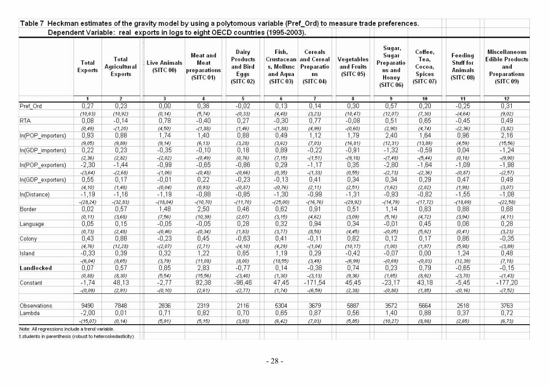
Tables 6 and 7 summarize the estimates obtained by using the procedure suggested by Heckman (1979). Looking first at the findings obtained when using separate dummies for the different preference schemes, the hypothesis of selection bias appears mostly supported by the evidence, as the lambda coefficient is always statistically significant, except for the total agricultural exports estimation. The results

32 This is the case when preferences influence not only the existing trade volume, but also when they open

new trade routes. Disregarding zero trade observations translates into ignoring new trade, and this could lead to underestimating the effect of preferences on developing countries’ exports (Helpmam, Melitz and Rubistein, 2006; Piermartini and The, 2005). In more rigorous terms, the potential sample selection bias is due to the fact that the process underlying the decision to export might be correlated with the gravity equation used to model the actual exports. If this correlation exists, disregarding the selection process yields biased estimates.

33 Since the two equations have the same specification, the non-linearity of lambda is the sole source of identification of the Heckman model. In fact, we find that exclusion restrictions are difficult to motivate either on a theoretical or an empirical ground. To give an example, in principle, a variable such as the common language might be thought as determinant of the decision to trade, which is not related to the amount actually traded. However, the same variable turns out to be often significant in the main equations we estimate. Thus, it could be excluded from the gravity equations for theoretical but not for statistical considerations. On the other hand, when, as a robustness check, we add the reporter fixed effects to the selection equation, results are substantially unaltered. It is worth noticing that these fixed effects are not significant in many equations. For the sake of conciseness, this evidence is not reported, but is available on request.

- 26 -

regarding the total exports flows confirm the positive sign and the significance of the ordinary GSP and the other preference dummies. Behind this aggregate effect, however, once again, there is a certain degree of unevenness across the groups of products. In fact, when considering agricultural exports at 2-digil level, the ordinary GSP dummy exerts a negative impact in many cases, while the other preference variable is negative only for the Feeding Stuff for Animals line. Finally, passing from LSDV to the Heckman estimation, most of the coefficients under scrutiny maintain their sign and significance. Yet, their magnitude generally increases passing from one method to the other.

When turning to the polytomous variable, the lambda coefficient is, again, always statistically significant, apart from the total agriculture estimation. Hence, in the latter case, the LSDV estimates are the more efficient. The coefficient of interest is positive and significant in the total exports case, as well as for many 2-digit groups of products. At the commodity level, an interesting result is that, when correcting for selection bias, the estimated impact of preferential treatment is always higher than when we only control for unobserved country heterogeneity. At the most aggregate level, the results are substantially the same as when applying the LSDV approach, both in term of sign and significance.

In order to summarize these results we draw two conclusions. Firstly, we show that aggregation matters: indeed, the positive effects obtained when analysing total exports hide a certain degree of unevenness across commodities. This specifically holds for the ordinary GSP. Secondly, we find that for any given level of data aggregation, the estimators we consider yield a slightly different impact of trade preferences. This impact appears to increase when accounting for zero-trade observations.

- 28 -

9 Conclusions This paper contributes to the empirical literature which uses gravity models to assess the impact of non reciprocal preferential trade policies (NRPTPs) granted by developed to developing countries.

After reviewing the related literature, we identify two key aspects that need further investigation. Firstly, we argue that the assessment of the impact of trade preferences should be carried out using disaggregated data rather than total exports, as discriminatory trade agreements apply at product level. Secondly, we advocate the use of estimators that control for unobserved heterogeneity, non-random selection bias and for the endogeneity of preferential treatment.

In order to support our claims, we analyse export flows towards eight OECD members (EU, USA, Japan, Norway, Switzerland, Australia, Canada and New Zealand) and employ three levels of data aggregation (total exports, total agricultural exports and 2-digit agricultural products). The coverage of trade preferences is very comprehensive, as the OECD countries we consider grant most of the NRPTPs currently active. The sensitivity of results to different estimation methods has been verified by using the OLS, a fixed effects model and Heckman estimators. The empirical results can be summarized as follows.

A first key evidence refers to the positive impact of trade preferences on total exports of beneficiaries, whatever the estimator. This finding is found in all the regressions we run using a polytomous variable to proxy the preferential treatments and is largely confirmed when we consider separate and mutually exclusive dummy variables for each preferential scheme (Ordinary GSP, GSP for LDCs and Other Preferences). The same applies for regressions used to explain total agricultural exports.

A second outcome concerns the effectiveness of trade preferences at 2-digit level. Limiting the discussion to the estimations obtained using Heckman’s method, it emerges that the effect of ordinary GSP, GSP for LDCs and Other preferences is not always positive and statistically significant. When this evidence is compared to that obtained at aggregated level it reveals how the aggregation influences the impact of trade preferences. We find that the NRPTPs granted by OECD members to developing countries are not always a story of success, as we obtain when using aggregated data: some sectors gain from the status of being preferred in terms of access into OECD markets, while others do not. This is not an unexpected outcome, which might be due to the fact that the margin of trade preferences widely varies across sectors.

A third result is that related to the heterogeneity of the impact of trade preferences across sectors and preferential schemes. For instance, the estimated impact of ordinary GSP is negative in many 2-digit groups and this evidence might depend on the high costs of complying with the relevant rules of origin that are required of exporters by OECD countries under the GSP scheme. Furthermore, the coefficient associated with the GSP for LDCs is positive in 6 out 10 sectors. This finding is consistent with the fact that the preferences granted by OECD countries to LDCs through the GSP are larger than those given under the ordinary GSP. Finally, the effect of trade preferences other than GSP is positive and highly significant in 8 out of 10 sectors, positive but non significant in the sector of dairy products and significantly negative only for the feeding stuff for animals industry. Again at 2-digit level, when using the ordered variable, we find that the effectiveness of NRPTPs is positive and significant in many groups of products.

- 30 -

Finally, the results allow us to verify the hypothesis according to which the impact of NRPTPs is underestimated when gravity models are estimated using overall exports. The paper does not provide robust evidence in this direction. For instance, in regressions based on the Heckman procedure, the hypothesis is validated in 11 out of 30 cases when using dummy variables and in 4 out of 10 cases when using the polytomous variable. Thus, the bias of aggregation differs sector by sector: with respect to gravity models which use data at 2-digit level, those that consider total exports either underestimate or overestimate the impact of NRPTPs granted by OECD to developing countries.

Although the NRPTPs increase, on average, the overall exports of beneficiary countries, we also show how estimations are heterogeneous across 2-digit sectors and data aggregations. Therefore, the paper should be considered only as a first step in a promising line of research. While we have mostly focused on evaluating the impact of NRPTPs using gravity equations and modelling trade preferences with the dummy variables approach, future work should refine the measures of preferential treatments. More broadly speaking, a natural next step is to conduct empirical analyses at very disaggregated level and to include in the gravity equation explicit measures of the trade preferences granted to the exports of developing countries. Conclusions that have been drawn about the role of NRPTPs are likely to be revised after reducing the measurement error of preferential treatments.

- 31 -

Appendix A: The exporting countries included in the sample Afghanistan, Albania, Algeria, Andorra, Angola, Antigua and Barbuda, Argentina, Armenia, Aruba, Australia, Austria, Azerbaijan, Bahamas, Bahrain, Bangladesh, Barbados, Belarus, Belize, Benin, Bermuda, Bhutan, Bolivia, Bosnia Herzegovina, Botswana, Brazil, Brunei Darussalam, Bulgaria, Burkina Faso, Burundi, Cambodia, Cameroon, Canada, Cape Verde, Cayman Islands, Central African Republic, Chad, Chile, China, China Hong Kong SAR, China Macao SAR, Colombia, Comoros, Congo, Costa Rica, Croatia, Cuba, Cyprus, Czech Republic, Democratic People's Republic of Korea, Democratic Republic of the Congo, Djibouti, Dominica, Dominican Republic, EU15, Ecuador, Egypt, El Salvador, Equatorial Guinea, Eritrea, Estonia, Ethiopia, FS Micronesia, Fiji, Finland, French Polynesia, Gabon, Gambia, Georgia, Ghana, Greenland, Grenada, Guatemala, Guinea, Guinea-Bissau, Guyana, Haiti, Honduras, Hungary, Iceland, India, Indonesia, Iran, Iraq, Israel, Ivory Coast, Jamaica, Japan, Jordan, Kazakhstan, Kenya, Kiribati, Kuwait, Kyrgyzstan, Lao People's Democratic Republic, Latvia, Lebanon, Lesotho, Liberia, Libya, Lithuania, Madagascar, Malawi, Malaysia, Maldives, Mali, Malta, Marshall Islands, Mauritania, Mauritius, Mayotte, Mexico, Mongolia, Morocco, Mozambique, Myanmar, Namibia, Nether. Antilles, New Caledonia, New Zealand, Nicaragua, Niger, Nigeria, Norway, Oman, Pakistan, Palau, Panama, Papua New Guinea, Paraguay, Peru, Philippines, Poland, Republic of Korea, Republic of Moldova, Romania, Russian Federation, Rwanda, Saint Kitts and Nevis, Saint Lucia, Saint Vincent and the Grenadines, Samoa, Sao Tome and Principe, Saudi Arabia, Senegal, Serbia and Montenegro, Seychelles, Sierra Leone, Singapore, Slovakia, Solomon Islands, Somalia, South Africa, Sri Lanka, Sudan, Suriname, Swaziland, Sweden, Switzerland, Syria, TFYR of Macedonia, Tajikistan, Thailand, Timor-Leste, Togo, Tonga, Trinidad and Tobago, Tunisia, Turkey, Turkmenistan, USA, Uganda, Ukraine, United Arab Emirates, United Republic of Tanzania, Uruguay, Uzbekistan, Vanuatu, Venezuela, Vietnam, Yemen, Zambia, Zimbabwe. Appendix B: Bilateral trade agreements covered USA-Israel (since 1985), USA-Jordan (since 2001), NAFTA (USA-Mexico and Canada, since 1994), Australia-New Zealand (since 2003), Australia-Singapore (since 2003), New Zealand-Singapore (since 2001), Australia-Papua New Guinea, Japan-Singapore (since 2002), Canada-Chile (since 1997), Canada-Costa-Rica (2002), Canada-Israel (since 1997), the RTAs of EU15 with Iceland, Norway/EFTA, Switzerland/EFTA, Algeria, Syria, Andorra (since 1991), Bulgaria and Romania (1993), Turkey (1996), Tunisia (1998), Israel (2000), Mexico (2000), Morocco (2000), South Africa (2000), Republic of Macedonia (2001), Croatia (2002) Jordan (2002), Chile and Lebanon (2003). Finally, we consider the preferences granted by EFTA members (Norway and Switzerland) to Turkey (1992), Bulgaria (1994), Israel and Romania (1993), Morocco (2000), Republic of Macedonia (2001), Mexico (2001), Croatia (2002), Jordan (2002) and Singapore (2003). We do not consider the RTA signed after 2003 [such as EU and Egypt (2004), USA and Chile (2004), USA and Singapore (since 2004), EFTA and Chile (2004)].

- 32 -

References Aitken N.D. (1973), The effect of the EEC and EFTA on European Trade: a temporal

cross-section analysis, American Economic Review, 63, 881-892. Amurgo-Pacheco A. (2006), Preferential Trade Liberalization and the Range of

Exported Products: The Case of the Euro-Mediterranean FTA. HEI Working Paper No: 18/2006, Graduate Institute of International Studies, Geneva.

Anderson J.E., Wincoop E. (2004), Trade costs, Journal of Economic Literature, 42, 3, 691-751.

Bureau J.C., Chakir R., Gallezot J. (2006), The Utilisation of EU and US Trade Preferences for Developing Countries in the Agri-Food Sector, TRADEAG Working Paper No. 19/2006 (downloadable from http://tradeag.vitamib.com).

Baltagi B.H., Egger P., Pfaffermayr M. (2003), A generalized design for bilateral trade flow models, Economic Letters, 80, 391-397.

Burfisher M., Pick D., Pompelli, G., Zahniser S. (2001), North American trade in an Era of Multiple Trade Agreements: A Gravity Analysis. Paper presented at the annual meeting, American Agricultural Economics Association and Canadian Agricultural Economic Society, Chicago, August 5-8.

Cardamone P. (2007), A survey of the Assessments of the Effectiveness of Preferential Trade Agreements using Gravity Models, TRADEAG Working Paper, (downloadable from http://tradeag.vitamib.com).

Carrère C. (2006), Revisiting the Effects of Regional Trade Agreements on Trade Flows with Proper Specification of the Gravity Model, European Economic Review, forthcoming.

Chaney T. (2005), Distorted Gravity: Heterogeneous Firms, Market Structure and the Geography of International Trade, Job market paper, MIT.

Cheng I., Wall H. J. (2002), Controlling for Heterogeneity in Gravity Models of Trade, Working Paper 1000-010C , Federal Reserve Bank of St. Louis.

Coe D.T., Subramanian A., Tamirisa N.T. (2002), The Missing Globalization Puzzle. IMF Working Paper 02/171.

Davidson R., MacKinnon J. (1993), Estimation and Inference in Econometrics, New York: Oxford University Press.

Egger P. (2002), An Econometric View on the Estimation of Gravity Models and the Calculation of Trade Potentials, The World Economy, 25, 297-312.

Egger P., Pfaffermayr M. (2003), The proper panel econometric specification of the gravity equation: A three-way model with bilateral interaction effects, Empirical Economics, 28, 571-580.

Emlinger C., Chevasuss Lozza E., Jacquet F. (2006). EU Market Access for Mediterranean fruit and vegetables: A gravity mode assessment. Paper presented at the ETSG 2006 – 8th Annual Conference, 7-9 September 2006, WiW Universität, Wien.

European Commission (1998), Development: the Lomè trade regime, Bruxelles. Felbermayr G.J., Kohler W. (2004), Exploring the Intensive and Extensive Margins of

World Trade, CESIFO Working Paper N. 1276, Francois J., Hoekman B., Manchin M. (2005), Preference Erosion and Multilateral

Trade Liberalization, Discussion Paper 2005-073/2, Tinbergen Institute. Frankel J., Stein E., Wei S. (1995), Trading blocs and the Americas: the natural, the

unnatural, and the supernatural, Journal of Development Economics, 47, 61-95.

- 33 -

Gaulier G., Zignago S. (2005), The Role of Proximity and Similarity in trade of Goods, mimeo, CEPII, Paris.

Garcia-Alvarez-Coque J.M, Marti Selva M.L. (2006), A Gravity Approach to Assess the Effects of Association Agreements on Euro-Mediterranean Trade of Fruits and Vegetables, TRADEAG Working Paper No. 12/2006 (downloadable from http://tradeag.vitamib.com).

Gaulier G., Jean S., Ünal-Kesenci D. (2004). Regionalism and the Regionalisation of International Trade. CEPII Working Paper No 2004-16.

Gleditsch K. S. (2002), Expanded Trade and GDP Data. Journal of Conflict Resolution 46(5), 712-724.

Goldstein J., Rivers D., Tomz M. (2003), How Does the Trade Regime Affect International Trade?, Paper prepared for the annual meetings of the American Political Science Association, Philadelphia, PA, August 28-31, 2003.

Halvrsen R., Palmquist R. (1980), The interpretation of dummy variable in semi-logarithmic regressions, American Economic Review, 70: 474-75.

Hansen B.E. (2000), Sample Splitting and Threshold Estimation, Econometrica, 68, 575-603.

Hausman J., Taylor W. (1981), Panel Data and Unobservable Individual Effects, Econometrica, 49, 1377-1398.

Harris M. N., Màtyàs L., (1988), The Econometrics of Gravity Models, Working Paper 5/98, Melbourne Institute.

Helpman E., Melitz M., Rubinstein Y. (2006), Trading Partners and Trading Volumes, Discussion paper, Harvard University.

Heckman J,J. (1979), Sample Selection Bias as a Specification Error, Econometrica, 47, 1, 153-162.

Jayasinghe S., Sarker R. (2004), Effects of RTA on Trade in Agri-food Products: Evidence from Gravity Modelling Using Disaggregated Data, 04-WP 374, CARD, Iowa State University.

Lederman D., Özden Ç. (2004), U.S. Trade Preferences: All Are Not Created Equal. Unpublished, World Bank, Washington DC.

Manchin M. (2004), Preference Utilisation and Tariff Reduction in EU Imports from ACP Countries, Discussion Paper 2004-132/2, Tinbergen Institute.

Mátyás L. (1997), Proper econometric specification of the gravity model, The World Economy, 20, 363-368.

Mold A. (2004), Trade Preference and Africa – The State of Play and the Issue at State, mimeo, The African Trade Policy Centre of the Economic Commission for Africa, United Nation, Economic Commission for Africa.

Nielsen C. P. (2003), Regional and Preferential Trade Agreements: a Literature Review and Identification of Future Steps, Report n. 155, Fodevareokonomisk Institut, Copenhagen.

Nilsson L. (2002), Trading relations: is the roadmap from Lomé to Cotonou correct?, Applied Economics, 34, 439-452.

Nilsson L. (2005), Comparative effects of EU and US trade policies on developing country exports, mimeo, European Commission, Trade DG.

Nouve K., Staatz J. (2003), Has AGOA Increased Agricultural Exports from Sub-Saharan Africa to the United States?, paper presented at the International Conference Agricultural policy reform and the WTO: where are we heading), Capri (Italy), June 23-26.

- 34 -

Oguledo V.I., MacPhee C.R. (1994), Gravity Models: a reformulation and an application to discriminatory trade arrangements, Applied Economics, 26, 107-120.

Özden C., Reinhardt (2004), First do not harm. The Effect of Trade Preferences on Developing Country Exports, mimeo, World Bank. Washington DC.

Özden C., Reinhardt E. (2005), The perversity of preferences: GSP and developing country trade policies, 1976–2000, Journal of Development Economics , 78, pp. 1–21.

Persson M., Wilhelmsson F. (2005), Revisiting the Effect of EU Trade Preferences, mimeo, Lund University.

Piermartini R., The R. (2005), Demystifying Modelling Methods for Trade Policy, World Trade Organization, Discussion Paper 10, Geneva, Switzerland.

Pöyhonen P. (1963), A Tentative Model for the Volume of Trade between Countries, Weltwirtschaftliches Archiv, 90(1), 93-99.

Pusterla F. (2007), Regional Integration Agreements: impact, Geography and Efficiency. IDB-SOE Working Paper, January 2007.

Rose A. (2003), Which international institutions promote international trade? CEPR Discussion Paper 3764 (Review of International Economics, forthcoming).

Rose A. (2004), Do We Really Know that the WTO increases Trade?, American Economic Review, vol. 94(1), 98-114.

Rose A. (2005), Does the WTO Make Trade More Stable? Open Economies Review, 16 (1), 7-22.

Serlenga L., Shin Y. (2004), Gravity Models of the Intra-EU Trade: Application of the Hausman-Taylor Estimation in Heterogeneous Panels with Common Time-specific Factors, ESE Discussion Paper n. 105.

Silva Santos J.M.C., Tenreyro S. (2003), Gravity-Defying Trade, mimeo, Federal Reserve Bank of Boston, Boston.

Subramanian A., Wei S.J. (2005), The WTO promotes trade, strongly but unevenly. CEPR Discussion Paper No 5122.

Tinbergen J. (1962), Shaping the World Economy: Suggestions for and International Economic Policy, New York: the Twentieth Century Fund.

Verdeja L. (2006), EU’s Preferential Trade Agreements With Developing Countries Revisited, Unpublished, University of Nottingham, School of Economics.

Wooldridge J. M. (2002), Econometric Analysis of Cross Section and Panel Data, Cambridge, MA: MIT Press.

Wooldridge J. M. (2003), Introductory Econometrics. A Modern Approach. 2E, Thomson South Western.