Analysis and Approximation of a Fractional Differential Equation Marcus Webb Supervisors: Prof. Endre S¨ uli Dr David Kay Part C Mathematics Dissertation University of Oxford Hilary Term, 2012
Transcript
Analysis and Approximation ofa Fractional Differential
Equation
Marcus Webb
Supervisors:
Prof. Endre Suli
Dr David Kay
Part C Mathematics Dissertation
University of OxfordHilary Term, 2012
Abstract
A differential equation is fractional if it involves an operator that can be considered to
be between a (k − 1)th and kth order differential operator, for some positive integer k,
and it is said to be of fractional-order if this operator is the highest order operator in the
equation. The diffusion equation is of order 2, because its highest order operator is the
Laplacian, a 2nd order differential operator, but we can consider an analogous equation
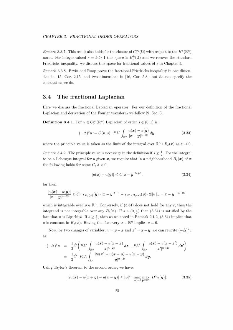
of order 2s, where s ∈ (0, 1), involving the so-called fractional Laplacian operator. Such
fractional-order equations appear in a surprising number of real world models. For
example, a diffusion model used for cardiac tissue is what is known as anomalous, or
non-Fickian, because the diffusion does not satisfy Fick’s law of diffusion and is not
modelled accurately by the diffusion equation, but actually by a differential equation
of fractional order. The diffusion is also anisotropic (directionally dependent) because
diffusion along fibers happens at a different rate to that across fibers in the tissue; the
mathematical models of are harder to work with. This thesis covers some analysis for
the study of fractional-order advection-diffusion equations relevant to this anisotropic
cardiac tissue model.
The study of fractional-order equations is difficult: Firstly, fractional-order opera-
tors are nonlocal, i.e. the value of a fractional derivative of a function at a point in
the domain depends on values of the function throughout the domain; and secondly,
boundary conditions (traces) do not make sense in fractional Sobolev spaces of order
s ≤ 1/2, so constraints must be defined on a region of non-zero volume. We review
and derive some relevant results on fractional Sobolev spaces, fractional-order operators
and the nonlocal calculus developed by Du, Gunzburger, Lehoucq, Zhou (2011). We
prove well-posedness of a general class of fractional-order elliptic problems and develop
Galerkin approximations, focusing on the derivation of a-priori error bounds.
Preface
This thesis is a fourth year mathematics dissertation worth a whole unit towards the
degree of Master of Mathematics and Computer Science.
The target audience is a fourth year undergraduate at Oxford who has taken the
C5.1a Methods of Functional Analysis for PDEs and C12.2b Finite Element Methods
for PDEs courses. In particular, we assume that the reader is familiar with the following
concepts:
• For k ∈ N, 1 ≤ p ≤ ∞, and open subsets Ω of Rn, basic properties of:
– The Lebesgue spaces Lp(Ω)
– The Sobolev spaces W k,p(Ω), Hk(Ω)
– Continuous function spaces C(Ω), Ck(Ω), C∞(Ω)
– The space of infinitely differentiable functions with compact support C∞0 (Ω)
• The finite element method for second-order elliptic PDEs
• A priori and a posteriori error analysis of these methods
I would like to thank my supervisors David and Endre for their stimulating discus-
sions in our regular meetings, and for their support and encouragement throughout the
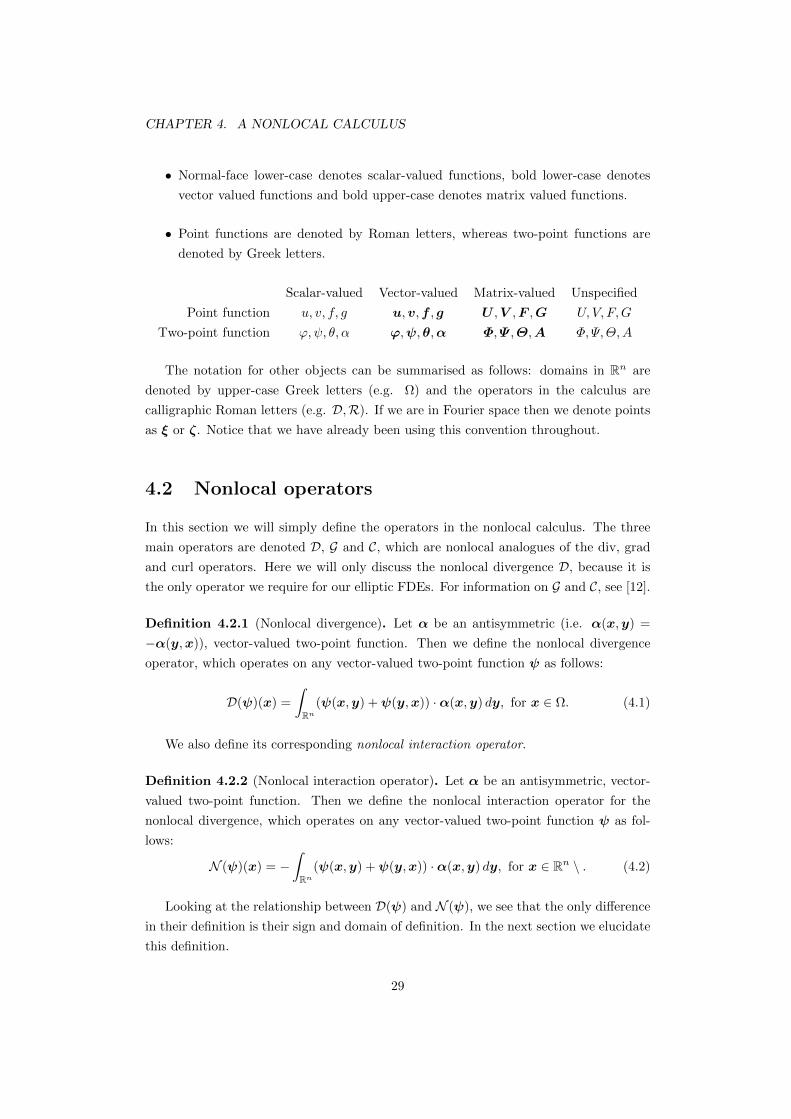
Point function u, v, f, g u,v,f , g U ,V ,F ,G U, V, F,G
Two-point function ϕ,ψ, θ, α ϕ,ψ,θ,α Φ,Ψ ,Θ,A Φ, Ψ,Θ,A
The notation for other objects can be summarised as follows: domains in Rn are
denoted by upper-case Greek letters (e.g. Ω) and the operators in the calculus are
calligraphic Roman letters (e.g. D,R). If we are in Fourier space then we denote points
as ξ or ζ. Notice that we have already been using this convention throughout.
4.2 Nonlocal operators
In this section we will simply define the operators in the nonlocal calculus. The three
main operators are denoted D, G and C, which are nonlocal analogues of the div, grad
and curl operators. Here we will only discuss the nonlocal divergence D, because it is
the only operator we require for our elliptic FDEs. For information on G and C, see [12].
Definition 4.2.1 (Nonlocal divergence). Let α be an antisymmetric (i.e. α(x,y) =
−α(y,x)), vector-valued two-point function. Then we define the nonlocal divergence
operator, which operates on any vector-valued two-point function ψ as follows:
D(ψ)(x) =
∫Rn
(ψ(x,y) +ψ(y,x)) ·α(x,y) dy, for x ∈ Ω. (4.1)
We also define its corresponding nonlocal interaction operator.
Definition 4.2.2 (Nonlocal interaction operator). Let α be an antisymmetric, vector-
valued two-point function. Then we define the nonlocal interaction operator for the
nonlocal divergence, which operates on any vector-valued two-point function ψ as fol-
lows:
N (ψ)(x) = −∫Rn
(ψ(x,y) +ψ(y,x)) ·α(x,y) dy, for x ∈ Rn \ . (4.2)
Looking at the relationship between D(ψ) and N (ψ), we see that the only difference
in their definition is their sign and domain of definition. In the next section we elucidate
this definition.
29
4.3. PROPERTIES OF THE NONLOCAL CALCULUS
4.3 Properties of the nonlocal calculus
The Gauss-Green Divergence Theorem for a vector-valued function f ∈ H1(Ω) is as
follows [17, p. 711]: ∫Ω
∇ · f dx =
∫∂Ω
m · f dS, (4.3)
where m is the outward unit normal vector for the C1 domain Ω. The following lemma
shows how the nonlocal operators are defined specifically to satisfy an analogous theorem.
Lemma 4.3.1 (Fundamental lemma of the nonlocal calculus). Any two-point function
Ψ ∈ L1(Rn × Rn), which is antisymmetric, has the following property:∫Rn
∫Rn
Ψ(x,y) dy dx = 0. (4.4)
Proof. First we use antisymmetry, then using Fubini’s theorem [23, p. 25] we can the
order of integration:∫Rn
∫Rn
Ψ(x,y) dy dx = −∫Rn
∫Rn
Ψ(y,x) dy dx
= −∫Rn
∫Rn
Ψ(y,x) dx dy
= −∫Rn
∫Rn
Ψ(x,y) dy dx. (4.5)
The last step is a relabelling of dummy variables.
Corollary 4.3.2 (Nonlocal divergence theorem). For D and N defined as in section
4.2 and any vector-valued two-point function ψ we have:∫Ω
D(ψ) dx =
∫Rn\Ω
N (ψ) dx. (4.6)
Proof. Note that α is antisymmetric and ψ(x,y) +ψ(y,x) is symmetric, so ψ(x,y) +
ψ(y,x)) ·α(x,y) is antisymmetric. Hence,∫Ω
D(ψ) dx−∫Rn\Ω
N (ψ) dx =
∫Rn
∫Rn
(ψ(x,y) +ψ(y,x)) ·α(x,y) dy dx = 0.
Rearranging gives us the desired equation.
For the classical calculus, we also have the integration by parts formula. For scalar-
valued u ∈ H1(Ω) and vector-valued v ∈ H1(Ω), this is the following:∫Ω
u(∇ · v) dx+
∫Ω
(−∇u) · v dx =
∫∂Ω
u(m · v) dS, (4.7)
where m is the outward unit normal vector for the C1 domain Ω. This equation can be
interpreted as saying that the negative gradient −∇ is a formal adjoint to the divergence
operator ∇·. Let us define the adjoint of a nonlocal operator in this way, and find it
explicitly, to have a nonlocal integration by parts formula.
30
CHAPTER 4. A NONLOCAL CALCULUS
Definition 4.3.3 (Nonlocal adjoint). For a nonlocal operator E with associated inter-
action operator X , its nonlocal adjoint is an operator E∗ such that, for functions Φ and
P : ∫Ω
PE(Φ) dx−∫Rn
∫RnE∗(P )Φdy dx =
∫Rn\Ω
PX (Φ) dx. (4.8)
Here Φ and P can be scalar- or vector-valued, depending on E .
Proposition 4.3.4 (Adjoint for nonlocal divergence). For D and N as defined in Sec-
tion 4.2, the adjoint for the nonlocal divergence is the operator D∗ such that for all
scalar-valued functions u:
D∗(u)(x,y) = (u(x)− u(y))α(x,y) ∀x,y ∈ Rn. (4.9)
Proof. Let ψ be a vector-valued two-point function. Then, using the fundamental
Lemma 4.3.1 to get the penultimate line,∫Ω
uD(ψ) dx−∫Rn\Ω
uN (ψ) dx
=
∫Rn
∫Rnu(x)(ψ(x,y) +ψ(y,x)) ·α(x,y) dy dx
=
∫Rn
∫Rn
(u(x)ψ(x,y)− u(y))ψ(x,y)) ·α(x,y) dy dx
+
∫Rn
∫Rn
(u(x)ψ(y,x) + u(y)ψ(x,y)) ·α(x,y) dy dx
=
∫Rn
∫Rn
(u(x)− u(y))α(x,y)ψ(x,y) dy dx
=
∫Rn
∫RnD∗(u)ψ(x,y) dy dx.
This completes the proof.
Corollary 4.3.5. [Nonlocal integration by parts] Let u be a scalar-valued one-point
function and let ψ be a vector-valued two-point function; then:∫Ω
uD(ψ) dx−∫Rn
∫RnD∗(u) ·ψ dy dx =
∫Rn\Ω
uN (ψ) dx. (4.10)
Proof. This is a restatement of Proposition 4.3.4.
From the integration by parts formula for classical derivatives, we can derive Green’s
first identity by setting v = A∇w for a matrix-valued function A ∈ C1(Ω) and a scalar-
valued function w ∈ H2(Ω):∫Ω
u(∇ ·A∇w) dx+
∫Ω
(−∇u) ·A∇w dx =
∫∂Ω
um ·A∇w dS, (4.11)
For the nonlocal calculus we can do the same by setting φ = ΘD∗(v) in the in-
tegration by parts formula, where v is a scalar-valued two-point function and Θ is a
matrix-valued two-point function (because D∗(v) is a two-point function).
31
4.4. INCLUSION OF THE CLASSICAL VECTOR CALCULUS
Theorem 4.3.6 (Nonlocal Green’s identity). Let D and N be the nonlocal divergence
and interaction operators as defined in Section 4.2, u and v scalar-valued one-point
functions and Θ a matrix-valued two-point functions. Then:∫Ω
uD(ΘD∗(v)) dx−∫Rn
∫RnD∗(u) ·ΘD∗(v) dy dx =
∫Rn\Ω
uN (ΘD∗(v)) dx (4.12)
Proof. Let ψ = ΘD∗(v) in Corollary 4.3.5.
Remark 4.3.7. Note that we use the entire complement of Ω (which is Rn \ Ω) for the
domain of the interaction function N (ψ). This means that in general there is no upper
limit on the distance of a nonlocal interaction. This need not be the case; for example if
α has support in the strip (x,y) : |x− y| < ε then nonlocal interactions are confined
within balls of radius ε. Then the interaction function N (ψ) has support in an ε-thin
strip surrounding Ω.
Given the theorems discussed in this section, we see a direct correspondence between
the operators of the nonlocal calculus: D, D∗ and N ; and those of the classical calcu-
lus: div, grad and the normal flux operator. In the next section we discuss how this
correspondence can be taken further.
4.4 Inclusion of the classical vector calculus
Du et al. showed that this nonlocal calculus generalises the classical vector calculus in
a distributional sense [12]. In other words, there is a choice of α (which is a distribu-
tion rather than a function) such that the nonlocal operators are effectively the classical
differential operators. By effectively we mean that this correspondence will not be per-
fect, because nonlocal operators involve two-point functions whereas classical differential
operators only involve one-point functions.
We try to be brief here to avoid losing focus; we include this discussion because we
take a slightly different approach to the one given in the original paper. Define the
antisymmetric α kernel to be the distribution:
α(x,y) = −∇yδ(y − x). (4.13)
This is “physicist’s notation” [34, p. 26] for the distribution Tα(x,·) such that for all
w ∈ C∞0 (Rn),
Tα(x,·)(w) = ∇ ·w(x) (4.14)
Again in physicist’s notation:
Tα(x,·)(w) =
∫Rnw(y) ·α(x,y) dy
=
∫Rnw(y) · (−∇y)δ(y − x) dy
32
CHAPTER 4. A NONLOCAL CALCULUS
=
∫Rn
(∇ ·w)δ(y − x) dy
= ∇ ·w(x).
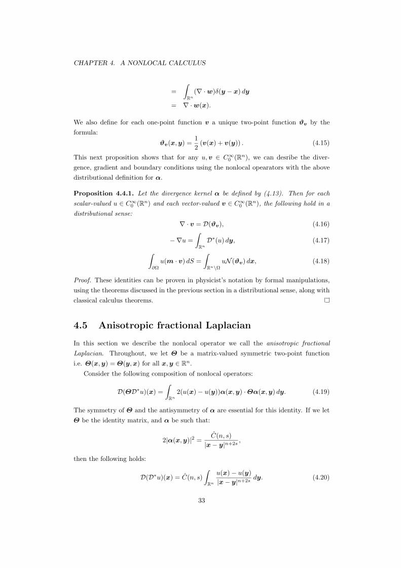
We also define for each one-point function v a unique two-point function ϑv by the
formula:
ϑv(x,y) =1
2(v(x) + v(y)) . (4.15)
This next proposition shows that for any u,v ∈ C∞0 (Rn), we can desribe the diver-
gence, gradient and boundary conditions using the nonlocal opearators with the above
distributional definition for α.
Proposition 4.4.1. Let the divergence kernel α be defined by (4.13). Then for each
scalar-valued u ∈ C∞0 (Rn) and each vector-valued v ∈ C∞0 (Rn), the following hold in a
distributional sense:
∇ · v = D(ϑv), (4.16)
−∇u =
∫RnD∗(u) dy, (4.17)∫
∂Ω
u(m · v) dS =
∫Rn\Ω
uN (ϑv) dx, (4.18)
Proof. These identities can be proven in physicist’s notation by formal manipulations,
using the theorems discussed in the previous section in a distributional sense, along with
classical calculus theorems.
4.5 Anisotropic fractional Laplacian
In this section we describe the nonlocal operator we call the anisotropic fractional
Laplacian. Throughout, we let Θ be a matrix-valued symmetric two-point function
i.e. Θ(x,y) = Θ(y,x) for all x,y ∈ Rn.
Consider the following composition of nonlocal operators:
D(ΘD∗u)(x) =
∫Rn
2(u(x)− u(y))α(x,y) ·Θα(x,y) dy. (4.19)
The symmetry of Θ and the antisymmetry of α are essential for this identity. If we let
Θ be the identity matrix, and α be such that:
2|α(x,y)|2 =C(n, s)
|x− y|n+2s,
then the following holds:
D(D∗u)(x) = C(n, s)
∫Rn
u(x)− u(y)
|x− y|n+2sdy. (4.20)
33
4.5. ANISOTROPIC FRACTIONAL LAPLACIAN
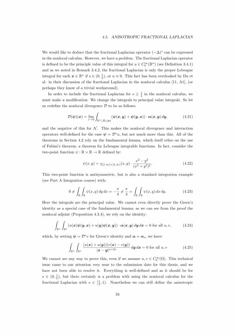
We would like to deduce that the fractional Laplacian operator (−∆)s can be expressed
in the nonlocal calculus. However, we have a problem. The fractional Laplacian operator
is defined to be the principle value of this integral for u ∈ C∞0 (Rn) (see Definition 3.4.1)
and as we noted in Remark 3.4.2, the fractional Laplacian is only the proper Lebesgue
integral for each x ∈ Rn if s ∈ (0, 12 ), or u ≡ 0. This fact has been overlooked by Du et
al. in their discussion of the fractional Laplacian in the nonlocal calculus [11, A1], (or
perhaps they know of a trivial workaround).
In order to include the fractional Laplacian for s ≥ 12 in the nonlocal calculus, we
must make a modification: We change the integrals to principal value integrals. So let
us redefine the nonlocal divergence D to be as follows:
D(ψ)(x) = limε→0
∫Rn\Bε(x)
(ψ(x,y) +ψ(y,x)) ·α(x,y) dy, (4.21)
and the negative of this for N . This makes the nonlocal divergence and interaction
operators well-defined for the case ψ = D∗u, but not much more than this. All of the
theorems in Section 4.2 rely on the fundamental lemma, which itself relies on the use
of Fubini’s theorem, a theorem for Lebesgue integrable functions. In fact, consider the
two-point function ψ : R× R→ R defined by:
ψ(x, y) = χ[1,∞)×[1,∞)(x, y) · x2 − y2
(x2 + y2)2. (4.22)
This two-point function is antisymmetric, but is also a standard integration example
(see Part A Integration course) with:
0 6=∫R
∫Rψ(x, y) dy dx = −π
46= π
4=
∫R
∫Rψ(x, y) dx dy. (4.23)
Here the integrals are the principal value. We cannot even directly prove the Green’s
identity as a special case of the fundamental lemma; as we can see from the proof the
nonlocal adjoint (Proposition 4.3.4), we rely on the identity:∫Rn
∫Rn
(u(x)ψ(y,x) + u(y)ψ(x,y)) ·α(x,y) dy dx = 0 for all u, v, (4.24)
which, by setting ψ = D∗v for Green’s identity and α = αs, we have:∫Rn
∫Rn
(u(x) + u(y))(v(x)− v(y))
|x− y|n+2sdy dx = 0 for all u, v (4.25)
We cannot see any way to prove this, even if we assume u, v ∈ C∞0 (Ω). This technical
issue came to our attention very near to the submission date for this thesis, and we
have not been able to resolve it. Everything is well-defined and as it should be for
s ∈ (0, 12 ), but there certainly is a problem with using the nonlocal calculus for the
fractional Laplacian with s ∈ [ 12 , 1). Nonetheless we can still define the anisotropic
34
CHAPTER 4. A NONLOCAL CALCULUS
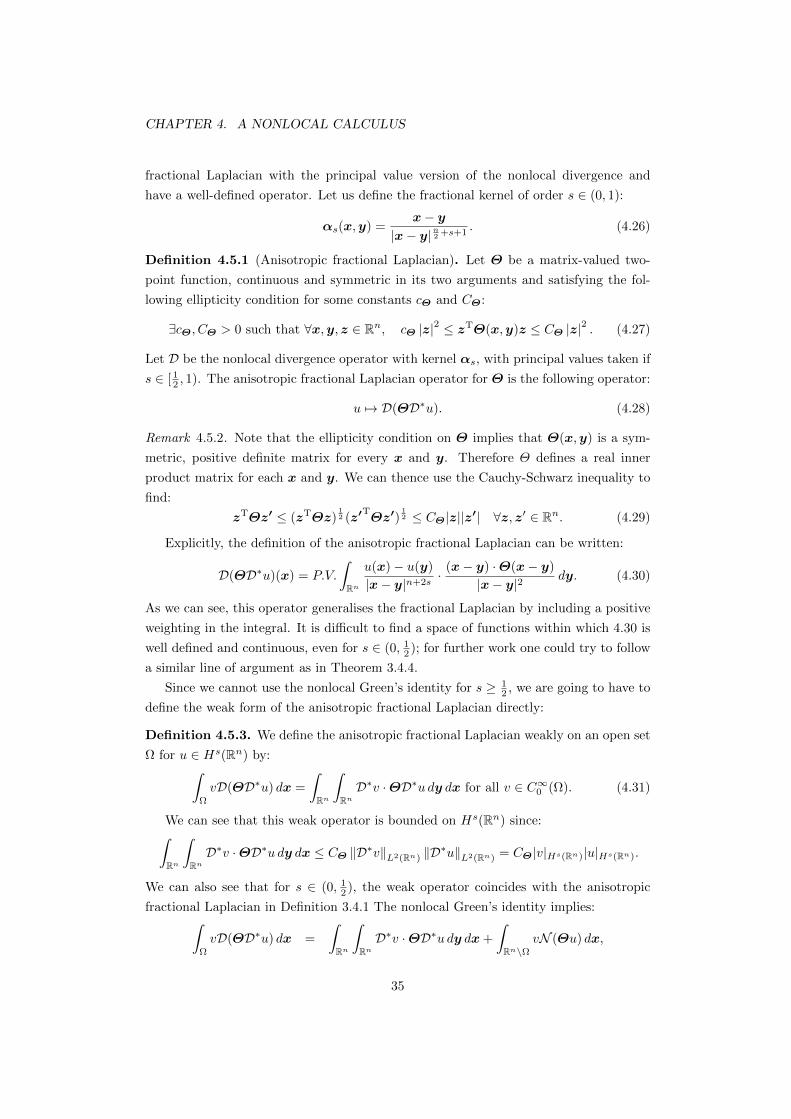
fractional Laplacian with the principal value version of the nonlocal divergence and
have a well-defined operator. Let us define the fractional kernel of order s ∈ (0, 1):
αs(x,y) =x− y
|x− y|n2 +s+1. (4.26)
Definition 4.5.1 (Anisotropic fractional Laplacian). Let Θ be a matrix-valued two-
point function, continuous and symmetric in its two arguments and satisfying the fol-
lowing ellipticity condition for some constants cΘ and CΘ:
∃cΘ, CΘ > 0 such that ∀x,y, z ∈ Rn, cΘ |z|2 ≤ zTΘ(x,y)z ≤ CΘ |z|2 . (4.27)
Let D be the nonlocal divergence operator with kernel αs, with principal values taken if
s ∈ [ 12 , 1). The anisotropic fractional Laplacian operator for Θ is the following operator:
u 7→ D(ΘD∗u). (4.28)
Remark 4.5.2. Note that the ellipticity condition on Θ implies that Θ(x,y) is a sym-
metric, positive definite matrix for every x and y. Therefore Θ defines a real inner
product matrix for each x and y. We can thence use the Cauchy-Schwarz inequality to
find:
zTΘz′ ≤ (zTΘz)12 (z′
TΘz′)
12 ≤ CΘ|z||z′| ∀z, z′ ∈ Rn. (4.29)
Explicitly, the definition of the anisotropic fractional Laplacian can be written:
D(ΘD∗u)(x) = P.V.
∫Rn
u(x)− u(y)
|x− y|n+2s· (x− y) ·Θ(x− y)
|x− y|2dy. (4.30)
As we can see, this operator generalises the fractional Laplacian by including a positive
weighting in the integral. It is difficult to find a space of functions within which 4.30 is
well defined and continuous, even for s ∈ (0, 12 ); for further work one could try to follow
a similar line of argument as in Theorem 3.4.4.
Since we cannot use the nonlocal Green’s identity for s ≥ 12 , we are going to have to
define the weak form of the anisotropic fractional Laplacian directly:
Definition 4.5.3. We define the anisotropic fractional Laplacian weakly on an open set
Ω for u ∈ Hs(Rn) by:∫Ω
vD(ΘD∗u) dx =
∫Rn
∫RnD∗v ·ΘD∗u dy dx for all v ∈ C∞0 (Ω). (4.31)
We can see that this weak operator is bounded on Hs(Rn) since:∫Rn
∫RnD∗v ·ΘD∗u dy dx ≤ CΘ ‖D∗v‖L2(Rn) ‖D
∗u‖L2(Rn) = CΘ|v|Hs(Rn)|u|Hs(Rn).
We can also see that for s ∈ (0, 12 ), the weak operator coincides with the anisotropic
fractional Laplacian in Definition 3.4.1 The nonlocal Green’s identity implies:∫Ω
vD(ΘD∗u) dx =
∫Rn
∫RnD∗v ·ΘD∗u dy dx+
∫Rn\Ω
vN (Θu) dx,
35
4.5. ANISOTROPIC FRACTIONAL LAPLACIAN
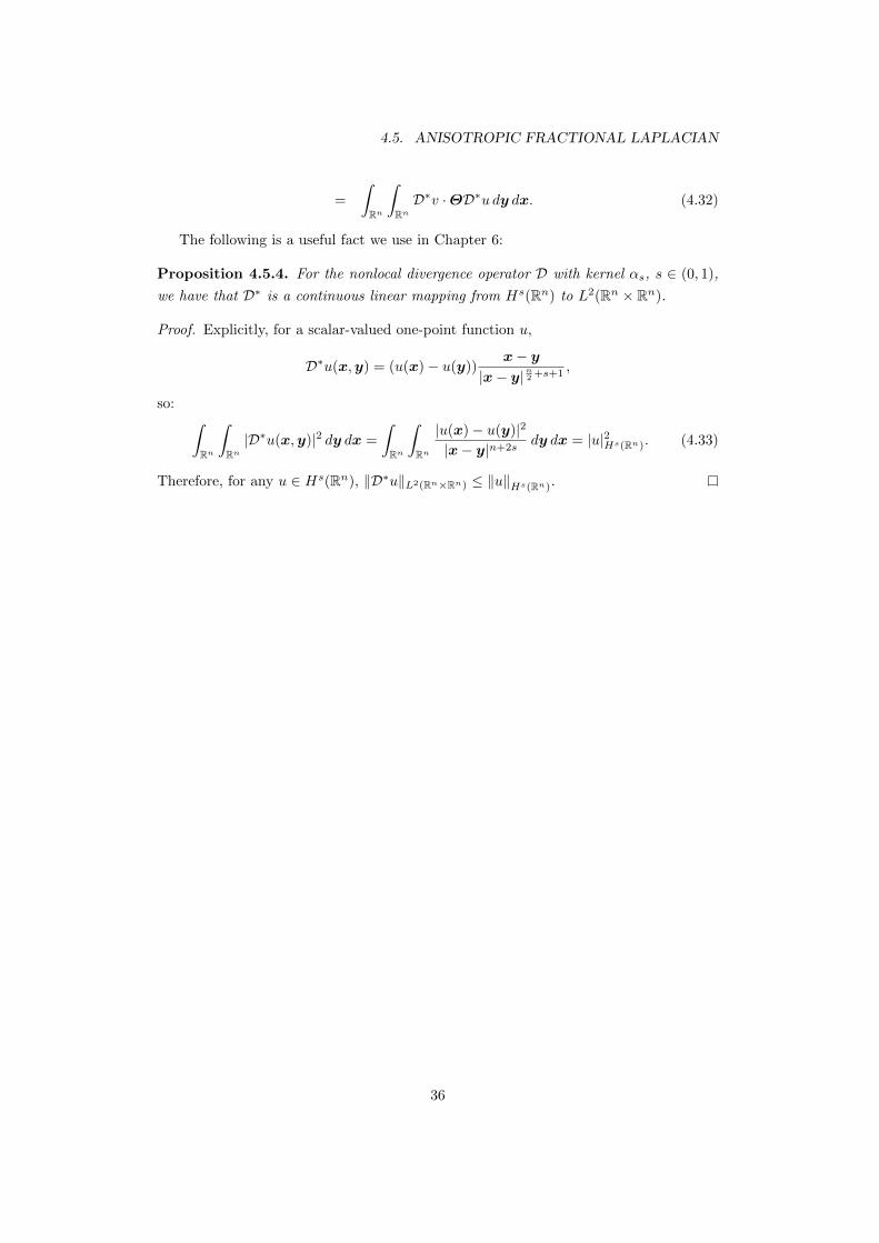
=
∫Rn
∫RnD∗v ·ΘD∗u dy dx. (4.32)
The following is a useful fact we use in Chapter 6:
Proposition 4.5.4. For the nonlocal divergence operator D with kernel αs, s ∈ (0, 1),
we have that D∗ is a continuous linear mapping from Hs(Rn) to L2(Rn × Rn).
Proof. Explicitly, for a scalar-valued one-point function u,
D∗u(x,y) = (u(x)− u(y))x− y
|x− y|n2 +s+1,
so: ∫Rn
∫Rn|D∗u(x,y)|2 dy dx =
∫Rn
∫Rn
|u(x)− u(y)|2
|x− y|n+2sdy dx = |u|2Hs(Rn). (4.33)
Therefore, for any u ∈ Hs(Rn), ‖D∗u‖L2(Rn×Rn) ≤ ‖u‖Hs(Rn).
36
Chapter 5
Volume-Constrained Problems
In this chapter we discuss the general form of some volume-constrained problems, and
reduce proving existence and uniqueness of solution to the non-homogeneous Dirichlet
volume-constrained problem to that of an homogeneous one.
5.1 Boundary value problems
This section will be slightly vague, as we use it just to motivate our treatment of the
volume-constrained problems. Dirichlet boundary-value problems on a bounded domain
Ω ⊂ Rn take the form of finding u in a function space V such that:
Lu = f in Ω,
u = g on ∂Ω.(5.1)
Here f and g are some prescribed functions defined on Ω and ∂Ω respectively, and Lis a differential operator. One way to start the analysis of such problems is to prove
that there exists a function g ∈ V defined on Ω such that g∂Ω = g. This follows from
surjectivity of a trace operator from V onto a space containing g (see Theorem 2.5.2).
Then we can rewrite the problem as follows:
Lu0 = f0 in Ω,
u0 = 0 on ∂Ω,(5.2)
where u0 = u− g and f0 = f −Lg [17, p. 315]. If we can prove existence and uniqueness
of a weak solution for this problem, then we have existence of a weak solution to problem
(5.1), which is u = u0 + g. By linearity of L, we also have uniqueness so long as 0 is
the unique solution to (5.1) with f ≡ 0 and g ≡ 0 (which follows from coercivity of the
bilinear form for the weak formulation).
37
5.2. VOLUME-CONSTRAINED PROBLEMS
For the particular case of V = H1(Ω), where Ω is a bounded Lipschitz domain, the
weak solutions to the homogeneous problem lie in the space:
H10 (Ω) :=
u ∈ H1(Ω) : Tu ≡ 0
. (5.3)
This is the space of zero-trace functions, where T is the trace operator on H1(Ω). One
can prove that for the case where Ω is a Lipschitz domain, this space is equal to the
closure of C∞0 (Ω) with respect to the H1(Ω) norm, which is denoted H10 (Ω) [17, p. 273].
Problems can then be tackled for C∞0 (Ω) functions before generalised to the whole of
the solution space by density.
We would like to do something similar for volume constrained problems: reduce the
problem to the homogeneous case and show that the homogeneous solution space has
dense subspace C∞0 (Ω).
5.2 Volume-constrained problems
Let Ω be a bounded open Lipschitz domain and let Ω be an open set containing the
closure of Ω. We denote Ωc = Ω\Ω ⊆ Rn\Ω. Let L be a differential operator of order 2s
where s ∈ (0, 1), f ∈ L2(Ω) and h ∈ Hs(Ωc). Consider the Dirichlet volume-constrained
problem:
Lu = f in Ω,
u = h in Ωc.(5.4)
As in the previous section, we would like to reduce this problem to the homogeneous
case where h ≡ 0. The volume Ωc shares some of it’s boundary with Ω by the way
we defined Ω, Ω and Ωc, which is Lipschitz by assumption. This is sufficient for the
existence of an extension of h into the whole of Ω by [9, Thm. 5.4]. Let this extension
be h ∈ Hs(Ω). Then we can restate the problem as:
Lu0 = f0 in Ω,
u0 = 0 in Ωc,(5.5)
where u0 = u − h and f0 = f − Lh. If we can prove existence and uniqueness of weak
solutions to this homogeneous Dirichlet problem (5.5) with u0 ∈ Hs(Ω) then we have
existence of the solution to the non-homogeneous problem (5.4) which we take to be
u = u0 + h. Further, if 0 is the unique solution to the homogeneous problem with f ≡ 0
then we have uniqueness of this solution u by linearity of L.
Weak solutions of the homogeneous problem (5.5) lie in the closed subspace:
HsΩ(Ω) :=
u ∈ Hs(Ω) : u = 0 on Ω \ Ω
. (5.6)
Now, before we go any further, we prove a result which reduces the problem further:
38
CHAPTER 5. VOLUME-CONSTRAINED PROBLEMS
Theorem 5.2.1. The space HsΩ(Ω) is isomorphic to Hs
Ω(Rn).
Proof. Define the linear operator T1 : HsΩ(Rn)→ Hs
Ω(Ω) by T1u = uΩ. This is a contin-
uous restriction mapping and therefore demonstrates that HsΩ(Rn) can be continuously
embedded into HsΩ(Ω).
Conversely consider the linear operator T2 : HsΩ(Ω)→ Hs
Ω(Rn) defined by:
T2u =
u in Ω,
0 in Rn \ Ω.(5.7)
Then we have ‖T2u‖L2(Rn) = ‖u‖L2(Ω) and using the fact that T2u = 0 in Rn \ Ω:
|T2u|2Hs(Rn) =
∫Ω
∫Ω
|u(x)− u(y)|2
|x− y|n+2sdy dx+ 2
∫Ω
∫Rn\Ω
|u(x)|2
|x− y|n+2sdy dx
≤ |u|2Hs(Ω)
+ 2
∫Ω
|u(x)|2∫Rn\Ω
1
dist(y,Ω)n+2sdy dx
≤ |u|2Hs(Ω)
+ 2‖u‖2L2(Ω)
∫Rn\Ω
1
dist(y,Ω)n+2sdy
≤ C(n, s, Ω) · ‖u‖2Hs(Ω)
. (5.8)
The last line is follows from the fact that Ω contains the closure of Ω, so since both
are open sets, dist(y,Ω) ≥ δ > 0 for all y ∈ Rn \ Ω. Hence, T2 is a continuous linear
operator demonstrating that HsΩ(Ω) can be continuously embedded into Hs
Ω(Rn).
By transitivity, all of the homogeneous Dirichlet volume-constrained spaces for Ω are
isomorphic. We see that for pure analysis these homogeneous problems, we can choose
whichever volume for Ω we want. In particular, we can choose the space HsΩ(Rn), which
has the useful Fourier transform characterisation.
Now, just as in the case of boundary value problems, we have that infinitely differ-
entiable functions with compact support in Ω is dense in our solution space:
Theorem 5.2.2. C∞0 (Ω) is dense in HsΩ(Rn) for s ∈ (0, 1).
Proof. This theorem can be found in Interpolation theory, function spaces and differen-
tial operators by Trievel, [37, p. 317,318]. Trievel uses Besov spaces, a generalisation of
fractional Sobolev spaces, so has different notation: HsΩ(Rn) is denoted by Bs2,2(Ω). By
Section 4.3.2, Theorem 1(b), C∞0 (Ω) is dense in Bs2,2(Ω), and so we have the result.
Remark 5.2.3. Trievel proves the theorem assuming the Ω is bounded with C∞ boundary.
This is so that he can consider all s in R (yes, including negative values!) without having
special cases for certain ranges of s. We have not checked fully, but we assume that a
bounded Lipschitz domain is sufficient for the theorem in the case s ∈ (0, 1).
In the next chapter we prove well-posedness of a general class of Dirichlet volume-
constrained elliptic problems of order 2s for s ∈ (0, 1).
39
Chapter 6
Well-Posedness of Elliptic
Problems
In this chapter we study a general class of elliptic FDEs of order 2s with s ∈ (0, 1). We
state the classical form for the homogeneous Dirichlet volume-constrained problem on
a bounded Lipschitz domain Ω ⊂ Rn, derive a weak formulation of the problem on the
space HsΩ(Rn) and prove existence and uniqueness of its solution. As explained in the
previous chapter, this implies existence and uniqueness for the nonhomogeneous case
too, if 0 is the unique solution to the completely homogeneous problem.
6.1 Classical statement of the Dirichlet problem
Let D(ΘD∗·) be an anisotropic fractional Laplacian operator defined as in Definition
4.5.3. Let f ∈ L2(Ω), b = (b1, . . . , bn)T ∈ C1(Ω), and c ∈ C(Ω). We consider two
separate cases:
• s ∈ [ 12 , 1), if b 6= 0
• s ∈ (0, 1), if b = 0
We wish to find a function u defined on Rn which satisfies the following problem at least
in a weak sense:
Lu := D(Θ(x,y)D∗u) + b(x) · ∇u+ c(x)u = f on Ω,
u = 0 on Rn \ Ω.(6.1)
The reason for the constraint on s is that the first-order advection term, which is present
if and only if b 6= 0, forces a weak solution u to require a regularity of at least 12 for our
well-posedness proof.
40
CHAPTER 6. WELL-POSEDNESS OF ELLIPTIC PROBLEMS
6.2 Weak formulation
In this section we define a bilinear operator on the Dirichlet volume-constrained Sobolev
space HsΩ(Rn) (Definition 5.6) which corresponds to (u, v) 7→
∫ΩvLu dx.
Let u be a weak solution to (6.1) and v ∈ C∞0 (Ω), then:∫Ω
vD(ΘD∗u) dx+
∫Ω
vb · ∇u dx +
∫Ω
cvu dx =
∫Ω
vf dx. (6.2)
By Definition 4.5.3, ∫Ω
vD(ΘD∗u) dx =
∫Rn
∫RnD∗v ·ΘD∗u dy dx. (6.3)
For the advection term, first note that v = 0 on Rn \ Ω, so:∫Ω
vb · ∇u dx =
∫Rnvb · ∇u dx
=n∑j=1
∫Rnvbj
∂u∂xj
dx. (6.4)
Now, using Parseval’s Theorem (A.3) along with the fact that vb is a real-valued function,
and then the Fourier transform of a partial derivative (Theorem A.4) we have:
n∑j=1
∫Rnvbj
∂u∂xj
dx =
n∑j=1
∫Rnvbj
∂u∂xj
dx
=
n∑j=1
∫Rnvbjiξj u dξ
=
n∑j=1
∫Rn
(−iξj)12 vbj(iξj)
12 u dξ. (6.5)
Here we used the following:
(iξj)12 = −i(iξj)
12 = (−i) 1
2 (−i2)12 (ξj)
12 = (−iξj)
12 . (6.6)
Using Corollary 3.2.9, we can express this in terms of Riemann-Liouville fractional
derivatives:n∑j=1
∫Rn
(−iξj)12 vbj(iξj)
12 u dξ =
n∑j=1
∫Rn
R
12−j(vbj)
R
12j (u) dξ
=
n∑j=1
∫RnR
12−j(vbj)R
12j (u) dx
=
n∑j=1
∫RnR
12−j(vbj)R
12j (u) dx. (6.7)
R12j is fractional derivative operator (3.2.2) of order 1
2 in the direction of the canonical
basis vector ej and that which we denote R12−j is that in the opposite direction, −ej .
Now we are ready to define a bilinear form to express the weak formulation of (6.1).
41
6.3. WELL-POSEDNESS OF THE WEAK FORMULATION
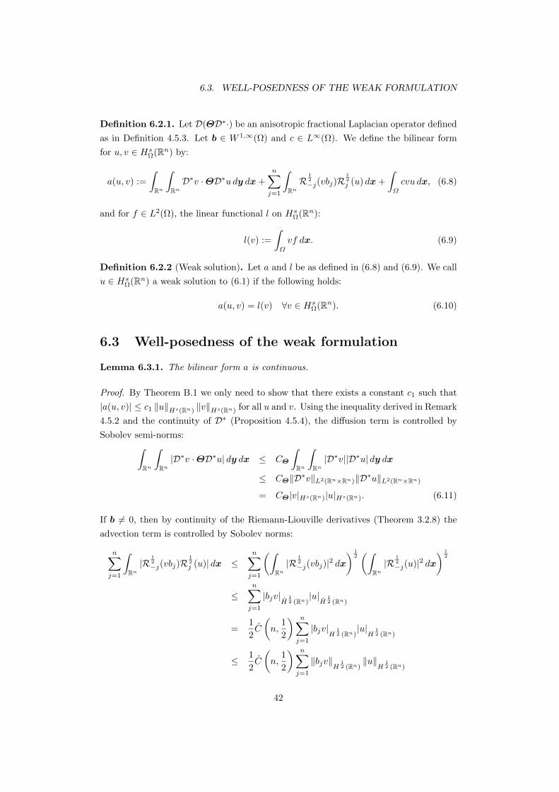
Definition 6.2.1. Let D(ΘD∗·) be an anisotropic fractional Laplacian operator defined
as in Definition 4.5.3. Let b ∈ W 1,∞(Ω) and c ∈ L∞(Ω). We define the bilinear form
for u, v ∈ HsΩ(Rn) by:
a(u, v) :=
∫Rn
∫RnD∗v ·ΘD∗u dy dx+
n∑j=1
∫RnR
12−j(vbj)R
12j (u) dx+
∫Ω
cvu dx, (6.8)
and for f ∈ L2(Ω), the linear functional l on HsΩ(Rn):
l(v) :=
∫Ω
vf dx. (6.9)
Definition 6.2.2 (Weak solution). Let a and l be as defined in (6.8) and (6.9). We call
u ∈ HsΩ(Rn) a weak solution to (6.1) if the following holds:
a(u, v) = l(v) ∀v ∈ HsΩ(Rn). (6.10)
6.3 Well-posedness of the weak formulation
Lemma 6.3.1. The bilinear form a is continuous.
Proof. By Theorem B.1 we only need to show that there exists a constant c1 such that
|a(u, v)| ≤ c1 ‖u‖Hs(Rn) ‖v‖Hs(Rn) for all u and v. Using the inequality derived in Remark
4.5.2 and the continuity of D∗ (Proposition 4.5.4), the diffusion term is controlled by
Sobolev semi-norms:∫Rn
∫Rn|D∗v ·ΘD∗u| dy dx ≤ CΘ
∫Rn
∫Rn|D∗v||D∗u| dy dx
≤ CΘ‖D∗v‖L2(Rn×Rn)‖D∗u‖L2(Rn×Rn)
= CΘ|v|Hs(Rn)|u|Hs(Rn). (6.11)
If b 6= 0, then by continuity of the Riemann-Liouville derivatives (Theorem 3.2.8) the
advection term is controlled by Sobolev norms:
n∑j=1
∫Rn|R
12−j(vbj)R
12j (u)| dx ≤
n∑j=1
(∫Rn|R
12−j(vbj)|
2 dx
) 12(∫
Rn|R
12−j(u)|2 dx
) 12
≤n∑j=1
|bjv|H
12 (Rn)
|u|H
12 (Rn)
=1
2C
(n,
1
2
) n∑j=1
|bjv|H
12 (Rn)
|u|H
12 (Rn)
≤ 1
2C
(n,
1
2
) n∑j=1
‖bjv‖H
12 (Rn)
‖u‖H
12 (Rn)
42
CHAPTER 6. WELL-POSEDNESS OF ELLIPTIC PROBLEMS
≤ 1
2C
(n,
1
2
) n∑j=1
Cbj , 12 ‖v‖H 12 (Rn)
‖u‖H
12 (Rn)
≤ C(b, n, s) ‖v‖Hs(Rn) ‖u‖Hs(Rn) , (6.12)
where
C(b, n, s) = Cemb
(s,
1
2
)C
(n,
1
2
) n∑j=1
Cbj , 12 . (6.13)
The constants and inequalities here come from Theorem 2.3.6, Theorem 2.4.3 and the
embedding Corollary 2.3.9. Finally, the reaction term is controlled by L2 norms:∫Ω
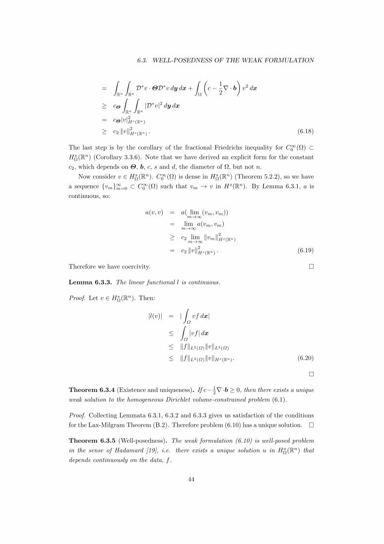
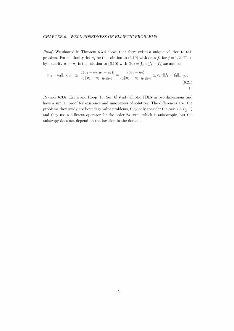
Remark 6.3.6. Ervin and Roop [16, Sec. 6] study elliptic FDEs in two dimensions and
have a similar proof for existence and uniqueness of solution. The differences are: the
problems they study are boundary value problems, they only consider the case s ∈ ( 12 , 1)
and they use a different operator for the order 2s term, which is anisotropic, but the
anistropy does not depend on the location in the domain.
45
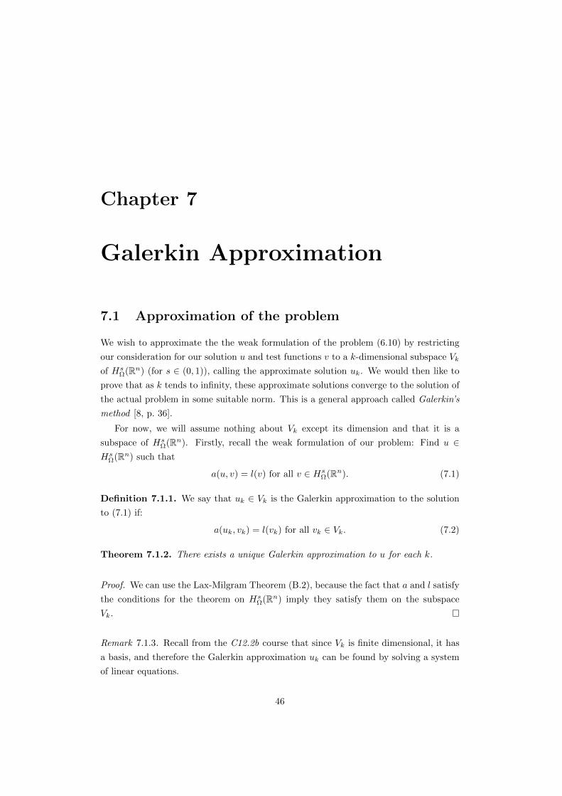
Chapter 7
Galerkin Approximation
7.1 Approximation of the problem
We wish to approximate the the weak formulation of the problem (6.10) by restricting
our consideration for our solution u and test functions v to a k-dimensional subspace Vk
of HsΩ(Rn) (for s ∈ (0, 1)), calling the approximate solution uk. We would then like to
prove that as k tends to infinity, these approximate solutions converge to the solution of
the actual problem in some suitable norm. This is a general approach called Galerkin’s
method [8, p. 36].
For now, we will assume nothing about Vk except its dimension and that it is a
subspace of HsΩ(Rn). Firstly, recall the weak formulation of our problem: Find u ∈
HsΩ(Rn) such that
a(u, v) = l(v) for all v ∈ HsΩ(Rn). (7.1)
Definition 7.1.1. We say that uk ∈ Vk is the Galerkin approximation to the solution
to (7.1) if:
a(uk, vk) = l(vk) for all vk ∈ Vk. (7.2)
Theorem 7.1.2. There exists a unique Galerkin approximation to u for each k.
Proof. We can use the Lax-Milgram Theorem (B.2), because the fact that a and l satisfy
the conditions for the theorem on HsΩ(Rn) imply they satisfy them on the subspace
Vk.
Remark 7.1.3. Recall from the C12.2b course that since Vk is finite dimensional, it has
a basis, and therefore the Galerkin approximation uk can be found by solving a system
of linear equations.
46
CHAPTER 7. GALERKIN APPROXIMATION
Definition 7.1.4. We say that the Galerkin approximation uk converges to the solution
u of (7.1) in the norm ‖ · ‖ on HsΩ(Rn) if:
‖u− uk‖HsΩ(Rn) → 0 as k →∞. (7.3)
7.2 Convergence in the Hs norm
The following lemma will give us a sufficient condition for convergence of the finite
element approximation in the Hs(Rn) norm.
Lemma 7.2.1 (Cea’s lemma). Let uk be the finite element approximation of (7.1),
and let c1 and c2 be the constants found in Lemmas 6.3.1 and 6.3.2 respectively for the
bilinear form a. Then:
‖u− uk‖Hs(Rn) ≤c1c2
infvk∈Vk
‖u− vk‖Hs(Rn) . (7.4)
Suppose futher that a is symmetric (i.e. b = 0). Then:
‖u− uk‖Hs(Rn) ≤√c1c2
infvk∈Vk
‖u− vk‖Hs(Rn) . (7.5)
Proof. See Finite Element Methods for Elliptic Problems, by Ciarley [8, Thm. 2.4.1,
Rmk. 2.4.1].
Theorem 7.2.2. A sufficient condition for convergence of the finite element approxi-
mation uk to the solution of (7.1) in the Hs(Rn) norm is that there exists a sequence of
operators Pk : HsΩ(Rn)→ Vk such that:
‖v − Pk(v)‖Hs(Rn) → 0 as k →∞, for all v ∈ HsΩ(Rn). (7.6)
Now we discuss examples of subspaces Vk and operators Pk such that this sufficient
condition holds.
7.3 Finite elements
As seen in the C12.2b course, we can consider the finite element spaces. We assume that
Ω is a polygonal domain, and triangulate it as usual with h > 0 being the length of the
longest side of any triangle in the mesh. The finite element space Vh ⊂ HsΩ(Rn) is the
space of all continuous, piecewise polynomials of degree m on the triangulation, where
m is a positive integer.
Theorem 7.3.1. Let s ∈ (0, 1), u ∈ HsΩ(Rn)). Then for real σ such that 0 ≤ s ≤ σ ≤ m
there exists a constant CI depending only on Ω such that:
‖u− Ihu‖Hs(Rn) ≤ CIhρ−s‖u‖Hσ(Ω) (7.7)
47
7.4. LEGENDRE POLYNOMIALS
Proof. See [4, Sec. 14.3] for a proof of:
‖u− Ihu‖Hs(Ω) ≤ Chρ−s‖u‖Hσ(Ω), (7.8)
for some constant C > 0. Then consider the theorem in [24, Thm. 11.4]. This theorem
implies that there exists a constant CΩ such that for any u ∈ HsΩ(Rn)
‖u‖Hs(Rn) ≤ CΩ‖u‖Hs(Ω). (7.9)
This gives the desired result with CI = C · CΩ.
The authors of [16] seem to have overlooked this issue. They quote the result (7.8),
but then use it as if the Hs(Ω) norm is equivalent to their Hs0(Ω) norm without justifi-
cation, which they define with the Fourier transform on R2.
7.4 Legendre polynomials
Let us consider the special case where Ω = [−1, 1], b = 0 and s ∈ (0, 12 ). The case s < 1
2
is interesting because the galerkin approximation need not be zero on the boundary (see
Section 2.6). It also simplifies matters because we don’t have to force our approximations
to have roots at −1 and 1. We can define the space Pk of polynomials of degree at most
k ∈ N and the operator Pk is the polynomial interpolant in k+ 1 Legendre points in Ω.
Theorem 7.4.1. Let s ∈ (0, 1), u ∈ HsΩ(Rn). Then for any real σ such that 0 ≤ s ≤ σ,
there exists a constant CP such that
‖u− Pku‖Hs(R) ≤ CPk3s/2−σ‖u‖Hσ(Ω). (7.10)
Proof. See [7, Thm. 2.4] for the bound:
‖u− Pku‖Hs(Ω) ≤ Ck3s/2−σ‖u‖Hσ(Ω), (7.11)
for some C > 0. Then note, as in Theorem 7.3.1, the continuous embedding of Hs(Ω)
into HsΩ(Rn) from [24, Thm. 11.4]. This gives the required inequality.
Corollary 7.4.2. Suppose that u is the solution to (7.1) for Ω = [−1, 1], b = 0 and
s ∈ (0, 12 ). Suppose further that u ∈ Hσ(Ω) where σ > 3s/2. Then the Galerkin
approximation uk to the problem (7.1) in the space Pk converges, and satisfies:
‖u− uk‖Hs(Rn) ≤√c1c2CPk
3s/2−σ‖u‖Hσ(Ω) (7.12)
Proof. Combine Cea’s Lemma 7.2.1 with the interpolation error estimate in Theorem
7.4.1.
48
Chapter 8
Conclusion
8.1 Aims of the project
When we proposed this project, we had an aim to develop a-posteriori error estimates
for a finite element method for an anomalous diffusion-type equation using the nonlocal
calculus. With these computable error estimates we wanted to implement an efficient
adaptive mesh algorithm.
However, the analysis of FDEs turned out to be much tougher than expected, pri-
marily because of the nonlocality of the fractional-order norms and operators, but it
certainly is interesting and it gave us a lot to study and write about. As a result, the
majority of this dissertation is devoted to the analytical side of FDEs, with just one
chapter devoted to approximation considerations.
8.2 Further work
We present ideas for further work in the form of a list:
• The issue with the nonlocal calculus for expressing the fractional Laplacian for
s ∈ [ 12 , 1) needs to be resolved. It is very frustrating that the authors have not
clarified this issue in their paper.
• The extension of the theoretical work to the time dependent case.
• Consider nonlocal Neumann-type volume constraints, as in [11].
• Practical implementation issues for Galerkin approximation of FDEs.
• Elliptic regularity estimates for fractional-order elliptic problems.
• Aubin-Nietsche argument for error bounds in the L2 norm.
49
Appendix A
The Fourier Transform
In this appendix we make clear which definition of the Fourier transform we use and
state some useful properties. We follow Partal Differential Equations, by Evans [17, p.
187-190]. We consider all functions to be complex-valued.
Definition A.1. For u ∈ L1(Rn) we define its Fourier transform F [u] = u and its
inverse Fourier transform F−1[u] = u by:
u(ξ) :=1
(2π)n/2
∫Rne−ix·ξu(x) dx, (A.1)
u(x) :=1
(2π)n/2
∫Rneiξ·xu(ξ) dξ, (A.2)
For u ∈ L2(Rn), the Fourier transform and inverse Fourier transform is defined using
the density of L1(Rn) ∩ L2(Rn) in L2(Rn) (see [17, p. 189]).
Theorem A.2 (Plancherel). Assume u ∈ L2(Rn). Then u, u ∈ L2(Rn) and
‖u‖L2(Rn) = ‖u‖L2(Rn) = ‖u‖L2(Rn) . (A.3)
Theorem A.3 (Parseval’s identity). Assume u, v ∈ L2(Rn). Then∫Rnuv dx =
∫Rnu¯v dξ. (A.4)
Proposition A.4 (Fourier transform of directional derivatives). Assume u ∈ Hk(Rn)
for some integer k ≥ 1 and m a unit vector in Rn. Let (m · ∇k) denote the kth-order
directional derivative in the direction m. Then
F[(m · ∇k)u
]= (m · iξ)ku (A.5)
50
Appendix B
Bilinear Forms on Hilbert
Spaces
Lemma B.1 (Criterion for continuity). Let H be a real Hilbert space and let a : H×H →R be a bilinear functional. Then a is continuous with respect to the product norms on
H ×H if and only if there exists a constant C > 0 such that:
a(u, v) ≤ C‖u‖H‖v‖H for all u, v ∈ H. (B.1)
Proof. Taught in the B4b Hilbert Spaces course, Hilary Term 2011.
Theorem B.2 (Lax-Milgram). Let H be a real Hilbert space, let l : H → R be a
continuous linear functional, and let a : H×H → R be a continuous bilinear functional,
that is also coercive i.e. there exists a constant c > 0 such that:
a(v, v) ≥ c‖v‖2H for all v ∈ H. (B.2)
Then there exists a unique solution to the problem of finding u ∈ H such that:
a(u, v) = l(v) for all v ∈ H. (B.3)
Proof. See Finite Element Methods for Elliptic Problems, by Ciarlet [8, p. 8] or Partial
Differential Equations, by Evans [17, p. 316].
51
Bibliography
[1] R. Adams, Sobolev Spaces, Academic Press, 1975.
[2] D. Benson, S. Wheatcraft, and M. Meerschaert, Application of a fractional
advection-dispersion equation, Water Resources Research, 36 (2000).
[3] , The fractional-order governing equation of levy motion, Water Resources
Research, 36 (2000), pp. 1413–1423.
[4] S. Brenner and L. Scott, The Mathematical Theory of Finite Element Methods,
Springer-Verlag, New York, 1994.
[5] H. Brezis, How to recognize constant functions. connections with sobolev spaces,
Russian Mathematical Surveys, 57 (2002), p. 693.
[6] K. Burrage, N. Hale, and D. Kay, An efficient implementation of an im-
plicit FEM scheme for fractional-in-space reaction-diffusion equations, Numerical
Analysis Technical Report, Oxford, (2011).
[7] C. Canuto and A. Quarteroni, Approximation results for orthogonal polyno-
mials in sobolev spaces., Math. Comput., 38 (1982), pp. 67–86.
[8] P. Ciarlet, The Finite Element Method for Elliptic Problems, North-Holland,
Amsterdam, 1978.
[9] E. Di Nezza, G. Palatucci, and E. Valdinoci, Hitchhiker’s guide to the frac-